Contents

I Introduction 1

1 Introduction To Advanced Algorithmic Trading . . . . . . . . . . . . . . . . . 31.1 Why Time Series Analysis, Bayesian Statistics and Machine Learning? . . . . . . 3

1.1.1 Bayesian Statistics . . . . . . . . . . . . . . . . . . . . . . . . . . . . . . . 41.1.2 Time Series Analysis . . . . . . . . . . . . . . . . . . . . . . . . . . . . . . 41.1.3 Machine Learning . . . . . . . . . . . . . . . . . . . . . . . . . . . . . . . 4

1.2 How Is The Book Laid Out? . . . . . . . . . . . . . . . . . . . . . . . . . . . . . . 51.3 Required Technical Background . . . . . . . . . . . . . . . . . . . . . . . . . . . . 5

1.3.1 Mathematics . . . . . . . . . . . . . . . . . . . . . . . . . . . . . . . . . . 51.3.2 Programming . . . . . . . . . . . . . . . . . . . . . . . . . . . . . . . . . . 6

1.4 How Does This Di�er From "Successful Algorithmic Trading"? . . . . . . . . . . 61.5 Software Installation . . . . . . . . . . . . . . . . . . . . . . . . . . . . . . . . . . 7

1.5.1 Installing Python . . . . . . . . . . . . . . . . . . . . . . . . . . . . . . . . 71.5.2 Installing R . . . . . . . . . . . . . . . . . . . . . . . . . . . . . . . . . . . 7

1.6 Backtesting Software Options . . . . . . . . . . . . . . . . . . . . . . . . . . . . . 71.6.1 Alternatives . . . . . . . . . . . . . . . . . . . . . . . . . . . . . . . . . . . 8

1.7 What Do You Get In The Rough Cut Version? . . . . . . . . . . . . . . . . . . . 8

II Bayesian Statistics 9

2 Introduction to Bayesian Statistics . . . . . . . . . . . . . . . . . . . . . . . . . 112.1 What is Bayesian Statistics? . . . . . . . . . . . . . . . . . . . . . . . . . . . . . . 11

2.1.1 Frequentist vs Bayesian Examples . . . . . . . . . . . . . . . . . . . . . . 122.2 Applying Bayes' Rule for Bayesian Inference . . . . . . . . . . . . . . . . . . . . . 142.3 Coin-Flipping Example . . . . . . . . . . . . . . . . . . . . . . . . . . . . . . . . . 15

3 Bayesian Inference of a Binomial Proportion . . . . . . . . . . . . . . . . . . . 193.1 The Bayesian Approach . . . . . . . . . . . . . . . . . . . . . . . . . . . . . . . . 193.2 Assumptions of the Approach . . . . . . . . . . . . . . . . . . . . . . . . . . . . . 203.3 Recalling Bayes' Rule . . . . . . . . . . . . . . . . . . . . . . . . . . . . . . . . . 203.4 The Likelihood Function . . . . . . . . . . . . . . . . . . . . . . . . . . . . . . . . 21

3.4.1 Bernoulli Distribution . . . . . . . . . . . . . . . . . . . . . . . . . . . . . 213.4.2 Bernoulli Likelihood Function . . . . . . . . . . . . . . . . . . . . . . . . . 223.4.3 Multiple Flips of the Coin . . . . . . . . . . . . . . . . . . . . . . . . . . . 22

3.5 Quantifying our Prior Beliefs . . . . . . . . . . . . . . . . . . . . . . . . . . . . . 223.5.1 Beta Distribution . . . . . . . . . . . . . . . . . . . . . . . . . . . . . . . . 233.5.2 Why Is A Beta Prior Conjugate to the Bernoulli Likelihood? . . . . . . . 253.5.3 Multiple Ways to Specify a Beta Prior . . . . . . . . . . . . . . . . . . . . 25

3.6 Using Bayes' Rule to Calculate a Posterior . . . . . . . . . . . . . . . . . . . . . . 26

4 Markov Chain Monte Carlo . . . . . . . . . . . . . . . . . . . . . . . . . . . . . . 294.1 Bayesian Inference Goals . . . . . . . . . . . . . . . . . . . . . . . . . . . . . . . . 294.2 Why Markov Chain Monte Carlo? . . . . . . . . . . . . . . . . . . . . . . . . . . 29

4.2.1 Markov Chain Monte Carlo Algorithms . . . . . . . . . . . . . . . . . . . 304.3 The Metropolis Algorithm . . . . . . . . . . . . . . . . . . . . . . . . . . . . . . . 30

1

2

4.4 Introducing PyMC3 . . . . . . . . . . . . . . . . . . . . . . . . . . . . . . . . . . 314.5 Inferring a Binomial Proportion with Markov Chain Monte Carlo . . . . . . . . . 32

4.5.1 Inferring a Binonial Proportion with Conjugate Priors Recap . . . . . . . 324.5.2 Inferring a Binonial Proportion with PyMC3 . . . . . . . . . . . . . . . . 32

4.6 Next Steps . . . . . . . . . . . . . . . . . . . . . . . . . . . . . . . . . . . . . . . 374.7 Bibliographic Note . . . . . . . . . . . . . . . . . . . . . . . . . . . . . . . . . . . 38

5 Bayesian Linear Regression . . . . . . . . . . . . . . . . . . . . . . . . . . . . . . 395.1 Frequentist Linear Regression . . . . . . . . . . . . . . . . . . . . . . . . . . . . . 395.2 Bayesian Linear Regression . . . . . . . . . . . . . . . . . . . . . . . . . . . . . . 405.3 Bayesian Linear Regression with PyMC3 . . . . . . . . . . . . . . . . . . . . . . . 41

5.3.1 What are Generalised Linear Models? . . . . . . . . . . . . . . . . . . . . 415.3.2 Simulating Data and Fitting the Model with PyMC3 . . . . . . . . . . . . 41

5.4 Next Steps . . . . . . . . . . . . . . . . . . . . . . . . . . . . . . . . . . . . . . . 455.5 Bibliographic Note . . . . . . . . . . . . . . . . . . . . . . . . . . . . . . . . . . . 465.6 Full Code . . . . . . . . . . . . . . . . . . . . . . . . . . . . . . . . . . . . . . . . 46

III Time Series Analysis 49

6 Introduction to Time Series Analysis . . . . . . . . . . . . . . . . . . . . . . . . 516.1 What is Time Series Analysis? . . . . . . . . . . . . . . . . . . . . . . . . . . . . 516.2 How Can We Apply Time Series Analysis in Quantitative Finance? . . . . . . . . 526.3 Time Series Analysis Software . . . . . . . . . . . . . . . . . . . . . . . . . . . . . 526.4 Time Series Analysis Roadmap . . . . . . . . . . . . . . . . . . . . . . . . . . . . 526.5 How Does This Relate to Other Statistical Tools? . . . . . . . . . . . . . . . . . . 53

7 Serial Correlation . . . . . . . . . . . . . . . . . . . . . . . . . . . . . . . . . . . . 557.1 Expectation, Variance and Covariance . . . . . . . . . . . . . . . . . . . . . . . . 55

7.1.1 Example: Sample Covariance in R . . . . . . . . . . . . . . . . . . . . . . 567.2 Correlation . . . . . . . . . . . . . . . . . . . . . . . . . . . . . . . . . . . . . . . 57

7.2.1 Example: Sample Correlation in R . . . . . . . . . . . . . . . . . . . . . . 587.3 Stationarity in Time Series . . . . . . . . . . . . . . . . . . . . . . . . . . . . . . 587.4 Serial Correlation . . . . . . . . . . . . . . . . . . . . . . . . . . . . . . . . . . . . 597.5 The Correlogram . . . . . . . . . . . . . . . . . . . . . . . . . . . . . . . . . . . . 60

7.5.1 Example 1 - Fixed Linear Trend . . . . . . . . . . . . . . . . . . . . . . . 617.5.2 Example 2 - Repeated Sequence . . . . . . . . . . . . . . . . . . . . . . . 61

7.6 Next Steps . . . . . . . . . . . . . . . . . . . . . . . . . . . . . . . . . . . . . . . 61

8 Random Walks and White Noise Models . . . . . . . . . . . . . . . . . . . . . . 658.1 Time Series Modelling Process . . . . . . . . . . . . . . . . . . . . . . . . . . . . 658.2 Backward Shift and Di�erence Operators . . . . . . . . . . . . . . . . . . . . . . 668.3 White Noise . . . . . . . . . . . . . . . . . . . . . . . . . . . . . . . . . . . . . . . 66

8.3.1 Second-Order Properties . . . . . . . . . . . . . . . . . . . . . . . . . . . . 678.3.2 Correlogram . . . . . . . . . . . . . . . . . . . . . . . . . . . . . . . . . . 67

8.4 Random Walk. . . . . . . . . . . . . . . . . . . . . . . . . . . . . . . . . . . . . . 688.4.1 Second-Order Properties . . . . . . . . . . . . . . . . . . . . . . . . . . . . 688.4.2 Correlogram . . . . . . . . . . . . . . . . . . . . . . . . . . . . . . . . . . 698.4.3 Fitting Random Walk Models to Financial Data . . . . . . . . . . . . . . 69

9 Autoregressive Moving Average Models . . . . . . . . . . . . . . . . . . . . . . 759.1 How Will We Proceed? . . . . . . . . . . . . . . . . . . . . . . . . . . . . . . . . . 759.2 Strictly Stationary . . . . . . . . . . . . . . . . . . . . . . . . . . . . . . . . . . . 769.3 Akaike Information Criterion . . . . . . . . . . . . . . . . . . . . . . . . . . . . . 769.4 Autoregressive (AR) Models of order p . . . . . . . . . . . . . . . . . . . . . . . . 77

9.4.1 Rationale . . . . . . . . . . . . . . . . . . . . . . . . . . . . . . . . . . . . 779.4.2 Stationarity for Autoregressive Processes . . . . . . . . . . . . . . . . . . 78

3

9.4.3 Second Order Properties . . . . . . . . . . . . . . . . . . . . . . . . . . . . 789.4.4 Simulations and Correlograms . . . . . . . . . . . . . . . . . . . . . . . . . 799.4.5 Financial Data . . . . . . . . . . . . . . . . . . . . . . . . . . . . . . . . . 82

9.5 Moving Average (MA) Models of order q . . . . . . . . . . . . . . . . . . . . . . . 879.5.1 Rationale . . . . . . . . . . . . . . . . . . . . . . . . . . . . . . . . . . . . 889.5.2 De�nition . . . . . . . . . . . . . . . . . . . . . . . . . . . . . . . . . . . . 889.5.3 Second Order Properties . . . . . . . . . . . . . . . . . . . . . . . . . . . . 889.5.4 Simulations and Correlograms . . . . . . . . . . . . . . . . . . . . . . . . . 899.5.5 Financial Data . . . . . . . . . . . . . . . . . . . . . . . . . . . . . . . . . 939.5.6 Next Steps . . . . . . . . . . . . . . . . . . . . . . . . . . . . . . . . . . . 98

9.6 Autogressive Moving Average (ARMA) Models of order p, q . . . . . . . . . . . . 999.6.1 Bayesian Information Criterion . . . . . . . . . . . . . . . . . . . . . . . . 999.6.2 Ljung-Box Test . . . . . . . . . . . . . . . . . . . . . . . . . . . . . . . . . 999.6.3 Rationale . . . . . . . . . . . . . . . . . . . . . . . . . . . . . . . . . . . . 1009.6.4 De�nition . . . . . . . . . . . . . . . . . . . . . . . . . . . . . . . . . . . . 1009.6.5 Simulations and Correlograms . . . . . . . . . . . . . . . . . . . . . . . . . 1009.6.6 Choosing the Best ARMA(p,q) Model . . . . . . . . . . . . . . . . . . . . 1049.6.7 Financial Data . . . . . . . . . . . . . . . . . . . . . . . . . . . . . . . . . 106

9.7 Next Steps . . . . . . . . . . . . . . . . . . . . . . . . . . . . . . . . . . . . . . . 107

10 Autoregressive Integrated Moving Average and Conditional HeteroskedasticModels . . . . . . . . . . . . . . . . . . . . . . . . . . . . . . . . . . . . . . . . . . 10910.1 Quick Recap . . . . . . . . . . . . . . . . . . . . . . . . . . . . . . . . . . . . . . 10910.2 Autoregressive Integrated Moving Average (ARIMA) Models of order p, d, q . . 110

10.2.1 Rationale . . . . . . . . . . . . . . . . . . . . . . . . . . . . . . . . . . . . 11010.2.2 De�nitions . . . . . . . . . . . . . . . . . . . . . . . . . . . . . . . . . . . 11010.2.3 Simulation, Correlogram and Model Fitting . . . . . . . . . . . . . . . . . 11110.2.4 Financial Data and Prediction . . . . . . . . . . . . . . . . . . . . . . . . 11310.2.5 Next Steps . . . . . . . . . . . . . . . . . . . . . . . . . . . . . . . . . . . 117

10.3 Volatility . . . . . . . . . . . . . . . . . . . . . . . . . . . . . . . . . . . . . . . . 11710.4 Conditional Heteroskedasticity . . . . . . . . . . . . . . . . . . . . . . . . . . . . 11710.5 Autoregressive Conditional Heteroskedastic Models . . . . . . . . . . . . . . . . . 118

10.5.1 ARCH De�nition . . . . . . . . . . . . . . . . . . . . . . . . . . . . . . . . 11810.5.2 Why Does This Model Volatility? . . . . . . . . . . . . . . . . . . . . . . . 11810.5.3 When Is It Appropriate To Apply ARCH(1)? . . . . . . . . . . . . . . . . 11910.5.4 ARCH(p) Models . . . . . . . . . . . . . . . . . . . . . . . . . . . . . . . . 119

10.6 Generalised Autoregressive Conditional Heteroskedastic Models . . . . . . . . . . 11910.6.1 GARCH De�nition . . . . . . . . . . . . . . . . . . . . . . . . . . . . . . . 11910.6.2 Simulations, Correlograms and Model Fittings . . . . . . . . . . . . . . . 12010.6.3 Financial Data . . . . . . . . . . . . . . . . . . . . . . . . . . . . . . . . . 122

10.7 Next Steps . . . . . . . . . . . . . . . . . . . . . . . . . . . . . . . . . . . . . . . 124

11 State Space Models and the Kalman Filter . . . . . . . . . . . . . . . . . . . . 12711.1 Linear State-Space Model . . . . . . . . . . . . . . . . . . . . . . . . . . . . . . . 12811.2 The Kalman Filter . . . . . . . . . . . . . . . . . . . . . . . . . . . . . . . . . . . 129

11.2.1 A Bayesian Approach . . . . . . . . . . . . . . . . . . . . . . . . . . . . . 12911.2.2 Prediction . . . . . . . . . . . . . . . . . . . . . . . . . . . . . . . . . . . . 130

IV Statistical Machine Learning 133

12 Model Selection and Cross-Validation . . . . . . . . . . . . . . . . . . . . . . . 13512.1 Bias-Variance Trade-O� . . . . . . . . . . . . . . . . . . . . . . . . . . . . . . . . 135

12.1.1 Machine Learning Models . . . . . . . . . . . . . . . . . . . . . . . . . . . 13512.1.2 Model Selection . . . . . . . . . . . . . . . . . . . . . . . . . . . . . . . . . 13612.1.3 The Bias-Variance Tradeo� . . . . . . . . . . . . . . . . . . . . . . . . . . 137

4

12.2 Cross-Validation . . . . . . . . . . . . . . . . . . . . . . . . . . . . . . . . . . . . 14012.2.1 Overview of Cross-Validation . . . . . . . . . . . . . . . . . . . . . . . . . 14012.2.2 Forecasting Example . . . . . . . . . . . . . . . . . . . . . . . . . . . . . . 14112.2.3 Validation Set Approach . . . . . . . . . . . . . . . . . . . . . . . . . . . . 14212.2.4 k-Fold Cross Validation . . . . . . . . . . . . . . . . . . . . . . . . . . . . 14212.2.5 Python Implementation . . . . . . . . . . . . . . . . . . . . . . . . . . . . 14312.2.6 k-Fold Cross Validation . . . . . . . . . . . . . . . . . . . . . . . . . . . . 14712.2.7 Full Python Code . . . . . . . . . . . . . . . . . . . . . . . . . . . . . . . 149

13 Kernel Methods and SVMs . . . . . . . . . . . . . . . . . . . . . . . . . . . . . . 15713.1 Support Vector Machines . . . . . . . . . . . . . . . . . . . . . . . . . . . . . . . 157

13.1.1 Motivation for Support Vector Machines . . . . . . . . . . . . . . . . . . . 15713.1.2 Advantages and Disadvantages of SVMs . . . . . . . . . . . . . . . . . . . 15813.1.3 Linear Separating Hyperplanes . . . . . . . . . . . . . . . . . . . . . . . . 15913.1.4 Classi�cation . . . . . . . . . . . . . . . . . . . . . . . . . . . . . . . . . . 16013.1.5 Deriving the Classi�er . . . . . . . . . . . . . . . . . . . . . . . . . . . . . 16113.1.6 Constructing the Maximal Margin Classi�er . . . . . . . . . . . . . . . . . 16213.1.7 Support Vector Classi�ers . . . . . . . . . . . . . . . . . . . . . . . . . . . 16313.1.8 Support Vector Machines . . . . . . . . . . . . . . . . . . . . . . . . . . . 165

13.2 Document Classi�cation using Support Vector Machines . . . . . . . . . . . . . . 16813.2.1 Overview . . . . . . . . . . . . . . . . . . . . . . . . . . . . . . . . . . . . 16813.2.2 Supervised Document Classi�cation . . . . . . . . . . . . . . . . . . . . . 169

13.3 Preparing a Dataset for Classi�cation . . . . . . . . . . . . . . . . . . . . . . . . 16913.3.1 Vectorisation . . . . . . . . . . . . . . . . . . . . . . . . . . . . . . . . . . 17813.3.2 Term-Frequency Inverse Document-Frequency . . . . . . . . . . . . . . . . 179

13.4 Training the Support Vector Machine . . . . . . . . . . . . . . . . . . . . . . . . 18013.4.1 Performance Metrics . . . . . . . . . . . . . . . . . . . . . . . . . . . . . . 181

13.5 Full Code Implementation in Python 3.4.x . . . . . . . . . . . . . . . . . . . . . . 18313.5.1 Biblographic Notes . . . . . . . . . . . . . . . . . . . . . . . . . . . . . . . 187

V Quantitative Trading Strategies 189

14 Introduction to QSTrader . . . . . . . . . . . . . . . . . . . . . . . . . . . . . . . 19114.1 Backtesting vs Live Trading . . . . . . . . . . . . . . . . . . . . . . . . . . . . . . 19114.2 Design Considerations . . . . . . . . . . . . . . . . . . . . . . . . . . . . . . . . . 192

14.2.1 Quantitative Trading Considerations . . . . . . . . . . . . . . . . . . . . . 19214.3 Installation . . . . . . . . . . . . . . . . . . . . . . . . . . . . . . . . . . . . . . . 193

15 ARIMA+GARCH Trading Strategy on Stock Market Indexes Using R . . . 19515.1 Strategy Overview . . . . . . . . . . . . . . . . . . . . . . . . . . . . . . . . . . . 19515.2 Strategy Implementation . . . . . . . . . . . . . . . . . . . . . . . . . . . . . . . . 19515.3 Strategy Results . . . . . . . . . . . . . . . . . . . . . . . . . . . . . . . . . . . . 19815.4 Full Code . . . . . . . . . . . . . . . . . . . . . . . . . . . . . . . . . . . . . . . . 201

Limit of Liability/Disclaimer ofWarranty

While the author has used their best e�orts in preparing this book, they make no representationsor warranties with the respect to the accuracy or completeness of the contents of this book andspeci�cally disclaim any implied warranties of merchantability or �tness for a particular purpose.It is sold on the understanding that the author is not engaged in rendering professional servicesand the author shall not be liable for damages arising herefrom. If professional advice or otherexpert assistance is required, the services of a competent professional should be sought.

i

ii

Part I

Introduction

1

Chapter 1

Introduction To AdvancedAlgorithmic Trading

In this introductory chapter we will consider why we want to adopt a fully statistical approach toquantitative trading and discuss Bayesian Statistics, Time Series Analysis and Machine Learning.

In addition we will look at what the book contains, the technical background you will needto get the most out of the book, why it di�ers from the previous book Successful AlgorithmicTrading and choices of backtesting software for the strategies we will discuss at the end of thebook.

1.1 Why Time Series Analysis, Bayesian Statistics and Ma-chine Learning?

In the last few years there has been a signi�cant increase in the availability of software forcarrying out statistical analysis at large scales, the so called "big data" era.

Much of this software is completely free, open source, extremely well tested and straightfor-ward to use. This coupled to the availability of �nancial data, as provided by services such asYahoo Finance, Google Finance, Quandl and IQ Feed, has lead to a sharp increase in individualslearning how to become a quantitative trader.

However, many of these individuals never get past learning basic "technical analysis" and soavoid important topics such as risk management, portfolio construction and algorithmic execu-tion. In addition they often neglect more e�ective means of generating alpha, such as can beprovided via detailed statistical analysis.

In this book I want to provide a "next step" for those who have already begun their algorithmictrading career, or are looking to try more advanced methods. In particular, we will be makinguse of techniques that are currently in deployment at some of the large quantitative hedge fundsand asset management �rms.

Our main area of study will be that of rigourous statistical analysis. This may sound likea dry topic, but I can assure you that not only is it extremely interesting when applied to realworld data, but it will provide you with a solid "mental framework" for how to think about allof your future trading methods and approaches.

Obviously, statistical analysis is a huge �eld of academic interest. Trying to distill the topicsimportant for quantitative trading is di�cult. However, there are three main areas that we willconcentrate on in this book:

� Bayesian Statistics

� Time Series Analysis

� Machine Learning

Each of these three areas has its place in quantitative �nance.

3

4

1.1.1 Bayesian Statistics

Bayesian Statistics is an alternative way of thinking about probability. The more traditional"frequentist" approach considers probabilities as the end result of many trials, for instance, thefairness of a coin being �ipped many times. Bayesian Statistics takes a di�erent approach andinstead considers probability as a measure of belief. That is, our own opinions are used to createprobability distributions from which the fairness of the coin might be based on.

While this may sound highly subjective, it is often an extremely e�ective method in practice.As new data arrives we can update our beliefs in a rational manner using the famous Bayes' Rule.Bayesian Statistics has found uses in many �elds, including engineering reliability, searching forlost nuclear submarines and controlling spacecraft orientation. However, it is also extremelyapplicable to quantitative trading problems.

Bayesian Inference is the application of Bayesian Statistics to making inference and predic-tions about data. In our case, we will be studying �nancial asset prices in order to predict futurevalues or understand why they change. The Bayesian framework provides us with a modern,sophisticated toolkit with which to carry this out.

Time Series Analysis and Machine Learning make heavy use of Bayesian Inference for thedesign of some of their algorithms. Hence it is essential that we understand the basics of howBayesian Statistics is carried out, particularly in relation to the Markov Chain Monte Carlomethod, which will we discuss at length in the book section on Bayesian Statistics.

To carry out Bayesian Inference in this book we will use a "probabilistic programming" tool,written in Python, called PyMC.

1.1.2 Time Series Analysis

Time Series Analysis provides a set of workhorse techniques for analysing �nancial time series.Most professional quants will begin their analysis of �nancial data using basic time series meth-ods. By studying the tools in time series analysis we can make elementary assessments of �nancialasset behaviour and use this to consider more advanced methods, in a structured way.

The main idea in Time Series Analysis is that of serial correlation. Brie�y, in terms ofdaily trading prices, serial correlation describes to us how much of today's asset prices arecorrelated to previous days' prices. Understanding the structure of this correlation helps us tobuild sophisticated models that can help us interpret the data and predict future values.

Time Series Analysis can be thought of as a much more rigourous approach to understand-ing the behaviour of �nancial asset prices than "technical analysis". While technical analysishas basic "indicators" for trends, mean reverting behaviour and volatility determination, timeseries analysis brings with it the full power of statistical inference, including hypothesis testing,goodness-of-�t tests and model selection, all of which serve to help us rigourously determine assetbehaviour and thus eventually increase our pro�tability of our strategies. We can understandtrends, seasonality, long-memory e�ects and volatility clustering in much more detail.

To carry out Time Series Analysis in this book we will use the R statistical programmingenvironment, along with its many external libraries.

1.1.3 Machine Learning

Machine Learning is another subset of statistical learning that applies modern statistical models,across huge data sets, whether they have a temporal component or not. Machine Learning ispart of the broader "data science" and quant ecosystem.

Machine Learning is generally subdivided into two separate categories, namely supervisedlearning and unsupervised learning. The former uses "training data" to train an algorithm todetect patterns in data. The latter has no concept of training (hence the "unsupervised") andalgorithms solely act on the data without being penalised or rewarded for correct answers.

We will be using machine learning techniques such as Support Vector Machines and RandomForests to �nd more complicated relationships between di�ering sets of �nancial data. If thesepatterns can be successfully validated then we can use them to infer structure in the data andmake predictions about future data points. Such tools are highly useful in alpha generation andrisk management.

5

To carry out Machine Learning in this book we will use the Python scikit-learn library, aswell as pandas, for data analysis.

1.2 How Is The Book Laid Out?

The book is broadly laid out in four sections. The �rst three are theoretical and teach you thebasics through to intermediate usage of Bayesian Statistics, Time Series Analysis and MachineLearning. The fourth section applies all of the previous theory to real trading strategies.

The book begins with a discussion on the Bayesian philosophy of statistics and uses thebinomial model as a simple example with which to apply Bayesian concepts such as conjugatepriors and posterior sampling via Markov Chain Monte Carlo.

It then explores Bayesian statistics as related to quantitative �nance, discussing key examplessuch as switch-point analysis (for regime detection) and stochastic volatility. Finally, we concludeby discussing the burgeoning area of Bayesian Econometrics.

In Time Series Analysis we begin by discussing the concept of Serial Correlation, beforeapplying it to simple models such as White Noise and the Random Walk. From these two modelswe can build up more sophisticated approaches to explaining Serial Correlation, culminating inthe Autoregressive Integrated Moving Average (ARIMA) family of models.

We then move on to consider volatility clustering, or conditional heteroskedasticity, and de-�ne and utilise the Generalised Autoregressive Conditional Heteroskedastic (GARCH) family ofmodels.

Subsequent to ARIMA and GARCH we will consider long-memory e�ects in �nancial timeseries, take a deeper look at cointegration (for statistical arbitrage) and consider approaches tostate space models including Hidden Markov Models and Kalman Filters.

All the while we will be applying these time series models to current �nancial data andassessing how they perform in terms of inference and prediction.

In the Machine Learning section we will begin with a more rigourous de�nition of supervisedand unsupervised learning, and then discuss the notation and methodology of statistical machinelearning. We will use the humble linear regression as our �rst model, swiftly moving on to linearclassi�cation with logistic regression, linear discriminant analysis and the Naive Bayes Classi�er.

We will then be ready to consider the more advanced non-linear methods such as Support Vec-tor Machines and Random Forests. We will consider unsupervised techniques such as PrincipalComponents Analysis, k-Means Clustering and Non-Negative Matrix Factorisation.

We will apply these techniques to asset price prediction, natural language processing andsubsequently sentiment analysis.

Finally we will discuss where to go from here. There are plenty of academic topics of interest toreview, including Non-Linear Time Series Methods, Bayesian Nonparametrics and Deep Learningusing Neural Networks. However, these topics will have to wait for later books!

1.3 Required Technical Background

Advanced Algorithmic Trading is a de�nite step up in complexity from Successful AlgorithmicTrading. Unfortunately it is di�cult to carry out any statistical inference without utilisingmathematics and programming.

1.3.1 Mathematics

To get the most out of this book it will be necessary to have taken introductory undergrad-uate classes in Mathematical Foundations, Calculus, Linear Algebra and Probability,which are often taught in university degrees of Mathematics, Physics, Engineering, Economics,Computer Science or similar.

Thankfully, you do not have to had a university education in order to use this book. Thereare plenty of fantastic resources for learning these topics on the internet. I prefer:

� Khan Academy - https://www.khanacademy.org

6

� MIT Open Courseware - http://ocw.mit.edu/index.htm

� Coursera - https://www.coursera.org

� Udemy - https://www.udemy.com

However, Bayesian Statistics, Time Series Analysis and Machine Learning are quantitativesubjects. There is no avoiding the fact that we will be using some intermediate mathematics toquantify our ideas.

I recommend the following courses for helping you get up to scratch with your mathematics:

� Linear Algebra by Gilbert Strang - http://ocw.mit.edu/courses/mathematics/18-06sc-linear-algebra-fall-2011/index.htm

� Single Variable Calculus by David Jerison - http://ocw.mit.edu/courses/mathematics/18-01-single-variable-calculus-fall-2006

� Multivariable Calculus by Denis Auroux - http://ocw.mit.edu/courses/mathematics/18-02-multivariable-calculus-fall-2007

� Probability by Santosh Venkatesh - https://www.coursera.org/course/probability

1.3.2 Programming

Since this book is fundamentally about programming quantitative trading strategies, it will benecessary to have some exposure to programming languages.

While it is not necessary to be an expert programmer or software developer, it is helpful tohave used a language similar to C++, C#, Java, Python, R or MatLab.

Many of you will likely have programmed in VB Script or VB.NET, through Excel. I wouldstrongly recommend taking some introductory Python and R programming courses if this is thecase as it will teach you about deeper programming topics that will be utilised in this book.

Here are some useful courses:

� Programming for Everybody - https://www.coursera.org/learn/python

� R Programming - https://www.coursera.org/course/rprog

1.4 How Does This Di�er From "Successful AlgorithmicTrading"?

Successful Algorithmic Trading was written primarily to help readers think in rigourous quantita-tive terms about their trading. In introduces the concepts of hypothesis testing and backtestingtrading strategies. It also outlined the available software that can be used to build backtestingsystems.

It discusses the means of storing �nancial data, measuring quantitative strategy performance,how to assess risk in quantitative strategies and how to optimise strategy performance. Finally, itprovides a template event-driven backtesting engine on which to base further, more sophisticated,trading systems.

It is not a book that provides many trading strategies. The emphasis is primarily on how tothink in a quantitative fashion and how to get started.

Advanced Algorithmic Trading has a di�erent focus. In this book the main topics are timeseries, machine learning and Bayesian stats, as applied to rigourous quantitative trading strategiesacross multiple asset classes.

Hence this book is largely theoretical for the �rst three sections and then highly practical forthe fourth, where we discuss the implementation of actual trading strategies.

I have added far more strategies to this book than in the previous version and this should giveyou a solid idea in how to continue researching and improving your own strategies and tradingideas.

7

This book is not a book that covers extensions of the event-driven backtester, nor does it dwellon software-speci�c testing methodology or how to build an institutional-grade infrastructuresystem. It is primarily about quantitative trading strategies and how to carry out research intotheir pro�tability.

1.5 Software Installation

Over the last few years it has become signi�cantly easier to get both Python and R environmentsinstalled on Windows, Mac OS X and Linux. In this section I'll describe how to easily installPython and R.

1.5.1 Installing Python

In order to follow the code for the Bayesian Statistics and Machine Learning chapters you willneed to install a Python environment.

Possibly the easiest way to achieve this is to download and install the free Anaconda distri-bution from Continuum Analytics at: https://www.continuum.io/downloads

The installation instructions are provided at the link above and come with all of the necessarylibraries you need to get going with the code in this book.

Once installed you will have access to the Spyder Integrated Development Environment (IDE),which provides a Python syntax-highlighting text editor, an IPython console for interactivework�ow and visualisation, and an object/variable explorer for helpful debugging.

All of the code in the Python sections of this book has been designed to be run using Ana-conda/Spyder for both Python 2.7.x and 3.4.x+, but will also happily work in "vanilla" Pythonvirtual environments, once the necessary libraries have been installed.

If you have any questions about Python installation, please email me at mike@quantstart.com.

1.5.2 Installing R

R is a little bit tricker to install than Anaconda, but not massively so. I make use of an IDEfor R, known as R Studio. This provides a similar interface to Anaconda, in that you get an Rsyntax-highlighting console and visualisation tools all in the same document interface.

R Studio requires R itself, so you must �rst download R before using R Studio. This can bedone for Windows, Mac OS X or Linux from the following link: https://cran.rstudio.com/

You'll want to select the pre-compiled binary from the top of the page that �ts your particularoperating system.

Once you have successfully installed R, the next step (if desired!) is to download R Studio:https://www.rstudio.com/products/rstudio/download/

Once again, you'll need to pick the version for your particular platform and operating systemtype (32/64-bit). You need to select one of the links under "Installers for Supported Platforms".

All of the code in the R sections of this book has been designed to be run using "vanilla" Rand/or R Studio.

If you have any questions about R installation, please email me at mike@quantstart.com.

1.6 Backtesting Software Options

These days, there are a myriad of options for carrying out backtests and new software (bothopen source and proprietary) appears every month.

I have decided to explain the strategies in simple terms and to concentrate predominantly onthe mathematical techniques. We will make use of vectorised (that is, non event-driven) systemspurely for reasons of speed and ease of implementation.

Python, via the pandas library, and R, both allow straightforward vectorised backtesting,which can give us a good �rst-order approximation to how well a strategy is likely to do inproduction.

8

Hence all performance �gures will be derived on the basis of these vectorised backtests andwe will discuss how much of an impact transaction costs are likely to have on performance.

1.6.1 Alternatives

There are many alternative backtesting environments available and I strongly encourage youto code up these strategies in more realistic environments if you wish to trade them in a liveenvironment. In particular, you could consider:

� QSForex - My own open-source high-frequency event-driven backtester for the Forex marketusing the OANDA brokerage: https://www.quantstart.com/qsforex

� Quantopian - A well-regarded web-based backtesting and trading engine for equities mar-kets: https://www.quantopian.com

� Zipline - An open source backtesting library that powers the Quantopian web-based back-tester: https://github.com/quantopian/zipline

1.7 What Do You Get In The Rough Cut Version?

Firstly, I'd like to thank you for pre-ordering the book in its 'rough cut' state. It is immenselyvaluable to me - and subsequently current and future readers - to have a continual process offeedback while the book is being �nished. For C++ For Quantitative Finance and SuccessfulAlgorithmic Trading I was able to incorporate many suggestions that came directly from readersof the site and the books.

Since this is a pre-order 'rough cut' release of Advanced Algorithmic Trading, not all of thetopics mentioned in the website ebook page will be available at this point in time. However,the book is continually being written and so as new content is produced it will be added to the'rough cut', prior to its full release early in 2016.

I have endeavoured to make sure that the Time Series Analysis section is nearly complete.It currently covers White Noise, Random Walks, ARMA, ARIMA, GARCH and State-SpaceModels. It is currently not covering Multivariate Models, Cointegration, Long-Memory E�ectsor Market Microstructure. However, the material covered up to the GARCH model alreadyprovides a very useful introduction to Time Series Analysis for those who have not considered itbefore. The remaining sections will be added in later releases.

The Bayesian Statistics section currently contains discussion on the basics of Bayesian Infer-ence and the analytical approach to inference on binomial proportions. This is su�cient materialnecessary to understand the later material on time series. It is currently not covering MarkovChain Monte Carlo techniques, Switch-Point Analysis, Stochastic Volatility or further BayesianEconometric tools. These will be added in later releases.

The Machine Learning section currently discusses two of the major issues in SupervisedLearning, namely the Bias-Variance Tradeo� and k-Fold Cross-Validation. It also discussesour �rst advanced machine learning technique, namely the Support Vector Machine. It currentlydoes not cover a broad introduction to Supervised and Unsupervised Learning, Linear Regression,Linear Classi�cation, Kernel Density Estimation, Tree-Based Methods, Unsupervised Learningand Natural Language Processing. These will be added in later releases.

The Quantitative Trading Strategies section currently only has a strategy based primarily onthe material from the Time Series section, namely the combined ARIMA+GARCH predictivemodel. It currently does not cover High Frequency Bid-Ask Spread Prediction, Asset ReturnsForecasting using Machine Learning techniques, Kalman Filters for Pairs Trading, VolatilityForecasting or Sentiment Analysis. These strategies, and more, will be added in later releases.

If there are any topics that you think would be particularly suitable for the book, then pleaseemail me at mike@quantstart.com and I'll do my best to try and incorporate them prior to the�nal release.

Part II

Bayesian Statistics

9

Chapter 2

Introduction to Bayesian Statistics

The �rst part of Advanced Algorithmic Trading is concerned with a detailed look at BayesianStatistics. As I mentioned in the introduction, Bayesian methods underpin many of the tech-niques in Time Series Analysis and Machine Learning, so it is essential that we gain an un-derstanding of the "philosophy" of the Bayesian approach and how to apply it to real worldquantitative �nance problems.

This chapter has been written to help you understand the basic ideas of Bayesian Statistics,and in particular, Bayes' Theorem (also known asBayes' Rule). We will see how the Bayesianapproach compares to the more traditional Classical, or Frequentist, approach to statisticsand the potential applications in both quantitative trading and risk management.

In the chapter we will:

� De�ne Bayesian statistics and Bayesian inference

� Compare Classical/Frequentist statistics and Bayesian statistics

� Derive the famous Bayes' Rule, an essential tool for Bayesian inference

� Interpret and apply Bayes' Rule for carrying out Bayesian inference

� Carry out a concrete probability coin-�ip example of Bayesian inference

2.1 What is Bayesian Statistics?

Bayesian statistics is a particular approach to applying probability to statistical prob-lems. It provides us with mathematical tools to update our beliefs about random events in lightof seeing new data or evidence about those events.

In particular Bayesian inference interprets probability as a measure of believability or con�-dence that an individual may possess about the occurance of a particular event.

We may have a prior belief about an event, but our beliefs are likely to change when new evi-dence is brought to light. Bayesian statistics gives us a solid mathematical means of incorporatingour prior beliefs, and evidence, to produce new posterior beliefs.

Bayesian statistics provides us with mathematical tools to rationally update our sub-jective beliefs in light of new data or evidence.

This is in contrast to another form of statistical inference, known as Classical or Frequentist,statistics, which assumes that probabilities are the frequency of particular random events occuringin a long run of repeated trials.

For example, as we roll a fair unweighted six-sided die repeatedly, we would see that eachnumber on the die tends to come up 1/6th of the time.

Frequentist statistics assumes that probabilities are the long-run frequency of randomevents in repeated trials.

11

12

When carrying out statistical inference, that is, inferring statistical information from proba-bilistic systems, the two approaches - Frequentist and Bayesian - have very di�erent philosophies.

Frequentist statistics tries to eliminate uncertainty by providing estimates. Bayesian statisticstries to preserve and re�ne uncertainty by adjusting individual beliefs in light of new evidence.

2.1.1 Frequentist vs Bayesian Examples

In order to make clear the distinction between the two di�ering statistical philosophies, we willconsider two examples of probabilistic systems:

� Coin �ips - What is the probability of an unfair coin coming up heads?

� Election of a particular candidate for UK Prime Minister - What is the probabilityof seeing an individual candidate winning, who has not stood before?

The following table describes the alternative philosophies of the frequentist and Bayesianapproaches:

Table 2.1: Comparison of Frequentist and Bayesian probability

Example Frequentist Interpretation Bayesian Interpretation

Unfair Coin Flip The probability of seeing a headwhen the unfair coin is �ippedis the long-run relative frequencyof seeing a head when repeated�ips of the coin are carried out.That is, as we carry out morecoin �ips the number of headsobtained as a proportion of thetotal �ips tends to the "true" or"physical" probability of the coincoming up as heads. In partic-ular the individual running theexperiment does not incorporatetheir own beliefs about the fair-ness of other coins.

Prior to any �ips of the coin anindividual may believe that thecoin is fair. After a few �ips thecoin continually comes up heads.Thus the prior belief about fair-ness of the coin is modi�ed toaccount for the fact that threeheads have come up in a row andthus the coin might not be fair.After 500 �ips, with 400 heads,the individual believes that thecoin is very unlikely to be fair.The posterior belief is heavilymodi�ed from the prior belief ofa fair coin.

Election of Candidate The candidate only ever standsonce for this particular electionand so we cannot perform "re-peated trials". In a frequen-tist setting we construct "vir-tual" trials of the election pro-cess. The probability of the can-didate winning is de�ned as therelative frequency of the candi-date winning in the "virtual" tri-als as a fraction of all trials.

An individual has a prior beliefof a candidate's chances of win-ning an election and their con-�dence can be quanti�ed as aprobability. However another in-dividual could also have a sepa-rate di�ering prior belief aboutthe same candidate's chances.As new data arrives, both beliefsare (rationally) updated by theBayesian procedure.

Thus in the Bayesian interpretation probability is a summary of an individual's opinion.A key point is that di�erent (rational, intelligent) individuals can have di�erent opinions (andthus di�erent prior beliefs), since they have di�ering access to data and ways of interpretingit. However, as both of these individuals come across new data that they both have access to,their (potentially di�ering) prior beliefs will lead to posterior beliefs that will begin convergingtowards each other, under the rational updating procedure of Bayesian inference.

13

In the Bayesian framework an individual would apply a probability of 0 when they haveno con�dence in an event occuring, while they would apply a probability of 1 when they areabsolutely certain of an event occuring. Assigning a probability between 0 and 1 allows weightedcon�dence in other potential outcomes.

In order to carry out Bayesian inference, we need to utilise a famous theorem in probabilityknown as Bayes' rule and interpret it in the correct fashion. In the following box, we deriveBayes' rule using the de�nition of conditional probability. However, it isn't essential to follow thederivation in order to use Bayesian methods, so feel free to skip the following section if youwish to jump straight into learning how to use Bayes' rule.

Deriving Bayes' Rule

We begin by considering the de�nition of conditional probability, which gives us a rule fordetermining the probability of an event A, given the occurance of another event B. An examplequestion in this vein might be "What is the probability of rain occuring given that there are cloudsin the sky?"

The mathematical de�nition of conditional probability is as follows:

P (A|B) =P (A ∩B)

P (B)(2.1)

This simply states that the probability of A occuring given that B has occured is equal tothe probability that they have both occured, relative to the probability that B has occured.

Or in the language of the example above: The probability of rain given that we have seenclouds is equal to the probability of rain and clouds occuring together, relative to the probabilityof seeing clouds at all.

If we multiply both sides of this equation by P (B) we get:

P (B)P (A|B) = P (A ∩B) (2.2)

But, we can simply make the same statement about P (B|A), which is akin to asking "Whatis the probability of seeing clouds, given that it is raining?" :

P (B|A) =P (B ∩A)

P (A)(2.3)

Note that P (A∩B) = P (B ∩A) and so by substituting the above and multiplying by P (A),we get:

P (A)P (B|A) = P (A ∩B) (2.4)

We are now able to set the two expressions for P (A ∩B) equal to each other:

P (B)P (A|B) = P (A)P (B|A) (2.5)

If we now divide both sides by P (B) we arrive at the celebrated Bayes' rule:

P (A|B) =P (B|A)P (A)

P (B)(2.6)

However, it will be helpful for later usage of Bayes' rule to modify the denominator, P (B)on the right hand side of the above relation to be written in terms of P (B|A). We can actuallywrite:

14

P (B) =∑a∈A

P (B ∩A) (2.7)

This is possible because the events A are an exhaustive partition of the sample space.So that by substituting the de�ntion of conditional probability we get:

P (B) =∑a∈A

P (B ∩A) =∑a∈A

P (B|A)P (A) (2.8)

Finally, we can substitute this into Bayes' rule from above to obtain an alternative version ofBayes' rule, which is used heavily in Bayesian inference:

P (A|B) =P (B|A)P (A)∑a∈A P (B|A)P (A)

(2.9)

Now that we have derived Bayes' rule we are able to apply it to statistical inference.

2.2 Applying Bayes' Rule for Bayesian Inference

As we stated at the start of this chapter the basic idea of Bayesian inference is to continuallyupdate our prior beliefs about events as new evidence is presented. This is a very natural wayto think about probabilistic events. As more and more evidence is accumulated our prior beliefsare steadily "washed out" by any new data.

Consider a (rather nonsensical) prior belief that the Moon is going to collide with the Earth.For every night that passes, the application of Bayesian inference will tend to correct our priorbelief to a posterior belief that the Moon is less and less likely to collide with the Earth, since itremains in orbit.

In order to demonstrate a concrete numerical example of Bayesian inference it is necessaryto introduce some new notation.

Firstly, we need to consider the concept of parameters and models. A parameter could bethe weighting of an unfair coin, which we could label as θ. Thus θ = P (H) would describe theprobability distribution of our beliefs that the coin will come up as heads when �ipped. Themodel is the actual means of encoding this �ip mathematically. In this instance, the coin �ipcan be modelled as a Bernoulli trial.

Bernoulli Trial

A Bernoulli trial is a random experiment with only two outcomes, usually labelled as "success"or "failure", in which the probability of the success is exactly the same every time the trial iscarried out. The probability of the success is given by θ, which is a number between 0 and 1.Thus θ ∈ [0, 1].

Over the course of carrying out some coin �ip experiments (repeated Bernoulli trials) we willgenerate some data, D, about heads or tails.

A natural example question to ask is "What is the probability of seeing 3 heads in 8 �ips (8Bernoulli trials), given a fair coin (θ = 0.5)?".

A model helps us to ascertain the probability of seeing this data, D, given a value of theparameter θ. The probability of seeing data D under a particular value of θ is given by thefollowing notation: P (D|θ).

However, if you consider it for a moment, we are actually interested in the alternative question- "What is the probability that the coin is fair (or unfair), given that I have seen a particularsequence of heads and tails?".

Thus we are interested in the probability distribution which re�ects our belief about di�erentpossible values of θ, given that we have observed some data D. This is denoted by P (θ|D).Notice that this is the converse of P (D|θ). So how do we get between these two probabilities?It turns out that Bayes' rule is the link that allows us to go between the two situations.

15

Bayes' Rule for Bayesian Inference

P (θ|D) = P (D|θ) P (θ) / P (D) (2.10)

Where:

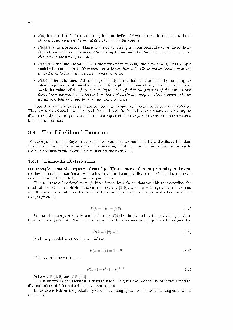
� P (θ) is the prior. This is the strength in our belief of θ without considering the evidenceD. Our prior view on the probability of how fair the coin is.

� P (θ|D) is the posterior. This is the (re�ned) strength of our belief of θ once the evidenceD has been taken into account. After seeing 4 heads out of 8 �ips, say, this is our updatedview on the fairness of the coin.

� P (D|θ) is the likelihood. This is the probability of seeing the data D as generated by amodel with parameter θ. If we knew the coin was fair, this tells us the probability of seeinga number of heads in a particular number of �ips.

� P (D) is the evidence. This is the probability of the data as determined by summing (orintegrating) across all possible values of θ, weighted by how strongly we believe in thoseparticular values of θ. If we had multiple views of what the fairness of the coin is (butdidn't know for sure), then this tells us the probability of seeing a certain sequence of �ipsfor all possibilities of our belief in the coin's fairness.

The entire goal of Bayesian inference is to provide us with a rational and mathematicallysound procedure for incorporating our prior beliefs, with any evidence at hand, in order toproduce an updated posterior belief. What makes it such a valuable technique is that posteriorbeliefs can themselves be used as prior beliefs under the generation of new data. Hence Bayesianinference allows us to continually adjust our beliefs under new data by repeatedly applying Bayes'rule.

There was a lot of theory to take in within the previous two sections, so I'm now going toprovide a concrete example using the age-old tool of statisticians: the coin-�ip.

2.3 Coin-Flipping Example

In this example we are going to consider multiple coin-�ips of a coin with unknown fairness. Wewill use Bayesian inference to update our beliefs on the fairness of the coin as more data (i.e.more coin �ips) becomes available. The coin will actually be fair, but we won't learn this untilthe trials are carried out. At the start we have no prior belief on the fairness of the coin, thatis, we can say that any level of fairness is equally likely.

In statistical language we are going to perform N repeated Bernoulli trials with θ = 0.5. Wewill use a uniform distribution as a means of characterising our prior belief that we are unsureabout the fairness. This states that we consider each level of fairness (or each value of θ) to beequally likely.

We are going to use a Bayesian updating procedure to go from our prior beliefs to posteriorbeliefs as we observe new coin �ips. This is carried out using a particularly mathematicallysuccinct procedure via the concept of conjugate priors. We won't go into any detail on conjugatepriors within this chapter, as it will form the basis of the next chapter on Bayesian inference. Itwill however provide us with the means of explaining how the coin �ip example is carried out inpractice.

The uniform distribution is actually a more speci�c case of another probability distribution,known as a Beta distribution. Conveniently, under the binomial model, if we use a Beta distri-bution for our prior beliefs it leads to a Beta distribution for our posterior beliefs. This is anextremely useful mathematical result, as Beta distributions are quite �exible in modelling beliefs.However, I don't want to dwell on the details of this too much here, since we will discuss it inthe next chapter. At this stage, it just allows us to easily create some visualisations below thatemphasises the Bayesian procedure!

16

In the following �gure we can see 6 particular points at which we have carried out a numberof Bernoulli trials (coin �ips). In the �rst sub-plot we have carried out no trials and hence ourprobability density function (in this case our prior density) is the uniform distribution. It statesthat we have equal belief in all values of θ representing the fairness of the coin.

The next panel shows 2 trials carried out and they both come up heads. Our Bayesianprocedure using the conjugate Beta distributions now allows us to update to a posterior density.Notice how the weight of the density is now shifted to the right hand side of the chart. Thisindicates that our prior belief of equal likelihood of fairness of the coin, coupled with 2 new datapoints, leads us to believe that the coin is more likely to be unfair (biased towards heads) thanit is tails.

The following two panels show 10 and 20 trials respectively. Notice that even though wehave seen 2 tails in 10 trials we are still of the belief that the coin is likely to be unfair andbiased towards heads. After 20 trials, we have seen a few more tails appear. The density of theprobability has now shifted closer to θ = P (H) = 0.5. Hence we are now starting to believe thatthe coin is possibly fair.

After 50 and 500 trials respectively, we are now beginning to believe that the fairness ofthe coin is very likely to be around θ = 0.5. This is indicated by the shrinking width of theprobability density, which is now clustered tightly around θ = 0.46 in the �nal panel. Were we tocarry out another 500 trials (since the coin is actually fair) we would see this probability densitybecome even tighter and centred closer to θ = 0.5.

Figure 2.1: Bayesian update procedure using the Beta-Binomial Model

Thus it can be seen that Bayesian inference gives us a rational procedure to go from anuncertain situation with limited information to a more certain situation with signi�cant amountsof data. In the next chapter we will discuss the notion of conjugate priors in more depth, whichheavily simplify the mathematics of carrying out Bayesian inference in this example.

For completeness, I've provided the Python code (heavily commented) for producing thisplot. It makes use of SciPy's statistics model, in particular, the Beta distribution:

17

# beta_binomial.py

import numpy as npfrom scipy import statsfrom matplotlib import pyplot as plt

if __name__ == "__main__":# Create a list of the number of coin tosses ("Bernoulli trials")number_of_trials = [0, 2, 10, 20, 50, 500]

# Conduct 500 coin tosses and output into a list of 0s and 1s# where 0 represents a tail and 1 represents a headdata = stats.bernoulli.rvs(0.5, size=number_of_trials[-1])

# Discretise the x-axis into 100 separate plotting pointsx = np.linspace(0, 1, 100)

# Loops over the number_of_trials list to continually add# more coin toss data. For each new set of data, we update# our (current) prior belief to be a new posterior. This is# carried out using what is known as the Beta-Binomial model.# For the time being, we won’t worry about this too much.for i, N in enumerate(number_of_trials):

# Accumulate the total number of heads for this# particular Bayesian updateheads = data[:N].sum()

# Create an axes subplot for each updateax = plt.subplot(len(number_of_trials) / 2, 2, i + 1)ax.set_title("%s trials, %s heads" % (N, heads))

# Add labels to both axes and hide labels on y-axisplt.xlabel("$P(H)$, Probability of Heads")plt.ylabel("Density")if i == 0:

plt.ylim([0.0, 2.0])plt.setp(ax.get_yticklabels(), visible=False)

# Create and plot a Beta distribution to represent the# posterior belief in fairness of the coin.y = stats.beta.pdf(x, 1 + heads, 1 + N - heads)plt.plot(x, y, label="observe %d tosses,\n %d heads" % (N, heads))plt.fill_between(x, 0, y, color="#aaaadd", alpha=0.5)

# Expand plot to cover full width/height and show itplt.tight_layout()plt.show()

18

Chapter 3

Bayesian Inference of a BinomialProportion

In the previous chapter we examined Bayes' rule and considered how it allowed us to rationallyupdate beliefs about uncertainty as new evidence came to light. We mentioned brie�y thatsuch techniques are becoming extremely important in the �elds of data science and quantitative�nance.

In this chapter we are going to expand on the coin-�ip example that we studied in the previouschapter by discussing the notion of Bernoulli trials, the beta distribution and conjugate priors.

Our goal in this chapter is to allow us to carry out what is known as "inference on a binomialproportion". That is, we will be studying probabilistic situations with two outcomes (e.g. acoin-�ip) and trying to estimate the proportion of a repeated set of events that come up headsor tails.

Our goal is to estimate how fair a coin is. We will use that estimate to makepredictions about how many times it will come up heads when we �ip it in the future.

While this may sound like a rather academic example, it is actually substantially more ap-plicable to real-world applications than may �rst appear. Consider the following scenarios:

� Engineering: Estimating the proportion of aircraft turbine blades that possess a struc-tural defect after fabrication

� Social Science: Estimating the proportion of individuals who would respond "yes" on acensus question

� Medical Science: Estimating the proportion of patients who make a full recovery aftertaking an experimental drug to cure a disease

� Corporate Finance: Estimating the proportion of transactions in error when carryingout �nancial audits

� Data Science: Estimating the proportion of individuals who click on an ad when visitinga website

As can be seen, inference on a binomial proportion is an extremely important statisticaltechnique and will form the basis of many of the chapters on Bayesian statistics that follow.

3.1 The Bayesian Approach

While we motivated the concept of Bayesian statistics in the previous chapter, I want to outline�rst how our analysis will proceed. This will motivate the following sections and give you a"bird's eye view" of what the Bayesian approach is all about.

19

20

As we stated above, our goal is estimate the fairness of a coin. Once we have an estimate forthe fairness, we can use this to predict the number of future coin �ips that will come up heads.

We will learn about the speci�c techniques as we go while we cover the following steps:

1. Assumptions - We will assume that the coin has two outcomes (i.e. it won't land on itsside), the �ips will appear randomly and will be completely independent of each other. Thefairness of the coin will also be stationary, that is it won't alter over time. We will denotethe fairness by the parameter θ. We will be considering stationary processes in depth inthe section on Time Series Analysis later in the book.

2. Prior Beliefs - To carry out a Bayesian analysis, we must quantify our prior beliefs aboutthe fairness of the coin. This comes down to specifying a probability distribution on ourbeliefs of this fairness. We will use a relatively �exible probability distribution called thebeta distribution to model our beliefs.

3. Experimental Data - We will carry out some (virtual) coin-�ips in order to give us somehard data. We will count the number of heads z that appear in N �ips of the coin. We willalso need a way of determining the probability of such results appearing, given a particularfairness, θ, of the coin. For this we will need to discuss likelihood functions, and inparticular the Bernoulli likelihood function.

4. Posterior Beliefs - Once we have a prior belief and a likelihood function, we can useBayes' rule in order to calculate a posterior belief about the fairness of the coin. We coupleour prior beliefs with the data we have observed and update our beliefs accordingly. Luckilyfor us, if we use a beta distribution as our prior and a Bernoulli likelihood we also get abeta distribution as a posterior. These are known as conjugate priors.

5. Inference - Once we have a posterior belief we can estimate the coin's fairness θ, predictthe probability of heads on the next �ip or even see how the results depend upon di�erentchoices of prior beliefs. The latter is known as model comparison.

At each step of the way we will be making visualisations of each of these functions anddistributions using the relatively recent Seaborn plotting package for Python. Seaborn sits "ontop" of Matplotlib, but has far better defaults for statistical plotting.

3.2 Assumptions of the Approach

As with all models we need to make some assumptions about our situation.

� We are going to assume that our coin can only have two outcomes, that is it can only landon its head or tail and never on its side

� Each �ip of the coin is completely independent of the others, i.e. we have independent andidentically distributed (i.i.d.) coin �ips

� The fairness of the coin does not change in time, that is it is stationary

With these assumptions in mind, we can now begin discussing the Bayesian procedure.

3.3 Recalling Bayes' Rule

In the the previous chapter we outlined Bayes' rule. I've repeated it here for completeness:

P (θ|D) = P (D|θ) P (θ) / P (D) (3.1)

Where:

21

� P (θ) is the prior. This is the strength in our belief of θ without considering the evidenceD. Our prior view on the probability of how fair the coin is.

� P (θ|D) is the posterior. This is the (re�ned) strength of our belief of θ once the evidenceD has been taken into account. After seeing 4 heads out of 8 �ips, say, this is our updatedview on the fairness of the coin.

� P (D|θ) is the likelihood. This is the probability of seeing the data D as generated by amodel with parameter θ. If we knew the coin was fair, this tells us the probability of seeinga number of heads in a particular number of �ips.

� P (D) is the evidence. This is the probability of the data as determined by summing (orintegrating) across all possible values of θ, weighted by how strongly we believe in thoseparticular values of θ. If we had multiple views of what the fairness of the coin is (butdidn't know for sure), then this tells us the probability of seeing a certain sequence of �ipsfor all possibilities of our belief in the coin's fairness.

Note that we have three separate components to specify, in order to calcute the posterior.They are the likelihood, the prior and the evidence. In the following sections we are going todiscuss exactly how to specify each of these components for our particular case of inference on abinomial proportion.

3.4 The Likelihood Function

We have just outlined Bayes' rule and have seen that we must specify a likelihood function,a prior belief and the evidence (i.e. a normalising constant). In this section we are going toconsider the �rst of these components, namely the likelihood.

3.4.1 Bernoulli Distribution

Our example is that of a sequence of coin �ips. We are interested in the probability of the coincoming up heads. In particular, we are interested in the probability of the coin coming up headsas a function of the underlying fairness parameter θ.

This will take a functional form, f . If we denote by k the random variable that describes theresult of the coin toss, which is drawn from the set {1, 0}, where k = 1 represents a head andk = 0 represents a tail, then the probability of seeing a head, with a particular fairness of thecoin, is given by:

P (k = 1|θ) = f(θ) (3.2)

We can choose a particularly succint form for f(θ) by simply stating the probability is givenby θ itself, i.e. f(θ) = θ. This leads to the probability of a coin coming up heads to be given by:

P (k = 1|θ) = θ (3.3)

And the probability of coming up tails as:

P (k = 0|θ) = 1− θ (3.4)

This can also be written as:

P (k|θ) = θk(1− θ)1−k (3.5)

Where k ∈ {1, 0} and θ ∈ [0, 1].This is known as the Bernoulli distribution. It gives the probability over two separate,

discrete values of k for a �xed fairness parameter θ.In essence it tells us the probability of a coin coming up heads or tails depending on how fair

the coin is.

22

3.4.2 Bernoulli Likelihood Function

We can also consider another way of looking at the above function. If we consider a �xedobservation, i.e. a known coin �ip outcome, k, and the fairness parameter θ as a continuousvariable then:

P (k|θ) = θk(1− θ)1−k (3.6)

tells us the probability of a �xed outcome k given some particular value of θ. As we adjust θ(e.g. change the fairness of the coin), we will start to see di�erent probabilities for k.

This is known as the likelihood function of θ. It is a function of a continuous θ and di�ersfrom the Bernoulli distribution because the latter is actually a discrete probability distributionover two potential outcomes of the coin-�ip k.

Note that the likelihood function is not actually a probability distribution in the true sensesince integrating it across all values of the fairness parameter θ does not actually equal 1, as isrequired for a probability distribution.

We say that P (k|θ) = θk(1− θ)1−k is the Bernoulli likelihood function for θ.

3.4.3 Multiple Flips of the Coin

Now that we have the Bernoulli likelihood function we can use it to determine the probability ofseeing a particular sequence of N �ips, given by the set {k1, ..., kN}.

Since each of these �ips is independent of any other, the probability of the sequence occuringis simply the product of the probability of each �ip occuring.

If we have a particular fairness parameter θ, then the probability of seeing this particularstream of �ips, given θ, is given by:

P ({k1, ..., kN}|θ) =∏i

P (ki|θ) (3.7)

=∏i

θki(1− θ)1−ki (3.8)

What if we are interested in the number of heads, say, in N �ips? If we denote by z thenumber of heads appearing, then the formula above becomes:

P (z,N |θ) = θz(1− θ)N−z (3.9)

That is, the probability of seeing z heads, in N �ips, assuming a fairness parameter θ. Wewill use this formula when we come to determine our posterior belief distribution later in thechapter.

3.5 Quantifying our Prior Beliefs

An extremely important step in the Bayesian approach is to determine our prior beliefs and then�nd a means of quantifying them.

In the Bayesian approach we need to determine our prior beliefs on parameters andthen �nd a probability distribution that quanti�es these beliefs.

In this instance we are interested in our prior beliefs on the fairness of the coin. That is, wewish to quantify our uncertainty in how biased the coin is.

To do this we need to understand the range of values that θ can take and how likely we thinkeach of those values are to occur.

θ = 0 indicates a coin that always comes up tails, while θ = 1 implies a coin that alwayscomes up heads. A fair coin is denoted by θ = 0.5. Hence θ ∈ [0, 1]. This implies that ourprobability distribution must also exist on the interval [0, 1].

The question then becomes - which probability distribution do we use to quantify our beliefsabout the coin?

23

3.5.1 Beta Distribution

In this instance we are going to choose the beta distribution. The probability density function(PDF) of the beta distribution is given by the following:

P (θ|α, β) = θα−1(1− θ)β−1/B(α, β) (3.10)

Where the term in the denominator, B(α, β) is present to act as a normalising constant sothat the area under the PDF actually sums to 1.

I've plotted a few separate realisations of the beta distribution for various parameters α andβ in Figure 3.1.

Figure 3.1: Di�erent realisations of the beta distribution for various parameters α and β.

To plot the image yourself, you will need to install seaborn:

pip install seaborn

The Python code to produce the plot is given below:

# beta_plot.py

import numpy as npfrom scipy.stats import betaimport matplotlib.pyplot as pltimport seaborn as sns

if __name__ == "__main__":sns.set_palette("deep", desat=.6)sns.set_context(rc={"figure.figsize": (8, 4)})x = np.linspace(0, 1, 100)params = [

24

(0.5, 0.5),(1, 1),(4, 3),(2, 5),(6, 6)

]for p in params:

y = beta.pdf(x, p[0], p[1])plt.plot(x, y, label="$\\alpha=%s$, $\\beta=%s$" % p)

plt.xlabel("$\\theta$, Fairness")plt.ylabel("Density")plt.legend(title="Parameters")plt.show()

Essentially, as α becomes larger the bulk of the probability distribution moves towards theright (a coin biased to come up heads more often), whereas an increase in β moves the distributiontowards the left (a coin biased to come up tails more often).

However, if both α and β increase then the distribution begins to narrow. If α and β increaseequally, then the distribution will peak over θ = 0.5, i.e. when the coin is far.

Why have we chosen the beta function as our prior? There are a couple of reasons:

� Support - It's de�ned on the interval [0, 1], which is the same interval that θ exists over.

� Flexibility - It possesses two shape parameters known as α and β, which give it signi�cant�exibility. This �exibility provides us with a lot of choice in how we model our beliefs.

However, perhaps the most important reason for choosing a beta distribution is because it isa conjugate prior for the Bernoulli distribution.

Conjugate Priors

In Bayes' rule above we can see that the posterior distribution is proportional to the product ofthe prior distribution and the likelihood function:

P (θ|D) ∝ P (D|θ)P (θ) (3.11)

A conjugate prior is a choice of prior distribution, that when coupled with a speci�c typeof likelihood function, provides a posterior distribution that is of the same family as the priordistribution.

The prior and posterior both have the same probability distribution family, but with di�eringparameters.

Conjugate priors are extremely convenient from a calculation point of view as they provideclosed-form expressions for the posterior, thus negating any complex numerical integration.

In our case, if we use a Bernoulli likelihood function AND a beta distribution as the choiceof our prior, we immediately know that the posterior will also be a beta distribution.

Using a beta distribution for the prior in this manner means that we can carry out moreexperimental coin �ips and straightforwardly re�ne our beliefs. The posterior will become thenew prior and we can use Bayes' rule successively as new coin �ips are generated.

If our prior belief is speci�ed by a beta distribution and we have a Bernoulli likelihoodfunction, then our posterior will also be a beta distribution.

Note however that a prior is only conjugate with respect to a particular likelihood function.

25

3.5.2 Why Is A Beta Prior Conjugate to the Bernoulli Likelihood?

We can actually use a simple calculation to prove why the choice of the beta distribution for theprior, with a Bernoulli likelihood, gives a beta distribution for the posterior.

As mentioned above, the probability density function of a beta distribution, for our particularparameter θ, is given by:

P (θ|α, β) = θα−1(1− θ)β−1/B(α, β) (3.12)

You can see that the form of the beta distribution is similar to the form of a Bernoullilikelihood. In fact, if you multiply the two together (as in Bayes' rule), you get:

θα−1(1− θ)β−1/B(α, β)× θk(1− θ)1−k ∝ θα+k−1(1− θ)β+k (3.13)

Notice that the term on the right hand side of the proportionality sign has the same form asour prior (up to a normalising constant).

3.5.3 Multiple Ways to Specify a Beta Prior

At this stage we've discussed the fact that we want to use a beta distribution in order to specifyour prior beliefs about the fairness of the coin. However, we only have two parameters to playwith, namely α and β.

How do these two parameters correspond to our more intuitive sense of "likely fairness" and"uncertainty in fairness"?

Well, these two concepts neatly correspond to the mean and the variance of the beta distribu-tion. Hence, if we can �nd a relationship between these two values and the α and β parameters,we can more easily specify our beliefs.

It turns out that the mean µ is given by:

µ =α

α+ β(3.14)

While the standard deviation σ is given by:

σ =

√αβ

(α+ β)2(α+ β + 1)(3.15)

Hence, all we need to do is re-arrange these formulae to provide α and β in terms of µ andσ. α is given by:

α =

(1− µσ2

− 1

µ

)µ2 (3.16)

While β is given by:

β = α

(1

µ− 1

)(3.17)

Note that we have to be careful here, as we should not specify a σ > 0.289, since this is thestandard deviation of a uniform density (which itself implies no prior belief on any particularfairness of the coin).

Let's carry out an example now. Suppose I think the fairness of the coin is around 0.5, butI'm not particularly certain (hence I have a wider standard deviation). I may specify a standarddeviation of around 0.1. What beta distribution is produced as a result?

Plugging the numbers into the above formulae gives us α = 12 and β = 12 and the betadistribution in this instance is given in Figure 3.2.

Notice how the peak is centred around 0.5 but that there is signi�cant uncertainty in thisbelief, represented by the width of the curve.

26

Figure 3.2: A beta distribution with α = 12 and β = 12.

3.6 Using Bayes' Rule to Calculate a Posterior

We are �nally in a position to be able to calculate our posterior beliefs using Bayes' rule.

Bayes' rule in this instance is given by:

P (θ|z,N) = P (z,N |θ)P (θ)/P (z,N) (3.18)

This says that the posterior belief in the fairness θ, given z heads in N �ips, is equal to thelikelihood of seeing z heads in N �ips, given a fairness θ, multiplied by our prior belief in θ,normalised by the evidence.

If we substitute in the values for the likelihood function calculated above, as well as our priorbelief beta distribution, we get:

P (θ|z,N) = P (z,N |θ)P (θ)/P (z,N) (3.19)

= θz(1− θ)N−zθα−1(1− θ)β−1/ [B(α, β)P (z,N)] (3.20)

= θz+α−1(1− θ)N−z+β−1/B(z + α,N − z + β) (3.21)

The denominator function B(., .) is known as the Beta function, which is the correct nor-malising function for a beta distribution, as discussed above.

If our prior is given by beta(θ|α, β) and we observe z heads in N �ips subsequently,then the posterior is given by beta(θ|z + α,N − z + β).

This is an incredibly straightforward (and useful!) updating rule. All we need do is specifythe mean µ and standard deviation σ of our prior beliefs, carry out N �ips and observe thenumber of heads z and we automatically have a rule for how our beliefs should be updated.

As an example, suppose we consider the same prior beliefs as above for θ with µ = 0.5 andσ = 0.1. This gave us the prior belief distribution of beta(θ|12, 12).

Now suppose we observe N = 50 �ips and z = 10 of them come up heads. How does thischange our belief on the fairness of the coin?

We can plug these numbers into our posterior beta distribution to get:

27

beta(θ|z + α,N − z + β) = beta(θ|10 + 12, 50− 10 + 12) (3.22)

= beta(θ|22, 52) (3.23)

The plots of the prior and posterior belief distributions are given in Figure 4.1. I have useda blue dotted line for the prior belief and a green solid line for the posterior.

Figure 3.3: The prior and posterior belief distributions about the fairness θ.

Notice how the peak shifts dramatically to the left since we have only observed 10 heads in50 �ips. In addition, notice how the width of the peak has shrunk, which is indicative of the factthat our belief in the certainty of the particular fairness value has also increased.

At this stage we can compute the mean and standard deviation of the posterior in order toproduce estimates for the fairness of the coin. In particular, the value of µpost is given by:

µpost =α

α+ β(3.24)

=22

22 + 52(3.25)

= 0.297 (3.26)

(3.27)

While the standard deviation σpost is given by:

σpost =

√αβ

(α+ β)2(α+ β + 1)(3.28)

=

√22× 52

(22 + 52)2(22 + 52 + 1)(3.29)

= 0.053 (3.30)

In particular the mean has sifted to approximately 0.3, while the standard deviation (s.d.)has halved to approximately 0.05. A mean of θ = 0.3 states that approximately 30% of the time,the coin will come up heads, while 70% of the time it will come up tails. The s.d. of 0.05 means

28

that while we are more certain in this estimate than before, we are still somewhat uncertainabout this 30% value.

If we were to carry out more coin �ips, the s.d. would reduce even further as α and βcontinued to increase, representing our continued increase in certainty as more trials are carriedout.

Note in particular that we can use a posterior beta distribution as a prior distribution in anew Bayesian updating procedure. This is another extremely useful bene�t of using conjugatepriors to model our beliefs.

Chapter 4

Markov Chain Monte Carlo

In previous chapters we introduced Bayesian Statistics and considered how to infer a binomialproportion using the concept of conjugate priors. We discussed the fact that not all models canmake use of conjugate priors and thus calculation of the posterior distribution would need to beapproximated numerically.

In this chapter we introduce the main family of algorithms, known collectively as MarkovChain Monte Carlo (MCMC), that allow us to approximate the posterior distribution as calcu-lated by Bayes' Theorem. In particular, we consider the Metropolis Algorithm, which is easilystated and relatively straightforward to understand. It serves as a useful starting point whenlearning about MCMC before delving into more sophisticated algorithms such as Metropolis-Hastings, Gibbs Samplers and Hamiltonian Monte Carlo.

Once we have described how MCMC works, we will carry it out using the open-source Python-based PyMC3 library, which takes care of many of the underlying implementation details, allow-ing us to concentrate speci�cally on modelling, rather than implementation details.

4.1 Bayesian Inference Goals

Our goal in carrying out Bayesian Statistics is to produce quantitative trading strategies based onBayesian models. However, in order to reach that goal we need to consider a reasonable amountof Bayesian Statistics theory. So far we have:

� Introduced the philosophy of Bayesian Statistics, making use of Bayes' Theorem to updateour prior beliefs on probabilities of outcomes based on new data

� Used conjugate priors as a means of simplifying computation of the posterior distributionin the case of inference on a binomial proportion

In this chapter speci�cally we are going to discuss MCMC as a means of computing theposterior distribution when conjugate priors are not applicable.

Subsequent to a discussion on the Metropolis algorithm, using PyMC3, we will consider moresophisticated samplers and then apply them to more complex models. Ultimately, we will arriveat the point where our models are useful enough to provide insight into asset returns prediction.At that stage we will be able to begin building a trading model from our Bayesian analysis.

4.2 Why Markov Chain Monte Carlo?

In the previous chapter we saw that conjugate priors gave us a signi�cant mathematical "short-cut" to calculating the posterior distribution in Bayes' Rule. A perfectly legitimate question atthis point would be to ask why we need MCMC at all if we can simply use conjugate priors.

The answer lies in the fact that not all models can be succinctly stated in terms of conjugatepriors. In particular, many more complicated modelling situations, particularly those related to

29

30

hierarchical models with hundreds of parameters, which we will consider in later chapters, arecompletely intractable using analytical methods.

If we recall Bayes' Rule:

P (θ|D) =P (D|θ)P (θ)

P (D)(4.1)

We can see that we need to calculate the evidence P (D). In order to achieve this we need toevaluate the following integral, which integrates over all possible values of θ, the parameters:

P (D) =

∫Θ

P (D, θ)dθ (4.2)

The fundamental problem is that we are often unable to evaluate this integral analyticallyand so we must turn to a numerical approximation method instead.

An additional problem is that our models might require a large number of parameters. Thismeans that our prior distributions could potentially have a large number of dimensions. Thisin turn means that our posterior distributions will also be high dimensional. Hence, we arein a situation where we have to numerically evaluate an integral in a potentially very largedimensional space.

This means we are in a situation often described as the Curse of Dimensionality. Informally,this means that the volume of a high-dimensional space is so vast that any available data be-comes extremely sparse within that space and hence leads to problems of statistical signi�cance.Practically, in order to gain any statistical signi�cance, the volume of data needed must growexponentially with the number of dimensions.

Such problems are often extremely di�cult to tackle unless they are approached in an in-telligent manner. The motivation behind Markov Chain Monte Carlo methods is that theyperform an intelligent search within a high dimensional space and thus Bayesian Models in highdimensions become tractable.

The basic idea is to sample from the posterior distribution by combining a "random search"(the Monte Carlo aspect) with a mechanism for intelligently "jumping" around, but in a mannerthat ultimately doesn't depend on where we started from (the Markov Chain aspect). HenceMarkov Chain Monte Carlo methods are memoryless searches performed with intelligent jumps.

As an aside, MCMC is not just for carrying out Bayesian Statistics. It is also widely usedin computational physics and computational biology as it can be applied generally to the approx-imation of any high dimensional integral.

4.2.1 Markov Chain Monte Carlo Algorithms

Markov Chain Monte Carlo is a family of algorithms, rather than one particular method. Inthis section we are going to concentrate on a particular method known as the Metropolis Algo-rithm. In later sections we will consider Metropolis-Hastings, the Gibbs Sampler, HamiltonianMCMC and the No-U-Turn Sampler (NUTS). The latter is actually incorporated into PyMC3,the software we'll be using to numerically infer our binomial propoertion in this chapter.

4.3 The Metropolis Algorithm

The �rst MCMC algorithm considered in this chapter is due to Metropolis[36], which was devel-oped in 1953. Hence it is not a recent method! While there have been substantial improvementson MCMC sampling algorithms since, it will su�ce for this section. The intuition gained on thissimpler method will help us understand more complex samplers in later sections and chapters.

The basic recipes for most MCMC algorithms tend to follow this pattern (see Davidson-Pilon[19] for more details):

1. Begin the algorithm at the current position in parameter space (θcurrent)

31

2. Propose a "jump" to a new position in parameter space (θnew)

3. Accept or reject the jump probabilistically using the prior information and available data

4. If the jump is accepted, move to the new position and return to step 1

5. If the jump is rejected, stay where you are and return to step 1

6. After a set number of jumps have occurred, return all of the accepted positions

The main di�erence between MCMC algorithms occurs in how you jump as well as how youdecide whether to jump.

The Metropolis algorithm uses a normal distribution to propose a jump. This normal distri-bution has a mean value µ which is equal to the current position and takes a "proposal width"for its standard deviation σ.

This proposal width is a parameter of the Metropolis algorithm and has a signi�cant impacton convergence. A larger proposal width will jump further and cover more space in the posteriordistribution, but might miss a region of higher probability initially. However, a smaller proposalwidth won't cover as much of the space as quickly and thus could take longer to converge.

A normal distribution is a good choice for such a proposal distribution (for continuous pa-rameters) as, by de�nition, it is more likely to select points nearer to the current position thanfurther away. However, it will occassionally choose points further away, allowing the space to beexplored.

Once the jump has been proposed, we need to decide (in a probabilistic manner) whether itis a good move to jump to the new position. How do we do this? We calculate the ratio of theproposal distribution of the new position and the proposal distribution at the current positionto determine the probability of moving, p:

p = P (θnew)/P (θcurrent) (4.3)

We then generate a uniform random number on the interval [0, 1]. If this number is containedwithin the interval [0, p] then we accept the move, otherwise we reject it.

While this is a relatively simple algorithm it isn't immediately clear why this makes senseand how it helps us avoid the intractable problem of calculating a high dimensional integral ofthe evidence, P (D).

As Thomas Wiecki[50] points out in his article on MCMC sampling, we're actually dividingthe posterior of the proposed parameter by the posterior of the current parameter. UtilisingBayes' Rule this eliminates the evidence, P (D) from the ratio:

P (θnew|D)

P (θcurrent|D)=

P (D|θnew)P (θnew)P (D)

P (D|θcurrent)P (θcurrent)P (D)

=P (D|θnew)P (θnew)

P (D|θcurrent)P (θcurrent)(4.4)

The right hand side of the latter equality contains only the likelihoods and the priors, both ofwhich we can calculate easily. Hence by dividing the posterior at one position by the posterior atanother, we're sampling regions of higher posterior probability more often than not, in a mannerwhich fully re�ects the probability of the data.

4.4 Introducing PyMC3

PyMC3[] is a Python library (currently in beta) that carries out "Probabilistic Programming".That is, we can de�ne a probabilistic model and then carry out Bayesian inference on the model,using various �avours of Markov Chain Monte Carlo. In this sense it is similar to the JAGS[] andStan[] packages. PyMC3 has a long list of contributors and is currently under active development.

PyMC3 has been designed with a clean syntax that allows extremely straightforward modelspeci�cation, with minimal "boilerplate" code. There are classes for all major probability distri-butions and it is easy to add more specialist distributions. It has a diverse and powerful suite

32

of MCMC sampling algorithms, including the Metropolis algorithm that we discussed above, aswell as the No-U-Turn Sampler (NUTS). This allows us to de�ne complex models with manythousands of parameters.

It also makes use of the Python Theano[] library, often used for highly CPU/GPU-intensiveDeep Learning applications, in order to maximise e�ciency in execution speed.

In this chapter we will use PyMC3 to carry out a simple example of inferring a binomialproportion, which is su�cient to express the main ideas, without getting bogged down in MCMCimplementation speci�cs. In later chapters we will explore more features of PyMC3 once we cometo carry out inference on more sophisticated models.

4.5 Inferring a Binomial Proportion with Markov ChainMonte Carlo

If you recall from the previous chapter on inferring a binomial proportion using conjugate priorsour goal was to estimate the fairness of a coin, by carrying out a sequence of coin �ips.

The fairness of the coin is given by a parameter θ ∈ [0, 1] where θ = 0.5 means a coin equallylikely to come up heads or tails.

We discussed the fact that we could use a relatively �exible probability distribution, the betadistribution, to model our prior belief on the fairness of the coin. We also learnt that by usinga Bernoulli likelihood function to simulate virtual coin �ips with a particular fairness, that ourposterior belief would also have the form of a beta distribution. This is an example of a conjugateprior.

To be clear, this means we do not need to use MCMC to estimate the posterior in thisparticular case as there is already an analytic closed-form solution. However, the majority ofBayesian inference models do not admit a closed-form solution for the posterior, and hence it isnecessary to use MCMC in these cases.

We are going to apply MCMC to a case where we already "know the answer", so that we cancompare the results from a closed-form solution and one calculated by numerical approximation.

4.5.1 Inferring a Binonial Proportion with Conjugate Priors Recap

In the previous chapter we took a particular prior belief that the coin was likely to be fair, butthat we weren't particularly certain. This translated as giving θ a mean µ = 0.5 and a standarddeviation σ = 0.1.

A beta distribution has two parameters, α and β, that characterise the "shape" of our beliefs.A mean µ = 0.5 and s.d. σ = 0.1 translate into α = 12 and β = 12 (see the previous chapter fordetails on this transformation).

We then carried out 50 �ips and observed 10 heads. When we plugged this into our closed-form solution for the posterior beta distribution, we received a posterior with α = 22 and β = 52.Figure 4.1, reproduced from the previous chapter, plots the distributions:

We can see that this intuitively makes sense, as the mass of probability has dramaticallyshifted to nearer 0.2, which is the sample fairness from our �ips. Notice also that the peak hasbecome narrower as we're quite con�dent in our results now, having carried out 50 �ips.

4.5.2 Inferring a Binonial Proportion with PyMC3

We're now going to carry out the same analysis using the numerical Markov Chain Monte Carlomethod instead.

Firstly, we need to install PyMC3:

pip install --process-dependency-links git+https://github.com/pymc-devs/pymc3

Once installed, the next task is to import the necessary libraries, which include Matplotlib,Numpy, Scipy and PyMC3 itself. We also set the graphical style of the Matplotlib output to besimilar to the ggplot2 graphing library from the R statistical language:

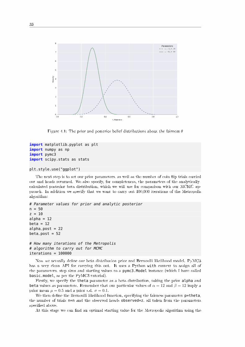
33

Figure 4.1: The prior and posterior belief distributions about the fairness θ

import matplotlib.pyplot as pltimport numpy as npimport pymc3import scipy.stats as stats

plt.style.use("ggplot")

The next step is to set our prior parameters, as well as the number of coin �ip trials carriedout and heads returned. We also specify, for completeness, the parameters of the analytically-calculated posterior beta distribution, which we will use for comparison with our MCMC ap-proach. In addition we specify that we want to carry out 100,000 iterations of the Metropolisalgorithm:

# Parameter values for prior and analytic posteriorn = 50z = 10alpha = 12beta = 12alpha_post = 22beta_post = 52

# How many iterations of the Metropolis# algorithm to carry out for MCMCiterations = 100000

Now we actually de�ne our beta distribution prior and Bernoulli likelihood model. PyMC3has a very clean API for carrying this out. It uses a Python with context to assign all ofthe parameters, step sizes and starting values to a pymc3.Model instance (which I have calledbasic_model, as per the PyMC3 tutorial).

Firstly, we specify the theta parameter as a beta distribution, taking the prior alpha andbeta values as parameters. Remember that our particular values of α = 12 and β = 12 imply aprior mean µ = 0.5 and a prior s.d. σ = 0.1.

We then de�ne the Bernoulli likelihood function, specifying the fairness parameter p=theta,the number of trials n=n and the observed heads observed=z, all taken from the parametersspeci�ed above.

At this stage we can �nd an optimal starting value for the Metropolis algorithm using the

34

PyMC3 Maximum A Posteriori (MAP) optimisation (we will go into detail about this in laterchapters). Finally we specify the Metropolis sampler to be used and then actually sample(..)the results. These results are stored in the trace variable:

# Use PyMC3 to construct a model contextbasic_model = pymc3.Model()with basic_model:

# Define our prior belief about the fairness# of the coin using a Beta distributiontheta = pymc3.Beta("theta", alpha=alpha, beta=beta)

# Define the Bernoulli likelihood functiony = pymc3.Binomial("y", n=n, p=theta, observed=z)

# Carry out the MCMC analysis using the Metropolis algorithm# Use Maximum A Posteriori (MAP) optimisation as initial value for MCMCstart = pymc3.find_MAP()

# Use the Metropolis algorithm (as opposed to NUTS or HMC, etc.)step = pymc3.Metropolis()

# Calculate the tracetrace = pymc3.sample(iterations, step, start, random_seed=1, progressbar=True

)

Notice how the speci�cation of the model via the PyMC3 API is almost akin to the actualmathematical speci�cation of the model, with minimal "boilerplate" code. We will demonstratethe power of this API in later chapters when we come to specify some more complex models.

Now that the model has been speci�ed and sampled, we wish to plot the results. We cre-ate a histogram from the trace (the list of all accepted samples) of the MCMC sampling us-ing 50 bins. We then plot the analytic prior and posterior beta distributions using the SciPystats.beta.pdf(..) method. Finally, we add some labelling to the graph and display it:

# Plot the posterior histogram from MCMC analysisbins=50plt.hist(

trace["theta"], bins,histtype="step", normed=True,label="Posterior (MCMC)", color="red"

)

# Plot the analytic prior and posterior beta distributionsx = np.linspace(0, 1, 100)plt.plot(

x, stats.beta.pdf(x, alpha, beta),"--", label="Prior", color="blue"

)plt.plot(

x, stats.beta.pdf(x, alpha_post, beta_post),label=’Posterior (Analytic)’, color="green"

)

# Update the graph labelsplt.legend(title="Parameters", loc="best")plt.xlabel("$\\theta$, Fairness")plt.ylabel("Density")plt.show()

35

When the code is executed the following output is given:

Applied logodds-transform to theta and added transformed theta_logodds tomodel.[----- 14% ] 14288 of 100000 complete in 0.5 sec[---------- 28% ] 28857 of 100000 complete in 1.0 sec[---------------- 43% ] 43444 of 100000 complete in 1.5 sec[-----------------58%-- ] 58052 of 100000 complete in 2.0 sec[-----------------72%------- ] 72651 of 100000 complete in 2.5 sec[-----------------87%------------- ] 87226 of 100000 complete in 3.0 sec[-----------------100%-----------------] 100000 of 100000 complete in 3.4 sec

Clearly, the sampling time will depend upon the speed of your computer. The graphicaloutput of the analysis is given in Figure 4.2:

Figure 4.2: Comparison of the analytic and MCMC-sampled posterior belief distributions aboutthe fairness θ, overlaid with the prior belief

In this particular case of a single-parameter model, with 100,000 samples, the convergenceof the Metropolis algorithm is extremely good. The histogram closely follows the analyticallycalculated posterior distribution, as we'd expect. In a relatively simple model such as this we donot need to compute 100,000 samples and far fewer would do. However, it does emphasise theconvergence of the Metropolis algorithm.

We can also consider a concept known as the trace, which is the vector of samples producedby the MCMC sampling procedure. We can use the helpful traceplot method to plot both akernel density estimate (KDE) of the histogram displayed above, as well as the trace.

The trace plot is extremely useful for assessing convergence of an MCMC algorithm andwhether we need to exclude a period of initial samples (known as the burn in). We will discussthe trace, burn in and other convergence issues in later sections when we study more sophisticatedsamplers. To output the trace we simply call traceplot with the trace variable:

# Show the trace plotpymc3.traceplot(trace)plt.show()

The full trace plot is given in Figure 4.3:

As you can see, the KDE estimate of the posterior belief in the fairness re�ects both our priorbelief of θ = 0.5 and our data with a sample fairness of θ = 0.2. In addition we can see that the

36

Figure 4.3: Trace plot of the MCMC sampling procedure for the fairness parameter θ

MCMC sampling procedure has "converged to the distribution" since the sampling series looksstationary.

In more complicated cases, which we will examine in later sections, we will see that we needto consider a "burn in" period as well as "thin" the results to remove autocorrelation, both ofwhich will improve convergence.

For completeness, here is the full listing:

import matplotlib.pyplot as pltimport numpy as npimport pymc3import scipy.stats as stats

plt.style.use("ggplot")

# Parameter values for prior and analytic posteriorn = 50z = 10alpha = 12beta = 12alpha_post = 22beta_post = 52

# How many iterations of the Metropolis# algorithm to carry out for MCMCiterations = 100000

# Use PyMC3 to construct a model contextbasic_model = pymc3.Model()with basic_model:

# Define our prior belief about the fairness# of the coin using a Beta distributiontheta = pymc3.Beta("theta", alpha=alpha, beta=beta)

37

# Define the Bernoulli likelihood functiony = pymc3.Binomial("y", n=n, p=theta, observed=z)

# Carry out the MCMC analysis using the Metropolis algorithm# Use Maximum A Posteriori (MAP) optimisation as initial value for MCMCstart = pymc3.find_MAP()

# Use the Metropolis algorithm (as opposed to NUTS or HMC, etc.)step = pymc3.Metropolis()

# Calculate the tracetrace = pymc3.sample(iterations, step, start, random_seed=1, progressbar=True

)

# Plot the posterior histogram from MCMC analysisbins=50plt.hist(

trace["theta"], bins,histtype="step", normed=True,label="Posterior (MCMC)", color="red"

)

# Plot the analytic prior and posterior beta distributionsx = np.linspace(0, 1, 100)plt.plot(

x, stats.beta.pdf(x, alpha, beta),"--", label="Prior", color="blue"

)plt.plot(

x, stats.beta.pdf(x, alpha_post, beta_post),label=’Posterior (Analytic)’, color="green"

)

# Update the graph labelsplt.legend(title="Parameters", loc="best")plt.xlabel("$\\theta$, Fairness")plt.ylabel("Density")plt.show()

# Show the trace plotpymc3.traceplot(trace)plt.show()

4.6 Next Steps

At this stage we have a good understanding of the basics behind MCMC, as well as a speci�cmethod known as the Metropolis algorithm, as applied to inferring a binomial proportion.

However, as we discussed above, PyMC3 uses a much more sophisticated MCMC samplerknown as the No-U-Turn Sampler (NUTS). In order to gain an understanding of this samplerwe eventually need to consider further sampling techniques such as Metropolis-Hastings, GibbsSampling and Hamiltonian Monte Carlo (on which NUTS is based).

We also want to start applying Probabilistic Programming techniques to more complex mod-els, such as hierarchical models. This in turn will help us produce sophisticated quantitative

38

trading strategies.

4.7 Bibliographic Note

The algorithm described in this chapter is due to Metropolis[36]. An improvement by Hastings[28]led to the Metropolis-Hastings algorithm. The Gibbs sampler is due to Geman and Geman[24].Gelfand and Smith[22] wrote a paper that was considered a major starting point for extensiveuse of MCMC methods in the statistical community.

The Hamiltonian Monte Carlo approach is due to Duane et al[20] and the No-U-Turn Sampler(NUTS) is due to Ho�man and Gelman[29]. Gelman et al[23] has an extensive discussion ofcomputional sampling mechanisms for Bayesian Statistics, including a detailed discussion onMCMC. A gentle, mathematically intuitive, introduction to the Metropolis Algorithm is givenby Kruschke[34].

A very popular on-line introduction to Bayesian Statistics is by Cam Davidson-Pilon andothers[19], which has a fantastic chapter on MCMC (and PyMC3). Thomas Wiecki has alsowritten a great blog post[50] explaining the rationale for MCMC.

The PyMC3 project[2] also has some extremely useful documentation and some examples.

Chapter 5

Bayesian Linear Regression

At this stage in our journey of Bayesian statistics we inferred a binomial proportion analyticallywith conjugate priors and have described the basics of Markov Chain Monte Carlo via theMetropolis algorithm. In this chapter we are going to introduce the basics of linear regressionmodelling in the Bayesian framework and carry out inference using the PyMC3 MCMC library.

We will begin by recapping the classical, or frequentist, approach to multiple linear regression(which will be discussed at length in the book part on Statistical Machine Learning in laterchapters). Then we will discuss how a Bayesian thinks of linear regression. We will brie�ydescribe the concept of a Generalised Linear Model (GLM), as this is necessary to understandthe clean syntax of model descriptions in PyMC3.

Subsequent to the description of these models we will simulate some linear data with noiseand then use PyMC3 to produce posterior distributions for the parameters of the model. Thisis the same procedure that we will carry out when discussing time series models such as ARMAand GARCH later on in the book. This "simulate and �t" process not only helps us understandthe model, but also checks that we are �tting it correctly when we know the "true" parametervalues.

Let's now turn our attention to the frequentist approach to linear regression.

5.1 Frequentist Linear Regression

The frequentist, or classical, approach to multiple linear regression assumes a model of theform[27]:

f (X) = β0 +

p∑j=1

Xjβj + ε = βTX + ε (5.1)

Where, βT is the transpose of the coe�cient vector β and ε ∼ N (0, σ2) is the measurementerror, normally distributed with mean zero and standard deviation σ.

That is, our model f(X) is linear in the predictors, X, with some associated measurementerror.

If we have a set of training data (x1, y1), . . . , (xN , yN ) then the goal is to estimate the βcoe�cients, which provide the best linear �t to the data. Geometrically, this means we need to�nd the orientation of the hyperplane that best linearly characterises the data.

"Best" in this case means minimising some form of error function. The most popular methodto do this is via ordinary least squares (OLS). If we de�ne the residual sum of squares (RSS),which is the sum of the squared di�erences between the outputs and the linear regression esti-mates:

39

40

RSS(β) =

N∑i=1

(yi − f(xi))2 (5.2)

=

N∑i=1

(yi − βTxi)2 (5.3)

Then the goal of OLS is to minimise the RSS, via adjustment of the β coe�cients. Althoughwe won't derive it here (see Hastie et al[27] for details) the Maximum Likelihood Estimate of β,which minimises the RSS, is given by:

β = (XTX)−1XTy (5.4)

To make a subsequent prediction yN+1, given some new data xN+1, we simply multiply thecomponents of xN+1 by the associated β coe�cients and obtain yN+1.

The important point here is that β is a point estimate. This means that it is a single valuein Rp+1. In the Bayesian formulation we will see that the interpretation di�ers substantially.

5.2 Bayesian Linear Regression

In a Bayesian framework, linear regression is stated in a probabilistic manner. That is, wereformulate the above linear regression model to use probability distributions. The syntax for alinear regression in a Bayesian framework looks like this:

y ∼ N(βTX, σ2I

)(5.5)

In words, our response datapoints y are sampled from a multivariate normal distribution thathas a mean equal to the product of the β coe�cients and the predictors, X, and a variance of σ2.Here, I refers to the identity matrix, which is necessary because the distribution is multivariate.

This is a very di�erent formulation to the frequentist approach. In the frequentist settingthere is no mention of probability distributions for anything other than the measurement error.In the Bayesian formulation the entire problem is recast such that the yi values are samples froma normal distribution.

A common question at this stage is "What is the bene�t of doing this?". What do we getout of this reformulation? There are two main reasons for doing so[?]:

� Prior Distributions: If we have any prior knowledge about the parameters β, then wecan choose prior distributions that re�ect this. If we don't, then we can still choose non-informative priors.

� Posterior Distributions: I mentioned above that the frequentist MLE value for ourregression coe�cients, β, was only a single point estimate. In the Bayesian formulation wereceive an entire probability distribution that characterises our uncertainty on the di�erentβ coe�cients. The immediate bene�t of this is that after taking into account any datawe can quantify our uncertainty in the β parameters via the variance of this posteriordistribution. A larger variance indicates more uncertainty.

While the above formula for the Bayesian approach may appear succinct, it doesn't reallygive us much clue as to how to specify a model and sample from it using Markov Chain MonteCarlo. In the next few sections we will use PyMC3 to formulate and utilise a Bayesian linearregression model.

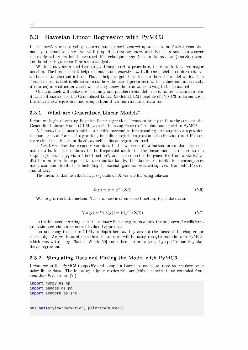
41

5.3 Bayesian Linear Regression with PyMC3

In this section we are going to carry out a time-honoured approach to statistical examples,namely to simulate some data with properties that we know, and then �t a model to recoverthese original properties. I have used this technique many times in the past on QuantStart.comand in later chapters on time series analysis.

While it may seem contrived to go through such a procedure, there are in fact two majorbene�ts. The �rst is that it helps us understand exactly how to �t the model. In order to do so,we have to understand it �rst. Thus it helps us gain intuition into how the model works. Thesecond reason is that it allows us to see how the model performs (i.e. the values and uncertaintyit returns) in a situation where we actually know the true values trying to be estimated.

Our approach will make use of numpy and pandas to simulate the data, use seaborn to plotit, and ultimately use the Generalised Linear Models (GLM) module of PyMC3 to formulate aBayesian linear regression and sample from it, on our simulated data set.

5.3.1 What are Generalised Linear Models?

Before we begin discussing Bayesian linear regression, I want to brie�y outline the concept of aGeneralised Linear Model (GLM), as we'll be using these to formulate our model in PyMC3.

A Generalised Linear Model is a �exible mechanism for extending ordinary linear regressionto more general forms of regression, including logistic regression (classi�cation) and Poissonregression (used for count data), as well as linear regression itself.

<P>GLMs allow for response variables that have error distributions other than the nor-mal distribution (see ε above, in the frequentist section). The linear model is related to theresponse/outcome, y, via a "link function", and is assumed to be generated from a statisticaldistribution from the exponential distribution family. This family of distributions encompassesmany common distributions including the normal, gamma, beta, chi-squared, Bernoulli, Poissonand others.

The mean of this distribution, µ depends on X via the following relation:

E(y) = µ = g−1(Xβ) (5.6)

Where g is the link function. The variance is often some function, V , of the mean:

Var(y) = V (E(y)) = V (g−1(Xβ)) (5.7)

In the frequentist setting, as with ordinary linear regression above, the unknown β coe�cientsare estimated via a maximum likelihood approach.

I'm not going to discuss GLMs in depth here as they are not the focus of the chapter (orthe book). We are interested in them because we will be using the glm module from PyMC3,which was written by Thomas Wiecki[50] and others, in order to easily specify our Bayesianlinear regression.

5.3.2 Simulating Data and Fitting the Model with PyMC3

Before we utilise PyMC3 to specify and sample a Bayesian model, we need to simulate somenoisy linear data. The following snippet carries this out (this is modi�ed and extended fromJonathan Sedar's post[?]):

import numpy as npimport pandas as pdimport seaborn as sns

sns.set(style="darkgrid", palette="muted")

42

def simulate_linear_data(N, beta_0, beta_1, eps_sigma_sq):"""Simulate a random dataset using a noisylinear process.

N: Number of data points to simulatebeta_0: Interceptbeta_1: Slope of univariate predictor, X"""# Create a pandas DataFrame with column ’x’ containing# N uniformly sampled values between 0.0 and 1.0df = pd.DataFrame(

{"x":np.random.RandomState(42).choice(

map(lambda x: float(x)/100.0,np.arange(100)

), N, replace=False)

})

# Use a linear model (y ~ beta_0 + beta_1*x + epsilon) to# generate a column ’y’ of responses based on ’x’eps_mean = 0.0df["y"] = beta_0 + beta_1*df["x"] + np.random.RandomState(42).normal(

eps_mean, eps_sigma_sq, N)

return df

if __name__ == "__main__":# These are our "true" parametersbeta_0 = 1.0 # Interceptbeta_1 = 2.0 # Slope

# Simulate 100 data points, with a variance of 0.5N = 100eps_sigma_sq = 0.5

# Simulate the "linear" data using the above parametersdf = simulate_linear_data(N, beta_0, beta_1, eps_sigma_sq)

# Plot the data, and a frequentist linear regression fit# using the seaborn packagesns.lmplot(x="x", y="y", data=df, size=10)plt.xlim(0.0, 1.0)

The output is given in Figure 5.1:We've simulated 100 datapoints, with an intercept β0 = 1 and a slope of β1 = 2. The epsilon

values are normally distributed with a mean of zero and variance σ2 = 12 . The data has been

plotted using the sns.lmplotmethod. In addition, the method uses a frequentist MLE approachto �t a linear regression line to the data.

Now that we have carried out the simulation we want to �t a Bayesian linear regression tothe data. This is where the glm module comes in. It uses a model speci�cation syntax that is

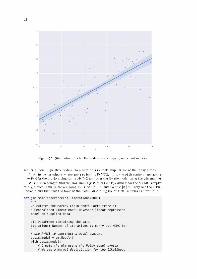
43

Figure 5.1: Simulation of noisy linear data via Numpy, pandas and seaborn

similar to how R speci�es models. To achieve this we make implicit use of the Patsy library.

In the following snippet we are going to import PyMC3, utilise the with context manager, asdescribed in the previous chapter on MCMC and then specify the model using the glm module.

We are then going to �nd the maximum a posteriori (MAP) estimate for the MCMC samplerto begin from. Finally, we are going to use the No-U-Turn Sampler[29] to carry out the actualinference and then plot the trace of the model, discarding the �rst 500 samples as "burn in":

def glm_mcmc_inference(df, iterations=5000):"""Calculates the Markov Chain Monte Carlo trace ofa Generalised Linear Model Bayesian linear regressionmodel on supplied data.

df: DataFrame containing the dataiterations: Number of iterations to carry out MCMC for"""# Use PyMC3 to construct a model contextbasic_model = pm.Model()with basic_model:

# Create the glm using the Patsy model syntax# We use a Normal distribution for the likelihood

44

pm.glm.glm("y ~ x", df, family=pm.glm.families.Normal())

# Use Maximum A Posteriori (MAP) optimisation# as initial value for MCMCstart = pm.find_MAP()

# Use the No-U-Turn Samplerstep = pm.NUTS()

# Calculate the tracetrace = pm.sample(

iterations, step, start,random_seed=42, progressbar=True

)

return trace

...

...

if __name__ == "__main__":......trace = glm_mcmc_inference(df, iterations=5000)pm.traceplot(trace[500:])plt.show()

The output of the script is as follows:

Applied log-transform to sd and added transformed sd_log to model.[---- 11% ] 563 of 5000 complete in 0.5 sec[--------- 24% ] 1207 of 5000 complete in 1.0 sec[-------------- 37% ] 1875 of 5000 complete in 1.5 sec[-----------------51% ] 2561 of 5000 complete in 2.0 sec[-----------------64%---- ] 3228 of 5000 complete in 2.5 sec[-----------------78%--------- ] 3920 of 5000 complete in 3.0 sec[-----------------91%-------------- ] 4595 of 5000 complete in 3.5 sec[-----------------100%-----------------] 5000 of 5000 complete in 3.8 sec

The traceplot is given in Figure 5.2:

We covered the basics of traceplots in the previous chapter. Recall that Bayesian modelsprovide a full posterior probability distribution for each of the model parameters, as opposed toa frequentist point estimate.

On the left side of the panel we can see marginal distributions for each parameter of interest.Notice that the intercept β0 distribution has its mode/maximum posterior estimate almost ex-actly at 1, close to the true parameter of β0 = 1. The estimate for the slope β1 parameter has amode at approximately 1.98, close to the true parameter value of β1 = 2. The ε error parameterassociated with the model measurement noise has a mode of approximately 0.465, which is alittle o� compared to the true value of ε = 0.5.

In all cases there is a reasonable variance associated with each marginal posterior, telling usthat there is some degree of uncertainty in each of the values. Were we to simulate more data,and carry out more samples, this variance would likely decrease.

The key point here is that we do not receive a single point estimate for a regression line, i.e."a line of best �t", as in the frequentist case. Instead we receive a distribution of likely regressionlines.

We can plot these lines using a method of the glm library called plot_posterior_predictive.The method takes a trace object and the number of lines to plot (samples).

45

Figure 5.2: Using PyMC3 to �t a Bayesian GLM linear regression model to simulated data

Firstly we use the seaborn lmplot method, this time with the fit_reg parameter set toFalse to stop the frequentist regression line being drawn. Then we plot 100 sampled posteriorpredictive regression lines. Finally, we plot the "true" regression line using the original β0 = 1and β1 = 2 parameters. The code snippet below produces such a plot:

..

..

if __name__ == "__main__":....

# Plot a sample of posterior regression linessns.lmplot(x="x", y="y", data=df, size=10, fit_reg=False)plt.xlim(0.0, 1.0)plt.ylim(0.0, 4.0)pm.glm.plot_posterior_predictive(trace, samples=100)x = np.linspace(0, 1, N)y = beta_0 + beta_1*xplt.plot(x, y, label="True Regression Line", lw=3., c="green")plt.legend(loc=0)plt.show()

We can see the sampled range of posterior regression lines in Figure 5.3:The main takeaway here is that there is uncertainty in the location of the regression line as

sampled by the Bayesian model. However, it can be seen that the range is relatively narrow andthat the set of samples is not too dissimilar to the "true" regression line itself.

5.4 Next Steps

The next step is to begin discussion of robust regression and hierarchical linear models, a powerfulmodelling technique made tractable by rapid MCMC implementations. From a quantitative

46

Figure 5.3: Using PyMC3 GLM module to show a set of sampled posterior regression lines

�nance point of view we will also take a look at a stochastic volatility model using PyMC3 andsee how we can use this model to form trading algorithms.

5.5 Bibliographic Note

An introduction to frequentist linear regression can be found in James et al[32]. A more technicaloverview, including subset selection methods, can be found in Hastie et al[27]. Gelman et al[23]discuss Bayesian linear models in depth at a reasonably technical level.

This chapter is in�uenced from previous blog posts by Thomas Wiecki[50] including hisdiscussion of Bayesian GLMs[48, 49] as well as Jonathan Sedar with his posts on BayesianInference with PyMC3[44].

5.6 Full Code

import matplotlib.pyplot as pltimport numpy as npimport pandas as pdimport pymc3 as pmimport seaborn as sns

47

sns.set(style="darkgrid", palette="muted")

def simulate_linear_data(N, beta_0, beta_1, eps_sigma_sq):"""Simulate a random dataset using a noisylinear process.

N: Number of data points to simulatebeta_0: Interceptbeta_1: Slope of univariate predictor, X"""# Create a pandas DataFrame with column ’x’ containing# N uniformly sampled values between 0.0 and 1.0df = pd.DataFrame(

{"x":np.random.RandomState(42).choice(

map(lambda x: float(x)/100.0,np.arange(N)

), N, replace=False)

})

# Use a linear model (y ~ beta_0 + beta_1*x + epsilon) to# generate a column ’y’ of responses based on ’x’eps_mean = 0.0df["y"] = beta_0 + beta_1*df["x"] + np.random.RandomState(42).normal(

eps_mean, eps_sigma_sq, N)

return df

def glm_mcmc_inference(df, iterations=5000):"""Calculates the Markov Chain Monte Carlo trace ofa Generalised Linear Model Bayesian linear regressionmodel on supplied data.

df: DataFrame containing the dataiterations: Number of iterations to carry out MCMC for"""# Use PyMC3 to construct a model contextbasic_model = pm.Model()with basic_model:

# Create the glm using the Patsy model syntax# We use a Normal distribution for the likelihoodpm.glm.glm("y ~ x", df, family=pm.glm.families.Normal())

# Use Maximum A Posteriori (MAP) optimisation# as initial value for MCMCstart = pm.find_MAP()

48

# Use the No-U-Turn Samplerstep = pm.NUTS()

# Calculate the tracetrace = pm.sample(

iterations, step, start,random_seed=42, progressbar=True

)

return trace

if __name__ == "__main__":# These are our "true" parametersbeta_0 = 1.0 # Interceptbeta_1 = 2.0 # Slope

# Simulate 100 data points, with a variance of 0.5N = 200eps_sigma_sq = 0.5

# Simulate the "linear" data using the above parametersdf = simulate_linear_data(N, beta_0, beta_1, eps_sigma_sq)

# Plot the data, and a frequentist linear regression fit# using the seaborn packagesns.lmplot(x="x", y="y", data=df, size=10)plt.xlim(0.0, 1.0)

trace = glm_mcmc_inference(df, iterations=5000)pm.traceplot(trace[500:])plt.show()

# Plot a sample of posterior regression linessns.lmplot(x="x", y="y", data=df, size=10, fit_reg=False)plt.xlim(0.0, 1.0)plt.ylim(0.0, 4.0)pm.glm.plot_posterior_predictive(trace, samples=100)x = np.linspace(0, 1, N)y = beta_0 + beta_1*xplt.plot(x, y, label="True Regression Line", lw=3., c="green")plt.legend(loc=0)plt.show()

Part III

Time Series Analysis

49

Chapter 6

Introduction to Time Series Analysis

In this chapter we are going to introduce methods from the �eld of time series analysis. Thesetechniques are extremely important in quantitative �nance as the vast majority of asset modellingin the �nancial industry still makes extensive use of these statistical models.

We will now examine what time series analysis is, outline its scope and learn how we canapply the techniques to various frequencies of �nancial data in order to predict future values orinfer relationships, ultimately allowing us to develop quantitative trading strategies.

6.1 What is Time Series Analysis?

Firstly, a time series is de�ned as some quantity that is measured sequentially in time oversome interval.

In its broadest form, time series analysis is about inferring what has happened to a series ofdata points in the past and attempting to predict what will happen to it in the future.

However, we are going to take a quantitative statistical approach to time series, by assumingthat our time series are realisations of sequences of random variables. That is, we are going toassume that there is some underlying generating process for our time series based on one or morestatistical distributions from which these variables are drawn.

Time series analysis attempts to understand the past and predict the future.

Such a sequence of random variables is known as a discrete-time stochastic process(DTSP). In quantitative trading we are concerned with attempting to �t statistical models tothese DTSPs to infer underlying relationships between series or predict future values in order togenerate trading signals.

Time series in general, including those outside of the �nancial world, often contain the fol-lowing features:

� Trends - A trend is a consistent directional movement in a time series. These trendswill either be deterministic or stochastic. The former allows us to provide an underlyingrationale for the trend, while the latter is a random feature of a series that we will beunlikely to explain. Trends often appear in �nancial series, particularly commodities prices,and many Commodity Trading Advisor (CTA) funds use sophisticated trend identi�cationmodels in their trading algorithms.

� Seasonal Variation - Many time series contain seasonal variation. This is particularlytrue in series representing business sales or climate levels. In quantitative �nance we oftensee seasonal variation in commodities, particularly those related to growing seasons orannual temperature variation (such as natural gas).

� Serial Dependence - One of the most important characteristics of time series, particularly�nancial series, is that of serial correlation. This occurs when time series observations thatare close together in time tend to be correlated. Volatility clustering is one aspect of serialcorrelation that is particularly important in quantitative trading.

51

52

6.2 How Can We Apply Time Series Analysis in Quantita-tive Finance?

Our goal as quantitative researchers is to identify trends, seasonal variations and correlationusing statistical time series methods, and ultimately generate trading signals or �lters based oninference or predictions.

Our approach will be to:

� Forecast and Predict Future Values - In order to trade successfully we will need toaccurately forecast future asset prices, at least in a statistical sense.

� Simulate Series - Once we identify statistical properties of �nancial time series we can usethem to generate simulations of future scenarios. This allows us to estimate the number oftrades, the expected trading costs, the expected returns pro�le, the technical and �nancialinvestment required in infrastructure, and thus ultimately the risk pro�le and pro�tabilityof a particular strategy or portfolio.

� Infer Relationships - Identi�cation of relationships between time series and other quan-titative values allows us to enhance our trading signals through �ltration mechanisms. Forexample, if we can infer how the spread in a foreign exchange pair varies with bid/askvolume, then we can �lter any prospective trades that may occur in a period where weforecast a wide spread in order to reduce transaction costs.

In addition we can apply standard (classical/frequentist or Bayesian) statistical tests to ourtime series models in order to justify certain behaviours, such as regime change in equity markets.

6.3 Time Series Analysis Software

In my two previous books we made exclusive use of C++ and Python for our trading strategyimplementation and simulation. Both of these languages are "�rst class environments" for writingan entire trading stack. They contain many libraries and allow an end-to-end construction of atrading system solely within that language.

Unfortunately, C++ and Python do not possess extensive statistical libraries. This is one oftheir shortcomings. For this reason we will be using the R statistical environment as a meansof carrying out time series research. R is well-suited for the job due to the availability of timeseries libraries, statistical methods and straightforward plotting capabilities.

We will learn R in a problem-solving fashion, whereby new commands and syntax will beintroduced as needed. Fortunately, there are plenty of extremely useful tutorials for R availabileon the internet and I will point them out as we go through the sequence of time series analysischapters.

6.4 Time Series Analysis Roadmap

We have previously discussed Bayesian statistics and that it will form the basis of many of ourtime series and machine learning models. Eventually we will utilise Bayesian tools and machinelearning techniques in conjunction with the following time series methods in order to forecastprice level and direction, act as �lters and determine "regime change", that is, determine whenour time series have changed their underlying statistical behaviour.

Our time series roadmap is as follows. Each of the topics below will form its own chapter.Once we've examined these methods in depth, we will be in a position to create some sophisticatedmodern models for examining high-frequency data across di�erent markets.

� Time Series Introduction - This chapter outlines the area of time series analysis, itsscope and how it can be applied to �nancial data.

53

� Serial Correlation - An absolutely fundamental aspect of modeling time series is theconcept of serial correlation. We will de�ne it, visualise it and outline how it can be usedto �t time series models.

� Random Walks and White Noise - In this chapter we will look at two basic timeseries models that will form the basis of the more complicated linear and conditional het-eroskedastic models of later chapters.

� ARMA Models - We will consider linear autoregressive, moving average and combinedautoregressive moving average models as our �rst attempt at predicting asset price move-ments.

� ARIMA and GARCH Models - We will extend the ARMA model to use di�erencingand thus allowing them to be "integrated", leading to the ARIMA model. We will alsodiscuss non-stationary conditional heteroskedastic (volatility clustering) models.

� Multivariate Modeling - We have considered multivariate models in Successful Algorith-mic Trading, namely when we considered mean-reverting pairs of equities. In this chapterwe will more rigourously de�ne cointegration and look at further tests for it. We will alsoconsider vector autoregressive (VAR) models [not to be confused with Value-at-Risk!].

� State-Space Models - State Space Modelling borrows a long history of modern controltheory used in engineering in order to allow us to model time series with rapidly varyingparameters (such as the β slope variable between two cointegrated assets in a linear regres-sion). In particular, we will consider the famous Kalman Filter and the Hidden MarkovModel. This will be one of the major uses of Bayesian analysis in time series.

� Market Microstructure - We will consider high frequency trading and examine marketmicrostructure e�ects in detail, later applying our knowledge to high-frequency forex data.

6.5 How Does This Relate to Other Statistical Tools?

My goal with QuantStart has always been to try and outline the mathematical and statisticalframework for quantitative analysis and quantitative trading, from the basics through to themore advanced modern techniques.

In previous books we have spent the majority of the time on introductory and intermediatetechniques. However, we are now going to turn our attention towards recent advanced techniquesused in quantitative �rms.

This will not only help those who wish to gain a career in the industry, but it will also give thequantitative retail traders among you a much broader toolkit of methods, as well as a unifyingapproach to trading.

Having worked full-time in the industry previously, and now as a consultant to funds, Ican state with certainty that a substantial fraction of quantitative fund professionals use verysophisticated techniques to "hunt for alpha".

However, many of these �rms are so large that they are not interested in "capacity con-strained" strategies, i.e. those that aren't scalable above 1-2million USD. As retailers, if wecan apply a sophisticated trading framework to these areas, coupled with a robust portfoliomanagement system and brokerage link, we can achieve pro�tability over the long term.

We will eventually combine our chapters on time series analysis with the Bayesian approachto hypothesis testing and model selection, along with optimised R and Python code, to producenon-linear, non-stationary time series models that can trade at high-frequency.

The next chapter will discuss serial correlation and why it is one of the most fundamentalaspects of time series analysis.

54

Chapter 7

Serial Correlation

In the previous chapter we considered how time series analysis models could be used to eventuallyallow us create trading strategies. In this chapter we are going to look at one of the mostimportant aspects of time series, namely serial correlation (also known as autocorrelation).

Before we dive into the de�nition of serial correlation we will discuss the broad purpose oftime series modelling and why we're interested in serial correlation.

When we are given one or more �nancial time series we are primarily interested in forecastingor simulating data. It is relatively straightforward to identify deterministic trends as well asseasonal variation and decompose a series into these components. However, once such a timeseries has been decomposed we are left with a random component.

Sometimes such a time series can be well modelled by independent random variables. How-ever, there are many situations, particularly in �nance, where consecutive elements of this randomcomponent time series will possess correlation. That is, the behaviour of sequential points in theremaining series a�ect each other in a dependent manner. One major example occurs in mean-reverting pairs trading. Mean-reversion shows up as correlation between sequential variables intime series.

Our task as quantitative modellers is to try and identify the structure of these correlations,as they will allow us to markedly improve our forecasts and thus the potential pro�tabilityof a strategy. In addition identifying the correlation structure will improve the realism of anysimulated time series based on the model. This is extremely useful for improving the e�ectivenessof risk management components of the strategy implementation.

When sequential observations of a time series are correlated in the manner described abovewe say that serial correlation (or autocorrelation) exists in the time series.

Now that we have outlined the usefulness of studying serial correlation we need to de�ne itin a rigourous mathematical manner. Before we can do that we must build on simpler concepts,including expectation and variance.

7.1 Expectation, Variance and Covariance

Many of these de�nitions will be familiar if you have a background in statistics or probability,but they will be outlined here speci�cally for purposes of consistent notation.

The �rst de�nition is that of the expected value or expectation:

De�nition 7.1.1. Expectation. The expected value or expectation, E(x), of a random variablex is its mean average value in the population. We denote the expectation of x by µ, such thatE(x) = µ.

Now that we have the de�nition of expectation we can de�ne the variance, which charac-terises the "spread" of a random variable:

De�nition 7.1.2. Variance. The variance of a random variable is the expectation of the squareddeviations of the variable from the mean, denoted by σ2(x) = E[(x− µ)2].

55

56

Notice that the variance is always non-negative. This allows us to de�ne the standard devia-tion:

De�nition 7.1.3. Standard Deviation. The standard deviation of a random variable x, σ(x), isthe square root of the variance of x.

Now that we've outlined these elementary statistical de�nitions we can generalise the varianceto the concept of covariance between two random variables. Covariance tells us how linearlyrelated these two variables are:

De�nition 7.1.4. Covariance. The covariance of two random variables x and y, each havingrespective expectations µx and µy, is given by σ(x, y) = E[(x− µx)(y − µy)].

Covariance tells us how two variables move together.

However since we are in a statistical situation we do not have access to the population meansµx and µy. Instead we must estimate the covariance from a sample. For this we use the respectivesample means x and y.

If we consider a set of n pairs of elements of random variables from x and y, given by (xi, yi),the sample covariance, Cov(x, y) (also sometimes denoted by q(x, y)) is given by:

Cov(x, y) =1

n− 1

n∑i=1

(xi − x)(yi − y) (7.1)

Note: You may be wondering why we divide by n−1 in the denominator, rather than n. Thisis a valid question! The reason we choose n−1 is that it makes Cov(x, y) an unbiased estimator.

7.1.1 Example: Sample Covariance in R

This is actually our �rst usage of R in the book. We have previously discussed the installationprocedure, so you can refer back to the introductory chapter if you need to install R. Assumingyou have R installed you can open up the R terminal.

In the following commands we are going to simulate two vectors of length 100, each with alinearly increasing sequence of integers with some normally distributed noise added. Thus weare constructing linearly associated variables by design.

We will �rstly construct a scatter plot and then calculate the sample covariance using thecor function. In order to ensure you see exactly the same data as I do, we will set a randomseed of 1 and 2 respectively for each variable:

> set.seed(1)> x <- seq(1,100) + 20.0*rnorm(1:100)> set.seed(2)> y <- seq(1,100) + 20.0*rnorm(1:100)> plot(x,y)

The plot is given in Figure 7.1.

There is a relatively clear association between the two variables. We can now calculate thesample covariance:

> cov(x,y)[1] 681.6859

The sample covariance is given as 681.6859.

One drawback of using the covariance to estimate linear association between two randomvariables is that it is a dimensional measure. That is, it isn't normalised by the spread of thedata and thus it is hard to draw comparisons between datasets with large di�erences in spread.This motivates another concept, namely correlation.

57

Figure 7.1: Scatter plot of two linearly increasing variables with normally distributed noise.

7.2 Correlation

Correlation is a dimensionless measure of how two variables vary together, or "co-vary". Inessence, it is the covariance of two random variables normalised by their respective spreads. The(population) correlation between two variables is often denoted by ρ(x, y):

ρ(x, y) =E[(x− µx)(y − µy)]

σxσy=σ(x, y)

σxσy(7.2)

The denominator product of the two spreads will constrain the correlation to lie within theinterval [−1, 1]:

� A correlation of ρ(x, y) = +1 indicates exact positive linear association

� A correlation of ρ(x, y) = 0 indicates no linear association at all

� A correlation of ρ(x, y) = −1 indicates exact negative linear association

As with the covariance, we can de�ne the sample correlation, Cor(x, y):

Cor(x, y) =Cov(x,y)

sd(x)sd(y)(7.3)

58

Where Cov(x, y) is the sample covariance of x and y, while sd(x) is the sample standarddeviation of x.

7.2.1 Example: Sample Correlation in R

We will use the same x and y vectors of the previous example. The following R code will calculatethe sample correlation:

> cor(x,y)[1] 0.5796604

The sample correlation is given as 0.5796604 showing a reasonably strong positive linearassociation between the two vectors, as expected.

7.3 Stationarity in Time Series

Now that we have outlined the de�nitions of expectation, variance, standard deviation, covarianceand correlation we are in a position to discuss how they apply to time series data.

Firstly, we will discuss a concept known as stationarity. This is an extremely importantaspect of time series and much of the analysis carried out on �nancial time series data willconcern stationarity. Once we have discussed stationarity we are in a position to talk aboutserial correlation and construct some correlogram plots.

We will begin by trying to apply the above de�nitions to time series data, starting with themean/expectation:

De�nition 7.3.1. Mean of a Time Series. The mean of a time series xt, µ(t), is given as theexpectation E(xt) = µ(t).

There are two important points to note about this de�nition:

� µ = µ(t), i.e. the mean (in general) is a function of time.

� This expectation is taken across the ensemble population of all the possible time seriesthat could have been generated under the time series model. In particular, it is NOT theexpression (x1 + x2 + ...+ xk)/k (more on this below).

This de�nition is useful when we are able to generate many realisations of a time series model.However in real life this is usually not the case! We are "stuck" with only one past history andas such we will often only have access to a single historical time series for a particular asset orsituation.

So how do we proceed if we wish to estimate the mean, given that we don't have access tothese hypothetical realisations from the ensemble? Well, there are two options:

� Simply estimate the mean at each point using the observed value.

� Decompose the time series to remove any deterministic trends or seasonality e�ects, givinga residual series. Once we have this series we can make the assumption that the residualseries is stationary in the mean, i.e. that µ(t) = µ, a �xed value independent of time. Itthen becomes possible to estimate this constant population mean using the sample meanx =

∑nt=1

xt

n .

De�nition 7.3.2. Stationary in the Mean. A time series is stationary in the mean if µ(t) = µ,a constant.

Now that we've seen how we can discuss expectation values we can use this to �esh out thede�nition of variance. Once again we make the simplifying assumption that the time series underconsideration is stationary in the mean. With that assumption we can de�ne the variance:

De�nition 7.3.3. Variance of a Time Series. The variance σ2(t) of a time series model that isstationary in the mean is given by σ2(t) = E[(xt − µ)2].

59

This is a straightforward extension of the variance de�ned above for random variables, exceptthat σ2(t) is a function of time. Importantly, you can see how the de�nition strongly relies onthe fact that the time series is stationary in the mean (i.e. that µ is not time-dependent).

You might notice that this de�nition leads to a tricky situation. If the variance itself varieswith time how are we supposed to estimate it from a single time series? As before, the presenceof the expectation operator E(..) requires an ensemble of time series and yet we will often onlyhave one!

Once again, we simplify the situation by making an assumption. In particular, and as withthe mean, we assume a constant population variance, denoted σ2, which is not a function oftime. Once we have made this assumption we are in a position to estimate its value using thesample variance de�nition above:

Var(x) =

∑(xt − x)2

n− 1(7.4)

Note for this to work we need to be able to estimate the sample mean, x. In addition, as withthe sample covariance de�ned above, we must use n− 1 in the denominator in order to make thesample variance an unbiased estimator.

De�nition 7.3.4. Stationary in the Variance. A time series is stationary in the variance ifσ2(t) = σ2, a constant.

This is where we need to be careful! With time series we are in a situation where sequentialobservations may be correlated. This will have the e�ect of biasing the estimator, i.e. over- orunder-estimating the true population variance.

This will be particularly problematic in time series where we are short on data and thus onlyhave a small number of observations. In a high correlation series, such observations will be closeto each other and thus will lead to bias.

In practice, and particularly in high-frequency �nance, we are often in a situation of having asubstantial number of observations. The drawback is that we often cannot assume that �nancialseries are truly stationary in the mean or stationary in the variance.

As we make progress with the section in the book on time series, and develop more sophisti-cated models, we will address these issues in order to improve our forecasts and simulations.

We are now in a position to apply our time series de�nitions of mean and variance to that ofserial correlation.

7.4 Serial Correlation

The essence of serial correlation is that we wish to see how sequential observations in a timeseries a�ect each other. If we can �nd structure in these observations then it will likely helpus improve our forecasts and simulation accuracy. This will lead to greater pro�tability in ourtrading strategies or better risk management approaches.

Firstly, another de�nition. If we assume, as above, that we have a time series that is stationaryin the mean and stationary in the variance then we can talk about second order stationarity:

De�nition 7.4.1. Second Order Stationary. A time series is second order stationary if thecorrelation between sequential observations is only a function of the lag, that is, the number oftime steps separating each sequential observation.

Finally, we are in a position to de�ne serial covariance and serial correlation!

De�nition 7.4.2. Autocovariance of a Time Series. If a time series model is second orderstationary then the (population) serial covariance or autocovariance, of lag k, Ck = E[(xt −µ)(xt+k − µ)].

The autocovariance Ck is not a function of time. This is because it involves an expectationE(..), which, as before, is taken across the population ensemble of possible time series realisations.This means it is the same for all times t.

60

As before this motivates the de�nition of serial correlation or autocorrelation, simply bydividing through by the square of the spread of the series. This is possible because the timeseries is stationary in the variance and thus σ2(t) = σ2:

De�nition 7.4.3. Autocorrelation of a Time Series. The serial correlation or autocorrelationof lag k, ρk, of a second order stationary time series is given by the autocovariance of the seriesnormalised by the product of the spread. That is, ρk = Ck

σ2 .

Note that ρ0 = C0

σ2 = E[(xt−µ)2]σ2 = σ2

σ2 = 1. That is, the �rst lag of k = 0 will always give avalue of unity.

As with the above de�nitions of covariance and correlation, we can de�ne the sample auto-covariance and sample autocorrelation. In particular, we denote the sample autocovariance witha lower-case c to di�erentiate between the population value given by an upper-case C.

The sample autocovariance function ck is given by:

ck =1

n

n−k∑t=1

(xt − x)(xt+k − x) (7.5)

The sample autocorrelation function rk is given by:

rk =ckc0

(7.6)

Now that we have de�ned the sample autocorrelation function we are in a position to de�neand plot the correlogram, an essential tool in time series analysis.

7.5 The Correlogram

A correlogram is simply a plot of the autocorrelation function for sequential values of lagk = 0, 1, ..., n. It allows us to see the correlation structure in each lag.

The main usage of correlograms is to detect any autocorrelation subsequent to the removalof any deterministic trends or seasonality e�ects.

If we have �tted a time series model then the correlogram helps us justify that this model iswell �tted or whether we need to further re�ne it to remove any additional autocorrelation.

Here is an example correlogram, plotted in R using the acf function, for a sequence ofnormally distributed random variables. The full R code is as follows and is plotted in Figure 7.2.

> set.seed(1)> w <- rnorm(100)> acf(w)

There are a few notable features of the correlogram plot in R:

� Firstly, since the sample correlation of lag k = 0 is given by r0 = c0c0

= 1 we will alwayshave a line of height equal to unity at lag k = 0 on the plot. In fact, this provides us witha reference point upon which to judge the remaining autocorrelations at subsequent lags.Note also that the y-axis ACF is dimensionless, since correlation is itself dimensionless.

� The dotted blue lines represent boundaries upon which if values fall outside of these, wehave evidence against the null hypothesis that our correlation at lag k, rk, is equal to zeroat the 5% level. However we must take care because we should expect 5% of these lags toexceed these values anyway! Further we are displaying correlated values and hence if one lagfalls outside of these boundaries then proximate sequential values are more likely to do so aswell. In practice we are looking for lags that may have some underlying reason for exceedingthe 5% level. For instance, in a commodity time series we may be seeing unanticipatedseasonality e�ects at certain lags (possibly monthly, quarterly or yearly intervals).

Here are a couple of examples of correlograms for sequences of data.

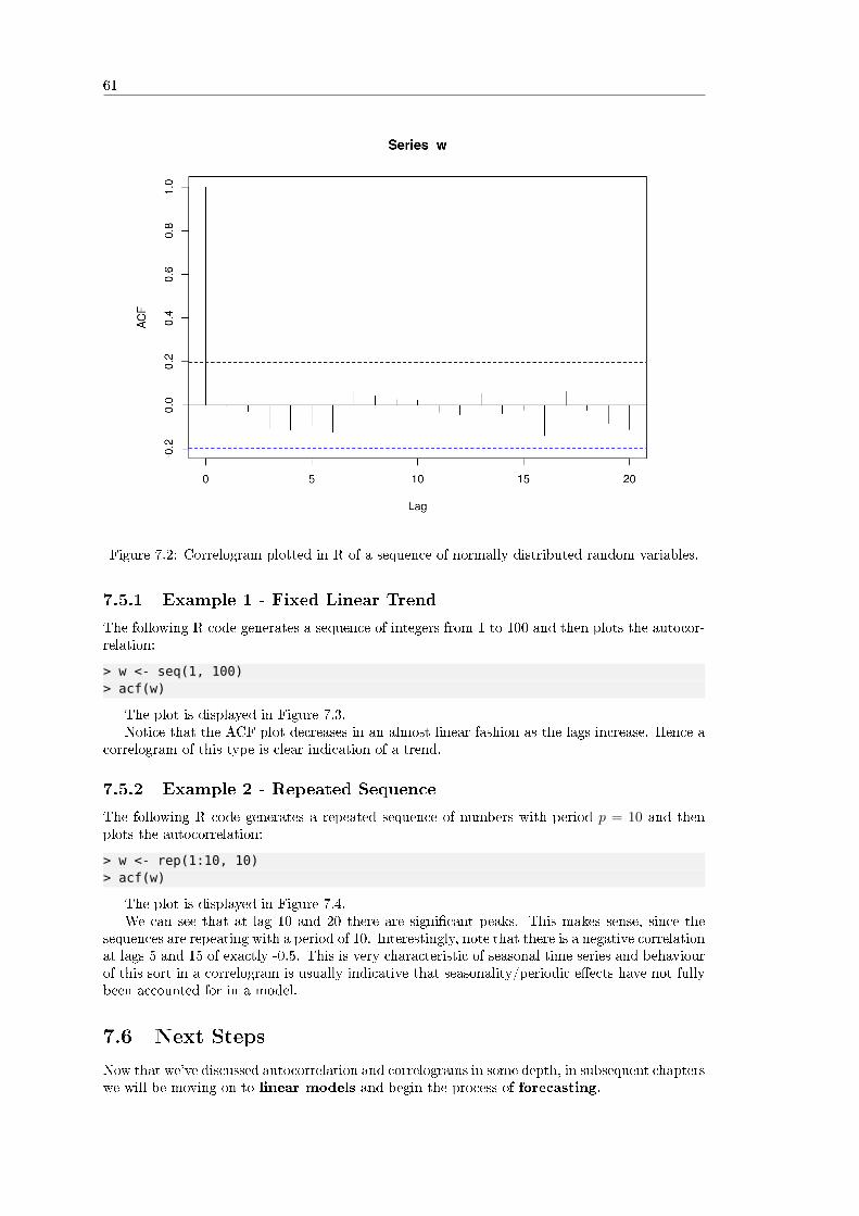
61

Figure 7.2: Correlogram plotted in R of a sequence of normally distributed random variables.

7.5.1 Example 1 - Fixed Linear Trend

The following R code generates a sequence of integers from 1 to 100 and then plots the autocor-relation:

> w <- seq(1, 100)> acf(w)

The plot is displayed in Figure 7.3.Notice that the ACF plot decreases in an almost linear fashion as the lags increase. Hence a

correlogram of this type is clear indication of a trend.

7.5.2 Example 2 - Repeated Sequence

The following R code generates a repeated sequence of numbers with period p = 10 and thenplots the autocorrelation:

> w <- rep(1:10, 10)> acf(w)

The plot is displayed in Figure 7.4.We can see that at lag 10 and 20 there are signi�cant peaks. This makes sense, since the

sequences are repeating with a period of 10. Interestingly, note that there is a negative correlationat lags 5 and 15 of exactly -0.5. This is very characteristic of seasonal time series and behaviourof this sort in a correlogram is usually indicative that seasonality/periodic e�ects have not fullybeen accounted for in a model.

7.6 Next Steps

Now that we've discussed autocorrelation and correlograms in some depth, in subsequent chapterswe will be moving on to linear models and begin the process of forecasting.

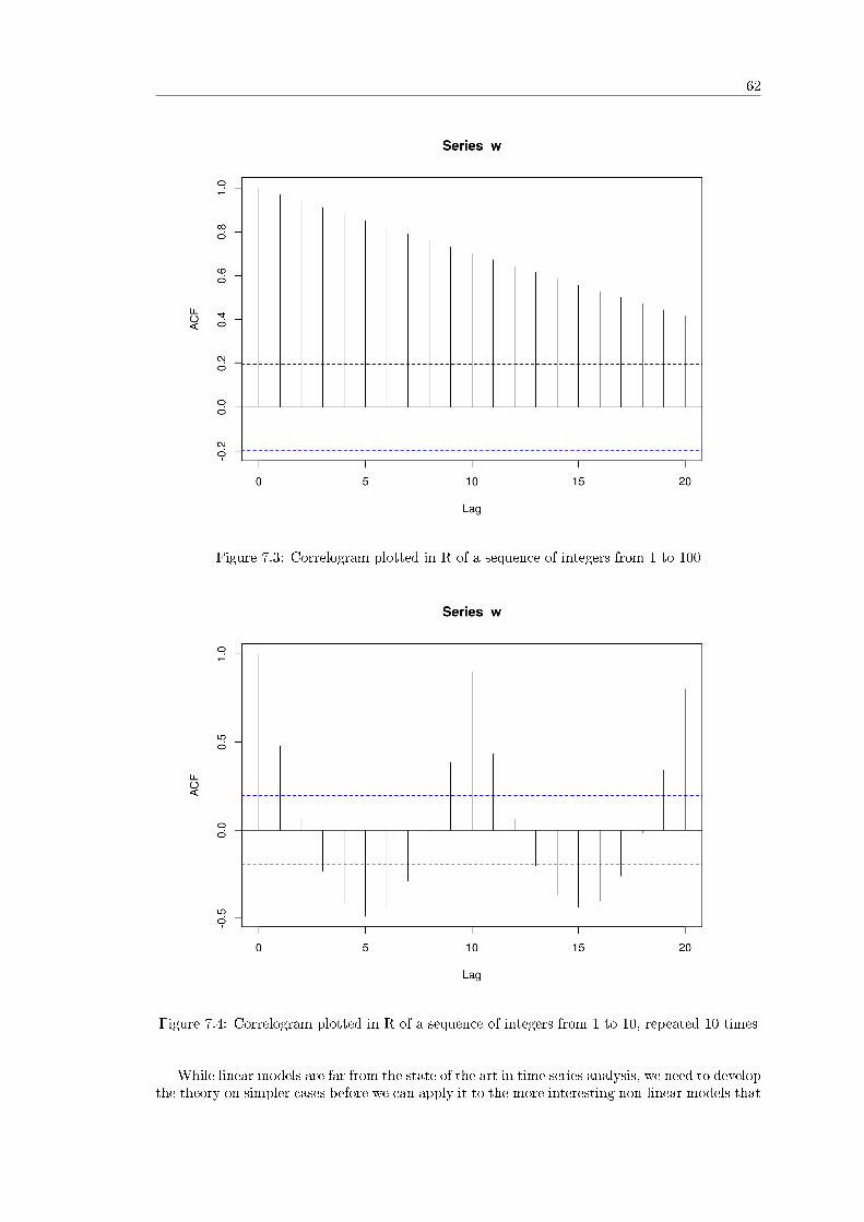
62

Figure 7.3: Correlogram plotted in R of a sequence of integers from 1 to 100

Figure 7.4: Correlogram plotted in R of a sequence of integers from 1 to 10, repeated 10 times

While linear models are far from the state of the art in time series analysis, we need to developthe theory on simpler cases before we can apply it to the more interesting non-linear models that

63

are in use today.

64

Chapter 8

Random Walks and White NoiseModels

In the previous chapter we discussed the importance of serial correlation and why it is ex-tremely useful in the context of quantitative trading.

In this chapter we will make full use of serial correlation by discussing our �rst time seriesmodels, including some elementary linear stochastic models. In particular we are going to discussthe White Noise and Random Walk models.

8.1 Time Series Modelling Process

What is a time series model? Essentially, it is a mathematical model that attempts to "explain"the serial correlation present in a time series.

When we say "explain" what we really mean is once we have "�tted" a model to a time seriesit should account for some or all of the serial correlation present in the correlogram. That is,by �tting the model to a historical time series, we are reducing the serial correlation and thus"explaining it away".

Our process, as quantitative researchers, is to consider a wide variety of models includingtheir assumptions and their complexity, and then choose a model such that it is the "simplest"that will explain the serial correlation. Once we have such a model we can use it to predictfuture values, or future behaviour in general. This prediction is obviously extremely useful inquantitative trading.

If we can predict the direction of an asset movement then we have the basis of a tradingstrategy (allowing for transaction costs, of course!). Also, if we can predict volatility of an assetthen we have the basis of another trading strategy or a risk-management approach. This is whywe are interested in second order properties, since they give us the means to help us makeforecasts.

How do we know when we have a good �t for a model? What criteria do we use to judgewhich model is best? We will be considering these questions in this part of the book.

Let's summarise the general process we will be following throughout the time series section:

� Outline a hypotheis about a particular time series and its behaviour

� Obtain the correlogram of the time series using R and assess its serial correlation

� Use our knowledge of time series to �t an appropriate model that reduces the serial corre-lation in the residuals

� Re�ne the �t until no correlation is present and then subsequently make use of statisticalgoodness-of-�t tests to assess the model �t

� Use the model and its second-order properties to make forecasts about future values

65

66

� Iterate through this process until the forecast accuracy is optimised

� Utilise such forecasts to create trading strategies

That is our basic process. The complexity will arise when we consider more advanced modelsthat account for additional serial correlation in our time series.

In this chapter we are going to consider two of the most basic time series models, namelyWhite Noise and Random Walks. These models will form the basis of more advanced modelslater so it is essential we understand them well.

However, before we introduce either of these models, we are going to discuss some moreabstract concepts that will help us unify our approach to time series models. In particular, weare going to de�ne the Backward Shift Operator and the Di�erence Operator.

8.2 Backward Shift and Di�erence Operators

The Backward Shift Operator (BSO) and the Di�erence Operator will allow us to writemany di�erent time series models in a particularly succinct way that more easily allows us todraw comparisons between them.

Since we will be using the notation of each so frequently, it makes sense to de�ne them now.

De�nition 8.2.1. Backward Shift Operator. The backward shift operator or lag operator, B,takes a time series element as an argument and returns the element one time unit previously:Bxt = xt−1.

Repeated application of the operator allows us to step back n times: Bnxt = xt−n.

We will use the BSO to de�ne many of our time series models going forward.In addition, when we come to study time series models that are non-stationary (that is, their

mean and variance can alter with time), we can use a di�erencing procedure in order to take anon-stationary series and produce a stationary series from it.

De�nition 8.2.2. Di�erence Operator. The di�erence operator,∇, takes a time series element asan argument and returns the di�erence between the element and that of one time unit previously:∇xt = xt − xt−1, or ∇xt = (1−B)xt.

As with the BSO, we can repeatedly apply the di�erence operator: ∇n = (1−B)n.

Now that we've discussed these abstract operators, let us consider some concrete time seriesmodels.

8.3 White Noise

Let's begin by trying to motivate the concept of White Noise.Above, we mentioned that our basic approach was to try �tting models to a time series until

the remaining series lacked any serial correlation. This motivates the de�nition of the residualerror series:

De�nition 8.3.1. Residual Error Series. The residual error series or residuals, xt, is a timeseries of the di�erence between an observed value and a predicted value, from a time series model,at a particular time t.

If yt is the observed value and yt is the predicted value, we say: xt = yt− yt are the residuals.

The key point is that if our chosen time series model is able to "explain" the serial corre-lation in the observations, then the residuals themselves are serially uncorrelated. This meansthat each element of the serially uncorrelated residual series is an independent realisation fromsome probability distribution. That is, the residuals themselves are independent and identicallydistributed (i.i.d.).

Hence, if we are to begin creating time series models that explain away any serial correlation,it seems natural to begin with a process that produces independent random variables from somedistribution. This directly leads on to the concept of (discrete) white noise:

67

De�nition 8.3.2. Discrete White Noise. Consider a time series {wt : t = 1, ...n}. If the elementsof the series, wi, are independent and identically distributed (i.i.d.), with a mean of zero, varianceσ2 and no serial correlation (i.e. Cor(wi, wj) = 0,∀i 6= j) then we say that the time series isdiscrete white noise (DWN).

In particular, if the values wi are drawn from a standard normal distribution (i.e. wt ∼N (0, σ2)), then the series is known as Gaussian White Noise.

White Noise is useful in many contexts. In particular, it can be used to simulate a syntheticseries.

As we've mentioned before, a historical time series is only one observed instance. If we cansimulate multiple realisations then we can create "many histories" and thus generate statisticsfor some of the parameters of particular models. This will help us re�ne our models and thusincrease accuracy in our forecasting.

Now that we've de�ned Discrete White Noise, we are going to examine some of the attributesof it, including its second order properties and its correlogram.

8.3.1 Second-Order Properties

The second-order properties of DWN are straightforward and follow easily from the actual de�-nition. In particular, the mean of the series is zero and there is no autocorrelation by de�nition:

µw = E(wt) = 0 (8.1)

ρk = Cor(wt, wt+k) =

{1 if k = 0

0 if k 6= 0

8.3.2 Correlogram

We can also plot the correlogram of a DWN using R, see Figure 8.1. Firstly we'll set the randomseed to be 1, so that your random draws will be identical to mine. Then we will sample 1000elements from a normal distribution and plot the autocorrelation:

> set.seed(1)> acf(rnorm(1000))

Notice that at k = 6, k = 15 and k = 18, we have three peaks that di�er from zero at the 5%level. However, this is to be expected simply due to the variation in sampling from the normaldistribution.

Once again, we must be extremely careful in our interpretation of results. In this instance,do we really expect anything physically meaningful to be happening at k = 6, k = 15 or k = 18?

Notice that the DWN model only has a single parameter, namely the variance σ2. Thankfully,it is straightforward to estimate the variance with R. We can simply use the var function:

> set.seed(1)> var(rnorm(1000, mean=0, sd=1))[1] 1.071051

We've speci�cally highlighted that the normal distribution above has a mean of zero and astandard deviation of 1 (and thus a variance of 1). R calculates the sample variance as 1.071051,which is close to the population value of 1.

The key takeaway with Discrete White Noise is that we use it as a model for the residuals.We are looking to �t other time series models to our observed series, at which point we use DWNas a con�rmation that we have eliminated any remaining serial correlation from the residualsand thus have a good model �t.

Now that we have examined DWN we are going to move on to a famous model for (some)�nancial time series, namely the Random Walk.

68

Figure 8.1: Correlogram of Discrete White Noise.

8.4 Random Walk.

A random walk is another time series model where the current observation is equal to theprevious observation with a random step up or down. It is formally de�ned below:

De�nition 8.4.1. Random Walk A random walk is a time series model xt such that xt =xt−1 + wt, where wt is a discrete white noise series.

Recall above that we de�ned the backward shift operator B. We can apply the BSO to therandom walk:

xt = Bxt + wt = xt−1 + wt (8.2)

And stepping back further:

xt−1 = Bxt−1 + wt−1 = xt−2 + wt−1 (8.3)

If we repeat this process until the end of the time series we get:

xt = (1 + B + B2 + . . .)wt =⇒ xt = wt + wt−1 + wt−2 + . . . (8.4)

Hence it is clear to see how the random walk is simply the sum of the elements from a discretewhite noise series.

8.4.1 Second-Order Properties

The second-order properties of a random walk are a little more interesting than that of discretewhite noise. While the mean of a random walk is still zero, the covariance is actually time-dependent. Hence a random walk is non-stationary:

69

µx = 0 (8.5)

γk(t) = Cov(xt, xt+k) = tσ2 (8.6)

In particular, the covariance is equal to the variance multiplied by the time. Hence, as timeincreases, so does the variance.

What does this mean for random walks? Put simply, it means there is very little point inextrapolating "trends" in them over the long term, as they are literally random walks.

8.4.2 Correlogram

The autocorrelation of a random walk (which is also time-dependent) can be derived as follows:

ρk(t) =Cov(xt, xt+k)√Var(xt)Var(xt+k)

=tσ2√

tσ2(t+ k)σ2=

1√1 + k/t

(8.7)

Notice that this implies if we are considering a long time series, with short term lags, thenwe get an autocorrelation that is almost unity. That is, we have extremely high autocorrelationthat does not decrease very rapidly as the lag increases. We can simulate such a series using R.

Firstly, we set the seed so that you can replicate my results exactly. Then we create twosequences of random draws (x and w), each of which has the same value (as de�ned by the seed).

We then loop through every element of x and assign it the value of the previous value ofx plus the current value of w. This gives us the random walk. We then plot the results usingtype="l" to give us a line plot, rather than a plot of circular points, see Figure 8.2.

> set.seed(4)> x <- w <- rnorm(1000)> for (t in 2:1000) x[t] <- x[t-1] + w[t]> plot(x, type="l")

It is simple enough to draw the correlogram too, see Figure 8.3.

> acf(x)

8.4.3 Fitting Random Walk Models to Financial Data

We mentioned above that we would try and �t models to data which we have already simulated.Clearly this is somewhat contrived, as we've simulated the random walk in the �rst place!

However, we're trying to demonstrate the �tting process. In real situations we won't knowthe underlying generating model for our data, we will only be able to �t models and thenassess the correlogram.

We stated that this process was useful because it helps us check that we've correctly imple-mented the model by trying to ensure that parameter estimates are close to those used in thesimulations.

Fitting to Simulated Data

Since we are going to be spending a lot of time �tting models to �nancial time series, we shouldget some practice on simulated data �rst, such that we're well-versed in the process once we startusing real data.

We have already simulated a random walk so we may as well use that realisation to see if ourproposed model (of a random walk) is accurate.

How can we tell if our proposed random walk model is a good �t for our simulated data?Well, we make use of the de�nition of a random walk, which is simply that the di�erence betweentwo neighbouring values is equal to a realisation from a discrete white noise process.

Hence, if we create a series of the di�erences of elements from our simulated series, we shouldhave a series that resembles discrete white noise!

70

Figure 8.2: Realisation of a Random Walk with 1000 timesteps.

Figure 8.3: Correlogram of a Random Walk.

In R this can be accomplished very straightforwardly using the diff function. Once we havecreated the di�erence series, we wish to plot the correlogram and then assess how close this is to

71

discrete white noise, see Figure 8.4.

> acf(diff(x))

Figure 8.4: Correlogram of the Di�erence Series from a Simulated Random Walk.

What can we notice from this plot? There is a statistically signi�cant peak at k = 10, but onlymarginally. Remember, that we expect to see at least 5% of the peaks be statistically signi�cant,simply due to sampling variation.

Hence we can reasonably state that the the correlogram looks like that of discrete white noise.It implies that the random walk model is a good �t for our simulated data. This is exactly whatwe should expect, since we simulated a random walk in the �rst place!

Fitting to Financial Data

Let's now apply our random walk model to some actual �nancial data. As with the Pythonlibrary pandas we can use the R package quantmod to easily extract �nancial data fromYahoo Finance.

We are going to see if a random walk model is a good �t for some equities data. In particular,I am going to choose Microsoft (MSFT), but you can experiment with your favourite tickersymbol.

Before we're able to download any of the data, we must install quantmod as it isn't part ofthe default R installation. Run the following command and select the R package mirror serverthat is closest to your location:

> install.packages(’quantmod’)

Once quantmod is installed we can use it to obtain the historical price of MSFT stock:

> require(’quantmod’)> getSymbols(’MSFT’, src=’yahoo’)> MSFT....

72

2015-07-15 45.68 45.89 45.43 45.76 26482000 45.760002015-07-16 46.01 46.69 45.97 46.66 25894400 46.660002015-07-17 46.55 46.78 46.26 46.62 29262900 46.62000

This will create an object called MSFT (case sensitive!) into the R namespace, which containsthe pricing and volume history of MSFT. We're interested in the corporate-action adjusted closingprice. We can use the following commands to (respectively) obtain the Open, High, Low, Close,Volume and Adjusted Close prices for the Microsoft stock: Op(MSFT), Hi(MSFT), Lo(MSFT),Cl(MSFT), Vo(MSFT), Ad(MSFT).

Our process will be to take the di�erence of the Adjusted Close values, omit any missingvalues, and then run them through the autocorrelation function. When we plot the correlogramwe are looking for evidence of discrete white noise, that is, a residuals series that is seriallyuncorrelated. To carry this out in R, we run the following command:

> acf(diff(Ad(MSFT)), na.action = na.omit)

The latter part (na.action = na.omit) tells the acf function to ignore missing values byomitting them. The output of the acf function is given in Figure 8.5.

Figure 8.5: Correlogram of the Di�erence Series from MSFT Adjusted Close.

We notice that the majority of the lag peaks do not di�er from zero at the 5% level. Howeverthere are a few that are marginally above. Given that the lags ki where peaks exist are somewayfrom k = 0, we could be inclined to think that these are due to stochastic variation and do notrepresent any physical serial correlation in the series.

Hence we can conclude, with a reasonable degree of certainty, that the adjusted closing pricesof MSFT are well approximated by a random walk.

Let's now try the same approach on the S&P500 itself. The Yahoo Finance symbol for theS&P500 index is ^GSPC. Hence, if we enter the following commands into R, we can plot thecorrelogram of the di�erence series of the S&P500:

> getSymbols(’^GSPC’, src=’yahoo’)> acf(diff(Ad(GSPC)), na.action = na.omit)

73

Figure 8.6: Correlogram of the Di�erence Series from the S&P500 Adjusted Close.

The correlogram is given in Figure 8.6.The correlogram here is certainly more interesting. Notice that there is a negative correlation

at k = 1. This is unlikely to be due to random sampling variation.Notice also that there are peaks at k = 15, k = 16 and k = 18. Although it is harder to

justify their existence beyond that of random variation, they may be indicative of a longer-lagprocess.

Hence it is much harder to justify that a random walk is a good model for the S&P500Adjusted Close data. This motivates more sophisticated models, namely the AutoregressiveModels of Order p, which will be the subject of the following chapter.

74

Chapter 9

Autoregressive Moving AverageModels

In the last chapter we looked at random walks and white noise as basic time series models forcertain �nancial instruments, such as daily equity and equity index prices. We found that insome cases a random walk model was insu�cient to capture the full autocorrelation behaviourof the instrument, which motivates more sophisticated models.

In this chapter we are going to discuss three types of model, namely the Autoregressive(AR) model of order p, the Moving Average (MA) model of order q and the mixed Auto-gressive Moving Average (ARMA) model of order p, q. These models will help us attemptto capture or "explain" more of the serial correlation present within an instrument. Ultimatelythey will provide us with a means of forecasting the future prices.

However, it is well known that �nancial time series possess a property known as volatilityclustering. That is, the volatility of the instrument is not constant in time. The technical termfor this behaviour is conditional heteroskedasticity. Since the AR, MA and ARMA modelsare not conditionally heteroskedastic, that is, they don't take into account volatility clustering,we will ultimately need a more sophisticated model for our predictions.

Such models include the Autogressive Conditional Heteroskedastic (ARCH) modeland Generalised Autogressive Conditional Heteroskedastic (GARCH) model, and themany variants thereof. GARCH is particularly well known in quant �nance and is primarily usedfor �nancial time series simulations as a means of estimating risk.

However, we will be building up to these models from simpler versions in order to see howeach new variant changes our predictive ability. Despite the fact that AR, MA and ARMA arerelatively simple time series models, they are the basis of more complicated models such as theAutoregressive Integrated Moving Average (ARIMA) and the GARCH family. Hence itis important that we study them.

One of our trading strategies later in the book will be to combine ARIMA and GARCH inorder to predict prices n periods in advance. However, we will have to wait until we've discussedboth ARIMA and GARCH separately before we apply them to this strategy.

9.1 How Will We Proceed?

In this chapter we are going to outline some new time series concepts that we'll need for the re-maining methods, namely strict stationarity and the Akaike information criterion (AIC).

Subsequent to these new concepts we will follow the traditional pattern for studying new timeseries models:

� Rationale - The �rst task is to provide a reason why we're interested in a particular model,as quants. Why are we introducing the time series model? What e�ects can it capture?What do we gain (or lose) by adding in extra complexity?

75

76

� De�nition - We need to provide the full mathematical de�nition (and associated notation)of the time series model in order to minimise any ambiguity.

� Second Order Properties - We will discuss (and in some cases derive) the second orderproperties of the time series model, which includes its mean, its variance and its autocor-relation function.

� Correlogram - We will use the second order properties to plot a correlogram of a realisa-tion of the time series model in order to visualise its behaviour.

� Simulation - We will simulate realisations of the time series model and then �t the modelto these simulations to ensure we have accurate implementations and understand the �ttingprocess.

� Real Financial Data - We will �t the time series model to real �nancial data and considerthe correlogram of the residuals in order to see how the model accounts for serial correlationin the original series.

� Prediction - We will create n-step ahead forecasts of the time series model for particularrealisations in order to ultimately produce trading signals.

Nearly all of the chapters written in this book on time series models will fall into this patternand it will allow us to easily compare the di�erences between each model as we add furthercomplexity.

We're going to start by looking at strict stationarity and the AIC.

9.2 Strictly Stationary

We provided the de�nition of stationarity in the chapter on serial correlation. However, becausewe are going to be entering the realm of many �nancial series, with various frequencies, we needto make sure that our (eventual) models take into account the time-varying volatility of theseseries. In particular, we need to consider their heteroskedasticity.

We will come across this issue when we try to �t certain models to historical series. Generally,not all of the serial correlation in the residuals of �tted models can be accounted for withouttaking heteroskedasticity into account. This brings us back to stationarity. A series is notstationary in the variance if it has time-varying volatility, by de�nition.

This motivates a more rigourous de�nition of stationarity, namely strict stationarity:

De�nition 9.2.1. Strictly Stationary Series. A time series model, {xt}, is strictly stationary ifthe joint statistical distribution of the elements xt1 , . . . , xtn is the same as that of xt1+m, . . . , xtn+m,∀ti,m.

One can think of this de�nition as simply that the distribution of the time series is unchangedfor any abritrary shift in time.

In particular, the mean and the variance are constant in time for a strictly stationary seriesand the autocovariance between xt and xs (say) depends only on the absolute di�erence of t ands, |t− s|.

We will be revisiting strictly stationary series in future chapters.

9.3 Akaike Information Criterion

I mentioned in previous chapters that we would eventually need to consider how to choose betweenseparate "best" models. This is true not only of time series analysis, but also of machine learningand, more broadly, statistics in general.

The two main methods we will use, for the time being, are the Akaike Information Criterion(AIC) and the Bayesian Information Criterion (BIC).

We'll brie�y consider the AIC, as it will be used in the next section when we come to discussthe ARMA model.

77

AIC is essentially a tool to aid in model selection. That is, if we have a selection of statisticalmodels (including time series), then the AIC estimates the "quality" of each model, relative tothe others that we have available.

It is based on information theory, which is a highly interesting, deep topic that unfortunatelywe can't go into too much detail about in this book. It attempts to balance the complexity ofthe model, which in this case means the number of parameters, with how well it �ts the data.Let's provide a de�nition:

De�nition 9.3.1. Akaike Information Criterion. If we take the likelihood function for a statisti-cal model, which has k parameters, and L maximises the likelihood, then the Akaike InformationCriterion is given by:

AIC = −2log(L) + 2k (9.1)

The preferred model, from a selection of models, has the minimum AIC of the group. Youcan see that the AIC grows as the number of parameters, k, increases, but is reduced if thenegative log-likelihood increases. Essentially it penalises models that are over�t.

We are going to be creating AR, MA and ARMA models of varying orders and one way tochoose the "best" model �t for a particular dataset is to use the AIC.

9.4 Autoregressive (AR) Models of order p

The �rst model we're going to consider, which forms the basis of Part 1, is the Autoregressivemodel of order p, often shortened to AR(p).

9.4.1 Rationale

In the previous chapter we considered the random walk, where each term, xt is dependentsolely upon the previous term, xt−1 and a stochastic white noise term, wt:

xt = xt−1 + wt (9.2)

The autoregressive model is simply an extension of the random walk that includes termsfurther back in time. The structure of the model is linear, that is the model depends linearly onthe previous terms, with coe�cients for each term. This is where the "regressive" comes from in"autoregressive". It is essentially a regression model where the previous terms are the predictors.

De�nition 9.4.1. Autoregressive Model of order p. A time series model, {xt}, is an autoregres-sive model of order p, AR(p), if:

xt = α1xt−1 + . . .+ αpxt−p + wt (9.3)

=

p∑i=1

αixt−i + wt (9.4)

Where {wt} is white noise and αi ∈ R, with αp 6= 0 for a p-order autoregressive process.

If we consider the Backward Shift Operator, B, then we can rewrite the above as a functionθ of B:

θp(B)xt = (1− α1B− α2B2 − . . .− αpB)xt = wt (9.5)

Perhaps the �rst thing to notice about the AR(p) model is that a random walk is simplyAR(1) with α1 equal to unity. As we stated above, the autogressive model is an extension of therandom walk, so this makes sense!

It is straightforward to make predictions with the AR(p) model, for any time t, as once wehave the αi coe�cients determined, our estimate simply becomes:

78

xt = α1xt−1 + . . .+ αpxt−p (9.6)

Hence we can make n-step ahead forecasts by producing xt, xt+1, xt+2, . . . up to xt+n. In fact,once we consider the ARMA models later in the chapter, we will use the R predict function tocreate forecasts (along with standard error con�dence interval bands) that will help us producetrading signals.

9.4.2 Stationarity for Autoregressive Processes

One of the most important aspects of the AR(p) model is that it is not always stationary. Indeedthe stationarity of a particular model depends upon the parameters. I've touched on this beforein my other book, Successful Algorithmic Trading.

In order to determine whether an AR(p) process is stationary or not we need to solve thecharacteristic equation. The characteristic equation is simply the autoregressive model, writtenin backward shift form, set to zero:

θp(B) = 0 (9.7)

We solve this equation for B. In order for the particular autoregressive process to be sta-tionary we need all of the absolute values of the roots of this equation to exceed unity. Thisis an extremely useful property and allows us to quickly calculate whether an AR(p) process isstationary or not.

Let's consider a few examples to make this idea concrete:

� RandomWalk - The AR(1) process with α1 = 1 has the characteristic equation θ = 1−B.Clearly this has root B = 1 and as such is not stationary.

� AR(1) - If we choose α1 = 14 we get xt = 1

4xt−1 + wt. This gives us a characteristicequation of 1− 1

4B = 0, which has a root B = 4 > 1 and so this particular AR(1) processis stationary.

� AR(2) - If we set α1 = α2 = 12 then we get xt = 1

2xt−1 + 12xt−2 + wt. Its characteristic

equation becomes − 12 (B− 1)(B + 2) = 0, which gives two roots of B = 1,−2. Since this

has a unit root it is a non-stationary series. However, other AR(2) series can be stationary.

9.4.3 Second Order Properties

The mean of an AR(p) process is zero. However, the autocovariances and autocorrelations aregiven by recursive functions, known as the Yule-Walker equations. The full properties are givenbelow:

µx = E(xt) = 0 (9.8)

γk =

p∑i=1

αiγk−i, k > 0 (9.9)

ρk =

p∑i=1

αiρk−i, k > 0 (9.10)

Note that it is necessary to know the αi parameter values prior to calculating the autocorre-lations.

Now that we've stated the second order properties we can simulate various orders of AR(p)and plot the corresponding correlograms.

79

9.4.4 Simulations and Correlograms

AR(1)

Let's begin with an AR(1) process. This is similar to a random walk, except that α1 does nothave to equal unity. Our model is going to have α1 = 0.6. The R code for creating this simulationis given as follows:

> set.seed(1)> x <- w <- rnorm(100)> for (t in 2:100) x[t] <- 0.6*x[t-1] + w[t]

Notice that our for loop is carried out from 2 to 100, not 1 to 100, as x[t-1] when t = 0 isnot indexable. Similarly for higher order AR(p) processes, t must range from p to 100 in thisloop.

We can plot the realisation of this model and its associated correlogram using the layoutfunction, given in Figure 9.1.

> layout(1:2)> plot(x, type="l")> acf(x)

Figure 9.1: Realisation of AR(1) Model, with α1 = 0.6 and Associated Correlogram.

Let's now try �tting an AR(p) process to the simulated data we've just generated, to see if wecan recover the underlying parameters. You may recall that we carried out a similar procedurein the previous chapter on white noise and random walks.

As it turns out R provides a useful command ar to �t autoregressive models. We can usethis method to �rstly tell us the best order p of the model (as determined by the AIC above)and provide us with parameter estimates for the αi, which we can then use to form con�denceintervals.

For completeness let's recreate the x series:

> set.seed(1)

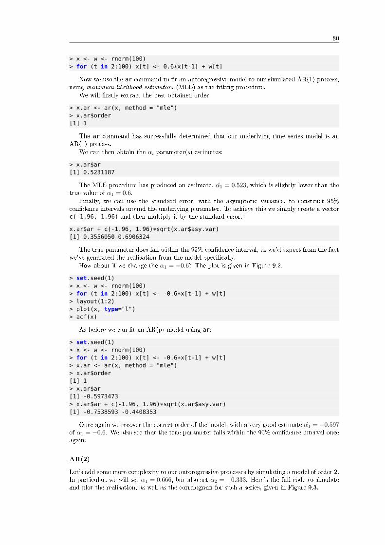
80

> x <- w <- rnorm(100)> for (t in 2:100) x[t] <- 0.6*x[t-1] + w[t]

Now we use the ar command to �t an autoregressive model to our simulated AR(1) process,using maximum likelihood estimation (MLE) as the �tting procedure.

We will �rstly extract the best obtained order:

> x.ar <- ar(x, method = "mle")> x.ar$order[1] 1

The ar command has successfully determined that our underlying time series model is anAR(1) process.

We can then obtain the αi parameter(s) estimates:

> x.ar$ar[1] 0.5231187

The MLE procedure has produced an estimate, α1 = 0.523, which is slightly lower than thetrue value of α1 = 0.6.

Finally, we can use the standard error, with the asymptotic variance, to construct 95%con�dence intervals around the underlying parameter. To achieve this we simply create a vectorc(-1.96, 1.96) and then multiply it by the standard error:

x.ar$ar + c(-1.96, 1.96)*sqrt(x.ar$asy.var)[1] 0.3556050 0.6906324

The true parameter does fall within the 95% con�dence interval, as we'd expect from the factwe've generated the realisation from the model speci�cally.

How about if we change the α1 = −0.6? The plot is given in Figure 9.2.

> set.seed(1)> x <- w <- rnorm(100)> for (t in 2:100) x[t] <- -0.6*x[t-1] + w[t]> layout(1:2)> plot(x, type="l")> acf(x)

As before we can �t an AR(p) model using ar:

> set.seed(1)> x <- w <- rnorm(100)> for (t in 2:100) x[t] <- -0.6*x[t-1] + w[t]> x.ar <- ar(x, method = "mle")> x.ar$order[1] 1> x.ar$ar[1] -0.5973473> x.ar$ar + c(-1.96, 1.96)*sqrt(x.ar$asy.var)[1] -0.7538593 -0.4408353

Once again we recover the correct order of the model, with a very good estimate α1 = −0.597of α1 = −0.6. We also see that the true parameter falls within the 95% con�dence interval onceagain.

AR(2)

Let's add some more complexity to our autoregressive processes by simulating a model of order 2.In particular, we will set α1 = 0.666, but also set α2 = −0.333. Here's the full code to simulateand plot the realisation, as well as the correlogram for such a series, given in Figure 9.3.

81

Figure 9.2: Realisation of AR(1) Model, with α1 = −0.6 and Associated Correlogram.

> set.seed(1)> x <- w <- rnorm(100)> for (t in 3:100) x[t] <- 0.666*x[t-1] - 0.333*x[t-2] + w[t]> layout(1:2)> plot(x, type="l")> acf(x)

As before we can see that the correlogram di�ers signi�cantly from that of white noise, aswe'd expect. There are statistically signi�cant peaks at k = 1, k = 3 and k = 4.

Once again, we're going to use the ar command to �t an AR(p) model to our underlyingAR(2) realisation. The procedure is similar as for the AR(1) �t:

> set.seed(1)> x <- w <- rnorm(100)> for (t in 3:100) x[t] <- 0.666*x[t-1] - 0.333*x[t-2] + w[t]> x.ar <- ar(x, method = "mle")Warning message:In arima0(x, order = c(i, 0L, 0L), include.mean = demean) :possible convergence problem: optim gave code = 1

> x.ar$order[1] 2> x.ar$ar[1] 0.6961005 -0.3946280

The correct order has been recovered and the parameter estimates α1 = 0.696 and α2 =−0.395 are not too far o� the true parameter values of α1 = 0.666 and α2 = −0.333.

Notice that we receive a convergence warning message. Notice also that R actually uses thearima0 function to calculate the AR model. As we'll learn in subsequent chapters, AR(p) modelsare simply ARIMA(p, 0, 0) models, and thus an AR model is a special case of ARIMA with noMoving Average (MA) or Integrated (I) component.

82

Figure 9.3: Realisation of AR(2) Model, with α1 = 0.666, α2 = −0.333 and Associated Correlo-gram.

We'll also be using the arima command to create con�dence intervals around multiple pa-rameters, which is why we've neglected to do it here.

Now that we've created some simulated data it is time to apply the AR(p) models to �nancialasset time series.

9.4.5 Financial Data

Amazon Inc.

Let's begin by obtaining the stock price for Amazon (AMZN) using quantmod as in the previouschapter:

> require(quantmod)> getSymbols("AMZN")> AMZN....2015-08-12 523.75 527.50 513.06 525.91 3962300 525.912015-08-13 527.37 534.66 525.49 529.66 2887800 529.662015-08-14 528.25 534.11 528.25 531.52 1983200 531.52

The �rst task is to always plot the price for a brief visual inspection. In this case we'll beusing the daily closing prices. The plot is given in Figure 9.4.

> plot(Cl(AMZN))

You'll notice that quantmod adds some formatting for us, namely the date, and a slightlyprettier chart than the usual R charts.

We are now going to take the logarithmic returns of AMZN and then the �rst-order di�er-ence of the series in order to convert the original price series from a non-stationary series to a(potentially) stationary one.

83

Figure 9.4: Daily Closing Price of AMZN.

This allows us to compare "apples to apples" between equities, indexes or any other asset,for use in later multivariate statistics, such as when calculating a covariance matrix.

Let's create a new series, amznrt, to hold our di�erenced log returns:

> amznrt = diff(log(Cl(AMZN)))

Once again, we can plot the series, as given in Figure 9.5.

> plot(amznrt)

At this stage we want to plot the correlogram. We're looking to see if the di�erenced serieslooks like white noise. If it does not then there is unexplained serial correlation, which might be"explained" by an autoregressive model. See Figure 9.6.

> acf(amznrt, na.action=na.omit)

We notice a statististically signi�cant peak at k = 2. Hence there is a reasonable possibilityof unexplained serial correlation. Be aware though, that this may be due to sampling bias. Assuch, we can try �tting an AR(p) model to the series and produce con�dence intervals for theparameters:

> amznrt.ar <- ar(amznrt, na.action=na.omit)> amznrt.ar$order[1] 2> amznrt.ar$ar[1] -0.02779869 -0.06873949> amznrt.ar$asy.var

[,1] [,2][1,] 4.59499e-04 1.19519e-05[2,] 1.19519e-05 4.59499e-04

Fitting the ar autoregressive model to the �rst order di�erenced series of log prices producesan AR(2) model, with α1 = −0.0278 and α2 = −0.0687. I've also output the aysmptotic variance

84

Figure 9.5: First Order Di�erenced Daily Logarithmic Returns of AMZN Closing Prices.

Figure 9.6: Correlogram of First Order Di�erenced Daily Logarithmic Returns of AMZN ClosingPrices.

so that we can calculate standard errors for the parameters and produce con�dence intervals.

85

We want to see whether zero is part of the 95% con�dence interval, as if it is, it reduces ourcon�dence that we have a true underlying AR(2) process for the AMZN series.

To calculate the con�dence intervals at the 95% level for each parameter, we use the followingcommands. We take the square root of the �rst element of the asymptotic variance matrix toproduce a standard error, then create con�dence intervals by multiplying it by -1.96 and 1.96respectively, for the 95% level:

> -0.0278 + c(-1.96, 1.96)*sqrt(4.59e-4)[1] -0.0697916 0.0141916> -0.0687 + c(-1.96, 1.96)*sqrt(4.59e-4)[1] -0.1106916 -0.0267084

Note that this becomes more straightforward when using the arima function, but we'll waituntil the next chapter before introducing it properly.

Thus we can see that for α1 zero is contained within the con�dence interval, while for α2 zerois not contained in the con�dence interval. Hence we should be very careful in thinking that wereally have an underlying generative AR(2) model for AMZN.

In particular we note that the autoregressive model does not take into account volatilityclustering, which leads to clustering of serial correlation in �nancial time series. When weconsider the ARCH and GARCH models in later chapters, we will account for this.

When we come to use the full arima function in the trading strategy section of the book, wewill make predictions of the daily log price series in order to allow us to create trading signals.

S&P500 US Equity Index

Along with individual stocks we can also consider the US Equity index, the S&P500. Let's applyall of the previous commands to this series and produce the plots as before:

> getSymbols("^GSPC")> GSPC....2015-08-12 2081.10 2089.06 2052.09 2086.05 4269130000 2086.052015-08-13 2086.19 2092.93 2078.26 2083.39 3221300000 2083.392015-08-14 2083.15 2092.45 2080.61 2091.54 2795590000 2091.54

We can plot the prices, as given in Figure 9.7.

> plot(Cl(GSPC))

As before, we'll create the �rst order di�erence of the log closing prices:

> gspcrt = diff(log(Cl(GSPC)))

Once again, we can plot the series, as given in Figure 9.8.

> plot(gspcrt)

It is clear from this chart that the volatility is not stationary in time. This is also re�ectedin the plot of the correlogram, given in Figure 9.9. There are many peaks, including k = 1 andk = 2, which are statistically signi�cant beyond a white noise model.

In addition, we see evidence of long-memory processes as there are some statistically signi�-cant peaks at k = 16, k = 18 and k = 21:

> acf(gspcrt, na.action=na.omit)

Ultimately we will need a more sophisticated model than an autoregressive model of order p.However, at this stage we can still try �tting such a model. Let's see what we get if we do so:

> gspcrt.ar <- ar(gspcrt, na.action=na.omit)> gspcrt.ar$order[1] 22> gspcrt.ar$ar

86

Figure 9.7: Daily Closing Price of S&500.

Figure 9.8: First Order Di�erenced Daily Logarithmic Returns of S&500 Closing Prices.

[1] -0.111821507 -0.060150504 0.018791594 -0.025619932 -0.046391435[6] 0.002266741 -0.030089046 0.030430265 -0.007623949 0.044260402

87

Figure 9.9: Correlogram of First Order Di�erenced Daily Logarithmic Returns of S&500 ClosingPrices.

[11] -0.018924358 0.032752930 -0.001074949 -0.042891664 -0.039712505[16] 0.052339497 0.016554471 -0.067496381 0.007070516 0.035721299[21] -0.035419555 0.031325869

Using ar produces an AR(22) model, i.e. a model with 22 non-zero parameters! What doesthis tell us? It is indicative that there is likely a lot more complexity in the serial correlationthan a simple linear model of past prices can really account for.

However, we already knew this because we can see that there is signi�cant serial correlationin the volatility. For instance, consider the highly volatile period around 2008.

This motivates the next set of models, namely the Moving Average MA(q) and the Autore-gressive Moving Average ARMA(p, q). We'll learn about both of these in the next couple ofsections of this chapter. As we repeatedly mention, these will ultimately lead us to the ARIMAand GARCH family of models, both of which will provide a much better �t to the serial corre-lation complexity of the S&P500.

This will allows us to improve our forecasts signi�cantly and ultimately produce more prof-itable strategies.

9.5 Moving Average (MA) Models of order q

In the previous section we considered the Autoregressive model of order p, also known as theAR(p) model. We introduced it as an extension of the random walk model in an attempt toexplain additional serial correlation in �nancial time series.

Ultimately we realised that it was not su�ciently �exible to truly capture all of the autocor-relation in the closing prices of Amazon Inc. (AMZN) and the S&P500 US Equity Index. Theprimary reason for this is that both of these assets are conditionally heteroskedastic, which meansthat they are non-stationary and have periods of "varying variance" or volatility clustering, whichis not taken into account by the AR(p) model.

88

In the next chapter we will consider the Autoregressive Integrated Moving Average (ARIMA)model, as well as the conditional heteroskedastic models of the ARCH and GARCH families.These models will provide us with our �rst realistic attempts at forecasting asset prices.

In this section, however, we are going to introduce theMoving Average of order q model,known as MA(q). This is a component of the more general ARMA model and as such we needto understand it before moving further.

9.5.1 Rationale

A Moving Average model is similar to an Autoregressive model, except that instead of being alinear combination of past time series values, it is a linear combination of the past white noiseterms.

Intuitively, this means that the MA model sees such random white noise "shocks" directly ateach current value of the model. This is in contrast to an AR(p) model, where the white noise"shocks" are only seen indirectly, via regression onto previous terms of the series.

A key di�erence is that the MA model will only ever see the last q shocks for any particularMA(q) model, whereas the AR(p) model will take all prior shocks into account, albeit in adecreasingly weak manner.

9.5.2 De�nition

Mathematically, the MA(q) is a linear regression model and is similarly structured to AR(p):

De�nition 9.5.1. Moving Average Model of order q. A time series model, {xt}, is a movingaverage model of order q, MA(q), if:

xt = wt + β1wt−1 + . . .+ βqwt−q (9.11)

Where {wt} is white noise with E(wt) = 0 and variance σ2.If we consider the Backward Shift Operator, B then we can rewrite the above as a function φ

of B:

xt = (1 + β1B + β2B2 + . . .+ βqB

q)wt = φq(B)wt (9.12)

We will make use of the φ function in subsequent chapters.

9.5.3 Second Order Properties

As with AR(p) the mean of a MA(q) process is zero. This is easy to see as the mean is simply asum of means of white noise terms, which are all themselves zero.

Mean: µx = E(xt) =

q∑i=0

E(wi) = 0 (9.13)

Var: σ2w(1 + β2

1 + . . .+ β2q ) (9.14)

ACF: ρk =

1 if k = 0

q−k∑i=0

βiβi+k/

q∑i=0

β2i if k = 1, . . . , q

0 if k > q

Where β0 = 1.We're now going to generate some simulated data and use it to create correlograms. This

will make the above formula for ρk somewhat more concrete.

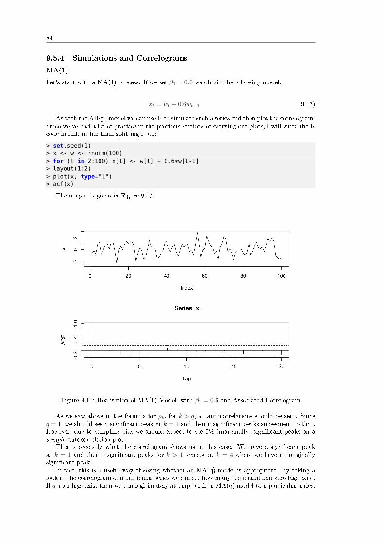
89

9.5.4 Simulations and Correlograms

MA(1)

Let's start with a MA(1) process. If we set β1 = 0.6 we obtain the following model:

xt = wt + 0.6wt−1 (9.15)

As with the AR(p) model we can use R to simulate such a series and then plot the correlogram.Since we've had a lot of practice in the previous sections of carrying out plots, I will write the Rcode in full, rather than splitting it up:

> set.seed(1)> x <- w <- rnorm(100)> for (t in 2:100) x[t] <- w[t] + 0.6*w[t-1]> layout(1:2)> plot(x, type="l")> acf(x)

The output is given in Figure 9.10.

Figure 9.10: Realisation of MA(1) Model, with β1 = 0.6 and Associated Correlogram

As we saw above in the formula for ρk, for k > q, all autocorrelations should be zero. Sinceq = 1, we should see a signi�cant peak at k = 1 and then insigni�cant peaks subsequent to that.However, due to sampling bias we should expect to see 5% (marginally) signi�cant peaks on asample autocorrelation plot.

This is precisely what the correlogram shows us in this case. We have a signi�cant peakat k = 1 and then insigni�cant peaks for k > 1, except at k = 4 where we have a marginallysigni�cant peak.

In fact, this is a useful way of seeing whether an MA(q) model is appropriate. By taking alook at the correlogram of a particular series we can see how many sequential non-zero lags exist.If q such lags exist then we can legitimately attempt to �t a MA(q) model to a particular series.

90

Since we have evidence from our simulated data of a MA(1) process, we're now going totry and �t a MA(1) model to our simulated data. Unfortunately, there isn't an equivalent macommand to the autoregressive model ar command in R.

Instead, we must use the more general arima command and set the autoregressive and inte-grated components to zero. We do this by creating a 3-vector and setting the �rst two components(the autogressive and integrated parameters, respectively) to zero:

> x.ma <- arima(x, order=c(0, 0, 1))> x.ma

Call:arima(x = x, order = c(0, 0, 1))

Coefficients:ma1 intercept

0.6023 0.1681s.e. 0.0827 0.1424

sigma^2 estimated as 0.7958: log likelihood = -130.7, aic = 267.39

We receive some useful output from the arima command. Firstly, we can see that theparameter has been estimated as β1 = 0.602, which is very close to the true value of β1 =0.6. Secondly, the standard errors are already calculated for us, making it straightforward tocalculate con�dence intervals. Thirdly, we receive an estimated variance, log-likelihood andAkaike Information Criterion (necessary for model comparison).

The major di�erence between arima and ar is that arima estimates an intercept term becauseit does not subtract the mean value of the series. Hence we need to be careful when carrying outpredictions using the arima command. We'll return to this point later.

As a quick check we're going to calculate con�dence intervals for β1:

> 0.6023 + c(-1.96, 1.96)*0.0827[1] 0.440208 0.764392

We can see that the 95% con�dence interval contains the true parameter value of β1 = 0.6and so we can judge the model a good �t. Obviously this should be expected since we simulatedthe data in the �rst place!

How do things change if we modify the sign of β1 to -0.6? Let's perform the same analysis:

> set.seed(1)> x <- w <- rnorm(100)> for (t in 2:100) x[t] <- w[t] - 0.6*w[t-1]> layout(1:2)> plot(x, type="l")> acf(x)

The output is given in Figure 9.11.We can see that at k = 1 we have a signi�cant peak in the correlogram, except that it

shows negative correlation, as we'd expect from a MA(1) model with negative �rst coe�cient.Once again all peaks beyond k = 1 are insigni�cant. Let's �t a MA(1) model and estimate theparameter:

> x.ma <- arima(x, order=c(0, 0, 1))> x.ma

Call:arima(x = x, order = c(0, 0, 1))

Coefficients:ma1 intercept

-0.7298 0.0486

91

Figure 9.11: Realisation of MA(1) Model, with β1 = −0.6 and Associated Correlogram

s.e. 0.1008 0.0246

sigma^2 estimated as 0.7841: log likelihood = -130.11, aic = 266.23

β1 = −0.730, which is a small underestimate of β1 = −0.6. Finally, let's calculate thecon�dence interval:

> -0.730 + c(-1.96, 1.96)*0.1008[1] -0.927568 -0.532432

We can see that the true parameter value of β1 = −0.6 is contained within the 95% con�denceinterval, providing us with evidence of a good model �t.

MA(3)

Let's run through the same procedure for a MA(3) process. This time we should expect signi�cantpeaks at k ∈ {1, 2, 3}, and insigni�cant peaks for k > 3.

We are going to use the following coe�cients: β1 = 0.6, β2 = 0.4 and β3 = 0.3. Let's simulatea MA(3) process from this model. I've increased the number of random samples to 1000 in thissimulation, which makes it easier to see the true autocorrelation structure, at the expense ofmaking the original series harder to interpret:

> set.seed(3)> x <- w <- rnorm(1000)> for (t in 4:1000) x[t] <- w[t] + 0.6*w[t-1] + 0.4*w[t-2] + 0.3*w[t-3]> layout(1:2)> plot(x, type="l")> acf(x)

The output is given in Figure 9.12.

92

Figure 9.12: Realisation of MA(3) Model and Associated Correlogram

As expected the �rst three peaks are signi�cant. However, so is the fourth. But we canlegitimately suggest that this may be due to sampling bias as we expect to see 5% of the peaksbeing signi�cant beyond k = q.

Let's now �t a MA(3) model to the data to try and estimate parameters:

> x.ma <- arima(x, order=c(0, 0, 3))> x.ma

Call:arima(x = x, order = c(0, 0, 3))

Coefficients:ma1 ma2 ma3 intercept

0.5439 0.3450 0.2975 -0.0948s.e. 0.0309 0.0349 0.0311 0.0704

sigma^2 estimated as 1.039: log likelihood = -1438.47, aic = 2886.95

The estimates β1 = 0.544, β2 = 0.345 and β3 = 0.298 are close to the true values of β1 = 0.6,β2 = 0.4 and β3 = 0.3, respectively. We can also produce con�dence intervals using the respectivestandard errors:

> 0.544 + c(-1.96, 1.96)*0.0309[1] 0.483436 0.604564> 0.345 + c(-1.96, 1.96)*0.0349[1] 0.276596 0.413404> 0.298 + c(-1.96, 1.96)*0.0311[1] 0.237044 0.358956

In each case the 95% con�dence intervals do contain the true parameter value and we canconclude that we have a good �t with our MA(3) model, as should be expected.

93

9.5.5 Financial Data

In the previous section we considered Amazon Inc. (AMZN) and the S&P500 US Equity Index.We �tted the AR(p) model to both and found that the model was unable to e�ectively capturethe complexity of the serial correlation, especially in the case of the S&P500, where conditionalheteroskedastic and long-memory e�ects seem to be present.

Amazon Inc. (AMZN)

Let's begin by trying to �t a selection of MA(q) models to AMZN, namely with q ∈ {1, 2, 3}. Asin the previous section, we'll use quantmod to download the daily prices for AMZN and thenconvert them into a log returns stream of closing prices:

> require(quantmod)> getSymbols("AMZN")> amznrt = diff(log(Cl(AMZN)))

Now that we have the log returns stream we can use the arima command to �t MA(1), MA(2)and MA(3) models and then estimate the parameters of each. For MA(1) we have:

> amznrt.ma <- arima(amznrt, order=c(0, 0, 1))> amznrt.ma

Call:arima(x = amznrt, order = c(0, 0, 1))

Coefficients:ma1 intercept

-0.030 0.0012s.e. 0.023 0.0006

sigma^2 estimated as 0.0007044: log likelihood = 4796.01, aic = -9586.02

We can plot the residuals of the daily log returns and the �tted model, given in Figure 9.13.

> acf(amznrt.ma$res[-1])

Notice that we have a few signi�cant peaks at lags k = 2, k = 11, k = 16 and k = 18,indicating that the MA(1) model is unlikely to be a good �t for the behaviour of the AMZN logreturns, since this does not look like a realisation of white noise.

Let's try a MA(2) model:

> amznrt.ma <- arima(amznrt, order=c(0, 0, 2))> amznrt.ma

Call:arima(x = amznrt, order = c(0, 0, 2))

Coefficients:ma1 ma2 intercept

-0.0254 -0.0689 0.0012s.e. 0.0215 0.0217 0.0005

sigma^2 estimated as 0.0007011: log likelihood = 4801.02, aic = -9594.05

Both of the estimates for the β coe�cients are negative. Let's plot the residuals once again,given in Figure 9.14.

> acf(amznrt.ma$res[-1])

We can see that there is almost zero autocorrelation in the �rst few lags. However, we have�ve marginally signi�cant peaks at lags k = 12, k = 16, k = 19, k = 25 and k = 27. This is

94

Figure 9.13: Residuals of MA(1) Model Fitted to AMZN Daily Log Prices

Figure 9.14: Residuals of MA(2) Model Fitted to AMZN Daily Log Prices

suggestive that the MA(2) model is capturing a lot of the autocorrelation, but not all of thelong-memory e�ects. How about a MA(3) model?

95

> amznrt.ma <- arima(amznrt, order=c(0, 0, 3))> amznrt.ma

Call:arima(x = amznrt, order = c(0, 0, 3))

Coefficients:ma1 ma2 ma3 intercept

-0.0262 -0.0690 0.0177 0.0012s.e. 0.0214 0.0217 0.0212 0.0005

sigma^2 estimated as 0.0007009: log likelihood = 4801.37, aic = -9592.75

Once again, we can plot the residuals, as given in Figure 9.15.

> acf(amznrt.ma$res[-1])

Figure 9.15: Residuals of MA(3) Model Fitted to AMZN Daily Log Prices

The MA(3) residuals plot looks almost identical to that of the MA(2) model. This is notsurprising, as we're adding a new parameter to a model that has seemingly explained away muchof the correlations at shorter lags, but that won't have much of an e�ect on the longer term lags.

All of this evidence is suggestive of the fact that an MA(q) model is unlikely to be useful inexplaining all of the serial correlation in isolation, at least for AMZN.

S&P500

If you recall in the previous section we saw that the �rst order di�erenced daily log returnsstructure of the S&P500 possessed many signi�cant peaks at various lags, both short and long.This provided evidence of both conditional heteroskedasticity (i.e. volatility clustering) and long-memory e�ects. It lead us to conclude that the AR(p) model was insu�cient to capture all ofthe autocorrelation present.

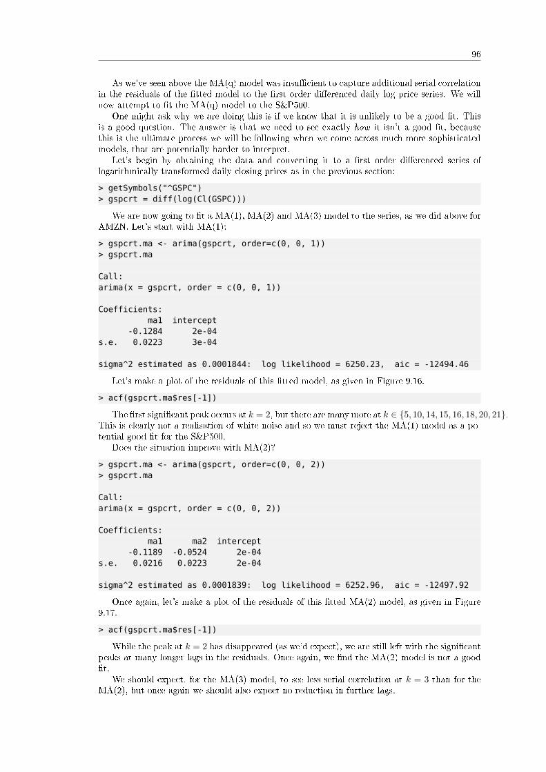
96

As we've seen above the MA(q) model was insu�cient to capture additional serial correlationin the residuals of the �tted model to the �rst order di�erenced daily log price series. We willnow attempt to �t the MA(q) model to the S&P500.

One might ask why we are doing this is if we know that it is unlikely to be a good �t. Thisis a good question. The answer is that we need to see exactly how it isn't a good �t, becausethis is the ultimate process we will be following when we come across much more sophisticatedmodels, that are potentially harder to interpret.

Let's begin by obtaining the data and converting it to a �rst order di�erenced series oflogarithmically transformed daily closing prices as in the previous section:

> getSymbols("^GSPC")> gspcrt = diff(log(Cl(GSPC)))

We are now going to �t a MA(1), MA(2) and MA(3) model to the series, as we did above forAMZN. Let's start with MA(1):

> gspcrt.ma <- arima(gspcrt, order=c(0, 0, 1))> gspcrt.ma

Call:arima(x = gspcrt, order = c(0, 0, 1))

Coefficients:ma1 intercept

-0.1284 2e-04s.e. 0.0223 3e-04

sigma^2 estimated as 0.0001844: log likelihood = 6250.23, aic = -12494.46

Let's make a plot of the residuals of this �tted model, as given in Figure 9.16.

> acf(gspcrt.ma$res[-1])

The �rst signi�cant peak occurs at k = 2, but there are many more at k ∈ {5, 10, 14, 15, 16, 18, 20, 21}.This is clearly not a realisation of white noise and so we must reject the MA(1) model as a po-tential good �t for the S&P500.

Does the situation improve with MA(2)?

> gspcrt.ma <- arima(gspcrt, order=c(0, 0, 2))> gspcrt.ma

Call:arima(x = gspcrt, order = c(0, 0, 2))

Coefficients:ma1 ma2 intercept

-0.1189 -0.0524 2e-04s.e. 0.0216 0.0223 2e-04

sigma^2 estimated as 0.0001839: log likelihood = 6252.96, aic = -12497.92

Once again, let's make a plot of the residuals of this �tted MA(2) model, as given in Figure9.17.

> acf(gspcrt.ma$res[-1])

While the peak at k = 2 has disappeared (as we'd expect), we are still left with the signi�cantpeaks at many longer lags in the residuals. Once again, we �nd the MA(2) model is not a good�t.

We should expect, for the MA(3) model, to see less serial correlation at k = 3 than for theMA(2), but once again we should also expect no reduction in further lags.

97

Figure 9.16: Residuals of MA(1) Model Fitted to S&P500 Daily Log Prices

Figure 9.17: Residuals of MA(2) Model Fitted to S&P500 Daily Log Prices

> gspcrt.ma <- arima(gspcrt, order=c(0, 0, 3))> gspcrt.ma

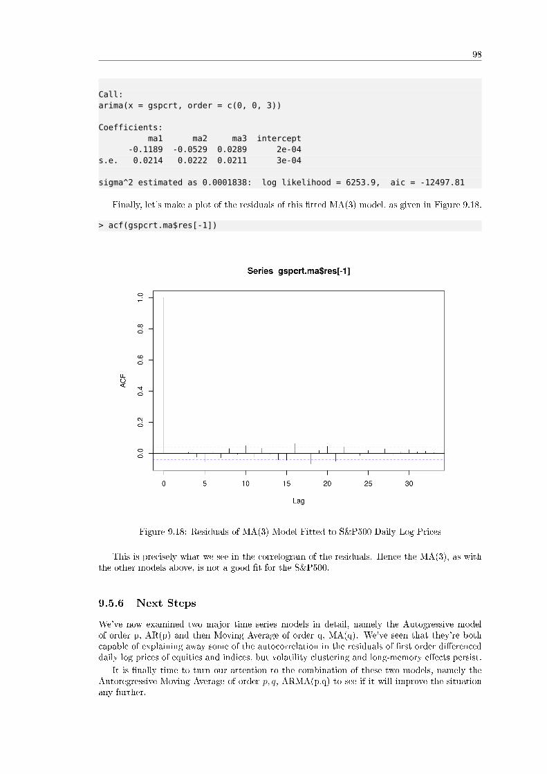
98

Call:arima(x = gspcrt, order = c(0, 0, 3))

Coefficients:ma1 ma2 ma3 intercept

-0.1189 -0.0529 0.0289 2e-04s.e. 0.0214 0.0222 0.0211 3e-04

sigma^2 estimated as 0.0001838: log likelihood = 6253.9, aic = -12497.81

Finally, let's make a plot of the residuals of this �tted MA(3) model, as given in Figure 9.18.

> acf(gspcrt.ma$res[-1])

Figure 9.18: Residuals of MA(3) Model Fitted to S&P500 Daily Log Prices

This is precisely what we see in the correlogram of the residuals. Hence the MA(3), as withthe other models above, is not a good �t for the S&P500.

9.5.6 Next Steps

We've now examined two major time series models in detail, namely the Autogressive modelof order p, AR(p) and then Moving Average of order q, MA(q). We've seen that they're bothcapable of explaining away some of the autocorrelation in the residuals of �rst order di�erenceddaily log prices of equities and indices, but volatility clustering and long-memory e�ects persist.

It is �nally time to turn our attention to the combination of these two models, namely theAutoregressive Moving Average of order p, q, ARMA(p,q) to see if it will improve the situationany further.

99

9.6 Autogressive Moving Average (ARMA) Models of orderp, q

We've introduced Autoregressive models and Moving Average models in the two previous sections.Now it is time to combine them to produce a more sophisticated model.

Ultimately this will lead us to the ARIMA and GARCH models that will allow us to predictasset returns and forecast volatility. These models will form the basis for trading signals andrisk management techniques.

If you've read the previous sections in this chapter you will have seen that we tend to followa pattern for our analysis of a time series model. I'll repeat it brie�y here:

� Rationale - Why are we interested in this particular model?

� De�nition - A mathematical de�nition to reduce ambiguity.

� Correlogram - Plotting a sample correlogram to visualise a models behaviour.

� Simulation and Fitting - Fitting the model to simulations, in order to ensure we'veunderstood the model correctly.

� Real Financial Data - Apply the model to real historical asset prices.

However, before delving into the ARMA model we need to discuss the Bayesian InformationCriterion and the Ljung-Box test, two essential tools for helping us to choose the correct modeland ensuring that any chosen model is a good �t.

9.6.1 Bayesian Information Criterion

In the previous section we looked at the Akaike Information Criterion (AIC) as a means of helpingus choose between separate "best" time series models.

A closely related tool is the Bayesian Information Criterion (BIC). Essentially it hassimilar behaviour to the AIC in that it penalises models for having too many parameters. Thismay lead to over�tting. The di�erence between the BIC and AIC is that the BIC is more stringentwith its penalisation of additional parameters.

De�nition 9.6.1. Bayesian Information Criterion. If we take the likelihood function for astatistical model, which has k parameters, and L maximises the likelihood, then the BayesianInformation Criterion is given by:

BIC = −2log(L) + klog(n) (9.16)

Where n is the number of data points in the time series.

We will be using the AIC and BIC below when choosing appropriate ARMA(p,q) models.

9.6.2 Ljung-Box Test

The Ljung-Box test is a classical (in a statistical sense) hypothesis test that is designed to testwhether a set of autocorrelations of a �tted time series model di�er signi�cantly from zero. Thetest does not test each individual lag for randomness, but rather tests the randomness over agroup of lags. Formally:

De�nition 9.6.2. Ljung-Box Test. We de�ne the null hypothesis H0 as: The time series dataat each lag are independent and identically distributed (i.i.d.), that is, the correlations betweenthe population series values are zero.

We de�ne the alternate hypothesis Ha as: The time series data are not i.i.d. and possessserial correlation.

We calculate the following test statistic, Q:

100

Q = n(n+ 2)

h∑k=1

ρ2k

n− k(9.17)

Where n is the length of the time series sample, ρk is the sample autocorrelation at lag k andh is the number of lags under the test.

The decision rule as to whether to reject the null hypothesisH0 is to check whether Q > χ2α,h,

for a chi-squared distribution with h degrees of freedom at the 100(1− α)th percentile.

While the details of the test may seem slightly complex, we can in fact use R to calculate thetest for us, simplifying the procedure somewhat.

Now that we've discussed the BIC and the Ljung-Box test, we're ready to discuss our �rstmixed model, namely the Autoregressive Moving Average of order p, q, or ARMA(p,q).

9.6.3 Rationale

To date we have considered autoregressive processes and moving average processes.The former model considers its own past behaviour as inputs for the model and as such

attempts to capture market participant e�ects, such as momentum and mean-reversion in stocktrading. The latter model is used to characterise "shock" information to a series, such as asurprise earnings announcement or other unexpected event. A good example of "shock" newswould be the BP Deepwater Horizon oil spill.

Hence, an ARMA model attempts to capture both of these aspects when modelling �nancialtime series. Note however that it does not take into account volatility clustering, a key empiricalphenomena of many �nancial time series. It is not a conditional heteroskedastic model. For thatwe will need to wait for the ARCH and GARCH models.

9.6.4 De�nition

The ARMA(p,q) model is a linear combination of two linear models and thus is itself still linear:

De�nition 9.6.3. Autoregressive Moving Average Model of order p, q. A time series model,{xt}, is an autoregressive moving average model of order p, q, ARMA(p,q), if:

xt = α1xt−1 + α2xt−2 + . . .+ wt + β1wt−1 + β2wt−2 . . .+ βqwt−q (9.18)

Where {wt} is white noise with E(wt) = 0 and variance σ2.If we consider the Backward Shift Operator, B then we can rewrite the above as a function θ

and φ of B:

θp(B)xt = φq(B)wt (9.19)

We can straightforwardly see that by setting p 6= 0 and q = 0 we recover the AR(p) model.Similarly if we set p = 0 and q 6= 0 we recover the MA(q) model.

One of the key features of the ARMA model is that it is parsimonious and redundant in itsparameters. That is, an ARMA model will often require fewer parameters than an AR(p) orMA(q) model alone. In addition if we rewrite the equation in terms of the BSO, then the θ andφ polynomials can sometimes share a common factor, thus leading to a simpler model.

9.6.5 Simulations and Correlograms

As with the autoregressive and moving average models we will now simulate various ARMAseries and then attempt to �t ARMA models to these realisations. We carry this out because wewant to ensure that we understand the �tting procedure, including how to calculate con�denceintervals for the models, as well as ensure that the procedure does actually recover reasonableestimates for the original ARMA parameters.

101

In the previous sections we manually constructed the AR and MA series by drawing Nsamples from a normal distribution and then crafting the speci�c time series model using lags ofthese samples.

However, there is a more straightforward way to simulate AR, MA, ARMA and even ARIMAdata, simply by using the arima.sim method in R.

Let's start with the simplest possible non-trivial ARMA model, namely the ARMA(1,1)model. That is, an autoregressive model of order one combined with a moving average model oforder one. Such a model has only two coe�cients, α and β, which represent the �rst lags of thetime series itself and the "shock" white noise terms. Such a model is given by:

xt = αxt−1 + wt + βwt−1 (9.20)

We need to specify the coe�cients prior to simulation. Let's take α = 0.5 and β = −0.5:

> set.seed(1)> x <- arima.sim(n=1000, model=list(ar=0.5, ma=-0.5))> plot(x)

The output is given in Figure 9.19.

Figure 9.19: Realisation of an ARMA(1,1) Model, with α = 0.5 and β = −0.5

Let's also plot the correlogram, as given in Figure 9.20.

> acf(x)

We can see that there is no signi�cant autocorrelation, which is to be expected from anARMA(1,1) model.

Finally, let's try and determine the coe�cients and their standard errors using the arimafunction:

> arima(x, order=c(1, 0, 1))

Call:

102

Figure 9.20: Correlogram of an ARMA(1,1) Model, with α = 0.5 and β = −0.5

arima(x = x, order = c(1, 0, 1))

Coefficients:ar1 ma1 intercept

-0.3957 0.4503 0.0538s.e. 0.3727 0.3617 0.0337

sigma^2 estimated as 1.053: log likelihood = -1444.79, aic = 2897.58

We can calculate the con�dence intervals for each parameter using the standard errors:

> -0.396 + c(-1.96, 1.96)*0.373[1] -1.12708 0.33508> 0.450 + c(-1.96, 1.96)*0.362[1] -0.25952 1.15952

The con�dence intervals do contain the true parameter values for both cases, however weshould note that the 95% con�dence intervals are very wide (a consequence of the reasonablylarge standard errors).

Let's now try an ARMA(2,2) model. That is, an AR(2) model combined with a MA(2)model. We need to specify four parameters for this model: α1, α2, β1 and β2. Let's takeα1 = 0.5, α2 = −0.25 β1 = 0.5 and β2 = −0.3:

> set.seed(1)> x <- arima.sim(n=1000, model=list(ar=c(0.5, -0.25), ma=c(0.5, -0.3)))> plot(x)

The output of our ARMA(2,2) model is given in Figure 9.21.And the corresponding autocorelation, as given in Figure 9.22.

> acf(x)

We can now try �tting an ARMA(2,2) model to the data:

103

Figure 9.21: Realisation of an ARMA(2,2) Model, with α1 = 0.5, α2 = −0.25, β1 = 0.5 andβ2 = −0.3

Figure 9.22: Correlogram of an ARMA(2,2) Model, with α1 = 0.5, α2 = −0.25, β1 = 0.5 andβ2 = −0.3

104

> arima(x, order=c(2, 0, 2))

Call:arima(x = x, order = c(2, 0, 2))

Coefficients:ar1 ar2 ma1 ma2 intercept

0.6529 -0.2291 0.3191 -0.5522 -0.0290s.e. 0.0802 0.0346 0.0792 0.0771 0.0434

sigma^2 estimated as 1.06: log likelihood = -1449.16, aic = 2910.32

We can also calculate the con�dence intervals for each parameter:

> 0.653 + c(-1.96, 1.96)*0.0802[1] 0.495808 0.810192> -0.229 + c(-1.96, 1.96)*0.0346[1] -0.296816 -0.161184> 0.319 + c(-1.96, 1.96)*0.0792[1] 0.163768 0.474232> -0.552 + c(-1.96, 1.96)*0.0771[1] -0.703116 -0.400884

Notice that the con�dence intervals for the coe�cients for the moving average component(β1 and β2) do not actually contain the original parameter value. This outlines the danger ofattempting to �t models to data, even when we know the true parameter values!

However, for trading purposes we just need to have a predictive power that exceeds chanceand produces enough pro�t above transaction costs, in order to be pro�table in the long run.

Now that we've seen some examples of simulated ARMA models we need a mechanism forchoosing the values of p and q when �tting to the models to real �nancial data.

9.6.6 Choosing the Best ARMA(p,q) Model

In order to determine which order p, q of the ARMA model is appropriate for a series, we needto use the AIC (or BIC) across a subset of values for p, q, and then apply the Ljung-Box test todetermine if a good �t has been achieved, for particular values of p, q.

To show this method we are going to �rstly simulate a particular ARMA(p,q) process. Wewill then loop over all pairwise values of p ∈ {0, 1, 2, 3, 4} and q ∈ {0, 1, 2, 3, 4} and calculatethe AIC. We will select the model with the lowest AIC and then run a Ljung-Box test on theresiduals to determine if we have achieved a good �t.

Let's begin by simulating an ARMA(3,2) series:

> set.seed(3)> x <- arima.sim(n=1000, model=list(ar=c(0.5, -0.25, 0.4), ma=c(0.5, -0.3)))

We will now create an object final to store the best model �t and lowest AIC value. We loopover the various p, q combinations and use the current object to store the �t of an ARMA(i,j)model, for the looping variables i and j.

If the current AIC is less than any previously calculated AIC we set the �nal AIC to thiscurrent value and select that order. Upon termination of the loop we have the order of theARMA model stored in final.order and the ARIMA(p,d,q) �t itself (with the "Integrated" dcomponent set to 0) stored as final.arma:

> final.aic <- Inf> final.order <- c(0,0,0)> for (i in 0:4) for (j in 0:4) {> current.aic <- AIC(arima(x, order=c(i, 0, j)))> if (current.aic < final.aic) {> final.aic <- current.aic

105

> final.order <- c(i, 0, j)> final.arma <- arima(x, order=final.order)> }> }

Let's output the AIC, order and ARIMA coe�cients:

> final.aic[1] 2863.365

> final.order[1] 3 0 2

> final.arma

Call:arima(x = x, order = final.order)

Coefficients:ar1 ar2 ar3 ma1 ma2 intercept

0.4470 -0.2822 0.4079 0.5519 -0.2367 0.0274s.e. 0.0867 0.0345 0.0309 0.0954 0.0905 0.0975

sigma^2 estimated as 1.009: log likelihood = -1424.68, aic = 2863.36

We can see that the original order of the simulated ARMA model was recovered, namely withp = 3 and q = 2. We can plot the corelogram of the residuals of the model to see if they looklike a realisation of discrete white noise (DWN), as given in Figure 9.23.

> acf(resid(final.arma))

Figure 9.23: Correlogram of the residuals of the best �tting ARMA(p,q) Model, p = 3 and q = 2

106

The corelogram does indeed look like a realisation of DWN. Finally, we perform the Ljung-Boxtest for 20 lags to con�rm this:

> Box.test(resid(final.arma), lag=20, type="Ljung-Box")

Box-Ljung test

data: resid(final.arma)X-squared = 13.1927, df = 20, p-value = 0.869

Notice that the p-value is greater than 0.05, which states that the residuals are independentat the 95% level and thus an ARMA(3,2) model provides a good model �t.

Clearly this should be the case since we've simulated the data ourselves! However, this isprecisely the procedure we will use when we come to �t ARMA(p,q) models to the S&P500 indexin the following section.

9.6.7 Financial Data

Now that we've outlined the procedure for choosing the optimal time series model for a simulatedseries, it is rather straightforward to apply it to �nancial data. For this example we are going toonce again choose the S&P500 US Equity Index.

Let's download the daily closing prices using quantmod and then create the log returnsstream:

> require(quantmod)> getSymbols("^GSPC")> sp = diff(log(Cl(GSPC)))

Let's perform the same �tting procedure as for the simulated ARMA(3,2) series above on thelog returns series of the S&P500 using the AIC:

> spfinal.aic <- Inf> spfinal.order <- c(0,0,0)> for (i in 0:4) for (j in 0:4) {> spcurrent.aic <- AIC(arima(sp, order=c(i, 0, j)))> if (spcurrent.aic < spfinal.aic) {> spfinal.aic <- spcurrent.aic> spfinal.order <- c(i, 0, j)> spfinal.arma <- arima(sp, order=spfinal.order)> }> }

The best �tting model has order ARMA(3,3):

> spfinal.order[1] 3 0 3

Let's plot the residuals of the �tted model to the S&P500 log daily returns stream, as givenin Figure 9.24:

> acf(resid(spfinal.arma), na.action=na.omit)

Notice that there are some signi�cant peaks, especially at higher lags. This is indicative of apoor �t. Let's perform a Ljung-Box test to see if we have statistical evidence for this:

> Box.test(resid(spfinal.arma), lag=20, type="Ljung-Box")

Box-Ljung test

data: resid(spfinal.arma)X-squared = 37.1912, df = 20, p-value = 0.0111

107

Figure 9.24: Correlogram of the residuals of the best �tting ARMA(p,q) Model, p = 3 and q = 3,to the S&P500 daily log returns stream

As we suspected, the p-value is less that 0.05 and as such we cannot say that the residuals area realisation of discrete white noise. Hence there is additional autocorrelation in the residualsthat is not explained by the �tted ARMA(3,3) model.

9.7 Next Steps

As we've discussed all along in this part of the book we have seen evidence of conditional het-eroskedasticity (volatility clustering) in the S&P500 series, especially in the periods around 2007-2008. When we use a GARCH model in the next chapter we will see how to eliminate theseautocorrelations.

In practice, ARMA models are never generally good �ts for log equities returns. We needto take into account the conditional heteroskedasticity and use a combination of ARIMA andGARCH. The next chapter will consider ARIMA and show how the "Integrated" componentdi�ers from the ARMA model we have been considering in this chapter.

108

Chapter 10

Autoregressive Integrated MovingAverage and ConditionalHeteroskedastic Models

In the previous chapter we went into signi�cant detail about the AR(p), MA(q) and ARMA(p,q)linear time series models. We used these models to generate simulated data sets, �tted modelsto recover parameters and then applied these models to �nancial equities data.

In this chapter we are going to discuss an extension of the ARMA model, namely the Au-toregressive Integrated Moving Average model, or ARIMA(p,d,q) model as well as models thatincorporate conditional heteroskedasticity, such as ARCH and GARCH.

We will see that it is necessary to consider the ARIMA model when we have non-stationaryseries. Such series occur in the presence of stochastic trends.

10.1 Quick Recap

We have steadily built up our understanding of time series with concepts such as serial corre-lation, stationarity, linearity, residuals, correlograms, simulating, �tting, seasonality, conditionalheteroscedasticity and hypothesis testing.

As of yet we have not carried out any prediction or forecasting from our models and so havenot had any mechanism for producing a trading system or equity curve.

Once we have studied ARIMA we will be in a position to build a basic long-term tradingstrategy based on prediction of stock market index returns.

Despite the fact that I have gone into a lot of detail about models which we know willultimately not have great performance (AR, MA, ARMA), we are now well-versed in the processof time series modeling.

This means that when we come to study more recent models (and even those currently inthe research literature), we will have a signi�cant knowledge base on which to draw, in order toe�ectively evaluate these models, instead of treating them as a "turn key" prescription or "blackbox".

More importantly, it will provide us with the con�dence to extend and modify them on ourown and understand what we are doing when we do it!

I'd like to thank you for being patient so far, as it might seem that these chapters on timeseries analysis theory are far away from the "real action" of actual trading. However, truequantitative trading research is careful, measured and takes signi�cant time to get right. Thereis no quick �x or "get rich scheme" in quant trading.

We're very nearly ready to consider our �rst trading model, which will be a mixture of ARIMAand GARCH, so it is imperative that we spend some time understanding the ARIMA model well!

Once we have built our �rst trading model, we are going to consider more advanced modelsin subsequent chapters including long-memory processes, state-space models (i.e. the Kalman

109

110

Filter) and Vector Autoregressive (VAR) models, which will lead us to other, more sophisticated,trading strategies.

10.2 Autoregressive Integrated Moving Average (ARIMA)Models of order p, d, q

10.2.1 Rationale

ARIMA models are used because they can reduce a non-stationary series to a stationary seriesusing a sequence of di�erencing steps.

We can recall from the previous chapter on white noise and random walks that if we applythe di�erence operator to a random walk series {xt} (a non-stationary series) we are left withwhite noise {wt} (a stationary series):

∇xt = xt − xt−1 = wt (10.1)

ARIMA essentially performs this function but does so repeatedly d times in order to reducea non-stationary series to a stationary one. In order to handle other forms of non-stationaritybeyond stochastic trends additional models can be used.

Seasonality e�ects such as those that occur in commodity prices can be tackled with theSeasonal ARIMA model (SARIMA), however we won't be discussing SARIMA much in thisbook. Conditional heteroskedastic e�ects, such as volatility clustering in equities indexes, canbe tackled with ARCH and GARCH, which we discuss later in this chapter.

In this chapter we will �rst be considering non-stationary series with stochastic trends and�t ARIMA models to these series. We will also �nally produce forecasts for our �nancial series.

10.2.2 De�nitions

Prior to de�ning ARIMA processes we need to discuss the concept of an integrated series:

De�nition 10.2.1. Integrated Series of order d. A time series {xt} is integrated of order d, I(d),if:

∇dxt = wt (10.2)

That is, if we di�erence the series d times we receive a discrete white noise series.Alternatively, using the Backward Shift Operator B an equivalent condition is:

(1−Bd)xt = wt (10.3)

Now that we have de�ned an integrated series we can de�ne the ARIMA process itself:

De�nition 10.2.2. Autoregressive Integrated Moving Average Model of order p, d, q. A timeseries {xt} is an autoregressive integrated moving average model of order p, d, q,ARIMA(p,d,q),if ∇dxt is an autoregressive moving average model of order p,q, ARMA(p,q).

That is, if the series {xt} is di�erenced d times, and it then follows an ARMA(p,q) process,then it is an ARIMA(p,d,q) series.

If we use the polynomial notation from the previous chapter on ARMA then an ARIMA(p,d,q)process can be written in terms of the Backward Shift Operator, B:

θp(B)(1−B)dxt = φq(B)wt (10.4)

Where wt is a discrete white noise series.

111

There are some points to note about these de�nitions.Since the random walk is given by xt = xt−1 + wt it can be seen that I(1) is another

representation, since ∇1xt = wt.If we suspect a non-linear trend then we might be able to use repeated di�erencing (i.e. d > 1)

to reduce a series to stationary white noise. In R we can use the diff command with additionalparameters, e.g. diff(x, d=3) to carry out repeated di�erences.

10.2.3 Simulation, Correlogram and Model Fitting

Since we have already made use of the arima.sim command to simulate an ARMA(p,q) process,the following procedure will be similar to that carried out in the previous chapter.

The major di�erence is that we will now set d = 1, that is, we will produce a non-stationarytime series with a stochastic trending component.

As before we will �t an ARIMA model to our simulated data, attempt to recover the param-eters, create con�dence intervals for these parameters, produce a correlogram of the residuals ofthe �tted model and �nally carry out a Ljung-Box test to establish whether we have a good �t.

We are going to simulate an ARIMA(1,1,1) model, with the autoregressive coe�cient α = 0.6and the moving average coe�cient β = −0.5. Here is the R code to simulate and plot such aseries, see Figure 10.1.

> set.seed(2)> x <- arima.sim(list(order = c(1,1,1), ar = 0.6, ma=-0.5), n = 1000)> plot(x)

Figure 10.1: Plot of simulated ARIMA(1,1,1) model with α = 0.6 and β = −0.5

Now that we have our simulated series we are going to try and �t an ARIMA(1,1,1) modelto it. Since we know the order we will simply specify it in the �t:

> x.arima <- arima(x, order=c(1, 1, 1))

Call:

112

arima(x = x, order = c(1, 1, 1))

Coefficients:ar1 ma1

0.6470 -0.5165s.e. 0.1065 0.1189

sigma^2 estimated as 1.027: log likelihood = -1432.09, aic = 2870.18

The con�dence intervals are calculated as:

> 0.6470 + c(-1.96, 1.96)*0.1065[1] 0.43826 0.85574> -0.5165 + c(-1.96, 1.96)*0.1189[1] -0.749544 -0.283456

Both parameter estimates fall within the con�dence intervals and are close to the true param-eter values of the simulated ARIMA series. Hence, we shouldn't be surprised to see the residualslooking like a realisation of discrete white noise, see Figure 10.2.

> acf(resid(x.arima))

Figure 10.2: Correlogram of the residuals of the �tted ARIMA(1,1,1) model

Finally, we can run a Ljung-Box test to provide statistical evidence of a good �t:

> Box.test(resid(x.arima), lag=20, type="Ljung-Box")

Box-Ljung test

data: resid(x.arima)X-squared = 19.0413, df = 20, p-value = 0.5191

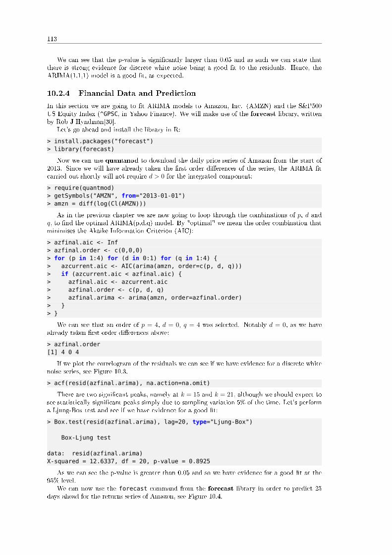
113

We can see that the p-value is signi�cantly larger than 0.05 and as such we can state thatthere is strong evidence for discrete white noise being a good �t to the residuals. Hence, theARIMA(1,1,1) model is a good �t, as expected.

10.2.4 Financial Data and Prediction

In this section we are going to �t ARIMA models to Amazon, Inc. (AMZN) and the S&P500US Equity Index (^GPSC, in Yahoo Finance). We will make use of the forecast library, writtenby Rob J Hyndman[30].

Let's go ahead and install the library in R:

> install.packages("forecast")> library(forecast)

Now we can use quantmod to download the daily price series of Amazon from the start of2013. Since we will have already taken the �rst order di�erences of the series, the ARIMA �tcarried out shortly will not require d > 0 for the integrated component:

> require(quantmod)> getSymbols("AMZN", from="2013-01-01")> amzn = diff(log(Cl(AMZN)))

As in the previous chapter we are now going to loop through the combinations of p, d andq, to �nd the optimal ARIMA(p,d,q) model. By "optimal" we mean the order combination thatminimises the Akaike Information Criterion (AIC):

> azfinal.aic <- Inf> azfinal.order <- c(0,0,0)> for (p in 1:4) for (d in 0:1) for (q in 1:4) {> azcurrent.aic <- AIC(arima(amzn, order=c(p, d, q)))> if (azcurrent.aic < azfinal.aic) {> azfinal.aic <- azcurrent.aic> azfinal.order <- c(p, d, q)> azfinal.arima <- arima(amzn, order=azfinal.order)> }> }

We can see that an order of p = 4, d = 0, q = 4 was selected. Notably d = 0, as we havealready taken �rst order di�erences above:

> azfinal.order[1] 4 0 4

If we plot the correlogram of the residuals we can see if we have evidence for a discrete whitenoise series, see Figure 10.3.

> acf(resid(azfinal.arima), na.action=na.omit)

There are two signi�cant peaks, namely at k = 15 and k = 21, although we should expect tosee statistically signi�cant peaks simply due to sampling variation 5% of the time. Let's performa Ljung-Box test and see if we have evidence for a good �t:

> Box.test(resid(azfinal.arima), lag=20, type="Ljung-Box")

Box-Ljung test

data: resid(azfinal.arima)X-squared = 12.6337, df = 20, p-value = 0.8925

As we can see the p-value is greater than 0.05 and so we have evidence for a good �t at the95% level.

We can now use the forecast command from the forecast library in order to predict 25days ahead for the returns series of Amazon, see Figure 10.4.

114

Figure 10.3: Correlogram of residuals of ARIMA(4,0,4) model �tted to AMZN daily log returns

> plot(forecast(azfinal.arima, h=25))

Figure 10.4: 25-day forecast of AMZN daily log returns

115

We can see the point forecasts for the next 25 days with 95% (dark blue) and 99% (lightblue) error bands. We will be using these forecasts in our �rst time series trading strategy whenwe come to combine ARIMA and GARCH later in the book.

Let's carry out the same procedure for the S&P500. Firstly we obtain the data from quantmodand convert it to a daily log returns stream:

> getSymbols("^GSPC", from="2013-01-01")> sp = diff(log(Cl(GSPC)))

We �t an ARIMA model by looping over the values of p, d and q:

> spfinal.aic <- Inf> spfinal.order <- c(0,0,0)> for (p in 1:4) for (d in 0:1) for (q in 1:4) {> spcurrent.aic <- AIC(arima(sp, order=c(p, d, q)))> if (spcurrent.aic < spfinal.aic) {> spfinal.aic <- spcurrent.aic> spfinal.order <- c(p, d, q)> spfinal.arima <- arima(sp, order=spfinal.order)> }> }

The AIC tells us that the "best" model is the ARIMA(2,0,1) model. Notice once again thatd = 0, as we have already taken �rst order di�erences of the series:

> spfinal.order[1] 2 0 1

We can plot the residuals of the �tted model to see if we have evidence of discrete whitenoise, see Figure 10.5.

> acf(resid(spfinal.arima), na.action=na.omit)

Figure 10.5: Correlogram of residuals of ARIMA(2,0,1) model �tted to S&P500 daily log returns

116

The correlogram looks promising, so the next step is to run the Ljung-Box test and con�rmthat we have a good model �t:

> Box.test(resid(spfinal.arima), lag=20, type="Ljung-Box")

Box-Ljung test

data: resid(spfinal.arima)X-squared = 13.6037, df = 20, p-value = 0.85

Since the p-value is greater than 0.05 we have evidence of a good model �t.

Why is it that in the previous chapter our Ljung-Box test for the S&P500 showed that theARMA(3,3) was a poor �t for the daily log returns?

Notice that I deliberately truncated the S&P500 data to start from 2013 onwards here, whichconveniently excludes the volatile periods around 2007-2008. Hence we have excluded a largeportion of the S&P500 where we had excessive volatility clustering. This impacts the serialcorrelation of the series and hence has the e�ect of making the series seem "more stationary"than it has been in the past.

This is a very important point. When analysing time series we need to be extremely carefulof conditionally heteroscedastic series, such as stock market indexes. In quantitative �nance,trying to determine periods of di�ering volatility is often known as "regime detection". It is oneof the harder tasks to achieve!

Let's now plot a forecast for the next 25 days of the S&P500 daily log returns, see Figure10.6.

> plot(forecast(spfinal.arima, h=25))

Figure 10.6: 25-day forecast of S&P500 daily log returns

Now that we have the ability to �t and forecast models such as ARIMA, we're very close tobeing able to create strategy indicators for trading.

117

10.2.5 Next Steps

In the next section we are going to take a look at the Generalised Autoregressive ConditionalHeteroscedasticity (GARCH) model and use it to explain more of the serial correlation in certainequities and equity index series.

Once we have discussed GARCH we will be in a position to combine it with the ARIMAmodel and create signal indicators and thus a basic quantitative trading strategy.

10.3 Volatility

The main motivation for studying conditional heteroskedasticity in �nance is that of volatilityof asset returns. Volatility is an incredibly important concept in �nance because it is highlysynonymous with risk.

Volatility has a wide range of applications in �nance:

� Options Pricing - The Black-Scholes model for options prices is dependent upon thevolatility of the underlying instrument

� Risk Management - Volatility plays a role in calculating the VaR of a portfolio, theSharpe Ratio for a trading strategy and in determination of leverage

� Tradeable Securities - Volatility can now be traded directly by the introduction of theCBOE Volatility Index (VIX), and subsequent futures contracts and ETFs

Hence, if we can e�ectively forecast volatility then we will be able to price options moreaccurately, create more sophisticated risk management tools for our algorithmic trading portfoliosand even come up with new strategies that trade volatility directly.

We're now going to turn our attention to conditional heteroskedasticity and discuss what itmeans.

10.4 Conditional Heteroskedasticity

Let's �rst discuss the concept of heteroskedasticity and then examine the "conditional" part.If we have a collection of random variables, such as elements in a time series model, we say

that the collection is heteroskedastic if there are certain groups, or subsets, of variables withinthe larger set that have a di�erent variance from the remaining variables.

For instance, in a non-stationary time series that exhibits seasonality or trending e�ects, wemay �nd that the variance of the series increases with the seasonality or the trend. This form ofregular variability is known as heteroskedasticity.

However, in �nance there are many reasons why an increase in variance is correlated to afurther increase in variance.

For instance, consider the prevalence of downside portfolio protection insurance employedby long-only fund managers. If the equities markets were to have a particularly challengingday (i.e. a substantial drop!) it could trigger automated risk management sell orders, whichwould further depress the price of equities within these portfolios. Since the larger portfolios aregenerally highly correlated anyway, this could trigger signi�cant downward volatility.

These "sell-o�" periods, as well as many other forms of volatility that occur in �nance, leadto heteroskedasticity that is serially correlated and hence conditional on periods of increasedvariance. Thus we say that such series are conditional heteroskedastic.

One of the challenging aspects of conditional heteroskedastic series is that if we were to plotthe correlogram of a series with volatility we might still see what appears to be a realisationof stationary discrete white noise. That is, the volatility itself is hard to detect purely fromthe correlogram. This is despite the fact that the series is most de�nitely non-stationary as itsvariance is not constant in time.

We are going to describe a mechanism for detecting conditional heteroskedastic series in thischapter and then use the ARCH and GARCH models to account for it, ultimately leading tomore realistic forecasting performance, and thus more pro�table trading strategies.

118

10.5 Autoregressive Conditional Heteroskedastic Models

We've now discussed conditional heteroskedasticity (CH) and its importance within �nancialseries. We want a class of models that can incorporate CH in a natural way. We know that theARIMA model does not account for CH, so how can we proceed?

Well, how about a model that utilises an autoregressive process for the variance itself? Thatis, a model that actually accounts for the changes in the variance over time using past values ofthe variance.

This is the basis of the Autoregressive Conditional Heteroskedastic (ARCH) model. We'llbegin with the simplest possible case, namely an ARCHmodel that depends solely on the previousvariance value in the series.

10.5.1 ARCH De�nition

De�nition 10.5.1. Autoregressive Conditional Heteroskedastic Model of Order Unity.A time series {εt} is given at each instance by:

εt = σtwt (10.5)

Where {wt} is discrete white noise, with zero mean and unit variance, and σ2t is given by:

σ2t = α0 + α1ε

2t−1 (10.6)

Where α0 and α1 are parameters of the model.We say that {εt} is an autoregressive conditional heteroskedastic model of order unity, denoted

by ARCH(1). Substituting for σ2t , we receive:

εt = wt

√α0 + α1ε2t−1 (10.7)

10.5.2 Why Does This Model Volatility?

I personally �nd the above "formal" de�nition lacking in motivation as to how it introducesvolatility. However, you can see how it is introduced by squaring both sides of the previousequation:

Var(εt) = E[ε2t ]− (E[εt])2 (10.8)

= E[ε2t ] (10.9)

= E[w2t ] E[α0 + α1ε

2t−1] (10.10)

= E[α0 + α1ε2t−1] (10.11)

= α0 + α1 Var(εt−1) (10.12)

Where I have used the de�nitions of the variance Var(x) = E[x2]− (E[x])2 and the linearityof the expectation operator E, along with the fact that {wt} has zero mean and unit variance.

Thus we can see that the variance of the series is simply a linear combination of the varianceof the prior element of the series. Simply put, the variance of an ARCH(1) process follows anAR(1) process.

It is interesting to compare the ARCH(1) model with an AR(1) model. Recall that the latteris given by:

xt = α0 + α1xt−1 + wt (10.13)

You can see that the models are similar in form (with the exception of the white noise term).

119

10.5.3 When Is It Appropriate To Apply ARCH(1)?

So what approach can we take in order to determine whether an ARCH(1) model is appropriateto apply to a series?

Consider that when we were attempting to �t an AR(1) model we were concerned with thedecay of the �rst lag on a correlogram of the series. However, if we apply the same logic to thesquare of the residuals, and see whether we can apply an AR(1) to these squared residuals thenwe have an indication that an ARCH(1) process may be appropriate.

Note that ARCH(1) should only ever be applied to a series that has already had an appropriatemodel �tted su�cient to leave the residuals looking like discrete white noise. Since we can only tellwhether ARCH is appropriate or not by squaring the residuals and examining the correlogram,we also need to ensure that the mean of the residuals is zero.

Crucially, ARCH should only ever be applied to series that do not have any trends or seasonale�ects, i.e. that has no (evident) serial correlation. ARIMA is often applied to such a series (oreven Seasonal ARIMA), at which point ARCH may be a good �t.

10.5.4 ARCH(p) Models

It is straightforward to extend ARCH to higher order lags. An ARCH(p) process is given by:

εt = wt

√√√√α0 +

p∑i=1

αpε2t−i (10.14)

You can think of ARCH(p) as applying an AR(p) model to the variance of the series.An obvious question to ask at this stage is if we are going to apply an AR(p) process to

the variance, why not a Moving Average MA(q) model as well? Or a mixed model such asARMA(p,q)?

This is actually the motivation for the Generalised ARCH model, known as GARCH, whichwe will now de�ne and discuss.

10.6 Generalised Autoregressive Conditional Heteroskedas-tic Models

10.6.1 GARCH De�nition

De�nition 10.6.1. Generalised Autoregressive Conditional Heteroskedastic Model of Order p,q.

A time series {εt} is given at each instance by:

εt = σtwt (10.15)

Where {wt} is discrete white noise, with zero mean and unit variance, and σ2t is given by:

σ2t = α0 +

q∑i=1

αiε2t−i +

p∑j=1

βjσ2t−j (10.16)

Where αi and βj are parameters of the model.We say that {εt} is a generalised autoregressive conditional heteroskedastic model of order

p,q, denoted by GARCH(p,q).

Hence this de�nition is similar to that of ARCH(p), with the exception that we are addingmoving average terms, that is the value of σ2 at t, σ2

t , is dependent upon previous σ2t−j values.

Thus GARCH is the "ARMA equivalent" of ARCH, which only has an autoregressive com-ponent.

120

10.6.2 Simulations, Correlograms and Model Fittings

As always we're going to begin with the simplest possible case of the model, namely GARCH(1,1).This means we are going to consider a single autoregressive lag and a single "moving average"lag. The model is given by the following:

εt = σtwt (10.17)

σ2t = α0 + α1ε

2t−1 + β1σ

2t−1 (10.18)

Note that it is necessary for α1 + β1 < 1 otherwise the series will become unstable.We can see that the model has three parameters, namely α0, α1 and β1. Let's set α0 = 0.2,

α1 = 0.5 and β1 = 0.3.To create the GARCH(1,1) model in R we need to perform a similar procedure as for our

original random walk simulations. That is, we need to create a vector w to store our randomwhite noise values, then a separate vector eps to store our time series values and �nally a vectorsigsq to store the ARMA variances.

We can use the R rep command to create a vector of zeros that we will populate with ourGARCH values:

> set.seed(2)> a0 <- 0.2> a1 <- 0.5> b1 <- 0.3> w <- rnorm(10000)> eps <- rep(0, 10000)> sigsq <- rep(0, 10000)> for (i in 2:10000) {> sigsq[i] <- a0 + a1 * (eps[i-1]^2) + b1 * sigsq[i-1]> eps[i] <- w[i]*sqrt(sigsq[i])> }

At this stage we have generated our GARCH model using the aforementioned parametersover 10,000 samples. We are now in a position to plot the correlogram, which is given in Figure10.7.

> acf(eps)

Notice that the series looks like a realisation of a discrete white noise process.However, if we plot correlogram of the square of the series, as given in Figure 10.8,

> acf(eps^2)

we see substantial evidence of a conditionally heteroskedastic process via the decay of suc-cessive lags.

As in the previous chapter we now want to try and �t a GARCH model to this simulatedseries to see if we can recover the parameters. Thankfully, a helpful library called tseriesprovides the garch command to carry this procedure out:

> require(tseries)

We can then use the confint command to produce con�dence intervals at the 97.5% levelfor the parameters:

> eps.garch <- garch(eps, trace=FALSE)> confint(eps.garch)

2.5 % 97.5 %a0 0.1786255 0.2172683a1 0.4271900 0.5044903b1 0.2861566 0.3602687

We can see that the true parameters all fall within the respective con�dence intervals.

121

Figure 10.7: Correlogram of a simulated GARCH(1,1) model with α0 = 0.2, α1 = 0.5 andβ1 = 0.3

Figure 10.8: Correlogram of a simulated GARCH(1,1) models squared values with α0 = 0.2,α1 = 0.5 and β1 = 0.3

122

10.6.3 Financial Data

Now that we know how to simulate and �t a GARCH model, we want to apply the procedure tosome �nancial series. In particular, let's try �tting ARIMA and GARCH to the FTSE 100 indexof the largest UK companies by market capitalisation. Yahoo Finance uses the symbol ^FTSEfor the index. We can use quantmod to obtain the data:

> require(quantmod)> getSymbols("^FTSE")

We can then calculate the di�erences of the log returns of the closing price:

> ftrt = diff(log(Cl(FTSE)))

Let's plot the values, as given in Figure 10.9.

> plot(ftrt)

It is very clear that there are periods of increased volatility, particularly around 2008-2009,late 2011 and more recently in mid 2015:

Figure 10.9: Di�erenced log returns of the daily closing price of the FTSE 100 UK stock index

We also need to remove the NA value generated by the di�erencing procedure:

> ft <- as.numeric(ftrt)> ft <- ft[!is.na(ft)]

The next task is to �t a suitable ARIMA(p,d,q) model. We saw how to do that in the previouschapter, so I won't repeat the procedure here, I will simply provide the code:

> ftfinal.aic <- Inf> ftfinal.order <- c(0,0,0)> for (p in 1:4) for (d in 0:1) for (q in 1:4) {> ftcurrent.aic <- AIC(arima(ft, order=c(p, d, q)))> if (ftcurrent.aic < ftfinal.aic) {> ftfinal.aic <- ftcurrent.aic

123

> ftfinal.order <- c(p, d, q)> ftfinal.arima <- arima(ft, order=ftfinal.order)> }> }

Since we've already di�erenced the FTSE returns once, we should expect our integratedcomponent d to equal zero, which it does:

> ftfinal.order[1] 4 0 4

Thus we receive an ARIMA(4,0,4) model, that is four autoregressive parameters and fourmoving average parameters.

We are now in a position to decide whether the residuals of this model �t possess evidenceof conditional heteroskedastic behaviour. To test this we need to plot the correlogram of theresiduals, as given in Figure 10.10.

> acf(resid(ftfinal.arima))

Figure 10.10: Residuals of an ARIMA(4,0,4) �t to the FTSE100 di� log returns

This looks like a realisation of a discrete white noise process indicating that we have achieveda good �t with the ARIMA(4,0,4) model.

To test for conditional heteroskedastic behaviour we need to square the residuals and plotthe corresponding correlogram, as given in Figure 10.11.

> acf(resid(ftfinal.arima)^2)

We can see clear evidence of serial correlation in the squared residuals, leading us to theconclusion that conditional heteroskedastic behaviour is present in the di� log return series ofthe FTSE100.

We are now in a position to �t a GARCH model using the tseries library.The �rst command actually �ts an appropriate GARCH model, with the trace=F parameter

telling R to suppress excessive output.The second command removes the �rst element of the residuals, since it is NA:

124

Figure 10.11: Squared residuals of an ARIMA(4,0,4) �t to the FTSE100 di� log returns

> ft.garch <- garch(ft, trace=F)> ft.res <- ft.garch$res[-1]

Finally, to test for a good �t we can plot the correlogram of the GARCH residuals and thesquare GARCH residuals, as given in Figure 10.12.

> acf(ft.res)

The correlogram looks like a realisation of a discrete white noise process, indicating a good�t. Let's now try the squared residuals, given in Figure 10.13.

> acf(ft.res^2)

Once again, we have what looks like a realisation of a discrete white noise process, indi-cating that we have "explained" the serial correlation present in the squared residuals with anappropriate mixture of ARIMA(p,d,q) and GARCH(p,q).

10.7 Next Steps

We are now at the point in our time series education where we have studied ARIMA and GARCH,allowing us to �t a combination of these models to a stock market index, and to determine if wehave achieved a good �t or not.

The next step is to actually produce forecasts of future daily returns values from this com-bination and use it to create a basic trading strategy. We will discuss this in the QuantitativeTrading Strategies part of the book.

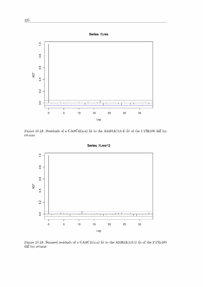
125

Figure 10.12: Residuals of a GARCH(p,q) �t to the ARIMA(4,0,4) �t of the FTSE100 di� logreturns

Figure 10.13: Squared residuals of a GARCH(p,q) �t to the ARIMA(4,0,4) �t of the FTSE100di� log returns

126

Chapter 11

State Space Models and the KalmanFilter

Thus far in our analysis of time series we have considered linear time series models includingARMA, ARIMA as well as the GARCH model for conditional heteroskedasticity. In this chapterwe are going to consider a more general class of models known as state space models, theprimary bene�t of which is that unlike the ARIMA family, their parameters can adapt over time.

State space models are very general and it is possible to put the models we have consideredto date into a state space formulation. However, in order to keep the analysis straightforward,it is often better to use the simpler representation.

The general premise of a state space model is that we have a set of states that evolve intime (such as the hedge ratio between two cointegrated pairs of equities), but our observationsof these states contain statistical noise (such as market microstructure noise), and hence we areunable to ever directly observe the "true" states.

The goal of the state space model is to infer information about the states, given the obser-vations, as new information arrives. A famous algorithm for carrying out this procedure is theKalman Filter, which we will also discuss in this article.

The Kalman Filter is ubiquitous in engineering control problems, including guidance & navi-gation, spacecraft trajectory analysis and manufacturing, but it is also widely used in quantitative�nance.

In engineering, for instance, a Kalman Filter will be used to estimate values of the state,which are then used to control the system under study. This introduces a feedback loop, oftenin real-time.

Perhaps the most common usage of a Kalman Filter in quantitative trading is to updatehedging ratios between assets in a statistical arbitrage pairs trade, but the algorithm is muchmore general than this and we will look at other use cases.

Generally, there are three types of inference that we are interested in when considering statespace models:

� Prediction - Forecasting subsequent values of the state

� Filtering - Estimating the current values of the state from past and current observations

� Smoothing - Estimating the past values of the state given the observations

Filtering and smoothing are similar, but not the same. Perhaps the best way to think of thedi�erence is that with smoothing we are really wanting to understand what has happened tostates in the past given our current knowledge, whereas with �ltering we really want to knowwhat is happening with the state right now.

In this chapter we are going to discuss the theory of the state space model and how we canuse the Kalman Filter to carry out the various types of inference described above. We will thenapply the Kalman Filter to trading situations, such as cointegrated pairs, as well as asset priceprediction, later in the book.

127

128

We will be making use of a Bayesian approach to the problem, as this is a natural statisticalframework for allowing us to readily update our beliefs in light of new information, which isprecisely the desired behaviour of the Kalman Filter.

I want to warn you that state-space models and Kalman Filters su�er from an abundance ofmathematical notation, even if the conceptual ideas behind them are relatively straightforward.I will try and explain all of this notation in depth, as it can be confusing for those new toengineering control problems or state-space models in general. Fortunately we will be letting Rdo the heavy lifting of solving the model for us, so the verbose notation will not be a problem inpractice.

11.1 Linear State-Space Model

Let's begin by discussing all of the elements of the linear state-space model.Since the states of the system are time-dependent, we need to subscript them with t. We

will use θt to represent a column vector of the states.In a linear state-space model we say that these states are a linear combination of the prior

state at time t− 1 as well as system noise (random variation). In order to simplify the analysiswe are going to suggest that this noise is drawn from a multivariate normal distribution, but ofcourse, other distributions can be used.

The linear dependence of θt on the previous state θt−1 is given by the matrix Gt, which canalso be time-varying (hence the subscript t). The multivariate time-dependent noise is given bywt. The relationship is summarised below in what is often called the state equation:

θt = Gtθt−1 + wt (11.1)

However, this is only half of the story. We also need to discuss the observations, that is, whatwe actually see, since the states are hidden to us by system noise.

We can denote the (time-dependent) observations by yt. The observations are a linear combi-nation of the current state and some additional random variation known as measurement noise,also drawn from a multivariate normal distribution.

If we denote the linear dependence matrix of θt on yt by Ft (also time-dependent), and themeasurement noise by vt we have the observation equation:

yt = FTt θt + vt (11.2)

Where FT is the transpose of F .In order to fully specify the model we need to provide the �rst state θ0, as well as the variance-

covariance matrices for the system noise and measurement noise. These terms are distributedas:

θ0 ∼ N (m0, C0) (11.3)

vt ∼ N (0, Vt) (11.4)

wt ∼ N (0,Wt) (11.5)

Clearly that is a lot of notation to specify the model. For completeness, I'll summarise all ofthe terms here to help you get to grips with the model:

� θt - The state of the model at time t

� yt - The observation of the model at time t

� Gt - The state-transition matrix between current and prior states at time t and t − 1respectively

129

� Ft - The observation matrix between the current observation and current state at timet

� wt - The system noise drawn from a multivariate normal distribution

� vt - The measurement noise drawn from a multivariate normal distribution

� m0 - The mean value of the multivariate normal distribution of the initial state, θ0

� C0 - The variance-covariance matrix of the multivariate normal distribution of the initialstate, θ0

� Wt - The variance-covariance matrix for the multivariate normal distribution from whichthe system noise is drawn

� Vt - The variance-covariance matrix for the multivariate normal distribution from fromwhich the measurement noise is drawn

Now that we've speci�ed the linear state-space model, we need an algorithm to actually solveit. This is where the Kalman Filter comes in. We can use Bayes' Rule and conjugate priors, asdiscussed in the previous part of the book, to help us derive the algorithm.

11.2 The Kalman Filter

This section follows very closely the notation and analysis carried out in Pole et al[40]. I decidedit wasn't particularly helpful to invent my own notation for the Kalman Filter, as I want you tobe able to relate it to other research papers or texts.

11.2.1 A Bayesian Approach

If we recall from the prior chapters on Bayesian inference, Bayes' Rule is given by:

P (θ|D) = P (D|θ)P (θ)/P (D) (11.6)

Where θ refers to our parameters and D refers to our data or observations.We want to apply the rule to the idea of updating the probability of seeing a state given all of

the previous data we have and our current observation. Once again, we need to introduce morenotation!

If we are at time t, then we can represent all of the data known about the system by thequantity Dt. However, our current observations are given by yt. Thus we can say that Dt =(Dt−1, yt). That is, our current knowledge is a mixture of our previous knowledge plus our mostrecent observation.

Applying Bayes' Rule to this situation gives the following:

P (θt|Dt−1, yt) =P (yt|θt)P (θt|Dt−1)

P (yt)(11.7)

What does this mean? It says that the posterior or updated probability of obtaining a stateθt, given our current observation yt and previous data Dt−1, is equal to the likelihood of seeingan observation yt, given the current state θt multiplied by the prior or previous belief of thecurrent state, given only the previous data Dt−1, normalised by the probability of seeing theobservation yt regardless.

While the notation may be somewhat verbose, it is a very natural statement. It says thatwe can update our view on the state, θt, in a rational manner given the fact that we have newinformation in the form of the current observation, yt.

One of the extremely useful aspects of Bayesian inference is that if our prior and likelihood areboth normally distributed, we can use the concept of conjugate priors to state that our posterior(i.e. updated view of θt) will also be normally distributed.

130

We utilised the same concept, albeit with di�erent distributional forms, in our previousdiscussion on the inference of binomial proportions.

So how does this help us produce a Kalman Filter?Well, let's specify the terms that we'll be using, from Bayes' Rule above. Firstly, we specify

the distributional form of the prior:

θt|Dt−1 ∼ N (at, Rt) (11.8)

That is, the prior view of θ at time t, given our knowledge at time t − 1 is distributed asa multivariate normal distribution, with mean at and variance-covariance Rt. The latter twoparameters will be de�ned below.

Now let's consider the likelihood:

yt|θt ∼ N (FTt θt, Vt) (11.9)

That is, the likelihood function of the current observation y at time t is distributed as amultivariate normal distribution, with mean FTt θt and variance-covariance Vt. We've alreadyoutlined these terms in our list above.

Finally we have the posterior of θt:

θt|Dt ∼ N (mt, Ct) (11.10)

That is, our posterior view of the current state θ at time t, given our current knowledge attime t is distributed as a multivariate normal distribution with mean mt and variance-covarianceCt.

The Kalman Filter is what links all of these terms together for t = 1, . . . , n. We won't derivewhere these values actually come from, but we will simply state them. Thankfully we can uselibrary implementations in R to carry out the "heavy lifting" for us:

at = Gtmt−1 (11.11)

Rt = GtCt−1GTt +Wt (11.12)

et = yt − ft (11.13)

mt = at +Atet (11.14)

ft = FTt at (11.15)

Qt = FTt RtFt + Vt (11.16)

At = RtFtQ−1t (11.17)

Ct = Rt −AtQtATt (11.18)

Clearly that is a lot of notation! As I said above, we need not worry about the excessiveverboseness of the Kalman Filter, as we can simply use libraries in R to calculate the algorithmfor us.

So how does it all �t together? Well, ft is the predicated value of the observation at time t,where we make this prediction at time t− 1. Since et = yt − ft, we can see easily that et is theerror associated with the forecast (the di�erence between f and y).

Importantly, the posterior mean is a weighting of the prior mean and the forecast error, sincemt = at +Atet = Gtmt−1 +Atet, where Gt and At are our weighting matrices.

Now that we have an algorithmic procedure for updating our views on the observations andstates, we can use it to make predictions, as well as smooth the data.

11.2.2 Prediction

The Bayesian approach to the Kalman Filter leads naturally to a mechanism for prediction.Since we have our posterior estimate for the state θt, we can predict the next day's values byconsidering the mean value of the observation.

131

Let's take the expected value of the observation tomorrow, given our knowledge of the datatoday :

E[yt+1|Dt] = E[FTt+1θt + vt+1|Dt] (11.19)

= FTt+1E[θt+1|Dt] (11.20)

= FTt+1at+1 (11.21)

= ft+1 (11.22)

Where does this come from? Let's try and follow through the analysis:Since the likelihood function for today's observation yt, given today's state θt, is normally

distributed with mean FTt θt and variance-covariance Vt (see above), we have that the expectationof tomorrow's observation yt+1, given our data today, Dt, is precisely the expectation of themultivariate normal for the likelihood, namely E[FTt+1θt+vt+1|Dt]. Once we make this connectionit simply reduces to applying rules about the expectation operator to the remaining matricesand vectors, ultimately leading us to ft+1.

However it is not su�cient to simply calculate the mean, we must also know the variance oftomorrow's observation given today's data, otherwise we cannot truly characterise the distribu-tion on which to draw tomorrow's prediction.

Var[yt+1|Dt] = Var[FTt+1θt + vt+1|Dt] (11.23)

= FTt+1 Var[θt+1|Dt]Ft+1 + Vt+1 (11.24)

= FTt+1Rt+1Ft+1 + Vt+1 (11.25)

= Qt+1 (11.26)

Now that we have the expectation and variance of tomorrow's observation, given today'sdata, we are able to provide the general forecast for k steps ahead, by fully characterising thedistribution on which these predictions are drawn:

yt+k|Dt ∼ N (ft+k|t, Qt+k|t) (11.27)

Note that I have used some odd notation here - what does it mean to have a subscript oft+ k|t? Actually, it allows us to write a convenient shorthand for the following:

ft+k|t = FTt+kGk−1at+1 (11.28)

Qt+k|t = FTt+kRt+kFt+k + Vt+k (11.29)

Rt+k|t = Gk−1Rt+1(Gk−1)T +

k∑j=2

Gk−jWt+j(Gk−j)T (11.30)

As I've mentioned repeatedly in this chapter, we should not concern ourselves too much withthe verboseness of the Kalman Filter and its notation, rather we should think about the overallprocedure and its Bayesian underpinnings.

Thus we now have the means of predicting new values of the series. This is an alternativeto the predictions produced by combining ARIMA and GARCH. In subsequent chapters later inthe book we will actually carry this out for some real �nancial data and apply it to a predictivetrading model.

We will also be able to use the "�lter" aspect to provide us with continually updated viewson a linear hedge ratio between two cointegrated pairs of assets, such as might be found in astastical arbitrage strategy.

132

Part IV

Statistical Machine Learning

133

Chapter 12

Model Selection andCross-Validation

In this chapter I want to discuss one of the most important and tricky issues in machine learning,that of model selection and the bias-variance tradeo�. The latter is one of the most crucial issuesin helping us achieve pro�table trading strategies based on machine learning techniques.

Model selection refers to our ability to assess performance of di�ering machine learningmodels in order to choose the best one.

The bias-variance tradeo� is a particular property of all (supervised) machine learningmodels, that enforces a tradeo� between how "�exible" the model is and how well it performson unseen data. The latter is known as a models generalisation performance.

12.1 Bias-Variance Trade-O�

We will begin by understanding why model selection is important and then discuss the bias-variance tradeo� qualitatively. We will wrap up the chapter by deriving the bias-variance tradeo�mathematically and discuss measures to minimise the problems it introduces.

In this chapter we are considering supervised regression models. That is, models which aretrained on a set of labelled training data and produce a quantitative response. An example ofthis would be attempting to predict future stock prices based on other factors such as past prices,interest rates or foreign exchange rates.

This is in contrast to a categorical or binary response model as in the case of supervisedclassi�cation. An example of a classi�cation setting would be attempting to assign a topic to atext document, from a �nite set of topics. The bias-variance and model selection situations forclassi�cation are extremely similar to the regression setting and simply require modi�cation tohandle the di�ering ways in which errors and performance are measured.

12.1.1 Machine Learning Models

As with most of our discussions in machine learning the basic model is given by the following:

Y = f(X) + ε (12.1)

This states that the response vector, Y , is given as a (potentially non-linear) function, f , ofthe predictor vector, X, with a set of normally distributed error terms that have mean zero anda standard deviation of one.

What does this mean in practice?As an example, our vector X could represent a set of lagged �nancial prices, similar to the

time series autoregressive models we considered earlier in the book. It could also representinterest rates, derivatives prices, real-estate prices, word-frequencies in a document or any otherfactor that we consider useful in making a prediction.

135

136

The vector Y could be single or multi-valued. In the former case it might simply representtomorrow's stock price, in the latter case it might represent the next week's daily predictedprices.

f represents our view on the underlying relationship between Y and X. This could be linear,in which case we may estimate f via a linear regression model. It may be non-linear, in whichcase we may estimate f with a Support Vector Machine or a spline-based method, for instance.

The error terms ε represent all of the factors that a�ect Y that we haven't taken into accountwith our function f . They are essentially the "unknown" components of our prediction model.It is commmon to assume that these are normally distributed with mean zero and a standarddeviation of one.

In this section we are going to describe how to measure the performance of an estimatefor the (unknown) function f . As with the time series models discussed previously, such an

estimate uses "hat" notation. Hence, f can be read as "the estimate of f".In addition we will describe the e�ect on the performance of the model as we make it more

�exible. Flexibility describes the ability to increase the degrees of freedom available to the modelto "�t" to the training data. We will see that the relationship between �exibility and performanceerror is non-linear and thus we need to be extremely careful when choosing the "best" model.

Note that there is never a "best" model across the entirety of statistics, time series or machinelearning. Di�erent models have varying strengths and weaknesses. One model may workvery well on one dataset, but may perform badly on another. The challenge in statistical machinelearning is to pick the "best" model for the problem at hand with the data available.

12.1.2 Model Selection

When trying to ascertain which statistical machine learning method is best we need some means ofcharacterising the relative performance between models. In the time series section we consideredthe Akaike Information Criterion and the Bayesian Information Criterion. In this section we willconsider other methods.

To determine model suitability we need to compare the known values of the underlying rela-tionship with those that are predicted by an estimated model.

For instance, if we are attempting to predict tomorrow's stock prices, then we wish to evaluatehow close our models predictions are to the true value on that particular day.

This motivates the concept of a loss function, which quantitatively compares the di�erencebetween the true values with the predicted values.

Let's assume that we have created an estimate f of the underlying relationship f . f mightbe a linear regression or a Random Forest model, for instance. f will have been trained on aparticular data set, τ , which contains predictor-response pairs. If there are N such pairs then τis given by:

τ = {(X1, Y1), ..., (XN , YN )} (12.2)

The Xi represent the prediction factors, which could be prior lagged prices for a series orsome other factors, as mentioned above. The Yi could be the predictions for our stock prices inthe following period. In this instance, N represents the number of days of data that we haveavailable.

The loss function is denoted by L(Y, f(X)). Its job is to compare the predictions made by fat particular values of X to their true values given by Y . A common choice for L is the absoluteerror :

L(Y, f(X)) = |Y − f(X)| (12.3)

Another popular choice is the squared error :

L(Y, f(X)) = (Y − f(X))2 (12.4)

137

Note that both choices of loss function are non-negative. Hence the "best" loss for a modelis zero, that is, there is no di�erence between the prediction and the true value.

Training Error versus Test Error

Now that we have a loss function we need some way of aggregating the various di�erences betweenthe true values and the predicted values. One way to do this is to de�ne the Mean SquaredError (MSE), which is simply the average, or expectation value, of the squared loss:

MSE :=1

N

N∑i=1

(Yi − f(Xi))2 (12.5)

The de�nition simply states that the Mean Squared Error is the average of all of the squareddi�erences between the true values Yi and the predicted values f(Xi). A smaller MSE meansthat the estimate is more accurate.

It is important to realise that this MSE value is computed using only the training data. Thatis, it is computed using only the data that the model was �tted on. Hence, it is actually knownas the training MSE.

In practice this value is of little interest to us. What we are really concerned about is howwell the model can predict values on new unseen data.

For instance, we are not really interested in how well the model can predict past stock pricesof the following day, we are only concerned with how it can predict the following days stockprices going forward. This quanti�cation of a models performance is known as its generalisationperformance. It is what we are really interested in.

Mathematically, if we have a new prediction value X0 and a true response Y0, then we wishto take the expectation across all such new values to come up with the test MSE:

Test MSE := E[(Y0 − f(X0))2

](12.6)

Where the expectation is taken across all new unseen predictor-response pairs (X0, Y0).Our goal is to select the model where the test MSE is lowest across choices of other models.Unfortunately it is di�cult to calculate the test MSE! This is because we are often in a

situation where we do not have any test data available.In general machine learning domains this can be quite common. In quantitative trading we

are (usually) in a "data rich" environment and thus we can retain some of our data for trainingand some for testing. In the next section we will discuss cross-validation, which is one means ofutilising subsets of the training data in order to estimate the test MSE.

A pertinent question to ask at this stage is "Why can we not simply use the model withthe lowest training MSE?". The simple answer is that there is no guarantee that the modelwith the lowest training MSE will also be the model with the lowest test MSE. Why is this so?The answer lies in a particular property of statistical machine learning methods known as thebias-variance tradeo�.

12.1.3 The Bias-Variance Tradeo�

Let's consider a slightly contrived situation where we know the underlying "true" relationshipbetween Y and X, which I will state is given by a sinusoidal function, f = sin, such thatY = f(X) = sin(X). Note that in reality we will not ever know the underlying f , which is whywe are estimating it in the �rst place!

For this contrived situation I have created a set of training points, τ , given by Yi = sin(Xi)+εi,where εi are draws from a standard normal distribution (mean of zero, standard deviation equalto one). This can be seen in Figure 12.1. The black curve is the "true" function f , restricted tothe interval [0, 2π], while the circled points represent the Yi simulated data values.

We can now try to �t a few di�erent models to this training data. The �rst model, given bythe green line, is a linear regression �tted with ordinary least squares estimation. The second

138

Figure 12.1: Various estimates of the underlying sinusoidal model, f = sin

model, given by the blue line, is a polynomial model with degree m = 3. The third model, givenby the red curve is a higher degree polynomial with degree m = 20. Between each of the modelsI have varied the �exibility, that is, the degrees of freedom (DoF). The linear model is the least�exible with only two DoF. The most �exible model is the polynomial of order m = 20. It can beseen that the polynomial of order m = 3 is the apparent closest �t to the underlying sinusoidalrelationship.

For each of these models we can calculate the training MSE. It can be seen in Figure 12.2that the training MSE (given by the green curve) decreases monotonically as the �exibility of themodel increases. This makes sense, since the polynomial �t can become as �exible as we need itto in order to minimise the di�erence between its values and those of the sinusoidal data.

However, if we plot the test MSE (given by the blue curve) the situation is vastly di�erent.The test MSE initially decreases as we increase the �exibility of the model but eventually startsto increase again after we introduce a lot of �exibility. Why is this? By allowing the model tobe extremely �exible we are letting it �t to "patterns" in the training data.

However, as soon as we introduce new unseen data points in the test set the model cannotgeneralise well because these "patterns" are only random artifacts of the training data and arenot an underlying property of the true sinusoidal form. We are in a situation of over�tting.

In fact, this property of a "u-shaped" test MSE as a function of model �exibility is an intrinsicproperty of statistical machine learning models, known as the bias-variance tradeo�.

It can be shown (see below in the Mathematical Explanation section) that the expected testMSE, where the expectation is taken across many training sets, is given by:

E(Y0 − f(X0))2 = Var(f(X0)) +[Biasf(X0)

]2+ Var(ε) (12.7)

The �rst term on the right hand side is the variance of the estimate across many trainingsets. It determines how much the average model estimation deviates as di�erent training dataare tried. In particular, a model with high variance is suggestive that it is over�t to the trainingdata.

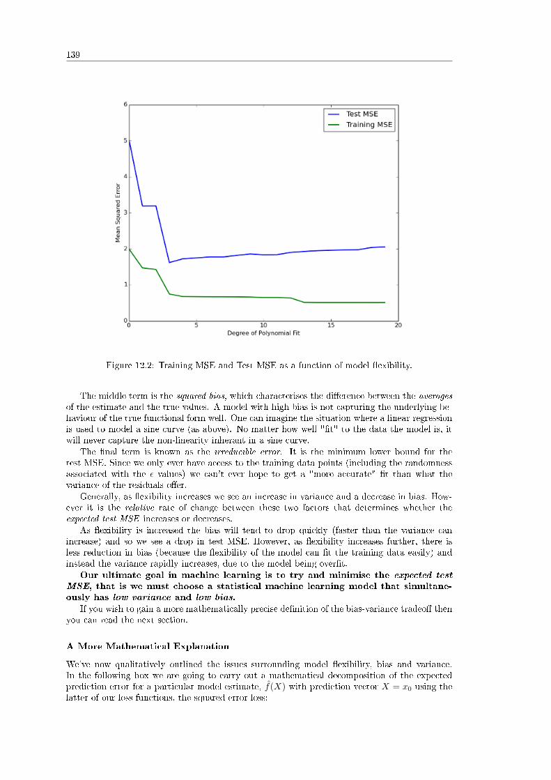
139

Figure 12.2: Training MSE and Test MSE as a function of model �exibility.

The middle term is the squared bias, which characterises the di�erence between the averagesof the estimate and the true values. A model with high bias is not capturing the underlying be-haviour of the true functional form well. One can imagine the situation where a linear regressionis used to model a sine curve (as above). No matter how well "�t" to the data the model is, itwill never capture the non-linearity inherant in a sine curve.

The �nal term is known as the irreducible error. It is the minimum lower bound for thetest MSE. Since we only ever have access to the training data points (including the randomnessassociated with the ε values) we can't ever hope to get a "more accurate" �t than what thevariance of the residuals o�er.

Generally, as �exibility increases we see an increase in variance and a decrease in bias. How-ever it is the relative rate of change between these two factors that determines whether theexpected test MSE increases or decreases.

As �exibility is increased the bias will tend to drop quickly (faster than the variance canincrease) and so we see a drop in test MSE. However, as �exibility increases further, there isless reduction in bias (because the �exibility of the model can �t the training data easily) andinstead the variance rapidly increases, due to the model being over�t.

Our ultimate goal in machine learning is to try and minimise the expected test

MSE, that is we must choose a statistical machine learning model that simultane-ously has low variance and low bias.

If you wish to gain a more mathematically precise de�nition of the bias-variance tradeo� thenyou can read the next section.

A More Mathematical Explanation

We've now qualitatively outlined the issues surrounding model �exibility, bias and variance.In the following box we are going to carry out a mathematical decomposition of the expectedprediction error for a particular model estimate, f(X) with prediction vector X = x0 using thelatter of our loss functions, the squared-error loss:

140

The de�nition of the squared error loss, at the prediction point X0, is given by:

Err(X0) = E[(Y − f(X0)

)2

|X = X0

](12.8)

However, we can expand the expectation on the right hand side into three terms:

Err(X0) = σ2ε +

[Ef(X0)− f(X0)

]2+ E

[f(X0)− Ef(X0)

]2(12.9)

The �rst term on the RHS is known as the irreducible error. It is the lower bound on thepossible expected prediction error.

The middle term is the squared bias and represents the di�erence in the average value of allpredictions at X0, across all possible training sets, and the true mean value of the underlyingfunction at X0.

This can be thought of as the error introduced by the model in not representing the underlyingbehaviour of the true function. For example, using a linear model when the phenomena isinherently non-linear.

The third term is known as the variance. It characterises the error that is introduced as themodel becomes more �exible, and thus more sensitive to variation across di�ering training sets,τ .

Err(X0) = σ2ε + Bias2 + Var(f(X0)) (12.10)

= Irreducible Error + Bias2 + Variance (12.11)

It is important to remember that σ2ε represents an absolute lower bound on the expected

prediction error. While the expected training error can be reduced monotonically to zero (just byincreasing model �exibility), the expected prediction error will always be at least the irreducibleerror, even if the squared bias and variance are both zero.

12.2 Cross-Validation

In this section we will attempt to �nd a partial remedy to the problem of an over�t machinelearning model using a technique known as cross-validation.

Firstly we will de�ne cross-validation and then describe how it works. Secondly, we willconstruct a forecasting model using an equity index and then apply two cross-validation methodsto this example: the validation set approach and k-fold cross-validation. Finally we willdiscuss the code for the simulations using Python, Pandas, Matplotlib and Scikit-Learn.

Our goal is to eventually create a set of statistical tools that can be used within a backtestingframework to help us minimise the problem of over�tting a model and thus constrain futurelosses due to a poorly performing strategy based on such a model.

12.2.1 Overview of Cross-Validation

Recall from the section above the de�nitions of test error and �exibility:

� Test Error - The average error, where the average is across many observations, associatedwith the predictive performance of a particular statistical model when assessed on newobservations that were not used to train the model.

� Flexibility - The degrees of freedom available to the model to "�t" to the training data. Alinear regression is very in�exible (it only has two degrees of freedom) whereas a high-degreepolynomial is very �exible (and as such can have many degrees of freedom).

141

With these concepts in mind we can now de�ne cross-validation:The goal of cross-validation is to estimate the test error associated with a statistical model

or select the appropriate level of �exibility for a particular statistical method.Again, we can recall from the section above that the training error associated with a model

can vastly underestimate the test error of the model. Cross-validation provides us with thecapability to more accurately estimate the test error, which we will never know in practice.

Cross-validation works by holding out particular subsets of the training set in order to usethem as test observations. In this section we will discuss the various ways in which such subsetsare held out as well as implement the methods using Python on an example forecasting modelbased on prior historical data.

12.2.2 Forecasting Example

In order to make the following theoretical discussion concrete we will consider the developmentof a new trading strategy based on the prediction of price levels of an equity index. Let'schoose the FTSE100, which contains a weighted grouping of the one hundred largest (by marketcapitalisation) publicly traded �rms on the London Stock Exchange (LSE). Equally we couldpick the S&P500, as in the time series sections, or the DAX.

For this strategy we will simply consider the closing price of the historical daily Open-High-Low-Close (OHLC) bars as predictors and the following day's closing price as the response. Hencewe are attempting to predict tomorrow's price using daily historic prices. This is similar to anautoregressive model from the time series section except that we will use both a linear regressionand a non-linear polynomial regression as our machine learning models.

An observation will consist of a pair of vectors, X and y, which contain the predictor valuesand the response value respectively. If we consider a daily lag of p days, then X has p compo-nents. Each of these components represents the closing price from one day further behind. Xp

represents today's closing price (known), while Xp−1 represents the closing price yesterday, whileX1 represents the price p− 1 days ago.

Y contains only a single value, namely tomorrow's closing price, and is thus a scalar. Henceeach observation is a tuple (X, y). We will consider a set of n observations corresponding to ndays worth of historical pricing information about the FTSE100 (see Fig 12.3).

Figure 12.3: The FTSE100 Index - Image Credit: Wikipedia

Our goal is to �nd a statistical model that attempts to predict the price level of the FTSE100based on the previous days prices. If we were to achieve an accurate prediction, we could use itto generate basic trading signals.

142

We will use cross-validation in two ways: Firstly to estimate the test error of particularstatistical learning methods (i.e. their separate predictive performance), and secondly to selectthe optimal �exibility of the chosen method in order to minimise the errors associated with biasand variance.

We will now outline the di�ering ways of carrying out cross-validation, starting with thevalidation set approach and then �nally k-fold cross validation. In each case we will use Pandasand Scikit-Learn to implement these methods.

12.2.3 Validation Set Approach

The validation set approach to cross-validation is very simple to carry out. Essentially we takethe set of observations (n days of data) and randomly divide them into two equal halves. Onehalf is known as the training set while the second half is known as the validation set. The modelis �t using only the data in the training set, while its test error is estimated using only thevalidation set.

This is easily recognisable as a technique often used in quantitative trading as a mechanismfor assessing predictive performance. However, it is more common to �nd two-thirds of the dataused for the training set, while the remaining third is used for validation. In addition it is morecommon to retain the ordering of the time series such that the �rst two-thirds chronologicallyrepresents the �rst two-thirds of the historical data.

What is less common when applying this method is randomising the observations into eachof the two separate sets. Even less common is a discussion as to what subtle problems can ariseswhen this is carried out.

Firstly, and especially in situations with limited data, the procedure can lead to a highvariance for the estimate of the test error due to the randomisation of the samples. This is atypical "gotcha" when carrying out the validation set approach to cross-validation. It is all toopossible to achieve a low test error simply through blind luck on receiving an appropriate randomsample split. Hence the true test error (i.e. predictive power) can be signi�cantly underestimated.

Secondly, note that in the 50-50 split of testing/training data we are leaving out half of allobservations. Hence we are reducing information that would otherwise be used to train themodel. Thus it is likely to perform worse than if we had used all of the observations, includingthose in the validation set. This leads to a situation where we may actually overestimate thetest error for the full data set.

In order to reduce the impact of these issues we will consider a more sophisticated splittingof the data known as k-fold cross validation.

12.2.4 k-Fold Cross Validation

K-fold cross-validation improves upon the validation set approach by dividing the n observationsinto k mutually exclusive, and approximately equally sized, subsets known as "folds".

The �rst fold becomes a validation set, while the remaining k− 1 folds (aggregated together)become the training set. The model is �t on the training set and its test error is estimated onthe validation set. This procedure is repeated k times, with each repetition holding out a fold asthe validation set, while the remaining k − 1 are used for training.

This allows an overall test estimate, CVk, to be calculated that is an average of all theindividual mean-squared errors, MSEi, for each fold:

CVk =1

k

k∑i=1

MSEi (12.12)

The obvious question that arises at this stage is what value do we choose for k? The shortanswer (based on empirical studies) is to choose k = 5 or k = 10. The longer answer to thisquestion relates to both computational expense and, once again, the bias-variance tradeo�.

143

Leave-One-Out Cross Validation

We can actually choose k = n, which means that we �t the model n times, with only a sin-gle observation left out for each �tting. This is known as leave-one-out cross-validation(LOOCV). It can be very computationally expensive, particularly if n is large and the model hasan expensive �tting procedure.

While LOOCV is bene�cial from the point of reducing bias, due to the fact that nearly allof the samples are used for �tting in each case, it actually su�ers from the problem of highvariance. This is because we are calculating the test error on a single response each time for eachobservation in the data set.

k-fold cross-validation reduces the variance at the expense of introducing some more bias,due to the fact that some of the observations are not used for training. With k = 5 or k = 10the bias-variance tradeo� is generally optimised.

12.2.5 Python Implementation

We are quite lucky when working with Python and its library ecosystem as much of the "heavylifting" is done for us. Using Pandas, Scikit-Learn and Matplotlib, we can rapidly create someexamples to show the usage and issues surrounding cross-validation.

Obtaining the Data

The �rst task is to obtain the data and put it in a format we can use. I've actually carried out thisprocedure in my previous book Successful Algorithmic Trading but I'd like to have this sectionas self-contained as possible, so you can use the following code to obtain historical data from any�nancial time series available on Yahoo Finance, as well as their associated daily predictor lagvalues:

from __future__ import print_function

import datetimeimport numpy as npimport pandas as pdimport sklearn

from pandas.io.data import DataReader

def create_lagged_series(symbol, start_date, end_date, lags=5):"""This creates a pandas DataFrame that storesthe percentage returns of the adjusted closingvalue of a stock obtained from Yahoo Finance,along with a number of lagged returns from theprior trading days (lags defaults to 5 days).Trading volume, as well as the Direction fromthe previous day, are also included."""

# Obtain stock information from Yahoo Financets = DataReader(

symbol,"yahoo",start_date - datetime.timedelta(days=365),end_date

)

144

# Create the new lagged DataFrametslag = pd.DataFrame(index=ts.index)tslag["Today"] = ts["Adj Close"]tslag["Volume"] = ts["Volume"]

# Create the shifted lag series of# prior trading period close valuesfor i in xrange(0,lags):

tslag["Lag%s" % str(i+1)] = ts["Adj Close"].shift(i+1)

# Create the returns DataFrametsret = pd.DataFrame(index=tslag.index)tsret["Volume"] = tslag["Volume"]tsret["Today"] = tslag["Today"].pct_change()*100.0

# If any of the values of percentage# returns equal zero, set them to# a small number (stops issues with# QDA model in scikit-learn)for i,x in enumerate(tsret["Today"]):

if (abs(x) < 0.0001):tsret["Today"][i] = 0.0001

# Create the lagged percentage returns columnsfor i in xrange(0,lags):

tsret["Lag%s" % str(i+1)] = tslag["Lag%s" % str(i+1)

].pct_change()*100.0

# Create the "Direction" column# (+1 or -1) indicating an up/down daytsret["Direction"] = np.sign(tsret["Today"])tsret = tsret[tsret.index >= start_date]

return tsret

Note that we are not storing the direct close price values in the "Today" or "Lag" columns.Instead we are storing the close-to-close percentage return from the previous day.

We need to obtain the data for the FTSE100 daily prices along some suitable time frame. Ihave chosen Jan 1st 2004 to Dec 31st 2004. However this is an arbitrary choice. You can adjustthe time frame as you see �t. To obtain the data and place it into a Pandas DataFrame calledftse_lags we can use the following code:

if __name__ == "__main__":symbol = "^FTSE"start_date = datetime.datetime(2004, 1, 1)end_date = datetime.datetime(2004, 12, 31)ftse_lags = create_lagged_series(

symbol, start_date, end_date, lags=5)

At this stage we have the necessary data to begin creating a set of statistical machine learningmodels.

Validation Set Approach

Now that we have the �nancial data we need to create a set of predictive regression models wecan use the above cross-validation methods to obtain estimates for the test error.

145

The �rst task is to import the models from Scikit-Learn. We will choose a Linear Regressionmodel with polynomial features. This provides us with the ability to choose varying degreesof �exibility simply by increasing the degree of the features' polynomial order. Initially we aregoing to consider the validation set approach to cross validation.

Scikit-Learn provides a validation set approach via the train_test_split method foundin the cross_validation module. We will also need to import the KFold method for k-foldcross validation later, as well as the linear regression model itself. We need to import the MSEcalculation as well as Pipeline and PolynomialFeatures. The latter two allow us to easilycreate a set of polynomial feature linear regression models with minimal additional coding:

..from sklearn.cross_validation import train_test_split, KFoldfrom sklearn.linear_model import LinearRegressionfrom sklearn.metrics import mean_squared_errorfrom sklearn.pipeline import Pipelinefrom sklearn.preprocessing import PolynomialFeatures..

Once the modules are imported we can create a FTSE DataFrame that uses �ve of the priorlagging days returns as predictors. We can then create ten separate random splittings of thedata into a training and validation set.

Finally, for multiple degrees of the polynomial features of the linear regression, we can cal-culate the test error. This provides us with ten separate test error curves, each value of whichshows the test MSE for a di�ering degree of polynomial kernel:

..

..

def validation_set_poly(random_seeds, degrees, X, y):"""Use the train_test_split method to create atraining set and a validation set (50% in each)using "random_seeds" separate random samplings overlinear regression models of varying flexibility"""sample_dict = dict(

[("seed_%s" % i,[]) for i in range(1, random_seeds+1)])

# Loop over each random splitting into a train-test splitfor i in range(1, random_seeds+1):

print("Random: %s" % i)

# Increase degree of linear regression polynomial orderfor d in range(1, degrees+1):

print("Degree: %s" % d)

# Create the model, split the sets and fit itpolynomial_features = PolynomialFeatures(

degree=d, include_bias=False)linear_regression = LinearRegression()model = Pipeline([

("polynomial_features", polynomial_features),("linear_regression", linear_regression)

])X_train, X_test, y_train, y_test = train_test_split(

X, y, test_size=0.5, random_state=i

146

)model.fit(X_train, y_train)

# Calculate the test MSE and append to the# dictionary of all test curvesy_pred = model.predict(X_test)test_mse = mean_squared_error(y_test, y_pred)sample_dict["seed_%s" % i].append(test_mse)

# Convert these lists into numpy# arrays to perform averagingsample_dict["seed_%s" % i] = np.array(

sample_dict["seed_%s" % i])

# Create the "average test MSE" series by averaging the# test MSE for each degree of the linear regression model,# across all random samplessample_dict["avg"] = np.zeros(degrees)for i in range(1, random_seeds+1):

sample_dict["avg"] += sample_dict["seed_%s" % i]sample_dict["avg"] /= float(random_seeds)return sample_dict

..

..

We can use Matplotlib to plot this data. We need to import pylab and then create a functionto plot the test error curves:

..import pylab as plt....def plot_test_error_curves_vs(sample_dict, random_seeds, degrees):

fig, ax = plt.subplots()ds = range(1, degrees+1)for i in range(1, random_seeds+1):

ax.plot(ds,sample_dict["seed_%s" % i],lw=2,label=’Test MSE - Sample %s’ % i

)

ax.plot(ds,sample_dict["avg"],linestyle=’--’,color="black",lw=3,label=’Avg Test MSE’

)ax.legend(loc=0)ax.set_xlabel(’Degree of Polynomial Fit’)ax.set_ylabel(’Mean Squared Error’)ax.set_ylim([0.0, 4.0])

147

fig.set_facecolor(’white’)plt.show()

..

..

We have selected the degree of our polynomial features to vary between d = 1 to d = 3, thusproviding us with up to cubic order in our features. Figure 12.4 displays the ten di�erent randomsplittings of the training and testing data along with the average test MSE (the black dashedline).

Figure 12.4: Test MSE curves for multiple training-validation splits for a Linear Regression withpolynomial features of increasing degree

It is immediately apparent how much variation there is across di�erent random splits into atraining and validation set. Since there is not a great deal of predictive signal in using previousdays historical close prices of the FTSE100, we see that as the degree of the polynomial featuresincreases the test MSE actually increases.

In addition it is clear that the validation set su�ers from high variance. The average testMSE for the validation set approach on the degree d = 3 model is approximately 1.9.

In order to minimise this issue we will now implement k-fold cross-validation on the sameFTSE100 dataset.

12.2.6 k-Fold Cross Validation

Since we have already taken care of the imports above, I will simply outline the new functionsfor carrying out k-fold cross-validation. They are almost identical to the functions used for thetraining-test split. However, we need to use the KFold object to iterate over k "folds".

In particular the KFold object provides an iterator that allows us to correctly index thesamples in the data set and create separate training/test folds. I have chosen k = 10 for thisexample.

As with the validation set approach, we create a pipeline of polynomial feature transformationand then apply a linear regression model. We then calculate the test MSE and construct separate

148

test MSE curves for each fold. Finally, we create an average MSE curve across folds:

..

..def k_fold_cross_val_poly(folds, degrees, X, y):

"""Use the k-fold cross validation method to createk separate training test splits over linearregression models of varying flexibility"""# Create the KFold object and# set the initial fold to zeron = len(X)kf = KFold(n, n_folds=folds)kf_dict = dict(

[("fold_%s" % i,[]) for i in range(1, folds+1)])fold = 0

# Loop over the k-foldsfor train_index, test_index in kf:

fold += 1print("Fold: %s" % fold)X_train, X_test = X.ix[train_index], X.ix[test_index]y_train, y_test = y.ix[train_index], y.ix[test_index]

# Increase degree of linear regression polynomial orderfor d in range(1, degrees+1):

print("Degree: %s" % d)

# Create the model and fit itpolynomial_features = PolynomialFeatures(

degree=d, include_bias=False)linear_regression = LinearRegression()model = Pipeline([

("polynomial_features", polynomial_features),("linear_regression", linear_regression)

])model.fit(X_train, y_train)

# Calculate the test MSE and append to the# dictionary of all test curvesy_pred = model.predict(X_test)test_mse = mean_squared_error(y_test, y_pred)kf_dict["fold_%s" % fold].append(test_mse)

# Convert these lists into numpy# arrays to perform averagingkf_dict["fold_%s" % fold] = np.array(

kf_dict["fold_%s" % fold])

# Create the "average test MSE" series by averaging the# test MSE for each degree of the linear regression model,# across each of the k folds.kf_dict["avg"] = np.zeros(degrees)

149

for i in range(1, folds+1):kf_dict["avg"] += kf_dict["fold_%s" % i]

kf_dict["avg"] /= float(folds)return kf_dict

..

..

We can plot these curves with the following function:

..

..def plot_test_error_curves_kf(kf_dict, folds, degrees):

fig, ax = plt.subplots()ds = range(1, degrees+1)for i in range(1, folds+1):

ax.plot(ds,kf_dict["fold_%s" % i],lw=2,label=’Test MSE - Fold %s’ % i

)

ax.plot(ds,kf_dict["avg"],linestyle=’--’,color="black",lw=3,label=’Avg Test MSE’

)ax.legend(loc=0)ax.set_xlabel(’Degree of Polynomial Fit’)ax.set_ylabel(’Mean Squared Error’)ax.set_ylim([0.0, 4.0])fig.set_facecolor(’white’)plt.show()

..

..

The output is given in Figure 12.5.Notice that the variation among the error curves is much lower than for the validation set

approach. This is the desired e�ect of carrying out cross-validation. In particular, at d = 3 wehave a reduced average test error of around 0.8.

Cross-validation generally provides a much better estimate of the true test MSE, at the ex-pense of some slight bias. This is usually an acceptable trade-o� in machine learning applications.

12.2.7 Full Python Code

The full Python code for cross_validation.py is given below:

# cross_validation.py

from __future__ import print_function

import datetimeimport pprint

import numpy as np

150

Figure 12.5: Test MSE curves for multiple k-fold cross-validation folds for a Linear Regressionwith polynomial features of increasing degree

import pandas as pdfrom pandas.io.data import DataReaderimport pylab as pltimport sklearnfrom sklearn.cross_validation import train_test_split, KFoldfrom sklearn.linear_model import LinearRegressionfrom sklearn.metrics import mean_squared_errorfrom sklearn.pipeline import Pipelinefrom sklearn.preprocessing import PolynomialFeatures

def create_lagged_series(symbol, start_date, end_date, lags=5):"""This creates a pandas DataFrame that storesthe percentage returns of the adjusted closingvalue of a stock obtained from Yahoo Finance,along with a number of lagged returns from theprior trading days (lags defaults to 5 days).Trading volume, as well as the Direction fromthe previous day, are also included."""

# Obtain stock information from Yahoo Financets = DataReader(

symbol,"yahoo",start_date - datetime.timedelta(days=365),end_date

151

)

# Create the new lagged DataFrametslag = pd.DataFrame(index=ts.index)tslag["Today"] = ts["Adj Close"]tslag["Volume"] = ts["Volume"]

# Create the shifted lag series of# prior trading period close valuesfor i in xrange(0,lags):

tslag["Lag%s" % str(i+1)] = ts["Adj Close"].shift(i+1)

# Create the returns DataFrametsret = pd.DataFrame(index=tslag.index)tsret["Volume"] = tslag["Volume"]tsret["Today"] = tslag["Today"].pct_change()*100.0

# If any of the values of percentage# returns equal zero, set them to# a small number (stops issues with# QDA model in scikit-learn)for i,x in enumerate(tsret["Today"]):

if (abs(x) < 0.0001):tsret["Today"][i] = 0.0001

# Create the lagged percentage returns columnsfor i in xrange(0,lags):

tsret["Lag%s" % str(i+1)] = tslag["Lag%s" % str(i+1)

].pct_change()*100.0

# Create the "Direction" column# (+1 or -1) indicating an up/down daytsret["Direction"] = np.sign(tsret["Today"])tsret = tsret[tsret.index >= start_date]return tsret

def validation_set_poly(random_seeds, degrees, X, y):"""Use the train_test_split method to create atraining set and a validation set (50% in each)using "random_seeds" separate random samplings overlinear regression models of varying flexibility"""sample_dict = dict(

[("seed_%s" % i,[]) for i in range(1, random_seeds+1)])

# Loop over each random splitting into a train-test splitfor i in range(1, random_seeds+1):

print("Random: %s" % i)

# Increase degree of linear# regression polynomial orderfor d in range(1, degrees+1):

152

print("Degree: %s" % d)

# Create the model, split the sets and fit itpolynomial_features = PolynomialFeatures(

degree=d, include_bias=False)linear_regression = LinearRegression()model = Pipeline([

("polynomial_features", polynomial_features),("linear_regression", linear_regression)

])X_train, X_test, y_train, y_test = train_test_split(

X, y, test_size=0.5, random_state=i)model.fit(X_train, y_train)

# Calculate the test MSE and append to the# dictionary of all test curvesy_pred = model.predict(X_test)test_mse = mean_squared_error(y_test, y_pred)sample_dict["seed_%s" % i].append(test_mse)

# Convert these lists into numpy# arrays to perform averagingsample_dict["seed_%s" % i] = np.array(

sample_dict["seed_%s" % i])

# Create the "average test MSE" series by averaging the# test MSE for each degree of the linear regression model,# across all random samplessample_dict["avg"] = np.zeros(degrees)for i in range(1, random_seeds+1):

sample_dict["avg"] += sample_dict["seed_%s" % i]sample_dict["avg"] /= float(random_seeds)return sample_dict

def k_fold_cross_val_poly(folds, degrees, X, y):"""Use the k-fold cross validation method to createk separate training test splits over linearregression models of varying flexibility"""# Create the KFold object and# set the initial fold to zeron = len(X)kf = KFold(n, n_folds=folds)kf_dict = dict(

[("fold_%s" % i,[]) for i in range(1, folds+1)])fold = 0

# Loop over the k-foldsfor train_index, test_index in kf:

fold += 1

153

print("Fold: %s" % fold)X_train, X_test = X.ix[train_index], X.ix[test_index]y_train, y_test = y.ix[train_index], y.ix[test_index]

# Increase degree of linear regression polynomial orderfor d in range(1, degrees+1):

print("Degree: %s" % d)

# Create the model and fit itpolynomial_features = PolynomialFeatures(

degree=d, include_bias=False)linear_regression = LinearRegression()model = Pipeline([

("polynomial_features", polynomial_features),("linear_regression", linear_regression)

])model.fit(X_train, y_train)

# Calculate the test MSE and append to the# dictionary of all test curvesy_pred = model.predict(X_test)test_mse = mean_squared_error(y_test, y_pred)kf_dict["fold_%s" % fold].append(test_mse)

# Convert these lists into numpy# arrays to perform averagingkf_dict["fold_%s" % fold] = np.array(

kf_dict["fold_%s" % fold])

# Create the "average test MSE" series by averaging the# test MSE for each degree of the linear regression model,# across each of the k folds.kf_dict["avg"] = np.zeros(degrees)for i in range(1, folds+1):

kf_dict["avg"] += kf_dict["fold_%s" % i]kf_dict["avg"] /= float(folds)return kf_dict

def plot_test_error_curves_vs(sample_dict, random_seeds, degrees):fig, ax = plt.subplots()ds = range(1, degrees+1)for i in range(1, random_seeds+1):

ax.plot(ds,sample_dict["seed_%s" % i],lw=2,label=’Test MSE - Sample %s’ % i

)

ax.plot(ds,sample_dict["avg"],linestyle=’--’,

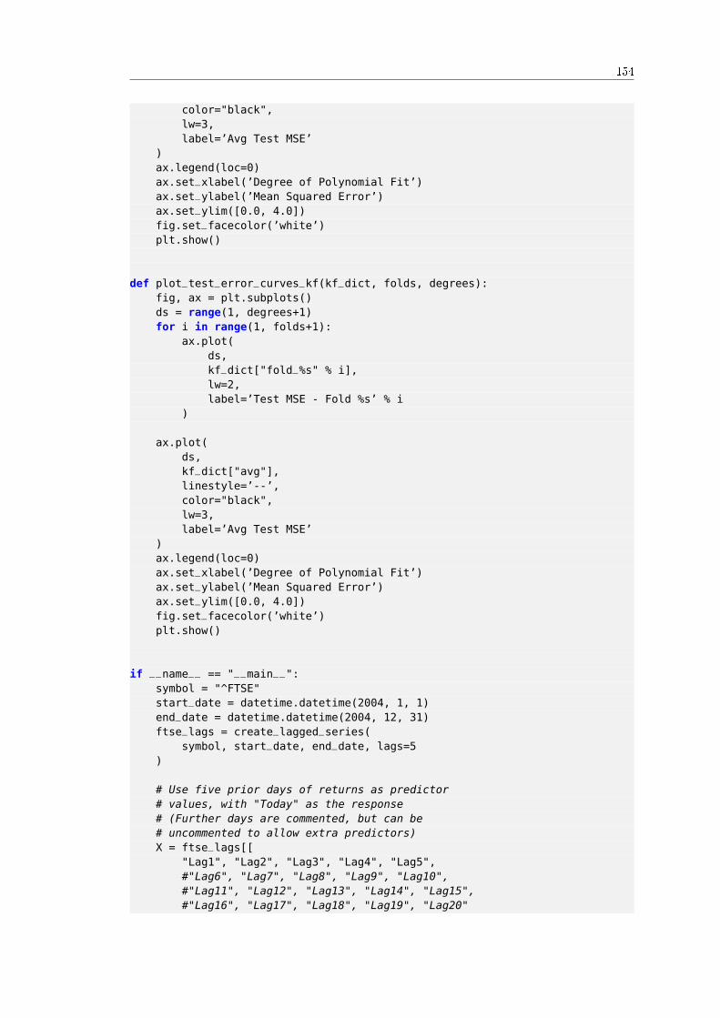
154

color="black",lw=3,label=’Avg Test MSE’

)ax.legend(loc=0)ax.set_xlabel(’Degree of Polynomial Fit’)ax.set_ylabel(’Mean Squared Error’)ax.set_ylim([0.0, 4.0])fig.set_facecolor(’white’)plt.show()

def plot_test_error_curves_kf(kf_dict, folds, degrees):fig, ax = plt.subplots()ds = range(1, degrees+1)for i in range(1, folds+1):

ax.plot(ds,kf_dict["fold_%s" % i],lw=2,label=’Test MSE - Fold %s’ % i

)

ax.plot(ds,kf_dict["avg"],linestyle=’--’,color="black",lw=3,label=’Avg Test MSE’

)ax.legend(loc=0)ax.set_xlabel(’Degree of Polynomial Fit’)ax.set_ylabel(’Mean Squared Error’)ax.set_ylim([0.0, 4.0])fig.set_facecolor(’white’)plt.show()

if __name__ == "__main__":symbol = "^FTSE"start_date = datetime.datetime(2004, 1, 1)end_date = datetime.datetime(2004, 12, 31)ftse_lags = create_lagged_series(

symbol, start_date, end_date, lags=5)

# Use five prior days of returns as predictor# values, with "Today" as the response# (Further days are commented, but can be# uncommented to allow extra predictors)X = ftse_lags[[

"Lag1", "Lag2", "Lag3", "Lag4", "Lag5",#"Lag6", "Lag7", "Lag8", "Lag9", "Lag10",#"Lag11", "Lag12", "Lag13", "Lag14", "Lag15",#"Lag16", "Lag17", "Lag18", "Lag19", "Lag20"

155

]]y = ftse_lags["Today"]degrees = 3

# Plot the test error curves for validation setrandom_seeds = 10sample_dict_val = validation_set_poly(

random_seeds, degrees, X, y)plot_test_error_curves_vs(

sample_dict_val, random_seeds, degrees)

# Plot the test error curves for k-fold CV setfolds = 10kf_dict = k_fold_cross_val_poly(

folds, degrees, X, y)plot_test_error_curves_kf(

kf_dict, folds, degrees)

156

Chapter 13

Kernel Methods and SVMs

13.1 Support Vector Machines

In this section we are going to discuss an extremely powerful machine learning technique knownas the Support Vector Machine (SVM). It is one of the best "out of the box" supervisedclassi�cation techniques. It is an important tool for both the quantitative trading researcher anddata scientist.

This section will cover the theory of maximal margin classi�ers, support vector clas-si�ers and support vector machines. We will be making use of Scikit-Learn to demonstratesome examples of the aforementioned theoretical techniques on actual data.

13.1.1 Motivation for Support Vector Machines

The problem to be solved in this section is one of supervised binary classi�cation. Thatis, we wish to categorise new unseen objects into two separate groups based on their propertiesand a set of known examples that are already categorised. A good example of such a systemis classifying a set of new documents into positive or negative sentiment groups, based on otherdocuments which have already been classi�ed as positive or negative. Similarly, we could classifynew emails into spam or non-spam, based on a large corpus of documents that have already beenmarked as spam or non-spam by humans. SVMs are highly applicable to such situations.

A Support Vector Machine models the situation by creating a feature space, which is a �nite-dimensional vector space, each dimension of which represents a "feature" of a particular object.In the context of spam or document classi�cation, each "feature" is the prevalence or importanceof a particular word.

The goal of the SVM is to train a model that assigns new unseen objects into a particularcategory. It achieves this by creating a linear partition of the feature space into two subspaces.Based on the features in the new unseen objects (e.g. documents/emails), it places an object"above" or "below" the separation plane, leading to a categorisation (e.g. spam or non-spam).This makes it an example of a non-probabilistic linear classi�er. It is non-probabilistic becausethe features in the new objects fully determine its location in feature space and there is nostochastic element involved.

However, much of the bene�t of SVMs comes from the fact that they are not restricted tobeing linear classi�ers. Utilising a technique known as the kernel trick they can become muchmore �exible by introducing various types of non-linear decision boundaries.

Formally, in mathematical language, SVMs construct linear separating hyperplanes in large�nite-dimensional vector spaces. Data points are viewed as (~x, y) tuples, ~x = (x1, . . . , xp) wherethe xj are the feature values and y is the classi�cation (usually given as +1 or −1). Optimalclassi�cation occurs when such hyperplanes provide maximal distance to the nearest trainingdata points. Intuitively, this makes sense, as if the points are well separated, the classi�cationbetween two groups is much clearer.

However, if in a feature space some of the sets are not linearly separable (i.e. they over-lap!), then it is necessary to perform a transformation of the original feature space to a higher-

157

158

dimensional space, in which the separation between the groups is clear, or at least clearer.However, this has the consequence of making the separation boundary in the original spacepotentially non-linear.

In this section we will proceed by considering the advantages and disadvantages of SVMs asa classi�cation technique. We will then de�ne the concept of an optimal linear separatinghyperplane, which motivates a simple type of linear classi�er known as a maximal margin clas-si�er (MMC). Subsequently we will show that maximal margin classi�ers are not often applicableto many "real world" situations and need modi�cation in the form of a support vector classi�er(SVC). We will then relax the restriction of linearity and consider non-linear classi�ers, namelysupport vector machines, which use kernel functions to improve computational e�ciency.

13.1.2 Advantages and Disadvantages of SVMs

As a classi�cation technique the SVM has many advantages, some of which are due to its com-putational e�ciency on large datasets. The Scikit-Learn team have summarised the main ad-vantages and disadvantages[4] but I have repeated and elaborated on them for completeness:

Advantages

� High-Dimensionality - The SVM is an e�ective tool in high-dimensional spaces, whichis particularly applicable to document classi�cation and sentiment analysis where the di-mensionality can be extremely large (≥ 106).

� Memory E�ciency - Since only a subset of the training points are used in the actualdecision process of assigning new members, only these points need to be stored in memory(and calculated upon) when making decisions.

� Versatility - Class separation is often highly non-linear. The ability to apply new kernelsallows substantial �exibility for the decision boundaries, leading to greater classi�cationperformance.

Disadvantages

� p > n - In situations where the number of features for each object (p) exceeds the number oftraining data samples (n), SVMs can perform poorly. This can be seen intuitively, as if thehigh-dimensional feature space is much larger than the number of samples, then there areless e�ective support vectors on which to support the optimal linear hyperplanes, leadingto poorer classi�cation performance as new unseen samples are added.

� Non-Probabilistic - Since the classi�er works by placing objects above and below aclassifying hyperplane, there is no direct probabilistic interpretation for group membership.However, one potential metric to determine "e�ectiveness" of the classi�cation is how farfrom the decision boundary the new point is.

Now that we've outlined the advantages and disadvantages we're going to discuss the geo-metric objects and mathematical entities that will ultimately allow us to de�ne the SVMs andhow they work.

There are some fantastic references (both links and textbooks) that derive much of the math-ematical detail of how SVMs function. In the following derivation I didn't want to "reinvent thewheel" too much, especially with regards notation and pedagogy, so I've formulated the followingtreatment based on the references provided, making strong use of James et al[32], Hastie et al[27]and the Wikibooks article on SVMs[5]. As this is a textbook on trading strategies, I have madechanges to the notation where appropriate and have adjusted the narrative to suit individualsinterested in quantitative trading.

159

13.1.3 Linear Separating Hyperplanes

The linear separating hyperplane is the key geometric entity that is at the heart of the SVM.Informally, if we have a high-dimensional feature space, then the linear hyperplane is an objectone dimension lower than this space that divides the feature space into two regions.

This linear separating plane need not pass through the origin of our feature space, i.e. it doesnot need to include the zero vector as an entity within the plane. Such hyperplanes are knownas a�ne.

If we consider a real-valued p-dimensional feature space, known mathematically as Rp, thenour linear separating hyperplane is an a�ne p− 1 dimensional space embedded within it.

For the case of p = 2 this hyperplane is simply a one-dimensional straight line, which livesin the larger two-dimensional plane, whereas for p = 3 the hyerplane is a two-dimensional planethat lives in the larger three-dimensional feature space (see Figure 13.1):

Figure 13.1: One- and two-dimensional hyperplanes

If we consider an element of our p-dimensional feature space, i.e. ~x = (x1, ..., xp) ∈ Rp, thenwe can mathematically de�ne an a�ne hyperplane by the following equation:

b0 + b1x1 + ...+ bpxp = 0 (13.1)

b0 6= 0 gives us an a�ne plane (i.e. it does not pass through the origin). We can use a moresuccinct notation for this equation by introducing the summation sign:

b0 +

p∑j=1

bjxj = 0 (13.2)

Notice however that this is nothing more than a multi-dimensional dot product (or, moregenerally, an inner product), and as such can be written even more succinctly as:

~b · ~x+ b0 = 0 (13.3)

If an element ~x ∈ Rp satis�es this relation then it lives on the p− 1-dimensional hyperplane.This hyperplane splits the p-dimensional feature space into two classi�cation regions (see Figure13.2):

Elements ~x above the plane satisfy:

~b · ~x+ b0 > 0 (13.4)

While those below it satisfy:

160

Figure 13.2: Separation of p-dimensional space by a hyperplane

~b · ~x+ b0 < 0 (13.5)

The key point here is that it is possible for us to determine which side of the plane any element~x will fall on by calculating the sign (i.e. whether it is positive or negative) of the expression~b · ~x+ b0. This concept will form the basis of a supervised classi�cation technique.

13.1.4 Classi�cation

Continuing with our example of email spam �ltering, we can think of our classi�cation problem(say) as being provided with a thousand emails (n = 1000), each of which is marked spam (+1)or non-spam (−1). In addition, each email has an associated set of keywords (i.e. separating thewords on spacing) that provide features. Hence if we take the set of all possible keywords fromall of the emails (and remove duplicates), we will be left with p keywords in total.

If we translate this into a mathematical problem, the standard setup for a supervised classi�-cation procedure is to consider a set of n training observations, ~xi, each of which is a p-dimensionalvector of features. Each training observation has an associated class label, yi ∈ {−1, 1}. Hencewe can think of n pairs of training observations (~xi, yi) representing the features and class labels(keyword lists and spam/non-spam). In addition to the training observations we can provide testobservations, ~x∗ = (x∗1, ..., x

∗p) that are later used to test the performance of the classi�ers. In

our spam example, these test observations would be new emails that have not yet been seen.Our goal is to develop a classi�er based on provided training observations that will correctly

classify subsequent test observations using only their feature values. This translates into beingable to classify an email as spam or non-spam solely based on the keywords contained within it.

We will initially suppose that it is possible, via a means yet to be determined, to constructa hyperplane that separates training data perfectly according to their class labels (see Figure13.3). This would mean cleanly separating spam emails from non-spam emails solely by usingspeci�c keywords. The following diagram is only showing p = 2, while for keyword lists we mayhave p > 106. Hence Figures 13.3 are only representative of the problem.

This translates into a mathematical separating property of:

~b · ~xi + b0 > 0, if yi = 1 (13.6)

and

161

Figure 13.3: Multiple separating hyperplanes; Perfect separation of class data

~b · ~xi + b0 < 0, if yi = −1 (13.7)

This basically states that if each training observation is above or below the separating hy-perplane, according to the geometric equation which de�nes the plane, then its associated classlabel will be +1 or −1. Thus we have developed a simple classi�cation process. We assign a testobservation to a class depending upon which side of the hyperplane it is located on.

This can be formalised by considering the following function f(~x), with a test observation~x∗ = (x∗1, ..., x

∗p):

f(~x∗) = ~b · ~x∗ + b0 (13.8)

If f(~x∗) > 0 then y∗ = +1, whereas if f(~x∗) < 0 then y∗ = −1.

However, this tells us nothing about how we go about �nding the bj components of ~b, as wellas b0, which are crucial in helping us determine the equation of the hyperplane separating thetwo regions. The next section discusses an approach for carrying this out, as well as introducingthe concept of the maximal margin hyperplane and a classi�er built on it, known as themaximal margin classi�er.

13.1.5 Deriving the Classi�er

At this stage it is worth pointing out that separating hyperplanes are not unique since it ispossible to slightly translate or rotate such a plane without touching any training observations(see Figures 13.3).

So, not only do we need to know how to construct such a plane, but we also need to determinethe most optimal plane. This motivates the concept of the maximal margin hyperplane(MMH), which is the separating hyperplane that is farthest from any training observations andis thus "optimal".

How do we �nd the maximal margin hyperplane? Firstly, we compute the perpendiculardistance from each training observation ~xi for a given separating hyperplane. The smallestperpendicular distance to a training observation from the hyperplane is known as the margin.The MMH is the separating hyperplane where the margin is the largest. This guarantees that itis the farthest minimum distance to a training observation.

The classi�cation procedure is then just simply a case of determining which side a test ob-servation falls on. This can be carried out using the above formula for f(~x∗). Such a classi�er isknown as a maximimal margin classi�er (MMC). Note however that �nding the particularvalues that lead to the MMH is purely based on the training observations. That is, we still needto be aware of how the MMC performs on the test observations. We are implicitly making the

162

assumption that a large margin in the training observations will provide a large margin on thetest observations, but this may not be the case.

As always, we must be careful to avoid over�tting when the number of feature dimensionsis large (e.g. in Natural Language Processing applications such as email spam classi�cation).Over�tting here means that the MMH is a very good �t for the training data but can performquite poorly when exposed to testing data. I discussed this issue in depth in the previous chapter,under the Bias-Variance Tradeo� section.

To reiterate, our goal now becomes �nding an algorithm that can produce the bj values,which will �x the geometry of the hyperplane and hence allow determination of f(~x∗) for anytest observation.

If we consider Figure 13.4, we can see that the MMH is the mid-line of the widest "block"that we can insert between the two classes such that they are perfectly separated.

Figure 13.4: Maximal margin hyperplane with support vectors (A, B and C)

One of the key features of the MMC (and subsequently SVC and SVM) is that the locationof the MMH only depends on the support vectors, which are the training observations thatlie directly on the margin (but not hyperplane) boundary (see points A, B and C in Figure13.4). This means that the location of the MMH is NOT dependent upon any other trainingobservations.

Thus it can be immediately seen that a potential drawback of the MMC is that its MMH (andthus its classi�cation performance) can be extremely sensitive to the support vector locations.However, it is also partially this feature that makes the SVM an attractive computational tool,as we only need to store the support vectors in memory once it has been "trained" (i.e. the bjvalues are �xed).

13.1.6 Constructing the Maximal Margin Classi�er

I feel it is instructive to fully outline the optimisation problem that needs to be solved in orderto create the MMH (and thus the MMC itself). While I will outline the constraints of theoptimisation problem, the algorithmic solution to this problem is beyond the scope of the book.Thankfully these optimisation routines are implemented in scikit-learn (actually, via the LIBSVMlibrary[16]). If you wish to read more about the solution to these algorithmic problems, take alook at Hastie et al (2009)[27] and the Scikit-Learn page on Support Vector Machines[4].

The procedure for determining a maximal margin hyperplane for a maximal margin classi�eris as follows. Given n training observations ~x1, ..., ~xn ∈ Rp and n class labels y1, ..., yn ∈ {−1, 1},the MMH is the solution to the following optimisation procedure:

Maximise M ∈ R, by varying b1, ..., bp such that:

163

p∑j=1

b2j = 1 (13.9)

and

yi

(~b · ~x+ b0

)≥M, ∀i = 1, ..., n (13.10)

Despite the complex looking constraints, they actually state that each observation must beon the correct side of the hyperplane and at least a distance M from it. Since the goal of theprocedure is to maximise M , this is precisely the condition we need to create the MMC!

Clearly, the case of perfect separability is an ideal one. Most "real world" datasets will nothave such perfect separability via a linear hyperplane (see Figure 13.5). However, if there is noseparability then we are unable to construct a MMC by the optimisation procedure above. So,how do we create a form of separating hyperplane?

Figure 13.5: No possibility of a true separating hyperplane

Essentially we have to relax the requirement that a separating hyperplane will perfectlyseparate every training observation on the correct side of the line (i.e. guarantee that it isassociated with its true class label), using what is called a soft margin. This motivates theconcept of a support vector classi�er (SVC).

13.1.7 Support Vector Classi�ers

As we alluded to above, one of the problems with MMC is that they can be extremely sensitiveto the addition of new training observations. Consider Figure 13.6. In the left panel it can beseen that there exists a MMH perfectly separating the two classes. However, in the right panelif we add one point to the +1 class we see that the location of the MMH changes substantially.Hence in this situation the MMH has clearly been over-�t :

As we mentioned above also, we could consider a classi�er based on a separating hyperplanethat doesn't perfectly separate the two classes, but does have a greater robustness to the additionof new invididual observations and has a better classi�cation onmost of the training observations.This comes at the expense of some misclassi�cation of a few training observations.

This is how a support vector classi�er or soft margin classi�er works. A SVC allows someobservations to be on the incorrect side of the margin (or hyperplane), hence it provides a "soft"separation. Figure 13.7 demonstrate observations being on the wrong side of the margin and thewrong side of the hyperplane respectively:

164

Figure 13.6: Addition of a single point dramatically changes the MMH line

Figure 13.7: Observations on the wrong side of the margin and hyperplane, respectively

As before, an observation is classi�ed depending upon which side of the separating hyperplaneit lies on, but some points may be misclassi�ed.

It is instructive to see how the optimisation procedure di�ers from that described above forthe MMC. We need to introduce new parameters, namely n εi values (known as the slack values)and a parameter C, known as the budget. We wish to maximise M , across b1, ..., bp, ε1, .., εn suchthat:

p∑j=1

b2j = 1 (13.11)

and

yi

(~b · ~x+ b0

)≥M(1− εi), ∀i = 1, ..., n (13.12)

and

εi ≥ 0,

n∑i=1

εi ≤ C (13.13)

Where C, the budget, is a non-negative "tuning" parameter. M still represents the marginand the slack variables εi allow the individual observations to be on the wrong side of the marginor hyperplane.

165

In essence the εi tell us where the ith observation is located relative to the margin andhyperplane. For εi = 0 it states that the xi training observation is on the correct side of themargin. For εi > 0 we have that xi is on the wrong side of the margin, while for εi > 1 we havethat xi is on the wrong side of the hyperplane.

C collectively controls how much the individual εi can be modi�ed to violate the margin.C = 0 implies that εi = 0,∀i and thus no violation of the margin is possible, in which case (forseparable classes) we have the MMC situation.

For C > 0 it means that no more than C observations can violate the hyperplane. As Cincreases the margin will widen. See Figure 13.8 for two di�ering values of C:

Figure 13.8: Di�erent values of the tuning parameter C

How do we choose C in practice? Generally this is done via cross-validation. In essence C isthe parameter that governs the bias-variance trade-o� for the SVC. A small value of C means alow bias, high variance situation. A large value of C means a high bias, low variance situation.

As before, to classify a new test observation x∗ we simply calculate the sign of f(~x∗) =~b · ~x∗ + b0.

This is all well and good for classes that are linearly (or nearly linearly) separated. However,what about separation boundaries that are non-linear? How do we deal with those situations?This is where we can extend the concept of support vector classi�ers to support vector machines.

13.1.8 Support Vector Machines

The motivation behind the extension of a SVC is to allow non-linear decision boundaries. This isthe domain of the Support Vector Machine (SVM). Consider the following Figure 13.9. In sucha situation a purely linear SVC will have extremely poor performance, simply because the datahas no clear linear separation:

Hence SVCs can be useless in highly non-linear class boundary problems.In order to motivate how an SVM works, we can consider a standard "trick" in linear re-

gression, when considering non-linear situations. In particular a set of p features x1, ..., xp canbe transformed, say, into a set of 2p features x1, x

21, ..., xp, x

2p. This allows us to apply a linear

technique to a set of non-linear features.While the decision boundary is linear in the new 2p-dimensional feature space it is non-linear

in the original p-dimensional space. We end up with a decision boundary given by q(~x) = 0 whereq is a quadratic polynomial function of the original features and hence is a non-linear solution.

This is clearly not restricted to quadratic polynomials. Higher dimensional polynomials,interaction terms and other functional forms, could all be considered. Although the drawback isthat it dramatically increases the dimension of the feature space to the point that some algorithmscan become untractable.

The major advantage of SVMs is that they allow a non-linear enlargening of the feature space,while still retaining a signi�cant computational e�ciency, using a process known as the "kernel

166

Figure 13.9: No clear linear separation between classes and thus poor SVC performance

trick", which will be outlined below shortly.So what are SVMs? In essence they are an extension of SVCs that results from enlargening

the feature space through the use of functions known as kernels. In order to understand kernels,we need to brie�y discuss some aspects of the solution to the SVC optimisation problem outlinedabove.

While calculating the solution to the SVC optimisation problem, the algorithm only needsto make use of inner products between the observations and not the observations themselves.Recall that an inner product is de�ned for two p-dimensional vectors u, v as:

〈~u,~v〉 =

p∑j=1

ujvj (13.14)

Hence for two observations an inner product is de�ned as:

〈~xi, ~xk〉 =

p∑j=1

xijxkj (13.15)

While we won't dwell on the details (since they are beyond the scope of this book), it ispossible to show that a linear support vector classi�er for a particular observation ~x can berepresented as a linear combination of inner products:

f(~x) = b0 +

n∑i=1

αi〈~x, ~xi〉 (13.16)

With n ai coe�cients, one for each of the training observations.To estimate the b0 and ai coe�cients we only need to calculate

(n2

)= n(n − 1)/2 inner

products between all pairs of training observations. In fact, we ONLY need to calculate theinner products for the subset of training observations that represent the support vectors. I willcall this subset S . This means that:

ai = 0 if ~xi /∈ S (13.17)

Hence we can rewrite the representation formula as:

f(x) = b0 +∑i∈S

ai〈~x, ~xi〉 (13.18)

167

This turns out to be a major advantage for computational e�ciency.

This now motivates the extension to SVMs. If we consider the inner product 〈~xi, ~xk〉 andreplace it with a more general inner product "kernel" function K = K(~xi, ~xk), we can modifythe SVC representation to use non-linear kernel functions and thus modify how we calculate"similarity" between two observations. For instance, to recover the SVC we just take K to be asfollows:

K(~xi, ~xk) =

p∑j=1

xijxkj (13.19)

Since this kernel is linear in its features the SVC is known as the linear SVC. We can alsoconsider polynomial kernels, of degree d:

K(~xi, ~xk) = (1 +

p∑j=1

xijxkj)d (13.20)

This provides a signi�cantly more �exible decision boundary and essentially amounts to �ttinga SVC in a higher-dimensional feature space involving d-degree polynomials of the features (seeFigure 13.10).

Figure 13.10: A d-degree polynomial kernel; A radial kernel

Hence, the de�nition of a support vector machine is a support vector classi�er with a non-linear kernel function.

We can also consider the popular radial kernel (see Figure 13.10):

K(~xi, ~xk) = exp

−γ p∑j=1

(xij − xkj)2

, γ > 0 (13.21)

So how do radial kernels work? They clearly di�er from polynomial kernels. Essentially if ourtest observation ~x∗ is far from a training observation ~xi in standard Euclidean distance then thesum

∑pj=1(x∗j − xij)2 will be large and thus K(~x∗, ~xi) will be very small. Hence this particular

training observation ~xi will have almost no e�ect on where the test observation ~x∗ is placed, viaf(~x∗).

Thus the radial kernel has extremely localised behaviour and only nearby training observa-tions to ~x∗ will have an impact on its class label.

168

13.2 Document Classi�cation using Support Vector Machines

In this section we will apply Support Vector Machines to the domain of natural language process-ing (NLP) for the purposes of sentiment analysis and ultimately automated trade �lter or signalgeneration. Our approach will be to use Support Vector Machines to classify text documentsinto mutually exclusive groups. Note that this is a supervised learning technique. Later in thebook we will look at unsupervised techniques for similar tasks.

13.2.1 Overview

There are a signi�cant number of steps to carry out between viewing a text document on a website, say, and using its content as an input to an automated trading strategy to generate trade�lters or signals. In particular, the following steps must be carried out:

� Automate the download of multiple, continually generated articles from external sourcesat a potentially high throughput

� Parse these documents for the relevant sections of text/information that require analysis,even if the format di�ers between documents

� Convert arbitrarily long passages of text (over many possible languages) into a consistentdata structure that can be understood by a classi�cation system

� Determine a set of groups (or labels) that each document will be a member of. Examplesinclude "positive" and "negative" or "bullish" and "bearish"

� Create a "training corpus" of documents that have known labels associated with them. Forinstance, a thousand �nancial articles may need tagging with the "bullish" or "bearish"labels

� Train the classi�er(s) on this corpus by means of a software library such as Python's scikit-learn (which we will be using below)

� Use the classi�er to label new documents, in an automated, ongoing manner.

� Assess the "classi�cation rate" and other associated performance metrics of the classi�er

� Integrate the classi�er into an automated trading system (such as QSTrader), either bymeans of �ltering other trade signals or generating new ones.

� Continually monitor the system and adjust it as necessary, its performance begins to de-grade

In this particular section we will avoid discussion of how to download multiple articles fromexternal sources and make use of a given dataset that already comes with its own provided labels.This will allow us to concentrate on the implementation of the "classi�cation pipeline", ratherthan spend a substantial amount of time obtaining and tagging documents.

While beyond the scope of this section, it is possible to make use of Python libraries, suchas ScraPy and BeautifulSoup, to automatically obtain many web-based articles and e�ectivelyextract their text-based data from the HTML making up the page data.

In later chapters of the book we will discuss how to integrate such a classi�er into a production-ready algorithmic trading system.

Hence, under the assumption that we have a document corpus that is pre-labelled (the processof which will be outlined below), we will begin by taking the training corpus and incorporating itinto a Python data structure that is suitable for pre-processing and consumption via the classi�er.

169

13.2.2 Supervised Document Classi�cation

Consider a set of text documents. Each document has an associated set of words, which we willcall "features". Each of these documents might be associated with a class label that describeswhat the article is about.

For instance, a set of articles from a website discussing pets might have articles that areprimarily about dogs, cats or hamsters (say). Certain words, such as "cage" (hamster), "leash"(dog) or "milk" (cat) might be more representative of certain pets than others. Supervisedclassi�ers are able to isolate certain words which are representative of certain labels (animals)by "learning" from a set of "training" articles, which are already pre-labelled, often in a manualfashion, by a human.

Mathematically, each of the j articles about pets within a training corpus have an associatedfeature vector Xj , with components of this vector representing "strength" of words (we willde�ne "strength" below). Each article also has an associated class label, yj , which in this casewould be the name of the pet most associated with the article.

The "supervision" of the training procedure occurs when a model is trained or �t to thisparticular data. This means that the classi�er is fed feature vector-class label pairs and it"learns" how representative features are for particular class labels. In the following example wewill use the SVM as our model and "train" it on a corpus (a collection of documents) which wewill have previously generated.

13.3 Preparing a Dataset for Classi�cation

A famous dataset that is used in machine learning classi�cation design is theReuters 21578 set,the details of which can be found here: http://www.daviddlewis.com/resources/testcollections/reuters21578/.It is one of the most widely used testing datasets for text classi�cation.

The set consists of a collection of news articles - a "corpus" - that are tagged with a selectionof topics and geographic locations. Thus it comes "ready made" to be used in classi�cation tests,since it is already pre-labelled.

We will now download, extract and prepare the dataset. The following instructions assumeyou have access to a command line interface, such as the Terminal that ships with Linux or MacOS X. If you are using Windows then you will need to download a Tar/GZIP extraction tool toget hold of the data, such as 7-Zip (http://www.7-zip.org/).

The Reuters 21578 dataset can be found at http://kdd.ics.uci.edu/databases/reuters21578/reuters21578.tar.gzas a compressed tar GZIP �le. The �rst task is to create a new working directory and downloadthe �le into it. Please modify the directory name below as you see �t:

cd ~mkdir -p quantstart/classification/datacd quantstart/classification/datawget http://kdd.ics.uci.edu/databases/reuters21578/reuters21578.tar.gz

On Windows you will need to use the respective command line syntax to create the directories,or use Windows Explorer, and use a web browser to download the data.

We can then unzip and untar the �le:

tar -zxvf reuters21578.tar.gz

On Windows you can use 7-Zip for this procedure.If we list the contents of the directory (ls -l) we can see the following (the permissions and

ownership details have been omitted for brevity):

... 186 Dec 4 1996 all-exchanges-strings.lc.txt

... 316 Dec 4 1996 all-orgs-strings.lc.txt

... 2474 Dec 4 1996 all-people-strings.lc.txt

... 1721 Dec 4 1996 all-places-strings.lc.txt

... 1005 Dec 4 1996 all-topics-strings.lc.txt

... 28194 Dec 4 1996 cat-descriptions_120396.txt

... 273802 Dec 10 1996 feldman-cia-worldfactbook-data.txt

170

... 1485 Jan 23 1997 lewis.dtd

... 36388 Sep 26 1997 README.txt

... 1324350 Dec 4 1996 reut2-000.sgm

... 1254440 Dec 4 1996 reut2-001.sgm

... 1217495 Dec 4 1996 reut2-002.sgm

... 1298721 Dec 4 1996 reut2-003.sgm

... 1321623 Dec 4 1996 reut2-004.sgm

... 1388644 Dec 4 1996 reut2-005.sgm

... 1254765 Dec 4 1996 reut2-006.sgm

... 1256772 Dec 4 1996 reut2-007.sgm

... 1410117 Dec 4 1996 reut2-008.sgm

... 1338903 Dec 4 1996 reut2-009.sgm

... 1371071 Dec 4 1996 reut2-010.sgm

... 1304117 Dec 4 1996 reut2-011.sgm

... 1323584 Dec 4 1996 reut2-012.sgm

... 1129687 Dec 4 1996 reut2-013.sgm

... 1128671 Dec 4 1996 reut2-014.sgm

... 1258665 Dec 4 1996 reut2-015.sgm

... 1316417 Dec 4 1996 reut2-016.sgm

... 1546911 Dec 4 1996 reut2-017.sgm

... 1258819 Dec 4 1996 reut2-018.sgm

... 1261780 Dec 4 1996 reut2-019.sgm

... 1049566 Dec 4 1996 reut2-020.sgm

... 621648 Dec 4 1996 reut2-021.sgm

... 8150596 Mar 12 1999 reuters21578.tar.gz

You will see that all the �les beginning with reut2- are .sgm, which means that they areStandard Generalized Markup Language (SGML)[1] �les. Unfortunately, Python deprecatedsgmllib from Python in 2.6 and fully removed it for Python 3. However, all is not lost becausewe can create our own SGML Parser class that overrides Python's built in HTMLParser[3].

Here is a single news item from one of the �les:

..

..<REUTERS TOPICS="YES" LEWISSPLIT="TRAIN"CGISPLIT="TRAINING-SET" OLDID="5544" NEWID="1"><DATE>26-FEB-1987 15:01:01.79</DATE><TOPICS><D>cocoa</D></TOPICS><PLACES><D>el-salvador</D><D>usa</D><D>uruguay</D></PLACES><PEOPLE></PEOPLE><ORGS></ORGS><EXCHANGES></EXCHANGES><COMPANIES></COMPANIES><UNKNOWN>&#5;&#5;&#5;C T&#22;&#22;&#1;f0704&#31;reuteu f BC-BAHIA-COCOA-REVIEW 02-26 0105</UNKNOWN><TEXT>&#2;<TITLE>BAHIA COCOA REVIEW</TITLE><DATELINE> SALVADOR, Feb 26 - </DATELINE><BODY>Showers continued throughout the week inthe Bahia cocoa zone, alleviating the drought since earlyJanuary and improving prospects for the coming temporao,although normal humidity levels have not been restored,Comissaria Smith said in its weekly review.

The dry period means the temporao will be late this year.Arrivals for the week ended February 22 were 155,221 bags

171

of 60 kilos making a cumulative total for the season of 5.93mln against 5.81 at the same stage last year. Again it seemsthat cocoa delivered earlier on consignment was included in thearrivals figures.

Comissaria Smith said there is still some doubt as to howmuch old crop cocoa is still available as harvesting haspractically come to an end. With total Bahia crop estimatesaround 6.4 mln bags and sales standing at almost 6.2 mln thereare a few hundred thousand bags still in the hands of farmers,middlemen, exporters and processors.

There are doubts as to how much of this cocoa would be fitfor export as shippers are now experiencing dificulties inobtaining +Bahia superior+ certificates.

In view of the lower quality over recent weeks farmers havesold a good part of their cocoa held on consignment.

Comissaria Smith said spot bean prices rose to 340 to 350cruzados per arroba of 15 kilos.

Bean shippers were reluctant to offer nearby shipment andonly limited sales were booked for March shipment at 1,750 to1,780 dlrs per tonne to ports to be named.

New crop sales were also light and all to open ports withJune/July going at 1,850 and 1,880 dlrs and at 35 and 45 dlrsunder New York july, Aug/Sept at 1,870, 1,875 and 1,880 dlrsper tonne FOB.

Routine sales of butter were made. March/April sold at4,340, 4,345 and 4,350 dlrs.

April/May butter went at 2.27 times New York May, June/Julyat 4,400 and 4,415 dlrs, Aug/Sept at 4,351 to 4,450 dlrs and at2.27 and 2.28 times New York Sept and Oct/Dec at 4,480 dlrs and2.27 times New York Dec, Comissaria Smith said.

Destinations were the U.S., Covertible currency areas,Uruguay and open ports.

Cake sales were registered at 785 to 995 dlrs forMarch/April, 785 dlrs for May, 753 dlrs for Aug and 0.39 timesNew York Dec for Oct/Dec.

Buyers were the U.S., Argentina, Uruguay and convertiblecurrency areas.

Liquor sales were limited with March/April selling at 2,325and 2,380 dlrs, June/July at 2,375 dlrs and at 1.25 times NewYork July, Aug/Sept at 2,400 dlrs and at 1.25 times New YorkSept and Oct/Dec at 1.25 times New York Dec, Comissaria Smithsaid.

Total Bahia sales are currently estimated at 6.13 mln bagsagainst the 1986/87 crop and 1.06 mln bags against the 1987/88crop.

Final figures for the period to February 28 are expected tobe published by the Brazilian Cocoa Trade Commission aftercarnival which ends midday on February 27.Reuter&#3;</BODY></TEXT></REUTERS>....

While it may be somewhat laborious to parse data in this manner, especially when comparedto the actual machine learning, I can fully reassure you that a large part of a data scientist'sor quant researcher's day is in actually getting the data into a format usable by the analysis

172

software! This particular activity is often jokingly referred to as "data wrangling". Hence I feelit is worth it for you to get some practice at it!

If we take a look at the topics �le, all-topics-strings.lc.txt, by typing

less all-topics-strings.lc.tx

we can see the following (I've removed most of it for brevity):

acqalumaustdlraustralbarleybfrbopcancarcasscastor-mealcastor-oilcastorseedcitruspulpcocoacoconutcoconut-oilcoffeecoppercopra-cakecorn......silversingdlrskrsorghumsoy-mealsoy-oilsoybeanstgstrategic-metalsugarsun-mealsun-oilsunseedtapiocateatintradetungtung-oilveg-oilwheatwoolwpiyenzinc

By calling:

cat all-topics-strings.lc.txt | wc -l

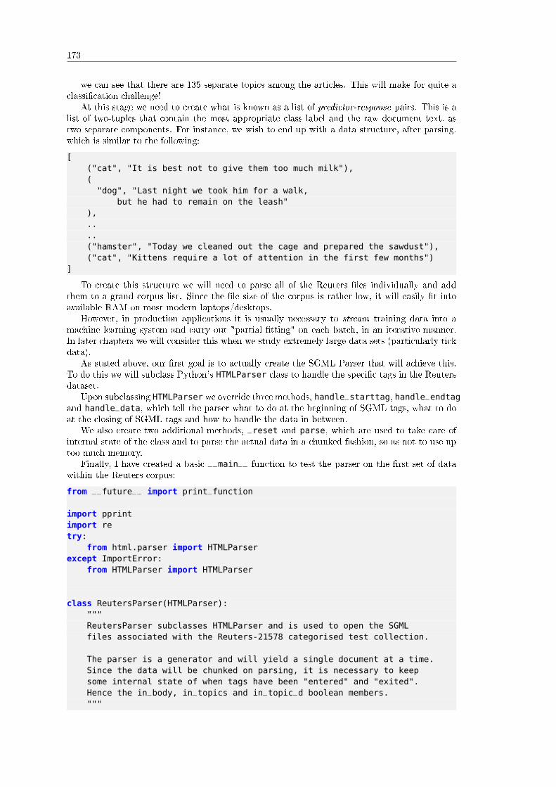
173

we can see that there are 135 separate topics among the articles. This will make for quite aclassi�cation challenge!

At this stage we need to create what is known as a list of predictor-response pairs. This is alist of two-tuples that contain the most appropriate class label and the raw document text, astwo separate components. For instance, we wish to end up with a data structure, after parsing,which is similar to the following:

[("cat", "It is best not to give them too much milk"),("dog", "Last night we took him for a walk,

but he had to remain on the leash"),....("hamster", "Today we cleaned out the cage and prepared the sawdust"),("cat", "Kittens require a lot of attention in the first few months")

]

To create this structure we will need to parse all of the Reuters �les individually and addthem to a grand corpus list. Since the �le size of the corpus is rather low, it will easily �t intoavailable RAM on most modern laptops/desktops.

However, in production applications it is usually necessary to stream training data into amachine learning system and carry out "partial �tting" on each batch, in an iterative manner.In later chapters we will consider this when we study extremely large data sets (particularly tickdata).

As stated above, our �rst goal is to actually create the SGML Parser that will achieve this.To do this we will subclass Python's HTMLParser class to handle the speci�c tags in the Reutersdataset.

Upon subclassing HTMLParser we override three methods, handle_starttag, handle_endtagand handle_data, which tell the parser what to do at the beginning of SGML tags, what to doat the closing of SGML tags and how to handle the data in between.

We also create two additional methods, _reset and parse, which are used to take care ofinternal state of the class and to parse the actual data in a chunked fashion, so as not to use uptoo much memory.

Finally, I have created a basic __main__ function to test the parser on the �rst set of datawithin the Reuters corpus:

from __future__ import print_function

import pprintimport retry:

from html.parser import HTMLParserexcept ImportError:

from HTMLParser import HTMLParser

class ReutersParser(HTMLParser):"""ReutersParser subclasses HTMLParser and is used to open the SGMLfiles associated with the Reuters-21578 categorised test collection.

The parser is a generator and will yield a single document at a time.Since the data will be chunked on parsing, it is necessary to keepsome internal state of when tags have been "entered" and "exited".Hence the in_body, in_topics and in_topic_d boolean members."""

174

def __init__(self, encoding=’latin-1’):"""Initialise the superclass (HTMLParser) and reset the parser.Sets the encoding of the SGML files by default to latin-1."""HTMLParser.__init__(self)self._reset()self.encoding = encoding

def _reset(self):"""This is called only on initialisation of the parser classand when a new topic-body tuple has been generated. Itresets all off the state so that a new tuple can be subsequentlygenerated."""self.in_body = Falseself.in_topics = Falseself.in_topic_d = Falseself.body = ""self.topics = []self.topic_d = ""

def parse(self, fd):"""parse accepts a file descriptor and loads the data in chunksin order to minimise memory usage. It then yields new documentsas they are parsed."""self.docs = []for chunk in fd:

self.feed(chunk.decode(self.encoding))for doc in self.docs:

yield docself.docs = []

self.close()

def handle_starttag(self, tag, attrs):"""This method is used to determine what to do when the parsercomes across a particular tag of type "tag". In this instancewe simply set the internal state booleans to True if that particulartag has been found."""if tag == "reuters":

passelif tag == "body":

self.in_body = Trueelif tag == "topics":

self.in_topics = Trueelif tag == "d":

self.in_topic_d = True

def handle_endtag(self, tag):"""This method is used to determine what to do when the parser

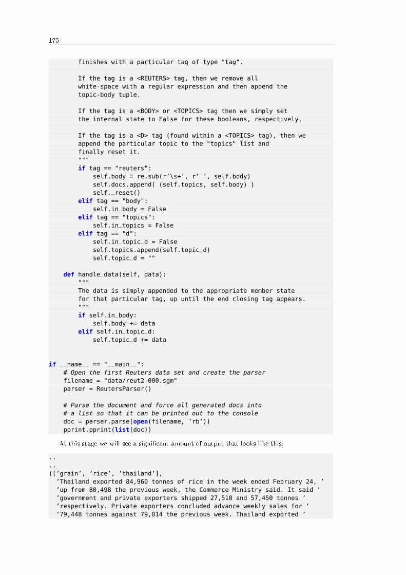
175

finishes with a particular tag of type "tag".

If the tag is a <REUTERS> tag, then we remove allwhite-space with a regular expression and then append thetopic-body tuple.

If the tag is a <BODY> or <TOPICS> tag then we simply setthe internal state to False for these booleans, respectively.

If the tag is a <D> tag (found within a <TOPICS> tag), then weappend the particular topic to the "topics" list andfinally reset it."""if tag == "reuters":

self.body = re.sub(r’\s+’, r’ ’, self.body)self.docs.append( (self.topics, self.body) )self._reset()

elif tag == "body":self.in_body = False

elif tag == "topics":self.in_topics = False

elif tag == "d":self.in_topic_d = Falseself.topics.append(self.topic_d)self.topic_d = ""

def handle_data(self, data):"""The data is simply appended to the appropriate member statefor that particular tag, up until the end closing tag appears."""if self.in_body:

self.body += dataelif self.in_topic_d:

self.topic_d += data

if __name__ == "__main__":# Open the first Reuters data set and create the parserfilename = "data/reut2-000.sgm"parser = ReutersParser()

# Parse the document and force all generated docs into# a list so that it can be printed out to the consoledoc = parser.parse(open(filename, ’rb’))pprint.pprint(list(doc))

At this stage we will see a signi�cant amount of output that looks like this:

..

..([’grain’, ’rice’, ’thailand’],’Thailand exported 84,960 tonnes of rice in the week ended February 24, ’’up from 80,498 the previous week, the Commerce Ministry said. It said ’’government and private exporters shipped 27,510 and 57,450 tonnes ’’respectively. Private exporters concluded advance weekly sales for ’’79,448 tonnes against 79,014 the previous week. Thailand exported ’

176

’689,038 tonnes of rice between the beginning of January and February 24, ’’up from 556,874 tonnes during the same period last year. It has ’’commitments to export another 658,999 tonnes this year. REUTER ’),([’soybean’, ’red-bean’, ’oilseed’, ’japan’],’The Tokyo Grain Exchange said it will raise the margin requirement on ’’the spot and nearby month for U.S. And Chinese soybeans and red beans, ’’effective March 2. Spot April U.S. Soybean contracts will increase to ’’90,000 yen per 15 tonne lot from 70,000 now. Other months will stay ’’unchanged at 70,000, except the new distant February requirement, which ’’will be set at 70,000 from March 2. Chinese spot March will be set at ’’110,000 yen per 15 tonne lot from 90,000. The exchange said it raised ’’spot March requirement to 130,000 yen on contracts outstanding at March ’’13. Chinese nearby April rises to 90,000 yen from 70,000. Other months ’’will remain unchanged at 70,000 yen except new distant August, which ’’will be set at 70,000 from March 2. The new margin for red bean spot ’’March rises to 150,000 yen per 2.4 tonne lot from 120,000 and to 190,000 ’’for outstanding contracts as of March 13. The nearby April requirement ’’for red beans will rise to 100,000 yen from 60,000, effective March 2. ’’The margin money for other red bean months will remain unchanged at ’’60,000 yen, except new distant August, for which the requirement will ’’also be set at 60,000 from March 2. REUTER ’),

..

..

In particular, note that instead of having a single topic label associated with a document,we have multiple topics. In order to increase the e�ectiveness of the classi�er, it is necessaryto assign only a single class label to each document. However, you'll also note that some ofthe labels are actually geographic location tags, such as "japan" or "thailand". Since we areconcerned solely with topics and not countries we want to remove these before we select ourtopic.

The particular method that we will use to carry this out is rather simple. We will strip outthe country names and then select the �rst remaining topic on the list. If there are no associatedtopics we will eliminate the article from our corpus. In the above output, this will reduce to adata structure that looks like:

..

..(’grain’,’Thailand exported 84,960 tonnes of rice in the week ended February 24, ’’up from 80,498 the previous week, the Commerce Ministry said. It said ’’government and private exporters shipped 27,510 and 57,450 tonnes ’’respectively. Private exporters concluded advance weekly sales for ’’79,448 tonnes against 79,014 the previous week. Thailand exported ’’689,038 tonnes of rice between the beginning of January and February 24, ’’up from 556,874 tonnes during the same period last year. It has ’’commitments to export another 658,999 tonnes this year. REUTER ’),(’soybean’,’The Tokyo Grain Exchange said it will raise the margin requirement on ’’the spot and nearby month for U.S. And Chinese soybeans and red beans, ’’effective March 2. Spot April U.S. Soybean contracts will increase to ’’90,000 yen per 15 tonne lot from 70,000 now. Other months will stay ’’unchanged at 70,000, except the new distant February requirement, which ’’will be set at 70,000 from March 2. Chinese spot March will be set at ’’110,000 yen per 15 tonne lot from 90,000. The exchange said it raised ’’spot March requirement to 130,000 yen on contracts outstanding at March ’’13. Chinese nearby April rises to 90,000 yen from 70,000. Other months ’’will remain unchanged at 70,000 yen except new distant August, which ’

177

’will be set at 70,000 from March 2. The new margin for red bean spot ’’March rises to 150,000 yen per 2.4 tonne lot from 120,000 and to 190,000 ’’for outstanding contracts as of March 13. The nearby April requirement ’’for red beans will rise to 100,000 yen from 60,000, effective March 2. ’’The margin money for other red bean months will remain unchanged at ’’60,000 yen, except new distant August, for which the requirement will ’’also be set at 60,000 from March 2. REUTER ’),

..

..

To remove the geographic tags and select the primary topic tag we can add the followingcode:

..

..

def obtain_topic_tags():"""Open the topic list file and import all of the topic namestaking care to strip the trailing "\n" from each word."""topics = open(

"data/all-topics-strings.lc.txt", "r").readlines()topics = [t.strip() for t in topics]return topics

def filter_doc_list_through_topics(topics, docs):"""Reads all of the documents and creates a new list of two-tuplesthat contain a single feature entry and the body text, instead ofa list of topics. It removes all geographic features and onlyretains those documents which have at least one non-geographictopic."""ref_docs = []for d in docs:

if d[0] == [] or d[0] == "":continue

for t in d[0]:if t in topics:

d_tup = (t, d[1])ref_docs.append(d_tup)break

return ref_docs

if __name__ == "__main__":# Open the first Reuters data set and create the parserfilename = "data/reut2-000.sgm"parser = ReutersParser()

# Parse the document and force all generated docs into# a list so that it can be printed out to the consoledocs = list(parser.parse(open(filename, ’rb’)))

# Obtain the topic tags and filter docs through it

178

topics = obtain_topic_tags()ref_docs = filter_doc_list_through_topics(topics, docs)pprint.pprint(ref_docs)

The output from this is as follows:

..

..(’acq’,’Security Pacific Corp said it completed its planned merger with Diablo ’’Bank following the approval of the comptroller of the currency. Security ’’Pacific announced its intention to merge with Diablo Bank, headquartered ’’in Danville, Calif., in September 1986 as part of its plan to expand its ’’retail network in Northern California. Diablo has a bank offices in ’’Danville, San Ramon and Alamo, Calif., Security Pacific also said. ’’Reuter ’),(’earn’,’Shr six cts vs five cts Net 188,000 vs 130,000 Revs 12.2 mln vs 10.1 mln ’’Avg shrs 3,029,930 vs 2,764,544 12 mths Shr 81 cts vs 1.45 dlrs Net ’’2,463,000 vs 3,718,000 Revs 52.4 mln vs 47.5 mln Avg shrs 3,029,930 vs ’’2,566,680 NOTE: net for 1985 includes 500,000, or 20 cts per share, for ’’proceeds of a life insurance policy. includes tax benefit for prior qtr ’’of approximately 150,000 of which 140,000 relates to a lower effective ’’tax rate based on operating results for the year as a whole. Reuter ’),

..

..

We are now in a position to pre-process the data for input into the classi�er.

13.3.1 Vectorisation

At this stage we have a large collection of two-tuples, each containing a class label and raw bodytext from the articles. The obvious question to ask now is how do we convert the raw body textinto a data representation that can be used by a (numerical) classi�er?

The answer lies in a process known as vectorisation. Vectorisation allows widely-varyinglengths of raw text to be converted into a numerical format that can be processed by the classi�er.

It achieves this by creating tokens from a string. A token is an individual word (or group ofwords) extracted from a document, using whitespace or punctuation as separators. This can, ofcourse, include numbers from within the string as additional "words". Once this list of tokenshas been created they can be assigned an integer identi�er, which allows them to be listed.

Once the list of tokens have been generated, the number of tokens within a document arecounted. Finally, these tokens are normalised to de-emphasise tokens that appear frequentlywithin a document (such as "a", "the"). This process is known as the Bag Of Words.

The Bag Of Words representation allows a vector to be associated with each document,each component of which is real-valued (i.e. ∈ R) and represents the importance of tokens (i.e."words") appearing within that document.

Furthermore it means that once an entire corpus of documents has been iterated over (andthus all possible tokens have been assessed) the total number of separate tokens is known. Hencethe length of the token vector for any document of any length is also �xed and identical.

This means that the classi�er now has a set of features via the frequency of token occurance.In addition the document token-vector represents a sample for the classi�er.

In essence, the entire corpus can be represented as a large matrix, each row of which representsone of the documents and each column represents token occurance within that document. Thisis the process of vectorisation.

Note that vectorisation does not take into account the relative positioning of the words withinthe document, just the frequency of occurance. More sophisticated machine learning techniqueswill, however, use this information to enhance the classi�cation process.

179

13.3.2 Term-Frequency Inverse Document-Frequency

One of the major issues with vectorisation, via the Bag Of Words representation, is thatthere is a lot of "noise" in the form of stop words, such as "a", "the", "he", "she" etc. Thesewords provide little context to the document but their relatively high frequency will mean thatthey can mask words that do provide document context.

This motivates a transformation process, known as Term-Frequency Inverse Document-Frequency (TF-IDF). The TF-IDF value for a token increases proportionally to the frequencyof the word in the document but is normalised by the frequency of the word in the corpus. Thisessentially reduces importance for words that appear a lot generally, as opposed to appearing alot within a particular document.

This is precisely what we need as words such as "a", "the" will have extremely high occuranceswithin the entire corpus, but the word "cat" may only appear often in a particular document.This would mean that we are giving "cat" a relatively higher strength than "a" or "the", forthat document.

It isn't necessary dwell on the calculation of TF-IDF, but if you are interested then you canread the Wikipedia article[6] on the subject, which goes into more detail.

Hence we wish to combine the process of vectorisation with that of TF-IDF to produce anormalised matrix of document-token occurances. This will then be used to provide a list offeatures to the classi�er upon which to train.

Thankfully, the developers of the Python Scikit-Learn library realised that it would be anextremely common operation to vectorise and transform text �les in this manner and so includedthe TfidfVectorizer class.

We can use this class to take our list of two-tuples representing class labels and raw documenttext, to produce both a vector of class labels and a sparse matrix, which represents the TF-IDFand Vectorisation procedure applied to the raw text data.

Since Scikit-Learn classi�ers take two separate data structures for training, namely, y, thevector of class labels or "responses" associated with an ordered set of documents, and, X, thesparse TF-IDF matrix of raw document text, we modify our two-tuple list to create y and X.The code to create these objects is given below:

..from sklearn.feature_extraction.text import TfidfVectorizer....

def create_tfidf_training_data(docs):"""Creates a document corpus list (by stripping out theclass labels), then applies the TF-IDF transform to thislist.

The function returns both the class label vector (y) andthe corpus token/feature matrix (X)."""# Create the training data class labelsy = [d[0] for d in docs]

# Create the document corpus listcorpus = [d[1] for d in docs]

# Create the TF-IDF vectoriser and transform the corpusvectorizer = TfidfVectorizer(min_df=1)X = vectorizer.fit_transform(corpus)return X, y

180

if __name__ == "__main__":# Open the first Reuters data set and create the parserfilename = "data/reut2-000.sgm"parser = ReutersParser()

# Parse the document and force all generated docs into# a list so that it can be printed out to the consoledocs = list(parser.parse(open(filename, ’rb’)))

# Obtain the topic tags and filter docs through ittopics = obtain_topic_tags()ref_docs = filter_doc_list_through_topics(topics, docs)

# Vectorise and TF-IDF transform the corpusX, y = create_tfidf_training_data(ref_docs)

At this stage we now have two components to our training data. The �rst, X, is a matrixof document-token occurances. The second, y, is a vector (which matches the ordering of thematrix) that contains the correct class labels for each of the documents. This is all we need tobegin training and testing the Support Vector Machine.

13.4 Training the Support Vector Machine

In order to train the Support Vector Machine it is necessary to provide it with both a set offeatures (the X matrix) and a set of "supervised" training labels, in this case the y classes.However, we also need a means of evaluating the trained performance of the classi�er subsequentto its training phase. We discussed approaches for this in the previous chapter on cross-validation.

One question that arises here is what percentage to retain for training and what to use fortesting. Clearly the more that is retained for training, the "better" the classi�er will be becauseit will have seen more data. More training data means less testing data and as such will lead toa poorer estimate of its true classi�cation capability. In this section we will retain approximatelyabout 70-80% of the data for training and use the remainder for testing. A more sophisticatedapproach would be to use k-fold cross-validation.

Since the training-test split is such a common operation in machine learning, the developersof Scikit-Learn provided the train_test_split method to automatically create the split froma dataset provided (which we have already discussed in the previous chapter). Here is the codethat provides the split:

from sklearn.cross_validation import train_test_split....X_train, X_test, y_train, y_test = train_test_split(X, y, test_size=0.2, random_state=42

)

The test_size keyword argument controls the size of the testing set, in this case 20%. Therandom_state keyword argument controls the random seed for selecting the partition randomly.

The next step is to actually create the Support Vector Machine and train it. In this instancewe are going to use the SVC (Support Vector Classi�er) class from Scikit-Learn. We give it theparameters C = 1000000.0, γ = 0.0 and choose a radial kernel. To understand where theseparameters come from, please take a look at the previous section on Support Vector Machines

The following code imports the SVC class and then �ts it on the training data:

from sklearn.svm import SVC....def train_svm(X, y):

"""

181

Create and train the Support Vector Machine."""svm = SVC(C=1000000.0, gamma=0.0, kernel=’rbf’)svm.fit(X, y)return svm

if __name__ == "__main__":# Open the first Reuters data set and create the parserfilename = "data/reut2-000.sgm"parser = ReutersParser()

# Parse the document and force all generated docs into# a list so that it can be printed out to the consoledocs = list(parser.parse(open(filename, ’rb’)))

# Obtain the topic tags and filter docs through ittopics = obtain_topic_tags()ref_docs = filter_doc_list_through_topics(topics, docs)

# Vectorise and TF-IDF transform the corpusX, y = create_tfidf_training_data(ref_docs)

# Create the training-test split of the dataX_train, X_test, y_train, y_test = train_test_split(

X, y, test_size=0.2, random_state=42)

# Create and train the Support Vector Machinesvm = train_svm(X_train, y_train)

Now that the SVM has been trained we need to assess its performance on the testing data.

13.4.1 Performance Metrics

The two main performance metrics that we will consider for this supervised classifer are thehit-rate and the confusion matrix. The former is simply the ratio of correct assignments tototal assignments and is usually quoted as a percentage.

The confusion matrix goes into more detail and provides output on true-positives, true-negatives, false-positives and false-negatives. In a binary classi�cation system, with a "true"or "false" class labelling, these characterise the rate at which the classi�er correctly classi�esan entity as true or false when it is, respectively, true or false, and also incorrectly classi�es anentity as true or false when it is, respectively, false or true.

A confusion matrix need not be restricted to a binary classi�cation situation. For multipleclass groups (as in our situation with the Reuters dataset) we will have an N ×N matrix, whereN is the number of class labels (or document topics).

Scikit-Learn has functions for calculating both the hit-rate and the confusion matrix of asupervised classi�er. The former is a method on the classi�er itself called score. The lattermust be imported from the metrics library.

The �rst task is to create a predictions array from the X_test test-set. This will simplycontain the predicted class labels from the SVM via the retained 20% test set. This predictionarray is used to create the confusion matrix. Notice that the confusion_matrix function takesboth the pred predictions array and the y_test correct class labels to produce the matrix. Inaddition we create the hit-rate by providing score with both the X_test and y_test subsets ofthe dataset:

..

182

..from sklearn.metrics import confusion_matrix....

if __name__ == "__main__":

..

..

# Create and train the Support Vector Machinesvm = train_svm(X_train, y_train)

# Make an array of predictions on the test setpred = svm.predict(X_test)

# Output the hit-rate and the confusion matrix for each modelprint(svm.score(X_test, y_test))print(confusion_matrix(pred, y_test))

The output of the code is as follows:

0.660194174757[[21 0 0 0 2 3 0 0 0 1 0 0 0 0 1 1 1 0 0][ 0 0 0 0 0 0 0 0 0 0 0 0 0 0 0 0 0 0 0][ 0 0 1 0 0 0 0 0 0 0 0 0 0 0 0 0 0 0 0][ 0 0 0 1 0 0 0 0 0 0 0 0 0 0 0 0 0 0 0][ 0 0 0 0 4 0 0 0 0 0 0 0 0 0 0 0 0 0 0][ 0 1 0 0 1 26 0 0 0 1 0 1 0 1 0 0 0 0 0][ 0 0 0 0 0 0 2 0 0 0 0 0 0 0 0 0 0 0 1][ 0 0 0 0 0 0 0 1 0 0 0 0 0 0 0 0 0 0 0][ 0 0 0 0 0 0 0 0 0 0 0 0 0 0 0 0 0 0 0][ 0 0 0 0 1 0 0 0 0 3 0 0 0 0 0 0 0 0 0][ 3 0 0 1 2 2 3 0 1 1 6 0 1 0 0 0 2 3 0][ 0 0 0 0 0 0 0 0 0 0 0 0 0 0 0 0 0 0 0][ 0 0 0 0 0 0 0 0 0 0 0 0 0 0 0 0 0 0 0][ 0 0 0 0 0 0 0 0 0 0 0 0 0 1 0 0 0 0 0][ 0 0 0 0 0 0 0 0 0 0 0 0 0 0 1 0 0 0 0][ 0 0 0 0 0 0 0 0 0 0 0 0 0 0 0 1 0 0 0][ 0 0 0 0 0 0 0 0 0 0 0 0 0 0 0 0 0 0 0][ 0 0 0 0 0 0 0 0 0 0 0 0 0 0 0 0 0 0 0][ 0 0 0 0 0 0 0 0 0 0 0 0 0 0 0 0 0 0 0]]

Thus we have a 66% classi�cation hit rate, with a confusion matrix that has entries mainlyon the diagonal (i.e. the correct assignment of class label). Notice that since we are only using asingle �le from the Reuters set (number 000), we aren't going to see the entire set of class labelsand hence our confusion matrix is smaller in dimension than if we had used the full dataset.

In order to make use of the full dataset we can modify the __main__ function to load all 21Reuters �les and train the SVM on the full dataset. We can output the full hit-rate performance.I've neglected to include the confusion matrix output as it becomes large for the total numberof class labels within all documents. Note that this will take some time! On my system it takesabout 30-45 seconds to run.

if __name__ == "__main__":# Create the list of Reuters data and create the parserfiles = ["data/reut2-%03d.sgm" % r for r in range(0, 22)]parser = ReutersParser()

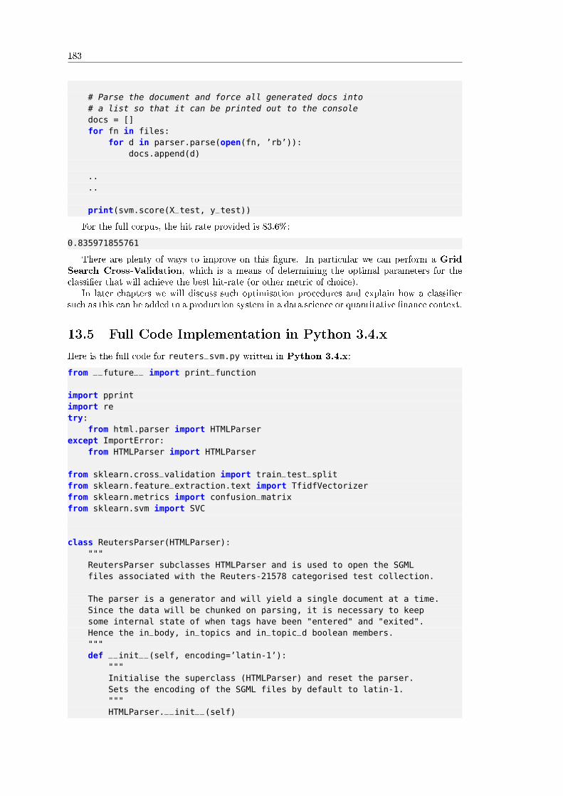
183

# Parse the document and force all generated docs into# a list so that it can be printed out to the consoledocs = []for fn in files:

for d in parser.parse(open(fn, ’rb’)):docs.append(d)

..

..

print(svm.score(X_test, y_test))

For the full corpus, the hit rate provided is 83.6%:

0.835971855761

There are plenty of ways to improve on this �gure. In particular we can perform a GridSearch Cross-Validation, which is a means of determining the optimal parameters for theclassi�er that will achieve the best hit-rate (or other metric of choice).

In later chapters we will discuss such optimisation procedures and explain how a classi�ersuch as this can be added to a production system in a data science or quantitative �nance context.

13.5 Full Code Implementation in Python 3.4.x

Here is the full code for reuters_svm.py written in Python 3.4.x:

from __future__ import print_function

import pprintimport retry:

from html.parser import HTMLParserexcept ImportError:

from HTMLParser import HTMLParser

from sklearn.cross_validation import train_test_splitfrom sklearn.feature_extraction.text import TfidfVectorizerfrom sklearn.metrics import confusion_matrixfrom sklearn.svm import SVC

class ReutersParser(HTMLParser):"""ReutersParser subclasses HTMLParser and is used to open the SGMLfiles associated with the Reuters-21578 categorised test collection.

The parser is a generator and will yield a single document at a time.Since the data will be chunked on parsing, it is necessary to keepsome internal state of when tags have been "entered" and "exited".Hence the in_body, in_topics and in_topic_d boolean members."""def __init__(self, encoding=’latin-1’):

"""Initialise the superclass (HTMLParser) and reset the parser.Sets the encoding of the SGML files by default to latin-1."""HTMLParser.__init__(self)

184

self._reset()self.encoding = encoding

def _reset(self):"""This is called only on initialisation of the parser classand when a new topic-body tuple has been generated. Itresets all off the state so that a new tuple can be subsequentlygenerated."""self.in_body = Falseself.in_topics = Falseself.in_topic_d = Falseself.body = ""self.topics = []self.topic_d = ""

def parse(self, fd):"""parse accepts a file descriptor and loads the data in chunksin order to minimise memory usage. It then yields new documentsas they are parsed."""self.docs = []for chunk in fd:

self.feed(chunk.decode(self.encoding))for doc in self.docs:

yield docself.docs = []

self.close()

def handle_starttag(self, tag, attrs):"""This method is used to determine what to do when the parsercomes across a particular tag of type "tag". In this instancewe simply set the internal state booleans to True if that particulartag has been found."""if tag == "reuters":

passelif tag == "body":

self.in_body = Trueelif tag == "topics":

self.in_topics = Trueelif tag == "d":

self.in_topic_d = True

def handle_endtag(self, tag):"""This method is used to determine what to do when the parserfinishes with a particular tag of type "tag".

If the tag is a <REUTERS> tag, then we remove allwhite-space with a regular expression and then append thetopic-body tuple.

185

If the tag is a <BODY> or <TOPICS> tag then we simply setthe internal state to False for these booleans, respectively.

If the tag is a <D> tag (found within a <TOPICS> tag), then weappend the particular topic to the "topics" list andfinally reset it."""if tag == "reuters":

self.body = re.sub(r’\s+’, r’ ’, self.body)self.docs.append( (self.topics, self.body) )self._reset()

elif tag == "body":self.in_body = False

elif tag == "topics":self.in_topics = False

elif tag == "d":self.in_topic_d = Falseself.topics.append(self.topic_d)self.topic_d = ""

def handle_data(self, data):"""The data is simply appended to the appropriate member statefor that particular tag, up until the end closing tag appears."""if self.in_body:

self.body += dataelif self.in_topic_d:

self.topic_d += data

def obtain_topic_tags():"""Open the topic list file and import all of the topic namestaking care to strip the trailing "\n" from each word."""topics = open(

"data/all-topics-strings.lc.txt", "r").readlines()topics = [t.strip() for t in topics]return topics

def filter_doc_list_through_topics(topics, docs):"""Reads all of the documents and creates a new list of two-tuplesthat contain a single feature entry and the body text, instead ofa list of topics. It removes all geographic features and onlyretains those documents which have at least one non-geographictopic."""ref_docs = []for d in docs:

if d[0] == [] or d[0] == "":continue

for t in d[0]:if t in topics:

186

d_tup = (t, d[1])ref_docs.append(d_tup)break

return ref_docs

def create_tfidf_training_data(docs):"""Creates a document corpus list (by stripping out theclass labels), then applies the TF-IDF transform to thislist.

The function returns both the class label vector (y) andthe corpus token/feature matrix (X)."""# Create the training data class labelsy = [d[0] for d in docs]

# Create the document corpus listcorpus = [d[1] for d in docs]

# Create the TF-IDF vectoriser and transform the corpusvectorizer = TfidfVectorizer(min_df=1)X = vectorizer.fit_transform(corpus)return X, y

def train_svm(X, y):"""Create and train the Support Vector Machine."""svm = SVC(C=1000000.0, gamma=0.0, kernel=’rbf’)svm.fit(X, y)return svm

if __name__ == "__main__":# Create the list of Reuters data and create the parserfiles = ["data/reut2-%03d.sgm" % r for r in range(0, 22)]parser = ReutersParser()

# Parse the document and force all generated docs into# a list so that it can be printed out to the consoledocs = []for fn in files:

for d in parser.parse(open(fn, ’rb’)):docs.append(d)

# Obtain the topic tags and filter docs through ittopics = obtain_topic_tags()ref_docs = filter_doc_list_through_topics(topics, docs)

# Vectorise and TF-IDF transform the corpusX, y = create_tfidf_training_data(ref_docs)

# Create the training-test split of the dataX_train, X_test, y_train, y_test = train_test_split(

X, y, test_size=0.2, random_state=42

187

)

# Create and train the Support Vector Machinesvm = train_svm(X_train, y_train)

# Make an array of predictions on the test setpred = svm.predict(X_test)

# Output the hit-rate and the confusion matrix for each modelprint(svm.score(X_test, y_test))print(confusion_matrix(pred, y_test))

13.5.1 Biblographic Notes

Originally, SVMs were invented by Vapnik[47], while the current standard "soft margin" approachis due to Cortes[17]. My treatment of the material follows, and is strongly in�uenced by, theexcellent statistical machine learning texts of James et al[32] and Hastie et al[27].

188

Part V

Quantitative Trading Strategies

189

Chapter 14

Introduction to QSTrader

In this chapter I want to brie�y introduce the QSTrader library, which will eventually be usedfor all of the trading strategies outlined in this book.

14.1 Backtesting vs Live Trading

One of the most important moments in the development of a quantitative trading strategy occurswhen a backtested strategy is �nally set to trade live.

Unfortunately, the performance of a deployed strategy is often signi�cantly worse than thatof a backtested system. There are many reasons for this:

� Transaction costs - These includes spread, fees, slippage and market impact.

� Latency to liquidity provider - This is the time taken between issuing an order to abrokerage and the brokerage executing it.

� Market regime change - A strategy or portfolio might have behaved well in previousmarket conditions, but fundamental changes to the market (such as a new regulatoryenvironment) reduce the performance of the strategy.

� Alpha decay - This describes the concept of the strategy being replicated by multipleusers over time, thus "arbitraging away" the edge.

The most common reason for signi�cant underperformance when compared to a backtest isdue to incomplete transaction cost modelling in the backtest. Spread, slippage, fees and marketimpact all contribute to reduced pro�tability when a strategy is traded live.

In this book I want the historical backtested performance of trading strategies presented tobe as realistic as possible, in order to allow you, the reader (and potential trader), to make themost informed decision possible as to what trading these strategies will be like.

For this reason I decided back in November 2015 to begin writing a new backtesting andlive trading engine, called QSTrader, that would attempt to mitigate these issues. I wantedto make QSTrader freely available under a permissive open source license so that anyone couldcontribute to the codebase or use it for whatever purpose they wished. As with most software onQuantStart, QSTrader is written primarily in Python, which makes it straightforwardly cross-platform compatible.

QSTrader is strongly in�uenced by the previously developed QSForex software, also availableunder a permissive open-source license, with the exception that it will not only support theOANDA RESTful API, but also the Interactive Brokers API via swigpy. The eventual goal is toallow trading with Equities, ETFs and Forex all under the same portfolio framework.

The project page of QSTrader will always be available on Github at https://github.com/mhallsmoore/qstrader. Please head there in order to study the installation instructions anddocumentation.

191

192

Ultimately, QSTrader will be used for all of the trading strategies within this book. At thisstage however it is under active development both by myself and the community. As new modulesare released, the book (and strategies) will be updated.

14.2 Design Considerations

The design of QSTrader is equivalent to the type of customised algorithmic trading stack thatmight be found in a small quantitative hedge fund manager. Thus, I consider the end goal ofthis project to be a fully open-source, but institutional grade, production-ready portfolio andorder management system, with risk management layers across positions, portfolios and theinfrastructure as a whole.

QSTrader will be end-to-end automated, meaning that minimal human intervention is neces-sary for the system to trade once it is set "live". It is impossible to completely eliminate humanintervention, especially when it comes to input data quality, such as with erroneous ticks, but itis certainly possible to have the system running in an automated fashion most of the time.

14.2.1 Quantitative Trading Considerations

The design calls for the infrastructure to mirror that which might be found in a small quant fundor family o�ce quant arm. It will be highly modular and loosely coupled. The main componentsare the data store (securities master), signal generator, portfolio/order management system, risklayer and brokerage interface.

The following is a list of "institutional grade" components that the system will contain:

� Data Provider Integration - The �rst major component involves interacting with a setof data providers, usually via some form of API. Typical providers of data include Quandl,DTN IQFeed and Interactive Brokers.

� Data Ingestion and Cleaning - In between data storage and download it is necessary toincorporate a �ltration and cleansing layer that will only store data once it passes certainchecks. It will �ag "bad" data and note if data is unavailable.

� Pricing Data Storage - There will be a need for an intraday securities master database,storing symbols as well as price values obtained from a brokerage or data provider.

� Trading Data Storage - Orders, trades and portfolio states will need to be stored overtime. Object serialisation and persistence can be used for this, such as with Python'spickle library.

� Con�guration Data Storage - Time-dependent con�guration information will need tobe stored for historical reference in a database, either in tabular format or, once again, inpickled format.

� Research/Backtesting Environment - The research and backtesting environments willneed to hook into the securities master and ultimately use the same trading logic as livetrading in order to generate realistic backtests.

� Signal Generation - The techniques of Bayesian statistics, time series analysis and ma-chine learning will be used within a "signal generator" class to produce trading recommen-dations to our portfolio engine.

� Portfolio/Order Management - The "heart" of the system will be the portfolio andorder management system (OMS) which will receive signals from the signal generator anduse them as "recommendations" for constructing orders. The OMS will communicatedirectly with the risk management component in order to determine how these ordersshould be constructed.

193

� Risk Management - The risk manager will provide a "veto" or modi�cation mechanismfor the OMS, such that sector-speci�c weightings, leverage constraints, broker margin avail-ability and average daily volume limits are kept in place. The risk layer will also provide"umbrella hedge" situations, providing market- or sector-wide hedging capability to theportfolio.

� Brokerage Interface - The brokerage interface will consist of the raw interface codeto the the broker API (in this case the C++ API of Interactive Brokers) as well as theimplementation of multiple order types such as market, limit, stop etc.

� Algorithmic Execution -Automated execution algorithms will eventually be developedin order to mitigate market impact e�ects for strategies that trade larger amounts or onsmall-cap stocks.

� Accounting and P&L - Accounting is a tricky concept in quantitative trading. A lot oftime will be spent considering how to correctly account for PnL in a professional tradingsystem.

14.3 Installation

At this stage QSTrader is still being actively developed and the installation instructions continueto evolve. However, you can �nd the latest installation process at the following URL: https://github.com/mhallsmoore/qstrader.

194

Chapter 15

ARIMA+GARCH Trading Strategyon Stock Market Indexes Using R

In this chapter we will apply the knowledge gained in the chapters on linear time series models,namely our understanding of ARIMA and GARCH, to a predictive trading strategy applied tothe S&P500 US Stock Market Index.

We will see that by combining the ARIMA and GARCH models we can signi�cantly outper-form a "Buy-and-Hold" approach over the long term.

15.1 Strategy Overview

If you've skipped ahead directly to the strategy section, then great, you can dive in! However,despite the fact that the idea of the strategy is relatively simple, if you want to experiment andimprove on it I highly suggest reading the part of the book related to Time Series Analysis inorder to understand what you would be modifying.

The strategy is carried out on a "rolling" basis:

1. For each day, n, the previous k days of the di�erenced logarithmic returns of a stock marketindex are used as a window for �tting an optimal ARIMA and GARCH model.

2. The combined model is used to make a prediction for the next day returns.

3. If the prediction is negative the stock is shorted at the previous close, while if it is positiveit is longed.

4. If the prediction is the same direction as the previous day then nothing is changed.

For this strategy I have used the maximum available data from Yahoo Finance for the S&P500.I have taken k = 500 but this is a parameter that can be optimised in order to improve perfor-mance or reduce drawdown.

The backtest is carried out in a straightforward vectorised fashion using R. It has not beenimplemented in an event-driven backtester, as I provided in the previous book, Successful Al-gorithmic Trading. Hence the performance achieved in a real trading system would likely beslightly less than you might achieve here, due to commission and slippage.

15.2 Strategy Implementation

To implement the strategy we are going to use some of the code we have previously created inthe time series analysis section as well as some new libraries including rugarch.

I will go through the syntax in a step-by-step fashion and then present the full implementationat the end. If you have also purchased the full source version I've included the dataset for the

195

196

ARIMA+GARCH indicator so you don't have to spend time calculating it yourself. I've includedthe latter because it took me a couple of days on my dekstop PC to generate the signals!

You should be able to replicate my results in entirety as the code itself is not too complex,although it does take some time to simulate if you carry it out in full.

The �rst task is to install and import the necessary libraries in R:

> install.packages("quantmod")> install.packages("lattice")> install.packages("timeSeries")> install.packages("rugarch")

If you already have the libraries installed you can simply import them:

> library(quantmod)> library(lattice)> library(timeSeries)> library(rugarch)

With that done are going to apply the strategy to the S&P500. We can use quantmod toobtain data going back to 1950 for the index. Yahoo Finance uses the symbol "^GPSC".

We can then create the di�erenced logarithmic returns of the "Closing Price" of the S&P500and strip out the initial NA value:

> getSymbols("^GSPC", from="1950-01-01")> spReturns = diff(log(Cl(GSPC)))> spReturns[as.character(head(index(Cl(GSPC)),1))] = 0

We need to create a vector, forecasts to store our forecast values on particular dates. Weset the length foreLength to be equal to the length of trading data we have minus k, the windowlength:

> windowLength = 500> foreLength = length(spReturns) - windowLength> forecasts <- vector(mode="character", length=foreLength)

At this stage we need to loop through every day in the trading data and �t an appropriateARIMA and GARCH model to the rolling window of length k. Given that we try 24 separateARIMA �ts and �t a GARCH model, for each day, the indicator can take a long time to generate.

We use the index d as a looping variable and loop from k to the length of the trading data:

> for (d in 0:foreLength) {

We then create the rolling window by taking the S&P500 returns and selecting the valuesbetween 1 + d and k + d, where k = 500 for this strategy:

> spReturnsOffset = spReturns[(1+d):(windowLength+d)]

We use the same procedure as in the ARIMA chapter to search through all ARMA modelswith p ∈ {0, . . . , 5} and q ∈ {0, . . . , 5}, with the exception of p, q = 0.

We wrap the arimaFit call in an R tryCatch exception handling block to ensure that if wedon't get a �t for a particular value of p and q, we ignore it and move on to the next combinationof p and q.

Note that we set the "integrated" value of d = 0 (this is a di�erent d to our indexingparameter!) and as such we are really �tting an ARMA model, rather than an ARIMA.

The looping procedure will provide us with the "best" �tting ARMA model, in terms of theAkaike Information Criterion, which we can then use to feed in to our GARCH model:

> final.aic <- Inf> final.order <- c(0,0,0)> for (p in 0:5) for (q in 0:5) {> if ( p == 0 && q == 0) {> next> }

197

>> arimaFit = tryCatch( arima(spReturnsOffset, order=c(p, 0, q)),> error=function( err ) FALSE,> warning=function( err ) FALSE )>> if( !is.logical( arimaFit ) ) {> current.aic <- AIC(arimaFit)> if (current.aic < final.aic) {> final.aic <- current.aic> final.order <- c(p, 0, q)> final.arima <- arima(spReturnsOffset, order=final.order)> }> } else {> next> }> }

In the next code block we are going to use the rugarch library, with the GARCH(1,1) model.The syntax for this requires us to set up a ugarchspec speci�cation object that takes a model forthe variance and the mean. The variance receives the GARCH(1,1) model while the mean takesan ARMA(p,q) model, where p and q are chosen above. We also choose the sged distributionfor the errors.

Once we have chosen the speci�cation we carry out the actual �tting of ARMA+GARCHusing the ugarchfit command, which takes the speci�cation object, the k returns of the S&P500and a numerical optimisation solver. We have chosen to use hybrid, which tries di�erent solversin order to increase the likelihood of convergence:

> spec = ugarchspec(> variance.model=list(garchOrder=c(1,1)),> mean.model=list(

armaOrder=c(final.order[1],final.order[3]

), include.mean=T),

> distribution.model="sged")>> fit = tryCatch(> ugarchfit(> spec, spReturnsOffset, solver = ’hybrid’> ), error=function(e) e, warning=function(w) w> )

If the GARCH model does not converge then we simply set the day to produce a "long"prediction, which is clearly a guess. However, if the model does converge then we output thedate and tomorrow's prediction direction (+1 or -1) as a string at which point the loop is closedo�.

In order to prepare the output for the CSV �le I have created a string that contains the dataseparated by a comma with the forecast direction for the subsequent day:

> if(is(fit, "warning")) {> forecasts[d+1] = paste(

index(spReturnsOffset[windowLength]), 1, sep=",")

> print(paste(index(spReturnsOffset[windowLength]), 1, sep=","

)

198

)> } else {> fore = ugarchforecast(fit, n.ahead=1)> ind = fore@forecast$seriesFor> forecasts[d+1] = paste(

colnames(ind), ifelse(ind[1] < 0, -1, 1), sep=",")

> print(paste(colnames(ind), ifelse(ind[1] < 0, -1, 1), sep=",")

)> }> }

The penultimate step is to output the CSV �le to disk. This allows us to take the indicatorand use it in alternative backtesting software for further analysis, if so desired:

> write.csv(forecasts, file="forecasts.csv", row.names=FALSE)

However, there is a small problem with the CSV �le as it stands right now. The �le containsa list of dates and a prediction for tomorrow's direction. If we were to load this into the backtestcode below as it stands, we would actually be introducing a look-ahead bias because the predictionvalue would represent data not known at the time of the prediction.

In order to account for this we simply need to move the predicted value one day ahead. Ihave found this to be more straightforward using Python. To keep things simple, I've kept it topure Python, by not using any special libraries.

Here is the short script that carries this procedure out. Make sure to run it in the samedirectory as the forecasts.csv �le:

if __name__ == "__main__":# Open the forecasts CSV file and read in the linesforecasts = open("forecasts.csv", "r").readlines()

# Run through the list and lag the forecasts by oneold_value = 1new_list = []for f in forecasts[1:]:

strpf = f.replace(’"’,’’).strip()new_str = "%s,%s\n" % (strpf, old_value)newspl = new_str.strip().split(",")final_str = "%s,%s\n" % (newspl[0], newspl[2])final_str = final_str.replace(’"’,’’)old_value = f.strip().split(’,’)[1]new_list.append(final_str)

# Output the updated forecasts CSV fileout = open("forecasts_new.csv", "w")for n in new_list:

out.write(n)

At this point we now have the corrected indicator �le stored in forecasts_new.csv. If youpurchased the book+source option you will �nd the �le in the appropriate directory in the zippackage.

15.3 Strategy Results

Now that we have generated our indicator CSV �le we need to compare its performance to "Buy& Hold".

We �rstly read in the indicator from the CSV �le and store it as spArimaGarch:

199

> spArimaGarch = as.xts(> read.zoo(> file="forecasts_new.csv", format="%Y-%m-%d", header=F, sep=","> )> )

We then create an intersection of the dates for the ARIMA+GARCH forecasts and the originalset of returns from the S&P500. We can then calculate the returns for the ARIMA+GARCHstrategy by multiplying the forecast sign (+ or -) with the return itself:

> spIntersect = merge( spArimaGarch[,1], spReturns, all=F )> spArimaGarchReturns = spIntersect[,1] * spIntersect[,2]

Once we have the returns from the ARIMA+GARCH strategy we can create equity curvesfor both the ARIMA+GARCH model and "Buy & Hold". Finally, we combine them into a singledata structure:

> spArimaGarchCurve = log( cumprod( 1 + spArimaGarchReturns ) )> spBuyHoldCurve = log( cumprod( 1 + spIntersect[,2] ) )> spCombinedCurve = merge( spArimaGarchCurve, spBuyHoldCurve, all=F )

Finally, we can use the xyplot command to plot both equity curves on the same plot:

> xyplot(> spCombinedCurve,> superpose=T,> col=c("darkred", "darkblue"),> lwd=2,> key=list(> text=list(> c("ARIMA+GARCH", "Buy & Hold")> ),> lines=list(> lwd=2, col=c("darkred", "darkblue")> )> )> )

The equity curve up to 6th October 2015 is given in Figure 15.1:

As you can see, over a 65 year period, the ARIMA+GARCH strategy has signi�cantly outper-formed "Buy & Hold". However, you can also see that the majority of the gain occured between1970 and 1980. Notice that the volatility of the curve is quite minimal until the early 80s, atwhich point the volatility increases signi�cantly and the average returns are less impressive.

Clearly the equity curve promises great performance over the whole period. However, wouldthis strategy really have been tradeable?

First of all, let's consider the fact that the ARMA model was only published in 1951. Itwasn't really widely utilised until the 1970's when Box & Jenkins[12] discussed it in their book.

Secondly, the ARCH model wasn't discovered (publicly!) until the early 80s, by Engle[21],and GARCH itself was published by Bollerslev[11] in 1986.

Thirdly, this "backtest" has actually been carried out on a stock market index and not aphysically tradeable instrument. In order to gain access to an index such as this it would havebeen necessary to trade S&P500 futures or a replica Exchange Traded Fund (ETF) such asSPDR.

Hence is it really that appropriate to apply such models to a historical series prior to theirinvention? An alternative is to begin applying the models to more recent data. In fact, we canconsider the performance in the last ten years, from Jan 1st 2005 to today in Figure 15.2.

As you can see the equity curve remains below a Buy & Hold strategy for almost three years,but during the stock market crash of 2008/2009 it does exceedingly well. This makes sense

200

Figure 15.1: Equity curve of ARIMA+GARCH strategy vs "Buy & Hold" for the S&P500 from1952

Figure 15.2: Equity curve of ARIMA+GARCH strategy vs "Buy & Hold" for the S&P500 from2005 until today

because there is likely to be a signi�cant serial correlation in this period and it will be well-captured by the ARIMA and GARCH models. Once the market recovered post-2009 and enterswhat looks to be more a stochastic trend, the model performance begins to su�er once again.

201

Note that this strategy can be easily applied to di�erent stock market indices, equities orother asset classes. I strongly encourage you to try researching other instruments, as you mayobtain substantial improvements on the results presented here.

15.4 Full Code

Here is the full listing for the indicator generation, backtesting and plotting:

# Import the necessary librarieslibrary(quantmod)library(lattice)library(timeSeries)library(rugarch)

# Obtain the S&P500 returns and truncate the NA valuegetSymbols("^GSPC", from="1950-01-01")spReturns = diff(log(Cl(GSPC)))spReturns[as.character(head(index(Cl(GSPC)),1))] = 0

# Create the forecasts vector to store the predictionswindowLength = 500foreLength = length(spReturns) - windowLengthforecasts <- vector(mode="character", length=foreLength)

for (d in 0:foreLength) {# Obtain the S&P500 rolling window for this dayspReturnsOffset = spReturns[(1+d):(windowLength+d)]

# Fit the ARIMA modelfinal.aic <- Inffinal.order <- c(0,0,0)for (p in 0:5) for (q in 0:5) {

if ( p == 0 && q == 0) {next

}

arimaFit = tryCatch( arima(spReturnsOffset, order=c(p, 0, q)),error=function( err ) FALSE,warning=function( err ) FALSE )

if( !is.logical( arimaFit ) ) {current.aic <- AIC(arimaFit)if (current.aic < final.aic) {

final.aic <- current.aicfinal.order <- c(p, 0, q)final.arima <- arima(spReturnsOffset, order=final.order)

}} else {

next}

}

# Specify and fit the GARCH modelspec = ugarchspec(

variance.model=list(garchOrder=c(1,1)),mean.model=list(armaOrder=c(

202

final.order[1], final.order[3]), include.mean=T),distribution.model="sged"

)fit = tryCatch(ugarchfit(spec, spReturnsOffset, solver = ’hybrid’

), error=function(e) e, warning=function(w) w)

# If the GARCH model does not converge, set the direction to "long" else# choose the correct forecast direction based on the returns prediction# Output the results to the screen and the forecasts vectorif(is(fit, "warning")) {forecasts[d+1] = paste(index(spReturnsOffset[windowLength]), 1, sep=","

)print(paste(index(spReturnsOffset[windowLength]), 1, sep=","

))

} else {fore = ugarchforecast(fit, n.ahead=1)ind = fore@forecast$seriesForforecasts[d+1] = paste(colnames(ind), ifelse(ind[1] < 0, -1, 1), sep=","

)print(paste(colnames(ind), ifelse(ind[1] < 0, -1, 1), sep=","))

}}

# Output the CSV file to "forecasts.csv"write.csv(forecasts, file="forecasts.csv", row.names=FALSE)

# Input the Python-refined CSV file AFTER CONVERSIONspArimaGarch = as.xts(read.zoo(file="forecasts_new.csv", format="%Y-%m-%d", header=F, sep=","

))

# Create the ARIMA+GARCH returnsspIntersect = merge( spArimaGarch[,1], spReturns, all=F )spArimaGarchReturns = spIntersect[,1] * spIntersect[,2]

# Create the backtests for ARIMA+GARCH and Buy & HoldspArimaGarchCurve = log( cumprod( 1 + spArimaGarchReturns ) )spBuyHoldCurve = log( cumprod( 1 + spIntersect[,2] ) )spCombinedCurve = merge( spArimaGarchCurve, spBuyHoldCurve, all=F )

# Plot the equity curvesxyplot(spCombinedCurve,superpose=T,col=c("darkred", "darkblue"),

203

lwd=2,key=list(text=list(c("ARIMA+GARCH", "Buy & Hold")

),lines=list(lwd=2, col=c("darkred", "darkblue")

))

)

And the Python code to apply to forecasts.csv before reimporting:

if __name__ == "__main__":# Open the forecasts CSV file and read in the linesforecasts = open("forecasts.csv", "r").readlines()

# Run through the list and lag the forecasts by oneold_value = 1new_list = []for f in forecasts[1:]:

strpf = f.replace(’"’,’’).strip()new_str = "%s,%s\n" % (strpf, old_value)newspl = new_str.strip().split(",")final_str = "%s,%s\n" % (newspl[0], newspl[2])final_str = final_str.replace(’"’,’’)old_value = f.strip().split(’,’)[1]new_list.append(final_str)

# Output the updated forecasts CSV fileout = open("forecasts_new.csv", "w")for n in new_list:

out.write(n)

204

Bibliography

[1] Wikipedia: Standard generalized markup language. http://en.wikipedia.org/wiki/Standard_Generalized_Markup_Language, 2015.

[2] Pymc3: Probabilistic programming in python. https://github.com/pymc-devs/pymc3,2016.

[3] Python htmlparser. https://docs.python.org/2/library/htmlparser.html, 2016.

[4] Scikit-learn: Support vector machines. http://scikit-learn.org/stable/modules/svm.html, 2016.

[5] Wikibooks: Support vector machines. https://en.wikibooks.org/wiki/Support_

Vector_Machines, 2016.

[6] Wikipedia: Term frequency-inverse document frequency. http://en.wikipedia.org/wiki/Tf%E2%80%93idf, 2016.

[7] Arnold, G. Financial Times Guide to the Financial Markets. Financial Times/PrenticeHall, 2011.

[8] Barber, D. Bayesian Reasoning and Machine Learning. Cambridge University Press, 2012.

[9] Bird, S., Klein, E., and Loper, E. Natural Language Processing with Python. O'Reilly Media,2009.

[10] Bollen, J., Mao, H., and Zeng, X. Twitter mood predicts the stock market. CoRR,abs/1010.3003, 2010.

[11] Bollerslev, T. Generalized autoregressive conditional heteroskedasticity. Journal of Econo-metrics, 31(3):307�327, 1986.

[12] Box, G., Jenkins, G., Reinsel, G., and Ljung, G. Time Series Analysis: Forecasting andControl, 5th Ed. Wiley-Blackwell, 2015.

[13] Brockwell, P. and Davis, R. Time Series: Theory and Methods. Springer, 2009.

[14] Chan, E. P. Quantitative Trading: How to Build Your Own Algorithmic Trading Business.John Wiley & Sons, 2009.

[15] Chan, E. P. Algorithmic Trading: Winning Strategies And Their Rationale. John Wiley &Sons, 2013.

[16] Chang, C. and Lin, C. Libsvm: A library for support vector machines. http://www.csie.ntu.edu.tw/~cjlin/papers/libsvm.pdf, 2013.

[17] Cortes, C. and Vapnik, V. Support vector networks. Machine Learning, 20(3):273, 1995.

[18] Cowpertwait, P. and Metcalfe, A. Introductory Time Series with R. Springer, 2009.

[19] Davidson-Pilon, C. Probabilistic Programming & Bayesian Methods for Hackers, 2016.

[20] Duane, S. and et al. Hybrid monte carlo. Physics Letters B, 195(2):216�222, 1987.

205

206

[21] Engle, R. F. Autoregressive conditional heteroscedasticity with estimates of the variance ofunited kingdom in�ation. Econometrica, 50(4):987�1007, 1982.

[22] Gelfand, A. E. and Smith, A. F. M. Sampling-based approaches to calculating marginaldensities. J. Amer. Statist. Assoc., 85(140):398�409, 1990.

[23] Gelman, A., Carlin, J., Stern, H., Dunson, D., Vehtari, A., and Rubin, D. Bayesian DataAnalysis, 3rd Ed. Chapman and Hall/CRC, 2013.

[24] Geman, S. and Geman, D. Stochastic relaxation, gibbs distributions and the bayesianrestoration of images. IEEE Trans. Pattern Anal. Mach. Intell., 6:721�741, 1984.

[25] Hamada, M., Wilson, A., Reese, C. S., and Martz, H. Bayesian Reliability. Springer, 2008.

[26] Harris, L. Trading and Exchanges: Market Microstructure for Practitioners. Oxford Uni-versity Press, 2002.

[27] Hastie, T., Tibshirani, R., and Friedman, J. The Elements of Statistical Learning: DataMining, Inference and Prediction, 2nd Ed. Springer, 2011.

[28] Hastings, W. Monte carlo sampling methods using markov chains and their applications.Biometrika, 57:97�109, 1970.

[29] Ho�man, M. D. and Gelman, A. The no-u-turn sampler: Adaptively setting path lengthsin hamiltonian monte carlo.

[30] Hyndman, R. J. and Khandakar, Y. Automatic time series forecasting: the forecast packagefor R. Journal of Statistical Software, 26(3):1�22, 2008.

[31] Hyndman, R. J. forecast: Forecasting functions for time series and linear models, 2015. Rpackage version 6.2.

[32] James, G., Witten, D., Hastie, T., and Tibshirani, R. An Introduction to Statistical Learning:with applications in R. Springer, 2013.

[33] Johnson, B. Algorithmic Trading & DMA: An introduction to direct access trading strategies.4Myeloma Press, 2010.

[34] Kruschke, J. Doing Bayesian Data Analysis: A Tutorial with R, JAGS, and Stan, 2nd Ed.Academic Press, 2015.

[35] McKinney, W. Python for Data Analysis. O'Reilly Media, 2012.

[36] Metropolis, N. and et al. Equations of state calculations by fast computing machines. J.Chem. Phys., 21:1087�1092, 1953.

[37] Narang, R. K. Inside The Black Box: The Simple Truth About Quantitative and High-Frequency Trading, 2nd Ed. John Wiley & Sons, 2013.

[38] Pardo, R. The Evaluation and Optimization of Trading Strategies, 2nd Ed. John Wiley &Sons, 2008.

[39] Pedregosa, F., Varoquaux, G., Gramfort, A., Michel, V., Thirion, B., Grisel, O., Blondel,M., Prettenhofer, P., Weiss, R., Dubourg, V., Vanderplas, J., Passos, A., Cournapeau, D.,Brucher, M., Perrot, M., and Duchesnay, E. Scikit-learn: Machine learning in Python.Journal of Machine Learning Research, 12:2825�2830, 2011.

[40] Pole, A., West, M., and Harrison, J. Applied Bayesian Forecasting and Time Series Analysis,2nd Ed. Chapman and Hall/CRC, 2011.

[41] Robert, C. and Casella, G. A short history of markov chain monte carlo: Subjective recol-lections from incomplete data. Statistical Science, 0(00):1�14, 2011.

207

[42] Russell, M. A. 21 Recipes for Mining Twitter. O'Reilly Media, 2011.

[43] Russell, M. A. Mining the Social Web, 2nd Ed. O'Reilly Media, 2013.

[44] Sedar, J. Bayesian inference with pymc3 - part 1. http://blog.applied.ai/bayesian-inference-with-pymc3-part-1/, 2016.

[45] Sinclair, E. Volatility Trading, 2nd Ed. John Wiley & Sons, 2013.

[46] Tsay, R. Analysis of Financial Time Series, 3rd Ed. Wiley-Blackwell, 2010.

[47] Vapnik, V. The Nature of Statistical Learning Theory. Springer, 1996.

[48] Wiecki, T. The inference button: Bayesian glms made easy with pymc3. http://twiecki.github.io/blog/2013/08/12/bayesian-glms-1/, 2013.

[49] Wiecki, T. This world is far from normal(ly distributed): Bayesian robust regression inpymc3. http://twiecki.github.io/blog/2013/08/27/bayesian-glms-2/, 2013.

[50] Wiecki, T. Mcmc sampling for dummies. http://twiecki.github.io/blog/2015/11/10/mcmc-sampling/, 2015.

[51] Wilmott, P. Paul Wilmott Introduces Quantitative Finance, 2nd Ed. John Wiley & Sons,2007.