Consumer Behaviour, Slutsky

8/9/2019 Consumer Behaviour, Slutsky

http://slidepdf.com/reader/full/consumer-behaviour-slutsky 1/5

What is the importance of the Slutsky equation and how

are things changed by the introduction of endowments? The Slutsky equation is an important tool in analysing consumer behaviour and

demand functions. It is a precise mathematical method by which the eects of a

price change on the consumer’s demand (optimal choices can be determined!

and decomposed into the two dierent simultaneous eects" the income and

substitution eect. The equation is derived thusly"

If the constraint in the utility ma#imisation problem is the level of e#penditure!

obtained from the e#penditure minimisation problem then the values of the

$arshallian and %icksian demand functions will be equal. This is e#pressed

mathematically as"

H i ( p , u)=

Di ( p , m ( p ,u ) )

&y taking the derivative with respect to the price of another good! allowing

e#penditure to increase or decrease such that utility is kept constant! we obtain

the result

∂ H i

∂ p j

=∂ Di

∂ p j

+∂ Di

∂ M

∂ m

∂ p j

The right hand term on the right hand side of the equation is equal to Shephard’s

lemma! so we obtain the Slutsky equation"

∂ Di

∂ p j

=∂ H i

∂ p j

− x j

∂ Di

∂ M

If i ' ! then we can see that the eect of a change of price on its own demand.

The slope of the $arshallian demand function can be decomposed into the

substitution eect! the )rst term on the right hand side of the equation! which is

equal to the slope of the %icksian* compensated demand curve! and the income

eect which is the second term. To summarise! the total eect of a price changeis equal to the change due to the substitution eect and the change due to the

income eect.

This equation is important as it can e#plain to us the dierent eects of a price

change in terms of two dierent mechanisms! each of which may be having

contrasting eects on the overall change in quantity demanded by the

consumer" an increase in price may result in an increase in quantity demanded

by the income eect! but the substitution eect may be of larger magnitude and

in the opposite direction so the overall eect is quantity demanded decreases. In

addition! by isolating the income eect we can see whether the good is a normal

or inferior good+ we can see what happens if the government compensates those



who suer the costs of a government policy such as a fuel ta#! and how this will

aect their demand and welfare.

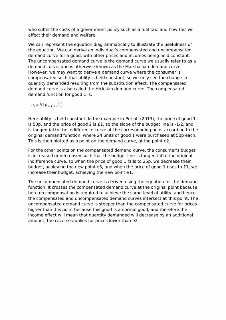
,e can represent the equation diagrammatically to illustrate the usefulness of

the equation. ,e can derive an individual’s compensated and uncompensated

demand curve for a good! with other prices and incomes being held constant. The uncompensated demand curve is the demand curve we usually refer to as a

demand curve! and is otherwise known as the $arshallian demand curve.

%owever! we may want to derive a demand curve where the consumer is

compensated such that utility is held constant! so we only see the change in

quantity demanded resulting from the substitution eect. The compensated

demand curve is also called the %icksian demand curve. The compensated

demand function for good - is"

q1= H ( p1

, p2

, U )

%ere utility is held constant. In the e#ample in erlo (/0-1! the price of good -

is 20p! and the price of good / is 3-! so the slope of the budget line is 4-*/! and

is tangential to the indierence curve at the corresponding point according to the

original demand function! where /5 units of good - were purchased at 20p each.

This is then plotted as a point on the demand curve! at the point e/.

6or the other points on the compensated demand curve! the consumer’s budget

is increased or decreased such that the budget line is tangential to the original

indierence curve! so when the price of good - falls to /2p! we decrease their

budget! achieving the new point e1! and when the price of good - rises to 3-! weincrease their budget! achieving the new point e-.

The uncompensated demand curve is derived using the equation for the demand

function. It crosses the compensated demand curve at the original point because

here no compensation is required to achieve the same level of utility! and hence

the compensated and uncompensated demand curves intersect at this point. The

uncompensated demand curve is steeper than the compensated curve for prices

higher than this point because this good is a normal good! and therefore the

income eect will mean that quantity demanded will decrease by an additional

amount+ the reverse applies for prices lower than e/.



7nother way in which the Slutsky equation is useful is that it can help us

understand 8ien goods. 9sing the equation we can see that if the second term

is larger in magnitude than the )rst term! with the income eect happening in

the opposite direction to the change in quantity demanded caused by the

substitution eect! then the change in quantity demanded will be in the same

direction as the change in price! contrary to the law of demand.

The case of a 8ien good is illustrated below



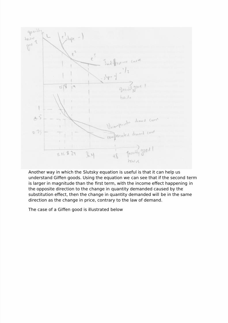
In this diagram we can see the eects of a fall in the price of p- for a normal

good" money income is held constant so a fall in the price of good - leads to the

budget line &- to shift to &/! with an optimal bundle of #’. %owever! if the

preferences of the consumer were such that they had an indierence curve of I1

then a fall in the price of good - would in fact lead to a fall in the quantity

demanded for the good. ,e can derive a demand curve for this good! where the

demand curve (i.e. the uncompensated demand curve slopes upwards.

:ndowments act as e#tra income because the consumer can sell their

endowment on" we can consider this part of their wealth or income. %owever! if

their endowment is in either of the goods being considered! then we must alter

the Slutsky equation to take into account the fact that the consumer’s eective

budget will vary with price. $oreover! the income eect can be decomposed into

two further parts" the endowment eect and the income eect. ,e denote the

endowment using the character omega! ω . 7 change in the price of the good

will pivot the budget line around the initial optimal bundle! rather than around

one of the a#is.



&ecause income does now change with price of either good as

M = p1

ω1+ p

2ω

2

;ow the Slutsky decomposition will include three components" the pure

substitution eect! pure income eect! and endowment income eect. ,e can

see this diagrammatically below"

The price of good - falls! so the budget line pivots around the initial optimal

bundle e-! and is tangential to the indierence curve I/. The budget line shifts

outwards due to the ordinary income eect! and then shifts inwards due the

endowment income eect. ,e can write this down this mathematically"

δ D i

δ p j

=δ H i

δ p j

+δ D i

δM (ω j− x j)

Consumer Behaviour, Slutsky

Documents

Transcript of Consumer Behaviour, Slutsky