Large eddy simulation of combustion using linear-eddy ... · Large eddy simulation of combustion...

Thesis for the Degree of Doctor of Philosophy

Large eddy simulation of combustionusing linear-eddy subgrid modeling

Salman Arshad

Department of Mechanics and Maritime SciencesChalmers University of Technology

Goteborg, Sweden 2019

Large eddy simulation of combustion using linear-eddy subgrid modeling

Salman Arshad

ISBN 978-91-7597-882-6

c© Salman Arshad, 2019.

Doktorsavhandlingar vid Chalmers tekniska hogskolaNy serie nr 4563ISSN 0346-718X

Department of Mechanics and Maritime SciencesChalmers University of TechnologySE–412 96 GoteborgSwedenTelephone: +46 (0)31 – 772 1000

Typeset by the author using LATEX.

Chalmers ReproserviceGoteborg, Sweden 2019

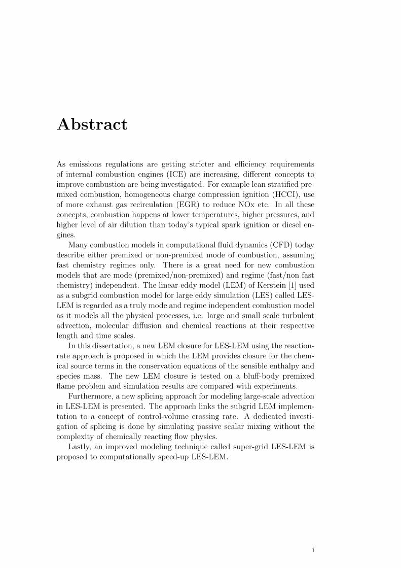
Abstract

As emissions regulations are getting stricter and efficiency requirementsof internal combustion engines (ICE) are increasing, different concepts toimprove combustion are being investigated. For example lean stratified pre-mixed combustion, homogeneous charge compression ignition (HCCI), useof more exhaust gas recirculation (EGR) to reduce NOx etc. In all theseconcepts, combustion happens at lower temperatures, higher pressures, andhigher level of air dilution than today’s typical spark ignition or diesel en-gines.

Many combustion models in computational fluid dynamics (CFD) todaydescribe either premixed or non-premixed mode of combustion, assumingfast chemistry regimes only. There is a great need for new combustionmodels that are mode (premixed/non-premixed) and regime (fast/non fastchemistry) independent. The linear-eddy model (LEM) of Kerstein [1] usedas a subgrid combustion model for large eddy simulation (LES) called LES-LEM is regarded as a truly mode and regime independent combustion modelas it models all the physical processes, i.e. large and small scale turbulentadvection, molecular diffusion and chemical reactions at their respectivelength and time scales.

In this dissertation, a new LEM closure for LES-LEM using the reaction-rate approach is proposed in which the LEM provides closure for the chem-ical source terms in the conservation equations of the sensible enthalpy andspecies mass. The new LEM closure is tested on a bluff-body premixedflame problem and simulation results are compared with experiments.

Furthermore, a new splicing approach for modeling large-scale advectionin LES-LEM is presented. The approach links the subgrid LEM implemen-tation to a concept of control-volume crossing rate. A dedicated investi-gation of splicing is done by simulating passive scalar mixing without thecomplexity of chemically reacting flow physics.

Lastly, an improved modeling technique called super-grid LES-LEM isproposed to computationally speed-up LES-LEM.

i

List of publications

This thesis is based on the following appended papers:

Paper 1

E.D. Gonzalez-Juez, A. Dasgupta, S. Arshad, M. Oevermann,D. Lignell, “Effect of the turbulence modeling in large-eddy sim-ulations of nonpremixed flames undergoing extinction and reig-nition”, 55th AIAA Aerospace Sciences Meeting, AIAA SciTechForum, AIAA 2017-0604, Grapevine, TX (2017).

Paper 2

E.D. Gonzalez-Juez, S. Arshad, M. Oevermann, S. Menon, “Turbulent-combustion closure for the chemical source terms using the linear-eddy model”, 53rd AIAA/SAE/ASEE Joint Propulsion Confer-ence, AIAA Propulsion and Energy Forum, AIAA 2017-5080,Atlanta, GA (2017).

Paper 3

S. Arshad, B. Kong, A.R. Kerstein, M. Oevermann, “A strategyfor large-scale scalar advection in large eddy simulations that usethe linear eddy sub-grid mixing model”, International Journalof Numerical Methods for Heat and Fluid Flow, Vol. 28 Issue:10, pp.2463-2479 (2018).

Paper 4

S. Arshad, E.D. Gonzalez-Juez, A. Dasgupta, S. Menon, M.Oevermann, “Subgrid reaction-diffusion closure for large eddysimulations using the linear-eddy model”, Flow, Turbulence andCombustion, In press.

iii

Acknowledgments

First of all, I would like to express my special thanks to my supervisorProfessor Michael Oevermann for his guidance, great support, all the fruitfuldiscussions and patience. My warm thanks goes to Alan Kerstein for all thegreat ideas and explanations. I am thankful to Esteban D. Gonzalez-Juezand Adhiraj Dasgupta for excellent cooperation as working together withthem was a great pleasure.

Thanks to Professor Ingemar Denbratt for giving me the chance to workon this interesting PhD project at the division of combustion and propulsionsystems.

I would like to thank the Swedish Research Council and Combustion En-gine Research Center (CERC) for financial support of the project. In addi-tion, thanks to the Swedish National Infrastructure for Computing (SNIC)at C3SE Chalmers for providing resources for the simulations.

Thanks to all my colleagues in the combustion and propulsion systemsdivision. Moreover I would like to thank my friends in Sweden for fun times.

Finally, I would thank from the bottom of my heart to my whole family.Thanks for all the support throughout my life.

v

Contents

Abstract i

List of publications iii

Acknowledgments v

Contents vii

Introduction 1

1 Model formulation 9

1.1 Introduction . . . . . . . . . . . . . . . . . . . . . . . . . . . 10

1.2 LES equations . . . . . . . . . . . . . . . . . . . . . . . . . . 10

1.3 LEM subgrid modeling inside a LES cell . . . . . . . . . . . 11

1.4 Large-scale advection modeling . . . . . . . . . . . . . . . . 14

1.4.1 New splicing algorithm . . . . . . . . . . . . . . . . . 16

1.4.2 Parallel splicing . . . . . . . . . . . . . . . . . . . . . 18

1.4.3 Splicing at inlet and outlet boundaries . . . . . . . . 19

1.5 Closure of the chemical source terms with LEM . . . . . . . 19

2 Model validation 23

2.1 Introduction . . . . . . . . . . . . . . . . . . . . . . . . . . . 24

2.2 Combustion simulations . . . . . . . . . . . . . . . . . . . . 24

2.2.1 Comparison with experiments and WSR model . . . 25

2.2.2 Comparison with traditional LES-LEM . . . . . . . . 28

2.3 Splicing investigation . . . . . . . . . . . . . . . . . . . . . . 31

2.3.1 Comparisons with experiments . . . . . . . . . . . . . 32

2.3.2 Comparison of the new and old splicing strategy . . . 33

Conclusion 35

Future work 37

vii

Contents

Summary of papers 41

References 43

Paper 1Effect of the turbulence modeling in large-eddy simulations of non-premixed flames undergoing extinction and reignition 54

Paper 2Turbulent-combustion closure for the chemical source terms usingthe linear-eddy model 72

Paper 3A strategy for large-scale scalar advection in large eddy simulationsthat use the linear eddy subgrid mixing model 92

Paper 4Subgrid reaction-diffusion closure for large eddy simulations usingthe linear-eddy model 112

viii

Introduction

Combustion has been used by humans for thousands of years for practicalpurposes of cooking food and heating homes. With the advent of the steamengine, a new use of combustion was found, i.e. to produce work. Steamengines were used particularly in railroads and steam ships. After the dis-covery of gasoline, steam engines were replaced with internal combustionengines (ICE), which are still being used extensively for e.g. transporta-tion and power generation purposes. However, tremendous use of ICE haslead to various environmental and health hazards. So modern research oncombustion in ICE has two major objectives, i.e. the optimization of com-bustion efficiency and the reduction of pollutants. In order to achieve theseobjectives, a clear understanding of the processes taking place during com-bustion is a prerequisite. This understanding will only be obtained by ajoint approach of experiments and modeling.

Turbulent combustion happening in ICE involves an interaction betweenhighly non-linear chemical reactions, turbulence and molecular mixing. Tur-bulence is characterized by a broad range of scales in spacetime, rangingfrom the smallest Kolmogorov scales to the largest flow structures charac-terized by the scales of the geometry. Computational fluid dynamics (CFD)provides useful tools to study turbulent combustion. In CFD, the governingequations are numerically solved. The computational domain is divided intoa finite number of cells on which the governing equations are discretized andthen solved. Direct numerical simulation (DNS) is a CFD tool which aimsat fully resolving the flow physics. However, DNS is currently computa-tionally affordable only for relatively simple problems and thus non-feasiblefor practical flow problems (such as ICE). In contrast, CFD approachesfor engineering problems approximate the flow physics with mathematicalformulations called turbulent combustion models. There are numerous tur-bulent combustion models available [2,3] and several studies have comparedthem, see [4–6] for a few examples.

Large eddy simulation (LES) is a popular modeling approach for simu-lating turbulent combustion. LES resolves the energy containing large-scaleturbulent motion directly and models the effect of unresolved small scales,

1

Contents

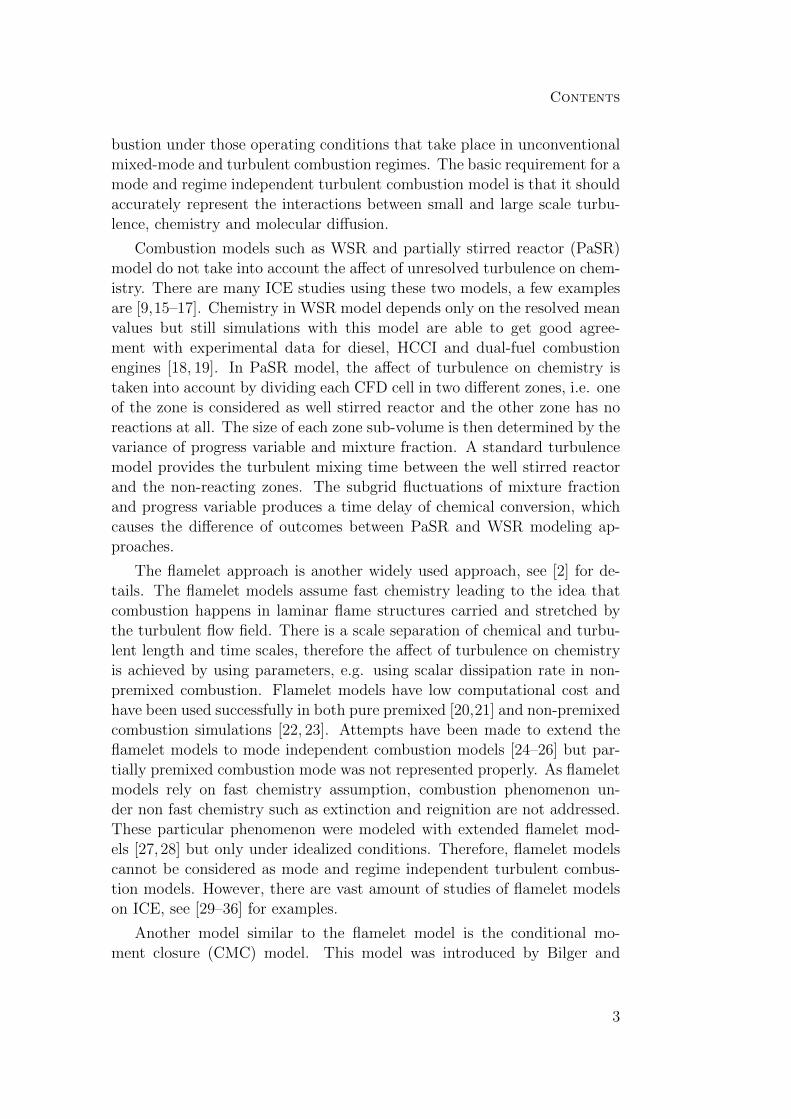
resulting in lower grid resolution requirements compared to DNS. For scalarmixing, LES has shown better predictive capabilities than Reynolds Aver-aged Navier Stokes (RANS) approaches [7]. Fig. 1 shows portion of theenergy spectrum resolved by RANS, LES and DNS respectively. In LES,large scales of the flow are separated from the smaller scales of the flowby applying a spatial filter on the governing equations. LES has showna good predictive capability in many studies related to ICE. Just a fewexamples include work done by Jhavar and Rutland [9] about the investiga-tion of cycle-to-cycle variations in homogeneous charge compression ignition(HCCI) engines using the well stirred reactor (WSR) model. Adomeit et.al [10] studied the influence of cycle-to-cycle variations of inlet conditions onthe fuel-air mixing process in a direct injection spark ignition (DISI) engine.LES simulations employing the progress variable approach (to model tur-bulent combustion) were used to study turbulent flows in diesel engines [11]and lean ethanol/air mixtures in HCCI engines [12, 13]. Other examples ofLES studies of ICE can be found in the review paper of Rutland [14].

Figure 1: Resolution of the energy spectrum by different approaches [8].Here, E(k) denotes the turbulent kinetic energy in the wavenumber (k)space.

As ICE emissions regulations are getting stricter, different concepts toimprove combustion and reducing tailpipe emissions are being studied. Forexample, to reduce NOx in spark ignition engines, lean air-fuel mixture isused and to reduce NOx in diesel engines, more exhaust gas recirculation(EGR) is being used. Other concepts of improving combustion by havinga low temperature combustion process are also being investigated. Manycurrent turbulent combustion models in CFD assume fast chemistry regimesand are aimed to describe either premixed or non-premixed modes of com-bustion. However, future engines will most likely operate at lower tempera-tures, higher pressures, and higher level of air dilution than today’s engines.So most combustion models used today might not adequately predict com-

2

Contents

bustion under those operating conditions that take place in unconventionalmixed-mode and turbulent combustion regimes. The basic requirement for amode and regime independent turbulent combustion model is that it shouldaccurately represent the interactions between small and large scale turbu-lence, chemistry and molecular diffusion.

Combustion models such as WSR and partially stirred reactor (PaSR)model do not take into account the affect of unresolved turbulence on chem-istry. There are many ICE studies using these two models, a few examplesare [9,15–17]. Chemistry in WSR model depends only on the resolved meanvalues but still simulations with this model are able to get good agree-ment with experimental data for diesel, HCCI and dual-fuel combustionengines [18, 19]. In PaSR model, the affect of turbulence on chemistry istaken into account by dividing each CFD cell in two different zones, i.e. oneof the zone is considered as well stirred reactor and the other zone has noreactions at all. The size of each zone sub-volume is then determined by thevariance of progress variable and mixture fraction. A standard turbulencemodel provides the turbulent mixing time between the well stirred reactorand the non-reacting zones. The subgrid fluctuations of mixture fractionand progress variable produces a time delay of chemical conversion, whichcauses the difference of outcomes between PaSR and WSR modeling ap-proaches.

The flamelet approach is another widely used approach, see [2] for de-tails. The flamelet models assume fast chemistry leading to the idea thatcombustion happens in laminar flame structures carried and stretched bythe turbulent flow field. There is a scale separation of chemical and turbu-lent length and time scales, therefore the affect of turbulence on chemistryis achieved by using parameters, e.g. using scalar dissipation rate in non-premixed combustion. Flamelet models have low computational cost andhave been used successfully in both pure premixed [20,21] and non-premixedcombustion simulations [22, 23]. Attempts have been made to extend theflamelet models to mode independent combustion models [24–26] but par-tially premixed combustion mode was not represented properly. As flameletmodels rely on fast chemistry assumption, combustion phenomenon un-der non fast chemistry such as extinction and reignition are not addressed.These particular phenomenon were modeled with extended flamelet mod-els [27, 28] but only under idealized conditions. Therefore, flamelet modelscannot be considered as mode and regime independent turbulent combus-tion models. However, there are vast amount of studies of flamelet modelson ICE, see [29–36] for examples.

Another model similar to the flamelet model is the conditional mo-ment closure (CMC) model. This model was introduced by Bilger and

3

Contents

Klimenko [37] and relies on the fact that a reactive scalar conditioned on aconserved scalar does not fluctuate as strongly. Therefore this model relatesthe fluctuations of all reactive scalars to a conserved scalar, e.g., mixturefraction in non-premixed combustion. The above assumption holds true ifthe flame is moderately influenced by flow then the conserved scalar doesnot fluctuate strongly and it is sufficient to use first order closure for thechemical reaction term. In this situation, CMC model is identical to theflamelet model and hence is not mode and regime independent. If the flameis heavily influenced by flow then to overcome inaccurate predictions, sec-ond order closure for the chemical reaction term is necessary which wouldresult in high computational costs. That is why ICE studies are only doneusing first order closure for the chemical source terms. De Paola et al. [38]and Bolla et al. [39] used first order CMC closure in heavy duty diesel en-gine simulations and the simulation results were in close agreement to theexperiments.

Existing mode and regime independent turbulent combustion modelsinclude transported PDF (TPDF) [40] and LES-LEM (discussed later).TPDF models use a detailed chemistry description and have been usedsuccessfully for many combustion applications. They are more computa-tionally expensive than flamelet models and thus are limited to relativelyfew reactive scalars chemistry. The mode and regime independent modelingcapabilities of TPDF models however, depend on the available micro-mixingmodels and much work has been done in the past to improve these micro-mixing models. In one-point PDF closure, interaction between turbulenceand flame micro-structures depends on modeling and this remains the keylimitation of one-point PDF closure. However, TPDF models have beensuccessfully applied to simulate various ICE concepts. Examples includework done by Zhang et al. [41] on HCCI combustion engine and Mohan andHaworth [42] on a heavy duty diesel engine.

One turbulent combustion model which has been successfully appliedto both premixed and non-premixed combustion and can be regarded as atruly mode (premixed/non-premixed) and regime (fast/non fast chemistry)independent is the linear-eddy model (LEM) of Kerstein [1] used as a subgridcombustion model for LES called LES-LEM [43,44].

Kerstein [1] developed LEM with the motivation that, in order to ac-curately represent turbulent combustion, a model should be able to repre-sent all relevant physical processes, notably turbulent advection, moleculardiffusion, and chemical reaction. LEM resolves and simulates on a one-dimensional (1D) line all these processes at their relevant length and timescales hence reducing the computational cost relative to three-dimensional(3D) DNS while retaining high resolution. The effects of realistic 3D tur-

4

Contents

bulence on the LEM scalar fields are modeled via instantaneous mappingevents using 3D scaling laws. LEM was initially formulated as a scalar mix-ing model for non-reacting flows [1] and later extended to predict reactiveflows [45]. LEM has been used both as a stand-alone tool and as an LESsubgrid combustion model (LES-LEM).

In LES-LEM, physical processes, i.e. large and small scale turbulentadvection, molecular diffusion and chemical reaction are modeled at theirrespective length and time scales. LES solves the large scale mass, mo-mentum and energy equation whereas to capture physics on the unresolvedsmall scale, LEM is used in each LES cell. LEM solves for chemical reac-tions, molecular diffusion and also models subgrid turbulent advection. LESand LEM are coupled by exchanging some information. Large-scale advec-tion in LES-LEM is modeled by lagrangian mass transfer of LEM betweenLES cells. LES-LEM has been employed in a large variety of combustionproblems [46–58]. McMurtry et al. [59] showed successful simulations ofturbulent scalar mixing employing LES-LEM. Non-premixed turbulent com-bustion simulations were done using LES-LEM by Calhoon [60] and Menonand Calhoon [61], and premixed turbulent combustion by Smith [62] andChakravarthy and Menon [63]. Spray combustion simulations using LES-LEM were performed by Pannala and Menon [64], and by incorporatingradiative heat loss and soot modeling to LES-LEM by Zimberg et al. [65].Predictions of a premixed turbulent methane/air flame using LES-LEMwere presented by Sankaran and Menon [66]. Sen and Menon employedLES-LEM simulations using artificial neural network to successfully speedup chemistry [67,68]. LES-LEM with a low-Mach-number numerical schemewas used to simulate the SANDIA non-premixed piloted methane/air flameD by Ochoa et al. [69]. Choi applied LES-LEM for simulations of a cavity-stabilized combustor [70]. A few examples of simulation on ICE includework done in KIVA for simulating a direct injection spark ignition engineusing LES-LEM [71], and an URANS-LEM method in order to investigatepressure histories in a HCCI engine [72]. Martinez et al. [73,74] studied tur-bulent combustion of hydrogen-enriched fuels by using LES-LEM. Lovett etal. [75] utilized LES-LEM for studying flame structure of bluff-body stabi-lized flames. Srinivasan et al. [76] used LES-LEM for investigating combus-tion instabilities in a continuous variable resonance combustor (CVRC) andalso performed spray combustion simulations [77]. Because of simulatingrather than modeling the interaction of turbulent advection with diffusionand chemical reactions, LES-LEM is capable of predicting extinction andreignition effects which has been demonstrated by Sen et al. in [68].

Turbulent combustion models can be used in at least two different ways[3]. One is the so-called primitive-variable method in which the models pro-

5

Contents

vide closure for the filtered or averaged thermochemical quantities, i.e. thespecies mass fractions and an energy variable such as enthalpy or temper-ature. This method is perhaps the most popular one and is typically usedwith flamelets [2], TPDF methods [78–80], and in most previous LES-LEMstudies as well. The other method is the reaction-rate approach in whichthe turbulent combustion model provides closure for the chemical sourceterms in the conservation equations of the thermochemical quantities, i.e.these class of models solve transport equations for all species and a formof the energy equation. Thus, this approach is computationally more ex-pensive than the primitive-variable method. However, the approach can beregarded as more broadly applicable as it simplifies the inclusion of morephysics into the modeling [3].

An additional advantage of using the reaction-rate approach is that itcan potentially ease the use of more than one turbulent combustion modelduring a simulation. For example, consider a combustion problem involvinga vigorously burning flame in some region in spacetime, a flame undergoingextinction-reignition in another region, and ignition in yet another region.This is a multi-physics combustion problem. Knowing the fact that turbu-lent combustion models can be more cost-effective (e.g. in terms of accuracyand computational cost) for a particular type of physics but not necessarilyfor other physics, it becomes desirable to use one particularly suitable modelfor one region in spacetime and other suitable models in other regions. Thepotential for such an approach to lead to more cost-effective combustionsimulations is beginning to be recognized [81,82]. This is the case not onlyin the combustion community but, for instance, in the multi-phase-flow com-munity as well [83]. Within this hybrid framework, the primitive-variablemethod runs into difficulty that turbulent combustion models handle theturbulent transport in different ways. In comparison, the reaction-rate ap-proach does not run into this problem as it solves for the conservationequations of the thermochemical quantities. Furthermore, the reaction-rateapproach isolates modeling errors due to the turbulent combustion modelin the chemical source terms, simplifying as well the comparison of errorsfrom different models.

The primitive-variable approach is standard for previous LES-LEM im-plementation so it is valuable then to explore how well a new LEM closurewith the reaction-rate approach performs. This thesis introduces a newLEM closure for LES-LEM using the reaction-rate approach. In this clo-sure, a low-Mach-number formulation of LES equations for mass, momen-tum, sensible enthalpy and species mass are solved in Eulerian form on a3D LES grid. LEM solves for temperature and species mass on the 1D lineinside each LES cell. LEM solves chemical reactions and molecular diffusion

6

Contents

and the subgrid turbulent advection is modeled by LEM by stochastic re-arrangement events called triplet maps. The triplet maps represent action ofturbulent eddies on the LEM scalars. Another element of the present LES-LEM formulation is modeling of large-scale advection, for which the splicingalgorithm is used since it has proven to be robust for practical combustionimplementations. The splicing algorithm cuts and pastes the end portionsof the 1D arrays of the adjacent LES cells to emulate a Lagrangian type ofmass transfer. Decisions of how much to cut and paste are based on valuesof the mass fluxes across the faces of LES computational cells. For example,if the mass flux at a given face of cell A is large and directed from cell A tocell B, a large portion of the 1D array in A will be cut and then pasted ontoone of the two endpoints of the array in B. If this mass flux were small, asmall portion would be cut and pasted. A new splicing strategy based onan ordered flux of spliced LEM segments is presented here in this thesis.The principle is that low-flux segments have less momentum than high-fluxsegments and therefore are displaced less than high-flux segments. Thisstrategy affects the order of both inflowing and outflowing LEM segmentsof a LES cell. In the present LES-LEM formulation, during each LES timestep LES provides information needed to advance the LEM solution andLEM in return provides chemical source terms to LES. These source termsare then used in LES equations for sensible enthalpy and species mass.

In this thesis, LES-LEM predictions with the new closure for a bluff-body stabilized combustor are compared with experiments, WSR model anda traditional LES-LEM study employing the primitive-variable approach.The bluff-body stabilized combustor is a standard test case for the evalua-tion of turbulent premixed combustion models which has been investigatedextensively in the past. The present work makes use of unstructured meshesand a pressure-based approach, both of which are favorable in industry. Itis shown that current LES-LEM implementation is robust. Focus is alsoput on an important part of LES-LEM, i.e. splicing. A dedicated investi-gation of splicing is done by simulating turbulent passive scalar mixing andby comparing the new splicing strategy with an old one.

This thesis has two chapters. The first chapter describes the modelformulation of LES-LEM using the reaction-rate approach. The secondchapter focuses on the combustion simulations using LES-LEM and thededicated investigation of splicing by doing the mixing simulations.

7

Chapter 1

Model formulation

9

Chapter 1. Model formulation

1.1 Introduction

This chapter describes the LES-LEM model in detail. The LES-LEM modelis composed of the following elements: the LES equations (section 1.2),the LEM modeling inside a LES cell (section 1.3), the large-scale advectionmodeling by splicing (section 1.4) and for the current formulation the closureof the chemical source terms and exchange of information between the LEMand the LES (section 1.5).

The governing conservation equations for mass and momentum are:

∂ρ

∂t+∂(ρui)

∂xi= 0 , (1.1)

∂ρui∂t

+∂(ρujui)

∂xj= − ∂p

∂xi+

∂

∂xj(τji) . (1.2)

Here ρ denotes the density, p the pressure, ui is the velocity component inspatial direction i and τji the viscous stress tensor.

In LES, the three common filters include a cut-off filter in spectral space,a box (top-hat) filter in physical space and a Gaussian filter in physicalspace [3]. The current work uses the implicit top-hat filter.

1.2 LES equations

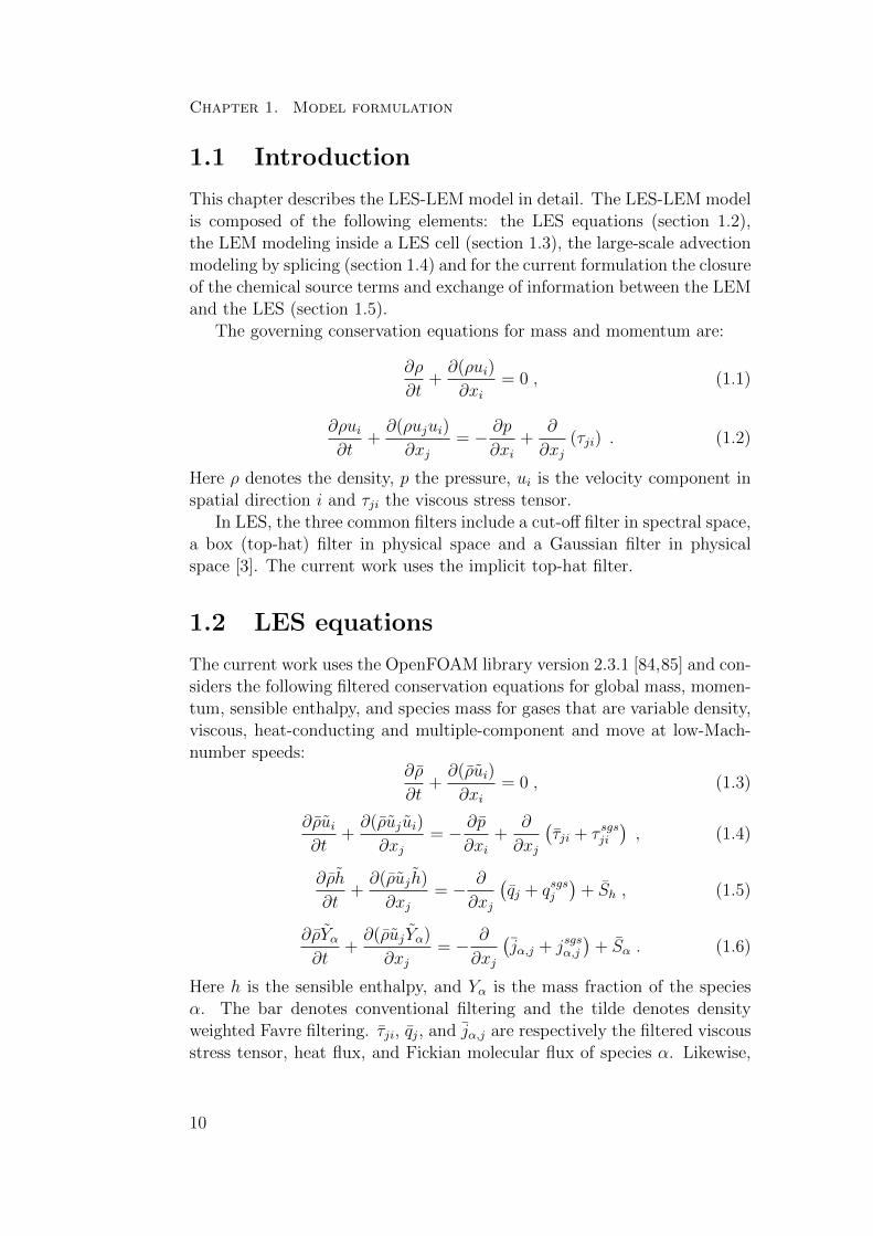
The current work uses the OpenFOAM library version 2.3.1 [84,85] and con-siders the following filtered conservation equations for global mass, momen-tum, sensible enthalpy, and species mass for gases that are variable density,viscous, heat-conducting and multiple-component and move at low-Mach-number speeds:

∂ρ

∂t+∂(ρui)

∂xi= 0 , (1.3)

∂ρui∂t

+∂(ρujui)

∂xj= − ∂p

∂xi+

∂

∂xj

(τji + τ sgsji

), (1.4)

∂ρh

∂t+∂(ρujh)

∂xj= − ∂

∂xj

(qj + qsgsj

)+ Sh , (1.5)

∂ρYα∂t

+∂(ρujYα)

∂xj= − ∂

∂xj

(jα,j + jsgsα,j

)+ Sα . (1.6)

Here h is the sensible enthalpy, and Yα is the mass fraction of the speciesα. The bar denotes conventional filtering and the tilde denotes densityweighted Favre filtering. τji, qj, and jα,j are respectively the filtered viscousstress tensor, heat flux, and Fickian molecular flux of species α. Likewise,

10

1.3. LEM subgrid modeling inside a LES cell

τ sgsji , qsgsj , and jsgsα,j are the subgrid viscous stress tensor, heat flux, andmolecular flux of species α, all of which need closure. These conservationequations are complemented with the equation of state for ideal gases

p = ρRm

N∑

α=1

YαT

Wα

, (1.7)

where Wα is the molecular weight of species α and Rm is the universal gasconstant. The averaged caloric equation of state is given as,

h = h(T ) =∑

α

Yαhα(T ) (1.8)

with hα(T ) given by the NASA polynomials.

The terms τ sgsij , qsgsj , and jsgsα,j are the subgrid stress tensor, heat flux,and mass flux of species α. They are closed with

τ sgsij = −2µsgs(Sij −

δij3Skkδij

), (1.9)

qsgsj = −µsgs

ρ

∂hs∂xj

, (1.10)

jsgsα,j = −µsgs

ρ

∂Yα∂xj

. (1.11)

µsgs is computed with OpenFOAM’s implementation of Yoshizawa & Ho-riuti’s one-equation eddy model [86].

1.3 LEM subgrid modeling inside a LES cell

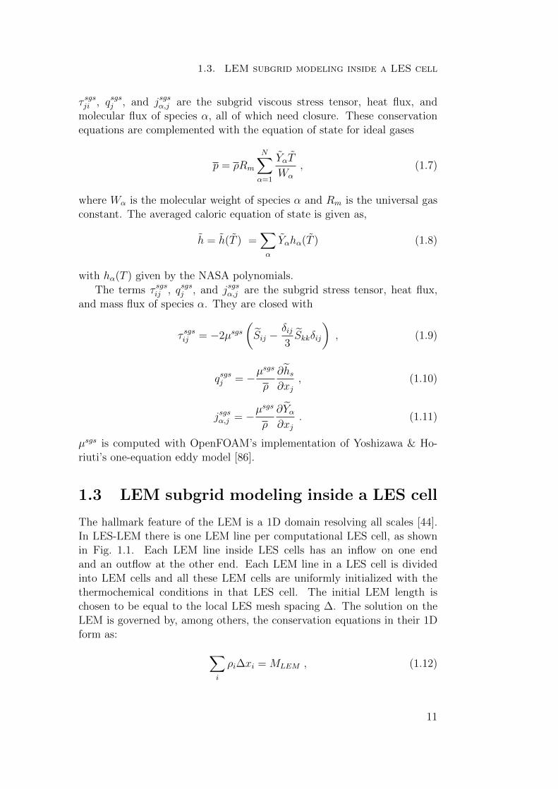
The hallmark feature of the LEM is a 1D domain resolving all scales [44].In LES-LEM there is one LEM line per computational LES cell, as shownin Fig. 1.1. Each LEM line inside LES cells has an inflow on one endand an outflow at the other end. Each LEM line in a LES cell is dividedinto LEM cells and all these LEM cells are uniformly initialized with thethermochemical conditions in that LES cell. The initial LEM length ischosen to be equal to the local LES mesh spacing ∆. The solution on theLEM is governed by, among others, the conservation equations in their 1Dform as:

∑

i

ρi∆xi = MLEM , (1.12)

11


Figure 1.1: LES-LEM simulations use a 1D domain (in black) consisting ofa stack of LEM cells per computational LES cell (in red) [87]. Note thatthe LEM domains have no assigned orientation relative to the underlyingcoordinate system.

∂T

∂t= −∂qx

∂x+ ST , (1.13)

∂Yα∂t

= −∂jα,x∂x

+ Sα , (1.14)

where MLEM is the total mass in a LEM line, the summation (index i) isdone over all cells of the LEM domain, the x coordinate is parallel to the 1Dline, and ST is the heat-source term in the temperature equation. Constantpressure is assumed on the LEM which allows updating of the LEM density.Unity Lewis number is used to compute qx and jα,x.

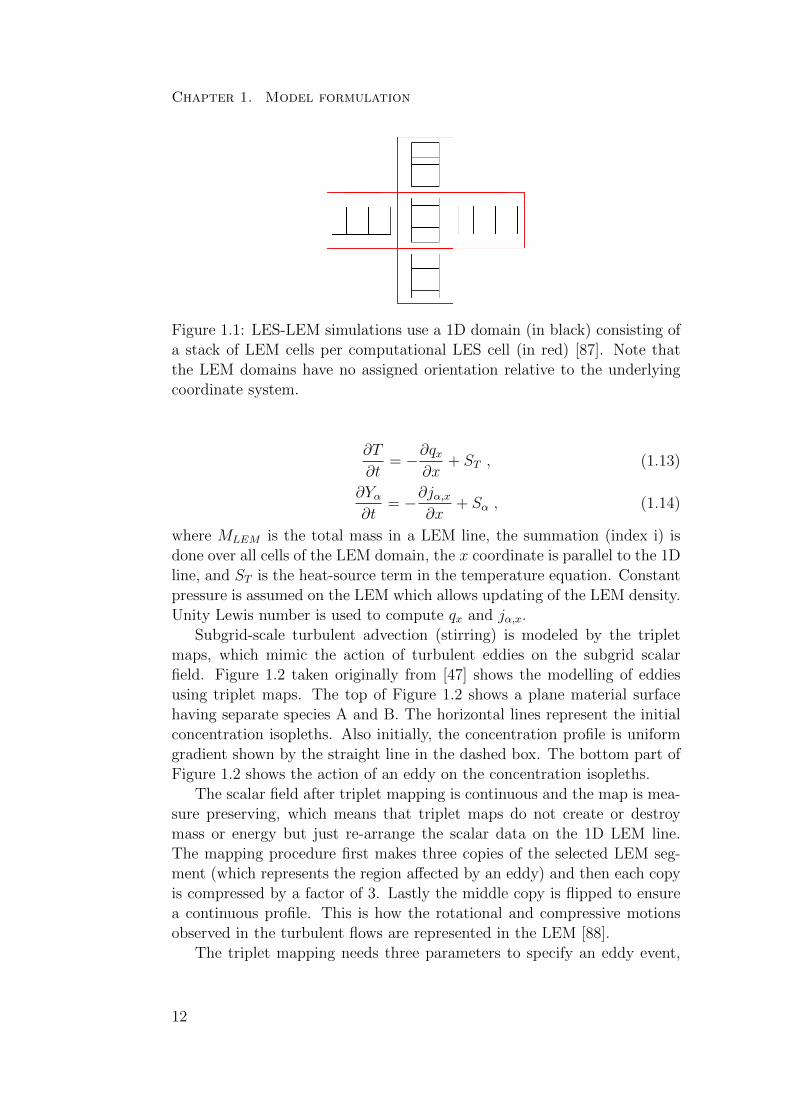
Subgrid-scale turbulent advection (stirring) is modeled by the tripletmaps, which mimic the action of turbulent eddies on the subgrid scalarfield. Figure 1.2 taken originally from [47] shows the modelling of eddiesusing triplet maps. The top of Figure 1.2 shows a plane material surfacehaving separate species A and B. The horizontal lines represent the initialconcentration isopleths. Also initially, the concentration profile is uniformgradient shown by the straight line in the dashed box. The bottom part ofFigure 1.2 shows the action of an eddy on the concentration isopleths.

The scalar field after triplet mapping is continuous and the map is mea-sure preserving, which means that triplet maps do not create or destroymass or energy but just re-arrange the scalar data on the 1D LEM line.The mapping procedure first makes three copies of the selected LEM seg-ment (which represents the region affected by an eddy) and then each copyis compressed by a factor of 3. Lastly the middle copy is flipped to ensurea continuous profile. This is how the rotational and compressive motionsobserved in the turbulent flows are represented in the LEM [88].

The triplet mapping needs three parameters to specify an eddy event,

12

1.3. LEM subgrid modeling inside a LES cell

Figure 1.2: Schematics of the effect of an eddy [47]

i.e. an eddy location x0 within the LEM domain, eddy length l, and aneddy rate λ per unit domain length. The eddy location x0 is sampled in astochastic way from a uniform distribution.

If f(l) denotes the probability density function of the eddy sizes, thenthe turbulent diffusivity DT is given by [89]:

DT =

∫ lmax

lp

2

27λl3f(l)dl , (1.15)

where lp and lmax are the smallest and the largest unresolved length scalescharacterizing the turbulence, and are specified by the user. Here lp is takenas the Kolmogorov length scale η and lmax = ∆. The turbulent diffusivityDT scales with l4/3 [89–91] resulting in:

f(l) =5

3

l−8/3

η−5/3 −∆−5/3, (1.16)

An estimate for the Kolmogorov length scale is given by

η = Nη∆

Re3/4∆

, (1.17)

13


with Nη being a model constant, and Re∆ the subgrid Reynolds number:

Re∆ =usgs∆

ν, (1.18)

where ν is the kinematic viscosity and usgs is the characteristic subgridvelocity fluctuation obtained from the LES subgrid turbulent kinetic energyksgs as usgs =

√2ksgs/3.

The eddy rate λ with unit (length x time)-1 is obtained by insertingEq. 1.16 in to Eq. 1.15 as shown in [89]

λ =54

5

νRe∆

Cλ∆3

(∆η

)5/3

− 1

1−(η∆

)4/3, (1.19)

with Cλ being a model constant. The average time interval between tripletmaps is:

∆tstir =1

λlLEM. (1.20)

where lLEM is the LEM domain length and the actual eddy occurrencesare sampled from a Poisson process. The sampling rejected the eddies thatextend beyond the LEM domain boundary. The values of Cλ = 1 andNη = 1.1 are used. These values were chosen to ensure that triplet mapsare being observed during the simulation.

1.4 Large-scale advection modeling

On the LES, large-scale advection is simply the resolved flow which trans-ports/advects small-scale structures across LES cell boundaries. As small-scale structures are represented on the LEM, a splicing procedure representslarge-scale advection for the LEMs. Splicing satisfies conservation of massand transports mass across LES cell faces in a Lagrangian way. Splicingaccounts for mass fluxes across LES cell faces and is implemented via La-grangian transport of LEM cells between LES control volumes. This methodrequires three quantities:

1. The magnitude of mass to be transported across each LES cell face,

2. The direction of mass transport on each LES cell face i.e. outflux orinflux,

3. An algorithm for ordering of the splicing operations.

14

1.4. Large-scale advection modeling

Total mass to be transferred across each LES cell face has two contributions,a subgrid mass due to the unresolved velocity fluctuation and a resolvedmass due to the resolved velocity. The subgrid mass contribution is givenby:

Msgs =∆tALESusgs

VLESMLEM , (1.21)

where ALES is the LES face area. VLES and MLEM denote the LES cellvolume of splicing donor and the total mass of LEM line of splicing donor,respectively. The direction of the subgrid mass contribution is chosen ran-domly.

The resolved mass contribution for total splicing mass is given in analogyto Eq. 1.21 by:

Mres =∆tALESuLES

VLESMLEM , (1.22)

where uLES is the LES resolved velocity on the LES cell face. The directionof the resolved mass contribution is given by the direction of uLES.

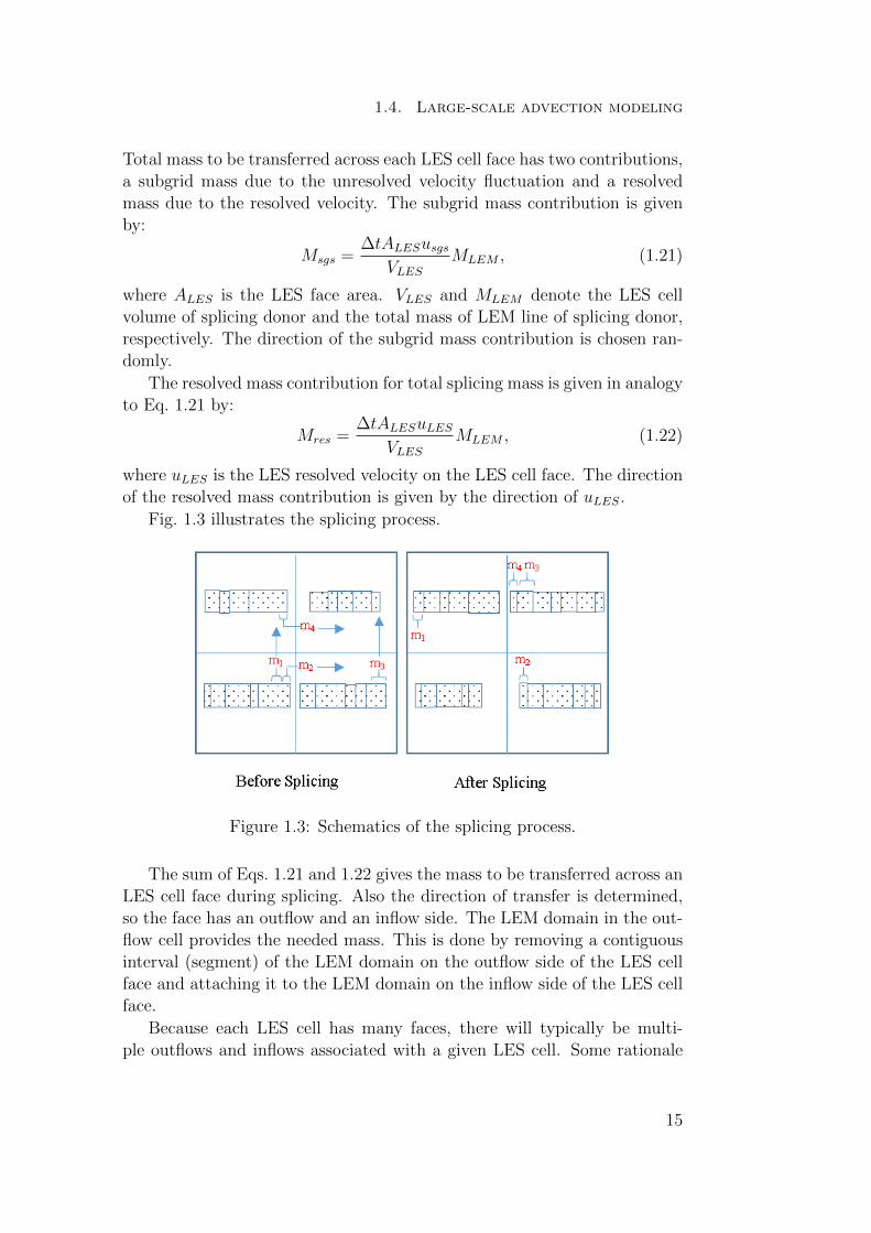
Fig. 1.3 illustrates the splicing process.

Figure 1.3: Schematics of the splicing process.

The sum of Eqs. 1.21 and 1.22 gives the mass to be transferred across anLES cell face during splicing. Also the direction of transfer is determined,so the face has an outflow and an inflow side. The LEM domain in the out-flow cell provides the needed mass. This is done by removing a contiguousinterval (segment) of the LEM domain on the outflow side of the LES cellface and attaching it to the LEM domain on the inflow side of the LES cellface.

Because each LES cell has many faces, there will typically be multi-ple outflows and inflows associated with a given LES cell. Some rationale

15


is needed to determine the locations and sequencing of the removals andattachments of the segments crossing the various faces of a given LES cell.

This depends first on the chosen structure of the LEM domain. Topo-logically, the choices are a loop, corresponding to periodic boundary condi-tions, or a line segment. Here, as in most of the cited previous work, a linesegment is used, with input and output sites at the respective endpointsof the line segment. This is a desirable choice because it tends to enforceconsistency of the residence time of LEM fluid elements, which extendsfrom the time of attachment to the LEM domain to the time of eventualremoval. This point is illustrated by considering the alternative choice ofattaching and removing fluxed segments at the same endpoint. Then theresidence-time distribution would be highly skewed, with a strong peak atshort residence time and a long tail reflecting fluid retained for a long timenear the other endpoint, which is effectively an unphysical stagnation point.This is not only counter-intuitive, but introduces model artifacts. In Eule-rian schemes, the Courant-Friedrichs-Lewy (CFL) constraint is associatedwith the requirement that fluid should not be algorithmically propagatedthrough multiple control volumes during one time step. This is a numericalinstability mechanism as well as unphysical. Attachment and removal atthe same LEM endpoint could propagate some fluid through multiple con-trol volumes during one time step because the total number of attachmentsand removals per LEM domain equals the number of LES cell faces, whichis six in a Cartesian mesh and typically more in an unstructured mesh, al-lowing a possible ‘bucket brigade’ scenario. Avoidance of this would requiretime step reduction far below the permissible CFL time step for an Euleriantransport scheme.

The mean residence time is dictated by the LES-prescribed mass-fluxtime history, so the degree of freedom available to avoid this artifact is theresidence-time distribution, which should be as narrow as possible to min-imize residence-time fluctuations. Designating each LEM domain endpointas solely an input or an output location assures that fluid must pass throughthe domain between its attachment and removal times, thus avoiding theshort-residence-time scenario.

1.4.1 New splicing algorithm

The new splicing approach links the subgrid LEM implementation to theconcept of control-volume crossing rate. The direction of the crossing rateis implied by the direction of the LES-prescribed mass fluxes. High fluximplies high crossing rate, corresponding to high displacement per timestep, and vice versa. High flux also implies the transfer of a relatively large

16

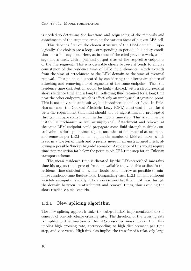
1.4. Large-scale advection modeling

mass of the LEM domain across an LES cell face. It follows that largermass transfers undergo more displacement, and vice versa, as illustrated inFig. 1.4.

Figure 1.4: Principle of the new splicing algorithm

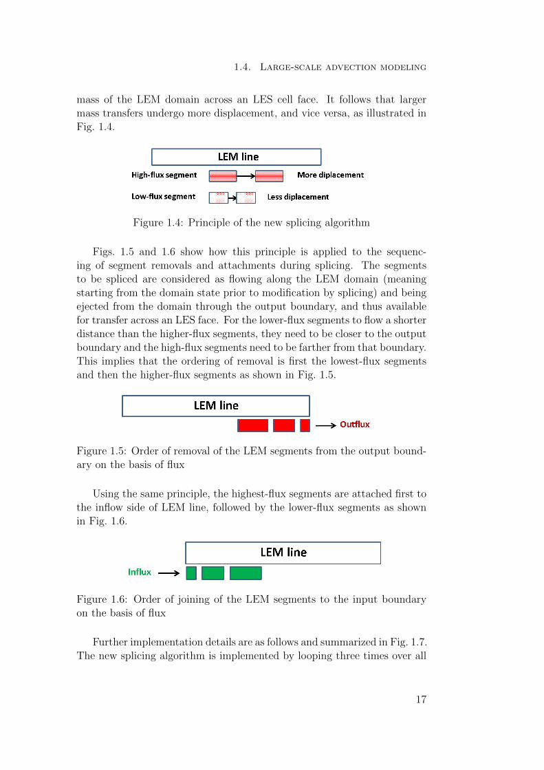
Figs. 1.5 and 1.6 show how this principle is applied to the sequenc-ing of segment removals and attachments during splicing. The segmentsto be spliced are considered as flowing along the LEM domain (meaningstarting from the domain state prior to modification by splicing) and beingejected from the domain through the output boundary, and thus availablefor transfer across an LES face. For the lower-flux segments to flow a shorterdistance than the higher-flux segments, they need to be closer to the outputboundary and the high-flux segments need to be farther from that boundary.This implies that the ordering of removal is first the lowest-flux segmentsand then the higher-flux segments as shown in Fig. 1.5.

Figure 1.5: Order of removal of the LEM segments from the output bound-ary on the basis of flux

Using the same principle, the highest-flux segments are attached first tothe inflow side of LEM line, followed by the lower-flux segments as shownin Fig. 1.6.

Figure 1.6: Order of joining of the LEM segments to the input boundaryon the basis of flux

Further implementation details are as follows and summarized in Fig. 1.7.The new splicing algorithm is implemented by looping three times over all

17


Start

i = 1

i ≤ nf

mres + msgs

i + 1 True

j = 1

j ≤ ncells

Outflux splicing ascending order

j + 1True

False

k = 1

k ≤ ncells

Influx splicing descending

order

k + 1True

FalseEnd

False

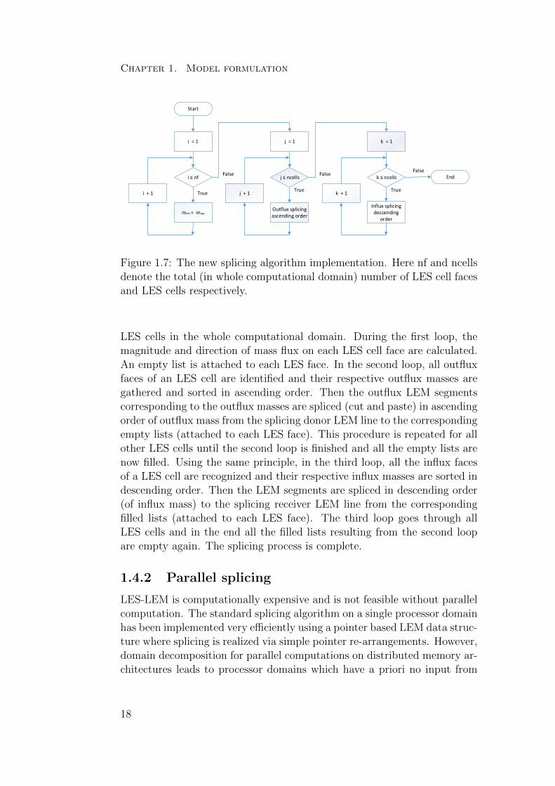
Figure 1.7: The new splicing algorithm implementation. Here nf and ncellsdenote the total (in whole computational domain) number of LES cell facesand LES cells respectively.

LES cells in the whole computational domain. During the first loop, themagnitude and direction of mass flux on each LES cell face are calculated.An empty list is attached to each LES face. In the second loop, all outfluxfaces of an LES cell are identified and their respective outflux masses aregathered and sorted in ascending order. Then the outflux LEM segmentscorresponding to the outflux masses are spliced (cut and paste) in ascendingorder of outflux mass from the splicing donor LEM line to the correspondingempty lists (attached to each LES face). This procedure is repeated for allother LES cells until the second loop is finished and all the empty lists arenow filled. Using the same principle, in the third loop, all the influx facesof a LES cell are recognized and their respective influx masses are sorted indescending order. Then the LEM segments are spliced in descending order(of influx mass) to the splicing receiver LEM line from the correspondingfilled lists (attached to each LES face). The third loop goes through allLES cells and in the end all the filled lists resulting from the second loopare empty again. The splicing process is complete.

1.4.2 Parallel splicing

LES-LEM is computationally expensive and is not feasible without parallelcomputation. The standard splicing algorithm on a single processor domainhas been implemented very efficiently using a pointer based LEM data struc-ture where splicing is realized via simple pointer re-arrangements. However,domain decomposition for parallel computations on distributed memory ar-chitectures leads to processor domains which have a priori no input from

18

1.5. Closure of the chemical source terms with LEM

neighboring processor domains. If splicing is not done correctly (e.g. by asimplified cell averaged approach) at processor boundaries, it can lead tounphysical results.

In order to perform splicing across processor boundaries, LEM linesacross processor boundaries (called ghost LEM lines) are copied to theneighboring processor. Then splicing is performed between LEM lines thatare next to the boundary and the ghost LEM lines by each processor.

1.4.3 Splicing at inlet and outlet boundaries

For LES cells at the inlet boundary, inlet mass needs to be added to theirrespective LEM lines. This inlet spliced mass is calculated using the sameEqs. 1.21 and 1.22 and is added on the influx side of the LEM line. Theremaining properties of this added fluid are taken from the inlet bound-ary. For inlet splicing mass calculations, the direction of the subgrid masscontribution (Eq. 1.21) is taken to be influx.

For the outlet boundaries, the calculated outlet splicing mass is removedfrom the outflux side of the LEM line. For outlet splicing mass calculations,the direction of the subgrid mass contribution (Eq. 1.21) is taken to beoutflux.

1.5 Closure of the chemical source terms with

LEM

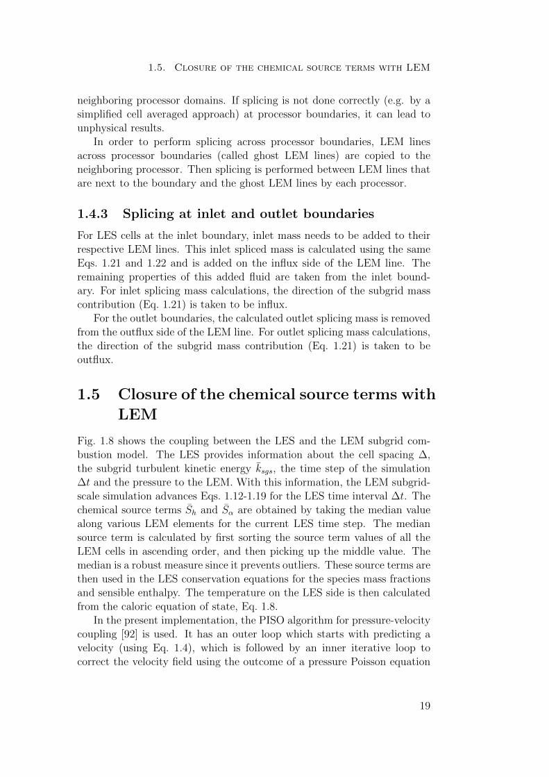
Fig. 1.8 shows the coupling between the LES and the LEM subgrid com-bustion model. The LES provides information about the cell spacing ∆,the subgrid turbulent kinetic energy ksgs, the time step of the simulation∆t and the pressure to the LEM. With this information, the LEM subgrid-scale simulation advances Eqs. 1.12-1.19 for the LES time interval ∆t. Thechemical source terms Sh and Sα are obtained by taking the median valuealong various LEM elements for the current LES time step. The mediansource term is calculated by first sorting the source term values of all theLEM cells in ascending order, and then picking up the middle value. Themedian is a robust measure since it prevents outliers. These source terms arethen used in the LES conservation equations for the species mass fractionsand sensible enthalpy. The temperature on the LES side is then calculatedfrom the caloric equation of state, Eq. 1.8.

In the present implementation, the PISO algorithm for pressure-velocitycoupling [92] is used. It has an outer loop which starts with predicting avelocity (using Eq. 1.4), which is followed by an inner iterative loop tocorrect the velocity field using the outcome of a pressure Poisson equation

19


LES

LEMYα(x), T(x), ρ(x), p

Correction

Splicing

ρ, ui, p,

h, Yα, ksgs

Sh, Sα

Yα, T

ksgs, ui

ksgs, Δ, Δt, p_ _

_

_

_

_ _

~

~ ~ ~

~ ~

_

Figure 1.8: Coupling between the LES and the LEM subgrid model.

obtained by fulfilling the continuity equation. In the inner iterative loop,the LES density is obtained from the equation of state Eq. 1.7. Splicing isdone with the correct LES velocity resulting from the PISO loop.

The last step shown in Fig. 1.8 is to correct the temperatures and thespecies mass fractions in the LEM domains to take into account the fact thatthe convection due to the solution of Eqs. 1.3-1.6 differs from that of thesplicing algorithm. This difference is not surprising because the convectionof species by the solution of Eq. 1.6 differs from that produced by the splicingin at least two ways. First, the solution of Eq. 1.6 numerically smearsthe species in a way that the splicing is not prone to because the splicingcorresponds to diffusion-free advection in a Lagrangian way. Second, thesplicing produces an artifact [93] that the solution of Eq. 1.6 is not proneto.

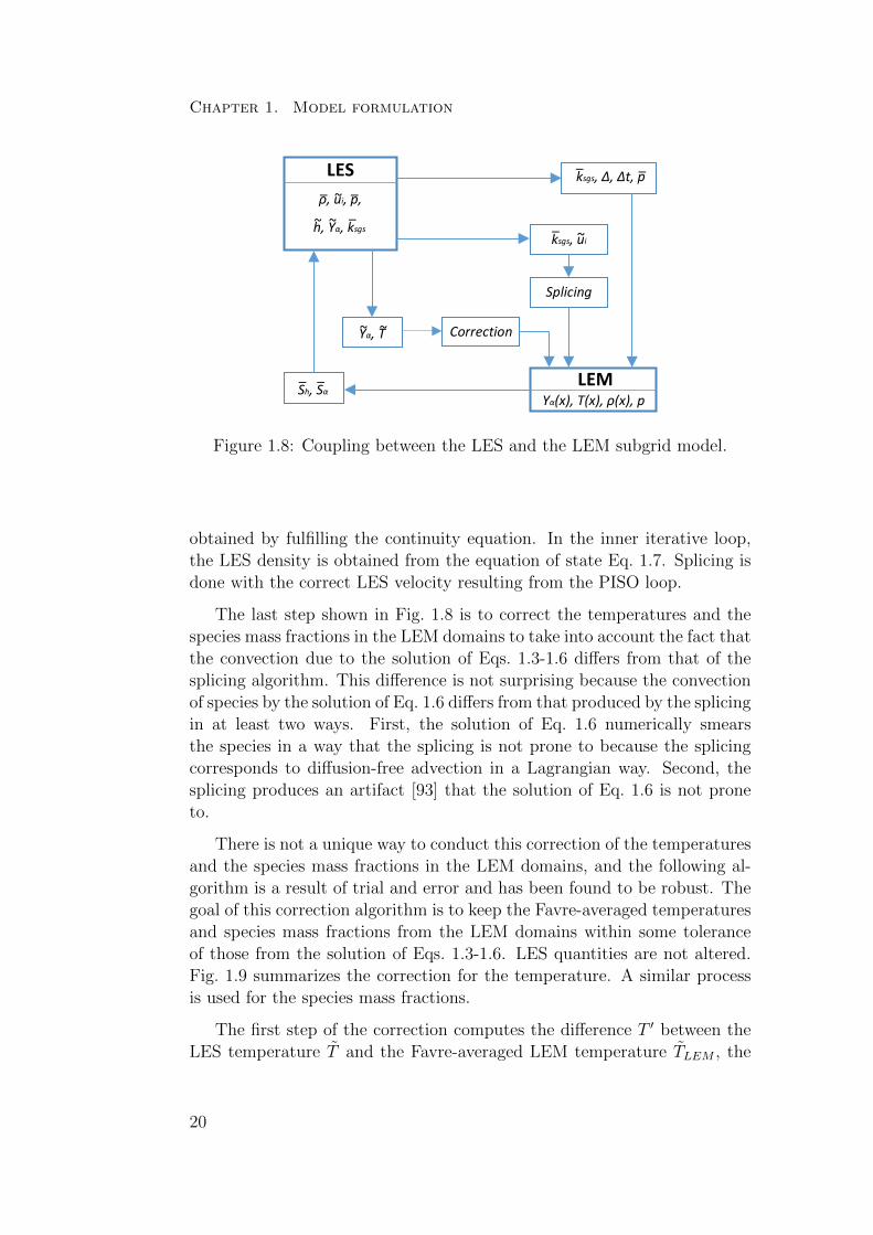
There is not a unique way to conduct this correction of the temperaturesand the species mass fractions in the LEM domains, and the following al-gorithm is a result of trial and error and has been found to be robust. Thegoal of this correction algorithm is to keep the Favre-averaged temperaturesand species mass fractions from the LEM domains within some toleranceof those from the solution of Eqs. 1.3-1.6. LES quantities are not altered.Fig. 1.9 summarizes the correction for the temperature. A similar processis used for the species mass fractions.

The first step of the correction computes the difference T ′ between theLES temperature T and the Favre-averaged LEM temperature TLEM , the

20

1.5. Closure of the chemical source terms with LEM

Start

TrueFalse

End

iT += T

T = ~T - LEM~T

≤ /20?~TT | |

~LEMT = ΣiρiΔxiTi

ΣiρiΔxi

i = 1,…,nLEM

Figure 1.9: Steps of correcting the temperature in a LEM domain. Here Tiis the temperature of LEM cell i and nLEM is the total number of LEM cells.The temperature difference T ′ is a difference between the LES temperatureT and the Favre-averaged LEM temperature TLEM .

latter of which is obtained via:

TLEM =

∑i ρi∆xiTi∑i ρi∆xi

, (1.23)

where Ti denotes the LEM cell temperature, and summation (index i) isover all cells of the LEM line. In the second step, T ′ is added to eachTi and this results in updated TLEM . If the new updated difference T ′ iswithin a specified tolerance, the correction is stopped, otherwise the updateddifference T ′ is added again to each Ti and the aforementioned steps arerepeated.

It is important to highlight a distinctive conceptual feature of the presentLEM closure using the chemical source terms. It is common in LES to makea sharp distinction between the closure of diffusive processes (micro-mixing)and reaction. This is evident by noticing that in Eqs. 1.3-1.6 separate closure

21


is needed for, on one hand, qj and jα,j, and, on the other hand, Sh and Sα.However, a more realistic picture is that diffusive and reacting processes areclosely coupled at the subgrid level (meaning reaction and diffusive termscan be of the same order), for example, in some premixed flames. Now, withLEM Sh and Sα are computed as explained above using a 1D structure thatrepresents both reaction and diffusion. Thus, it is perhaps more accurate tosay that the present closure, although given for Sh and Sα, is not a closurefor subgrid reaction, but for subgrid reaction-diffusion processes, i.e. withproper resolution the LEM is capable of fully resolving flame structuresin 1D. This is why the present LEM closure can also be called as subgridreaction-diffusion closure with LEM.

22

Chapter 2

Model validation

23

Chapter 2. Model validation

2.1 Introduction

This chapter presents in section 2.2, the combustion simulations performedwith the present LES-LEM formulation. The dedicated splicing investiga-tion is discussed in section 2.3.

2.2 Combustion simulations

The experimental setup of the bluff-body stabilized combustor [94–96] calledVolvo combustor from now on consists of a rectilinear channel, with an inletsection where air and (gaseous) propane mix before entering a honeycomb,and a downstream section where the premixed reactants burn in a flame thatgets stabilized downstream of a wedge [94]. The cross section of the wedgeis an equilateral triangle with side of 40 mm. The end of the downstreamsection is connected to a round exhaust duct with a cross sectional areaabout 3.4 times larger than that of the channel [97]. Atmospheric conditionsare used.

The computational domain used for the current work is shown in Fig. 2.1and has the following geometric parameters: h1 = 40 mm, h2 = h1sin60,xmin = -820 mm, xmax = 680 mm, ymin = -60 mm, ymax = 60 mm, and aspanwise length of 40 mm. The honeycomb is ignored as done in previousCFD studies. The pressure gradient normal to the inlet plane is set tozero. No turbulent fluctuations are imposed at the inlet because the regionof interest is downstream of the wedge which is responsible for generationof strong turbulence. All walls are modeled as no-slip and non-adiabatic.At the outlet, velocity, temperature and species are set to a zero-normal-gradient condition or a fixed value, depending on the direction of the flow.Pressure is dealt with a similar way at the outlet. Cyclic boundary condi-tions are used in the z-direction. A non-uniform 3D mesh with 77400 cellsis used as well as a tetrahedral 3D mesh with 101134 cells. With the formera time step of 1x10−6 s is used, while a time step of 4x10−7 s is used withthe latter mesh.

The conservation Eqs. 1.3-1.6 are solved with an adaptation of reacting-Foam which is the standard solver of the OpenFOAM library for chemicallyreacting flow. This solver is transient, pressure-based and can handle un-structured meshes [98]. A low-Mach-number assumption is used as done inreactingLMFoam [99,100] by splitting the pressure into a fluid-mechanical-induced pressure and a thermodynamic pressure, the latter of which is spa-tially constant and which is used to evaluate the equation of state. Asa result, acoustic waves are eliminated from the solution. The time dis-cretization is done with a second-order backward-differencing scheme that

24

2.2. Combustion simulations

Figure 2.1: Schematic of the Volvo test problem.

Table 2.1: Summary of the simulation settings for case 1

Simulation No. Denomination Mesh Cλ Correction

1 WSR model Hexahedral NA NA

2 LES-LEM baseline Hexahedral 1 on

3 LES-LEM Cλ = 10 Hexahedral 10 on

4 LES-LEM correction off Hexahedral 1 off

5 LES-LEM tetra Tetrahedral 1 on

6 PaSR tetra Tetrahedral NA NA

uses the current and previous two time step values. OpenFOAM’s limitedlinear differencing scheme is used for the convective and diffusive fluxes. µsgs

is computed with OpenFOAM’s implementation of Yoshizawa & Horiuti’sone-equation eddy model [86].

Of the various operating conditions of the Volvo test problems, the oneconsidered for the present work is the so-called case 1. In case 1, the inletconditions are 288 K temperature, 17 m/s velocity, and 0.61 equivalenceratio. Tab. 2.1 summarizes the various simulations conducted for the presentstudy. A single-step chemical reaction mechanism is used.

2.2.1 Comparison with experiments and WSR model

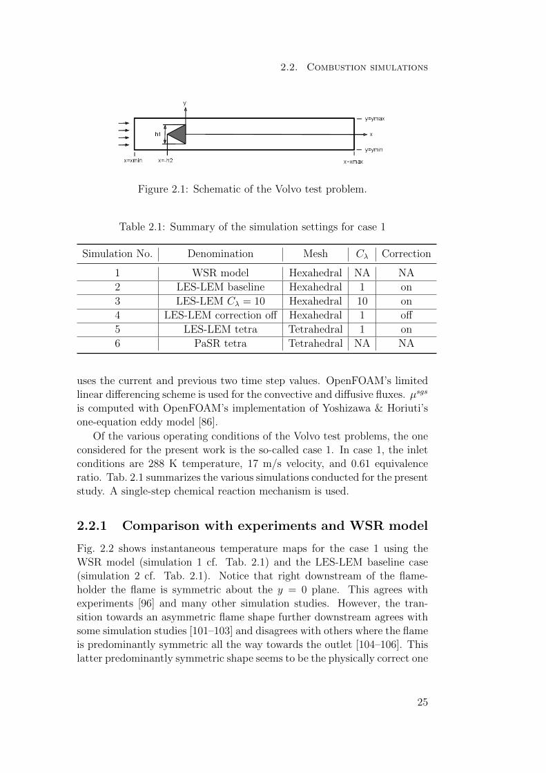
Fig. 2.2 shows instantaneous temperature maps for the case 1 using theWSR model (simulation 1 cf. Tab. 2.1) and the LES-LEM baseline case(simulation 2 cf. Tab. 2.1). Notice that right downstream of the flame-holder the flame is symmetric about the y = 0 plane. This agrees withexperiments [96] and many other simulation studies. However, the tran-sition towards an asymmetric flame shape further downstream agrees withsome simulation studies [101–103] and disagrees with others where the flameis predominantly symmetric all the way towards the outlet [104–106]. Thislatter predominantly symmetric shape seems to be the physically correct one

25


Figure 2.2: Case 1 instantaneous temperature maps with the WSR model(top), the LES-LEM baseline case (center), and a LES-LEM case withoutthe correction (bottom), cf. Tab. 2.1.

for the present boundary conditions because many of the most recent sim-ulation studies show this shape [107–111]. The use of a low-Mach-numberformulation instead of a fully-compressible one [109] in the present studymay be the cause for the transition from symmetric to asymmetric flameshape seen in the present simulations. Furthermore, it must be stressedthat, from the open literature, it is unclear how the flame looks like close tothe outlet in the experiments. Fig. 2.2 also compares the effect of the cor-rection step, cf. Figs. 1.8 and 1.9. Notice in Fig. 2.2 that by not using thiscorrection there is an artificial extinction of the flame. Thus, the correctionstep or some alternative is required.

Spatial variations of mean quantities are shown in Figs. 2.3 and 2.4 forthe WSR model (simulation 1 cf. Tab. 2.1) and LES-LEM with Cλ =1(simulation 2 cf. Tab. 2.1) and 10 (simulation 3 cf. Tab. 2.1). Thesequantities are averaged in the spanwise direction and over time, the latterof which is done for a time interval of 0.02 s. Overall, Figs. 2.3 and 2.4 showthat the sensitivity to the type of model and LES-LEM model constant issmall, although the best agreement with the experiments is given by theLES-LEM simulation with Cλ =10. In Fig. 2.3, the largest disagreement

26


-0.5

0

0.5

1

1.5

2

2.5

-1.5 -1 -0.5 0 0.5 1 1.5

U/U

in

y/h

x/h=0.95

-0.5

0

0.5

1

1.5

2

2.5

-1.5 -1 -0.5 0 0.5 1 1.5

U/U

in

y/h

x/h=3.75

-0.5

0

0.5

1

1.5

2

2.5

-1.5 -1 -0.5 0 0.5 1 1.5

U/U

in

y/h

x/h=9.40

-0.3

-0.2

-0.1

0

0.1

0.2

0.3

-1.5 -1 -0.5 0 0.5 1 1.5

V/U

in

y/h

x/h=0.95

-0.3

-0.2

-0.1

0

0.1

0.2

0.3

-1.5 -1 -0.5 0 0.5 1 1.5

V/U

in

y/h

x/h=3.75

-0.3

-0.2

-0.1

0

0.1

0.2

0.3

-1.5 -1 -0.5 0 0.5 1 1.5

V/U

in

y/h

x/h=9.40

200

400

600

800

1000

1200

1400

1600

1800

-1.5 -1 -0.5 0 0.5 1 1.5

T

y/h

x/h=3.75

200

400

600

800

1000

1200

1400

1600

1800

-1.5 -1 -0.5 0 0.5 1 1.5

T

y/h

x/h=8.75

200

400

600

800

1000

1200

1400

1600

1800

-1.5 -1 -0.5 0 0.5 1 1.5

T

y/h

x/h=13.75

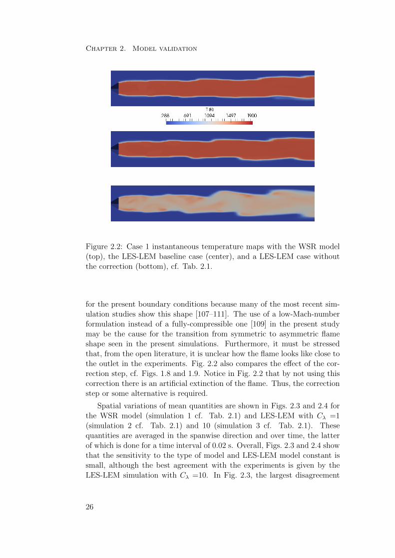
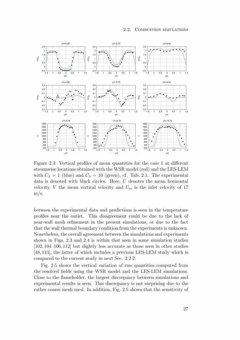
Figure 2.3: Vertical profiles of mean quantities for the case 1 at differentstreamwise locations obtained with the WSR model (red) and the LES-LEMwith Cλ = 1 (blue) and Cλ = 10 (green), cf. Tab. 2.1. The experimentaldata is denoted with black circles. Here, U denotes the mean horizontalvelocity, V the mean vertical velocity and Uin is the inlet velocity of 17m/s.

between the experimental data and predictions is seen in the temperatureprofiles near the outlet. This disagreement could be due to the lack ofnear-wall mesh refinement in the present simulations, or due to the factthat the wall thermal boundary condition from the experiments is unknown.Nonetheless, the overall agreement between the simulations and experimentsshown in Figs. 2.3 and 2.4 is within that seen in some simulation studies[102, 104–106, 112] but slightly less accurate as those seen in other studies[48, 113], the latter of which includes a previous LES-LEM study which iscompared to the current study in next Sec. 2.2.2.

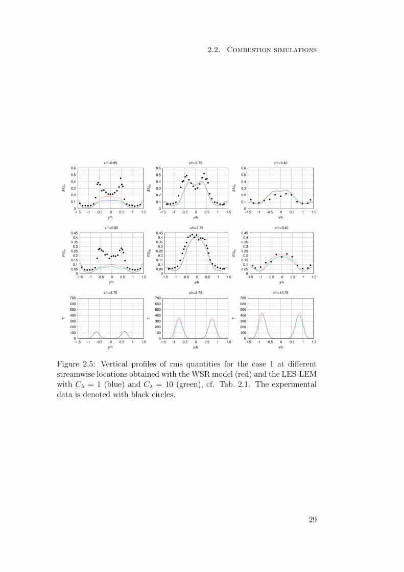
Fig. 2.5 shows the vertical variation of rms quantities computed fromthe resolved fields using the WSR model and the LES-LEM simulations.Close to the flameholder, the largest discrepancy between simulations andexperimental results is seen. This discrepancy is not surprising due to therather coarse mesh used. In addition, Fig. 2.5 shows that the sensitivity of

27


-1-0.5

0 0.5

1 1.5

2 2.5

3 3.5

4

0 2 4 6 8 10 12 14 16

U/U

in

x/h

y = 0

ExperimentsSimulation 1Simulation 2Simulation 3

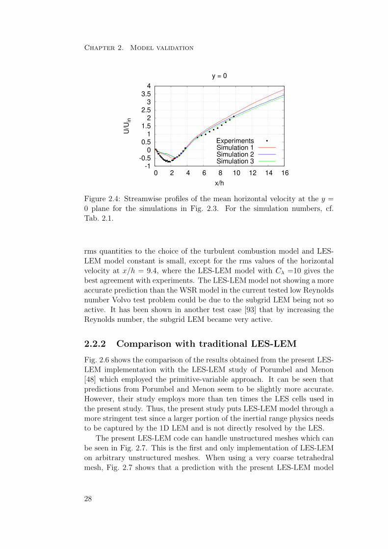
Figure 2.4: Streamwise profiles of the mean horizontal velocity at the y =0 plane for the simulations in Fig. 2.3. For the simulation numbers, cf.Tab. 2.1.

rms quantities to the choice of the turbulent combustion model and LES-LEM model constant is small, except for the rms values of the horizontalvelocity at x/h = 9.4, where the LES-LEM model with Cλ =10 gives thebest agreement with experiments. The LES-LEM model not showing a moreaccurate prediction than the WSR model in the current tested low Reynoldsnumber Volvo test problem could be due to the subgrid LEM being not soactive. It has been shown in another test case [93] that by increasing theReynolds number, the subgrid LEM became very active.

2.2.2 Comparison with traditional LES-LEM

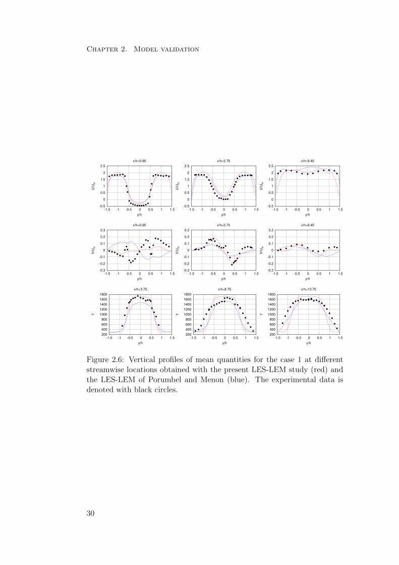
Fig. 2.6 shows the comparison of the results obtained from the present LES-LEM implementation with the LES-LEM study of Porumbel and Menon[48] which employed the primitive-variable approach. It can be seen thatpredictions from Porumbel and Menon seem to be slightly more accurate.However, their study employs more than ten times the LES cells used inthe present study. Thus, the present study puts LES-LEM model through amore stringent test since a larger portion of the inertial range physics needsto be captured by the 1D LEM and is not directly resolved by the LES.

The present LES-LEM code can handle unstructured meshes which canbe seen in Fig. 2.7. This is the first and only implementation of LES-LEMon arbitrary unstructured meshes. When using a very coarse tetrahedralmesh, Fig. 2.7 shows that a prediction with the present LES-LEM model

28


0

0.1

0.2

0.3

0.4

0.5

0.6

-1.5 -1 -0.5 0 0.5 1 1.5

U/U

in

y/h

x/h=0.95

0

0.1

0.2

0.3

0.4

0.5

0.6

-1.5 -1 -0.5 0 0.5 1 1.5

U/U

in

y/h

x/h=3.75

0

0.1

0.2

0.3

0.4

0.5

0.6

-1.5 -1 -0.5 0 0.5 1 1.5

U/U

in

y/h

x/h=9.40

0

0.05

0.1

0.15

0.2

0.25

0.3

0.35

0.4

0.45

-1.5 -1 -0.5 0 0.5 1 1.5

V/U

in

y/h

x/h=0.95

0

0.05

0.1

0.15

0.2

0.25

0.3

0.35

0.4

0.45

-1.5 -1 -0.5 0 0.5 1 1.5

V/U

in

y/h

x/h=3.75

0

0.05

0.1

0.15

0.2

0.25

0.3

0.35

0.4

0.45

-1.5 -1 -0.5 0 0.5 1 1.5

V/U

in

y/h

x/h=9.40

0

100

200

300

400

500

600

700

-1.5 -1 -0.5 0 0.5 1 1.5

T

y/h

x/h=3.75

0

100

200

300

400

500

600

700

-1.5 -1 -0.5 0 0.5 1 1.5

T

y/h

x/h=8.75

0

100

200

300

400

500

600

700

-1.5 -1 -0.5 0 0.5 1 1.5

T

y/h

x/h=13.75

Figure 2.5: Vertical profiles of rms quantities for the case 1 at differentstreamwise locations obtained with the WSR model (red) and the LES-LEMwith Cλ = 1 (blue) and Cλ = 10 (green), cf. Tab. 2.1. The experimentaldata is denoted with black circles.

29


-0.5

0

0.5

1

1.5

2

2.5

-1.5 -1 -0.5 0 0.5 1 1.5

U/U

in

y/h

x/h=0.95

-0.5

0

0.5

1

1.5

2

2.5

-1.5 -1 -0.5 0 0.5 1 1.5

U/U

in

y/h

x/h=3.75

-0.5

0

0.5

1

1.5

2

2.5

-1.5 -1 -0.5 0 0.5 1 1.5

U/U

in

y/h

x/h=9.40

-0.3

-0.2

-0.1

0

0.1

0.2

0.3

-1.5 -1 -0.5 0 0.5 1 1.5

V/U

in

y/h

x/h=0.95

-0.3

-0.2

-0.1

0

0.1

0.2

0.3

-1.5 -1 -0.5 0 0.5 1 1.5

V/U

in

y/h

x/h=3.75

-0.3

-0.2

-0.1

0

0.1

0.2

0.3

-1.5 -1 -0.5 0 0.5 1 1.5

V/U

in

y/h

x/h=9.40

200

400

600

800

1000

1200

1400

1600

1800

-1.5 -1 -0.5 0 0.5 1 1.5

T

y/h

x/h=3.75

200

400

600

800

1000

1200

1400

1600

1800

-1.5 -1 -0.5 0 0.5 1 1.5

T

y/h

x/h=8.75

200

400

600

800

1000

1200

1400

1600

1800

-1.5 -1 -0.5 0 0.5 1 1.5

T

y/h

x/h=13.75

Figure 2.6: Vertical profiles of mean quantities for the case 1 at differentstreamwise locations obtained with the present LES-LEM study (red) andthe LES-LEM of Porumbel and Menon (blue). The experimental data isdenoted with black circles.

30

2.3. Splicing investigation

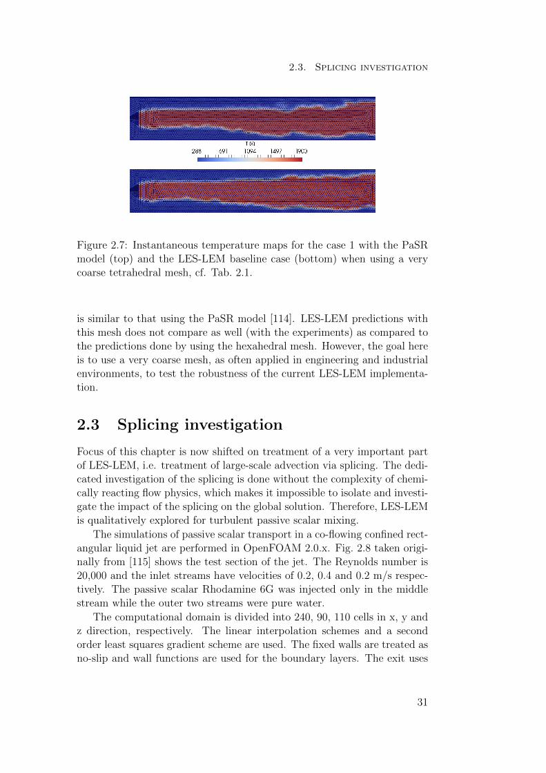
Figure 2.7: Instantaneous temperature maps for the case 1 with the PaSRmodel (top) and the LES-LEM baseline case (bottom) when using a verycoarse tetrahedral mesh, cf. Tab. 2.1.

is similar to that using the PaSR model [114]. LES-LEM predictions withthis mesh does not compare as well (with the experiments) as compared tothe predictions done by using the hexahedral mesh. However, the goal hereis to use a very coarse mesh, as often applied in engineering and industrialenvironments, to test the robustness of the current LES-LEM implementa-tion.

2.3 Splicing investigation

Focus of this chapter is now shifted on treatment of a very important partof LES-LEM, i.e. treatment of large-scale advection via splicing. The dedi-cated investigation of the splicing is done without the complexity of chemi-cally reacting flow physics, which makes it impossible to isolate and investi-gate the impact of the splicing on the global solution. Therefore, LES-LEMis qualitatively explored for turbulent passive scalar mixing.

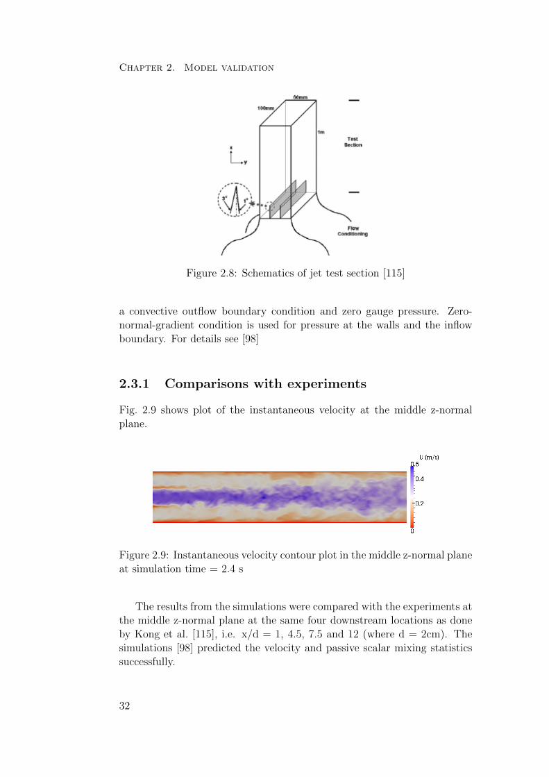
The simulations of passive scalar transport in a co-flowing confined rect-angular liquid jet are performed in OpenFOAM 2.0.x. Fig. 2.8 taken origi-nally from [115] shows the test section of the jet. The Reynolds number is20,000 and the inlet streams have velocities of 0.2, 0.4 and 0.2 m/s respec-tively. The passive scalar Rhodamine 6G was injected only in the middlestream while the outer two streams were pure water.

The computational domain is divided into 240, 90, 110 cells in x, y andz direction, respectively. The linear interpolation schemes and a secondorder least squares gradient scheme are used. The fixed walls are treated asno-slip and wall functions are used for the boundary layers. The exit uses

31


Figure 2.8: Schematics of jet test section [115]

a convective outflow boundary condition and zero gauge pressure. Zero-normal-gradient condition is used for pressure at the walls and the inflowboundary. For details see [98]

2.3.1 Comparisons with experiments

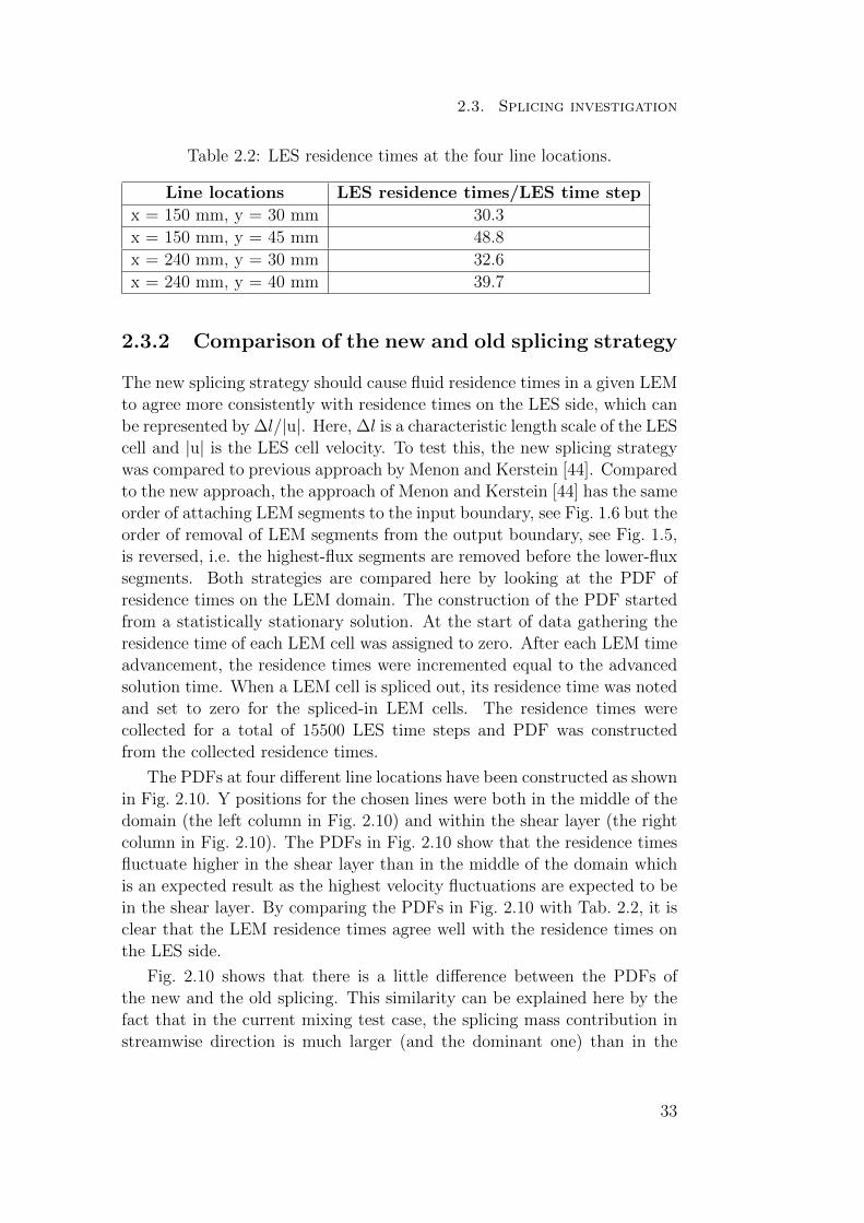
Fig. 2.9 shows plot of the instantaneous velocity at the middle z-normalplane.

Figure 2.9: Instantaneous velocity contour plot in the middle z-normal planeat simulation time = 2.4 s

The results from the simulations were compared with the experiments atthe middle z-normal plane at the same four downstream locations as doneby Kong et al. [115], i.e. x/d = 1, 4.5, 7.5 and 12 (where d = 2cm). Thesimulations [98] predicted the velocity and passive scalar mixing statisticssuccessfully.

32


Table 2.2: LES residence times at the four line locations.

Line locations LES residence times/LES time step

x = 150 mm, y = 30 mm 30.3

x = 150 mm, y = 45 mm 48.8

x = 240 mm, y = 30 mm 32.6

x = 240 mm, y = 40 mm 39.7

2.3.2 Comparison of the new and old splicing strategy

The new splicing strategy should cause fluid residence times in a given LEMto agree more consistently with residence times on the LES side, which canbe represented by ∆l/|u|. Here, ∆l is a characteristic length scale of the LEScell and |u| is the LES cell velocity. To test this, the new splicing strategywas compared to previous approach by Menon and Kerstein [44]. Comparedto the new approach, the approach of Menon and Kerstein [44] has the sameorder of attaching LEM segments to the input boundary, see Fig. 1.6 but theorder of removal of LEM segments from the output boundary, see Fig. 1.5,is reversed, i.e. the highest-flux segments are removed before the lower-fluxsegments. Both strategies are compared here by looking at the PDF ofresidence times on the LEM domain. The construction of the PDF startedfrom a statistically stationary solution. At the start of data gathering theresidence time of each LEM cell was assigned to zero. After each LEM timeadvancement, the residence times were incremented equal to the advancedsolution time. When a LEM cell is spliced out, its residence time was notedand set to zero for the spliced-in LEM cells. The residence times werecollected for a total of 15500 LES time steps and PDF was constructedfrom the collected residence times.

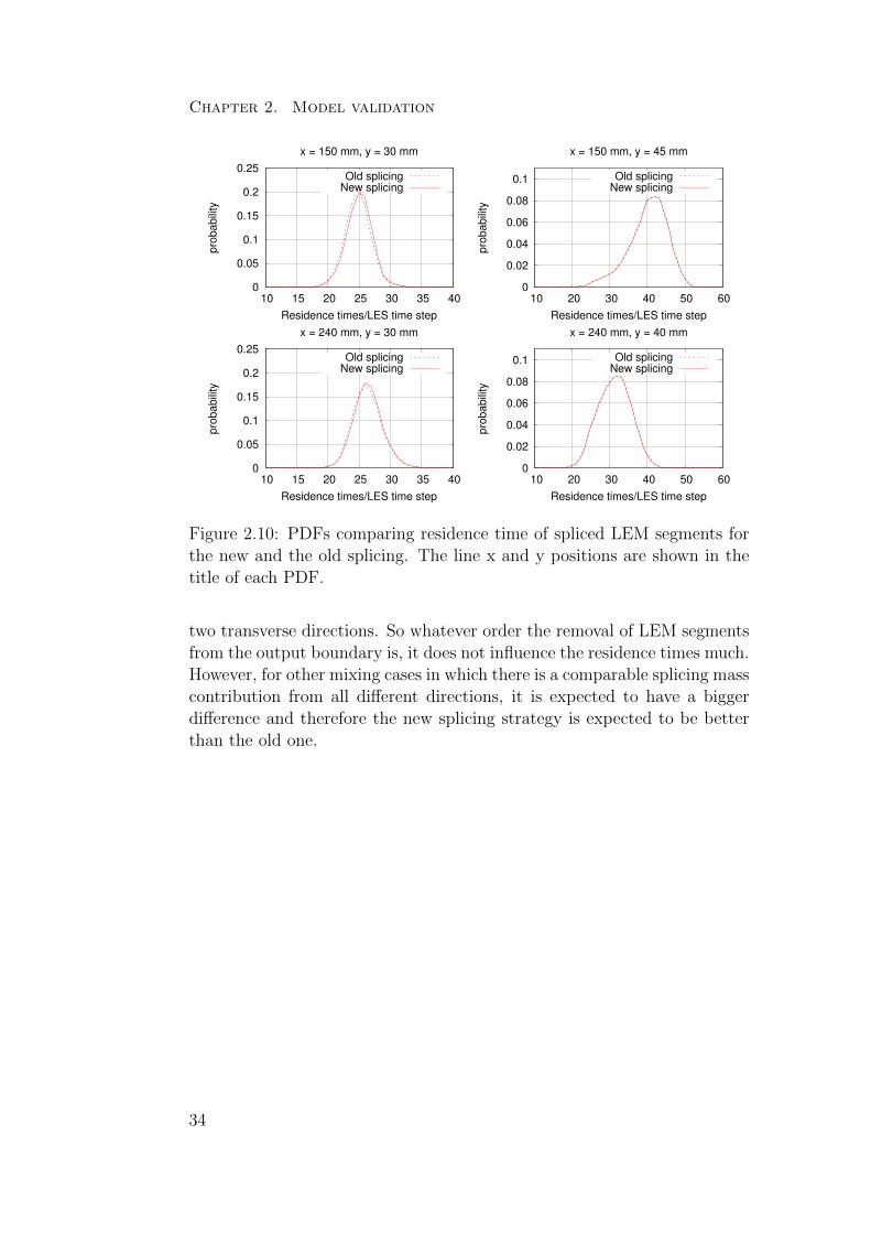
The PDFs at four different line locations have been constructed as shownin Fig. 2.10. Y positions for the chosen lines were both in the middle of thedomain (the left column in Fig. 2.10) and within the shear layer (the rightcolumn in Fig. 2.10). The PDFs in Fig. 2.10 show that the residence timesfluctuate higher in the shear layer than in the middle of the domain whichis an expected result as the highest velocity fluctuations are expected to bein the shear layer. By comparing the PDFs in Fig. 2.10 with Tab. 2.2, it isclear that the LEM residence times agree well with the residence times onthe LES side.

Fig. 2.10 shows that there is a little difference between the PDFs ofthe new and the old splicing. This similarity can be explained here by thefact that in the current mixing test case, the splicing mass contribution instreamwise direction is much larger (and the dominant one) than in the

33


Figure 2.10: PDFs comparing residence time of spliced LEM segments forthe new and the old splicing. The line x and y positions are shown in thetitle of each PDF.

two transverse directions. So whatever order the removal of LEM segmentsfrom the output boundary is, it does not influence the residence times much.However, for other mixing cases in which there is a comparable splicing masscontribution from all different directions, it is expected to have a biggerdifference and therefore the new splicing strategy is expected to be betterthan the old one.

34

Conclusion

The main contributions of this thesis are:

• Implementation of LES-LEM in a pressure-based and unstructuredgrid solver in OpenFOAM.

• Development and implementation of a new LEM closure for LES withthe reaction-rate approach. LES-LEM model with the new LEM clo-sure was tested on the premixed Volvo combustor and the predictionswere found to be within those of previous simulations.

• Development and implementation of a new splicing strategy based onan ordered flux of spliced LEM segments. The new splicing strategywas tested by simulating passive scalar mixing. The simulation resultswere compared to experiments and it was shown that the simulationscorrectly predict velocity statistics and passive scalar mixing. It wasshown that the splicing represents large-scale advection in LES-LEMreasonably well, which has been implicitly assumed in combustionLES-LEM but never demonstrated in an isolated setting.

• Development and implementation of the super-grid LES-LEM. Firstdemonstration of the expected computational speed-up compared tostandard LES-LEM.

35

Future work

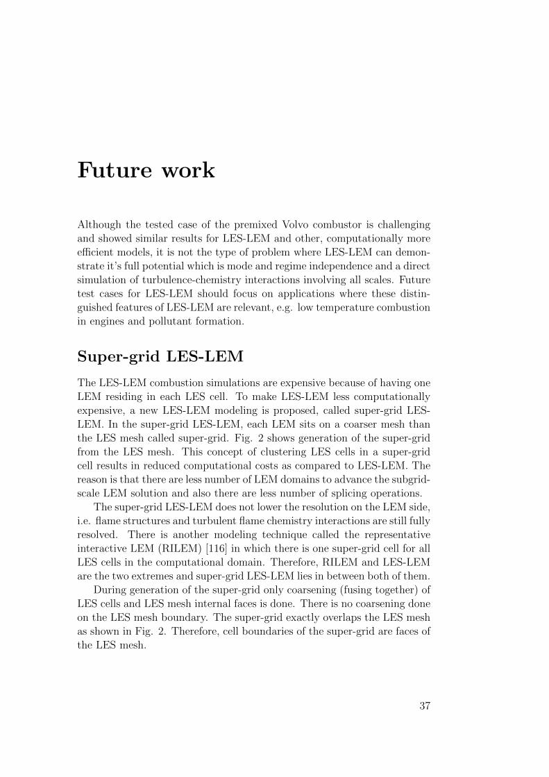
Although the tested case of the premixed Volvo combustor is challengingand showed similar results for LES-LEM and other, computationally moreefficient models, it is not the type of problem where LES-LEM can demon-strate it’s full potential which is mode and regime independence and a directsimulation of turbulence-chemistry interactions involving all scales. Futuretest cases for LES-LEM should focus on applications where these distin-guished features of LES-LEM are relevant, e.g. low temperature combustionin engines and pollutant formation.

Super-grid LES-LEM

The LES-LEM combustion simulations are expensive because of having oneLEM residing in each LES cell. To make LES-LEM less computationallyexpensive, a new LES-LEM modeling is proposed, called super-grid LES-LEM. In the super-grid LES-LEM, each LEM sits on a coarser mesh thanthe LES mesh called super-grid. Fig. 2 shows generation of the super-gridfrom the LES mesh. This concept of clustering LES cells in a super-gridcell results in reduced computational costs as compared to LES-LEM. Thereason is that there are less number of LEM domains to advance the subgrid-scale LEM solution and also there are less number of splicing operations.

The super-grid LES-LEM does not lower the resolution on the LEM side,i.e. flame structures and turbulent flame chemistry interactions are still fullyresolved. There is another modeling technique called the representativeinteractive LEM (RILEM) [116] in which there is one super-grid cell for allLES cells in the computational domain. Therefore, RILEM and LES-LEMare the two extremes and super-grid LES-LEM lies in between both of them.

During generation of the super-grid only coarsening (fusing together) ofLES cells and LES mesh internal faces is done. There is no coarsening doneon the LES mesh boundary. The super-grid exactly overlaps the LES meshas shown in Fig. 2. Therefore, cell boundaries of the super-grid are faces ofthe LES mesh.

37


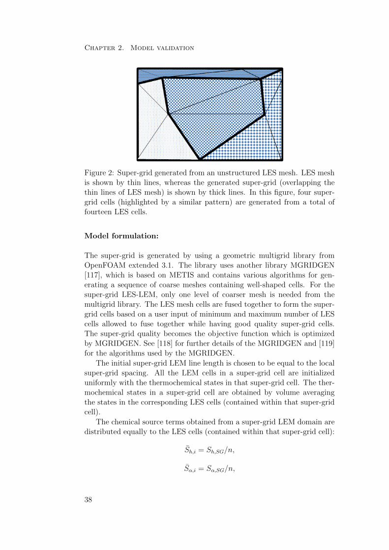
Figure 2: Super-grid generated from an unstructured LES mesh. LES meshis shown by thin lines, whereas the generated super-grid (overlapping thethin lines of LES mesh) is shown by thick lines. In this figure, four super-grid cells (highlighted by a similar pattern) are generated from a total offourteen LES cells.

Model formulation:

The super-grid is generated by using a geometric multigrid library fromOpenFOAM extended 3.1. The library uses another library MGRIDGEN[117], which is based on METIS and contains various algorithms for gen-erating a sequence of coarse meshes containing well-shaped cells. For thesuper-grid LES-LEM, only one level of coarser mesh is needed from themultigrid library. The LES mesh cells are fused together to form the super-grid cells based on a user input of minimum and maximum number of LEScells allowed to fuse together while having good quality super-grid cells.The super-grid quality becomes the objective function which is optimizedby MGRIDGEN. See [118] for further details of the MGRIDGEN and [119]for the algorithms used by the MGRIDGEN.

The initial super-grid LEM line length is chosen to be equal to the localsuper-grid spacing. All the LEM cells in a super-grid cell are initializeduniformly with the thermochemical states in that super-grid cell. The ther-mochemical states in a super-grid cell are obtained by volume averagingthe states in the corresponding LES cells (contained within that super-gridcell).

The chemical source terms obtained from a super-grid LEM domain aredistributed equally to the LES cells (contained within that super-grid cell):

Sh,i = Sh,SG/n,

Sα,i = Sα,SG/n,

38


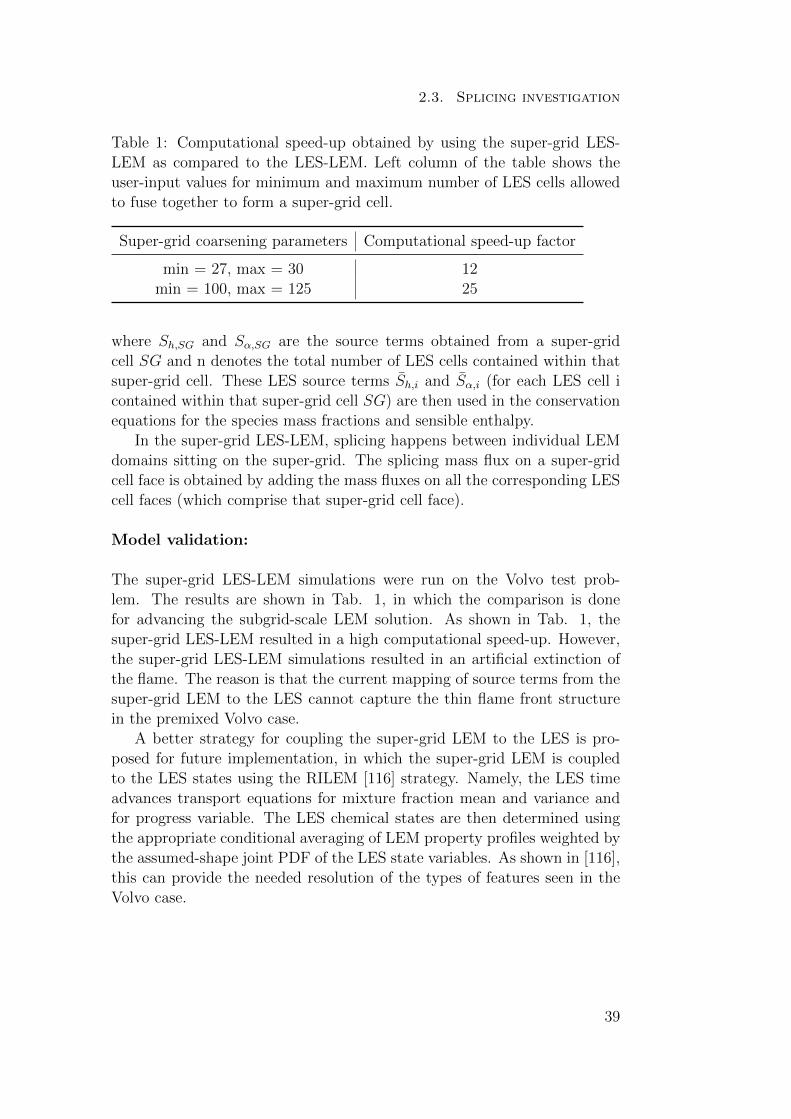
Table 1: Computational speed-up obtained by using the super-grid LES-LEM as compared to the LES-LEM. Left column of the table shows theuser-input values for minimum and maximum number of LES cells allowedto fuse together to form a super-grid cell.

Super-grid coarsening parameters Computational speed-up factor

min = 27, max = 30 12min = 100, max = 125 25

where Sh,SG and Sα,SG are the source terms obtained from a super-gridcell SG and n denotes the total number of LES cells contained within thatsuper-grid cell. These LES source terms Sh,i and Sα,i (for each LES cell icontained within that super-grid cell SG) are then used in the conservationequations for the species mass fractions and sensible enthalpy.

In the super-grid LES-LEM, splicing happens between individual LEMdomains sitting on the super-grid. The splicing mass flux on a super-gridcell face is obtained by adding the mass fluxes on all the corresponding LEScell faces (which comprise that super-grid cell face).

Model validation:

The super-grid LES-LEM simulations were run on the Volvo test prob-lem. The results are shown in Tab. 1, in which the comparison is donefor advancing the subgrid-scale LEM solution. As shown in Tab. 1, thesuper-grid LES-LEM resulted in a high computational speed-up. However,the super-grid LES-LEM simulations resulted in an artificial extinction ofthe flame. The reason is that the current mapping of source terms from thesuper-grid LEM to the LES cannot capture the thin flame front structurein the premixed Volvo case.

A better strategy for coupling the super-grid LEM to the LES is pro-posed for future implementation, in which the super-grid LEM is coupledto the LES states using the RILEM [116] strategy. Namely, the LES timeadvances transport equations for mixture fraction mean and variance andfor progress variable. The LES chemical states are then determined usingthe appropriate conditional averaging of LEM property profiles weighted bythe assumed-shape joint PDF of the LES state variables. As shown in [116],this can provide the needed resolution of the types of features seen in theVolvo case.

39

Summary of papers

Paper 1

Effect of the turbulence modeling in large-eddy simulations ofnonpremixed flames undergoing extinction and reignition

In this paper the effect of three turbulent combustion models, i.e. no-model,PaSR and LEM was studied for a flame with extinction and reignition.Two levels of mesh refinement and two eddy-viscosity models were usedand two types of temporal jets were considered and their DNS results werequalitatively compared with LES results. It was found that LES capturesqualitatively the extinction and reignition observed in the DNS simulations.The sensitivity to the turbulent combustion model was not negligible andthe PaSR model showed the best accuracy. I implemented the LES-LEMmodel and ran the simulations together with Adhiraj Dasgupta. EstebanD. Gonzalez wrote the paper with support from me and Adhiraj Dasguptawho performed post-processing. Michael Oevermann provided supervisionof the work.

Paper 2

Turbulent-combustion closure for the chemical source terms usingthe linear-eddy model

A new method to use LEM to close the filtered chemical source terms inthe conservation equations of the thermochemical quantities is tested on abluff-body stabilized flame case. The predictions using this closure werefound to agree with experimental data within the same range of accuracyas the previous simulations. I implemented the new LEM closure for theLES-LEM model and improved the model from Paper 1 by further imple-mentations. I assisted Esteban D. Gonzalez in the writing, by writing partsof the paper. Simulations were run by both me and Esteban D. Gonzalez.

41


This work was performed under guidance of Michael Oevermann and SureshMenon.

Paper 3

A strategy for large-scale scalar advection in large eddy simula-tions that use the linear eddy sub-grid mixing model

A new strategy for splicing is implemented in a pressure-based fluid solverand tested by simulation of passive scalar transport in a co-flowing turbu-lent rectangular jet using unstructured grids. The simulation results showedgood agreement with the experiments. This dedicated investigation of splic-ing concluded that the new splicing strategy represents large-scale advectionin LES-LEM in a reasonable way. The new splicing strategy was proposedby Alan Kerstein and Michael Oevermann and Bo Kong provided the experi-mental data and simulation setup of the case. I implemented LES-LEM withthe new splicing strategy, performed all the simulations, post-processed andanalyzed the results. I wrote the paper with input from all the co-authorsand presented it at the International Conference on Computational Heatand Mass Transfer held in Krakow in May 2016. The paper was chosenfor publication as a Journal article in International Journal of NumericalMethods for Heat and Fluid Flow.

Paper 4

Subgrid reaction-diffusion closure for large eddy simulations usingthe linear-eddy model

In this paper a more detailed evaluation of the reaction-rate approach pre-sented in paper 2 is done and more simulations were performed including anon-premixed syngas flame. After several months of simulating, post pro-cessing and analysis of the results I wrote this paper with input from allco-authors. The paper has been accepted for publication in Flow, Turbu-lence and Combustion.

42

References

[1] Kerstein, A.R.: Linear eddy modeling of turbulent transport and mix-ing. Combust. Sci. Technol. 60, 391-421 (1988)

[2] Peters, N.: Turbulent combustion. Cambridge Uni. Press (2000).

[3] Poinsot, T., Veynante, D.: Theoretical and Numerical Combustion. R.T. Edwards, Inc., Philadelphia (2005)

[4] Gonzalez-Juez, E.D., Kerstein, A.R., Ranjan, R., Menon, S.: Advancesand challenges in modeling high-speed turbulent combustion in propul-sion systems. Progr. Energy Combust. Sci. 60, 26-67 (2017)

[5] Oefelein, J.C.: Analysis of turbulent combustion modeling approachesfor aero-propulsion applications. AIAA paper 2015-1378 (2015)

[6] Fureby, C.: A comparative study of large eddy simulation (LES) com-bustion models applied to the volvo validation rig. AIAA paper 2017-1575 (2017)

[7] Pitsch, H.: Large-Eddy simulation of turbulent combustion. AnnualReview Fluid Mech. 38(4), 453-482 (2006)

[8] http://personalpages.to.infn.it/ fre/RTIgnitor/pdfversie/Petrosyan2.pdf

[9] Jhavar, R. and Rutland, C.J.: Using Large Eddy Simulations to StudyMixing Effects in Early Injection Diesel Engine Combustion. SAETechn. Paper 2006-01-0871 (2006)

[10] Adomeit, P., Lang, O., Pischinger, S., Aymanns, R., Graf, M., Stapf,G.: Analysis of Cyclic Fluctuations of Charge Motion and MixtureFormation in a DISI Engine in Stratified Operation. SAE Techn. Paper2007-01-1412 (2007)

[11] Yu, R., Bai, X.S., Hildingsson, L., Hultqvist, A., Miles, P.C.: Nu-merical and Experimental Investigation of Turbulent Flows in a DieselEngine. SAE Techn. Paper 2006-01-3436 (2006)

43

References

[12] Yu, R., Bai, X.S., Vressner, A., Hultqvist, A., Johansson, B., Olofsson,J., Seyfried, H., Sjoholm, J., Richter, M., Alden, M.: Effect of Turbu-lence on HCCI Combustion. SAE Techn. Paper 2007-01-0183 (2007)

[13] Joelsson, T., Yu, R., Bai, X.S., Vressner, A., Johansson, B.: LargeEddy Simulation and Experiments of the Auto-Ignition Process of LeanEthanol/Air Mixture in HCCI Engines. SAE Int. J. Fuels Lubricants1(1), 1110-1119 (2008)

[14] Rutland, C. J.: Large-eddy simulations for internal combustion engines- a review. Int. J. Engine Res. 12(5), 421-451 (2011)

[15] Kosters, A., Golovitchev, V., Karlsson, A.: SAE, Int. J. Fuels Lubr.,5:604-610 (2012)

[16] Kosters, A., Karlsson, A., Oevermann, M., D’Errico, G., Lucchini, T.:Combust. Theory Model., 19:81-106 (2015)

[17] D’Errico, G., Lucchini, T., Contino, F., Jangi, M., Bai, X.S.: Combust.Theory Model., 18:65-88 (2014)

[18] Kong, S.C., Reitz, R.D.: J. Eng. Gas Turb. Power, 124:702-707 (2002)

[19] Kokjohn, S., Hanson, R.M., Splitter, D.A., Reitz, R.D.: SAE TechnicalPaper, 2009-01-2647 (2009)

[20] Knudsen, E., Kim, S.H., Pitsch, H.: Phys. Fluids, 22, 115109 (2010)

[21] Mittal, V., Pitsch, H.: Proc. Combust. Inst., 34:2995-3003 (2013)

[22] Peters, N.: Prog. Energy Combust. Sci., 10:319-339 (1984)

[23] Ihme, M., Pitsch, H.: Combust. Flame, 155:70-89 (2008)

[24] Nguyen, P., Vervisch, L., Subramanian, V., Domingo, P.: Combust.Flame, 157:43-61 (2010)

[25] Knudsen, E., Pitsch, H.: Combust. Flame, 159:242-264 (2012)

[26] Knudsen, E., Pitsch, H.: Combust. Flame, 156:678-696 (2009)

[27] Pitsch, H., Fedotov, S.: Combust. Theory, Model., 5:41-57 (2001)

[28] Pitsch, H., Cha, C.M., Fedotov, S.: Combust. Theory Model., 7:317-332 (2003)

[29] Lucchini, T., D’Errico, G., Onorati, A., Frassoldati, A., Stagni, A.,Hardy, G.: SAE Int. J. Engines, 10:2017 (2017)

44

References

[30] Barths, H., Hasse, C., Bikas, G., Peters, N.: Proc. Combust. Inst.,28:1161-1168 (2000)

[31] Barths, H., Antoni, C., Peters, N.: SAE Technical Paper, 982459 (1998)

[32] Hasse, C., Barths, H., Peters, N.: SAE Technical Paper, 1999-01-3547(1999)

[33] Hergarth, C., Barths, H., Peters, N.: SAE Technical Paper, 1999-01-3550 (1999)

[34] Pitsch, H., Wan, H., Peters, N.: SAE Technical Paper, 952357 (1995)

[35] Pitsch, H., Barths, H., Peters, N.: SAE Technical Paper, 962057 (1996)

[36] Maghbouli, A., Lucchini, T., D’Errico, G., Onorati, A., Malbec, L.M., Musculus, M., Eagle, W.E.: SAE Technical Paper, 2016-01-0577(2016)

[37] Klimenko, A.Y., Bilger, R.W.: Prog. Energy Combust. Sci., 25:595-688(1999)

[38] Paola, G. De, Mastorakos, E., Wright, Y. M., Boulouchos, K.: Comb.Sci. Tech., 180:883-899 (2008)

[39] Bolla, M., Farrace, D., Wright, Y.M., Boulouchos, K.: Fuel, 117:309-325 (2014)

[40] Pope, S.B.: Annu. Rev. Fluid, Mech., 26:23-63 (1994)

[41] Zhang, Y.Z., Kung, E.H., Haworth, D.C.: Proc. Combust. Inst.,30:2763-2771 (2005)

[42] Mohan, V.R., Haworth, D.C.: Proc. Combust. Inst., 3053-3060 (2015)

[43] Menon, S., Kerstein, A.R., McMurtry, P.A.: A linear eddy mixingmodel for large eddy simulation of turbulent combustion. In: LargeEddy Simul. Complex Eng. Geophysical Flows, Galperin, B., Orszag,S.A., pp. 287-314. Cambridge University Press (1993)

[44] Menon, S., Kerstein, A.R.: The Linear-Eddy Model. In: Turbu-lent Combustion Modeling, Echekki, T., Mastorakos, E., pp. 221-247.Springer Series, Vol. 95, New York (2011)

[45] Kerstein, A.R.: Linear-eddy modelling of turbulent transport. Part 7.Finite-rate chemistry and multi-stream mixing. J. Fluid Mech. 240,289-313 (1992)

45

References

[46] Menon, S., Sankaran, V., Stone, C.: Subgrid combustion modelingfor the next generation National Combustion Code. NASA Tech. Rep.2003-212202 (2003)

[47] Sankaran, V.: Subgrid combustion modeling for compressible two-phase reacting flow. Ph.D. thesis, Georgia Institute of Technology(2003)

[48] Porumbel, I., Menon, S.: Large eddy simulation of bluff body stabilizedpremixed flame. AIAA Paper 2006-152 (2006)

[49] Parisi, V.: Large Eddy Simulation of a Non-Premixed Stagnation PointReverse Flow Combustor. Master’s thesis, Georgia Institute of Tech-nology (2006)

[50] Undapalli, S.: Large eddy simulation of premixed and non-premixedcombustion in a stagnation point reverse flow combustor. Ph.D. thesis,Georgia Institute of Technology (2008)

[51] Sen, B.A., Menon, S.: Artificial neural networks based chemistry-mixing subgrid model for LES. AIAA Paper 2009-241 (2009)

[52] Genin, F., Menon, S.: Simulation of turbulent mixing behind a strutinjector in supersonic flow. AIAA Paper 2009-132 (2009)

[53] Wey, T., Liu, N.: Assessment of turbulence-chemistry interaction mod-els in the National Combustion Code (NCC) - Part I. AIAA Paper2010-16098 (2010)

[54] Liu, N., Wey, T.: On the TFNS Subgrid Models for Liquid-FueledTurbulent Combustion. AIAA Paper 2014-3569 (2014)

[55] Harvazinski, M.E., Huang, C., Sankaran, V., Feldman, T.W., Ander-son, W.E., Merkle, C.L., Talley, D.G.: Coupling between hydrodynam-ics, acoustics, and heat release in a self-excited unstable combustor.Phys. Fluids 27, No. 4, 045102 (2015)

[56] Fureby, C., Zettervall, N., Kim, S., Menon, S.: Large eddy simulation ofa simplified lean premixed gas turbine combustor. Intl. Symp. Turbul.Shear Flow Phenom. (2015)

[57] Maxwell, B.M., Falle, S.A.E.G., Sharpe, G., Radulescu, M.I.: Acompressible-LEM turbulent combustion subgrid model for assessinggaseous explosion hazards. J. Loss Prevention Process Industries 36,460-470 (2015)

46

References

[58] Li, S., Zheng, Y., Mira, D., Li, S., Zhu, M., Jiang, X.: A LES-LEMstudy of preferential diffusion processes in a partially premixed swirlingcombustor with synthesis gases. J. Eng. Gas Turbine Power 139, 031501(2016)

[59] McMurtry, P.A., Menon, S., Kerstein, A.R.: A linear eddy sub-gridmodel for turbulent reacting flows: Application to hydrogen-AIR com-bustion. Proc. Combust. Inst. 24, 271-278 (1992)

[60] Calhoon, W.H.: On subgrid combustion modeling for large-eddy sim-ulations. PhD thesis, Georgia Institute of Technology (1996)

[61] Menon, S., Calhoon, W.H.: Subgrid mixing and molecular transportmodeling in a reacting shear layer. Proc. Combust. Inst. 26, 59-66,(1996)

[62] Smith, T.M.: Unsteady simulations of turbulent premixed reactingflows. PhD thesis, Georgia Institute of Technology (1998)

[63] Chakravarthy, V.K., Menon, S.: Subgrid modeling of turbulent pre-mixed flames in the flamelet regime. Flow, Turbul. Combust. 65, 133-161 (2000)

[64] Pannala, S., Menon, S.: Large eddy simulations of two-phase turbulentflows. AIAA Paper 1998-0163 (1998)

[65] Zimberg, M.J., Frankel, S.H., Gore, J.P., Sivathanu, Y.R.: A study ofcoupled turbulent mixing, soot chemistry, and radiation effects usingthe linear eddy model. Combust. Flame 113, 454-469 (1998)

[66] Sankaran, V., Menon, S.: Subgrid combustion modeling of 3-D pre-mixed flames in the thin-reaction-zone regime. Proc. Combust. Inst.30, 575-582 (2005)

[67] Sen, B.A., Menon, S.: Linear eddy mixing based tabulation and arti-ficial neural networks for large eddy simulations of turbulent flames.Combust. Flame 157, 62-74 (2010)

[68] Sen, B.A., Hawkes, E.R., Menon, S.: Large eddy simulation of ex-tinction and reignition with artificial neural networks based chemicalkinetics. Combust. Flame 157, 566-578 (2010)

[69] Ochoa, J.S., Sanchez-Insa, A., Fueyo, N.: Subgrid linear eddy mixingand combustion modelling of a turbulent nonpremixed piloted jet flame.Flow, Turbul. Combust. 89, 295-309 (2012)

47

References

[70] Choi, J.J., Menon, S.: Large eddy simulation of cavity-stabilized su-personic combustion. AIAA Paper 2009-5383 (2009)

[71] Sone, K., Menon, S.: Effect of subgrid modeling on the in-cylinder un-steady mixing process in a direct injection engine. J. Eng. Gas TurbinesPower 125(2), 435-443 (2003)

[72] Steeper, R., Sankaran, V., Oefelein, J., Hessel, R.: Simulation of theeffect of spatial fuel distribution using a linear-eddy model. SAE Tech-nical Paper 2007-01-4131 (2007)

[73] Martinez, D.M., Jiang, X., Moulinec, C., Emerson, D.R.: Numericalsimulations of turbulent jet flames with non-premixed combustion ofhydrogen-enriched fuels. Comput. & Fluids 88, 688-701 (2013)

[74] Martinez, D.M., Jiang, X., Moulinec, C., Emerson, D.R.: Numericalassessment of subgrid scale models for scalar transport in large-eddysimulations of hydrogen-enriched fuels. Int. J. Hydrogen Energy 39,7173-7189 (2014)

[75] Lovett, J.A., Ahmed, K., Bibik, O., Smith, A.G., Lubarsky, E., Menon,S., Zinn, B.T.: On the influence of fuel distribution on the flame struc-ture of bluff-body stabilized flames. J. Eng. Gas Turbines Power 136(4),041503 (2013)

[76] Srinivasan, S., Ranjan, R., Menon, S.: Flame dynamics during com-bustion instability in a high-pressure, shear-coaxial injector combustor.Flow, Turbul. Combust. 94, 237-262 (2015)

[77] Srinivasan, S., Kozaka, E.O., Menon, S.: A new subgrid breakup modelfor LES of spray mixing and combustion. In: Direct and Large-EddySimulation VIII, pp. 333-338. ERCOFTAC, Springer Science and Busi-ness Media (2011)

[78] Pope, S.B.: PDF methods for turbulent reactive flows. Prog. EnergyCombust. Sci. 11, No. 2, 119-192 (1985)

[79] Haworth, D.C.: Progress in probability density function methods forturbulent reacting flows. Prog. Energy Combust. Sci. 36, No. 2, 168-259(2010)

[80] Haworth, D.C., Pope, S.B.: Transported probability density functionmethods for Reynolds-averaged and large-eddy simulations. TurbulentCombust. Model., 119-142 (2011)

48

References

[81] Pope, S.B.: Small scales, many species and the manifold challenges ofturbulent combustion. Proc. Combust. Inst. 34, No. 1, 1-31 (2013)

[82] Wu, H., See, Y.C., Wang, Q., Ihme, M.: A pareto-efficient combustionframework with submodel assignment for predicting complex flame con-figurations. Combust. Flame 162, No. 11, 4208-4230 (2015)

[83] Gada, V.H., Tandon, M.P., Elias, J., Vikulov, R., Lo, S.: A largescale interface multi-fluid model for simulating multiphase flows. Appl.Math. Model. 44, 189-204 (2017)

[84] OpenFOAM, software available at http://www.openfoam.org.

[85] Weller, H.G., Tabor, G., Jasak, H., Fureby, C.: A tensorial approach tocomputational continuum mechanics using object-oriented techniques.Comput. Phys. 12, No. 6, 620-631 (1998)

[86] Yoshizawa, A., Horiuti, K.: A statistically-derived subgrid-scale kineticenergy model for the large eddy simulation of turbulent flows. J. Phys.Soc. Japan 54, 2834-2839 (1985)

[87] Gonzalez-Juez, E.D., Dasgupta, A., Arshad, S., Oevermann, M.,Lignell, D.: Effect of the turbulence modeling in large-eddy simulationsof nonpremixed flames undergoing extinction and reignition. AIAA Pa-per 2017-0604 (2017)

[88] Kerstein, A.R.: One-dimensional turbulence: model formulation andapplication to homogeneous turbulence, shear flows, and buoyant strat-ified flows. J. Fluid Mech. 392, 277-334 (1999)

[89] Grøvdal, F.: A dimensional-decomposition approach for stochasticscale-resolving simulations of turbulent reacting flows. Ph.D. thesis,Norwegian University of Science and Technology (2018)

[90] Richardson, L.F.: Weather Prediction by Numerical Process. Republi-cation. Dover Publ., New York 1965. (Cambridge Univ. Press, London)(1922)

[91] Richardson, L.F.: Atmospheric diffusion shown on a distance-neighbour graph. Proceedings of the Royal Society of London. Se-ries A, Containing Papers of a Mathematical and Physical Character,110(756):709-737 (1926)

[92] Issa, R.I.: Solution of the implicitly discretised fluid flow equations byoperator-splitting. J. Comput. Phys. 62, No. 1, 40-65 (1986)

49

References

[93] Arshad, S., Gonzalez-Juez, E.D., Dasgupta, A., Menon, S., Oever-mann, M.: Subgrid reaction-diffusion closure for large eddy simulationsusing the linear-eddy model. Flow, Turbul. Combust. submitted (2018)

[94] Sjunnesson, A., Nelson, C., Max, E.: LDA Measurements of velocitiesand turbulence in a bluff body stabilized flame. Proc. 4th Intl. Conf.Laser Anemometry, Cleveland, OH (1991)

[95] Sjunnesson, A., Olovsson, S., Sjoblom, B.: Validation rig – A tool forflame studies. Volvo Flygmotor Intern. Rep. VFA 9370-308 (1991)

[96] Sjunnesson, A., Henrikson, P., Lofstrom, C.: CARS measurements andvisualization of reacting flows in a bluff body stabilized flame. AIAAPaper 1992-3650 (1992)

[97] Ma, F., Proscia, W., Ivanov, V., Montanari, F.: Large eddy simulationof self-excited combustion dynamics in a bluff-body combustor. AIAAPaper 2015-3968 (2015)

[98] Arshad, S., Kong, B., Kerstein, A.R., Oevermann, M.: A strategy forlarge-scale scalar advection in large eddy simulations that use the lineareddy sub-grid mixing model. Intl. J. Numer. Methods Heat Fluid Flow,in press (2018)

[99] Duwig, C., Nogenmyr, K., Chan, C., Dunn, M.J.: Large eddy simu-lations of a piloted lean premix jet flame using finite-rate chemistry.Combust. Theory Model. 15, No. 4, 537-568 (2011)

[100] Fiorina, B., Mercier, R., Kuenne, G., Ketelheun, A., Avdic, A., Jan-icka, J., Geyer, D., Dreizler, A., Alenius, E., Duwig et al. C.: Challeng-ing modeling strategies for LES of non-adiabatic turbulent stratifiedcombustion. Combust. Flame 162, No. 11, 4264-4282 (2015)

[101] Moller, S., Lundgren, E., Fureby, C.: Large eddy simulation of un-steady combustion. Int. Symposium Combust. 26, No. 1, 241-248 (1996)

[102] Fureby, C.: Large eddy simulation of combustion instabilities in a jetengine afterburner model. Combust. Sci. Technol. 161, No.1, 213-243(2000)

[103] Comer, A.L., Huang, C., Rankin, B.A., Harvazinski, M.E., Sankaran,V.: Modeling and simulation of bluff body stabilized turbulent pre-mixed flames. AIAA Paper 2016-1936 (2016)

50

References

[104] Giacomazzi, E., Battaglia, V., Bruno, C.: The coupling of turbulenceand chemistry in a premixed bluff-body flame as studied by LES. Com-bust. Flame 138, No. 4, 320-335 (2004)

[105] Cocks, P.A.T., Soteriou, M.C., Sankaran, V.: Impact of numerics onthe predictive capabilities of reacting flow LES. Combust. Flame 162,No. 9, 3394-3411 (2015)

[106] Baudoin, E., Nogenmyr, K.J., Bai, X.S., Fureby, C.: Comparisonof LES models applied to a bluff body stabilized flame. AIAA Paper2009-1178 (2009)

[107] Fureby, C.: A comparative study of large eddy simulation (LES) com-bustion models applied to the Volvo validation rig. AIAA Paper 2017-1575 (2017)

[108] Drennan, S.A., Kumar, G., Liu, S.: Developing grid-convergent LESsimulations of augmentor combustion with automatic meshing andadaptive mesh refinement. AIAA Paper 2017-1574 (2017)

[109] Gonzalez-Juez, E.D.: Numerical simulations of thermoacoustic com-bustion instabilities in the Volvo combustor. AIAA Paper 2017-4686(2017)

[110] Wu, H., Ma, P.C., Lv, Y., Ihme, M.: MVP-workshop contribution:Modeling of Volvo bluff body flame experiment. AIAA Paper 2017-1573(2017)

[111] Sankaran, V., Gallagher, T.: Grid convergence in LES of bluff bodystabilized flames. AIAA Paper 2017-1791 (2017)

[112] Durand, L., Polifke, W.: Implementation of the thickened flame modelfor large eddy simulation of turbulent premixed combustion in a com-mercial solver. ASME Paper GT2007-281888 (2007)

[113] Jones, W.P., Marquis, A.J., Wang, F.: Large eddy simulation of a pre-mixed propane turbulent bluff body flame using the Eulerian stochasticfield method. Fuel 140, 514-525 (2015)

[114] Nordin, P.A.N.: Complex chemistry modeling of diesel spray combus-tion. Ph.D. thesis, Chalmers University of Technology (2001)

[115] Kong, B., Olsen, M. G., Fox, R. O., Hill, J. C.: Predictive capability ofLarge Eddy Simulation for point-wise and spatial turbulence statisticsin a confined rectangular jet. Chem. Engineering Sci. 69, 240-256 (2012)

51

References

[116] Lackmann, T.: A representative interactive linear-eddy-model(RILEM) for simulating spray combustion. Ph.D. thesis, Chalmers Uni-versity of Technology (2017)

[117] Available at http://www-users.cs.umn.edu/ moulitsa/software.html

[118] Available at http://www-users.cs.umn.edu/ moulitsa/download/manual-parmgridgen.pdf

[119] Moulitsas, I., Karypis, G.: Multilevel algorithms for generating coarsegrids for multigrid methods. Supercomputing Conf. Proc. (2001)

52

Large eddy simulation of combustion using linear-eddy ... · Large eddy simulation of combustion...

Documents

Transcript of Large eddy simulation of combustion using linear-eddy ... · Large eddy simulation of combustion...