CONFIDENTIAL Antonius Pieter van Gurp Repository version ...
94
DEVELOPMENT OF A PLOUGH PULLING FORCE MODEL FOR SUBMARINE NARROW SHAPED PLOUGHS CONFIDENTIAL Antonius Pieter van Gurp Repository version – October 8, 2014 Delft University of Technology Section of Dredging Engineering
Transcript of CONFIDENTIAL Antonius Pieter van Gurp Repository version ...
DEVELOPMENT OF A PLOUGH PULLING FORCE MODEL FOR SUBMARINE
NARROW SHAPED PLOUGHS
CONFIDENTIAL
Antonius Pieter van Gurp
Repository version – October 8, 2014
Delft University of Technology
Section of Dredging Engineering

i
DEVELOPMENT OF A PLOUGH PULLING FORCE MODEL FOR SUBMARINE
NARROW SHAPED PLOUGHS
Author:
A.P. van Gurp
Thesis Committee:
Prof. dr. ir. C. van Rhee Delft University of Technology
Dr. ir. S.A. Miedema Delft University of Technology
Dr. ir. D.J.M. Ngan-Tillard Delft University of Technology
Ir. L. van Baalen VolkerWessels Boskalis Marine Solutions
Ing. M. Biesheuvel Koninklijke Boskalis Westminster N.V.
Under the authority of:
Delft University of Technology
VolkerWessels Boskalis Marine Solutions
Koninklijke Boskalis Westminster N.V.

ii
iii
ABSTRACT
Development of a plough pulling force model for submarine narrow
shaped ploughs
Antonius Pieter van Gurp
Delft University of Technology, 2014
iv
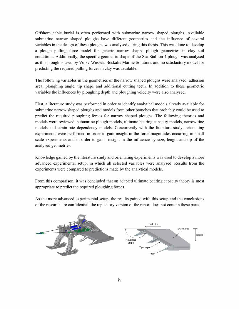
Offshore cable burial is often performed with submarine narrow shaped ploughs. Available
submarine narrow shaped ploughs have different geometries and the influence of several
variables in the design of these ploughs was analysed during this thesis. This was done to develop
a plough pulling force model for generic narrow shaped plough geometries in clay soil
conditions. Additionally, the specific geometric shape of the Sea Stallion 4 plough was analysed
as this plough is used by VolkerWessels Boskalis Marine Solutions and no satisfactory model for
predicting the required pulling forces in clay was available.
The following variables in the geometries of the narrow shaped ploughs were analysed: adhesion
area, ploughing angle, tip shape and additional cutting teeth. In addition to these geometric
variables the influences by ploughing depth and ploughing velocity were also analysed.
First, a literature study was performed in order to identify analytical models already available for
submarine narrow shaped ploughs and models from other branches that probably could be used to
predict the required ploughing forces for narrow shaped ploughs. The following theories and
models were reviewed: submarine plough models, ultimate bearing capacity models, narrow tine
models and strain-rate dependency models. Concurrently with the literature study, orientating
experiments were performed in order to gain insight in the force magnitudes occurring in small
scale experiments and in order to gain insight in the influence by size, length and tip of the
analysed geometries.
Knowledge gained by the literature study and orientating experiments was used to develop a more
advanced experimental setup, in which all selected variables were analysed. Results from the
experiments were compared to predictions made by the analytical models.
From this comparison, it was concluded that an adapted ultimate bearing capacity theory is most
appropriate to predict the required ploughing forces.
As the more advanced experimental setup, the results gained with this setup and the conclusions
of the research are confidential, the repository version of the report does not contain these parts.
Share area
Teeth
Tip shape
Ploughing angle
Velocity
Depth
v
TABLE OF CONTENT
Nomenclature ...........................................................................................................ix
List of Tables......................................................................................................... xiii
List of Figures ......................................................................................................... xv
List of Graphs .........................................................................................................xix
PART I: INTRODUCTION ................................................................................................. 1
1. INTRODUCTION .......................................................................................................... 2
1.1 VolkerWessels Boskalis Marine Solutions ..................................................... 2
1.2 Koninklijke Boskalis Westminster N.V. ......................................................... 2
1.3 Background for the research assignment ......................................................... 3
1.4 Main research objective ................................................................................... 3
1.5 Sub- research objectives .................................................................................. 3
1.6 Research plan .................................................................................................. 4
1.7 Boundary conditions and limitations ............................................................... 4
1.8 Report structure ............................................................................................... 5
2. INTRODUCTION TO CABLE PROTECTION .................................................................... 6
2.1 Necessity for cable protection ......................................................................... 6
2.2 Protection of subsea cables .............................................................................. 6
2.3 Burial Protection Index ................................................................................... 6
2.4 Cable burial methods ....................................................................................... 8
2.5 Specifications of the Sea Stallion 4 plough ..................................................... 9
3. MATERIAL PROPERTIES OF SOIL ............................................................................... 10
3.1 Porosity (Soil)................................................................................................ 10
3.2 Void ratio (soil) ............................................................................................. 10
3.3 Density (soil) ................................................................................................. 10
3.4 Unit weight (soil)........................................................................................... 11
3.5 Degree of saturation (soil) ............................................................................. 11
3.6 Moisture content (soil) .................................................................................. 12
3.7 Atterberg limits (clay) ................................................................................... 12
vi
3.8 Mohr circle (soil) ........................................................................................... 15
3.9 Mohr-coulomb failure criterion (soil) ........................................................... 16
3.10 Adhesion (clay) ............................................................................................. 17
3.11 Soil classification (soil) ................................................................................. 18
3.12 Clay minerals (clay) ...................................................................................... 18
3.13 Soil structure of clay (clay) ........................................................................... 19
PART II: LITERATURE STUDY ..................................................................................... 21
4. INTRODUCTION LITERATURE STUDY ........................................................................ 22
5. ULTIMATE BEARING CAPACITY THEORY ................................................................. 24
5.1 Ultimate bearing capacity .............................................................................. 24
5.2 Meyerhof (1951)............................................................................................ 26
5.3 Cutting force during ploughing ..................................................................... 27
5.4 Applicability of the model ............................................................................. 28
6. SOIL FAILURE FOR NARROW TILLAGE TOOLS........................................................... 29
6.1 Hettiaratchi & Reece (1967) .......................................................................... 29
6.2 Godwin & Spoor (1977) ................................................................................ 32
6.3 McKyes & Ali (1977) .................................................................................... 36
6.4 Grisso et al. (1980) and Perumpral et al. (1983) ........................................... 38
6.5 Advantages and disadvantages of the narrow tine models ............................ 39
7. SUBSEA PLOUGH MODELS ........................................................................................ 40
7.1 Reece and Grinsted (1986) ............................................................................ 40
7.2 Internal model................................................................................................ 42
7.3 Additional adhesion ....................................................................................... 44
8. TIP SHAPE INFLUENCE .............................................................................................. 45
9. STRAIN-RATE DEPENDENT BEHAVIOUR OF CLAY .................................................... 47
9.1 Strain-rate during ploughing (1) .................................................................... 47
9.2 Influence of the velocity on the undrained shear strength ............................. 48
10. THE BASE PLOUGH PULLING FORCE MODEL ............................................................. 49
PART III: THE PRELIMINARY EXPERIMENTS .......................................................... 51
vii
11. THE PRELIMINARY EXPERIMENTAL SETUP ............................................................... 52
11.1 Design of the preliminary experimental setup ............................................... 52
11.2 Different profiles analysed during the experiments ...................................... 53
11.3 Preparations for the preliminary experiments ............................................... 55
11.4 Experimental procedure ................................................................................ 56
11.5 After the experiments .................................................................................... 57
11.6 Test report ..................................................................................................... 58
12. THE RESULTS OF THE PRELIMINARY EXPERIMENTS ................................................. 59
12.1 The base prediction model ............................................................................ 59
12.2 Repeatbility of the experiments ..................................................................... 60
12.3 Length influence ............................................................................................ 60
12.4 Size influence ................................................................................................ 61
12.5 Tip shape influence ....................................................................................... 62
12.6 Influence of the joints between the blocks .................................................... 65
12.7 Experiment with a block of natural clay ........................................................ 65
13. VALIDATION OF THE BASE PREDICTION MODEL ...................................................... 67
14. CONCLUSIONS OF THE ORIANTATING EXPERIMENTS ............................................... 69
BIBLIOGRAPHY .................................................................................................................. 71

viii
ix
NOMENCLATURE
Ploughing angle °
Adhesion factor -
( ) Ploughing angle influence factor -
( ) Depth influence factor -
Tip shape influence factor -
Adhesion Pa
Area of the heel m2
Area of the share m2
Area of the skids m2
Adhesion area m2
Rupture angle from the direction of travel °
Ploughing width m
Width of the foundation m
Cohesion Pa
Soil-metal adhesion Pa
Coefficient for ploughing in sand -
Coefficient for ploughing in sand -
Coefficient for ploughing in clay -
Coefficient for ploughing in clay -
Coefficient for the skids on clay -
Coefficient for the skids on sand -
Ploughing depth m
Effective depth m
Critical depth -
Depth factor for cohesion by Brinch Hansen -
Depth factor for surcharge by Brinch Hansen -
Depth factor for unit weight by Brinch Hansen -
Depth factor for cohesion at infinite depth -
Depth of the foundation m
External friction angle °
Void ratio -
Cutting force N
Friction force by the heel N
Friction force by the share N
Friction force by the skids N
Vertical force N
Horizontal or draught force N
x
Vertical or lift force N
Gravitational constant m/s2
Liquidity index %
Plasticity index %
Critical aspect ratio -
Dimensionless coefficient for plough geometry -
Dimensionless coefficient for plough geometry -
Dimensionless coefficient for plough geometry -
Inclination factor -
Dimensionless coefficient for adhesion-cohesion ratio -
Dimensionless coefficient for surcharge -
Dimensionless coefficient for unit weight -
The logarithmic strain rate dependency coefficient -
Length of the foundation m
Adhesion length of the ploughing profile m
Depth exponent = 2.5-3.0 -
The exponential strain rate dependency coefficient -
Rupture distance ratio -
Mass of solids kg
Mass of the soil kg
Mass of water kg
Depth exponent = 1.5-2.0 -
Porosity -
Dimensionless coefficient for cohesion -
Dimensionless coefficient for surcharge -
Dimensionless coefficient for unit weight -
Internal friction angle °
In-situ density kg/m3
Density of solids kg/m3
Submerged soil density kg/m3
Density of the soil kg/m3
Density of water kg/m3
Average ultimate bearing capacity pressure Pa
Total force on the tool N
Forward failure force N
Sidewards failure force N
Surcharge pressure Pa
Ultimate bearing capacity pressure Pa
xi
Rupture distance from tool to crescent m
First principle stress Pa
Second principle stress Pa
Normal principle stress Pa
Degree of saturation -
Undrained shear strength Pa
Undrained shear strength measured by a CPT Pa
( ) Undrained shear strength at ploughing velocity Pa
Dynamic undrained shear strength Pa
Reference undrained shear strength Pa
Undrained shear strength (yield stress) Pa
Shape factor for cohesion -
Shape factor for cohesion (only one “end effect”) -
Shape factor for surcharge -
Shape factor for unit weight -
Shear strength Pa
Shear strength at failure Pa
Ploughing velocity m/s
Velocity of the CPT measurements m/s
Reference velocity m/s
Volume of pores m3
Volume of solids m3
Volume of soil m3
Volume of water m3
Moisture content %
Effective width of the tool m
Liquid limit %
Plastic limit %
Submerged weight of the plough kg
Weight of soil N
Unit weight N/m3
Ploughing depth m

xii
xiii
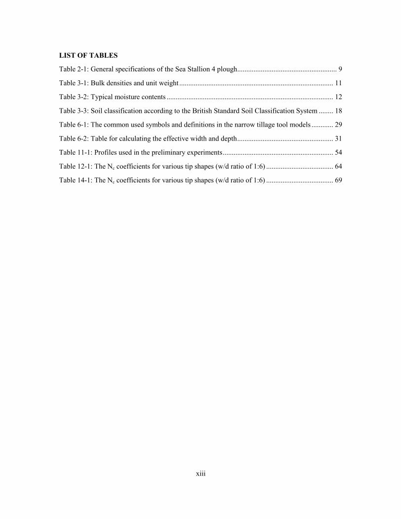
LIST OF TABLES
Table 2-1: General specifications of the Sea Stallion 4 plough....................................................... 9
Table 3-1: Bulk densities and unit weight ..................................................................................... 11
Table 3-2: Typical moisture contents ............................................................................................ 12
Table 3-3: Soil classification according to the British Standard Soil Classification System ........ 18
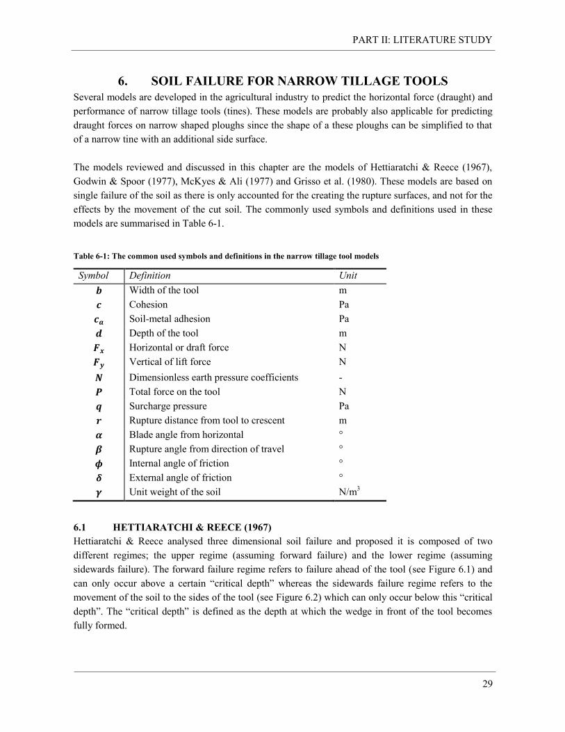
Table 6-1: The common used symbols and definitions in the narrow tillage tool models ............ 29
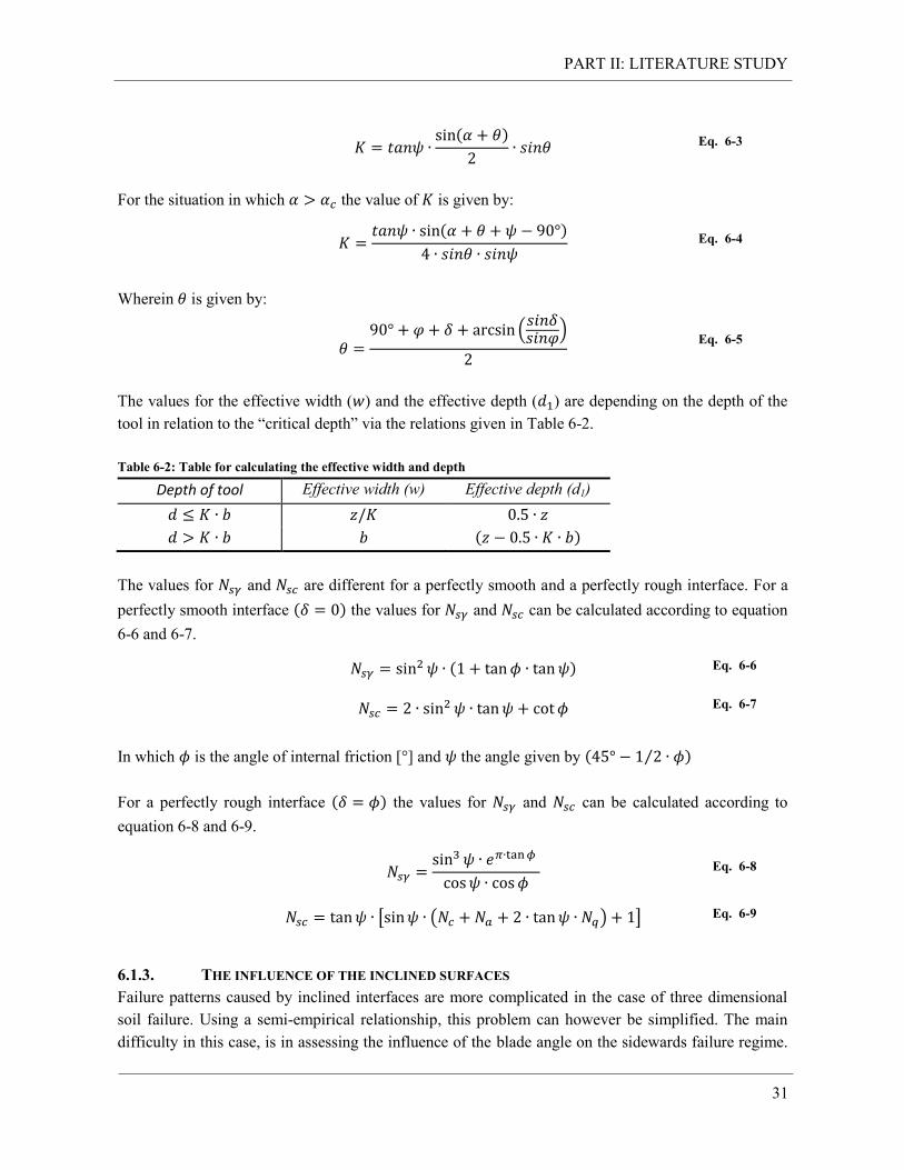
Table 6-2: Table for calculating the effective width and depth ..................................................... 31
Table 11-1: Profiles used in the preliminary experiments ............................................................. 54
Table 12-1: The Nc coefficients for various tip shapes (w/d ratio of 1:6) ..................................... 64
Table 14-1: The Nc coefficients for various tip shapes (w/d ratio of 1:6) ..................................... 69

xiv
xv
LIST OF FIGURES
Figure 1.1: Main analysed ploughing variables............................................................................... 3
Figure 2.1: Burial Protection Index for various soil conditions (Mole et al, 1997)......................... 7
Figure 2.2: Mechanical trencher (VBMS) ....................................................................................... 8
Figure 2.3: Jetting sledge (VBMS) .................................................................................................. 8
Figure 2.4: V-Shaped plough (Ecosse) ............................................................................................ 8
Figure 2.5: Narrow shaped plough (VBMS) ................................................................................... 8
Figure 2.6: The geometry of the Sea Stallion 4 plough (VBMS) .................................................... 9
Figure 3.1: Atterberg limits (Barnes, 2010) .................................................................................. 13
Figure 3.2: Plasticity chart (Barnes, 2010) .................................................................................... 14
Figure 3.3: Stresses on a soil element ........................................................................................... 15
Figure 3.4: Mohr-Coulomb failure ................................................................................................ 16
Figure 3.5: Undrained failure ........................................................................................................ 17
Figure 3.6: Adhesion factors for driven piles (Tomlinson, 1970) ................................................. 18
Figure 4.1: Overview literature study ............................................................................................ 23
Figure 5.1: Strip foundation .......................................................................................................... 24
Figure 5.2: Influence of depth on sliding surfaces ........................................................................ 25
Figure 5.3: Plastic zones in a deep foundation of purely cohesive material (Meyerhof, 1951) .... 26
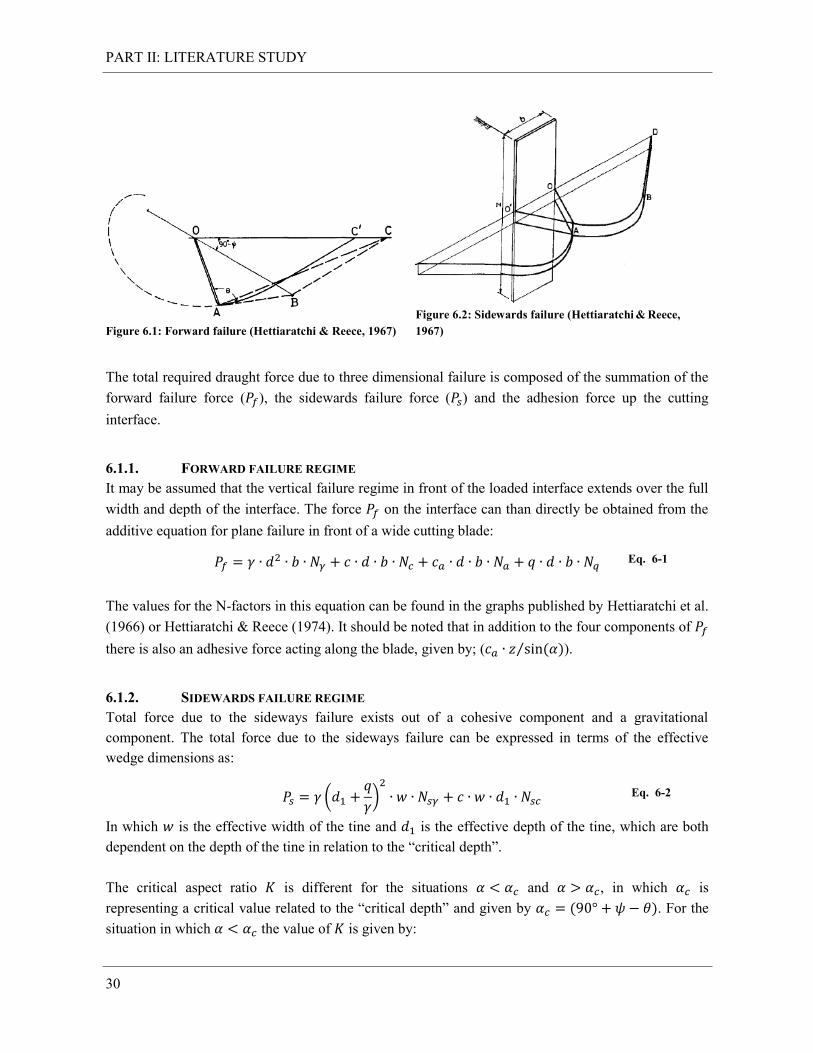
Figure 6.1: Forward failure (Hettiaratchi & Reece, 1967) ............................................................ 30
Figure 6.2: Sidewards failure (Hettiaratchi & Reece, 1967) ......................................................... 30
Figure 6.3: Conceptual mechanism of soil failure (Godwin & Spoor, 1977) ................................ 32
Figure 6.4: Crescent failure geometry (Godwin & Spoor, 1977) .................................................. 33
Figure 6.5: 3D view crescent failure (Godwin & Spoor) .............................................................. 34
Figure 6.6: Side view crescent failure (Godwin & Spoor) ............................................................ 34
Figure 6.7: Dimensionless N factors for lateral failure (Godwin & Spoor, 1977) ........................ 35
Figure 6.8: Proposed soil failure (McKyes & Ali, 1977) .............................................................. 36
Figure 6.9: Forces on the soil segments (McKyes & Ali, 1977) ................................................... 36
Figure 7.1: Soil cutting by straight blades (Reece & Grinsted, 1986) ........................................... 41
xvi
Figure 8.1: The formation of compacted cores in front of various cutting interfaces (Zelenin,
1950) .............................................................................................................................................. 45
Figure 8.2: The four different cutting interfaces used in the experiments a): 45° Triangular (T4),
b): Elliptical (T3), c): Flat (T2) and d) 90° Triangular (T1) (Sharifat, 1999) ................................ 45
Figure 8.3: The used energy by the four different tools at a soil moisture content of 11.2%, a
Cone index of 300 kPa and speeds of 10, 15, 20 and 25 km/hr (Sharifat, 1999) .......................... 46
Figure 8.4: The used energy by the four different tools at a soil moisture content of 15.1%, a
Cone index of 300 kPa and speeds of 10, 15, 20 and 25 km/hr (Sharifat, 1999) .......................... 46
Figure 9.1: The shear planes during failure ................................................................................... 47
Figure 10.1: Parameters used in the base prediction model .......................................................... 50
Figure 11.1: Sketch of the preliminary experimental setup ........................................................... 53
Figure 11.2: Profile shapes analysed in the preliminary experiments ........................................... 54
Figure 11.3: The setup to push the box into the clay ..................................................................... 55
Figure 11.4: The box pushed halfway into the clay blocks ........................................................... 55
Figure 11.5: Pushing the profile through the clay ......................................................................... 55
Figure 11.6: Clay after the starting hole is made ........................................................................... 55
Figure 11.7: Preparations for marking ........................................................................................... 56
Figure 11.8: Clay box after marking ............................................................................................. 56
Figure 11.9: The complete experimental setup ............................................................................. 56
Figure 11.10: The clay box into the experimental setup ............................................................... 56
Figure 11.11: Setup to measure the trenched surface .................................................................... 57
Figure 11.12: The height profile of the trenched surface .............................................................. 57
Figure 11.13: The field vane ......................................................................................................... 57
Figure 11.14: The measuring locations ......................................................................................... 57
Figure 11.15: Lay-out of the test report ......................................................................................... 58
Figure 12.1: Overview of the variables and influences analysed with the results of the preliminary
experiments ................................................................................................................................... 59
Figure 12.2: Deformation profile flat frontal shape ...................................................................... 64
Figure 12.3: Deformation profile circular frontal shape ................................................................ 64
Figure 12.4: Deformation profile sharp frontal shape ................................................................... 64
xvii
Figure 12.5: Deformation profile frontal edge of 45° ................................................................... 64

xviii
xix
LIST OF GRAPHS
Graph 12.1: Repeatability (su = +/- 33 kPa, vavg = +/- 2.5 mm/s) .................................................. 60
Graph 12.2: Length influence (su = +/- 33 kPa, Nc = 10, αa = 0.34, vavg = +/- 2.5 mm/s) ............... 60
Graph 12.3: Size influence (su = +/- 33 kPa, Nc = 10, αa = 0.34, vavg = +/- 2.5 mm/s) ................... 61
Graph 12.4: Tip influence, cylinder compared to blunt (su = +/- 33 kPa, Nc = 10, αa = 0.34, vavg =
+/ 2.5 mm/s) .................................................................................................................................. 62
Graph 12.5: Tip influence, 90° and 45° sharp edged tip compared to blunt ................................. 63
Graph 12.6: Graph showing the influence of the joints between the clay blocks ......................... 65
Graph 13.1: Overview measured and predicted forces (su = +/- 33 kPa, αa = 0.34, vavg = +/- 2.5
mm/s) ............................................................................................................................................. 67
Graph 13.2: Relation between measured and predicted forces (su = +/- 33 kPa, αa = 0.34, vavg = +/-
2.5 mm/s) ....................................................................................................................................... 67

xx
PART I: INTRODUCTION
1
PART I: INTRODUCTION
PART I: INTRODUCTION
2
1. INTRODUCTION
This thesis research has been performed under the authority of VolkerWessels Boskalis Marine
Solutions (VBMS) and Koninklijke Boskalis Westminster N.V. During the development of the exact
research objectives it appeared that both VBMS and Boskalis had an interest in the research topic
making a multi company thesis research possible.
1.1 VOLKERWESSELS BOSKALIS MARINE SOLUTIONS
VolkerWessels Boskalis Marine Solutions established a trusted and experienced position as an
international submarine power cable installation contractor, specialised in the intertidal and offshore
markets.
The company was established in 2007 by Visser & Smit Hanab, under the name of Visser and Smit
Marine Contracting (VSMC). Onward establishment the company served as an independent company
within the VolkerWessels group until the year 2013. In that year VolkerWessels and Royal Boskalis
Westminster N.V. decided to combine their forces in the field of offshore cable installation by the
establishment of a 50/50% joint venture in the company. As a result the name of the company was
changed to VolkerWessels Boskalis Marine Solutions in September 2014.
Typical clients of VBMS are electrical power companies, grid operators and companies in the oil and
gas industry. The company provides a full package for installation of cables. Activities executed by
VBMS are:
Installation and burial of export cables
Installation and burial of inter array cables
Inspection, Repair and Maintenance of cables
Construction of land- & outfalls
Construction of offshore cable crossings
1.2 KONINKLIJKE BOSKALIS WESTMINSTER N.V.
Royal Boskalis Westminster N.V. is a leading global maritime services company operating in the
dredging, inland infra, towage, salvage and offshore sectors.
Traditionally Boskalis was a dredging company but with the acquisitions of Smit International,
Fairmount and Dockwise it became also active in towage, salvage and transport and heavy lifting.
After these acquisitions Boskalis is able to provide total solution packages for the major maritime and
offshore challenges.
Main clients of Boskalis are; companies active in the oil and gas industry, port authorities, global and
local governments, shipping companies, international project developers, insurance companies and
mining companies.
PART I: INTRODUCTION
3
1.3 BACKGROUND FOR THE RESEARCH ASSIGNMENT
VBMS uses multiple vessels and tools to execute subsea power cable installation projects. One of
these tools is the Sea Stallion 4 plough, a narrow shaped plough. This plough is capable of burying
submarine power cables up to 3m below the seabed in order to protect them against human and
environmental impacts such as anchors, fishing gear, current and wave action, etc. The Sea Stallion 4
plough features a unique design and has a robust chassis that can withstand continuous tow forces up
to 120 tons.
There are several manufacturers of narrow shaped ploughs, defined as ploughs with a small width-
over-depth ratio. Most of these manufacturers have their own basic geometric design. This raises
questions on the influence of variables in the design of these ploughs on the required pulling force.
The influence of these variables is related to the local soil conditions, for which there is in this
research a special interest to clay soils. Once the influence of the selected variables in the design of
narrow shaped ploughs is known this knowledge can be used to develop and optimised design of the
Sea Stallion 4 plough for ploughing in clay soils.
1.4 MAIN RESEARCH OBJECTIVE
This thesis project aims to create an empirical plough pulling force model by assessing available
theories and models in combination with performing lab experiments examining the influence of
selected variables, during ploughing in clay.
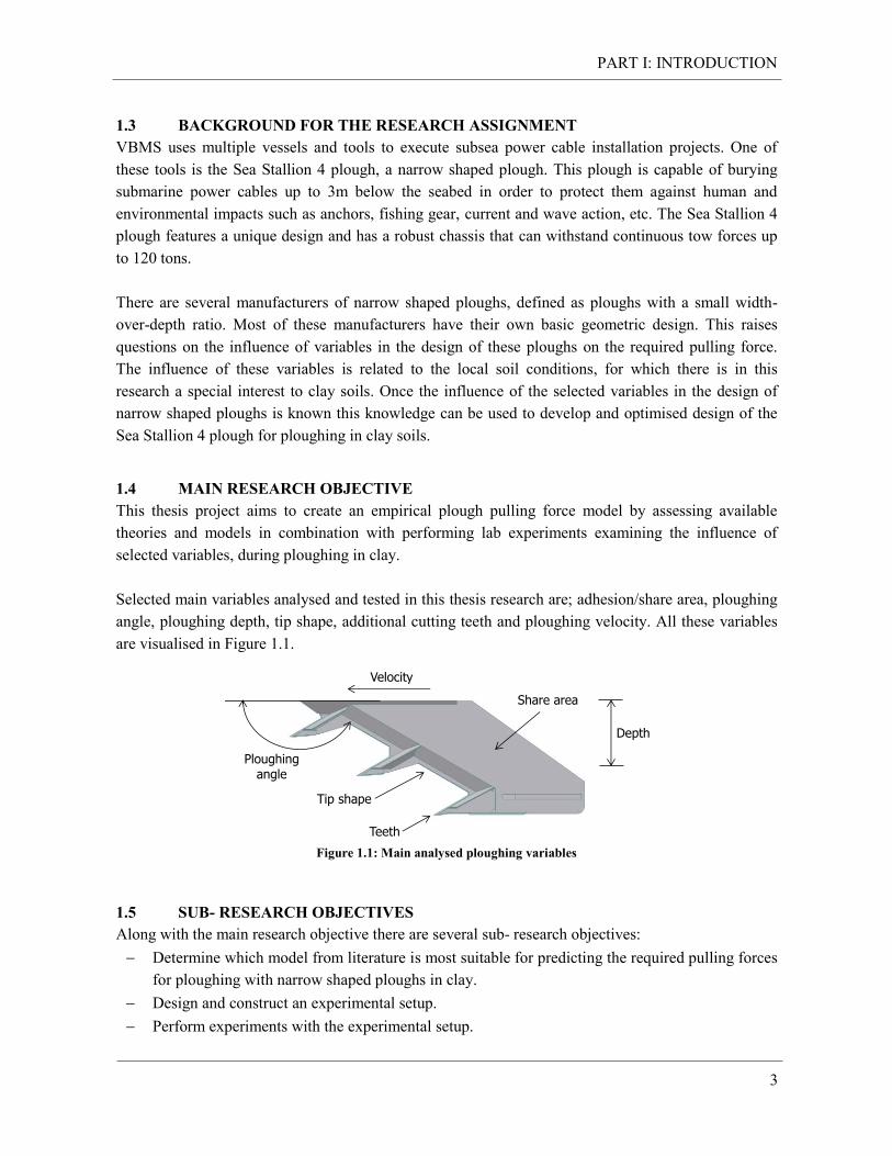
Selected main variables analysed and tested in this thesis research are; adhesion/share area, ploughing
angle, ploughing depth, tip shape, additional cutting teeth and ploughing velocity. All these variables
are visualised in Figure 1.1.
Figure 1.1: Main analysed ploughing variables
1.5 SUB- RESEARCH OBJECTIVES
Along with the main research objective there are several sub- research objectives:
Determine which model from literature is most suitable for predicting the required pulling forces
for ploughing with narrow shaped ploughs in clay.
Design and construct an experimental setup.
Perform experiments with the experimental setup.
Share area
Teeth
Tip shape
Ploughing angle
Velocity
Depth
PART I: INTRODUCTION
4
Create a plough pulling force prediction model.
Develop an optimised design of the Sea Stallion 4 plough, for ploughing in clay.
1.6 RESEARCH PLAN
First, a literature study is performed to study the applicability of already available force prediction
models for narrow shaped ploughs. Concurrently, preliminary experiments are performed in order to
gain insight in magnitudes of the pulling forces occurring during small scale experiments. Once the
literature study is completed and the preliminary experiments are evaluated a main experimental setup
is designed and constructed. In this main experimental setup, the influence of the selected variables is
analysed. The results of these experiments are compared to the results of the models from the literature
study, in order to identify the model most appropriate for predicting the required pulling forces of
narrow shaped ploughs. At last the knowledge gained from the experiments is used to develop an
optimised design of the Sea Stallion 4 plough.
1.7 BOUNDARY CONDITIONS AND LIMITATIONS
The number of experiments to be performed is limited due to the availability of time. This implies not
all parameters influencing the pulling force can be analysed and tested. The variables during
ploughing selected to be analysed and tested in this research are; adhesion/share area, ploughing angle,
ploughing depth, tip shape, additional cutting teeth and ploughing velocity.
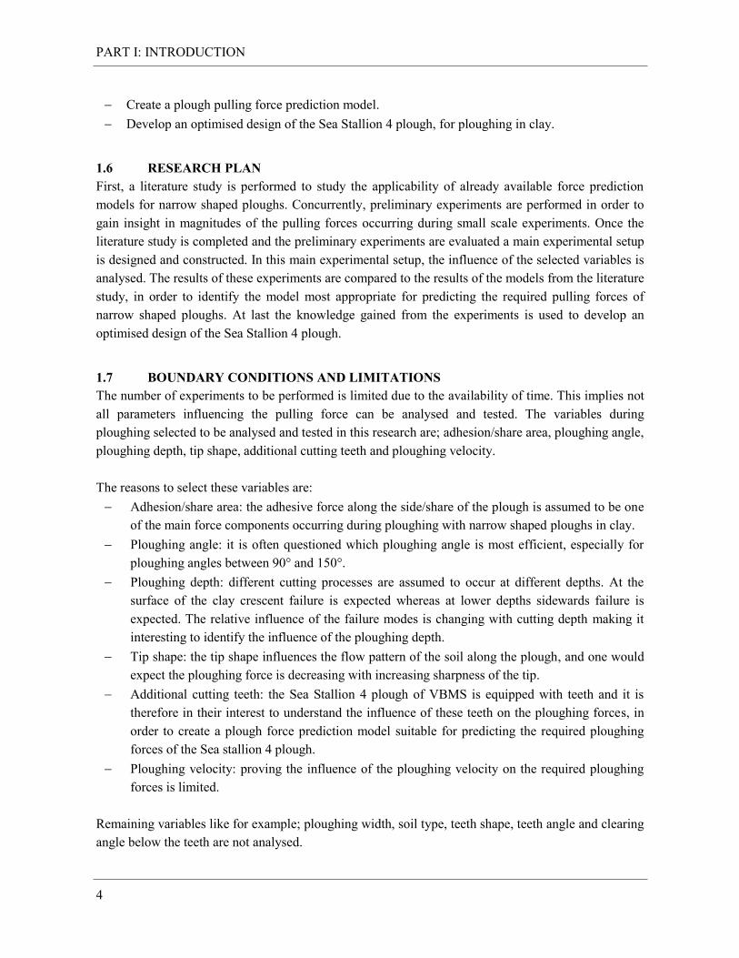
The reasons to select these variables are:
Adhesion/share area: the adhesive force along the side/share of the plough is assumed to be one
of the main force components occurring during ploughing with narrow shaped ploughs in clay.
Ploughing angle: it is often questioned which ploughing angle is most efficient, especially for
ploughing angles between 90° and 150°.
Ploughing depth: different cutting processes are assumed to occur at different depths. At the
surface of the clay crescent failure is expected whereas at lower depths sidewards failure is
expected. The relative influence of the failure modes is changing with cutting depth making it
interesting to identify the influence of the ploughing depth.
Tip shape: the tip shape influences the flow pattern of the soil along the plough, and one would
expect the ploughing force is decreasing with increasing sharpness of the tip.
Additional cutting teeth: the Sea Stallion 4 plough of VBMS is equipped with teeth and it is
therefore in their interest to understand the influence of these teeth on the ploughing forces, in
order to create a plough force prediction model suitable for predicting the required ploughing
forces of the Sea stallion 4 plough.
Ploughing velocity: proving the influence of the ploughing velocity on the required ploughing
forces is limited.
Remaining variables like for example; ploughing width, soil type, teeth shape, teeth angle and clearing
angle below the teeth are not analysed.
PART I: INTRODUCTION
5
Among the different geometries selected to be tested in the experiments sometimes two or more
variables are changed simultaneously as a result of changing only one of the geometrical variables.
This makes it difficult to appoint the exact variable being the origin of a certain difference in the
required pulling force. The different experimental geometries are therefore selected such that the
influences of the selected variables can be distinguished separately as much as possible.
This thesis research should be seen as an encompassing research in which a lot of variables are
reviewed and analysed, and which can be used to appoint the variables and influences to which more
in-depth research should be carried out.
1.8 REPORT STRUCTURE
This repository version of the report is divided in three main parts. The first part is an introductory part
and contains an introduction to cable protection and the material properties of soil. The second part of
the report contains the literature study. In the first chapter of this part an overview of the available
models is given after which the ultimate bearing capacity theory, narrow tine models and subsea
plough models are reviewed in separate chapters. The influences by tip shape and ploughing velocity
are also reviewed in separate chapters. The third part of this report is dedicated to the preliminary
experiments. This part discusses the design of the experimental setup after which the results of the
experiments are analysed. The last parts of the research report are excluded from this repository
version as it contained confidential data and information.
PART I: INTRODUCTION
6
2. INTRODUCTION TO CABLE PROTECTION
This chapter discusses the necessity for subsea cable burial along with commonly used protection
techniques. The burial depth of submarine cables often depends on the requirements stated by clients.
A commonly used method to gain an indication of the required burial depth is the Burial Protection
Index (BPI) which is elaborated in this chapter.
2.1 NECESSITY FOR CABLE PROTECTION
Recent years showed a massive demand for subsea power cables due to the fast development of
offshore renewable energy. Offshore power generators are connected to transformer platforms by
infield cables and these transformer platforms are in turn connected to shore by export cables. All
these cables do need protection to threats since they are too important to be damaged. A list of main
threats to subsea power cables is given below.
Natural threats:
Submarine landslides
Sediment mobility
Seismic activity
Iceberg scour
Human threats:
Fishing activities
Anchoring
Dredging
Dropping objects
2.2 PROTECTION OF SUBSEA CABLES
There are two primary methods used for protection of submarine cables; internal armouring and burial.
A third less commonly used method is protection by rock dumping or placing flexible concrete
mattresses on top of a cable. Costs for this protection method are generally high and therefore only
used for short areas of particular concern, such as crossing and remedial work locations.
Protection by burial is generally considered to be the most practical and reliable method. Cable burial
is often referred to as “trenching” and can be done in different sequences. During ‘pre-trenching’ the
trench is created before a cable is installed whereas during ‘post-trenching’ the trench is created
underneath an already laid cable. During ‘simultaneous laying and burial’ a cable is buried during
lying. A submarine narrow shaped plough typically uses this last burial method.
2.3 BURIAL PROTECTION INDEX
In the eighties cable burial became common practice. A burial depth of 60 cm was often adopted
without assessing level of threat and strength of the soil. Recently, target burial depths have become
more related to possible threats and strength of the soil.
PART I: INTRODUCTION
7
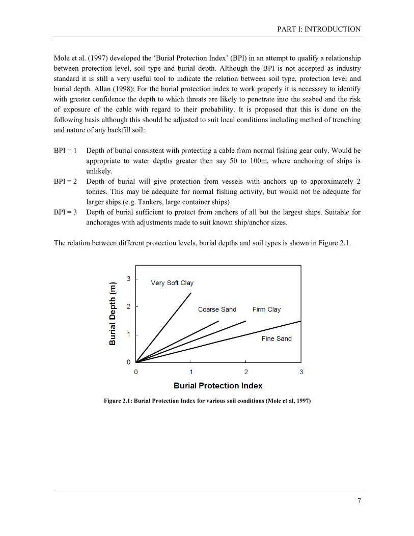
Mole et al. (1997) developed the ‘Burial Protection Index’ (BPI) in an attempt to qualify a relationship
between protection level, soil type and burial depth. Although the BPI is not accepted as industry
standard it is still a very useful tool to indicate the relation between soil type, protection level and
burial depth. Allan (1998); For the burial protection index to work properly it is necessary to identify
with greater confidence the depth to which threats are likely to penetrate into the seabed and the risk
of exposure of the cable with regard to their probability. It is proposed that this is done on the
following basis although this should be adjusted to suit local conditions including method of trenching
and nature of any backfill soil:
BPI = 1 Depth of burial consistent with protecting a cable from normal fishing gear only. Would be
appropriate to water depths greater then say 50 to 100m, where anchoring of ships is
unlikely.
BPI = 2 Depth of burial will give protection from vessels with anchors up to approximately 2
tonnes. This may be adequate for normal fishing activity, but would not be adequate for
larger ships (e.g. Tankers, large container ships)
BPI = 3 Depth of burial sufficient to protect from anchors of all but the largest ships. Suitable for
anchorages with adjustments made to suit known ship/anchor sizes.
The relation between different protection levels, burial depths and soil types is shown in Figure 2.1.
Figure 2.1: Burial Protection Index for various soil conditions (Mole et al, 1997)
PART I: INTRODUCTION
8
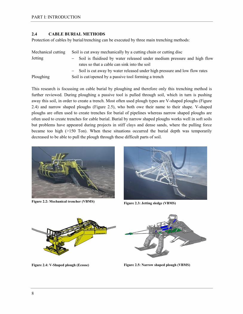
2.4 CABLE BURIAL METHODS
Protection of cables by burial/trenching can be executed by three main trenching methods:
Mechanical cutting Soil is cut away mechanically by a cutting chain or cutting disc
Jetting Soil is fluidised by water released under medium pressure and high flow
rates so that a cable can sink into the soil
Soil is cut away by water released under high pressure and low flow rates
Ploughing Soil is cut/opened by a passive tool forming a trench
This research is focussing on cable burial by ploughing and therefore only this trenching method is
further reviewed. During ploughing a passive tool is pulled through soil, which in turn is pushing
away this soil, in order to create a trench. Most often used plough types are V-shaped ploughs (Figure
2.4) and narrow shaped ploughs (Figure 2.5), who both owe their name to their shape. V-shaped
ploughs are often used to create trenches for burial of pipelines whereas narrow shaped ploughs are
often used to create trenches for cable burial. Burial by narrow shaped ploughs works well in soft soils
but problems have appeared during projects in stiff clays and dense sands, where the pulling force
became too high (>150 Ton). When these situations occurred the burial depth was temporarily
decreased to be able to pull the plough through these difficult parts of soil.
Figure 2.2: Mechanical trencher (VBMS)
Figure 2.3: Jetting sledge (VBMS)
Figure 2.4: V-Shaped plough (Ecosse)
Figure 2.5: Narrow shaped plough (VBMS)
PART I: INTRODUCTION
9
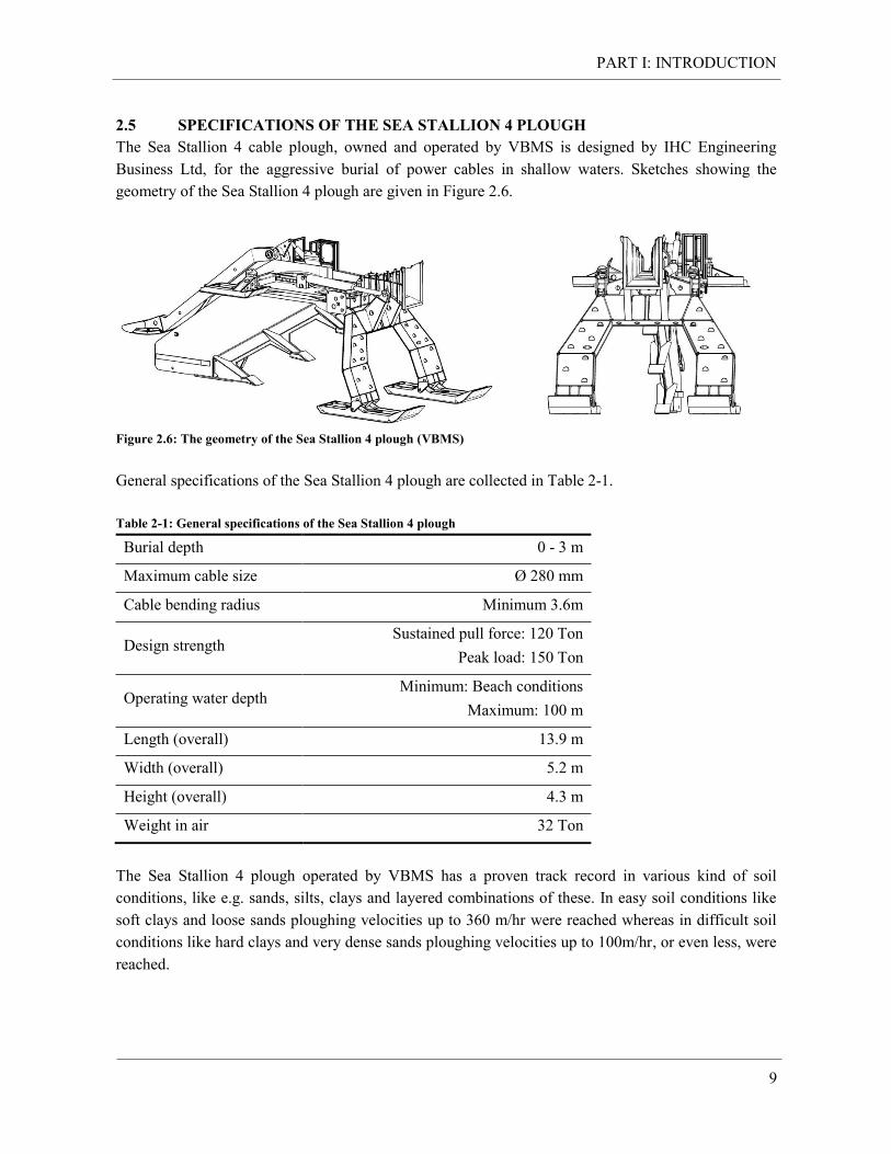
2.5 SPECIFICATIONS OF THE SEA STALLION 4 PLOUGH
The Sea Stallion 4 cable plough, owned and operated by VBMS is designed by IHC Engineering
Business Ltd, for the aggressive burial of power cables in shallow waters. Sketches showing the
geometry of the Sea Stallion 4 plough are given in Figure 2.6.
Figure 2.6: The geometry of the Sea Stallion 4 plough (VBMS)
General specifications of the Sea Stallion 4 plough are collected in Table 2-1.
Table 2-1: General specifications of the Sea Stallion 4 plough
Burial depth 0 - 3 m
Maximum cable size Ø 280 mm
Cable bending radius Minimum 3.6m
Design strength Sustained pull force: 120 Ton
Peak load: 150 Ton
Operating water depth Minimum: Beach conditions
Maximum: 100 m
Length (overall) 13.9 m
Width (overall) 5.2 m
Height (overall) 4.3 m
Weight in air 32 Ton
The Sea Stallion 4 plough operated by VBMS has a proven track record in various kind of soil
conditions, like e.g. sands, silts, clays and layered combinations of these. In easy soil conditions like
soft clays and loose sands ploughing velocities up to 360 m/hr were reached whereas in difficult soil
conditions like hard clays and very dense sands ploughing velocities up to 100m/hr, or even less, were
reached.
PART I: INTRODUCTION
10
3. MATERIAL PROPERTIES OF SOIL
In this chapter the most common parameters to describe the properties and behaviour of clay soils are
described and explained.
3.1 POROSITY (SOIL)
Soils usually consist of particles, water and air. In soil mechanics the space between particles is known
as pores. There are several ways to express the amount of pore space. The most common parameter
describing this amount is porosity, which is defined as:
Eq. 3-1
Porosity [-]
Volume of pores [m3]
Volume of the soil [m3]
For most soils the porosity (n) is in between 0.30 and 0.45. A smaller porosity corresponds with a
denser soil.
3.2 VOID RATIO (SOIL)
A second way in which the amount of pore space can be expressed is void ratio. It is the ratio between
the volume of pores and the volume of particles.
Eq. 3-2
Void ratio [-]
Volume of pores [m3]
Volume of solids [m3]
3.3 DENSITY (SOIL)
Density of a substance is given by the mass per unit volume of that substance.
Eq. 3-3
Density of the soil [kg/ m3]
Mass of the soil [kg]
Volume of the soil [m3]
PART I: INTRODUCTION
11
The in-situ density of a fully saturated soil can be calculated according:
( ) ( ( )) Eq. 3-4
Density in-situ [kg/m3]
Density of water [kg/m3]
Density of solids [kg/m3]
An overview of typical bulk density values for different types of soils is given in Table 3-1.
3.4 UNIT WEIGHT (SOIL)
Unit weight is defined as the weight per unit volume:
Eq. 3-5
Unit weight [N/m3]
Weight of the soil [N]
Gravitational constant [m/s2]
An overview of typical unit weight values for different types of soils is given in Table 3-1.
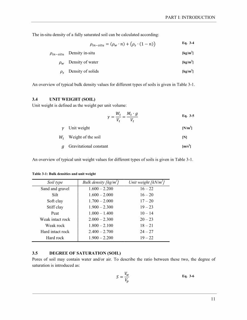
Table 3-1: Bulk densities and unit weight
Soil type Bulk density [kg/m3] Unit weight [kN/m
3]
Sand and gravel 1.600 – 2.200 16 – 22
Silt 1.600 – 2.000 16 – 20
Soft clay 1.700 – 2.000 17 – 20
Stiff clay 1.900 – 2.300 19 – 23
Peat 1.000 – 1.400 10 – 14
Weak intact rock 2.000 – 2.300 20 – 23
Weak rock 1.800 – 2.100 18 – 21
Hard intact rock 2.400 – 2.700 24 – 27
Hard rock 1.900 – 2.200 19 – 22
3.5 DEGREE OF SATURATION (SOIL)
Pores of soil may contain water and/or air. To describe the ratio between these two, the degree of
saturation is introduced as:
Eq. 3-6

PART I: INTRODUCTION
12
Degrees of saturation [-]
Volume of water [m3]
Volume of pores [m3]
In offshore and near beach conditions of ploughing operations, clay is often assumed to be fully
saturated. This is important to note since it ensures there is no air present inside the clay.
3.6 MOISTURE CONTENT (SOIL)
The moisture content, or water content, is the ratio between the mass of water to the mass of solid
particles and is a valuable indicator for the state of a soil and its behaviour.
Eq. 3-7
Moisture content [%]
Mass of water [kg]
Mass of solids [kg]
Some typical values of moisture content are given in Table 3-2.
Table 3-2: Typical moisture contents
Soil Types Moisture content [%]
Moist sand 5 – 15
‘Wet’ sand 15 – 25
Moist silt 10 – 20
‘Wet’ silt 20 – 30
Normally consolidated clay – low plasticity 20 – 40
Normally consolidated clay – high plasticity 50 – 90
Overconsolidated clay – low plasticity 10 – 20
Overconsolidated clay – high plasticity 20 – 40
Organic clay 50 – 200
Extremely high plasticity clay 100 – 200
Peats 100 - > 1000
3.7 ATTERBERG LIMITS (CLAY)
Atterberg limits are used to describe the nature of a fine-grained soil. Depending on the moisture
content of the soil, it may appear in four states: solid, semi-solid, plastic and liquid. In each of these
four states the behaviour of the soil is different and so are its properties.
PART I: INTRODUCTION
13
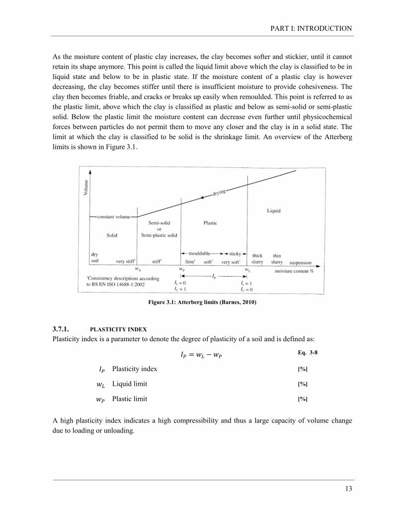
As the moisture content of plastic clay increases, the clay becomes softer and stickier, until it cannot
retain its shape anymore. This point is called the liquid limit above which the clay is classified to be in
liquid state and below to be in plastic state. If the moisture content of a plastic clay is however
decreasing, the clay becomes stiffer until there is insufficient moisture to provide cohesiveness. The
clay then becomes friable, and cracks or breaks up easily when remoulded. This point is referred to as
the plastic limit, above which the clay is classified as plastic and below as semi-solid or semi-plastic
solid. Below the plastic limit the moisture content can decrease even further until physicochemical
forces between particles do not permit them to move any closer and the clay is in a solid state. The
limit at which the clay is classified to be solid is the shrinkage limit. An overview of the Atterberg
limits is shown in Figure 3.1.
Figure 3.1: Atterberg limits (Barnes, 2010)
3.7.1. PLASTICITY INDEX
Plasticity index is a parameter to denote the degree of plasticity of a soil and is defined as:
Eq. 3-8
Plasticity index [%]
Liquid limit [%]
Plastic limit [%]
A high plasticity index indicates a high compressibility and thus a large capacity of volume change
due to loading or unloading.
PART I: INTRODUCTION
14
3.7.2. LIQUIDITY INDEX
Liquidity index is an indicator for the position of the moisture content in relation to the Atterberg
limits. The liquidity index is defined as:
Eq. 3-9
Liquidity index [%]
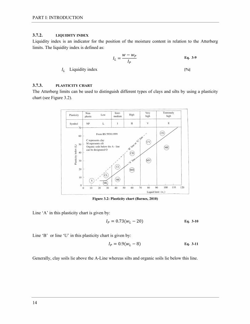
3.7.3. PLASTICITY CHART
The Atterberg limits can be used to distinguish different types of clays and silts by using a plasticity
chart (see Figure 3.2).
Figure 3.2: Plasticity chart (Barnes, 2010)
Line ‘A’ in this plasticity chart is given by:
( ) Eq. 3-10
Line ‘B’ or line ‘U’ in this plasticity chart is given by:
( ) Eq. 3-11
Generally, clay soils lie above the A-Line whereas silts and organic soils lie below this line.
PART I: INTRODUCTION
15
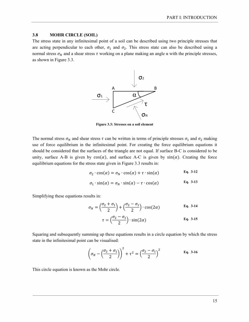
3.8 MOHR CIRCLE (SOIL)
The stress state in any infinitesimal point of a soil can be described using two principle stresses that
are acting perpendicular to each other, and . This stress state can also be described using a
normal stress and a shear stress working on a plane making an angle α with the principle stresses,
as shown in Figure 3.3.
Figure 3.3: Stresses on a soil element
The normal stress and shear stress can be written in terms of principle stresses and making
use of force equilibrium in the infinitesimal point. For creating the force equilibrium equations it
should be considered that the surfaces of the triangle are not equal. If surface B-C is considered to be
unity, surface A-B is given by ( ), and surface A-C is given by ( ). Creating the force
equilibrium equations for the stress state given in Figure 3.3 results in:
( ) ( ) ( ) Eq. 3-12
( ) ( ) ( ) Eq. 3-13
Simplifying these equations results in:
(
) (
) ( ) Eq. 3-14
(
) ( ) Eq. 3-15
Squaring and subsequently summing up these equations results in a circle equation by which the stress
state in the infinitesimal point can be visualised:
( (
))
(
)
Eq. 3-16
This circle equation is known as the Mohr circle.
α
σ2
σ1
τ
σN
A B
C

PART I: INTRODUCTION
16
3.9 MOHR-COULOMB FAILURE CRITERION (SOIL)
The Mohr-Coulomb failure criterion represents a linear envelope that is obtained from circular plots of
the shear strength versus the applied normal stress. Once several failure conditions under different
stress states are known, they can be visualised using their Mohr circles in order to determine the
failure line of the Mohr-Coulomb failure criterion, as is shown in Figure 3.4.
cφ
τ
σ σ1 σ1 σ2 σ2
Failure line
Figure 3.4: Mohr-Coulomb failure
The failure line of the Mohr-Coulomb failure criterion is represented by:
( ) Eq. 3-17
Shear strength at failure [Pa]
Normal stress [Pa]
Cohesion [Pa]
Internal friction angle [°]
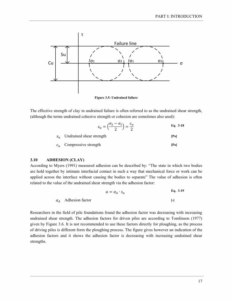
3.9.1. UNDRAINED SOIL FAILURE (SOIL)
During undrained failure a load is applied so quickly to the clay, that there is no expelling of water out
of the pores of the clay. This means that the applied load is taken by the water in the pores instead of
by the grains of the clay. As a result the effective strength of the clay is independent of the applied
load. The Mohr circles of various undrained failure conditions can be drawn in one figure (see Figure
3.5). In this figure the resulting failure line is nearly horizontal from which can be concluded the angle
of internal friction is close to zero. Consequently it is often referred to as the failure principle,
or a material that is behaving frictionless. According to the Mohr-Coulomb failure criterion it can be
concluded the maximum allowable shear strength (undrained shear strength) is independent of the
applied load and equal to half the compressive strength of the material.
PART I: INTRODUCTION
17
Figure 3.5: Undrained failure
The effective strength of clay in undrained failure is often referred to as the undrained shear strength,
(although the terms undrained cohesive strength or cohesion are sometimes also used):
(
)
Eq. 3-18
Undrained shear strength [Pa]
Compressive strength [Pa]
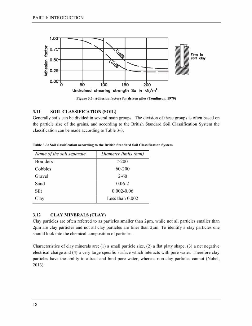
3.10 ADHESION (CLAY)
According to Myers (1991) measured adhesion can be described by: “The state in which two bodies
are hold together by intimate interfacial contact in such a way that mechanical force or work can be
applied across the interface without causing the bodies to separate” The value of adhesion is often
related to the value of the undrained shear strength via the adhesion factor:
Eq. 3-19
Adhesion factor [-]
Researchers in the field of pile foundations found the adhesion factor was decreasing with increasing
undrained shear strength. The adhesion factors for driven piles are according to Tomlinson (1977)
given by Figure 3.6. It is not recommended to use these factors directly for ploughing, as the process
of driving piles is different form the ploughing process. The figure gives however an indication of the
adhesion factors and it shows the adhesion factor is decreasing with increasing undrained shear
strengths.
Su
τ
σ σ1 σ1σ2 σ2
Failure line
Cu
PART I: INTRODUCTION
18
Figure 3.6: Adhesion factors for driven piles (Tomlinson, 1970)
3.11 SOIL CLASSIFICATION (SOIL)
Generally soils can be divided in several main groups.. The division of these groups is often based on
the particle size of the grains, and according to the British Standard Soil Classification System the
classification can be made according to Table 3-3.
Table 3-3: Soil classification according to the British Standard Soil Classification System
Name of the soil separate Diameter limits (mm)
Boulders >200
Cobbles 60-200
Gravel 2-60
Sand 0.06-2
Silt 0.002-0.06
Clay Less than 0.002
3.12 CLAY MINERALS (CLAY)
Clay particles are often referred to as particles smaller than 2μm, while not all particles smaller than
2μm are clay particles and not all clay particles are finer than 2μm. To identify a clay particles one
should look into the chemical composition of particles.
Characteristics of clay minerals are; (1) a small particle size, (2) a flat platy shape, (3) a net negative
electrical charge and (4) a very large specific surface which interacts with pore water. Therefore clay
particles have the ability to attract and bind pore water, whereas non-clay particles cannot (Nobel,
2013).
PART I: INTRODUCTION
19
3.13 SOIL STRUCTURE OF CLAY (CLAY)
Clay mineral particles are very small and only visible with a microscope. Soils, in which clay particles
predominate, have cohesion, plasticity and a low permeability. Clay soils have very complex
microstructures which are affected by the type of clay minerals and their amounts, the proportion of
silt and sand, the deposition environment and the chemical nature of the pore water.
The macrostructure of clay soils can be seen by eye and generally consist of features that are
originating from deposition like inclusions, partings, laminations and varves and features produced
after deposition like fissures, joints, cracks, and root holes.
To understand the behaviour of a clay (shear strength, compressibility, consolidation, permeability,
shrinkage, etc) one should look into the nature of the microstructure of the soil. The openness of this
microstructure is given by the moisture content, which is a parameter represent the structural nature of
the clay when fully saturated. The liquidity index is used to represent the structural state of the clay, as
it compares the moisture content of the clay to the plastic and liquid limits.
PART I: INTRODUCTION
20
PART II: LITERATURE STUDY
21
PART II: LITERATURE STUDY
PART II: LITERATURE STUDY
22
4. INTRODUCTION LITERATURE STUDY
The main variables during ploughing reviewed in the literature study are;
Adhesion/share area
Ploughing depth
Ploughing angle
Additional cutting teeth
Tip shape
Ploughing velocity
Analytical theories available and applicable for prediction of required cutting forces during ploughing,
or the influence of one of the given variables, are discussed in separate chapters. The theories and
models being reviewed are: the ultimate bearing capacity theory, the narrow tine models, the subsea
plough models, the tip shape influence, and the strain-rate dependent behaviour of clay.
The first theory reviewed is the ultimate bearing capacity theory originating from engineering of
foundations. The strip or foundation area used in this theory can be rotated to vertical to represent the
frontal area of the narrow shaped plough and to calculate the required cutting force by the plough.
Additionally an adhesive force accounting for the adhesion along the side/share area of the plough can
be added to this cutting force in order to predict the required ploughing forces.
The second group of models being reviewed are the narrow tine models, which are originating from
the agricultural industry. The geometries of the narrow shaped ploughs are more or less similar to
these of the narrow tines, making it interesting to analyse the usability of these models.
The last group of models being reviewed are the subsea plough models which are developed in the
eighties of the last century. These models are highly empirical and do have empirical coefficients for
each plough shape in combination with certain soil conditions. Due to this high empirical content they
are not preferred to be used in the plough pulling force model of the narrow shaped ploughs.
Last decades showed an increase in the use of numerical tools for the modelling of soil tillage
processes. Commonly used numerical methods are Finite Element Methods (FEM) and Discrete
Element Methods (DEM). The usability of these methods can be reviewed making numerical models
for the plough geometries to be analysed in the main experimental setup. It would however require too
much time to familiarise with the software using these methods and to develop the numerical models
of the various plough geometries to be analysed in the main experiments.
Only analytical models are reviewed in the literature study, in order to keep the plough pulling force
model as simple as possible. The analytical models predicting the required ploughing force, the
influence by the tip shape, and the influence by ploughing velocity are reviewed separately. No
models are available predicting the influence of certain tip shapes on the required pulling force, but
research by Sharifat (1999) showed the required pulling force by sharp tip shapes was lower compared
to blunt tip shapes. The influence of the ploughing velocity on the required ploughing force is
PART II: LITERATURE STUDY
23
originating from the strain-rate dependent behaviour of clay. Various researchers developed models
accounting for this behaviour on the undrained shear strength of the clay, using exponential or
logarithmic functions.
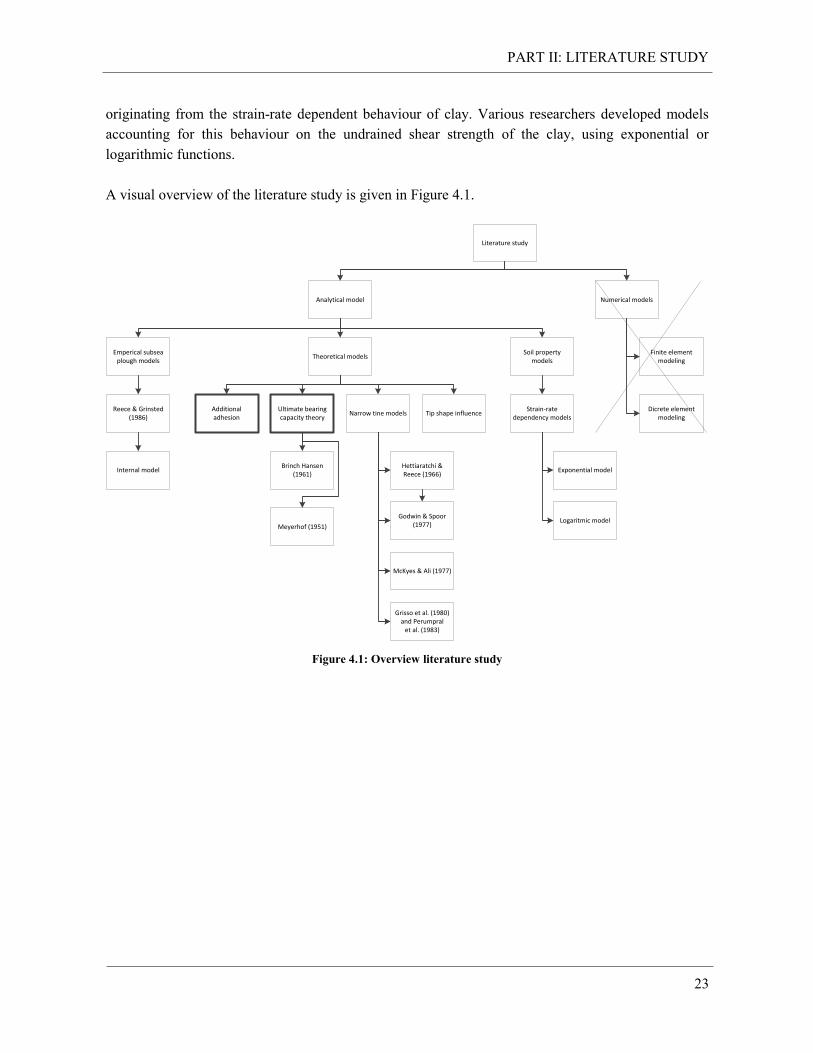
A visual overview of the literature study is given in Figure 4.1.
Figure 4.1: Overview literature study
Analytical model
Emperical subsea plough models
Theoretical models
Reece & Grinsted (1986)
Internal model
Additional adhesion
Ultimate bearing capacity theory
Narrow tine models
Soil property models
Tip shape influenceStrain-rate
dependency models
Logaritmic model
Exponential modelBrinch Hansen
(1961)Hettiaratchi & Reece (1966)
Godwin & Spoor (1977)
McKyes & Ali (1977)
Grisso et al. (1980) and Perumpral
et al. (1983)
Meyerhof (1951)
Literature study
Numerical models
Finite element modeling
Dicrete element modeling
PART II: LITERATURE STUDY
24
5. ULTIMATE BEARING CAPACITY THEORY
This chapter describes the ultimate bearing capacity theory used for foundation designs. The strip or
foundation area used in this theory can be rotated to vertical to represent the frontal area of the narrow
shaped plough and to calculate the required cutting force by the plough.
5.1 ULTIMATE BEARING CAPACITY
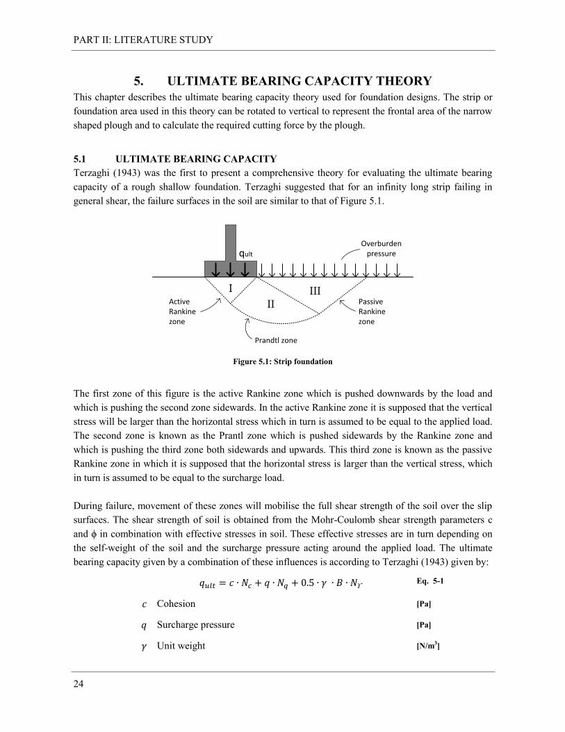
Terzaghi (1943) was the first to present a comprehensive theory for evaluating the ultimate bearing
capacity of a rough shallow foundation. Terzaghi suggested that for an infinity long strip failing in
general shear, the failure surfaces in the soil are similar to that of Figure 5.1.
I
IIIII
Active Rankine zone
Prandtl zone
Passive Rankine zone
Overburden pressureqult
Figure 5.1: Strip foundation
The first zone of this figure is the active Rankine zone which is pushed downwards by the load and
which is pushing the second zone sidewards. In the active Rankine zone it is supposed that the vertical
stress will be larger than the horizontal stress which in turn is assumed to be equal to the applied load.
The second zone is known as the Prantl zone which is pushed sidewards by the Rankine zone and
which is pushing the third zone both sidewards and upwards. This third zone is known as the passive
Rankine zone in which it is supposed that the horizontal stress is larger than the vertical stress, which
in turn is assumed to be equal to the surcharge load.
During failure, movement of these zones will mobilise the full shear strength of the soil over the slip
surfaces. The shear strength of soil is obtained from the Mohr-Coulomb shear strength parameters c
and ϕ in combination with effective stresses in soil. These effective stresses are in turn depending on
the self-weight of the soil and the surcharge pressure acting around the applied load. The ultimate
bearing capacity given by a combination of these influences is according to Terzaghi (1943) given by:
Eq. 5-1
Cohesion [Pa]
Surcharge pressure [Pa]
Unit weight [N/m3]
PART II: LITERATURE STUDY
25
Width of the foundation [m]
The bearing capacity factors , and are depending on the internal friction angle and can be
found in Appendix A.
5.1.1. SHAPE FACTORS
Equation 5-1 is only valid for infinite long strips where shearing is assumed to take place in a two-
dimensional plane. For rectangular foundations shearing will however also occur at the short ends of
the rectangle, producing “end effects”. In order to account for this “end effects” shape factors are
added to equation 5-1:
Eq. 5-2
The shape factors for rectangles with a width B and a length L are according to Brinch Hansen (1970)
given by:
Eq. 5-3
Eq. 5-4
Eq. 5-5
To calculate these shape factors the shortest sides should be assumed as width.
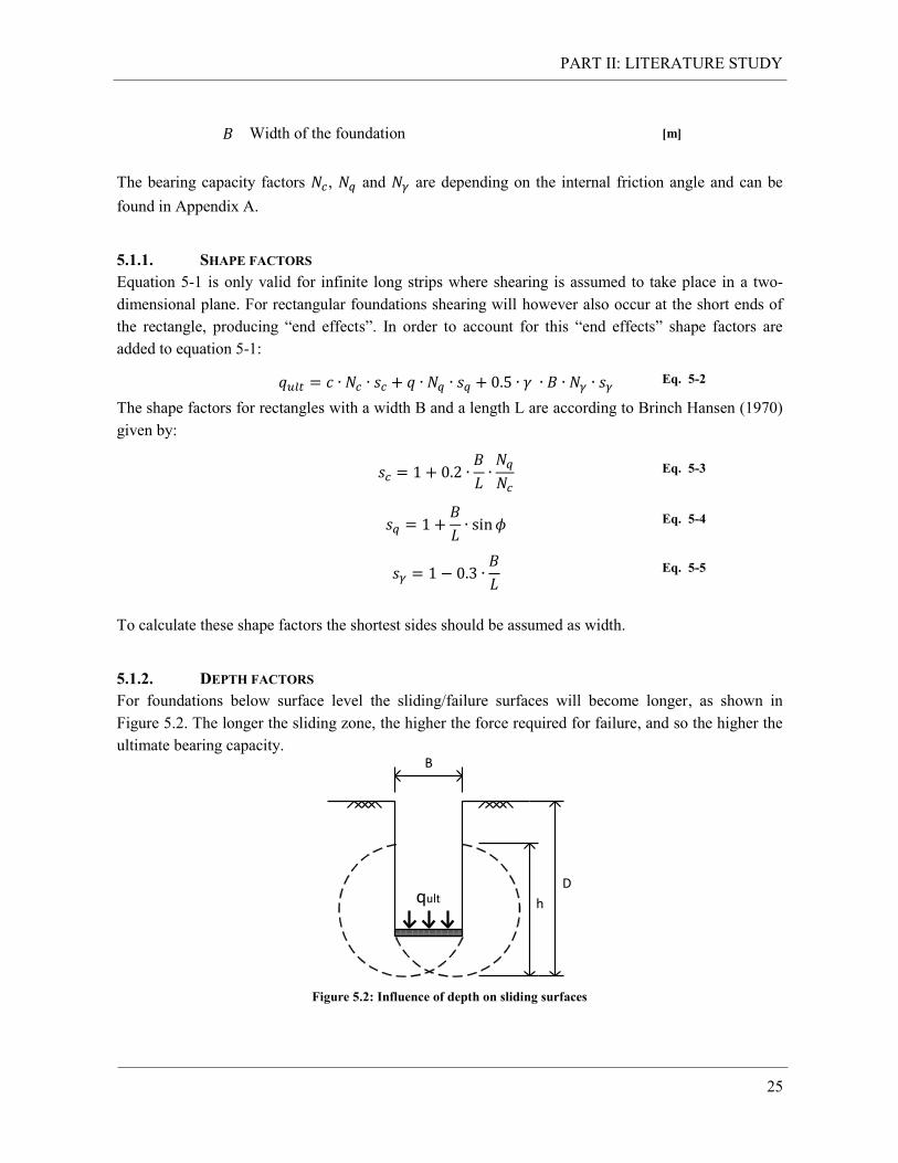
5.1.2. DEPTH FACTORS
For foundations below surface level the sliding/failure surfaces will become longer, as shown in
Figure 5.2. The longer the sliding zone, the higher the force required for failure, and so the higher the
ultimate bearing capacity.
Figure 5.2: Influence of depth on sliding surfaces
qult
B
h
D
PART II: LITERATURE STUDY
26
To account for the influence of the depth on the ultimate bearing capacity, a depth factor is added to
equation 5-2, as is shown in the equation 5-6.
Eq. 5-6
The depth factors proposed by Brinch Hansen (1970) are given by:
(
) Eq. 5-7
( ) (
) Eq. 5-8
Eq. 5-9
5.2 MEYERHOF (1951)
The ultimate bearing capacity theory by Terzaghi (1943) is adopted by Meyerhof (1951) in order to
create an equation describing the ultimate bearing capacity of an infinite long strip at a certain
foundation depth, D, in a purely cohesive material:
Eq. 5-10
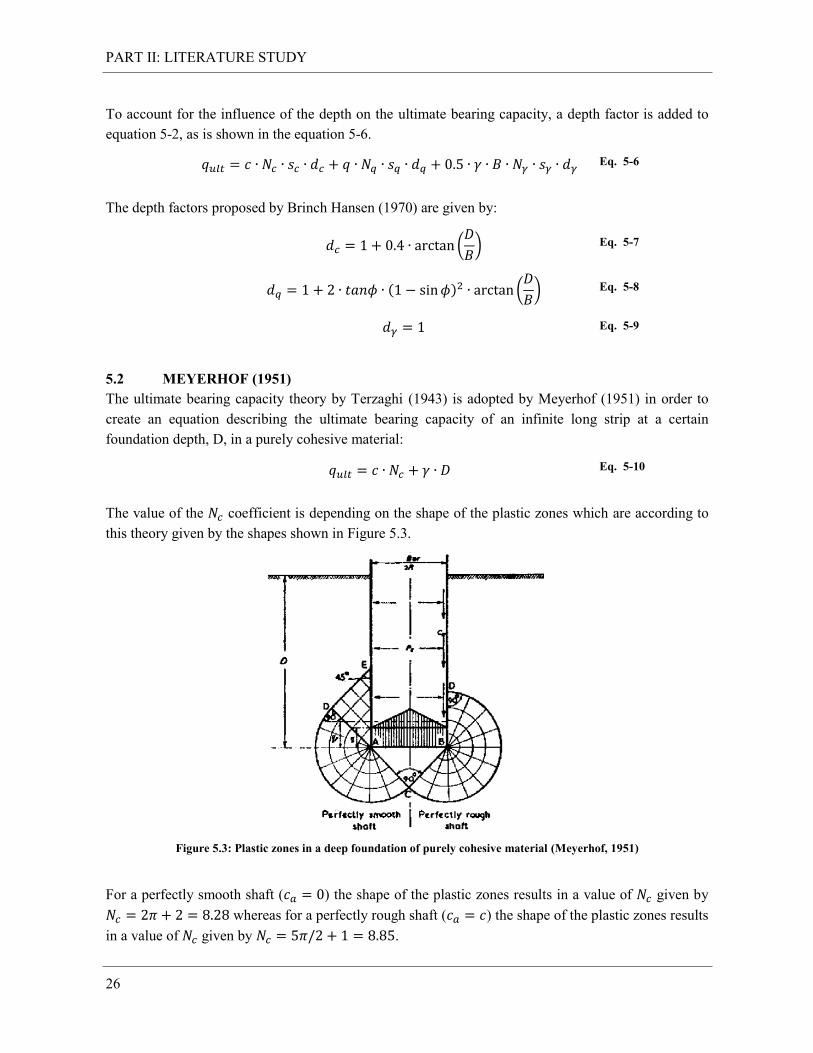
The value of the coefficient is depending on the shape of the plastic zones which are according to
this theory given by the shapes shown in Figure 5.3.
Figure 5.3: Plastic zones in a deep foundation of purely cohesive material (Meyerhof, 1951)
For a perfectly smooth shaft ( ) the shape of the plastic zones results in a value of given by
whereas for a perfectly rough shaft ( ) the shape of the plastic zones results
in a value of given by .
PART II: LITERATURE STUDY
27
5.3 CUTTING FORCE DURING PLOUGHING
To use the ultimate bearing capacity theory for predicting the cutting forces during ploughing, the strip
used in the bearing capacity theory can be rotated to vertical to represent the frontal area of the plough.
By rotating the strip the surcharge pressure can be replaced by the horizontal soil pressure, which
influence is assumed to be zero. In addition, the weight of the soil will act perpendicular to the sliding
surfaces, making its influence negligible.
The frontal area of the plough will not be represented by an infinite long strip but by a long and
narrow rectangle. The upper side of the plough is connected to the plough frame above the soil and so
no “end effect” is expected on this side of the rectangle whereas at the bottom side one “end effect” is
expected. The shape factor of equation 5-3 is accounting for two “end effects” and is rewritten to
equation 5-11 in order to account for only one “end effect”.
Eq. 5-11
The influence by the foundation is also rotated to vertical. As the plough is completely enclosed by
clay during the ploughing process, the upper limit, , of the depth factor should be used in the
equation to calculate the ultimate pressure in front of the plough.
( )⁄
[ (
)] Eq. 5-12
Taking both effects into account, the ultimate bearing capacity pressure that is generated in front of the
plough can be calculated by:
Eq. 5-13
The ultimate bearing pressure that can be generated in front of the plough can also be calculated using
the ultimate bearing capacity theory as proposed by Meyerhof (1951). As the strip in this theory is
rotated to vertical the influence by the weight of the soil is zero. The ultimate bearing pressure that can
be generated in front of the plough is given by:
Eq. 5-14
Wherein is given by 8.85.
Using one of both ultimate bearing capacity models, the cutting force in front of the plough can be
calculated by:
Eq. 5-15

PART II: LITERATURE STUDY
28
5.4 APPLICABILITY OF THE MODEL
Foundations are not supposed to move whereas the narrow shaped ploughs are designed to move. This
means that the velocity effects are neglected in the ultimate bearing capacity theory. As the strength of
clay is known to increase with increasing deformation rates, the forces calculated by the ultimate
bearing capacity theory are the minimum expected cutting forces during ploughing.
The ultimate bearing capacity pressure that can be generated in front of the narrow shaped plough is
based on the simplification of the plough to a very narrow rectangle with a flat tip. The plough has
however a more streamlined tip that will probably reduce the required pulling force. The influence of
the tip shapes is not accounted for in the ultimate bearing capacity model, probably resulting in
conservative predictions for the cutting forces.
The narrow shaped plough is pushing the top of the cut soil upwards instead of sidewards, since this
requires a lower force. This effect is not accounted for in the ultimate bearing capacity model which
probably results in conservative predictions for the cutting forces.
With the discussed influences borne in mind it can be concluded the cutting force of the narrow
shaped ploughs is probably smaller than the values as calculated with the ultimate bearing capacity
theory.
PART II: LITERATURE STUDY
29
6. SOIL FAILURE FOR NARROW TILLAGE TOOLS
Several models are developed in the agricultural industry to predict the horizontal force (draught) and
performance of narrow tillage tools (tines). These models are probably also applicable for predicting
draught forces on narrow shaped ploughs since the shape of a these ploughs can be simplified to that
of a narrow tine with an additional side surface.
The models reviewed and discussed in this chapter are the models of Hettiaratchi & Reece (1967),
Godwin & Spoor (1977), McKyes & Ali (1977) and Grisso et al. (1980). These models are based on
single failure of the soil as there is only accounted for the creating the rupture surfaces, and not for the
effects by the movement of the cut soil. The commonly used symbols and definitions used in these
models are summarised in Table 6-1.
Table 6-1: The common used symbols and definitions in the narrow tillage tool models
Symbol Definition Unit
Width of the tool m
Cohesion Pa
Soil-metal adhesion Pa
Depth of the tool m
Horizontal or draft force N
Vertical of lift force N
Dimensionless earth pressure coefficients -
Total force on the tool N
Surcharge pressure Pa
Rupture distance from tool to crescent m
Blade angle from horizontal °
Rupture angle from direction of travel °
Internal angle of friction °
External angle of friction °
Unit weight of the soil N/m3
6.1 HETTIARATCHI & REECE (1967)
Hettiaratchi & Reece analysed three dimensional soil failure and proposed it is composed of two
different regimes; the upper regime (assuming forward failure) and the lower regime (assuming
sidewards failure). The forward failure regime refers to failure ahead of the tool (see Figure 6.1) and
can only occur above a certain “critical depth” whereas the sidewards failure regime refers to the
movement of the soil to the sides of the tool (see Figure 6.2) which can only occur below this “critical
depth”. The “critical depth” is defined as the depth at which the wedge in front of the tool becomes
fully formed.
PART II: LITERATURE STUDY
30
Figure 6.1: Forward failure (Hettiaratchi & Reece, 1967)
Figure 6.2: Sidewards failure (Hettiaratchi & Reece,
1967)
The total required draught force due to three dimensional failure is composed of the summation of the
forward failure force ( ), the sidewards failure force ( ) and the adhesion force up the cutting
interface.
6.1.1. FORWARD FAILURE REGIME
It may be assumed that the vertical failure regime in front of the loaded interface extends over the full
width and depth of the interface. The force on the interface can than directly be obtained from the
additive equation for plane failure in front of a wide cutting blade:
Eq. 6-1
The values for the N-factors in this equation can be found in the graphs published by Hettiaratchi et al.
(1966) or Hettiaratchi & Reece (1974). It should be noted that in addition to the four components of
there is also an adhesive force acting along the blade, given by; ( ( )⁄ ).
6.1.2. SIDEWARDS FAILURE REGIME
Total force due to the sideways failure exists out of a cohesive component and a gravitational
component. The total force due to the sideways failure can be expressed in terms of the effective
wedge dimensions as:
(
)
Eq. 6-2
In which is the effective width of the tine and is the effective depth of the tine, which are both
dependent on the depth of the tine in relation to the “critical depth”.
The critical aspect ratio is different for the situations and , in which is
representing a critical value related to the “critical depth” and given by ( ). For the
situation in which the value of is given by:
PART II: LITERATURE STUDY
31
( )
Eq. 6-3
For the situation in which the value of is given by:
( )
Eq. 6-4
Wherein is given by:
(
)
Eq. 6-5
The values for the effective width ( ) and the effective depth ( ) are depending on the depth of the
tool in relation to the “critical depth” via the relations given in Table 6-2.
Table 6-2: Table for calculating the effective width and depth
Depth of tool Effective width (w) Effective depth (d1)
( )
The values for and are different for a perfectly smooth and a perfectly rough interface. For a
perfectly smooth interface ( ) the values for and can be calculated according to equation
6-6 and 6-7.
( ) Eq. 6-6
Eq. 6-7
In which is the angle of internal friction [°] and the angle given by ( ⁄ )
For a perfectly rough interface ( ) the values for and can be calculated according to
equation 6-8 and 6-9.
Eq. 6-8
[ ( ) ] Eq. 6-9
6.1.3. THE INFLUENCE OF THE INCLINED SURFACES
Failure patterns caused by inclined interfaces are more complicated in the case of three dimensional
soil failure. Using a semi-empirical relationship, this problem can however be simplified. The main
difficulty in this case, is in assessing the influence of the blade angle on the sidewards failure regime.
PART II: LITERATURE STUDY
32
There are no difficulties with regard to the forward failure regime since the N factors in the equation
6-1 do already account for the change in failure geometries due to variations in blade angle. To
account for the inclined surfaces in the sidewards failure regime equation 6-2 is multiplied by an
inclination factor ( ). The expression for this inclination factor ( ) is given by:
( )
Eq. 6-10
6.1.4. THE TOTAL FORCE ON THE BLADE OR TINE
The total force on the tine due to the three-dimensional failure is the vector sum of , and the
adhesion force up to the cutting interface. The draught (horizontal) and lift (vertical) forces can be
obtained from the following set of equations:
Eq. 6-11
[ (
)
] Eq. 6-12
( ) Eq. 6-13
( ) Eq. 6-14
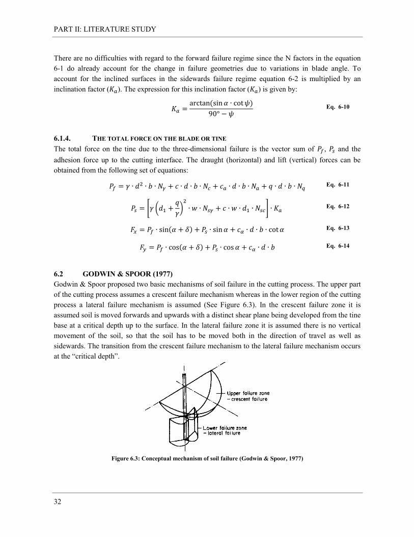
6.2 GODWIN & SPOOR (1977)
Godwin & Spoor proposed two basic mechanisms of soil failure in the cutting process. The upper part
of the cutting process assumes a crescent failure mechanism whereas in the lower region of the cutting
process a lateral failure mechanism is assumed (See Figure 6.3). In the crescent failure zone it is
assumed soil is moved forwards and upwards with a distinct shear plane being developed from the tine
base at a critical depth up to the surface. In the lateral failure zone it is assumed there is no vertical
movement of the soil, so that the soil has to be moved both in the direction of travel as well as
sidewards. The transition from the crescent failure mechanism to the lateral failure mechanism occurs
at the “critical depth”.
Figure 6.3: Conceptual mechanism of soil failure (Godwin & Spoor, 1977)
PART II: LITERATURE STUDY
33
For tines with aspect ratios ( ) larger than unity, the complete soil is failing in crescent failure
whereas for tines with small aspect ratios (< 0.1) the soil is almost completely failing in lateral failure.
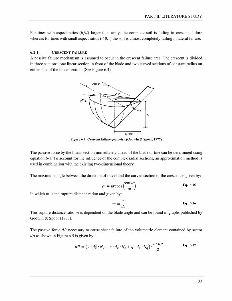
6.2.1. CRESCENT FAILURE
A passive failure mechanism is assumed to occur in the crescent failure area. The crescent is divided
in three sections, one linear section in front of the blade and two curved sections of constant radius on
either side of the linear section. (See Figure 6.4)
Figure 6.4: Crescent failure geometry (Godwin & Spoor, 1977)
The passive force by the linear section immediately ahead of the blade or tine can be determined using
equation 6-1. To account for the influence of the complex radial sections, an approximation method is
used in combination with the existing two-dimensional theory.
The maximum angle between the direction of travel and the curved section of the crescent is given by:
(
) Eq. 6-15
In which is the rupture distance ration and given by:
Eq. 6-16
This rupture distance ratio is dependent on the blade angle and can be found in graphs published by
Godwin & Spoor (1977).
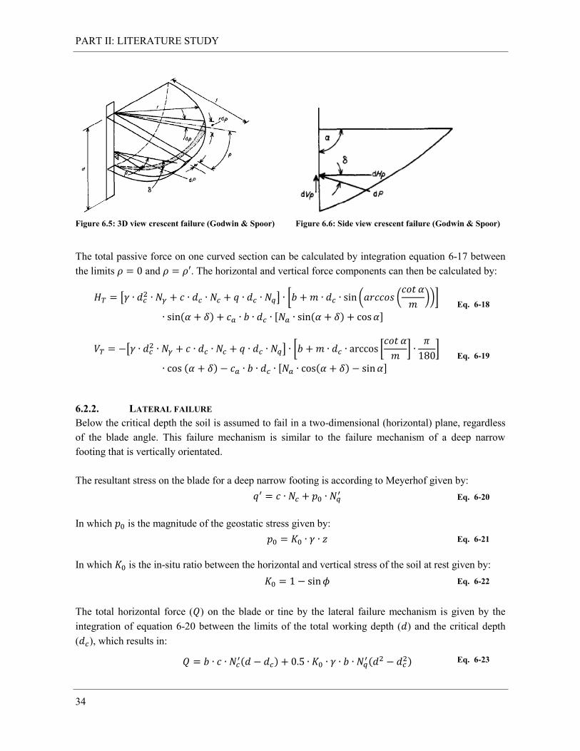
The passive force necessary to cause shear failure of the volumetric element contained by sector
as shown in Figure 6.5 is given by:
( )
Eq. 6-17
PART II: LITERATURE STUDY
34
Figure 6.5: 3D view crescent failure (Godwin & Spoor)
Figure 6.6: Side view crescent failure (Godwin & Spoor)
The total passive force on one curved section can be calculated by integration equation 6-17 between
the limits and . The horizontal and vertical force components can then be calculated by:
[
] [ ( (
))]
( ) [ ( ) ]
Eq. 6-18
[
] [ [
]
]
( ) [ ( ) ] Eq. 6-19
6.2.2. LATERAL FAILURE
Below the critical depth the soil is assumed to fail in a two-dimensional (horizontal) plane, regardless
of the blade angle. This failure mechanism is similar to the failure mechanism of a deep narrow
footing that is vertically orientated.
The resultant stress on the blade for a deep narrow footing is according to Meyerhof given by:
Eq. 6-20
In which is the magnitude of the geostatic stress given by:
Eq. 6-21
In which is the in-situ ratio between the horizontal and vertical stress of the soil at rest given by:
Eq. 6-22
The total horizontal force ( ) on the blade or tine by the lateral failure mechanism is given by the
integration of equation 6-20 between the limits of the total working depth ( ) and the critical depth
( ), which results in:
( )
( ) Eq. 6-23
PART II: LITERATURE STUDY
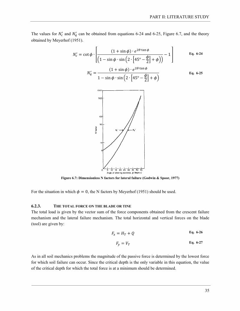
35
The values for and
can be obtained from equations 6-24 and 6-25, Figure 6.7, and the theory
obtained by Meyerhof (1951).
[
( )
( ( [ ] ))
] Eq. 6-24
( )
( [ ] )
Eq. 6-25
Figure 6.7: Dimensionless N factors for lateral failure (Godwin & Spoor, 1977)
For the situation in which , the N factors by Meyerhof (1951) should be used.
6.2.3. THE TOTAL FORCE ON THE BLADE OR TINE
The total load is given by the vector sum of the force components obtained from the crescent failure
mechanism and the lateral failure mechanism. The total horizontal and vertical forces on the blade
(tool) are given by:
Eq. 6-26
Eq. 6-27
As in all soil mechanics problems the magnitude of the passive force is determined by the lowest force
for which soil failure can occur. Since the critical depth is the only variable in this equation, the value
of the critical depth for which the total force is at a minimum should be determined.
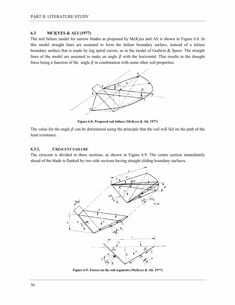
PART II: LITERATURE STUDY
36
6.3 MCKYES & ALI (1977)
The soil failure model for narrow blades as proposed by McKyes and Ali is shown in Figure 6.8. In
this model straight lines are assumed to form the failure boundary surface, instead of a failure
boundary surface that is made by log spiral curves, as in the model of Godwin & Spoor. The straight
lines of the model are assumed to make an angle with the horizontal. This results in the draught
force being a function of the angle in combination with some other soil properties.
Figure 6.8: Proposed soil failure (McKyes & Ali, 1977)
The value for the angle can be determined using the principle that the soil will fail on the path of the
least resistance.
6.3.1. CRESCENT FAILURE
The crescent is divided in three sections, as shown in Figure 6.9. The centre section immediately
ahead of the blade is flanked by two side sections having straight sliding boundary surfaces.
Figure 6.9: Forces on the soil segments (McKyes & Ali, 1977)
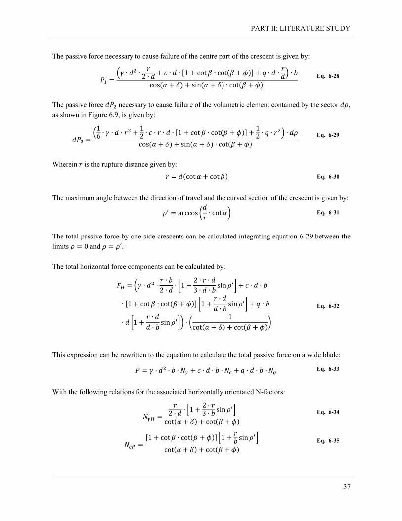
PART II: LITERATURE STUDY
37
The passive force necessary to cause failure of the centre part of the crescent is given by:
(
[ ( )]
)
( ) ( ) ( )
Eq. 6-28
The passive force necessary to cause failure of the volumetric element contained by the sector ,
as shown in Figure 6.9, is given by:
(
[ ( )]
)
( ) ( ) ( )
Eq. 6-29
Wherein is the rupture distance given by:
( ) Eq. 6-30
The maximum angle between the direction of travel and the curved section of the crescent is given by:
(
) Eq. 6-31
The total passive force by one side crescents can be calculated integrating equation 6-29 between the
limits and .
The total horizontal force components can be calculated by:
(
[
]
[ ( )] [
]
[
]) (
( ) ( ))
Eq. 6-32
This expression can be rewritten to the equation to calculate the total passive force on a wide blade:
Eq. 6-33
With the following relations for the associated horizontally orientated N-factors:
[
]
( ) ( )
Eq. 6-34
[ ( )] [
]
( ) ( )
Eq. 6-35

PART II: LITERATURE STUDY
38
[
]
( ) ( )
Eq. 6-36
In these equations the value for is determined such that the value for of the total horizontal forces is
at a minimum.
6.4 GRISSO ET AL. (1980) AND PERUMPRAL ET AL. (1983)
The model of Grisso et al. (1980) and Perumpral et al. (1983) is quite similar to the model developed
by McKyes & Ali. The only difference with this model is that the influence of the side wedges is
replaced by forces acting on the centre. Like in the model of McKyes & Ali the centre wedge is
assumed to have a rupture plane making an angle with the horizontal. Using equilibrium conditions
on the centre wedge, the forces can be written in the Hettiaratchi & Reece earthmoving equation for
wide blades, with exception of the surcharge pressure component :
Eq. 6-37
With the following relations for the N-factors:
[
( ) ( )
( )] Eq. 6-38
[
]
( )
Eq. 6-39
( ) ( )
( )
Eq. 6-40
In which is the height of the soil in front of the tool at failure, , the average depth of the centroid of
the failure wedge, and the area on the side of the failure wedge. These last two can be determined
by:
( ) Eq. 6-41
And
(
) [(
) ] Eq. 6-42
As in all models, failure will occur when the resistance of the soil wedge is at a minimum (
).
PART II: LITERATURE STUDY
39
The total draught (horizontal) and lift (vertical) forces can be calculated by:
( ) Eq. 6-43
( ) Eq. 6-44
6.5 ADVANTAGES AND DISADVANTAGES OF THE NARROW TINE MODELS
Hettiaratchi & Reece (1967) can be used without prior knowledge of the rupture distance. It can be
used for blade angles between 20° < < 160°, and calculation of the required draught and lift forces is
very straight forward. The model is known to overestimate the required forces for vertical blades,
whereas for inclined blades the model is known to underestimate these forces.
Godwin & Spoor (1977) requires prior knowledge of the rupture distance or a model predicting
rupture distance ratios. The graph for predicting the rupture distance ratio as given in Godwin & Spoor
(1977) is usable for blade angles up to 90 degrees. For larger angles up to 160 degrees, the graph as
proposed by Hettiaratchi & Reece (1966) can be to predict the rupture distance ratio.
McKyes & Ali (1977) require prior knowledge of the rupture distance ratio as the model dictates a
certain failure shape based on a combination of blade geometry and soil properties. The draught force
is a function of the angle which can be defined using the principle the total force function is
minimised with respect to this angle. The paper by McKyes & Ali (1977) describes a one wedge
model as well as a two wedge model. For comparison with the other narrow tine theories only the one
wedge model is reviewed. In general, the values predicted by the two wedge model are a bit lower
than the values predicted by the one wedge model. The model can predict the required draught force
for blade angles up to 90° but is unable to predict the associated lift force.
The model of Grisso et al (1980) and Perumpral et al. (1983) can be used for blade angles up to 90
degrees. The resulting equation for the passive earth force as proposed in this theory is a function of
the angle . This angle can be defined using the principle the total passive earth force is minimised
with respect to this angle.
The narrow tine models do not account for the influence of the ploughing velocity on the required
draught forces. In addition, the models do not account for the friction or adhesion along the sides of
the tine, which means the models are only predicting the force required to cut the soil in front of the
tool.
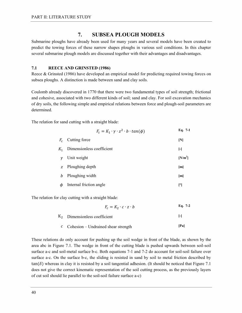
PART II: LITERATURE STUDY
40
7. SUBSEA PLOUGH MODELS
Submarine ploughs have already been used for many years and several models have been created to
predict the towing forces of these narrow shapes ploughs in various soil conditions. In this chapter
several submarine plough models are discussed together with their advantages and disadvantages.
7.1 REECE AND GRINSTED (1986)
Reece & Grinsted (1986) have developed an empirical model for predicting required towing forces on
subsea ploughs. A distinction is made between sand and clay soils.
Coulomb already discovered in 1770 that there were two fundamental types of soil strength; frictional
and cohesive, associated with two different kinds of soil; sand and clay. For soil excavation mechanics
of dry soils, the following simple and empirical relations between force and plough-soil parameters are
determined.
The relation for sand cutting with a straight blade:
( ) Eq. 7-1
Cutting force [N]
Dimensionless coefficient [-]
Unit weight [N/m3]
Ploughing depth [m]
Ploughing width [m]
Internal friction angle [°]
The relation for clay cutting with a straight blade:
Eq. 7-2
Dimensionless coefficient [-]
Cohesion – Undrained shear strength [Pa]
These relations do only account for pushing up the soil wedge in front of the blade, as shown by the
area abc in Figure 7.1. The wedge in front of the cutting blade is pushed upwards between soil-soil
surface a-c and soil-metal surface b-c. Both equations 7-1 and 7-2 do account for soil-soil failure over
surface a-c. On the surface b-c, the sliding is resisted in sand by soil to metal friction described by
( ) whereas in clay it is resisted by a soil tangential adhesion. (It should be noticed that Figure 7.1
does not give the correct kinematic representation of the soil cutting process, as the previously layers
of cut soil should lie parallel to the soil-soil failure surface a-c)
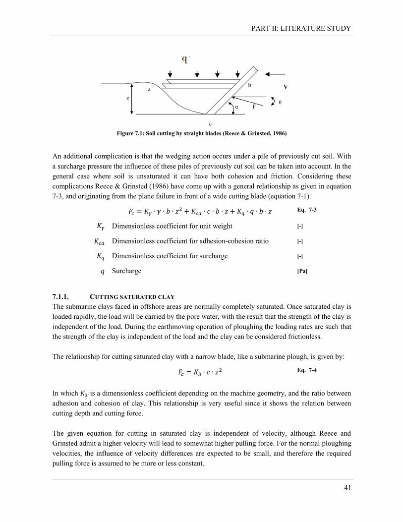
PART II: LITERATURE STUDY
41
Figure 7.1: Soil cutting by straight blades (Reece & Grinsted, 1986)
An additional complication is that the wedging action occurs under a pile of previously cut soil. With
a surcharge pressure the influence of these piles of previously cut soil can be taken into account. In the
general case where soil is unsaturated it can have both cohesion and friction. Considering these
complications Reece & Grinsted (1986) have come up with a general relationship as given in equation
7-3, and originating from the plane failure in front of a wide cutting blade (equation 7-1).
Eq. 7-3
Dimensionless coefficient for unit weight [-]
Dimensionless coefficient for adhesion-cohesion ratio [-]
Dimensionless coefficient for surcharge [-]
Surcharge [Pa]
7.1.1. CUTTING SATURATED CLAY
The submarine clays faced in offshore areas are normally completely saturated. Once saturated clay is
loaded rapidly, the load will be carried by the pore water, with the result that the strength of the clay is
independent of the load. During the earthmoving operation of ploughing the loading rates are such that
the strength of the clay is independent of the load and the clay can be considered frictionless.
The relationship for cutting saturated clay with a narrow blade, like a submarine plough, is given by:
Eq. 7-4
In which is a dimensionless coefficient depending on the machine geometry, and the ratio between
adhesion and cohesion of clay. This relationship is very useful since it shows the relation between
cutting depth and cutting force.
The given equation for cutting in saturated clay is independent of velocity, although Reece and
Grinsted admit a higher velocity will lead to somewhat higher pulling force. For the normal ploughing
velocities, the influence of velocity differences are expected to be small, and therefore the required
pulling force is assumed to be more or less constant.
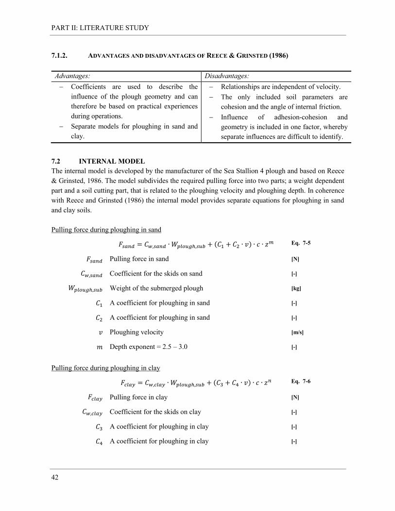
PART II: LITERATURE STUDY
42
7.1.2. ADVANTAGES AND DISADVANTAGES OF REECE & GRINSTED (1986)
Advantages: Disadvantages:
Coefficients are used to describe the
influence of the plough geometry and can
therefore be based on practical experiences
during operations.
Separate models for ploughing in sand and
clay.
Relationships are independent of velocity.
The only included soil parameters are
cohesion and the angle of internal friction.
Influence of adhesion-cohesion and
geometry is included in one factor, whereby
separate influences are difficult to identify.
7.2 INTERNAL MODEL
The internal model is developed by the manufacturer of the Sea Stallion 4 plough and based on Reece
& Grinsted, 1986. The model subdivides the required pulling force into two parts; a weight dependent
part and a soil cutting part, that is related to the ploughing velocity and ploughing depth. In coherence
with Reece and Grinsted (1986) the internal model provides separate equations for ploughing in sand
and clay soils.
Pulling force during ploughing in sand
( ) Eq. 7-5
Pulling force in sand [N]
Coefficient for the skids on sand [-]
Weight of the submerged plough [kg]
A coefficient for ploughing in sand [-]
A coefficient for ploughing in sand [-]
Ploughing velocity [m/s]
Depth exponent = 2.5 – 3.0 [-]
Pulling force during ploughing in clay
( ) Eq. 7-6
Pulling force in clay [N]
Coefficient for the skids on clay [-]
A coefficient for ploughing in clay [-]
A coefficient for ploughing in clay [-]
PART II: LITERATURE STUDY
43
Depth exponent = 1.5 – 2.0 [-]
Coefficients depend on the plough type, its specific interaction with soil and
characteristics of the soil. When sufficient data is gathered for a specific plough geometry in various
soil conditions and with various ploughing velocities coefficients can be estimated using a curve
fitting method.
7.2.1. ADVANTAGES AND DISADVANTAGES OF THE INTERNAL MODEL
Since this model is based on the theory of Reece and Grinsted it has many advantages and
disadvantages in common.
Advantages: Disadvantages:
Simple relations.
Coefficients are used to describe the
influence of the plough geometry in
different soils, which can be based on
practical experiences during operations.
Relationships that are velocity dependent.
Separate models for ploughing in sand and
clay.
Highly empirical.
Untransparent, all parameters are caught
in one coefficient, whereby individual
influences of geometries and soil
parameters are difficult to identify.
Coefficients dependent on soil type,
which requires different coefficients for
all different soil types.
PART II: LITERATURE STUDY
44
7.3 ADDITIONAL ADHESION
Extra friction terms can be added to the ultimate bearing capacity theory in order to develop a
complete force prediction model for the Sea Stallion 4 plough. Separate models are developed to
calculate the extra friction or adhesion along the skids, heel and share in sand and clay soil conditions.
7.3.1. ADDITIONAL FRICTION IN SAND
The friction on the skids can be calculated by:
( ) Eq. 7-7
The additional force on the skids in sand [N]
Angle of external friction [°]
Vertical load [N]
The friction on the share depends on the load perpendicular to the share, which in turn is depending on
the average soil stress and the side area of the share. The friction along the share can be calculated by:
( ) ( )
( )
Eq. 7-8
The additional force on the share in sand [N]
Side area of the share [m2]
Submerged soil density [kg/m3]
7.3.2. ADDITIONAL ADHESION IN CLAY
Adhesion will appear along the share, skids and heel during ploughing in clay soil conditions due to
adhesion between the steel-clay surfaces. The adhesion generated by the skids, share and heel can be
calculated by:
Eq. 7-9
Eq. 7-10
Eq. 7-11
The additional force on the skids, share and heel in clay [N]
Adhesion [Pa]
Area of the skids, share and heel [m2]
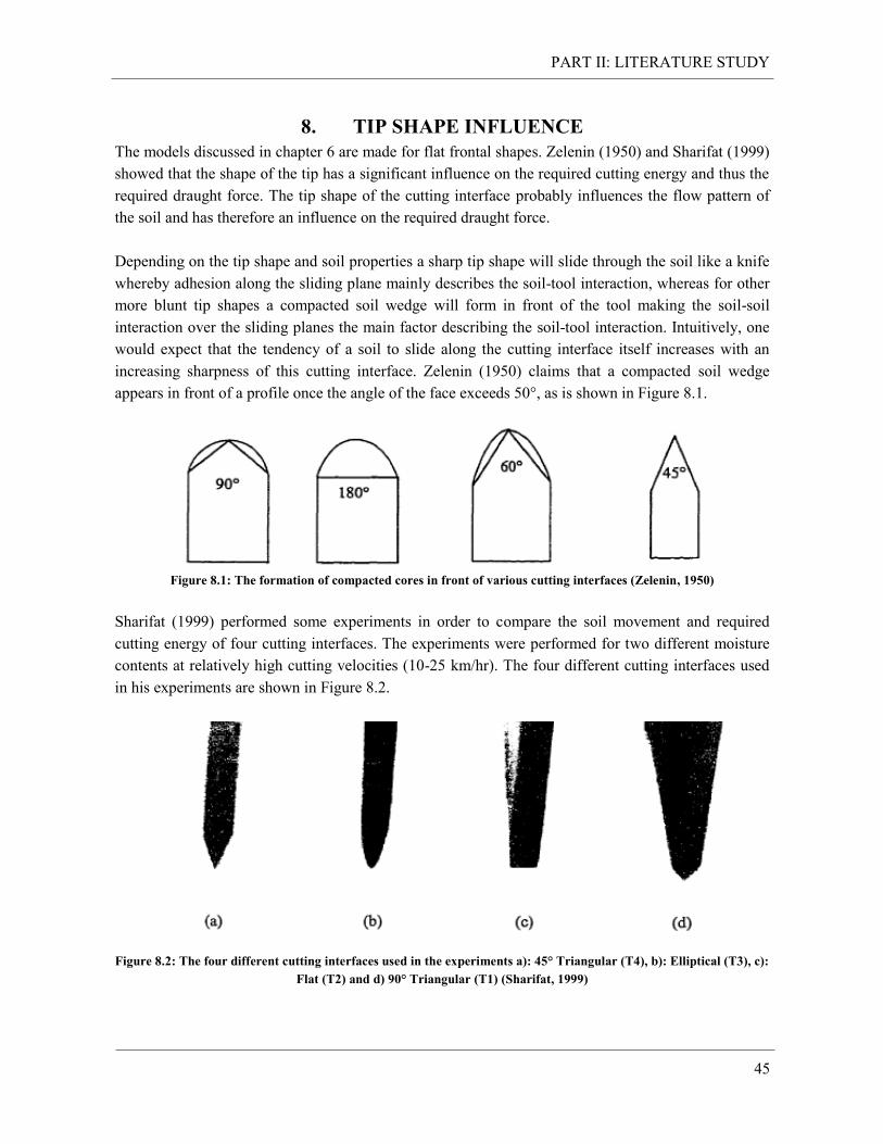
PART II: LITERATURE STUDY
45
8. TIP SHAPE INFLUENCE
The models discussed in chapter 6 are made for flat frontal shapes. Zelenin (1950) and Sharifat (1999)
showed that the shape of the tip has a significant influence on the required cutting energy and thus the
required draught force. The tip shape of the cutting interface probably influences the flow pattern of
the soil and has therefore an influence on the required draught force.
Depending on the tip shape and soil properties a sharp tip shape will slide through the soil like a knife
whereby adhesion along the sliding plane mainly describes the soil-tool interaction, whereas for other
more blunt tip shapes a compacted soil wedge will form in front of the tool making the soil-soil
interaction over the sliding planes the main factor describing the soil-tool interaction. Intuitively, one
would expect that the tendency of a soil to slide along the cutting interface itself increases with an
increasing sharpness of this cutting interface. Zelenin (1950) claims that a compacted soil wedge
appears in front of a profile once the angle of the face exceeds 50°, as is shown in Figure 8.1.
Figure 8.1: The formation of compacted cores in front of various cutting interfaces (Zelenin, 1950)
Sharifat (1999) performed some experiments in order to compare the soil movement and required
cutting energy of four cutting interfaces. The experiments were performed for two different moisture
contents at relatively high cutting velocities (10-25 km/hr). The four different cutting interfaces used
in his experiments are shown in Figure 8.2.
Figure 8.2: The four different cutting interfaces used in the experiments a): 45° Triangular (T4), b): Elliptical (T3), c):
Flat (T2) and d) 90° Triangular (T1) (Sharifat, 1999)
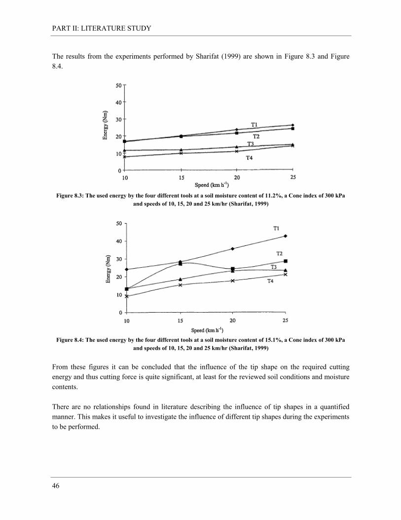
PART II: LITERATURE STUDY
46
The results from the experiments performed by Sharifat (1999) are shown in Figure 8.3 and Figure
8.4.
Figure 8.3: The used energy by the four different tools at a soil moisture content of 11.2%, a Cone index of 300 kPa
and speeds of 10, 15, 20 and 25 km/hr (Sharifat, 1999)
Figure 8.4: The used energy by the four different tools at a soil moisture content of 15.1%, a Cone index of 300 kPa
and speeds of 10, 15, 20 and 25 km/hr (Sharifat, 1999)
From these figures it can be concluded that the influence of the tip shape on the required cutting
energy and thus cutting force is quite significant, at least for the reviewed soil conditions and moisture
contents.
There are no relationships found in literature describing the influence of tip shapes in a quantified
manner. This makes it useful to investigate the influence of different tip shapes during the experiments
to be performed.
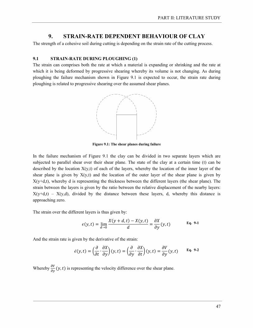
PART II: LITERATURE STUDY
47
9. STRAIN-RATE DEPENDENT BEHAVIOUR OF CLAY
The strength of a cohesive soil during cutting is depending on the strain rate of the cutting process.
9.1 STRAIN-RATE DURING PLOUGHING (1)
The strain can comprises both the rate at which a material is expanding or shrinking and the rate at
which it is being deformed by progressive shearing whereby its volume is not changing. As during
ploughing the failure mechanism shown in Figure 9.1 is expected to occur, the strain rate during
ploughing is related to progressive shearing over the assumed shear planes.
Figure 9.1: The shear planes during failure
In the failure mechanism of Figure 9.1 the clay can be divided in two separate layers which are
subjected to parallel shear over their shear plane. The state of the clay at a certain time (t) can be
described by the location X(y,t) of each of the layers, whereby the location of the inner layer of the
shear plane is given by X(y,t) and the location of the outer layer of the shear plane is given by
X(y+d,t), whereby d is representing the thickness between the different layers (the shear plane). The
strain between the layers is given by the ratio between the relative displacement of the nearby layers:
X(y+d,t) – X(y,d), divided by the distance between these layers, d, whereby this distance is
approaching zero.
The strain over the different layers is thus given by:
( )
( ) ( )
( ) Eq. 9-1
And the strain rate is given by the derivative of the strain:
( ) (
) ( ) (
) ( )
( ) Eq. 9-2
Whereby
( ) is representing the velocity difference over the shear plane.
PART II: LITERATURE STUDY
48
9.2 INFLUENCE OF THE VELOCITY ON THE UNDRAINED SHEAR STRENGTH
Various researchers have tried to make models to describe the strain rate dependent behaviour of clay.
Most of these models are rather similar and relate the undrained shear strength at a certain strain rate
to the undrained shear strength at a reference strain rate , using an exponential or logarithmic
function. For the failure mechanisms expected during ploughing in clay soils the strain rate is equal to
the velocity difference over the shear planes. Since the velocity difference over the shear planes is
directly related to the forward velocity of the plough, the strain rates as used in the equations found in
literature can be replaced by the ploughing velocities.
In general the increase in the undrained shear strength by increasing ploughing velocities is large
compared to the increase of the inertial force by this same velocity increase. The strain-rate
dependency relations are only valid above a certain velocity, which is in the order of 0.5-1 mm/s. The
exponential model proposed by various researchers is given by:
[
]
Eq. 9-3
According to Wismer & Luth (1972) with values ranging from 0.091 to 0.109. This exponential
model is quite similar to the logarithmic model that is proposed by other researchers, and which is
given by:
( [
]) Eq. 9-4
According to Dayal & Allen (1975) with values ranging from 0.03 to 0.25. As the velocities come
close to zero, the exponential model will result in values for close to zero whereas the logarithmic
model will result in negative values for . The logarithmic model is thus giving incorrect values for
low velocities.
In order to exclude the incorrect behaviour at low velocities from the exponential and logarithmic
strain rate dependency models, Miedema (1992) derived a more correct model. This model is based on
the exponential and logarithmic relations but allows for a yield stress (adhesion and/or cohesion) for a
material at rest. The model developed by Miedema (1992) is given by:
(
[
]) Eq. 9-5
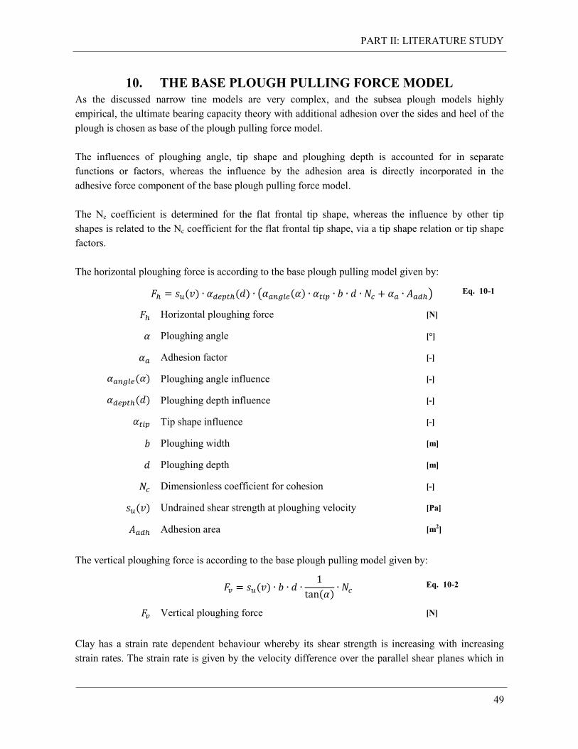
PART II: LITERATURE STUDY
49
10. THE BASE PLOUGH PULLING FORCE MODEL
As the discussed narrow tine models are very complex, and the subsea plough models highly
empirical, the ultimate bearing capacity theory with additional adhesion over the sides and heel of the
plough is chosen as base of the plough pulling force model.
The influences of ploughing angle, tip shape and ploughing depth is accounted for in separate
functions or factors, whereas the influence by the adhesion area is directly incorporated in the
adhesive force component of the base plough pulling force model.
The Nc coefficient is determined for the flat frontal tip shape, whereas the influence by other tip
shapes is related to the Nc coefficient for the flat frontal tip shape, via a tip shape relation or tip shape
factors.
The horizontal ploughing force is according to the base plough pulling model given by:
( ) ( ) ( ( ) ) Eq. 10-1
Horizontal ploughing force [N]
Ploughing angle [°]
Adhesion factor [-]
( ) Ploughing angle influence [-]
( ) Ploughing depth influence [-]
Tip shape influence [-]
Ploughing width [m]
Ploughing depth [m]
Dimensionless coefficient for cohesion [-]
( ) Undrained shear strength at ploughing velocity [Pa]
Adhesion area [m2]
The vertical ploughing force is according to the base plough pulling model given by:
( )
( ) Eq. 10-2
Vertical ploughing force [N]
Clay has a strain rate dependent behaviour whereby its shear strength is increasing with increasing
strain rates. The strain rate is given by the velocity difference over the parallel shear planes which in
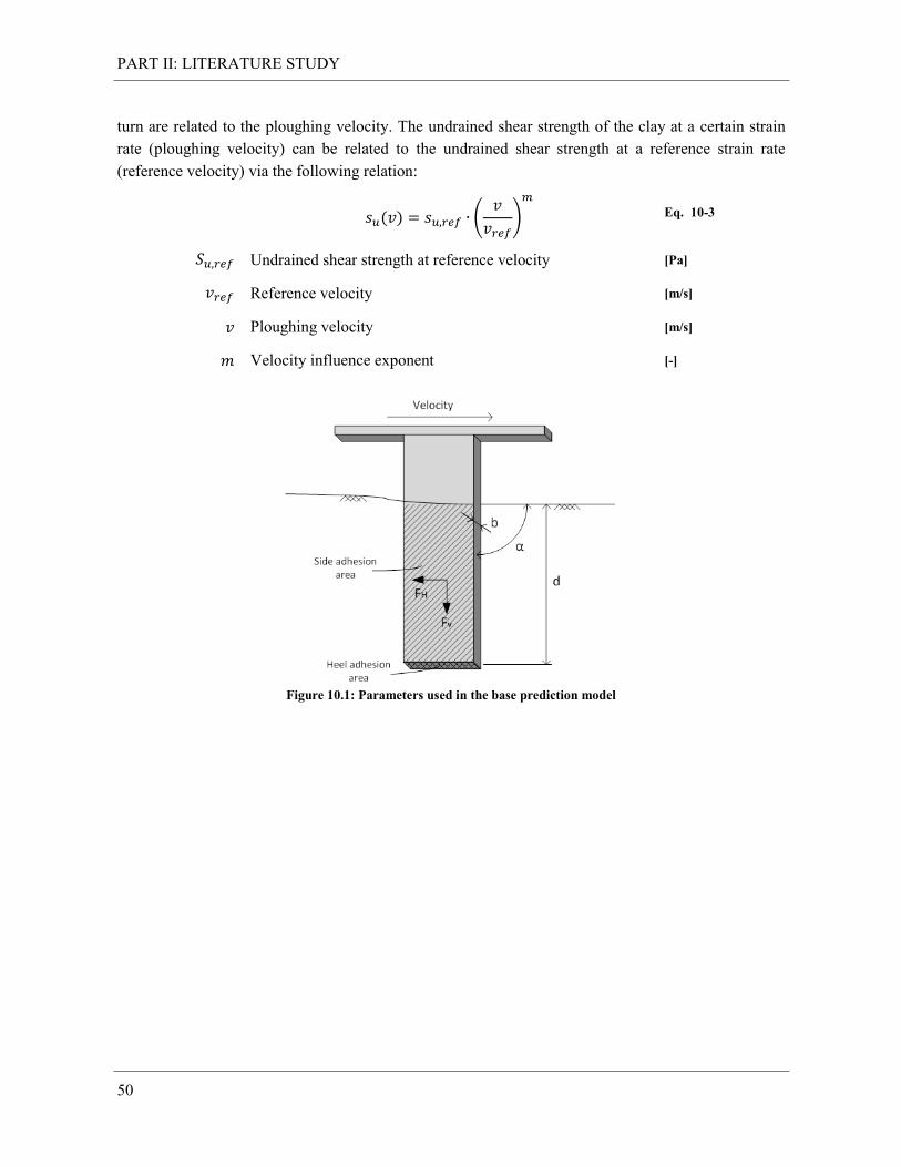
PART II: LITERATURE STUDY
50
turn are related to the ploughing velocity. The undrained shear strength of the clay at a certain strain
rate (ploughing velocity) can be related to the undrained shear strength at a reference strain rate
(reference velocity) via the following relation:
( ) (
)
Eq. 10-3
Undrained shear strength at reference velocity [Pa]
Reference velocity [m/s]
Ploughing velocity [m/s]
Velocity influence exponent [-]
Figure 10.1: Parameters used in the base prediction model

PART III: THE PRELIMINARY EXPERIMENTS
51
PART III: THE PRELIMINARY EXPERIMENTS
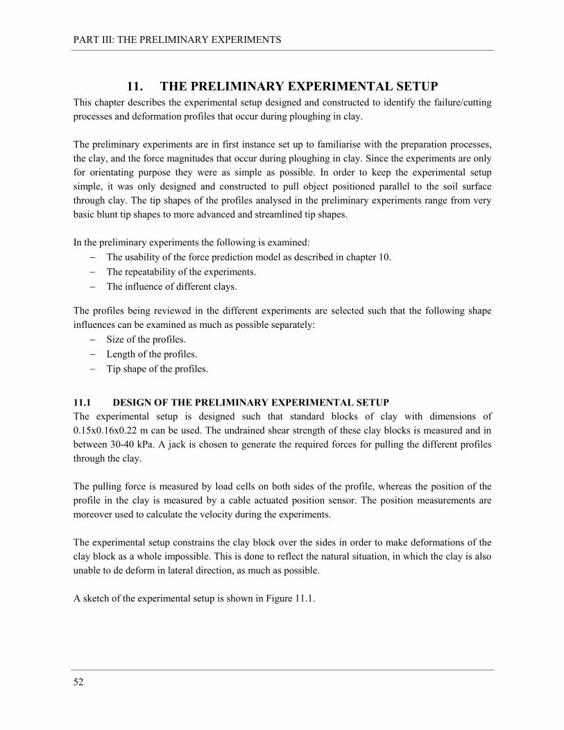
PART III: THE PRELIMINARY EXPERIMENTS
52
11. THE PRELIMINARY EXPERIMENTAL SETUP
This chapter describes the experimental setup designed and constructed to identify the failure/cutting
processes and deformation profiles that occur during ploughing in clay.
The preliminary experiments are in first instance set up to familiarise with the preparation processes,
the clay, and the force magnitudes that occur during ploughing in clay. Since the experiments are only
for orientating purpose they were as simple as possible. In order to keep the experimental setup
simple, it was only designed and constructed to pull object positioned parallel to the soil surface
through clay. The tip shapes of the profiles analysed in the preliminary experiments range from very
basic blunt tip shapes to more advanced and streamlined tip shapes.
In the preliminary experiments the following is examined:
The usability of the force prediction model as described in chapter 10.
The repeatability of the experiments.
The influence of different clays.
The profiles being reviewed in the different experiments are selected such that the following shape
influences can be examined as much as possible separately:
Size of the profiles.
Length of the profiles.
Tip shape of the profiles.
11.1 DESIGN OF THE PRELIMINARY EXPERIMENTAL SETUP
The experimental setup is designed such that standard blocks of clay with dimensions of
0.15x0.16x0.22 m can be used. The undrained shear strength of these clay blocks is measured and in
between 30-40 kPa. A jack is chosen to generate the required forces for pulling the different profiles
through the clay.
The pulling force is measured by load cells on both sides of the profile, whereas the position of the
profile in the clay is measured by a cable actuated position sensor. The position measurements are
moreover used to calculate the velocity during the experiments.
The experimental setup constrains the clay block over the sides in order to make deformations of the
clay block as a whole impossible. This is done to reflect the natural situation, in which the clay is also
unable to de deform in lateral direction, as much as possible.
A sketch of the experimental setup is shown in Figure 11.1.
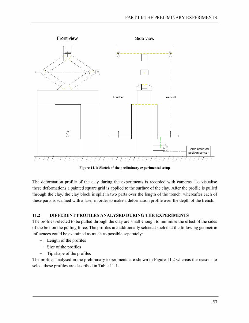
PART III: THE PRELIMINARY EXPERIMENTS
53
Figure 11.1: Sketch of the preliminary experimental setup
The deformation profile of the clay during the experiments is recorded with cameras. To visualise
these deformations a painted square grid is applied to the surface of the clay. After the profile is pulled
through the clay, the clay block is split in two parts over the length of the trench, whereafter each of
these parts is scanned with a laser in order to make a deformation profile over the depth of the trench.
11.2 DIFFERENT PROFILES ANALYSED DURING THE EXPERIMENTS
The profiles selected to be pulled through the clay are small enough to minimise the effect of the sides
of the box on the pulling force. The profiles are additionally selected such that the following geometric
influences could be examined as much as possible separately:
Length of the profiles
Size of the profiles
Tip shape of the profiles
The profiles analysed in the preliminary experiments are shown in Figure 11.2 whereas the reasons to
select these profiles are described in Table 11-1.
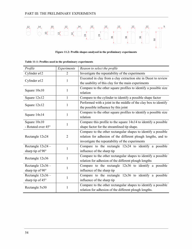
PART III: THE PRELIMINARY EXPERIMENTS
54
Figure 11.2: Profile shapes analysed in the preliminary experiments
Table 11-1: Profiles used in the preliminary experiments
Profile Experiments Reason to select the profile
Cylinder ø12 2 Investigate the repeatability of the experiments
Cylinder ø12 1 Executed in clay from a clay extraction site in Deest to review
the usability of this clay for the main experiments
Square 10x10 1 Compare to the other square profiles to identify a possible size
relation
Square 12x12 1 Compare to the cylinder to identify a possible shape factor
Square 12x12 1 Performed with a joint in the middle of the clay box to identify
the possible influence by this joint
Square 14x14 1 Compare to the other square profiles to identify a possible size
relation
Square 10x10
- Rotated over 45° 1
Compare this profile to the square 14x14 to identify a possible
shape factor for the streamlined tip shape.
Rectangle 12x24 2
Compare to the other rectangular shapes to identify a possible
relation for adhesion of the different plough lengths, and to
investigate the repeatability of the experiments
Rectangle 12x24 –
sharp tip of 90° 1
Compare to the rectangle 12x24 to identify a possible
influence of the sharp tip
Rectangle 12x36 1 Compare to the other rectangular shapes to identify a possible
relation for adhesion of the different plough lengths
Rectangle 12x36 –
sharp tip of 90° 1
Compare to the rectangle 12x36 to identify a possible
influence of the sharp tip
Rectangle 12x36 –
sharp tip of 45° 1
Compare to the rectangle 12x36 to identify a possible
influence of the sharp tip
Rectangle 5x50 1 Compare to the other rectangular shapes to identify a possible
relation for adhesion of the different plough lengths.
12 12 12
12
24
12
36
5
50
14
1410
10
12
24
12
36
14 12
36
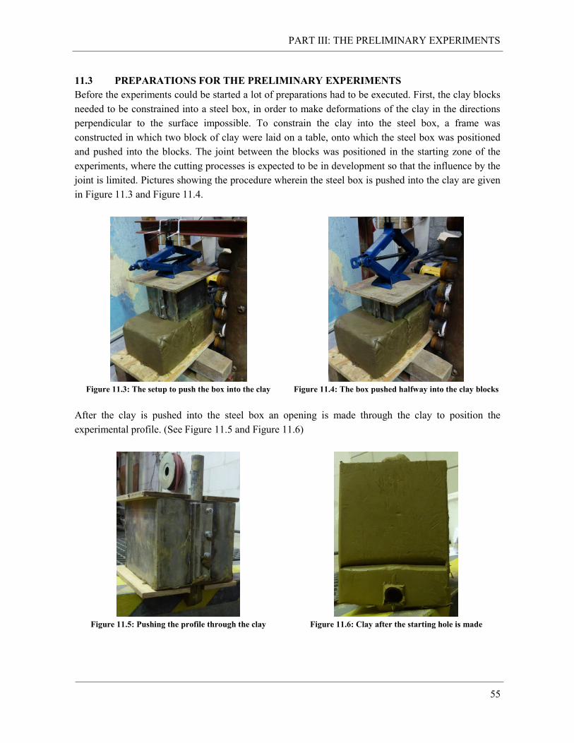
PART III: THE PRELIMINARY EXPERIMENTS
55
11.3 PREPARATIONS FOR THE PRELIMINARY EXPERIMENTS
Before the experiments could be started a lot of preparations had to be executed. First, the clay blocks
needed to be constrained into a steel box, in order to make deformations of the clay in the directions
perpendicular to the surface impossible. To constrain the clay into the steel box, a frame was
constructed in which two block of clay were laid on a table, onto which the steel box was positioned
and pushed into the blocks. The joint between the blocks was positioned in the starting zone of the
experiments, where the cutting processes is expected to be in development so that the influence by the
joint is limited. Pictures showing the procedure wherein the steel box is pushed into the clay are given
in Figure 11.3 and Figure 11.4.
Figure 11.3: The setup to push the box into the clay
Figure 11.4: The box pushed halfway into the clay blocks
After the clay is pushed into the steel box an opening is made through the clay to position the
experimental profile. (See Figure 11.5 and Figure 11.6)
Figure 11.5: Pushing the profile through the clay
Figure 11.6: Clay after the starting hole is made
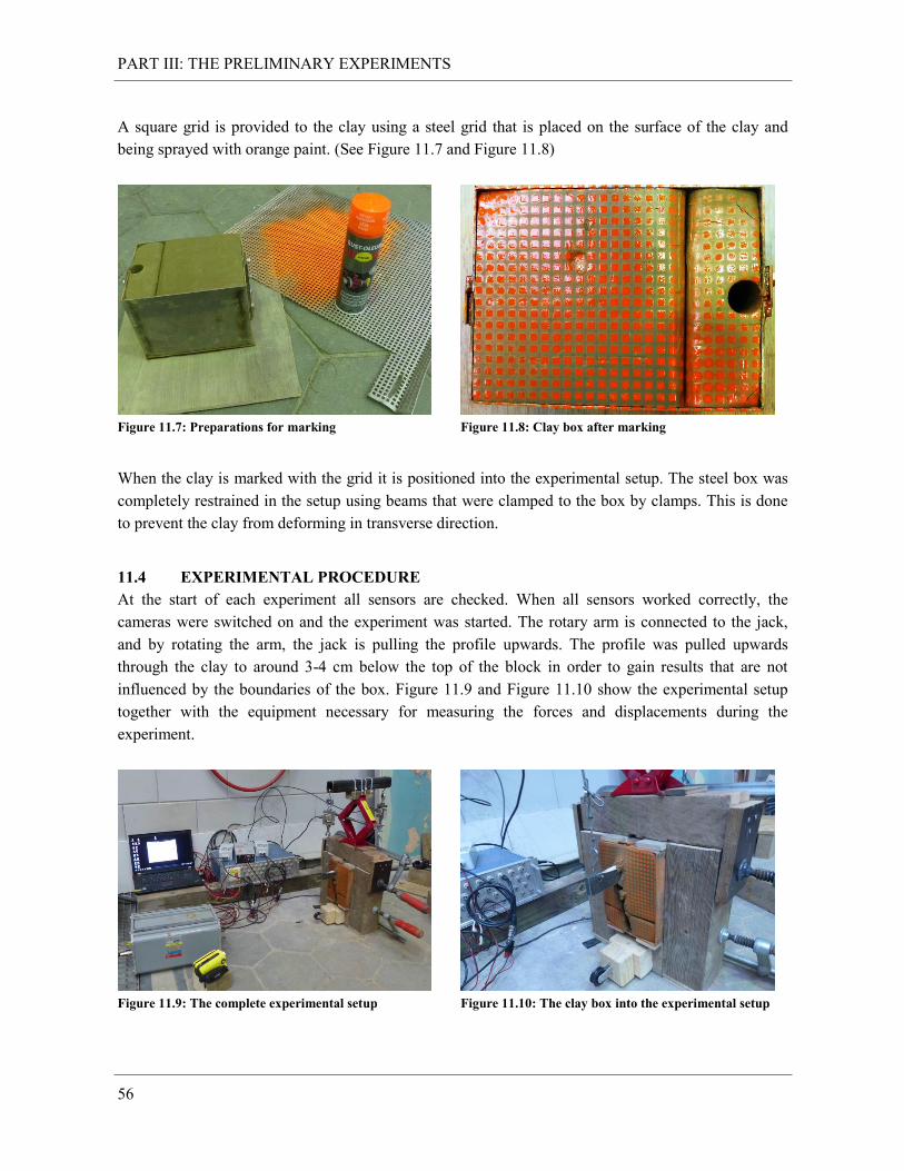
PART III: THE PRELIMINARY EXPERIMENTS
56
A square grid is provided to the clay using a steel grid that is placed on the surface of the clay and
being sprayed with orange paint. (See Figure 11.7 and Figure 11.8)
Figure 11.7: Preparations for marking
Figure 11.8: Clay box after marking
When the clay is marked with the grid it is positioned into the experimental setup. The steel box was
completely restrained in the setup using beams that were clamped to the box by clamps. This is done
to prevent the clay from deforming in transverse direction.
11.4 EXPERIMENTAL PROCEDURE
At the start of each experiment all sensors are checked. When all sensors worked correctly, the
cameras were switched on and the experiment was started. The rotary arm is connected to the jack,
and by rotating the arm, the jack is pulling the profile upwards. The profile was pulled upwards
through the clay to around 3-4 cm below the top of the block in order to gain results that are not
influenced by the boundaries of the box. Figure 11.9 and Figure 11.10 show the experimental setup
together with the equipment necessary for measuring the forces and displacements during the
experiment.
Figure 11.9: The complete experimental setup
Figure 11.10: The clay box into the experimental setup
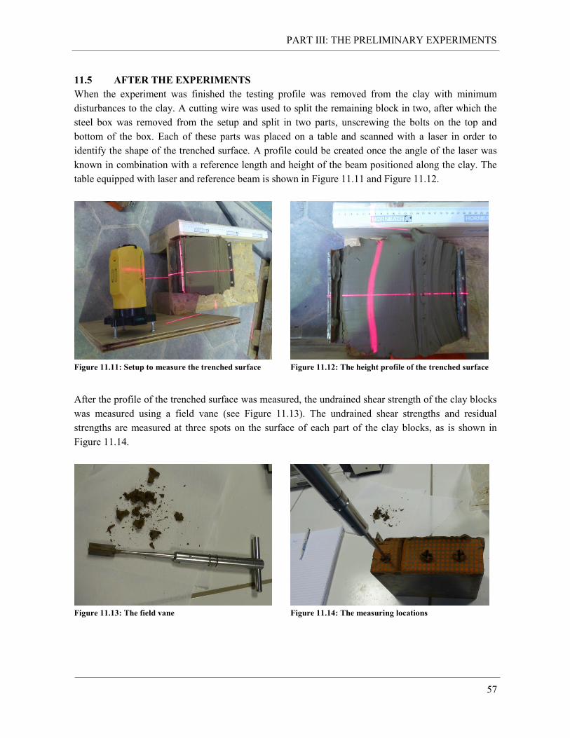
PART III: THE PRELIMINARY EXPERIMENTS
57
11.5 AFTER THE EXPERIMENTS
When the experiment was finished the testing profile was removed from the clay with minimum
disturbances to the clay. A cutting wire was used to split the remaining block in two, after which the
steel box was removed from the setup and split in two parts, unscrewing the bolts on the top and
bottom of the box. Each of these parts was placed on a table and scanned with a laser in order to
identify the shape of the trenched surface. A profile could be created once the angle of the laser was
known in combination with a reference length and height of the beam positioned along the clay. The
table equipped with laser and reference beam is shown in Figure 11.11 and Figure 11.12.
Figure 11.11: Setup to measure the trenched surface
Figure 11.12: The height profile of the trenched surface
After the profile of the trenched surface was measured, the undrained shear strength of the clay blocks
was measured using a field vane (see Figure 11.13). The undrained shear strengths and residual
strengths are measured at three spots on the surface of each part of the clay blocks, as is shown in
Figure 11.14.
Figure 11.13: The field vane
Figure 11.14: The measuring locations
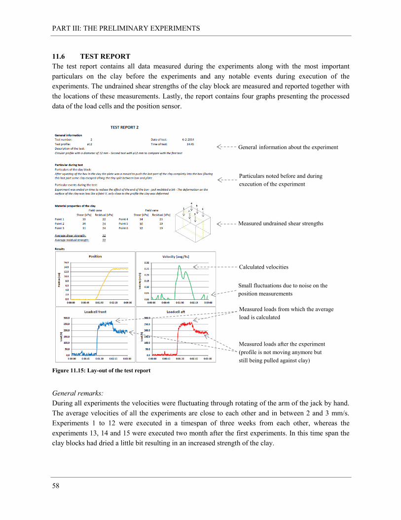
PART III: THE PRELIMINARY EXPERIMENTS
58
11.6 TEST REPORT
The test report contains all data measured during the experiments along with the most important
particulars on the clay before the experiments and any notable events during execution of the
experiments. The undrained shear strengths of the clay block are measured and reported together with
the locations of these measurements. Lastly, the report contains four graphs presenting the processed
data of the load cells and the position sensor.
Figure 11.15: Lay-out of the test report
General remarks:
During all experiments the velocities were fluctuating through rotating of the arm of the jack by hand.
The average velocities of all the experiments are close to each other and in between 2 and 3 mm/s.
Experiments 1 to 12 were executed in a timespan of three weeks from each other, whereas the
experiments 13, 14 and 15 were executed two month after the first experiments. In this time span the
clay blocks had dried a little bit resulting in an increased strength of the clay.
General information about the experiment
Particulars noted before and during
execution of the experiment
Calculated velocities
Measured loads from which the average
load is calculated
Measured loads after the experiment
(profile is not moving anymore but
still being pulled against clay)
Measured undrained shear strengths
Small fluctuations due to noise on the
position measurements
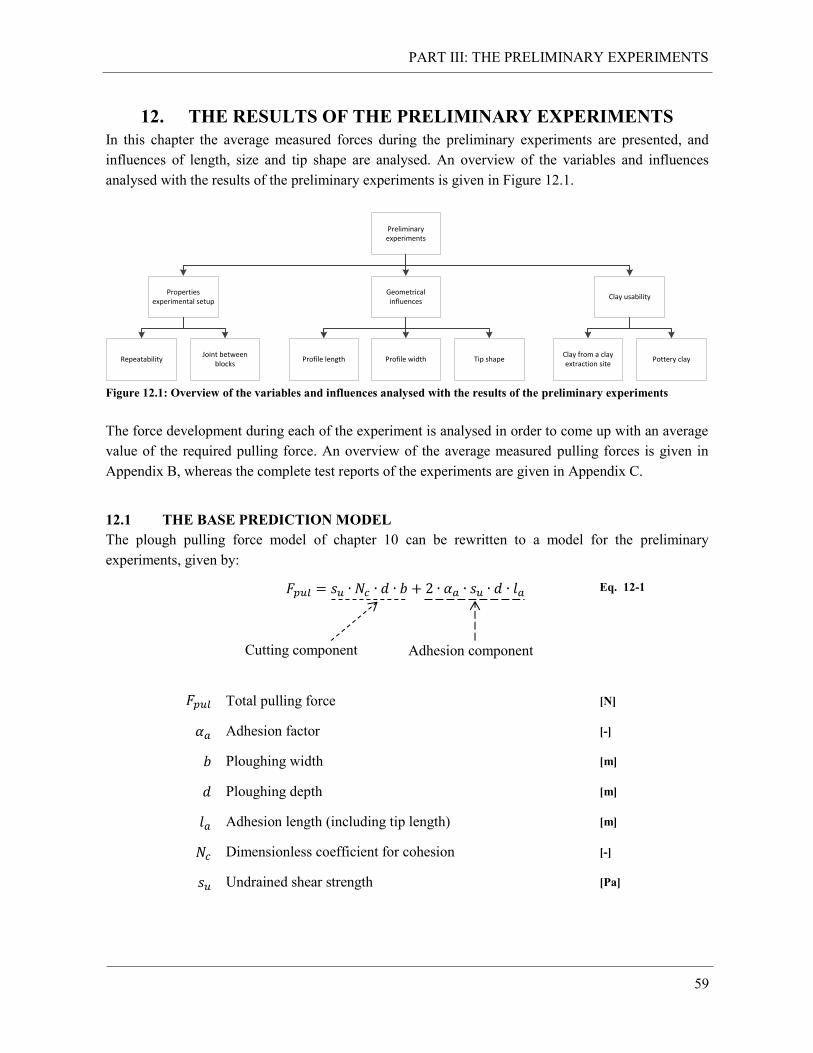
PART III: THE PRELIMINARY EXPERIMENTS
59
12. THE RESULTS OF THE PRELIMINARY EXPERIMENTS
In this chapter the average measured forces during the preliminary experiments are presented, and
influences of length, size and tip shape are analysed. An overview of the variables and influences
analysed with the results of the preliminary experiments is given in Figure 12.1.
Figure 12.1: Overview of the variables and influences analysed with the results of the preliminary experiments
The force development during each of the experiment is analysed in order to come up with an average
value of the required pulling force. An overview of the average measured pulling forces is given in
Appendix B, whereas the complete test reports of the experiments are given in Appendix C.
12.1 THE BASE PREDICTION MODEL
The plough pulling force model of chapter 10 can be rewritten to a model for the preliminary
experiments, given by:
Eq. 12-1
Total pulling force [N]
Adhesion factor [-]
Ploughing width [m]
Ploughing depth [m]
Adhesion length (including tip length) [m]
Dimensionless coefficient for cohesion [-]
Undrained shear strength [Pa]
Preliminary experiments
Clay usabilityGeometrical influences
Properties experimental setup
RepeatabilityJoint between
blocksProfile length Profile width Tip shape Pottery clay
Clay from a clay extraction site
Cutting component Adhesion component
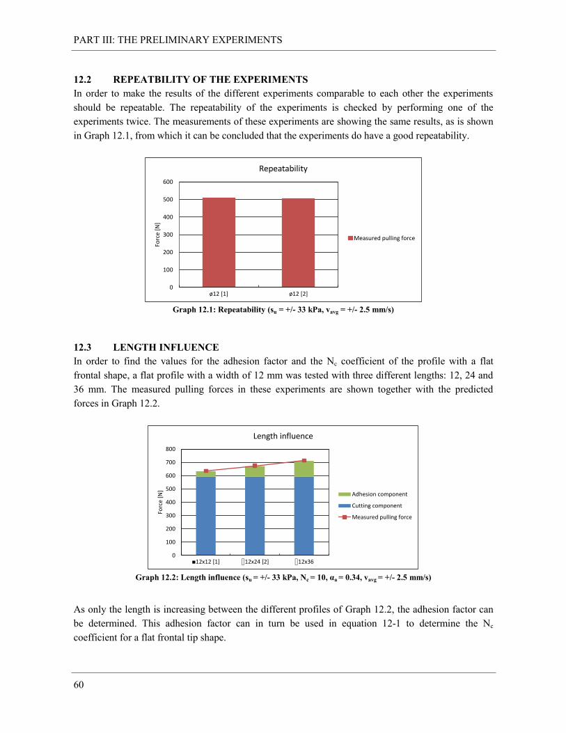
PART III: THE PRELIMINARY EXPERIMENTS
60
12.2 REPEATBILITY OF THE EXPERIMENTS
In order to make the results of the different experiments comparable to each other the experiments
should be repeatable. The repeatability of the experiments is checked by performing one of the
experiments twice. The measurements of these experiments are showing the same results, as is shown
in Graph 12.1, from which it can be concluded that the experiments do have a good repeatability.
Graph 12.1: Repeatability (su = +/- 33 kPa, vavg = +/- 2.5 mm/s)
12.3 LENGTH INFLUENCE
In order to find the values for the adhesion factor and the Nc coefficient of the profile with a flat
frontal shape, a flat profile with a width of 12 mm was tested with three different lengths: 12, 24 and
36 mm. The measured pulling forces in these experiments are shown together with the predicted
forces in Graph 12.2.
Graph 12.2: Length influence (su = +/- 33 kPa, Nc = 10, αa = 0.34, vavg = +/- 2.5 mm/s)
As only the length is increasing between the different profiles of Graph 12.2, the adhesion factor can
be determined. This adhesion factor can in turn be used in equation 12-1 to determine the Nc
coefficient for a flat frontal tip shape.
0
100
200
300
400
500
600
ø12 [1] ø12 [2]
Forc
e [N
]
Repeatability
Measured pulling force
0
100
200
300
400
500
600
700
800
■12x12 [1] ⌷12x24 [2] ⌷12x36
Forc
e [N
]
Length influence
Adhesion component
Cutting component
Measured pulling force
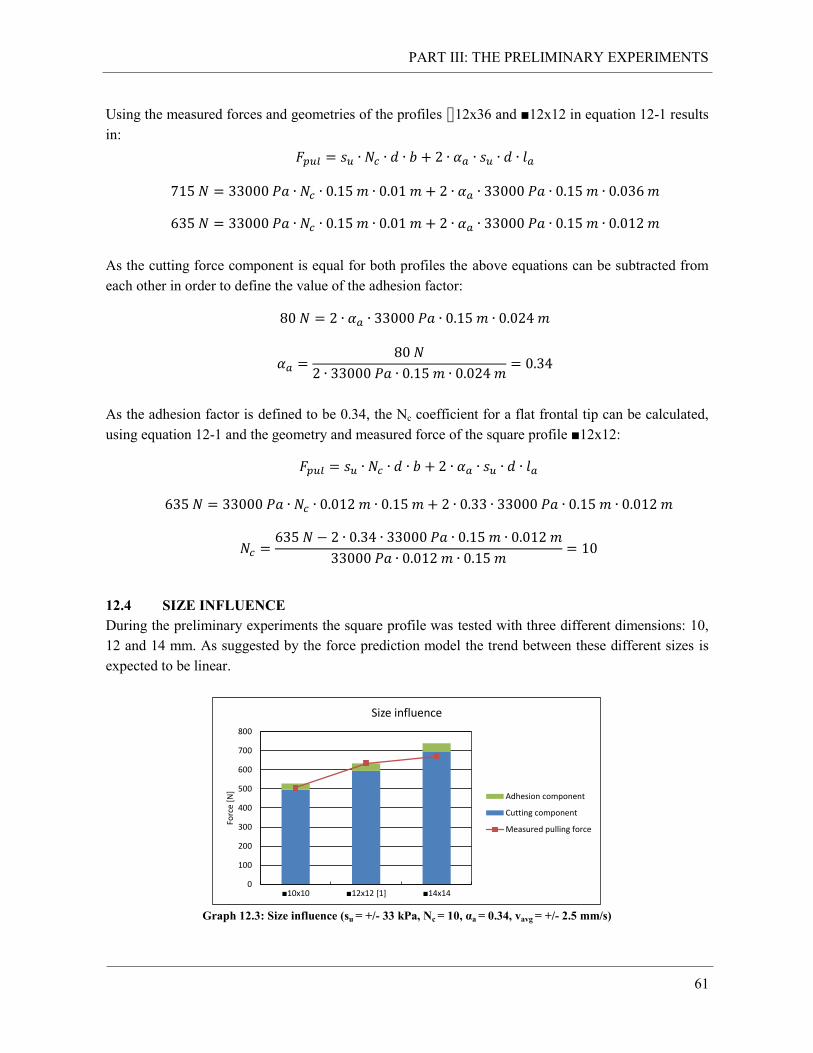
PART III: THE PRELIMINARY EXPERIMENTS
61
Using the measured forces and geometries of the profiles ⌷12x36 and ■12x12 in equation 12-1 results
in:
As the cutting force component is equal for both profiles the above equations can be subtracted from
each other in order to define the value of the adhesion factor:
As the adhesion factor is defined to be 0.34, the Nc coefficient for a flat frontal tip can be calculated,
using equation 12-1 and the geometry and measured force of the square profile ■12x12:
12.4 SIZE INFLUENCE
During the preliminary experiments the square profile was tested with three different dimensions: 10,
12 and 14 mm. As suggested by the force prediction model the trend between these different sizes is
expected to be linear.
Graph 12.3: Size influence (su = +/- 33 kPa, Nc = 10, αa = 0.34, vavg = +/- 2.5 mm/s)
0
100
200
300
400
500
600
700
800
■10x10 ■12x12 [1] ■14x14
Forc
e [N
]
Size influence
Adhesion component
Cutting component
Measured pulling force
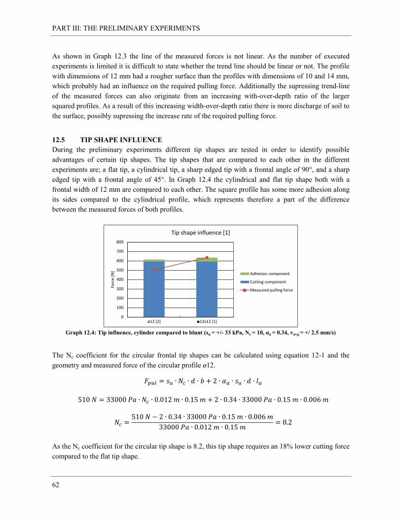
PART III: THE PRELIMINARY EXPERIMENTS
62
As shown in Graph 12.3 the line of the measured forces is not linear. As the number of executed
experiments is limited it is difficult to state whether the trend line should be linear or not. The profile
with dimensions of 12 mm had a rougher surface than the profiles with dimensions of 10 and 14 mm,
which probably had an influence on the required pulling force. Additionally the supressing trend-line
of the measured forces can also originate from an increasing with-over-depth ratio of the larger
squared profiles. As a result of this increasing width-over-depth ratio there is more discharge of soil to
the surface, possibly supressing the increase rate of the required pulling force.
12.5 TIP SHAPE INFLUENCE
During the preliminary experiments different tip shapes are tested in order to identify possible
advantages of certain tip shapes. The tip shapes that are compared to each other in the different
experiments are; a flat tip, a cylindrical tip, a sharp edged tip with a frontal angle of 90°, and a sharp
edged tip with a frontal angle of 45°. In Graph 12.4 the cylindrical and flat tip shape both with a
frontal width of 12 mm are compared to each other. The square profile has some more adhesion along
its sides compared to the cylindrical profile, which represents therefore a part of the difference
between the measured forces of both profiles.
Graph 12.4: Tip influence, cylinder compared to blunt (su = +/- 33 kPa, Nc = 10, αa = 0.34, vavg = +/ 2.5 mm/s)
The Nc coefficient for the circular frontal tip shapes can be calculated using equation 12-1 and the
geometry and measured force of the circular profile ø12.
As the Nc coefficient for the circular tip shape is 8.2, this tip shape requires an 18% lower cutting force
compared to the flat tip shape.
0
100
200
300
400
500
600
700
800
ø12 [2] ■12x12 [1]
Forc
e [N
]
Tip shape influence [1]
Adhesion component
Cutting component
Measured pulling force

PART III: THE PRELIMINARY EXPERIMENTS
63
The profile ⌷12x36 with flat frontal tip shape is modified to a profile with a sharp tip of 90° and a
profile with a sharp tip of 45°. The measured forces for the profile 12x36 with different tip shapes are
plotted in Graph 12.5.
Graph 12.5: Tip influence, 90° and 45° sharp edged tip compared to blunt
(su = +/- 33 kPa, Nc = 10, αa = 0.34, vavg = +/- 2.5 mm/s)
As can be seen from Graph 12.4 the measured force of the 90° sharp edged tip is only a bit smaller
than the measured force of the profile with a flat frontal tip. This means that the cutting forces of both
tip shapes are equal to each other and the 90° sharp edged tip thus also has an Nc coefficient of 10. The
influence of the 90° tip shape is probably limited due to the shape of the failure zones. As shown in
Figure 5.1 a wedge of soil is formed in the active Rankine zone in front of the flat frontal tip shape,
which will move along with the profile. In clay soils this soil wedge has a sharp frontal angle of 90°,
which is equal to the 90° tip shape, making the influence of this shape limited.
As can be seen from Graph 12.5 the measured force of the 45° sharp edged tip shape is significantly
lower than the measured forces of the blunt and 90° sharp edged tip shapes. The Nc coefficient for the
sharp edged 90° tip can be calculated using equation 12-1 and the geometry and measured force of the
sharp edged profile 12x36 <=45°:
As the Nc coefficient for the 45° sharp edged tip shape is 8.2, this tip shape requires an 18% lower
cutting force compared to the flat tip shape.
The values of the Nc coefficients as calculated in this section are based on a width-over-depth ratio of
1:6. For other width-over-depth ratios the Nc coefficients are probably different, but it is
acknowledged that the tip shape has an influence on the required cutting force. The Nc coefficients for
0
100
200
300
400
500
600
700
800
⌷12x36 12x36 <=90° 12x36 <=45°
Forc
e [N
]
Tip shape influence [2]
Adhesion component
Cutting component
Measured pulling force
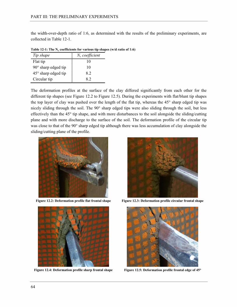
PART III: THE PRELIMINARY EXPERIMENTS
64
the width-over-depth ratio of 1:6, as determined with the results of the preliminary experiments, are
collected in Table 12-1.
Table 12-1: The Nc coefficients for various tip shapes (w/d ratio of 1:6)
Tip shape Nc coefficient
Flat tip 10
90° sharp edged tip 10
45° sharp edged tip 8.2
Circular tip 8.2
The deformation profiles at the surface of the clay differed significantly from each other for the
different tip shapes (see Figure 12.2 to Figure 12.5). During the experiments with flat/blunt tip shapes
the top layer of clay was pushed over the length of the flat tip, whereas the 45° sharp edged tip was
nicely sliding through the soil. The 90° sharp edged tips were also sliding through the soil, but less
effectively than the 45° tip shape, and with more disturbances to the soil alongside the sliding/cutting
plane and with more discharge to the surface of the soil. The deformation profile of the circular tip
was close to that of the 90° sharp edged tip although there was less accumulation of clay alongside the
sliding/cutting plane of the profile.
Figure 12.2: Deformation profile flat frontal shape
Figure 12.3: Deformation profile circular frontal shape
Figure 12.4: Deformation profile sharp frontal shape
Figure 12.5: Deformation profile frontal edge of 45°
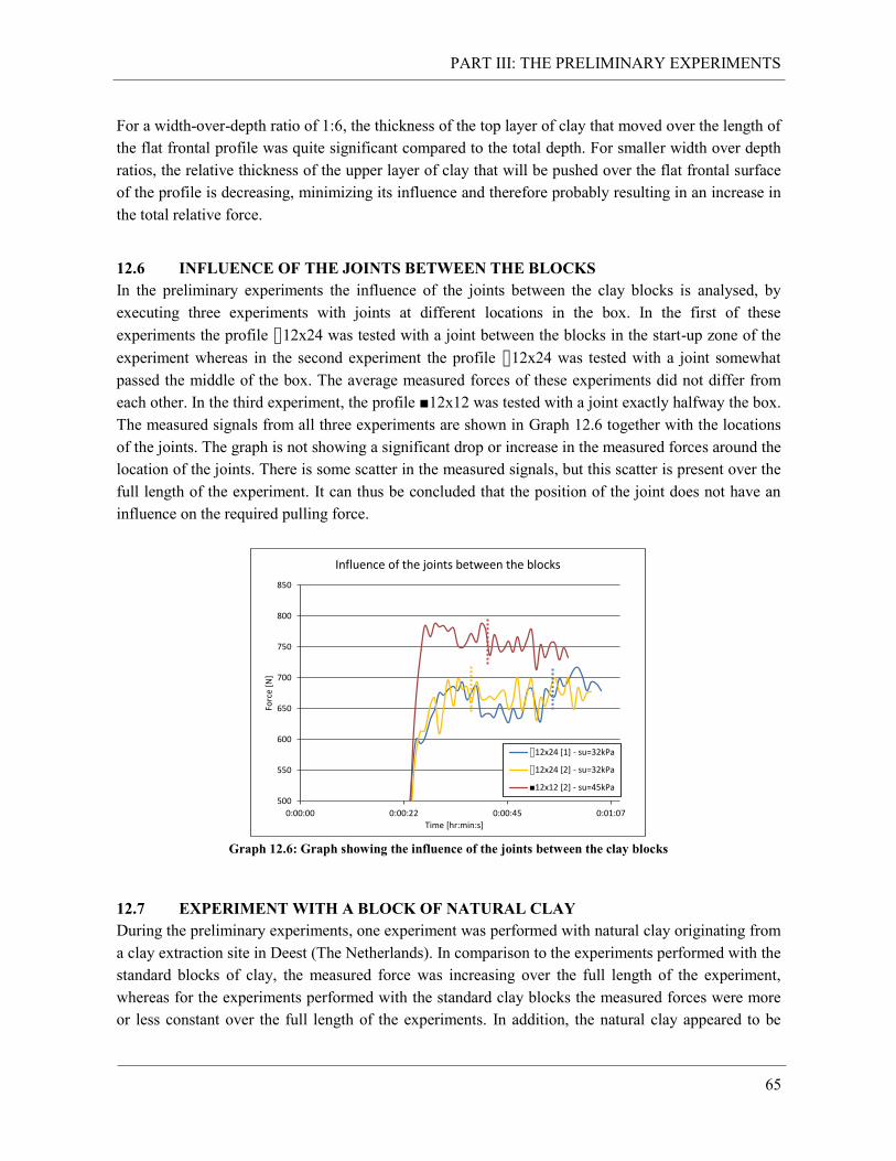
PART III: THE PRELIMINARY EXPERIMENTS
65
For a width-over-depth ratio of 1:6, the thickness of the top layer of clay that moved over the length of
the flat frontal profile was quite significant compared to the total depth. For smaller width over depth
ratios, the relative thickness of the upper layer of clay that will be pushed over the flat frontal surface
of the profile is decreasing, minimizing its influence and therefore probably resulting in an increase in
the total relative force.
12.6 INFLUENCE OF THE JOINTS BETWEEN THE BLOCKS
In the preliminary experiments the influence of the joints between the clay blocks is analysed, by
executing three experiments with joints at different locations in the box. In the first of these
experiments the profile ⌷12x24 was tested with a joint between the blocks in the start-up zone of the
experiment whereas in the second experiment the profile ⌷12x24 was tested with a joint somewhat
passed the middle of the box. The average measured forces of these experiments did not differ from
each other. In the third experiment, the profile ■12x12 was tested with a joint exactly halfway the box.
The measured signals from all three experiments are shown in Graph 12.6 together with the locations
of the joints. The graph is not showing a significant drop or increase in the measured forces around the
location of the joints. There is some scatter in the measured signals, but this scatter is present over the
full length of the experiment. It can thus be concluded that the position of the joint does not have an
influence on the required pulling force.
Graph 12.6: Graph showing the influence of the joints between the clay blocks
12.7 EXPERIMENT WITH A BLOCK OF NATURAL CLAY
During the preliminary experiments, one experiment was performed with natural clay originating from
a clay extraction site in Deest (The Netherlands). In comparison to the experiments performed with the
standard blocks of clay, the measured force was increasing over the full length of the experiment,
whereas for the experiments performed with the standard clay blocks the measured forces were more
or less constant over the full length of the experiments. In addition, the natural clay appeared to be
500
550
600
650
700
750
800
850
0:00:00 0:00:22 0:00:45 0:01:07
Forc
e [N
]
Time [hr:min:s]
Influence of the joints between the blocks
⌷12x24 [1] - su=32kPa
⌷12x24 [2] - su=32kPa
■12x12 [2] - su=45kPa
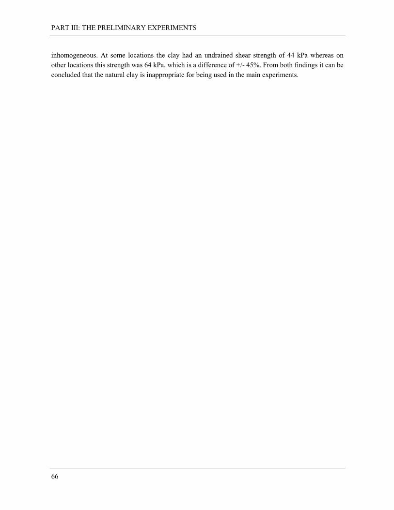
PART III: THE PRELIMINARY EXPERIMENTS
66
inhomogeneous. At some locations the clay had an undrained shear strength of 44 kPa whereas on
other locations this strength was 64 kPa, which is a difference of +/- 45%. From both findings it can be
concluded that the natural clay is inappropriate for being used in the main experiments.
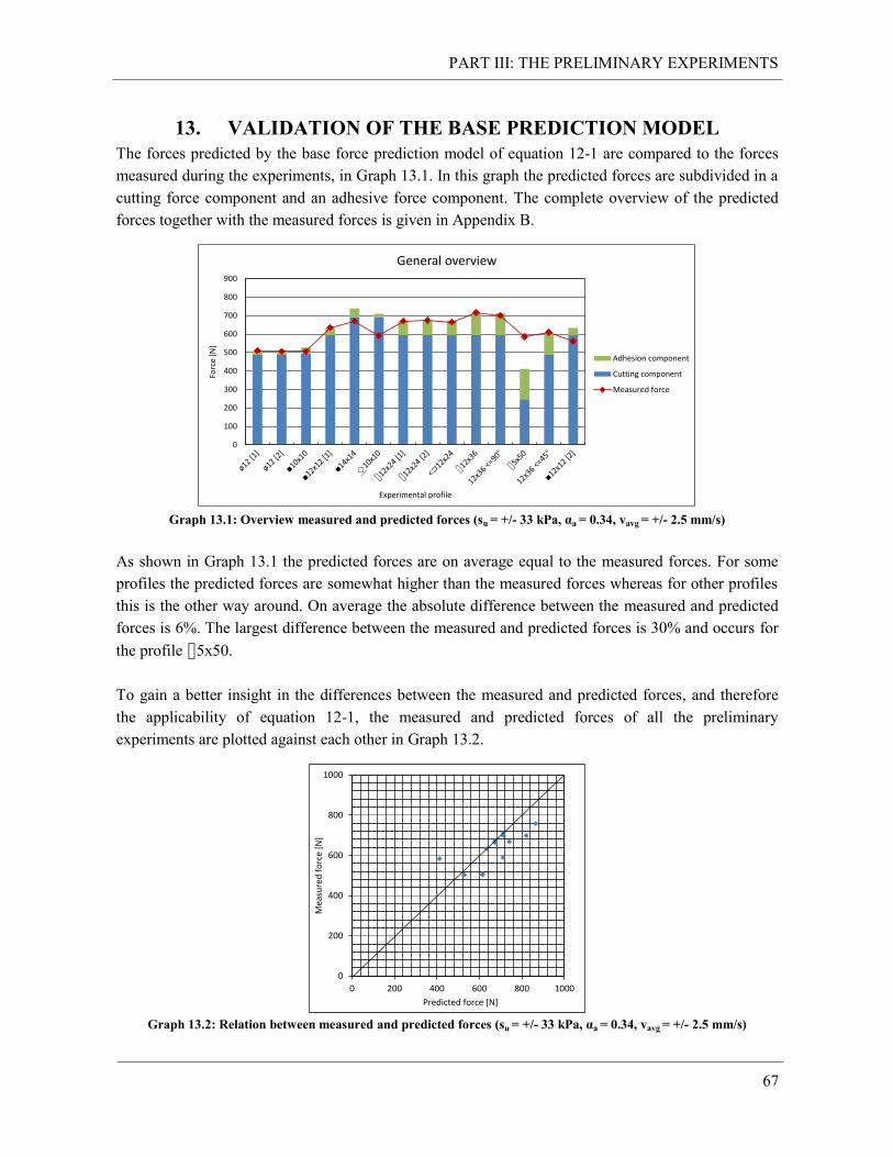
PART III: THE PRELIMINARY EXPERIMENTS
67
13. VALIDATION OF THE BASE PREDICTION MODEL
The forces predicted by the base force prediction model of equation 12-1 are compared to the forces
measured during the experiments, in Graph 13.1. In this graph the predicted forces are subdivided in a
cutting force component and an adhesive force component. The complete overview of the predicted
forces together with the measured forces is given in Appendix B.
Graph 13.1: Overview measured and predicted forces (su = +/- 33 kPa, αa = 0.34, vavg = +/- 2.5 mm/s)
As shown in Graph 13.1 the predicted forces are on average equal to the measured forces. For some
profiles the predicted forces are somewhat higher than the measured forces whereas for other profiles
this is the other way around. On average the absolute difference between the measured and predicted
forces is 6%. The largest difference between the measured and predicted forces is 30% and occurs for
the profile ⌷5x50.
To gain a better insight in the differences between the measured and predicted forces, and therefore
the applicability of equation 12-1, the measured and predicted forces of all the preliminary
experiments are plotted against each other in Graph 13.2.
Graph 13.2: Relation between measured and predicted forces (su = +/- 33 kPa, αa = 0.34, vavg = +/- 2.5 mm/s)
0
100
200
300
400
500
600
700
800
900
Forc
e [N
]
Experimental profile
General overview
Adhesion component
Cutting component
Measured force
0
200
400
600
800
1000
0 200 400 600 800 1000
Mea
sure
d f
orc
e [N
]
Predicted force [N]

PART III: THE PRELIMINARY EXPERIMENTS
68
From this graph it can be conclude that the base prediction model is a reasonable model to estimate the
required pulling forces for very short profiles moving parallel to the surface.
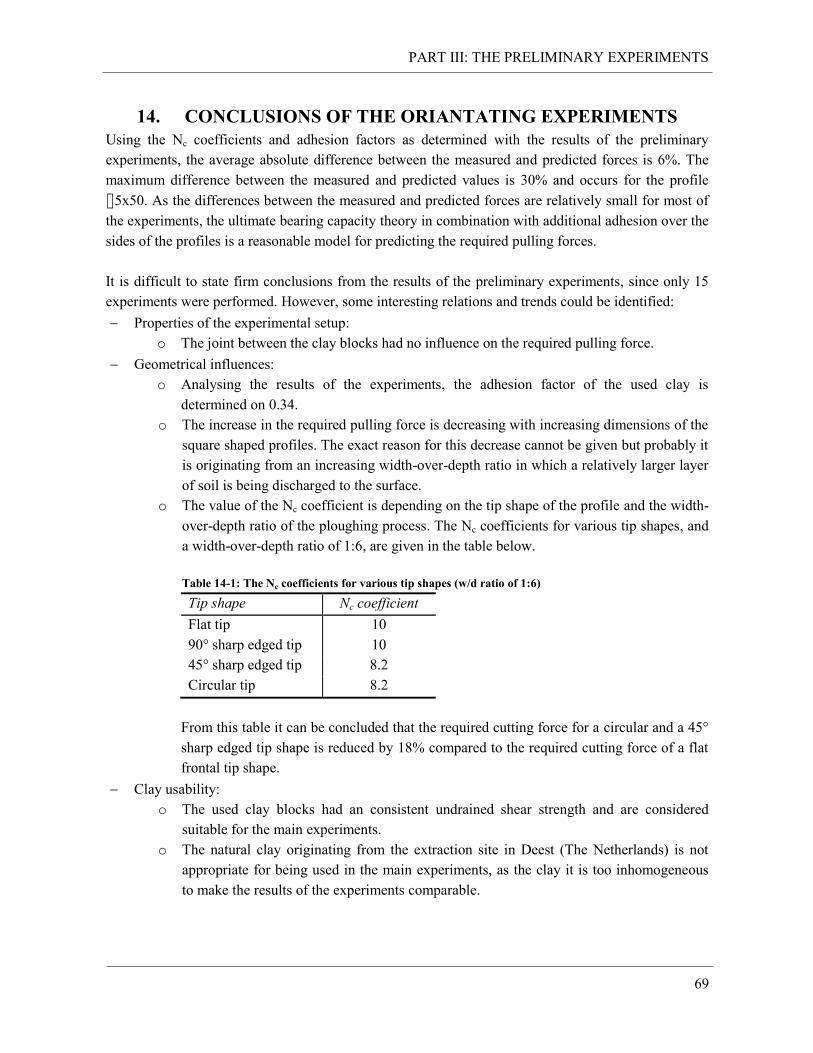
PART III: THE PRELIMINARY EXPERIMENTS
69
14. CONCLUSIONS OF THE ORIANTATING EXPERIMENTS
Using the Nc coefficients and adhesion factors as determined with the results of the preliminary
experiments, the average absolute difference between the measured and predicted forces is 6%. The
maximum difference between the measured and predicted values is 30% and occurs for the profile
⌷5x50. As the differences between the measured and predicted forces are relatively small for most of
the experiments, the ultimate bearing capacity theory in combination with additional adhesion over the
sides of the profiles is a reasonable model for predicting the required pulling forces.
It is difficult to state firm conclusions from the results of the preliminary experiments, since only 15
experiments were performed. However, some interesting relations and trends could be identified:
Properties of the experimental setup:
o The joint between the clay blocks had no influence on the required pulling force.
Geometrical influences:
o Analysing the results of the experiments, the adhesion factor of the used clay is
determined on 0.34.
o The increase in the required pulling force is decreasing with increasing dimensions of the
square shaped profiles. The exact reason for this decrease cannot be given but probably it
is originating from an increasing width-over-depth ratio in which a relatively larger layer
of soil is being discharged to the surface.
o The value of the Nc coefficient is depending on the tip shape of the profile and the width-
over-depth ratio of the ploughing process. The Nc coefficients for various tip shapes, and
a width-over-depth ratio of 1:6, are given in the table below.
Table 14-1: The Nc coefficients for various tip shapes (w/d ratio of 1:6)
Tip shape Nc coefficient
Flat tip 10
90° sharp edged tip 10
45° sharp edged tip 8.2
Circular tip 8.2
From this table it can be concluded that the required cutting force for a circular and a 45°
sharp edged tip shape is reduced by 18% compared to the required cutting force of a flat
frontal tip shape.
Clay usability:
o The used clay blocks had an consistent undrained shear strength and are considered
suitable for the main experiments.
o The natural clay originating from the extraction site in Deest (The Netherlands) is not
appropriate for being used in the main experiments, as the clay it is too inhomogeneous
to make the results of the experiments comparable.

PART III: THE PRELIMINARY EXPERIMENTS
70
71
BIBLIOGRAPHY
Allan, P. (1998) Selecting Appropriate Cable Burial Depths, A methodology in selecting appropriate
cable burial depths. IBC Conference on Submarine Communications. The future of network
infrastructure, Cannes, November 1998.
Aubeny C.P. & Shi H. (2007) Effect of rate-dependent soil strength on cylinders penetrating into soft
clay. IEEE journal of oceanic engineering, Vol. 32, No. 1, Page 49-56.
Barnes, G. (2010) Soil Mechanics, Principles and practice. Palgrave Macmillan.
Brinch Hansen J. (1961) A general formula for bearing capacity, The Danish geotechnical institute,
Bulletin No 11, Page 37-46.
Beindorff, R. (2011). New ways to calculate forces and velocities on a submarine narrow trench
lough, in sandy soil. Thesis report Delft University of Technology.
Dayal, U. & Allen, J.H. (1975) The Effect of Penetration Rate on the Strength of Remolded Clay and
Sand Samples, Canadian Geotechnical Journal 12, Page 336-348.
Gilbert Gedeon, P.E. (1992) Bearing Capacity of Soils. U.S. Army Corps of Engineers, Engineer
manual No. 1110-1905.
Godwin, R.J. & Spoor, G. (1977) Soil failure with narrow tines. J. agric. Engng Res., Page 213-228.
Grisso R.D. & Perumpral J.V. (1985) Review of models for predicting performance of narrow tillage
tools. TRANSACTIONS of the ASAE, Vol. 28, Page 1062-1067
Hettiaratchi, D.R.P. & Reece A.R. (1966) The calculation of passive pressure in two-dimensional soil
failure. J. agric. Engng Res. 11, Page 89-107.
Hettiaratchi, D.R.P. & Reece, A.R. (1967) Symmetrical three-dimensional soil failure. Journal of
Terramechanics, Vol 4, No. 3, Page 45-67.
Hettiaratchi, D.R.P. & Reece A.R. (1974) The calculation of passive soil resistance. Géotechnique 24,
No. 3, Page 289-310.
Kroes, G. (2010) Subsea cable installation, a technical guide. Magazine for The offshore wind
industry No 04.
72
Kulhawy, F. & Mayne, P. (1990) Manual on estimating soil properties for foundation design.
Research project by the geotechnical engineering group of the Cornell university.
McKyes, E. & Ali, O.S. (1977) The cutting of soil by narrow blades. Journal of Terramechanics, Vol.
14, No. 3, Page 43-58.
McKyes, E. (1985) Soil cutting and tillage. Elsevier Science Publisher B.V.
Meyerhof G.G. (1951) The ultimate bearing capacity of foundations, Géotechnique Vol 2, Issue 4.
Miedema, S.A. (1992) New Developments of Cutting Theories with respect to Dredging, the Cutting of
Clay. Proc. WODCON XIII, Bombay India 1992.
Miedema S.A. (2012) Dredging processes, The cutting of sand, clay & rock, Soil mechanics. Lecture
notes Delft University of Technology.
Mole, P., Featherstone, J., & Winter, S. (1997) Cable protection - Solutions through new installation
and burial approaches. Cable & Wireless Marine.
Nobel A. (2013) On the excavation process of a moving vertical jet in cohesive soil. Doctoral thesis
Delft University of Technology.
Perumpral J.V., Grisso R.D. & Desai C.S. (1983) A soil-toll model based on limit equilibrium
analysis. Transactions of the ASAE 26(4), Page 991-995.
Reece, A.R. & Grinsted, T.W. (1986) Soil mechanics of submarine ploughs. OTC 5341.
Sharifat K. (1999) Soil translocation with tillage tools. Phd report at the Department of Agricultural
and Bioresource Engineering at the University of Saskatchewan.
Terzaghi, K. (1943) Theoretical Soil Mechanics. John Wiley and Sons, New York (1943)
Tomlinson (1970) The adhesion of piles driven in stiff clay. CIRIA Research report No. 26.
Verruijt, A. (2007) Soil Mechanics. VSSD.
Wismer R.D. & Luth H.J. (1972) Rate effects in soil cutting. Journal of Terramechanics, Vol 8, No. 3,
Page 11-21.
Zelenin, A. N. (1950) Basic physics of the theory of soil cutting. Moscow, Russia: Kolos