1 | P a g e

Conditional Facies Modeling Using an Improved Progressive

Growing of Generative Adversarial Networks (GANs)

Suihong Song1,2,3, Tapan Mukerji3, Jiagen Hou1,2,*

1 State Key Laboratory of Petroleum Resources and Prospecting, China University of Petroleum (Beijing),

Beijing, 102249, China. Email: songsuihong@126.com

2 College of Geoscience, China University of Petroleum (Beijing), Beijing, 102249, China.

3 Stanford University, 367 Panama St, Stanford, CA 94305, USA.

This is a non-peer reviewed preprint submitted to EarthArXiv.

Abstract:

Conditional facies modeling combines geological spatial patterns with different types of

observed data, to build earth models for predictions of subsurface resources. Recently,

researchers have used generative adversarial networks (GANs) for conditional facies modeling,

where an unconditional GAN is first trained to learn the geological patterns using the original

GANs loss function, then appropriate latent vectors are searched to generate facies models that

are consistent with the observed conditioning data. A problem with this approach is that the time-

consuming search process needs to be conducted for every new conditioning data. As an

alternative, we improve GANs for conditional facies modeling by introducing an extra

condition-based loss function and adjusting the architecture of the generator to take the

conditioning data as inputs, based on progressive growing of GANs. The condition-based loss

function is defined as the inconsistency between the input conditioning value and the

corresponding characteristics exhibited by the output facies model, and forces the generator to

learn the ability of being consistent with the input conditioning data, together with the learning

of geological patterns. Our input conditioning factors include global features (e.g. the mud facies

proportion) alone, local features such as sparse well facies data alone, and joint combination of

global features and well facies data. After training, we evaluate both the quality of generated

facies models and the conditioning ability of the generators, by manual inspection and

quantitative assessment. The trained generators are quite robust in generating high-quality facies

models conditioned to various types of input conditioning information.

Keywords:

Conditional facies modeling, Generative Adversarial Networks, GANs, Progressive Growing of

2 | P a g e

GANs, Deep learning, Geological pattern, Reservoir forecast

Key points:

(1) Progressive growing of Generative Adversarial Networks (GANs) is improved for facies

modeling conditioned to various types of data

(2) Trained generators can directly be used for practical facies modeling without additional

searching of appropriate latent vectors

(3) Trained generators are robust in generating realistic facies models conditioned to global

features, well data, or their joint combination

1. Introduction

Geological facies modeling is fundamental to the accurate prediction of subsurface

resources, such as groundwater, petroleum, and carbon storage potential. Many geostatistical

facies modeling approaches have been developed in the past decades, such as variogram-based

methods, multiple points statistics (MPS)-based methods, object-based methods, and process-

mimicking methods (Pyrcz and Deutsch 2014). These approaches have various advantages and

disadvantages, and they have been widely used in different scenarios. Some of them are still

under research, such as the recent development of the tree-based direct sampling MPS method

(Zuo et al. 2020).

Basically, geological facies modeling is a process of generating 2D/3D spatial facies

models with realistic geological spatial patterns, given various types of observed data. From the

perspective of deep learning, geological facies modeling belongs to the class of generative

problems, in which a generative model is trained to reproduce a probability distribution given

many samples from that distribution (Ian Goodfellow, Yoshua Bengio 2015). Some widely used

deep generative models include deep sigmoid belief networks (Gan et al. 2015), pixel recurrent

neural network (RNN) and pixel convolutional neural networks (CNN) (Van Den Oord et al.

2016b), variational autoencoders (VAE) (Larochelle and Murray 2011; Rezende et al. 2014), and

especially generative adversarial networks (GANs) (Goodfellow et al. 2014).

Among these generative models, GANs generates very realistic results and have been

most widely studied and applied. In the GANs framework, there is a generator network and a

discriminator network. The goal of the generator is to “cheat” the discriminator by generating

realistic results, while the goal of the discriminator is to avoid being cheated by the generator by

discriminating the real data from the outputs of the generator. Finally, after iterations of training,

the generator is kept for further generative applications. Appendix A.1 and A.2 give more details

3 | P a g e

about GANs. Many variants of GANs have been developed, such as conditional GANs (Mirza

and Osindero 2014), cycle GANs (Zhu et al. 2017), and bidirectional GANs (Dumoulin et al.

2016). Karras et al. (2017) proposed progressive growing of GANs, where the networks in the

GANs are trained layer by layer. This progressive GAN training method allows the features to be

learned from large scales to fine scales, and proves to perform much better than the conventional

GAN training method in terms of the training speed, stability, and the quality of the generated

results. Appendix B shows how progressive growing of GANs is applied for an unconditional

facies modeling case. Based on the progressive growing of GANs, Karras et al. (2018) further

proposed style GANs. GANs has been successfully used in many areas, including image

generation (Karras et al., 2017), image inpainting (Van Den Oord et al. 2016a), super-resolution

image creation (Ledig et al. 2016), text-to-image translation (Reed et al. 2016), and object

segmentation (Isola et al. 2016).

Many researchers have studied the application of GANs for geological facies modeling.

Mosser et al. (2017) and Mosser et al. (2018) used deep convolutional GANs for reconstruction

of 3D solid-void structure of porous media and micro-CT-scale oolitic Ketton limestone. Chan &

Elsheikh (2017) used convolutional GANs combined with the Wasserstein loss to generate

geological facies models. These works are focused on unconditional realizations.

In most cases, geological facies models need to be conditioned to observed data (e.g.,

facies observed in wells). To achieve conditioning to observed data, some researchers have used

“post-GANs” approaches, where unconditional GANs are first trained, and then appropriate

latent vectors that generate models consistent with the observed data are searched. Nesvold &

Mukerji (2019), Mosser et al. (2020), and Laloy et al. (2018) used Markov Chain Monte Carlo

(MCMC) algorithms to search for the appropriate latent vectors. Dupont et al. (2018) and Zhang

et al. (2019) applied gradient descent method to obtain the appropriate latent vectors. With the

above MCMC or the gradient decent optimization algorithm, only one appropriate latent vector

is searched every time. In situations where many conditional facies realizations are required,

e.g., uncertainty quantification, the latent vector searching process needs to be conducted many

times, which is, however, slow and inconvenient. Therefore, Chan & Elsheikh (2019) proposed

to train an extra inference neural network to map a known distribution, e.g., Gaussian, into the

distribution of the appropriate latent vectors, so that multiple samples from the known

distribution can be directly mapped into multiple appropriate latent vectors by the inference

network. One problem for the “post-GANs” approaches is that, once the values of the observed

data change, the time-consuming “post-GANs” process of finding the appropriate latent vector

(i.e., MCMC, gradient descent, or inference network training) needs to be performed again.

Sun (2018) applied cycle GANs for bidirectional domain transformation between high-

dimensional parameter space and the corresponding model state space. The output of the GAN is

4 | P a g e

directly conditioned to the GAN’s input. Similarly, Mosser et al. (2018) also used cycle GANs

for domain transformation between seismic velocity and the geological model. Theoretically,

cycle GANs stands out in unsupervised domain transformation tasks, where paired training

dataset between two domains are difficult to obtain. One problem for cycle GANs is that

concurrently training two GANs is quite difficult and unstable.

In addition, Zhong et al. (2019) used conditional GANs and “U-Net” design to transfer the

permeability distribution map into CO2 saturation maps at different time steps. The GAN takes

the time step data and the permeability map as two channels in the input and generates CO2

saturation maps as outputs. The output maps are conditioned to the input permeability and the

time steps. Such a GAN architecture may also be extended for the conditional facies modeling

task. Compared to the “post-GANs” processes, this architecture is more straightforward for

achieving multiple conditionings; however, the “U-Net” design in this architecture increases the

number of trainable parameters, leading to increased training difficulties.

Therefore, in this paper, we improve GANs for conditional facies modeling, by

introducing an extra condition-based loss function and adjusting the architecture of the generator

to take conditioning data as inputs, in the context of the progressive growing of GANs. The

conditioning information for the facies modeling include prior global features (e.g., the facies

proportions, and the sinuosity of channels) alone, sparse well facies data (“hard data”) alone, and

the joint combination of global features and well facies data. After training, the generator can be

directly used for practical conditional facies modeling without further training or “post-GANs”

processes.

This paper is organized as follows. Section 2 shows how the GAN framework is modified

for facies modeling conditioned to global features, well facies data, and their combination.

Section 3 illustrates how the trained generators are evaluated in terms of the quality of the

generated facies models and the conditioning ability of the trained generators to various types of

input conditioning data. Section 4 shows how necessary dataset are built for the training and

testing of our GANs. Section 5 presents the results, evaluation, and analyses of the trained

generators. Finally, conclusions are provided in section 6.

2. GANs Improvement

For conditional facies modeling the generator needs two types of abilities: one is to be

consistent with the geological patterns, and the other is to be consistent with the conditioning

data. In GAN-based unconditional facies modeling, the generator learns the knowledge about

geological patterns, and this allows the generator to simulate realistic facies models in an

unconditional manner. To enforce the generator to be consistent with the given conditioning data

5 | P a g e

(or conditioning ability) at the same time, we propose a workflow (Fig. 1) as follows. First, we

design the architecture of the generator (𝐺𝜃) to also take the given conditioning information

(𝑐𝑜𝑛0) as an input together with the latent vector (z). Second, we construct a function (𝑓𝑐𝑜𝑛(𝐹)),

which maps the facies model (𝐹) into the given conditioning domain (𝑐𝑜𝑛). Third, we use

𝑓𝑐𝑜𝑛(𝐹) to map the output facies model of the generator back into the conditioning domain, i.e.,

𝑐𝑜𝑛1 = 𝑓𝑐𝑜𝑛[𝐺𝜃(𝑧, 𝑐𝑜𝑛0)] , where in general 𝑐𝑜𝑛1 may not be equal to 𝑐𝑜𝑛0 ; we define a

condition-based loss function as some form of the distance between 𝑐𝑜𝑛1 and 𝑐𝑜𝑛0 (Equation

(1)):

𝐿(𝐺𝜃)𝑐𝑜𝑛 = 𝐷𝑖𝑠𝑡(𝑐𝑜𝑛1, 𝑐𝑜𝑛0) = 𝔼𝑧~𝑝𝑧,𝑐𝑜𝑛0~𝑝𝑐𝑜𝑛0𝐷𝑖𝑠𝑡(𝑓𝑐𝑜𝑛[𝐺𝜃(𝑧, 𝑐𝑜𝑛0)], 𝑐𝑜𝑛0) (1)

Here, 𝐿(𝐺𝜃)𝑐𝑜𝑛 is the condition-based loss function, and 𝐷𝑖𝑠𝑡(𝑐𝑜𝑛1, 𝑐𝑜𝑛0) is some type of

distance (made more specific later) between 𝑐𝑜𝑛1 and 𝑐𝑜𝑛0, while 𝑝𝑧 is the distribution of 𝑧, and

𝑝𝑐𝑜𝑛0 is the distribution of 𝑐𝑜𝑛0. The condition-based loss function is combined with the original

GAN loss function as shown in Equation (2):

𝐿(𝐺𝜃 , 𝐷𝜑)𝑐𝑜𝑚𝑏𝑖𝑛𝑒𝑑

= 𝐿(𝐺𝜃 , 𝐷𝜑) + 𝛽𝐿(𝐺𝜃)𝑐𝑜𝑛 (2)

where, 𝐿(𝐺𝜃, 𝐷𝜑)𝑐𝑜𝑚𝑏𝑖𝑛𝑒𝑑

is the combined loss, 𝐿(𝐺𝜃 , 𝐷𝜑) is the original GAN loss function,

𝐷𝜑 is the discriminator, and 𝛽 is the weight for 𝐿(𝐺𝜃)𝑐𝑜𝑛.

Finally, we apply this combined loss to train the GAN in a progressive growing manner.

The condition-based loss function only affects the training of the generator. This workflow is

universal for all forms of conditioning, so it is called the general workflow hereafter in this

paper.

In this general workflow, there are two “objectives” working: (1) GAN framework and the

original GAN loss function pushes the generator to map its input into the distribution of the

training dataset (𝑝𝑑𝑎𝑡𝑎), so the output facies model of the generator would be realistic, i.e.,

𝐺𝜃(𝑧, 𝑐𝑜𝑛0) → 𝑝𝑑𝑎𝑡𝑎 (shown by purple arrows in Fig. 1); (2) the condition-based loss function

pushes the generator to the proper subspace of the distribution that is consistent with the input

conditioning value through 𝑓𝑐𝑜𝑛(𝐹), i.e., 𝑓𝑐𝑜𝑛[𝐺𝜃(𝑧, 𝑐𝑜𝑛0)] → 𝑐𝑜𝑛0 (shown by green arrows in

Fig. 1). With the above two objectives, the output facies model of the generator is both realistic

in terms of spatial patterns, and consistent with the input conditioning data.

6 | P a g e

Fig. 1. A schematic for the conditional facies modeling workflow (the general workflow). Axis

𝑐𝑜𝑛 and 𝑧 represents the condition and the latent vector, respectively. The size of the light blue

cross represents certain characteristics (e.g., the width of channel) exhibited by the generated

facies model, and these characteristics correspond to the input conditioning value.

Three most important elements in the general workflow are 1) the architecture of

generator to take the conditioning data as input, 2) the construction of 𝑓𝑐𝑜𝑛(𝐹), and 3) the

definition of the distance between 𝑐𝑜𝑛1 and 𝑐𝑜𝑛0 in the condition-based loss function. These

elements are decided depending on the input conditioning data type. In the following parts, we

discuss these three elements in detail, with conditioning data as non-spatial global features,

spatially sparse well facies data, and both jointly.

The GAN architecture for conditional facies modeling in this paper is based on an

unconditional GAN for facies modeling which is described in detail in Appendix B. The

generator and the discriminator in the unconditional GAN are called the base generator and the

base discriminator in this paper. For conditioning, the generators are modified from the base

generator; the discriminator is modified from the base discriminator for the case of conditioning

to global features alone and the case of conditioning to both global features and well facies data,

and remains the same as the base discriminator for the case of conditioning to well facies data

alone. The resolution of the base generator’s output is 64×64 (2D). The Wasserstein loss

function with gradient penalty (W-gp) (Equation (A4) in Appendix A) and other settings of

training in the unconditional work (Appendix B.2) are also used in this work. After training, the

generator is kept for further evaluation and practical applications.

2.1 Facies modeling conditioned to global features

In practice, sometimes we need to simulate facies models that have certain types of

features, such as the proportion of facies and the sinuosity of channels. These features describe

7 | P a g e

the global characteristics of the facies models and are not related to the spatial distribution of

facies, so these features are called global features (𝑔) in this paper.

According to the general workflow, we specify the three elements for the facies modeling

conditioned to global features as follows. First, we modify the input layer of the base generator

to also include the global features, and accordingly adjust the first fully connected layer of the

base generator (Fig. 2). Second, the facies model-to-condition function (specifically called the

facies model-to-global features function in this case, 𝑓𝑔(𝐹)) can be easily obtained for a small

number of global features, such as facies proportion, but can be difficult to calculate for other

global features, such as the sinuosity, orientation, width, wavelength, and amplitude of channel

complexes, as it could involve some image processing on every generated facies model. For

example, Clerici & Perego (2016) proposed to first obtain the centerline of a channel by

gradually moving two channel boundary curves towards each other, then calculate the width of

the channel by averaging many transect lines that are orthogonal to the centerline, and finally

calculate the sinuosity index by dividing the length of the centerline by the distance between the

start and end points of the centerline. However, such calculations are difficult to be expressed

using parameterized functions, and would be specific to each global feature. An efficient and

more general way to obtain 𝑓𝑔(𝐹) (valid for any global feature) is to train a separate deep neural

network with labeled training dataset, where the input is the facies model and the outputs are the

global features. Considering that the architecture and function of such a deep neural network are

very similar to that of the discriminator, we propose to integrate 𝑓𝑔(𝐹) into the discriminator so

that the discriminator produces a score value (s) and an array of the global feature values (Fig.

2). Third, the distance between the input and output global features in the condition-based loss

function (Equation (1)) is defined as the L2 norm distance.

Fig. 2. (a) Two-step procedure of the facies modeling conditioned to global features. First, we train

𝑓𝑔(𝐹) with training facies models and corresponding global features. Second, based on the trained

𝑓𝑔(𝐹), we train the modified GANs. (b) The discriminator is modified from the base discriminator

to integrate the 𝑓𝑔(𝐹) network, and it produces a score value (s) and the global feature values. In

this way, we only need to train the modified GAN.

8 | P a g e

As the Wasserstein loss function with gradient penalty (W-gp) is used, we combine

Equations (A4), (1), and (2) to derive the final loss function of the modified generator in this

case as follows:

𝐿(𝐺𝜃)𝑐𝑜𝑚𝑏𝑖𝑛𝑒𝑑 = 𝔼𝑧~𝑝𝑧,𝑔~𝑝𝑔{−𝐷𝑠𝜑

(𝐺𝜃(𝑧, 𝑔)) + 𝛽 ∥ 𝐷𝑔𝜑[𝐺𝜃(𝑧, 𝑔)] − 𝑔 ∥2} (3)

where, 𝑝𝑧 and 𝑝𝑔 are the distributions of the latent vector (𝑧) and the global features (𝑔), 𝐷𝑠𝜑 and

𝐷𝑔𝜑 represent the output score (𝑠) and the output global features of the modified discriminator.

In terms of the loss function for the modified discriminator, loss in Equation (A4) can only be

used to train the modified discriminator to produce a meaningful score to assess the realism of

the input facies model, but cannot train the modified discriminator to produce meaningful global

features of the input facies model. Thus, we add an additional term to the loss of Equation (A4)

(−γ ∥ 𝐷𝑔𝜑(𝑥) − 𝑔 ∥2 in Equation (4)) to train the modified discriminator to extract meaningful

global features of the input facies model in a supervised way, using the training facies models

and the corresponding ground truth global features; the final loss function for the modified

discriminator is given in following equation:

𝐿(𝐷𝜑)𝑐𝑜𝑚𝑏𝑖𝑛𝑒𝑑

= 𝔼(𝑥,𝑔)~𝑝(𝑑𝑎𝑡𝑎,𝑔),𝑧~𝑝𝑧[−γ ∥ 𝐷𝑔𝜑

(𝑥) − 𝑔 ∥2− 𝐷𝑠𝜑[𝐺𝜃(𝑧, 𝑔)] + 𝐷𝑠𝜑

(𝑥)] −

𝜆𝔼�̂�~𝑝�̂�[(∥ ∇�̂�𝐷𝑠𝜑

(�̂�) ∥2− 1)2] (4)

where, (𝑥, 𝑔) is a pair of training facies model and the corresponding global features, 𝑝(𝑑𝑎𝑡𝑎,𝑔) is

their joint distribution, γ is a weight, and �̂� is sampled between 𝑥~𝑝𝑑𝑎𝑡𝑎 and 𝑥𝐺 = 𝐺𝜃(𝑧, 𝑔), i.e.,

�̂� = 𝑡𝑥 + (1 − 𝑡)𝑥𝐺 , 𝑡~𝑢𝑛𝑖𝑓𝑜𝑟𝑚(0,1).

The loss function 𝐿(𝐺𝜃)𝑐𝑜𝑚𝑏𝑖𝑛𝑒𝑑 is minimized when training the modified generator,

while the loss function 𝐿(𝐷𝜑)𝑐𝑜𝑚𝑏𝑖𝑛𝑒𝑑

is maximized when training the modified discriminator.

In our study, we train GANs in a progressive growing process for better performance, but it can

also be trained in a conventional process.

2.2 Facies modeling conditioned to well facies data

Well facies data have very high certainty and resolution, but they are sparsely distributed

around the whole study area. One approach for feeding in the well facies data into the generator

is the “U-Net” design (e.g., Ledig et al., 2016; Zhong et al., 2019), where the spatial well facies

data are first coded into a low-dimensional space and then encoded back into the high-

dimensional facies models. Inspired by the progressive growing of GANs, we propose a simpler

encoding approach for feeding in the well facies data (Fig. 3). Let N be the number of different

facies categories. The input sparse well facies data (𝑤, 64×64) are decomposed into multiple

channels: one well location indicator channel (𝐼𝑤𝑙𝑜𝑐, 64×64×1), and 𝑁 − 1 well facies indicator

9 | P a g e

channels one for each of the 𝑁 − 1 facies types (𝐼𝑤1 , 𝐼𝑤2 ,…,𝐼𝑤𝑁−1 , 64×64×1), i.e., 𝑤 →

(𝐼𝑤𝑙𝑜𝑐, 𝐼𝑤1, 𝐼𝑤2, … , 𝐼𝑤𝑁−1). The indicator of the last facies type 𝐼𝑤𝑁 is not included, because the

information of 𝐼𝑤𝑁 is included by the other indicators. In progressive growing of GANs, the real

samples are fed in at multiple scales from coarse to fine (Karras et al. 2017). Thus, these well

indicator channels (64×64× 𝑁) are downsampled into different resolution levels (4×4× 𝑁 ,

8 × 8 × 𝑁 , …, 32 × 32 × 𝑁 ). The well location indicator channel is downsampled using

maximizing, and the well facies indicator channels are downsampled using averaging. These

downsampled and the original 64×64× 𝑁 indicator channels are converted into feature cubes of

the same resolution, using convolutional layers with kernel size of 1×1 (Fig. 3). The number of

feature maps in these feature cubes should be proportional to the number of facies types (𝑁).

Finally, we concatenate the feature cubes obtained in the previous step with the

corresponding feature cubes of the base generator. Because progressive growing is used for

training, the generator first grasps the geological knowledge and the well facies conditioning

ability at larger scales (or at lower resolutions) and then progressively learns them at finer scales

(or at higher resolutions).

Fig. 3. The architecture of the generator for the facies modeling conditioned to the well facies

data. In this figure, there are three facies: inter-channel mud, channel sand, and channel bank.

We combine channel sand and channel bank facies together as one channel complex composite

facies in the input well facies data, and only take the well location indicator and channel

complex facies indicator as inputs. The input channel complex facies can be generated as either

channel sand or channel bank in the generated facies models.

The facies model-to-condition function (specifically called the facies model-to-well facies

function in this case, 𝑓𝑤(𝐹)) is simply the process of extracting the facies indicators at the well

locations from the generated facies models. Given that the progressive growing process

generates facies models at various resolution levels, 𝑓𝑤(𝐹) first upsamples the generated facies

models into 64×64 resolution scale and then extracts the facies indicators at the well locations

from the upsampled facies models (Equation (5)).

10 | P a g e

𝑓𝑤(𝑥𝐺): 𝐼𝑤𝑙𝑜𝑐⨀𝑈𝑆(𝑥𝐺) (5)

where, 𝑈𝑆(𝑥𝐺) denotes the upsampling operator that upsamples the generated facies model (𝑥𝐺)

into the resolution of 64×64 using nearest-neighbor upsampling method, and ⨀ is the element-

wise product.

The distance in the condition-based loss function (Equation (1)) is defined as the L2

distance between the input sparse well facies data (𝑤) and the generated facies data at well

locations; the well facies condition-based loss function is given as in Equation (6).

𝐿(𝐺𝜃)𝑤 = 𝔼𝑧~𝑝𝑧,𝑤~𝑝𝑤∥ 𝐼𝑤𝑙𝑜𝑐⨀𝑈𝑆(𝐺𝜃(𝑧, 𝑊)) − 𝑤 ∥2 (6)

where, 𝑝𝑤 represents the distribution of possible sparse well facies data (𝑤), and 𝑊 represents

the well indicators (𝐼𝑤𝑙𝑜𝑐, 𝐼𝑤1, 𝐼𝑤2, … , 𝐼𝑤𝑁−1) which are decomposed from 𝑤.

One pitfall of the current procedure is that, sometimes the generated facies type do not

change smoothly from well location pixels to the surrounding pixels (e.g., (b) and (c) in Fig. 4).

Such local abrupt transition of facies types around the well location will be called “local pixel

noise” for brevity in this paper. The reasons for this local pixel noise might be as follows: first,

each conditioning well facies datum generally occupies only one of the 64×64 pixels in the

whole simulation area; second, the original GANs loss function enforces the global spatial

patterns of the generated facies models, while the condition-based loss function enforces facies

conditioning only at well point pixels (Equation (2)); third, the local pixel noise occurring only

at the single-pixel well locations may not hurt the global spatial pattern reproduction greatly, i.e.,

the discriminator easily neglects this local pixel noise when obtaining the global score.

Fig. 4. (a) The original input sparse well facies data. (b) - (c) The generated facies models

with (a) as the input condition, where the red arrows point to the local pixel noise phenomenon

at the single-pixel well locations. (d) The enlarged sparse well facies data corresponding to (a).

In this figure, there are three facies: inter-channel mud, channel sand, and channel bank facies.

We combine channel sand and channel bank facies together as one channel complex composite

facies in the input well facies data ((a) and (d)); the input channel complex facies can be

generated as either channel sand or channel bank in the generated facies models((b) and (c)).

11 | P a g e

To address the local pixel noise problem, we propose to enlarge the well datum occupation

area from 1×1 pixel to 4×4 pixels (e.g., from (a) to (d) in Fig. 4) in the sparse well facies data

before training the GANs. In this way, the local pixel noise phenomenon would have a larger

impact on the global pattern reproduction, so it would be penalized during the training. We train

GANs with both the original well facies data (before well datum enlargement) and the enlarged

well facies data for facies modeling, and then compare the two trained generators.

2.3 Facies modeling conditioned to both global features and well

facies data

The specifications of the three elements of the general workflow (i.e., the settings of

generator architecture, the facies model-to-condition function 𝑓𝑐𝑜𝑛(𝐹), and the condition-based

loss function) for conditioning to global features is distinct from that for conditioning to well

facies data. Therefore, we can combine the settings in section 2.1 and 2.2, and use both global

features and well facies data as joint conditioning data for facies modeling. The generator takes

global features and well facies data together as inputs, in the manner shown in Fig. 2 (b) and Fig.

3; the architecture of discriminator is the same as the discriminator in the case of only

conditioning to global features (Fig. 2 (b)). The final loss function is a weighted combination of

the original GAN loss function 𝐿(𝐺𝜃 , 𝐷𝜑), global features condition-based loss function 𝐿(𝐺𝜃)𝑔,

and well facies condition-based loss function 𝐿(𝐺𝜃)𝑤, as shown in the following Equation (7):

𝐿(𝐺𝜃 , 𝐷𝜑)𝑐𝑜𝑚𝑏𝑖𝑛𝑒𝑑

= 𝐿(𝐺𝜃 , 𝐷𝜑) + 𝛽1𝐿(𝐺𝜃)𝑔 + 𝛽2𝐿(𝐺𝜃)𝑤 (7)

where, 𝐿(𝐺𝜃, 𝐷𝜑)𝑐𝑜𝑚𝑏𝑖𝑛𝑒𝑑

is the combined loss, and 𝛽1 and 𝛽2 are weights. The magnitudes of

𝛽1 and 𝛽2 control the ability of the generated facies models being similar to training facies

models, being conditioned to input global features, and being conditioned to input well facies

data during training. To better tune the magnitudes of 𝛽1 and 𝛽2, we normalize the three types of

losses into standard Gaussian distribution, i.e., 𝐿(𝐺𝜃 , 𝐷𝜑) , 𝐿(𝐺𝜃)𝑔 , and 𝐿(𝐺𝜃)𝑤 , before

multiplying the weights. By combining Equation (4) and (6), and (7), the loss function of the

modified generator in this case can be represented as in Equation (8):

𝐿(𝐺𝜃)𝑐𝑜𝑚𝑏𝑖𝑛𝑒𝑑 = 𝔼𝑧~𝑝𝑧,𝑔~𝑝𝑔,𝑤~𝑝𝑤{−𝐷𝑠𝜑

(𝐺𝜃(𝑧, 𝑔, 𝑊)) + 𝛽1 ∥ 𝐷𝑔𝜑[𝐺𝜃(𝑧, 𝑔, 𝑊)] − 𝑔 ∥2+

𝛽2 ∥ 𝐼𝑤𝑙𝑜𝑐⨀𝑈𝑆(𝐺𝜃(𝑧, 𝑔, 𝑊)) − 𝑤 ∥2} (8)

where, 𝑊 represents well indicators (𝐼𝑤𝑙𝑜𝑐, 𝐼𝑤1, 𝐼𝑤2, … , 𝐼𝑤𝑁−1), which are decomposed from 𝑤.

The loss function of the modified discriminator is very similar to Equation (4), except the inputs

of the generator also include 𝑊 in this case:

12 | P a g e

𝐿(𝐷𝜑)𝑐𝑜𝑚𝑏𝑖𝑛𝑒𝑑

= 𝔼(𝑥,𝑔)~𝑝(𝑑𝑎𝑡𝑎,𝑔),𝑧~𝑝𝑧,𝑤~𝑝𝑤[−γ ∥ 𝐷𝑔𝜑

(𝑥) − 𝑔 ∥2− 𝐷𝑠𝜑[𝐺𝜃(𝑧, 𝑔, 𝑊)] + 𝐷𝑠𝜑

(𝑥)] −

𝜆𝔼�̂�~𝑝�̂�[(∥ ∇�̂�𝐷𝑠𝜑

(�̂�) ∥2− 1)2] (9)

where, 𝐷𝑠𝜑 and 𝐷𝑔𝜑

represent the output score and output global features of the modified

discriminator, and �̂� is sampled between 𝑥~𝑝𝑑𝑎𝑡𝑎 and 𝑥𝐺 = 𝐺𝜃(𝑧, 𝑔, 𝑊) , i.e., �̂� = 𝑡𝑥 +

(1 − 𝑡)𝑥𝐺 , 𝑡~𝑢𝑛𝑖𝑓𝑜𝑟𝑚(0,1). In this case, only the enlarged well facies data is used to train

GANs.

3. Evaluation metrics

The metrics assess both the quality (i.e., the realism and the diversity) of the generated

facies models and the conditioning ability of the generator. We use manual inspection to evaluate

the quality of the generated facies models. Manual inspection is one of the most common and

intuitive ways to evaluate GANs (Borji 2018). We generate a large number of facies models, and

assess the generator by comparing the generated facies models with the training facies models in

terms of the realism and the diversity.

Assessing the conditioning ability of the generator means checking whether the output of

the generator exhibits characteristics that are consistent with the input conditioning data. We

propose different metrics to assess the conditioning ability of the generator for different types of

conditioning data.

(1) Global features metrics

We use both manual inspection and quantitative metrics to assess the generator’s

conditioning ability to global features. Manual inspection includes the following two aspects.

First, manually observe the gradual change of certain characteristics exhibited by the generated

facies models, when the input global feature values of the generator change gradually; this is a

relative assessment of the conditioning ability, thus a weak metric. Second, manually compare

certain characteristics exhibited by the generated facies models with the corresponding input

global feature values. Because human eyes are not sensitive to the magnitude of values, we

further replace the input global feature values with the real facies models that correspond to the

same global feature values, and directly compare the generated facies models with the real facies

models with respect to certain characteristics. This metric compares the generated facies models

with the input global feature values, so it is a relatively strong metric.

To quantitatively assess the generator’s conditioning ability, we randomly generate many

facies models, and directly calculate or measure the global features (e.g., the facies ratio or width

of channels) from each generated facies model. We compare the calculated global feature values

with the corresponding input global feature values for each generated facies model and measure

13 | P a g e

their closeness. We also compare the distributions of calculated global features from the

generated facies models with that from the training facies models.

(2) Well facies metrics

The assessment of the generator’s conditioning ability to well facies data includes two

aspects: the well facies reproduction accuracy at well points and the local pixel noise around

well points. We expect the generated facies models to reproduce the input well facies types at

well points, so we define the well facies reproduction accuracy as the percentage of the well

facies data that are accurately reproduced in the generated facies models, for each facies type. In

addition, we randomly generate many facies models and manually inspect the local pixel noise

problem.

4. Dataset

We build a large systematic synthesized dataset, which includes 35640 2D (64×64) facies

models, their corresponding global features, and 285120 sparse well facies data (64×64).

The facies models were synthesized in the commercial Petrel platform using object-based

modeling. It includes three facies types: inter-channel mud, channel sand, and channel bank

facies. Each facies model includes multiple channels, and these channels have similar features

(e.g., orientation, sinuosity, etc.). During the synthesizing process, we tune the input number,

orientation, wavelength, amplitude, and width of channel sand to create a variety of synthesized

facies models. Fig. 5 shows some facies model examples. These input parameters are set as the

global features for the synthesized facies models. We also include two extra parameters as global

features, i.e., the proportion of the inter-channel mud facies and the sinuosity index of the

channel sand, which is defined as the amplitude divided by the wavelength.

Well facies data are produced from the synthesized facies models. For each facies model,

eight sets of well facies data are randomly sampled, and each well facies set includes 1 to 20

well points. Each well point occupies one pixel. The channel sand and channel bank are lumped

together as one channel complex composite facies in well facies data, so the final well facies

types include channel complex composite facies and inter-channel mud facies (Fig. 5).

14 | P a g e

Fig. 5. Random examples of the facies models, corresponding global features, and the sparse

well facies data in the synthesized dataset.

We split the synthesized dataset into the training dataset and the test dataset. The training

dataset include 32640 facies models and their corresponding global features, and well facies

data, while the test dataset includes the remaining 3000 facies models and their corresponding

global features, and well facies data. The training dataset was used for training the GANs, while

the test dataset was used for evaluation of the trained generators.

5. Facies modeling results and analyses

We use the Tensorflow (tensorflow.org), an open-sourced deep learning framework, to

construct and train our GANs. 2 GPUs (NVIDIA Tesla V100-PCIE-32GB), 10 CPUs, and 80G

RAM are used in parallel for training the GANs conditioned to different types of inputs, as

described in following cases.

5.1 Conditioning to global features

Currently in our study, we used three global features for facies modeling, namely, the

inter-channel mud facies proportion, the sinuosity index of the channel sand, and the width of

the channel sand. Based on the approach described in section 2.1, the input of the generator is a

vector of 124×1 dimensions, which include 121×1 dimensions for the latent vector and 3×1

dimensions for the three global features. The output of the modified discriminator (𝐷𝜑) is 4×1

dimensions corresponding to one score value and the three global feature values.

There are in total three predefined weights in this case (see Equation (3) and (4)): 𝛽, γ,

and 𝜆. Weight 𝜆 is set to the default value of 10 as in the Wasserstein loss paper (Gulrajani et al.

2017). Weights 𝛽 and γ are decided based on the realism of the generated facies models and their

15 | P a g e

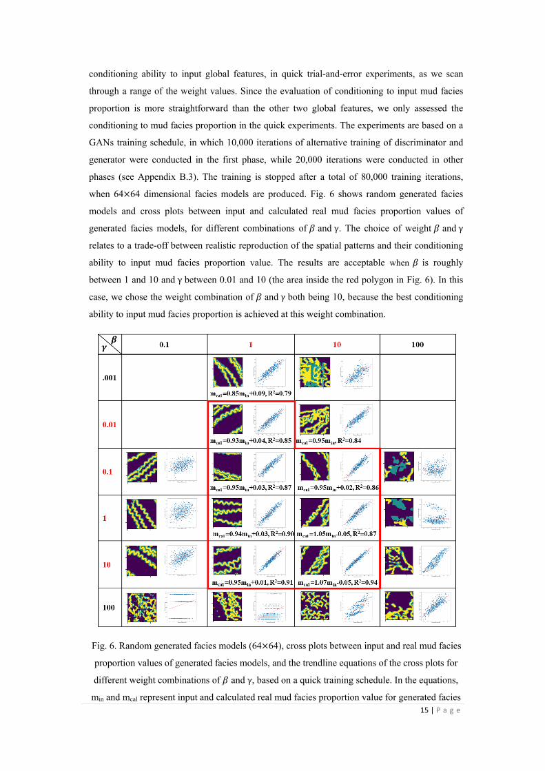
conditioning ability to input global features, in quick trial-and-error experiments, as we scan

through a range of the weight values. Since the evaluation of conditioning to input mud facies

proportion is more straightforward than the other two global features, we only assessed the

conditioning to mud facies proportion in the quick experiments. The experiments are based on a

GANs training schedule, in which 10,000 iterations of alternative training of discriminator and

generator were conducted in the first phase, while 20,000 iterations were conducted in other

phases (see Appendix B.3). The training is stopped after a total of 80,000 training iterations,

when 64×64 dimensional facies models are produced. Fig. 6 shows random generated facies

models and cross plots between input and calculated real mud facies proportion values of

generated facies models, for different combinations of 𝛽 and γ. The choice of weight 𝛽 and γ

relates to a trade-off between realistic reproduction of the spatial patterns and their conditioning

ability to input mud facies proportion value. The results are acceptable when 𝛽 is roughly

between 1 and 10 and γ between 0.01 and 10 (the area inside the red polygon in Fig. 6). In this

case, we chose the weight combination of 𝛽 and γ both being 10, because the best conditioning

ability to input mud facies proportion is achieved at this weight combination.

Fig. 6. Random generated facies models (64×64), cross plots between input and real mud facies

proportion values of generated facies models, and the trendline equations of the cross plots for

different weight combinations of 𝛽 and γ, based on a quick training schedule. In the equations,

min and mcal represent input and calculated real mud facies proportion value for generated facies

16 | P a g e

models, respectively.

The formal training schedule we used here and also in the following cases includes

20,000 training iterations for phase 1 (4×4), 40,000 training iterations for each phase during

phase 2 (8×8) to phase 4 (32×32), and unlimited number of iterations for phase 5 (64×64) until

stopping criterion is achieved (see Appendix B.3). The stopping criterion is mainly manual

inspection of the realism, diversity, and conditioning ability of generated facies models. In this

case, the GAN is trained for 13 hours, and we kept the final generator for further assessments

and practical applications. Fig. 7 shows the negative loss of the modified discriminator

(Equation (4)) versus alternative training iterations. We used the 3000 groups of global feature

values in the test dataset and randomly sampled 3000 latent vectors (from a Gaussian

distribution) to generate 3000 facies models for evaluation of the generator. Then, we arranged

the generated facies models and the 3000 real facies models in the test dataset, according to the

magnitude of the corresponding global feature values, in Fig. 8 and Fig. 9. Compared to the

facies models in the test dataset, the generated facies models are very realistic and diversified, in

spite of minor flaws.

Fig. 7. The negative loss of the modified discriminator versus training iterations

17 | P a g e

Fig. 8. Generated facies models with various input inter-channel mud proportion and channel

sinuosity index values, and ground truth test facies models with the same inter-channel mud

proportion and channel sinuosity index values. The width of channel sand is fixed at 3.1 pixels.

Fig. 9. Generated facies models with various input channel sand width and channel sinuosity index

values, and ground truth test facies models with the same channel sand width and channel

sinuosity index values. The inter-channel mud facies proportion varies from 0.51 to 0.6.

In Fig. 8 and Fig. 9, the test facies models are used as the ground truth for the generated

facies models. We see that when a certain input global feature gradually changes, the

corresponding characteristics exhibited in the generated facies models also gradually change; for

example, in the first column of Fig. 8, the mud facies proportion in the generated facies models

gradually increases, as the input inter-channel mud facies proportion value gradually increases.

18 | P a g e

In addition, the generated facies models are also very similar to the corresponding ground truth

test facies models, with respect to the mud facies proportion, the width and the sinuosity of

channel sand; for example, in Fig. 9, the upper left generated facies model is very similar to the

upper left test facies model, with respect to these characteristics.

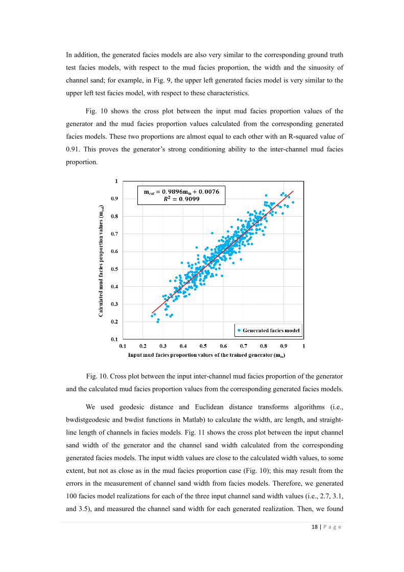
Fig. 10 shows the cross plot between the input mud facies proportion values of the

generator and the mud facies proportion values calculated from the corresponding generated

facies models. These two proportions are almost equal to each other with an R-squared value of

0.91. This proves the generator’s strong conditioning ability to the inter-channel mud facies

proportion.

Fig. 10. Cross plot between the input inter-channel mud facies proportion of the generator

and the calculated mud facies proportion values from the corresponding generated facies models.

We used geodesic distance and Euclidean distance transforms algorithms (i.e.,

bwdistgeodesic and bwdist functions in Matlab) to calculate the width, arc length, and straight-

line length of channels in facies models. Fig. 11 shows the cross plot between the input channel

sand width of the generator and the channel sand width calculated from the corresponding

generated facies models. The input width values are close to the calculated width values, to some

extent, but not as close as in the mud facies proportion case (Fig. 10); this may result from the

errors in the measurement of channel sand width from facies models. Therefore, we generated

100 facies model realizations for each of the three input channel sand width values (i.e., 2.7, 3.1,

and 3.5), and measured the channel sand width for each generated realization. Then, we found

19 | P a g e

100 facies models from the test dataset for each of the three input channel sand width values, and

measured the channel sand width for each test facies model. Fig. 12 compares the distributions

(in the form of box plot) of the channel sand width measured from the generated facies model

realizations and from the test facies models, for the three input width values. Their distributions

are very similar, indicating the generator’s strong conditioning ability to the channel sand width.

Fig. 11. The cross plot between the input channel sand width of the generator and the channel

sand width calculated from the corresponding generated facies models.

Fig. 12. The box plot of the channel sand width measured from the generated facies models and

from the test set facies models.

In this study, we use the ratio of channel arc length to straight-line length (RAS) to

represent the sinuosity of channel sand facies. Fig. 13 compares the distribution of RAS

calculated from the generated facies model realizations with that from the test setfacies models,

20 | P a g e

for each of the four input sinuosity index values (ie., 0.07, 0.23, 0.38, and 0.55). There are minor

deviations in the distribution of RAS between the generated and test set facies models when the

input sinuosity index equals 0.23 and 0.38, but generally speaking, the distributions of the RAS

for the generated and the test set facies models are very close in terms of the four input values.

This indicates the generator’s strong conditioning ability to the input channel sinuosity. To sum

up, the generator is quite robust in generating high-quality facies models and in conditioning to

the three input global features, i.e., inter-channel mud facies proportion, width and sinuosity

index of channel sand facies.

Fig. 13. The box plot of RAS of channels measured from the generated facies models and from

the test set facies models.

5.2 Conditioning to well facies data

The well facies data include two facies types (i.e., the inter-channel mud facies and the

channel complex composite facies), so the input of the generator includes one well location

indicator and one well facies indicator of the channel complex facies. The channel complex

composite facies can be generated as either the channel sand or channel bank facies in the

generated facies models. Based on the approach described in section 2.2, the number of feature

maps converted from the input well facies data is set to be 16 (Fig. 3).

In this case, we trained GANs using both the original well facies data (before well datum

enlargement) and the enlarged well facies data (after well datum enlargement), and compared the

two trained generators, in terms of the quality of the generated facies models, the well facies

reproduction accuracy, and the local pixel noise around well points.

Similar to the previous case, weight 𝜆 in the Wasserstein loss Equation (A4) is set at the

default value of 10 (Gulrajani et al. 2017), and weight 𝛽 in Equation (2) is decided based on

21 | P a g e

quick trial-and-error experiments. Fig. 16 shows random generated facies models and

reproduction accuracies of input well facies data for different 𝛽 values, in the two scenarios of

with and without input well data enlargement. The experiments suggest that the setting of 𝛽

value relates to a trade-off between the realism of the facies models and the reproduction

accuracy of input well facies data. Weight 𝛽 is suggested to be located roughly between 103 and

105.

Fig. 16. Random generated facies models (64×64) and reproduction accuracies of input well

facies data (upper is for channel complex facies and lower is for mud facies) for different weight

𝛽 based on the quick training schedule explained in section 5.1, in the two scenarios of with and

without input well data enlargement.

In our study, we set weight 𝛽 to be 103 in both scenarios. Both GANs were trained for 15

hours with 2 GPUs and 10 CPUs in parallel. Fig. 17 and Fig. 18 show the negative Wasserstein

loss with gradient penalty (W-gp loss) (Equation (2)) versus training iterations, during training

the two GANs; this loss is also called the negative critic loss in GAN research community. After

training, to evaluate the trained generators, we randomly sampled well facies data from the test

facies models, and took the sampled well facies data and random latent vectors as inputs into the

trained generators to produce facies models. Fig. 19 and Fig. 21 show some facies model

examples that are produced from the two trained generators with the same input well facies data,

and corresponding E-type and variance for channel complex facies. By manual inspection, over

90% of the generated facies models from both generators are very realistic and diversified. The

number and the configuration of the input well facies data affect the quality of the generated

facies models. At input well points, the E-type values of channel complex are very close to either

1 or 0, indicating perfect conditioning of the generated facies models to input well facies data.

The variance values at areas away from the well data are pretty close to the maximum variance

value of 0.25; this proves good diversity of the generated facies models, to a large extent.

22 | P a g e

Fig. 17. The negative W-gp loss versus training iterations, during the training of the GAN

before well datum enlargement.

Fig. 18. The negative W-gp loss versus training iterations, during the training of the GAN

after well datum enlargement.

23 | P a g e

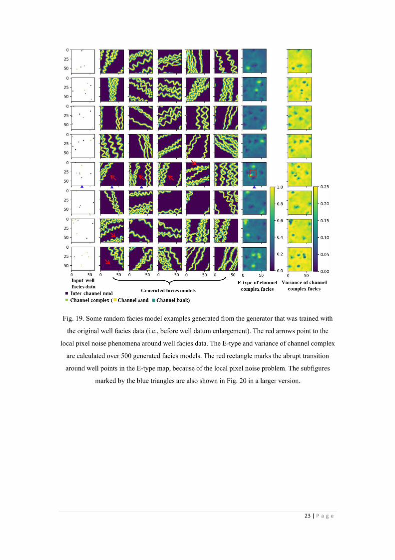
Fig. 19. Some random facies model examples generated from the generator that was trained with

the original well facies data (i.e., before well datum enlargement). The red arrows point to the

local pixel noise phenomena around well facies data. The E-type and variance of channel complex

are calculated over 500 generated facies models. The red rectangle marks the abrupt transition

around well points in the E-type map, because of the local pixel noise problem. The subfigures

marked by the blue triangles are also shown in Fig. 20 in a larger version.

24 | P a g e

Fig. 20. A large version of the input sparse well facies data, the generated facies models, and the

E-type map of channel complex marked by blue triangles in Fig. 19.

25 | P a g e

Fig. 21. Some random facies model examples generated from the generator that was trained with

the enlarged well facies data. The E-type and variance of channel complex are calculated over 500

generated facies models.

By quantitative evaluation over 3000 randomly generated facies models, the well facies

reproduction accuracies of the two generators are both 100% for both the channel complex facies

and the inter-channel mud facies. Among the facies models generated from the generator that

was trained using the original well facies data, local pixel noise problem was found in a small

group of the facies models. These areas are pointed out by the red arrows in Fig. 19, and some of

them are shown in Fig. 20 with a larger version. We also calculated the E-type map of the

channel complex for each input well facies data from 500 generated facies models (the second

last column in Fig. 19 and Fig. 21). Because of the local pixel noise problem, there are abrupt

transitions from some well points to the surrounding values in some E-type maps; one such area

is marked with the red rectangle in Fig. 19, and Fig. 20 shows a larger version of this E-type

map.

26 | P a g e

Among the facies models generated from the generator trained with the enlarged well

facies data, no local pixel noise problem was found. In the E-type maps of the channel complex,

the transitions from the well points to their surrounding values are smooth. Fig. 21 shows some

random facies models generated by enlarging and inputting the well facies data in Fig. 19.

In sum, the trained generators can generate high-quality facies models with 100% well

facies reproduction accuracy. The local pixel noise problem is addressed by using the well datum

enlargement approach. However, well datum enlargement means forcing the surrounding 4×4-

pixel area to have the same facies type as the concerning well point; this introduces an artifact

bias and reduces the uncertainty of the generated facies models to some extent. Compared to the

local pixel problem, this artifact bias may be acceptable in practical applications modeling

spatially correlated geology.

We further analyzed the generator trained with the enlarged well facies data, by

comparing the distributions of sinuosity of the generated facies models and the test facies

models. Theoretically, the two distributions should be as close as possible. Fig. 22 shows the

closeness of channel sinuosity distributions of test facies models, and generated facies models

with different input well facies conditioning data, and the aggregate of all generated facies

models. Therefore, the trained generator generates conditional facies models that captures the

distribution of sinuosity present in the training data.

Fig. 22. Channel sinuosity distributions (cdf) of test facies models, generated facies models with

27 | P a g e

different input well facies data, and the aggregate of all generated facies models.

5.3 Conditioning to both global features and well facies data

We consider two subcases: (1) conditioning to both mud facies proportion and well facies

data, and (2) conditioning to channel sinuosity and well facies data. The well facies data are

enlarged to avoid local pixel noise.

In both subcases, weight 𝜆 in the discriminator loss Equation (9) is set at the default value

of 10 (Gulrajani et al. 2017). The discriminator loss (Equation (9)) in this case is very similar to

the discriminator loss (Equation (4)) in the case of only conditioning to global features. Fig. 6

showed good performance when weight γ was between 0.1 and 10, in the case of conditioning to

global features only. Thus, γ is set to 10 here in the both subcases. The weight for global feature-

based loss and well facies-based loss, 𝛽1 and 𝛽2 in Equation (7) and (8), are decided based on

quick trial-and-error experiments. We only conducted the experiments for the first subcase (i.e.,

conditioning to mud facies proportion and well facies data). Weight 𝛽1 and 𝛽2 for the second

subcase (i.e., conditioning to channel sinuosity and well facies data) is set to be the same as the

first subcase, because both subcases share the same loss functions for the generator and the

discriminator (Equation (7), (8), and (9)). Fig. 23 shows generated facies models, cross plots

between input and real mud facies proportion value of generated facies models, and reproduction

accuracies of input well facies data, for various weight combinations of 𝛽1 and 𝛽2, in the first

subcase. The settings of weight 𝛽1 and 𝛽2 involve a trade-off among conditioning ability to input

mud facies proportion, conditioning ability to input well facies data, and realism of generated

facies models. From Fig. 23, we can conclude a rough range for weight 𝛽1 and 𝛽2: 0.05<𝛽1<0.5

and 0.25<𝛽2<25. Because normalization is applied for the three losses (i.e., the original GAN

loss, the global feature-based loss, and well facies-based loss) of the generator loss function

(Equation (7)) in this case, the magnitude of weights 𝛽1 and 𝛽2 is not comparable to the

corresponding weights in previous cases. In the both subcases, we set 𝛽1 and 𝛽2 as 0.05 and

0.25, respectively.

28 | P a g e

Fig. 23. Random generated facies models (64×64), cross plots between input and real mud

facies proportion value of generated facies models, trendline equations of the cross plots, and

reproduction accuracies of input well facies data (upper is for channel complex facies and lower

is for mud facies), for various weight combinations of 𝛽1 and 𝛽2, in the first subcase. The

trainings of GANs in this figure are based on the quick training schedule explained in section

5.1. In the equations, min and mcal represent the input and calculated real mud facies proportion

values for generated facies models.

In the first subcase, the GAN was trained for 15 hours with 2 GPUs and 10 CPUs in

parallel. Fig. 24 shows the negative loss of the modified discriminator (Equation (4)) versus

training iterations. After training, the generator takes well facies data, mud facies proportion

value, and latent vector as inputs and produces corresponding realistic facies model. Fig. 25

shows some generated facies model examples and E-type and variance for channel complex

facies, for various input mud proportion values and random well facies data sets. By manual

inspection, the generated facies models are very realistic and diversified. The variance of

channel complex in areas away from wells are close to the maximum variance value of 0.25

especially when the input mud facies proportion varies from 0.46 to 0.69, also indicating good

diversity in the generated facies models.

29 | P a g e

Fig. 24. The negative W-gp loss versus training iterations, during training of the GAN in the

subcase of conditioning to mud facies proportion and well facies data.

Fig. 25. Some random facies model examples generated from the trained generator in the

subcase of conditioning to mud facies proportion and well facies data. The second column shows

the ground truth facies models with respect to the input mud facies proportion and well facies

data. The E-type and variance of channel complex are calculated over 500 generated facies

models.

As shown in Fig. 25, the generated facies models are similar to the referenced ground truth

facies models (second column of Fig. 25) with respect to mud proportion characteristic. As the

30 | P a g e

input mud facies proportion value increases, the mud proportion of the generated facies models

also increases. In addition, we randomly generated 500 facies models, and Fig. 26 shows the

cross plot between the input mud facies proportion values into the generator and the mud facies

proportion values calculated from the corresponding generated facies models. These two

proportion values are very close with an R-squared value of 0.83. These proves the generator’s

strong conditioning ability to input mud facies proportion values, both qualitatively and

quantitatively.

Fig. 26. Cross plot between the input inter-channel mud facies proportion and the mud

facies proportion calculated from the corresponding generated facies models, when the generator

is conditioning to both mud proportion and well facies data.

In Fig. 25, the E-type values of channel complex at input well points are very close to 1 or

0. By further quantitative evaluation of 3000 randomly generated facies models, the well facies

reproduction accuracies for channel complex and inter-channel mud facies are 99.4% and

98.8%, respectively, quantitatively showing the generator’s strong conditioning ability to input

well facies data.

In the second subcase of conditioning to channel sinuosity and well facies data, the GAN

was trained for 20 hours with 2 GPUs and 10 CPUs in parallel. Fig. 27 shows the negative loss

of the modified discriminator. The trained generator takes well facies data, channel sinuosity

value, and latent vector as inputs and produces corresponding facies models. Fig. 28 shows some

generated facies model examples and E-type and variance of channel complex facies, for various

input channel sinuosity values and random well facies data. Similar to the first subcase, by

31 | P a g e

manually inspecting the generated facies models, comparing them with the corresponding

ground truth facies models, and inspecting E-type and variance maps, we can qualitatively

conclude that, the generated facies models are realistic, diversified, and conditioned to input

sinuosity values and input well facies data.

Fig. 27. The negative W-gp loss versus training iterations, during training of the GAN in the

subcase of conditioning to channel sinuosity and well facies data.

Fig. 28. Some random facies model examples generated from the trained generator in the

subcase of conditioning to channel sinuosity index values and well facies data. The second

column shows the ground truth facies models with respect to the input channel sinuosity values

and well facies data. The E-type and variance of channel complex are calculated over 500

generated facies models.

32 | P a g e

Fig. 29 compares the calculated RAS distributions of generated facies models and the

ground truth test facies models, for different input sinuosity index values. In spite of minor

deviations, the overall RAS distributions of the generated facies models are very close to that of

the test facies models for different sinuosity index values, further proving the generator’s strong

conditioning ability to the input channel sinuosity. In addition, quantitative evaluation of 3000

randomly generated facies models shows that the well facies reproduction accuracies for channel

complex facies and inter-channel mud facies are 99.6% and 97.9%, respectively, also indicating

the generator’s strong conditioning ability to input well facies data.

Fig. 29. The RAS box plot of generated facies models and the ground truth test facies models,

for different input sinuosity index values, in the subcase of conditioning to channel sinuosity and

well facies data.

We further analyzed the trained generators of the both subcases, using the distributions of

the global features that were left free and were not used for conditioning the generated facies

models. Fig. 30 compares the channel sand width distributions (cdf’s) of the test facies models

and the facies models generated by the generator of the second subcase with various input

sinuosity values. The cdf’s of the generated facies models are close to the cdf of the test ground

truth facies models. It is the similar case for channel sinuosity and mud facies proportion in both

subcases. Therefore, the two trained generators of both subcases capture the distribution of

global features that are not conditioned by input data.

33 | P a g e

Fig. 30. Channel width distributions (cdf’s) of test ground truth facies models, generated facies

models by the trained generator of the second subcase with different input sinuosity values, and

the aggregate of all generated facies models.

6. Conclusions

In the GAN-based unconditional facies modeling, researchers use the original Generative

Adversarial Networks (GANs) loss function to force the generator to learn the geological

patterns from the training facies models. To train the generator to also grasp the conditioning

ability to input conditioning data, we introduce an extra loss function into GANs, which is

defined as the inconsistency between the input conditioning value and the corresponding

characteristics exhibited by the output facies model. In addition, we design efficient architectures

for including non-spatial global features (e.g., facies ratio), sparse well facies data, and both

jointly as input conditions into the generator of the GANs. The global features are taken as

inputs by concatenating with the latent vector. To input the well facies data, first we decompose

it into multiple indicator channels, then we downsample the indicator channels into various

resolution levels, and finally we input these downsampled and the original indicator channels

into different hidden layers of the generator during the progressive growing of GANs. Such a

design allows the generator to learn the geological patterns and the conditioning ability

progressively from coarse scales to fine scales. We train GANs in a progressive growing manner,

and after training, we evaluate both the quality of generated facies models and the conditioning

ability of the generators. It turns out that the trained generators are quite robust both in

34 | P a g e

generating high-quality facies models and in conditioning to the global and local data. The

performance is not very sensitive to choice of weights for the different components of the loss

function. The reasonable ranges of predefined weights in loss functions are quite wide, with a

spread of 1 to 3 orders of magnitude. Within the range, the generated facies models are realistic,

and their conditioning to input data is excellent.

The generated facies models from current generators are in 2D. We are extending the

proposed conditional facies modeling workflow into 3D, and expect to also achieve conditioning

ability of GANs to low-resolution “soft” probability data in future work.

Acknowledgement

This work was supported by the National Science and Technology Major Projects (No.

2016ZX05014002). We acknowledge the sponsors of the Stanford Center for Earth Resources

Forecasting (SCERF) and support from Prof. Steve Graham, the Dean of the Stanford School of

Earth, Energy and Environmental Sciences. Some of the computing for this project was

performed on the Sherlock cluster. We would like to thank Stanford University and the Stanford

Research Computing Center for providing computational resources and support that contributed

to these research results. Codes, data, and some results of this work are available at the GitHub

site (https://github.com/SuihongSong/GeoModeling_Conditional_ProGAN).

References

Borji A. (2018) Pros and Cons of GAN Evaluation Measures. arXiv e-prints. arXiv:1802.03446

Chan S., Elsheikh A.H. Chan S., Elsheikh A.H. , (2017), Parametrization and generation of

geological models with generative adversarial networks

Chan S., Elsheikh A.H. (2019) Parametric generation of conditional geological realizations using

generative neural networks. Comput. Geosci. https://doi.org/10.1007/s10596-019-09850-7

Clerici A., Perego S. (2016) A Set of GRASS GIS-Based Shell Scripts for the Calculation and

Graphical Display of the Main Morphometric Parameters of a River Channel. Int. J. Geosci.

https://doi.org/10.4236/ijg.2016.72011

Dumoulin V., Belghazi I., Poole B., Mastropietro O., Lamb A., Arjovsky M., Courville A. (2016)

Adversarially Learned Inference. arXiv e-prints. arXiv:1606.00704

Dupont E., Zhang T., Tilke P., Liang L., Bailey W. (2018) Generating Realistic Geology Conditioned

on Physical Measurements with Generative Adversarial Networks. arXiv e-prints. arXiv:1802.03065

Gan Z., Henao R., Carlson D., Carin L. (2015) Learning deep sigmoid belief networks with data

augmentation. In: Journal of Machine Learning Research

Goodfellow I., Pouget-Abadie J., Mirza M., Xu B., Warde-Farley D., Ozair S., Courville A., Bengio

35 | P a g e

Y. (2014) Generative Adversarial Networks. In: Advances in Neural Information Processing Systems

27

Gulrajani I., Ahmed F., Arjovsky M., Dumoulin V., Courville A. (2017) Improved Training of

Wasserstein GANs. arXiv e-prints. arXiv:1704.00028

Ian Goodfellow, Yoshua Bengio A.C. (2015) Deep Learning.

Isola P., Zhu J.-Y., Zhou T., Efros A.A. (2016) Image-to-Image Translation with Conditional

Adversarial Networks. arXiv e-prints. arXiv:1611.07004

Karras T., Aila T., Laine S., Lehtinen J. (2017) Progressive Growing of GANs for Improved Quality,

Stability, and Variation. arXiv e-prints. arXiv:1710.10196

Karras T., Laine S., Aila T. (2018) A Style-Based Generator Architecture for Generative Adversarial

Networks. arXiv e-prints. arXiv:1812.04948

Laloy E., Hérault R., Jacques D., Linde N. (2018) Training-Image Based Geostatistical Inversion

Using a Spatial Generative Adversarial Neural Network. Water Resour. Res.

https://doi.org/10.1002/2017WR022148

Larochelle H., Murray I. (2011) The Neural Autoregressive Distribution Estimator. In: Proceedings

of the 14th International Conference on Artificial Intelligence and Statistics (AISTATS 2011)

Ledig C., Theis L., Huszar F., Caballero J., Cunningham A., Acosta A., Aitken A., Tejani A., Totz J.,

Wang Z., Shi W. (2016) Photo-Realistic Single Image Super-Resolution Using a Generative

Adversarial Network. arXiv e-prints. arXiv:1609.04802

Mirza M., Osindero S. (2014) Conditional Generative Adversarial Nets. arXiv e-prints.

arXiv:1411.1784

Mosser L., Dubrule O., Blunt M.J. (2020) Stochastic Seismic Waveform Inversion Using Generative

Adversarial Networks as a Geological Prior. Math. Geosci. https://doi.org/10.1007/s11004-019-

09832-6

Mosser L., Kimman W., Dramsch J., Purves S., De la Fuente Briceño A., Ganssle G. (2018) Rapid

seismic domain transfer: Seismic velocity inversion and modeling using deep generative neural

networks. In: 80th EAGE Conference and Exhibition 2018: Opportunities Presented by the Energy

Transition

Nesvold E., Mukerji T. (2019) Geomodeling using Generative Adversarial Networks and a database

of satellite imagery of modern river deltas. In: Petroleum Geostatistics

Van Den Oord A., Dieleman S., Zen H., Simonyan K., Vinyals O., Graves A., Kalchbrenner N.,

Senior A., Kavukcuoglu K. (2016)(a) WaveNet: A Generative Model for Raw Audio. arXiv e-prints.

arXiv:1609.03499

Van Den Oord A., Kalchbrenner N., Vinyals O., Espeholt L., Graves A., Kavukcuoglu K. (2016)(b)

Conditional image generation with PixelCNN decoders. In: Advances in Neural Information

Processing Systems

Pyrcz M.J., Deutsch C. V. (2014) Geoestatistical Reservoir Modeling.

Reed S., Akata Z., Yan X., Logeswaran L., Schiele B., Lee H. (2016) Generative Adversarial Text to

Image Synthesis. arXiv e-prints. arXiv:1605.05396

Rezende D.J., Mohamed S., Wierstra D. (2014) Stochastic backpropagation and approximate

inference in deep generative models. In: 31st International Conference on Machine Learning, ICML

2014

Sun A.Y. (2018) Discovering State-Parameter Mappings in Subsurface Models Using Generative

Adversarial Networks. Geophys. Res. Lett. https://doi.org/10.1029/2018GL080404

36 | P a g e

Zhang T.F., Tilke P., Dupont E., Zhu L.C., Liang L., Bailey W. (2019) Generating geologically

realistic 3D reservoir facies models using deep learning of sedimentary architecture with generative

adversarial networks. Pet. Sci. https://doi.org/10.1007/s12182-019-0328-4

Zhong Z., Sun A.Y., Jeong H. (2019) Predicting CO 2 Plume Migration in Heterogeneous

Formations Using Conditional Deep Convolutional Generative Adversarial Network . Water Resour.

Res. https://doi.org/10.1029/2018wr024592

Zhu J.Y., Park T., Isola P., Efros A.A. (2017) Unpaired Image-to-Image Translation Using Cycle-

Consistent Adversarial Networks. In: Proceedings of the IEEE International Conference on

Computer Vision

Zuo C., Yin Z., Pan Z., MacKie E.J., Caers J. (2020) A tree-based direct sampling method for

stochastic surface and subsurface hydrological modeling. Water Resour. Res.

https://doi.org/10.1029/2019WR026130

37 | P a g e

Appendixes

Appendix A. Introduction for GANs

A.1 GAN framework

The framework of GANs was proposed by Goodfellow et al. (2014) to address the

generative problem. Given many observed real samples 𝑥𝑟’s from an unknown distribution 𝑝𝑑𝑎𝑡𝑎

over a high-dimensional space 𝒳 , i.e., 𝑥𝑟~𝑝𝑑𝑎𝑡𝑎 , the goal of GANs is to train a generative

model that can reproduce a distribution 𝑝𝐺 to approximate 𝑝𝑑𝑎𝑡𝑎 . Fig. A1 shows the typical

workflow of a GAN. In general, a GAN includes two trainable blocks, a generator (𝐺𝜃) and a

discriminator (𝐷𝜑 ) (𝜃 and 𝜑 are trainable parameters). We define a latent variable 𝑍 with a

known distribution 𝑝𝑧 (e.g., Gaussian) over a low-dimensional space 𝒵, and define 𝑧 as a sample

from 𝑍, i.e., 𝑧~𝑝𝑧. The generator 𝐺𝜃 maps 𝑧 into a “fake” sample 𝑥𝐺 over the space 𝒳, i.e., 𝑥𝐺 =

𝐺𝜃(𝑧) ; the distribution of 𝑥𝐺 is 𝑝𝐺 , i.e., 𝑥𝐺~𝑝𝐺 . The discriminator 𝐷𝜑 maps the generated

sample 𝑥𝐺 and the given data sample 𝑥𝑟 into two scalar values, which are called scores; the two

scores are abbreviated as 𝑠𝐺 and 𝑠𝑟 , i.e., 𝑠𝐺 = 𝐷𝜑(𝑥𝐺), 𝑠𝑟 = 𝐷𝜑(𝑥𝑟). The scores evaluate the

realism of the inputs of 𝐷𝜑. The loss function of GANs is defined as some type of distance

between 𝑠𝐺 and 𝑠𝑟 (Equation (A1)); in essence, the loss represents the distance between the 𝑝𝐺

and 𝑝𝑑𝑎𝑡𝑎. We will discuss the loss function in more detail in section A.2. The discriminator 𝐷𝜑

and the generator 𝐺𝜃 are alternatively trained by maximizing and minimizing the loss (Equation

(A1)), until a certain stopping criterion is reached. In practice, usually a batch of 𝑧’s and 𝑥𝑟’s are

taken as inputs for the training of the GAN.

Fig. A1. The basic GAN framework in the context of the geological facies modeling.

min𝜃

max𝜑

𝐿(𝐺𝜃 , 𝐷𝜑) = min𝜃

max𝜑

𝔼𝑥𝐺~𝑝𝐺,𝑥𝑟~𝑝𝑑𝑎𝑡𝑎𝐷𝑖𝑠𝑡(𝑠𝐺 , 𝑠𝑟) (A1)

where, 𝐿(𝐺𝜃 , 𝐷𝜑) is the loss function, 𝐷𝑖𝑠𝑡(𝑠𝐺 , 𝑠𝑟) is some type of distance between 𝑠𝐺 and 𝑠𝑟 ,

and 𝔼 is the expectation over 𝑥𝐺~𝑝𝐺 and 𝑥𝑟~𝑝𝑑𝑎𝑡𝑎.

Fig. A2 gives an intuitive way to understand the mechanism behind GANs. For better

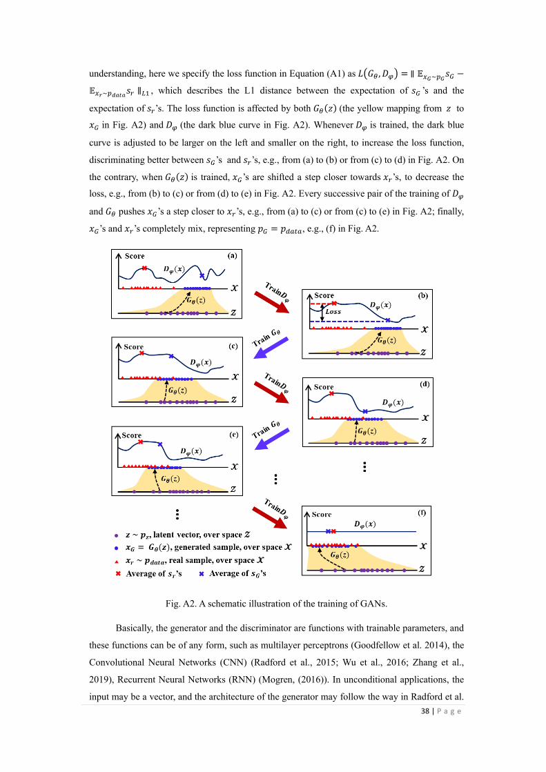
38 | P a g e

understanding, here we specify the loss function in Equation (A1) as 𝐿(𝐺𝜃 , 𝐷𝜑) = ∥ 𝔼𝑥𝐺~𝑝𝐺𝑠𝐺 −

𝔼𝑥𝑟~𝑝𝑑𝑎𝑡𝑎𝑠𝑟 ∥𝐿1 , which describes the L1 distance between the expectation of 𝑠𝐺 ’s and the

expectation of 𝑠𝑟’s. The loss function is affected by both 𝐺𝜃(𝑧) (the yellow mapping from 𝑧 to

𝑥𝐺 in Fig. A2) and 𝐷𝜑 (the dark blue curve in Fig. A2). Whenever 𝐷𝜑 is trained, the dark blue

curve is adjusted to be larger on the left and smaller on the right, to increase the loss function,

discriminating better between 𝑠𝐺’s and 𝑠𝑟’s, e.g., from (a) to (b) or from (c) to (d) in Fig. A2. On

the contrary, when 𝐺𝜃(𝑧) is trained, 𝑥𝐺’s are shifted a step closer towards 𝑥𝑟’s, to decrease the

loss, e.g., from (b) to (c) or from (d) to (e) in Fig. A2. Every successive pair of the training of 𝐷𝜑

and 𝐺𝜃 pushes 𝑥𝐺’s a step closer to 𝑥𝑟’s, e.g., from (a) to (c) or from (c) to (e) in Fig. A2; finally,

𝑥𝐺’s and 𝑥𝑟’s completely mix, representing 𝑝𝐺 = 𝑝𝑑𝑎𝑡𝑎, e.g., (f) in Fig. A2.

Fig. A2. A schematic illustration of the training of GANs.

Basically, the generator and the discriminator are functions with trainable parameters, and

these functions can be of any form, such as multilayer perceptrons (Goodfellow et al. 2014), the

Convolutional Neural Networks (CNN) (Radford et al., 2015; Wu et al., 2016; Zhang et al.,

2019), Recurrent Neural Networks (RNN) (Mogren, (2016)). In unconditional applications, the

input may be a vector, and the architecture of the generator may follow the way in Radford et al.

39 | P a g e

(2015). In some conditional applications, if the input is high-dimensional data, like images, then

the architecture of the generator may follow a “U-Net” design, as in Ledig et al. (2016). The

architecture design of the generator and the discriminator can be very complicated in some

applications (e.g., Ma et al., 2017; H. Zhang et al., 2016).

A.2 GAN Loss

Since the GAN framework was proposed, many different types of loss functions have been

studied (Lucic et al. 2017), and each of them corresponds to a type of distance between 𝑝𝐺 and

𝑝𝑑𝑎𝑡𝑎.

Originally, Goodfellow et al. (2014) proposed the loss function given below in Equation

(A2), where the last layer of 𝐷𝜑 is a sigmoid function.

𝐿(𝐺𝜃 , 𝐷𝜑) = 𝔼𝑥𝑟~𝑝𝑑𝑎𝑡𝑎[𝑙𝑜𝑔𝐷𝜑(𝑥𝑟)] + 𝔼𝑧~𝑝𝑧

[log (1 − 𝐷𝜑(𝐺𝜃(𝑧)))] (A2)

this loss function was proved to be equivalent to being a Jensen-Shannon divergence between

𝑝𝑑𝑎𝑡𝑎 and 𝑝𝐺 (Goodfellow et al. 2014).

Arjovsky et al. (2017) showed that the Wasserstein distance is more sensitive than the

Jensen-Shannon divergence, and proposed the Wasserstein loss function based on the

Wasserstein distance between 𝑝𝑑𝑎𝑡𝑎 and 𝑝𝐺 (Equation (A3)).

𝐿(𝐺𝜃 , 𝐷𝜑) = 𝔼𝑥𝑟~𝑝𝑑𝑎𝑡𝑎𝐷𝜑(𝑥𝑟) − 𝔼𝑧~𝑝𝑧

𝐷𝜑(𝐺𝜃(𝑧)) (A3)

where 𝐷𝜑 does not have the sigmoid function in the last layer and should be changing slowly.

Gulrajani et al. (2017) improved the Wasserstein loss function by using a gradient penalty

to enforce the gradient of 𝐷𝜑 to be small. This improved loss function is shown in Equation

(A4).

𝐿(𝐺𝜃 , 𝐷𝜑) = 𝔼𝑥𝑟~𝑝𝑑𝑎𝑡𝑎𝐷𝜑(𝑥𝑟) − 𝔼𝑧~𝑝𝑧

𝐷𝜑(𝐺𝜃(𝑧)) − 𝜆𝔼�̂�~𝑝�̂�[(∥ ∇�̂�𝐷𝜑(�̂�) ∥2− 1)2] (A4)

where, 𝐷𝜑 does not have the sigmoid function in the last layer, 𝜆 is a predefined weight, and �̂� is

sampled between 𝑥𝑟~𝑝𝑑𝑎𝑡𝑎 and 𝑥𝐺~𝑝𝐺 using 𝑡~𝑢𝑛𝑖𝑓𝑜𝑟𝑚(0,1), i.e., �̂� = 𝑡𝑥 + (1 − 𝑡)𝑥𝐺.

Appendix B. Unconditional facies modeling using

progressive growing of GANs

B.1 GAN Architectures

The facies model is spatially correlated, so we use Convolutional Neural Network (CNN)

40 | P a g e

for both the generator and the discriminator. The architecture of the generator is shown in Fig.

B1 and Table B1. The input of the generator is a 128×1 latent vector that is sampled from a

standard Gaussian distribution, i.e., 𝑧~𝐺𝑎𝑢𝑠𝑠𝑖𝑎𝑛(0,1); the output is a 64×64 facies model. The

architecture of the generator includes 1 fully connected neural network layer with 128 input

neurons and 2048 output neurons, 1 reshape layer, 4 upsampling layers, and 10 2-dimensional

convolutional layers. The reshape layer converts the 2048×1 vector into the 4×4×128 feature

cube, corresponding to 128 feature maps of size 4×4. Each upsampling layer dilates the heights

and widths of the feature cubes by 2, using the nearest-neighbor upsampling method. The kernel

size for the last convolution layer is 1×1, while the kernel size for the other convolutional layers

is 3×3; the stride size for all convolutional layers is 1×1. The leaky rectified linear unit function

(LReLU) with a leaky value of 0.2 is used as the activation function in all hidden layers except

the last for which a linear activation function is used. As seen in Fig. B1 and Table B1, the

architecture consists of five blocks of layers producing feature maps with coarser to finer

resolution – 4×4, 8×8, 16×16, and 32×32, and finally 64×64. The first fully connected layer is

also included in block 1 (4×4) for easier description. These five blocks are trained progressively

starting from the coarse 4×4 block to finer and finer blocks ending with 64×64 output image.

The progressive training process is described in more detail later.

The architecture of the discriminator is essentially symmetrical to the generator, with

corresponding blocks of layers producing feature maps with coarse (4×4) to increasingly fine

resolution (8×8, 16×16, 32×32, and 64×64), except that the output of the discriminator is a

scalar and a minibatch standard deviation layer (discussed below) is applied at the discriminator

(Fig. B1 and Table B1). The kernel size for the first convolutional layer is 1×1, while the kernel

size for the other convolutional layers is 3×3. The minibatch standard deviation technique was

proposed by Karras et al. (2017) to increase the variation of the generated results. The

calculation steps for the minibatch standard deviation layer are as follows (Fig. B2): first,

calculate the standard deviation for each feature map at each spatial location over the minibatch;

second, average these calculated standard deviation values over all feature maps and spatial

locations to obtain a single value; third, replicate the value into an additional feature map with

the same resolution as other feature maps; finally, concatenate the new feature map with other

feature maps of the minibatch, and this increases the channels (or the number of feature maps)

by one, from 128 to 129 after the minibatch standard deviation layer (MSD in Fig. B1). This

layer could be inserted anywhere in the discriminator, but it is best to be inserted towards the end

(Karras et al., 2017).

41 | P a g e

Fig. B1. The architectures of the generator and the discriminator used in this study.

Fig. B2. Illustration of how a minibatch standard deviation layer works.

Table B1. The detailed architectures of the generator and the discriminator used in this study

B.2 Loss function training

We use the Wasserstein loss function with gradient penalty (W-gp). During the training,

the trainable parameters (i.e., 𝜃 and 𝜑) are initialized with He initialization approach (He et al.

2015). To speed up the training process, the minibatch gradient descent and the Adam optimizer

42 | P a g e

(Kingma and Ba, 2014) with the default parameters are used. Every minibatch is set to include

32 facies models. In many studies, the number of optimization times for the discriminator in

each loop is set to be larger than 1, i.e., researchers alternate between multiple times of

optimizing the discriminator and one time of optimizing the generator; we set the optimization

times of the discriminator to be 1 in each loop, because the Wasserstein loss can largely stabilize

the training process.

B.3 Progressive training process

The training of GANs is actually a process of forcing the generator to learn all the features

of given samples, and the features have various scales. In most GAN related researches, the

scales of features are not considered and all layers of GANs are trained concurrently, so the

generator has to manage and learn different scales of features completely by itself; this may

result in an inefficient way of feature learning of the generator, e.g., some fine-scale features

may be learned earlier than the large-scale features. Therefore, Karras et al. (2017) proposed a

new training methodology for GANs: the progressive growing of GANs or the progressive

training process, in which the generator and the discriminator are trained layer by layer. The

shallower layers of the generator learn the larger-scale features of the given samples, while the

deeper layers of the generator learn the finer-scale features. Karras et al. (2017) has proved that

the progressive growing of GANs can speed up the training process by 2-6 times, largely

stabilize the training process, and generate better-quality results, compared to the conventional

training process.

We use the progressive training process in our study (Fig. B3). We downsample the

original 64×64-size training facies models into 32×32, 16×16, 8×8, and 4×4-size training

facies models, using averaging. These downsampled facies models and the original ones are

used during the following process.

The layers of the generator and the discriminator are progressively trained block by block

from coarse to fine (shallow to deep), in different phases. In phase 1, we activate the layers of

block 1 (4 × 4) in the generator and the discriminator (Fig. B3), and add two additional

convolutional layers (i.e., “CV(1×1)” in Fig. B3). The two convolutional layers convert the

output (the 4×4×128 feature cube) of block 1 in the generator into a 4×4 facies model and

convert a 4×4 facies model, either a training or a generated facies model, into a 4×4×128

feature cube as the input of block 1 in the discriminator. The involved layers are initialized from

scratch. We train the activated layers in this phase with 4×4-size training facies models. After

training, the largest-scale features represented by the 4×4-size training facies models are learned

by the layers of block 1 in the generator.

43 | P a g e

In phase 2, we now activate the layers of block 2 (8 × 8) in the generator and the

discriminator, and add two new convolutional layers (“CV(1×1)” in Fig. B3) that convert the

output (8×8×128 feature cube) of block 2 in the generator into a 8×8 facies model and

correspondingly convert a 8×8 facies model into a 8×8×128 feature cube. To avoid disrupting

the already trained layers in the previous phase, the newly activated layers (block 2) are included

smoothly in the generator and the discriminator by a weighted average, meaning that the

contribution of the new layers increases gradually from 0 to 1. We upsample the 4×4 facies

model generated from block 1 in the generator into a 8×8 facies model, and average that 8×8

facies model from block 1 with the 8×8 facies model converted from the output of block 2, with

a weighting factor α. The generator output now is thus (1-α) × (upsampled 8×8 facies model

from block 1) +α ×(8×8 facies model from block 2). In the discriminator, the input 8×8 facies

model, either a training or a generated facies model, is both directly converted into a 8×8×128

feature cube and downsampled into a 4×4 facies model. Block 2 in the discriminator takes that

8×8×128 feature cube as input and generates a 4×4×128 feature cube. At the same time, the

downsampled 4 × 4 facies model is converted into another 4 × 4 × 128 feature cube by a

convolutional layer. These two 4×4×128 feature cubes are then averaged into a new 4×4×128

feature cube with the same weight α, i.e., (1-α) × (4×4×128 feature cube converted from 4×4

facies model)+α ×(4×4×128 feature cube generated from block 2). This new 4×4×128 feature

cube finally goes through the layers of block 1 in the discriminator to output the score. The

weighting factor α represents the contribution of the newly activated layers of block 2. It first

changes linearly from 0 to 1, to ensure that the newly activated layers fade in smoothly without

breaking the already learned features stored in the previous block. After that, α is held constant

at 1. This allows training of all parameters (in the newly activated block as well as the previous

block) to the same degree, to enhance the robustness of the generator and the discriminator. In

this phase, the trainable parameters of the newly activated and newly added layers are initialized

from scratch, while the other trainable parameters are initialized from the values they reached in

the previous training phase. Finally, we train all the activated layers in this phase with 8×8-size

training facies models. After training, the features represented by the 8×8-size training facies

models are learned by the layers of block 2 in the generator.

In a similar manner as in phase 2, we progressively train more and more blocks of layers in

phase 3 (16×16), phase 4 (32×32), and phase 5 (64×64) until all layers in the generator and the

discriminator are trained. All scales of features of the original training facies models are learned

by these trained layers in the generator.

44 | P a g e

Fig. B3. The progressive GAN training workflow used in this study.

References

Arjovsky M., Chintala S., Bottou L. (2017) Wasserstein GAN. arXiv e-prints. arXiv:1701.07875

Goodfellow I., Pouget-Abadie J., Mirza M., Xu B., Warde-Farley D., Ozair S., Courville A., Bengio Y.

(2014) Generative Adversarial Networks. In: Advances in Neural Information Processing Systems 27

Gulrajani I., Ahmed F., Arjovsky M., Dumoulin V., Courville A. (2017) Improved Training of

Wasserstein GANs. arXiv e-prints. arXiv:1704.00028

He K., Zhang X., Ren S., Sun J. (2015) Delving Deep into Rectifiers: Surpassing Human-Level

Performance on ImageNet Classification. In: IEEE International Conference on Computer Vision. pp.

1026–1034

Karras T., Aila T., Laine S., Lehtinen J. (2017) Progressive Growing of GANs for Improved Quality,

Stability, and Variation. arXiv e-prints. arXiv:1710.10196

Kingma D., Ba J. (2014) Adam: a method for stochastic optimization. arXiv Prepr. arXiv1412.6980.

https://doi.org/10.1109/ICCE.2017.7889386

Ledig C., Theis L., Huszar F., Caballero J., Cunningham A., Acosta A., Aitken A., Tejani A., Totz J.,

Wang Z., Shi W. (2016) Photo-Realistic Single Image Super-Resolution Using a Generative

Adversarial Network. arXiv e-prints. arXiv:1609.04802

Lucic M., Kurach K., Michalski M., Gelly S., Bousquet O. (2017) Are GANs Created Equal? A Large-

Scale Study. arXiv e-prints. arXiv:1711.10337

Ma L., Jia X., Sun Q., Schiele B., Tuytelaars T., Van Gool L. (2017) Pose Guided Person Image

Generation. arXiv e-prints. arXiv:1705.09368

Mogren O. (2016) C-RNN-GAN: Continuous recurrent neural networks with adversarial training.

arXiv e-prints. arXiv:1611.09904

Radford A., Metz L., Chintala S. (2015) Unsupervised Representation Learning with Deep

Convolutional Generative Adversarial Networks. arXiv e-prints. arXiv:1511.06434

Wu J., Zhang C., Xue T., Freeman W.T., Tenenbaum J.B. (2016) Learning a Probabilistic Latent Space

of Object Shapes via 3D Generative-Adversarial Modeling. arXiv e-prints. arXiv:1610.07584

45 | P a g e

Zhang H., Xu T., Li H., Zhang S., Wang X., Huang X., Metaxas D. (2016) StackGAN: Text to Photo-

realistic Image Synthesis with Stacked Generative Adversarial Networks. arXiv e-prints.

arXiv:1612.03242

Zhang T.F., Tilke P., Dupont E., Zhu L.C., Liang L., Bailey W. (2019) Generating geologically realistic

3D reservoir facies models using deep learning of sedimentary architecture with generative adversarial

networks. Pet. Sci. https://doi.org/10.1007/s12182-019-0328-4