University of Calgary

PRISM: University of Calgary's Digital Repository

Graduate Studies The Vault: Electronic Theses and Dissertations

2021-01-14

Conceptual Design and Optimization of Hybrid

Rockets

Messinger, Troy Leonard

Messinger, T. L. (2021). Conceptual Design and Optimization of Hybrid Rockets (Unpublished

master's thesis). University of Calgary, Calgary, AB.

http://hdl.handle.net/1880/113011

master thesis

University of Calgary graduate students retain copyright ownership and moral rights for their

thesis. You may use this material in any way that is permitted by the Copyright Act or through

licensing that has been assigned to the document. For uses that are not allowable under

copyright legislation or licensing, you are required to seek permission.

Downloaded from PRISM: https://prism.ucalgary.ca

UNIVERSITY OF CALGARY

Conceptual Design and Optimization of Hybrid Rockets

by

Troy Leonard Messinger

A THESIS

SUBMITTED TO THE FACULTY OF GRADUATE STUDIES

IN PARTIAL FULFILLMENT OF THE REQUIREMENTS FOR THE

DEGREE OF MASTER OF SCIENCE

GRADUATE PROGRAM IN MECHANICAL ENGINEERING

CALGARY, ALBERTA

JANUARY, 2021

© Troy Leonard Messinger 2021

Abstract

A framework was developed to perform conceptual multi-disciplinary design parametric

and optimization studies of single-stage sub-orbital flight vehicles, and two-stage-to-orbit

flight vehicles, that employ hybrid rocket engines as the principal means of propulsion. The

framework was written in the Python programming language and incorporates many sub-

disciplines to generate vehicle designs, model the relevant physics, and analyze flight perfor-

mance. The relative performance (payload fraction capability) of different vehicle masses and

feed system/propellant configurations was found. The major findings include conceptually

viable pressure-fed and electric pump-fed two-stage-to-orbit configurations taking advan-

tage of relatively low combustion pressures in increasing overall performance. The smallest

launch vehicles assessed had lower payload fractions compared to larger vehicles. The vehi-

cle configurations resulting in the highest performance used liquid oxygen and paraffin wax

propellants. The smallest viable orbital launch vehicle, the vehicle with the highest payload

fraction for the smallest payload considered, was a liquid oxygen and paraffin-wax-based

launcher. The highest payload fraction found for the smallest payload class was 0.60 % of

gross mass for a 10 kg payload delivered to 500 km Sun-synchronous orbit. The highest pay-

load fraction for the investigated 150 kg payload class for the same Sun-synchronous orbit

was found to be 1.2 %.

ii

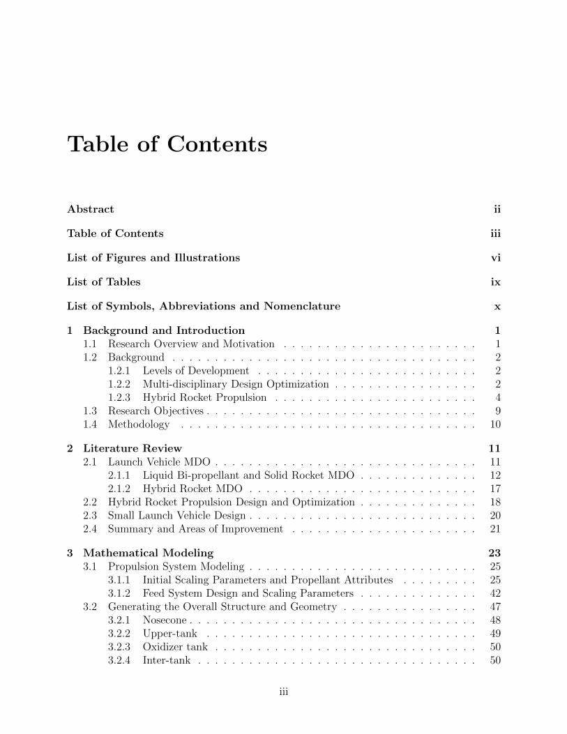
Table of Contents

Abstract ii

Table of Contents iii

List of Figures and Illustrations vi

List of Tables ix

List of Symbols, Abbreviations and Nomenclature x

1 Background and Introduction 11.1 Research Overview and Motivation . . . . . . . . . . . . . . . . . . . . . . . 11.2 Background . . . . . . . . . . . . . . . . . . . . . . . . . . . . . . . . . . . . 2

1.2.1 Levels of Development . . . . . . . . . . . . . . . . . . . . . . . . . . 21.2.2 Multi-disciplinary Design Optimization . . . . . . . . . . . . . . . . . 21.2.3 Hybrid Rocket Propulsion . . . . . . . . . . . . . . . . . . . . . . . . 4

1.3 Research Objectives . . . . . . . . . . . . . . . . . . . . . . . . . . . . . . . . 91.4 Methodology . . . . . . . . . . . . . . . . . . . . . . . . . . . . . . . . . . . 10

2 Literature Review 112.1 Launch Vehicle MDO . . . . . . . . . . . . . . . . . . . . . . . . . . . . . . . 11

2.1.1 Liquid Bi-propellant and Solid Rocket MDO . . . . . . . . . . . . . . 122.1.2 Hybrid Rocket MDO . . . . . . . . . . . . . . . . . . . . . . . . . . . 17

2.2 Hybrid Rocket Propulsion Design and Optimization . . . . . . . . . . . . . . 182.3 Small Launch Vehicle Design . . . . . . . . . . . . . . . . . . . . . . . . . . . 202.4 Summary and Areas of Improvement . . . . . . . . . . . . . . . . . . . . . . 21

3 Mathematical Modeling 233.1 Propulsion System Modeling . . . . . . . . . . . . . . . . . . . . . . . . . . . 25

3.1.1 Initial Scaling Parameters and Propellant Attributes . . . . . . . . . 253.1.2 Feed System Design and Scaling Parameters . . . . . . . . . . . . . . 42

3.2 Generating the Overall Structure and Geometry . . . . . . . . . . . . . . . . 473.2.1 Nosecone . . . . . . . . . . . . . . . . . . . . . . . . . . . . . . . . . . 483.2.2 Upper-tank . . . . . . . . . . . . . . . . . . . . . . . . . . . . . . . . 493.2.3 Oxidizer tank . . . . . . . . . . . . . . . . . . . . . . . . . . . . . . . 503.2.4 Inter-tank . . . . . . . . . . . . . . . . . . . . . . . . . . . . . . . . . 50

iii

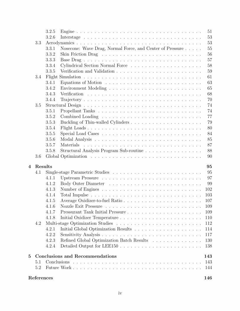
3.2.5 Engine . . . . . . . . . . . . . . . . . . . . . . . . . . . . . . . . . . . 513.2.6 Interstage . . . . . . . . . . . . . . . . . . . . . . . . . . . . . . . . . 53

3.3 Aerodynamics . . . . . . . . . . . . . . . . . . . . . . . . . . . . . . . . . . . 533.3.1 Nosecone: Wave Drag, Normal Force, and Center of Pressure . . . . . 553.3.2 Skin Friction Drag . . . . . . . . . . . . . . . . . . . . . . . . . . . . 563.3.3 Base Drag . . . . . . . . . . . . . . . . . . . . . . . . . . . . . . . . . 573.3.4 Cylindrical Section Normal Force . . . . . . . . . . . . . . . . . . . . 583.3.5 Verification and Validation . . . . . . . . . . . . . . . . . . . . . . . . 59

3.4 Flight Simulation . . . . . . . . . . . . . . . . . . . . . . . . . . . . . . . . . 613.4.1 Equations of Motion . . . . . . . . . . . . . . . . . . . . . . . . . . . 633.4.2 Environment Modeling . . . . . . . . . . . . . . . . . . . . . . . . . . 653.4.3 Verification . . . . . . . . . . . . . . . . . . . . . . . . . . . . . . . . 683.4.4 Trajectory . . . . . . . . . . . . . . . . . . . . . . . . . . . . . . . . . 70

3.5 Structural Design . . . . . . . . . . . . . . . . . . . . . . . . . . . . . . . . . 743.5.1 Propellant Tanks . . . . . . . . . . . . . . . . . . . . . . . . . . . . . 743.5.2 Combined Loading . . . . . . . . . . . . . . . . . . . . . . . . . . . . 773.5.3 Buckling of Thin-walled Cylinders . . . . . . . . . . . . . . . . . . . . 793.5.4 Flight Loads . . . . . . . . . . . . . . . . . . . . . . . . . . . . . . . . 803.5.5 Special Load Cases . . . . . . . . . . . . . . . . . . . . . . . . . . . . 843.5.6 Modal Analysis . . . . . . . . . . . . . . . . . . . . . . . . . . . . . . 853.5.7 Materials . . . . . . . . . . . . . . . . . . . . . . . . . . . . . . . . . 873.5.8 Structural Analysis Program Sub-routine . . . . . . . . . . . . . . . . 88

3.6 Global Optimization . . . . . . . . . . . . . . . . . . . . . . . . . . . . . . . 90

4 Results 954.1 Single-stage Parametric Studies . . . . . . . . . . . . . . . . . . . . . . . . . 95

4.1.1 Upstream Pressure . . . . . . . . . . . . . . . . . . . . . . . . . . . . 974.1.2 Body Outer Diameter . . . . . . . . . . . . . . . . . . . . . . . . . . 994.1.3 Number of Engines . . . . . . . . . . . . . . . . . . . . . . . . . . . . 1024.1.4 Total Impulse . . . . . . . . . . . . . . . . . . . . . . . . . . . . . . . 1034.1.5 Average Oxidizer-to-fuel Ratio . . . . . . . . . . . . . . . . . . . . . . 1074.1.6 Nozzle Exit Pressure . . . . . . . . . . . . . . . . . . . . . . . . . . . 1094.1.7 Pressurant Tank Initial Pressure . . . . . . . . . . . . . . . . . . . . . 1094.1.8 Initial Oxidizer Temperature . . . . . . . . . . . . . . . . . . . . . . . 110

4.2 Multi-stage Optimization Studies . . . . . . . . . . . . . . . . . . . . . . . . 1124.2.1 Initial Global Optimization Results . . . . . . . . . . . . . . . . . . . 1144.2.2 Sensitivity Analysis . . . . . . . . . . . . . . . . . . . . . . . . . . . . 1174.2.3 Refined Global Optimization Batch Results . . . . . . . . . . . . . . 1304.2.4 Detailed Output for LEE150 . . . . . . . . . . . . . . . . . . . . . . . 138

5 Conclusions and Recommendations 1435.1 Conclusions . . . . . . . . . . . . . . . . . . . . . . . . . . . . . . . . . . . . 1435.2 Future Work . . . . . . . . . . . . . . . . . . . . . . . . . . . . . . . . . . . . 144

References 146

iv

A Beam Element Mass and Stiffness Matrices 157

B Input Constants 158

C LEE150 Supplementary Output 161C.1 Mission Plots . . . . . . . . . . . . . . . . . . . . . . . . . . . . . . . . . . . 161C.2 Code Outputs . . . . . . . . . . . . . . . . . . . . . . . . . . . . . . . . . . . 165

v

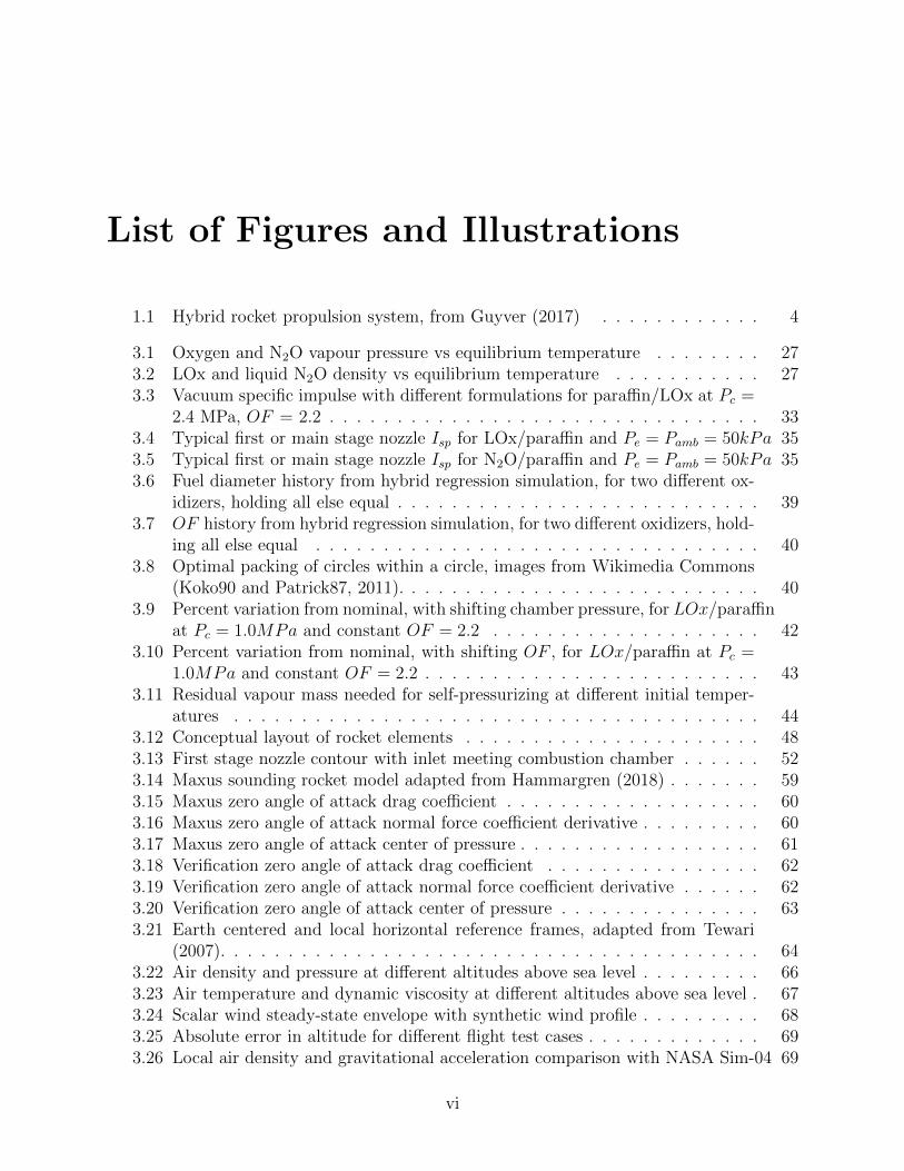
List of Figures and Illustrations

1.1 Hybrid rocket propulsion system, from Guyver (2017) . . . . . . . . . . . . 4

3.1 Oxygen and N2O vapour pressure vs equilibrium temperature . . . . . . . . 273.2 LOx and liquid N2O density vs equilibrium temperature . . . . . . . . . . . 273.3 Vacuum specific impulse with different formulations for paraffin/LOx at Pc =

2.4 MPa, OF = 2.2 . . . . . . . . . . . . . . . . . . . . . . . . . . . . . . . . 333.4 Typical first or main stage nozzle Isp for LOx/paraffin and Pe = Pamb = 50kPa 353.5 Typical first or main stage nozzle Isp for N2O/paraffin and Pe = Pamb = 50kPa 353.6 Fuel diameter history from hybrid regression simulation, for two different ox-

idizers, holding all else equal . . . . . . . . . . . . . . . . . . . . . . . . . . . 393.7 OF history from hybrid regression simulation, for two different oxidizers, hold-

ing all else equal . . . . . . . . . . . . . . . . . . . . . . . . . . . . . . . . . 403.8 Optimal packing of circles within a circle, images from Wikimedia Commons

(Koko90 and Patrick87, 2011). . . . . . . . . . . . . . . . . . . . . . . . . . . 403.9 Percent variation from nominal, with shifting chamber pressure, for LOx/paraffin

at Pc = 1.0MPa and constant OF = 2.2 . . . . . . . . . . . . . . . . . . . . 423.10 Percent variation from nominal, with shifting OF , for LOx/paraffin at Pc =

1.0MPa and constant OF = 2.2 . . . . . . . . . . . . . . . . . . . . . . . . . 433.11 Residual vapour mass needed for self-pressurizing at different initial temper-

atures . . . . . . . . . . . . . . . . . . . . . . . . . . . . . . . . . . . . . . . 443.12 Conceptual layout of rocket elements . . . . . . . . . . . . . . . . . . . . . . 483.13 First stage nozzle contour with inlet meeting combustion chamber . . . . . . 523.14 Maxus sounding rocket model adapted from Hammargren (2018) . . . . . . . 593.15 Maxus zero angle of attack drag coefficient . . . . . . . . . . . . . . . . . . . 603.16 Maxus zero angle of attack normal force coefficient derivative . . . . . . . . . 603.17 Maxus zero angle of attack center of pressure . . . . . . . . . . . . . . . . . . 613.18 Verification zero angle of attack drag coefficient . . . . . . . . . . . . . . . . 623.19 Verification zero angle of attack normal force coefficient derivative . . . . . . 623.20 Verification zero angle of attack center of pressure . . . . . . . . . . . . . . . 633.21 Earth centered and local horizontal reference frames, adapted from Tewari

(2007). . . . . . . . . . . . . . . . . . . . . . . . . . . . . . . . . . . . . . . . 643.22 Air density and pressure at different altitudes above sea level . . . . . . . . . 663.23 Air temperature and dynamic viscosity at different altitudes above sea level . 673.24 Scalar wind steady-state envelope with synthetic wind profile . . . . . . . . . 683.25 Absolute error in altitude for different flight test cases . . . . . . . . . . . . . 693.26 Local air density and gravitational acceleration comparison with NASA Sim-04 69

vi

3.27 Simulated altitude and longitude comparison with NASA Sim-04 . . . . . . . 703.28 Elliptical pressure vessel head coordinates . . . . . . . . . . . . . . . . . . . 763.29 Comparison of oxidizer tank design mass to theoretical scaling estimate . . . 783.30 Axial, lateral, bending moment, and internal pressure loads on a generic rocket

element cylinder . . . . . . . . . . . . . . . . . . . . . . . . . . . . . . . . . . 783.31 Rocket element-by-element load formulation . . . . . . . . . . . . . . . . . . 823.32 Rocket global free-body diagram . . . . . . . . . . . . . . . . . . . . . . . . . 833.33 Beam element coordinates, from Gavin (2018) . . . . . . . . . . . . . . . . . 863.34 Structural optimization program schematic . . . . . . . . . . . . . . . . . . . 913.35 Global program schematic . . . . . . . . . . . . . . . . . . . . . . . . . . . . 93

4.1 Vehicle performance (delivered ∆V ) vs chamber pressure . . . . . . . . . . . 984.2 Vehicle delivered specific impulse and propellant mass percentage vs chamber

pressure . . . . . . . . . . . . . . . . . . . . . . . . . . . . . . . . . . . . . . 994.3 Vehicle performance (delivered ∆V ) vs outer diameter . . . . . . . . . . . . 1004.4 Vehicle delivered specific impulse vs outer diameter . . . . . . . . . . . . . . 1014.5 Propellant mass percentage vs outer diameter . . . . . . . . . . . . . . . . . 1014.6 Vehicle performance (delivered ∆V ) vs number of engines . . . . . . . . . . . 1024.7 Propellant mass percentage vs number of engines . . . . . . . . . . . . . . . 1034.8 Vehicle delivered specific impulse vs number of engines . . . . . . . . . . . . 1044.9 Vehicle total liftoff mass vs total impulse . . . . . . . . . . . . . . . . . . . . 1054.10 Vehicle performance (delivered ∆V ) vs total impulse . . . . . . . . . . . . . 1054.11 Propellant mass percentage vs total impulse . . . . . . . . . . . . . . . . . . 1064.12 Vehicle delivered specific impulse vs total impulse . . . . . . . . . . . . . . . 1064.13 Vehicle performance (delivered ∆V ) vs OFav . . . . . . . . . . . . . . . . . . 1074.14 Propellant mass percentage vs OFav . . . . . . . . . . . . . . . . . . . . . . . 1084.15 Vehicle delivered specific impulse vs OFav . . . . . . . . . . . . . . . . . . . 1084.16 Vehicle performance (delivered ∆V ) and Isp vs nozzle exit pressure . . . . . 1094.17 Vehicle performance (delivered ∆V ) and propellant mass ratio vs pressurant

initial pressure . . . . . . . . . . . . . . . . . . . . . . . . . . . . . . . . . . 1104.18 Propellant mass percentage vs oxidizer initial temperature . . . . . . . . . . 1114.19 Convergence of global optimization optimization variables for LEB150 case . 1154.20 Convergence of global optimization cost function for LEB150 case . . . . . . 1164.21 Multi-stage payload fraction sensitivity to first stage upstream pressure . . . 1184.22 Multi-stage payload fraction sensitivity to second stage upstream pressure . . 1194.23 Multi-stage payload fraction sensitivity to first stage burn time . . . . . . . . 1204.24 Multi-stage payload fraction sensitivity to second stage burn time . . . . . . 1214.25 Multi-stage payload fraction sensitivity to first stage OFav . . . . . . . . . . 1224.26 Multi-stage payload fraction sensitivity to second stage OFav . . . . . . . . . 1234.27 Multi-stage payload fraction sensitivity to second stage nozzle clearance . . . 1234.28 Multi-stage payload fraction sensitivity to second stage δnozzle . . . . . . . . 1244.29 Multi-stage payload fraction sensitivity to Body OD . . . . . . . . . . . . . 1254.30 Multi-stage payload fraction sensitivity to initial pressurant gas pressure . . 1264.31 Multi-stage payload fraction sensitivity to combustion efficiency . . . . . . . 1264.32 Multi-stage payload fraction sensitivity to electric pump efficiency . . . . . . 127

vii

4.33 Multi-stage payload fraction sensitivity to electric battery multiplier . . . . . 1284.34 Multi-stage payload fraction sensitivity to structural index . . . . . . . . . . 1294.35 Multi-stage payload fraction sensitivity to first stage additional mass . . . . 1304.36 LEE150 Monte Carlo % payload distribution . . . . . . . . . . . . . . . . . . 1314.37 LBB150 Monte Carlo % payload distribution . . . . . . . . . . . . . . . . . . 1324.38 LEE150 convergence using [c1 : 1.5, c2 : 1.5, w : 0.25] . . . . . . . . . . . . . 1354.39 Altitude vs Downrange distance for LEE150 . . . . . . . . . . . . . . . . . . 1394.40 Altitude vs time for LEE150 . . . . . . . . . . . . . . . . . . . . . . . . . . . 1404.41 Velocity vs time for LEE150 . . . . . . . . . . . . . . . . . . . . . . . . . . . 1414.42 Acceleration vs time for LEE150 . . . . . . . . . . . . . . . . . . . . . . . . . 141

C.1 Initial elliptic orbit path for LEE150 . . . . . . . . . . . . . . . . . . . . . . 162C.2 Upper stage remaining ∆V vs time since first stage ignition, for LEE150 . . 162C.3 Total mass vs time for LEE150 . . . . . . . . . . . . . . . . . . . . . . . . . 163C.4 Specific impulse vs time into burn for LEE150 . . . . . . . . . . . . . . . . . 163C.5 Local flight heading, γ, vs time for LEE150 . . . . . . . . . . . . . . . . . . . 164C.6 Dynamic pressure, q, vs time for LEE150 . . . . . . . . . . . . . . . . . . . . 164

viii

List of Tables

1.1 Start-up & established companies active in the hybrid rocket propulsion field 6

3.1 Paraffin fuel attributes . . . . . . . . . . . . . . . . . . . . . . . . . . . . . . 263.2 Minimum outer diameter for packing various equal diameter circles . . . . . 413.3 Electric pump constants . . . . . . . . . . . . . . . . . . . . . . . . . . . . . 473.4 Initial valve scaling constants used . . . . . . . . . . . . . . . . . . . . . . . 503.5 Element matrix information . . . . . . . . . . . . . . . . . . . . . . . . . . . 873.6 Material properties of rocket structures . . . . . . . . . . . . . . . . . . . . . 883.7 Particle swarm optimization parameters used . . . . . . . . . . . . . . . . . . 92

4.1 Parameter nominal values . . . . . . . . . . . . . . . . . . . . . . . . . . . . 974.2 Optimal OFav values for investigated single-stage configurations . . . . . . . 1074.3 Best performance found during parametric studies . . . . . . . . . . . . . . . 1124.4 Global optimization test matrix and definition of test cases . . . . . . . . . . 1134.5 Global optimization variables . . . . . . . . . . . . . . . . . . . . . . . . . . 1144.6 Initial global optimal values of optimization variables for 150 kg payload class 1174.7 Values and bounds assumed for Monte Carlo analysis . . . . . . . . . . . . . 1314.8 Global optimization results for LEE150 with different PSO parameters . . . 1344.9 Global optimization results of LOx systems with 150 kg payload . . . . . . . 1364.10 Global optimization results of N2O systems with 150 kg payload . . . . . . . 1364.11 Global optimization results of liquid oxygen systems with 10 kg payload . . . 1374.12 Global optimization results of N2O systems with 10 kg payload . . . . . . . . 1374.13 Parameters from LEE150 used to calculate ∆V . . . . . . . . . . . . . . . . 142

B.1 Aerostructure constants . . . . . . . . . . . . . . . . . . . . . . . . . . . . . 159B.2 Propulsion input constants . . . . . . . . . . . . . . . . . . . . . . . . . . . . 160B.3 Trajectory/environment input constants . . . . . . . . . . . . . . . . . . . . 160

ix

List of Symbols, Abbreviations andNomenclature

Symbol DefinitionA AreaAR Rocket aspect ratioAe Nozzle exit areaAp Internal port areaAt Nozzle throat areaa The regression rate proportionality parameterBRn Nosecone bluntness ratiob Bilinear tangent steering normalized burn time modifierc Bilinear tangent steering shape constantc1 Particle swarm optimization cognitive parameterc2 Particle swarm optimization social parameterc∗ Characteristic velocityCD Drag coefficientCDw Wave drag coefficientCDf Skin friction drag coefficientCDbase Base drag coefficientCN Normal force coefficientCNα Normal force derivative wrt angle of attackcpg Pressurant gas mass margin factorCT Thrust coefficientD Drag forceDexit Nozzle exit diameterEep Electric pump required energyFax Axial forcefn Nosecone fineness ratioG Oxidizer axial mass fluxg Earths local gravitational accelerationg0 Earths standard gravitational accelerationID Inner diameterIsp Specific impulseIt Total impulseK Stiffness matrix

x

k Number of other particles of awareness in PSOL Vehicle lengthM Mass matrixM Mach NumberN Normal forcen The regression rate exponent parameterN Number of particles used in PSOOD The rocket body outer diameterOF The oxidizer-to-fuel ratio on a mass basisOFav The burn-time-averaged oxidizer-to-fuel ratioPamb Ambient pressurePc Nominal chamber pressurePe Nozzle exit pressurePfluct Amplitude of chamber pressure fluctuations, %Pup Upstream pressurePep Pump required powerR Specific gas constantRe Reynolds numberr Radiusrf Fuel surface regression rateT TemperatureT ThrustTav Average thrustt wall thicknesstb Burn timeTvac Thrust in a vacuumU free-stream air speedve Nozzle exit velocityv vehicle velocity magnitudew Particle swarm optimization weight/inertia parameterxcp Center of pressurexcg Center of gravityα Angle of attackβ Prandtl-Glauert compressibility correction factorβT Longitudeγ Flight path angleγc Specific heat ratio of combustion productsγpg Specific heat ratio of pressurant gas∆H Change in flight altitude∆Pep Pressure drop across electric pump∆Pinj Constant pressure drop across injector∆V Change in velocityδbe Battery energy densityδbp Battery power densityδnozzle Nozzle clearance parameter

xi

ε Roughness heightζ Flight Heading angleηc Combustion efficiencyηep Electric pump efficiencyξ Longitudeρ Densityσ Material stressτb Normalized burnt timeφ Latitudeχ Bilinear tangent steering shape constantωE Angular velocity fo Earth

Subscript Definitionav Averagec Combustion chamberf FuelH Heighti Initial, or instance (depends on context)ox Oxidizerpg Pressurant gasref Referencey Yield

Abbreviation DefinitionBFGS Broyden–Fletcher–Goldfarb–Shanno algorithmCEA Chemical Equilibrium with applicationsCFD Computational fluid dynamicsDOF Degree of freedomFEM Finite element methodGA Genetic algorithmHRE Hybrid rocket engineHTPB Hydroxyl-terminated polybutadieneL-BFGS-B limited memory, BFGS, bounded algorithmLOx Liquid oxygenLRE Liquid rocket engineMEOP Maximum expected operating pressureMER Mass estimating relationshipMDO Multi-disciplinary design optimizationNPSP Net positive suction pressureNPSP,A Available NPSPNPSP,R Required NPSPPBAN Polybutadiene acrylonitrilePMMA Polymethyl methacrylate

xii

PSO Particle swarm optimizationSECO Second engine cut-offSECO-1 The first instance of SECOSOSE Second-order shock expansionSRM Solid rocket motorTVC Thrust vector control

xiii

Chapter 1

Background and Introduction

1.1 Research Overview and Motivation

Hybrid rocket engines (HREs) have the potential to disrupt the launch industry by offering

relatively simple mechanical design and lower cost at comparable performance to the existing

liquid rocket technology that is prominent in the current launch industry. HREs have the

benefit of being inherently safer and mechanically simpler when compared to solid and liquid

bi-propellant propulsion systems. Recently, the small-satellite market has grown and many

startups are competing to offer economical, dedicated small-satellite launch services. Many

developers are pursuing the use of hybrid rocket propulsion. The research outlined in this

thesis provides a detailed look at conceptual designs of optimal and minimum-mass config-

urations of multi-stage hybrid rocket-propelled launch vehicles with different feed systems

and propellant combinations. The intent of the designs and research findings is to aid in the

development of small-satellite launch vehicles using HREs for low-cost access to space.

1

1.2 Background

1.2.1 Levels of Development

The different successive levels of design and development for aerospace vehicles include the

following (Hammond, 2001):

� Conceptual design

� Preliminary design

� Detailed design

� Manufacturing

� Testing

� Production

� Operations

� Field support

The investigation for this thesis mainly focuses on the conceptual multi-disciplinary de-

sign of hybrid rocket vehicles. Conceptual design, at the highest level, includes analysis,

evaluation, and configuration initialization (Gage, 1996; Hammond, 2001). In the concep-

tual phase, the most fundamental theory is implemented in order to quickly evaluate the

performance and cost of a design, iterate upon it, and determine its approximate configu-

ration. Preliminary and detailed design follow the same methods as conceptual design but

at successively finer levels of detail. The detailed design finalizes the design trades and con-

figuration for production. The detailed design phase usually consists of teams operating in

different disciplines communicating interfaces and constraints back and forth. During the

detailed design, each team performs successive iterations until each discipline is satisfied that

the design meets the requirements.

1.2.2 Multi-disciplinary Design Optimization

Multi-disciplinary design optimization (MDO) can be viewed as a design process that takes

into account the mutually interacting phenomena of different disciplines (Martins and Lambe,

2

2013). The concept of MDO is used to find better performing configurations, which can

only be found when considering many disciplines together rather than considering a single

discipline at once, at each sequential design step. MDO can lead to a superior optimal,

however the process can significantly increase the complexity of the design problem. The

design of launch vehicles has historically been broken up into different disciplines (Hammond,

2001); these include but aren’t limited to:

� Propulsion

� Structures

� Aerodynamics

� Trajectory, guidance, and navigation

� Control

� Avionics - software & hardware

� Materials

� Manufacturing

The disciplines considered in this thesis consist entirely of the first four: propulsion,

structures, aerodynamics, and trajectory guidance and navigation. The chosen disciplines

are selected for having the largest influence on the performance and configuration of the

launch vehicle (Larson and Wetrz, 1999). Incorporating the control mechanism and system

design into the conceptual framework would be the next logical step for adding useful fidelity,

but it is beyond the scope of the current investigation.

The concept of multi-disciplinary design optimization has manifested itself as useful ad-

vice from designers in the launch industry. Akin’s laws of spacecraft design (Akins, 2003)

has advice on where design improvements are often found and where errors often occur.

Law 15 (Shea’s Law): ”The ability to improve a design occurs primarily at the interfaces.

This is also the prime location for screwing it up.”

3

The process of viewing the entire design at once, leading to globally optimal configura-

tions, may not be as important in some industries, but is important in the transportation

industry - especially in the launch industry. In the launch industry, optimization is needed

to ensure mission success or product function. Optimization can also produce drastic im-

provements in build and operation cost between configurations.

1.2.3 Hybrid Rocket Propulsion

Hybrid rocket propulsion is a cross between two mature technologies: solid and liquid rocket

propulsion. They sometimes offer improvements and occasionally force design compromises

that must be considered, when compared to both. Hybrid rocket engine operation typically

involves injection of a liquid or gaseous oxidizer into the central port (or ports) of a solid fuel

grain. The central port flow causes the regression of the fuel surface where it is transported

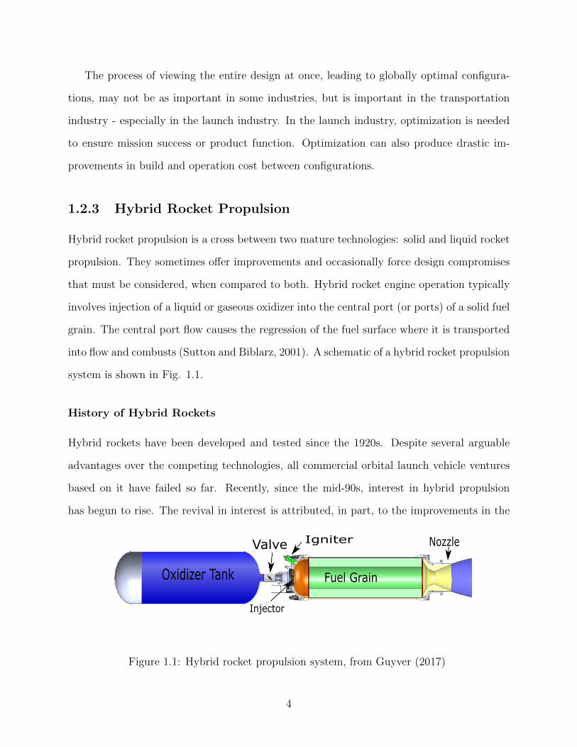
into flow and combusts (Sutton and Biblarz, 2001). A schematic of a hybrid rocket propulsion

system is shown in Fig. 1.1.

History of Hybrid Rockets

Hybrid rockets have been developed and tested since the 1920s. Despite several arguable

advantages over the competing technologies, all commercial orbital launch vehicle ventures

based on it have failed so far. Recently, since the mid-90s, interest in hybrid propulsion

has begun to rise. The revival in interest is attributed, in part, to the improvements in the

Oxidizer Tank Fuel Grain

Injector

Valve Igniter Nozzle

Figure 1.1: Hybrid rocket propulsion system, from Guyver (2017)

4

regression rates of the fuel with the use of liquefying-fuels (Karabeyoglu et al., 2002). The

regression rates are directly tied to mass flow rate and thrust when using a solid fuel grain.

The use of liquefying fuels has made simple single-port configurations more feasible, and

reduced the required surface area of fuel grains by a significant amount.

The history of hybrid rockets begins in the early 1930’s (Altman, 1991; Ribeiro and

Junior, 2011). Initially, American and German researchers tested coal as fuel with nitrous

oxide and gaseous oxygen as candidate oxidizers. Around the same time, Hermann Oberth,

tested tar-wood-saltpeter and liquid oxygen as hybrid rocket propellants. Oberth is known

for early fundamental contributions to rocketry. In 1933 Mikhail Tikhonravov and Sergi

Korolev flight tested a pressure-fed liquid oxygen and gasoline gel HRE (Ribeiro and Junior,

2011). later, in 1956, General Electric tested a high-density-polyethylene and hydrogen

peroxide HRE. In the 1960’s NASA tested a hypergolic HRE with impregnated PBAN, and a

liquid fluorine and oxygen mix as the oxidizer. In 1968 the United States company Beechcraft

developed and tested the Sandpiper target drone which used hybrid rocket propulsion with

PMMA/magnesuim fuel and Mon25 (mixed oxides of nitrogen) oxidizer. In 1983 Teledyne

later developed a more successful target drone, named Firebolt, that entered the United

States Air Force service using PMMA/PB solid fuel and a liquid nitric acid oxidizer. In 1984

the Starstruck Dolphin rocket was tested, which used liquid oxygen / HTPB, with later

testing and development by the American Rocket Company (AMROC). In 1998, the use of

paraffin was reported at Stanford University as a source of performance improvement. The

use of paraffin allowed for a substantial increase in fuel surface regression rate (Karabeyoglu

et al., 2002). Other developments were made by Lockheed in the 2000s and finally Scaled

Composites and SpaceDev developed the nitrous oxide/HTPB hybrid rocket engine for the

sub-orbital vehicle SpaceShipOne whose successor is operating today for Virgin Galactic

as part of its suborbital flight program. Very recently, there has been significant interest

in the application of HREs for launch and in-space propulsion (Schmierer et al., 2019b).

Since the use of HREs can reduce design and mechanical complexity, the technology has

5

the possibility to disrupt the longstanding thinking of the launch and in-space propulsion

industry by potentially offering lower costs of missions. The list of companies, known to this

author, competing in the launch or propulsion industry, using hybrid rocket propulsion is

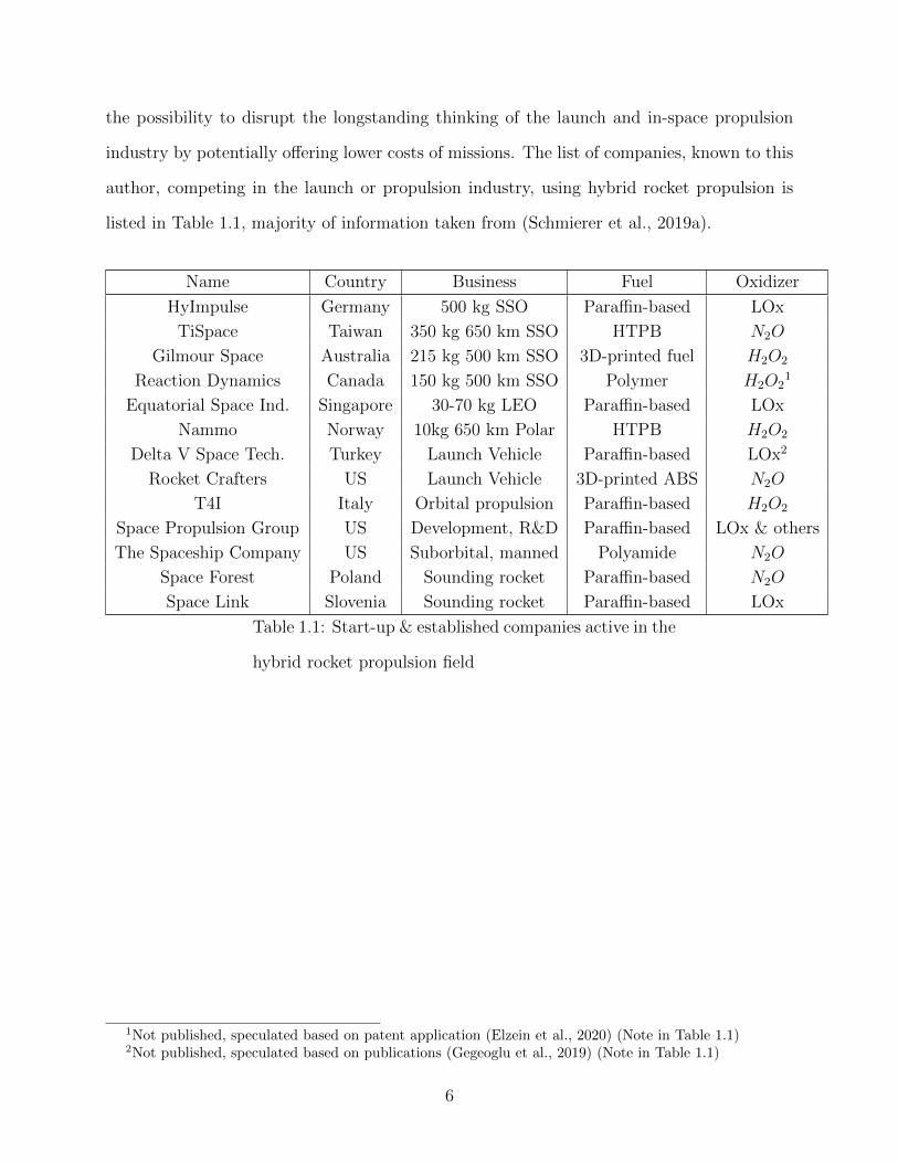
listed in Table 1.1, majority of information taken from (Schmierer et al., 2019a).

Name Country Business Fuel Oxidizer

HyImpulse Germany 500 kg SSO Paraffin-based LOx

TiSpace Taiwan 350 kg 650 km SSO HTPB N2O

Gilmour Space Australia 215 kg 500 km SSO 3D-printed fuel H2O2

Reaction Dynamics Canada 150 kg 500 km SSO Polymer H2O21

Equatorial Space Ind. Singapore 30-70 kg LEO Paraffin-based LOx

Nammo Norway 10kg 650 km Polar HTPB H2O2

Delta V Space Tech. Turkey Launch Vehicle Paraffin-based LOx2

Rocket Crafters US Launch Vehicle 3D-printed ABS N2O

T4I Italy Orbital propulsion Paraffin-based H2O2

Space Propulsion Group US Development, R&D Paraffin-based LOx & others

The Spaceship Company US Suborbital, manned Polyamide N2O

Space Forest Poland Sounding rocket Paraffin-based N2O

Space Link Slovenia Sounding rocket Paraffin-based LOx

Table 1.1: Start-up & established companies active in the

hybrid rocket propulsion field

1Not published, speculated based on patent application (Elzein et al., 2020) (Note in Table 1.1)2Not published, speculated based on publications (Gegeoglu et al., 2019) (Note in Table 1.1)

6

Some of the advantages and disadvantages of hybrid rocket propulsion are organized

below:

Advantages

� An intimate mixture of fuel and oxidizer cannot be easily made if the single oxidizer

tank was to catastrophically fail. This safer failure mechanism greatly reduces the

explosion potential compared to liquid rocket engines (LREs).

� The solid fuel grains are inert at ambient conditions in the absence of an oxidizer,

making them safer to manufacture and transport compared to solid propellant rocket

motors (SRMs).

� Grain failure (e.g., sloughing) in a hybrid is benign compared to SRMs. In SRMs, grain

failure leads to increased burn rate and over-pressurization and catastrophic failure,

since burn rate is pressure-dependent (Sutton and Biblarz, 2001).

� HREs can be throttled and terminated mid-burn with the use of a single valve, unlike

SRMs.

� Energetic or stability-promoting additives can more easily be introduced to the propel-

lants, compared to LREs. For example, additives like metal particles can be suspended

in the solid fuel grain.

� The system complexity can be reduced relative to existing LREs since only the control

and injection of one fluid propellant is required.

� The density of fuel is increased, compared to liquid fuels, since it exists in the solid

phase.

� The combustion chamber doubles as a “fuel tank”. This point can be viewed as either

an advantage or disadvantage, depending on the type of feed system (if propellant

7

storage pressure is above or below combustion chamber pressure).

Disadvantages

� Typically liquid fuels are used in regenerative cooling applications in LREs. The fuels

are typically chosen over the oxidizers to avoid oxidation issues. Regenerative cooling

cannot be as readily done with a liquid oxidizer in the case of a HRE.

� In HREs, in addition to the chosen oxidizer mass injection rate setting, the effective

oxidizer-to-fuel ratio OF is a function of two other things: fuel burning surface area

and the local axial mass flux G (which drives the fuel surface regression rate, in a con-

ventional HRE). These two quantities, in general, increase and decrease concurrently

during a burn. Generally, their effects are not equal and the oxidizer-to-fuel ratio shifts

during a nominal burn (Kuo and Chiaverini, 2007).

� Gimbaling of the entire engine is difficult/impractical compared to relatively small-

chambered LREs.

� The HRE technology as a whole is less mature since its use is infrequent, compared to

existing technologies (Kuo and Chiaverini, 2007).

Feed systems

Two main feed systems are considered in this thesis: electric pump-fed and pressure-fed. The

pressure-fed category is comprised of self-pressurizing and back-fill pressurant-based systems.

The self-pressurizing systems rely on two-phase fluids with a relatively high vapour pressure

and liquid density at standard conditions (Zimmerman et al., 2013). Self-pressurizing pro-

pellants (in this case, oxidizers) maintain pressure upon depletion of liquid oxidizer from

the system. Back-fill, or gas pressure-fed systems, use a pressurizing system comprised of

a separate high-pressure storage vessel and a regulator (Sutton and Biblarz, 2001). When

compared to pump-fed variants, the pressure-fed systems are inherently simpler. Pressure-

8

fed systems typically have larger inert masses since the tank pressure must be sufficiently

higher than the combustion chamber pressure, while pump-fed systems (with pressurization

downstream of storage) can have relatively low-pressure storage tanks (Sutton and Biblarz,

2001).

Pump-fed systems have typically used turbine-driven pumps, called turbopumps. In tur-

bopump feed systems, the pump is driven by a turbine fed with a working fluid. Electric

pump feed systems have a battery-powered electric motor in place of the classical turbine.

The electric pump feed system has been considered since the 1990’s for liquid bi-propellant

systems and have shown to be as a higher-performing alternative to back-fill pressure-fed

configurations for hybrid systems (Casalino et al., 2019b). Advances in battery technolo-

gies have made this feed system increasingly competitive (Rachov et al., 2013). Recently,

Rocket Lab’s Electron launch vehicle completed its 14th flight using Rutherford LREs with

an electrically-driven pump feed system (RocketLab, 2020a).

1.3 Research Objectives

One of the research goals of this thesis is to answer the question: to what extent can hybrid

rocket launch vehicles be scaled down? Put differently, and generally - what is the minimal

size (gross liftoff mass or dry mass) of a two-stage hybrid rocket launch vehicle for a given

payload mass, delivered to a low Earth orbit (LEO)? The minimization of dry mass is in

general desirable, as the dry mass is assumed to be strongly linked to cost, in dollars. The

use of dry mass in the absence of detailed cost data is a commonly used strategy by other

researchers (Castellini, 2012; Miranda, 2015).

A follow up research question question is what does the minimal (optimal) configuration

look like for different vehicle configurations (feed systems and propellant types)? The goals

of this thesis are to answer these research questions, along with creating the framework

necessary to attempt to answer them. The framework will be a combination of mathematical

9

models, simulating the physics of the various disciplines relevant to the performance of

a hybrid rocket launch vehicle. The models will be incorporated into an object-oriented

computer program, written in Python.

1.4 Methodology

The design space of a hybrid rocket vehicle is divided into the various relevant sub-disciplines.

The design variables, for this study, were desired to be limited to the most fundamental

defining physical quantities possible. The design variables, seen as inputs or constants,

dictate the design of the launch vehicle as it propagates through the various sub-disciplines.

The propulsion system is the first conceptually designed sub-system. Orbital launch ve-

hicles are typically comprised of a large portion of propellant, on a mass basis, which is

necessary to fulfill the mission requirements (Larson and Wetrz, 1999). The propulsion sys-

tem designed dictates: the propellant masses, propellant volumes, propulsive performance,

and fuel and converging-diverging nozzle geometries. The vehicle structural configurations

are then defined by vehicle elements (oxidizer tank, interstage, etc.), in order to close the

design further. Structural and geometric inputs and constants (outer diameter, nosecone,

etc.) further constrain the design. The aerodynamic modeling provides the aerodynamic

forces, given the vehicle geometry and the simulated environment, resulting in the ability

to calculate the vehicle dynamics and loads. The structure is then iteratively sized, based

on material yield stress and buckling failure modes using in-flight and on-pad structural

loads. The trajectory is converged to the target altitude and speed by altering initial flight

path conditions and trajectory control points, while minimizing overall propellant use. The

described process results in a single vehicle design solution. Numerous vehicle designs are

then evaluated and successive design iterations altered using global optimization techniques

dedicated to minimizing dry mass. The minimization of dry mass, for a given mission, results

in optimal designs and the corresponding design variables.

10

Chapter 2

Literature Review

The following literature review surveys work on launch vehicle MDO. Within launch vehicle

MDO, the engineering models and the MDO implementation strategies were assessed. Most

works have been on large-scale liquid bi-propellant and SRM-based launchers. A relevant

work on small-satellite hybrid launchers was found and reviewed. Work on small-satellite

launch vehicle design, based on SRM and liquid bi-propellant technology, was investigated.

Finally, there were several works found on hybrid rocket conceptual design that mainly

focused on the optimization of the propulsion system quantities but avoided other disciplines.

2.1 Launch Vehicle MDO

The MDO of launch vehicles has been a topic of research for several years. The majority of

studies investigated here focus on liquid bi-propellant and solid rocket-propelled expendable

launchers. The studies surveyed on launch vehicle MDO have been decomposed into the

MDO formulation and the engineering models. The engineering models are naturally divided

into their respective disciplines (propulsion, aerodynamics, etc.).

11

2.1.1 Liquid Bi-propellant and Solid Rocket MDO

The work of Bayley (2007) was one of the earliest works on launch vehicle MDO. Bayley

included the use of a genetic algorithm (GA) to optimize Earth-to-orbit SRM and LRE-

based multi-stage rockets. The objective of the work was to minimize gross-take-off weight

for a given mission. The propulsion modeling consisted of non-time-varying parameters:

chamber pressure, and characteristic velocity, but incorporated varying thrust with changing

back pressure. The structural elements were defined with user inputs rather than physics-

based or even historical-based empirical methods. A closed-source missile aerodynamics

design software was used to query aerodynamic coefficients for use with a six degree of

freedom (6DOF) flight dynamics simulation. Despite that lack of physics-based formulation

for the structural design, the validation study seemed to show agreement with existing rocket

designs. The results showed that increasing scale increased a vehicle’s payload mass fraction.

In contrast to maximizing payload fraction (or minimizing mass for a given payload),

research was done towards estimating the cost and reliability of launch vehicles during the

conceptual design phase (Krevor, 2007). Krevor’s work included an optimization (maxi-

mizing reliability with minimal cost) using a GA. The vehicle mass was estimated using

historical data from previous launch vehicle designs, which exist as empirical relations, com-

monly used and refereed to as mass estimating relationships (MERs). The propulsion system

parameters were estimated using a tool called the Rocket Engine Design Tool for Optimal

Performance - 2 (REDTOP-2) (Bradford et al., 2004). The REDTOP-2 tool returned thrust-

to-weight ratios of the engine and specific impulse, given the defining input parameters: fuel

type, oxidizer type, chamber pressure, and expansion ratio. The trajectory analysis in this

methodology was completed using the Program to Optimize Simulated Trajectories (POST)

(Brauer, 1975), which is a 3DOF trajectory simulation widely used at NASA. The work’s

contribution was mainly in the area of predicting and maximizing reliability while minimizing

cost, and used existing modules to carry out the vehicle design aspect.

12

Engineering Model Advancements

The engineering discipline modeling fidelity used in launch vehicle MDO was greatly im-

proved by the work of Castellini (Castellini, 2012; Castellini et al., 2014). Castellini’s PhD

dissertation described a MDO with a focus on the engineering formulation of launch ve-

hicle conceptual design. The thesis reviewed many pieces of work, to its date, on MDO

for aerospace vehicle design. The review of MDO presents the classifications advanced by

Cramer et al. (1992). The work by Cramer et al. (1992) includes the Multi-disciplinary

Feasible (MDF) and Individual Disciplines Feasible (IDF) formulations. A MDF framework

is the most intuitive since the design is, at all iterations, feasible, such as moving a design

from inputs through various departments (disciplines) to output. However, MDF, at some

times, can waste computational resources on ensuring a feasible design during each itera-

tion. The IDF framework introduces feasibility constraints at each interdisciplinary stage

but the global optimizer drives the individual disciplines towards feasibility only at the end

of the optimization process. IDF adds a constraint and parameter per interdisciplinary cou-

pling, but in some situations can reduce the number of total design iterations. An analysis

conducted by Castellini shows that MDF proved superior to IDF in launch vehicle design.

Castellini had short iteration times but if loop time was increased, maybe with the use of

high-computation-cost CFD or FEM, the extra effort in formulating the IDF framework

could have proved worthwhile. Castellini presented the use of particle swarm optimization

(PSO) and GA as the most promising global optimization schemes for launch vehicle design,

suggesting the superiority of PSO’s performance given the evidence in literature. Castellini

found that PSO outperformed the GA in terms of convergence rate and consistency of finding

the global optimal, and used it to generate all results.

The launch vehicle conceptual design models, which were the main focus of Castellini’s

work, were divided into two sections named conceptual and early-preliminary. The early-

preliminary section was the result of feedback from an initial validation study and meetings

with the European Space Agency’s (ESA)’s engineers and specialists about the initial con-

13

ceptual framework. The overall vehicle structures included serial and or parallel staging

of LRE and or SRM rocket boosters. The propulsion system design could either be de-

fined based on existing engines (off-the-shelf database), or on fundamental SRM or LRE

propulsion theory. The performance of new designs, of a chosen propellant combination,

was predicted using NASA Chemical Equilibrium with Applications (CEA) (Sanford and

Mcbride, 1994) for given mixture ratios and combustion pressure. The CEA outputs were

used, assuming isentropic expansion, to determine theoretical specific impulse and nozzle ge-

ometry. Detailed combustion and nozzle efficiencies were applied based on combustion and

nozzle design parameters. It was noted that certain efficiencies must be introduced to gener-

ate performance values that resemble operational engine’s data, as the vehicle performance

(payload mass for a mission) had the highest sensitivity to the propulsive performance. The

nozzle and combustion efficiencies account for the divergence angle of the nozzle exit flow,

boundary layer losses, finite combustion area, and real gas properties. All non-structural

mass components were determined from MERs. The structural components were sized using

structural material stress-based methods outlined for combined axial, bending, and pres-

sure loads with thin-cylinder buckling for compression. Missile Datcom (Blake, 1998) was

used for the aerodynamic parameters for the ogive-cylinder geometry used. The conceptual

framework allowed diameter changes as well as side boosters, the latter of which could not

be handled by Datcom. A simple averaging scheme was proposed and used for the additional

drag and normal force from side boosters, which was used with a single validation point and

with the admittance of probable inaccuracy. The choice of the aerodynamic modeling was

defended by showing low sensitivity of the vehicle performance (payload mass for a mission)

to uncertainty in drag. The flight simulation was modeled assuming a point mass in a 6DOF

spherical-Earth coordinate system. The trajectory consisted of a pitch over after launch into

an optimizible gravity turn, bi-linear tangent steering program, and upper stage coast and

circularization burn. Castellini included cost, reliability and safety into the conceptual study

by using cost estimating relationships and component failure probabilities based on histor-

14

ical data. After two successive validation runs comparing the code to the Ariane 5 ECA

and VEGA launchers, Castellini concluded that predicted inert mass error was the largest

contributor to the variance in deliverable payload mass (5%). The predicted error in propul-

sion system performance lead to a 3% difference in payload mass, and aerodynamic drag

and normal force error lead to 2% difference in payload mass. The final, revised, conceptual

methodology: called early preliminary was concluded to predict payload masses within 4 %

and 6% for the Ariane 5 ECA and VEGA launchers, concluding that it is possible to develop

relatively simple models permitting fast MDO cycles while still ensuring sufficient accuracy

to place confidence in the achieved design solutions for expendable launch vehicles.

Mota (2015) used many of the engineering models used by Castellini. Mota’s main

contribution was in introducing a novel formulation to optimize trajectories by mixing a

direct method and indirect method. The direct method used typical control point adjustment

while drag effects were present in the atmosphere. Outside of the atmosphere, where drag

could be neglected, the initial co-state variables for optimal thrust arcs in vacuum could were

calculated in the indirect method. The method supplies optimal thrust arcs for the upper

stages but still requires converging to the desired orbit and optimization using a non-linear

algorithm.

The expendable launch vehicle MDO knowledge base was expanded by introducing first

stage re-use modeling (Woodward, 2017). Woodward developed a tool for expendable and

first-stage-boost-back reusable launch vehicle conceptual design. The work started with a

comprehensive review on the state of the art of conceptual design and optimization of launch

vehicles from both commercial and academic sources. In the conceptual design methodology,

the propulsion system was characterized by constant specific impulse. MERs were used for

the entire vehicle design, with no stress-based sizing. The trajectory was optimized using

pitch rate parameters defined at instants into the burn as optimization variables coupled

with a gravity turn and maximum dynamic pressure constraints. The flight simulation was

conducted using a 3DOF round-Earth formulation which simulated initial flight and boost-

15

back. The aerodynamic coefficients were determined using missile aerodynamic empirical

relations from Fleeman (2012). Woodward chose to keep track of the performance parameter

∆V , calculated using the Tsiolkovsky rocket equation (Moore, 1813) from specific impulse

and mass fractions of the vehicles. The ∆V is the change in velocity of a launch vehicle and

is a a measure of impulse per unit mass needed to perform a maneuver including launching

to orbit. The net required ∆V budget was calculated incorporating drag, gravity, and

steering losses which were quantified from the flight simulation. Their study was validated

by comparing to existing rockets, which included: Gemini Launch vehicle (Titan II), Saturn

V, and Falcon 9. It was estimated that the delta V losses that were predicted had an error

on the order of 10%.

MDO Implementation

The MDO formulation, instead of the engineering modeling, was the main focus of other

work (Balesdent, 2011). Balesdent wrote a very comprehensive and formal mathematical

definition and review of MDO theory. Balesdent suggested that putting trajectory at the

center of the optimization and having stage-wise optimization with defined coupling parame-

ters would yield global optimal results efficiently. The entire problem was formulated as IDF

and coupling parameters were defined between structures, propulsion, aerodynamics, and

trajectory. The propulsion system modeling of Balesdent’s work was a constant property

system with constant chamber pressure and mass flow rates but altitude (back pressure)

compensated. The aerodynamic drag was considered solely a function of Mach number, ap-

pearing un-cited. The trajectory was modeled as a piece-wise linear function of pitch angle

vs time into flight, with optimization control points. A three-degree-of-freedom non-rotating

spherical-Earth formulation was used for the flight simulation. The mass estimates for all

vehicle structures and components were accomplished using MERs. The pressure vessel mass

sizing was stress-based. The work appears to be very detailed in the MOD review and IDF

formulation, however it does not contribute greatly to the launch vehicle design knowledge

16

base in the conceptual design of launch vehicles, and calls upon very basic functions.

2.1.2 Hybrid Rocket MDO

Miranda (2015), was found to be the only researcher who presented a comprehensive MDO for

hybrid launch vehicles. Miranda conducted conceptual optimization studies on air-launched

and ground-launched hybrid rockets. The optimization objective function included vehicle

gross-take-off mass. Miranda’s research question was: how do hybrid rocket vehicles (both

ground and air-launched) compare to existing SRM technology in terms of cost and perfor-

mance? Miranda, in short, found they had similar performance. Hybrid rocket vehicles had

lower propellant mass fractions but higher specific impulse, compared to SRMs. Miranda

built off the work of Van Kesteren (2013) on solid rocket conceptual design. Miranda’s

methodology included hybrid empirical regression rate law and used NASA CEA to pre-

dict combustion properties. The combustion products were expanded assuming frozen flow

through the nozzle and isentropic relations. The formulation did not account for any time-

varying aspects of hybrid propulsion such as the oxidizer-to-fuel ratio (OF ) shift, however its

absence was acknowledged and mentioned in the future work section. Oxidizer and combus-

tion chamber tanks and cylindrical sections were sized using stress-based methods from axial

and bending loads in-flight, while all other components used MERs. Missile Datcom was

used for the aerodynamic coefficients. A 3DOF round-Earth model was used for simulating

trajectories to orbit. The global optimization techniques used were GA and PSO. Miranda

found that PSO out-performed the GA used. Miranda concluded the model was valid when

comparing to data available from the NAMMO hybrid rocket (Faenza et al., 2019). The

data of the NAMMO launcher was however redacted from the thesis. The work also showed

that the vehicle can weigh substantially less (up to 75%) when air launching is used. The

work found the minimized gross-take-off mass for a ground-launched 10 kg to 780 km circular

LEO three-stage sorbitol/N2O hybrid launch vehicle to be 1710 kg. The work concluded that

hybrid rocket vehicles can have equal or greater performance than solid-rocket-based propul-

17

sion, since HREs offer theoretical higher performance but currently have lower propellant

mass fractions. Future work suggestions also included adding OF and throttling parameters

as optimization variables and using faster computing code with parallel computing for opti-

mization studies. Miranda also suggested incorporating fluid equations of states and higher

fidelity propulsion modules for further detailed preliminary design studies and optimization.

The work of Miranda shares many similarities in modeling methodology with the work

in this thesis. Miranda’s thesis also produced designs. Much of the suggested future work by

Miranda was addressed in this work. The recommendations of Miranda and the suggested

work are combined in the following:

� Implement the constraints of the solution-space directly into the optimizer.

� Use parallel computing and computational resources greater than a common desktop.

� Conduct a more extensive review of existing hybrid rocket technology.

� Explore more fuel and oxidizer combinations.

� Explore different oxidizer storage conditions.

� Include propellant oxidizer-to-fuel ratio and oxidizer flow rate as optimization variables.

� Prioritize fast computation in all code.

On top of the suggestions by Miranda, there were also many changes and refinement to

the modeling methodology that took place that resulted in different findings of optimal and

feasible configurations.

2.2 Hybrid Rocket Propulsion Design and Optimiza-

tion

Initial hybrid rocket conceptual design was accomplished by analyzing the replacement of

LRE and SRM upper-stages with hybrid alternatives. Casalino and Pastrone (2010a) inves-

tigated the optimization of a hybrid rocket upper stage to replace a SRM and LRE 3rd and

4th stage. The trajectory and motor parameters of a polyethylene and hydrogen peroxide

motor were considered in a conceptual design optimization. Optimization parameters for

18

the motor included: number of ports, fuel geometry, initial thrust, chamber pressure, length,

and nozzle area ratio. The ideal OF was found to differ from that corresponding to the

highest specific impulse. It was found that a single pressure-fed hybrid stage could replace

the third and fourth SRM and LRE stages for a four stage rocket with a mission profile based

on the Vega launcher. Karabeyoglu et al. (2011) expanded the hybrid propulsion conceptual

design literature by analyzing a pressure-fed hybrid for the replacement of an existing upper

stage. The investigated propulsion systems were based on paraffin and liquid oxygen and

were compared to existing all-SRM and all-LRE technologies. A single-port fuel configura-

tion was used with hoop stress and Mach number constraints on the initial port diameter.

Karabeyoglu et al. (2011) found that a pressure-fed upper stage had an advantage over a

SRM upper stage due to its higher specific impulse. A 25% increase in payload mass was

possible when using neat paraffin with liquid oxygen over the Orion 38 solid rocket motor

upper stage. It was also found up to 40% payload increase was theoretically possible when

using high-density performance additives. Karabeyoglu et al. concluded with a list of key

technology developments needed for the advancement of HREs:

� Retaining high efficiencies and good stability for long duration burns

� Controlling/limiting the nozzle erosion rates

� Nozzle development

� Vacuum ignition and multiple ignitions

� Throttling

� Thrust augmentation for control: LITVC or GITVC capability

Casalino and Pastrone (2010b) added to their previous work by incorporating an electric

pump feed system to HREs that would improve payload capability over the pressure-fed

configuration. After the uptake of the electric pump feed cycle, Casalino et al. (2019b) wrote

on the viability of using electric pump feed systems and produced more detailed quantitative

analysis compared to his previous publications. In the recent work of Casalino et al. (2019b),

three different feed systems were considered for a paraffin/ liquid oxygen hybrid rocket upper

stage for a Vega-like launcher. The three propulsion systems were gas pressure-fed, electric

19

pump-fed, and advanced electric pump-fed. The trajectory error was minimized and payload

mass concurrently maximized using a PSO. Six optimization parameters were used to define

the design, the first five were: the grain outer radius, the web thickness, the fuel grain length,

the final exhausted oxidizer mass, and the initial nozzle area ratio. The sixth parameter was

the exhausted oxidizer mass for pressure-fed or pump discharge pressure for the pump-fed

case. The increased payload mass over the pressure-fed case was found to be 12% and 18%

for the electric pump and advanced electric pump versions respectively.

Casalino et al. (2019a) recently contributed to the area of small-satellite hybrid launcher

conceptual design with a design and optimization of a three-stage pressure-fed hybrid small-

satellite launcher. The launcher was based on a paraffin/liquid oxygen engine. The number of

engines in each stage were six, three, and one for the stages, from first to last, respectively.

The gross takeoff mass was set at 5000 kg while the payload mass was maximized. The

optimization variables included: fuel grain outer radius, OF , pressurant gas volume, and

overall oxidizer mass exhausted. The trajectory was optimized in an inner-loop for each

motor configuration. The five motor parameters were simultaneously converged to their

optimal values using a PSO to maximize payload mass. The design robustness was evaluated

by incorporation deviations in the motor parameters (regression constants). The conservative

estimate where each engine operated at the worst off-nominal conditions resulted in a 15 kg,

or 26% payload reduction.

2.3 Small Launch Vehicle Design

Articles on the topic of small-payload orbital launch vehicles were reviewed. Whitehead

(2005) asked the question: how small can a launch vehicle be? The author analyzed the

ascent trajectory and drag effects on SRM and LRE-based rockets at different scales. White-

head found that the effect of drag on smaller launch vehicles was relatively larger and resulted

in higher required ∆V to attain the same orbit. The higher influence of drag on performance

20

was mitigated by steeper simulated launch trajectories, where the rocket spends less time in

the atmosphere, but this also comes at a cost of higher ∆V due to larger circulation burns.

It was concluded that scaling down does not impose a physical limit on launch vehicle size

from the ascent and trajectory standpoint but increases required ∆V slightly. Whitehead

states the technological challenge is obtaining high propellant mass fractions on such small

launch vehicles, namely when components must be impractically small.

Greatrix and Karpynczyk (2005) presented a more detailed vehicle design concept for a

relatively low-cost small-payload delivery to orbit. They presented two designs of a three-

stage solid rocket configuration, one for air-launch and one for ground-launch. The payload

was in the nano-satellite range of 10 kg. The target orbit was approximately 320 km orbit

launching eastward in the proximity of Churchill Manitoba. A significant coast was used

between 2nd stage burnout and 3rd stage re-light in order to coast to target altitude before

conducting a ciruculization burn. The trajectories incorporated a steep ascent until outside

of the atmosphere followed by aggressive turning accomplished by side thrusters. The motion

was modeled using a 6DOF round earth formulation with aerodynamics from Missile Datcom.

The reduced drag and ∆V requirements from air launching resulted in a vehicle gross mass

of 1900 kg, versus 4500 kg for the ground launch case. The concluding remarks suggest

addressed the use of HREs for low cost access to space citing the high specific impulse and

availability of propellants compared to SRMs.

2.4 Summary and Areas of Improvement

The literature relating to launch vehicle MDO has mainly been comprised of large-scale liquid

bi-propellant and SRM expendable launchers optimized based on paylaod fraction. Building

on payload fraction optimizations, cost and reliability have been modeled and implemented

into the MDO process. Later researchers worked to review, refine, and add fidelity to the

engineering models to generate detailed results. Parallel to the engineering model refinement,

21

some researchers focused on the MDO process and proposed and used different strategies

with less contributions to the engineering models. Recent work incorporated re-usability into

the launch vehicle conceptual design process. MDO has been shown to be a powerful tool is

producing high-performing launch vehicles. However, many of the empirical mass estimating

relations used for large-scale vehicles are not effective for small-scale vehicle design. As such,

there have been many recent works devoted to conceptual design at the smaller scale. Given

the reviewed literature, the smallest conceptual launchers investigated have been in the range

of 10 kg payload capability. The only identified drawbacks of very small launchers have been

an increased influence of drag and impracticality of miniature hardware. Much of the work

on hybrid rocket conceptual design and optimization has focused on the propulsion system

specifically, without significant detail given to other disciplines.

Contributions can be made by expanding the current hybrid rocket full-vehicle MDO

knowledge, especially with the recent propulsion system modeling using paraffin fuel and

the electric pump feed system. The identified area of improvement in hybrid rocket launch

vehicle MDO literature, coupled with the recent increase in small-satellite launcher design

and development, offer the motivation for the present work. The present conceptual design

framework will aim to use physics-based modeling given the lack of historical data and

empirical mass models for small launchers.

22

Chapter 3

Mathematical Modeling

The change in velocity (∆V ) of a launch vehicle or spacecraft is a measure of the impulse

per unit mass needed to perform a maneuver such as launching to orbit or an in-space

orbital maneuver (Vallado, 2010). The ∆V of a launch vehicle can be determined using the

Tsiolkovsky rocket equation:

∆V = velnm0

mf

= Ispg0lnm0

mf

(3.1)

Where ve is the nozzle exit velocity, Isp is the specific impulse , and g0 is Earth’s standard

gravitational acceleration. The values m0 and mf are the vehicle initial and final masses

respectively. The derivation of the rocket equation can be first found by Moore (1813). The

equation is derived by applying conservation of momentum on a one-dimensional vehicle

with aligned thrust and velocity vectors. The derivation assumes an impulsive thrust and

constant exhaust velocity. The derivation of the rocket equation neglects aerodynamic drag

and gravity, and more subtly neglects steering losses, which arise whenever the direction of

the thrust vector differs from that of the vehicle’s forward velocity vector. Under the array

of assumptions, mentioned above, the ∆V is remarkably only dependent on the propulsive

performance (specific impulse , Isp) and structural efficiency (mass ratio, m0

mf). It is evident

from this relation that one should strive to minimize inert (dry) mass of a launch vehicle

23

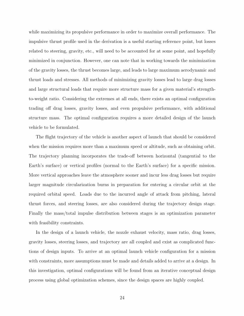
while maximizing its propulsive performance in order to maximize overall performance. The

impulsive thrust profile used in the derivation is a useful starting reference point, but losses

related to steering, gravity, etc., will need to be accounted for at some point, and hopefully

minimized in conjunction. However, one can note that in working towards the minimization

of the gravity losses, the thrust becomes large, and leads to large maximum aerodynamic and

thrust loads and stresses. All methods of minimizing gravity losses lead to large drag losses

and large structural loads that require more structure mass for a given material’s strength-

to-weight ratio. Considering the extremes at all ends, there exists an optimal configuration

trading off drag losses, gravity losses, and even propulsive performance, with additional

structure mass. The optimal configuration requires a more detailed design of the launch

vehicle to be formulated.

The flight trajectory of the vehicle is another aspect of launch that should be considered

when the mission requires more than a maximum speed or altitude, such as obtaining orbit.

The trajectory planning incorporates the trade-off between horizontal (tangential to the

Earth’s surface) or vertical profiles (normal to the Earth’s surface) for a specific mission.

More vertical approaches leave the atmosphere sooner and incur less drag losses but require

larger magnitude circularization burns in preparation for entering a circular orbit at the

required orbital speed. Loads due to the incurred angle of attack from pitching, lateral

thrust forces, and steering losses, are also considered during the trajectory design stage.

Finally the mass/total impulse distribution between stages is an optimization parameter

with feasibility constraints.

In the design of a launch vehicle, the nozzle exhaust velocity, mass ratio, drag losses,

gravity losses, steering losses, and trajectory are all coupled and exist as complicated func-

tions of design inputs. To arrive at an optimal launch vehicle configuration for a mission

with constraints, more assumptions must be made and details added to arrive at a design. In

this investigation, optimal configurations will be found from an iterative conceptual design

process using global optimization schemes, since the design spaces are highly coupled.

24

During the modeling formulation, inputs are selected that define physical quantities. Any

parameter that is referred to in this methodology section may be seen as a constant or an

optimization variable; the distinction will be made later.

3.1 Propulsion System Modeling

In this section, the propellant masses, solid grain fuel geometry, nozzle geometry, and com-

ponent masses associated with a given feed system and propellant configuration are defined.

3.1.1 Initial Scaling Parameters and Propellant Attributes

The initial parameters specified are the rocket engine(s) nominal average thrust, Tav, and

total impulse, It. The burn time, tb, can be equivalently used to replace either the thrust or

total impulse parameters. The burn time is simply related to the other initial quantities by

Eqn. 3.2:

tb =ItTav

(3.2)

Since the total impulse and thrust are dependent on back pressure (outside ambient air

pressure, which decreases with increasing altitude) for fixed geometry nozzles, the parame-

ters are more accurately defined as liftoff thrust and sea-level total impulse. The sea-level

definitions are generalized, with staging in mind, for any altitude, and are defined as thrust

and total impulse - at ignition conditions.

The propellant combinations used in this thesis include paraffin wax with either liquid

oxygen (LOx) or nitrous oxide (N2O). The commonly used, axial-length-averaged fuel surface

regression parameters of the fuel/oxidizer combinations investigated here, were found in

literature (Karabeyoglu et al., 2007; Paccagnella et al., 2019). The relevant regression rate

coefficients are presented in Table 3.1. The a parameters are for regression rates in m/s rates

for flux values with units of kgm2s

.

25

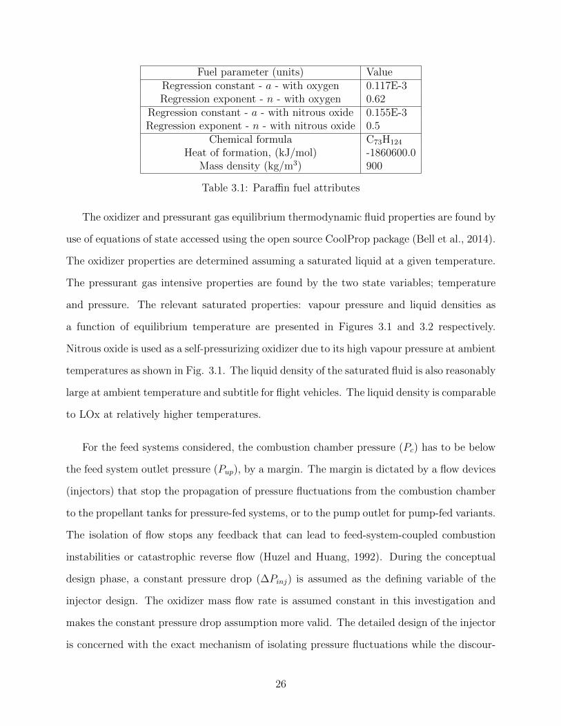
Fuel parameter (units) ValueRegression constant - a - with oxygen 0.117E-3Regression exponent - n - with oxygen 0.62

Regression constant - a - with nitrous oxide 0.155E-3Regression exponent - n - with nitrous oxide 0.5

Chemical formula C73H124

Heat of formation, (kJ/mol) -1860600.0Mass density (kg/m3) 900

Table 3.1: Paraffin fuel attributes

The oxidizer and pressurant gas equilibrium thermodynamic fluid properties are found by

use of equations of state accessed using the open source CoolProp package (Bell et al., 2014).

The oxidizer properties are determined assuming a saturated liquid at a given temperature.

The pressurant gas intensive properties are found by the two state variables; temperature

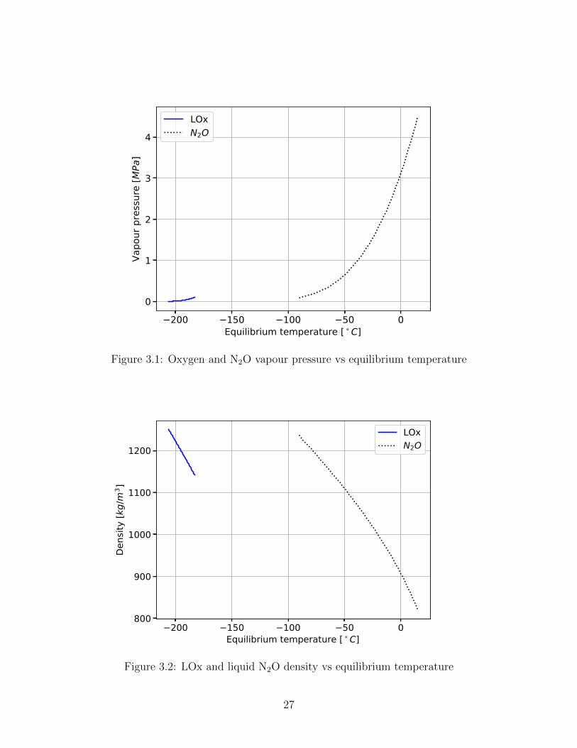
and pressure. The relevant saturated properties: vapour pressure and liquid densities as

a function of equilibrium temperature are presented in Figures 3.1 and 3.2 respectively.

Nitrous oxide is used as a self-pressurizing oxidizer due to its high vapour pressure at ambient

temperatures as shown in Fig. 3.1. The liquid density of the saturated fluid is also reasonably

large at ambient temperature and subtitle for flight vehicles. The liquid density is comparable

to LOx at relatively higher temperatures.

For the feed systems considered, the combustion chamber pressure (Pc) has to be below

the feed system outlet pressure (Pup), by a margin. The margin is dictated by a flow devices

(injectors) that stop the propagation of pressure fluctuations from the combustion chamber

to the propellant tanks for pressure-fed systems, or to the pump outlet for pump-fed variants.

The isolation of flow stops any feedback that can lead to feed-system-coupled combustion

instabilities or catastrophic reverse flow (Huzel and Huang, 1992). During the conceptual

design phase, a constant pressure drop (∆Pinj) is assumed as the defining variable of the

injector design. The oxidizer mass flow rate is assumed constant in this investigation and

makes the constant pressure drop assumption more valid. The detailed design of the injector

is concerned with the exact mechanism of isolating pressure fluctuations while the discour-

26

200 150 100 50 0Equilibrium temperature [ C]

0

1

2

3

4Va

pour

pre

ssur

e [M

Pa]

LOxN2O

Figure 3.1: Oxygen and N2O vapour pressure vs equilibrium temperature

200 150 100 50 0Equilibrium temperature [ C]

800

900

1000

1100

1200

Dens

ity [k

g/m

3 ]

LOxN2O

Figure 3.2: LOx and liquid N2O density vs equilibrium temperature

27

aging of backflow, while, from the system point of view, must minimize pressure drop for a

given flow rate. The injector must also promote effective spray, atomization, mixing, and

stability for the combustion reaction.

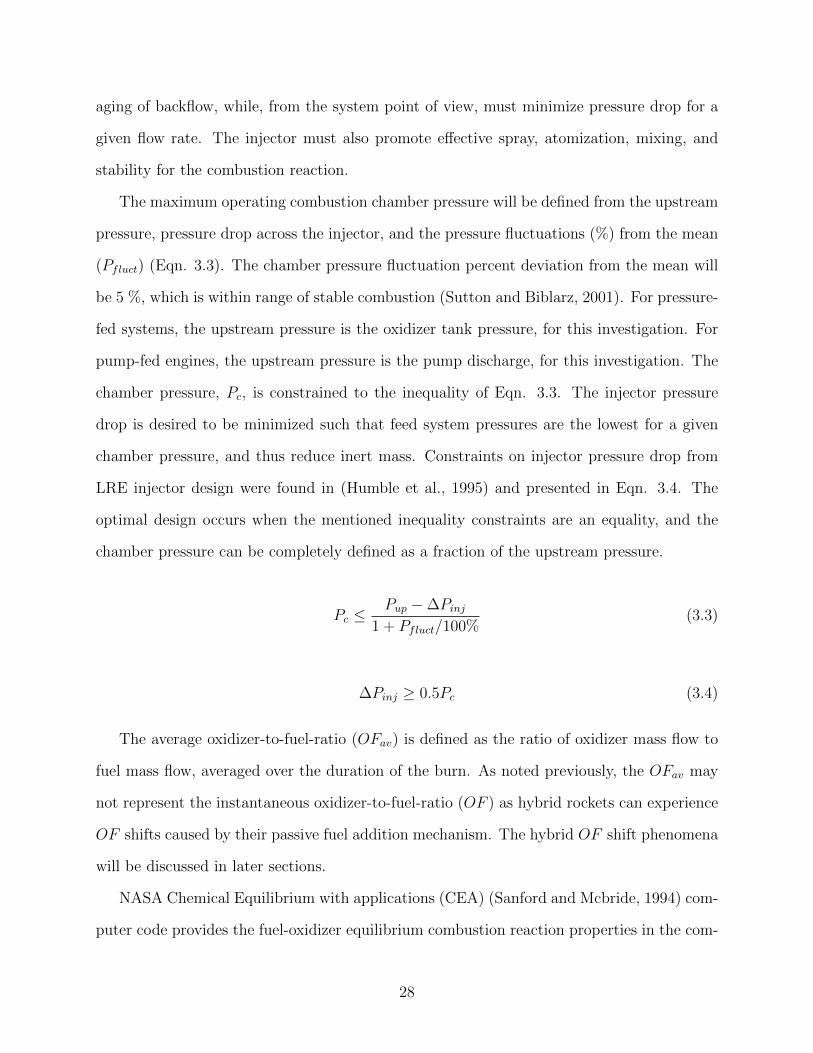
The maximum operating combustion chamber pressure will be defined from the upstream

pressure, pressure drop across the injector, and the pressure fluctuations (%) from the mean

(Pfluct) (Eqn. 3.3). The chamber pressure fluctuation percent deviation from the mean will

be 5 %, which is within range of stable combustion (Sutton and Biblarz, 2001). For pressure-

fed systems, the upstream pressure is the oxidizer tank pressure, for this investigation. For

pump-fed engines, the upstream pressure is the pump discharge, for this investigation. The

chamber pressure, Pc, is constrained to the inequality of Eqn. 3.3. The injector pressure

drop is desired to be minimized such that feed system pressures are the lowest for a given

chamber pressure, and thus reduce inert mass. Constraints on injector pressure drop from

LRE injector design were found in (Humble et al., 1995) and presented in Eqn. 3.4. The

optimal design occurs when the mentioned inequality constraints are an equality, and the

chamber pressure can be completely defined as a fraction of the upstream pressure.

Pc ≤Pup −∆Pinj

1 + Pfluct/100%(3.3)

∆Pinj ≥ 0.5Pc (3.4)

The average oxidizer-to-fuel-ratio (OFav) is defined as the ratio of oxidizer mass flow to

fuel mass flow, averaged over the duration of the burn. As noted previously, the OFav may

not represent the instantaneous oxidizer-to-fuel-ratio (OF ) as hybrid rockets can experience

OF shifts caused by their passive fuel addition mechanism. The hybrid OF shift phenomena

will be discussed in later sections.

NASA Chemical Equilibrium with applications (CEA) (Sanford and Mcbride, 1994) com-

puter code provides the fuel-oxidizer equilibrium combustion reaction properties in the com-

28

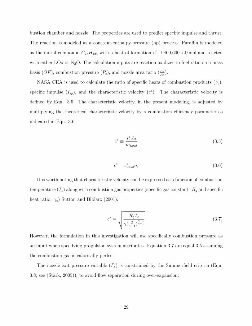
bustion chamber and nozzle. The properties are used to predict specific impulse and thrust.

The reaction is modeled as a constant-enthalpy-pressure (hp) process. Paraffin is modeled

as the initial compound C73H124 with a heat of formation of -1,860,600 kJ/mol and reacted

with either LOx or N2O. The calculation inputs are reaction oxidizer-to-fuel ratio on a mass

basis (OF ), combustion pressure (Pc), and nozzle area ratio (AeAt

).

NASA CEA is used to calculate the ratio of specific heats of combustion products (γc),

specific impulse (Isp), and the characteristic velocity (c∗). The characteristic velocity is

defined by Eqn. 3.5. The characteristic velocity, in the present modeling, is adjusted by

multiplying the theoretical characteristic velocity by a combustion efficiency parameter as

indicated in Eqn. 3.6.

c∗ ≡ PcAtmtotal

(3.5)

c∗ = c∗idealηc (3.6)

It is worth noting that characteristic velocity can be expressed as a function of combustion

temperature (Tc) along with combustion gas properties (specific gas constant: Rg and specific

heat ratio: γc) Sutton and Biblarz (2001):

c∗ =

√√√√ RgTc

γ( 2γ+1

)γ+1γ−1

(3.7)

However, the formulation in this investigation will use specifically combustion pressure as

an input when specifying propulsion system attributes. Equation 3.7 are equal 3.5 assuming

the combustion gas is calorically perfect.

The nozzle exit pressure variable (Pe) is constrained by the Summerfield criteria (Eqn.

3.8; see (Stark, 2005)), to avoid flow separation during over-expansion:

29

Pe > 0.4Pamb (3.8)

Four different methods of calculating the relevant propulsion system quantities are ex-

plored in this study. The first method, Method 1, uses only the equilibrium reaction proper-

ties in the combustion chamber. Method 1 assumes constant stagnation enthalpy, constant

specific heat ratio (calorically perfect), and constant entropy in the nozzle expansion to pre-

dict theoretical properties. All the remaining methods do not use the calorically perfect gas

assumption, but continue to use the isentropic assumption in the nozzle flow. Method 2

assumes that the chemical reaction is frozen in the combustion chamber, similar to Method

1, but the expanded gas is calorically imperfect. Method 3 is an extension, where the re-

action is allowed to equilibrate and the reaction is frozen at the nozzle throat. Method 4

is allowed to equilibrate along the entire length of the nozzle. Method 4 is referred to as

shifting equilibrium by other researchers (Castellini, 2012).

Each method’s implementation will be assessed. The methods are re-listed below:

1. Calorically perfect, frozen in the chamber

2. Calorically imperfect, frozen in the chamber

3. Calorically imperfect, frozen at the nozzle throat

4. Calorically imperfect, shifting equilibrium

Method 1: Calorically Perfect Gas

Method 1, using calorically perfect gas, was found to be commonly used in the literature

surveyed (Miranda, 2015; Casalino et al., 2019a). The prevalence of Method 1 is attributed

to its relative simplicity, as the other methods require the nozzle area ratio as an input.

This method first assumes that the specific heat ratio of combustion products is constant

between inefficient combustion and efficient combustion. After assuming constant specific

heat ratio and stagnation temperature, the thrust coefficient and area ratio for the design

30

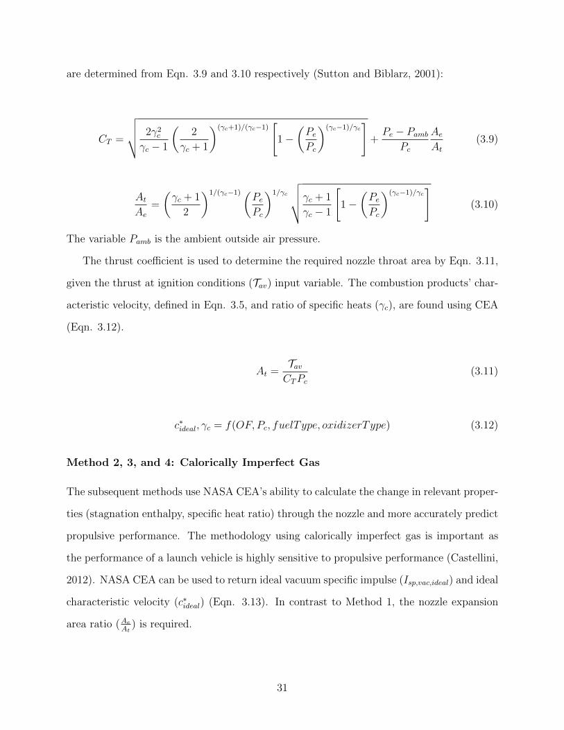
are determined from Eqn. 3.9 and 3.10 respectively (Sutton and Biblarz, 2001):

CT =

√√√√ 2γ2c

γc − 1

(2

γc + 1

)(γc+1)/(γc−1)[

1−(PePc

)(γc−1)/γc]

+Pe − Pamb

Pc

AeAt

(3.9)

AtAe

=

(γc + 1

2

)1/(γc−1)(PePc

)1/γc

√√√√γc + 1

γc − 1

[1−

(PePc

)(γc−1)/γc]

(3.10)

The variable Pamb is the ambient outside air pressure.

The thrust coefficient is used to determine the required nozzle throat area by Eqn. 3.11,

given the thrust at ignition conditions (Tav) input variable. The combustion products’ char-

acteristic velocity, defined in Eqn. 3.5, and ratio of specific heats (γc), are found using CEA

(Eqn. 3.12).

At =TavCTPc

(3.11)

c∗ideal, γc = f(OF, Pc, fuelType, oxidizerType) (3.12)

Method 2, 3, and 4: Calorically Imperfect Gas

The subsequent methods use NASA CEA’s ability to calculate the change in relevant proper-

ties (stagnation enthalpy, specific heat ratio) through the nozzle and more accurately predict

propulsive performance. The methodology using calorically imperfect gas is important as

the performance of a launch vehicle is highly sensitive to propulsive performance (Castellini,

2012). NASA CEA can be used to return ideal vacuum specific impulse (Isp,vac,ideal) and ideal

characteristic velocity (c∗ideal) (Eqn. 3.13). In contrast to Method 1, the nozzle expansion

area ratio (AeAt

) is required.

31

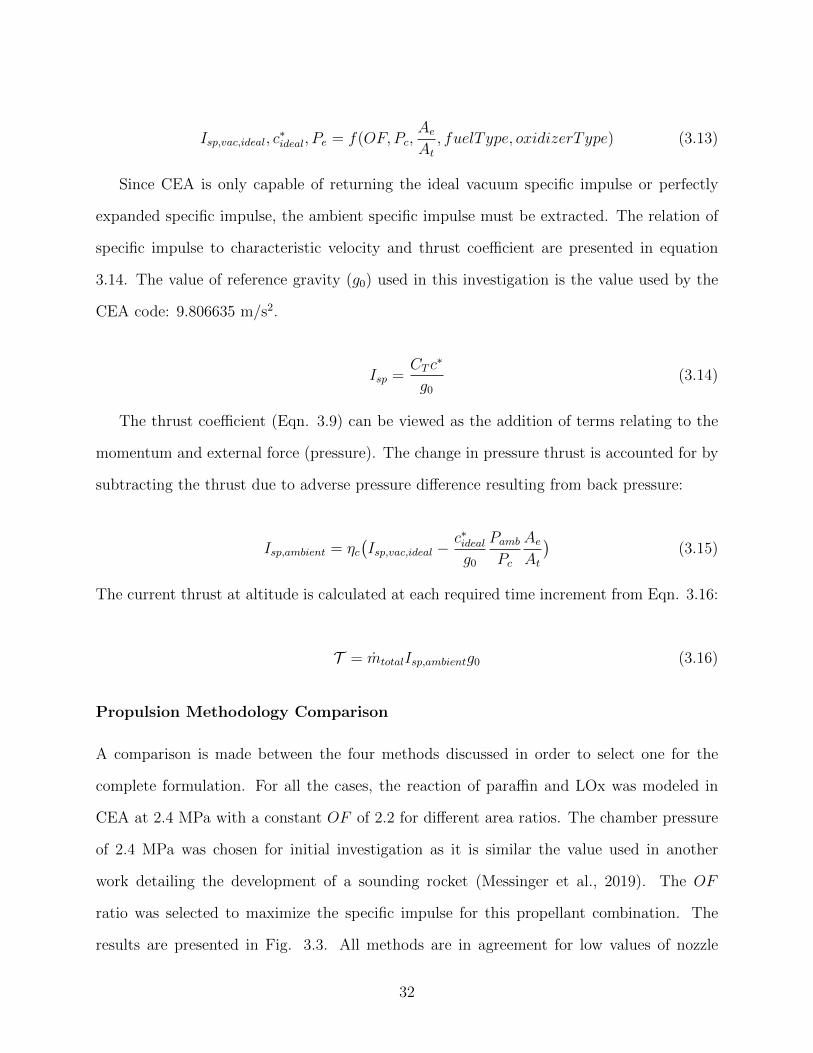
Isp,vac,ideal, c∗ideal, Pe = f(OF, Pc,

AeAt, fuelType, oxidizerType) (3.13)

Since CEA is only capable of returning the ideal vacuum specific impulse or perfectly

expanded specific impulse, the ambient specific impulse must be extracted. The relation of

specific impulse to characteristic velocity and thrust coefficient are presented in equation

3.14. The value of reference gravity (g0) used in this investigation is the value used by the

CEA code: 9.806635 m/s2.

Isp =CT c

∗

g0

(3.14)

The thrust coefficient (Eqn. 3.9) can be viewed as the addition of terms relating to the

momentum and external force (pressure). The change in pressure thrust is accounted for by

subtracting the thrust due to adverse pressure difference resulting from back pressure:

Isp,ambient = ηc(Isp,vac,ideal −

c∗idealg0

PambPc

AeAt

)(3.15)

The current thrust at altitude is calculated at each required time increment from Eqn. 3.16:

T = mtotalIsp,ambientg0 (3.16)

Propulsion Methodology Comparison

A comparison is made between the four methods discussed in order to select one for the

complete formulation. For all the cases, the reaction of paraffin and LOx was modeled in

CEA at 2.4 MPa with a constant OF of 2.2 for different area ratios. The chamber pressure

of 2.4 MPa was chosen for initial investigation as it is similar the value used in another

work detailing the development of a sounding rocket (Messinger et al., 2019). The OF

ratio was selected to maximize the specific impulse for this propellant combination. The

results are presented in Fig. 3.3. All methods are in agreement for low values of nozzle

32

area ratio. Method 1 predicts relatively high performance for high area ratio nozzles. After

investigation, the high performance was attributed to the low specific heat ratio that typically

changes during expansions, for this reason this formulation was not used. The shifting

equilibrium (Method 4) results in the highest predicted performance (Isp) while the frozen

reaction at the chamber, with calorically imperfect gas, predicts the lowest performance. In

practice, the theoretical performance is bounded by the frozen in the chamber, and shifting

equilibrium predictions. Method 3 is a compromise between the under prediction of Method

2 and optimism of Method 4. Method 3 is typically used to report combustion efficiencies

(Castellini, 2012) so will be adopted here and used going forward.

0 20 40 60 80 100Nozzle area ratio [Ae/At]

220

240

260

280

300

320

340

360

380

Vacu

um sp

ecifi

c im

pulse

[s]

Method 1Method 2Method 3Method 4

Figure 3.3: Vacuum specific impulse with different formulations for paraffin/LOx at Pc =2.4 MPa, OF = 2.2

First/main Stage Nozzle Formulation

For first-stage nozzles, the above formulation is used with nozzle exit pressure provided

as an input constrained by the flow separation criteria. Since a calorically imperfect gas

33

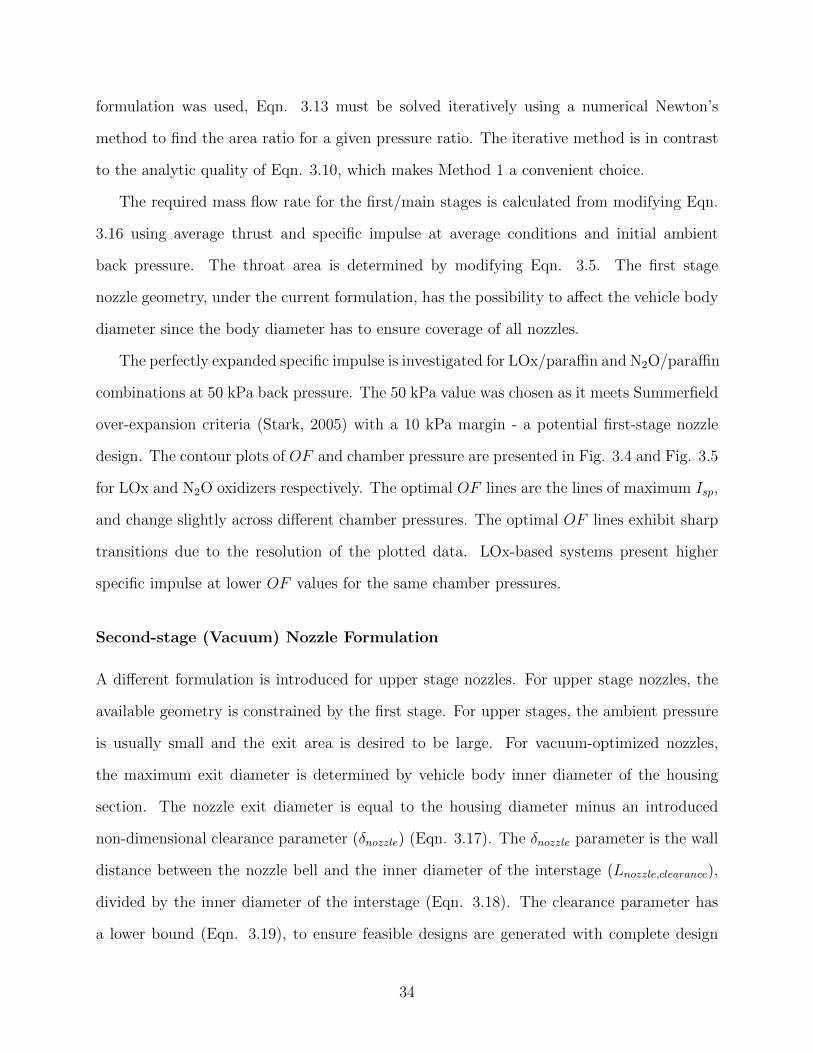
formulation was used, Eqn. 3.13 must be solved iteratively using a numerical Newton’s

method to find the area ratio for a given pressure ratio. The iterative method is in contrast

to the analytic quality of Eqn. 3.10, which makes Method 1 a convenient choice.

The required mass flow rate for the first/main stages is calculated from modifying Eqn.

3.16 using average thrust and specific impulse at average conditions and initial ambient

back pressure. The throat area is determined by modifying Eqn. 3.5. The first stage

nozzle geometry, under the current formulation, has the possibility to affect the vehicle body

diameter since the body diameter has to ensure coverage of all nozzles.

The perfectly expanded specific impulse is investigated for LOx/paraffin and N2O/paraffin

combinations at 50 kPa back pressure. The 50 kPa value was chosen as it meets Summerfield

over-expansion criteria (Stark, 2005) with a 10 kPa margin - a potential first-stage nozzle

design. The contour plots of OF and chamber pressure are presented in Fig. 3.4 and Fig. 3.5

for LOx and N2O oxidizers respectively. The optimal OF lines are the lines of maximum Isp,

and change slightly across different chamber pressures. The optimal OF lines exhibit sharp

transitions due to the resolution of the plotted data. LOx-based systems present higher

specific impulse at lower OF values for the same chamber pressures.

Second-stage (Vacuum) Nozzle Formulation

A different formulation is introduced for upper stage nozzles. For upper stage nozzles, the

available geometry is constrained by the first stage. For upper stages, the ambient pressure

is usually small and the exit area is desired to be large. For vacuum-optimized nozzles,

the maximum exit diameter is determined by vehicle body inner diameter of the housing

section. The nozzle exit diameter is equal to the housing diameter minus an introduced

non-dimensional clearance parameter (δnozzle) (Eqn. 3.17). The δnozzle parameter is the wall

distance between the nozzle bell and the inner diameter of the interstage (Lnozzle,clearance),

divided by the inner diameter of the interstage (Eqn. 3.18). The clearance parameter has

a lower bound (Eqn. 3.19), to ensure feasible designs are generated with complete design

34

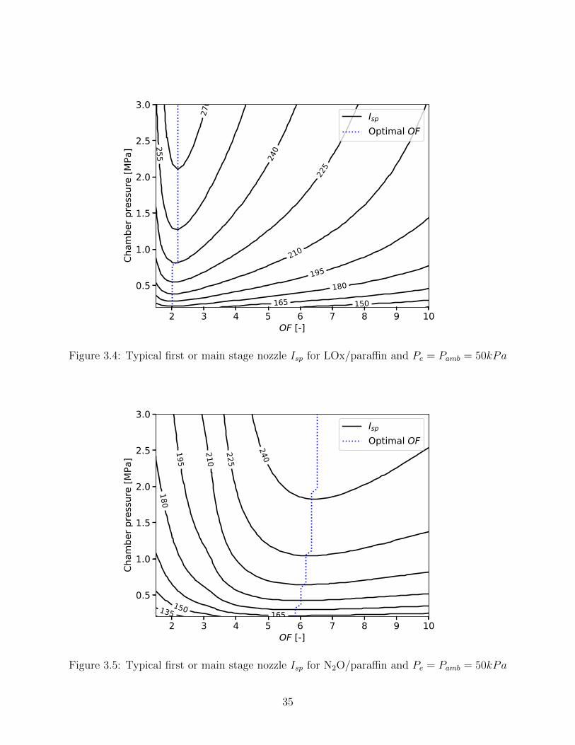
2 3 4 5 6 7 8 9 10OF [-]

0.5

1.0

1.5

2.0

2.5

3.0

Cham

ber p

ress

ure

[MPa

]

150165180

195210

225

240255

270

Isp

Optimal OF

Figure 3.4: Typical first or main stage nozzle Isp for LOx/paraffin and Pe = Pamb = 50kPa

2 3 4 5 6 7 8 9 10OF [-]

0.5

1.0

1.5

2.0

2.5

3.0

Cham

ber p

ress

ure

[MPa

]

135150 165

180195

210

225

240

Isp

Optimal OF

Figure 3.5: Typical first or main stage nozzle Isp for N2O/paraffin and Pe = Pamb = 50kPa

35

freedom to make any scale nozzle, within physical bounds. Upper stage nozzle throat area

is determined iteratively with Newton’s method with nominal vacuum thrust and exit area

constraints (Eqns. 3.13, 3.15, and 3.16). The mass flow rate is calculated similarly to first-

stage nozzles by modifying Eqn. 3.16 using average thrust and specific impulse at average

conditions and zero initial back pressure assumed.

Dexit = (ID)interstage(1− 2δnozzle) (3.17)

δnozzle =Lnozzle,clearance(ID)interstage

(3.18)

0.05 ≤ δnozzle < 0.5 (3.19)

Propellant Masses and Geometry

The oxidizer and fuel nominal average mass flow rates are determined using the time-averaged

oxidizer-to-fuel ratio (Eqn. 3.20). The variables mox and mf are the oxidizer and fuel mass

flow rates respectively, and mtotal is the total combined mass flow rate with the over bar

symbolizing a time-averaged quantity.

mox = mtotal − mf =mtotal

1 + (1/OFav)(3.20)

The individual propellant masses are determined by the average mass flow rates and burn

time, Eqn. 3.21. The subscript i denotes an arbitrary propellant (fuel or oxidizer).

mi = mi · tb (3.21)

A single-port, circular-cylinder fuel grain geometry is used in this study. The fuel radius

regression-rate (rf ) power law, of the form shown by Eqn. 3.22, is used (Karabeyoglu et al.,

36

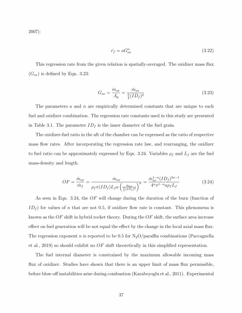
2007):

rf = aGnox (3.22)

This regression rate from the given relation is spatially-averaged. The oxidizer mass flux

(Gox) is defined by Eqn. 3.23:

Gox =mox

Ap=

moxπ4(IDf )2

(3.23)

The parameters a and n are empirically determined constants that are unique to each

fuel and oxidizer combination. The regression rate constants used in this study are presented

in Table 3.1. The parameter IDf is the inner diameter of the fuel grain.

The oxidizer-fuel ratio in the aft of the chamber can be expressed as the ratio of respective

mass flow rates. After incorporating the regression rate law, and rearranging, the oxidizer

to fuel ratio can be approximately expressed by Eqn. 3.24. Variables ρf and Lf are the fuel

mass-density and length.

OF =mox

mf

=mox

ρfπ(IDf )Lfa(

moxπ4

(IDf )2

)n =m1−nox (IDf )

2n−1

4nπ1−naρfLf(3.24)

As seen in Eqn. 3.24, the OF will change during the duration of the burn (function of

IDf ) for values of n that are not 0.5, if oxidizer flow rate is constant. This phenomena is

known as the OF shift in hybrid rocket theory. During the OF shift, the surface area increase

effect on fuel generation will be not equal the effect by the change in the local axial mass flux.

The regression exponent n is reported to be 0.5 for N2O/paraffin combinations (Paccagnella

et al., 2019) so should exhibit no OF shift theoretically in this simplified representation.

The fuel internal diameter is constrained by the maximum allowable incoming mass

flux of oxidizer. Studies have shown that there is an upper limit of mass flux permissible,

before blow-off instabilities arise during combustion (Karabeyoglu et al., 2011). Experimental

37

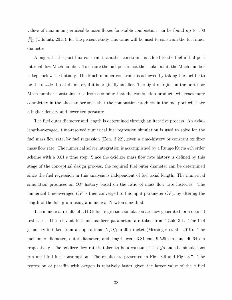
values of maximum permissible mass fluxes for stable combustion can be found up to 500

kgm2s

(Uddanti, 2015), for the present study this value will be used to constrain the fuel inner

diameter.

Along with the port flux constraint, another constraint is added to the fuel initial port

internal flow Mach number. To ensure the fuel port is not the choke point, the Mach number

is kept below 1.0 initially. The Mach number constraint is achieved by taking the fuel ID to

be the nozzle throat diameter, if it is originally smaller. The tight margins on the port flow

Mach number constraint arise from assuming that the combustion products will react more

completely in the aft chamber such that the combustion products in the fuel port will have

a higher density and lower temperature.

The fuel outer diameter and length is determined through an iterative process. An axial-

length-averaged, time-resolved numerical fuel regression simulation is used to solve for the

fuel mass flow rate, by fuel regression (Eqn. 3.22), given a time-history or constant oxidizer

mass flow rate. The numerical solver integration is accomplished by a Runge-Kutta 4th order

scheme with a 0.01 s time step. Since the oxidizer mass flow rate history is defined by this

stage of the conceptual design process, the required fuel outer diameter can be determined

since the fuel regression in this analysis is independent of fuel axial length. The numerical

simulation produces an OF history based on the ratio of mass flow rate histories. The

numerical time-averaged OF is then converged to the input parameter OFav by altering the

length of the fuel grain using a numerical Newton’s method.

The numerical results of a HRE fuel regression simulation are now generated for a defined

test case. The relevant fuel and oxidizer parameters are taken from Table 3.1. The fuel

geometry is taken from an operational N2O/paraffin rocket (Messinger et al., 2019). The

fuel inner diameter, outer diameter, and length were 3.81 cm, 9.525 cm, and 40.64 cm

respectively. The oxidizer flow rate is taken to be a constant 1.2 kg/s and the simulations

run until full fuel consumption. The results are presented in Fig. 3.6 and Fig. 3.7. The

regression of paraffin with oxygen is relatively faster given the larger value of the a fuel

38

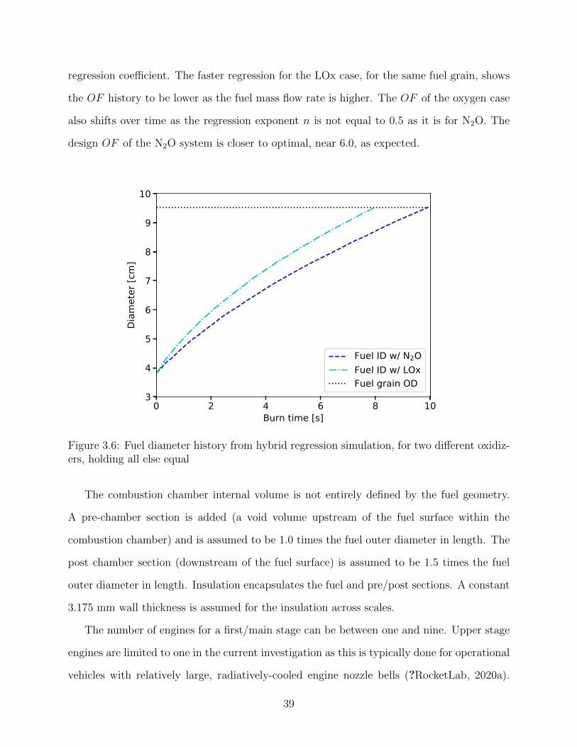
regression coefficient. The faster regression for the LOx case, for the same fuel grain, shows

the OF history to be lower as the fuel mass flow rate is higher. The OF of the oxygen case

also shifts over time as the regression exponent n is not equal to 0.5 as it is for N2O. The

design OF of the N2O system is closer to optimal, near 6.0, as expected.

0 2 4 6 8 10Burn time [s]

3

4

5

6

7

8

9

10

Diam

eter

[cm

]

Fuel ID w/ N2OFuel ID w/ LOxFuel grain OD

Figure 3.6: Fuel diameter history from hybrid regression simulation, for two different oxidiz-ers, holding all else equal

The combustion chamber internal volume is not entirely defined by the fuel geometry.

A pre-chamber section is added (a void volume upstream of the fuel surface within the

combustion chamber) and is assumed to be 1.0 times the fuel outer diameter in length. The

post chamber section (downstream of the fuel surface) is assumed to be 1.5 times the fuel

outer diameter in length. Insulation encapsulates the fuel and pre/post sections. A constant

3.175 mm wall thickness is assumed for the insulation across scales.

The number of engines for a first/main stage can be between one and nine. Upper stage

engines are limited to one in the current investigation as this is typically done for operational

vehicles with relatively large, radiatively-cooled engine nozzle bells (?RocketLab, 2020a).

39

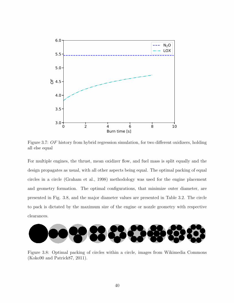
0 2 4 6 8 10Burn time [s]

3.0

3.5

4.0

4.5

5.0

5.5

6.0

OF

N2OLOX

Figure 3.7: OF history from hybrid regression simulation, for two different oxidizers, holdingall else equal

For multiple engines, the thrust, mean oxidizer flow, and fuel mass is split equally and the

design propagates as usual, with all other aspects being equal. The optimal packing of equal

circles in a circle (Graham et al., 1998) methodology was used for the engine placement

and geometry formation. The optimal configurations, that minimize outer diameter, are

presented in Fig. 3.8, and the major diameter values are presented in Table 3.2. The circle

to pack is dictated by the maximum size of the engine or nozzle geometry with respective

clearances.

Figure 3.8: Optimal packing of circles within a circle, images from Wikimedia Commons(Koko90 and Patrick87, 2011).

40

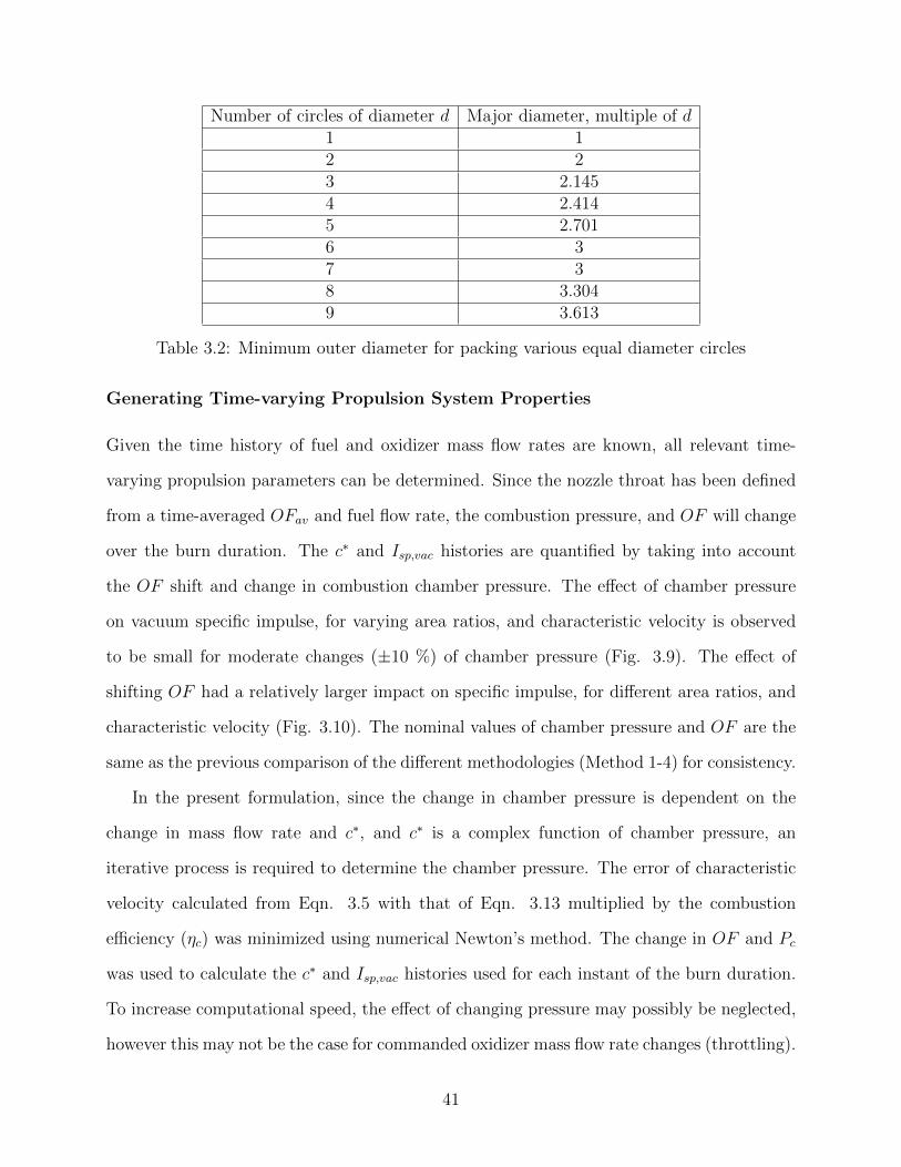
Number of circles of diameter d Major diameter, multiple of d1 12 23 2.1454 2.4145 2.7016 37 38 3.3049 3.613

Table 3.2: Minimum outer diameter for packing various equal diameter circles

Generating Time-varying Propulsion System Properties

Given the time history of fuel and oxidizer mass flow rates are known, all relevant time-

varying propulsion parameters can be determined. Since the nozzle throat has been defined

from a time-averaged OFav and fuel flow rate, the combustion pressure, and OF will change

over the burn duration. The c∗ and Isp,vac histories are quantified by taking into account

the OF shift and change in combustion chamber pressure. The effect of chamber pressure

on vacuum specific impulse, for varying area ratios, and characteristic velocity is observed

to be small for moderate changes (±10 %) of chamber pressure (Fig. 3.9). The effect of

shifting OF had a relatively larger impact on specific impulse, for different area ratios, and

characteristic velocity (Fig. 3.10). The nominal values of chamber pressure and OF are the

same as the previous comparison of the different methodologies (Method 1-4) for consistency.

In the present formulation, since the change in chamber pressure is dependent on the

change in mass flow rate and c∗, and c∗ is a complex function of chamber pressure, an

iterative process is required to determine the chamber pressure. The error of characteristic

velocity calculated from Eqn. 3.5 with that of Eqn. 3.13 multiplied by the combustion

efficiency (ηc) was minimized using numerical Newton’s method. The change in OF and Pc

was used to calculate the c∗ and Isp,vac histories used for each instant of the burn duration.

To increase computational speed, the effect of changing pressure may possibly be neglected,

however this may not be the case for commanded oxidizer mass flow rate changes (throttling).

41

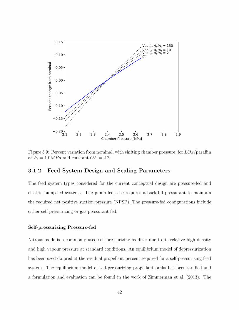
2.1 2.2 2.3 2.4 2.5 2.6 2.7 2.8 2.9Chamber Pressure [MPa]

0.20

0.15

0.10

0.05

0.00

0.05

0.10

0.15

Perc

ent c

hang

e fro

m n

omin

al Vac Is, Ae/At = 2 Vac Is, Ae/At = 10 Vac Is, Ae/At = 150

C *

Figure 3.9: Percent variation from nominal, with shifting chamber pressure, for LOx/paraffinat Pc = 1.0MPa and constant OF = 2.2

3.1.2 Feed System Design and Scaling Parameters

The feed system types considered for the current conceptual design are pressure-fed and

electric pump-fed systems. The pump-fed case requires a back-fill pressurant to maintain

the required net positive suction pressure (NPSP). The pressure-fed configurations include

either self-pressurizing or gas pressurant-fed.

Self-pressurizing Pressure-fed

Nitrous oxide is a commonly used self-pressurizing oxidizer due to its relative high density

and high vapour pressure at standard conditions. An equilibrium model of depressurization

has been used do predict the residual propellant percent required for a self-pressurizing feed

system. The equilibrium model of self-pressurizing propellant tanks has been studied and

a formulation and evaluation can be found in the work of Zimmerman et al. (2013). The

42

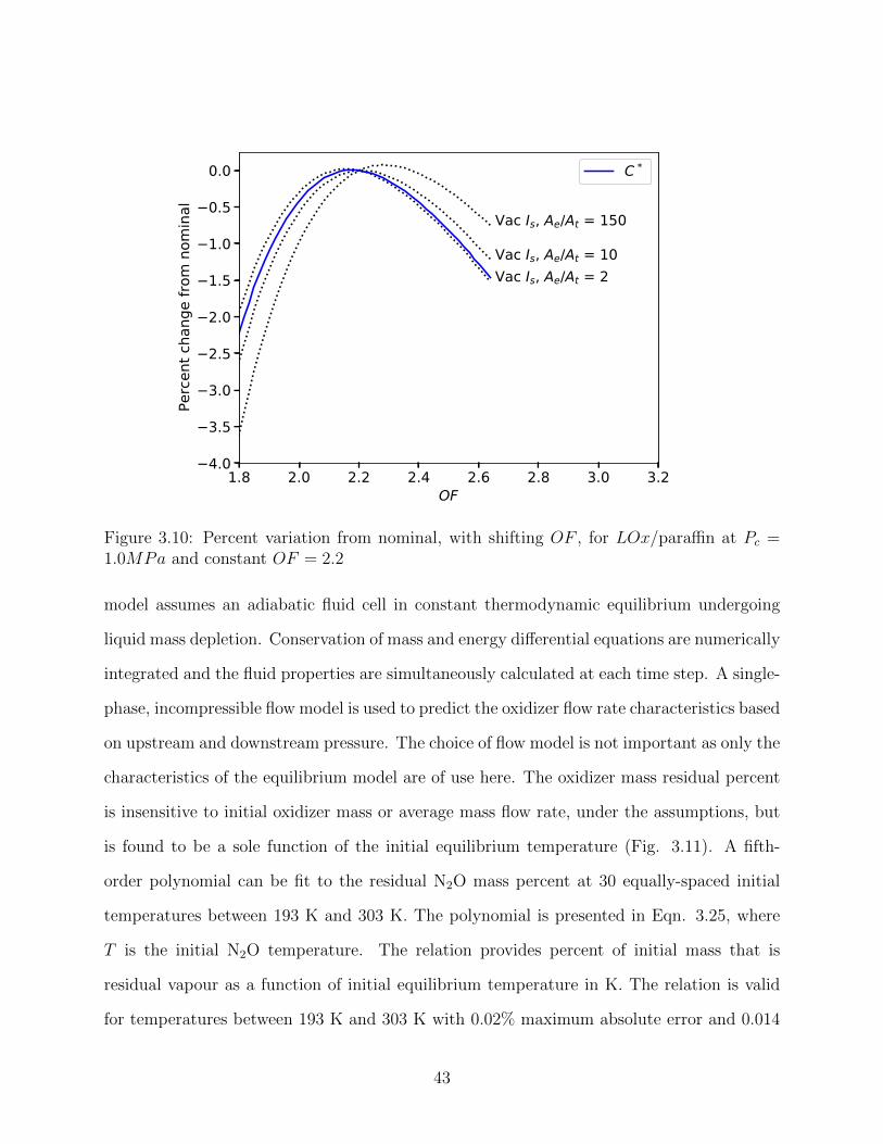
1.8 2.0 2.2 2.4 2.6 2.8 3.0 3.2OF

4.0

3.5

3.0

2.5

2.0

1.5

1.0

0.5

0.0Pe

rcen

t cha

nge

from

nom

inal

Vac Is, Ae/At = 2 Vac Is, Ae/At = 10

Vac Is, Ae/At = 150

C *

Figure 3.10: Percent variation from nominal, with shifting OF , for LOx/paraffin at Pc =1.0MPa and constant OF = 2.2

model assumes an adiabatic fluid cell in constant thermodynamic equilibrium undergoing

liquid mass depletion. Conservation of mass and energy differential equations are numerically

integrated and the fluid properties are simultaneously calculated at each time step. A single-

phase, incompressible flow model is used to predict the oxidizer flow rate characteristics based

on upstream and downstream pressure. The choice of flow model is not important as only the

characteristics of the equilibrium model are of use here. The oxidizer mass residual percent

is insensitive to initial oxidizer mass or average mass flow rate, under the assumptions, but

is found to be a sole function of the initial equilibrium temperature (Fig. 3.11). A fifth-

order polynomial can be fit to the residual N2O mass percent at 30 equally-spaced initial

temperatures between 193 K and 303 K. The polynomial is presented in Eqn. 3.25, where

T is the initial N2O temperature. The relation provides percent of initial mass that is

residual vapour as a function of initial equilibrium temperature in K. The relation is valid

for temperatures between 193 K and 303 K with 0.02% maximum absolute error and 0.014

43

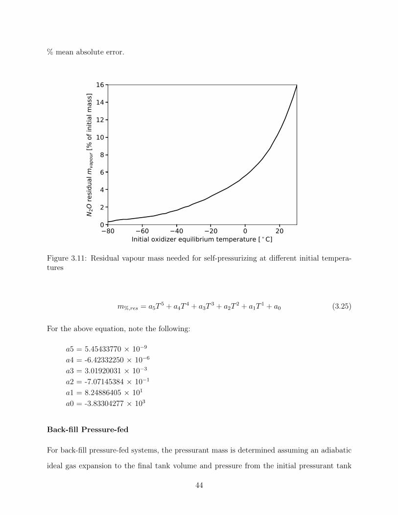
% mean absolute error.

80 60 40 20 0 20Initial oxidizer equilibrium temperature [ C]

0

2

4

6

8

10

12

14

16N

2O re

sidua

l mva

pour

[% o

f ini

tial m

ass]

Figure 3.11: Residual vapour mass needed for self-pressurizing at different initial tempera-tures

m%,res = a5T5 + a4T

4 + a3T3 + a2T

2 + a1T1 + a0 (3.25)

For the above equation, note the following:

a5 = 5.45433770 × 10−9

a4 = -6.42332250 × 10−6

a3 = 3.01920031 × 10−3

a2 = -7.07145384 × 10−1

a1 = 8.24886405 × 101

a0 = -3.83304277 × 103

Back-fill Pressure-fed

For back-fill pressure-fed systems, the pressurant mass is determined assuming an adiabatic

ideal gas expansion to the final tank volume and pressure from the initial pressurant tank

44

pressure and temperature. The pressurant mass is calculated from Eqn. 3.26 assuming ideal

gas properties during depressurization (Castellini, 2012). The resulting mass is multiplied

by a factor, cpg, to provide a margin. A value of 1.2 is used for cpg in this study, as was used

by Castellini (2012).

mpg = cpgPox–VoxRpgT1,pg

(γpg

1− PoxP1,pg

)(3.26)

The initial temperature and pressure of the pressurant gas are design parameters. The

pressurant density is found by an equation of state in CoolProp (Bell et al., 2014). The

volume requirements are calculated from the required mass.

Electric Pump-fed

The electric pump feed system is defined by the power requirements of the pump and batter-

ies, and the energy requirements of the batteries, while taking into account pump efficiency.

The pump instantaneous power is expressed in Eqn. 3.27 :

Pep =mox∆Pepρoxηep

(3.27)

Where Pep is the electric pump required power, ηep is the electric pump efficiency, and ∆Pep

is the difference between the pump inlet and outlet pressure, or oxidizer tank and injector

inlet.

The total energy is the temporal integral of the power used over the burn duration 3.28

Eep =

∫ tb

0

Pepdt (3.28)

The battery mass (mb) is determined from an empirical battery energy density (δbe) and

battery power density( δbp). The battery mass is determined from the maximum of the

energy limited or power limited case, as per Eqn. 3.29:

45

mb = max(Pep,maxδbp

,Eepδbe

) (3.29)

The pump mass is calculated based on a pump mass estimating relationship assuming

a constant pump power density (δep) across different engine sizes (power and flow rate re-

quirements) (Eqn. 3.30). The pump power density parameter captures the pump housing,

electric motor, and inverter which can all be taken as a a function of the power requirement

(Kwak et al., 2018). Values adapted from (Kwak et al., 2018; Gegeoglu et al., 2019; Casalino

et al., 2019b) are presented in Table 3.3 for use in this thesis.

mep =Pep,maxδep

(3.30)

The net positive suction pressure (NPSP) is the absolute pressure at the inlet eye of the

centrifugal pump (Eqn. 3.31). The available NPSP (NPSPA) is a function of pressurant

gas pressure (Ppg), static pressure in the oxidizer tank, and the vapour pressure of the

oxidizer (Pvap,ox). Where the static pressure in the oxidizer tank is equal to the following

expression: ρox|−→a |hox, and where hox is the current liquid level height and |−→a | is the apparent

acceleration.

NPSPA = Ppg + ρox|−→a |hox − Pvap,ox (3.31)

The available NPSP is required to be below a certain value to avoid cavitation during

the operation of the electric pump in order to prevent significant mechanical wear to the

impeller. The value of NPSPR is dictated by the detailed design of the impeller; a constant

value is assumed based on existing literature values (Campbell and Farquhar, 1973).

NPSPA ≥ NPSPR (3.32)

46

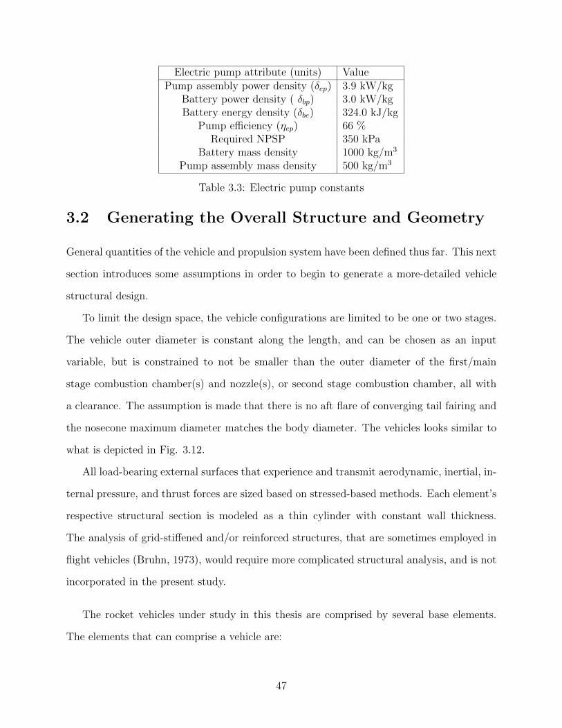
Electric pump attribute (units) ValuePump assembly power density (δep) 3.9 kW/kg

Battery power density ( δbp) 3.0 kW/kgBattery energy density (δbe) 324.0 kJ/kg

Pump efficiency (ηep) 66 %Required NPSP 350 kPa

Battery mass density 1000 kg/m3

Pump assembly mass density 500 kg/m3

Table 3.3: Electric pump constants

3.2 Generating the Overall Structure and Geometry

General quantities of the vehicle and propulsion system have been defined thus far. This next

section introduces some assumptions in order to begin to generate a more-detailed vehicle

structural design.

To limit the design space, the vehicle configurations are limited to be one or two stages.

The vehicle outer diameter is constant along the length, and can be chosen as an input

variable, but is constrained to not be smaller than the outer diameter of the first/main

stage combustion chamber(s) and nozzle(s), or second stage combustion chamber, all with

a clearance. The assumption is made that there is no aft flare of converging tail fairing and

the nosecone maximum diameter matches the body diameter. The vehicles looks similar to

what is depicted in Fig. 3.12.

All load-bearing external surfaces that experience and transmit aerodynamic, inertial, in-

ternal pressure, and thrust forces are sized based on stressed-based methods. Each element’s

respective structural section is modeled as a thin cylinder with constant wall thickness.

The analysis of grid-stiffened and/or reinforced structures, that are sometimes employed in

flight vehicles (Bruhn, 1973), would require more complicated structural analysis, and is not

incorporated in the present study.

The rocket vehicles under study in this thesis are comprised by several base elements.

The elements that can comprise a vehicle are:

47

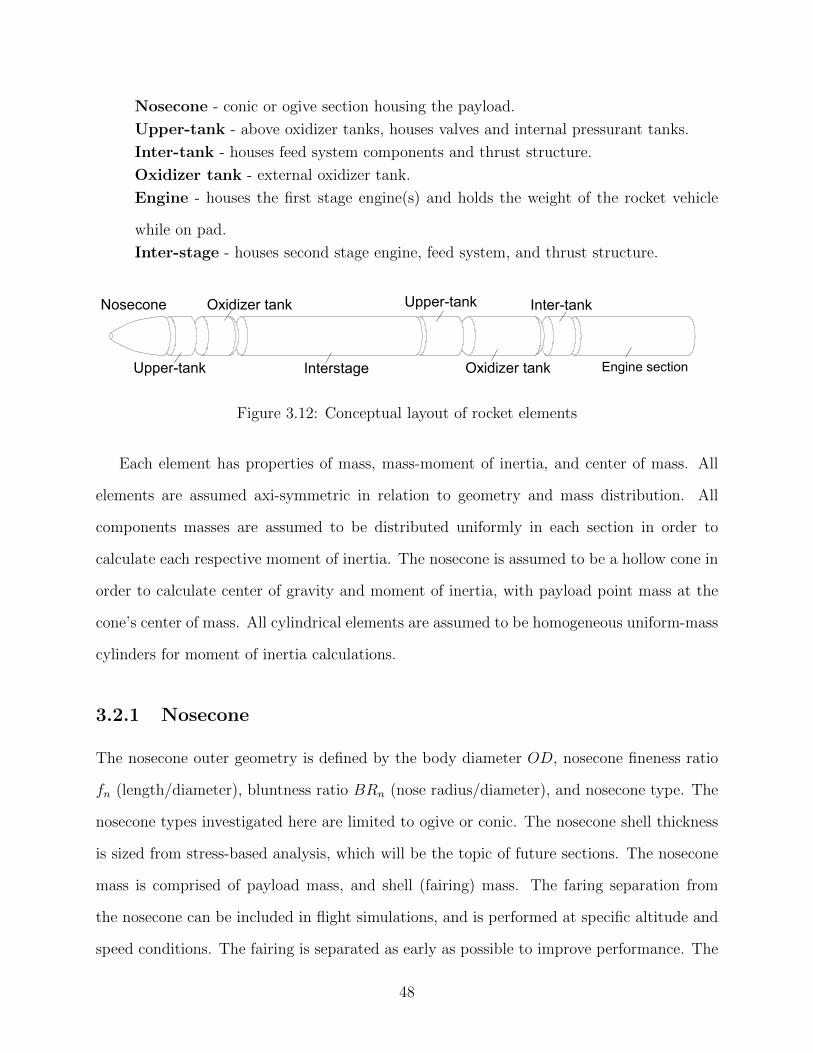
Nosecone - conic or ogive section housing the payload.

Upper-tank - above oxidizer tanks, houses valves and internal pressurant tanks.

Inter-tank - houses feed system components and thrust structure.

Oxidizer tank - external oxidizer tank.

Engine - houses the first stage engine(s) and holds the weight of the rocket vehicle

while on pad.

Inter-stage - houses second stage engine, feed system, and thrust structure.

Upper-tank

Nosecone Oxidizer tank

Interstage

Upper-tank

Oxidizer tank

Inter-tank

Engine section

Figure 3.12: Conceptual layout of rocket elements

Each element has properties of mass, mass-moment of inertia, and center of mass. All

elements are assumed axi-symmetric in relation to geometry and mass distribution. All

components masses are assumed to be distributed uniformly in each section in order to

calculate each respective moment of inertia. The nosecone is assumed to be a hollow cone in

order to calculate center of gravity and moment of inertia, with payload point mass at the

cone’s center of mass. All cylindrical elements are assumed to be homogeneous uniform-mass

cylinders for moment of inertia calculations.

3.2.1 Nosecone

The nosecone outer geometry is defined by the body diameter OD, nosecone fineness ratio

fn (length/diameter), bluntness ratio BRn (nose radius/diameter), and nosecone type. The

nosecone types investigated here are limited to ogive or conic. The nosecone shell thickness

is sized from stress-based analysis, which will be the topic of future sections. The nosecone

mass is comprised of payload mass, and shell (fairing) mass. The faring separation from

the nosecone can be included in flight simulations, and is performed at specific altitude and

speed conditions. The fairing is separated as early as possible to improve performance. The

48

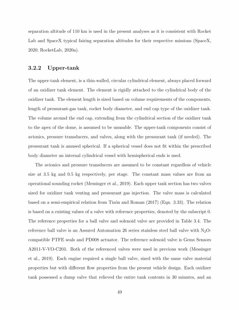
separation altitude of 110 km is used in the present analyses as it is consistent with Rocket

Lab and SpaceX typical fairing separation altitudes for their respective missions (SpaceX,

2020; RocketLab, 2020a).

3.2.2 Upper-tank

The upper-tank element, is a thin-walled, circular cylindrical element, always placed forward

of an oxidizer tank element. The element is rigidly attached to the cylindrical body of the

oxidizer tank. The element length is sized based on volume requirements of the components,

length of pressurant-gas tank, rocket body diameter, and end cap type of the oxidizer tank.

The volume around the end cap, extending from the cylindrical section of the oxidizer tank

to the apex of the dome, is assumed to be unusable. The upper-tank components consist of

avionics, pressure transducers, and valves, along with the pressurant tank (if needed). The

pressurant tank is amused spherical. If a spherical vessel does not fit within the prescribed

body diameter an internal cylindrical vessel with hemispherical ends is used.

The avionics and pressure transducers are assumed to be constant regardless of vehicle

size at 3.5 kg and 0.5 kg respectively, per stage. The constant mass values are from an

operational sounding rocket (Messinger et al., 2019). Each upper tank section has two valves

sized for oxidizer tank venting and pressurant gas injection. The valve mass is calculated

based on a semi-empirical relation from Tizon and Roman (2017) (Eqn. 3.33). The relation

is based on a existing values of a valve with reference properties, denoted by the subscript 0.

The reference properties for a ball valve and solenoid valve are provided in Table 3.4. The

reference ball valve is an Assured Automation 26 series stainless steel ball valve with N2O-

compatible PTFE seals and PD008 actuator. The reference solenoid valve is Gems Sensors

A2011-V-VO-C203. Both of the referenced valves were used in previous work (Messinger

et al., 2019). Each engine required a single ball valve, sized with the same valve material

properties but with different flow properties from the present vehicle design. Each oxidizer

tank possessed a dump valve that relieved the entire tank contents in 30 minutes, and an

49

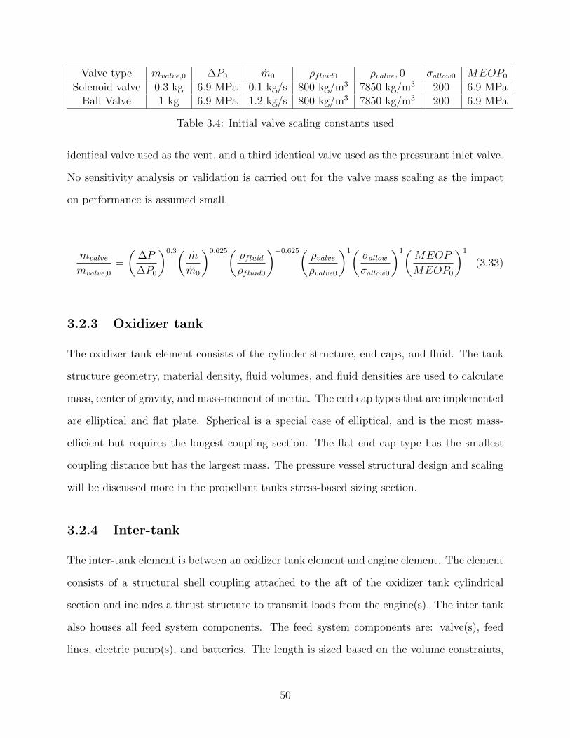
Valve type mvalve,0 ∆P0 m0 ρfluid0 ρvalve, 0 σallow0 MEOP0

Solenoid valve 0.3 kg 6.9 MPa 0.1 kg/s 800 kg/m3 7850 kg/m3 200 6.9 MPaBall Valve 1 kg 6.9 MPa 1.2 kg/s 800 kg/m3 7850 kg/m3 200 6.9 MPa

Table 3.4: Initial valve scaling constants used

identical valve used as the vent, and a third identical valve used as the pressurant inlet valve.

No sensitivity analysis or validation is carried out for the valve mass scaling as the impact

on performance is assumed small.

mvalve

mvalve,0

=

(∆P

∆P0

)0.3(m

m0

)0.625(ρfluidρfluid0

)−0.625(ρvalveρvalve0

)1(σallowσallow0

)1(MEOP

MEOP0

)1

(3.33)

3.2.3 Oxidizer tank

The oxidizer tank element consists of the cylinder structure, end caps, and fluid. The tank

structure geometry, material density, fluid volumes, and fluid densities are used to calculate

mass, center of gravity, and mass-moment of inertia. The end cap types that are implemented

are elliptical and flat plate. Spherical is a special case of elliptical, and is the most mass-

efficient but requires the longest coupling section. The flat end cap type has the smallest

coupling distance but has the largest mass. The pressure vessel structural design and scaling

will be discussed more in the propellant tanks stress-based sizing section.

3.2.4 Inter-tank

The inter-tank element is between an oxidizer tank element and engine element. The element

consists of a structural shell coupling attached to the aft of the oxidizer tank cylindrical

section and includes a thrust structure to transmit loads from the engine(s). The inter-tank

also houses all feed system components. The feed system components are: valve(s), feed

lines, electric pump(s), and batteries. The length is sized based on the volume constraints,

50

given the mass and density of internal components, and the body diameter. The mass is

comprised of the components mass and structural shell mass. The thrust structure cross-

sectional area is sized per engine assuming simple axial compression and the thrust structure

length spans the length housing the feed system components. It’s assumed that the thrust

structure section properties can be designed in such a way that material yield, and not

buckling, will be the failure mode. The feed system line flow area is sized based on a limit

design velocity and oxidizer volumetric flow per engine. The flow area, line pressure, and

inter-tank length provides the feed line mass per thin-walled pressure vessel theory, which

will be discussed in the structural analysis section.

3.2.5 Engine

The engine component consists of combustion chamber(s), fuel, nozzle(s), and a structural

shell that extends from the end of the inter-tank to the start of the nozzle(s). The engine

shell is sized to withstand the static load of the vehicle on the pad as well as the dynamic

flight loads. The overall element length is determined from the combustion chamber and

nozzle length.

The nozzle geometry is generated using the bell (parabolic) formulation outlined in Sutton

and Biblarz (2001). Given the throat diameter, exit diameter, and combustion chamber outer

diameter the nozzle contour can be fully defined. A straight 45◦ half angle converging section

is used that is tangent to the throat fillet and is coincident with the combustion chamber

outer diameter. Per the Sutton formulation, a 80% bell contour with an 8.5◦ exit half angle

is used. The throat fillet to parabola transition angle is 30◦. The throat aft and fore fillets

are 1.5 and 0.4 throat radii respectively. The non-zero nozzle exit angle contributes a 0.995

nozzle correction factor applied to the momentum thrust term in the thrust coefficient. A

nozzle contour with an area ratio of four, and inlet diameter of eight throat radii (rt), is

shown in Fig. 3.13.

The nozzle mass is determined from the addition of a nozzle MER from Miranda (2015)

51

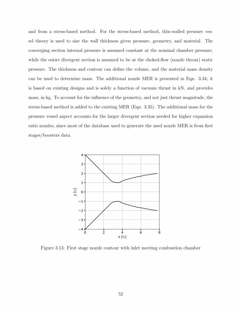
and from a stress-based method. For the stress-based method, thin-walled pressure ves-

sel theory is used to size the wall thickness given pressure, geometry, and material. The

converging section internal pressure is assumed constant at the nominal chamber pressure,

while the entire divergent section is assumed to be at the choked-flow (nozzle throat) static

pressure. The thickness and contour can define the volume, and the material mass density

can be used to determine mass. The additional nozzle MER is presented in Eqn. 3.34; it

is based on existing designs and is solely a function of vacuum thrust in kN, and provides

mass, in kg. To account for the influence of the geometry, and not just thrust magnitude, the

stress-based method is added to the existing MER (Eqn. 3.35). The additional mass for the

pressure vessel aspect accounts for the larger divergent section needed for higher expansion

ratio nozzles, since most of the database used to generate the used nozzle MER is from first

stages/boosters data.

0 2 4 6 8x [rt]

4

3

2

1

0

1

2

3

4

y [r t

]

Figure 3.13: First stage nozzle contour with inlet meeting combustion chamber

52

mnozzle,0 =

0.0006(Tvac)

2 − 0.3214(Tvac) + 263.82, Tvac > 200kN,+TV C

−0.0018(Tvac)2 + 1.004(Tvac)− 1.942, Tvac ≤ 200kN,+TV C

0.1605(Tvac)1.2466 Tvac ≤ 200kN

(3.34)

mnozzle = mnozzle,0 +mnozzle,pv (3.35)

3.2.6 Interstage

The interstage is connected to the lower stage upper-tank and connects to the upper stage

oxidizer tank. The interstage element inherits all attributes from the inter-tank element,

but only holds the components pertaining to the second stage. Interstages are only used

when more than one stage is simulated. The combustion chamber(s) and nozzle(s) mass and

length are incorporated in the element, along with all quantities that are contained in the

inter-tank element. The structural shell is jettisoned when staging occurs (i.e remains with

the first stage).

3.3 Aerodynamics

The aerodynamic forces on the vehicle, axial force (drag) and normal force (lift), are com-

puted for each element. The normal force distribution over the entire vehicle is used to

determine vehicle loads, stresses, and ultimately size vehicle components under assumed

structural failure criteria. The magnitude and resultant of the normal force is used to cal-

culate the required thrust vector to ensure static control can be obtained. The drag is used

to determine the axial force distribution and in the numerical flight simulation equations

of motion. This type of component-buildup method is used in other programs (Hammond,

2001), and is used for its computational speed over lattice/panel methods or computational

53

fluid dynamic (CFD) methods. The increase in computational speed comes with reduced

accuracy, but is necessary for large parametric or optimization studies.

This investigation incorporates the 1997 version of Missile Datcom (Blake, 1998). The

Missile Datcom source code was made publicly available in the supplementary material of

Design Methodologies for Space Transportation Systems by Hammond (2001). The aerody-

namic quantities used in this study are: the zero angle of attack drag coefficient (CD0), the

normal force derivative with angle of attack, at zero angle of attack (CNα), and the center

of pressure xcp at zero angle of attack.

The definition of the drag coefficient is presented here in Eqn. 3.36 and 3.37. Where ρ is

the local air density, U is the local airspeed magnitude, and Aref is the reference area based

on the diameter of the nosecone base-circle. The diameter will be constant along the axial

length of the vehicle in this investigation,

CD =D

12ρU2Aref

(3.36)

CD0 =D|(α=0)

12ρU2Aref

(3.37)

where q is the dynamic pressure:

q =1

2ρU2 (3.38)

For the geometry of the vehicles assumed in this study, the drag will only be comprised of

wave, friction and base (pressure) components (Eqn. 3.39):

CD = CDw + CDf + CDbase (3.39)

In this study the normal force will be determined, in the small angle of attack regime, as

a linear function of angle of attack, from Eqns. 3.40, 3.41, 3.42:

54

CN =N

12ρU2Aref

(3.40)

CN ≈∂CN∂α

∣∣∣∣(α=0)

α (3.41)

CNα =∂CN∂α

(3.42)

The center of pressure is defined by the following:

xcp =

∫x · P (x)dx∫P (x)dx

(3.43)

The center of pressure will be calculated using exclusively the normal forces since angle of

attack is assumed to be small. The center of pressure due to the finite discrete normal forces

is calculated with the following:

xcp =

∑ni xcp,i · CNα,i∑n

i CNα,i(3.44)

3.3.1 Nosecone: Wave Drag, Normal Force, and Center of Pres-

sure

The nosecone aerodynamic quantities are calculated using the methods contained in 1997

Missile Datcom. The methods use: The Second Order Shock Expansion (SOSE) theory,

Van Dyke Hybrid theory, and the Modified Newtonian theory (Blake, 1998). All three

methods are called directly from the compiled Datcom code. The SOSE method assumes

an attached oblique shock at the tip of the nosecone and subsequent expansions along the

length assuming each local change is conical. SOSE has been shown to have up to 20% error

for low supersonic flight Mach numbers (M ≤ 2.0), It is in this region Van Dyke Hybrid

theory is used (Blake, 1998). The SOSE method is used between Mach 2.0 and 6.0; beyond

55

Mach 6.0, the Modified Newtonian Theroy is used. Datcom uses a semi-empirical transonic

(Mach = 0.8 to Mach 1.2) method based on experimental data for ogive and conic noses

and nose-body combinations. The Datcom transonic method uses data from experiments by

Messerschmitt-Boelkow-Blohm (Messerchmitt-Boelkow-Blohm, 1970).

In this investigation, for a given nosecone type and geometry (fineness ratio, bluntness

ratio, and base diameter), a lookup table of aerodynamic coefficients is generated using

Datcom, to be linearly interpolated as required. The coefficients generated are center of

pressure (xcp), zero-angle-of-attack normal force derivative (CNα), and wave drag (CDw) at

flight Mach numbers from 0 to 20. The skin friction drag and base drag methods of Datcom

were not used, but similar methods are incorporated as needed. Datcom was not called

exclusively because it does not export the pressure distribution along the body (or element

CNα and xcp), information which is necessary to calculate more accurate loads and stresses.

Datcom instead only returns the center of pressure and coefficients for forces/moments acting

at the center of pressure. Calling Datcom at every required time step during flight simulations

would be too slow for large parametric/optimization studies. The method used in this

investigation appeared to be a good compromise between speed, accuracy, and development

time.

3.3.2 Skin Friction Drag

The method of determining skin friction drag for the nose and cylindrical sections was from

Niskanen (2009) as adapted from Barrowman (1967). These methods are semi-empirical and

based on experimental data for the turbulent flow regime. The incompressible skin friction

coefficient, Cf , is dependent on the Reynolds number (Eqn. 3.45) and flow regime (dic-

tated by Reynolds number), above the critical reynolds number is dependent on the relative

roughness height ( εL

) where ε is the roughness height and L is the vehicle length. Roughness

heights in the range of 100-200 µm will be used in this investigation and correspond to un-

polished metallic surfaces (Niskanen, 2009). The critical Reynolds number used by Niskanen

56

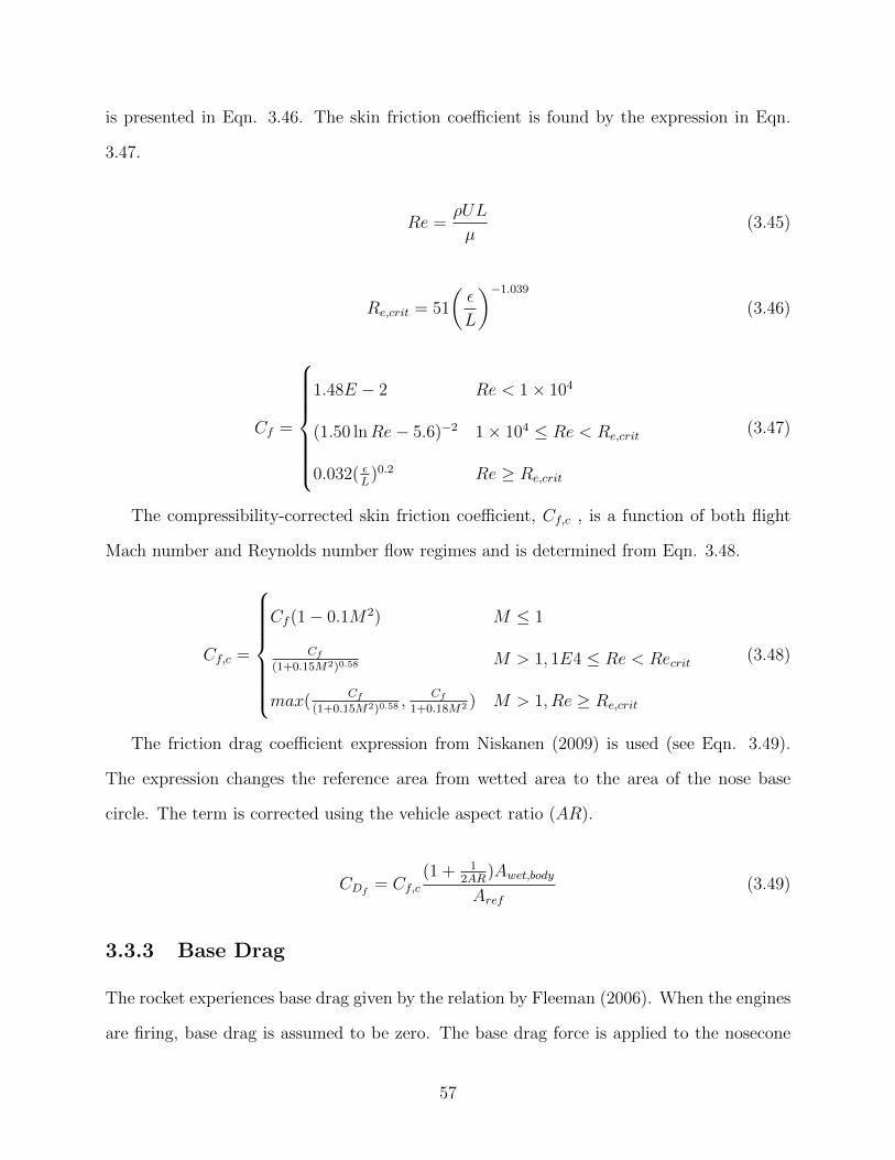
is presented in Eqn. 3.46. The skin friction coefficient is found by the expression in Eqn.

3.47.

Re =ρUL

µ(3.45)

Re,crit = 51

(ε

L

)−1.039

(3.46)

Cf =

1.48E − 2 Re < 1× 104

(1.50 lnRe− 5.6)−2 1× 104 ≤ Re < Re,crit

0.032( εL

)0.2 Re ≥ Re,crit

(3.47)

The compressibility-corrected skin friction coefficient, Cf,c , is a function of both flight

Mach number and Reynolds number flow regimes and is determined from Eqn. 3.48.

Cf,c =

Cf (1− 0.1M2) M ≤ 1

Cf(1+0.15M2)0.58

M > 1, 1E4 ≤ Re < Recrit

max(Cf

(1+0.15M2)0.58,

Cf1+0.18M2 ) M > 1, Re ≥ Re,crit

(3.48)

The friction drag coefficient expression from Niskanen (2009) is used (see Eqn. 3.49).

The expression changes the reference area from wetted area to the area of the nose base

circle. The term is corrected using the vehicle aspect ratio (AR).

CDf = Cf,c(1 + 1

2AR)Awet,body

Aref(3.49)

3.3.3 Base Drag

The rocket experiences base drag given by the relation by Fleeman (2006). When the engines

are firing, base drag is assumed to be zero. The base drag force is applied to the nosecone

57

element since the nosecone has the projected area necessary to transmit the drag force. Using

this relation, the calculated base drag agrees with Datcom, as will be seen in the verification

section.

CDbase = 0.12 + 0.13M2,M ≤ 1 (3.50)

CDbase = 0.25/M,M > 1 (3.51)

3.3.4 Cylindrical Section Normal Force

The cylindrical body CNα method is adapted from the method of Galejs (2018) (Eqn. 3.52).

The method needed to be linearized in the region of application, to determine the response

to small angles of attack away from the zero angle of attack reference point (otherwise CN

will be zero). A linear relationship is assumed between 0 and 0.025 radians, or approxi-

mately 1.4 degrees. The linearized relation is also corrected for compressibility using the

Prandtl–Glauert transformation presented by Niskanen (2009) (Eqns. 3.52 and 3.54). To

remedy the singularity in Eqn. 3.53, if the flight Mach number M is between 0.8 and 1.2,

the value of 0.8 is used. A value of 1.05 for K in Eqn. 3.52 and a minimum value of α of

0.025 radians to linearize CN leads to a good agreement with subsonic/transonic values for

nose/cylinder combinations from Messerchmitt-Boelkow-Blohm (1970) in Datcom. Beyond

Mach 2.0 the cylindrical body contribution is small compared to the nose.

CNα,M=0= 2K

AplanAref

α (3.52)

CNα =CNα,M=0

β(3.53)

β =√|1−M2| (3.54)

58

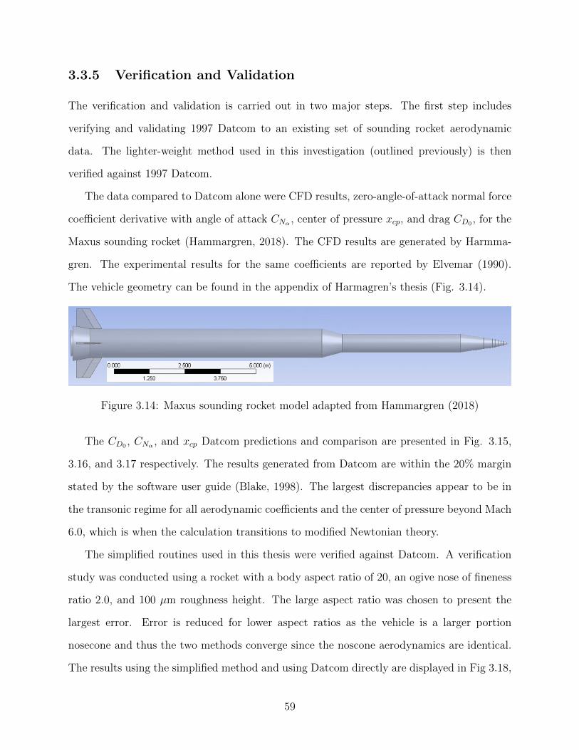
3.3.5 Verification and Validation

The verification and validation is carried out in two major steps. The first step includes

verifying and validating 1997 Datcom to an existing set of sounding rocket aerodynamic

data. The lighter-weight method used in this investigation (outlined previously) is then

verified against 1997 Datcom.

The data compared to Datcom alone were CFD results, zero-angle-of-attack normal force

coefficient derivative with angle of attack CNα , center of pressure xcp, and drag CD0 , for the

Maxus sounding rocket (Hammargren, 2018). The CFD results are generated by Harmma-

gren. The experimental results for the same coefficients are reported by Elvemar (1990).

The vehicle geometry can be found in the appendix of Harmagren’s thesis (Fig. 3.14).

Figure 3.14: Maxus sounding rocket model adapted from Hammargren (2018)

The CD0 , CNα , and xcp Datcom predictions and comparison are presented in Fig. 3.15,

3.16, and 3.17 respectively. The results generated from Datcom are within the 20% margin

stated by the software user guide (Blake, 1998). The largest discrepancies appear to be in

the transonic regime for all aerodynamic coefficients and the center of pressure beyond Mach

6.0, which is when the calculation transitions to modified Newtonian theory.

The simplified routines used in this thesis were verified against Datcom. A verification

study was conducted using a rocket with a body aspect ratio of 20, an ogive nose of fineness

ratio 2.0, and 100 µm roughness height. The large aspect ratio was chosen to present the

largest error. Error is reduced for lower aspect ratios as the vehicle is a larger portion

nosecone and thus the two methods converge since the noscone aerodynamics are identical.

The results using the simplified method and using Datcom directly are displayed in Fig 3.18,

59

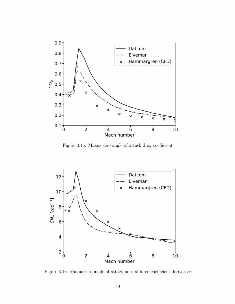
0 2 4 6 8 10Mach number

0.1

0.2

0.3

0.4

0.5

0.6

0.7

0.8

0.9CD

0DatcomElvemarHammargren (CFD)

Figure 3.15: Maxus zero angle of attack drag coefficient

0 2 4 6 8 10Mach number

2

4

6

8

10

12

CN [r

ad1 ]

DatcomElvemarHammargren (CFD)

Figure 3.16: Maxus zero angle of attack normal force coefficient derivative

60

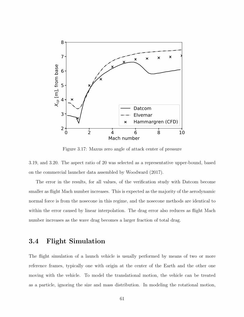
0 2 4 6 8 10Mach number

2

3

4

5

6

7

8

X cp [

m],

from

bas

e

DatcomElvemarHammargren (CFD)

Figure 3.17: Maxus zero angle of attack center of pressure

3.19, and 3.20. The aspect ratio of 20 was selected as a representative upper-bound, based

on the commercial launcher data assembled by Woodward (2017).

The error in the results, for all values, of the verification study with Datcom become

smaller as flight Mach number increases. This is expected as the majority of the aerodynamic

normal force is from the nosecone in this regime, and the nosecone methods are identical to

within the error caused by linear interpolation. The drag error also reduces as flight Mach

number increases as the wave drag becomes a larger fraction of total drag.

3.4 Flight Simulation

The flight simulation of a launch vehicle is usually performed by means of two or more

reference frames, typically one with origin at the center of the Earth and the other one

moving with the vehicle. To model the translational motion, the vehicle can be treated

as a particle, ignoring the size and mass distribution. In modeling the rotational motion,

61

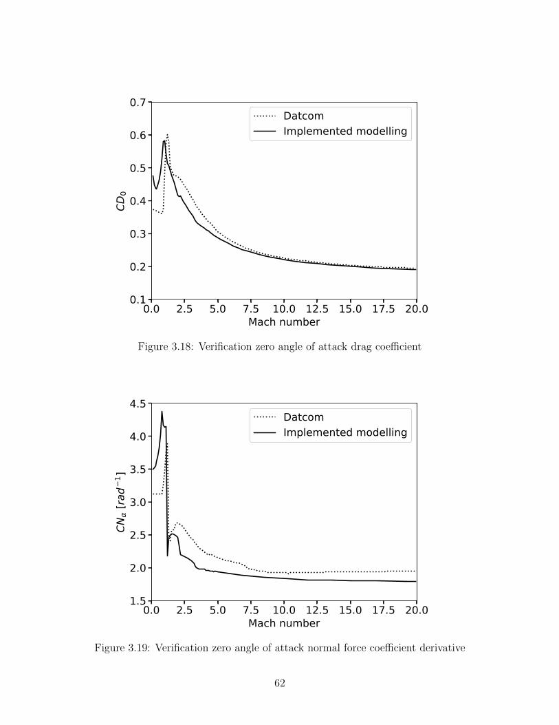
0.0 2.5 5.0 7.5 10.0 12.5 15.0 17.5 20.0Mach number

0.1

0.2

0.3

0.4

0.5

0.6

0.7CD

0DatcomImplemented modelling

Figure 3.18: Verification zero angle of attack drag coefficient

0.0 2.5 5.0 7.5 10.0 12.5 15.0 17.5 20.0Mach number

1.5

2.0

2.5

3.0

3.5

4.0

4.5

CN [r

ad1 ]

DatcomImplemented modelling

Figure 3.19: Verification zero angle of attack normal force coefficient derivative

62

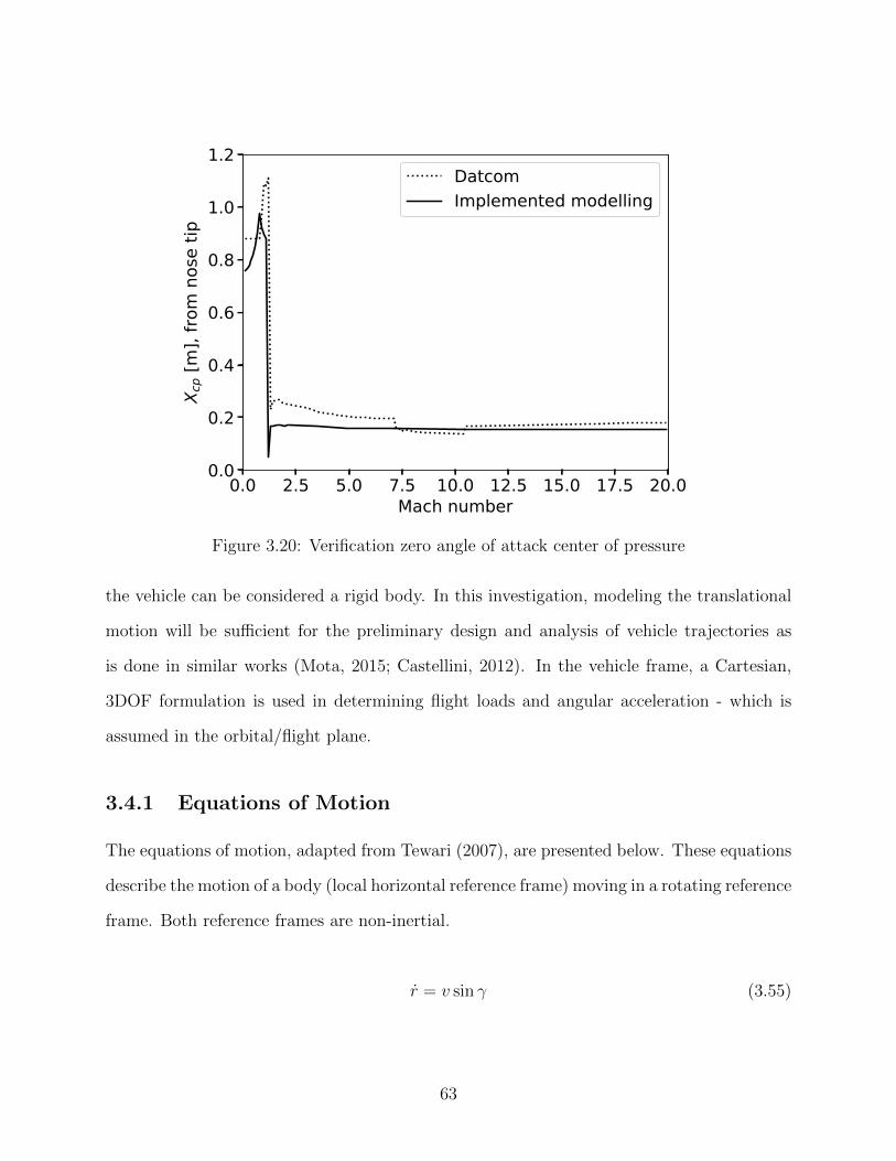
0.0 2.5 5.0 7.5 10.0 12.5 15.0 17.5 20.0Mach number

0.0

0.2

0.4

0.6

0.8

1.0

1.2

X cp [

m],

from

nos

e tip

DatcomImplemented modelling

Figure 3.20: Verification zero angle of attack center of pressure

the vehicle can be considered a rigid body. In this investigation, modeling the translational

motion will be sufficient for the preliminary design and analysis of vehicle trajectories as

is done in similar works (Mota, 2015; Castellini, 2012). In the vehicle frame, a Cartesian,

3DOF formulation is used in determining flight loads and angular acceleration - which is

assumed in the orbital/flight plane.

3.4.1 Equations of Motion

The equations of motion, adapted from Tewari (2007), are presented below. These equations

describe the motion of a body (local horizontal reference frame) moving in a rotating reference

frame. Both reference frames are non-inertial.

r = v sin γ (3.55)

63

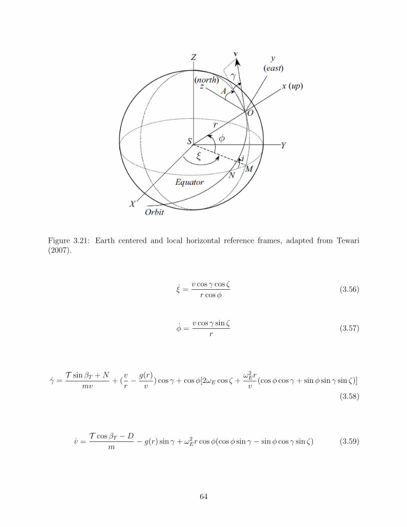
Figure 3.21: Earth centered and local horizontal reference frames, adapted from Tewari(2007).

ξ =v cos γ cos ζ

r cosφ(3.56)

φ =v cos γ sin ζ

r(3.57)

γ =T sin βT +N

mv+ (

v

r− g(r)

v) cos γ + cosφ[2ωE cos ζ +

ω2Er

v(cosφ cos γ + sinφ sin γ sin ζ)]

(3.58)

v =T cos βT −D

m− g(r) sin γ + ω2

Er cosφ(cosφ sin γ − sinφ cos γ sin ζ) (3.59)

64

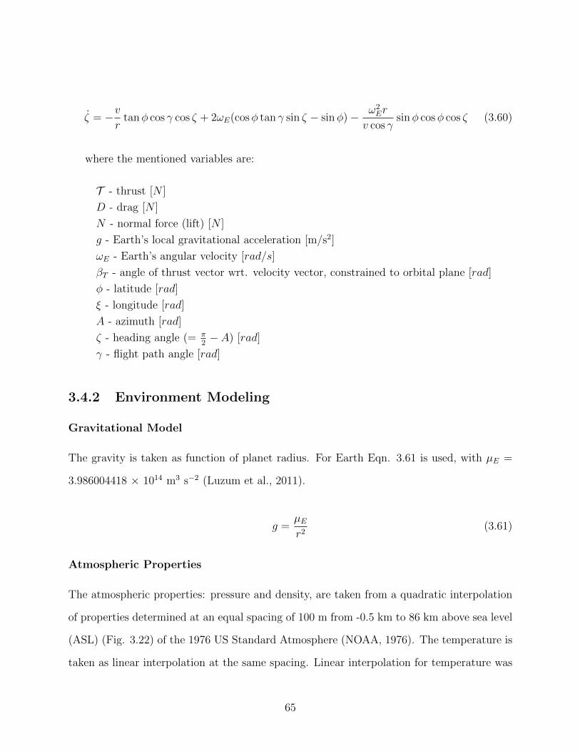
ζ = −vr

tanφ cos γ cos ζ + 2ωE(cosφ tan γ sin ζ − sinφ)− ω2Er

v cos γsinφ cosφ cos ζ (3.60)

where the mentioned variables are:

T - thrust [N ]

D - drag [N ]

N - normal force (lift) [N ]

g - Earth’s local gravitational acceleration [m/s2]

ωE - Earth’s angular velocity [rad/s]

βT - angle of thrust vector wrt. velocity vector, constrained to orbital plane [rad]

φ - latitude [rad]

ξ - longitude [rad]

A - azimuth [rad]

ζ - heading angle (= π2− A) [rad]

γ - flight path angle [rad]

3.4.2 Environment Modeling

Gravitational Model

The gravity is taken as function of planet radius. For Earth Eqn. 3.61 is used, with µE =

3.986004418 × 1014 m3 s−2 (Luzum et al., 2011).

g =µEr2

(3.61)

Atmospheric Properties

The atmospheric properties: pressure and density, are taken from a quadratic interpolation

of properties determined at an equal spacing of 100 m from -0.5 km to 86 km above sea level

(ASL) (Fig. 3.22) of the 1976 US Standard Atmosphere (NOAA, 1976). The temperature is

taken as linear interpolation at the same spacing. Linear interpolation for temperature was

65

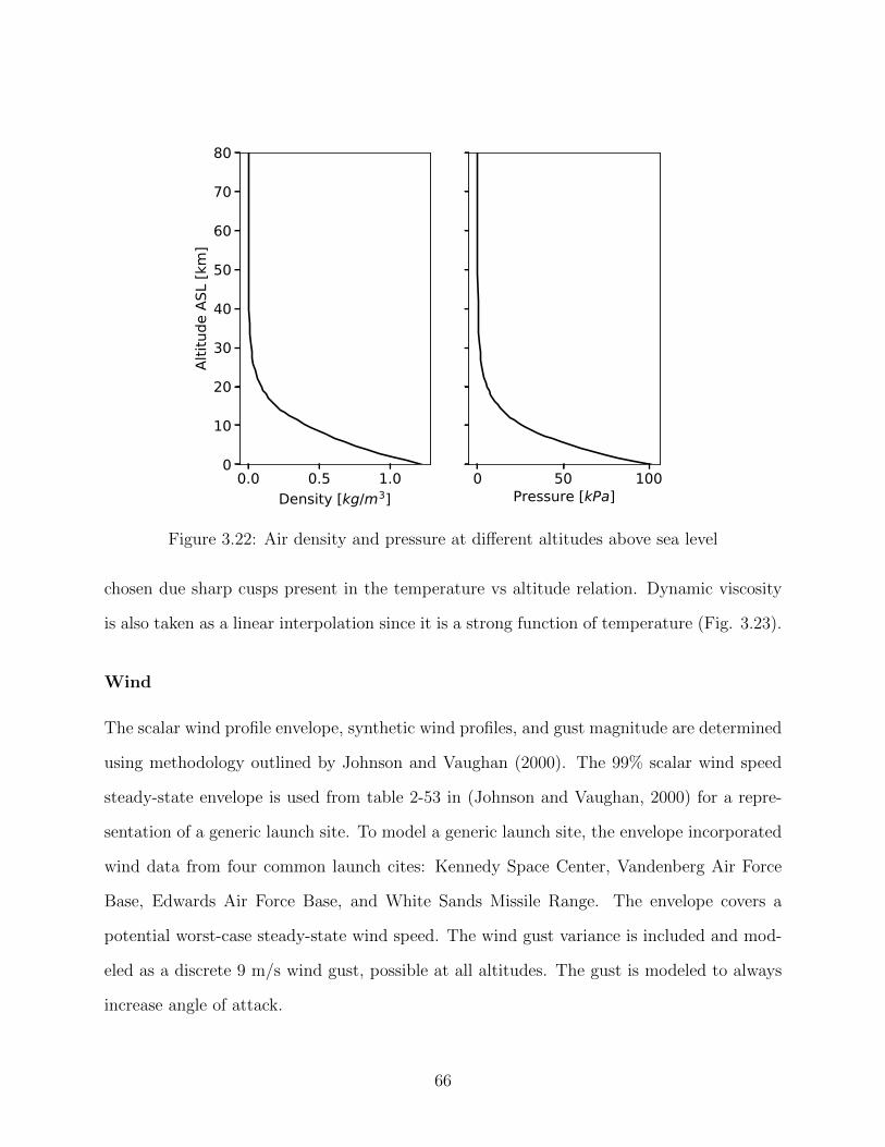
0.0 0.5 1.0Density [kg/m3]

0

10

20

30

40

50

60

70

80

Altit

ude

ASL

[km

]

0 50 100Pressure [kPa]

Figure 3.22: Air density and pressure at different altitudes above sea level

chosen due sharp cusps present in the temperature vs altitude relation. Dynamic viscosity

is also taken as a linear interpolation since it is a strong function of temperature (Fig. 3.23).

Wind

The scalar wind profile envelope, synthetic wind profiles, and gust magnitude are determined

using methodology outlined by Johnson and Vaughan (2000). The 99% scalar wind speed

steady-state envelope is used from table 2-53 in (Johnson and Vaughan, 2000) for a repre-

sentation of a generic launch site. To model a generic launch site, the envelope incorporated

wind data from four common launch cites: Kennedy Space Center, Vandenberg Air Force

Base, Edwards Air Force Base, and White Sands Missile Range. The envelope covers a

potential worst-case steady-state wind speed. The wind gust variance is included and mod-

eled as a discrete 9 m/s wind gust, possible at all altitudes. The gust is modeled to always

increase angle of attack.

66

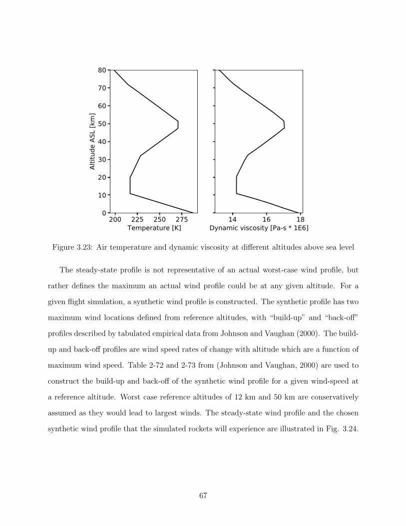
200 225 250 275Temperature [K]

0

10

20

30

40

50

60

70

80

Altit

ude

ASL

[km

]

14 16 18Dynamic viscosity [Pa-s * 1E6]

Figure 3.23: Air temperature and dynamic viscosity at different altitudes above sea level

The steady-state profile is not representative of an actual worst-case wind profile, but

rather defines the maximum an actual wind profile could be at any given altitude. For a

given flight simulation, a synthetic wind profile is constructed. The synthetic profile has two

maximum wind locations defined from reference altitudes, with “build-up” and “back-off”

profiles described by tabulated empirical data from Johnson and Vaughan (2000). The build-

up and back-off profiles are wind speed rates of change with altitude which are a function of

maximum wind speed. Table 2-72 and 2-73 from (Johnson and Vaughan, 2000) are used to

construct the build-up and back-off of the synthetic wind profile for a given wind-speed at

a reference altitude. Worst case reference altitudes of 12 km and 50 km are conservatively

assumed as they would lead to largest winds. The steady-state wind profile and the chosen

synthetic wind profile that the simulated rockets will experience are illustrated in Fig. 3.24.

67

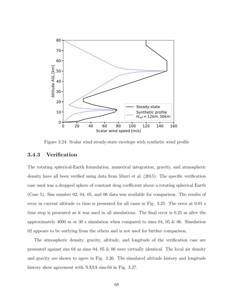
0 20 40 60 80 100 120 140 160Scalar wind speed [m/s]

0

10

20

30

40

50

60

70

80

Altit

ude

ASL

[km

]

Steady-stateSynthetic profileHref = 12km, 50km

Figure 3.24: Scalar wind steady-state envelope with synthetic wind profile

3.4.3 Verification

The rotating spherical-Earth formulation, numerical integration, gravity, and atmospheric

density have all been verified using data from Murri et al. (2015). The specific verification

case used was a dropped sphere of constant drag coefficient above a rotating spherical Earth

(Case 5). Sim number 02, 04, 05, and 06 data was available for comparison. The results of

error in current altitude vs time is presented for all cases in Fig. 3.25. The error at 0.01 s

time step is presented as it was used in all simulations. The final error is 0.25 m after the

approximately 4000 m or 30 s simulation when compared to sims 04, 05 & 06. Simulation

02 appears to be outlying from the others and is not used for further comparison.

The atmospheric density, gravity, altitude, and longitude of the verification case are

presented against sim 04 as sims 04, 05 & 06 were virtually identical. The local air density

and gravity are shown to agree in Fig. 3.26. The simulated altitude history and longitude

history show agreement with NASA sim-04 in Fig. 3.27.

68

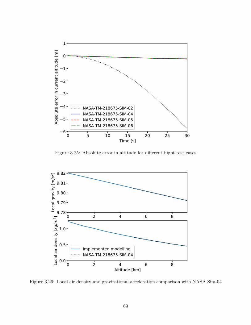
0 5 10 15 20 25 30Time [s]

6

5

4

3

2

1

0

1

Abso

lute

erro

r in

curre

nt a

ltitu

de [m

]

NASA-TM-218675-SIM-02NASA-TM-218675-SIM-04NASA-TM-218675-SIM-05NASA-TM-218675-SIM-06

Figure 3.25: Absolute error in altitude for different flight test cases

0 2 4 6 89.78

9.79

9.80

9.81

9.82

Loca

l gra

vity

[m/s

2 ]

0 2 4 6 8Altitude [km]

0.0

0.5

1.0

Loca

l air

dens

ity [k

g/m

3 ]

Implemented modellingNASA-TM-218675-SIM-04

Figure 3.26: Local air density and gravitational acceleration comparison with NASA Sim-04

69

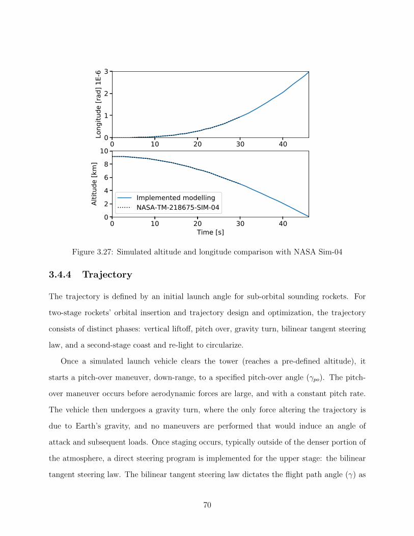
0 10 20 30 400

1

2

3

Long

itude

[rad

] 1E-

6

0 10 20 30 40Time [s]

02468

10

Altit

ude

[km

]

Implemented modellingNASA-TM-218675-SIM-04

Figure 3.27: Simulated altitude and longitude comparison with NASA Sim-04

3.4.4 Trajectory

The trajectory is defined by an initial launch angle for sub-orbital sounding rockets. For

two-stage rockets’ orbital insertion and trajectory design and optimization, the trajectory

consists of distinct phases: vertical liftoff, pitch over, gravity turn, bilinear tangent steering

law, and a second-stage coast and re-light to circularize.

Once a simulated launch vehicle clears the tower (reaches a pre-defined altitude), it

starts a pitch-over maneuver, down-range, to a specified pitch-over angle (γpo). The pitch-

over maneuver occurs before aerodynamic forces are large, and with a constant pitch rate.

The vehicle then undergoes a gravity turn, where the only force altering the trajectory is

due to Earth’s gravity, and no maneuvers are performed that would induce an angle of

attack and subsequent loads. Once staging occurs, typically outside of the denser portion of

the atmosphere, a direct steering program is implemented for the upper stage: the bilinear

tangent steering law. The bilinear tangent steering law dictates the flight path angle (γ) as

70

a function of time into the burn and can be found from Eqn. 3.62, adapted from Castellini

(2012). The The flight path heading rate of change can also be determined at this stage and

used as set points for a controller. The controller would apply torques to the vehicle to impart

angular acceleration/velocity either using gas thrusters or TVC. Defining the flight path

heading at time into the flight, or burn, with some tune-able parameters or control points

is done in most works surveyed (Castellini, 2012; Mota, 2015; Miranda, 2015; Woodward,

2017). The control system for controlling flight path heading (i.e solving equations of motion

in vehicle frame with lateral thrust imparting error corrections) was neglected in this thesis

to increase computational speed, Castellini (2012) found that very small steering losses were

found when including the upper stage steering control into the simulation. Neglecting the

steering control modeling is typically done in other works (Miranda, 2015; Woodward, 2017).

Steering is however incorporated into the simulation of the first stage ascent to determine

loads and first stage steering losses.

γ =

tan−1

(cχ tan γi+(tan γf−cχ tan γi)

τbb

cχ+(1−cχ)τbb

)0 ≤ τb ≤ b

γf τb > b

(3.62)

where,

γ - flight path angle [rad]

γi - initial flight path angle at beginning of control [rad]

γf - final flight path angle (typically 0, tangent to Earth’s surface) [rad]

c - fitting parameter to control trajectory shape, 10 ≤ c ≤ 100

χ - fitting parameter exponent to control trajectory shape, -1.0 ≤ χ ≤ 1.0

τb - normalized burn time, 0.0 ≤ τb ≤ 1.0

b - normalized burn time truncation parameter, 0 < b ≤ 1.0

The current flight path angle (γ), in the flight path plane, is controlled to match that

defined by Eqn. 3.62 at each instant of the burn time. The parameter τb is the normalized

burn time, c and χ are constants defining the shape of the trajectory. The γi and γf variables

are the initial and final flight path angles respectively. The initial flight path angle of the

71

second stage is determined by the flight profile of the first stage. The final flight path angle

is 0 rad (tangent to the Earth’s surface).

During the first stage burn, before Second-Engine Cut-off, number one (SECO-1), the

resulting orbit (if the engine was to be cut-off) is continuously calculated at each time

step. When the calculated orbit apogee reaches the target apogee at the current altitude

(perigee), the burn is truncated. The Python module orbitalpy (McLean, 2020) is used to

calculate the orbital elements from the state vector (position and velocity in 3D space). The

six arguments of a position and velocity vector are translated into six Keplerian elements

that define the orbit geometry in space (Vallado, 2010) where the apogee and perigee can be

extracted. The initial orbit at SECO-1 is elliptical, the final circular orbit is accomplished by

a circularization burn on the opposite side of the Earth. However, the actual time marching

does not persist around the Earth in the simulation to increase computational speed. The

required propellant mass at the average remaining deliverable Isp is calculated using the

rocket equation (Eqn. 3.1) since the equation’s assumptions are valid in this case. An

impulsive-thrust orbit transfer is assumed for the in-orbit revenuers which is valid for typical

chemical rockets since the burn times are small fractions of total orbit times (Vallado, 2010).

The required propellant is checked with the available propellant mass. The ∆V residual is

converged to zero in the global optimizer. The ∆V residual is also allowed to go negative

and be converged to zero or positive by the global optimizer to provide a better gradient in

the solution space.

Trajectory Optimization and Convergence

The required position (radius) and velocity vector of the vehicle in an inertial reference

frame, at SECO-1, is prescribed by the desired orbit (Vallado, 2010). The trajectory design

consists of two parts: meeting required orbit parameters and minimizing the propellant

usage. The trajectory design is multi-objective and consists of solving a boundary-value

problem, where the trajectory parameters are adjusted such that the final solution matches

72

that desired, while also minimizing propellant usage. The trajectory design and optimization

is accomplished through numerous flight simulations. If the trajectory design was to be

coupled with the structural design the number of required flight simulations would greatly

increase. The trajectory was desired to be decoupled from the structural analysis of the

vehicle to reduce the run time of complete design iterations. The solution decouples the

trajectory designs of the stages. The first-stage ascent trajectory is completely defined by

a pitch-over/gravity turn (γpo), the structures can be converged to their optimal values,

through least squares, including the upper stage since maximum loading occurs during first-

stage ascent. The structures of the upper stage are then assumed independent of the upper

stage trajectory, which is a reasonable assumption as staging is typically done near negligible

dynamic pressure. A more detailed description of the structural design is completed in the

structural design section. The upper stage trajectory flight segment can then be optimized,

at a local level, by altering the available parameters that define its trajectory (c, χ, and b).

The cost function that was used to optimize upper stage trajectories is the error of the

SECO-1 altitude from the target, minus the ∆V of the remaining propellant residual on

board after circularization. The optimizer seeks to minimize the cost function. The ∆V

is calculated using Eqn. 3.1, the remaining average vacuum specific impulse, and known

remaining propellant and inert masses.

The algorithm that was found to quickly and reliably converge on optimal upper stage

trajectories is the L-BFGS-B algorithm in the Scipy Optimize module minimize function

(Virtanen et al., 2020). The L-BFGS-B algorithm is chosen as this problem is non-linear.

The limited memory (L-), bounded (-B) BFGS algorithm is in the class of quasi-Newton’s

method and is found to quickly converge to optimal trajectory parameters compared to other

non-linear methods available in the Optimize module. The good performance is attributed

to the smoothness of the objective function, and short bounds on the parameters. The

algorithm has a narrow search space and only three dimensions and finds optimal solutions

reliably and quickly.

73

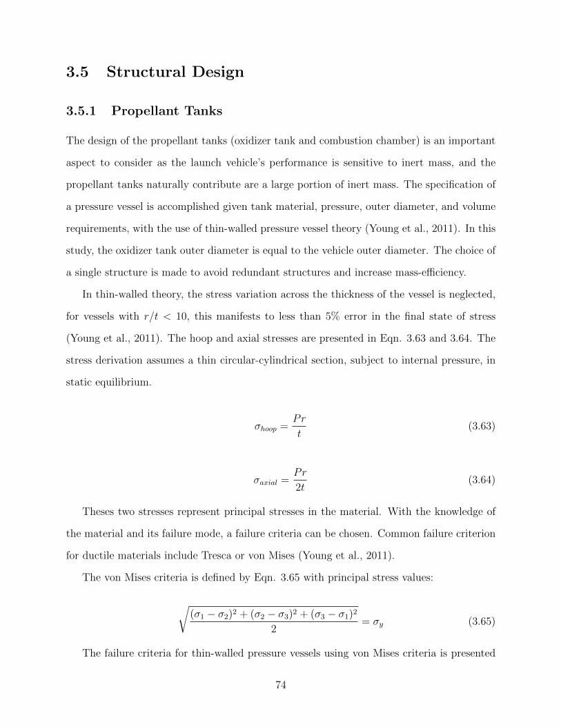
3.5 Structural Design

3.5.1 Propellant Tanks

The design of the propellant tanks (oxidizer tank and combustion chamber) is an important

aspect to consider as the launch vehicle’s performance is sensitive to inert mass, and the

propellant tanks naturally contribute are a large portion of inert mass. The specification of

a pressure vessel is accomplished given tank material, pressure, outer diameter, and volume

requirements, with the use of thin-walled pressure vessel theory (Young et al., 2011). In this

study, the oxidizer tank outer diameter is equal to the vehicle outer diameter. The choice of

a single structure is made to avoid redundant structures and increase mass-efficiency.

In thin-walled theory, the stress variation across the thickness of the vessel is neglected,

for vessels with r/t < 10, this manifests to less than 5% error in the final state of stress

(Young et al., 2011). The hoop and axial stresses are presented in Eqn. 3.63 and 3.64. The

stress derivation assumes a thin circular-cylindrical section, subject to internal pressure, in

static equilibrium.

σhoop =Pr

t(3.63)

σaxial =Pr

2t(3.64)

Theses two stresses represent principal stresses in the material. With the knowledge of

the material and its failure mode, a failure criteria can be chosen. Common failure criterion

for ductile materials include Tresca or von Mises (Young et al., 2011).

The von Mises criteria is defined by Eqn. 3.65 with principal stress values:

√(σ1 − σ2)2 + (σ2 − σ3)2 + (σ3 − σ1)2

2= σy (3.65)

The failure criteria for thin-walled pressure vessels using von Mises criteria is presented

74

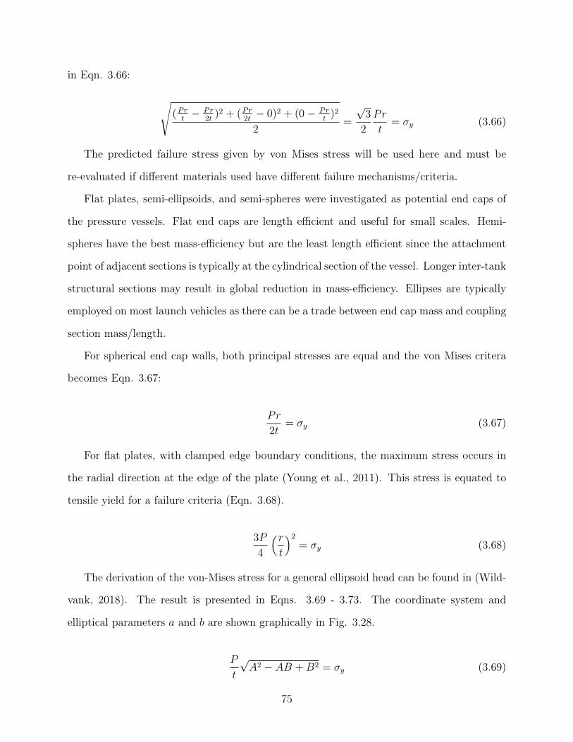
in Eqn. 3.66:

√(Prt− Pr

2t)2 + (Pr

2t− 0)2 + (0− Pr

t)2

2=

√3

2

Pr

t= σy (3.66)

The predicted failure stress given by von Mises stress will be used here and must be

re-evaluated if different materials used have different failure mechanisms/criteria.

Flat plates, semi-ellipsoids, and semi-spheres were investigated as potential end caps of

the pressure vessels. Flat end caps are length efficient and useful for small scales. Hemi-

spheres have the best mass-efficiency but are the least length efficient since the attachment

point of adjacent sections is typically at the cylindrical section of the vessel. Longer inter-tank

structural sections may result in global reduction in mass-efficiency. Ellipses are typically

employed on most launch vehicles as there can be a trade between end cap mass and coupling

section mass/length.

For spherical end cap walls, both principal stresses are equal and the von Mises critera

becomes Eqn. 3.67:

Pr

2t= σy (3.67)

For flat plates, with clamped edge boundary conditions, the maximum stress occurs in

the radial direction at the edge of the plate (Young et al., 2011). This stress is equated to

tensile yield for a failure criteria (Eqn. 3.68).

3P

4

(rt

)2

= σy (3.68)

The derivation of the von-Mises stress for a general ellipsoid head can be found in (Wild-

vank, 2018). The result is presented in Eqns. 3.69 - 3.73. The coordinate system and

elliptical parameters a and b are shown graphically in Fig. 3.28.

P

t

√A2 − AB +B2 = σy (3.69)

75

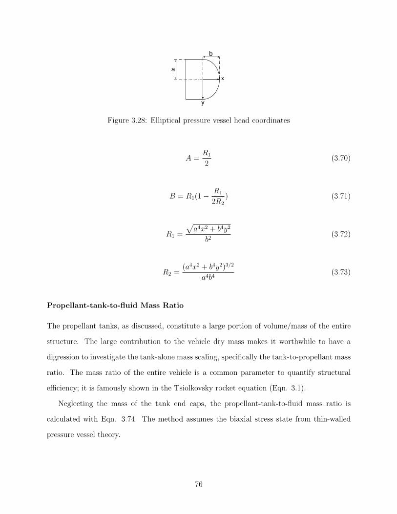
y

xa

b

Figure 3.28: Elliptical pressure vessel head coordinates

A =R1

2(3.70)

B = R1(1− R1

2R2

) (3.71)

R1 =

√a4x2 + b4y2

b2(3.72)

R2 =(a4x2 + b4y2)3/2

a4b4(3.73)

Propellant-tank-to-fluid Mass Ratio

The propellant tanks, as discussed, constitute a large portion of volume/mass of the entire

structure. The large contribution to the vehicle dry mass makes it worthwhile to have a

digression to investigate the tank-alone mass scaling, specifically the tank-to-propellant mass

ratio. The mass ratio of the entire vehicle is a common parameter to quantify structural

efficiency; it is famously shown in the Tsiolkovsky rocket equation (Eqn. 3.1).

Neglecting the mass of the tank end caps, the propellant-tank-to-fluid mass ratio is

calculated with Eqn. 3.74. The method assumes the biaxial stress state from thin-walled

pressure vessel theory.

76

mfluid

mtank

=ρfluid–Vfluid

ρtank,material–Vtank,material≈ ρfluidπr

2L

ρmaterial2πrtL=

ρfluidπr2L

ρmaterial√

3πr Prσallow

L=

ρfluidσallow√3ρmaterialP

(3.74)

Equation 3.74 shows, with the previously stated assumptions, that the mass ratio can only

be altered by the density of the fluid contained, the pressure it’s stored at, and the strength-

to-weight ratio of tank material. The propellant-to-tank mass ratio is not a function of

geometry (scale).

The theoretical scaling mass ratio is compared to a design of a spherical-capped oxidizer

tank for different internal volumes. The vessel outer diameter was 1.0 m and the volume was

ranged from 0.6 m3 to 80 m3. The internal pressure and fluid density was 300 kPa and 1000

kg/m3 respectively. The material density and allowable stress was 2700 kg/m3 and 120 MPa

respectively. The design and theoretical scaling mass ratios are presented in Fig. 3.29. The

minor discrepancy observed, at the largest aspect ratios, is attributed to assuming the tank

cross-sectional area is the circumference multiplied by thickness in the theoretical scaling

estimate.

3.5.2 Combined Loading

In general, for a rocket cylindrical section considered here, loading can occur in the forms

of: axial force, bending moment, and internal pressure (Fig. 3.30). The vehicle weight, in

addition to thrust which is reacted by inertial loads, and drag, provide the net axial force

(Fax). The pure axial stress is expressed with the net axial force: σax = FaxA

. Bending loads

arise from lateral forces due to the vehicle response to angle of attack, lateral components of

body forces, and thrust vectoring. The maximum/minimum bending loads occur on opposite

sides of the neutral axis: σb = ±MrI

. The parameter I is the sectional area moment of inertia;

values are from Young et al. (2011). Variable A is cross-sectional area of the thin cylindrical

section. Stress from internal pressure are expressed by Eqns. 3.63 and 3.64.

77

0 20 40 60 80 100Tank aspect ratio [L/D]

84

86

88

90

92

94

96

98m

fluid

/mta

nk

Spherical-cappedEstimated theoretical scaling

Figure 3.29: Comparison of oxidizer tank design mass to theoretical scaling estimate

Figure 3.30: Axial, lateral, bending moment, and internal pressure loads on a generic rocketelement cylinder

78

The combined von-Mises stress can be calculated using Eqn. 3.65 for two 2-D stress

elements at the maximum and minimum bending stress locations. The first principal stress

is the sum of the axial, bending, and axial internal pressure stress (see Eqn. 3.75). The

second principal stress is the hoop stress due to internal pressure (Eqn. 3.76).

σ1 =FaxA± Mr

I+Pr

2t(3.75)

σ2 =Pr

t(3.76)

3.5.3 Buckling of Thin-walled Cylinders

This section will analyze all of the combined loads and link to buckling failure of thin cylin-

drical shells. The thin isotropic circular cylinder failure criterion under axial compression,

bending, and internal pressure is used from NASA TR-SP-8007 (Peterson et al., 1968).

Isotropic circular cylinders are assumed for each rocket component. Buckling and collapse

coincide for circular cylinders under both axial compression and bending (Peterson et al.,

1968).

The critical axial stress for a thin cylinder buckling failure is represented by Eqn. 3.77.

Note that respectively variables t and r are cylinder thickness and radius. E and µ are the

material Youngs Modulus and Poisson ratio. The variable γx is the empirical correlation fac-

tor to account for differences between the theory and predicted instability loads, specifically

for axial compression. The variable γx is determined from Eqns. 3.78 - 3.79:

σx,crit =(γx + ∆γ)E√

3(1− µ2)

t

r+Pr

2t(3.77)

where ∆γ ranges between 0.02 and 0.2, is a function of pressure, and is taken from figure 6

in (Peterson et al., 1968). As well, note the following:

79

γx = 1− 0.901(1− e−Φ) (3.78)

Φ =1

16

√r

t, (r

t) < 1500 (3.79)

Peterson et al. (1968) warn that predictions of critical load past length-radius ratios

greater than 5.0 have not been validated by experiments. Critical loads for bending are

given by a different correlation factor, γb, Eqn. 3.80. The bending correlation factor can

be used similarly in Eqn. 3.81 to obtain the critical maximum stress in bending. An 80 %

factor is applied to the collapse resistance theoretically supplied by internal pressure as per

NASA TR-SP-8007.

γb = 1− 0.731(1− e−Φ) (3.80)

σb,crit =(γb + ∆γ)E√

3(1− µ2)

t

r+ 0.8

Pr

t(3.81)

The interaction of the two stresses for predicting failure is given in Eqn. 3.82. The ratio,

Rx, is the ratio of the axial stress in a cylinder subjected to more than one type of loading to

the allowable stress in the cylinder subjected to only axial compression. Rb is ratio of stress

due to bending in the combined scenario to the allowable bending-alone stress.

Rx +Rb =σx

σx,allow+

σbσb,allow

≤ 1 (3.82)

3.5.4 Flight Loads

The axial and transverse loads that the rocket experiences in flight are generally caused by:

body forces (inertial and gravitational), aerodynamic forces (lift and drag), and thrust forces

(axial from the principal thrust delivery system, and transverse from thrust vector control

80

(TVC)). The considered loads are combined into resultants at element center of mass and

pressure. The forces are then decomposed into axial forces, lateral shear forces, and bending

moments at the element interfaces (nodes) along the axial length of the rocket.

At each instant in flight, the loads are calculated assuming the current wind is the

highest possible as outlined by the steady-state 99 % envelope, in the environmental modeling

section, in addition to a discrete sharp-edged gust. The first-stage engine(s) lateral thrust

from the available TVC is used to trim the vehicle against the aerodynamic loads, to create

a zero moment about the center of mass. The act of trimming can potentially create a

large bending stress on the vehicle. The additional gust is assumed to occur over a short

time and creates a worst-case dynamic response and loading situation for the vehicle. The

actual synthetic wind profile used in flight simulations is not the same one used to determine

maximum possible loads, and is defined in the environmental modeling section. The synthetic

profile is used mainly in quantifying the steering losses and effect of wind on the trajectory.

During the dynamic response, angular acceleration and lateral acceleration contribute

to inertial loads and relief, however aerodynamic plunge and pitch damping are neglected.

The axial, shear, and bending moment equations have been derived with the nosecone tip

as the origin. Bending moment, shear, and axial loads vanish at the free ends, if none are

prescribed there, and the successive loads can be determined by marching in space down the

length of the rocket vehicle.

The shear force, S, acting on the face of a rocket element can be determined using

Newton’s 2nd law in the lateral (y) direction (Eqn. 3.83):

Si+1 = Si +mi(ay − (xcg − xcg,i)d2γ

dt2) + qArefCNα,iα (3.83)

where q is the dynamic pressure.

The xcg is the axial location of the center of gravity, measured from the nosecone tip

(Eqn. 3.84). The subscript i denotes element quantities. Element center of mass/gravity

xcg,i is measured from the element front:

81

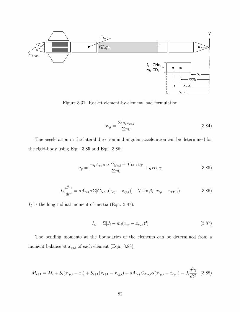
FThrust

FAero

FBody

xixcgi

xcpixi+1

CNαiCDimi

Ji

Figure 3.31: Rocket element-by-element load formulation

xcg =Σmixcg,i

Σmi

(3.84)

The acceleration in the lateral direction and angular acceleration can be determined for

the rigid-body using Eqn. 3.85 and Eqn. 3.86:

ay =−qArefαΣCNα,i + T sin βT

Σmi

+ g cos γ (3.85)

ILd2γ

dt2= qArefαΣ[CNα,i(xcg − xcp,i)]− T sin βT (xcg − xTV C) (3.86)

IL is the longitudinal moment of inertia (Eqn. 3.87):

IL = Σ[Ji +mi(xcg − xcg,i)2] (3.87)

The bending moments at the boundaries of the elements can be determined from a

moment balance at xcg,i of each element (Eqn. 3.88):

Mi+1 = Mi + Si(xcg,i − xi) + Si+1(xi+1 − xcg,i) + qArefCNα,iα(xcg,i − xcp,i)− Jid2γ

dt2(3.88)

82

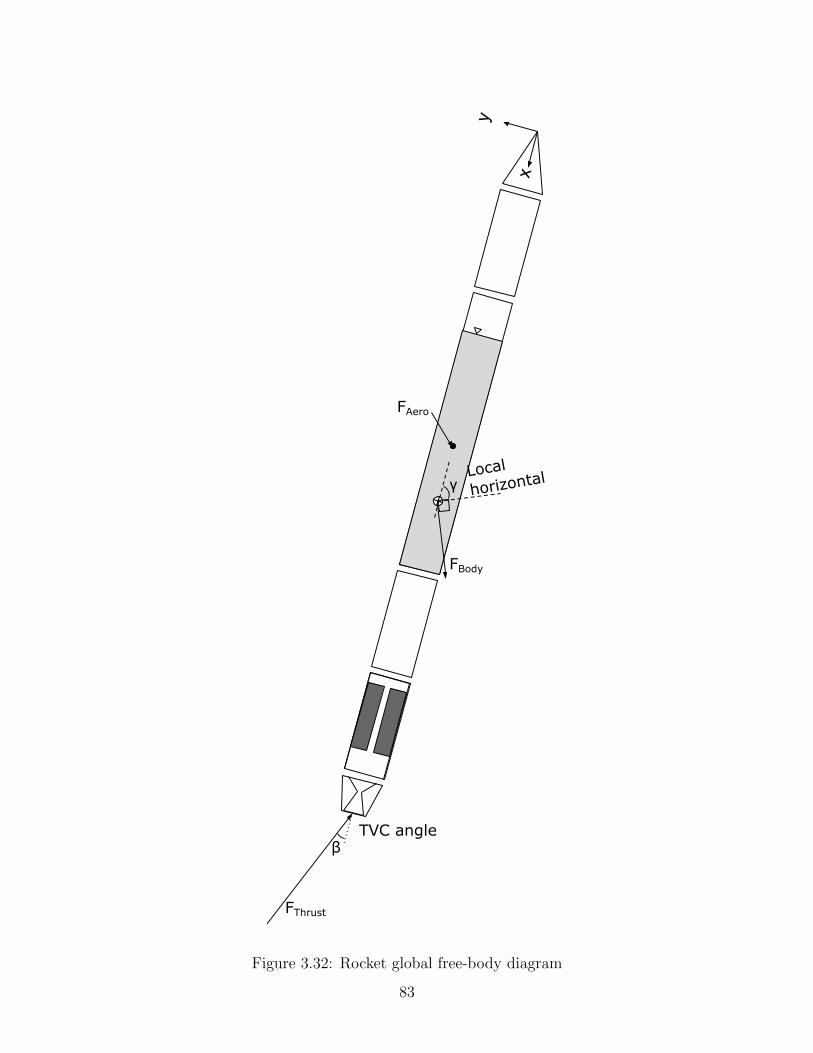
β

FThrust

FAero

FBody

Local

horizontal

TVC angle

γ

Figure 3.32: Rocket global free-body diagram

83

The axial loads can be determined from applying Newton’s 2nd law in the longitudinal

(x) direction (Eqn. 3.89):

Fi+1 = Fi +miax + qArefCD,i (3.89)

where ax is the longitudinal (x) acceleration (Eqn. 3.90):

ax =(T cos βT − qArefΣCDi)

Σmi

− g sin γ (3.90)

The boundary conditions are prescribed by Eqn. 3.91:

S0 = 0,M0 = 0, F0 = 0, Sn = T cos βT , Fn = T sin βT (3.91)

3.5.5 Special Load Cases

A few special load cases are added to size various elements:

� Loss of pressure on-pad

The load case of a depressurized vehicle on the pad is analyzed. This is employed after

realizing that the optimizer was exploiting pressure-stabilized structures that could

not support their own weight if pressure was lost. All masses onboard are the starting

values (full propellant loading, worst case), but all propellant tanks have zero pressure.

This load case ensures the buckling margins of the oxidizer tanks are sufficient for a

zero thrust, on-pad case. The loss of pressure in-flight may have insufficient margins

if thrust can still occur when the tanks are not pressurized.

� Aft engine section skirt axial compression from vehicle weight on-pad

This load case checks the aft section around the main engines while bearing the total

vehicle weight in compression, statically on the launch pad. This is in addition to all

flight loads.

84

� Upper stage flight loads

The lateral loads on the second stage are neglected during the flight of the second

stage. It is assumed that all contributing factors to lateral loads are small for the upper

stage’s flight. The upper stage’s lateral loads are still calculated during the first-stage

ascent, when both stages are connected. This assumption requires validation once the

full mission simulation is performed or can be maintained with a minimum staging

altitude constraint. The assumption of negligible lateral loads results in being able to

determine the upper stage flight loads outside of the upper stage flight loop, which

drastically reduces computational time. The maximum axial loads and maximum fluid

static pressure are calculated for upper stages assuming zero back pressure for the

propulsion system, and aligned velocity and gravity vectors (worst case).

3.5.6 Modal Analysis

The displacement/stiffness constraints are another important aspect of the launch vehicle’s

structural design. The stiffness requirements are based on a modal (frequency domain) anal-

ysis of a finite-beam-element model of a rocket. The rocket model is divided into discrete

elements, the same elements as previously discussed, each with geometric, mass, and mate-

rial properties. The stiffness constraints are the lowest allowable bending and axial mode

fundamental vibrational frequencies. The fundamental modes increase in frequency value as

overall rigidity is increased. The values of lower bounds are 25 Hz and 10 Hz for axial and

bending modes respectively, taken from launch vehicle design criteria and based on previous

existing launchers from Larson and Wetrz (1999). The rigidity constraints are important

for maintaining control stability and avoiding any aeroelastic instabilities, that could lead

to high fatigue loading or divergence.

In the modal analysis formulation, each rocket element is modeled as a cylinder with

uniform mass distribution. The mass and stiffness matrices are determined for each element

based on Bernoulli-Euler beam theory (Gavin, 2018). A single element mass matrix and

85

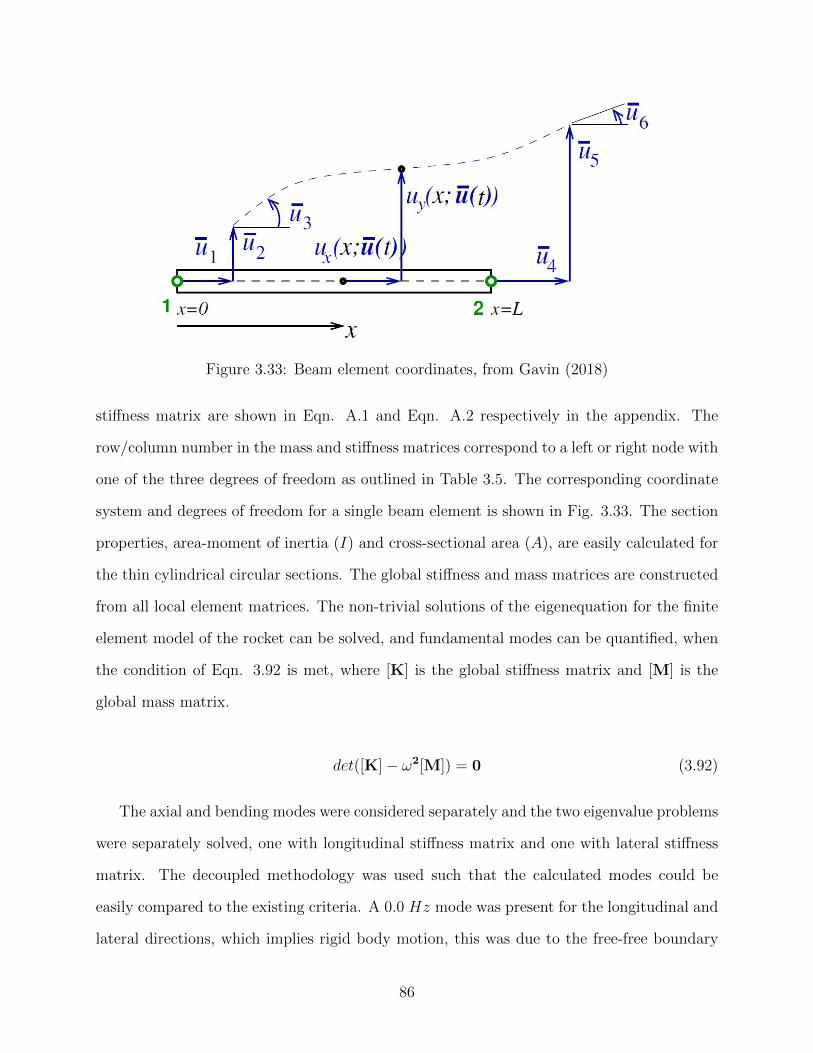
Figure 3.33: Beam element coordinates, from Gavin (2018)

stiffness matrix are shown in Eqn. A.1 and Eqn. A.2 respectively in the appendix. The

row/column number in the mass and stiffness matrices correspond to a left or right node with

one of the three degrees of freedom as outlined in Table 3.5. The corresponding coordinate

system and degrees of freedom for a single beam element is shown in Fig. 3.33. The section

properties, area-moment of inertia (I) and cross-sectional area (A), are easily calculated for

the thin cylindrical circular sections. The global stiffness and mass matrices are constructed

from all local element matrices. The non-trivial solutions of the eigenequation for the finite

element model of the rocket can be solved, and fundamental modes can be quantified, when

the condition of Eqn. 3.92 is met, where [K] is the global stiffness matrix and [M] is the

global mass matrix.

det([K]− ω2[M]) = 0 (3.92)

The axial and bending modes were considered separately and the two eigenvalue problems

were separately solved, one with longitudinal stiffness matrix and one with lateral stiffness

matrix. The decoupled methodology was used such that the calculated modes could be

easily compared to the existing criteria. A 0.0 Hz mode was present for the longitudinal and

lateral directions, which implies rigid body motion, this was due to the free-free boundary

86

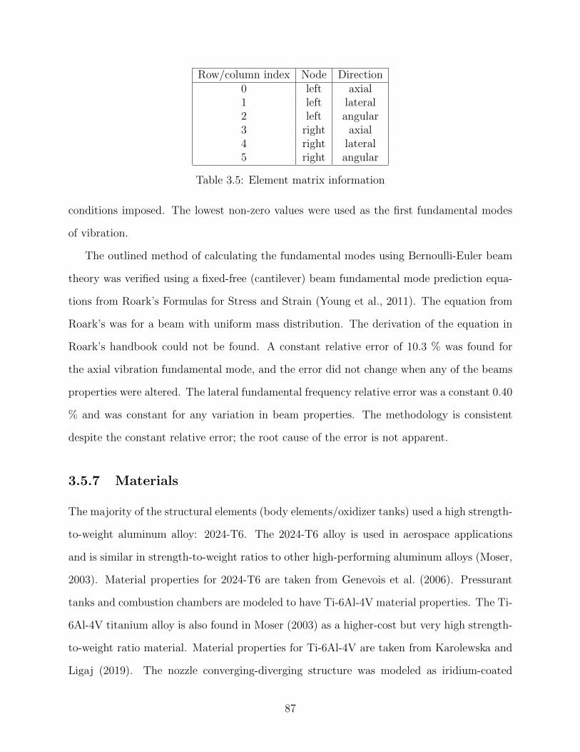
Row/column index Node Direction0 left axial1 left lateral2 left angular3 right axial4 right lateral5 right angular

Table 3.5: Element matrix information

conditions imposed. The lowest non-zero values were used as the first fundamental modes

of vibration.

The outlined method of calculating the fundamental modes using Bernoulli-Euler beam

theory was verified using a fixed-free (cantilever) beam fundamental mode prediction equa-

tions from Roark’s Formulas for Stress and Strain (Young et al., 2011). The equation from

Roark’s was for a beam with uniform mass distribution. The derivation of the equation in

Roark’s handbook could not be found. A constant relative error of 10.3 % was found for

the axial vibration fundamental mode, and the error did not change when any of the beams

properties were altered. The lateral fundamental frequency relative error was a constant 0.40

% and was constant for any variation in beam properties. The methodology is consistent

despite the constant relative error; the root cause of the error is not apparent.

3.5.7 Materials

The majority of the structural elements (body elements/oxidizer tanks) used a high strength-

to-weight aluminum alloy: 2024-T6. The 2024-T6 alloy is used in aerospace applications

and is similar in strength-to-weight ratios to other high-performing aluminum alloys (Moser,

2003). Material properties for 2024-T6 are taken from Genevois et al. (2006). Pressurant

tanks and combustion chambers are modeled to have Ti-6Al-4V material properties. The Ti-

6Al-4V titanium alloy is also found in Moser (2003) as a higher-cost but very high strength-

to-weight ratio material. Material properties for Ti-6Al-4V are taken from Karolewska and

Ligaj (2019). The nozzle converging-diverging structure was modeled as iridium-coated

87

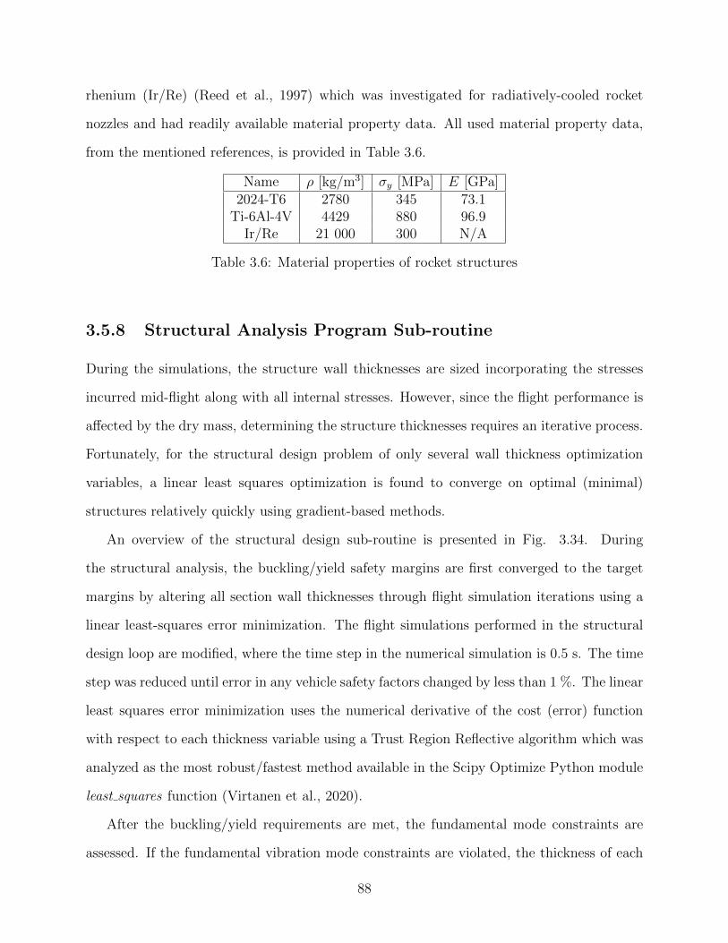
rhenium (Ir/Re) (Reed et al., 1997) which was investigated for radiatively-cooled rocket

nozzles and had readily available material property data. All used material property data,

from the mentioned references, is provided in Table 3.6.

Name ρ [kg/m3] σy [MPa] E [GPa]2024-T6 2780 345 73.1

Ti-6Al-4V 4429 880 96.9Ir/Re 21 000 300 N/A

Table 3.6: Material properties of rocket structures

3.5.8 Structural Analysis Program Sub-routine

During the simulations, the structure wall thicknesses are sized incorporating the stresses

incurred mid-flight along with all internal stresses. However, since the flight performance is

affected by the dry mass, determining the structure thicknesses requires an iterative process.

Fortunately, for the structural design problem of only several wall thickness optimization

variables, a linear least squares optimization is found to converge on optimal (minimal)

structures relatively quickly using gradient-based methods.

An overview of the structural design sub-routine is presented in Fig. 3.34. During

the structural analysis, the buckling/yield safety margins are first converged to the target

margins by altering all section wall thicknesses through flight simulation iterations using a

linear least-squares error minimization. The flight simulations performed in the structural

design loop are modified, where the time step in the numerical simulation is 0.5 s. The time

step was reduced until error in any vehicle safety factors changed by less than 1 %. The linear

least squares error minimization uses the numerical derivative of the cost (error) function

with respect to each thickness variable using a Trust Region Reflective algorithm which was

analyzed as the most robust/fastest method available in the Scipy Optimize Python module

least squares function (Virtanen et al., 2020).

After the buckling/yield requirements are met, the fundamental mode constraints are

assessed. If the fundamental vibration mode constraints are violated, the thickness of each

88

section are modified in another local-level optimization. The thickness lower bounds for the

modal analysis are taken from the output of the strength-based structural analysis. The

local level optimization minimizes structure mass while adjusting all section thicknesses to

meet the desired rigidity criteria. The cost function for the local level optimization has scalar

value, but since the problem is multi-objective the cost function weights are adjusted until

adequate vibrational mode convergence is met (< 1%). The cost function for the modal

analysis, after trial and error, is the dry mass plus 10 times the error for each respective

vibrational mode from the target, if the respective constraint is violated (Eqn. 3.93). The

algorithm of choice is the L-BFGS-B algorithm in the Scipy Optimize module minimize

function (Virtanen et al., 2020). The L-BFGS-B algorithm was chosen as the problem was

non-linear and the solutions may not exist at the extremes and have local optima. The

limited memory, bounded BFGS algorithm is in the class of quasi-Newton’s method and was

found to quickly converge on thickness values for a modal analysis compared to other non-

linear methods available in the Scipy Optimize module. The good performance is attributed

to the smoothness of the objective function and the algorithm’s ability to handle many

variables. The modal analysis and sizing is relatively fast as no flight simulations are needed

and all required sub-processes are analytic.

Costmodal = mdry + 10[faxial,calc. − faxial,desired] + 10[fbending,calc. − fbending,desired] (3.93)

Typically, thin sections, such as the engine skirt or upper stage portions that have low

strength requirements are the thinnest and offer the greatest rigidity increase for additional

inert mass, so are found to be the altered members. Once the modal constraints are met,

while inert mass is minimized, the thickness generated are assumed a lower bound for a

strength-based structural analysis. The strength-based analysis is re-done ensuring margins

are at or above the desired safety factors. The two structural sub-routines are, in general,

89

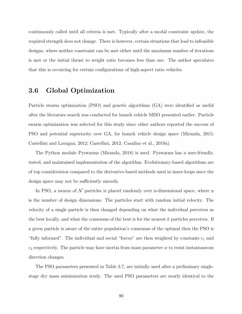
continuously called until all criteria is met. Typically after a modal constraint update, the

required strength does not change. There is however, certain situations that lead to infeasible

designs, where neither constraint can be met either until the maximum number of iterations

is met or the initial thrust to weight ratio becomes less than one. The author speculates

that this is occurring for certain configurations of high-aspect ratio vehicles.

3.6 Global Optimization

Particle swarm optimization (PSO) and genetic algorithms (GA) were identified as useful

after the literature search was conducted for launch vehicle MDO presented earlier. Particle

swarm optimization was selected for this study since other authors reported the success of

PSO and potential superiority over GA, for launch vehicle design space (Miranda, 2015;

Castellini and Lavagna, 2012; Castellini, 2012; Casalino et al., 2019a).

The Python module Pyswarms (Miranda, 2018) is used. Pyswarms has a user-friendly,

tested, and maintained implementation of the algorithm. Evolutionary-based algorithms are

of top consideration compared to the derivative-based methods used in inner-loops since the

design space may not be sufficiently smooth.

In PSO, a swarm of N particles is placed randomly over n-dimensional space, where n

is the number of design dimensions. The particles start with random initial velocity. The

velocity of a single particle is then changed depending on what the individual perceives as

the best locally, and what the consensus of the best is for the nearest k particles perceives. If

a given particle is aware of the entire population’s consensus of the optimal then the PSO is

“fully informed”. The individual and social “forces” are then weighted by constants c1 and

c2 respectively. The particle may have inertia from mass parameter w to resist instantaneous

direction changes.

The PSO parameters presented in Table 3.7, are initially used after a preliminary single-

stage dry mass minimization study. The used PSO parameters are nearly identical to the

90

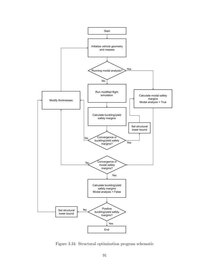
Initialize vehicle geometry and masses

Run modified flight simulation

Convergence in buckling/yield safety

margins?

Convergence in modal safety

margins?

YesNo

Running modal analysis?

No

Yes

Positive buckling/yield safety

margins?

No

No

Yes

Yes

Calculate buckling/yield safety margins

Calculate modal safety margins

Modal analysis = TrueModify thicknesses

Calculate buckling/yield safety margins

Modal analysis = False

End

Start

Set structural lower bound

Set structural lower bound

Figure 3.34: Structural optimization program schematic

91

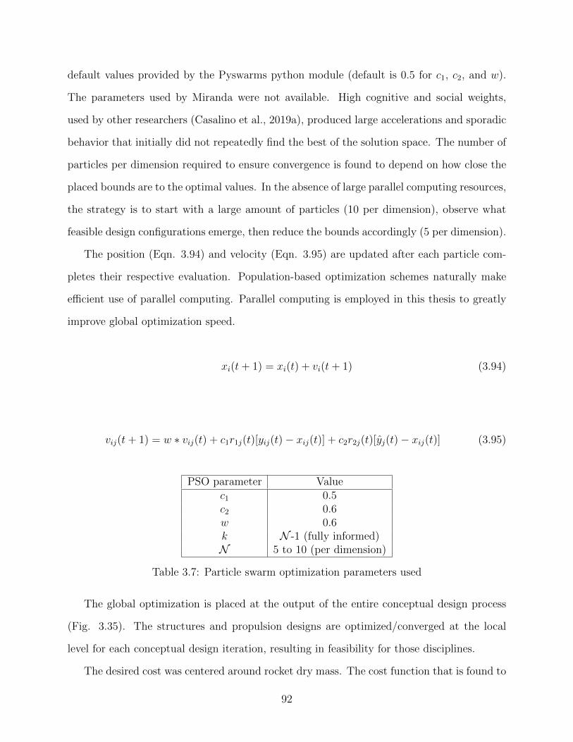
default values provided by the Pyswarms python module (default is 0.5 for c1, c2, and w).

The parameters used by Miranda were not available. High cognitive and social weights,

used by other researchers (Casalino et al., 2019a), produced large accelerations and sporadic

behavior that initially did not repeatedly find the best of the solution space. The number of

particles per dimension required to ensure convergence is found to depend on how close the

placed bounds are to the optimal values. In the absence of large parallel computing resources,

the strategy is to start with a large amount of particles (10 per dimension), observe what

feasible design configurations emerge, then reduce the bounds accordingly (5 per dimension).

The position (Eqn. 3.94) and velocity (Eqn. 3.95) are updated after each particle com-

pletes their respective evaluation. Population-based optimization schemes naturally make

efficient use of parallel computing. Parallel computing is employed in this thesis to greatly

improve global optimization speed.

xi(t+ 1) = xi(t) + vi(t+ 1) (3.94)

vij(t+ 1) = w ∗ vij(t) + c1r1j(t)[yij(t)− xij(t)] + c2r2j(t)[yj(t)− xij(t)] (3.95)

PSO parameter Valuec1 0.5c2 0.6w 0.6k N -1 (fully informed)N 5 to 10 (per dimension)

Table 3.7: Particle swarm optimization parameters used

The global optimization is placed at the output of the entire conceptual design process

(Fig. 3.35). The structures and propulsion designs are optimized/converged at the local

level for each conceptual design iteration, resulting in feasibility for those disciplines.

The desired cost was centered around rocket dry mass. The cost function that is found to

92

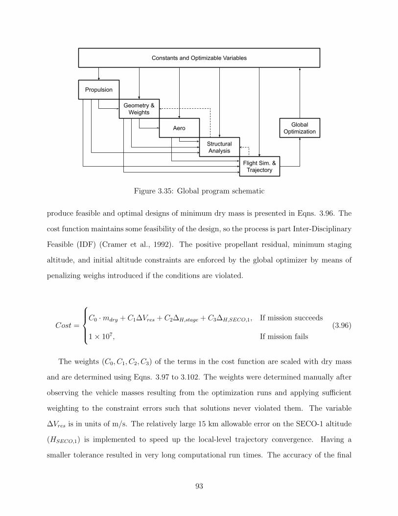
Propulsion

Geometry &Weights

Aero

Structural Analysis

Flight Sim. &Trajectory

Global Optimization

Constants and Optimizable Variables

Figure 3.35: Global program schematic

produce feasible and optimal designs of minimum dry mass is presented in Eqns. 3.96. The

cost function maintains some feasibility of the design, so the process is part Inter-Disciplinary

Feasible (IDF) (Cramer et al., 1992). The positive propellant residual, minimum staging

altitude, and initial altitude constraints are enforced by the global optimizer by means of

penalizing weighs introduced if the conditions are violated.

Cost =

C0 ·mdry + C1∆Vres + C2∆H,stage + C3∆H,SECO,1, If mission succeeds

1× 107, If mission fails

(3.96)

The weights (C0, C1, C2, C3) of the terms in the cost function are scaled with dry mass

and are determined using Eqns. 3.97 to 3.102. The weights were determined manually after

observing the vehicle masses resulting from the optimization runs and applying sufficient

weighting to the constraint errors such that solutions never violated them. The variable

∆Vres is in units of m/s. The relatively large 15 km allowable error on the SECO-1 altitude

(HSECO,1) is implemented to speed up the local-level trajectory convergence. Having a

smaller tolerance resulted in very long computational run times. The accuracy of the final

93

orbit is unaffected by the inaccurate initial altitude. The initial burn to reach the orbit

apogee and the circularization burn can accurately provide the required orbit since they are

accomplished by truncating burn times. The staging altitude constraint (Eqn. 3.100) is first

implemented such that the upper stage flight is outside of the allowed maximum dynamic

pressure ranges, and the load formulation and trajectory formulation assumptions are kept

valid. A 30 km staging altitude (Hstaging) constraint was implemented as it was observed

to typically be after the maximum dynamic pressure point of the vehicle’s flight. Staging

altitudes are later observed, for optimal configurations, to be beyond 50 km above ground

level. The encountered staging altitudes are driven by dry mass minimization rather than

enforced constraints, so the constraint is ultimately unused. At 50 km altitude, the dynamic

pressure is far below the maximum, for the encountered speeds at staging of 2-3 km/s.

C0 = 100 (3.97)

C1 =

100 ·mdry, ∆Vres < 0

−0.1, ∆Vres ≥ 0

(3.98)

C2 =

mdry100

, ∆H,stage < 0

0, ∆H,stage ≥ 0

(3.99)

∆H,staging = Hstaging −Hstaging,minimum [m] (3.100)

C3 =

mdry100

(|∆H,SECO,1|

15000− 1), |∆H,SECO,1| ≥ 15000

0, |∆H,SECO,1| < 15000

(3.101)

∆H,SECO,1 = HSECO,1 −HSECO,1,target [m] (3.102)

94

Chapter 4

Results

4.1 Single-stage Parametric Studies

Parametric studies of single-stage, sub-orbital rocket vehicle configurations are described in

this chapter. The goals of the studies are to identify design trends, observe if the optima exist

at the extremes, and identify physical bounds for use within the computationally-intensive

multi-stage global optimization studies. Back-fill-pressure-fed and electric pump-fed systems

are investigated for LOx/paraffin and N2O/paraffin HREs to be used in these assessments.

Additionally, a self-pressurizing feed system is investigated for N2O/paraffin HRE configu-

rations. Helium is used for the pressurant gas when required as it resits dissolving in the

oxidizers, compared to other inert gases (Zucker et al., 1989). Helium also has a low specific

heat ratio and molecular weight relative to other common pressurant gases resulting in less

inert mass and higher performance. The parametric studies are conducted holding all other

design variables constant, except the burn time. All parametric studies are conducted with

a range of burn times and the final results are presented with the optimal burn time for each

parameter value. Simulating over a range of burn times is done to remove its influence on

the results, as it was found to interact with different design variables, especially if the vehicle

scale changed drastically through parameter sweeps.

95

The default outer diameter, in this parametric study, is set to the minimum possible given

vehicle geometry constraints (nozzles and combustion chambers). The minimum diameter

is used after initial results showed it is likely the most optimal and will lead to better

comparison across different scales (dry mass values). For all other design variables, when

they are not being varied, are taken as the value in Table 4.1. The OFav and Pup values in

Table 4.1 are used as they are conjectured to be optimal or near optimal. For a reasonable

physical upper bound, the pressurant initial pressure is 18 MPa, as this is a common gas

storage pressure found in gas cylinders and is a typical service pressure for standard fittings

and piping (Hermsen and Zandbergen, 2017). The pressurant initial temperature is chosen

to correspond to standard conditions (15◦ C). The nozzle exit pressure of 50 kPa is used as it

is desired to be minimized, while still meeting the Summerfield criteria (Stark, 2005). The 10

kPa margin is used to ensure variations in mass flow, caused by OF shift, did not reduce the

chamber pressure and subsequently nozzle exit pressure below the 40 % of standard sea level

ambient pressure. Perhaps for a smaller total impulse scale vehicle, the optimal expansion

may be a higher exit pressure, but this is not the case for the very high-flying rockets being

considered here. The initial oxidizer temperature, when the feed system is either back-fill

or pump-fed, is presumed to be the oxidizer normal boiling point. The normal boiling point

temperature is selected for practical purposes as the temperature can be easily controlled, if

heating occurs, by allowing the oxidizer to boil off as required to remove energy supplied by

the ambient environment. The self-pressurizing N2O initial temperature value is arbitrarily

chosen. All other constants are taken from Tables B.1, B.2, and B.3 listed in the appendix.

The parametric studies being done here use the vehicle’s ∆V from final altitude and

velocity to quantify performance. The ∆V in these parametric studies (Delivered ∆V ) is

calculated from an energy balance using the vehicle final altitude (∆H), which occurs at

zero velocity due to the vertical, non-perturbed flight. The delivered ∆V is calculate from

the following: ∆V =√

2µE( 1rE− 1

rE+∆H), and rE is the Earth radius. The rocket speed,

immediately post-burn, is not used as the change in velocity (∆V ), in order to account

96

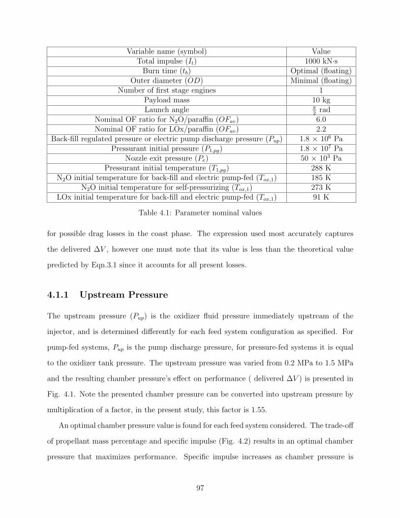
Variable name (symbol) ValueTotal impulse (It) 1000 kN·s

Burn time (tb) Optimal (floating)Outer diameter (OD) Minimal (floating)

Number of first stage engines 1Payload mass 10 kgLaunch angle π

2rad

Nominal OF ratio for N2O/paraffin (OFav) 6.0Nominal OF ratio for LOx/paraffin (OFav) 2.2

Back-fill regulated pressure or electric pump discharge pressure (Pup) 1.8 × 106 PaPressurant initial pressure (P1,pg) 1.8 × 107 Pa

Nozzle exit pressure (Pe) 50 × 103 PaPressurant initial temperature (T1,pg) 288 K

N2O initial temperature for back-fill and electric pump-fed (Tox,1) 185 KN2O initial temperature for self-pressurizing (Tox,1) 273 K

LOx initial temperature for back-fill and electric pump-fed (Tox,1) 91 K

Table 4.1: Parameter nominal values

for possible drag losses in the coast phase. The expression used most accurately captures

the delivered ∆V , however one must note that its value is less than the theoretical value

predicted by Eqn.3.1 since it accounts for all present losses.

4.1.1 Upstream Pressure

The upstream pressure (Pup) is the oxidizer fluid pressure immediately upstream of the

injector, and is determined differently for each feed system configuration as specified. For

pump-fed systems, Pup is the pump discharge pressure, for pressure-fed systems it is equal

to the oxidizer tank pressure. The upstream pressure was varied from 0.2 MPa to 1.5 MPa

and the resulting chamber pressure’s effect on performance ( delivered ∆V ) is presented in

Fig. 4.1. Note the presented chamber pressure can be converted into upstream pressure by

multiplication of a factor, in the present study, this factor is 1.55.

An optimal chamber pressure value is found for each feed system considered. The trade-off

of propellant mass percentage and specific impulse (Fig. 4.2) results in an optimal chamber

pressure that maximizes performance. Specific impulse increases as chamber pressure is

97

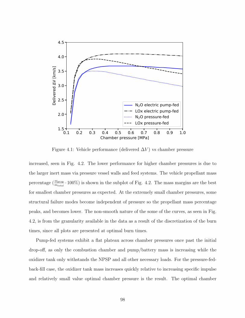
0.1 0.2 0.3 0.4 0.5 0.6 0.7 0.8 0.9 1.0Chamber pressure [MPa]

1.5

2.0

2.5

3.0

3.5

4.0

4.5

Deliv

ered

V

[km

/s]

N2O electric pump-fedLOx electric pump-fedN2O pressure-fedLOx pressure-fed

Figure 4.1: Vehicle performance (delivered ∆V ) vs chamber pressure

increased, seen in Fig. 4.2. The lower performance for higher chamber pressures is due to

the larger inert mass via pressure vessel walls and feed systems. The vehicle propellant mass

percentage (mpropmtotal

·100%) is shown in the subplot of Fig. 4.2. The mass margins are the best

for smallest chamber pressures as expected. At the extremely small chamber pressures, some

structural failure modes become independent of pressure so the propellant mass percentage

peaks, and becomes lower. The non-smooth nature of the some of the curves, as seen in Fig.

4.2, is from the granularity available in the data as a result of the discretization of the burn

times, since all plots are presented at optimal burn times.

Pump-fed systems exhibit a flat plateau across chamber pressures once past the initial

drop-off, as only the combustion chamber and pump/battery mass is increasing while the

oxidizer tank only withstands the NPSP and all other necessary loads. For the pressure-fed-

back-fill case, the oxidizer tank mass increases quickly relative to increasing specific impulse

and relatively small value optimal chamber pressure is the result. The optimal chamber

98

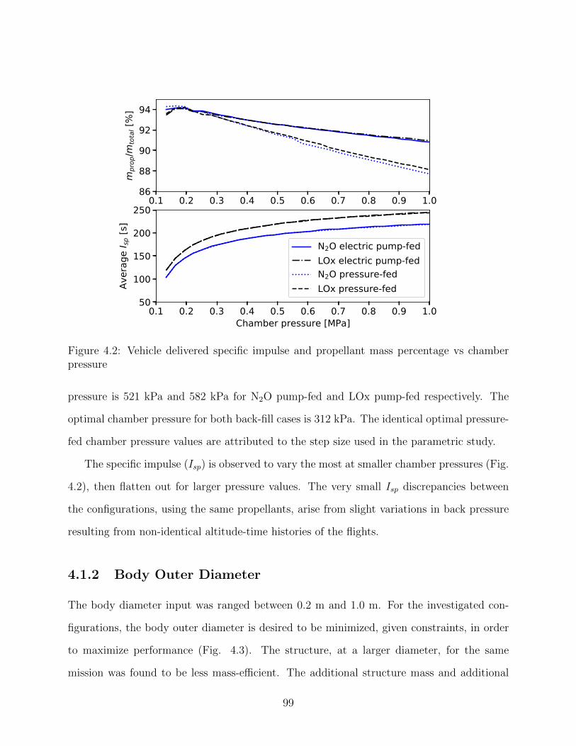
0.1 0.2 0.3 0.4 0.5 0.6 0.7 0.8 0.9 1.086

88

90

92

94m

prop

/mto

tal [

%]

0.1 0.2 0.3 0.4 0.5 0.6 0.7 0.8 0.9 1.0Chamber pressure [MPa]

50

100

150

200

250

Aver

age

I sp [s

]

N2O electric pump-fedLOx electric pump-fedN2O pressure-fedLOx pressure-fed

Figure 4.2: Vehicle delivered specific impulse and propellant mass percentage vs chamberpressure

pressure is 521 kPa and 582 kPa for N2O pump-fed and LOx pump-fed respectively. The

optimal chamber pressure for both back-fill cases is 312 kPa. The identical optimal pressure-

fed chamber pressure values are attributed to the step size used in the parametric study.

The specific impulse (Isp) is observed to vary the most at smaller chamber pressures (Fig.

4.2), then flatten out for larger pressure values. The very small Isp discrepancies between

the configurations, using the same propellants, arise from slight variations in back pressure

resulting from non-identical altitude-time histories of the flights.

4.1.2 Body Outer Diameter

The body diameter input was ranged between 0.2 m and 1.0 m. For the investigated con-

figurations, the body outer diameter is desired to be minimized, given constraints, in order

to maximize performance (Fig. 4.3). The structure, at a larger diameter, for the same

mission was found to be less mass-efficient. The additional structure mass and additional

99

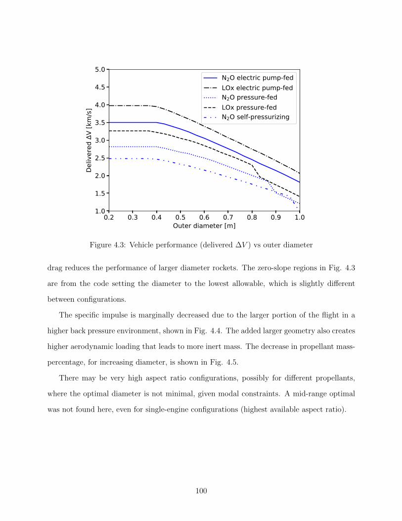
0.2 0.3 0.4 0.5 0.6 0.7 0.8 0.9 1.0Outer diameter [m]

1.0

1.5

2.0

2.5

3.0

3.5

4.0

4.5

5.0

Deliv

ered

V

[km

/s]

N2O electric pump-fedLOx electric pump-fedN2O pressure-fedLOx pressure-fedN2O self-pressurizing

Figure 4.3: Vehicle performance (delivered ∆V ) vs outer diameter

drag reduces the performance of larger diameter rockets. The zero-slope regions in Fig. 4.3

are from the code setting the diameter to the lowest allowable, which is slightly different

between configurations.

The specific impulse is marginally decreased due to the larger portion of the flight in a

higher back pressure environment, shown in Fig. 4.4. The added larger geometry also creates

higher aerodynamic loading that leads to more inert mass. The decrease in propellant mass-

percentage, for increasing diameter, is shown in Fig. 4.5.

There may be very high aspect ratio configurations, possibly for different propellants,

where the optimal diameter is not minimal, given modal constraints. A mid-range optimal

was not found here, even for single-engine configurations (highest available aspect ratio).

100

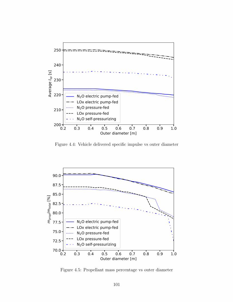
0.2 0.3 0.4 0.5 0.6 0.7 0.8 0.9 1.0Outer diameter [m]

200

210

220

230

240

250Av

erag

e I sp

[s]

N2O electric pump-fedLOx electric pump-fedN2O pressure-fedLOx pressure-fedN2O self-pressurizing

Figure 4.4: Vehicle delivered specific impulse vs outer diameter

0.2 0.3 0.4 0.5 0.6 0.7 0.8 0.9 1.0Outer diameter [m]

70.0

72.5

75.0

77.5

80.0

82.5

85.0

87.5

90.0

mpr

op/m

tota

l [%

]

N2O electric pump-fedLOx electric pump-fedN2O pressure-fedLOx pressure-fedN2O self-pressurizing

Figure 4.5: Propellant mass percentage vs outer diameter

101

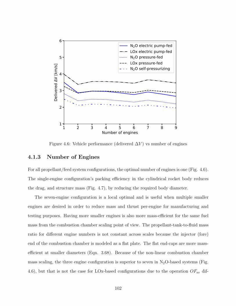
1 2 3 4 5 6 7 8 9Number of engines

1

2

3

4

5

6

Deliv

ered

V

[km

/s]

N2O electric pump-fedLOx electric pump-fedN2O pressure-fedLOx pressure-fedN2O self-pressurizing

Figure 4.6: Vehicle performance (delivered ∆V ) vs number of engines

4.1.3 Number of Engines

For all propellant/feed system configurations, the optimal number of engines is one (Fig. 4.6).

The single-engine configuration’s packing efficiency in the cylindrical rocket body reduces

the drag, and structure mass (Fig. 4.7), by reducing the required body diameter.

The seven-engine configuration is a local optimal and is useful when multiple smaller

engines are desired in order to reduce mass and thrust per-engine for manufacturing and

testing purposes. Having more smaller engines is also more mass-efficient for the same fuel

mass from the combustion chamber scaling point of view. The propellant-tank-to-fluid mass

ratio for different engine numbers is not constant across scales because the injector (fore)

end of the combustion chamber is modeled as a flat plate. The flat end-caps are more mass-

efficient at smaller diameters (Eqn. 3.68). Because of the non-linear combustion chamber

mass scaling, the three engine configuration is superior to seven in N2O-based systems (Fig.

4.6), but that is not the case for LOx-based configurations due to the operation OFav dif-

102

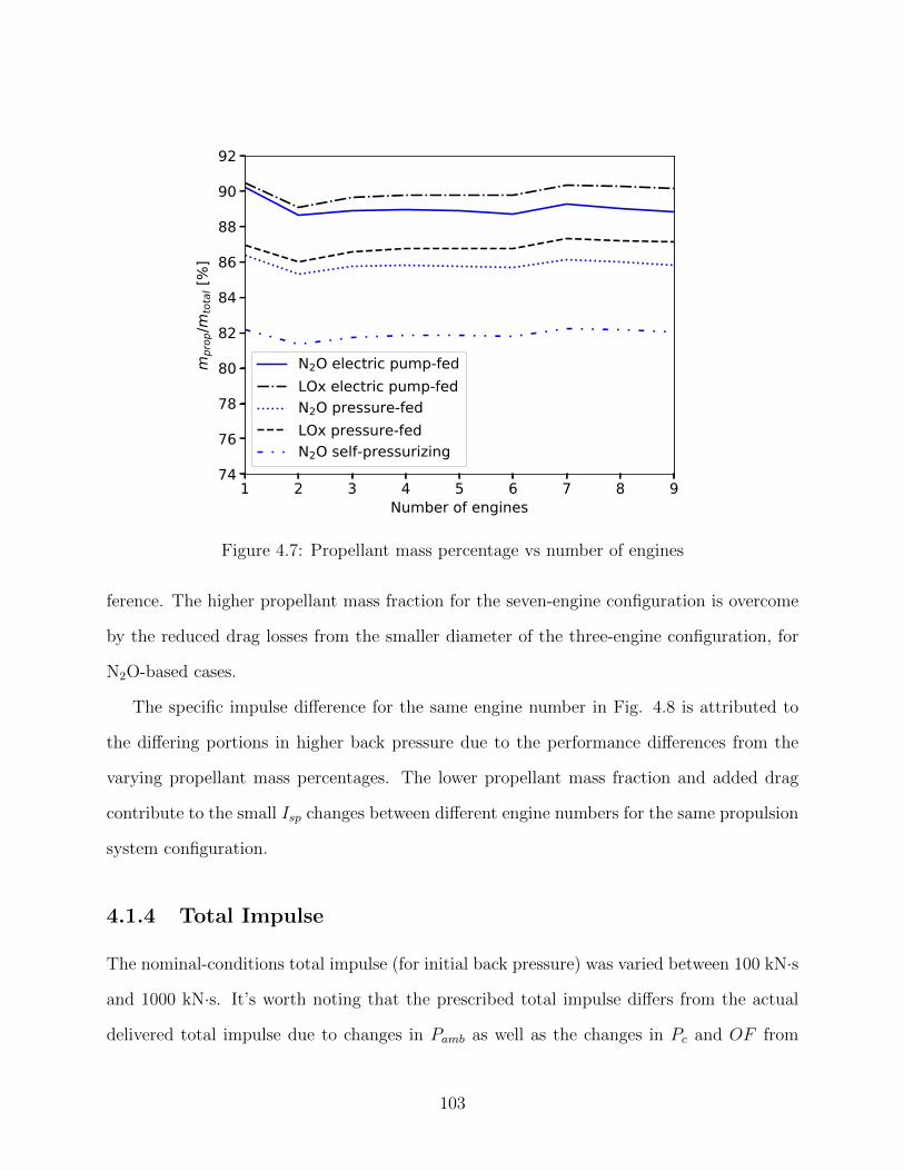
1 2 3 4 5 6 7 8 9Number of engines

74

76

78

80

82

84

86

88

90

92

mpr

op/m

tota

l [%

]

N2O electric pump-fedLOx electric pump-fedN2O pressure-fedLOx pressure-fedN2O self-pressurizing

Figure 4.7: Propellant mass percentage vs number of engines

ference. The higher propellant mass fraction for the seven-engine configuration is overcome

by the reduced drag losses from the smaller diameter of the three-engine configuration, for

N2O-based cases.

The specific impulse difference for the same engine number in Fig. 4.8 is attributed to

the differing portions in higher back pressure due to the performance differences from the

varying propellant mass percentages. The lower propellant mass fraction and added drag

contribute to the small Isp changes between different engine numbers for the same propulsion

system configuration.

4.1.4 Total Impulse

The nominal-conditions total impulse (for initial back pressure) was varied between 100 kN·s

and 1000 kN·s. It’s worth noting that the prescribed total impulse differs from the actual

delivered total impulse due to changes in Pamb as well as the changes in Pc and OF from

103

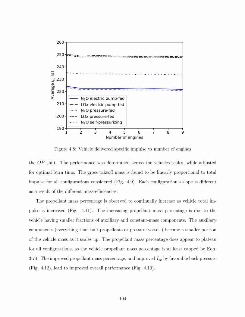
1 2 3 4 5 6 7 8 9Number of engines

190

200

210

220

230

240

250

260

Aver

age

I sp [s

]

N2O electric pump-fedLOx electric pump-fedN2O pressure-fedLOx pressure-fedN2O self-pressurizing

Figure 4.8: Vehicle delivered specific impulse vs number of engines

the OF shift. The performance was determined across the vehicles scales, while adjusted

for optimal burn time. The gross takeoff mass is found to be linearly proportional to total

impulse for all configurations considered (Fig. 4.9). Each configuration’s slope is different

as a result of the different mass-efficiencies.

The propellant mass percentage is observed to continually increase as vehicle total im-

pulse is increased (Fig. 4.11). The increasing propellant mass percentage is due to the

vehicle having smaller fractions of auxiliary and constant-mass components. The auxiliary

components (everything that isn’t propellants or pressure vessels) become a smaller portion

of the vehicle mass as it scales up. The propellant mass percentage does appear to plateau

for all configurations, as the vehicle propellant mass percentage is at least capped by Eqn.

3.74. The improved propellant mass percentage, and improved Isp by favorable back pressure

(Fig. 4.12), lead to improved overall performance (Fig. 4.10).

104

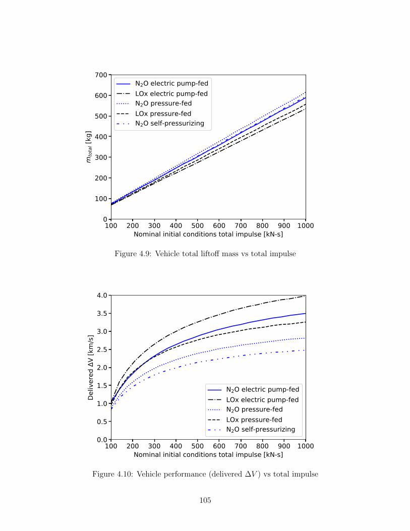
100 200 300 400 500 600 700 800 900 1000Nominal initial conditions total impulse [kN-s]

0

100

200

300

400

500

600

700m

tota

l [kg

]N2O electric pump-fedLOx electric pump-fedN2O pressure-fedLOx pressure-fedN2O self-pressurizing

Figure 4.9: Vehicle total liftoff mass vs total impulse

100 200 300 400 500 600 700 800 900 1000Nominal initial conditions total impulse [kN-s]

0.0

0.5

1.0

1.5

2.0

2.5

3.0

3.5

4.0

Deliv

ered

V

[km

/s]

N2O electric pump-fedLOx electric pump-fedN2O pressure-fedLOx pressure-fedN2O self-pressurizing

Figure 4.10: Vehicle performance (delivered ∆V ) vs total impulse

105

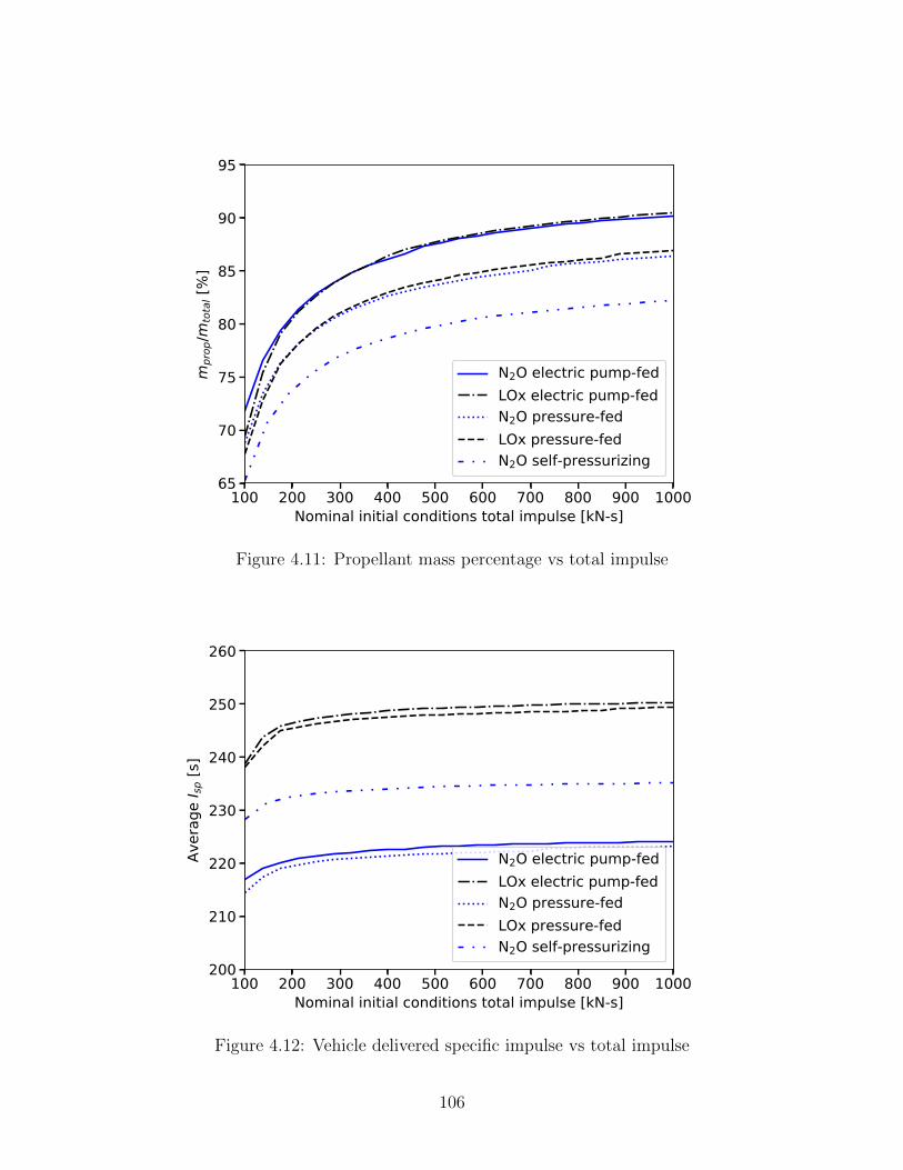
100 200 300 400 500 600 700 800 900 1000Nominal initial conditions total impulse [kN-s]

65

70

75

80

85

90

95

mpr

op/m

tota

l [%

]

N2O electric pump-fedLOx electric pump-fedN2O pressure-fedLOx pressure-fedN2O self-pressurizing

Figure 4.11: Propellant mass percentage vs total impulse

100 200 300 400 500 600 700 800 900 1000Nominal initial conditions total impulse [kN-s]

200

210

220

230

240

250

260

Aver

age

I sp [s

]

N2O electric pump-fedLOx electric pump-fedN2O pressure-fedLOx pressure-fedN2O self-pressurizing

Figure 4.12: Vehicle delivered specific impulse vs total impulse

106

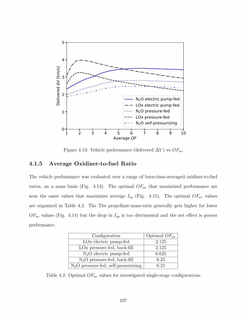
1 2 3 4 5 6 7 8 9 10Average OF

0

1

2

3

4

5

Deliv

ered

V

[km

/s]

N2O electric pump-fedLOx electric pump-fedN2O pressure-fedLOx pressure-fedN2O self-pressurizing

Figure 4.13: Vehicle performance (delivered ∆V ) vs OFav

4.1.5 Average Oxidizer-to-fuel Ratio

The vehicle performance was evaluated over a range of burn-time-averaged oxidizer-to-fuel

ratios, on a mass basis (Fig. 4.13). The optimal OFav that maximized performance are

near the same values that maximizes average Isp (Fig. 4.15). The optimal OFav values

are organized in Table 4.2. The The propellant-mass-ratio generally gets higher for lower

OFav values (Fig. 4.14) but the drop in Isp is too detrimental and the net effect is poorer

performance.

Configuration Optimal OFavLOx electric pump-fed 2.125

LOx pressure-fed, back-fill 2.125N2O electric pump-fed 6.625

N2O pressure-fed, back-fill 6.25N2O pressure-fed, self-pressurizing 6.21

Table 4.2: Optimal OFav values for investigated single-stage configurations

107

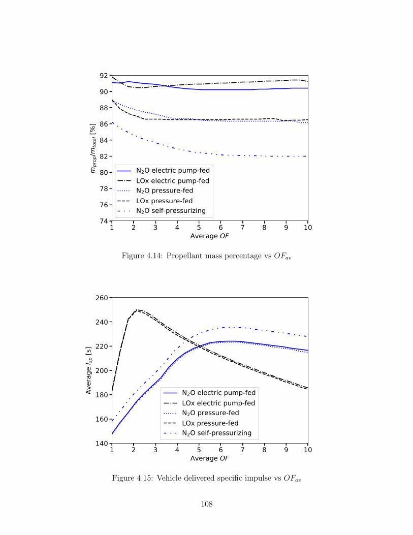
1 2 3 4 5 6 7 8 9 10Average OF

74

76

78

80

82

84

86

88

90

92

mpr

op/m

tota

l [%

]

N2O electric pump-fedLOx electric pump-fedN2O pressure-fedLOx pressure-fedN2O self-pressurizing

Figure 4.14: Propellant mass percentage vs OFav

1 2 3 4 5 6 7 8 9 10Average OF

140

160

180

200

220

240

260

Aver

age

I sp [s

]

N2O electric pump-fedLOx electric pump-fedN2O pressure-fedLOx pressure-fedN2O self-pressurizing

Figure 4.15: Vehicle delivered specific impulse vs OFav

108

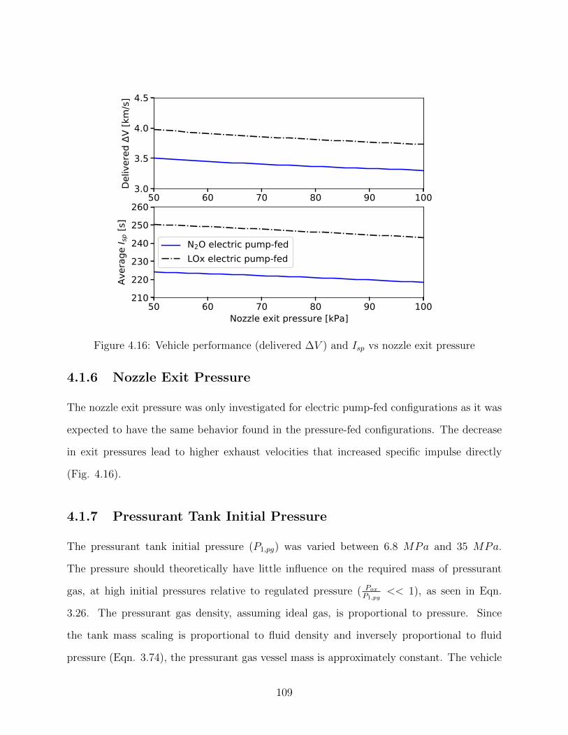
50 60 70 80 90 1003.0

3.5

4.0

4.5

Deliv

ered

V

[km

/s]

50 60 70 80 90 100Nozzle exit pressure [kPa]

210220230240250260

Aver

age

I sp [s

]

N2O electric pump-fedLOx electric pump-fed

Figure 4.16: Vehicle performance (delivered ∆V ) and Isp vs nozzle exit pressure

4.1.6 Nozzle Exit Pressure

The nozzle exit pressure was only investigated for electric pump-fed configurations as it was

expected to have the same behavior found in the pressure-fed configurations. The decrease

in exit pressures lead to higher exhaust velocities that increased specific impulse directly

(Fig. 4.16).

4.1.7 Pressurant Tank Initial Pressure

The pressurant tank initial pressure (P1,pg) was varied between 6.8 MPa and 35 MPa.

The pressure should theoretically have little influence on the required mass of pressurant

gas, at high initial pressures relative to regulated pressure ( PoxP1,pg

<< 1), as seen in Eqn.

3.26. The pressurant gas density, assuming ideal gas, is proportional to pressure. Since

the tank mass scaling is proportional to fluid density and inversely proportional to fluid

pressure (Eqn. 3.74), the pressurant gas vessel mass is approximately constant. The vehicle

109

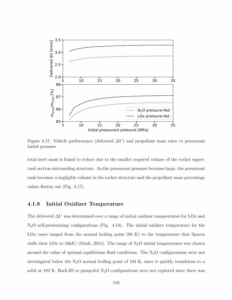
5 10 15 20 25 30 352.0

2.5

3.0

3.5

Deliv

ered

V

[km

/s]

5 10 15 20 25 30 35Initial pressurant pressure [MPa]

85

86

87

88

mpr

op/m

tota

l [%

]

N2O pressure-fedLOx pressure-fed

Figure 4.17: Vehicle performance (delivered ∆V ) and propellant mass ratio vs pressurantinitial pressure

total inert mass is found to reduce due to the smaller required volume of the rocket upper-

tank section surrounding structure. As the pressurant pressure becomes large, the pressurant

tank becomes a negligible volume in the rocket structure and the propellant mass percentage

values flatten out (Fig. 4.17).

4.1.8 Initial Oxidizer Temperature

The delivered ∆V was determined over a range of initial oxidizer temperatures for LOx and

N2O self-pressurizing configurations (Fig. 4.18). The initial oxidizer temperature for the

LOx cases ranged from the normal boiling point (90 K) to the temperature that Spacex

chills their LOx to (66K) (Musk, 2015). The range of N2O initial temperatures was chosen

around the value of optimal equilibrium fluid conditions. The N2O configurations were not

investigated below the N2O normal boiling point of 184 K, since it quickly transitions to a

solid at 182 K. Back-fill or pump-fed N2O configurations were not explored since there was

110

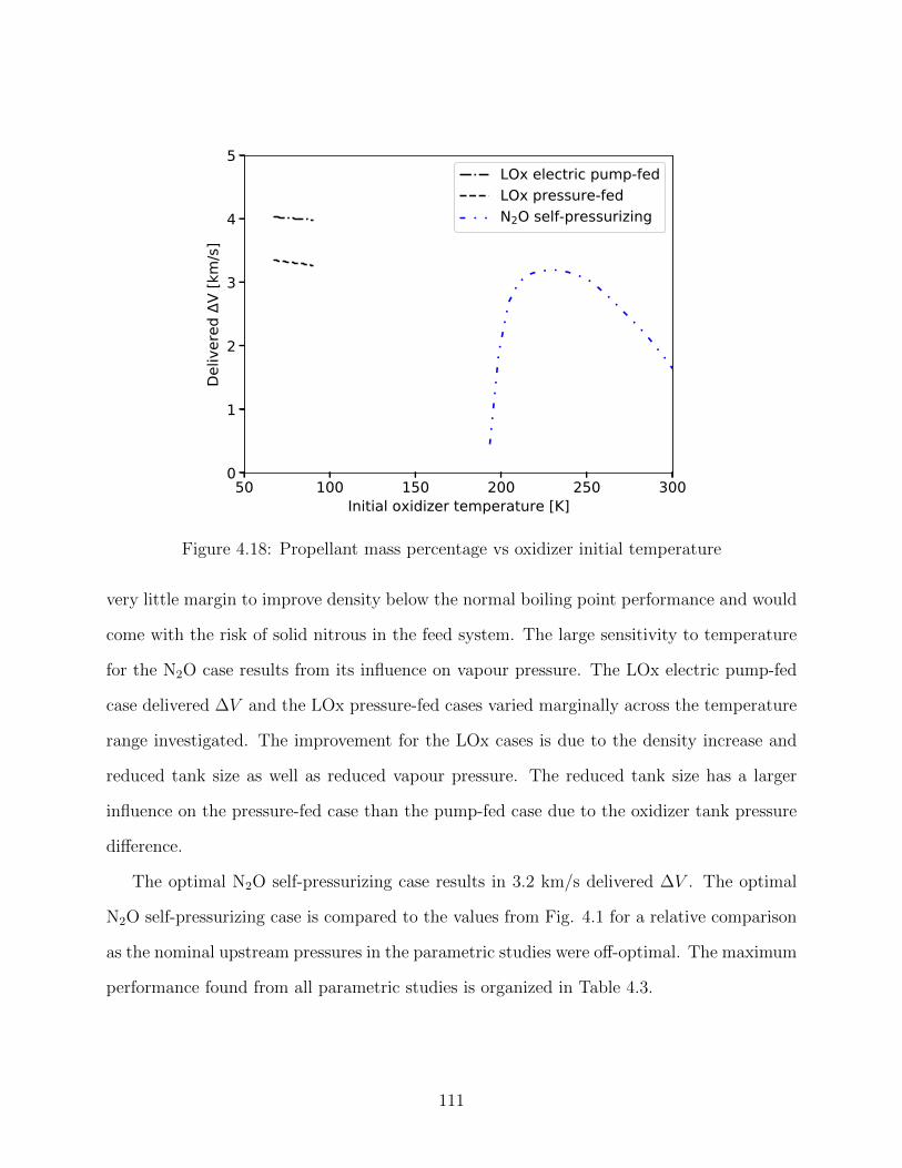
50 100 150 200 250 300Initial oxidizer temperature [K]

0

1

2

3

4

5

Deliv

ered

V

[km

/s]

LOx electric pump-fedLOx pressure-fedN2O self-pressurizing

Figure 4.18: Propellant mass percentage vs oxidizer initial temperature

very little margin to improve density below the normal boiling point performance and would

come with the risk of solid nitrous in the feed system. The large sensitivity to temperature

for the N2O case results from its influence on vapour pressure. The LOx electric pump-fed

case delivered ∆V and the LOx pressure-fed cases varied marginally across the temperature

range investigated. The improvement for the LOx cases is due to the density increase and

reduced tank size as well as reduced vapour pressure. The reduced tank size has a larger

influence on the pressure-fed case than the pump-fed case due to the oxidizer tank pressure

difference.

The optimal N2O self-pressurizing case results in 3.2 km/s delivered ∆V . The optimal

N2O self-pressurizing case is compared to the values from Fig. 4.1 for a relative comparison

as the nominal upstream pressures in the parametric studies were off-optimal. The maximum

performance found from all parametric studies is organized in Table 4.3.

111

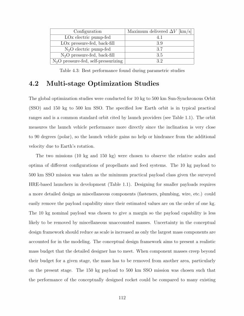
Configuration Maximum delivered ∆V [km/s]LOx electric pump-fed 4.1

LOx pressure-fed, back-fill 3.9N2O electric pump-fed 3.7

N2O pressure-fed, back-fill 3.5N2O pressure-fed, self-pressurizing 3.2

Table 4.3: Best performance found during parametric studies

4.2 Multi-stage Optimization Studies

The global optimization studies were conducted for 10 kg to 500 km Sun-Synchronous Orbit

(SSO) and 150 kg to 500 km SSO. The specified low Earth orbit is in typical practical

ranges and is a common standard orbit cited by launch providers (see Table 1.1). The orbit

measures the launch vehicle performance more directly since the inclination is very close

to 90 degrees (polar), so the launch vehicle gains no help or hindrance from the additional

velocity due to Earth’s rotation.

The two missions (10 kg and 150 kg) were chosen to observe the relative scales and

optima of different configurations of propellants and feed systems. The 10 kg payload to

500 km SSO mission was taken as the minimum practical payload class given the surveyed

HRE-based launchers in development (Table 1.1). Designing for smaller payloads requires

a more detailed design as miscellaneous components (fasteners, plumbing, wire, etc.) could

easily remove the payload capability since their estimated values are on the order of one kg.

The 10 kg nominal payload was chosen to give a margin so the payload capability is less

likely to be removed by miscellaneous unaccounted masses. Uncertainty in the conceptual

design framework should reduce as scale is increased as only the largest mass components are

accounted for in the modeling. The conceptual design framework aims to present a realistic

mass budget that the detailed designer has to meet. When component masses creep beyond

their budget for a given stage, the mass has to be removed from another area, particularly

on the present stage. The 150 kg payload to 500 km SSO mission was chosen such that

the performance of the conceptually designed rocket could be compared to many existing

112

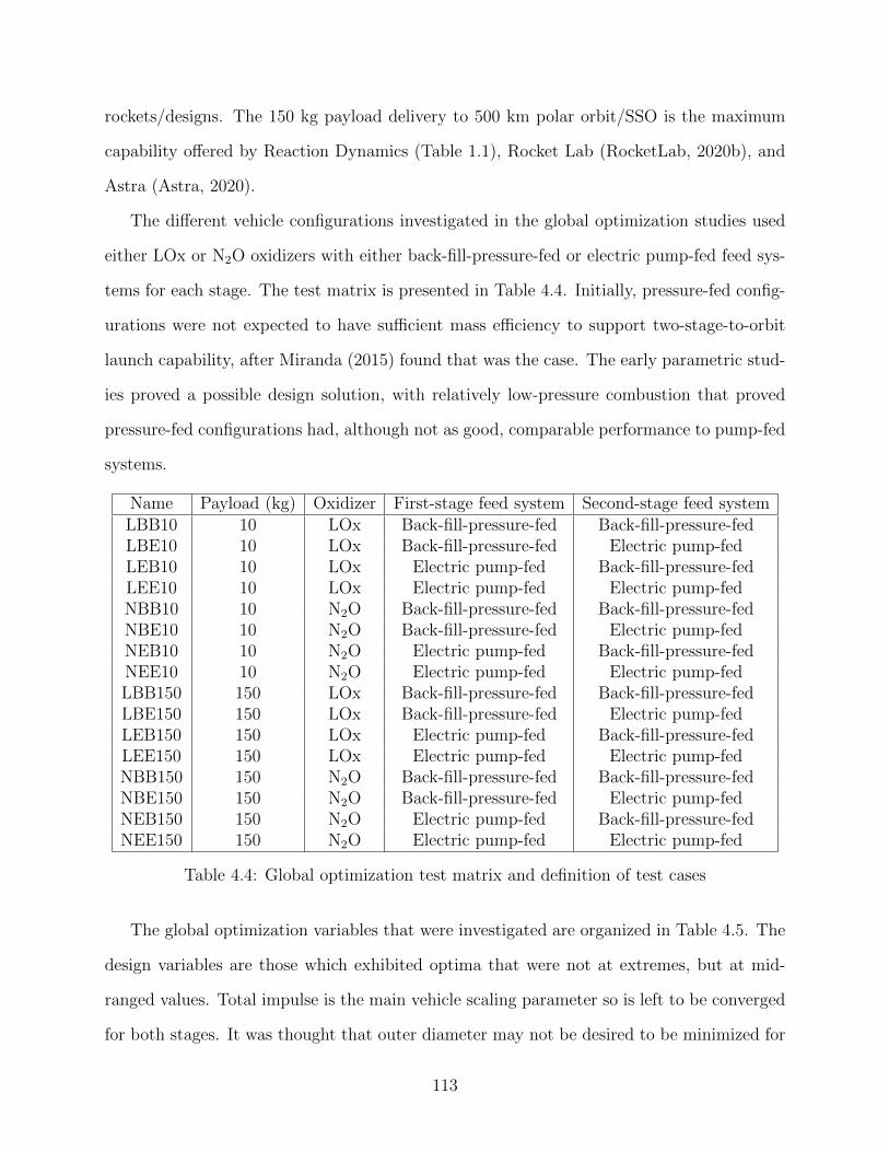
rockets/designs. The 150 kg payload delivery to 500 km polar orbit/SSO is the maximum

capability offered by Reaction Dynamics (Table 1.1), Rocket Lab (RocketLab, 2020b), and

Astra (Astra, 2020).

The different vehicle configurations investigated in the global optimization studies used

either LOx or N2O oxidizers with either back-fill-pressure-fed or electric pump-fed feed sys-

tems for each stage. The test matrix is presented in Table 4.4. Initially, pressure-fed config-

urations were not expected to have sufficient mass efficiency to support two-stage-to-orbit

launch capability, after Miranda (2015) found that was the case. The early parametric stud-

ies proved a possible design solution, with relatively low-pressure combustion that proved

pressure-fed configurations had, although not as good, comparable performance to pump-fed

systems.

Name Payload (kg) Oxidizer First-stage feed system Second-stage feed systemLBB10 10 LOx Back-fill-pressure-fed Back-fill-pressure-fedLBE10 10 LOx Back-fill-pressure-fed Electric pump-fedLEB10 10 LOx Electric pump-fed Back-fill-pressure-fedLEE10 10 LOx Electric pump-fed Electric pump-fedNBB10 10 N2O Back-fill-pressure-fed Back-fill-pressure-fedNBE10 10 N2O Back-fill-pressure-fed Electric pump-fedNEB10 10 N2O Electric pump-fed Back-fill-pressure-fedNEE10 10 N2O Electric pump-fed Electric pump-fedLBB150 150 LOx Back-fill-pressure-fed Back-fill-pressure-fedLBE150 150 LOx Back-fill-pressure-fed Electric pump-fedLEB150 150 LOx Electric pump-fed Back-fill-pressure-fedLEE150 150 LOx Electric pump-fed Electric pump-fedNBB150 150 N2O Back-fill-pressure-fed Back-fill-pressure-fedNBE150 150 N2O Back-fill-pressure-fed Electric pump-fedNEB150 150 N2O Electric pump-fed Back-fill-pressure-fedNEE150 150 N2O Electric pump-fed Electric pump-fed

Table 4.4: Global optimization test matrix and definition of test cases

The global optimization variables that were investigated are organized in Table 4.5. The

design variables are those which exhibited optima that were not at extremes, but at mid-

ranged values. Total impulse is the main vehicle scaling parameter so is left to be converged

for both stages. It was thought that outer diameter may not be desired to be minimized for

113

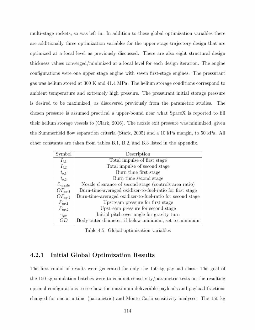
multi-stage rockets, so was left in. In addition to these global optimization variables there

are additionally three optimization variables for the upper stage trajectory design that are

optimized at a local level as previously discussed. There are also eight structural design

thickness values converged/minimized at a local level for each design iteration. The engine

configurations were one upper stage engine with seven first-stage engines. The pressurant

gas was helium stored at 300 K and 41.4 MPa. The helium storage conditions correspond to

ambient temperature and extremely high pressure. The pressurant initial storage pressure

is desired to be maximized, as discovered previously from the parametric studies. The

chosen pressure is assumed practical a upper-bound near what SpaceX is reported to fill

their helium storage vessels to (Clark, 2016). The nozzle exit pressure was minimized, given

the Summerfield flow separation criteria (Stark, 2005) and a 10 kPa margin, to 50 kPa. All

other constants are taken from tables B.1, B.2, and B.3 listed in the appendix.

Symbol DescriptionIt,1 Total impulse of first stageIt,2 Total impulse of second stagetb,1 Burn time first stagetb,2 Burn time second stageδnozzle Nozzle clearance of second stage (controls area ratio)OFav,1 Burn-time-averaged oxidizer-to-fuel-ratio for first stageOFav,2 Burn-time-averaged oxidizer-to-fuel-ratio for second stagePup,1 Upstream pressure for first stagePup,2 Upstream pressure for second stageγpo Initial pitch over angle for gravity turnOD Body outer diameter, if below minimum, set to minimum

Table 4.5: Global optimization variables

4.2.1 Initial Global Optimization Results

The first round of results were generated for only the 150 kg payload class. The goal of

the 150 kg simulation batches were to conduct sensitivity/parametric tests on the resulting

optimal configurations to see how the maximum deliverable payloads and payload fractions

changed for one-at-a-time (parametric) and Monte Carlo sensitivity analyses. The 150 kg

114

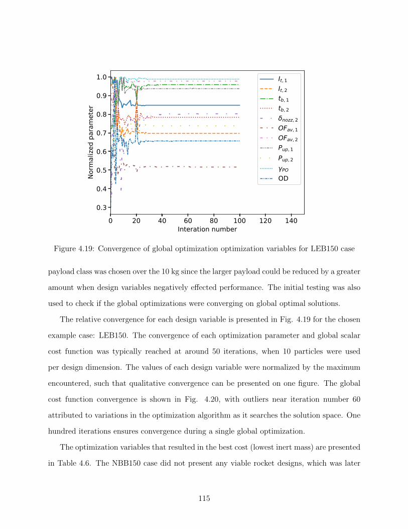
0 20 40 60 80 100 120 140Interation number

0.3

0.4

0.5

0.6

0.7

0.8

0.9

1.0No

rmal

ized

para

met

erIt, 1It, 2tb, 1tb, 2

nozz, 2OFav, 1OFav, 2Pup, 1Pup, 2

PO

OD

Figure 4.19: Convergence of global optimization optimization variables for LEB150 case

payload class was chosen over the 10 kg since the larger payload could be reduced by a greater

amount when design variables negatively effected performance. The initial testing was also

used to check if the global optimizations were converging on global optimal solutions.

The relative convergence for each design variable is presented in Fig. 4.19 for the chosen

example case: LEB150. The convergence of each optimization parameter and global scalar

cost function was typically reached at around 50 iterations, when 10 particles were used

per design dimension. The values of each design variable were normalized by the maximum

encountered, such that qualitative convergence can be presented on one figure. The global

cost function convergence is shown in Fig. 4.20, with outliers near iteration number 60

attributed to variations in the optimization algorithm as it searches the solution space. One

hundred iterations ensures convergence during a single global optimization.

The optimization variables that resulted in the best cost (lowest inert mass) are presented

in Table 4.6. The NBB150 case did not present any viable rocket designs, which was later

115

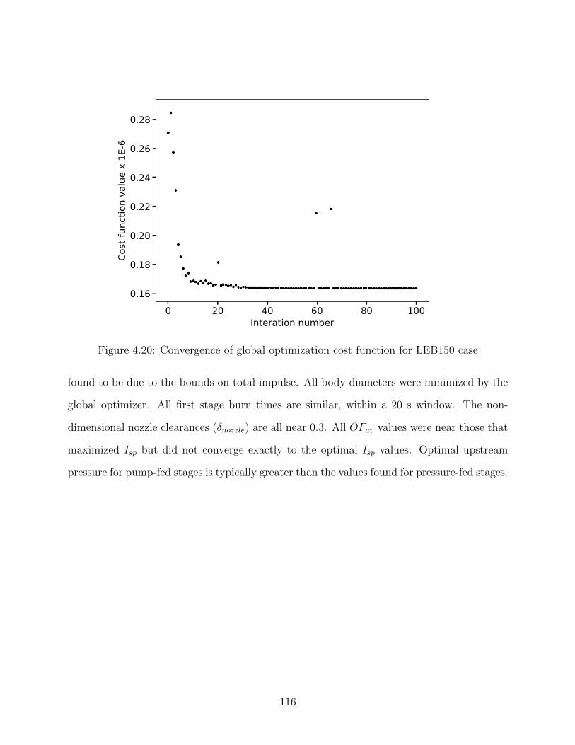
0 20 40 60 80 100Interation number

0.16

0.18

0.20

0.22

0.24

0.26

0.28Co

st fu

nctio

n va

lue

x 1E

-6

Figure 4.20: Convergence of global optimization cost function for LEB150 case

found to be due to the bounds on total impulse. All body diameters were minimized by the

global optimizer. All first stage burn times are similar, within a 20 s window. The non-

dimensional nozzle clearances (δnozzle) are all near 0.3. All OFav values were near those that

maximized Isp but did not converge exactly to the optimal Isp values. Optimal upstream

pressure for pump-fed stages is typically greater than the values found for pressure-fed stages.

116

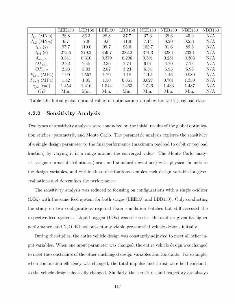
LEE150 LEB150 LBE150 LBB150 NEE150 NEB150 NBE150 NBB150It,1 (MN·s) 28.8 36.3 28.8 37.7 37.3 39.6 45.9 N/AIt,2 (MN·s) 6.7 7.9 9.6 11.9 7.14 9.20 9.251 N/Atb,1 (s) 97.7 110.0 99.7 95.6 102.7 91.6 89.6 N/Atb,2 (s) 273.6 379.3 359.7 382.2 374.3 328.1 233.1 N/Aδnozzle 0.341 0.310 0.379 0.296 0.301 0.281 0.303 N/AOFav,1 2.32 2.45 2.36 2.74 6.91 4.70 7.73 N/AOFav,2 2.93 3.03 2.87 3.23 6.34 5.93 6.96 N/A

Pup,1 (MPa) 1.00 1.552 1.20 1.18 1.12 1.46 0.989 N/APup,2 (MPa) 1.42 1.05 1.50 0.861 0.627 0.701 1.359 N/Aγpo (rad) 1.454 1.416 1.544 1.463 1.526 1.433 1.487 N/AOD Min. Min. Min. Min. Min. Min. Min. N/A

Table 4.6: Initial global optimal values of optimization variables for 150 kg payload class

4.2.2 Sensitivity Analysis

Two types of sensitivity analyses were conducted on the initial results of the global optimiza-

tion studies: parametric, and Monte Carlo. The parametric analysis explores the sensitivity

of a single design parameter to the final performance (maximum payload to orbit or payload

fraction) by varying it in a range around the converged value. The Monte Carlo analy-

sis assigns normal distributions (mean and standard deviations) with physical bounds to

the design variables, and within these distributions samples each design variable for given

evaluations and determines the performance.

The sensitivity analysis was reduced to focusing on configurations with a single oxidizer

(LOx) with the same feed system for both stages (LEE150 and LBB150). Only conducting

the study on two configurations required fewer simulation batches but still assessed the

respective feed systems. Liquid oxygen (LOx) was selected as the oxidizer given its higher

performance, and N2O did not present any viable pressure-fed vehicle designs initially.

During the studies, the entire vehicle design was constantly adjusted to meet all other in-

put variables. When one input parameter was changed, the entire vehicle design was changed

to meet the constraints of the other unchanged design variables and constants. For example,

when combustion efficiency was changed, the total impulse and thrust were held constant,

so the vehicle design physically changed. Similarly, the structures and trajectory are always

117

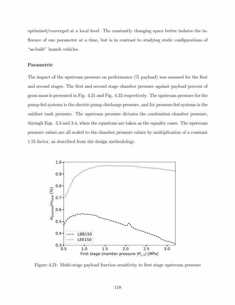
optimized/converged at a local level. The constantly changing space better isolates the in-

fluence of one parameter at a time, but is in contrast to studying static configurations of

“as-built” launch vehicles.

Parametric

The impact of the upstream pressure on performance (% payload) was assessed for the first

and second stages. The first and second stage chamber pressure against payload percent of

gross mass is presented in Fig. 4.21 and Fig. 4.22 respectively. The upstream pressure for the

pump-fed systems is the electric-pump discharge pressure, and for pressure-fed systems is the

oxidizer tank pressure. The upstream pressure dictates the combustion chamber pressure,

through Eqn. 3.3 and 3.4, when the equations are taken as the equality cases. The upstream

pressure values are all scaled to the chamber pressure values by multiplication of a constant

1.55 factor, as described from the design methodology.

0.5 1.0 1.5 2.0 2.5 3.0First stage chamber pressure (Pc, 1) [MPa]

0.3

0.4

0.5

0.6

0.7

0.8

0.9

1.0

mpa

yloa

d/mto

tal [

%]

LBB150LEE150

Figure 4.21: Multi-stage payload fraction sensitivity to first stage upstream pressure

118

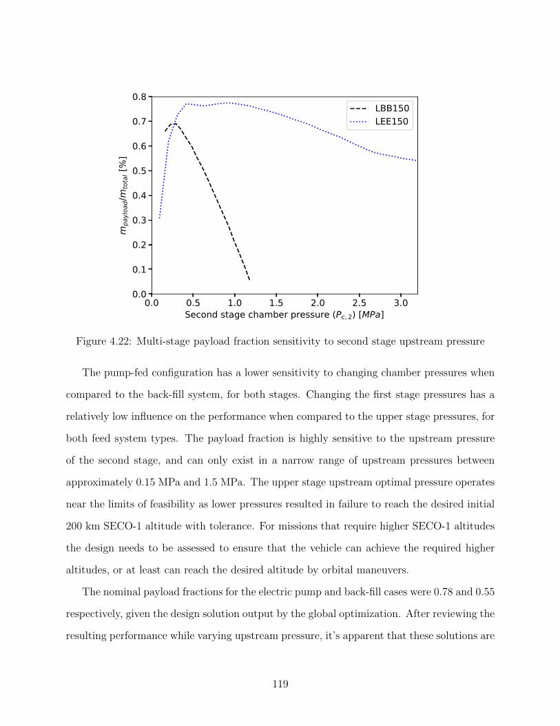
0.0 0.5 1.0 1.5 2.0 2.5 3.0Second stage chamber pressure (Pc, 2) [MPa]

0.0

0.1

0.2

0.3

0.4

0.5

0.6

0.7

0.8

mpa

yloa

d/mto

tal [

%]

LBB150LEE150

Figure 4.22: Multi-stage payload fraction sensitivity to second stage upstream pressure

The pump-fed configuration has a lower sensitivity to changing chamber pressures when

compared to the back-fill system, for both stages. Changing the first stage pressures has a

relatively low influence on the performance when compared to the upper stage pressures, for

both feed system types. The payload fraction is highly sensitive to the upstream pressure

of the second stage, and can only exist in a narrow range of upstream pressures between

approximately 0.15 MPa and 1.5 MPa. The upper stage upstream optimal pressure operates

near the limits of feasibility as lower pressures resulted in failure to reach the desired initial

200 km SECO-1 altitude with tolerance. For missions that require higher SECO-1 altitudes

the design needs to be assessed to ensure that the vehicle can achieve the required higher

altitudes, or at least can reach the desired altitude by orbital maneuvers.

The nominal payload fractions for the electric pump and back-fill cases were 0.78 and 0.55

respectively, given the design solution output by the global optimization. After reviewing the

resulting performance while varying upstream pressure, it’s apparent that these solutions are

119

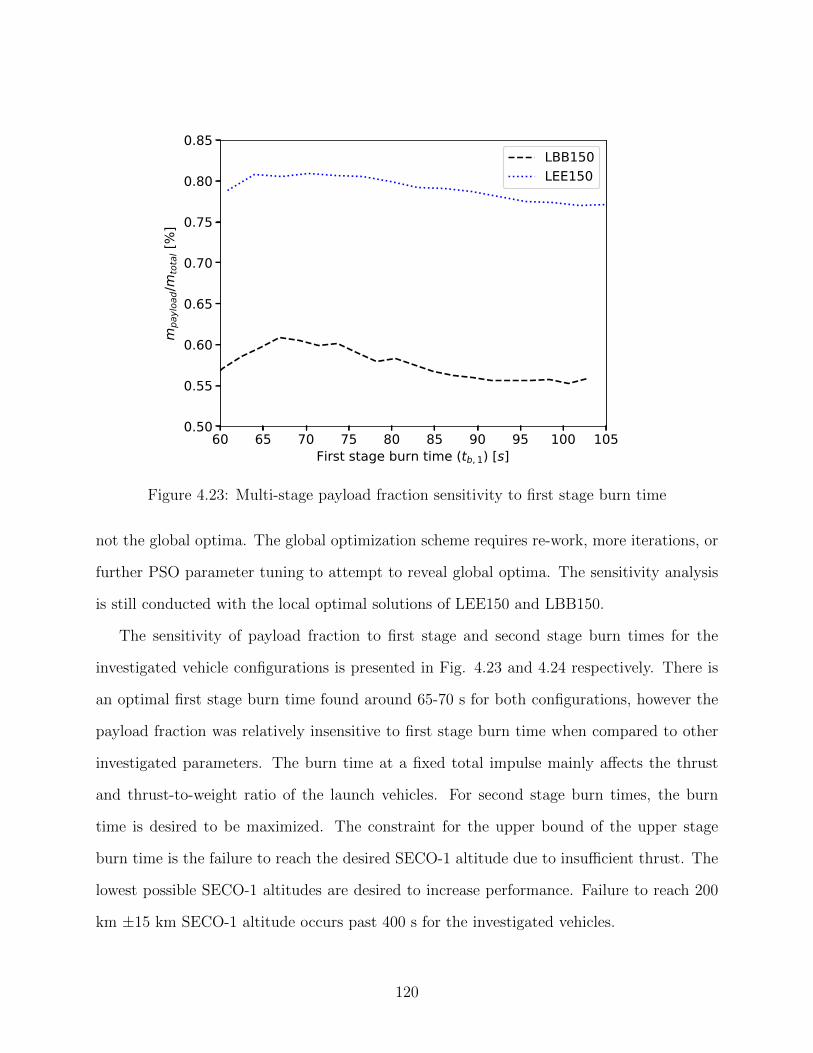
60 65 70 75 80 85 90 95 100 105First stage burn time (tb, 1) [s]

0.50

0.55

0.60

0.65

0.70

0.75

0.80

0.85

mpa

yloa

d/mto

tal [

%]

LBB150LEE150

Figure 4.23: Multi-stage payload fraction sensitivity to first stage burn time

not the global optima. The global optimization scheme requires re-work, more iterations, or

further PSO parameter tuning to attempt to reveal global optima. The sensitivity analysis

is still conducted with the local optimal solutions of LEE150 and LBB150.

The sensitivity of payload fraction to first stage and second stage burn times for the

investigated vehicle configurations is presented in Fig. 4.23 and 4.24 respectively. There is

an optimal first stage burn time found around 65-70 s for both configurations, however the

payload fraction was relatively insensitive to first stage burn time when compared to other

investigated parameters. The burn time at a fixed total impulse mainly affects the thrust

and thrust-to-weight ratio of the launch vehicles. For second stage burn times, the burn

time is desired to be maximized. The constraint for the upper bound of the upper stage

burn time is the failure to reach the desired SECO-1 altitude due to insufficient thrust. The

lowest possible SECO-1 altitudes are desired to increase performance. Failure to reach 200

km ±15 km SECO-1 altitude occurs past 400 s for the investigated vehicles.

120

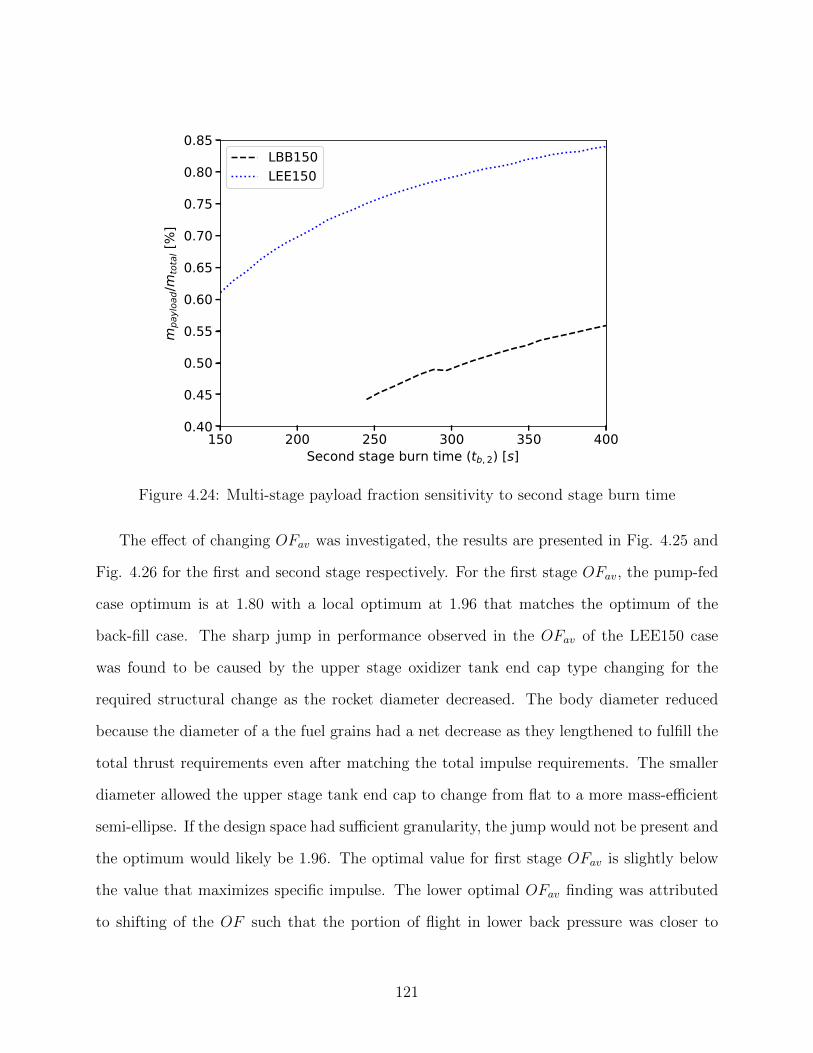
150 200 250 300 350 400Second stage burn time (tb, 2) [s]

0.40

0.45

0.50

0.55

0.60

0.65

0.70

0.75

0.80

0.85

mpa

yloa

d/mto

tal [

%]

LBB150LEE150

Figure 4.24: Multi-stage payload fraction sensitivity to second stage burn time

The effect of changing OFav was investigated, the results are presented in Fig. 4.25 and

Fig. 4.26 for the first and second stage respectively. For the first stage OFav, the pump-fed

case optimum is at 1.80 with a local optimum at 1.96 that matches the optimum of the

back-fill case. The sharp jump in performance observed in the OFav of the LEE150 case

was found to be caused by the upper stage oxidizer tank end cap type changing for the

required structural change as the rocket diameter decreased. The body diameter reduced

because the diameter of a the fuel grains had a net decrease as they lengthened to fulfill the

total thrust requirements even after matching the total impulse requirements. The smaller

diameter allowed the upper stage tank end cap to change from flat to a more mass-efficient

semi-ellipse. If the design space had sufficient granularity, the jump would not be present and

the optimum would likely be 1.96. The optimal value for first stage OFav is slightly below

the value that maximizes specific impulse. The lower optimal OFav finding was attributed

to shifting of the OF such that the portion of flight in lower back pressure was closer to

121

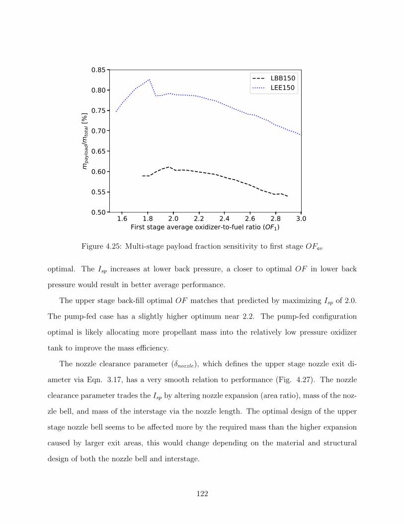
1.6 1.8 2.0 2.2 2.4 2.6 2.8 3.0First stage average oxidizer-to-fuel ratio (OF1)

0.50

0.55

0.60

0.65

0.70

0.75

0.80

0.85

mpa

yloa

d/mto

tal [

%]

LBB150LEE150

Figure 4.25: Multi-stage payload fraction sensitivity to first stage OFav

optimal. The Isp increases at lower back pressure, a closer to optimal OF in lower back

pressure would result in better average performance.

The upper stage back-fill optimal OF matches that predicted by maximizing Isp of 2.0.

The pump-fed case has a slightly higher optimum near 2.2. The pump-fed configuration

optimal is likely allocating more propellant mass into the relatively low pressure oxidizer

tank to improve the mass efficiency.

The nozzle clearance parameter (δnozzle), which defines the upper stage nozzle exit di-

ameter via Eqn. 3.17, has a very smooth relation to performance (Fig. 4.27). The nozzle

clearance parameter trades the Isp by altering nozzle expansion (area ratio), mass of the noz-

zle bell, and mass of the interstage via the nozzle length. The optimal design of the upper

stage nozzle bell seems to be affected more by the required mass than the higher expansion

caused by larger exit areas, this would change depending on the material and structural

design of both the nozzle bell and interstage.

122

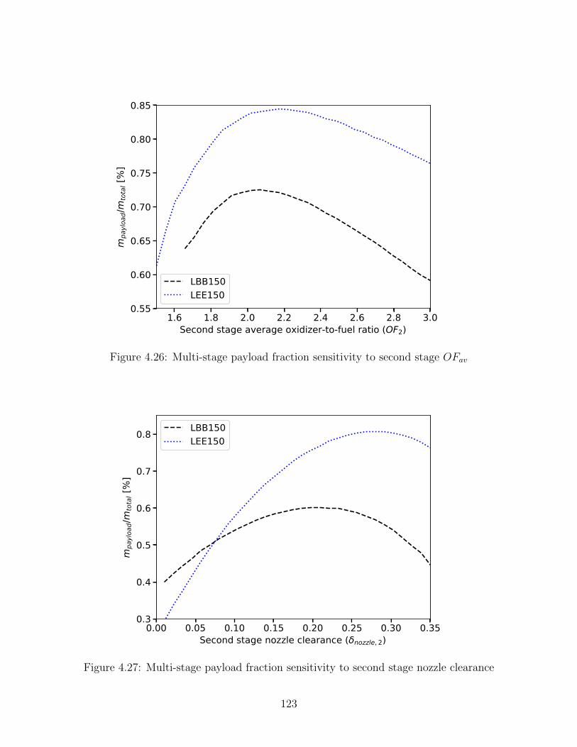
1.6 1.8 2.0 2.2 2.4 2.6 2.8 3.0Second stage average oxidizer-to-fuel ratio (OF2)

0.55

0.60

0.65

0.70

0.75

0.80

0.85m

payl

oad/m

tota

l [%

]

LBB150LEE150

Figure 4.26: Multi-stage payload fraction sensitivity to second stage OFav

0.00 0.05 0.10 0.15 0.20 0.25 0.30 0.35Second stage nozzle clearance ( nozzle, 2)

0.3

0.4

0.5

0.6

0.7

0.8

mpa

yloa

d/mto

tal [

%]

LBB150LEE150

Figure 4.27: Multi-stage payload fraction sensitivity to second stage nozzle clearance

123

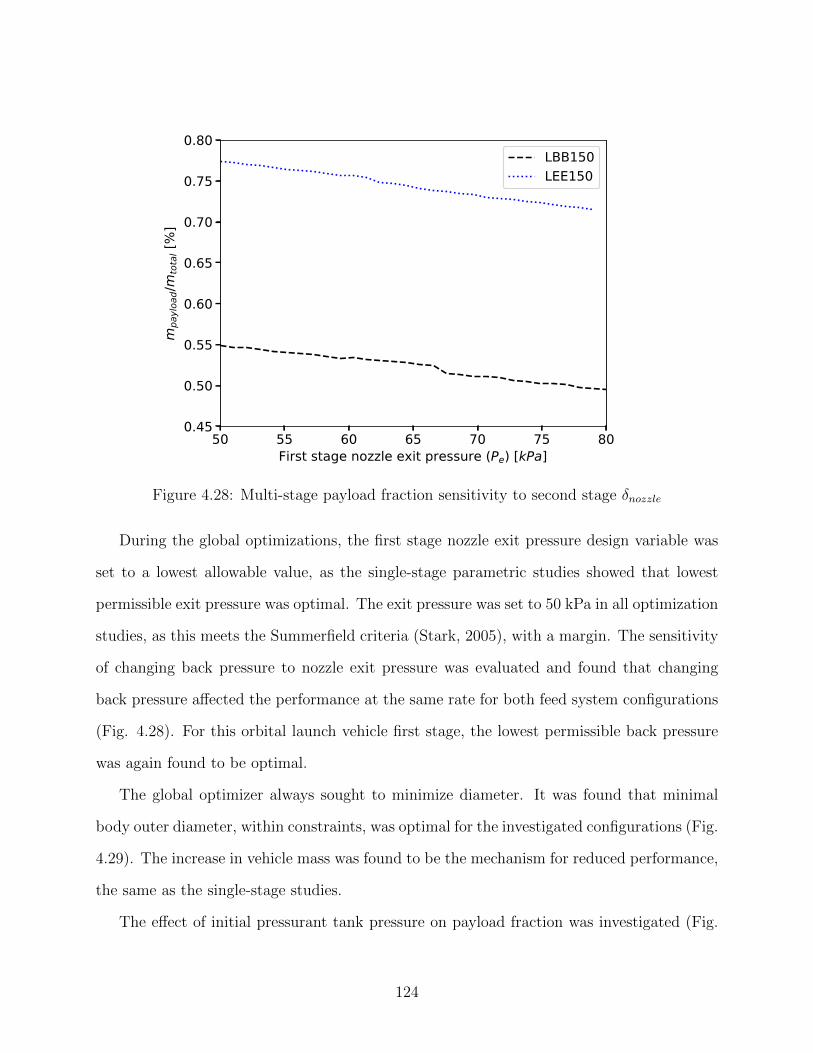
50 55 60 65 70 75 80First stage nozzle exit pressure (Pe) [kPa]

0.45

0.50

0.55

0.60

0.65

0.70

0.75

0.80

mpa

yloa

d/mto

tal [

%]

LBB150LEE150

Figure 4.28: Multi-stage payload fraction sensitivity to second stage δnozzle

During the global optimizations, the first stage nozzle exit pressure design variable was

set to a lowest allowable value, as the single-stage parametric studies showed that lowest

permissible exit pressure was optimal. The exit pressure was set to 50 kPa in all optimization

studies, as this meets the Summerfield criteria (Stark, 2005), with a margin. The sensitivity

of changing back pressure to nozzle exit pressure was evaluated and found that changing

back pressure affected the performance at the same rate for both feed system configurations

(Fig. 4.28). For this orbital launch vehicle first stage, the lowest permissible back pressure

was again found to be optimal.

The global optimizer always sought to minimize diameter. It was found that minimal

body outer diameter, within constraints, was optimal for the investigated configurations (Fig.

4.29). The increase in vehicle mass was found to be the mechanism for reduced performance,

the same as the single-stage studies.

The effect of initial pressurant tank pressure on payload fraction was investigated (Fig.

124

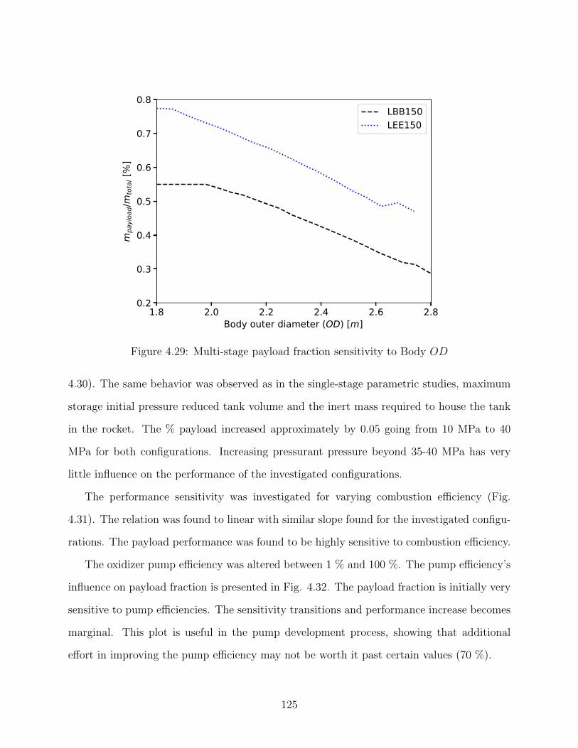
1.8 2.0 2.2 2.4 2.6 2.8Body outer diameter (OD) [m]

0.2

0.3

0.4

0.5

0.6

0.7

0.8

mpa

yloa

d/mto

tal [

%]

LBB150LEE150

Figure 4.29: Multi-stage payload fraction sensitivity to Body OD

4.30). The same behavior was observed as in the single-stage parametric studies, maximum

storage initial pressure reduced tank volume and the inert mass required to house the tank

in the rocket. The % payload increased approximately by 0.05 going from 10 MPa to 40

MPa for both configurations. Increasing pressurant pressure beyond 35-40 MPa has very

little influence on the performance of the investigated configurations.

The performance sensitivity was investigated for varying combustion efficiency (Fig.

4.31). The relation was found to linear with similar slope found for the investigated configu-

rations. The payload performance was found to be highly sensitive to combustion efficiency.

The oxidizer pump efficiency was altered between 1 % and 100 %. The pump efficiency’s

influence on payload fraction is presented in Fig. 4.32. The payload fraction is initially very

sensitive to pump efficiencies. The sensitivity transitions and performance increase becomes

marginal. This plot is useful in the pump development process, showing that additional

effort in improving the pump efficiency may not be worth it past certain values (70 %).

125

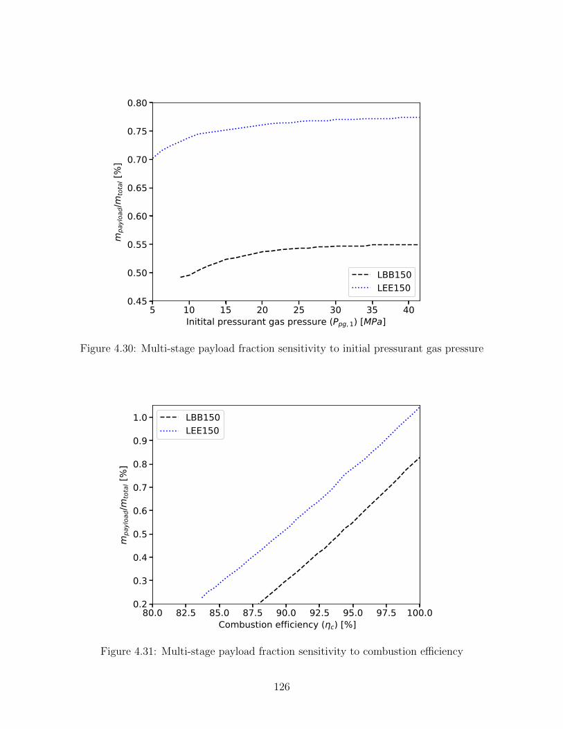
5 10 15 20 25 30 35 40Initital pressurant gas pressure (Ppg, 1) [MPa]

0.45

0.50

0.55

0.60

0.65

0.70

0.75

0.80m

payl

oad/m

tota

l [%

]

LBB150LEE150

Figure 4.30: Multi-stage payload fraction sensitivity to initial pressurant gas pressure

80.0 82.5 85.0 87.5 90.0 92.5 95.0 97.5 100.0 Combustion efficiency ( c) [%]

0.2

0.3

0.4

0.5

0.6

0.7

0.8

0.9

1.0

mpa

yloa

d/mto

tal [

%]

LBB150LEE150

Figure 4.31: Multi-stage payload fraction sensitivity to combustion efficiency

126

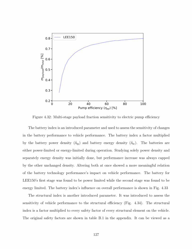
0 20 40 60 80 100Pump efficiency ( ep) [%]

0.2

0.3

0.4

0.5

0.6

0.7

0.8m

payl

oad/m

tota

l [%

]LEE150

Figure 4.32: Multi-stage payload fraction sensitivity to electric pump efficiency

The battery index is an introduced parameter and used to assess the sensitivity of changes

in the battery performance to vehicle performance. The battery index a factor multiplied

by the battery power density (δbp) and battery energy density (δbe). The batteries are

either power-limited or energy-limited during operation. Studying solely power density and

separately energy density was initially done, but performance increase was always capped

by the other unchanged density. Altering both at once showed a more meaningful relation

of the battery technology performance’s impact on vehicle performance. The battery for

LEE150’s first stage was found to be power limited while the second stage was found to be

energy limited. The battery index’s influence on overall performance is shown in Fig. 4.33

The structural index is another introduced parameter. It was introduced to assess the

sensitivity of vehicle performance to the structural efficiency (Fig. 4.34). The structural

index is a factor multiplied to every safety factor of every structural element on the vehicle.

The original safety factors are shown in table B.1 in the appendix. It can be viewed as a

127

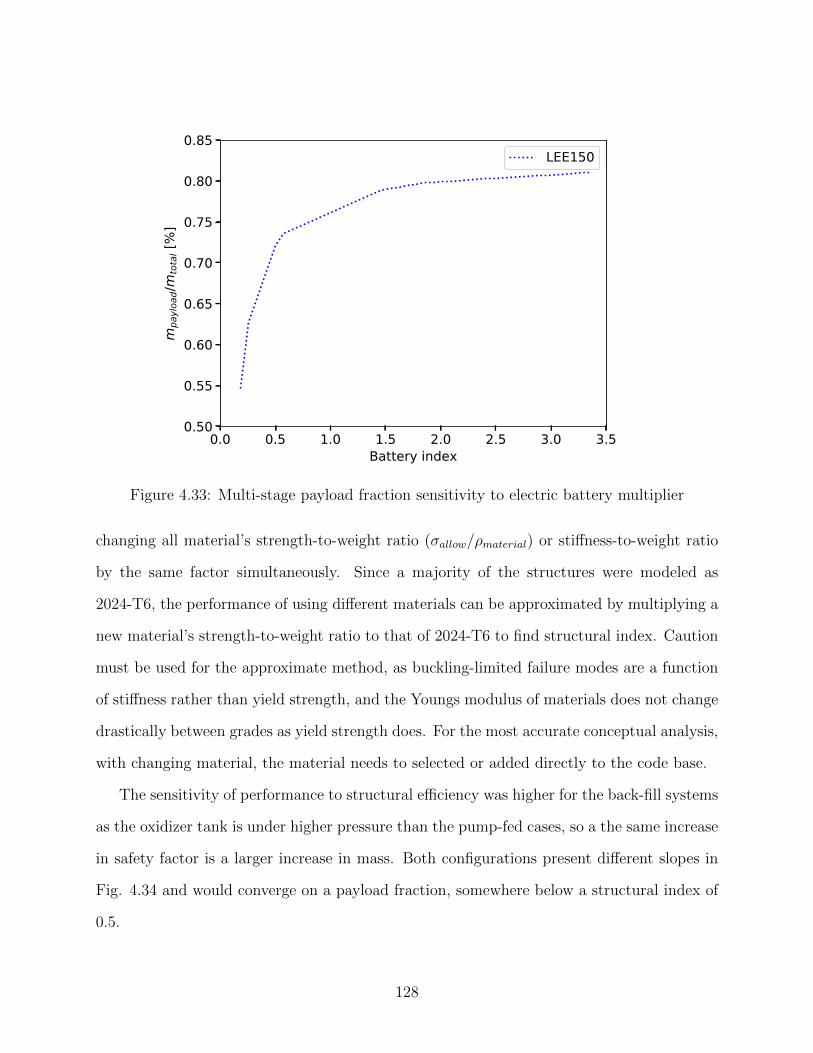
0.0 0.5 1.0 1.5 2.0 2.5 3.0 3.5Battery index

0.50

0.55

0.60

0.65

0.70

0.75

0.80

0.85

mpa

yloa

d/mto

tal [

%]

LEE150

Figure 4.33: Multi-stage payload fraction sensitivity to electric battery multiplier

changing all material’s strength-to-weight ratio (σallow/ρmaterial) or stiffness-to-weight ratio

by the same factor simultaneously. Since a majority of the structures were modeled as

2024-T6, the performance of using different materials can be approximated by multiplying a

new material’s strength-to-weight ratio to that of 2024-T6 to find structural index. Caution

must be used for the approximate method, as buckling-limited failure modes are a function

of stiffness rather than yield strength, and the Youngs modulus of materials does not change

drastically between grades as yield strength does. For the most accurate conceptual analysis,

with changing material, the material needs to selected or added directly to the code base.

The sensitivity of performance to structural efficiency was higher for the back-fill systems

as the oxidizer tank is under higher pressure than the pump-fed cases, so a the same increase

in safety factor is a larger increase in mass. Both configurations present different slopes in

Fig. 4.34 and would converge on a payload fraction, somewhere below a structural index of

0.5.

128

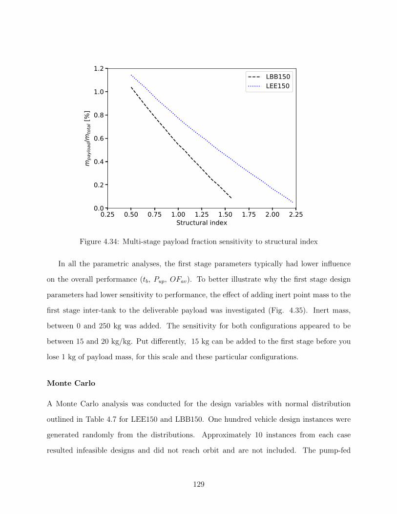
0.25 0.50 0.75 1.00 1.25 1.50 1.75 2.00 2.25Structural index

0.0

0.2

0.4

0.6

0.8

1.0

1.2

mpa

yloa

d/mto

tal [

%]

LBB150LEE150

Figure 4.34: Multi-stage payload fraction sensitivity to structural index

In all the parametric analyses, the first stage parameters typically had lower influence

on the overall performance (tb, Pup, OFav). To better illustrate why the first stage design

parameters had lower sensitivity to performance, the effect of adding inert point mass to the

first stage inter-tank to the deliverable payload was investigated (Fig. 4.35). Inert mass,

between 0 and 250 kg was added. The sensitivity for both configurations appeared to be

between 15 and 20 kg/kg. Put differently, 15 kg can be added to the first stage before you

lose 1 kg of payload mass, for this scale and these particular configurations.

Monte Carlo

A Monte Carlo analysis was conducted for the design variables with normal distribution

outlined in Table 4.7 for LEE150 and LBB150. One hundred vehicle design instances were

generated randomly from the distributions. Approximately 10 instances from each case

resulted infeasible designs and did not reach orbit and are not included. The pump-fed

129

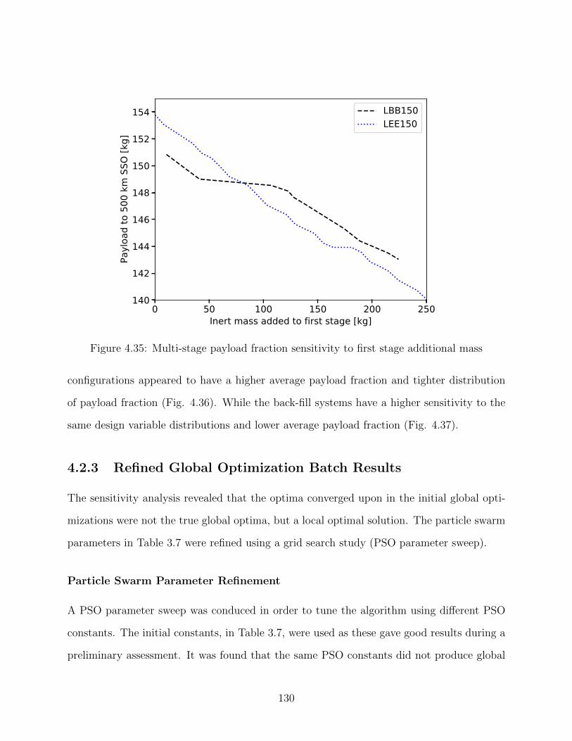
0 50 100 150 200 250Inert mass added to first stage [kg]

140

142

144

146

148

150

152

154Pa

yloa

d to

500

km

SSO

[kg]

LBB150LEE150

Figure 4.35: Multi-stage payload fraction sensitivity to first stage additional mass

configurations appeared to have a higher average payload fraction and tighter distribution

of payload fraction (Fig. 4.36). While the back-fill systems have a higher sensitivity to the

same design variable distributions and lower average payload fraction (Fig. 4.37).

4.2.3 Refined Global Optimization Batch Results

The sensitivity analysis revealed that the optima converged upon in the initial global opti-

mizations were not the true global optima, but a local optimal solution. The particle swarm

parameters in Table 3.7 were refined using a grid search study (PSO parameter sweep).

Particle Swarm Parameter Refinement

A PSO parameter sweep was conduced in order to tune the algorithm using different PSO

constants. The initial constants, in Table 3.7, were used as these gave good results during a

preliminary assessment. It was found that the same PSO constants did not produce global

130

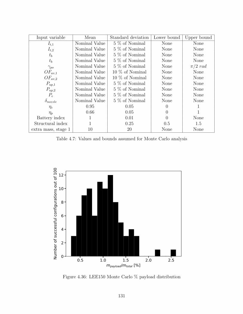
Input variable Mean Standard deviation Lower bound Upper boundIt,1 Nominal Value 5 % of Nominal None NoneIt,2 Nominal Value 5 % of Nominal None Nonetb Nominal Value 5 % of Nominal None Nonetb Nominal Value 5 % of Nominal None Noneγpo Nominal Value 5 % of Nominal None π/2 rad

OFav,1 Nominal Value 10 % of Nominal None NoneOFav,2 Nominal Value 10 % of Nominal None NonePup,1 Nominal Value 5 % of Nominal None NonePup,2 Nominal Value 5 % of Nominal None NonePe Nominal Value 5 % of Nominal None None

δnozzle Nominal Value 5 % of Nominal None Noneηc 0.95 0.05 0 1ηp 0.66 0.05 0 1

Battery index 1 0.01 0 NoneStructural index 1 0.25 0.5 1.5

extra mass, stage 1 10 20 None None

Table 4.7: Values and bounds assumed for Monte Carlo analysis

0.5 1.0 1.5 2.0 2.5mpayload/mtotal [%]

0

2

4

6

8

10

12

Num

ber o

f suc

cess

ful c

onfig

urat

ions

out

of 1

00

Figure 4.36: LEE150 Monte Carlo % payload distribution

131

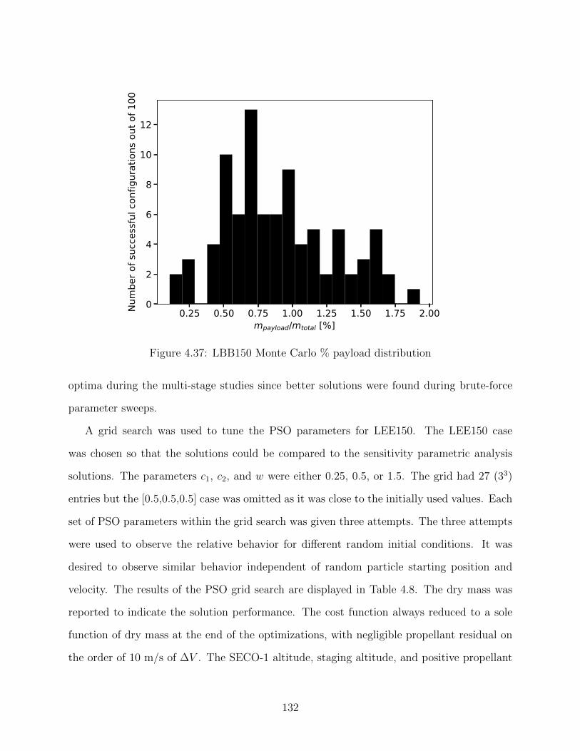
0.25 0.50 0.75 1.00 1.25 1.50 1.75 2.00mpayload/mtotal [%]

0

2

4

6

8

10

12Nu

mbe

r of s

ucce

ssfu

l con

figur

atio

ns o

ut o

f 100

Figure 4.37: LBB150 Monte Carlo % payload distribution

optima during the multi-stage studies since better solutions were found during brute-force

parameter sweeps.

A grid search was used to tune the PSO parameters for LEE150. The LEE150 case

was chosen so that the solutions could be compared to the sensitivity parametric analysis

solutions. The parameters c1, c2, and w were either 0.25, 0.5, or 1.5. The grid had 27 (33)

entries but the [0.5,0.5,0.5] case was omitted as it was close to the initially used values. Each

set of PSO parameters within the grid search was given three attempts. The three attempts

were used to observe the relative behavior for different random initial conditions. It was

desired to observe similar behavior independent of random particle starting position and

velocity. The results of the PSO grid search are displayed in Table 4.8. The dry mass was

reported to indicate the solution performance. The cost function always reduced to a sole

function of dry mass at the end of the optimizations, with negligible propellant residual on

the order of 10 m/s of ∆V . The SECO-1 altitude, staging altitude, and positive propellant

132

remainder error weights were sized to be sufficiently large so that they were never violated

in the final solution. The dry masses in Table 4.8 can be converted to cost function values

by multiplying by 100. It was found that weighting the social and cognitive parameters

relatively high with a lower particle mass resulted in the best consistency between attempts

as well as very good global solutions. The payload fractions that were a result of the best

global solutions surpassed the maximum encountered in the parametric analysis (when only

considering the optimization variables). The highest payload fraction for LEE150 in the

global optimization was 1.20 % while the highest found during the sensitivity analysis was

0.97 %, when only considering the optimizable variables. The 0.97 % payload for LEE150

was initially found during the first stage upstream pressure parametric sensitivity analysis.

Solutions using [c1:1.5, c2:1.5 w:0.25] found the minimum dry mass of the a LEE150 case

to be 1350 kg, within a 100 kg window for three attempts, and the best was within 10 kg

dry mass of the overall best. The overall best was found using [c1:0.5, c2:1.5 w:0.5] but

was not reliably found from the other attempts for the same PSO parameters. The PSO

parameters: [c1:1.5, c2:1.5 w:0.25] showed the most promise and were used going forward. If

time permitted, further refinement of the PSO parameters would be investigated with lower

particle mass and higher cognitive and social constants.

The best cost function of a generation, for the [c1:1.5, c2:1.5 w:0.25] LEE150 cases, for

each iteration number is plotted in Fig. 4.38. The plot is a result of three independent

concurrent global optimization runs. All three runs converged to within a 100 kg window

for the vehicle dry mass. The plot presents more noise than the previous convergence plot

(Fig. 4.20). The noise is a result of the higher acceleration and sporadic particle movement.

It was initially thought that higher particle weight (inertia) would prevent local optimal

convergence, but that was not observed.

133

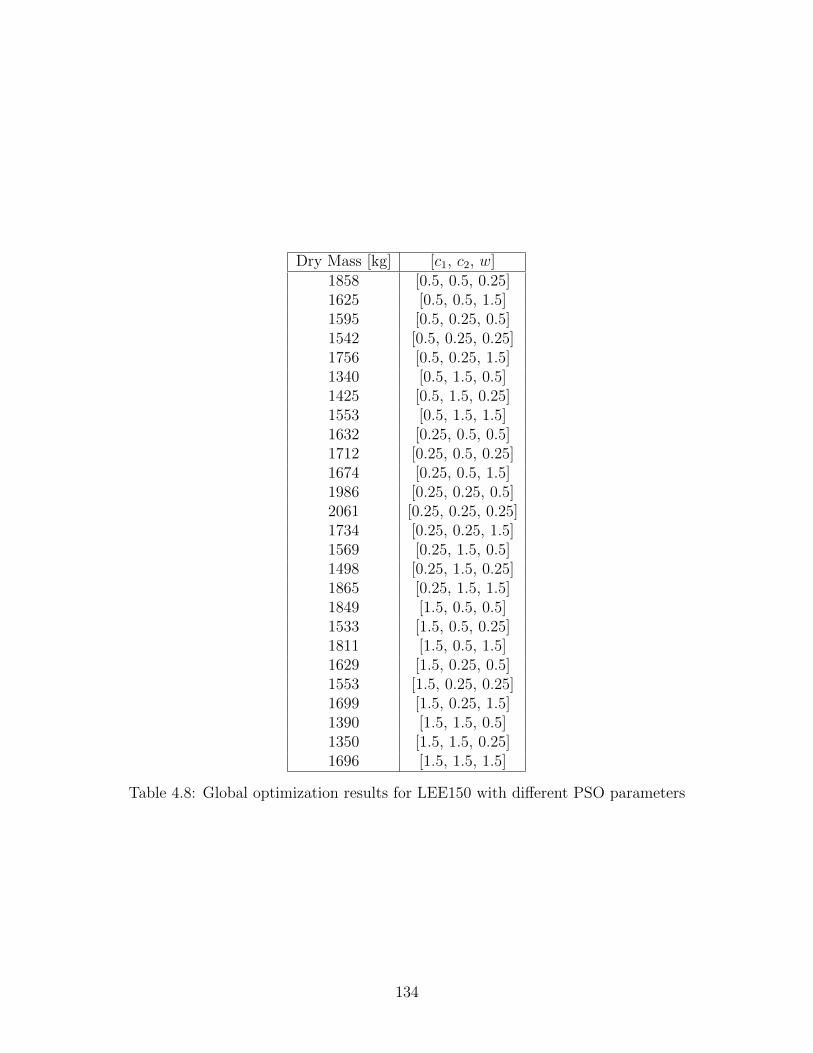
Dry Mass [kg] [c1, c2, w]1858 [0.5, 0.5, 0.25]1625 [0.5, 0.5, 1.5]1595 [0.5, 0.25, 0.5]1542 [0.5, 0.25, 0.25]1756 [0.5, 0.25, 1.5]1340 [0.5, 1.5, 0.5]1425 [0.5, 1.5, 0.25]1553 [0.5, 1.5, 1.5]1632 [0.25, 0.5, 0.5]1712 [0.25, 0.5, 0.25]1674 [0.25, 0.5, 1.5]1986 [0.25, 0.25, 0.5]2061 [0.25, 0.25, 0.25]1734 [0.25, 0.25, 1.5]1569 [0.25, 1.5, 0.5]1498 [0.25, 1.5, 0.25]1865 [0.25, 1.5, 1.5]1849 [1.5, 0.5, 0.5]1533 [1.5, 0.5, 0.25]1811 [1.5, 0.5, 1.5]1629 [1.5, 0.25, 0.5]1553 [1.5, 0.25, 0.25]1699 [1.5, 0.25, 1.5]1390 [1.5, 1.5, 0.5]1350 [1.5, 1.5, 0.25]1696 [1.5, 1.5, 1.5]

Table 4.8: Global optimization results for LEE150 with different PSO parameters

134

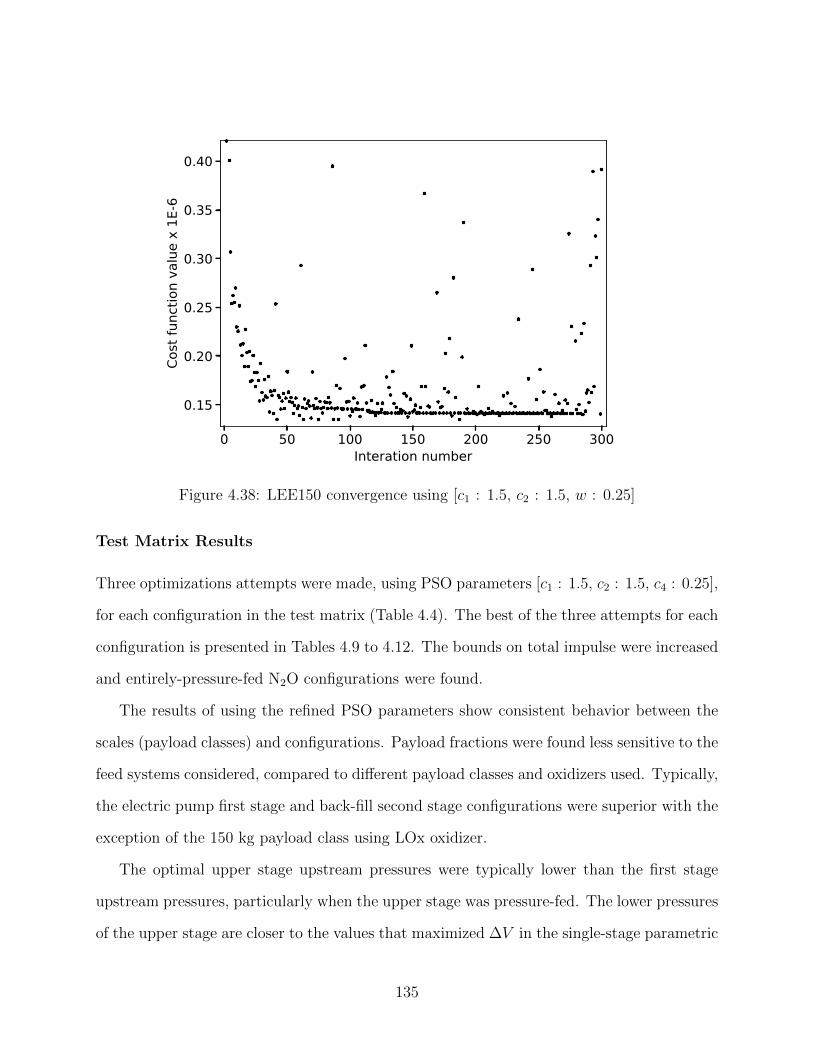
0 50 100 150 200 250 300Interation number

0.15

0.20

0.25

0.30

0.35

0.40Co

st fu

nctio

n va

lue

x 1E

-6

Figure 4.38: LEE150 convergence using [c1 : 1.5, c2 : 1.5, w : 0.25]

Test Matrix Results

Three optimizations attempts were made, using PSO parameters [c1 : 1.5, c2 : 1.5, c4 : 0.25],

for each configuration in the test matrix (Table 4.4). The best of the three attempts for each

configuration is presented in Tables 4.9 to 4.12. The bounds on total impulse were increased

and entirely-pressure-fed N2O configurations were found.

The results of using the refined PSO parameters show consistent behavior between the

scales (payload classes) and configurations. Payload fractions were found less sensitive to the

feed systems considered, compared to different payload classes and oxidizers used. Typically,

the electric pump first stage and back-fill second stage configurations were superior with the

exception of the 150 kg payload class using LOx oxidizer.

The optimal upper stage upstream pressures were typically lower than the first stage

upstream pressures, particularly when the upper stage was pressure-fed. The lower pressures

of the upper stage are closer to the values that maximized ∆V in the single-stage parametric

135

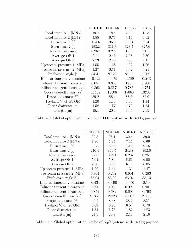
LEE150 LEB150 LBE150 LBB150Total impulse 1 [MN·s] 19.7 18.4 22.3 18.3Total impulse 2 [MN·s] 4.55 6.76 4.16 6.02

Burn time 1 [s] 114.6 96.0 108.4 85.4Burn time 2 [s] 493.2 316.3 323.5 327.6

Nozzle clearance 0.287 0.222 0.285 0.151Average OF 1 2.11 2.43 2.08 2.30Average OF 2 2.73 2.49 2.35 2.45

Upstream pressure 1 [MPa] 1.55 1.28 1.02 1.26Upstream pressure 2 [MPa] 1.27 0.51 1.02 0.21

Pitch-over angle [◦] 84.41 87.25 88.05 83.02Bilinear tangent χ constant -0.422 -0.479 -0.529 -0.543Bilinear tangent c constant 0.651 0.833 0.906 0.908Bilinear tangent b constant 0.862 0.817 0.782 0.774

Gross take-off mass [kg] 12488 13308 15060 13205Propellant mass [%] 89.2 88.4 88.6 86.9

Paylaod % of GTOM 1.20 1.13 1.00 1.14Outer diameter [m] 1.58 1.57 1.70 1.54

Length [m] 18.1 20.4 19.5 20.9

Table 4.9: Global optimization results of LOx systems with 150 kg payload

NEE150 NEB150 NBE150 NBB150Total impulse 1 [MN·s] 30.3 28.1 32.4 30.0Total impulse 2 [MN·s] 7.30 5.94 7.15 6.69

Burn time 1 [s] 92.3 80.6 72.9 94.6Burn time 2 [s] 210.9 364.5 242.8 392.0

Nozzle clearance 0.273 0.241 0.237 0.251Average OF 1 5.64 5.80 5.61 6.00Average OF 2 7.30 6.68 6.16 6.05

Upstream pressure 1 [MPa] 1.29 1.44 1.31 1.47Upstream pressure 2 [MPa] 0.864 0.202 0.651 0.283

Pitch-over angle [◦] 86.04 83.00 86.04 85.13Bilinear tangent χ constant -0.434 -0.690 -0.656 -0.503Bilinear tangent c constant 0.690 0.935 0.928 0.901Bilinear tangent b constant 0.852 0.682 0.699 0.798

Gross take-off mass [kg] 21850 19723 23507 21465Propellant mass [%] 90.2 89.8 88.2 88.1

Paylaod % of GTOM 0.69 0.76 0.64 0.70Outer diameter [m] 1.84 1.76 1.82 1.83

Length [m] 21.3 20.8 22.7 21.6

Table 4.10: Global optimization results of N2O systems with 150 kg payload

136

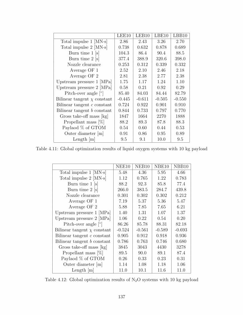
LEE10 LEB10 LBE10 LBB10Total impulse 1 [MN·s] 2.86 2.43 3.26 2.70Total impulse 2 [MN·s] 0.738 0.632 0.878 0.689

Burn time 1 [s] 104.3 86.4 90.4 88.5Burn time 2 [s] 377.4 388.9 320.6 398.0

Nozzle clearance 0.253 0.312 0.339 0.332Average OF 1 2.52 2.10 2.46 2.18Average OF 2 2.81 2.38 2.77 2.38

Upstream pressure 1 [MPa] 1.75 1.17 1.24 1.10Upstream pressure 2 [MPa] 0.58 0.21 0.92 0.29

Pitch-over angle [◦] 85.40 84.03 84.44 82.79Bilinear tangent χ constant -0.445 -0.611 -0.505 -0.550Bilinear tangent c constant 0.724 0.922 0.901 0.910Bilinear tangent b constant 0.844 0.733 0.797 0.770

Gross take-off mass [kg] 1847 1664 2270 1888Propellant mass [%] 88.2 89.3 87.8 88.3

Paylaod % of GTOM 0.54 0.60 0.44 0.53Outer diameter [m] 0.91 0.86 0.95 0.89

Length [m] 9.5 9.1 10.0 9.5

Table 4.11: Global optimization results of liquid oxygen systems with 10 kg payload

NEE10 NEB10 NBE10 NBB10Total impulse 1 [MN·s] 5.48 4.36 5.95 4.66Total impulse 2 [MN·s] 1.12 0.765 1.22 0.783

Burn time 1 [s] 88.2 92.3 85.8 77.4Burn time 2 [s] 266.0 383.5 284.7 439.8

Nozzle clearance 0.301 0.302 0.302 0.212Average OF 1 7.19 5.37 5.36 5.47Average OF 2 5.88 7.85 7.65 6.21

Upstream pressure 1 [MPa] 1.40 1.31 1.07 1.37Upstream pressure 2 [MPa] 1.06 0.22 0.54 0.20

Pitch-over angle [◦] 86.26 85.78 88.31 82.18Bilinear tangent χ constant -0.524 -0.561 -0.589 -0.693Bilinear tangent c constant 0.905 0.912 0.918 0.936Bilinear tangent b constant 0.786 0.763 0.746 0.680

Gross take-off mass [kg] 3845 3043 4430 3278Propellant mass [%] 89.5 90.0 89.1 87.4

Paylaod % of GTOM 0.26 0.33 0.23 0.31Outer diameter [m] 1.14 1.08 1.18 1.06

Length [m] 11.0 10.1 11.6 11.0

Table 4.12: Global optimization results of N2O systems with 10 kg payload

137

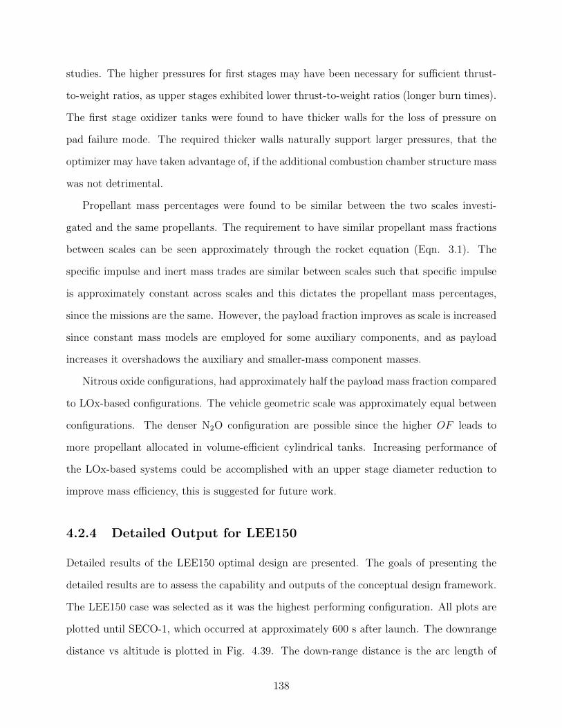
studies. The higher pressures for first stages may have been necessary for sufficient thrust-

to-weight ratios, as upper stages exhibited lower thrust-to-weight ratios (longer burn times).

The first stage oxidizer tanks were found to have thicker walls for the loss of pressure on

pad failure mode. The required thicker walls naturally support larger pressures, that the

optimizer may have taken advantage of, if the additional combustion chamber structure mass

was not detrimental.

Propellant mass percentages were found to be similar between the two scales investi-

gated and the same propellants. The requirement to have similar propellant mass fractions

between scales can be seen approximately through the rocket equation (Eqn. 3.1). The

specific impulse and inert mass trades are similar between scales such that specific impulse

is approximately constant across scales and this dictates the propellant mass percentages,

since the missions are the same. However, the payload fraction improves as scale is increased

since constant mass models are employed for some auxiliary components, and as payload

increases it overshadows the auxiliary and smaller-mass component masses.

Nitrous oxide configurations, had approximately half the payload mass fraction compared

to LOx-based configurations. The vehicle geometric scale was approximately equal between

configurations. The denser N2O configuration are possible since the higher OF leads to

more propellant allocated in volume-efficient cylindrical tanks. Increasing performance of

the LOx-based systems could be accomplished with an upper stage diameter reduction to

improve mass efficiency, this is suggested for future work.

4.2.4 Detailed Output for LEE150

Detailed results of the LEE150 optimal design are presented. The goals of presenting the

detailed results are to assess the capability and outputs of the conceptual design framework.

The LEE150 case was selected as it was the highest performing configuration. All plots are

plotted until SECO-1, which occurred at approximately 600 s after launch. The downrange

distance vs altitude is plotted in Fig. 4.39. The down-range distance is the arc length of

138

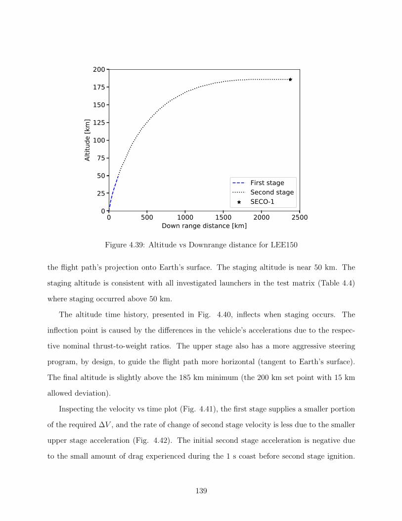
0 500 1000 1500 2000 2500Down range distance [km]

0

25

50

75

100

125

150

175

200

Altit

ude

[km

]

First stageSecond stageSECO-1

Figure 4.39: Altitude vs Downrange distance for LEE150

the flight path’s projection onto Earth’s surface. The staging altitude is near 50 km. The

staging altitude is consistent with all investigated launchers in the test matrix (Table 4.4)

where staging occurred above 50 km.

The altitude time history, presented in Fig. 4.40, inflects when staging occurs. The

inflection point is caused by the differences in the vehicle’s accelerations due to the respec-

tive nominal thrust-to-weight ratios. The upper stage also has a more aggressive steering

program, by design, to guide the flight path more horizontal (tangent to Earth’s surface).

The final altitude is slightly above the 185 km minimum (the 200 km set point with 15 km

allowed deviation).

Inspecting the velocity vs time plot (Fig. 4.41), the first stage supplies a smaller portion

of the required ∆V , and the rate of change of second stage velocity is less due to the smaller

upper stage acceleration (Fig. 4.42). The initial second stage acceleration is negative due

to the small amount of drag experienced during the 1 s coast before second stage ignition.

139

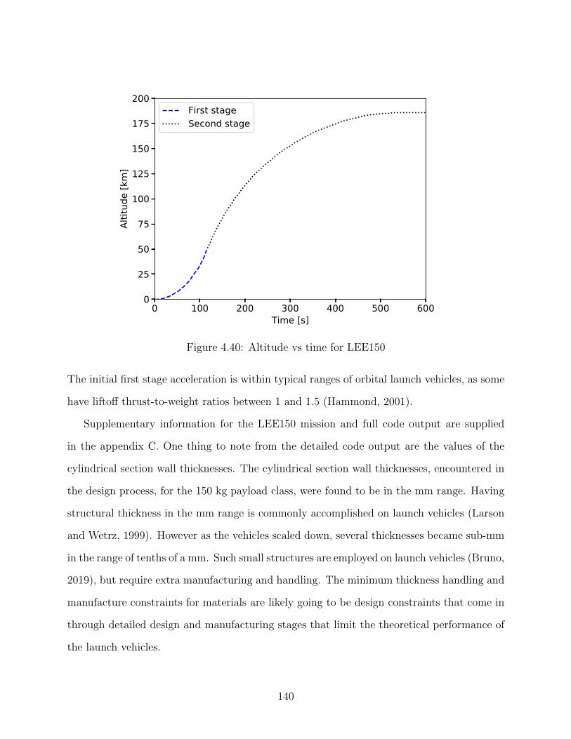
0 100 200 300 400 500 600Time [s]

0

25

50

75

100

125

150

175

200

Altit

ude

[km

]First stageSecond stage

Figure 4.40: Altitude vs time for LEE150

The initial first stage acceleration is within typical ranges of orbital launch vehicles, as some

have liftoff thrust-to-weight ratios between 1 and 1.5 (Hammond, 2001).

Supplementary information for the LEE150 mission and full code output are supplied

in the appendix C. One thing to note from the detailed code output are the values of the

cylindrical section wall thicknesses. The cylindrical section wall thicknesses, encountered in

the design process, for the 150 kg payload class, were found to be in the mm range. Having

structural thickness in the mm range is commonly accomplished on launch vehicles (Larson

and Wetrz, 1999). However as the vehicles scaled down, several thicknesses became sub-mm

in the range of tenths of a mm. Such small structures are employed on launch vehicles (Bruno,

2019), but require extra manufacturing and handling. The minimum thickness handling and

manufacture constraints for materials are likely going to be design constraints that come in

through detailed design and manufacturing stages that limit the theoretical performance of

the launch vehicles.

140

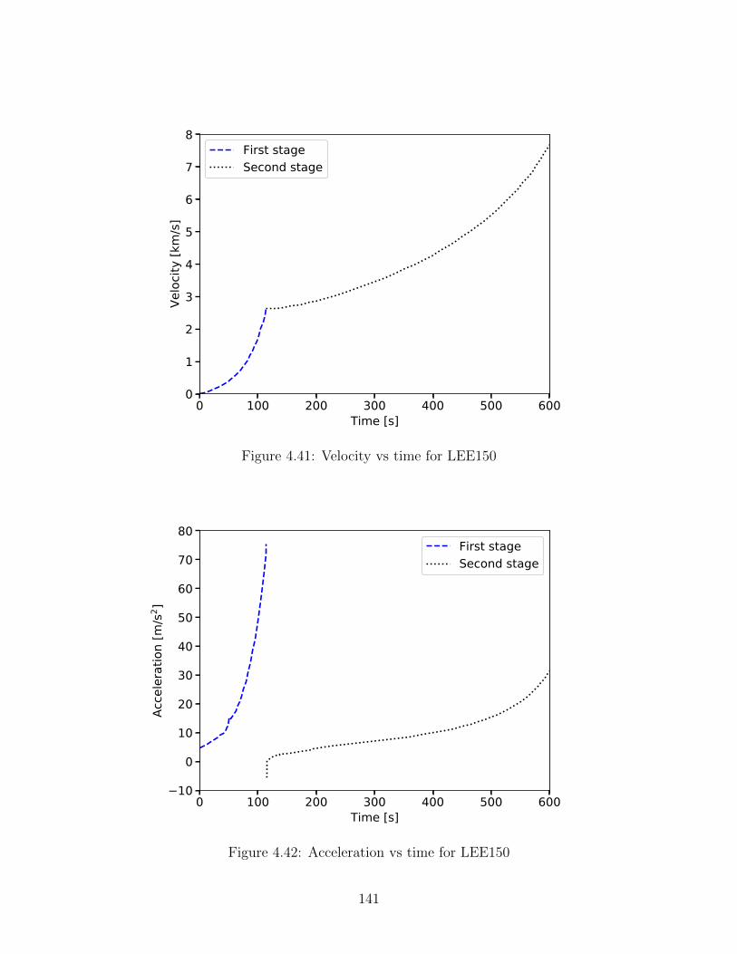
0 100 200 300 400 500 600Time [s]

0

1

2

3

4

5

6

7

8

Velo

city

[km

/s]

First stageSecond stage

Figure 4.41: Velocity vs time for LEE150

0 100 200 300 400 500 600Time [s]

10

0

10

20

30

40

50

60

70

80

Acce

lera

tion

[m/s

2 ]

First stageSecond stage

Figure 4.42: Acceleration vs time for LEE150

141

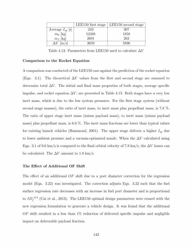
LEE150 first stage LEE150 second stageAverage Isp [s] 243 307

m0 [kg] 12488 1858mf [kg] 2691 262

∆V [m/s] 3659 5896

Table 4.13: Parameters from LEE150 used to calculate ∆V

Comparison to the Rocket Equation

A comparison was conducted of the LEE150 case against the prediction of the rocket equation

(Eqn. 3.1). The theoretical ∆V values from the first and second stage are summed to

determine total ∆V . The initial and final mass properties of both stages, average specific

impulse, and rocket equation ∆V , are presented in Table 4.13. Both stages have a very low

inert mass, which is due to the low system pressures. For the first stage system (without

second stage masses), the ratio of inert mass, to inert mass plus propellant mass, is 7.8 %.

The ratio of upper stage inert mass (minus payload mass), to inert mass (minus payload

mass) plus propellant mass, is 6.6 %. The inert mass fractions are lower than typical values

for existing launch vehicles (Hammond, 2001). The upper stage delivers a higher Isp due

to lower ambient pressure and a vacuum-optimized nozzle. When the ∆V calculated using

Eqn. 3.1 of 9.6 km/s is compared to the final orbital velocity of 7.8 km/s, the ∆V losses can

be calculated. The ∆V amount to 1.8 km/s.

The Effect of Additional OF Shift

The effect of an additional OF shift due to a port diameter correction for the regression

model (Eqn. 3.22) was investigated. The correction adjusts Eqn. 3.22 such that the fuel

surface regression rate decreases with an increase in fuel port diameter and is proportional

to ID−0.2f (Cai et al., 2013). The LEE150 optimal design parameters were reused with the

new regression formulation to generate a vehicle design. It was found that the additional

OF shift resulted in a less than 1% reduction of delivered specific impulse and negligible

impact on deliverable payload fraction.

142

Chapter 5

Conclusions and Recommendations

5.1 Conclusions

This study found that two-stage payload delivery to low Earth orbit was conceptually fea-

sible for hybrid rocket propelled electric pump-fed and pressure-fed vehicles using either

N2O/paraffin or LOx/paraffin propellants. Entirely back-fill-pressure-fed systems were found

to have conceptual design solutions for two-stage-to-orbit payload delivery. The performance

of the electric-pump feed system configurations was found to be relatively insensitive to tech-

nological improvements beyond the values used from current literature. The pressure-fed

configurations had comparable payload fractions to pump-fed configurations. The finding of

feasible two-stage pressure-fed designs was surprising, as the inert mass was expected to be

too high and Miranda (2015) found no feasible solutions.

Design variables were found where the optima occurred on extreme ends. For optima at

extreme ends, limiting bounds were chosen from design constraints and practical limits. For

variables that exhibited mid-range optimal solutions, a tuned global particle swarm opti-

mization algorithm found high-performing design solutions that traded all multi-disciplinary

design variables in the reduction of dry vehicle mass for a given payload mass. It was found

that the upper stages were most sensitive to all design variables compared to first stages.

143

The effects of additional inert mass or propulsion system efficiency is directly impacting the

performance of second stage/ payload mass.

The main research question of this thesis was to what extent can orbital-class HRE-based

launchers be scaled down? The minimum mass configurations were found with LOx-based

systems compared to N2O-based systems of the same payload class. However the geometric

size of the vehicle was approximately the same between N2O and LOx systems, N2O systems

were denser. Payload fractions improved, across the different configurations, as the vehicle

became larger to support larger payloads. The smallest gross vehicle mass, found for the

150 kg mission, was 12488 kg for a dual electric pump LOx/paraffin system. For the 10 kg

payload class, the minimum wet mass was found to be 1664 kg for LOx/paraffin system with

an electric pump-fed first stage and back-fill-pressure-fed stage second stage.

5.2 Future Work

A possible area of future work is the analysis of hybrid rockets using different engine cycles.

The first-stage performance could be improved by incorporating an air-breathing aspect.

The various engine cycles, integrated with vehicle design, could greatly improve the vehicle

performance. The improved performance may bring down vehicle size and complexity or

offer enough margins for, at least first stage, landing and re-use. Recent work, found in this

thesis’s literature review, have explored fully or partially reusable launch vehicle conceptual

design. Re-use of hybrid rockets is an area not found in the literature surveyed for this work.

A possible addition to modeling is including the effects of throttling the oxidizer flow rate.

Throttling may further optimize vehicle performance, as limiting max q and/or maximum

acceleration would reduce aerodynamic loads and inert mass while trading-off propulsive

performance. This was suggested by Miranda (2015) but was not explored here.

Other modeling implementation includes the option to have different outer diameters

of each stage. The diametrical changes would potentially increase performance of launch

144

vehicles by reducing inert mass. This would require generalizing the aerodynamics beyond

ogive-cylinder or conic-cylinders in the current modeling.

Exploring the use of an arbitrary number of rocket stages, most likely three, would be

useful to determine the vehicle size of three-stage configurations. The potential size reduction

could be weighed with the relative complexity of another stage separation event.

The current formulation can only deal with materials whose strength can be predicted

using von Mises failure criteria. Adding composite material structural modeling, namely

failure modes and material properties, would greatly improve the capability and show the

relative benefits of composite structures.

The temperature dependence of material properties would be another potentially useful

level of fidelity to include in the structural modeling section. The strength of materials

changes over temperature ranges, the experienced material temperatures (both external in-

ternal and gradients) may have a non-negligible influence on vehicle inert mass.

Estimating the cost (in dollars) of components, given their size, can be completed using

cost estimating relationships. Quantifying vehicle cost can be used to assess different vehicle

configurations.

145

References

Akins, D. (2003). Akin’s Laws of Spacecraft Design.

https://spacecraft.ssl.umd.edu/akins laws.html.

Altman, D. (1991). Hybrid rocket development history. In 27th Joint Propul-

sion Conference. American Institute of Aeronautics and Astronautics. eprint:

https://arc.aiaa.org/doi/pdf/10.2514/6.1991-2515.

Astra (2020). Astra Dedicated Launch Service. https://astra.com/services/.

Balesdent, M. (2011). Multidisciplinary Design Optimization of Launch Vehicles. PhD.

Thesis, Ecole Centrale de Nantes, Nantes, France.

Barrowman, J. S. (1967). The Practical Calculation of the Aerodynamic Characteristics of

Slender Finned Vehicles. Master’s thesis, The Catholic University of America, Washington

DC.

Bayley, D. J. (2007). Design Optimization of Space Launch Vehicles Using a Genetic Algo-

rithm. PhD. Thesis, Auburn University, Auburn, Alabama.

Bell, I. H., Wronski, J., Quoilin, S., and Lemort, V. (2014). Pure and Pseudo-pure Fluid

Thermophysical Property Evaluation and the Open-Source Thermophysical Property Li-

brary CoolProp. Industrial & Engineering Chemistry Research, 53(6):2498–2508.

Blake, W. B. (1998). Missile Datcom: User’s Manual - 1997 FORTRAN 90 Revision.

146

Bradford, J., Charania, A., and St. Germain, B. (2004). REDTOP-2: Rocket Engine

Design Tool Featuring Engine Performance, Weight, Cost, and Reliability. In 40th

AIAA/ASME/SAE/ASEE Joint Propulsion Conference and Exhibit, Fort Lauderdale,

Florida. American Institute of Aeronautics and Astronautics.

Brauer, G. L. C. (1975). Program to Optimize Simulated Trajectories (POST). Volume 1:

Formulation manual. Technical report.

Bruhn, E. F. (1973). Analysis and Design of Flight Vehicle Structures. Tri-State Offset

Company, U.S.A.

Bruno, T. (2019). Yes. The Amazing Centaur in its dual RL10 configuration.

https://twitter.com/torybruno/status/1131638302761578496.

Cai, G., Zeng, P., Li, X., Tian, H., and Yu, N. (2013). Scale effect of fuel regression rate in

hybrid rocket motor. Aerospace Science and Technology, 24(1):141–146.

Campbell, W. and Farquhar, J. (1973). Centrifugal Pumps for Rocket Engines. In Pennsyl-

vania State Univ. Fluid Mech., Acoustics, and Design of Turbomachinery, Pt. 2. NTRS -

NASA Technical Reports Server.

Casalino, L., Masseni, F., and Pastrone, D. (2019a). Robust Design of Hybrid Rocket

Engine for Small Satellite Launchers. In AIAA Propulsion and Energy 2019 Fo-

rum, Indianapolis, IN. American Institute of Aeronautics and Astronautics. eprint:

https://arc.aiaa.org/doi/pdf/10.2514/6.2019-4096.

Casalino, L., Masseni, F., and Pastrone, D. (2019b). Viability of an Electrically Driven

Pump-Fed Hybrid Rocket for Small Launcher Upper Stages. Aerospace, 6(3):36. Number:

3 Publisher: Multidisciplinary Digital Publishing Institute.

Casalino, L. and Pastrone, D. (2010a). Optimal Design of Hybrid Rocket Motors for Launch-

147

ers Upper Stages. Journal of Propulsion and Power, 26(3):421–427. Publisher: American

Institute of Aeronautics and Astronautics eprint: https://doi.org/10.2514/1.41856.

Casalino, L. and Pastrone, D. (2010b). Optimization of a Hybrid Rocket Upper Stage

with Electric Pump Feed System. Nashville, TN. American Institute of Aeronautics and

Astronautics. eprint: https://arc.aiaa.org/doi/pdf/10.2514/6.2010-6954.

Castellini, F. (2012). Multidisciplinary Design Optimization for Expendable Launch Vehicles.

PhD. Thesis, Politecnico di Milano, Milan, Italy.

Castellini, F. and Lavagna, M. R. (2012). Comparative Analysis of Global Techniques for

Performance and Design Optimization of Launchers. Journal of Spacecraft and Rockets,

49(2):274–285. Publisher: American Institute of Aeronautics and Astronautics eprint:

https://doi.org/10.2514/1.51749.

Castellini, F., Lavagna, M. R., Riccardi, A., and Buskens, C. (2014). Quantitative Assess-

ment of Multidisciplinary Design Models for Expendable Launch Vehicles. Journal of

Spacecraft and Rockets, 51(1):343–359. Publisher: American Institute of Aeronautics and

Astronautics eprint: https://doi.org/10.2514/1.A32527.

Clark, S. (2016). Falcon 9 rocket explosion traced to upper stage helium system – Spaceflight

Now. https://spaceflightnow.com/2016/09/23/falcon-9-rocket-explosion-traced-to-upper-

stage-helium-system/.

Cramer, E., Frank, P., Shubin, G., and Dennis, Jr., J. (1992). On alternative problem formu-

lations for multidisciplinary design optimization. In 4th Symposium on Multidisciplinary

Analysis and Optimization, Cleveland,OH,U.S.A. American Institute of Aeronautics and

Astronautics.

Elvemar, P. (1990). Document number: TURLA-Ry-2.46 M5. Technical report.

148

Elzein, B., Gagnon, M., and Goulet-bourdon, M. (2020). Thrust Vector Control for Hy-

brid Propellants Rocket Engine with Embedded Fluid Injection Ports. A1 US Patent.

https://www.freepatentsonline.com/y2020/0240365.html.

Faenza, M., Boiron, A. J., Haemmerli, B., and Verberne, C. J. (2019). The Nammo Nucleus

Launch: Norwegian Hybrid Sounding Rocket over 100km. In AIAA Propulsion and En-

ergy 2019 Forum, Indianapolis, IN. American Institute of Aeronautics and Astronautics.

eprint: https://arc.aiaa.org/doi/pdf/10.2514/6.2019-4049.

Fleeman, E. (2006). Tactical Missile Design, Second Edition. AIAA, Reston, VA, 2nd edition

edition.

Fleeman, E. (2012). Missile Design and System Engineering. American Institute of Aero-

nautics and Astronautics, Inc., Washington, DC.

Gage, P. J. (1996). New approaches to optimization in aerospace conceptual design. page 1.

Galejs, R. (2018). Wind Instability- What Barrowman Left Out.

https://www.argoshpr.ch/j3/articles/pdf/sentinel39-galejs.pdf.

Gavin, H. (2018). Structural Element Stiffness, Mass, and Damping Ma-

trices. Department of Civil and Environmental Engineering Duke University.

http://people.duke.edu/˜hpgavin/cee541/StructuralElements.pdf.

Gegeoglu, K., Kahraman, M., Ucler, C., and Karabeyoglu, A. (2019). Assessment of Using

Electric Pumps on Hybrid Rockets. Indianapolis, IN. American Institute of Aeronautics

and Astronautics. eprint: https://arc.aiaa.org/doi/pdf/10.2514/6.2019-4124.

Genevois, C., Deschamps, A., and Vacher, P. (2006). Comparative study on local and global

mechanical properties of 2024 T351, 2024 T6 and 5251 O friction stir welds. Materials

Science and Engineering: A, 415(1-2):162–170.

149

Graham, R., Lubachevsky, B., Nurmela, K., and Ostergard, P. (1998). Dense packings of

congruent circles in a circle. Discrete Mathematics, 181(1-3):139–154.

Greatrix, D. R. and Karpynczyk, J. (2005). Rocket Vehicle Design for Small-Payload Delivery

to Orbit. Canadian Aeronautics and Space Journal, 51(3):123–131. Publisher: Canadian

Aeronautics and Space Institute.

Guyver (2017). English: https://commons.wikimedia.org/wiki/File:Hybrids big.png file , by

Jonny.dyer , has been converted to svg file and multilingual support has been added for

the following languages : English, Turkish, German, French, Spanish. Inkscape software

was used.

Hammargren, K. (2018). Aerodynamics Modeling of Sounding Rockets: A Computational

Fluid Dynamics Study. Master’s thesis, Lulea University of Technology, Lulea, Sweden.

Hammond, W. E. (2001). Design Methodologies for Space Transportation Systems. American

Institute of Aeronautics and Astronautics, Reston ,VA.

Hermsen, R. and Zandbergen, B. (2017). Pressurization system for a cryogenic propellant

tank in a pressure-fed high-altitude rocket. In 7th European Conference for Aeronautics

And Aerospace Sciences (EUCASS), page 13 pages, Milan Italy. Artwork Size: 13 pages

Medium: PDF Publisher: Proceedings of the 7th European Conference for Aeronautics

and Space Sciences. Milano, Italy, 3-6 july 2017.

Humble, R. D., Henry, G. N., and Larson, W. J. (1995). Space propulsion analysis and

design. McGraw-Hill, New York,NY. OCLC: 758292712.

Huzel, D. K. and Huang, D. H. (1992). Modern Engineering for Design of Liquid Propellant

Rocket Engines. American Institute of Aeronautics and Astronautics, Inc., Washington,

DC.

150

Johnson, D. and Vaughan, W. (2000). Terrestrial Environment (Climatic) Criteria Handbook

for Use in Aerospace Vehicle Development. NASA Technical Standards.

Karabeyoglu, A., Stevens, J., Geyzel, D., Cantwell, B., and Micheletti, D. (2011). High

Performance Hybrid Upper Stage Motor. San Diego, California. American Institute of

Aeronautics and Astronautics. eprint: https://arc.aiaa.org/doi/pdf/10.2514/6.2011-6025.

Karabeyoglu, M. A., Altman, D., and Cantwell, B. J. (2002). Combustion of Liquefy-

ing Hybrid Propellants: Part 1, General Theory. Journal of Propulsion and Power,

18(3):610–620. Publisher: American Institute of Aeronautics and Astronautics eprint:

https://doi.org/10.2514/2.5975.

Karabeyoglu, M. A., Cantwell, B. J., and Zilliac, G. (2007). Development of Scalable Space-

Time Averaged Regression Rate Expressions for Hybrid Rockets. Journal of Propulsion

and Power, 23(4):737–747. Publisher: American Institute of Aeronautics and Astronautics.

Karolewska, K. and Ligaj, B. (2019). Comparison analysis of titanium alloy Ti6Al4V pro-

duced by metallurgical and 3D printing method. page 020025, Bydgoszcz, Poland.

Koko90 and Patrick87 (2011). Circle packing in a circle images. Wikimedia Commons,

https://commons.wikimedia.org/wiki/File:Disk pack9.svg.

Krevor, Z. C. (2007). A Methodology to Link Cost and Reliability for Launch Vehicle Design.

PhD. Thesis, Georgia Tech, Atlanta, GA.

Kuo, K. K. and Chiaverini, M. J., editors (2007). Fundamentals of Hybrid Rocket Combustion

and Propulsion. American Institute of Aeronautics and Astronautics, Reston ,VA.

Kwak, H.-D., Kwon, S., and Choi, C.-H. (2018). Performance assessment of electrically

driven pump-fed LOX/kerosene cycle rocket engine: Comparison with gas generator cycle.

Aerospace Science and Technology, 77:67–82.

151

Larson, W. J. and Wetrz, J. R., editors (1999). Space Mission Analysis and Design. Micro-

cosm, El Segundo, Calif. : Dordrecht ; Boston.

Luzum, B., Capitaine, N., Fienga, A., Folkner, W., Fukushima, T., Hilton, J., Hohenkerk,

C., Krasinsky, G., Petit, G., Pitjeva, E., Soffel, M., and Wallace, P. (2011). The IAU

2009 system of astronomical constants: the report of the IAU working group on numerical

standards for Fundamental Astronomy. Celestial Mechanics and Dynamical Astronomy,

110(4):293.

Martins, J. R. R. A. and Lambe, A. B. (2013). Multidisciplinary Design Optimization: A

Survey of Architectures. AIAA Journal, 51(9):2049–2075. Publisher: American Institute

of Aeronautics and Astronautics.

McLean, F. (2020). OrbitalPy: High level orbital mechanics package.

Messerchmitt-Boelkow-Blohm, G. (1970). Data Sheets for the Determination of Normal

Force, Moment, and Tangential Force Characteritics of Slender Nose-Cylinder Configura-

tions in the Transonic Speed Regime.

Messinger, T., Hill, C., Quinn, D., Stannard, D., Doerksen, G., and Johansen, C. T. (2019).

Development and Test Flight of The Atlantis I Nitrous Oxide/Paraffin-based Hybrid

Rocket. In AIAA Propulsion and Energy 2019 Forum, AIAA Paper 2019-4011.

Miranda, F. (2015). Design Optimization of Ground and Air-Launched Hybrid Rockets.

Master’s thesis, TU Delft, Mekelweg, Netherlands.

Miranda, L. J. (2018). PySwarms: a research toolkit for Particle Swarm Optimization in

Python. Journal of Open Source Software, 3(21):433.

Moore, W. (1813). A Treatise on the Motion of Rockets: to which is added, an Essay on

Naval Gunnery, in theory and practice, etc. G. & S. Robinson ;, London. OCLC: 83918937.

152

Moser, T. (2003). Space Shuttle Orbiter Structural Design.

https://www.nasa.gov/centers/johnson/pdf/584733main Wings-ch4g-pgs270-285.pdf.

Mota, F. A. d. S. (2015). Modeling and Simulation of Launch Vehicles Using Object-Oriented

Programming. PhD. Thesis, Instituto Nacional de Pesquisas Espaciais, Sao Jose dos Cam-

pos.

Murri, D. G., Jackson, E. B., and Shelton, R. O. (2015). Check-Cases for Verification of 6-

Degree-of-Freedom Flight Vehicle Simulations: NASA/TM 2015-218675. NASA Technical

Memo, 1.

Musk, E. (2015). First time anyone has gone this low for O2. - Twitter post.

https://twitter.com/elonmusk/status/677663227271118848.

Niskanen, S. (2009). Development of an Open Source model rocket simulation software.

Master’s thesis, Helsinki University of Technology, Helsinki, Finland.

NOAA (1976). US Standard Atmosphere 1976. Technical report, NASA-TM-X-74335, Joint

NOAA, NASA, and USAF publication, Washington, DC.

Paccagnella, E., Santi, M., Ruffin, A., Barato, F., Pavarin, D., Miste, G. A., Venturelli, G.,

and Bellomo, N. (2019). Testing of a Long-Burning-Time Paraffin-Based Hybrid Rocket

Motor. Journal of Propulsion and Power, 35(2):432–442. Publisher: American Institute

of Aeronautics and Astronautics eprint: https://doi.org/10.2514/1.B37144.

Peterson, J. P., Seide, P., and Weingarten, V. I. (1968). Buckling of thin-walled circular

cylinders. Technical Report NASA SP-8007, NASA, United States.

Rachov, P. A. P., Tacca, H., and Lentini, D. (2013). Electric Feed Systems for Liquid-

Propellant Rockets. Journal of Propulsion and Power, 29(5):1171–1180.

Reed, B., Bigalow, J., and Schneider, S. (1997). Iridium-Coated Rhenium Radiation-Cooled

Rockets) NASA-TM-107453. Technical Report NASA-TM-107453.

153

Ribeiro, M. V. F. and Junior, P. C. G. (2011). Hybrid Rocket Motors Propellants: A

Historical Approach. Natal, RN, Brazil.

RocketLab (2020a). Rocket Lab - I Can’t Believe It’s Not Optical Launch 08/31/2020.

https://www.youtube.com/watch?v=FPIhI5mRDRI&t=1292s&ab channel=RocketLab.

RocketLab (2020b). Rocket Lab | Electron - satellite launch vehicle.

https://www.rocketlabusa.com/electron/.

Sanford, G. and Mcbride, B. (1994). Computer Program for Calculation of Complex Chem-

ical Equilibrium Compositions and Applications. Part 1: Analysis. NASA-RP-1311.

Schmierer, C., Kobald, M., Fischer, U., Tomolin, K., Petraralo, A., and Hertel, F. (2019a).

Advancing Europes Hybrid Rocket Engine Technology with Paraffin and LOX.

Schmierer, C., Kobald, M., Tomilin, K., Fischer, U., and Schlechtriem, S. (2019b). Low

Cost Small-Satellite Access to Space Using Hybrid Rocket Propulsion. Acta Astronautica,

159:578–583.

SpaceX (2020). Eleventh Starlink Mission Launch (SpaceX) 18/08/2020.

https://www.youtube.com/watch?v=jTMJK7wb0rM&t=1062s&ab channel=SpaceX.

Stark, R. (2005). Flow Separation in Rocket Nozzles, a Simple Criteria. In 41st

AIAA/ASME/SAE/ASEE Joint Propulsion Conference &amp; Exhibit, Tucson, Arizona.

American Institute of Aeronautics and Astronautics.

Sutton, G. P. and Biblarz, O. (2001). Rocket propulsion elements. John Wiley & Sons, New

York, 7th ed edition.

Tewari, A. (2007). Atmospheric and Space Flight Dynamics: Modeling and Simulation with

MATLAB® and Simulink®. Birkhauser.

154

Tizon, J. M. and Roman, A. (2017). A Mass Model for Liquid Propellant Rocket Engines.

In 53rd AIAA/SAE/ASEE Joint Propulsion Conference, AIAA Propulsion and Energy

Forum, Atlanta, GA. American Institute of Aeronautics and Astronautics.

Uddanti, N. S. (2015). Analysis of a Hybrid Rocket Burn Using Generalized Compressible

Flow. Master’s thesis, Embry–Riddle Aeronautical University.

Vallado, D. A. (2010). Fundamentals of Astrodynamics and Applications. Microcosm

Press/Springer, Hawthorne, Calif.

Van Kesteren, M. W. (2013). Air Launch versus Ground Launch: A Multidisciplinary Design

Optimization Study of Expendable Launch Vehicles on Cost and Performance. Master’s

thesis, TU Delft, Mekelweg, Netherlands.

Virtanen, P., Gommers, R., Oliphant, T. E., Haberland, M., Reddy, T., Cournapeau, D.,

Burovski, E., Peterson, P., Weckesser, W., Bright, J., van der Walt, S. J., Brett, M.,

Wilson, J., Millman, K. J., Mayorov, N., Nelson, A. R. J., Jones, E., Kern, R., Larson,

E., Carey, C. J., Polat, l., Feng, Y., Moore, E. W., VanderPlas, J., Laxalde, D., Perktold,

J., Cimrman, R., Henriksen, I., Quintero, E. A., Harris, C. R., Archibald, A. M., Ribeiro,

A. H., Pedregosa, F., and van Mulbregt, P. (2020). SciPy 1.0: fundamental algorithms

for scientific computing in Python. Nature Methods, 17(3):261–272. Number: 3 Publisher:

Nature Publishing Group.

Whitehead, J. (2005). How Small Can a Launch Vehicle Be? Joint Propulsion Conferences,

Tucson, Arizona. American Institute of Aeronautics and Astronautics.

Wildvank, R. (2018). Launch vehicle structural mass prediction model. Master’s thesis,

Delft University of Technology, Delft Netherlands.

Woodward, D. (2017). Space Launch Vehicle Design. Master’s thesis, University of Texas at

Arlington, Arlington, Texas.

155

Young, W. C., Budynas, R. G., and Sadegh, A. M. (2011). Roark’s Formulas for Stress and

Strain, 8th Edition. McGraw-Hill Education, New York.

Zimmerman, J. E., Waxman, B. S., Cantwell, B., and Zilliac, G. (2013). Review

and Evaluation of Models for Self-Pressurizing Propellant Tank Dynamics. In 49th

AIAA/ASME/SAE/ASEE Joint Propulsion Conference, San Jose, CA. American Insti-

tute of Aeronautics and Astronautics.

Zucker, A. J., King, T. K., and Ngo, K. C. (1989). Contamination of liquid oxygen by pres-

surized gaseous nitrogen. Technical Publication NASA TP-2894, NASA, United States.

156

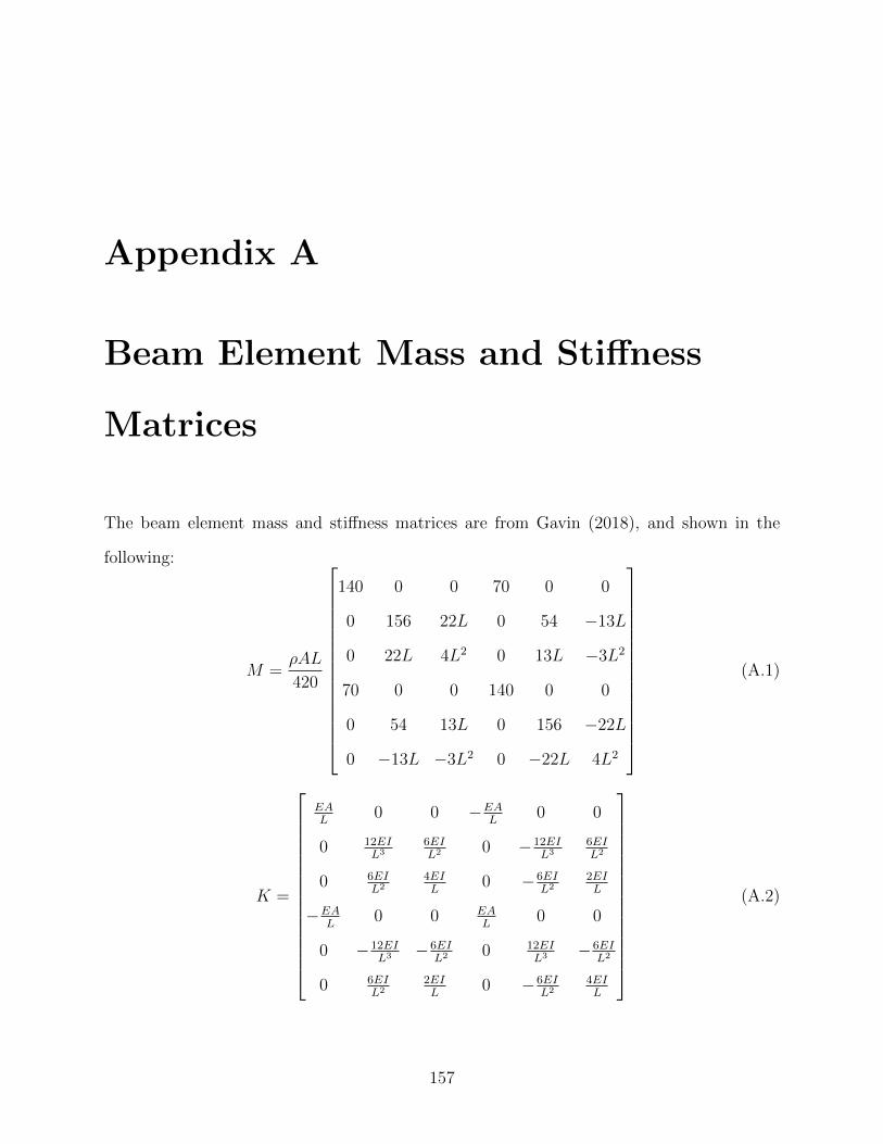
Appendix A

Beam Element Mass and Stiffness

Matrices

The beam element mass and stiffness matrices are from Gavin (2018), and shown in the

following:

M =ρAL

420

140 0 0 70 0 0

0 156 22L 0 54 −13L

0 22L 4L2 0 13L −3L2

70 0 0 140 0 0

0 54 13L 0 156 −22L

0 −13L −3L2 0 −22L 4L2

(A.1)

K =

EAL

0 0 −EAL

0 0

0 12EIL3

6EIL2 0 −12EI

L36EIL2

0 6EIL2

4EIL

0 −6EIL2

2EIL

−EAL

0 0 EAL

0 0

0 −12EIL3 −6EI

L2 0 12EIL3 −6EI

L2

0 6EIL2

2EIL

0 −6EIL2

4EIL

(A.2)

157

Appendix B

Input Constants

158

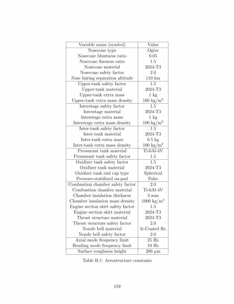
Variable name (symbol) ValueNosecone type Ogive

Nosecone bluntness ratio 0.05Nosecone fineness ratio 1.5

Nosecone material 2024-T3Nosecone safety factor 2.0

Nose fairing separation altitude 110 kmUpper-tank safety factor 1.5

Upper-tank material 2024-T3Upper-tank extra mass 1 kg

Upper-tank extra mass density 100 kg/m3

Interstage safety factor 1.5Interstage material 2024-T3

Interstage extra mass 1 kgInterstage extra mass density 100 kg/m3

Inter-tank safety factor 1.5Inter-tank material 2024-T3

Inter-tank extra mass 0.5 kgInter-tank extra mass density 100 kg/m3

Pressurant tank material Ti-6Al-4VPressurant tank safety factor 1.5Oxidizer tank safety factor 1.5

Oxidizer tank material 2024-T3Oxidizer tank end cap type SphericalPressure-stabilized on-pad False

Combustion chamber safety factor 2.0Combustion chamber material Ti-6Al-4VChamber insulation thickness 3 mm

Chamber insulation mass density 1000 kg/m3

Engine section skirt safety factor 1.5Engine section skirt material 2024-T3

Thrust structure material 2024-T3Thrust structure safety factor 2.0

Nozzle bell material Ir-Coated ReNozzle bell safety factor 2.0

Axial mode frequency limit 25 HzBending mode frequency limit 10 Hz

Surface roughness height 200 µm

Table B.1: Aerostructure constants

159

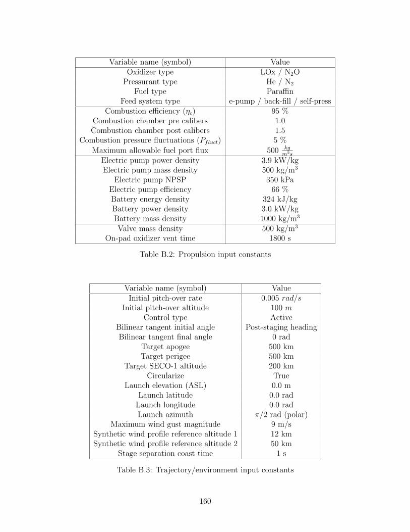
Variable name (symbol) ValueOxidizer type LOx / N2O

Pressurant type He / N2

Fuel type ParaffinFeed system type e-pump / back-fill / self-press

Combustion efficiency (ηc) 95 %Combustion chamber pre calibers 1.0Combustion chamber post calibers 1.5

Combustion pressure fluctuations (Pfluct) 5 %

Maximum allowable fuel port flux 500 kgm2s

Electric pump power density 3.9 kW/kgElectric pump mass density 500 kg/m3

Electric pump NPSP 350 kPaElectric pump efficiency 66 %Battery energy density 324 kJ/kgBattery power density 3.0 kW/kgBattery mass density 1000 kg/m3

Valve mass density 500 kg/m3

On-pad oxidizer vent time 1800 s

Table B.2: Propulsion input constants

Variable name (symbol) ValueInitial pitch-over rate 0.005 rad/s

Initial pitch-over altitude 100 mControl type Active

Bilinear tangent initial angle Post-staging headingBilinear tangent final angle 0 rad

Target apogee 500 kmTarget perigee 500 km

Target SECO-1 altitude 200 kmCircularize True

Launch elevation (ASL) 0.0 mLaunch latitude 0.0 rad

Launch longitude 0.0 radLaunch azimuth π/2 rad (polar)

Maximum wind gust magnitude 9 m/sSynthetic wind profile reference altitude 1 12 kmSynthetic wind profile reference altitude 2 50 km

Stage separation coast time 1 s

Table B.3: Trajectory/environment input constants

160

Appendix C

LEE150 Supplementary Output

C.1 Mission Plots

161

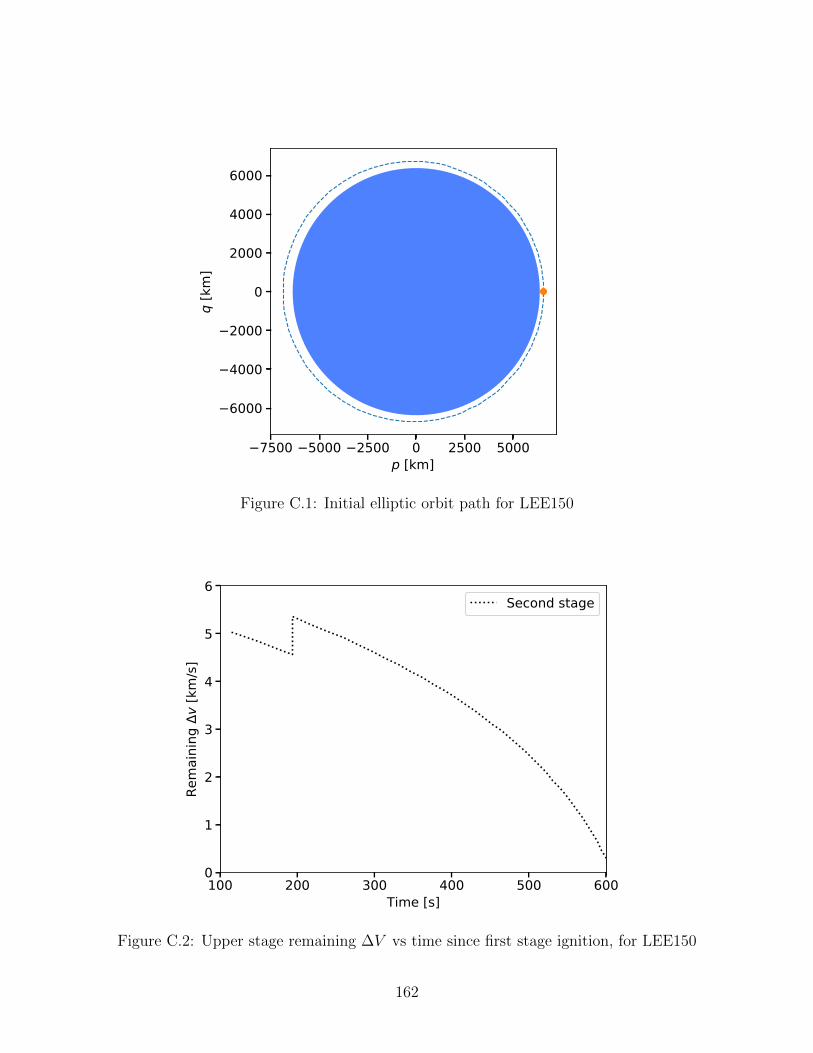
7500 5000 2500 0 2500 5000p [km]

6000

4000

2000

0

2000

4000

6000

q [k

m]

Figure C.1: Initial elliptic orbit path for LEE150

100 200 300 400 500 600Time [s]

0

1

2

3

4

5

6

Rem

aini

ng

v [k

m/s

]

Second stage

Figure C.2: Upper stage remaining ∆V vs time since first stage ignition, for LEE150

162

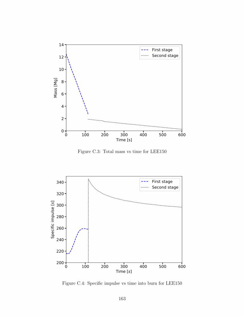
0 100 200 300 400 500 600Time [s]

0

2

4

6

8

10

12

14

Mas

s [M

g]First stageSecond stage

Figure C.3: Total mass vs time for LEE150

0 100 200 300 400 500 600Time [s]

200

220

240

260

280

300

320

340

Spec

ific

impu

lse [s

]

First stageSecond stage

Figure C.4: Specific impulse vs time into burn for LEE150

163

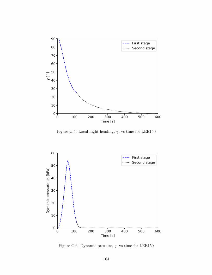
0 100 200 300 400 500 600Time [s]

0

10

20

30

40

50

60

70

80

90

[]

First stageSecond stage

Figure C.5: Local flight heading, γ, vs time for LEE150

0 100 200 300 400 500 600Time [s]

0

10

20

30

40

50

60

Dym

anic

pres

sure

, q, [

kPa]

First stageSecond stage

Figure C.6: Dynamic pressure, q, vs time for LEE150

164

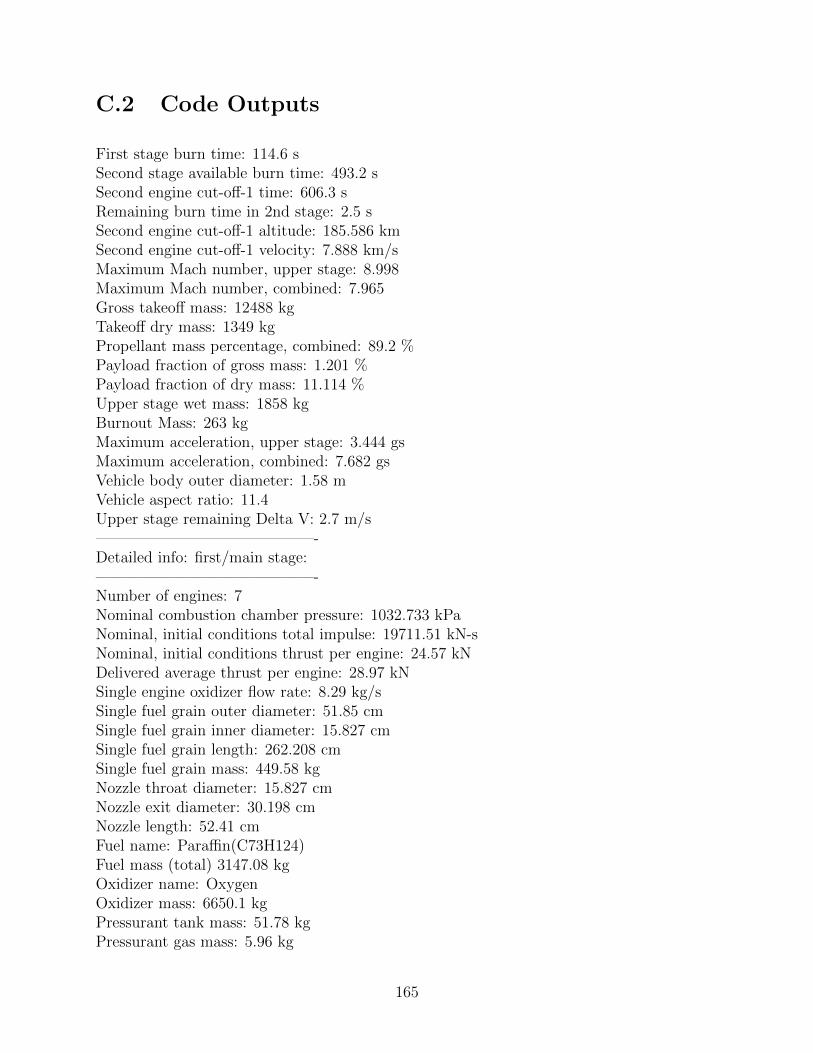
C.2 Code Outputs

First stage burn time: 114.6 sSecond stage available burn time: 493.2 sSecond engine cut-off-1 time: 606.3 sRemaining burn time in 2nd stage: 2.5 sSecond engine cut-off-1 altitude: 185.586 kmSecond engine cut-off-1 velocity: 7.888 km/sMaximum Mach number, upper stage: 8.998Maximum Mach number, combined: 7.965Gross takeoff mass: 12488 kgTakeoff dry mass: 1349 kgPropellant mass percentage, combined: 89.2 %Payload fraction of gross mass: 1.201 %Payload fraction of dry mass: 11.114 %Upper stage wet mass: 1858 kgBurnout Mass: 263 kgMaximum acceleration, upper stage: 3.444 gsMaximum acceleration, combined: 7.682 gsVehicle body outer diameter: 1.58 mVehicle aspect ratio: 11.4Upper stage remaining Delta V: 2.7 m/s——————————————-Detailed info: first/main stage:——————————————-Number of engines: 7Nominal combustion chamber pressure: 1032.733 kPaNominal, initial conditions total impulse: 19711.51 kN-sNominal, initial conditions thrust per engine: 24.57 kNDelivered average thrust per engine: 28.97 kNSingle engine oxidizer flow rate: 8.29 kg/sSingle fuel grain outer diameter: 51.85 cmSingle fuel grain inner diameter: 15.827 cmSingle fuel grain length: 262.208 cmSingle fuel grain mass: 449.58 kgNozzle throat diameter: 15.827 cmNozzle exit diameter: 30.198 cmNozzle length: 52.41 cmFuel name: Paraffin(C73H124)Fuel mass (total) 3147.08 kgOxidizer name: OxygenOxidizer mass: 6650.1 kgPressurant tank mass: 51.78 kgPressurant gas mass: 5.96 kg

165

Electric pump mass (total): 23.99 kgElectric pump battery mass (total): 39.73 kg——————————————-Detailed info: upper stage:——————————————-Number of engines: 1Nominal combustion chamber pressure: 846.903 kPaNominal, initial conditions total impulse: 4548.67 kN-sNominal, initial conditions thrust per engine: 9.22 kNDelivered average thrust per engine: 9.22 kNSingle engine oxidizer flow rate: 2.24 kg/sSingle fuel grain outer diameter: 67.308 cmSingle fuel grain inner diameter: 8.633 cmSingle fuel grain length: 129.294 cmSingle fuel grain mass: 403.57 kgNozzle throat diameter: 8.633 cmNozzle exit diameter: 67.38 cmNozzle length: 155.302 cmFuel name: Paraffin(C73H124)Fuel mass (total) 403.57 kgOxidizer name: OxygenOxidizer mass: 1103.07 kgPressurant tank mass: 8.59 kgPressurant gas mass: 0.99 kgElectric pump mass (total): 0.71 kgElectric pump battery mass (total): 5.06 kg——————————————-Rocket element info for first/main stage:——————————————-NoseconeMaterial: 2024-T6Wall thickness: 1.932 mmSection length: 2.37 m——————————————-Upper-tankMaterial: 2024-T6Wall thickness: 1.769 mmSection length: 0.34 m——————————————-Oxidizer tankMaterial: 2024-T6Wall thickness: 1.244 mmSection length: 0.51 m——————————————-Interstage

166

Material: 2024-T6Wall thickness: 2.64 mmSection length: 4.55 m——————————————-Upper-tankMaterial: 2024-T6Wall thickness: 2.851 mmSection length: 1.42 m——————————————-Oxidizer tankMaterial: 2024-T6Wall thickness: 2.094 mmSection length: 3.55 m——————————————-Inter-tankMaterial: 2024-T6Wall thickness: 3.516 mmSection length: 0.86 m——————————————-EngineMaterial: 2024-T6Wall thickness: 1.455 mmSection length: 4.46 m——————————————-

167