Computing with voting trees

Jennifer Iglesias ∗ Nathaniel Ince † Po-Shen Loh‡

Abstract

The classical paradox of social choice theory asserts that there is no fair way to deterministi-

cally select a winner in an election among more than two candidates; the only definite collective

preferences are between individual pairs of candidates. Combinatorially, one may summarize

this information with a graph-theoretic tournament on n vertices (one per candidate), placing

an edge from u to v if u would beat v in an election between only those two candidates (no ties

are permitted). One well-studied procedure for selecting a winner is to specify a complete binary

tree whose leaves are labeled by the candidates, and evaluate it by running pairwise elections

between the pairs of leaves, sending the winners to successive rounds of pairwise elections which

ultimately terminate with a single winner. This structure is called a voting tree.

Much research has investigated which functions on tournaments are computable in this

way. Fischer, Procaccia, and Samorodnitsky quantitatively studied the computability of the

Copeland rule, which returns a vertex of maximum out-degree in the given tournament. Perhaps

surprisingly, the best previously known voting tree could only guarantee a returned out-degree

of at least log2 n, despite the fact that every tournament has a vertex of degree at least n−12 .

In this paper, we present three constructions, the first of which substantially improves this

guarantee to Θ(√n). The other two demonstrate the richness of the voting tree universe, with

a tree that resists manipulation, and a tree which implements arithmetic modulo three.

1 Introduction

The study of elections is a complex field. When deciding between two candidates, one may consider

several procedures, but the familiar majority vote can actually be shown to have nice mathematical

properties, as described in detail by May in [6]. Unfortunately, these properties are difficult to

extend to a multi-agent election, and far less is understood in that setting. One approach is to

run independent 2-candidate majority elections between pairs of candidates, and select a winner

based upon those results. Combinatorially, running all such elections would produce a tournament

(an oriented complete graph, in which every pair of vertices spans exactly one directed edge)

summarizing all pairwise preferences.

∗Department of Mathematical Sciences, Carnegie Mellon University, Pittsburgh, PA 15213, e-mail: jigle-

sia@andrew.cmu.edu.†Department of Mathematical Sciences, Carnegie Mellon University, Pittsburgh, PA 15213, e-mail:

nince@andrew.cmu.edu.‡Department of Mathematical Sciences, Carnegie Mellon University, Pittsburgh, PA 15213. E-mail: ploh@cmu.edu.

Research supported by NSF grant DMS-1201380, an NSA Young Investigators Grant and a USA-Israel BSF Grant.

1

Yet even though such a tournament contains much information about the candidates, selecting

a winner given such a tournament, known in the social sciences as a tournament solution, is a

difficult question. Indeed, McGarvey [7] showed that even with a number of voters only polynomial

in n (the number of agents), every possible tournament is already achievable in this way. So, there

may be many lists of preferences among multiple agents that fit the same description. One natural

method is to select a candidate that beats as many other candidates as possible in the pairwise

majority elections. This is known as the Copeland solution, and is equivalent to identifying a

vertex of maximum out-degree in the preference tournament. Such a vertex may not be unique,

so it is desirable to develop a procedure which selects a vertex with similar properties, while being

completely deterministic. One natural solution is to construct a voting tree, and this paper analyzes

the combinatorial aspects of such structures, inspired by recent work of Fischer, Procaccia, and

Samorodnitsky [4].

We first coordinate our terminology with that typically used in the social science literature. Let

Tn denote the set of all tournaments on the vertex set [n]. An agenda is a mapping from Tn to [n].

A match Mi,j is a particular agenda of the form

Mi,j(T ) =

i if i = j or

−→ij ∈ T ;

j otherwise.

We will refer to Mi,j as the match between i and j. Using this as the basic building block,

we may now interpret certain labeled binary trees as agendas. Indeed, let S be a (not necessarily

complete) binary tree, in which each node has either 0 or 2 children, where each leaf is labeled

with an integer in [n]. We permit multiple leaves to receive the same label. The corresponding

agenda A is computed as follows. Given a tournament T on [n], we recursively label each node of

the tree S by the result of the match between its children’s labels. The ultimate label at the root

is the output of this agenda, and such agendas are called voting trees. For instance, Mi,j may be

represented by a three node binary tree, as shown below.

i j

Figure 1: The Mi,j voting tree.

Voting trees were first introduced by Farquharson in [3] and further investigated by various

researchers in [8], [10], [11], [12], and [13]. Fischer, Procaccia, and Samorodnitsky focused on

the problem of quantitatively approximating the Copeland solution with voting trees. A voting

system which is implementable by a voting tree, implies that the system is also implementable via

backwards induction, as shown in [2]. Both [1] and [5] provide social choice functions which are

implementable via backwards induction.

Let the performance guarantee of a given voting tree Θ be the minimum out-degree which it

2

ever produces on any input, i.e.,

minT∈Tnout-degree of Θ(T ) .

When the number of agents n is a power of two, it is relatively easy to construct a voting

tree with performance guarantee log2 n: take a complete binary tree with n leaves, and label the

leaves with an arbitrary permutation of [n]. Then, given any tournament as input, the ultimate

winner must win exactly log2 n matches on the way to the root, and since all leaves are distinctly

labeled, the winner must have met a different opponent at each of those matches. Therefore, the

winner must always have out-degree at least log2 n. On the other hand, for this voting tree, an

adversary can easily construct a suitable tournament to provide as input such that the winner only

has out-degree exactly log2 n. In contrast, it is well-known that every n-vertex tournament has a

vertex of out-degree at least (n− 1)/2, so this performance guarantee appears to be quite weak.

Perhaps surprisingly, prior to our work, this was the best known voting tree according to this

metric, despite non-trivial effort: in [4], the problem of improving this lower bound was even

suspected to currently be “out of reach.” Fischer, Procaccia, and Samorodnitsky also proved the

strongest negative result, showing that no tree can guarantee a winner with out-degree at least

3/4 of the maximum out-degree in the input tournament; in particular, quantifiably strengthening

an earlier result of Moulin [9] which showed that no voting tree can always identify the Copeland

solution. Srivastava and Trick [13] showed that Moulin’s result is also a minimal example. However,

these lower and upper bounds are extremely far apart, and even the case n = 6 is still not settled.

This article proves a number of positive results which demonstrate the rather rich computational

power of voting trees. We first exhibit a construction which substantially improves the logarithmic

lower bound of the trivial construction above.

Theorem 1.1. There exist voting trees Ωn with performance guarantee at least (√

2 + o(1))√n.

We then show two constructions which we discovered while investigating this problem. We feel

that they may be of independent interest, to different communities. The first is relevant to social

choice theory, and achieves a rather counterintuitive result. As motivation, observe that any upper

bound for our problem consists of a procedure that takes a voting tree as input, and produces a

suitable tournament as output, such that when tree is applied to the tournament, the resulting

winner has low out-degree. The most natural candidate tournaments have the following form.

Definition 1.2. A perfect manipulator tournament is an n-vertex tournament with vertex set

α∪B∪C, where B and C are nonempty, the single element α (the “manipulator”) defeats every

member of B, every member of B defeats every member of C, and every member of C defeats α.

One might suspect that given any voting tree, if one wants to design a tournament for which a

particular vertex α ∈ [n] is the winner, this should be accomplished by having all vertices that α

defeats able to beat all vertices that win against α, i.e., by constructing a suitable perfect manip-

ulator tournament. The task of improving the upper bound would then be reduced to specifying

and controlling the size of the set B of vertices defeated by the manipulator α. Surprisingly, this

intuition is completely incorrect.

3

Theorem 1.3. For every integer n ≥ 4 which is a power of two, there is a voting tree Ψ such that

for every α ∈ [n] and every perfect manipulator tournament T with α as the manipulator, α does

not win when Ψ is applied to T .

Note that the result holds regardless of how large B is, and in particular, even if C, the set of

agents who defeat α, has size as small as 1. The result obviously cannot hold for all n, because,

for example, for n = 3, one can construct a suitable perfect manipulator tournament for any tree

Θ by letting T be the unlabeled directed 3-cycle, and feeding it into Θ; whichever vertex wins is

labeled as the manipulator α, and B and C are assigned cyclically. Ad-hoc constructions exist for

several other values of n, but these are not easily generalizable.

Our final construction demonstrates that voting trees can be harnessed for computation. The

first voting tree we discovered that beat the logarithmic lower bound was built using “arithmetic

gates” which operated on the most fundamental case n = 3. This is a voting tree analogue of the

classical arithmetic circuits built from AND and OR logical gates.

Theorem 1.4. There exist voting trees Σ and Π, with leaves labeled by 0, 1, 2, X, Y , with the

following properties. Let T be an arbitrary non-transitive tournament on the vertex set F3 =

0, 1, 2, i.e., one of the two cyclic orderings of the vertex set. Let x and y be arbitrary elements

of F3. Then, if in Σ and Π, all occurrences of X and Y are replaced by x and y, and both trees are

evaluated on T , their corresponding outputs are precisely the elements in F3 corresponding to x+ y

and xy, respectively.

These trees Σ and Π can be interpreted as addition and multiplication gates in the context of

voting trees, where the X and Y represent the two inputs to each gate. These gates can then be

chained together as robust building blocks which independently perform consistently across input

tournaments. The requirement of non-transitivity is essential, because if a transitive tournament

is input, no non-trivial voting tree can avoid having the dominant vertex win.

2 Lower bound

We now move to describe the constructions. We start by creating voting trees Ωn with performance

guarantees of (√

2 + o(1))√n, where n is the number of agents. The following tree serves as our

fundamental building block.

Definition 2.1. Let i be a label between 1 and n inclusive, and let S ⊂ [n] \ i be a set of other

labels. Construct the complete binary tree with exactly |S| pairs of leaves, and for each label s ∈ S,

place the labels i and s on a distinct pair of leaves, as illustrated in Figure 2. We call the resulting

voting tree Λi:S.

The consequences of placing candidate i in competition with every candidate in S turn out to

be quite convenient.

Lemma 2.2. When Λi:S is evaluated on a tournament T , the result is either i, if i defeats every

element of S according to T , or the result is some vertex s ∈ S with the property that s defeats i in

T .

4

3 33 3 3

2 46 8 10

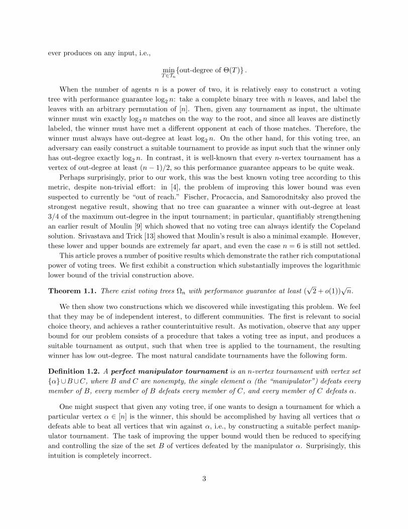
Figure 2: The Λ3:S voting tree for S = 2, 4, 6, 8, 10.

Proof. The leaves of this tree consist of independent pairwise matches between i and every candidate

in S. We start by evaluating the pairwise matches at the leaves, writing the winners of those |S|matches on their parents, and deleting the original leaves. Each of those winners will either be i

(if i won the match), or a candidate of S who defeats i. In particular, at this point, if i defeats

every candidate in S, then i is the only label that remains, and the winner is clearly i, as claimed.

Otherwise, all leaves of the tree are now labeled with only two types of candidates: i itself, and a

nonempty sub-collection R ⊂ S of candidates from S who defeat i.

We now continue to evaluate the tree. Whenever two elements of R are matched against each

other, one wins, and one element of R moves on as the winner. However, whenever an element of R

is matched against i, the element of R wins, and moves on as the winner. Thus, as the evaluation

continues, there is always at least one element of R. This holds all the way up to the root layer,

and so we conclude that the winner of Λi:S is an element of R, i.e., a candidate who defeats i, as

claimed.

We now construct our voting trees Ωn recursively. The following lemma steadily improves the

performance guarantee as the number of candidates increases.

Lemma 2.3. Let Ωn be a voting tree for n agents with performance guarantee k. Then there is a

voting tree Ωn+k+1 for n+ k + 1 agents with performance guarantee at least k + 1.

Proof. To simplify notation, let the n+k+1 candidates be indexed 0, 1, . . . , n+k. Let N =(n+kn

),

and consider the tree Λ0:[N ] from Lemma 2.2, where [N ] = 1, 2, . . . , N. For each i ∈ [N ],

arbitrarily select a distinct subset S ⊂ [n + k] of size n, and remove the leaf labeled i from our

original Λ0:[N ]. In its place, insert the tree ΩS , defined as the voting tree Ωn for n candidates with

performance guarantee k, but labeled with the n elements of S instead of the n elements 1, . . . , n.We claim that the resulting tree guarantees that the winner has out-degree at least k + 1.

Indeed, suppose that it has been fed a tournament on 0, . . . , n + k as input. First, evaluate all(n+kn

)of the ΩS subtrees, and write their winning candidates at their roots. The key observation is

that at least k + 1 distinct candidates emerge from these subtrees. Indeed, let W be the collection

of all such intermediate winners. If |W | ≤ k, then there would be some n-set S′ ⊂ [n + k] which

was disjoint from W . The winner of ΩS′ would then be outside W , contradiction.

At this point, we have the structure of Λ0:[N ], except that the set W appears as the non-0-

labeled leaves. By Lemma 2.2, either candidate 0 wins, in which case it defeats every candidate in

W (producing out-degree at least k + 1), or some candidate w ∈W wins, defeating candidate 0 as

well. Since the out-degree guarantee for w was already k from its ΩS , in which candidate 0 did not

appear, we conclude that w has out-degree at least k + 1, completing the other scenario.

5

Our main asymptotic lower bound now follows by induction.

Proof of Theorem 1.1. For n = 2, we take a single match between candidates 1 and 2, and it is

clear that this guarantees that the winner has out-degree at least 1. Repeated application of the

previous lemma then produces voting trees for k(k+1)2 + 1 candidates which guarantee out-degree

at least k.

3 Perfect manipulator tournaments

We now proceed to our second result. For this construction, let us fix n = 2d as a power of two.

We begin by introducing compact notation that we will use to describe various voting trees in this

section, all of which will be complete binary trees with full bottom layers. We represent such a tree

by listing its leaves from left to right as an m-tuple (x1, x2, . . . , xm) of integers in [n], where m is

a power of two. For example, the n-tuple (1, 2, . . . , n) corresponds to the voting tree mentioned in

the introduction, which achieved the previous best performance guarantee of log2 n.

Using the above notation, we now describe our first gadget, which we will use as a building

block in our construction. We will show that it has the property that when it is applied to any

perfect manipulator tournament α∪B ∪C, then the winner is never in C. It is perhaps intuitive

that such a voting tree might exist, because candidates in C only have a single candidate α who

they are capable of defeating, and therefore have a disadvantage.

Definition 3.1. Define the permutation φ of [n] as:

φ(i) =

(i+ 1)/2 if i is odd, and

n/2 + i/2 if i is even.

Let Φ be the voting tree corresponding to the 2n-tuple (1, . . . , n, φ(1), . . . , φ(n)).

1 2 3 4 5 6 7 8 1 5 2 6 3 7 4 8

Figure 3: The voting tree Φ for n = 8.

This tree is illustrated in Figure 3. The action of the permutation is so that the right half of

the tree is a perfect shuffle of the left half of the tree. The utility of this structure will become clear

in the proof of the following lemma.

Lemma 3.2. Whenever Φ is applied to any perfect manipulator tournament, the winner is not in

C.

6

Proof. Suppose for contradiction that Φ has been applied to such a tournament, and that the

winner is in C. The final match of Φ was between the winners of its left and right subtrees, which

we will refer to as ΦL and ΦR. Note that by the assumption that a member of C won, the final

match must have been between α and an element of C, or between two elements of C, so neither

subtree’s winner can be in B.

Assume that the winner of ΦL is in C. Note that ΦL corresponds to the n-tuple (1, . . . , n), as

defined at the beginning of this section. So ΦL’s leaves contain every element of the tournament

exactly once, and the label α appears in either ΦL’s left or right subtree as a leaf. Without loss of

generality, suppose that α appears in the left subtree of ΦL. Any match between an element of B

and something other than α will be won by an element of B. So the right subtree of ΦL will be

won by an element of B if any elements of B appear on its leaves, then making it impossible for ΦL

to be won by an element of C. Thus, the right subtree of ΦL’s must have all of its leaves labeled

from C.

In ΦR, each label 1, . . . , n2 is initially matched against a label of n2 + 1, . . . , n, due to the action

of the shuffle φ. These labels appear on the leaves of the left and right subtrees of ΦL, respectively.

So in ΦR, α is matched with an element of C, and eliminated in the first round. Since at B is

nonempty, the elements of B will continue to dominate every match of ΦR, unchallenged by α, and

an element of B will win ΦR. It then will beat the element of C that won ΦL, making the winner

of Φ an element of B, contradicting our assumptions.

The other possibility is that ΦR is won by an element of C. The same argument we used on

ΦL shows that either the left or the right subtree of ΦR has leaves entirely contained in C. Let us

suppose that it is the right subtree of ΦR, as the other case is similar. This right subtree contains

the nodes φ(n2 + 1), . . . , φ(n) = n4 + 1, . . . , n2 ∪ 3n4 + 1, n. These are the nodes of the right

subtree of the left subtree of ΦL and the right subtree of the right subtree of ΦL. So it’s clear that

those trees must have winners in C. Therefore α cannot be the winner of either the left or right

subtree of ΦL.

However, α must be initially matched with an element of b ∈ B in ΦR, because otherwise it will

be eliminated in the first round, and B will win ΦR unchallenged, contradicting our assumption that

ΦR is won by C. Since φ alternately maps indices of the left and right subtrees of ΦL into matched

pairs, the two subtrees of ΦL have the property that one contains α, and the other contains b and

not α. As before, the latter subtree will be won by B, and the previous paragraph’s conclusion

implies that the other subtree of ΦL is not won by α. Therefore, ΦL is won by B, which then

defeats the element of C which we assumed as the winner of ΦR, contradicting the fact that Φ was

won by C.

Our next gadget enables us to force α to lose by transferring the status of the “perfect manip-

ulator” to another node of T . For each i ∈ [n], define Λi to be the voting tree Λi:S from Definition

2.1, with S = [n]\i. To unify notation, let A = α in the perfect manipulator tournament. The

same argument as used in Lemma 2.2 shows that the winners of this tree “rotate” the sets A, B,

and C.

Lemma 3.3. When Λi is evaluated on a perfect manipulator tournament T , the winner is in C if

i ∈ A, in A if i ∈ B, and in B if i ∈ C.

7

Proof. Without loss of generality, suppose that i ∈ A. After all of the initial leaf matches are

evaluated, all intermediate winners are either from A or C, because all candidates from C were

immediately eliminated by i. Importantly, since all three classes A, B, and C are nonempty in

perfect manipulator tournaments, at least one element of C survives. Now all remaining candidates

are from either A or C, and so just as in the proof of Lemma 2.2, C is unchallenged, and an element

of C emerges as the winner.

Next, we compose Λi with itself to perform a “double rotation” on perfect manipulator tourna-

ments.

Definition 3.4. For any i ∈ [n], start with the voting tree Λi. At each leaf, note the label (suppose

it was j), erase the label, and then insert a copy of Λj with its root at that leaf. Call the result Λ2i .

Corollary 3.5. When Λ2i is evaluated on a perfect manipulator tournament T , the winner Λ2

i (T )

is in B if i ∈ A, in C if i ∈ B, and in A if i ∈ C.

Proof. Without loss of generality, suppose that i ∈ A. By Lemma 3.3, the winner of Λi is in C,

and elements of both B and A are represented amongst the winners of the other Λj . Therefore,

the previous lemma’s argument implies that the winner of Λ2i is from the set which defeats C, i.e.,

B.

We are now ready to describe our main construction for this section. Start with the voting tree

Λ2j and replace each leaf labeled j with a copy of the voting tree Φ from Definition 3.1 and call the

resulting tree Ψ.

Proof of Theorem 1.3. Let T be the perfect manipulator tournament given as input. With respect

to T , when Φ is evaluated we will be given a vertex which is not in C. Now when something which

is not C is feed as input into Λ2i then we get something which is not in A by Corollary 3.5. So, the

output of the whole tree Ψ will not be α as desired.

4 Arithmetic circuits

In this section, we construct more complex chains of voting trees for n = 3 which can perform

arithmetic modulo three. An essential caveat is that such computation is clearly impossible when

the input tournament is transitively oriented, and so we design our circuits to succeed no matter

which non-transitive tournament is input. The two such tournaments are shown in Figure 4.

We will now create trees of increasing complexity by developing robust “gates” and putting

them together. However, this time, because our aim is to send outputs of gates as inputs into other

gates, we will design voting trees whose leaves are labeled with both tournament vertices (0, 1, 2)

and variables X, Y , etc. Our basic building block, which we call a yield gate, is again along the

lines of Definition 2.1, and is illustrated in Figure 5.

The same argument as used in the proof of Lemma 3.3 produces the following conclusion.

Corollary 4.1. For any non-transitive tournament T and any vertex x ∈ T , if all labels X are

replaced with x in the yield gate, and the tree is evaluated with respect to T , then the winner is the

unique vertex which beats x.

8

0

12

0

12

Figure 4: There are two non-transitive tournaments on three vertices. We call the tournament on the left the

clockwise tournament, and the tournament on the right the counter-clockwise tournament.

X 0 X 1

X 2

Figure 5: A yield gate, a tree which outputs a candidate which beats the input X.

4.1 Addition

Next, we combine yield gates to create a negative sum gate, which takes X and Y as inputs,

and outputs −X − Y (modulo 3) with respect to any non-transitive tournament. A simple match

between two yield gates, shown in Figure 6, almost achieves this behavior.

X 0 X 1 Y 0 Y 1

X 2 Y 2

Figure 6: A simple combination of two yield gates.

Let us analyze the behavior of this tree with respect to the various tournaments and inputs

X and Y . If X = Y , then both halves of the tree return the same output, which is X − 1 for

the clockwise tournament, and X + 1 for the counter-clockwise tournament. Now consider the

case where X 6= Y , and let Z be the third vertex (so Z = 0, 1, 2 \ X,Y ). In the clockwise

tournament, the two halves of the tree would return X − 1 and Y − 1. If X = Y − 1 then X − 1

would beat Y − 1, producing X − 1 as the winner. Here, X − 1 = Z because X − 1 is neither

X nor Y . On the other hand, if Y = X − 1 then we would have the result be Y − 1 which is

again Z. Doing the same calculations for the counter-clockwise tournament, we get that X + 1

wins if X = Y + 1, and Y + 1 wins if Y = X + 1. In summary, whenever X 6= Y , regardless of the

9

tournament’s orientation, the output is Z, which equals −X −Y because X,Y, Z = 0, 1, 2 and

0 + 1 + 2 = 0. So the gate shown in Figure 6 gives us the desired outcome of −X−Y when X 6= Y .

We will now stack several gates of this type together to create our desired gate, as illustrated in

Figure 7.

X

Y

X

Y

X

Y

Figure 7: This circuit computes −X − Y . Each triangular gate in this arrangement is a copy of the gate shown in

Figure 6. The two inputs on the left of each gate correspond to X and Y , and the output on the right is the output

of the tree. When the output of a structure is plugged into (say) the X-input of another gate, all copies of X in the

latter gate are replaced with identical copies of the structure.

Lemma 4.2. The gate in Figure 7 computes −X − Y .

Proof. First we consider the case X 6= Y , and let Z = 0, 1, 2 \ X,Y . So, the output of both

leftmost trees is −X − Y = Z. Now Z 6= X and Z 6= Y so the next layer of trees output Y and X

respectively. The last gate receives Y and X as input, so outputs −X − Y as desired.

Now we consider the case X = Y , starting with the clockwise tournament. By the discussion

above, both leftmost trees output X − 1. Now the second layer of trees receive X and X − 1 as

input, and therefore both give X + 1 as output. The last tree now receives X + 1 for both inputs,

and so gives (X + 1)− 1 as output. This is our desired outcome as −X −X = X (modulo 3). In

the final case, where X = Y and the tournament is counter-clockwise, similar calculations yield

that the last layer outputs (X − 1) + 1 = X = −X −X as desired.

Observe that if we send the constant 0 as the input for Y in the −X − Y gate, we produce a

unary negation gate. If we then feed the output of the negative sum tree through this negation

tree, then the output becomes the ordinary sum X + Y , which was the objective of this section.

Corollary 4.3. There is a gate which takes inputs X and Y , and outputs their sum X + Y (in

F3), when evaluated with respect to any non-transitive tournament on three vertices.

The gates constructed thus far will be used repeatedly in later sections, and Figure 8 shows

how they will be compactly represented in the remainder of this paper.

- +Figure 8: These symbols will represent (from left to right) the negation gate, addition gate, and yield gate. Inputs

enter the left side of each gate and outputs exit via the right side of the gate.

10

4.2 Squaring

Having created our addition gate, we move toward multiplication. To this end, in this section we

develop a unary gate which computes the function X 7→ X2, regardless of which non-transitive

3-vertex tournament is used. Observe that the squaring function sends 0 to 0, and sends both 1

and 2 to the same value 1. We start by creating a gate (shown in Figure 9) with similar properties.

X

12

X

21

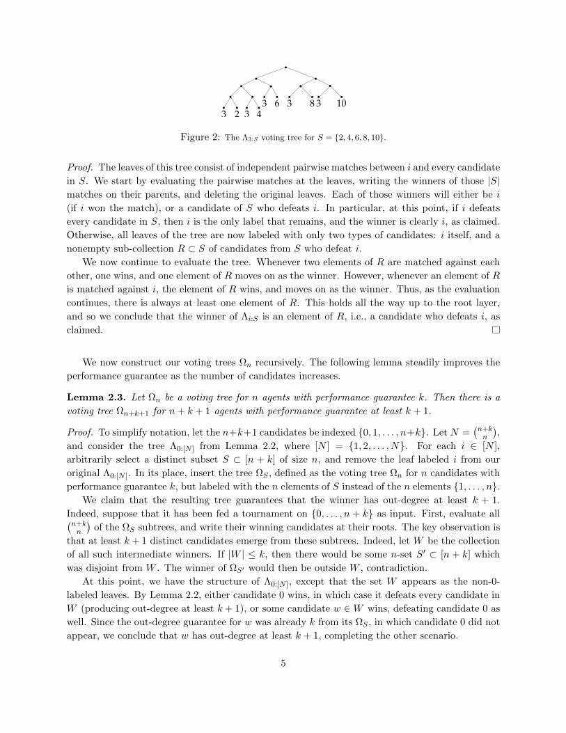
Figure 9: The first half of the squaring gate. The final merging on the right side represents an ordinary voting tree

comparison between the outputs of the top and bottom chain of gates.

Lemma 4.4. The gate in Figure 9 sends 0 7→ 0, 1 7→ 2, and 2 7→ 2 on the clockwise tournament,

and 0 7→ 2, 1 7→ 1, and 2 7→ 1 on the counter-clockwise tournament.

Proof. Consider the clockwise tournament. On the top left of the gate, if X = 0 then 0 beats 1

and then 2 beats 0. Otherwise, the top left is simply the winner between 1 and 2, which in this

case is 1. Feeding this through the yield gate twice we get the top produces 0 when 0 is input,

and 2 when either 1 or 2 are input. On the bottom left of the tree, if X = 0 then 2 beats 0 and

then 1 beats 2. Otherwise, the bottom left is again the winner between 1 and 2 which is again 1.

So, for the clockwise tournament, the bottom always feeds 1 through a yield gate and produces 0,

regardless of the input X. Matching the outputs of the top and the bottom, and evaluating with

respect to the clockwise tournament, we find that the gate in Figure 8 outputs 0 if X = 0 and

outputs 2 otherwise, as claimed.

It remains to consider the counter-clockwise tournament. On the bottom left of the tree, if

X = 0 then 0 beats 2 and then 1 beats 0. Otherwise, the bottom left is simply the winner between

1 and 2, which is 2. Feeding this through the yield gate, we find that the bottom is 2 when 0 is

input, and 0 when either 1 or 2 are input. On the top left of the tree, if X = 0 then 1 beats 0

and then 2 beats 1. Otherwise, the top left is again the winner between 1 and 2 which is again 2.

So, for the counter-clockwise tournament, the top always feeds 2 through a yield gate twice and

produces 1, regardless of the input X. Combining the top and the bottom we conclude that the

gate outputs 2 if X = 0 and outputs 1 otherwise.

At this point we are relatively close to getting the desired outcome, as for each non-transitive

tournament, the inputs 1 and 2 produce one result, and the input 0 produces a different one. We

complete our squaring gate by sending this output into the gate shown in Figure 10.

Lemma 4.5. The composition of the gates in Figures 9 and 10 computes the function X 7→ X2.

11

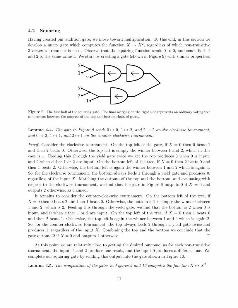
- +Y

1

Figure 10: The second half of the squaring gate. Here, Y is used to represent the input to this half, so there is no

confusion with the input X to the first half (from Figure 9).

Proof. Let Y be the output of the gate in Figure 9 when X is input. In the case of the clockwise

tournament, Y = 0 if X = 0 and Y = 2 otherwise. Feeding this through the two yield gates, we get

1 when X = 0 and 0 otherwise. In the case of the counter-clockwise tournament, Y = 2 if X = 0

and Y = 1 otherwise. When this passes through two yield gates, then we again get 1 when X = 0

and 0 otherwise. So, regardless of the tournament used, the result after the two yield gates is 1

when X = 0, and 0 otherwise. We wish to have 0 when X = 0 and 1 otherwise. This is achieved

by subtracting our current result from 1, which is realized by the negation and addition gates in

the right half of Figure 10.

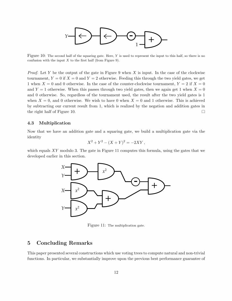
4.3 Multiplication

Now that we have an addition gate and a squaring gate, we build a multiplication gate via the

identity

X2 + Y 2 − (X + Y )2 = −2XY ,

which equals XY modulo 3. The gate in Figure 11 computes this formula, using the gates that we

developed earlier in this section.

+ x2

++-

X

Y

X

Y

x2

x2

Figure 11: The multiplication gate.

5 Concluding Remarks

This paper presented several constructions which use voting trees to compute natural and non-trivial

functions. In particular, we substantially improve upon the previous best performance guarantee of

12

log2 n, constructing trees which achieve order√n. We presented our arithmetic gates in our final

section because they were initially developed for lower bound constructions for the performance

guarantee, and produced our first construction which improved the lower bound. We also feel that

they may be of independent interest, as they demonstrate that the computational power of voting

trees is sufficiently rich to perform standard ternary arithmetic.

References

[1] P. J. Coughlan and M. Le Breton, A social choice function implementable via backward induc-

tion with values in the ultimate uncovered set, Rev Econ Des 4 (1999), 153–160.

[2] B. Dutta and A. Sen, Implementing generalized Condorcet social choice functions via backward

induction, Soc Choice Welfare 10 (1993), 149–160.

[3] R. Farquharson, Theory of Voting, Yale University Press, New Haven, 1969.

[4] F. Fischer., A. D. Procaccia, and A. Samorodnitsky, A new perspective on implementation by

voting trees, Random Structures and Algorithms 39 (2011), 59–82.

[5] M. Herrero and S. Srivastava, Implementation via backward induction, J Econ Theory 56

(1992), 70–88.

[6] K. May, A set of independent, necessary and sufficient conditions for simple majority decisions,

Econometrica 20 (1952), 680–684.

[7] D. C. McGarvey, A theorem on the construction of voting paradoxes, Econometrica 21 (1953),

608–610.

[8] R. D. McKelvey, R. G. Niemi, A multistage game representation of sophisticated voting for

binary procedures, J. Econ. Theory. 18 (1978), 1–22.

[9] H. Moulin, Choosing from a tournament, Soc Choice Welfare 3 (1986) 271–291.

[10] N. Miller, A new solution set for tournaments and majority voting: further graph theoretical

approaches to the theory of voting. Am. J. Pol. Sci. 24 (1980), 68-96.

[11] N. Miller, Graph theoretical approaches to the theory of voting, Am. J. Pol. Sci. 21 (1977),

769-803.

[12] J. Moon, Topics on tournaments, Holt, Rinehart and Winston, New York, 1968.

[13] S. Srivastava and M. A. Trick, Sophisticated voting rules: The case of two tournaments, Soc

Choice Welfare 13 (1996), 275–289.

13