COMPUTING THE NUMBER OF TYPES OF INFINITELENGTH

WILL BONEY

Abstract. We show that the number of types of sequences of tuples of a fixedlength can be calculated from the number of 1-types and the length of thesequences. Specifically, if κ ≤ λ, then

sup‖M‖=λ

|Sκ(M)| =

(sup‖M‖=λ

|S1(M)|

)κWe show that this holds for any abstract elementary class with λ amalgamation.Basic examples show that no such calculation is possible for nonalgebraic types.However, we introduce a generalization of nonalgebraic types for which the sameupper bound holds.

Contents

1. Introduction 12. Preliminaries 23. Results on Sα(M) 84. Strongly Separative Types 165. Saturation 226. Further Work 24References 25

1. Introduction

A well-known result in stability theory is that stability for 1-types implies stabil-ity for n-types for all n < ω; see Shelah [Sh:c] Corollary I.§2.2 or Pillay [Pil83].0.9.In this paper, we generalize this result to types of infinite length.

Theorem 1.1. Given a complete theory T , if the supremum of the number of 1-types over models of size λ ≥ |T | is µ, then for any (possibly finite) cardinal κ ≤ λ,the supremum of the number of κ-types over models of size λ is exactly µκ.

We do this by using the semantic, rather than syntactic, properties of types.This allows our arguments to work in many nonelementary classes. Thus, we work

Date: May 8, 2014.1

2 WILL BONEY

in the framework of Abstract Elementary Classes (AECs), which was introducedby Shelah in [Sh88]. As we discuss in Section 2, AECs and Galois types includeelementary classes and syntactic types and various nonelementary classes, such asthose axiomatized in Lλ+,ω(Q). We use our results to answer a question of Shelahfrom [Sh:c].

While the number of types of sequences of infinite lengths has not been cal-culated before, these types have already seen extensive use under the name tp∗in [Sh:c] and TP∗ in [Sh:h].V.D.§3. While [Sh:c] uses them most extensively, it isthe use in [Sh:h].V.D.§3 as types of models that might be most useful. This meansthat stability in λ can control the number of extensions of a model of size λ; seeSection 3.

After seeing preliminary versions of this work, Rami Grossberg asked if theabove theorem could be proved for nonalgebraic types. The examples in Propo-sition 4.1 show that such a theorem is not possible, even in natural elementaryclasses. However, we introduce a generalization of nonalgebraic types of tuplescalled strongly separative types for which we can prove the same upper bound. InAECs with disjoint amalgamation, such as elementary classes, nonalgebraic andstrongly separative types coincide for types of length 1. For longer types, we re-quire that realizations are, in a sense, nonalgebraic over each other. For instance,in ACF0, the type of (e, π) can be considered “more nonalgebraic” over the set ofalgebraic numbers than the type of (e, 2e). This is made precise in Definition 4.2.

Finally, in Section 5, we investigate the saturation of types of various lengths.The “saturation = model homogeneity” lemma (recall Lemma 2.10) shows thatsaturation is equivalent for all lengths. We also use bounds on the number of typesand various structural properties to construct saturated models.

This paper was written while working on a Ph.D. under the direction of RamiGrossberg at Carnegie Mellon University and I would like to thank Professor Gross-berg for his guidance and assistance in my research in general and relating to thiswork specifically. A preliminary version of this paper was presented in the CMUModel Theory Seminar and I’d like to thank the participants for helping to im-prove the presentation of the material, especially Alexei Kolesnikov. He pointedout a gap in the proof of Theorem 3.2 and vastly improved the presentation ofTheorem 3.5, among many other improvements. I would also like to thank mywife Emily Boney for her support.

2. Preliminaries

We use the framework of abstract elementary classess to prove our results. Thus,we offer the following primer on abstract elementary classes and Galois types.

The definition for an abstract elementary class (AEC) was first given by Shelahin [Sh88]. The definitions and concepts in the section are all part of the litera-ture; in particular, see Baldwin [Bal09], Shelah [Sh:h], Grossberg [Gro02], or theforthcoming Grossberg [Gro1X] for more information.

COMPUTING THE NUMBER OF TYPES OF INFINITE LENGTH 3

Definition 2.1. We say that (K,≺K) is an Abstract Elementary Class iff

(1) There is some language L = L(K) so that every element of K is an L(K)-structure;

(2) ≺K is a partial order on K;(3) for every M,N ∈ K, if M ≺K N , then M ⊆L N ;(4) (K,≺K) respects L(K) isomorphisms, if f : N → N ′ is an L(K) isomor-

phism and N ∈ K, then N ′ ∈ K and if we also have M ∈ K with M ≺K N ,then f(M) ∈ K and f(M) ≺K N ′;

(5) (Coherence) if M0,M1,M2 ∈ K with M0 ≺K M2, M1 ≺K M2, and M0 ⊆M1, then M0 ≺M1;

(6) (Tarski-Vaught axioms) suppose 〈Mi ∈ K : i < α〉 is a ≺K-increasingcontinuous chain, then(a) ∪i<αMi ∈ K and, for all i < α, we have Mi ≺K ∪i<αMi; and(b) if there is some N ∈ K so that, for all i < α, we have Mi ≺K N , then

we also have ∪i<αMi ≺K N ; and(7) (Lowenheim-Skolem number) LS(K) is the minimal infinite cardinal λ ≥|L(K)| such that for any M ∈ K and A ⊂ |M |, there is some N ≺K Msuch that A ⊂ |N | and ‖N || ≤ |A|+ λ.

Remark 2.2. We drop the subscript on ≺K when it is clear from context andwe abuse notation by calling K an AEC when we mean that (K,≺K) is an AEC.We follow the convention of Shelah and use ‖M‖ to denote the cardinality of theuniverse of M . In this paper, K is always an AEC that has no models of sizesmaller than the Lowenheim-Skolem number.

The most basic example of an AEC is any elementary class with the elemen-tary substructure relation. In particular, they are structural properties that canbe proved without mention of the compactness theorem. This means that classesof models axiomatized in many other logics, such as those with infinite conjunc-tion/disjunction or with additional quantifiers, are also AECs with the appropri-ate substructure relation. [Bal09].4 and [Bal07] give more details and [BET07]discusses AECs consisting of modules.

We will briefly summarize some of the basic notations, definitions, and resultsfor AECs.

Definition 2.3. Let K be an Abstract Elementary Class.

(1)

Kλ = {M ∈ K : ‖M‖ = λ}K≤λ = {M ∈ K : ‖M‖ ≤ λ}

(2) A K-embedding is an injection f : M → N that respects L(K) such thatf(M) ≺ N .

4 WILL BONEY

(3) K has the λ-amalgamation property (λ-AP) iff for any M ≺ N0, N1 ∈ Kλ,there is some N∗ ∈ K and fi : M → Ni so that

N1f1 // N∗

M

OO

// N0

f2

OO

commutes.(4) K has the λ-joint mapping property (λ-JMP) iff for any M0,M1 ∈ Kλ,

there is some N ∈ K and f` : M` → N for ` = 0, 1.

In cases where the AEC is axiomatized by a logic, the usefulness of types as setsof formulas comes from the unique features of first order logic such as compactness.In order to compensate for this, Shelah isolated a semantic notion of type in [Sh300]that Grossberg named Galois type in [Gro02] that can replace sets of formulas.

We differ from the standard treatment of types in that we allow the length ofour types to be possibly infinite. This is necessary because we want to considertypes of infinite tuples.

Definition 2.4. Let K be an AEC, λ ≥ LS(K), and (I,<I) an ordered set.

(1) Set K3,Iλ = {(〈ai : i ∈ I〉,M,N) : M ∈ Kλ,M ≺ N ∈ Kλ+|I|, and {ai : i ∈

I} ⊂ |N |}. The elements of this set are referred to as pretypes.

(2) Given two pretypes (〈ai : i ∈ I〉,M,N) and (〈bi : i ∈ I〉,M ′, N ′) from K3,Iλ ,

we say that (〈ai : i ∈ I〉,M,N) ∼AT (〈bi : i ∈ I〉,M ′, N ′) iff M = M ′ andthere is N∗ ∈ K and f : N → N∗ and g : N ′ → N∗ so that f(ai) = g(bi)for all i ∈ I and the following diagram commutes:

N ′g // N∗

M

OO

// N

f

OO

(3) Let ∼ be the transitive closure of ∼AT .(4) For M ∈ K, set gtp(〈ai : i ∈ I〉/M,N) = [(〈ai : i ∈ I〉,M,N)]∼ and

gSI(M) = {gtp(〈ai : i ∈ I〉/M,N) : (〈ai : i ∈ I〉/M,N) ∈ K3,I‖M‖}.

(5) For M ∈ K, define gSIna(M) = {tp(〈ai : i ∈ I〉/M,N) ∈ SI(M) : ai ∈N −M for all i ∈ I}.

(6) Let M ∈ K and p = gtp(〈ai : i ∈ I〉/M,N) ∈ gSI(M).• If M ′ ≺ M , then p � M ′ is gtp(〈ai : i ∈ I〉/M ′, N ′) for some (any)N ′ ∈ K‖M ′‖+|I| with M ′ ≺ N ′ ≺ N and 〈ai : i ∈ I〉 ⊂ |N ′|.• If I0 ⊂ I, then pI0 is gtp(〈ai : i ∈ I0〉/M,N ′) for some (any) N ′ ∈K‖M‖+|I0| with M ≺ N ′ ≺ N and 〈ai : i ∈ I0〉 ⊂ |N ′|.

COMPUTING THE NUMBER OF TYPES OF INFINITE LENGTH 5

Remark 2.5. If K has the λ+ |I|-amalgamation property, then ∼AT is transitive

and, thus, an equivalence relation on K3,Iλ . Note that ‘AT ’ stands for “atomic.”

Since we will make extensive use of Galois types, we will assume that all AECshave the amalgamation property. We will also use the joint mapping property asa “connectedness” property. For first order theories, these properties follow fromcompactness and interpolation.

In the first order case, amalgamation over models follows directly from com-pactness and interpolation. For complete theories, amalgamation holds over setsas well. Furthermore, Galois types and syntactic types correspond. This meansthat Theorem 1.1 from the introduction follows from Theorem 3.5 below and wecan translate the other results similarly. However, there is no AEC version of tp∆

for ∆ ( Fml(L); we summarize what we do know at the end of the next section.For AECs axiomatized in other logics, the correspondence is not so nice. Baldwin

and Kolesnikov [BK09] analyzed the Hart-Shelah examples from [HaSh323] to showthat two elements can have the same syntactic type but different Galois types, evenin an Lω1,ω axiomatized class.

There is a correspondence in the other direction. If the syntactic type of twoelements are different in a logic that the AEC can “see,” then the Galois typesmust be different as well. For instance, suppose ψ is a sentence in some fragmentLA of Lλ+,ω. Then, if tpLA(a/M,N1) 6= tpLA(b/M,N2), then their Galois typesmust differ in the AEC (Mod ψ,≺LA). This means that that classical many-typestheorems for non-first order logic, such as those for Lω1,ω in [Kei71] and for L(Q)in [Kei70], imply many Galois types.

We investigate the supremum of the number of types of a fixed length over allmodels of a fixed size. To simplify this discussion, we introduce the followingnotation.

Definition 2.6. The type bound for λ sized domains and κ lengths is denotedtbκλ = supM∈Kλ |gS

κ(M)|.

Shelah has introduced the notation of tp∗ in [Sh:c].III.1.1 and TP∗ in [Sh:h].V.D.3to denote the types of infinite tuples, with tp∗ having a syntactic definition (sets offormulas) and TP∗ having a semantic definition (Galois types). Thus, tbκλ countsthe maximum number of types of a fixed length κ over models of a fixed sizeλ, allowing for the possibility that this maximum is not achieved. These longtypes are also used fruitfully in Makkai and Shelah [MaSh285], Grossberg andVanDieren [GV06b], and Boney and Grossberg [BG].

Clearly, λ-stability is the same as the statement that tb1λ = λ. Also, we always

have tb1λ ≥ λ because each element in a model has a distinct type. Other notations

have been used to count the supremum of the number of types, although the lengthshave been finite. In [Kei76], Keisler uses

fT (κ) = sup{|S1(M,N)| : M,N |= T,M ≺ N, and ‖M‖ = κ}

6 WILL BONEY

In [Sh:c].II.4.4, Shelah uses, for ∆ ⊂ L(T ) and m < ω,

Km∆ (λ, T ) := min{µ : |A| ≤ λ implies |Sm∆ (A)| < µ} = sup

|A|=λ(|Sm∆ (A)|+)

The relationships between these follow easily from the definitions

fT (κ) = tb1λ

KmL(T )(λ, T ) = sup

‖M‖=λ(|Sm(M)|+) =

{tbmλ if Km

L(T )(λ, T ) is limit

(tbmλ )+ if KmL(T )(λ, T ) is successor

=

{tbmλ if tbλm is a strict supremum

(tbmλ )+ if the supremum in tbλm is achieved

From this last equality, a basic question concerning tbκλ is if the supremum isstrict or if there is a model that achieves the value. Below we describe two basiccases when the supremum in tbκλ is achieved.

Proposition 2.7. Suppose K is an AEC with λ-AP and λ-JMP and κ ≤ λ. Ifcf tbκλ ≤ λ or if I(K,λ) ≤ λ, then there is M ∈ Kλ such that |gSκ(M)| = tbκλ.

Proof: The idea of this proof is to put the ≤ λ many λ sized models togetherinto a single λ sized model that will witness the conclusion. Pick 〈M∗

i ∈ Kλ : i < χ〉with χ ≤ λ such that {|gSκ(M∗

i )| : i < χ} has supremum tbκλ; in the first case, thiscan be done by the definition of supremum and, in the second case, this can be donebecause there are only I(K,λ) many possible values for |gSκ(M)| when M ∈ Kλ.Using amalgamation and joint mapping, we construct increasing and continuous〈Ni ∈ Kλ : i < χ〉 such that M∗

i is embeddable into Ni+1. Set M = ∪i<χNi. Sinceχ ≤ λ, we have M ∈ Kλ; this fact was also crucial in our construction. Since M∗

i

can be embedded into M , we have that |gSκ(M∗i )| ≤ |gSκ(M)| ≤ tbκλ. Taking the

supremum over all i < χ, we get tbκλ = |gSκ(M)|, as desired. †

The use of joint embedding here seems necessary, at least from a naive point ofview. It seems possible to have distinct AECs Kn in a common language that havemodels Mn ∈ Kn

λ such that |gSκ(Mn)| = tbκλ = λ+n, each computed in Kn. Then,we could form Kω as the disjoint union of these classes; this would be an AECwith tbκλ = λ+ω and the supremum would not be achieved. However, examplesof such Kn, even with κ = 1, are not known and the specified values of |gSκ(·)|might not be possible.

These relationships help to shed light on a question of Shelah.

Question 2.8 ( [Sh:c].III.7.6). Is KmL(T )(λ, T ) = K1

L(T )(λ, T ) for m < ω?

The answer is yes, even for a more general question, under some cardinal arith-metic assumptions. Below, λ(+λ+) denotes the λ+th successor of λ+.

COMPUTING THE NUMBER OF TYPES OF INFINITE LENGTH 7

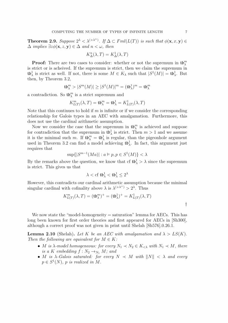
Theorem 2.9. Suppose 2λ < λ(+λ+). If ∆ ⊂ Fml(L(T )) is such that φ(x, x,y) ∈∆ implies ∃zφ(x, z,y) ∈ ∆ and n < ω, then

Kn∆(λ, T ) = K1

∆(λ, T )

Proof: There are two cases to consider: whether or not the supremum in tbmλis strict or is acheived. If the supremum is strict, then we claim the supremum intb1λ is strict as well. If not, there is some M ∈ Kλ such that |S1(M)| = tb1

λ. Butthen, by Theorem 3.2,

tbmλ > |Sm(M)| ≥ |S1(M)|m = (tb1λ)m = tbmλ

a contradiction. So tbmλ is a strict supremum and

KmL(T )(λ, T ) = tbmλ = tb1

λ = K1L(T )(λ, T )

Note that this continues to hold if m is infinite or if we consider the correspondingrelationship for Galois types in an AEC with amalgamation. Furthermore, thisdoes not use the cardinal arithmetic assumption.

Now we consider the case that the supremum in tbmλ is achieved and supposefor contradiction that the supremum in tb1

λ is strict. Then m > 1 and we assumeit is the minimal such m. If tbmλ = tb1

λ is regular, than the pigeonhole argumentused in Theorem 3.2 can find a model achieving tb1

λ. In fact, this argument justrequires that

sup{|Sm−1(Ma)| : a � p, p ∈ S1(M)} < λ

By the remarks above the question, we know that cf tb1λ > λ since the supremum

is strict. This gives us that

λ < cf tb1λ < tb1

λ ≤ 2λ

However, this contradicts our cardinal arithmetic assumption because the minimalsingular cardinal with cofinality above λ is λ(+λ+) > 2λ. Thus

KmL(T )(λ, T ) = (tbmλ )+ = (tb1

λ)+ = K1

L(T )(λ, T )

†

We now state the “model-homogeneity = saturation” lemma for AECs. This haslong been known for first order theories and first appeared for AECs in [Sh300],although a correct proof was not given in print until Shelah [Sh576].0.26.1.

Lemma 2.10 (Shelah). Let K be an AEC with amalgamation and λ > LS(K).Then the following are equivalent for M ∈ K:

• M is λ-model homogeneous: for every N1 ≺ N2 ∈ K<λ with N1 ≺M , thereis a K embedding f : N2 →N1 M ; and• M is λ-Galois saturated: for every N ≺ M with ‖N‖ < λ and everyp ∈ S1(N), p is realized in M .

8 WILL BONEY

3. Results on Sα(M)

This section aims to prove Theorem 1.1 for AECs. In our notation, this can bestated as follows.

Theorem 3.1. If K is an AEC with λ amalgamation, then for any κ ≤ λ, allowingκ to be finite or infinite, we have tbκλ = (tb1

λ)κ.

We prove this by proving a lower bound (Theorem 3.2) and an upper bound(Theorem 3.5) for tbκλ. Note that when κ = λ, this value is always the set-theoretic maximum, 2λ. However, for 1 < κ < min{χ : (tb1

λ)χ = 2λ}, this provides

new information.For readers interested in AECs beyond elementary classes, we note the use of

amalgamation for the rest of this section and for the rest of this paper. It remainsopen whether these or other bounds can be found on the number of types withoutamalgamation. One possible obstacle is that different types cannot be put together:if we assume amalgamation, then given two types p, q ∈ gS1(M), there is sometype r ∈ gS2(M) such that its first coordinate extends p and its second coordinateextends q. This will be a crucial tool in the proof of the lower bound. However,if we cannot amalgamate a model that realizes p and a model that realizes q overM , then such an extension type does not necessarily exist.

For the lower bound, we essentially “put together” all of the different types ingS1(M) as discussed above.

Theorem 3.2. Let K be an AEC with λ-AP and λ-JMP. We have tbκλ ≥ (tb1λ)κ.

In particular, given M ∈ Kλ, |gSκ(M)| ≥ |gS1(M)|κ.

Proof: We first prove the “in particular” clause and use that to prove the state-ment. Fix M ∈ Kλ and set µ = |gS1(M)|. Fix some enumeration 〈pi : i < µ〉 ofgS1(M). Then we claim that there is some M+ �M that realizes all of the typesin gS1(M).To see this, let Ni � M of size λ contain a realization of pi. Then set M0 = Mand M1 = N0. For α = β + 1, amalgamate Mβ and Nβ over M to get Mα � Mβ

and f : Nβ →M Mα; since Nβ realizes pβ ∈ S(M), f(Nβ) realizes f(pβ) = pβ. SoMα does as well. Take unions at limits. Then M+ := ∪β<αMβ realizes each typein gS1(M).Having proved the claim, we show that |gSκ(M)| ≥ µκ. For each i < µ, pickai ∈ |M+| that realizes pi. For each f ∈ κµ, set af = 〈af(i) : i < κ〉. We claim thatthe map (f ∈ κµ)→ gtp(af/M,M+) is injective, which completes the proof.To prove injectivity, note that gtp(aj/M,M+) = gtp(ak/M,M+) iff j = k. Sup-pose gtp(af/M,M+) = gtp(ag/M,M+). Then, we see that gtp(af(i)/M,M+) =gtp(ag(i)/M,M+) for each i < κ. By our above note, that means that f(i) = g(i)for every i ∈ κ = dom f = dom g. So f = g. Thus, |gSκ(M)| ≥ |κµ| = µκ, asdesired.Now we prove that tbκλ ≥ (tb1

λ)κ. This is done by separating into cases based on

COMPUTING THE NUMBER OF TYPES OF INFINITE LENGTH 9

cf (tb1λ). If cf (tb1

λ) > κ, then it is known that exponentiating to κ is continuousat tb1

λ. Stated more plainly, if X is a set of cardinals such that cf (supχ∈X χ) > κ,then

(supχ∈X

χ)κ = supχ∈X

(χκ)

Then, we compute that

(tb1λ)κ = ( sup

M∈Kλ|gS1(M)|)κ = sup

M∈Kλ(|gS1(M)|κ) ≤ sup

M∈Kλ|gSκ(M)| = tbκλ

If cf (tb1λ) ≤ κ, then we also have cf (tb1

λ) ≤ λ. By Proposition 2.7, we know thatthe supremum of tb1

λ is achieved, say by M∗ ∈ Kλ. Then

(tb1λ)κ = |gS1(M∗)|κ ≤ |gSκ(M∗)| ≤ sup

M∈Kλ|gSκ(M)| = tbκλ

†

Now we show the upper bound. We do this in two steps. First, we present the“successor step” in Theorem 3.3 to give the reader the flavor of the argument.Then Theorem 3.5 gives the full argument using direct limits.

Theorem 3.3. For any AEC K with λ-AP and any n < ω, tbnλ ≤ tb1λ.

Note that, since it includes the ‖M‖ many algebraic types, gS1(M) is alwaysinfinite, so this result could be written tbnλ ≤ (tb1

λ)n.

Proof: We prove this by induction on n < ω. The base case is tb1λ ≤ tb1

λ.Suppose tbnλ ≤ tb1

λ and set µ = tb1λ. For contradiction, suppose there is some M ∈

Kλ such that |gSn+1(M)| > µ. Then we can find distinct {pi ∈ Sn+1(M) | i < µ+}and find 〈aij | j < n+ 1〉 |= pi and Ni �M that contains each aij for j < n+ 1.

Consider {gtp(〈aij | j < n〉/M,Ni) : i < µ+} ⊂ gSn(M). By assumption, thisset has size µ. So there is some I ⊂ µ+ of size µ+ such that, for all i ∈ I,gtp(〈aij | j < n〉/M,Ni) is constant.

Fix i0 ∈ I. For any i ∈ I, the Galois types of 〈aij : j < n〉 and 〈ai0j : j < n〉 over

M are equal. Thus, there are N∗i � Ni0 and fi : Ni →M N∗i such that fi(aij) = ai0j

for all j < n and

Ni0// N∗i

M

OO

// Ni

fi

OO

commutes. Now consider the set {gtp(fi(ain)/Ni0 , N∗i ) | i ∈ I}. We have that

|I| = µ+ and |S1(Ni0)| ≤ tb1λ = µ, so there is I∗ ⊂ I of size µ+ so, for all i ∈ I∗,

gtp(fi(ain)/Ni0 , N

∗i ) is constant. Let i 6= k ∈ I∗.

Then gtp(fi(ain)/Ni0 , N

∗i ) = gtp(fk(a

kn)/Ni0 , N

∗k ). By the definition of Galois types,

10 WILL BONEY

we can find N∗∗, gk : N∗k → N∗∗, and gi : N∗i → N∗∗ such that gk(fk(akn)) =

gi(fi(ain)) and the following commutes

N∗kgk // N∗∗

Ni0

OO

// N∗i

gi

OO

We put these diagrams together and get the following:

N∗∗

N∗k

gk

<<zzzzzzzzN∗i

gi

bbDDDDDDDD

Ni0

=={{{{{{{{

aaCCCCCCCC

Nk

fk

OO

Ni

fi

OO

M

<<yyyyyyyy

bbEEEEEEEE

OO

Thus, we have amalgamatedN∗i andN∗k overM . Furthermore, for each j < n+1,we have gk(fk(a

kj )) = gi(fi(a

ij)). This witnesses gtp(〈aij | j < n + 1〉/M,Ni) =

gtp(〈ajj | j < n+ 1〉/M,Nj), which is a contradiction.

Thus, |gSn+1(M)| ≤ µ = tbλ1 for all M ∈ Kλ as desired. †

This proof can be seen as a semantic generalization of the proof that stabilityfor 1-types implies stability. Now we wish to prove this upper bound for types ofany length ≤ λ.

The proof works by induction to construct a tree of objects that is indexed by(tb1

λ)–called µ in the proof–that codes all κ length types as its branches. Successorstages of the construction are similar to the above proof, but with added book-keeping. At limit stages, we wish to continue the construction in a continuous way.However, we will have a family of embeddings rather than an increasing ≺K-chain.This is fine since the following closure under direct limits follows from the AECaxioms.

Fact 3.4. If we have 〈Mi ∈ K : i < κ〉 and, for i < j < κ, a coherent set ofembeddings fi,j : Mj → Mi—that is, one so, for i < j < k < κ, fi,k = fj,k ◦ fi,j—then there is an L(K) structure M = lim−→i<j<κ

(Mi, fi,j) and embeddings fi,∞ :

Mi → M so that, for all i < j < κ, fi,∞ = fj,∞ ◦ fi,j and, for each x ∈ M , there

COMPUTING THE NUMBER OF TYPES OF INFINITE LENGTH 11

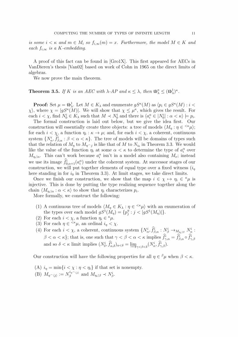
is some i < κ and m ∈ Mi so fi,∞(m) = x. Furthermore, the model M ∈ K andeach fi,∞ is a K-embedding.

A proof of this fact can be found in [Gro1X]. This first appeared for AECs inVanDieren’s thesis [Van02] based on work of Cohn in 1965 on the direct limits ofalgebras.

We now prove the main theorem.

Theorem 3.5. If K is an AEC with λ-AP and κ ≤ λ, then tbκλ ≤ (tb1λ)κ.

Proof: Set µ = tb1λ. Let M ∈ Kλ and enumerate gSκ(M) as 〈pi ∈ gSκ(M) : i <

χ〉, where χ = |gSκ(M)|. We will show that χ ≤ µκ, which gives the result. Foreach i < χ, find N i

0 ∈ Kλ such that M ≺ N i0 and there is 〈aαi ∈ |N i

0| : α < κ〉 |= pi.The formal construction is laid out below, but we give the idea first. Our

construction will essentially create three objects: a tree of models 〈Mη : η ∈ <κµ〉;for each i < χ, a function ηi : κ → µ; and, for each i < χ, a coherent, continuous

system {N iα, f

iβ,α : β < α < κ}. The tree of models will be domains of types such

that the relation of Mη to Mη_j is like that of M to Ni0 in Theorem 3.3. We wouldlike the value of the function ηi at some α < κ to determine the type of aαi overMηi�α. This can’t work because aαi isn’t in a model also containing Mν ; instead

we use its image f i0,α+1(aαi ) under the coherent system. At successor stages of ourconstruction, we will put together elements of equal type over a fixed witness (iηhere standing in for i0 in Theorem 3.3). At limit stages, we take direct limits.

Once we finish our construction, we show that the map i ∈ χ 7→ ηi ∈ κµ isinjective. This is done by putting the type realizing sequence together along thechain 〈Mηi�α : α < κ〉 to show that ηi characterizes pi.

More formally, we construct the following:

(1) A continuous tree of models 〈Mη ∈ Kλ : η ∈ <κµ〉 with an enumeration ofthe types over each model gS1(Mη) = {pηj : j < |gS1(Mη)|}.

(2) For each i < χ, a function ηi ∈ κµ.(3) For each η ∈ <κµ, an ordinal iη < χ.

(4) For each i < χ, a coherent, continuous system {N iα, f

iβ,α : N i

β →Mηi�βN iα :

β < α < κ}; that is, one such that γ < β < α < κ implies f iγ,α = f iβ,α ◦ f iγ,βand so δ < κ limit implies (N i

δ, fiα,δ)α<δ = lim−→γ<β<δ

(N iα, f

iγ,β).

Our construction will have the following properties for all η ∈ βµ when β < κ.

(A) iη = min{i < χ : η < ηi} if that set is nonempty.

(B) Mη_〈j〉 := Niη_〈j〉β and Mηi�β ≺ N i

β.

12 WILL BONEY

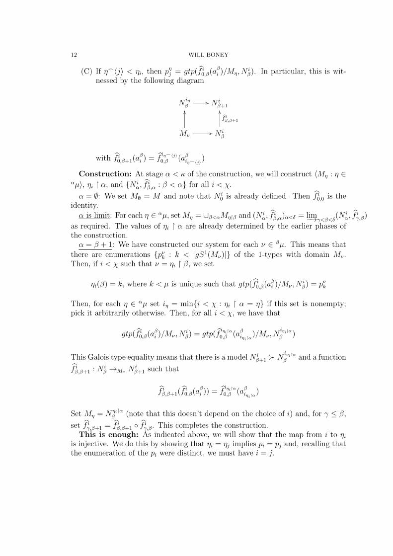
(C) If η_〈j〉 < ηi, then pηj = gtp(f i0,β(aβi )/Mη, Niβ). In particular, this is wit-

nessed by the following diagram

Niηβ

// N iβ+1

Mν

OO

// N iβ

f iβ,β+1

OO

with f i0,β+1(aβi ) = fiη_〈j〉0,β (aβiη_〈j〉)

Construction: At stage α < κ of the construction, we will construct 〈Mη : η ∈αµ〉, ηi � α, and {N i

α, fiβ,α : β < α} for all i < χ.

α = ∅: We set M∅ = M and note that N i0 is already defined. Then f i0,0 is the

identity.

α is limit: For each η ∈ αµ, setMη = ∪β<αMη�β and (N iα, f

iβ,α)α<δ = lim−→γ<β<δ

(N iα, f

iγ,β)

as required. The values of ηi � α are already determined by the earlier phases ofthe construction.α = β + 1: We have constructed our system for each ν ∈ βµ. This means that

there are enumerations {pνk : k < |gS1(Mν)|} of the 1-types with domain Mν .Then, if i < χ such that ν = ηi � β, we set

ηi(β) = k, where k < µ is unique such that gtp(f i0,β(aβi )/Mν , Niβ) = pνk

Then, for each η ∈ αµ set iη = min{i < χ : ηi � α = η} if this set is nonempty;pick it arbitrarily otherwise. Then, for all i < χ, we have that

gtp(f i0,β(aβi )/Mν , Niβ) = gtp(f

iηi�α0,β (aβiηi�α

)/Mν , Niηi�αβ )

This Galois type equality means that there is a model N iβ+1 � N

iηi�αβ and a function

f iβ,β+1 : N iβ →Mν N

iβ+1 such that

f iβ,β+1(f i0,β(aβi )) = fiηi�α0,β (aβiηi�α

)

Set Mη = Nηi�αβ (note that this doesn’t depend on the choice of i) and, for γ ≤ β,

set f iγ,β+1 = f iβ,β+1 ◦ f iγ,β. This completes the construction.This is enough: As indicated above, we will show that the map from i to ηi

is injective. We do this by showing that ηi = ηj implies pi = pj and, recalling thatthe enumeration of the pi were distinct, we must have i = j.

COMPUTING THE NUMBER OF TYPES OF INFINITE LENGTH 13

Let i, j < χ such that η := ηi = ηj. We want to show pi = pj. We have thefollowing commuting diagram of models for each β < α < κ:

N j0

fj0,�

Mη�0

��

oo // N i0

f i0,�

N jβ

fjβ,α��

Mη�β

��

oo // N iβ

f iβ,α��

N jα Mη�αoo // N i

α

with the property that, for each α < κ, we know

f i0,α+1(aαi ) = fiη�α+1

0,α (aαiη�α+1)

= f j0,α+1(aαj )

Note that this element is in Mη�α+1. Now set M = ∪α<κMη�α.

Let k stand in for either i or j. Set (Nk, fkα,∞)α<κ = lim−→γ<β<κ(Nk

β , fkγ,β). This

gives us the following diagram.

N i0

f i0,∞ ��

Moo

��

// N j0

fj0,∞ ��

N i M //oo N j

Then we can amalgamate N j and N i over M with

N j g // N∗

M //

OO

N i

f

OO

Then, for all α < κ and k = i, j, fk0,∞(aαk ) = fkα+1,∞(fk0,α+1(aαk )). We know that

fk0,α+1(aαk ) ∈ |Mη�α+1|, so it is fixed by fkβ for β > α+ 1. This means it is also fixed

by fkα+1,∞. Then

fk0,∞(aαk ) = fkα+1,∞(fk0,α+1(aαk )) = fk0,α+1(aαk ) = fiη�α+1

0,α (aαiη�α+1)

Since this last term is independent of whether k is i or j, we have f i0,∞(aαi ) =

f j0,∞(aαj ) ∈ M for all α < κ. Since our amalgamating diagram commutes over M ,

f(f i0(aαi )) = g(f j0 (aαj )).

14 WILL BONEY

Combining the above, we have

N j0

g◦fj0,∞// N∗

M

OO

// N i0

f◦f i0,∞

OO

with f ◦ f i0,∞(〈aαi | α < κ〉) = g ◦ f j0,∞(〈aαj | α < κ〉).Thus,

pi = gtp(〈aαi | α < κ〉/M,N i0) = gtp(〈aαj | α < κ〉/M,N j

0 ) = pj

Since each pk was distinct, this implies that i = j. The map i 7→ ηi is injectiveand χ ≤ µκ as desired. †

As mentioned in the Introduction, the above result gives us the proof of Theorem1.1:

Proof of Theorem 1.1: As discussed in the last section, (Mod T,≺L(T )) is anAEC with amalgamation over sets. Given a set A, passing to a model containingA can only increase the number of types. Thus, even in this case, it is enough toonly consider models when computing tb. Thus,

supA⊂M |=T,‖A‖=λ

|Sµ(A)| = tbµλ = (tb1λ)µ =

(sup

A⊂M |=T,‖A‖=λ|S1(A)|

)µ

as desired. †

After seeing this work, Alexei Kolesnikov pointed out a much simpler proof ofTheorem 3.5 for first order theories or, more generally, for AECs that are < ω typeshort over λ-sized domains1; in either case, a type of infinite length is determinedby its restrictions to finite sets of variables. Fix a type p ∈ SI(M) with I infinite.The previous comment means that the map

p 7→ Πx∈[I]<ωpx

from SI(M) to Πx∈[I]<ωSx(M) is injective. Then

|SI(M)| ≤ Πx∈[I]<ω |Sx(M)| = Πx∈[I]<ω |S1(M)|= |S1(M)||[I]<ω | = |S1(M)||I|

This is in fact a strengthening of Theorem 3.5 as in Theorem 3.2.We now examine local types in first order theories. For ∆ ⊂ Fml(L(T )), set

∆tbλκ = supM |=T,‖M‖=λ

|Sκ∆(M)|

1See [Bon].3.4 for a definition or ignore this case at no real loss

COMPUTING THE NUMBER OF TYPES OF INFINITE LENGTH 15

If ∆ = {φ}, we simply write φtbκλ. Unfortunately, there is no semantic equivalentof ∆-types, so the methods and proofs above do not transfer. For a lower bound,we can prove the following in the same way as Theorem 3.2.

Proposition 3.6. If T is a first order theory and ∆ ⊂ Fml(L(T )), then for anyκ we have that |S1

∆(A)| = µ implies that |Sκ∆(A)| ≥ µκ.

If ∆ is closed under existential quantification, the syntactic proofs of Theorem3.3 (see, for instance, [Sh:c].2) can be used to get an upper bound for ∆tbnλ whenn is finite.

Proposition 3.7. If for all φ(x, x,y) ∈ ∆, we have ∃zφ(x, z,y) ∈ ∆, then ∆tbnλ ≤∆tb1

λ for n < ω.

With this result for finite lengths, we can apply the syntactic argument aboveto conclude the following.

Proposition 3.8. If T is a first order theory and ∆ ⊂ Fml(L(T )), then for κ ≤ λ,

∆tbκλ ≤ (supn<ω

∆tbnλ)κ

In particular, if ∆ is closed under existentials as in Proposition 3.7, then ∆tbκλ ≤(∆tb1

λ)κ.

We now turn to the values of φtb for particular φ. Recall that Theorem [Sh:c].II.2.2says that T is stable iff T is λ stable for λ = λ|T | iff it is λ stable for φ types forall φ ∈ L(T ). This means that if T is unstable in λ = λ|T |, then there is some φsuch that φtb1

λ > λ. Further, suppose that sup{ψtb1λ : ψ ∈ L(T )} = λ+n for some

1 ≤ n < ω. Then, since λ+n is a successor, this supremum is acheived by someformula φλ. Then, since λ|T | = λ, we can calculate

φλtb1λ = sup

ψ∈L(T )

{ψtb1λ} ≤ tb1

λ ≤ Πψ∈L(T )(ψtb1λ) ≤ (φλtb

1λ)|T | =

= (λ+n)|T | = λ|T | · λ+n = λ+n = φλtb1λ

So φλtb1λ = tb1

λ. Thus, for all κ ≤ λ, we can use Theorems 3.6 and 3.5 to calculate

(φλtb1λ)κ ≤ φλtb

κλ ≤ tbκλ = (tb1

λ)κ = (φλtb

1λ)κ

This gives us the following result:

Theorem 3.9. Given a first order theory T , if λ is a cardinal such that λ|T | = λand sup{|S1

ψ(A)| : ψ ∈ L(T ), |A| ≤ λ} < λ+ω, then there is some φλ ∈ L(T ) suchthat, for all κ ≤ λ, tbκλ = φλtb

κλ.

Returning to general AECs, in [Sh:h].V.D.§3, Shelah considers long types oftuples enumerating a model extending the domain. In this case, any realization ofthe type is another model extending the domain that is isomorphic to the originaltuple over the domain. Thus, an upper bound on types of a certain length κalso bounds the number of isomorphism classes extending the domain by κ manyelements. More formally, we get

16 WILL BONEY

Proposition 3.10. Given M ∈ Kλ,

|{N/ ∼=M : N ∈ K,M � N, |N −M | = κ}| ≤ tbκλ

If we have an AEC with amalgamation where any extension can be brokeninto smaller extensions, this could lead to a useful analysis. Unfortunately, thisprovides us with no new information when κ = λ since 2λ = tbλλ is already thewell-known upper bound for λ-sized extensions of M and there are even first ordertheories where M � N implies |N −M | ≥ ‖M‖. Algebraically closed fields ofcharacteristic 0 are such an example.

4. Strongly Separative Types

One might hope that similar bounds could be developed for non-algebraic types.This would probably give us a finer picture of what is going on because a modelM necessarily has at least ‖M‖ many algebraic types over M , so in the stablecase, the number of non-algebraic types could, a priori, be anywhere between 0and ‖M‖; the case gS1

na(M) = ∅ only occurs in the uninteresting case that M hasno extensions.

However, as the following result shows, no such result is possible even in basic,well-understood first order cases:

Proposition 4.1. (1) Let T1 be the empty theory and M � T1. Then |S1na(M)| =

1 and |Snna(M)| = Bn for all n < ω, where Bn is the nth Bell number. Inparticular, this is finite.

(2) Let T2 = ACF0 and M � T . Then |S1na(M)| = 1 but |S2

na(M)| = ‖M‖.

Note that these examples represent the minimal and maximal, respectively, num-ber of long, nonalgebraic types given that there is only one non-algebraic type.

Proof:

(1) Let tp(a/M,N1), tp(b/M,N2) ∈ S1na(M) and, WLOG, assume ‖N1‖ ≤

‖N2‖. Then let f fix M , send a to b, and injectively map N1−M −{a} toN2 −M − {b} arbitrarily. This witenesses tp(a/M,N1) = tp(b/M,N2).Given the type of 〈an : n < k〉, the only restriction on finding a functionto witness type equality is given by which elements of the sequence arerepeated; for instance, if a 6= b, then tp(a, b/M,N) 6= tp(a, a/M,N). Thus,each type can be represented by those elements of the sequence which arerepeated. To count this, we need to know the number of partitions of n.This is given by Bell’s numbers, defined byB1 = 1 andBn+1 =

∑nk=0

(nk

)Bk.

See [Wil94].1.6.13 for a reference. Then, the number of n-types is just Bn.(2) This is an easy consequence of Steinitz’s Theorem that there is only one

non-algebraic 1-type, that of an element transcedental over the domain.Looking at 2-types, let M ∈ K and e ∈ N � M be transcendental (non-algebraic) overM . For each polynomial f ∈M [x], set pf = tp(e, f(e)/M,N).Then, for f 6= g, we have that pf 6= pg ∈ S2

na(M). Also, tp(e, π/M,N ′)

COMPUTING THE NUMBER OF TYPES OF INFINITE LENGTH 17

is distinct, where π is transcendental over M(e). This gives at least ‖M‖many 2-types.We know there are at most ‖M‖ many because the theory is stable. There-fore, the results of last section tells us that there are exactly ‖M‖2 = ‖M‖many 2-types, so there are at most ‖M‖ many non-algebraic 2-types. †

This shows that a result like Theorem 3.5 is impossible for non-algebraic types.As is evident in the proof above, especially part two, the variance in the number oftypes comes from the fact that, while the realizations of the non-algebraic type arenot algebraic over the model, they might be algebraic over each other. This meansthat even 2-types, like tp(e, 2e/A,C), that are not realized in the base model can’tbe separated: any algebraically closed field realizing the type of e must also realizethe type of 2e.

In order to get a bound on the number of these types, we want to be ableto separate the different elements of the tuples that realize the long types. Thismotivates our definition and naming of separative types below. We also introducea slightly stronger notion, strongly separative types, that allow us to not onlyseparate realizations of the type, but also gives us the ability to extend types, asmade evident in Proposition 4.6. Luckily, in the first order case and others, thesetwo notions coincide; see Proposition 4.5.

Definition 4.2.(1) We say that a triple (〈ai : i < α〉,M,N) ∈ K3,α

λ is separative iff there areincreasing sequences of intermediate models 〈Ni ∈ K : i < α〉 such that,for all i < α, M ≺ Ni ≺ N and ai ∈ Ni+1 −Ni. The sequence 〈Ni : i < α〉is said to witness the triple’s separativity.

(2) For M ∈ K, set gSαsep(M) = {gtp(〈ai : i < α, 〉/M,N) : (〈ai : i <

α, 〉,M,N) ∈ K3,αλ is separative}.

(3) We say that a triple (〈ai : i < α〉,M,N) ∈ K3,αλ is strongly separative iff

there is a sequence witnessing its separativity 〈Ni : i < α〉 that further hasthe property that, for any i < α and N+

1 � Ni of size λ, there is someN+

2 � N+1 and g : Ni+1 →Nβ N

+2 such that g(ai) /∈ N+

1 .(4) For M ∈ Kλ, set gSαstrsep(M) = {gtp(〈ai : i < α, 〉/M,N) : (〈ai : i <

α, 〉,M,N) ∈ K3,αλ is strongly separative}.

The condition “ai ∈ Ni+1 −Ni” in (1) could be equivalently stated as either ofthe following:

• For all j < α, aj ∈ Ni iff i < j.• gtp(ai/Ni, Ni+1) is nonalgebraic.

Note that the examples in Proposition 4.1 only have one separative or stronglyseparative type of any length: for the empty theory, this is any sequence of distinctelements and, for ACF0, this is any sequence of mutually transcendental elements.

18 WILL BONEY

Theorem 4.8 below shows this generally by proving the upper bound from the lastsection (Theorem 3.5) holds for strongly separative types. Before this proof, a fewcomments about these definitions are in order.

First, the key part of the definition is about triples, but we will prove thingsabout types. This is not an issue because any triple realizing a (strongly) separativetype can be made into a (strongly) separative type by extending the ambient model.

Proposition 4.3.(1) If gtp(〈aβ : β < α〉/M,N) ∈ gSαsep(M), then there is some N+ � N such

that (〈aβ : β < α〉,M,N+) is separative.(2) The same is true for strongly separative types.

Proof: We will prove the first assertion and the second one follows similarly.By the definition of gSαsep, there is some separative (〈bβ : β < α〉,M,N1) ∈ K3,α

λ

such that gtp(〈aβ : β < α〉/M,N) = gtp(〈bβ : β < α〉/M,N). Thus, there existssome N+ � N and f : N1 →M N+ such that f(bβ) = aβ for all β < α. Let〈Nβ : β < α〉 be a witness sequence to (〈bβ : β < α〉,M,N1)’s separativity. Then〈f(Nβ) ≺ N+ : β < α〉 is a witness sequence for (〈aβ : β < α〉,M,N+). †

Second, although we continue to use the semantic notion of types (Galois types)for full generality, these notions are new in the context of first order theories. In thiscontext, the elements of the witnessing sequence 〈Ni : i < α〉 are still required tobe models, even though types are meaningful over sets. An attempt to characterizethese definitions in a purely syntactical nature (i.e. by only mentioning formulas)was unsuccessful, but we do know (see Proposition 4.5 below) that all separativetypes over models are strongly separative for complete first order theories.

Third, we can easily characterize these properties for 1-types.

Proposition 4.4. Let K be an AEC and p ∈ gS1(M).

• p is separative iff p is nonalgebraic.• p is strongly separative iff, for any N � M with ‖N‖ = ‖M‖, there is an

extension of p to a non-algebraic type over N . Such types are called big.

Finally, strongly separative types and separative types are the same in the pres-ence of the disjoint amalgamation property.

Proposition 4.5. Let α be an ordinal and M ∈ K. If K satisfies the disjointamalgamation property when all models involved have sizes between ‖M‖ and |α|+‖M‖, inclusive, then gSαstrsep(M) = gSαsep(M).

Proof: By definition, gSαstrsep(M) ⊂ gSαsep(M), so we wish to show the othercontainment. Let gtp(〈aβ : β < α〉/M,N) ∈ gSαsep(M). Let 〈Nβ : β < α〉 be a

witnessing sequence and let N+1 � Nβ0 of size ‖Nβ0‖ for some β0 < α. By renaming

elements, we can find some copy of N+1 that is disjoint from Nβ0+1 except for Nβ0 .

COMPUTING THE NUMBER OF TYPES OF INFINITE LENGTH 19

So there are N and f : N+1∼=Nβ0

N such that N ∩Nβ0+1 = Nβ0 . Then, we can use

disjoint amalgamation on N and Nβ0+1 over Nβ0 to get N∗ and g : Nβ0+1 → N∗ so

N+1

f // N // N∗

Nβ0

aaBBBBBBBB

OO

// Nβ0+1

g

OO

commutes and N ∩ g(Nβ0+1) = Nβ0 . Thus, since aβ0 is in Nβ0+1 and not in Nβ0 ,

we have that g(aβ0) is in g(Nβ0+1) and not in N . Let f be an L(K)-isomorphismthat extends f and has N∗ in its range. Then we have

f−1(g(aβ0)) 6∈ f−1(N) = f−1(N) = N+1

Then we can collapse the above diagram to

N+1

// f−1(N∗)

Nβ0

OO

// Nβ0+1

f−1◦g

OO

This diagram commutes and witnesses the property for strong separativity with

N+2 = f−1(N∗). †

It is an exercise in the use of compactness that every complete first order the-ory satisfies disjoint amalgamation over models, see Hodges [Hod93].6.4.3 for areference. For a general AEC, this is not the case. Baldwin, Kolesnikov, andShelah [BKSh927] have constructed examples of AECs without disjoint amalga-mation. On the other hand, Shelah [Sh576] has shown that disjoint amalgamationfollows from certain amounts of structure (see, in particular, 2.17 and 5.11 there).Additionally, Grossberg, VanDieren, and Villaveces [GVV] point out that manyAECs with a well developed independence notion, such as homogeneous modeltheory or finitary AECs, also satisfy disjoint amalgamation.

In order to prove the main theorem of this section, Theorem 4.8, we will needto make use of certain closure properties of strongly separative types. These alsohold for separative types as well.

Proposition 4.6 (Closure of gSstrsep).

(1) If p ∈ gSαstrsep(M) and I ⊂ α, then pI ∈ gSotp(I)strsep(M).(2) If p ∈ gSαstrsep(M) and M0 ≺M , then p �M0 ∈ gSαstrsep(M0).

We now prove the main theorem.

Definition 4.7. The strongly separative type bound for λ sized domains and κlengths is denoted strseptbκλ = supM∈Kλ |gS

κstrsep(M)|.

20 WILL BONEY

Theorem 4.8. If strseptb1λ = µ, then strseptbκλ ≤ µκ for all (possibly finite)

κ ≤ λ+.

Proof: The proof is very similar to that of Theorem 3.5, so we only highlightthe differences.

As before, let M ∈ Kλ, enumerate gSκstrsep(M) = 〈pi : i < χ〉, and find N i0 �M

of size λ+ κ and aαi ∈ |N i0| for i < χ and α < κ such that 〈aαi : α < κ〉 � pi.

Then, we use strong separativity to find a witnessing sequence. That is, for eachi < χ, we have increasing and continuous 〈αN i

0 ∈ Kλ : α < κ〉 so, for each α < κ,M ≺ αN i

0 ≺ N i0 and aαi ∈ α+1N i

0 − αN i0.

As before, we will construct 〈Mη ∈ Kλ : η ∈ <κµ〉, 〈pηj ∈ gS1strsep(Mη) : j <

|gS1strsep(Mη)|〉, 〈iη ∈ χ : η ∈ <κµ〉, and 〈ηi ∈ κµ : i < χ〉 as in (1) − (3) of the

proof of Theorem 3.5 and

(4*) For i < χ, a coherent, continuous {αN iα, f

iβ,α : βN i

β →Mηi�βαN i

α | β < α <

κ}, models 〈α+1N iα : α < κ〉, and, for each β < α < κ, functions

• hiα : αN i0 → αN i

α;• giβ+1 : β+1N i

0 → β+1N iβ; and

• f iβ+1 : β+1N iβ →Mηi�β

βN iβ.

These will satisfy (A), (B), and (C) from Theorem 3.5 and

(D) If α = β + 1, then hiα = f iα ◦ giα and, if α is limit, then αN iα is the direct

limit and, for each δ < α, the following commutes

δN iδ

f iδ,α // αN iα

δN i0

hiδ

OO

// αN i0

hiα

OO

(E) If α < κ, then• hiα � αN i

0 = giα+1 �αN i

0

• giα+1(aαi ) 6∈ αN iα

• hiα+1(aαi ) = giηi�αα+1 (aαiηi�α

)

• f iα,α+1 = f iα+1

Construction:The base case and limit case are the same as in 3.5. In the limit, we additionally

set hiα =⋃β<α h

iβ.

For `(η) = α = β + 1 we will apply our previous construction to the separatingmodels. Fix some ν ∈ βµ. For each i < χ such that ηi � β = ν, we havehiβ : βN i

0 → βN iβ. We know that gtp(aβi /

βN i0,β+1N i

0) is big by Propositions 4.6 and

4.4. Thus we can find a big extension with domain (hiβ)−1(βN iβ). Then, applying

COMPUTING THE NUMBER OF TYPES OF INFINITE LENGTH 21

hiβ to this type, we get some giβ+1 : β+1N i0 → β+1N i

β so

βN iβ

// β+1N iβ

βN i0

hiβ

OO

// β+1N i0

giβ+1

OO

commutes and gtp(giβ+1(aβi )/Mν ,β+1N i

β) is big and, therefore, strongly separative.Note that this extension uses that these types are strongly separative and not justseparative. Then we can extend ηi by ηi(β) = k where k < µ is the unique index

such that gtp(giβ+1(aβi )/Mν ,β+1N i

β) = pνk.Then set iν_〈i〉 = min{i < χ : ηi � α = ν_〈i〉}. This means that, for all i < χ, wehave

gtp(giβ+1(aβi )/Mν ,β+1N i

β) = gtp(giηi�αβ+1 (aβiηi�α

)/Mν ,β+1N

iηi�αβ )

Thus, we can find β+1N iβ+1 � β+1N

iηi�αβ from Kλ and f iβ+1 : β+1N i

β →Mνβ+1N i

β+1

such that f iβ+1(giβ+1(aβi )) = giηi�αβ+1 (aβiηi�α

). Finally, set Miηi�α= β+1N

iηi�αβ and hiβ+1 =

f iβ+1 ◦ giβ+1.This is enough: For each i < χ and every α < β < κ, we have

Mη�0//

��

0N i0

//

f i0,�

βN i0

//

hiβ}}{{{{{{{{

αN i0

//

hiα

}}{{{{{{{{{{{{{{{{{{{{{{

N i0

Mη�β

��

// βN iβ

f iβ,α��

Mη�α// αN i

α

that commutes. Note that this is almost the same diagram as before, except wehave added the separating sequences. Then we can proceed as before, setting

(1) M = ∪α<κMη�α;

(2) (N i, fα,∞) = lim−→β<γ<κ(βN i

β, fiα,β);

(3) N i1 = ∪α<καN i

0 ≺ N i0.

(4) fi : N i1 → N i by fi = ∪α<κ(fα,∞ ◦ hiα); and

(5) ηi ∈ κµ such that i ∈ Iη�α for all α < κ.

Then, if χ > µκ, there are i 6= j such that ηi = ηj. As before, this would implypi = pj, but they are all distinct. So χ ≤ µκ as desired. †

In the previous theorem, we allowed the case κ = λ+. Most of the time, this is

only the set-theoretic bound strseptbλ+

λ ≤ 2λ+

. However, if we had strseptb1λ = 1,

then we get the surprising result that strseptbλ+

λ ≤ 1. This will be explored along

22 WILL BONEY

with further investigation of classifying AECs based on separative types in futurework.

5. Saturation

We now turn from the number of infinite types to their realizations. The satu-ration version of Theorem 3.1 is much simpler to prove.

Proposition 5.1. If M ∈ Kλ is Galois saturated for 1-types, then M is Galoissaturated for λ-types.

Proof: Let M0 ≺ M of size < λ and p ∈ gSλ(M0). By the definition of Galoistypes, there is some N � M0 of size λ that realizes p. Find a resolution of N〈Ni ∈ K<λ | i < cf λ〉 with N0 = M0. Then use Lemma 2.10 to get increasing,continuous fi : Ni →M that fix M0. Then f := ∪i<λfi : N →M0 M . This impliesf(N) |= f(p) = p and since f(N) ≺M , M |= p. †

We can get a parameterized version with the same proof.

Proposition 5.2. If M ∈ Kλ is µ-Galois saturated for 1-types, then M is µ-Galoissaturated for µ-types.

The seeming simplicity of the proof of Proposition 5.1, especially compared toearlier uses of direct limits, hides the difficulty and complexity of the proof ofLemma 2.10. Although the statement is a generalization of a first order fact, itsannouncement was a surprise and many flawed proofs were proposed before a suc-cessful proof was given. Building on work of Shelah, Grossberg, and Kolesnikov,Baldwin [Bal09].16.5 proves a version of Lemma 2.10 which does not require amal-gamation. This gives rise to a version of Proposition 5.1 in AECs even withoutamalgamation.

There is also a strong relationship between the value of tb1λ and the existence of

λ+-saturated extensions of models of size λ. The following generalizes first ordertheorems like [Sh:c] Theorem VIII.4.7.

In the following theorems, we make use of a monster model, as in first ordermodel theory, to reduce the complexity of constructions. Full details can be foundin the references given at the start of Section 2, but the key facts are

• the existence of a monster model C follows from the amalgamation prop-erty, the joint embedding property, and every model having a proper ≺K-extension; and• for M ≺ C and a, b ∈ |C|,

gtp(a/M) = gtp(b/M) ⇐⇒ ∃f ∈ AutMC so f(a) = b

The first relationship is clear from counting types.

Theorem 5.3. Let K be an AEC with amalgamation, joint embedding, and nomaximal models. If every M ∈ Kκ has an extension N ∈ Kλ that is κ+-saturated,then tb1

κ ≤ λ.

COMPUTING THE NUMBER OF TYPES OF INFINITE LENGTH 23

Proof: Assume that every model in Kκ has a κ+-saturated extension of size λ.Let M ∈ Kκ and N ∈ Kλ be that extension. Since every type over M is realizedin N , we have |gS(M)| ≤ ‖N‖ = λ. Taking the sup over all M ∈ Kκ, we gettb1κ ≤ λ, as desired. †Going the other way, we have both a set theoretic hypothesis and model theoretic

hypothesis that imply instances of a κ+-saturated extension. The set-theoreticversion is well known.

Theorem 5.4. Let K be an AEC with amalgamation, joint embedding, and nomaximal models. If λκ = λ, then every M ∈ Kκ has an extension N ∈ Kλ that isκ+ saturated.

Note that the hypothesis implies tb1λ ≤ λ. Without this set theoretic hypothesis,

reaching our desired conclusion is much harder. λκ = λ means that we can con-sider all κ size submodels of a λ sized model without going up in size. Without thisassumption, things become much more difficult and we must rely on model the-oretic hypotheses. The following has a stability-like hypothesis, sometimes called‘weak stability;’ see [JrSh875], for instance.

Theorem 5.5. Let K be an AEC with amalgamation, joint embedding, and nomaximal models. If tb1

κ ≤ κ+, then every M ∈ Kκ has an extension N ∈ Kκ+ thatis saturated.

Proof: We proceed by a series of increasingly strong constructions.Construction 1: For all M ∈ Kκ, there is M∗ ∈ Kκ+ such that all of S1(M) isrealized in M∗.This is easy with |S1(M)| ≤ κ+.Construction 2: For all M ≺ N from Kκ and M ≺ M ′ ∈ Kκ+ , there is someN ′ = ∗(M,N,M ′) ∈ Kκ+ such that N,M ′ ≺ N ′ and all of S1(N) are realized inN ′.For each p ∈ S1(N), find some ap ∈ |C| that realizes it. Then find some N ′ ≺ Cthat contains {ap : p ∈ S1(N)} ∪ |M ′| ∪ |N | of size κ+. This is possible since|S1(N)| ≤ κ+.Construction 3: For all M ∈ Kκ+ there is some M+ ∈ Kκ+ such that M ≺M+

and, if M0 ≺M of size κ, then all of S1(M0) are realized in M+.Find a resolution 〈Mi : i < κ+〉 of M . Set N0 = (M0)∗, Ni+1 = ∗(Mi,Mi+1, Ni),and take unions at limits. Then M+ = ∪i<κ+Ni works.Construction 4: For all M ∈ Kκ+ , there is some M# ∈ Kκ+ such that M ≺M#

and M# is saturated.Let M ∈ Kκ. Set M0 = M , Mi+1 = (Mi)

+, and take unions at limits. ThenM# = Mκ+ is saturated.Then, to prove the proposition, let M ∈ Kκ. Since K has no maximal model, ithas an extension M ′ in Kκ+ . Then (M ′)# is the desired saturated extension of M .†

24 WILL BONEY

6. Further Work

In working with Galois types, as we do here, the assumption of amalgamationsimplifies the definitions and construction by making EAT already an equivalencerelation in the definition of types; see Definition 2.4. Could we obtain some boundon the number of long types in the absence of amalgamation?

In this paper, we introduced the definitions of Ssep and Sstrsep. There are severalbasic questions to explore.

First, is Sstrsep necessary? That is, is there an AEC where the size of Sstrsepis well behaved, but Ssep is chaotic as in Proposition 4.1; or can the proof ofTheorem 4.8 be improved to provide the same bound on seqtb? By Proposition4.5, any example of this chaotic behavior must have amalgamation but not disjointamalgamation. Perhaps one of the examples from [BKSh927] can be refined forthis purpose.

In the original definitions of separative and strongly separative types, any or-dered set I was allowed as an index set and the separation properties were requiredto hold for all subsets instead of just an initial segment. We give the original defini-tion here under the names unordered separative and unordered strongly separativetypes.

Definition 6.1.(1) For M ∈ K, define gSαusep(M) = {gtp(〈ai : i ∈ I〉/M,N) ∈ gSIna(M) :

for all I0 ⊂ I, there is some M ≺ NI0 ≺ N such that ai ∈ NI0 iff i ∈ I0}.(2) For M ∈ K, define gSIustrsep(M) = {p = gtp(〈ai : i ∈ I〉/M,N) ∈

gSIusep(M) : for all I0 ⊂ I and M ≺ NI0 ≺ N , if with ai ∈ NI0 iff i ∈ I0,

then for every f : NI0 → N+1 with ‖N+

1 ‖ = NI0, there is some g : N → N+2

such that f ⊂ g and g(〈ai : i ∈ I − I0〉) 6∈ N+1 }.

Are these definitions equivalent to the ones given in Section 4, or is there someexample of an AEC where the two notions are distinct? This question will likelybe clarified by a lower bound for strseptb or an example lacking amalgamation.

A more lofty goal would be to attempt to classify stable, DAP AECs by thepossible values of natb1

λ = septb1λ. That is, we know that natb1

λ is a cardinalbetween 1 and λ and that this controls the value of septbκλ for all κ ≤ λ. Foreach value in [1, λ]∩CARD, does an AEC with DAP and exactly that many non-algebraic types of length one exist? Of particular interest is the discussion afterTheorem 4.8. The conclusion of only one separative type (or strongly separativetype, if we wish to drop the assumption of DAP) of any length over a model seemsto be a very powerful hypothesis.

Looking back to the first order case, it would be interesting to find a syntacticcharacterization of separative types, keeping in mind that separative and stronglyseparative types are equivalent in this context.

COMPUTING THE NUMBER OF TYPES OF INFINITE LENGTH 25

References

[Bal07] John Baldwin, Generalized quantifiers, infinitary logics, and abstract elementaryclasses, Proceedings of Mostowski Conference (2007).

[Bal09] , Categoricity, University Lecture Series, American Mathematical Society,2009.

[BET07] John Baldwin, Paul Ekloff, and J. Trlifaj, ⊥N as an abstract elementary class, Annalsof Pure and Applied Logic 149 (2007), 25–39.

[BK09] John Baldwin and Alexei Kolesnikov, Categoricity, amalgamation, and tameness, IsraelJournal of Mathematics 170 (2009), no. 1, 411–443.

[BKSh927] John Baldwin, Alexei Kolesnikov, and Saharon Shelah, The amalgamation spectrum,Journal of Symbolic Logic 74 (2009), 914–928.

[BG] Will Boney and Rami Grossberg, Forking in short and tame AECs, Submitted,http://www.math.cmu.edu/~wboney/BoneyGrossbergNFShortTame.pdf.

[Bon] , Tameness from large cardinals axioms, Accepted, Journal of Symbolic Logic,http://www.math.cmu.edu/~wboney/BoneyTameLC.pdf.

[Gro02] Rami Grossberg, Classification theory for abstract elementary classes, Logic and Alge-bra (Yi Zhang, ed.), vol. 302, American Mathematical Society, 2002, pp. 165–204.

[Gro1X] , A Course in Model Theory, In Preparation, 201X.[GV06a] Rami Grossberg and Monica VanDieren, Categoricity from one successor cardinal in

tame abstract elementary classes, Journal of Mathematical Logic 6 (2006), no. 2, 181–201.

[GV06b] , Galois-stability for tame abstract elementary classes, Journal of MathematicalLogic 6 (2006), no. 1, 25–49.

[GVV] Rami Grossberg, Monica VanDieren, and Andres Villaveces, Unique-ness of limit models in abstract elementary classes, Submitted,http://www.math.cmu.edu/~rami/GVV_1_12_2012.pdf

[HaSh323] Brad Hart and Saharon Shelah, Categoricity over P for first order T or categoricityfor φ ∈ Lω1ω can stop at ℵk while holding for ℵ0, · · · ,ℵk−1, Israel Journal of Mathe-matics 70 (1990), 219–235.

[Hod93] Wilfrid Hodges, Model Theory, Cambridge University Press, 1993.[JrSh875] Adi Jarden and Saharon Shelah, Non-forking frames in abstract elementary classes,

Annals of Pure and Applied Logic 164 (2013), no. 3, 135–191.[Kei70] H. Jerome Keisler, Logic with the quantifier “there exist uncountably many”, Annals of

Mathematical Logic 1 (1970), 1–93.[Kei71] , Model Theory for Infinitary Logic, Studies in Logic and the Foundations

of Mathematics, vol. 62, North-Holland Publishing Co., Amsterdam, 1971.[Kei76] , Six classes of theories, Journal of the Australian Mathematical Society 21

(1976), 257–266.[MaSh285] Michael Makkai and Saharon Shelah, Categoricity of theories in Lκω, with κ a com-

pact cardinal, Annals of Pure and Applied Logic 47 (1990), 41–97.[Pil83] Anand Pillay, An Introduction to Stability Theory, Dover Publications, Inc, 1983.[Sh:c] Saharon Shelah, Classification theory and the number of nonisomorphic mod-

els, 2nd ed., vol. 92, North-Holland Publishing Co., Amsterdam, xxxiv+705 pp, 1990.[Sh:h] , Classification Theory for Abstract Elementary Classes, vol. 1 & 2,

Mathematical Logic and Foundations, no. 18 & 20, College Publications, 2009.[Sh88] , Classification of nonelementary classes, II. Abstract elementary classes, Clas-

sification theory (John Baldwin, ed.), 1987, pp. 419–497.[Sh300] , Universal classes, Classification theory (John Baldwin, ed.), 1987, pp. 264–418.

26 WILL BONEY

[Sh576] , Categoricity of an abstract elementary class in two successive cardinals, IsraelJournal of Mathematics (2001), no. 126, 29–128.

[Van02] Monica VanDieren, Categoricity and Stability in Abstract Elementary Classes, PhDthesis, 2002.

[Wil94] Herbert S. Wilf, Generatingfunctionology, Academic Press, Inc, 1994.

E-mail address: wboney@cmu.edu

Department of Mathematical Sciences, Carnegie Mellon University, Pitts-burgh, Pennsylvania, USA