Computing in Finance – C++ Project

Terreneuve-devel Project

Simon LEGERAloke MUKHERJEE

Joseph PEREZYann RENOUX

December 22, 2005

Abstract

Welcome to Terreneuve.What is Terreneuve? Simply: ”A lightweight C++ library for quantitative finance applications”.In more detail, Terreneuve is our team name for the project in the Fall 2005 Computing in Finance course

at NYU’s Courant Institute Masters in Math Finance. Working from this specification we hope to design auseable C++ library for some important quantitative finance applications.

Our target audience (aside from our prof ;-)) is students in quantitative finance and those seeking a gentleintroduction to financial computing. Obviously, we also intend to use the project as a learning opportunity. Werefer those looking for a more comprehensive (and complex) library to the quantlib project.

Also...why Terreneuve? Well, we’re three Frenchmen and one Canadian, so we picked something a littleFrench and a little Canadian. Terreneuve is French for ”Newfoundland”, one of Canada’s provinces, as well assignifying the new world we’re exploring with this project.

- the Terreneuve team 1

1We would like to thank our parents, our grand parents, and ... wait a minute, are we supposed to make this a seriouspage ?Many thanks to the nerds that invented the Internet, we used it a lot. We are also thankful to sourceforge.net for theuser-friendly interface to share code and use it with CVS, it helped a lot.Last, but not least we would like to thank Kishor Laud for all the answers he provided during the development of thisproject, and all our classmates for asking so many questions that Kishor often answered the ones we would ask ourselveseven before we thought about them.

Contents

1 Introduction 51.1 Why, where, when, what for... Terreneuve reason for life . . . . . . . . . . . . . . . . . 51.2 Design . . . . . . . . . . . . . . . . . . . . . . . . . . . . . . . . . . . . . . . . . . . . 51.3 Approach . . . . . . . . . . . . . . . . . . . . . . . . . . . . . . . . . . . . . . . . . . . 51.4 Choices . . . . . . . . . . . . . . . . . . . . . . . . . . . . . . . . . . . . . . . . . . . . 61.5 Project Management . . . . . . . . . . . . . . . . . . . . . . . . . . . . . . . . . . . . . 61.6 Interface and Testing . . . . . . . . . . . . . . . . . . . . . . . . . . . . . . . . . . . . . 7

2 User Interface 82.1 Requirements . . . . . . . . . . . . . . . . . . . . . . . . . . . . . . . . . . . . . . . . . 82.2 Main . . . . . . . . . . . . . . . . . . . . . . . . . . . . . . . . . . . . . . . . . . . . . 82.3 Import . . . . . . . . . . . . . . . . . . . . . . . . . . . . . . . . . . . . . . . . . . . . 92.4 Products . . . . . . . . . . . . . . . . . . . . . . . . . . . . . . . . . . . . . . . . . . . . 92.5 Portfolio . . . . . . . . . . . . . . . . . . . . . . . . . . . . . . . . . . . . . . . . . . . . 102.6 Credits . . . . . . . . . . . . . . . . . . . . . . . . . . . . . . . . . . . . . . . . . . . . . 102.7 Quit . . . . . . . . . . . . . . . . . . . . . . . . . . . . . . . . . . . . . . . . . . . . . . 10

3 Common objects 113.1 Date class . . . . . . . . . . . . . . . . . . . . . . . . . . . . . . . . . . . . . . . . . . . 11

3.1.1 Approach . . . . . . . . . . . . . . . . . . . . . . . . . . . . . . . . . . . . . . . 113.1.2 Implementation . . . . . . . . . . . . . . . . . . . . . . . . . . . . . . . . . . . . 11

3.2 Interpolator . . . . . . . . . . . . . . . . . . . . . . . . . . . . . . . . . . . . . . . . . . 113.2.1 Approach . . . . . . . . . . . . . . . . . . . . . . . . . . . . . . . . . . . . . . . 113.2.2 Implementation . . . . . . . . . . . . . . . . . . . . . . . . . . . . . . . . . . . . 12

3.3 Matrix . . . . . . . . . . . . . . . . . . . . . . . . . . . . . . . . . . . . . . . . . . . . . 123.3.1 Approach . . . . . . . . . . . . . . . . . . . . . . . . . . . . . . . . . . . . . . . 123.3.2 Implementation . . . . . . . . . . . . . . . . . . . . . . . . . . . . . . . . . . . . 12

3.4 Cummulative bivariate normal distribution . . . . . . . . . . . . . . . . . . . . . . . . 133.4.1 Approach . . . . . . . . . . . . . . . . . . . . . . . . . . . . . . . . . . . . . . . 133.4.2 Results and effects of the correlation . . . . . . . . . . . . . . . . . . . . . . . . 13

3.5 FileReader . . . . . . . . . . . . . . . . . . . . . . . . . . . . . . . . . . . . . . . . . . . 153.5.1 Approach . . . . . . . . . . . . . . . . . . . . . . . . . . . . . . . . . . . . . . . 153.5.2 Implementation . . . . . . . . . . . . . . . . . . . . . . . . . . . . . . . . . . . . 15

4 Part A: Black-Scholes and Monte Carlo pricer 164.1 Requirements . . . . . . . . . . . . . . . . . . . . . . . . . . . . . . . . . . . . . . . . . 164.2 Design . . . . . . . . . . . . . . . . . . . . . . . . . . . . . . . . . . . . . . . . . . . . 164.3 Approach . . . . . . . . . . . . . . . . . . . . . . . . . . . . . . . . . . . . . . . . . . . 174.4 Choices . . . . . . . . . . . . . . . . . . . . . . . . . . . . . . . . . . . . . . . . . . . . 174.5 Unit tests . . . . . . . . . . . . . . . . . . . . . . . . . . . . . . . . . . . . . . . . . . . 18

1

4.6 Performance . . . . . . . . . . . . . . . . . . . . . . . . . . . . . . . . . . . . . . . . . . 184.7 Validation . . . . . . . . . . . . . . . . . . . . . . . . . . . . . . . . . . . . . . . . . . . 18

5 Part B: Yield Curve 205.1 Requirements . . . . . . . . . . . . . . . . . . . . . . . . . . . . . . . . . . . . . . . . . 20

5.1.1 Other methods we added for risk management purposes . . . . . . . . . . . . . 205.1.2 From swap rates to ZC rates . . . . . . . . . . . . . . . . . . . . . . . . . . . . 21

5.2 Design . . . . . . . . . . . . . . . . . . . . . . . . . . . . . . . . . . . . . . . . . . . . 225.2.1 Approach . . . . . . . . . . . . . . . . . . . . . . . . . . . . . . . . . . . . . . . 225.2.2 Choices . . . . . . . . . . . . . . . . . . . . . . . . . . . . . . . . . . . . . . . . 225.2.3 Methods . . . . . . . . . . . . . . . . . . . . . . . . . . . . . . . . . . . . . . . . 225.2.4 Unit tests . . . . . . . . . . . . . . . . . . . . . . . . . . . . . . . . . . . . . . . 225.2.5 Performance . . . . . . . . . . . . . . . . . . . . . . . . . . . . . . . . . . . . . 25

5.3 Validation . . . . . . . . . . . . . . . . . . . . . . . . . . . . . . . . . . . . . . . . . . . 255.3.1 Approach . . . . . . . . . . . . . . . . . . . . . . . . . . . . . . . . . . . . . . . 25

6 Part C: Asset 266.1 Requirements . . . . . . . . . . . . . . . . . . . . . . . . . . . . . . . . . . . . . . . . . 266.2 Design . . . . . . . . . . . . . . . . . . . . . . . . . . . . . . . . . . . . . . . . . . . . 266.3 Approach . . . . . . . . . . . . . . . . . . . . . . . . . . . . . . . . . . . . . . . . . . . 276.4 Methods . . . . . . . . . . . . . . . . . . . . . . . . . . . . . . . . . . . . . . . . . . . . 276.5 Unit tests . . . . . . . . . . . . . . . . . . . . . . . . . . . . . . . . . . . . . . . . . . . 276.6 Performance . . . . . . . . . . . . . . . . . . . . . . . . . . . . . . . . . . . . . . . . . . 286.7 Validation . . . . . . . . . . . . . . . . . . . . . . . . . . . . . . . . . . . . . . . . . . . 28

7 Part E: Implied volatility surface 297.1 Requirements . . . . . . . . . . . . . . . . . . . . . . . . . . . . . . . . . . . . . . . . . 297.2 Design . . . . . . . . . . . . . . . . . . . . . . . . . . . . . . . . . . . . . . . . . . . . 297.3 Approach . . . . . . . . . . . . . . . . . . . . . . . . . . . . . . . . . . . . . . . . . . . 297.4 Choices . . . . . . . . . . . . . . . . . . . . . . . . . . . . . . . . . . . . . . . . . . . . 297.5 Methods . . . . . . . . . . . . . . . . . . . . . . . . . . . . . . . . . . . . . . . . . . . . 307.6 Unit tests . . . . . . . . . . . . . . . . . . . . . . . . . . . . . . . . . . . . . . . . . . . 307.7 Performance . . . . . . . . . . . . . . . . . . . . . . . . . . . . . . . . . . . . . . . . . . 307.8 Validation . . . . . . . . . . . . . . . . . . . . . . . . . . . . . . . . . . . . . . . . . . . 31

7.8.1 Approach . . . . . . . . . . . . . . . . . . . . . . . . . . . . . . . . . . . . . . . 31

8 Part F: Credit Curve 328.1 Requirements . . . . . . . . . . . . . . . . . . . . . . . . . . . . . . . . . . . . . . . . . 328.2 Design . . . . . . . . . . . . . . . . . . . . . . . . . . . . . . . . . . . . . . . . . . . . 328.3 Choices . . . . . . . . . . . . . . . . . . . . . . . . . . . . . . . . . . . . . . . . . . . . 338.4 Unit tests . . . . . . . . . . . . . . . . . . . . . . . . . . . . . . . . . . . . . . . . . . . 358.5 Performance . . . . . . . . . . . . . . . . . . . . . . . . . . . . . . . . . . . . . . . . . . 378.6 Validation . . . . . . . . . . . . . . . . . . . . . . . . . . . . . . . . . . . . . . . . . . . 37

8.6.1 Approach . . . . . . . . . . . . . . . . . . . . . . . . . . . . . . . . . . . . . . . 37

9 Part D: IR Vanilla Swap 409.1 Requirements . . . . . . . . . . . . . . . . . . . . . . . . . . . . . . . . . . . . . . . . . 409.2 Design . . . . . . . . . . . . . . . . . . . . . . . . . . . . . . . . . . . . . . . . . . . . 409.3 Approach . . . . . . . . . . . . . . . . . . . . . . . . . . . . . . . . . . . . . . . . . . . 409.4 Choices . . . . . . . . . . . . . . . . . . . . . . . . . . . . . . . . . . . . . . . . . . . . 409.5 Unit tests . . . . . . . . . . . . . . . . . . . . . . . . . . . . . . . . . . . . . . . . . . . 41

2

9.6 Validation . . . . . . . . . . . . . . . . . . . . . . . . . . . . . . . . . . . . . . . . . . . 419.6.1 Approach . . . . . . . . . . . . . . . . . . . . . . . . . . . . . . . . . . . . . . . 419.6.2 Pitfalls . . . . . . . . . . . . . . . . . . . . . . . . . . . . . . . . . . . . . . . . . 41

10 Part H: Treasury Bonds/Risky Bonds 4210.1 Requirements . . . . . . . . . . . . . . . . . . . . . . . . . . . . . . . . . . . . . . . . . 4210.2 Design . . . . . . . . . . . . . . . . . . . . . . . . . . . . . . . . . . . . . . . . . . . . 4210.3 Choices . . . . . . . . . . . . . . . . . . . . . . . . . . . . . . . . . . . . . . . . . . . . 4210.4 Methods . . . . . . . . . . . . . . . . . . . . . . . . . . . . . . . . . . . . . . . . . . . . 4210.5 Unit tests . . . . . . . . . . . . . . . . . . . . . . . . . . . . . . . . . . . . . . . . . . . 4310.6 Performance . . . . . . . . . . . . . . . . . . . . . . . . . . . . . . . . . . . . . . . . . . 4310.7 Validation . . . . . . . . . . . . . . . . . . . . . . . . . . . . . . . . . . . . . . . . . . . 44

10.7.1 Approach . . . . . . . . . . . . . . . . . . . . . . . . . . . . . . . . . . . . . . . 44

11 Part I: Rainbow Options 4511.1 Requirements . . . . . . . . . . . . . . . . . . . . . . . . . . . . . . . . . . . . . . . . . 4511.2 Design . . . . . . . . . . . . . . . . . . . . . . . . . . . . . . . . . . . . . . . . . . . . 4611.3 Approach . . . . . . . . . . . . . . . . . . . . . . . . . . . . . . . . . . . . . . . . . . . 4711.4 Unit tests . . . . . . . . . . . . . . . . . . . . . . . . . . . . . . . . . . . . . . . . . . . 4811.5 Choices . . . . . . . . . . . . . . . . . . . . . . . . . . . . . . . . . . . . . . . . . . . . 5311.6 Validation . . . . . . . . . . . . . . . . . . . . . . . . . . . . . . . . . . . . . . . . . . . 53

11.6.1 Approach . . . . . . . . . . . . . . . . . . . . . . . . . . . . . . . . . . . . . . . 53

12 Part J: Convertible Bonds 5412.1 Requirements . . . . . . . . . . . . . . . . . . . . . . . . . . . . . . . . . . . . . . . . . 5412.2 Design . . . . . . . . . . . . . . . . . . . . . . . . . . . . . . . . . . . . . . . . . . . . 5412.3 Choices . . . . . . . . . . . . . . . . . . . . . . . . . . . . . . . . . . . . . . . . . . . . 5512.4 Unit tests . . . . . . . . . . . . . . . . . . . . . . . . . . . . . . . . . . . . . . . . . . . 5512.5 Performance . . . . . . . . . . . . . . . . . . . . . . . . . . . . . . . . . . . . . . . . . . 5612.6 Validation . . . . . . . . . . . . . . . . . . . . . . . . . . . . . . . . . . . . . . . . . . . 56

12.6.1 Approach . . . . . . . . . . . . . . . . . . . . . . . . . . . . . . . . . . . . . . . 56

13 Part K: Variance Swaps 5813.1 Requirements . . . . . . . . . . . . . . . . . . . . . . . . . . . . . . . . . . . . . . . . . 5813.2 Design . . . . . . . . . . . . . . . . . . . . . . . . . . . . . . . . . . . . . . . . . . . . 5813.3 Approach . . . . . . . . . . . . . . . . . . . . . . . . . . . . . . . . . . . . . . . . . . . 5813.4 Choices . . . . . . . . . . . . . . . . . . . . . . . . . . . . . . . . . . . . . . . . . . . . 5813.5 Unit tests . . . . . . . . . . . . . . . . . . . . . . . . . . . . . . . . . . . . . . . . . . . 5813.6 Validation . . . . . . . . . . . . . . . . . . . . . . . . . . . . . . . . . . . . . . . . . . . 59

13.6.1 Approach . . . . . . . . . . . . . . . . . . . . . . . . . . . . . . . . . . . . . . . 5913.6.2 Pitfalls . . . . . . . . . . . . . . . . . . . . . . . . . . . . . . . . . . . . . . . . . 59

14 Part L: Exotic Products 6014.1 Requirements . . . . . . . . . . . . . . . . . . . . . . . . . . . . . . . . . . . . . . . . . 6014.2 Design . . . . . . . . . . . . . . . . . . . . . . . . . . . . . . . . . . . . . . . . . . . . 6014.3 Approach . . . . . . . . . . . . . . . . . . . . . . . . . . . . . . . . . . . . . . . . . . . 6014.4 Choices . . . . . . . . . . . . . . . . . . . . . . . . . . . . . . . . . . . . . . . . . . . . 6014.5 Validation . . . . . . . . . . . . . . . . . . . . . . . . . . . . . . . . . . . . . . . . . . . 61

14.5.1 Approach . . . . . . . . . . . . . . . . . . . . . . . . . . . . . . . . . . . . . . . 6114.5.2 Pitfalls . . . . . . . . . . . . . . . . . . . . . . . . . . . . . . . . . . . . . . . . . 62

3

15 Part M: Portfolio 6315.1 Requirements . . . . . . . . . . . . . . . . . . . . . . . . . . . . . . . . . . . . . . . . . 6315.2 Choices . . . . . . . . . . . . . . . . . . . . . . . . . . . . . . . . . . . . . . . . . . . . 6415.3 Approach . . . . . . . . . . . . . . . . . . . . . . . . . . . . . . . . . . . . . . . . . . . 6415.4 Choices . . . . . . . . . . . . . . . . . . . . . . . . . . . . . . . . . . . . . . . . . . . . 6415.5 Validation . . . . . . . . . . . . . . . . . . . . . . . . . . . . . . . . . . . . . . . . . . . 64

16 Conclusion 65

4

Chapter 1

Introduction

1.1 Why, where, when, what for... Terreneuve reason for life

What is Terreneuve? In more detail, Terreneuve is our team name for the project in the Fall 2005Computing in Finance course at NYU’s Courant Institute Masters in Math Finance. Working fromthis specification we hope to have designed a useable C++ library for some important quantitativefinance applications.

Our target audience (aside from our professor Kishor Laud and our TA Tom Alberts) wouldbe students in quantitative finance and those seeking a gentle introduction to financial computing.Obviously, we also intended to use the project as a learning opportunity. We refer those looking fora more comprehensive (and complex) library to the quantlib project. Some basic quantlib designpatterns have been reused for our common classes.

Also...why Terreneuve? Well, we’re three Frenchmen and one Canadian, so we picked somethinga little French and a little Canadian. Terreneuve is French for ”Newfoundland”, one of Canada’sprovinces, as well as signifying the new world we’re exploring with this project. See our website onhttp://terreneuve.sourceforge.net

1.2 Design

The purpose of this project is to design a framework to price a broad range of financial products, withan aim to be able to re-use the built objects if need be later. Hence we have placed an emphasis onmaking sure the basic building blocks can communicate with each other. We took the first few weeksto focus on building yield curves, assets, volatility surfaces, credit curve and Monte Carlo engine sothat all the other classes can rely on this infrastructure.

The code is split into directories corresponding to the required parts of the project, the unittests for these classes, common tools such as date functions, interpolation and normal distributionapproximation, and finally the user interface. This organization makes browsing the code a lot easierfor someone new to our project.

1.3 Approach

Team work means evenly dividing the work and making sure communication between objects is smooth.Note that the process of validation was really more an on-going discussion than anything else, hence thereader will not find proper parts written by one or another. The developer wrote his class and providedthe validator with a main test program (see the test directory, and in the user menu, choice 4). Thevalidator then verified that the tests ran and compared with expected results. Each of us followed thedevelopment of other components through online discussions and regular meetings. This allowed us to

5

understand the big picture rather than focusing solely on our assigned tasks. Developer/Validator(s)are as follows:A: European Options and the Black Scholes Model. (Simon/Aloke)B: Building a Yield Curve (Yann/Joseph)C: Building an underlying asset for stocks (Yann/Joseph)E: Building a Volatility Surface (Joseph/Simon)F: Building a Credit Curve (Aloke/Yann)D: Interest Rate Swaps - (Simon/Yann)H: Treasury Bonds & Risky Bonds - (Joseph/Aloke)I: Rainbow Options for 2-assets (and more!): Simulation & Pricing - (Yann/Simon)J: Convertible Bonds - (Aloke/Joseph)K: Variance Swaps - (Simon/Aloke)L: Exotic Derivatives - (Simon/Yann)M: Managing Portfolios and Value at Risk - (All/All)N: Performance Study - combined effort on an on-going basisZ: User Menu - (Yann/All)

1.4 Choices

Though we developed in Microsoft Visual .Net 2003, we wished to have a multiplatform deliverable,so we did not use any MFC and tried to define types (see the common directory) that we would beable to change at the root if the platform does not allow its use. The common types include Real,Natural, Integer, etc.

Another choice we made was to avoid arrays as pointers (double* or double ** for instance) toavoid dealing with memory usage too much. We used the valarray as much as possible. Althoughvalarray can be slower when working with small arrays, we felt its efficiency with larger sized arraysand the enormous benefit of simplified array management (and reduced debugging time) more thancompensated for this drawback.

1.5 Project Management

Sourceforge.net was an indispensable tool for managing the project. It provided a few importantservices. Firstly it provided us with a public webspace to act as a central portal for the project andfor storage of project related documentation. We also used its mailing list feature to co-ordinatediscussions among group members and to keep records of meeting minutes and action items. Mostimportantly, Sourceforge hosted our Concurrent Versioning System (CVS) repository which we usedfor source control.

CVS was a powerful tool for collaboration. From the portal website anyone verify that all the codewas managed using CVS update. This simplifies code sharing by allowing all developers to receiveupdates in a timely fashion. Additionally the CVS repository was configured to notify the terreneuve-cvs mailing list whenever a change was committed by sending a copy of the diffs. This allowed thewhole team to be aware of new updates as well as acting as a code review system.

Our choice of CVS client was the excellent Tortoise CVS (http://www.tortoisecvs.org/) whichintegrates seamlessly with Windows Explorer. On receiving news of an update, developers would goto their local repository, update using Tortoise and thus have the latest version available for use intheir personal classes. This process allowed us to stay in sync and make small well-tested changes tothe repository in a controlled manner that we were all able to verify immediately. The resulting codestability enabled us to work rapidly and efficiently. It also allowed us to keep abreast of development

6

in other components as mentioned earlier.Another important productivity aid was the definition of a coding standard at the beginning of

the project. This coding standard can be found on the project website and sets down a few rules fornaming, structure, etc. Having the standard improved code readability and enabled other developersto easily understand and use the code of others.

Related to the coding standard was an agreement on a common commenting format. This allowedus to use the powerful Doxygen package (http://www.doxygen.org) to automatically generate com-plete documentation for all the code. HTML and PDF Documentation was generated nightly on theSourceforge servers using the latest code. This documentation is a valuable reference allowing devel-opers or other interested parties to use extensive hyper-linking to quickly navigate and understandthe structure of the code.

1.6 Interface and Testing

In addition to the stated project requirements we also undertook the development of a user interfaceto import data, play with each product independently.as well as building portfolios. We aimed atstoring information for later use in the porfolio but did not have time to implement it. Hence theuser does not have to go in all the classes and code their own inputs to see how each one works. Theframework exists, it is just a matter of defining efficient file formats as we have a file reader.

As mentioned previously, selection 4 of the interface allows users to run the individual unit testswhich developers created to verify each class. Unit testing allows code to be verified as developmentgoes on and helps to catch regressions in code quality. Additionally they serve as a reference for otherdevelopers on how to instantiate and use each class. The unit tests were created in C++ by the sectiondevelopers, while the validators aimed to verify the results independently using tools such as Matlabor Excel. Validators were both developpers and validators: as validating does not mean debuggingobvious discrepancies, coders made sure their results made sense before sending them for validation.All the files that we used for validation are in the repertory data.

7

Chapter 2

User Interface

Developer: YannValidator: All

2.1 Requirements

We wanted to have a quick and efficient user interface to be able to provide the user with what is inthe beast, both play with products independantly of aggregate them in a portfolio. If also does theimport for data files (see the help menu on file formatting), and enables the user to check the tests weran in C++ to view the robustness of our objects.

2.2 Main

Lauching the executable terreneuve-exe leads the user to the main menu:

Figure 2.1: Main menu interface

From there he can

1. Import some data – required for the options 2 and 3, the user can import our default data if hewants.

2. Create some products – all except the variance swap.

8

3. Create/Retrieve a portfolio of all the products – not available, but uses the option 2: all theexisting menus to create a product in (2) return the object they created, so the adding of thisfunctionnality to the user menu would be quick.

4. Have a look at the C++ hard coded tests the coders ran to check their objects.

5. Credits – what is a GNU module without this !

6. Quit – which is too soon ...

2.3 Import

The import menu is straight forward – here the user has chosen the default data. Else he has a menuto input the directory in which he has the data. An help menu on the file formats we used is available.Note that if the user wants flat rates, credit spreads and volatility, he should import the default data,as in all the menus the program asks him once more if he wants to use the data or enter flat curves.

Figure 2.2: Import data interface

2.4 Products

Once the import has been done, the user can create products and look at how they behave. If hewants to use flat curves, again he is being asked.

Figure 2.3: Products interface

The rest is very user friendly to create the products and view their sensitivities.

9

2.5 Portfolio

This has not been done in the menu, but as we said, it can be coded really quickly by using eachproduct console input module and its functions:

1. BlackScholes* inputBSOption(marketData data);

2. OptionStrategy inputOptionStrategy(marketData data);

3. Exotics* inputExoticOptionOnSingleAsset(marketData &data);

4. bond* inputBond(marketData &data);

5. VanillaSwap* inputVanillaSwap(marketData data);

6. RainbowOption* inputRainbowOption(marketData data);

7. convertiblebond* inputConvertibleBond(marketData &data);

2.6 Credits

Working together for 2 months leaves scars ... actually, it leaves anecdotes, so we tried to have theuser share some of them.

Just select this option and you will see.

2.7 Quit

Come on, not yet, it is just the beginning of the report.

10

Chapter 3

Common objects

3.1 Date class

Developer: Simon Leger

3.1.1 Approach

In order to work with financial data, where one of the most important factors is time, we needed aserious object to handle it. This is why we came up with the idea of writing our own date class evenif it was not really required in the project. This date class has been designed especially for financialuse since one can find features common in finance such as business day and day count conventions.

In this approach the dates are stored as long integers where 1 is the first of January 1900. Datescan also be easily created or accessed by giving the day, month and year. There is a whole set ofpowerful functions to get the last day of the month or to count the number of days between two datesaccording to a certain convention.

3.1.2 Implementation

There is a base class called Date and then a derived class called UsDate. UsDate is able to use anyfunction of the base class. Additionally there is a boolean function which returns whether a specificday is a US business day or not. This could be adapted for any country by adding other sub classes.

3.2 Interpolator

Developer: Joseph Perez

3.2.1 Approach

We implemented a 1D and 2D quadratic interpolator.The interpolator required for the implied volatility surface returns the degree two polynomial for

each maturity which best fits the computed implied volatilities. However we can make two observations

1. the shape of the surface of the S&P now is a skewed surface more than a smile

2. we want our interpolator to return a function that matches the known implied volatilities

These requirements are not satisfied with the method described above. Accordingly, we decided toimplement another one. As the shape is rather smooth we do local interpolation: at a given point weevaluate the degree two polynomial which goes through the nearest known points.

11

3.2.2 Implementation

We adapted the general implementation of polynomial interpolation from Numerical Recipes to focusonly on polynomials of degree two. In 1D, only one polynomial of degree two goes through threepoints. Our algorithm returns the evaluation of this polynomial on a fourth point without computingits coefficients. In 2D, we use the same methodology. First we run three interpolations on one axisand then a last one on the other axis.

Outside our boundaries we force the interpolator to return the value of the nearest point. Thismeans that the interpolated curve or surface is flat outside the frontiers.

3.3 Matrix

Developer: Yann Renoux

3.3.1 Approach

Though we have decided to manage our data with valarrays to avoid dealing with pointers, the useof a matrix class was justified by two important applications in the yield curve and rainbow optionsections of the project.

The yield curve

As part of the requirements for constructing the yield curve, we had to transform the swap rates intozero coupon rates in order to have an homogeneous set of points and be able to back out all the neededmethods that a yield curve should have (most importantly spot rate to maturity, discount factors,forward rates). As shown in the yield curve section, changing from swap rates to zero coupon ratesrequires inverting a lower triangular matrix. Since coding the Gauss method for valarrays did notreally make sense, a matrix class, based on Tony Veit’s class was added to the project. Indeed, forsuch a basic tool, there is no need to re-invent the wheel. This class provides all the necessary methodsand more to handle matrices generally. Specifically, it made it easier to invert the swap rates matrixto get the zero coupons.

Dealing with correlations - Cholesky decomposition

On the section on rainbow options, we have to deal with correlated Brownian motions (see this sectionfor more details). Though the formula is straightforward for a set of two underlyings, we aimed atmaking our classes as reusable as possible which motivated us to support more than two underlyingassets. The main issue was to sample n independent normal distributions and recorrelate them allat the same time to produce correlated asset prices. One method to accomplish this is Choleskydecomposition of the correlation matrix. This method transforms a square matrix into a product ofa lower triangular matrix multiplied by its transpose based on the eigenvalues decomposition withouthaving to solve for them. Therefore, we added the Cholesky algorithm to the existing matrix class tobe able to use it in the rainbow options class.

3.3.2 Implementation

There is nothing magic in this matrix class, it just has a double** as a private member to store thedata, and then provides all the usual operators (redefined) for linear algebra, such as multiplicationby a scalar or a matrix, transposition, inversion, etc. Additionally, the sum of columns, rows, diagonalmatrix are available, as well as a ”<<” operator to output the matrix. This was really useful inverifying the Cholesky decomposition results against what we expected.

12

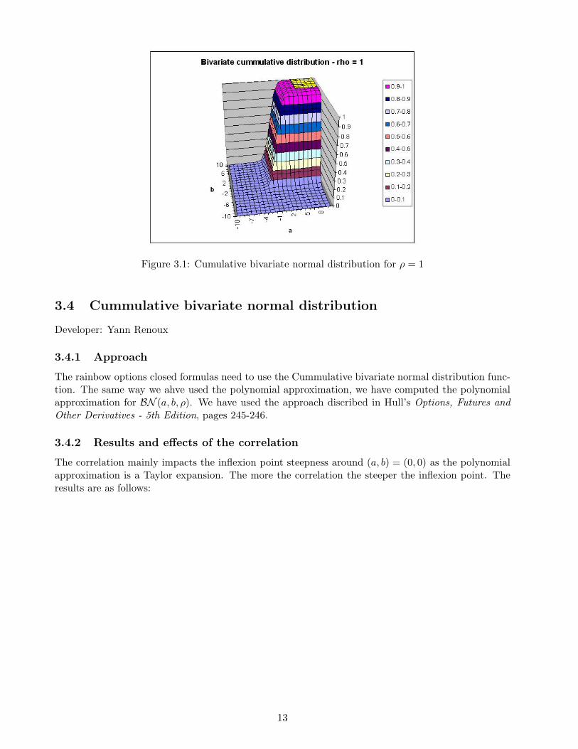
Figure 3.1: Cumulative bivariate normal distribution for ρ = 1

3.4 Cummulative bivariate normal distribution

Developer: Yann Renoux

3.4.1 Approach

The rainbow options closed formulas need to use the Cummulative bivariate normal distribution func-tion. The same way we ahve used the polynomial approximation, we have computed the polynomialapproximation for BN (a, b, ρ). We have used the approach discribed in Hull’s Options, Futures andOther Derivatives - 5th Edition, pages 245-246.

3.4.2 Results and effects of the correlation

The correlation mainly impacts the inflexion point steepness around (a, b) = (0, 0) as the polynomialapproximation is a Taylor expansion. The more the correlation the steeper the inflexion point. Theresults are as follows:

13

Figure 3.2: Cumulative bivariate normal distribution for ρ = 0

Figure 3.3: Cumulative bivariate normal distribution for ρ = −1

14

3.5 FileReader

Developer: Aloke Mukherjee

3.5.1 Approach

The FileReader class simplifies the task of working with structured data. Some examples of structureddata used in the project include swap and zero rates, option prices and credit spreads. We wanted tobe able to store this data in a simple comma-delimited text format so that it could be easily changedin a text editor. The FileReader bridges the gap between this human-readable format and the datastructures used in the project.

3.5.2 Implementation

The FileReader relies on the CSVParser class developed by Mayukh Bose to read comma-delimitedfiles. Reusing this class allowed us to avoid some of the headaches involved with parsing text. TheCSVParser class has a simple but powerful interface that pipes in data from the file and pipes it outas an appropriate data type. Some customization was required to allow the CSVParser to understandterreneuve-specific types like dates, credit spread types. Once the data has been transformed fromtext into valid data types, FileReader can construct the internal data structures which are requiredto instantiate classes such as credit curves or a volatility surface.

The other useful function of FileReader is discovering and caching the location of the commondata directory. The test routines use the cached value to locate their test data files.

15

Chapter 4

Part A: Black-Scholes and Monte Carlopricer

Developer: Simon LegerValidator: Aloke Mukherjee

4.1 Requirements

In this section, we write a model to price European options using the Black-Scholes formula and returnthe greeks associated to these options. We also write a monte carlo pricer to be able to check theprices for these options.

The formula for European options is depending on the type of the options (i.e. Call or Put) is :

C(S, T ) = SN (d1)−Ke−rTN (d2)

P (S, T ) = Ke−rTN (−d2)− SN (−d1)

where :

d1 =ln(S/K) + (r + σ2/2)T

σ√

T

d2 =ln(S/K) + (r − σ2/2)T

σ√

T

and the greeks are :

Calls Putsdelta N (d1) N (d1)− 1

gamma φ(d1)

Sσ√

(T )

vega Sφ(d1)sqrt(T )theta − Sφ(d1)σ

2sqrt(T ) − rKe−rTN (d2) − Sφ(d1)σ2sqrt(T ) + rKe−rTN (−d2)

rho KTe−rTN (d2) −KTe−rTN (−d2)

We then extend the previous model to provide the same results for the following strategies : -Long Call Spread - Long Straddle - Long Butterfly Spread

4.2 Design

We have two folders for this part : one named BlackScholes which contains the BlackScholes classwhich represents one european option and an OptionStrategy class which is basically a portfolio ofsuch options and provide important methods for them as an easy way to create some options inside.

16

4.3 Approach

To construct this, we see two important parts :

• One pricer using formula

• A generic pricer using Monte Carlo approach

One class (named Black-Scholes) computes the prices, implied vol and greek letters for a given typeof option (type is either Call or Put) and all this should be easily used through a nice OptionStrategyclass which is basically a portfolio of options. In this class you have the ability to add options bygiving their parameters or use friendly methods that construct for you some famous combinations, ashas been specified in the requirements.

Then we build a multiple-class based monte Carlo pricer which is driven by the MCEngine class.This pricer should be general enough to price various derivatives products as it generates a path forgiven dates, by taking into account the yield curve and the volatility surface built in this project,hence the possibility to price asian, look back options, etc.

4.4 Choices

We did not choose to use polymorphism for the black-Scholes and option strategy parts as both couldbe considered independent and use separately.

For the Monte Carlo pricer we used polymorphism in order for the user to be able to use differentrandom number generators and still have a robust interface Random class. The default numbergenerator is Sobol which is better than the default number generator of C++ and provides enoughnumbers to be generated if required.

In addition, the user has a drift class that can be modified easily to adopt other path generators.This one uses the extended Black-Scholes model by taking into account the yield curve and thevolatility surface so they are not considered constant through the path, which is useful for pathdependent options.

Then there is a GaussianProcess class which takes the lognormal process by adding the drift andthe random numbers generated and applying the corresponding volatility.

The Payoff class provides methods to take the path generated and the strike and returns the payoffaccording to the option specified.

There are four different sorts of number generators : the C++ default generator, the Park Millergenerator, the Mersenne Twister generator and also Sobol which is a quasi random generator. Hereis a comparison of precision for the different number generators : we try to price a european call, theexact price being 4.94387 :

300k 1M 10M 50MGenerator Price Time Price Time Price Time Price Time

RandC 4.96 2.156 4.935 7.172 4.9432 70.98 4.9461 355.62ParkMiller 4.987 1.968 4.962 6.532 4.9448 67.7 4.9446 324.09

MersenneTwister 4.936 1.984 4.949 6.547 4.9461 65.08 4.9435 325.73Sobol 4.94354 1.95 4.94372 6.42 4.94385 64.26 4.94387 319.95

As we can see, Sobol is way above the other generators for this kind of test. Obviously the goal ofa monte carlo number generator is to try to fit at best the interval [0,1] and for this a quasi numbergenerator is much better than any pseudo generator. The only point is that the numbers are lessrandom from a general point of view, since anyone can predict the next number, which is also possiblefor any algorithm but usually less easy. For 300,000 paths, we have the same precision with Sobol,

17

than with Mersenne Twister for 50 million paths ! And Mersenne Twister is known as the best pseudorandom number generators. To meet the same precisions as the other pseudo generators, the C++random number generator requires 5 times more paths and it is slower.

4.5 Unit tests

The unit test for this part was to build a market environment with a volatility surface and a yieldcurve and to compute the price of a european call and then to check the price with the monte carlopricer, after we checked some results with both online pricers and a pricer built in Excel with theclosed formula given by the Black-Scholes model.

4.6 Performance

We first implemented this pricer using double* instead of valarray<double> and the performance wasmuch better (almost two times faster). This is due to a fixed cost when you read a valarray due tothe cast type, but we chose to keep the version with valarray for a better integration with the rest ofthe code and to make it uniform and easier to read.

Another point could be to test other quasi random number generators to see if they are moreaccurate than Sobol, and also to make an interface for these random number generators to allow amulti dimensional generation for rainbow options for exemple. The implementation of Sobol algorithmis done with calibration up to 6 dimensions but we didn’t use it since the interface has been done forone dimension generation.

The last but not least point is that especially in banks, where most of computers have two proces-sors, it is possible to design the code so that it can use two threads to take advantage of the availableCPUs. An easier way that we tested was to create two executable files and run them on a same ma-chine (dual core Intel processor 2.8Ghz), but in this case one has to be careful about the initializationof the random number generators otherwise the price would be the same on the two threads. Afterthis, one just has to take the average of these prices. This would improve the performance by 80%,and maybe up to 250% with four threads on a machine with two processors with hyperthreading butwe couldn’t do this test since our dual core machine didn’t have hyperthreading.

4.7 Validation

The closed form formulas for European Calls and Puts as well as the Greeks Delta and Vega werecoded in Matlab (see BS.M in the data directory). These were then used to validate the C++ output.The Matlab version of Black-Scholes is quite simple to implement since there already exists functionsto calculate the cumulative normal distribution.

Another approach to validation was comparing with the results obtained by the use of the binomialtree. Since a binomial tree is less accurate than the closed forms for European options the value ofthis approach is debatable. Nonetheless it was observed that the binomial tree results were close tothe closed form and Monte Carlo solutions.

18

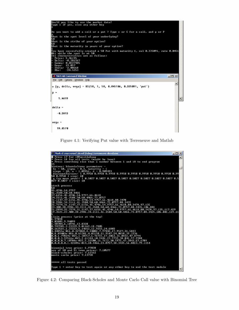
Figure 4.1: Verifying Put value with Terreneuve and Matlab

Figure 4.2: Comparing Black-Scholes and Monte Carlo Call value with Binomial Tree

19

Chapter 5

Part B: Yield Curve

Developer: Yann RenouxValidator: Joseph Perez

5.1 Requirements

All the formulas used in this project are based on risk-neutral valuation and non-arbitrage, with arisk free rate. Hence whatever the product we consider, we need to have a solid base class to handlethe needs of classes that define products. This object has to gather market data in the form of amarket yield curve and provide the basic methods expected. Such methods go from getting the spotzero coupon – ZC – rate for a certain maturity, the discount factor to present value future cash-flowsor forward rates to evaluate such future flows. But these methods can also include different interestcomposition, such as annual or continuous.

5.1.1 Other methods we added for risk management purposes

In addition to the basic methods required, we have added a shift and a rotation to model the 2 firstknown factors of the Principal Component analysis on the term structure of a yield curve:

This will be very useful in term of risk management, as we know that all the rates bear a correlationand the term structure is very unlikely to revert from one day to the other.

For instance, a yield curve is a set of data points with ascending maturities, related to some fixed-income product that provides a yield. In practice, the short end of the curve comes from the ZCB’s,and the rest is from the swap market. As those 2 evolve in a different space, the object needs to rotatethe space of swaps into ZC rates.

We mentioned the methods we want the yield curve to be able to perform, but not what it willuse as base data. We have decided to store the term structure from the market curve, which is madeof zero coupon rates for short maturities – 0.25, 0.5 and 1 year for the US market – and swap rates –from 2 to 10, 15, 20 and 30 years in the same market. As these rates do not come from the same sort

Figure 5.1: 3 first axis of the PCA (95% of the variance): Shift, Rotation and Curvature

20

of product, they do not belong in the same space, hence a transformation needs to be done to havethem in comparable values: the class must be able to do the rotation transparently.

5.1.2 From swap rates to ZC rates

Consider a swap with notional N such that:

• the floating leg delivers m flows at dates Tj for j = 1...m

• the fix leg with rate C delivers n flows at dates Tki for i = 1...n, k being the ratio between theannual frequency of payment of the floating versus the fix leg, so that kn = m.

The so-called zero-coupons method provides a way to evaluate this vanilla swap, being equal tothat of:

• a fixed coupon bond with same maturity and notional

• minus the swap notional (a swap does not exchange principal).

Hence, defining B(t, Tki) the value at t of a ZC paying 1 dollar at Tki, we can write:

SWAPt = N

(n∑

i=1

CB(t, Tki) + B(t, Tm)

)−N

where at any given date, the fix rate C is the par swap rate, giving the NPV equal to zero.Thus at t, each swap rate s(t, .) verifies:

1 =m−1∑i=1

s(t, m)(1 + R(t, i))i

+1 + s(t, m)

(1 + R(t, m))m

Writing them up for all known maturities between 1 and m, we get matricially:

1 + s(t, 1) 0 0 0

s(t, 2) 1 + s(t, 2) 0. . .

......

. . . . . . 0s(t, m− 1) s(t, m− 1) 1 + s(t, m− 1) 0

s(t, m) · · · · · · s(t, m) 1 + s(t, m)

1(1+R(t,1))1

...

1(1+R(t,m))m

=

1

...

1

that is to say:

A(t)

1(1+R(t,m))1

...

1(1+R(t,m))m

=

1

...

1

hence

1(1+R(t,1))1

...

1(1+R(t,m))m

= A(t)−1

1

...

1

Hence if we have all the intermediary points, we can just back out the ZC rates while solving an

easy triangular system. We will come back to the assumptions we made here later.

21

5.2 Design

5.2.1 Approach

Prior to studying what a yield curve is, a simplier object should be defined, the yield point. Its 4members are :

• a type (Cash or Swap - but can be extended to other instruments),

• a rate,

• a maturity in years, and

• a Daycount convention (defaulted to Actual/360, the most common convention for USD Liborswap rates).

Note that the maturity is not a date, as commonly people talk about the 5 years swap rate or the1 year ZC rate. The yield curve will be able to transform one into the other so that the user can useboth.

A yield curve is then a valarray of yield points, but can be assigned a flat rate in anotehr construc-tor. At the construction, we need to make sure that the transformation is being made according tothe method exposed earlier, so that the user can build a yield curve with several types of rates and beable to back out the tools without adding any line of code. In addition to that, the yield curve objectalso has a name field, so that the user can define a ”USD Libor Curve” or a ”EUR Libor Curve”.

5.2.2 Choices

As we said earlier, to get the ZC rates from the swap rates, we need to solve a triangular system. The1 year swap rate is the 1 year zero coupon rate (write the formula...), but then it depends on what isthe type of swap rate we are talking about. Say we have market quotes on semi annual swap rates,then we would need the 1.5 year swap rate to back out the 1.5 year ZC rate as we know the 1 year one.Here the choice was made to consider annual swap rates – as in the Bloomberg quotes file provided,as well as a linear interpolation when needed. For instance, we have here solved the 1-10 years issueas all maturities there follow each other, but what for the rest ? Well the 12 years swap rate is takenas the weighted average of the nearest higher and lower rate known, here 15 and 10 years. We did notcode splines interpolation method, as we thought that was not the main emergency in the class. As aresult, we face a little bump on the reconstruction after the 10 year ZC rate due to this approximation:

We supposed that the user provides rates non ordered by maturity or type, then it does the sortingby itself. All the same if the user does not enter all rates, the swap to ZC private method does allwhat is needed to handle it.

5.2.3 Methods

On top of the necessay methods already mentionned (discount factor, forward rate, sorting, invertingswap to ZC, shift or rotate the curve, etc.), the yield curve has an output operator ”<<” for easychecking, as well as a comparison one ”==”.

5.2.4 Unit tests

We used the file we provided from BBG (US Yield Curve ”IYC”, October, 5th, 2005). We computedzero coupons and output them as we saw earlier, computed some spot rates, discount factors, forwardrates for different maturities in years or date, and changed the conventions. We have compared themto the calculus by hand in Excel, to make sure the results were coherent, as this class needs to beaccurate for all the forthcoming ones.

22

Figure 5.2: ZC curve reconstruction from annual swap rates from 1-10 years, 15, 20 and 30 years.

Figure 5.3: Bloomberg YC Data for USA

23

Figure 5.4: Graph of the continuously compounded discount factors up to 30 years

We can note that the decreasing effect of the discount factor seems to be appropriate. See section4. of the module to visualize the tests ran, as well as the validation part.

Figure 5.5: Graph of the forward rates starting in 6 months

On the forward rate graph, there is a break at (6m,6m) which corresponds to the change fromZC to swap rates, indeed the interpolation method has a huge impact on the forward rates. Seehttp://www.riskworx.com/insights/interpolation/interpolation.htm for more explanation. We concludethat for our purpose, the forward curve is satisfactory, and as mentionned, could be improved byimproving the interpolation method.

To finish, we tested the several methods, spot, discount factor, forward rate and compared tothe calculus we should have, just by using the yield curve and calculating the expected prices. Theywere all in line – see the mainyieldcurve program in the test directory for more details. Results in in

24

data/rates.xls

5.2.5 Performance

We have mentionned various assumptions, and their addition would increase the computation time.For instance, the flexibility of swaps frequency, or the splines interpolation.

But as is, aside of the valarray that might not be ”the” efficient structure for a too small amountof data, some methods or storage could be improved. As an example, all the getSwapRates - maybewe could store them separately at the construction and avoid needing to find them, etc. Also, thegetSequentSwapRates, used to the first part of the curve 1Y-10Y, is used only to be able to knowwhether or not to interpolate. It might be redundant if the list of swaps we get for the matrix invertionwas better seen.

5.3 Validation

5.3.1 Approach

A way to validate the construction of a yield curve was to compute prices of zero coupon bond ofshort maturity and the swap rates with a yieldCurve object and compare them to the input we gaveto construct it. They matched. The other validation method was to use the yield curve in every othersection. As with the other objects (bond, montecarlo...) we got good results it means that the yieldcurve was well defined.

25

Chapter 6

Part C: Asset

Developer: Yann RenouxValidator: Joseph Perez

6.1 Requirements

This is an underlying asset class. It has a currency, a spot price level and a dividend schedule or afixed dividend rate. It also possesses a yield curve, supposingly in his currency of denomination, whichpurpose is to discount future flows. We have made the choice not to use it as a member for the otherclasses, but it bears all the necessary information. It could be used as to provide a dividend growingrate for Black Scholes object for example.

Hence the choice has been made not to use an asset with a volatility surface that would simulateitself forward prices, as indeed it would be a single simulated price, and in expectation, the volatilitydoes not enter into account.

The only purpose of this object is to be able to be added in the portfolio to hedge options on thebook.

6.2 Design

Obviously a stock is a delta one security, the interesting thing is the benefit of carry with the dividendsversus its cost of carry against the money we would get while depositing the money at the currentmarket rate.

The other thing is that usually, with no inside information on the company, one cannot know forsure the future dividends that will be paid. Thus we decided to add the fixed dividend rate, whichin practise would be an econometrically estimated parameter, but a very commonly used input inpricing, such as in Black-Scholes for instance.

The well-known formula for pricing a stock with dividends is:

Pt =∞∑i=1

Dividendt+i ×DiscountFactor(t, t + i)

Hence the forward price:

F (t, T ) = PT =∞∑i=1

DividendT+i ×DiscountFactor(t, T + i)

In practise it would be the current price minus the known future dividends up to the date T . Thisentails and reflects the drop in price that a stock sustains when a dividend is paid: it theoretically

26

Figure 6.1: Asset forward price - comparison of a fixed continuous rate versus a dividend schedule

decreases its current price by the exact amount that has been paid. On the contrary, with a fixeddividend rate q, the forward price is F (t, T ) = Pte

−q(T−t). The following graph reflects this noticedfact.

The continuous rate has been taken equal to 7.5%, while for the purpose of demonstration, thedividend schedule in the other case is up to 10 years, with 5% the even years, and 10% the odd years.The first noticeable fact is the sudden drop when the dividend is paid. This is not on an accrual basisas the bonds! On the other hand, the graph goes beyond the 10 years, and we remark that by thenthe forward price of the dividend scheduled asset remains constant, which is in agreement with theformula. Last note that the apparently increasing forward price is not the reality, it is just due tosmoothing in Excel graph – look at the output file produced by the test menu to check it.

6.3 Approach

The dividend schedule is a valarray of flowSchedule, a class with a date, an amount in percent, and abusiness day convention for the payment date. Indeed, if the payment date does not fall on a workingday, the accrued interest calculation can differ depending on the convention.

An asset then has the mentionned members, should the user specify in the constructor the type ofdividend, fix rate or scheduled. All the methods check this before pricing.

6.4 Methods

The forward price is using the formulas mentionned above, and the class has a getDelta function sothat the portfolio class can know that holding an asset is delta one.

The getPrice method has been made virtual so that if later we want to inherit from this, we cando it.

6.5 Unit tests

We have tested several dividend rates, and schedules, checking that the forward drops on the paymentdate by the expected amount. The output file for the 10 year dividends illustrates well what we did.

27

6.6 Performance

This class being rather simple, nothing huge can be done to make it quicker. And if so, this was notat all the most important object to improve. See the mainasset in the test directory for more details.

6.7 Validation

No particular validation test were needed for this simple class, we just had to check that code had nobug and formula for forward price was correct.

28

Chapter 7

Part E: Implied volatility surface

Developer: Joseph PerezValidator: Simon Leger

7.1 Requirements

Giving a matrix of call and put prices for a range of maturities and strikes and a yield curve allows usto invert the Black-Scholes formula for each price to get the implied volatility. In plotting the matrixof implied volatilites we create an implied volatility surface.

According to Black-Scholes option pricing model, the volatility for calls and puts for the samematurity should have the same volatility of the stock price and the implied volatility surface shouldbe a term structure. However market prices indicate that volatilities depend on strikes level. Theimplied volatility surface of market prices looks like a smile.

7.2 Design

We build an implied volatility surface for an underlying from its price, a yield curve and a table ofstandard european call/put prices for different maturities and different strikes.

Black-Scholes’ model makes it possible to price a call or a put with closed form solution if weconsider constant volatility and constant interest rate. But the classical option pricing formulas canbe inverted and we can compute what is commonly call the implied volatility if we know the price.

According to Black-Scholes option pricing model, the volatility for calls and puts for the samematurity should have the same volatility of the stock price and the implied volatility surface shouldbe a term structure. However market prices indicate that volatilities depend on strikes level. Theimplied volatility surface shape can be different depending on the underlying. Smile, smirk or sneerare kinds of name we give to caracterize those shapes. For equity index options markets, it is more ofa skewed curve. This has motivated the name ”volatility skew”.

European options on stock are often liquid and option prices are given by the market. We use forthe price the midpoint of Bid/Ask.

7.3 Approach

7.4 Choices

Once our price inverted we have a range of implied volatilites for different levels of strike and differentmaturities. Then we can get the implied volatity (or variance) for a given strike and a given maturity

29

Figure 7.1: Volatility surface of S&P500

using a quadratic interpolation. As the implied volatility surface is rather smooth a local 2D quadraticinterpolation gives us good approximation.

7.5 Methods

For each maturity and each strike for which we have the price of a call or a put, we create a BlackSc-holes object. The constructor of BlackScholes class inverts Black-Scholes formula using the recursiveNewton-Raphson algorithm in order to get the implied volatility.

Once the implied volatility surface is set we can compute the implied volatility (or variance) forany maturity and any strike. To do this we use the 2D-quadratic interpolator. As the surface is rathersmooth and looks like a parabol, a quadratic interpolation gives us good approximation.

The class includs a method to compute a forward volatility. Assuming we built our impliedvolatility surface at time t and we want to know what would look like the volatility at time T2 seenat T1 for a strike K. We use the following formula

σ2T1,T2

(K) =σ2

T2(K)(T2 − t)− σ2

T1(K)(T1 − t)

T2 − T1

7.6 Unit tests

We build the implied volatility surface for the S&P500 from call and put prices of July 2004. Theshape we get is as expected, it is a ”skewed surface”.

7.7 Performance

The Vega of call/put is always positive option prices are increasing function of the volatility that’s whyNewton-Raphson algorithm is accurate in this case. By default inversion of Blacks Scholes formulareturn the computed volatility after 100 iterations. In practice the volatility converges quickly, only10 iterations are necessary. So we could either set the number of iterations to be 20 or to compareafter each iteration the difference |σn+1 − σn| and exit the loop as it is inferior to a level ε.

30

Figure 7.2: Linear Volatility surface

7.8 Validation

7.8.1 Approach

To test this class, whose accuracy is very important for the rest of the project, we ran two tests.First we instanciated an object of the volsurface using the flat volatility constructor and we checkedthat every point was giving the same and correct volatility and we also checked the values of forwardvolatilities in an Excel spreadsheet by replicating the formula.

Then we created a bench of strikes and dates in an Excel spreadsheet and by choosing a volatilityfor these points, just arbitrary. We compute the black scholes price for each of these options andwe load these prices, dates and strikes into our c++ project and construct the yieldcurve with them.After this, we decide to get some volatility from this object for some strikes and matuirties and wecheck if they give exactly the same result than for the inputs and nice enough results for other points.Then we simply plot the volatility surface in a two dimensional chart to check its shape.

Here is the table for these volatilities given the strikes and maturities transformed in years :maturity 2395.95 2545.69 2695.44 2770.31 2845.19 2920.06 2994.93 3069.81 3144.68 3294.43

0.1697467 0.2 0.19 0.18 0.17 0.16 0.15 0.14 0.13 0.12 0.110.6680356 0.22 0.21 0.2 0.19 0.18 0.17 0.16 0.15 0.14 0.131.4154689 0.24 0.23 0.22 0.21 0.2 0.19 0.18 0.17 0.16 0.152.4312115 0.26 0.25 0.24 0.23 0.22 0.21 0.2 0.19 0.18 0.174.4243669 0.28 0.27 0.26 0.25 0.24 0.23 0.22 0.21 0.2 0.197.4332649 0.3 0.29 0.28 0.27 0.26 0.25 0.24 0.23 0.22 0.21

As one can see we constructed a linear volsurface, increasing with maturity and decreasing with strike,and here is the plot of this surface :

31

Chapter 8

Part F: Credit Curve

Developer: Aloke MukherjeeValidator: Yann Renoux

8.1 Requirements

A credit curve is similar to a yield curve in that it can be used to calculate discount factors andthus present or future values of a risky security. The key difference is that there is a spread at eachmaturity between the credit curve and the yield curve corresponding to the additional return requiredfor taking on the added risk.

Credit curves are associated with the issuer’s creditworthiness. There is always a probability thatthe issuer will default and thus be unable to meet their debt obligations. A survival probabilityquantifies the probability at any given time that the issuer will ”survive” to meet these obligations.Survival probability declines with time and declines faster for less credit-worthy issuers.

We calculate implied probabilities from credit default swap spreads. In a credit swap the buyer ofprotection pays the spread periodically and the seller pays in the event of a default. These two legsmust have equal present values. The assumption underlying this model is that the spread on a riskyasset vs. a non-risky asset is entirely compensation for the possibility of default. The CreditCurveclass models the modified yield curve as well as the issuer’s survival probability, hazard rate andrecovery rate.

8.2 Design

All of the discounting functionality can be reused from the YieldCurve object. The CreditCurve objectmust also maintain a collection of spread points.

The more interesting part of the implementation was bootstrapping the default probabilities. Wedecided to implement the calculation recursively. We define the following terms:

qn - default intensity. This is the probability of default in period n conditional on no earlier default.Qn - default probability. This is the probability of default in period n as seen from time 0.Sn - survival probability. This is the chance of survival to time n.Cn - cumulative default probability. This is the chance of default before time n. It is the comple-

ment of Sn. This value is called Qn in Professor Laud’s notes.Fn - fees associated with one leg of a credit default swap. Both legs are assumed equal to this

value so the quantity can be computed either from the perspective of the buyer or seller of protection.B(0, tn) - discount factor. The value of one dollar received at time tn.sn - spread. The credit spread over the riskfree rate at time n.

32

R - recovery rate. The proportion of face value recovered in the event of default. It is usuallyassumed to be 40%.

The following relationships hold for these quantities:

q0 = 0, q1 = Q1

Q2 = (1− q1)(q2) ⇒ Qn = (n−1∏i=1

(1− qi))qn

Sn = 1−n∑

i=1

Qi =n∏

i=1

(1− qi)

Cn = 1− Sn =n∑

i=1

Qn

Generalizing from the risk-neutral argument of equality between swap legs at each default time wecan write down the following recursive formula for qn in terms of fees Fn, survival probabilities Sn,spreads sn, recovery rate R and appropriate discount factors:

qn =Fn−1( sn

sn−1− 1) + B(0, tn)snSn−1

B(0, tn)Sn−1(1−R + sn), q0 = 0(probability of default at time 0 is 0%)

Sn = Sn−1(1− qn), S0 = 1(probability of survival at time 0 is 100%)

Fn = Fn−1 ×sn

sn−1+ B(0, tn)snSn−1(1− qn)

F0 = 0(no fees at time 0)

By implementing recursive methods for default probability, survival probability and fees we cancalculate default intensities at discrete time intervals. Notice that all the above is considered in thediscrete time setting for simplicity of implementation and because of the discrete nature of the spreaddata.

8.3 Choices

There are three choices with respect to reuse of the YieldCurve class. CreditCurve can inherit fromYieldCurve, YieldCurve and CreditCurve could both inherit from some common class or CreditCurvecould contain a YieldCurve.

The first two have the benefit of allowing polymorphism - e.g. a function designed to take a Yield-Curve object and use it for discounting can also take a CreditCurve object. This would not be possiblein the third case unless there were some method of CreditCurve which returned a YieldCurve. This iscumbersome. Of the two polymorphic approaches the first has the benefit of simplicity and intuitive-ness: namely there is no object more basic than a YieldCurve in finance and secondly the CreditCurveis a type of YieldCurve rather than a type of some other more basic object. Our implementation takesthe first approach.

In calculating default probabilities we decided to throw out the .5 year spread since keeping itrequires having a special case. Instead we standardize the calculation on 1 year intervals - i.e. weassume that defaults happen at the 1/2 year mark. Another justification for this is that looking at the

33

Figure 8.1: Bloomberg CDS data for AIG

sample data we received for AIG from Bloomberg, it appears that the .5 year spread is interpolated(equal to 1 year spread).

We also decided to internally interpolate spreads at 1 year granularity rather than working withdiscontinuities in the spread data. Hull suggests one approach for calculating default probabilities onan interval where there is no spread data: assume a constant unconditional default probability in eachperiod. Since the calculations implemented here work with conditional default probabilities it is easierto assume a spread and leave the calculation as it is. From the rough relationship

h =s

(1−R)

we know that spreads are proportional to conditional default probabilities. So interpolating spreads islike assuming a constant default probability in the interval. The approach of using a constant defaultintensity is suggested in section 21.3 of OFOD (6th edition). For another supporting argument forthis approach see http://www.fincad.com/newsletter.asp?i=1140&a=1800 which suggests interpolat-ing CDS spreads as an improvement vs. constant ”default density” (a.k.a. unconditional defaultprobabilities).

The risky discount factor was calculated by multiplying the underlying riskfree discount factorby the discrete time survival probability up to that time rather than using a continuous hazard-ratefunction. In the class notes we have RF = DF × (1−Q(T )). Q(T ) is cumulative default probability(in Professor Laud’s notes, here we denote it Cn) so it is the complement of S(T ), the cumulativesurvival probability.

In discrete time we have the identity: (Sn−Sn+1)Sn

= qn. qn is a discrete time version of hazard rate.In the limit this leads to the expression S(t) = exp(−

∫ t0 h(t)dt).

The risky discount factor is a ”discounted” discount factor - the discounting applied is the survivalprobability. In continuous time we can use the expression above but since we have calculated everythingto this point in discrete time and we have an explicit expression for the survival probability we usethis as the discount factor rather than the continuous time expression above.

34

Figure 8.2: Credit spreads

Figure 8.3: qn - hazard rate or default intensity

8.4 Unit tests

The recursive algorithm was first implemented in Matlab. The M-files can be found in the datadirectory:

defprob.m, survprob.m, fees.m

Using Matlab some of the results in section 21 of OFOD were successfully reproduced. When imple-mented in C++ the results were verified against the Matlab output as well as the example in OFOD.Another source of verification was the reuse of the credit curve class in implementing the risky bond.

Additionally the given data for AIG was encoded in a file and used to instantiate a CreditCurve.The data was gathered using CreditCurve’s appropriate methods and plotted here and on the followingpages. The cumulative default probability curve comes quite close to the Bloomberg curve.

35

Figure 8.4: Comparison between calculated and values from Bloomberg

Figure 8.5: Survival probability

36

Figure 8.6: The risky discount factor

8.5 Performance

Recursion can be time-consuming resulting in many nested calls. One approach to improving perfor-mance is to cache intermediate results. Caching was implemented and makes the performance O(n)for the first call (assuming you are calculating default probabilities from earlier to later periods). Onceall values are cached, results are immediate. Overhead for the first call could be further reduced if thevalues were cached at construction.

The best candidate for performance improvement in the CreditCurve class is probably the methodused to construct the curve. The spreads are all converted to relative spreads and then used toconstruct a new yield curve. Then the spotrates of the underlying curve and the ”spread curve” aresummed to instantiate a combined curve. This procedure is a bit overly time and memory consumingand could be optimized.

8.6 Validation

8.6.1 Approach

We applied the algorithm present in Pr. Laud lecture notes. Define

• A spread sprdT is paid annually constantly to protect for the default during T years.

• qi = q(i− 1, i) is the conditional probability of default in period i. q0 = 1

• Q(i) is the cumulative probability such as Q(0) = 0 and Q(i + 1) = Q(i) + qi+1[1−Q(i)]

To compute we note that the Present Value of the fees on the whole life should equal the lossoccurred in case of default, all been on the point of view of the seller. If we call B(0, j) the risk freediscount factor up to year j and R the recovery rate:

37

E(PV Fees, T ) = sprdT ×T∑

i=1

B(0, i)i∏

j=1

(1− qj)

E(Loss, T ) = (1−R)×

T∑i=1

qiB(0, i)i−1∏j=1

(1− qj)

The first conditional probability is easy to compute, and we used Excel’s ”Goal Seek” to find

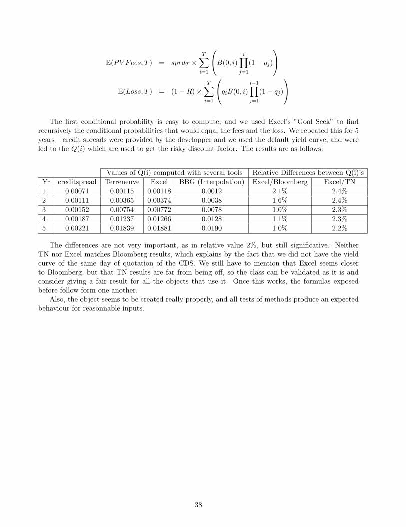
recursively the conditional probabilities that would equal the fees and the loss. We repeated this for 5years – credit spreads were provided by the developper and we used the default yield curve, and wereled to the Q(i) which are used to get the risky discount factor. The results are as follows:

Values of Q(i) computed with several tools Relative Differences between Q(i)’sYr creditspread Terreneuve Excel BBG (Interpolation) Excel/Bloomberg Excel/TN1 0.00071 0.00115 0.00118 0.0012 2.1% 2.4%2 0.00111 0.00365 0.00374 0.0038 1.6% 2.4%3 0.00152 0.00754 0.00772 0.0078 1.0% 2.3%4 0.00187 0.01237 0.01266 0.0128 1.1% 2.3%5 0.00221 0.01839 0.01881 0.0190 1.0% 2.2%

The differences are not very important, as in relative value 2%, but still significative. NeitherTN nor Excel matches Bloomberg results, which explains by the fact that we did not have the yieldcurve of the same day of quotation of the CDS. We still have to mention that Excel seems closerto Bloomberg, but that TN results are far from being off, so the class can be validated as it is andconsider giving a fair result for all the objects that use it. Once this works, the formulas exposedbefore follow form one another.

Also, the object seems to be created really properly, and all tests of methods produce an expectedbehaviour for reasonnable inputs.

38

Figure 8.7: Cumulative default probabilities – BBG vs TN vs Validation

39

Chapter 9

Part D: IR Vanilla Swap

Developer: Simon LegerValidator: Yann Renoux

9.1 Requirements

In this section, we develop an object that represents the behavior of a vanilla interest rate swap.An interest rate swap is a contract where two parties exchange cash derived from the interest on

a notional principal. Typically, one side agrees to pay the other a fixed interest rate and receives afloating rate.

We first write an object that represents the characteristics of a cash flow object, which takes ayield curve and a swap leg and computes cash flows to maturity. For this we developed a swap legobject which is just one side of the contract and stored the required information depending on the leg.We then wrote a method to compute the fair value of a swap leg which is the discounted value of itscash flows.

We then extended our object to include amortizing swaps, where the notional declines accordingto a prescribed schedule.

9.2 Design

To construct this, we started by the swap leg object which takes some dates and notionals as vectorsor can also take a start date, an end date and a frequency and computes the payment dates and alsoa notional and a constant amortizing value for it and compute the different notionals at each date,according to a certain business day convention.

Then, the CashFlow object takes a swap leg and either a fixed rate or a yield curve to compute thecash flows at each time. We also have a method which takes a yield curve used for discount factorsand computes the fair value of the swap.

9.3 Approach

9.4 Choices

The choices for this part are very limited as everything is almost described in the project and theliberty is then very reduced. We decided to follow our main objectives in this project, that is the useof valarray and we tried to write the objects as generic as possible to allow them to be modified orcomplexified easily later.

40

9.5 Unit tests

The value of a swap paying X% fixed and receiving a floating rate, with a yieldcurve flat at X% hasbeen calculated and the price returned was 0.

9.6 Validation

9.6.1 Approach

Valuating a vanilla swap is actuarial science, so as long as we have the same yield curve as an input,we should be able to match the results exactly.

We have done the tests in Excel using the default yield curve hence, as the yield curve has beenvalidated, we are sure of the inputs and now have to check the calculation. It has been done for afixed notional of 1, 000, 000 but the class is designed so as to take any set of indexed notionals (hasbeen checked). We have modelled a 5Y annual swap and a 4Y semi annual swap both paying floatingversus receiving fixed. The results match exactly except for the floating leg of the semi annual swap,but even after checking that we had the same compounding method for the discount factors and theforward rates (the floating leg is a set of forward rates) and the numbers were excatly in line in C++versus Excel, we have not been able to detect what the issue was. Note that it is 800 on a notional of1, 000, 000 though.

It might be at first approximation the fact that the floating leg computing each and every floatingrate for each period, their multiplication populates errors as linear interpolation of the yield curvedoes not fit properly the yield curve.

5Y Annual Swap @ 4.71% 4Y Semi-Annual Swap @ 4.641%TN Excel Diff TN Excel Diff

Fixed 205,345 205,345 - 167,481 167,481 -Float 204,294 204,294 - 167,329 168,129 (800)Value 1,051 1,051 - 152 (648) (800)

9.6.2 Pitfalls

No major pitfall was found. The objexct behaves properly, the only thing being these slight differenceswith non annual swaps and with exactly the same forward rates and discount factors. Results indata/IRSwapValidYann.xls

41

Chapter 10

Part H: Treasury Bonds/Risky Bonds

Developer: Joseph PerezValidator: Aloke Mukherjee

10.1 Requirements

In this section we design an object that take into account the characteristic of a bond (either a treasurybond or a risky bond) mainly in order to price it.

Usually on the contract of a bond are specified the maturity, the date of the first coupon, the dateof issue, the annual value of coupons, their frequency, the faceamount and the daycount convention.Those are information are required to create a bond object.

10.2 Design

Treasury bond and risky bond are similar except that to be priced we use a yield curve for the T-bondand a credit curve for the risky bond. As those bonds are closely tied with those curves we decided toincorporate them into the constructor. We designed one class for T-bonds and another one for riskybonds. Both inherits from a generic class bond.

10.3 Choices

As a bond price is a decreasing function of its yield to maturity, We find the yield to maturity for agiven price with the recursive Newton-Raphson algorithm.

10.4 Methods

We implemented several methods :

• getCashflow returns an array of cash flows with their dates

• quotedPrice which is the present value of the cash flows

• fairvalue, the sum of the quotedPrice and the interest accrual

• yieldToMaturity, duration and convexity

At time ti we have the cash flow CFi = facevalue ∗ coupon/frequency and if ti is the time of the lastcoupon CFi = coupon/frequency+facevalue, the discount factor between 0 and ti is DFi is given by

42

Figure 10.1: bond prices for different maturities

the yield/curve. Let t′ be the time between the reception of the last coupon (if there had one else thedate of issue) and today and t′′ be the date of the reception of the next coupon and the time betweenthe reception of the last coupon (if there had one else the date of issue). Let also y be the yield tomaturity.

quotedPrice =∑

i

CFi ∗DFi

fairvalue = quotedPrice + facevalue ∗ coupon ∗ t′/t′′

duration =∑

i CFie−ytiti

fairvalue

convexity =∑

i CFie−ytit2i

fairvalue

10.5 Unit tests

The chart had been drawn with bonds having the following specificities

bond treasury bondcoupon 4.5%

daycount ACT/365frequence semianual

faceamount 100

The values we get are in accord with the Treasury bond provided. We can’t claim we found exactlythe same price because we didn’t have the yield curve at that time.

10.6 Performance

Most of methods implies simple computations so it would be difficult to improve the efficiency of thisclass. We use Newton-Raphson algorithm, the comment on this algorithm in the section VolatilitySurface holds.

43

10.7 Validation

10.7.1 Approach

We used inputs of table 5.7 ’Calculation of duration’ of Options, Futures and Other derivatives (fourthed.) by John Hull to compare our duration to theirs. Both duration matched.

44

Chapter 11

Part I: Rainbow Options

Developer: Yann RenouxValidator: Simon Leger

11.1 Requirements

In this section, we wrote an object that represents the characteristics and behavior of rainbow optionswith an eye towards extending to more than 2 assets and a variety of pay off functions. as such, ourobject was supposed to report for 2 assets:

• S1 and S2 are prices of asset 1 and asset 2 at exercise

• W1 and W2 are the respective weights

• K is the strike

• M is a multiplier 1=CALL, -1=put

• Spread Option max {M * (W1*S1 W2*S2-K), 0} - Type SpreadOptionMax in the class

• 2-asset basket max {M * (W1*S1 + W2*S2-K), 0} - Type AssetsBasketMax in the class

• Best Of 2 assets and cash max {W1*S1, W2*S2, K} - Type BestOf2AssetsCash in the class

• Worst Of 2 assets and cash min {W1*S1, W2*S2, K} - Type WorstOf2AssetsCash in the class

• Maximum Of 2 Assets max {M * (max[W1*S1 , W2*S2]-K), 0} - Type Max2AssetsCall /Max2AssetsPut in the class

• Minimum Of 2 Assets max {M * (min[W1*S1 , W2*S2]-K), 0} - Type Min2AssetsCall /Min2AssetsPut in the class

• We also added the BetterOf2Assets / WorseOf2Assets, which is basically the BestOf2AssetsCash/ WorstOf2AssetsCash with a strike equal to 0.

As we really had an eye towards more than 2 assets, we do not take a single correlation asparameter, rather a correlation matrix on which we perform Cholesky decomposition to correlate thenormal samples (see next section). Of course a default constructor with a ”Real” as correlation hasbeen implemented. The object uses any set of weights – they need not be equal to 1 in sum, as theoption can provide leverage or low exposition, a volatility surface for each stock and a single yieldcurve. Indeed we have made the choice not to consider for now quanto options, so each stock havingthe same currency, there need not be more than one yield curve.

45

This framework activelly uses the Monte Carlo Engine, but we discovered some interesting thingsas for which random number generator to use, and how to use it efficiently.

You will write an object allows you to simulate stock prices in the future. This object shouldtake a list of underlying stock assets, volatility surfaces and correlation matrices and be able to getsimulated prices for each stock at any time T. Using the two assets provided, implement the rainbowoptions described above. Write methods to Compute the fair market value of the option. Computepartial delta, partial gamma and partial vega with respect to the two assets. Compute a measure forCorrelation Risk for any pair of assets i.e. a change in price of the option for a change in correlationbetween the 2 assets. Validate your model using closed form solutions wherever applicable. As partof your report, describe your test cases, results and a graph the difference between prices and greeksobtained using closed form and prices obtained using simulation.

11.2 Design

We have already explained the payoff types we implemented, and to check our prices we used theclosed forms when it was applicable. Rubinstein wrote in 1991 and 1995 in ”Somewhere Over theRainbow” and ”Return to Oz” that spread options, basket options and dual-strike options do nothave a closed form. Also, for the Worst Of 2 Asset plus Cash we were not able to derive a closedform, but there should be one. As for the other types of rainbow options, we refered to the web-sitehttp://www.global-derivatives.com/options/rainbow-options.php to get them. For these the weightsare taken equal to 1 for each stock, and for the Best Of Cash/Worst Of Cash/Better/Worse, themultiplier is equal to 1. The closed forms use the following variables with usual notations:

σA =√

σ21 + σ2

2 − 2ρσ1σ2

ρ1 =ρσ2 − σ1

σA

ρ2 =ρσ1 − σ2

σA

d1 =ln(

S1K

)+ (r − q1 + 1

2σ21)T

σ1

√T

d2 =ln(

S2K

)+ (r − q2 + 1

2σ21)T

σ2

√T

d3 =ln(

S1S2

)+ (q2 − q1 + 1

2σ2A)T

σA

√T

d4 =ln(

S2S1

)+ (q1 − q2 + 1

2σ2A)T

σA

√T

Now if we denote by N the cumulative normal distribution and BN the cummulative bivariatenormal distribution, both approximated using Hull’s coefficients (see Chapter ”Common”), we define:

A = S1e−q1T [N (d3)− BN (−d1, d3, ρ1)]

B = S2e−q2T [N (d4)− BN (−d2, d4, ρ2)]

B = Ke−rTBN (−d1 + σ1

√T ,−d2 + σ2

√T , ρ)

With these inputs we can then get the prices with closed forms:

46

Type of Rainbow Closed Form price(1) Best of 2 Assets Plus Cash A + B + C(2) Maximum of 2 Assets Call (1)−Ke−rT

(3) Better of 2 Assets A + B + C (Where K = 0)(4) Maximum of 2 Assets Put (2)− (3) + Ke−rT

(5) Minimum of 2 Assets Call EuroBSCall(S1)+EuroBSCall(S2)− (2)(6) Worse of 2 assets EuroBSCall(S1)+EuroBSCall(S2)− (3)(7) Minimum of 2 Assets Put EuroBSPut(S1)+EuroBSPut(S2)− (4)

From there we understand that we can also check our formulas by synthetizing on with someothers and compare. For example, we have priced all of these for several strikes, spots, volatilities andcorrelations (see test on rainbow) and substracting (2) from (1) gives at Ke−rT at the 5th decimalfor closed form and the second for Monte Carlo. The other combinationes were tested too and arein agreement. See the Monte Carlo later in this chapter to see how we made sure our tests wereconsistent.

To generate two correlated brownian motions (X1, X2), we have to sample 2 normal distributions(N1, N2) and do the following:

X1 = N1 (11.2.1)

X2 = ρN1 +√

1− ρ2N2 (11.2.2)

In higher dimension, we use the Cholesky decomposition for a correlation matrix Σ for n brownianmotions, we write

Σ = UT U

where U is a lower triangular matrix. ThenX1

...

Xn

= U

N1

...

Nn

The 2 dimension formula is a special case of the Cholesky decomposition with(

1 ρρ 1

)

11.3 Approach

As mentionned earlier, a rainbow option has one of the 10 types we defined, but others can be added.We chose not to have an abstract class Rainbow and have 10 other ones inheriting as it would entailrepetitive methods for the prices as all the closed forms use the same inputs/outputs. Then we wouldhave put them in the abstract class, but then the inheriting one would have a getPrice() method toassemble the pieces and that would be all.

It takes a valarray of spot prices, of volatility surfaces, of weights, a multiplier, a correlation matrixand a yield curve, as well as start and end date. Default constructors for lighter creation have beenused, such as just specifying two volatilities to maturity, two spots, a single correlation – and bydefault weights are equal to 0.5 and the multiplier to 1.

The type can be accessed and changed so as not to have to re-create a whole object. As we have2 pricing methods, the user can choose whether to use the closed form or Monte Carlo. By default itis the closed form and if there is not, the program automatically switches to Monte Carlo. It goes the

47

Figure 11.1: Prices differences using Sobol for best of’s - Strikes and Spot moving between 50 and 150

same for the greeks. We used a default number of simulations of 100, 000 and got rather good results.Of course the user can specify the number of paths.

The only public methods are the setType, getPrice, and all the greeks, the rest is private. TheRainbow Object call by itself the needed parameters, either the closed form variables mentionnedabove (computed once and for all and stored, unless we change some characterisitcs), or the MonteCarlo engine.

11.4 Unit tests

We had to be very, very careful in using random number generators. Indeed we never used the C++based one and usually used Sobol in one dimension. The main issue with Sobol in one dimension isthat the samples are correlated, as it works by dichotomy in the interval. Hence at first we noted theset of differences in prices form Monte Carlo to closed form (Best Of) (fig 8.1)

This is of course unacceptable. We can refer to the article of Lee and Huang (Aletheia University)”Pricing Rainbow Options Using Monte Carlo Simulation - 2005” where they tested several randomgenerators to price rainbows with Monte Carlo and showed that Sobol is not the best one to use, evenin dimension 2 as it creates aggregates in some spaces of the unit cirle of R2.

We used VBA to price by Monte Carlo the rainbow and realized we had the correct prices withrespect to the closed form. Moving to Mersenne Twister, we have (fig 8.2)

The differences do not exceed 8 basis points in relative absolute value, which is a very good thing.We now had another issue. Indeed as we did not do the calculus for exact closed form value

concerning the greeks, the method is finite difference. But Monte Carlo by itself converges to theprices but two different runs can lead to different prices. Hence assume the following: one it 2bpslower than the closed form and the other is 4 bps higher. Hence the greek calculation would be totallyoff. To calculate the greeks while bumping the reference parameter (spot, volatility, rate, etc) up anddown, we have to make sure each set of paths faces the same states of the world, i.e. the same randomsamples, else it is completely off. We noted some deltas that should be 17 with closed form and thatwere swinging beween 5 and 500 depending on when we calculated them. We have to reset the seedof the random generator each time we use the engine, so as to make sure if we price exactly the sameproduct with Monte Carlo, we get to exactly the same price. This has been done and here are the

48

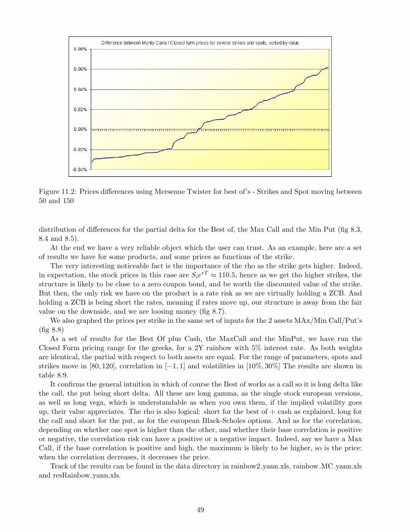
Figure 11.2: Prices differences using Mersenne Twister for best of’s - Strikes and Spot moving between50 and 150

distribution of differences for the partial delta for the Best of, the Max Call and the Min Put (fig 8.3,8.4 and 8.5).

At the end we have a very reliable object which the user can trust. As an example, here are a setof results we have for some products, and some prices as functions of the strike.

The very interesting noticeable fact is the importance of the rho as the strike gets higher. Indeed,in expectation, the stock prices in this case are Sie

rT ≈ 110.5, hence as we get tho higher strikes, thestructure is likely to be close to a zero coupon bond, and be worth the discounted value of the strike.But then, the only risk we have on the product is a rate risk as we are virtually holding a ZCB. Andholding a ZCB is being short the rates, meaning if rates move up, our structure is away from the fairvalue on the downside, and we are loosing money (fig 8.7).

We also graphed the prices per strike in the same set of inputs for the 2 assets MAx/Min Call/Put’s(fig 8.8)

As a set of results for the Best Of plus Cash, the MaxCall and the MinPut, we have run theClosed Form pricing range for the greeks, for a 2Y rainbow with 5% interest rate. As both weightsare identical, the partial with respect to both assets are equal. For the range of parameters, spots andstrikes move in [80, 120], correlation in [−1, 1] and volatilities in [10%, 30%] The results are shown intable 8.9.

It confirms the general intuition in which of course the Best of works as a call so it is long delta likethe call, the put being short delta. All these are long gamma, as the single stock european versions,as well as long vega, which is understandable as when you own them, if the implied volatility goesup, their value appreciates. The rho is also logical: short for the best of + cash as explained, long forthe call and short for the put, as for the european Black-Scholes options. And as for the correlation,depending on whether one spot is higher than the other, and whether their base correlation is positiveor negative, the correlation risk can have a positive or a negative impact. Indeed, say we have a MaxCall, if the base correlation is positive and high, the maximum is likely to be higher, so is the price:when the correlation decreases, it decreases the price.

Track of the results can be found in the data directory in rainbow2 yann.xls, rainbow MC yann.xlsand resRainbow yann.xls.

49

Figure 11.3: Distribution of delta differences Monte Carlo/Closed Form for the Best of, for differentspots and strikes

Figure 11.4: Distribution of delta differences Monte Carlo/Closed Form for the Max Call, for differentspots and strikes

50

Figure 11.5: Distribution of delta differences Monte Carlo/Closed Form for the Min Put, for differentspots and strikes

Figure 11.6: Best of price as a function of the strike: T = 1, σ1 = σ2 = 20%, r = 10% andS1 = S2 = 100

51

Figure 11.7: Best of rho as a function of the strike: T = 1, σ1 = σ2 = 20%, r = 10% and S1 = S2 = 100

Figure 11.8: Max/Min Call/Put’s as functions of the strike: T = 1, σ1 = σ2 = 20%, r = 10% andS1 = S2 = 100

52

Partial Delta Partial Gamma Partial Vega Rho CorrelBest Of Min 0.32 0.00 0.01 -42.39 -16.40

Max 109.53 520.09 18.74 0.00 10.45MaxCall Min 0.00 0.00 0.06 8.84 -15.59

Max 116.93 519.42 18.91 28.28 7.84MinPut Min -61.63 0.10 0.02 -21.71 -16.40

Max 0.00 192.37 4.33 -2.29 3.82

Figure 11.9: A few results on the greeks - Min and Max values noticed for reasonable parameters

11.5 Choices

We chose not to use dividends in the whole project (from Black-Scholes to the rainbows), but wecould easily add them in our closed forms as shown earlier, and to Monte Carlo by adjusting thedrift class and removing the dividend rate from the risk free growing rate. We had to amend theDrift/Gaussian/Random/MCEngine/Payoff classes in default constructors so as to avoid passing valar-rays all the time and be more efficient: with non path dependant options, the only simulated point isthe terminal one, so a one period model does not need to pass arrays of one parameter.

The choice was made to enable n assets, so that adding a new type does not change the wholestucture of the class, and just needs adding the relevant pricing method to the class.

11.6 Validation

11.6.1 Approach

To validate the results of this part even further, the only possibility was to recreate a monte carlo pricerwith an easire structure, making it easier not to make bugs inside. For this we chose to dewvelop it inVBA. Since we also had closed formulas for some options we were quite confident with the results ofour C++ pricer, but for some options, it was comfortable to get the same results with another pricer.This pricer can be found in the data part of our project under the name RainbowMCTests simon.xls.The user can input his own parameters in the spreadsheet, choose the number of simulations to run, amaximum acceptable error and can then run the simulation. One has to be careful since the programis much slower in VBA. After the calculation is finished there is a cell indicating TRUE on a yellowbackground if all tests passed or FALSE on a red background if some failed. We were happy tocheck that all results were really good and very close to our c++ results, even for a small number ofgenerations.

53

Chapter 12

Part J: Convertible Bonds

Developer: Aloke MukherjeeValidator: Jospeh Perez

12.1 Requirements

A convertible bond behaves as a hybrid between a bond and a stock because in addition to the principalguarantee and coupons it can also be converted into a specified number of shares of stock at giventimes. As the chance of converting increases due to stock price appreciation the price of convertiblebonds will behave more like the stock. If the chance of converting is low then the convertible’s pricewill be more affected by interest rates and its behaviour is more bond-like.

This ”early-exercise” feature of convertible bonds makes it difficult to model with Monte Carlosimulation. Instead a binomial tree is used to model the underlying stock price. The convertible bondis then evaluated at leaf nodes as the maximum of the par value and the conversion value and thesevalues are propagated back to the tree’s root.

An additional complication is the callability and putability features of convertible bonds. Calla-bility allows the issuer to call back the bond at a set price. Putability conversely allows the owner theput the bond back to the issuer at a set price. This optionality can also be modelled in the binomialtree by evaluating at each step whether it is optimal for either party to exercise their option.

12.2 Design

We constructed a binomial tree class which can store the intermediate stock process and claim processvalues. At instantiation this class uses the yield curve and the stock’s price and volatility to calculateand cache the magnitude of each up and down jump. The Cox-Ross-Rubinstein values are used -namely up moves are eσ

√t and down moves are the reciprocal of this. The probability of an up

move is the difference between the riskfree value at the next node and the down value divided bythe difference between the up and down values. The probability of a down move is the complement.We use the yield curve’s ability to compute forward discount factors to compute discount factors andprobabilities for each step of the tree. If a flat yield curve is specified these will all be the same butthe design allows the use of a more realistic yield curve.

Evaluation of the claim process is based on the same technique used in the Monte Carlo simulation:different ”Engine” methods are defined in the binomial tree class which can be used to evaluate differentclaim processes. The engine uses a standard PayOff object used throughout the project to evaluatethe claim at terminal nodes. The engine applies risk-neutral probabilities to discount the payoff as wellas evaluating the different options at each node. For convertible bonds this decision can be expressed

54

asmax(Conversion value, min(Bond V alue, Call Price), Put Price)

The convertible bond class’ main task is to contain the various attributes of the convertible suchas conversion ratio, call price, put price, the underlying asset and underlying risky bond. Mostimportantly it takes care of instantiating and invoking binomial trees to calculate the price of theconvertible as well as the associated greeks.

12.3 Choices

We made a few simplifying assumptions due to time constraints. The design is such that incorporatingthese factors in the future should be straightforward. As in other sections of the project we ignorethe effect of dividends. The bond component of the convertible is assumed to be a zero-coupon bond(e.g. no coupons). We assume that callability and putability decisions are taken at each node in thebinomial tree. Credit considerations are also neglected although the convertible currently does take acredit curve in its constructor. This means that the ”bond floor” will be slightly higher than expected.

The convertible bond class inherits from the riskybond class. This makes sense intuitively becauseof its bond-like characteristics and the fact that convertible’s are issued by companies that have defaultrisk. The binomial tree is implemented using arrays of valarrays. This simplifies instantiation andother operations requiring access to the interior nodes.

The convertible bond greeks were calculated by comparing the given convertible bond with a newlyinstantiated convertible bond with appropriately shifted parameters. The greeks calculated were:

• delta - change in convertible price corresponding to a change in the price of the underlying asset.

• gamma - change in delta corresponding to a change in the price of the underlying asset.

• rho - change in convertible price corresponding to a change in the underlying interest rate. Thiswas modelled by using the ability to create a ”shifted” risky bond with the yield curve shiftedup by a given number of points. Also referred to as interest rate delta.

Convertible greeks are often computed with respect to parity, the product of conversion ratio andstock price. Parity delta can be computed by dividing delta by the adjusted conversion ratio and paritygamma by dividing gamma by the square of the adjusted conversion ratio. The adjusted conversionratio is simply the conversion ratio scaled down by (face value / 100). This allows the parity greeksto be compared among bonds of differing face values.

Interestingly, convertibles have a few other greeks specific to them. One of these is omicron, thechange in convertible price due to a change in credit spreads. Unfortunately, since we did not modelcredit spreads in our pricing model we were not able to compute this value.

12.4 Unit tests

The binomial tree class was verified by comparison with the Matlab implemented binomial tree (dis-cussed also in the Black-Scholes section). The Matlab code can be found in the data directory in thefile bintree.m.

In addition we verify in the C++ test that the most extreme leaf nodes have the expected valuesgiven the specified volatility. Finally we implemented an engine to evaluate a European claim. Thisvalue was compared to the results of the closed-form equations and Monte Carlo simulation. Thebinomial tree also has an output operator which allows all the interior nodes of both the stock andclaim process to be displayed. This was invaluable in verifying correct operation.

The convertible bond was tested by trying out an example similar to that outlined in Hull example21.1 (6th edition). This example has similar assumptions to those outlined above except for the

55

modeling of default. We find the price from our model is slightly higher than that computed in Hulldue to this simplification. By inspecting interior nodes we verified that the appropriate action (e.g.call, put, conversion) predicted in Hull was chosen at each interior node. We also priced the Atmelconvertible bond described in the lecture notes. Since we did not model all the parameters and didnot know the underlying yield curve the results did not match exactly but they appeared to be in theballpark. The output of these tests can be seen in the convertible test function accessible from thetest selection of the menu.

The convertible bond was also validated using Zhi Da’s Convertible Bond Calculator(see http://www.kellogg.northwestern.edu/faculty/da)which can be easily programmed to match the assumptions in our model. This is discussed further

in the validation section but we find the results to match well. A copy of the calculator can be foundin the data directory as CBCalculator.xls. It has been slightly altered to not convert the specifiedrate into a continuous rate. It has also been loaded with the data used in the first example in theconvertible bond test.

12.5 Performance

The binomial tree implementation can be optimized by a variety of means. Some of these are outlinedin the paper ”Nine Ways to Implement the Binomial Method for Option Valuation in MATLAB”(http://epubs.siam.org/sam-bin/getfile/SIREV/articles/39326.pdf). The most important improve-ment suggested is using high-level operations on arrays. Matlab is specialized to deal with such arrayshowever the same logic can be applied to C++ when using valarrays since valarrays are optimized tohandle batch operations on all elements as in Matlab. Space usage is also inefficient in our implemen-tation increasing with the square of the number of steps. The same calculations can be implementedusing a single flat array by replacing the elements as we work backwards through the tree.

The convertible bond makes some use of caching. It will cache the price and greeks for the mostrecently requested date. An improvement here would be to implement some kind of hashmap allowingthese values to be cached for multiple dates. Currently for example if requests were made sequentiallyat different dates, the caching functionality would not help.

12.6 Validation

12.6.1 Approach

To validate we run pricing of convertible bond with VBA. The excel file is CBcalculator.xls (detailsabove). The principle for pricing is also to use a binomial tree. Giving the same parameters we gotthe same results.

56

Figure 12.1: Results of pricing of a convertible bond with VBA

Figure 12.2: Results of pricing of a convertible bond with our project

57

Chapter 13

Part K: Variance Swaps

Developer: Simon LegerValidator: Aloke Mukherjee

13.1 Requirements

In this section, we use a portfolio of European options to compute the value of a variance swap. Wewrite methods to compute the value of such swaps.

13.2 Design

The value of a variance swap is computed according to the theoritical formula. There is in fact aformula to compute the value of a variance swap under no-arbitrage assumption which is not the casefor volatility swaps for instance.

13.3 Approach

To create a variance swap object, we use the OptionStrategy design built in part A and we pass apointer to such an object, with a maturity and a forward price since it is all we need to compute thevalue.

13.4 Choices

We decided to create all information required in the constructor of the object and store them likepointers so we have a function getPrice() which calculates the price according to the values stored andaccording to the following formula :

Price =2T

(∫ F

0

1K2

P (K)dK +∫ ∞

F

1K2

C(K)dK

)where T is the maturity of the contract, F is the forward price, P (K) is the price of the put and

C(K) the price of a call with strikes K.

13.5 Unit tests

Test on the VIX index : To test the accuracy of the variance swap implementation we create a portfolioof puts and calls options, by using the OptionStrategy class. We take a minimum and a maximum

58

strike and a step for this and we create a bench of options with these strikes, calls if the strike ishigher than the forward value of S&P and puts in the other case. With a minimum strike of 500, amaximum strike of 3500, a step of 10, we take a spot at 1200, the one month interest rate is around4.3the current value of the VIX index which is around 11.

13.6 Validation

13.6.1 Approach

For this section’s validation, the more efficient way to test the accuracy of the results provided bt thevariance swaps part was to build the formula in an Excel spreadsheet built from prices of options,both calls and puts whose values have been calculated with the Black Scholes closed formula. We thencompute the same price as in the example provided in the unit test part and we found the same result.As well as for the VIX index, where we have very similar prices to exact value of the index found onthe CBOE web site, such that we can consider that the results provided by this class are good.

59

Chapter 14

Part L: Exotic Products

Developer: Simon LegerValidator: Yann Renoux

14.1 Requirements

In this section, we design and write a monte carlo based framework that will allow us to price a varietyof exotic products. Our framework has to be able to generate simulateed paths for one asset, for everymonth for five years. Once we have these paths we apply a corresponding payoff formula on the set ofpaths to get a price for European style products with the following features :

• Asian options

• Barrier options

• Look back options

• Cliquet

14.2 Design

To design this part, we chose to create just one class which is going to use the monte carlo basedframework developed in part A. Then we add methods to get the price of the exotic according to atype associated with a given payoff and methods to get the greeks.

14.3 Approach

The Monte-Carlo framework meets all requirements for this part. It is even more general since we areable to generate as many intermediate points as we want for given dates. As all these products haveonly one underlying, we are able to use the Sobol generator for them and we get better prices with it.

14.4 Choices

This section is in the ”Exotics” class. It takes in the constructor everything it requires to computethe price, they are stored as pointers also to make it faster and it also needs a type, which is the kindof products you need. Here are all possibilities :

enum exoticsType

• AsianCall,

60

• AsianPut,

• RevLookbackCall,

• RevLookbackPut,

• FlooredCliquet,

• CappedCliquet,

• CollaredCliquet,

• BarrierCall,

• BarrierPut

;If one wants to add other products, this is very easy since he only needs to add a case in the

getPrice() function and write a main montecarlo function for this and applying a new payoff. Wealso provide the greeks by finite difference method. For this one needs to be careful since we have toapply the same random numbers to the paths to get correct greek values, other wise the Monte Carloapproximation error is greater than the difference given by the change on underlying, vol... dependingon the greek value. For this we just reset the seed of the generator, which for Sobol is equivalent torecreate orginal vectors for it, which is done by creating a new instance of the generator. This is nota problem in terms of speed since we do not do any computation that is not required.

14.5 Validation

14.5.1 Approach

As these exotic derivatives do not have any closed form solution, our only alternate method to validatethe prices is to use an independant Monte Carlo engine and recompute some prices for each optionwith different sets of parameters. As we had already designed a VBA based Monte Carlo tool, were-used it to adapt it to the exotic payoffs, this time on a single asset but with path dependancy. Herethen the simulated path should be a natural divider of the number of points needed in the payoff. Sayfor example that we consider a Reverse Look-Back of 2 years, with one added observation date afterthe first year, we need to simulate the path the end of year 1 AND the end of year 2 to be able tomaximize the underlying price on these two dates. The rest follows usual pricing methodology, i.e.making sure we simulate the price with normal independant samples if we have several dates, andrecombine the price with the correct drift and volatility for the brownian motion. In practise the drift

would be exp((r − 12σ2) T

nb Obs) and for the gaussian exp(σ√

Tnb Obs) from one observation date to the

other. For the following inputs:

Spot 100K 100σ 20%r 5%T 1nPaths 100, 000

We have checked the prices for some of the products – Monte Carlo simulation in VBA is reallyslow, so we could not do a broad range as for the rainbows. All available exotics were done exceptthe cliquets. We checked that for a single date, the Asians and Reverse Look Backs lead to the Black

61

Scholes closed form solutions, which is the case. As we increase the number of dates, the maximum onthe path should be higher, hence the ReverseLook Back Call should be more expensive with more dateswhile the put version should be less expensive. For the Asians, the averaging smoothes the extremevalues hence for 2 dates and more, the price is lower than the associated Black Scholes EuropeanCall/Put. For the one-touch options, the more the dates, the more likely we are to touch the barrier,hence a higher price.

Terreneuve ExcelnDates 1 2 1 2RevLookBackCall 10.425 12.169 10.425 12.208AsianCall 10.425 8.108 10.432 8.115RevLookBackPut 5.578 2.855 5.596 2.894AsianPut 5.578 4.451 5.544 4.486One Touch Call 0.532 0.641 0.533 0.640One Touch Put 0.419 0.546 0.418 0.543

Black Scholes Call 10.451Black Scholes Put 5.574

The remarks on the moves of prices with the number of dates are met, as well as Black-Scholescomparison. The prices for only 100, 000 simulations are in line within 1.4% (for the reverse lookback put on 2 dates), so we can consider that this object passes the validation test. Result file indata/exotics yann.xls

14.5.2 Pitfalls

No major pitfall was found. As for the other classes, the on-going validation process enabled to discoversome bugs that were fixed, and also for more than one date, do not use Sobol in one dimension.

62

Chapter 15

Part M: Portfolio

Developer: AllValidator: All

15.1 Requirements

In this section we design and write a framework that represents the characteristics and behavior ofportfolios and their values and risk under different types of market scenarios. Each portfolio has a nameand a currency. All relevant financial information about the portfolio such as its value, profit/loss,and risk is expressed in the portfolio currency. The portfolio will contain a number of securities whosepositions, profit loss and risk the objects will manage. For each security in the portfolio our frameworkwill provide the security name, cost basis, current price, price currency amount, current value, profitloss. Each security will have a risk profile called its risk map. The risk map describes the variation inthe value of the security for changes/shifts in risk factors. The framework will allow scenario analysisfor the portfolio. We should implement methods for the following :

• Current value of the security

• Profit loss for the security

• Profit loss for the portfolio

• Current value of the portfolio

• Import portfolio information from a file

• Import list of securities from a file

• Import risk map of a security from a file

• Import scenario list from a file

• Value of the portfolio for a single risk factor risk scenario

• Profit/Loss report

• Portfolio analysis report

• Value at risk for the portfolio

63

15.2 Choices

As mentionned by Pr Laud in the last week, we did not try to do the VaR. Though the frameworkof the project would have easily permitted it, we have chosen to focus on validating correctly all thedelivered structures rather than delivering more but not being sure of the reliability of the products.

The design enables the structure to be able to handle the requirements as if bears all the informationon all the products we developped in this project.

15.3 Approach

The portoflio class in the C++ project just takes a name and a currency and provides the user of theprogram with methods to add each type of security we have, namely :

• OptionStrategy, which is already a portfolio of BlackScholes object

• Rainbow options

• Exotic options

• Vanilla swap

• Variance swap

• Bond

• Asset

There is also a method to compute the value of the portfolio and to get the absolute risk fordifferent sorts of scenarios, similar to the greeks for the options.

15.4 Choices

Each security is stored in the portfolio in valarrays of pointers to these objects, since we dont want tomake a copy of already existing objects. For each security we also have a quantity, in order to avoidto copy them many times in the portfolio.

We also provide similar methods to greek values for the portfolio, giving a risk value for differentkinds of risks, which are calculated by calling these methods from the security class, if this one exists.For example there is no sensibility to volatility for a bond or a vanilla IR swap, but each security hasa sensibility to the interest rate or to time.

15.5 Validation

All structures were validated in the other sections, and tested. This one just goes through all thevalarrays of the products to add them (deleting is adding the opposite quantity) and return the valueof the portfolio, and its greeks with which we could output the stress loss or PnL report based on themoves of any market parameter.

64

Chapter 16

Conclusion

This report is quite long, so we will not spread pages as a conclusion.We obviously learnt a lot with this project, as we have tried to share a lot on the issues we were

facing on a daily basis. The number of emails of the list that were sent per day is amazingly huge.It leads us to the fact that the team work was excellent on this project, and the use of CVS and

Skype for conference calls – we said we thanked the nerds that invented the internet ! – made surethat from the beginning the objects were plugging together exactly. We avoided much of the lastminute pain in doing that.

We hope the project is in the most deliverable state as possible, even if the user cannot ”consolely”play with all the products, the code is there anyways.

Future WorkThis project clearly illustrates the complexity of the universe of financial products. Additionally,

there can be many approaches to modelling each product. In this project we have implemented someof the most popular modeling techniques including closed-forms, Monte Carlo simulation and binomialtrees, and not just in C++ but also in Excel and Matlab! As developers attempting to work withthis variety, the first and foremost imperative is ”get it working”. We’ve learned that this is not asimple task: to begin with how will you even know it is working? But once you’ve conquered thatpeak, the sky is the limit: approaches can be changed, parameters altered, models made more precise,computations made more efficient. This project has been a great experience because it has exposedus to a wide variety of approaches and techniques. And having not died from exposure, we can seefrom these heights how much exciting work there is left to do!

– The Terreneuve Team that will now celebrate as a team the end of the semester.

65