Computing Delay with CouplingUsing Timed Automata

Serdar Tasiran, Yuji Kukimoto, Robert K. Brayton

Department of Electrical Engineering & Computer Sciences

University of California, Berkeley

,

Overview

A timed-automaton-based method for computing the delay of a combinational circuit.

Outline: Why do we need a new method?

Timed automata Representing sets of waveforms Delay models Hierarchical representation

The complexity problem Hierarchical approach Timed “image computation” Heuristics

Status and Future Work

Why do we need a new method?

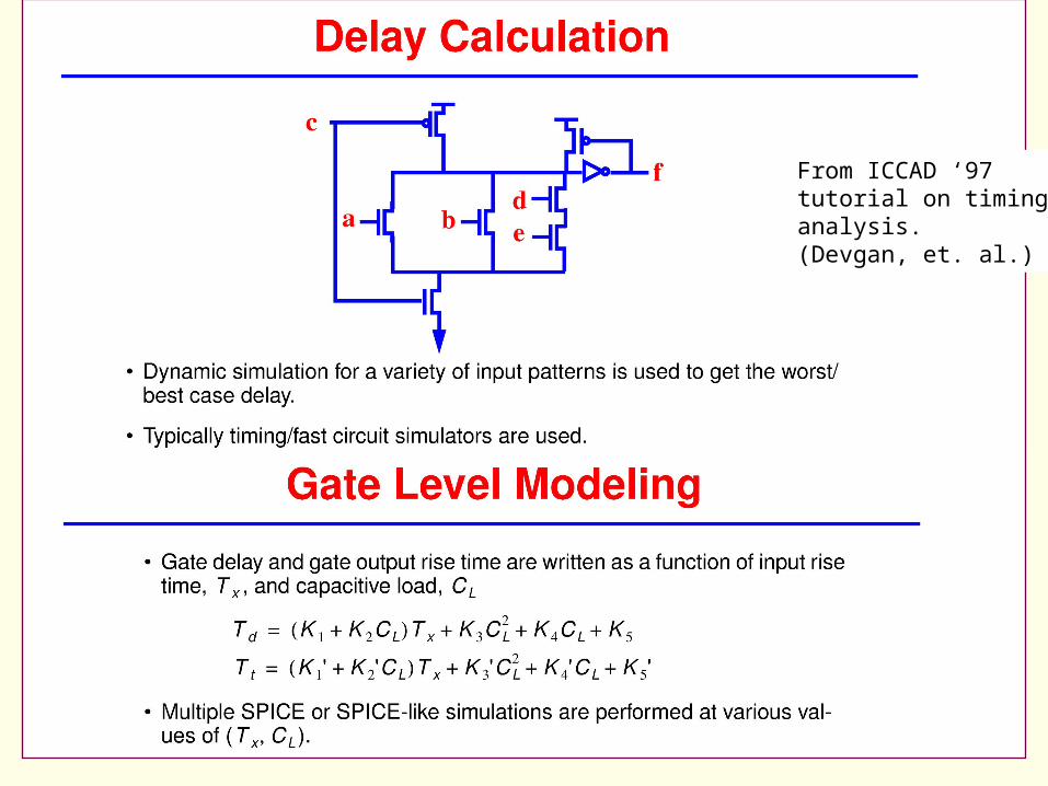
From ICCAD ‘97tutorial on timing analysis.(Devgan, et. al.)

GOAL: Delay analysis tool that can handle ~100s of gates.

Must handle sophisticated delay models Dynamic logic: Complex gates

Delay depends on relative arrival times and values of inputs. Cross-talk between nodes, wires running parallel.

What about static analysis and simulation?

Simulation Number of possible input patterns exponential in # of inputs:

For large circuits, infeasible to simulate all patterns. Delay not guaranteed unless all patterns are simulated.

From ICCAD ‘97tutorial on timing analysis.(Devgan, et. al.)

Static Analysis Topological delay does not account for cross-talk. Assuming worst case cross-talk on all wires is too conservative.

OUR APPROACH Timed automata serve as delay models for circuit components Delay parameters obtained by

Simulation Analytical methods

Formal timing verification used to compute delay All patterns covered; delay guaranteed.

From ICCAD ‘97tutorial on timing analysis.(Devgan, et. al.)

OUR METHOD

GOOD

MEDIUM

YES

Timed Automata

Clocks (timers): real-valued variables, increase at same rate.

For each location an output assignment an invariant: a clock predicate.

Clock predicate: Positive Boolean combination of x d and x d.

i o

2 delay 3

i = 1, x 0

i =0, x 3

o = 0 2 x 3 x 3o = 0 o = 1

Initial

2

3

i

o

reset x

From ICCAD ‘97tutorial on timing analysis.(Devgan, et. al.)

Timed Automata as Delay Models

i =0, x 0

i =1, x dfall,max

Initial

o = 1

i = 1, x 0

i = 0, x drise,max

o = 0

x dfall,max

o = 1

o = 0

Initial

x dfall,max

dfall,min x

x drise,max

drise,min x

x drise,max

Example: Inertial delay model for a wire segment.

Determine dfall,min , dfall,max , drise,min , drise,max using simulation for various input patterns.

Construct timed automaton model with these parameters.

More sophisticated delay models can be expressed using timed automata.

Delay of this gate depends on Old and new values of a, b, c, d, e Relative arrival times of a, b, c, d, e

Modeling this circuit with [dmin, dmax]is too coarse.

Modeling Cross-talk With Timed Automata

f and g are look-up tables f increases x

wire k takes less time to rise g decreases x

wire k takes longer to rise

f and g are determined by simulation or analytical computation and by conservative discretization.

Choosing a smaller time unit gives better accuracy but increases complexity.

ok = 0, ck = risingok = 0, ck = stable

ok = 0, ck = rising

ok = 0, ck = rising

ok = 1, ck = stable

x drise,max

drise,min x

x drise,max

drise,min x

x drise,max

drise,min x

x drise,max

x drise,max

x drise,max

i = 1x 0

cj = risingx f(x)

cj = fallingx g(x)

wire k

aggressor wire j

x f(x)

[0,3] [0,5]

[4,7] [6,10]

[8,10] [9,12]

[11,15] [12,17]

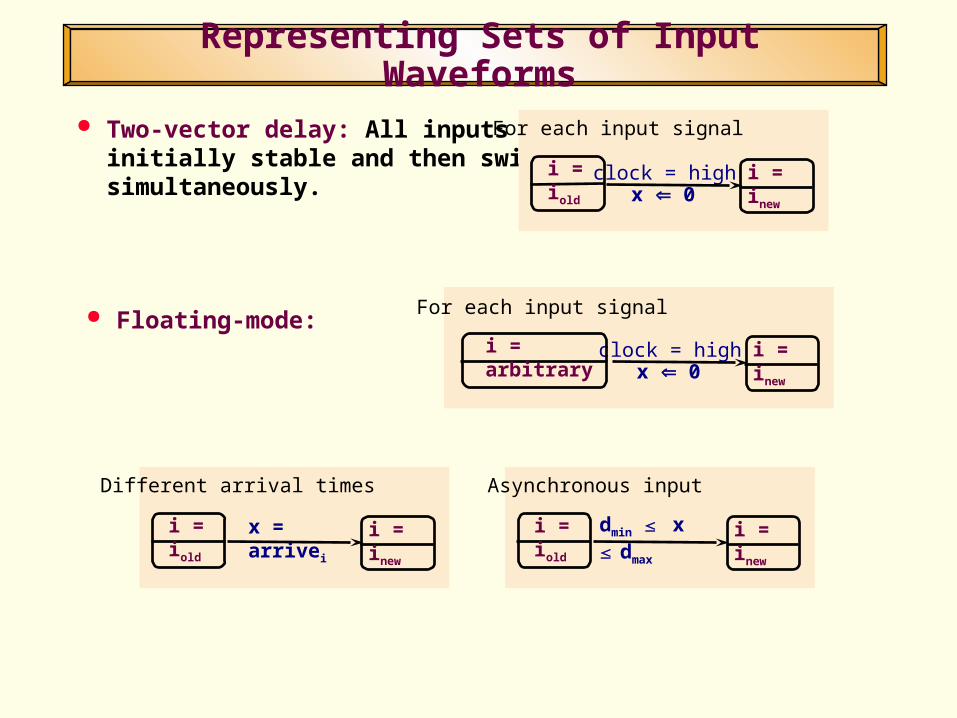
Representing Sets of Input Waveforms

Two-vector delay: All inputs areinitially stable and then switchsimultaneously.

clock = highi = iold i = inew

For each input signal

x 0

i = iold i = inewx = arrivei

Different arrival times

i = iold i = inewdmin x dmax

Asynchronous input

Floating-mode:clock = highi = arbitrary i = inew

For each input signal

x 0

Composition of Timed Automata

o p

3 delay 5

o= 0, y 0

o=1, y 5

p= 1 3 y 5 y 5p= 1 p= 0

Initial

B1 B3B2

B

i o

2 delay 3A

i = 0, x 0

i =1, x 3

o = 1 2 x 3 x 3o = 1 o = 0

Initial

A1 A3A2

A || B

i o p

o=1, p=1

Initial

(A1 , B1) i = 0, x 0

i =1, x 3

o=1, p=1

(A2 , B1)

x 3

2 x 3 o=0, p=1

(A3 , B2)

y 5y 0

3 y 5o=0, p=0

(A3 , B3)

Variable Hiding (Smoothing)

A||B

i o p

o=1, p=1

Initial

(A1 , B1) i = 0, x 0

i =1, x 3

o=1, p=1

(A2 , B1)

x 3

2 x 3 o=0, p=1

(A3 , B2)

y 5y 0

3 y 5o=0, p=0

(A3 , B3)

p=1

Initial

(A1 , B1) i = 0, x 0

i =1, x 3

p=1

(A2 , B1)

x 3

2 x 3 p=1

(A3 , B2)

y 5y 0

3 y 5p=0

(A3 , B3)

(o) (A||B)

i p

Hierarchical View of Circuits

Higher Level Block =

(internal signals) ( Component 1 || Component 2 ||... Component n )

“COMPOSE-SMOOTH”

To obtain simpler, smaller representation for HLBwe often need to

Apply conservative abstraction, I.e., overapproximate behavior of product automaton.

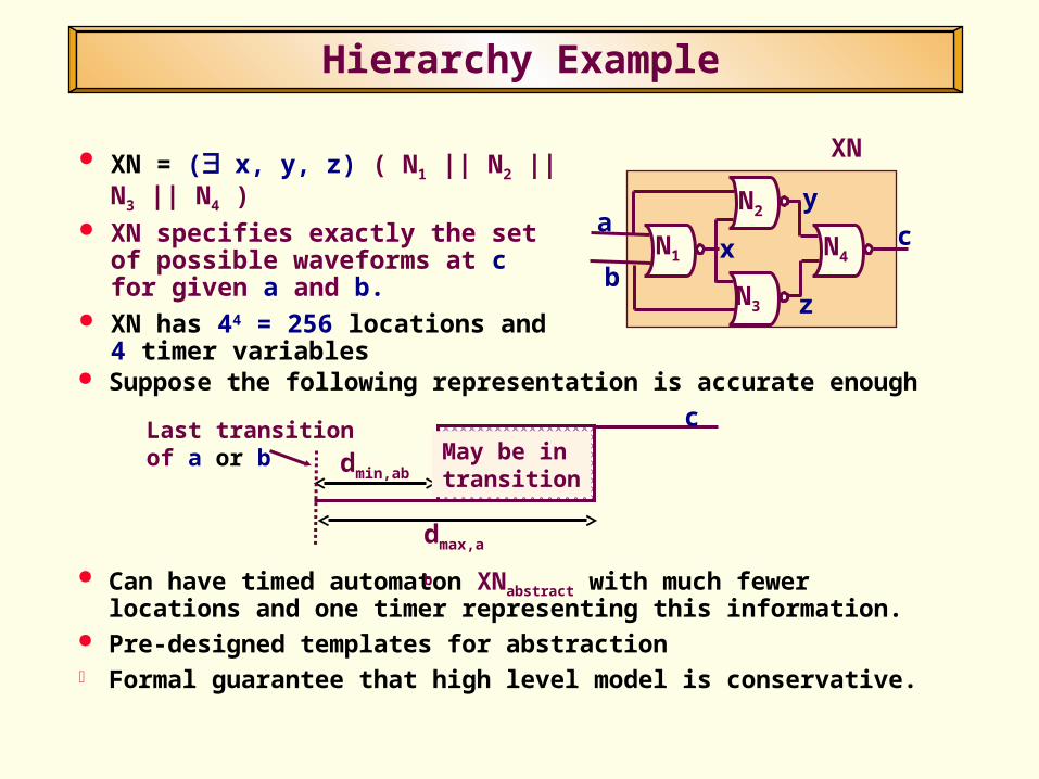
Hierarchy Example

XN = (x, y, z) ( N1 || N2 || N3 || N4 ) XN specifies exactly the set of

possible waveforms at c for given a and b.

XN has 44 = 256 locations and 4 timer variables

N4N1

N2

N3

XN

x

y

z

a

b

c

Suppose the following representation is accurate enough

Can have timed automaton XNabstract with much fewer locations and one timer representing this information.

Pre-designed templates for abstraction Formal guarantee that high level model is conservative.

May be intransition

dmin,ab

dmax,ab

Last transitionof a or b

c

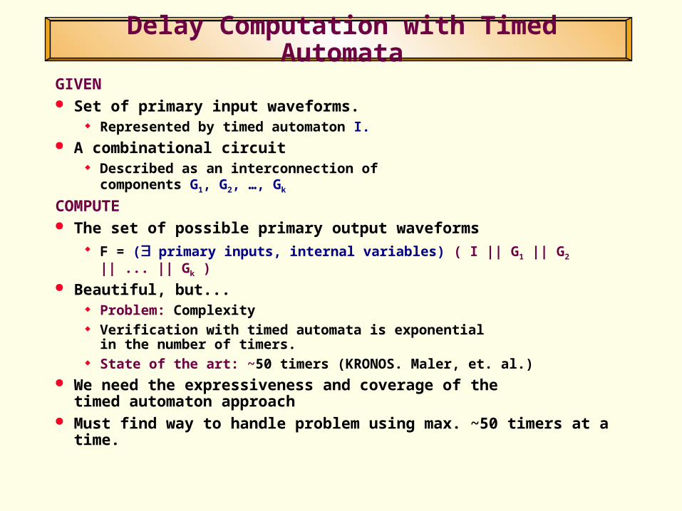
Delay Computation with Timed Automata

GIVEN Set of primary input waveforms.

Represented by timed automaton I. A combinational circuit

Described as an interconnection of components G1, G2, …, Gk

COMPUTE The set of possible primary output waveforms

F = (primary inputs, internal variables) ( I || G1 || G2 || ... || Gk ) Beautiful, but...

Problem: Complexity Verification with timed automata is exponential

in the number of timers. State of the art: ~50 timers (KRONOS. Maler, et. al.)

We need the expressiveness and coverage of the timed automaton approach

Must find way to handle problem using max. ~50 timers at a time.

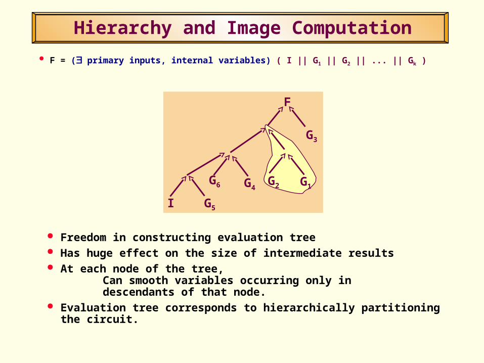
Hierarchy and Image Computation

F

G3

G5

G6 G4

I

F = (primary inputs, internal variables) ( I || G1 || G2 || ... || Gk )

Freedom in constructing evaluation tree Has huge effect on the size of intermediate results At each node of the tree,

Can smooth variables occurring only in descendants of that node.

Evaluation tree corresponds to hierarchically partitioning the circuit.

G2 G1

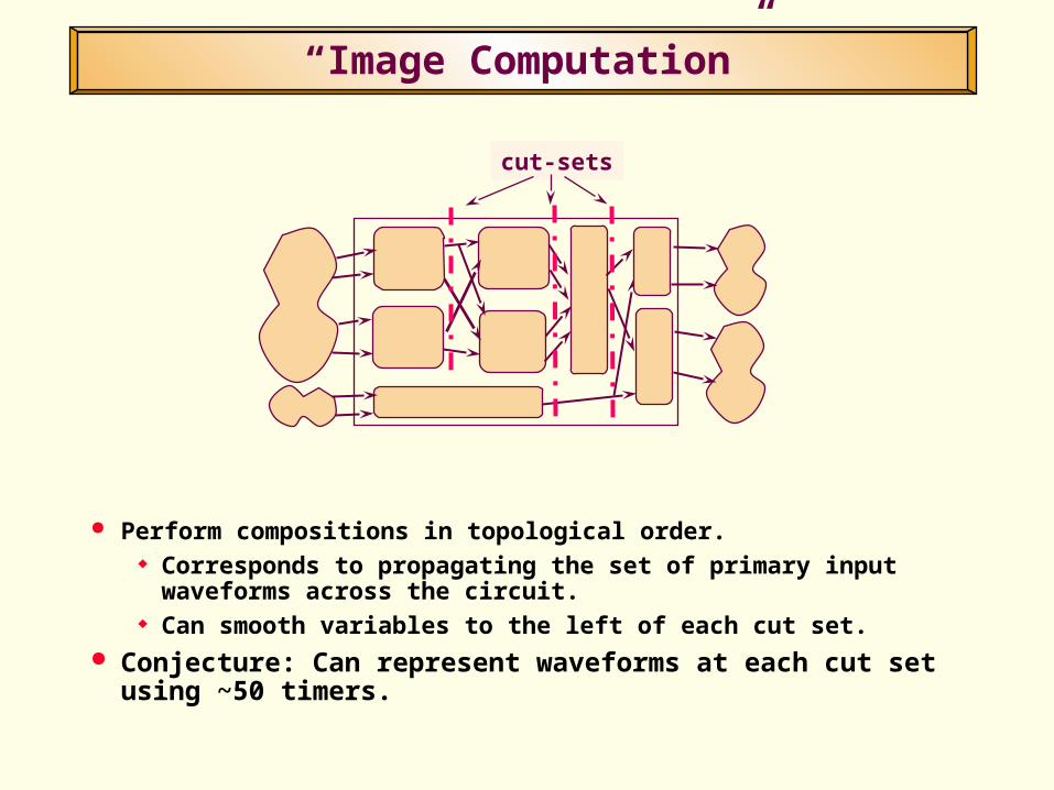
“Image Computation”

cut-sets

Perform compositions in topological order. Corresponds to propagating the set of primary input

waveforms across the circuit. Can smooth variables to the left of each cut set.

Conjecture: Can represent waveforms at each cut set using ~50 timers.

Compose-Smooth-Abstract

Key subroutine for this approach.

ALGORITHM: Take product of component automata Smooth internal variables

Perform “untimed reachability analysis” on product automaton Ignore timing information on edges Perform reachability analysis considering logical functionality only Conservative: Less minimization than timed analysis. BUT efficient: Complexity does not depend on timers.

Apply timer minimization algorithm of [Daws, Yovine, RTSS ‘96]. Identifies:

Timers that can’t be simultaneously active Timers that have equal values Important observation: Only the # of simultaneously active, unique timers

affects complexity. Conjecture: For shallow DSM circuits, few timers should be required.

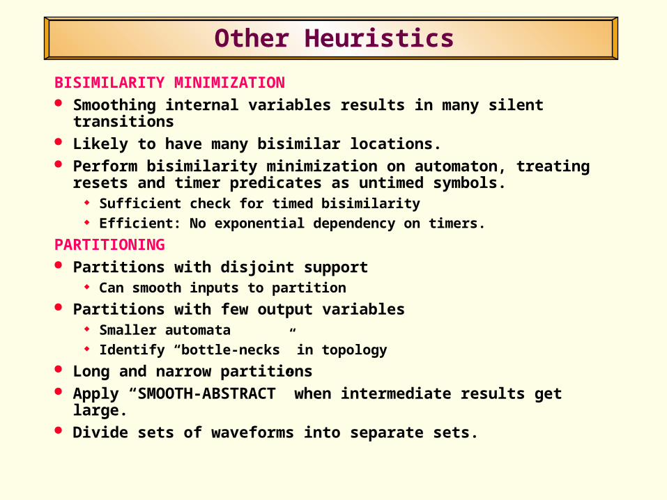
Other Heuristics

BISIMILARITY MINIMIZATION Smoothing internal variables results in many silent transitions Likely to have many bisimilar locations. Perform bisimilarity minimization on automaton, treating resets

and timer predicates as untimed symbols. Sufficient check for timed bisimilarity Efficient: No exponential dependency on timers.

PARTITIONING Partitions with disjoint support

Can smooth inputs to partition Partitions with few output variables

Smaller automata Identify “bottle-necks” in topology

Long and narrow partitions Apply “SMOOTH-ABSTRACT” when intermediate results get large. Divide sets of waveforms into separate sets.

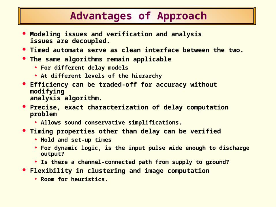
Advantages of Approach

Modeling issues and verification and analysis issues are decoupled.

Timed automata serve as clean interface between the two. The same algorithms remain applicable

For different delay models At different levels of the hierarchy

Efficiency can be traded-off for accuracy without modifying analysis algorithm.

Precise, exact characterization of delay computation problem Allows sound conservative simplifications.

Timing properties other than delay can be verified Hold and set-up times For dynamic logic, is the input pulse wide enough to discharge output? Is there a channel-connected path from supply to ground?

Flexibility in clustering and image computation Room for heuristics.

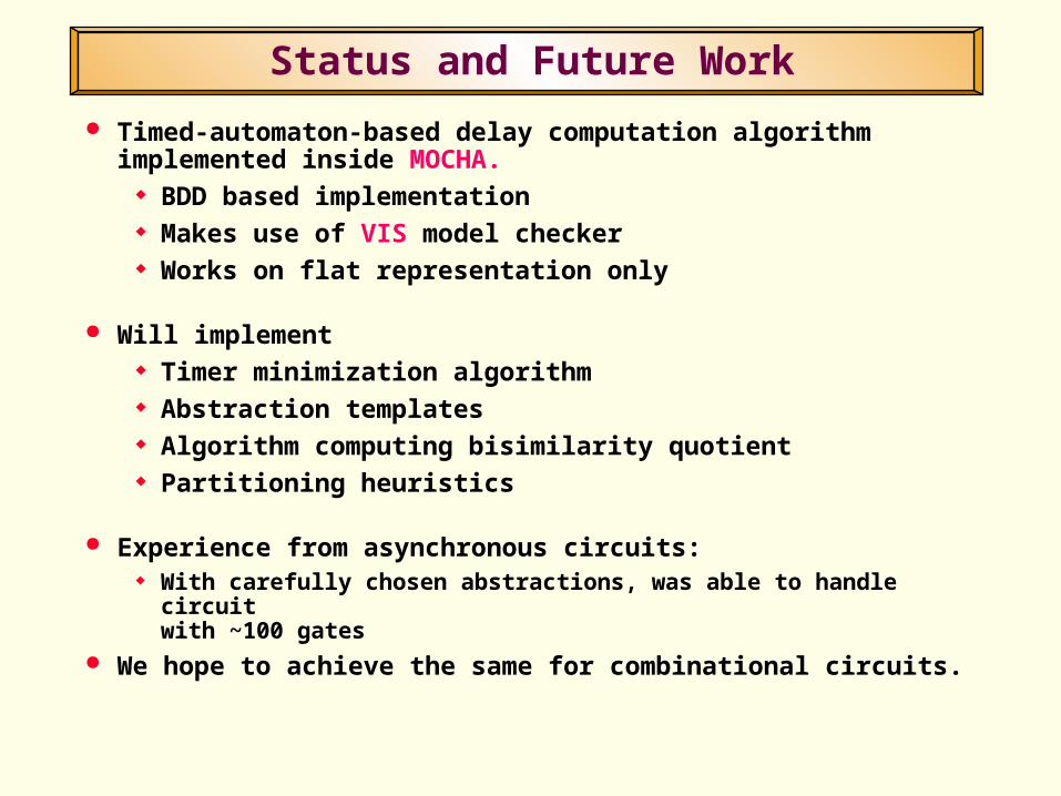
Status and Future Work

Timed-automaton-based delay computation algorithm implemented inside MOCHA.

BDD based implementation Makes use of VIS model checker Works on flat representation only

Will implement Timer minimization algorithm Abstraction templates Algorithm computing bisimilarity quotient Partitioning heuristics

Experience from asynchronous circuits: With carefully chosen abstractions, was able to handle circuit

with ~100 gates We hope to achieve the same for combinational circuits.

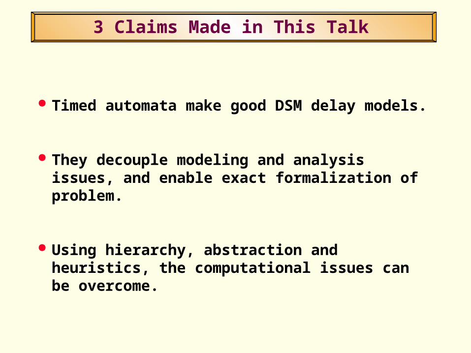
3 Claims Made in This Talk

Timed automata make good DSM delay models.

They decouple modeling and analysis issues, and enable exact formalization of problem.

Using hierarchy, abstraction and heuristics, the computational issues can be overcome.