Computer - Deslab 2017deslab.mit.edu/DesignLab/tmaekawa/book/mathe.pdf · 2002-03-09 · Nic holas...
423
Transcript of Computer - Deslab 2017deslab.mit.edu/DesignLab/tmaekawa/book/mathe.pdf · 2002-03-09 · Nic holas...
Nicholas M. Patrikalakis Takashi Maekawa
Shape Interrogation for Computer
Aided Design and Manufacturing
SPIN Springer's internal project number, if known
Mathematics { Monograph (English)
June 26, 2001
Springer-Verlag
Berlin Heidelberg NewYork
London Paris Tokyo
HongKong Barcelona
Budapest

Preface
Objectives and FeaturesShape interrogation is the process of extraction of information from a geo-
metric model. Shape interrogation is a fundamental component of ComputerAided Design and Manufacturing (CAD/CAM) systems and was �rst used insuch context by M. Sabin, one of the pioneers of CAD/CAM, in the late six-ties. The term surface interrogation has been used by I. Braid and A. Geisowin the same context. An alternate term nearly equivalent to shape interro-gation is geometry processing �rst used by R. E. Barnhill, another pioneer ofthis �eld. In this book we focus on shape interrogation of geometric modelsbounded by free-form surfaces. Free-form surfaces, also called sculptured sur-faces, are widely used in scienti�c and engineering applications. For example,the hydrodynamic shape of propeller blades has an important role in marineapplications, and the aerodynamic shape of turbine blades determines theperformance of aircraft engines. Free-form surfaces arise also in the bodies ofships, automobiles and aircraft, which have both functionality and attractiveshape requirements. Many electronic devices as well as consumer productsare designed with aesthetic shapes, which involve free-form surfaces.
When engineers or stylists design geometric models bounded by free-formsurfaces, they need tools for shape interrogation to check whether the de-signed object satis�es the functionality and aesthetic shape requirements.This book provides the mathematical fundamentals as well as algorithms forvarious shape interrogation methods including nonlinear polynomial solvers,intersection problems, di�erential geometry of intersection curves, distancefunctions, curve and surface interrogation, umbilics and lines of curvature,geodesics, and o�set curves and surfaces.
The book can serve as a textbook for teaching advanced topics of geomet-ric modeling for graduate students as well as professionals in industry. It hasbeen used as one of the textbooks for the graduate course \ComputationalGeometry" at the Massachusetts Institute of Technology (MIT). Currentlythere are several excellent books in the area of geometric modeling and inthe area of solid modeling. This book provides a bridge between these twoareas. Apart from the di�erential geometry topics covered, the entire book isbased on the unifying concept of recasting all shape interrogation problemsto the solution of a nonlinear system.
VI
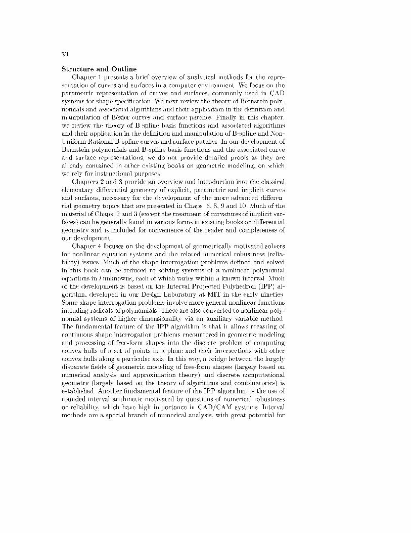
Structure and OutlineChapter 1 presents a brief overview of analytical methods for the repre-
sentation of curves and surfaces in a computer environment. We focus on theparametric representation of curves and surfaces, commonly used in CADsystems for shape speci�cation. We next review the theory of Bernstein poly-nomials and associated algorithms and their application in the de�nition andmanipulation of B�ezier curves and surface patches. Finally in this chapter,we review the theory of B-spline basis functions and associated algorithmsand their application in the de�nition and manipulation of B-spline and Non-Uniform Rational B-spline curves and surface patches. In our development ofBernstein polynomials and B-spline basis functions and the associated curveand surface representations, we do not provide detailed proofs as they arealready contained in other existing books on geometric modeling, on whichwe rely for instructional purposes.
Chapters 2 and 3 provide an overview and introduction into the classicalelementary di�erential geometry of explicit, parametric and implicit curvesand surfaces, necessary for the development of the more advanced di�eren-tial geometry topics that are presented in Chaps. 6, 8, 9 and 10. Much of thematerial of Chaps. 2 and 3 (except the treatment of curvatures of implicit sur-faces) can be generally found in various forms in existing books on di�erentialgeometry and is included for convenience of the reader and completeness ofour development.
Chapter 4 focuses on the development of geometrically motivated solversfor nonlinear equation systems and the related numerical robustness (relia-bility) issues. Much of the shape interrogation problems de�ned and solvedin this book can be reduced to solving systems of n nonlinear polynomialequations in l unknowns, each of which varies within a known interval. Muchof the development is based on the Interval Projected Polyhedron (IPP) al-gorithm, developed in our Design Laboratory at MIT in the early nineties.Some shape interrogation problems involve more general nonlinear functionsincluding radicals of polynomials. These are also converted to nonlinear poly-nomial systems of higher dimensionality via an auxiliary variable method.The fundamental feature of the IPP algorithm is that it allows recasting ofcontinuous shape interrogation problems encountered in geometric modelingand processing of free-form shapes into the discrete problem of computingconvex hulls of a set of points in a plane and their intersections with otherconvex hulls along a particular axis. In this way, a bridge between the largelydisparate �elds of geometric modeling of free-form shapes (largely based onnumerical analysis and approximation theory) and discrete computationalgeometry (largely based on the theory of algorithms and combinatorics) isestablished. Another fundamental feature of the IPP algorithm, is the use ofrounded interval arithmetic motivated by questions of numerical robustnessor reliability, which have high importance in CAD/CAM systems. Intervalmethods are a special branch of numerical analysis, with great potential for
VII
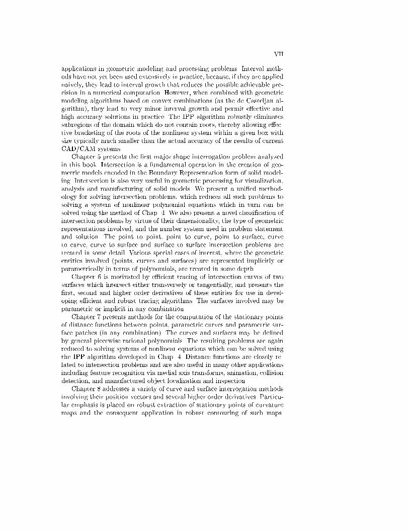
applications in geometric modeling and processing problems. Interval meth-ods have not yet been used extensively in practice, because, if they are appliednaively, they lead to interval growth that reduces the possible achievable pre-cision in a numerical computation. However, when combined with geometricmodeling algorithms based on convex combinations (as the de Casteljau al-gorithm), they lead to very minor interval growth and permit e�ective andhigh accuracy solutions in practice. The IPP algorithm robustly eliminatessubregions of the domain which do not contain roots, thereby allowing e�ec-tive bracketing of the roots of the nonlinear system within a given box withsize typically much smaller than the actual accuracy of the results of currentCAD/CAM systems.
Chapter 5 presents the �rst major shape interrogation problem analyzedin this book. Intersection is a fundamental operation in the creation of geo-metric models encoded in the Boundary Representation form of solid model-ing. Intersection is also very useful in geometric processing for visualization,analysis and manufacturing of solid models. We present a uni�ed method-ology for solving intersection problems, which reduces all such problems tosolving a system of nonlinear polynomial equations which in turn can besolved using the method of Chap. 4. We also present a novel classi�cation ofintersection problems by virtue of their dimensionality, the type of geometricrepresentations involved, and the number system used in problem statementand solution. The point to point, point to curve, point to surface, curveto curve, curve to surface and surface to surface intersection problems aretreated in some detail. Various special cases of interest, where the geometricentities involved (points, curves and surfaces) are represented implicitly orparametrically in terms of polynomials, are treated in some depth.
Chapter 6 is motivated by e�cient tracing of intersection curves of twosurfaces which intersect either transversely or tangentially, and presents the�rst, second and higher order derivatives of these entities for use in devel-oping e�cient and robust tracing algorithms. The surfaces involved may beparametric or implicit in any combination.
Chapter 7 presents methods for the computation of the stationary pointsof distance functions between points, parametric curves and parametric sur-face patches (in any combination). The curves and surfaces may be de�nedby general piecewise rational polynomials. The resulting problems are againreduced to solving systems of nonlinear equations which can be solved usingthe IPP algorithm developed in Chap. 4. Distance functions are closely re-lated to intersection problems and are also useful in many other applicationsincluding feature recognition via medial axis transforms, animation, collisiondetection, and manufactured object localization and inspection.
Chapter 8 addresses a variety of curve and surface interrogation methodsinvolving their position vectors and several higher order derivatives. Particu-lar emphasis is placed on robust extraction of stationary points of curvaturemaps and the consequent application in robust contouring of such maps.
VIII
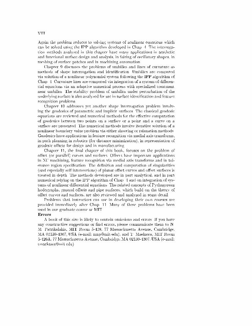
Again the problem reduces to solving systems of nonlinear equations whichcan be solved using the IPP algorithm developed in Chap. 4. The interroga-tion methods analyzed in this chapter have many applications in aestheticand functional surface design and analysis, in fairing of oscillatory shapes, inmeshing of surface patches and in machining automation.
Chapter 9 discusses the problems of umbilics and lines of curvature asmethods of shape interrogation and identi�cation. Umbilics are computedvia solution of a nonlinear polynomial system following the IPP algorithm ofChap. 4. Curvature lines are computed via integration of a system of di�eren-tial equations via an adaptive numerical process with specialized treatmentnear umbilics. The stability problem of umbilics under perturbation of theunderlying surface is also analyzed for use in surface identi�cation and featurerecognition problems.
Chapter 10 addresses yet another shape interrogation problem involv-ing the geodesics of parametric and implicit surfaces. The classical geodesicequations are reviewed and numerical methods for the e�ective computationof geodesics between two points on a surface or a point and a curve on asurface are presented. The numerical methods involve iterative solution of anonlinear boundary value problem via either shooting or relaxation methods.Geodesics have applications in feature recognition via medial axis transforms,in path planning in robotics (for distance minimization), in representation ofgeodesic o�sets for design and in manufacturing.
Chapter 11, the �nal chapter of this book, focuses on the problem ofo�set (or parallel) curves and surfaces. O�sets have important applicationsin NC machining, feature recognition via medial axis transforms and in tol-erance region speci�cation. The de�nition and computation of singularities(and especially self-intersections) of planar o�set curves and o�set surfaces istreated in depth. The methods developed are in part analytical, and in partnumerical relying on the IPP algorithm of Chap. 4 and on integration of sys-tems of nonlinear di�erential equations. The related concepts of Pythagoreanhodographs, general o�sets and pipe surfaces, which build on the theory ofo�set curves and surfaces, are also reviewed and analyzed in some detail.
Problems that instructors can use in developing their own courses areprovided immediately after Chap. 11. Many of these problems have beenused in our graduate course at MIT.Errors
A book of this size is likely to contain omissions and errors. If you haveany constructive suggestions or �nd errors, please communicate them to N.M. Patrikalakis, MIT Room 5-428, 77 Massachusetts Avenue, Cambridge,MA 02139-4307, USA (e-mail: [email protected]), and T. Maekawa, MIT Room5-426A, 77 Massachusetts Avenue, Cambridge, MA 02139-4307, USA (e-mail:[email protected]).

IX
AcknowledgementsWe wish to recognize the following former and current students who have
helped in the development of this book: Panos G. Alourdas, Christian Bliek,Julie S. Chalfant, Wonjoon Cho, Donald G. Danmeier, H. Nebi Gursoy, An-dreas Hofman, Chun-Yi Hu, Todd R. Jackson, Kwang Hee Ko, George A.Kriezis, Hongye Liu, John G. Nace, P. V. Prakash, Guoling Shen, Evan C.Sherbrooke, Stephen Smyth, Krishnan Sriram, Seamus T. Tuohy, Marsette A.Vona, Guoxin Yu and Jingfang Zhou. We also wish to acknowledge StephenL. Abrams for his assistance with software development and Fred Baker foreditorial assistance.
We also thank Chryssostomos Chryssostomidis, David C. Gossard, Mal-colm Sabin, Takis Sakkalis, Nickolas S. Sapidis, Franz-Erich Wolter and XiuziYe and several anonymous referees selected by Springer for useful discussionsand their comments.
We also wish to acknowledge MIT's funding of this book developmentfrom the Bernard M. Gordon Engineering Curriculum Development Fundvia the Dean of the School of Engineering and via additional support fromthe Department of Ocean Engineering.
We, �nally, dedicate this book to our families, our wives Sandra Jeanand Yuko and our children Alexander, Andrew, Nikki, and Takuya, whoselove, patience, understanding and encouragement made this lengthy projectpossible.
Cambridge, MA, June, 2001 Nicholas M. PatrikalakisTakashi Maekawa


Contents
1. Representation of Curves and Surfaces : : : : : : : : : : : : : : : : : : : 11.1 Analytic representation of curves . . . . . . . . . . . . . . . . . . . . . . . . . 1
1.1.1 Plane curves . . . . . . . . . . . . . . . . . . . . . . . . . . . . . . . . . . . . . 11.1.2 Space curves . . . . . . . . . . . . . . . . . . . . . . . . . . . . . . . . . . . . . 3
1.2 Analytic representation of surfaces . . . . . . . . . . . . . . . . . . . . . . . . 41.3 B�ezier curves and surfaces . . . . . . . . . . . . . . . . . . . . . . . . . . . . . . . 6
1.3.1 Bernstein polynomials . . . . . . . . . . . . . . . . . . . . . . . . . . . . 61.3.2 Arithmetic operations of polynomials in Bernstein form 71.3.3 Numerical condition of polynomials in Bernstein form . 91.3.4 De�nition of B�ezier curve and its properties . . . . . . . . . 121.3.5 Algorithms for B�ezier curves . . . . . . . . . . . . . . . . . . . . . . . 131.3.6 B�ezier surfaces . . . . . . . . . . . . . . . . . . . . . . . . . . . . . . . . . . . 18
1.4 B-spline curves and surfaces . . . . . . . . . . . . . . . . . . . . . . . . . . . . . 201.4.1 B-splines . . . . . . . . . . . . . . . . . . . . . . . . . . . . . . . . . . . . . . . . 201.4.2 B-spline curve . . . . . . . . . . . . . . . . . . . . . . . . . . . . . . . . . . . 211.4.3 Algorithms for B-spline curves . . . . . . . . . . . . . . . . . . . . . 241.4.4 B-spline surface . . . . . . . . . . . . . . . . . . . . . . . . . . . . . . . . . . 29
1.5 Generalization of B-spline to NURBS . . . . . . . . . . . . . . . . . . . . . 30
2. Di�erential Geometry of Curves : : : : : : : : : : : : : : : : : : : : : : : : : : 352.1 Arc length and tangent vector . . . . . . . . . . . . . . . . . . . . . . . . . . . . 352.2 Principal normal and curvature . . . . . . . . . . . . . . . . . . . . . . . . . . 392.3 Binormal vector and torsion . . . . . . . . . . . . . . . . . . . . . . . . . . . . . 432.4 Frenet-Serret formulae . . . . . . . . . . . . . . . . . . . . . . . . . . . . . . . . . . 47
3. Di�erential Geometry of Surfaces : : : : : : : : : : : : : : : : : : : : : : : : : 493.1 Tangent plane and surface normal . . . . . . . . . . . . . . . . . . . . . . . 493.2 First fundamental form I (metric) . . . . . . . . . . . . . . . . . . . . . . . . 523.3 Second fundamental form II (curvature) . . . . . . . . . . . . . . . . . . 553.4 Principal curvatures . . . . . . . . . . . . . . . . . . . . . . . . . . . . . . . . . . . . 593.5 Gaussian and mean curvatures . . . . . . . . . . . . . . . . . . . . . . . . . . . 64
3.5.1 Explicit surfaces . . . . . . . . . . . . . . . . . . . . . . . . . . . . . . . . . . 643.5.2 Implicit surfaces . . . . . . . . . . . . . . . . . . . . . . . . . . . . . . . . . . 65
3.6 Euler's theorem and Dupin's indicatrix . . . . . . . . . . . . . . . . . . . . 68

XII Contents
4. Nonlinear Polynomial Solvers and Robustness Issues : : : : : 734.1 Introduction . . . . . . . . . . . . . . . . . . . . . . . . . . . . . . . . . . . . . . . . . . . 734.2 Local solution methods . . . . . . . . . . . . . . . . . . . . . . . . . . . . . . . . . . 744.3 Classi�cation of global solution methods . . . . . . . . . . . . . . . . . . . 76
4.3.1 Algebraic and Hybrid Techniques . . . . . . . . . . . . . . . . . . . 764.3.2 Homotopy (Continuation) Methods . . . . . . . . . . . . . . . . . 784.3.3 Subdivision Methods . . . . . . . . . . . . . . . . . . . . . . . . . . . . . . 78
4.4 Projected Polyhedron algorithm . . . . . . . . . . . . . . . . . . . . . . . . . . 784.5 Auxiliary variable method for nonlinear systems with square
roots of polynomials . . . . . . . . . . . . . . . . . . . . . . . . . . . . . . . . . . . . 884.6 Robustness issues . . . . . . . . . . . . . . . . . . . . . . . . . . . . . . . . . . . . . . . 904.7 Interval arithmetic . . . . . . . . . . . . . . . . . . . . . . . . . . . . . . . . . . . . . . 924.8 Rounded interval arithmetic and its implementation . . . . . . . . 95
4.8.1 Double precision oating point arithmetic . . . . . . . . . . . 954.8.2 Extracting the exponent from the binary representation 984.8.3 Comparison of two di�erent unit�in�the�last�place
implementations . . . . . . . . . . . . . . . . . . . . . . . . . . . . . . . . . 1014.8.4 Hardware rounding for rounded interval arithmetic . . . 1024.8.5 Implementation of rounded interval arithmetic . . . . . . . 103
4.9 Interval Projected Polyhedron algorithm . . . . . . . . . . . . . . . . . . 1054.9.1 Formulation of the governing polynomial equations . . . 1054.9.2 Comparison of software and hardware rounding . . . . . . 106
5. Intersection Problems : : : : : : : : : : : : : : : : : : : : : : : : : : : : : : : : : : : : 1115.1 Overview of intersection problems . . . . . . . . . . . . . . . . . . . . . . . . 1115.2 Intersection problem classi�cation . . . . . . . . . . . . . . . . . . . . . . . . 113
5.2.1 Classi�cation by dimension . . . . . . . . . . . . . . . . . . . . . . . . 1145.2.2 Classi�cation by type of geometry . . . . . . . . . . . . . . . . . . 1145.2.3 Classi�cation by number system . . . . . . . . . . . . . . . . . . . . 116
5.3 Point/point intersection . . . . . . . . . . . . . . . . . . . . . . . . . . . . . . . . . 1165.4 Point/curve intersection . . . . . . . . . . . . . . . . . . . . . . . . . . . . . . . . . 116
5.4.1 Point/implicit algebraic curve intersection . . . . . . . . . . 1165.4.2 Point/rational polynomial parametric curve intersection1195.4.3 Point/procedural parametric curve intersection . . . . . . . 123
5.5 Point/surface intersection . . . . . . . . . . . . . . . . . . . . . . . . . . . . . . . 1235.5.1 Point/implicit algebraic surface intersection . . . . . . . . . . 1235.5.2 Point/rational polynomial parametric surface intersec-
tion . . . . . . . . . . . . . . . . . . . . . . . . . . . . . . . . . . . . . . . . . . . . 1245.5.3 Point/procedural parametric surface intersection . . . . . 127
5.6 Curve/curve intersection . . . . . . . . . . . . . . . . . . . . . . . . . . . . . . . . 1285.6.1 Rational polynomial parametric/implicit algebraic curve
intersection (Case D3) . . . . . . . . . . . . . . . . . . . . . . . . . . . . 1285.6.2 Rational polynomial parametric/rational polynomial
parametric curve intersection (Case D1) . . . . . . . . . . . . . 132

Contents XIII
5.6.3 Rational polynomial parametric/procedural paramet-ric and procedural parametric/procedural parametriccurve intersections (Cases D2 and D5) . . . . . . . . . . . . . . 133
5.6.4 Procedural parametric/implicit algebraic curve inter-section (Case D6) . . . . . . . . . . . . . . . . . . . . . . . . . . . . . . . . 135
5.6.5 Implicit algebraic/implicit algebraic curve intersection(Case D8) . . . . . . . . . . . . . . . . . . . . . . . . . . . . . . . . . . . . . . . 135
5.7 Curve/surface intersection . . . . . . . . . . . . . . . . . . . . . . . . . . . . . . . 1365.7.1 Rational polynomial parametric curve/implicit alge-
braic surface intersection (Case E3) . . . . . . . . . . . . . . . . . 1375.7.2 Rational polynomial parametric curve/rational poly-
nomial parametric surface intersection (Case E1) . . . . . 1375.7.3 Rational polynomial parametric/procedural paramet-
ric and procedural parametric/procedural parametriccurve/surface intersections (Cases E2/E6) . . . . . . . . . . . 138
5.7.4 Procedural parametric curve/implicit algebraic sur-face intersection (Case E7) . . . . . . . . . . . . . . . . . . . . . . . . 138
5.7.5 Implicit algebraic curve/implicit algebraic surface in-tersection (Case E11) . . . . . . . . . . . . . . . . . . . . . . . . . . . . . 139
5.7.6 Implicit algebraic curve/rational polynomial paramet-ric surface intersection (Case E9) . . . . . . . . . . . . . . . . . . . 139
5.8 Surface/surface intersections . . . . . . . . . . . . . . . . . . . . . . . . . . . . . 1395.8.1 Rational polynomial parametric/implicit algebraic sur-
face intersection (Case F3) . . . . . . . . . . . . . . . . . . . . . . . . 1405.8.2 Rational polynomial parametric/rational polynomial
parametric surface intersection (Case F1) . . . . . . . . . . . . 1495.8.3 Implicit algebraic/implicit algebraic surface intersec-
tion (Case F8) . . . . . . . . . . . . . . . . . . . . . . . . . . . . . . . . . . . 1535.9 Overlapping of curves and surfaces . . . . . . . . . . . . . . . . . . . . . . . . 1575.10 Self-intersection of curves and surfaces . . . . . . . . . . . . . . . . . . . . 1595.11 Summary . . . . . . . . . . . . . . . . . . . . . . . . . . . . . . . . . . . . . . . . . . . . . . 161
6. Di�erential Geometry of Intersection Curves : : : : : : : : : : : : : 1636.1 Introduction . . . . . . . . . . . . . . . . . . . . . . . . . . . . . . . . . . . . . . . . . . . 1636.2 More di�erential geometry of curves . . . . . . . . . . . . . . . . . . . . . . 1646.3 Transversal intersection curve . . . . . . . . . . . . . . . . . . . . . . . . . . . . 166
6.3.1 Tangential direction . . . . . . . . . . . . . . . . . . . . . . . . . . . . . . 1666.3.2 Curvature and curvature vector . . . . . . . . . . . . . . . . . . . . 1676.3.3 Torsion and third order derivative vector . . . . . . . . . . . . 1696.3.4 Higher order derivative vector . . . . . . . . . . . . . . . . . . . . . . 170
6.4 Intersection curve at tangential intersection points . . . . . . . . . . 1726.4.1 Tangential direction . . . . . . . . . . . . . . . . . . . . . . . . . . . . . . 1736.4.2 Curvature and curvature vector . . . . . . . . . . . . . . . . . . . . 1756.4.3 Third and higher order derivative vector . . . . . . . . . . . . 178
6.5 Examples . . . . . . . . . . . . . . . . . . . . . . . . . . . . . . . . . . . . . . . . . . . . . . 179

XIV Contents
6.5.1 Transversal intersection of parametric-implicit surfaces 1796.5.2 Tangential intersection of implicit-implicit surfaces . . . 181
7. Distance Functions : : : : : : : : : : : : : : : : : : : : : : : : : : : : : : : : : : : : : : : 1837.1 Introduction . . . . . . . . . . . . . . . . . . . . . . . . . . . . . . . . . . . . . . . . . . . 1837.2 Problem formulation . . . . . . . . . . . . . . . . . . . . . . . . . . . . . . . . . . . 184
7.2.1 De�nition of the distances between two point sets . . . . 1847.2.2 Geometric interpretation of stationarity of distance
function . . . . . . . . . . . . . . . . . . . . . . . . . . . . . . . . . . . . . . . . . 1867.3 More about stationary points . . . . . . . . . . . . . . . . . . . . . . . . . . . . 187
7.3.1 Classi�cation of stationary points . . . . . . . . . . . . . . . . . . . 1877.3.2 Nonisolated stationary points . . . . . . . . . . . . . . . . . . . . . . 192
7.4 Examples . . . . . . . . . . . . . . . . . . . . . . . . . . . . . . . . . . . . . . . . . . . . . . 194
8. Curve and Surface Interrogation : : : : : : : : : : : : : : : : : : : : : : : : : : 1978.1 Classi�cation of interrogation methods . . . . . . . . . . . . . . . . . . . . 197
8.1.1 Zeroth-order interrogation methods . . . . . . . . . . . . . . . . . 1988.1.2 First-order interrogation methods . . . . . . . . . . . . . . . . . . 1998.1.3 Second-order interrogation methods . . . . . . . . . . . . . . . . . 2028.1.4 Third-order interrogation methods . . . . . . . . . . . . . . . . . . 2078.1.5 Fourth-order interrogation methods . . . . . . . . . . . . . . . . . 210
8.2 Stationary points of curvature of free-form parametric surfaces2128.2.1 Gaussian curvature . . . . . . . . . . . . . . . . . . . . . . . . . . . . . . . 2128.2.2 Mean curvature . . . . . . . . . . . . . . . . . . . . . . . . . . . . . . . . . . 2158.2.3 Principal curvatures . . . . . . . . . . . . . . . . . . . . . . . . . . . . . . 216
8.3 Stationary points of curvature of explicit surfaces . . . . . . . . . . . 2178.4 Stationary points of curvature of implicit surfaces . . . . . . . . . . 2238.5 Contouring constant curvature . . . . . . . . . . . . . . . . . . . . . . . . . . . 225
8.5.1 Contouring levels . . . . . . . . . . . . . . . . . . . . . . . . . . . . . . . . . 2258.5.2 Finding starting points . . . . . . . . . . . . . . . . . . . . . . . . . . . . 2258.5.3 Mathematical formulation of contouring . . . . . . . . . . . . . 2278.5.4 Examples . . . . . . . . . . . . . . . . . . . . . . . . . . . . . . . . . . . . . . . 229
9. Umbilics and Lines of Curvature : : : : : : : : : : : : : : : : : : : : : : : : : : 2339.1 Introduction . . . . . . . . . . . . . . . . . . . . . . . . . . . . . . . . . . . . . . . . . . . 2339.2 Lines of curvature near umbilics . . . . . . . . . . . . . . . . . . . . . . . . . . 2349.3 Conversion to Monge form . . . . . . . . . . . . . . . . . . . . . . . . . . . . . . . 2399.4 Integration of lines of curvature . . . . . . . . . . . . . . . . . . . . . . . . . . 2449.5 Local extrema of principal curvatures at umbilics . . . . . . . . . . . 2469.6 Perturbation of generic umbilics . . . . . . . . . . . . . . . . . . . . . . . . . . 2529.7 In ection lines of developable surfaces . . . . . . . . . . . . . . . . . . . . . 258
9.7.1 Di�erential geometry of developable surfaces . . . . . . . . . 2589.7.2 Lines of curvature near in ection lines . . . . . . . . . . . . . . 264
Contents XV
10. Geodesics : : : : : : : : : : : : : : : : : : : : : : : : : : : : : : : : : : : : : : : : : : : : : : : : : 26710.1 Introduction . . . . . . . . . . . . . . . . . . . . . . . . . . . . . . . . . . . . . . . . . . . 26710.2 Geodesic equation . . . . . . . . . . . . . . . . . . . . . . . . . . . . . . . . . . . . . . 268
10.2.1 Parametric surfaces . . . . . . . . . . . . . . . . . . . . . . . . . . . . . . . 26810.2.2 Implicit surfaces . . . . . . . . . . . . . . . . . . . . . . . . . . . . . . . . . . 272
10.3 Two point boundary value problem . . . . . . . . . . . . . . . . . . . . . . . 27410.3.1 Introduction . . . . . . . . . . . . . . . . . . . . . . . . . . . . . . . . . . . . . 27410.3.2 Shooting method . . . . . . . . . . . . . . . . . . . . . . . . . . . . . . . . . 27510.3.3 Relaxation method . . . . . . . . . . . . . . . . . . . . . . . . . . . . . . . 276
10.4 Initial approximation . . . . . . . . . . . . . . . . . . . . . . . . . . . . . . . . . . . 27710.4.1 Linear approximation . . . . . . . . . . . . . . . . . . . . . . . . . . . . . 27710.4.2 Circular arc approximation . . . . . . . . . . . . . . . . . . . . . . . . 279
10.5 Shortest path between a point and a curve . . . . . . . . . . . . . . . . 28010.6 Numerical applications . . . . . . . . . . . . . . . . . . . . . . . . . . . . . . . . . . 283
10.6.1 Geodesic path between two points . . . . . . . . . . . . . . . . . . 28310.6.2 Geodesic path between a point and a curve . . . . . . . . . . 284
10.7 Geodesic o�sets . . . . . . . . . . . . . . . . . . . . . . . . . . . . . . . . . . . . . . . . 28610.8 Geodesics on developable surfaces . . . . . . . . . . . . . . . . . . . . . . . . 289
11. O�set Curves and Surfaces : : : : : : : : : : : : : : : : : : : : : : : : : : : : : : : 29511.1 Introduction . . . . . . . . . . . . . . . . . . . . . . . . . . . . . . . . . . . . . . . . . . . 295
11.1.1 Background and motivation . . . . . . . . . . . . . . . . . . . . . . . . 29511.1.2 NC machining . . . . . . . . . . . . . . . . . . . . . . . . . . . . . . . . . . . 29511.1.3 Medial axis . . . . . . . . . . . . . . . . . . . . . . . . . . . . . . . . . . . . . . 30111.1.4 Tolerance region . . . . . . . . . . . . . . . . . . . . . . . . . . . . . . . . . 308
11.2 Planar o�set curves . . . . . . . . . . . . . . . . . . . . . . . . . . . . . . . . . . . . . 30911.2.1 Di�erential geometry . . . . . . . . . . . . . . . . . . . . . . . . . . . . . 30911.2.2 Classi�cation of singularities . . . . . . . . . . . . . . . . . . . . . . . 31011.2.3 Computation of singularities . . . . . . . . . . . . . . . . . . . . . . . 31311.2.4 Approximations . . . . . . . . . . . . . . . . . . . . . . . . . . . . . . . . . . 314
11.3 O�set surfaces . . . . . . . . . . . . . . . . . . . . . . . . . . . . . . . . . . . . . . . . . 31811.3.1 Di�erential geometry . . . . . . . . . . . . . . . . . . . . . . . . . . . . . 31811.3.2 Singularities of o�set surfaces . . . . . . . . . . . . . . . . . . . . . . 32011.3.3 Self-intersection of o�sets of implicit quadratic surfaces 32111.3.4 Self-intersection of o�sets of explicit quadratic surfaces 33011.3.5 Self-intersection of o�sets of polynomial parametric
surface patches . . . . . . . . . . . . . . . . . . . . . . . . . . . . . . . . . . . 33711.3.6 Tracing of self-intersection curves . . . . . . . . . . . . . . . . . . . 34511.3.7 Approximations . . . . . . . . . . . . . . . . . . . . . . . . . . . . . . . . . . 347
11.4 Pythagorean hodograph . . . . . . . . . . . . . . . . . . . . . . . . . . . . . . . . . 35111.4.1 Curves . . . . . . . . . . . . . . . . . . . . . . . . . . . . . . . . . . . . . . . . . . 35111.4.2 Surfaces . . . . . . . . . . . . . . . . . . . . . . . . . . . . . . . . . . . . . . . . . 353
11.5 General o�sets . . . . . . . . . . . . . . . . . . . . . . . . . . . . . . . . . . . . . . . . . 35411.6 Pipe surfaces . . . . . . . . . . . . . . . . . . . . . . . . . . . . . . . . . . . . . . . . . . 355
11.6.1 Introduction . . . . . . . . . . . . . . . . . . . . . . . . . . . . . . . . . . . . . 355

XVI Contents
11.6.2 Local self-intersection of pipe surfaces . . . . . . . . . . . . . . . 35711.6.3 Global self-intersection of pipe surfaces . . . . . . . . . . . . . . 358
Problems : : : : : : : : : : : : : : : : : : : : : : : : : : : : : : : : : : : : : : : : : : : : : : : : : : : : : 369
A. Color Plates : : : : : : : : : : : : : : : : : : : : : : : : : : : : : : : : : : : : : : : : : : : : : : 379
References : : : : : : : : : : : : : : : : : : : : : : : : : : : : : : : : : : : : : : : : : : : : : : : : : : : : 383
Index : : : : : : : : : : : : : : : : : : : : : : : : : : : : : : : : : : : : : : : : : : : : : : : : : : : : : : : : : 407

1. Representation of Curves and Surfaces
We �rst introduce three forms to represent geometric objects mathematically.They are the parametric, implicit and explicit forms. Implicit and explicitforms are often referred to as nonparametric forms. Then we brie y reviewthe representation of curves and surfaces in B�ezier and B-spline form andtreat the special properties associated with each.
1.1 Analytic representation of curves
1.1.1 Plane curves
A plane curve can be expressed in the parametric form as
x = x(t); y = y(t) ; (1.1)
where the coordinates of the point (x; y) of the curve are expressed as func-tions of a parameter t within a closed interval t1 � t � t2. The functions x(t)and y(t) are assumed to be continuous with a su�cient number of continuousderivatives. The parametric curve is said to be of class r, if the functions havecontinuous derivatives up to the order r, inclusively [205]. In vector notationthe parametric curve can be speci�ed by a vector-valued function
r = r(t) : (1.2)
Another method of representing a curve analytically is to impose onecondition on a variable point (x; y) by an equation of the form
f(x; y) = 0 : (1.3)
This is an implicit equation for a plane curve. When f(x; y) is linear invariables x and y, (1.3) represents a straight line. If f(x; y) is of the seconddegree in x and y (i.e. ax2+2bxy+ cy2+2dx+2ey+h = 0), (1.3) representsa variety of plane curves called conic sections [79]. The implicit equationfor a plane curve can also be expressed as an intersection curve between aparametric surface and a plane. We will discuss this formulation in Chap. 5.

2 1. Representation of Curves and Surfaces
The explicit form can be considered as a special case of parametric andimplicit forms. If t can be expressed as a function of x or y, we can easilyeliminate t from (1.1) to generate the explicit form
y = F (x) or x = G(y) : (1.4)
This is always possible at least locally when dxdt 6= 0 or dy
dt 6= 0 [411]. Con-versely if we set x or y in (1.4) to be equal to the parameter t we obtainthe parametric form (1.1). Also if the implicit equation (1.3) can be solvedfor one variable in terms of the other, we also obtain (1.4). This is alwayspossible at least locally when @f
@y 6= 0 or @f@x 6= 0 [166].
−3 −2 −1 0 1 2 3
−2
−1.5
−1
−0.5
0
0.5
1
1.5
2
x
y
Fig. 1.1. Folium of Descartes
Example 1.1.1. Figure 1.1 shows the Folium of Descartes, introduced by R.Descartes in 1638, with its asymptotic line [226]. It can be expressed in para-metric form
r(t) =
�3t
1 + t3;
3t2
1 + t3
�T; �1 < t <1 (t 6= �1) ; (1.5)
where superscript T denotes transpose of a vector. For t < �1 the curve islocated in the fourth quadrant and approaches the origin as t goes to �1. For�1 < t < 0 the curve is located in the second quadrant, and t = 0 correspondsto the origin. In the �rst quadrant it forms a loop moving counter-clockwiseas t increases from 0 to +1. Eliminating t from (1.5), the Folium of Decartescan be also expressed in an implicit form
f(x; y) = x3 + y3 � 3xy = 0 : (1.6)
1.1 Analytic representation of curves 3
We can easily trace the curve using the parametric equation (1.5) by evalu-ating x(t) and y(t) for a discrete sampling of t, while such tracing is moredi�cult when using the implicit equation (1.6). However, determining if apoint (x0; y0) lies on the curve is easier when using the implicit rather thanthe parametric equation of the curve. For example, we can verify that thepoint ( 32 ;
32 ) lies on the curve by substituting x = 3
2 and y = 32 into implicit
form and deducing that f( 32 ;32 ) = 0. However, it is more complex to deduce
this using the parametric form. We �rst set x(t) = 32 which yields a cubic
equation t3� 2t+1 = 0. The roots of the cubic equation are 1, �1�p52 . Then
we substitute each root into y(t) to see if it becomes equal to 32 . An alternate
way to do this involves the theory of resultants from algebraic geometry thatwe will see in Sect. 5.4.2.
1.1.2 Space curves
The parametric representation of space curves is:
x = x(t); y = y(t); z = z(t); t1 � t � t2 : (1.7)
The implicit representation for a space curve can be expressed as an in-tersection curve between two implicit surfaces
f(x; y; z) = 0 \ g(x; y; z) = 0 ; (1.8)
or parametric and implicit surfaces
r = r(u; v) \ f(x; y; z) = 0 ; (1.9)
or two parametric surfaces
r = p(�; t) \ r = q(u; v) : (1.10)
The di�erential geometry properties of the intersection curves between im-plicit surfaces are discussed in Sects. 2.2 and 2.3 as well as in Chap. 6 togetherwith the intersection curves between parametric and implicit, and two para-metric surfaces. In Sect. 5.8 algorithms for computing the intersections (1.8),(1.9) and (1.10) are discussed.
If t can be expressed as a function of x, y, or z, we can eliminate t fromthe parametric form (1.7) to generate the explicit form. Let us assume t is afunction of x, then we have
y = Y (x); z = Z(x) : (1.11)
This is always possible at least locally when dxdt 6= 0 [411]. Also if the two
implicit equations f(x; y; z) = 0 and g(x; y; z) = 0 can be solved for two ofthe variables in terms of the third, for example y and z in terms of x, weobtain the explicit form (1.11). This is always possible at least locally when@f@y
@g@z � @f
@z@g@y 6= 0 [411]. Therefore the explicit equation for the space curve
can be expressed as an intersection curve of two cylinders projecting the curveonto xy and xz planes.

4 1. Representation of Curves and Surfaces
1.2 Analytic representation of surfaces
Similar to the curve case there are mainly three ways to represent surfaces,namely parametric, implicit and explicit methods. In parametric representa-tion the coordinates of a point (x; y; z) of the surface patch are expressed asfunctions of the parameters u and v in a closed rectangle:
x = x(u; v); y = y(u; v); z = z(u; v); u1 � u � u2; v1 � v � v2 : (1.12)The functions x(u; v), y(u; v) and z(u; v) are continuous and possess a su�-cient number of continuous partial derivatives. The parametric surface is saidto be of class r, if the functions have continuous (partial) derivatives up tothe order r, inclusively. In case the class is not explicitly given, it is assumedthat the functions have in�nitely many derivatives. In vector notation theparametric surface can be speci�ed by a vector-valued function
r = r(u; v) : (1.13)
An implicit surface is de�ned as the locus of points whose coordinates(x; y; z) satisfy an equation of the form
f(x; y; z) = 0 : (1.14)
When (1.14) is linear in variables x, y and z, it represents a plane. If (1.14)is of second degree in the variables x, y, z, it represents quadrics [79]
ax2 + by2 + cz2 + dxy + eyz + hxz + kx+ ly +mz + n = 0 : (1.15)
Some of the quadric surfaces such as elliptic paraboloid, hyperbolic paraboloidand parabolic cylinder have explicit forms (see Fig. 8.9). Paraboloid of revo-lution is a special case of elliptic paraboloid where the major and minor axesare the same. The rest of the quadrics have implicit forms including ellip-soid, elliptic cone, elliptic cylinder, hyperbolic cylinder, hyperboloid of onesheet and two sheets, where the hyperboloid of revolution is a special form.The natural quadrics, sphere, circular cone and circular cylinder, which arespecial cases of ellipsoid, elliptic cone and elliptic cylinder, are widely usedin mechanical design and CAD/CAM systems. Also they result from stan-dard manufacturing operations such as rolling, turning, �lleting, drilling andmilling [149]. According to a survey conducted by the Production Automa-tion Project group at the University of Rochester in the mid 1970's, 80-85% ofmechanical parts were adequately represented by planes and cylinders, while90-95% were modeled with the addition of cones [433, 362, 149].
If the implicit equation (1.14) can be solved for one of the variables as afunction of the other two, say z is solved in terms of x and y, we obtain anexplicit surface
z = F (x; y) : (1.16)

1.2 Analytic representation of surfaces 5
This is always possible at least locally when @f@z 6= 0 [166]. And if the two
variables u, v of the parametric form can be solved in terms of x and y, wecan substitute u = u(x; y) and v = v(x; y) into z = z(u; v) which yields anexplicit form. This is possible when @x
@u@y@v � @x
@v@y@u 6= 0 [76]. Conversely when
the explicit form z = F (x; y) is given, the parametric form is derived bysetting x = u, y = v, z = F (u; v). Thus, the explicit form can be consideredas a special case of implicit and parametric forms.
Example 1.2.1. Let us consider a hyperbolic paraboloid surface patch in theparametric form:
x = u+ v; y = u� v; z = u2 � v2; 0 � u; v � 1 : (1.17)
Since we can easily solve for u and v in terms of x and y as u = x+y2 and
v = x�y2 , the explicit form is obtained as
z = xy; 0 � x+ y � 2; 0 � x� y � 2 : (1.18)
Table 1.1. Representations of curves and surfaces
Geometry Parametric Implicit Explicit
Plane x = x(t), y = y(t) f(x; y) = 0 or y = F (x)curves t1 � t � t2 r = r(u; v) \ plane
Space x = x(t), y = y(t), f(x; y; z) = 0 \ g(x; y; z) = 0 y = Y (x) \curves z = z(t), t1 � t � t2 or r = r(u; v) \ f(x; y; z) = 0 z = Z(x)
or r = p(�; t) \ r = q(u; v)
Surfaces x = x(u; v), f(x; y; z) = 0 z = F (x; y)y = y(u; v),z = z(u; v),u1 � u � u2,v1 � v � v2
Table 1.1 summarizes the three representation forms for plane curves,space curves and surfaces. Table 1.2 compares the three representations[119, 116]. It is clear from the tables that the parametric form is the mostversatile method among the three and the explicit is the least. Furthermore,the explicit form can always be easily converted to parametric form. There-fore we will mainly focus on the parametric and implicit forms throughoutthis book. Methods to �t and manipulate free-form shapes in implicit formare more complex than those for the parametric form both with respect tocomputation and geometric intuition. However, a considerable body of re-search aimed at alleviating precisely this obstacle has been published overthe last �fteen years, see for example [372, 298, 16]. In this book we do notcover implicit surface �tting and design methods.

6 1. Representation of Curves and Surfaces
Table 1.2. Comparison of di�erent methods of curve and surface representation
Disadvantages
Explicit Implicit Parametric
� In�nite slopes are im-possible if f(x) is a poly-nomial.
� Di�cult to �t andmanipulate free formshapes.
� High exibility compli-cates intersections andpoint classi�cation.
� Axis dependent (di�-cult to transform).
� Axis dependent.
� Closed and multival-ued curves are di�cult torepresent.
� Complex to trace.
Advantages
Explicit Implicit Parametric
� Easy to trace. � Closed and multival-ued curves and in�niteslopes can be repre-sented.
� Closed and multival-ued curves and in�niteslopes can be repre-sented.
� Point classi�cation(solid modeling, in-terference check) iseasy.
� Axis independent (easyto transform).
� Intersections/o�setscan be represented.
� Easy to generate com-posite curves.� Easy to trace.� Easy in �tting andmanipulating free-formshapes.
1.3 B�ezier curves and surfaces
Good introductory books on B�ezier/B-spline curves and surfaces are providedby Faux and Pratt [116], Mortenson [275], Ding and Davies [75], Rogers andAdams [347], Beach [21], Nowacki et al. [288] and Lee [230], while for a morecomprehensive mathematical introduction to B-splines, Bezier and B-splinecurves and surfaces, the reader should refer to textbooks by Yamaguchi [454],Hosaka [173], Risler [345], Farin [92], Hoschek and Lasser [175], Piegl andTiller [313] and Gallier [121].
1.3.1 Bernstein polynomials
The Bernstein polynomials are de�ned as
Bi;n(t) =n!
i!(n� i)! (1� t)n�iti; i = 0; : : : ; n : (1.19)

1.3 B�ezier curves and surfaces 7
They form a basis for polynomials (see Sect. 4.4) and have several propertiesof interest:
� Non-negativity: Bi;n(t) � 0; 0 � t � 1; i = 0; : : : ; n .� Partition of unity:
Pni=0Bi;n(t) = (1 � t + t)n = 1 (by the binomial
theorem).� Symmetry:
Bi;n(t) = Bn�i;n(1� t) : (1.20)
� Recursion: Bi;n(t) = (1� t)Bi;n�1(t) + tBi�1;n�1(t) with Bi;n(t) = 0 fori < 0, i > n and B0;0(t) = 1 .
� Linear precision:
t =
nXi=0
i
nBi;n(t) ; (1.21)
which implies that the monomial t can be expressed as the weighted sumof Bernstein polynomials of degree n with coe�cients evenly spaced in theinterval [0,1]. This property is used extensively in Chaps. 4 and 5.
� Degree elevation: The basis functions of degree n can be expressed interms of those of degree n+ 1 [106] as:
Bi;n(t) =
�1� i
n+ 1
�Bi;n+1(t) +
i+ 1
n+ 1Bi+1;n+1(t) ; (1.22)
where i = 0; 1; � � � ; n. Or more generally in terms of basis functions ofdegree n+ r [106] as:
Bi;n(t) =
i+rXj=i
�ni
��r
j � i�
�n+ rj
� Bj;n+r(t); i = 0; 1; � � � ; n : (1.23)
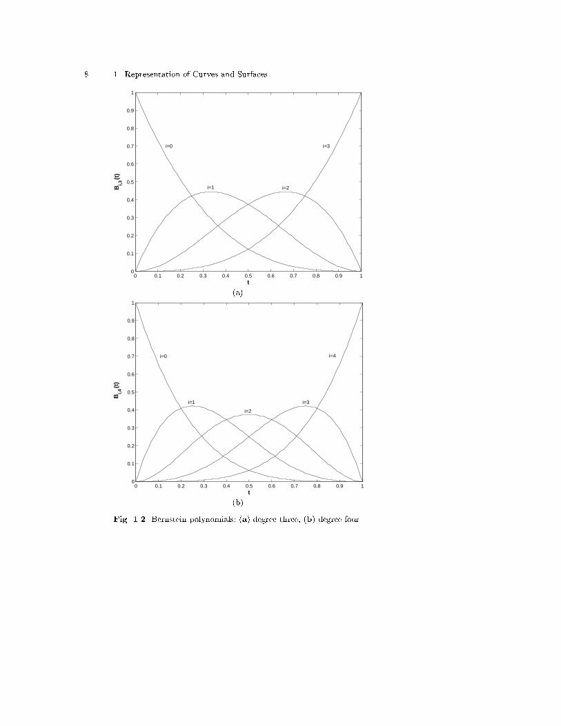
Figure 1.2 shows the Bernstein polynomials of degree 3 and 4. The deriva-tive of a Bernstein polynomial is
dBi;n(t)
dt= n[Bi�1;n�1(t)�Bi;n�1(t)] ; (1.24)
where B�1;n�1(t) = Bn;n�1(t) = 0.
1.3.2 Arithmetic operations of polynomials in Bernstein form
Arithmetic operations between polynomials are often required for shape inter-rogation (see for example Chaps. 4, 5, etc.). Farouki and Rajan [106] provide
8 1. Representation of Curves and Surfaces
0 0.1 0.2 0.3 0.4 0.5 0.6 0.7 0.8 0.9 10
0.1
0.2
0.3
0.4
0.5
0.6
0.7
0.8
0.9
1
t
Bi,3
(t)
i=0
i=1 i=2
i=3
(a)
0 0.1 0.2 0.3 0.4 0.5 0.6 0.7 0.8 0.9 10
0.1
0.2
0.3
0.4
0.5
0.6
0.7
0.8
0.9
1
t
Bi,4
(t)
i=0
i=1
i=2
i=3
i=4
(b)
Fig. 1.2. Bernstein polynomials: (a) degree three, (b) degree four

1.3 B�ezier curves and surfaces 9
formulae for such arithmetic operations of polynomials in Bernstein form.Let the two polynomials f(t) and g(t) of degree m and n with Bernsteincoe�cients fmi and gni be as follows:
f(t) =
mXi=0
fmi Bi;m(t); g(t) =
nXi=0
gni Bi;n(t); 0 � t � 1 : (1.25)
� Addition and subtractionIf the degrees of the two polynomials are the same, i.e. m = n, we simplyadd or subtract the coe�cients
f(t) + g(t) =
mXi=0
(fmi � gmi )Bi;m(t) : (1.26)
If m > n, we need to �rst degree elevate g(t) m�n times using (1.23) andthen add or subtract the coe�cients
f(t) + g(t) =
mXi=0
0BB@fmi �
min(n;i)Xj=max(0;i�m+n)
�nj
��m� ni� j
��mi
� gnj
1CCABi;m(t) :
(1.27)
� MultiplicationMultiplication of two polynomials of degree m and n yields a degree m+npolynomial
f(t)g(t) =m+nXi=0
0BB@
min(m;i)Xj=max(0;i�n)
�mj
��n
i� j�
�m+ ni
� fmj gni�j
1CCABi;m+n(t) :
(1.28)
1.3.3 Numerical condition of polynomials in Bernstein form
Polynomials in the Bernstein basis have better numerical stability under per-turbation of their coe�cients than in the power basis. We will introduce theconcept of condition numbers for polynomial roots investigated by Faroukiand Rajan [105].
Let us consider a polynomial f(t) in the basis �i(t) with coe�cients fi:
f(t) =nXi=0
fi�i(t) : (1.29)
If we perturb a single coe�cient fj by �fj , we have

10 1. Representation of Curves and Surfaces
~f(t) = f0�0(t) + f1�1(t) + : : :+ (fj + �fj)�j(t) + : : :+ fn�n(t) ; (1.30)
or using (1.29)
~f(t) = f(t) + �fj�j(t) : (1.31)
If t+ �t is a root of the perturbed polynomial ~f(t), then
~f(t+ �t) = f(t+ �t) + �fj�j(t+ �t) = 0 ; (1.32)
or
f(t+ �t) = ��fj�j(t+ �t) : (1.33)
Now let us Taylor expand (1.33) about t0, where t0 is a root of f(t), i.e.f(t0) = 0,
nXi=1
(�t)i
i!
dif
dti(t0) = ��fj
nXi=0
(�t)i
i!
di�jdti
(t0) : (1.34)
If t0 is a simple root of f(t), then _f(t0) 6= 0, and in the limit of in�nitesimalperturbations the above equation gives:
lim�fj!0
�t�fjfj
= �fj�j(to)_f(t0)
: (1.35)
The absolute value of the right hand side of the above equation
C = jfj�j(to)= _f(t0)j ; (1.36)
is called the condition number of the root t0 with respect to the single coe�-cient fj . For perturbations in each coe�cient, fj , j = 0; 1; : : : ; n, the conditionnumber of the root t0 becomes:
C =
Pnj=0 jfj�j(to)jj _f(t0)j
: (1.37)
If t0 is an m-fold root, m � 2, then a multiple-root condition numberC(m) for perturbations in each coe�cient fj , j = 0; 1; : : : ; n is de�ned as
C(m) =
0@ m!
jdmf(t0)dtm jnXj=0
jfj�j(t0)j1A1=m
: (1.38)
The following theorem is due to Farouki and Rajan [105].

1.3 B�ezier curves and surfaces 11
Table 1.3. Condition numbers for Wilkinson polynomial (adapted from [105])
i Cp(x0) Cb(x0)
1 2:100 � 101 3:413 � 100
2 4:389 � 103 1:453 � 102
3 3:028 � 105 2:335 � 103
4 1:030 � 107 2:030 � 104
5 2:059 � 108 1:111 � 105
6 2:667 � 109 4:153 � 105
7 2:409 � 1010 1:115 � 106
8 1:566 � 1011 2:215 � 106
9 7:570 � 1011 3:321 � 106
10 2:775 � 1012 3:797 � 106
11 7:822 � 1012 3:321 � 106
12 1:707 � 1013 2:215 � 106
13 2:888 � 1013 1:115 � 106
14 3:777 � 1013 4:153 � 105
15 3:777 � 1013 1:111 � 105
16 2:833 � 1013 2:030 � 104
17 1:541 � 1013 2:335 � 103
18 5:742 � 1012 1:453 � 102
19 1:310 � 1012 3:413 � 100
20 1:378 � 1011 0
Theorem 1.3.1. For an arbitrary polynomial f(t) with a simple root t0 2[0; 1], let Cp(t0) and Cb(t0) denote the condition numbers (1.37) of the rootin the power and Bernstein bases on [0; 1], respectively. Then Cb(t0) � Cp(t0)for all t0 2 [0; 1]. In particular Cb(0) = Cp(0) = 0, while for t0 2 (0; 1] wehave the strict inequality Cb(t0) < Cp(t0).
As an illustration of the above theorem, let us consider Wilkinson's poly-nomial in which twenty real roots are equally distributed on [0; 1]:
f(t) =
20Yi=1
(t� i=20) : (1.39)
The condition numbers for each root with respect to a perturbation in thesingle coe�cient of t19 are shown in Table 1.3 [105]. We can clearly observethat the condition numbers of the root in the Bernstein basis are severalorders of magnitude smaller than in the power basis. This serves to illustratethe attractiveness of using the Bernstein basis in computations in CAD/CAM

12 1. Representation of Curves and Surfaces
systems. Although not a panacea, Bernstein basis when used properly ina oating point environment increases reliability of computations (see alsodetailed discussions in Chaps. 4 and 5).
1.3.4 De�nition of B�ezier curve and its properties
A B�ezier curve is a parametric curve that uses the Bernstein polynomials asa basis. A B�ezier curve of degree n (order n+ 1) is represented by
r(t) =
nXi=0
biBi;n(t); 0 � t � 1 : (1.40)
The coe�cients, bi, are the control points or B�ezier points and together withthe basis function Bi;n(t) determine the shape of the curve. Lines drawnbetween consecutive control points of the curve form the control polygon. Acubic B�ezier curve together with its control polygon is shown in Fig. 1.3 (a).B�ezier curves have the following properties:
� Geometry invariance property: Partition of unity property of the Bern-stein polynomial assures the invariance of the shape of the B�ezier curveunder translation and rotation of its control points.
� End points geometric property:{ The �rst and last control points are the endpoints of the curve. In otherwords, b0 = r(0) and bn = r(1).
{ The curve is tangent to the control polygon at the endpoints. This canbe easily observed by taking the �rst derivative of a B�ezier curve
_r(t) =dr(t)
dt= n
n�1Xi=0
(bi+1 � bi)Bi;n�1(t); 0 � t � 1 : (1.41)
In particular we have _r(0) = n(b1 � b0) and _r(1) = n(bn � bn�1).Equation (1.41) can be simpli�ed by setting �bi = bi+1 � bi:
_r(t) = n
n�1Xi=0
�biBi;n�1(t); 0 � t � 1 : (1.42)
The �rst derivative of a B�ezier curve, which is called hodograph, is an-other B�ezier curve whose degree is lower than the original curve by oneand has control points n�bi, i = 0; � � � ; n� 1. Hodographs are useful inthe study of intersection (see Sect. 5.6.2) and other interrogation prob-lems such as singularities and in ection points.
� Convex hull property: A domain D is convex if for any two points P1 andP2 in the domain, the segment P1P2 is entirely contained in the domainD [334]. It can be shown that the intersection of convex domains is a

1.3 B�ezier curves and surfaces 13
convex domain. The convex hull of a set of points P is the boundary of thesmallest convex domain containing P . There are several e�cient algorithmsfor computing the convex hull of a set of points [334, 66, 291].Using the above de�nitions and facts, the convex hull of a B�ezier curveis the boundary of the intersection of all the convex sets containing allvertices or the intersection of the half spaces generated by taking threevertices at a time to construct a plane and having all other vertices onone side. The convex hull can also be conceptualized at the shape of arubber band in 2-D or a sheet in 3-D stretched taut over the polygonvertices [75]. The entire curve is contained within the convex hull of thecontrol points as shown in Fig. 1.3 (b). The convex hull property is useful inintersection problems (see Fig. 1.4), in detection of absence of interferenceand in providing estimates of the position of the curve through simple ande�ciently computable bounds.
� Variation diminishing property:{ 2-D: The number of intersections of a straight line with a planarB�ezier curve is no greater than the number of intersections of the linewith the control polygon. A line intersecting the convex hull of a planarB�ezier curve may intersect the curve transversally, be tangent to thecurve, or not intersect the curve at all. It may not, however, intersect thecurve more times than it intersects the control polygon. This propertyis illustrated in Fig. 1.5.
{ 3-D: The same relation holds true for a plane with a space B�eziercurve.
From this property, we can roughly say that a B�ezier curve oscillates lessthan its control polygon, or in other words, the control polygon's segmentsexaggerate the oscillation of the curve. This property is important in in-tersection algorithms and in detecting the fairness of B�ezier curves.
� Symmetry property: If we renumber the control points as b�n�i = bi, orin other words relabel from b0;b1; : : : ;bn to bn;bn�1; : : : ;b0 and usingthe symmetry property of the Bernstein polynomial (1.20) the followingidentity holds:
nXi=0
biBi;n(t) =
nXi=0
b�iBi;n(1� t) : (1.43)
1.3.5 Algorithms for B�ezier curves
� Evaluation and subdivision algorithm: A B�ezier curve can be evaluatedat a speci�c parameter value t0 and the curve can be split at that valueusing the de Casteljau algorithm [175], where the following equation
bki (t0) = (1� t0)bk�1i�1 + t0b
k�1i ; k = 1; 2; : : : ; n; i = k; : : : ; n ;
(1.44)

14 1. Representation of Curves and Surfaces
b0
b1
b2
b3
Control Polygon
(a)
b0
b1
b2
b3
Convex Hull
(b)
Fig. 1.3. A cubic B�ezier curve: (a) with control polygon, (b) with convex hull
is applied recursively to obtain the new control points. The algorithm isillustrated in Fig. 1.6, and has the following properties:{ The values b0i are the original control points of the curve.{ The value of the curve at parameter value t0 is b
nn.
{ The curve is split at parameter value to and can be represented as twocurves, with control points (b00, b
11,: : :, b
nn) and (bnn; b
n�1n ; : : : ; b0n).
� Continuity algorithm: B�ezier curves can represent complex curves byincreasing the degree and thus the number of control points. Alterna-tively, complex curves can be represented using composite curves, which

1.3 B�ezier curves and surfaces 15
Fig. 1.4. Comparison of convex hulls of B�ezier curves as means of detecting inter-section
Possible Impossible
Fig. 1.5. Variation diminishing property of a cubic B�ezier curve
can be formed by joining several B�ezier curves end to end. If this methodis adopted, the continuity between consecutive curves must be addressed.One set of continuity conditions are the geometric continuity conditions,designated by the letter G with an integer exponent. Position continuity,or G0 continuity, requires the endpoints of the two curves to coincide,
ra(1) = rb(0) : (1.45)
The superscripts denote the �rst and second curves. Tangent continuity, orG1 continuity, requires G0 continuity and in addition the tangents of thecurves to be in the same direction,
_ra(1) = �1t ; (1.46)
_rb(0) = �2t ; (1.47)
where t is the common unit tangent vector and �1, �2 are the magnitudeof _ra(1) and _rb(0). G1 continuity is important in minimizing stress con-centrations in physical solids loaded with external forces and in helpingprevent ow separation in uids.

16 1. Representation of Curves and Surfaces
b03 =b0
2 =b01 =b0
0
b10 b2
0
b30
t
1-t
t 1-t
t
1-tb1
3 =b12 =b1
1
b21
b31b2
2
b32
b33
b00
b10
b20
b30
b11
b21
b31
b22
b32
1−t
t
1−t
1−t
1−t
1−tt
t
t
t
b3=r(t)3
1−t
t
Fig. 1.6. The de Casteljau algorithm
Curvature continuity, or G2 continuity, requires G1 continuity and in ad-dition the center of curvature to move continuously past the connectionpoint [116],
�rb(0) =
��2�1
�2
�ra(1) + � _ra(1) ; (1.48)
1.3 B�ezier curves and surfaces 17
where � is an arbitrary constant. G2 continuity is important for aestheticreasons and also for helping prevent uid ow separation.More stringent continuity conditions are the parametric continuity con-ditions, where Ck continuity requires the kth derivative (and all lowerderivatives) of each curve to be equal at the joining point. In other words,
dkra(1)
dtk=dkrb(0)
dtk: (1.49)
Let us assume that the global parameter t, associated with the i-th segmentof a composite degree n B�ezier curve with local parameter ui (0 � ui � 1),runs over the interval [ti, ti+1]. Then the i-th segment of a composite B�eziercurve is given by:
ri(t) =
nXj=0
bni+jBj;n(ui) ; (1.50)
where the global parameter t and the local parameter ui are related by,
0 � ui = t� titi+1 � ti � 1 : (1.51)
If we denote hi = ti+1 � ti, the C1 and C2 continuity conditions for thei-th and i+1-th segments of the composite B�ezier curve can be statedas [454, 175]:
hi+1 (bni � bni�1) = hi (bni+1 � bni) ; (1.52)
and
bni�1 +hi+1
hi(bni�1 � bni�2) = bni+1 +
hihi+1
(bni+1 � bni+2) :
(1.53)
Figure 1.7 illustrates the connection of two cubic B�ezier curve segments att = ti+1.
� Degree elevation: The degree elevation algorithm permits us to increasethe degree of a B�ezier curve from n to n + 1 and the number of controlpoints from n + 1 to n + 2 without changing the shape of the curve. Thenew control points bn+1
i of the degree n+ 1 curve are given by
bn+1i =
i
n+ 1bni�1 +
�1� i
n+ 1
�bni ; i = 0; : : : ; n+ 1 ; (1.54)
where bn�1 = bnn+1 = 0. The degree elevation algorithm for a B�ezier curvefrom degree n to n+ r is given by [106]:
bn+ri =
min(n;i)Xj=max(0;i�r)
�nj
��r
i� j�
�n+ ri
� bnj ; i = 0; 1; � � � ; n+ r : (1.55)

18 1. Representation of Curves and Surfaces
bn i-3 bn i+3
bn i-2
bn i+2
bn i-1
bn i+1
bn ihi
::
hi+1
hi::
hi+1
hi::
hi+1
Fig. 1.7. Continuity conditions
1.3.6 B�ezier surfaces
A tensor product surface patch is formed by moving a curve through spacewhile allowing deformations in that curve. This can be thought of as allowingeach control point bi to sweep a curve in space. If this surface is representedusing Bernstein polynomials, a B�ezier surface patch is formed, with the fol-lowing formula:
r(u; v) =
mXi=0
nXj=0
bijBi;m(u)Bj;n(v); 0 � u; v � 1 : (1.56)
Here, the set of straight lines drawn between consecutive control points bij isreferred to as the control net. It is easy to see that boundary iso-parametriccurves (u = 0, u = 1, v = 0 and v = 1) have the same control points asthe corresponding boundary points on the net. An example of a bi-quadraticB�ezier surface with its control net can be seen in Fig. 1.8. Since a B�eziersurface is a direct extension of univariate B�ezier curve to its bivariate form,it inherits many of the properties of the B�ezier curve described in Sect. 1.3.4such as:
� Geometry invariance property.� End points geometric property.� Convex hull property.
However, no variation diminishing property is known for B�ezier surfacepatches.
The surface patches treated in this book are mostly topologically quadri-lateral. However we sometimes need to use topologically triangular patches. Insuch cases, we may collapse one boundary curve of a quadrilateral patch into

1.3 B�ezier curves and surfaces 19
a single point to form a three-sided patch as shown in Fig. 1.9. Such a trian-gular patch is said to be degenerate [116, 92]. Alternatively one could arrangefor two partial derivatives ru and rv at one of the corners of a quadrilateralpatch (1.56) to be collinear to create degenerate patches [92]. The di�erentialgeometry of degenerated patches is studied in [116, 452, 456].
b20 b21
b22
b10
b12b00
b01
b02
Fig. 1.8. A bi-quadratic B�ezier surface with control net
Fig. 1.9. Octant of ellipsoid, represented by a degenerate patch

20 1. Representation of Curves and Surfaces
1.4 B-spline curves and surfaces
The B�ezier representation has two main disadvantages. First, the number ofcontrol points is directly related to the degree. Therefore, to increase the com-plexity of the shape of the curve by adding control points requires increasingthe degree of the curve or satisfying the continuity conditions between con-secutive segments of a composite curve. Second, changing any control pointa�ects the entire curve or surface, making design of speci�c sections very di�-cult. These disadvantages are remedied with the introduction of the B-spline(basis-spline) representation.
Early fundamental work on the B-spline basis functions was performedalmost 50 years ago by Schoenberg [367], and this was followed by develop-ment of fundamental algorithms by Cox [67] and de Boor [72, 73]. B-splines inthe context of Computer Aided Geometric Design were proven to be a viableand attractive representation method by many pioneers of this �eld, suchas Riesenfeld [344, 130], Boehm [33], Schumaker [368] and many subsequentresearchers.
In this section, we provide de�nitions and the basic properties and algo-rithms of B-splines. However, we do not deal with �tting, approximation andfairing methods using B-splines which are very important in their own right.For these topics, there are specialized books, monographs and proceedingsand a large variety of papers [364, 175, 92, 313, 45].
1.4.1 B-splines
An order k B-spline is formed by joining several pieces of polynomials ofdegree k � 1 with at most Ck�2 continuity at the breakpoints. A set of non-descending breaking points t0 � t1 � : : : � tm de�nes a knot vector
T = (t0; t1; : : : ; tm) ; (1.57)
which determines the parametrization of the basis functions.Given a knot vector T, the associated B-spline basis functions, Ni;k(t),
are de�ned as:
Ni;1(t) =
�1 for ti � t < ti+1
0 otherwise ;(1.58)
for k = 1, and
Ni;k(t) =t� ti
ti+k�1 � tiNi;k�1(t) +ti+k � t
ti+k � ti+1Ni+1;k�1(t) ; (1.59)
for k > 1 and i = 0; 1; : : : ; n. These equations have the following proper-ties [175]:
� Positivity: Ni;k(t) > 0, for ti < t < ti+k.

1.4 B-spline curves and surfaces 21
� Local support: Ni;k(t) = 0, for t0 � t � ti, and ti+k � t � tn+k.� Partition of unity:
Pni=0Ni;k(t) = 1, for t 2 [t0; tm].
� Recursion: Given by (1.59).� Continuity: Ni;k(t) has C
k�2 continuity at each simple knot.
The concept of nodes orGreville abscissae [130, 92], which are the averagesof the knots, are important in B-spline approximations [130, 451] and de�nedas follows:
�i =1
k � 1(ti+1 + ti+2 + � � �+ ti+k�1) : (1.60)
The node �i generally lies near the parameter value which corresponds to amaximum of the basis function Ni;k(t) [344, 313].
The derivative of the B-spline basis function is given by [313]
dNi;k(t)
dt=
k � 1
ti+k�1 � tiNi;k�1(t)� k � 1
ti+k � ti+1Ni+1;k�1(t) : (1.61)
1.4.2 B-spline curve
A B-spline curve is de�ned as a linear combination of control points pi andB-spline basis functions Ni;k(t) given by
r(t) =nXi=0
piNi;k(t); n � k � 1; t 2 [tk�1; tn+1] : (1.62)
In this context the control points are called de Boor points. The basis functionNi;k(t) is de�ned on a knot vector
T = (t0; t1; : : : ; tk�1; tk; tk+1; : : : ; tn�1; tn; tn+1; : : : ; tn+k) ; (1.63)
where there are n+k+1 elements, i.e. the number of control points n+1 plusthe order of the curve k. Each knot span ti � t � ti+1 is mapped onto a poly-nomial curve between two successive joints r(ti) and r(ti+1). Normalizationof the knot vector, so it covers the interval [0,1], is helpful in improving nu-merical accuracy in oating point arithmetic computation due to the higherdensity of oating point numbers in this interval [133, 299].
A B-spline curve has the following properties:
� Geometry invariance property: Partition of unity property of the B-splineassures the invariance of the shape of the B-spline curve under translationand rotation.
� End points geometric property:{ Unlike B�ezier curves, B-spline curves do not in general pass through thetwo end control points. Increasing the multiplicity of a knot reduces thecontinuity of the curve at that knot. Speci�cally, the curve is (k� p� 1)

22 1. Representation of Curves and Surfaces
t
1
o
t1
t2
t3
t4 t7t8t9t10
t6t5
N0,4
N1,4 N2,4
N3,4 N4,4 N5,4
N6,4
N0,4 is C-1
N0,4 is C2 N1,4 is C
2
N5,4 is C2
N2,4 is C2
N6,4 is C0
N1,4 is C2
N4,4 is C2
N1,4 is C0
N2,4 is C1
N3,4 is C2
N3,4 is C2
N4,4 is C1
N5,4 is C0
N6,4 is C-1
Fig. 1.10. An order four B-spline basis functions with uniform knot vector
times continuously di�erentiable at a knot with multiplicity p (� k), andthus has C(k�p�1) continuity. Therefore, the control polygon will coincidewith the curve at a knot of multiplicity k�1, and a knot with multiplicityk indicates C�1 continuity, or a discontinuous curve. Repeating the knotsat the end k times will force the endpoints to coincide with the controlpolygon. Thus the �rst and the last control points of a curve with a knotvector described by
T = (t0; t1; : : : ; tk�1;| {z }k equal knots
tk; tk+1; : : : ; tn�1; tn;| {z }n-k+1 internal knots
tn+1; : : : ; tn+k| {z }k equal knots
) ; (1.64)
coincide with the endpoints of the curve. Such knot vectors and curvesare known as clamped [313]. In other words, clamped/unclamped refersto whether both ends of the knot vector have multiplicity equal to k ornot. Figure 1.10 shows cubic B-spline basis functions de�ned on a knotvector T = (t0 = t1 = t2 = t3; t4; t5; t6; t7 = t8 = t9 = t10). Aclamped cubic B-spline curve based on this knot vector is illustrated inFig. 1.11 with its control polygon.
{ B-spline curves with a knot vector (1.64) are tangent to the controlpolygon at their endpoints. This is derived from the fact that the �rstderivative of a B-spline curve is given by [175]

1.4 B-spline curves and surfaces 23
p0
p1
p2
p3
p4
p5
p6
t0=t1=t2=t3
t4
t5
t6
t7=t8=t9=t10
Span 1
Span 2
Span 3
Span 4
Fig. 1.11. A clamped cubic B-spline curve
_r(t) =
nXi=1
(k � 1)
�pi � pi�1
ti+k�1 � ti
�Ni;k�1(t) ; (1.65)
where the knot vector is obtained by dropping the �rst and last knotsfrom (1.64), i.e.
T0 = ( t1; : : : ; tk�1;| {z }k-1 equal knots
tk; tk+1; : : : ; tn�1; tn;| {z }n-k+1 internal knots
tn+1; : : : ; tn+k�1| {z }k-1 equal knots
) ; (1.66)
and
_r(0) =k � 1
tk � t1 (p1 � p0) ; (1.67)
_r(1) =k � 1
tn+k�1 � tn (pn � pn�1) : (1.68)
� Convex hull property: The convex hull property for B-splines applieslocally, so that a span lies within the convex hull of the control points thata�ect it. This provides a tighter convex hull property than that of a B�eziercurve, as can be seen in Fig. 1.11. The i-th span of the cubic B-spline curve

24 1. Representation of Curves and Surfaces
in Fig. 1.11 lies within the convex hull formed by control points pi�1, pi,pi+1, pi+2. In other words, a B-spline curve must lie within the union ofall such convex hulls formed by k successive control points [130].
� Local support property: A single span of a B-spline curve is controlledonly by k control points, and any control point a�ects k spans. Speci�cally,changing pi a�ects the curve in the parameter range ti < t < ti+k and thecurve at a point t where tr < t < tr+1 is determined completely by thecontrol points pr�(k�1); : : : ;pr as shown in Fig. 1.11.
� Variation diminishing property:{ 2-D: The number of intersections of a straight line with a planar B-spline curve is no greater than the number of intersections of the linewith the control polygon. A line intersecting the convex hull of a planarB-spline curve may intersect the curve transversally, be tangent to thecurve, or not intersect the curve at all. It may not, however, intersectthe curve more times than it intersects the control polygon.
{ 3-D: The same relation holds true for a plane with a 3-D space B-splinecurve.
� B-spline to B�ezier property: From the discussion of end points geometricproperty, it can be seen that a B�ezier curve of order k (degree k � 1) is aB-spline curve with no internal knots and the end knots repeated k times.The knot vector is thus
T = (t0; t1; : : : ; tk�1| {z }k equal knots
; tn+1; : : : ; tn+k| {z }k equal knots
) ; (1.69)
where n+ k + 1 = 2k or n = k � 1.
1.4.3 Algorithms for B-spline curves
� Evaluation and subdivision algorithm: A B-spline curve can be evalu-ated at a speci�c parameter value �t using the de Boor algorithm, whichis a generalization of the de Casteljau algorithm introduced in Sect. 1.3.5.The repeated substitution of the recursive de�nition of the B-spline basisfunction (1.59) into (1.62) and re-indexing leads to the following de Booralgorithm [175]
r(t) =
n+jXi=0
pjiNi;k�j(t); j = 0; 1; : : : ; k � 1 ; (1.70)
where
pji = (1� �ji )pj�1i�1 + �jip
j�1i ; j > 0 ; (1.71)
with
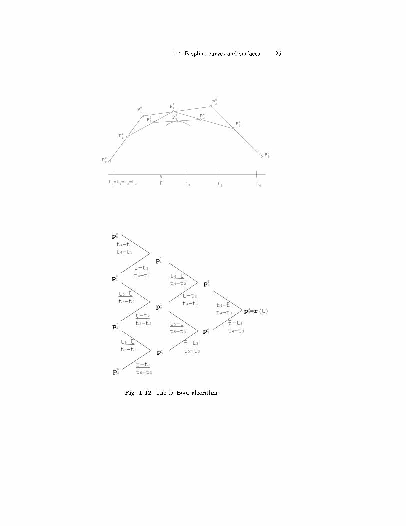
1.4 B-spline curves and surfaces 25
P1
1
P2
2 P3
3 P3
2
P3
1
P3
0
P2
0
P1
0 P2
1
P0
0
t0=t1=t2=t3 t4 t5 t6t-
p00
p10
p20
p30
p11
p21
p31
p22
p32
p3=r(t)3
t4−tt4−t1
tt4−t1
−t1
tt5−t2
−t2
tt6−t3
−t3
t5−tt5−t2
t6−tt6−t3
tt4−t2
−t2
tt5−t3
−t3
tt4−t3
−t3
t4−tt4−t2
t5−tt5−t3
t4−tt4−t3
Fig. 1.12. The de Boor algorithm

26 1. Representation of Curves and Surfaces
�ji =�t� ti
ti+k�j � ti and p0j = pj : (1.72)
For j = k � 1, the B-spline basis function reduces to Nl;1 for t 2 [tl; tl+1],and pk�1
l coincides with the curve
r(�t) = pk�1l : (1.73)
The de Boor algorithm is shown graphically in Fig. 1.12 for a cubic B-splinecurve (�t 2 [t3; t4]). If we compare Figs. 1.6 and 1.12, it is obvious that thede Boor algorithm is a generalization of the de Casteljau algorithm. Thede Boor algorithm also permits the subdivision of the B-spline curve intotwo segments of the same order. In Fig. 1.12, the two new polygons arep00 p
11 p
22 p
33 and p
33 p
23 p
13 p
03.
� Knot insertion: A knot can be inserted into a B-spline curve withoutchanging the geometry of the curve [34, 313]. The new curve is identical tothe old one, with a new basis where
nXi=0
piNi;k(t) becomesn+1Xi=0
�pi �Ni;k(t) (1.74)
over T = [t0; t1; : : : ; tl; tl+1; : : :] over T = [t0; t1; : : : ; tl; �t; tl+1; : : :] ;
when a new knot �t is inserted between knots tl and tl+1. The new de Boorpoints are given by
�pi = (1� �i)pi�1 + �ipi ; (1.75)
where
�i =
8<:1 i � l� k + 10 i � l+ 1
�t�titl+k�1�ti l � k + 2 � i � l :
(1.76)
The above algorithm is also known as Boehm's algorithm [34, 35]. A moregeneral (but also more complex) insertion algorithm permitting insertionof several (possibly multiple) knots into a B-spline knot vector, known asthe Oslo algorithm, was developed by Cohen et al. [63]. Both algorithmsdue to Boehm and Cohen et al. have found wide application in CAD/CAMsystems since the early 1980's.A B-spline curve is C1 continuous in the interior of a span. Within exactarithmetic, inserting a knot does not change the curve, so it does not changethe continuity. However, if any of the control points are moved after knotinsertion, the continuity at the knot will become Ck�p�1, where p is themultiplicity of the knot. Figure 1.13 illustrates a single insertion of a knotat parameter value �t, resulting in a knot with multiplicity one.The B-spline curve can be subdivided into B�ezier segments by knot inser-tion at each internal knot until the multiplicity of each internal knot isequal to k.

1.4 B-spline curves and surfaces 27
p01 =p0
0
p10 p2
0
p30 =p4
1
p11
p21
p31t-
Fig. 1.13. Boehm's algorithm
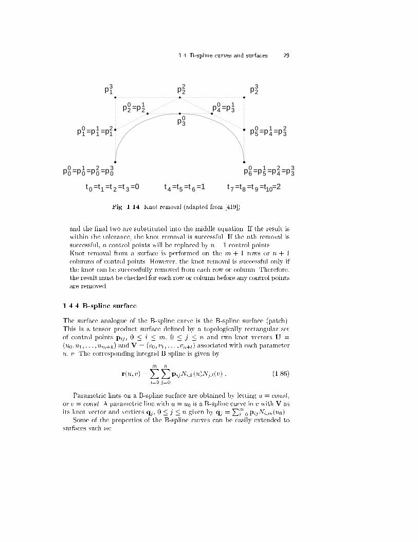
� Knot removal: Knot removal is the reverse process of knot insertion. Itis used for approximation and data reduction [242], and for data reductionin cases the curve or surface does not change neither geometrically norparametrically [419].We brie y review the latter knot removal algorithm developed by Tiller [419].To demonstrate the process, this example uses a cubic B-spline curve r(�t)given by control points (p00; : : : ;p
06) and knot vector (t0; : : : t10) where
t0 = : : : = t3 = 0, t4 = t5 = t6 = 1 and t7 = : : : = t10 = 2 as shownin Fig. 1.14. As the basis functions only guarantee C0 continuity at �t = 1,the �rst derivative may or may not be continuous there. Using the C1 con-tinuity condition (1.52), the �rst derivative will be continuous if and onlyif
(t7 � t4)(p03 � p02) = (t6 � t3)(p04 � p03) : (1.77)
Since t4 = t6 = �t,
p03 =�t� t3t7 � t3p
04 +
t7 � �t
t7 � t3p02 : (1.78)
Since p02 = p12 and p04 = p13,
p03 = �3p13 + (1� �3)p12 �3 =
�t� t3t7 � t3 : (1.79)
A similar reasoning yields the fact that a knot �t = 1 can be removed asecond time, if and only if the second derivative is continuous, yielding

28 1. Representation of Curves and Surfaces
p12 = �2p22 + (1� �2)p21 ;
p13 = �3p23 + (1� �3)p22 ; (1.80)
�i =�t� ti
ti+p+2 � ti i = 2; 3 ;
and a knot �t = 1 can be removed a third time if and only if the thirdderivative is continuous, yielding
p21 = �1p31 + (1� �1)p30 ;
p22 = �2p32 + (1� �2)p31 ;
p23 = �3p33 + (1� �3)p32 ; (1.81)
�i =�t� ti
ti+p+3 � ti i = 1; 2; 3 :
Note that there are no unknowns in (1.79), one unknown, p22, in (1.80) andtwo unknowns, p31 and p
32, in (1.81).
For the knot removal process, �rst the right hand side of (1.79) is computedand compared to p03. If they are equal within a given tolerance, the knotand p03 are removed.If the �rst knot removal is successful, equations (1.80) are solved for p22and compared:
p22 =p12 � (1� �2)p21
�2; (1.82)
p22 =p13 � �3p231� �3 : (1.83)
If the two values for p22 are the same, then the knot and control points p12and p13 are removed and control point p22 is inserted.If the second knot removal is successful, the third step is to solve the �rstand third equations of (1.81) for
p31 =p21 � (1� �1)p30
�1; (1.84)
p32 =p23 � �3p331� �3 : (1.85)
The two values are then substituted into the second equation of (1.81). Ifthe result is within tolerance of p22, then the knot is removed and controlpoints p21, p
22 and p
23 are replaced by p31 and p
32.
This can be generalized to apply to any number of removals of any par-ticular knot. For the nth removal, there will be a system of n equationswith n� 1 unknowns. If n is even, two values of the �nal unknown controlpoint will be calculated and compared. If they are within tolerance, theknot removal is successful. If n is odd, all new control points are computed
1.4 B-spline curves and surfaces 29
p00 =p0
1 =p02 =p0
3
p10 =p1
1 =p12
p13 p2
2
p30
p40 =p3
1p20 =p2
1
p23
p50 =p4
1 =p32
p60 =p5
1 =p42 =p3
3
t 0 =t1 =t 2 =t 3 =0 t 4 =t5 =t 6 =1 t 7 =t8 =t 9 =t10=2
Fig. 1.14. Knot removal (adapted from [419])
and the �nal two are substituted into the middle equation. If the result iswithin the tolerance, the knot removal is successful. If the nth removal issuccessful, n control points will be replaced by n� 1 control points.Knot removal from a surface is performed on the m + 1 rows or n + 1columns of control points. However, the knot removal is successful only ifthe knot can be successfully removed from each row or column. Therefore,the result must be checked for each row or column before any control pointsare removed.
1.4.4 B-spline surface
The surface analogue of the B-spline curve is the B-spline surface (patch).This is a tensor product surface de�ned by a topologically rectangular setof control points pij , 0 � i � m, 0 � j � n and two knot vectors U =(u0; u1; : : : ; um+k) and V = (v0; v1; : : : ; vn+l) associated with each parameteru, v. The corresponding integral B-spline is given by
r(u; v) =mXi=0
nXj=0
pijNi;k(u)Nj;l(v) : (1.86)
Parametric lines on a B-spline surface are obtained by letting u = const,or v = const. A parametric line with u = u0 is a B-spline curve in v with V asits knot vector and vertices qj , 0 � j � n given by qj =
Pmi=0 pijNi;m(u0).
Some of the properties of the B-spline curves can be easily extended tosurfaces such as:
30 1. Representation of Curves and Surfaces
� Geometry invariance property.� End points geometric property.� Convex hull property.� B-spline to B�ezier property.
However, no variation diminishing property is known for B-spline surfacepatches.
1.5 Generalization of B-spline to NURBS
Non-Uniform Rational B-Spline (NURBS) curves and surface patches [432,313] are the most popular representation method in CAD/CAM due to theirgenerality, excellent properties and incorporation in international standardssuch as IGES (Initial Graphics Exchange Speci�cation) [182] and STEP(Standard for the Exchange of Product Model Data) [428]. The NURBSfunctions have the same properties as integral B-splines, and are capable ofrepresenting a wider class of geometries. The NURBS curve is represented ina rational form
r(t) =
Pni=0 wipiNi;k(t)Pni=0 wiNi;k(t)
; (1.87)
where wi > 0 is a weighting factor and Ni;k(u) is the B-spline basis function.If all the weights are equal to one, the integral B-spline is recovered. If thenumber of control points equals the order of the NURBS curve, then thecurve reduces to a rational B�ezier curve
r(t) =
Pni=0 wibiBi;n(t)Pni=0 wiBi;n(t)
: (1.88)
The NURBS formulation permits exact representation of conics, such ascircle, ellipse and hyperbola.
Example 1.5.1. Let us express the �rst quadrant of an ellipse as a rationalB�ezier curve as shown in Fig. 1.15. A parametric representation of such ellipsesegment is given by
x = a cos �; y = b sin �; 0 � � � �
2;
where � is an angle parameter. If we set
t = tan�
2=
r1� cos �
1 + cos �;
then

1.5 Generalization of B-spline to NURBS 31
cos � =1� t2t2 + 1
; sin � =2t
t2 + 1:
Therefore the �rst quadrant of the ellipse can be described by
x(t) = a1� t2t2 + 1
; y(t) = b2t
t2 + 1; 0 � t � 1 : (1.89)
On the other hand a third order rational B�ezier curve is given by
r(t) =w0(1� t)2b0 + w12t(1� t)b1 + w2t
2b2w0(1� t)2 + w12t(1� t) + w2t2
; 0 � t � 1 : (1.90)
By equating the denominators of (1.89) and (1.90), we �nd the weights to bew0 = 1, w1 = 1 and w2 = 2. The three control points b0, b1, b2 can then beeasily obtained by the end points geometric property of the B�ezier curve asb0 = (a; 0)T , b1 = (a; b)T , and b2 = (0; b)T .
x
y
b0
b1b2
Fig. 1.15. The �rst quadrant of an ellipse described by a rational B�ezier curve
A NURBS surface patch can be represented as
r(u; v) =
Pmi=0
Pnj=0 wijpijNi;k(u)Nj;l(v)Pm
i=0
Pnj=0 wijNi;k(u)Nj;l(v)
; (1.91)
where wij > 0 is a weighting factor. This formulation allows for exact repre-sentation of quadrics, tori, surfaces of revolution and very general free-formsurfaces. If all wij = 1, the integral B-spline surface is recovered. If the num-ber of control points are equal to the order of the B-spline basis function

32 1. Representation of Curves and Surfaces
in both parameters u and v, then the NURBS surface reduces to a rationalB�ezier surface patch:
r(u; v) =
Pmi=0
Pnj=0 wijbijBi;m(u)Bj;n(v)Pm
i=0
Pnj=0 wijBi;m(u)Bj;n(v)
: (1.92)
x
y
z
b00
b01
b02
b10
b11
b12
b20
b21
b22
Fig. 1.16. 1/16 of a torus represented by a rational B�ezier surface patch
Example 1.5.2. Let us express 1/16th of a torus (in the �rst octant of a coor-dinate frame) as a rational B�ezier surface as shown in Fig. 1.16. A parametricrepresentation of such a toroidal surface patch is given by
r(�; �) = (R+ a cos�) cos �i+ (R+ a cos�) sin �j+ a sin�k; 0 � �; � � �
2;
where � and � are angle parameters, R > a, and i, j, k are unit vectors havingthe directions of the positive x, y and z axes, respectively. If we set
u = tan�
2=
r1� cos �
1 + cos �; v = tan
�
2=
s1� cos�
1 + cos�; 0 � u; v � 1 ;
then
cos � =1� u2u2 + 1
; sin � =2u
u2 + 1; cos� =
1� v2v2 + 1
; sin� =2v
v2 + 1:

1.5 Generalization of B-spline to NURBS 33
Thus the toroidal surface patch under consideration can be described by
r(u; v) =
�R+ a
1� v2v2 + 1
�1� u2u2 + 1
i+
�R+ a
1� v2v2 + 1
�2u
u2 + 1j+
2va
v2 + 1k ;
0 � u; v � 1 : (1.93)
Now we will convert this rational polynomial surface patch into a rationalB�ezier surface patch. A biquadratic B�ezier surface is given by
r(u; v) =
P2i=0
P2j=0 wijbijBi;2(u)Bj;2(v)P2
i=0
P2j=0 wijBi;2(u)Bj;2(v)
: (1.94)
By equating the denominators of (1.93) and (1.94), we �nd the weights to be
w00 = 1; w01 = 1; w02 = 2 ;
w10 = 1; w11 = 1; w12 = 2 ;
w20 = 2; w21 = 2; w22 = 4 :
The nine control points bij , 0 � i; j � 2 can then be easily obtained by theend points geometric property of the B�ezier surface as:
b00 = (R+ a; 0; 0)T , b01 = (R+ a; 0; a)T , b02 = (R; 0; a)T ;b10 = (R+ a;R+ a; 0)T ; b11 = (R+ a;R+ a; a)T ; b12 = (R;R; a)T ;b20 = (0; R+ a; 0)T ; b21 = (0; R+ a; a)T ; b22 = (0; R; a)T :


2. Di�erential Geometry of Curves
The di�erential geometry of curves and surfaces is fundamental in ComputerAided Geometric Design (CAGD). The curves and surfaces treated in di�er-ential geometry are de�ned by functions which can be di�erentiated a certainnumber of times. Books by Hilbert and Cohn-Vossen [165], Koenderink [204]provide intuitive introductions to the extensive mathematical literature onthree-dimensional shape analysis. The books by Struik [411], Willmore [443],Kreyszig [205], Lipschutz [234], do Carmo [76] o�er �rm theoretical basis tothe di�erential geometry aspects of three-dimensional shape description. Abook by Gray [136] combines the traditional textbook style and a symbolicmanipulation program Mathematica. In a recent textbook, Gallier [122]provides a thorough introduction to di�erential geometry as well as a com-prehensive treatment of a�ne and projective geometry and their applicationsto rational curves and surfaces in addition to basic topics of computationalgeometry (eg. convex hulls, Voronoi diagrams and Delaunay triangulations).We brie y review elementary di�erential geometry of curves in this chapterand surfaces in Chap. 3.
2.1 Arc length and tangent vector
Let us consider a segment of a parametric curve r = r(t) between two pointsP (r(t)) and Q (r(t+�t)) as shown in Fig. 2.1. Its length �s can be approx-imated by a chord length j�rj = jr(t+�t)� r(t)j, and by means of a Taylorexpansion we have
�s ' j�rj = jr(t+�t)� r(t)j =����drdt�t+ d2r
dt2(�t)2
���� '����drdt�����t ; (2.1)
to the �rst order approximation.Thus as point Q approaches P or in other words �t ! 0, the length �s
becomes the di�erential arc length of the curve:
ds =
����drdt���� dt = j _rjdt = p _r � _rdt : (2.2)
Here the dot _ denotes di�erentiation with respect to the parameter t. There-fore the arc length of a segment of the curve between points r(to) and r(t) can

36 2. Di�erential Geometry of Curves
P
Q
r(t+∆t)
r(t)
∆r
x
y
z
Fig. 2.1. A segment �r connecting two point P and Q on a parametric curve r(t)
be obtained as follows (provided the function t 2 [t0; t]! r(t) is one-to-onealmost everywhere):
s(t) =
Z t
to
ds =
Z t
to
p_r � _rdt =
Z t
to
p_x2(t) + _y2(t) + _z2(t)dt : (2.3)
The vector drdt is called the tangent vector at point P . This tangent vector
has a simple geometrical interpretation. The vector r(t+�t)� r(t) indicatesthe direction from r(t) to r(t +�t). If we divide the vector by �t and takethe limit as �t ! 0, then the vector will converge to the �nite magnitudevector _r(t), i.e. the tangent vector. The magnitude of the tangent vector isderived from (2.2) as
j _rj = ds
dt; (2.4)
hence the unit tangent vector becomes
t =_r
j _rj =drdtdsdt
=dr
ds� r0 : (2.5)
Here the prime 0 denotes di�erentiation with respect to the arc length. Wewill keep these notations, i.e. dot _ is for di�erentiation with respect to non-arc-length parameter t and prime 0 with respect to arc length parameter sthroughout the book. We list some useful formulae of the derivatives of arclength s with respect to parameter t and vice versa:
_s =ds
dt= j _rj =
p_r � _r ; (2.6)

2.1 Arc length and tangent vector 37
�s =d _s
dt=
_r � �rp_r � _r ; (2.7)
���s =
d�s
dt=
(_r � _r)(_r� ���r +�r � �r)� (_r � �r)2(_r � _r) 32 ; (2.8)
t0 =dt
ds=
1
j _rj =1p_r � _r ; (2.9)
t00 =dt0
ds= � _r � �r
(_r � _r)2 ; (2.10)
t000 =dt00
ds= � (�r � �r+ _r� ���r )(_r � _r)� 4(_r � �r)2
(_r � _r) 72 : (2.11)
De�nition 2.1.1. A regular (ordinary) point P on a parametric curve r =r(t) = (x(t); y(t); z(t))T is de�ned as a point where j _r(t)j 6= 0. A point whichis not a regular point is called a singular point.
De�nition 2.1.2. A parametrization r = r(t) = (x(t); y(t); z(t))T of a curvede�ned in the interval I is called an allowable representation of class r [206],if it satis�es the following:
1. the mapping r : I ! R3, t 7! r(t) = (x(t); y(t); z(t))T is one-to-one,2. the vector function r = r(t) is of class r � 1 in the interval I,3. j _r(t)j 6= 0 for all t 2 I.
A parametric curve satisfying De�nition 2.1.2 is also referred to as a regu-lar curve. The magnitude of the tangent vector ds
dt can be interpreted as a rateof change of the arc length s with respect to the parameter t and is called theparametric speed. If we assume the curve _r(t) to be regular, then by de�nitionj _r(t)j is never zero and hence ds
dt is always positive. When dsdt = 1, the curve
is said to be arc length parametrized or to have unit speed. If the parametricspeed does not vary signi�cantly, points of the curve obtained at parametervalues t0; t1; � � � ; tN corresponding to a uniform increment �t = tk � tk�1,will be nearly evenly distributed along the curve, as illustrated in Fig. 2.2.It is well known that every regular curve has an arc length parametrization[109], however, in practice it is very di�cult to �nd it analytically, due tothe fact that (2.3) is hard to integrate analytically. Pythagorean hodograph(PH) curves, introduced by Farouki and Sakkalis [108, 110], form a class ofspecial planar polynomial curves whose parametric speed is a polynomial.Accordingly, its arc length is a polynomial function s(t) of the parameter t.We provide a further review of Pythagorean hodograph curves and surfacesin Sect. 11.4.
De�nition 2.1.3. A point (x0; y0) of a planar irreducible implicit curvef(x; y) = 0 is said to be singular if f(x0; y0) = fx(x0; y0) = fy(x0; y0) = 0.

38 2. Di�erential Geometry of Curves
Parameter Space
t0 t3 t4 t5t1 t2
t0
t1
t2 t3 t4
t5
x
y
t
dsdt
Fig. 2.2. When parametric speed does not vary signi�cantly, points with uniformlyspaced parameter values are nearly uniformly spaced along a parametric curve
The unit tangent vector for implicit curves can also be derived as follows.First we start with the planar curve f(x; y) = 0. The di�erential df of theimplicit form f = 0 is zero, thus by letting fx =
@f@x and fy =
@f@y we have
df = fxdx + fydy = 0 ; (2.12)
or assuming fy 6= 0,
dy
dx= �fx
fy: (2.13)
Therefore the tangent vector on the implicit curve is given by �(fy;�fx)T ,and hence the unit tangent vector is
t = � (fy;�fx)Tq
f2x + f2y
: (2.14)
The sign depends on the sense in which s increases.As shown in Table 1.1, an implicit space curve is de�ned as the intersection
of two implicit surfaces, f(x; y; z) = 0 and g(x; y; z) = 0. As we will see inSect. 3.1, the normal vectors of these two implicit surfaces are rf and rg,respectively, where the symbol r represents the gradient vector operator
which is of the form r =�@@x ;
@@y ;
@@z
�T.
Since the tangent vector to the intersection curve is orthogonal to thenormals of the two implicit surfaces, the unit tangent vector is given by
t = � rf �rgjrf �rgj ; (2.15)
provided that the denominator is nonzero (rf 6= 0 and rg 6= 0 or in otherwords the two surfaces are nonsingular and the surfaces are not tangent toeach other at their common point under consideration). The unit tangentvector of the intersection of two implicit surfaces, when the two surfacesintersect tangentially is given in Sect. 6.4. Also here the sign depends on thesense in which s increases. A more detailed treatment of the tangent vectorof implicit curves resulting from intersection of various types of surfaces canbe found in Chap.6.

2.2 Principal normal and curvature 39
Example 2.1.1. The semi-cubical parabola, which is illustrated in Fig. 2.3,can be represented in parametric form as the curve r(t) = (t2; t3)T [226]. Theparametric speed is evaluated as j _r(t)j =pt2(4 + 9t2). It becomes zero whent = 0, hence it is singular at the origin and forms a cusp, which is illustratedin Fig. 2.3. The curve can be also represented implicitly f(x; y) = x3�y2 = 0.We can also observe that f(0; 0) = fx(0; 0) = fy(0; 0) = 0.
−0.5 0 0.5 1
−0.6
−0.4
−0.2
0
0.2
0.4
0.6
x
y
t > 0t > 0
t < 0t < 0
Fig. 2.3. A singular point occurs on a semi-cubical parabola in the form of a cusp
2.2 Principal normal and curvature
If r(s) is an arc length parametrized curve, then r0(s) is a unit vector (see(2.5)), and hence r0 � r0 = 1. Di�erentiating this relation, we obtain
r0 � r00 = 0 ; (2.16)
which states that r00 is orthogonal to the tangent vector, provided it is not anull vector. This fact can be also interpreted from the de�nition of the secondderivative r00(s)
r00(s) = lim�s!0
r0(s+�s)� r0(s)�s
: (2.17)

40 2. Di�erential Geometry of Curves
∆θ
ρ
1
1
∆s
r’ (s+∆s)r’ (s)
r’ (s+∆s)
r’ (s+∆s)−r’ (s)
r’ (s)
n
Center of curvature
∆θ
Q
P
Fig. 2.4. Derivation of the normal vector of a curve (adapted from [454])
As shown in Fig. 2.4, the direction of r0(s+�s)� r0(s) becomes perpen-dicular to the tangent vector as �s! 0. The unit vector
n =r00(s)jr00(s)j =
t0(s)jt0(s)j ; (2.18)
which has the direction and sense of t0(s) is called the unit principal normalvector at s. The plane determined by the unit tangent and normal vectorst(s) and n(s) is called the osculating plane at s. It is also well known thatthe plane through three consecutive points of the curve approaching a singlepoint de�nes the osculating plane at that point [411].
When r0(s+�s) is moved from Q to P , then r0(s), r0(s+�s) and r0(s+�s)�r0(s) form an isosceles triangle (see Fig. 2.4), since r0(s+�s) and r0(s)are unit tangent vectors. Thus we have jr0(s+�s)� r0(s)j = �� � 1 = �� =jr00(s)�sj as �s! 0 and hence
jr00(s)j = lim�s!0
��
�s= lim
�s!0
��
%��=
1
%� � : (2.19)
� is called the curvature , and its reciprocal % is called the radius of curvatureat s. It follows that
r00 = t0 = �n : (2.20)
The vector k = r00 = t0 is called the curvature vector, and measures therate of change of the tangent along the curve. By de�nition � is nonnegative,thus the sense of the normal vector is the same as that of r00(s).
The curvature for arbitrary speed (non-arc-length parametrized) curvecan be obtained as follows. First we evaluate _r and �r by the chain rule

2.2 Principal normal and curvature 41
_r =dr
ds
ds
dt= tv ; (2.21)
�r =d
dt[tv] =
dt
dsv2 + t
dv
dt= �nv2 + t
dv
dt; (2.22)
where v = dsdt is the parametric speed. Taking the cross product of _r and �r
we obtain
_r� �r = �v3t� n : (2.23)
For the planar curve, we can give the curvature � a sign by de�ning thenormal vector such that (t;n; ez) form a right-handed screw, where ez =(0; 0; 1)T as shown in Fig. 2.5. The point where the curvature changes sign iscalled an in ection point (see also Fig. 8.3).
x
y
z
tn
ezn
t
t
nκ<0
κ=0
κ>0
inflectionpoint
Fig. 2.5. Normal and tangent vectors along a 2D curve
According to this de�nition the unit normal vector of the plane curve isgiven by
n = ez � t = (� _y; _x)Tp_x2 + _y2
; (2.24)
and hence from (2.23) we have
� =(_r� �r) � ez
v3=
_x�y � _y�x
( _x2 + _y2)32
: (2.25)
For a space curve, by taking the norm of (2.23) and using (2.4), we obtain

42 2. Di�erential Geometry of Curves
� =j _r� �rjj _rj3 : (2.26)
The normal vector for the arbitrary speed curve can be obtained fromn = b � t, where b is the unit binormal vector which will be introduced inSect. 2.3 (see (2.41)).
The unit principal normal vector and curvature for implicit curves can beobtained as follows. For the planar curve the normal vector can be deducedby combining (2.14) and (2.24) yielding
n = ez � t = (fx; fy)Tq
f2x + f2y
=rfjrf j ; (2.27)
where only the + sign of t was used (although it is not necessary).We will introduce a derivative operator with respect to arc length so
that the derivation becomes simple. If we rewrite the plane implicit curveas f(x(s); y(s)) = 0 where s is arc length along the implicit curve, the totalderivative with respect to the arc length becomes
df
ds=@f
@x
dx
ds+@f
@y
dy
ds: (2.28)
Now if we replace dxds and dy
ds by using (2.5) and (2.14) (+ sign), we obtainthe derivative operator with respect to arc length
d
ds=
1
jrf j�fy
@
@x� fx @
@y
�: (2.29)
By applying the operator (2.29) to (2.14) (+ sign) and equating with �n(using (2.20) and (2.27)), we obtain
� = �fxxf2y � 2fxyfxfy + f2xfyy
(f2x + f2y )32
: (2.30)
For a 3-D implicit curve, we can deduce a derivative operator [443] similarto (2.29),
d
ds=
1
j�j��1
@
@x+ �2
@
@y+ �3
@
@z
�; (2.31)
where � is the tangent vector of the 3-D implicit curve (see (2.15)) given by
� = (�1; �2; �3) = rf �rg ; (2.32)
and

2.3 Binormal vector and torsion 43
�1 =@f
@y
@g
@z� @g
@y
@f
@z; (2.33)
�2 =@g
@x
@f
@z� @f
@x
@g
@z; (2.34)
�3 =@f
@x
@g
@y� @g
@x
@f
@y: (2.35)
By applying the derivative operator (2.31) to j�jt = � we obtain
dj�jtds
=1
j�j��1@�
@x+ �2
@�
@y+ �3
@�
@z
�; (2.36)
which gives
j�j2�n+ j�jj�j0t =��1@�
@x+ �2
@�
@y+ �3
@�
@z
�: (2.37)
Taking the cross product of j�jt = � and (2.37) yields
j�j3�b = ����1@�
@x+ �2
@�
@y+ �3
@�
@z
�: (2.38)
Thus,
� =
����� ��1 @�@x + �2@�@y + �3
@�@z
����j�j3 : (2.39)
A di�erent derivation of the curvature of a 3-D implicit curve is given in Sect.6.3.2.
2.3 Binormal vector and torsion
In Sects. 2.1 and 2.2, we have introduced the tangent and normal vectors,which are orthogonal to each other and lie in the osculating plane. Let usde�ne a unit binormal vector b such that (t;n;b) form a right-handed screw,i.e.
b = t� n; t = n� b; n = b� t ; (2.40)
which is shown in Fig. 2.6. The plane de�ned by normal and binormal vectorsis called the normal plane and the plane de�ned by binormal and tangentvectors is called the rectifying plane (see Fig. 2.6). As mentioned before, theplane de�ned by tangent and normal vectors is called the osculating plane.The binormal vector for the arbitrary speed curve with nonzero curvaturecan be obtained by using (2.23) and the �rst equation of (2.40) as follows:
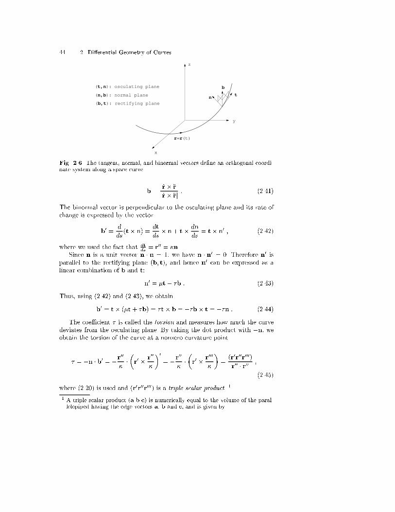
44 2. Di�erential Geometry of Curves
y
t
b
n
r=r(t)
x
z
(t,n): osculating plane
(n,b): normal plane
(b,t): rectifying plane
Fig. 2.6. The tangent, normal, and binormal vectors de�ne an orthogonal coordi-nate system along a space curve
b =_r� �r
j _r� �rj : (2.41)
The binormal vector is perpendicular to the osculating plane and its rate ofchange is expressed by the vector
b0 =d
ds(t� n) = dt
ds� n+ t� dn
ds= t� n0 ; (2.42)
where we used the fact that dtds = r00 = �n.
Since n is a unit vector n � n = 1, we have n � n0 = 0. Therefore n0 isparallel to the rectifying plane (b; t), and hence n0 can be expressed as alinear combination of b and t:
n0 = �t+ �b : (2.43)
Thus, using (2.42) and (2.43), we obtain
b0 = t� (�t+ �b) = �t � b = ��b� t = ��n : (2.44)
The coe�cient � is called the torsion and measures how much the curvedeviates from the osculating plane. By taking the dot product with �n, weobtain the torsion of the curve at a nonzero curvature point
� = �n � b0 = �r00
���r0 � r00
�
�0= �r
00
���r0 � r000
�
�=
(r0r00r000)r00 � r00 ;
(2.45)
where (2.20) is used and (r0r00r000) is a triple scalar product. 1
1 A triple scalar product (a b c) is numerically equal to the volume of the paral-lelepiped having the edge vectors a, b and c, and is given by

2.3 Binormal vector and torsion 45
The torsion for an arbitrary speed curve is given by
� =(_r�r
���r )
(_r� �r) � (_r � �r): (2.48)
The evaluation of torsion when curvature vanishes is discussed in Sect. 6.2.While the curvature is determined only in magnitude, except for plane
curves, torsion is determined both in magnitude and sign. Torsion is positivewhen the rotation of the osculating plane is in the direction of a right-handedscrew moving in the direction of t as s increases. If the torsion is zero at allpoints, the curve is planar.
The binormal vector of a 3-D implicit curve can be obtained from (2.38)as follows:
b =��
��1
@�@x + �2
@�@y + �3
@�@z
�j��
��1
@�@x + �2
@�@y + �3
@�@z
�j: (2.49)
The torsion for a 3-D implicit curve can be derived by applying the deriva-tive operator (2.31) to (2.38) [443], which gives
d
ds(j�j3�b) = (2.50)
1
j�j��1
@
@x+ �2
@
@y+ �3
@
@z
����
��1@�
@x+ �2
@�
@y+ �3
@�
@z
��;
and therefore
j�j(j�j3�)0b� j�j4��n = (2.51)��1
@
@x+ �2
@
@y+ �3
@
@z
����
��1@�
@x+ �2
@�
@y+ �3
@�
@z
��:
Taking the dot product with (2.37) we obtain
�j�j6�2� =��1@�
@x+ �2
@�
@y+ �3
@�
@z
�(2.52)
���1
@
@x+ �2
@
@y+ �3
@
@z
����
��1@�
@x+ �2
@�
@y+ �3
@�
@z
��;
from which we calculate � . An alternative approach for evaluating the torsionof 3-D implicit curves is presented in Sect. 6.3.3.
(a b c) =
�����ax bx cxay by cyaz bz cz
����� =�����ax ay azbx by bzcx cy cz
����� = (a� b) � c = a � (b� c) : (2.46)
Also a cyclic permutation maintains the value of the triple scalar product:
(a b c) = (b c a) = (c a b) : (2.47)

46 2. Di�erential Geometry of Curves
-2
-1
0
1
2
-2
-1
0
1
2
0
10
20
30
40
50
Fig. 2.7. Circular helix with a = 2, b = 3 for 0 � t � 6�
Example 2.3.1. A circular helix in parametric representation is given byr(t) = (a cos t; a sin t; bt)T . Figure 2.7 shows a circular helix with a = 2,b = 3 for 0 � t � 6�. The parametric speed is easily computed asj _r(t)j = pa2 + b2 � c, which is a constant. Therefore the curve is regularand its arc length is
s(t) =
Z t
0
j _rjdt =Z t
0
pa2 + b2dt = ct :
We can easily reparametrize the curve with arc length by replacing t by sc
yielding r = (a cos sc ; a sinsc ;
bsc )
T . The �rst three derivatives are evaluated as
r0(s) =��acsin
s
c;a
ccos
s
c;b
c
�T; r00(s) =
�� a
c2cos
s
c;� a
c2sin
s
c; 0�T
;
r000(s) =� ac3
sins
c;� a
c3cos
s
c; 0�T
:
The curvature and torsion are evaluated as follows:
�2 = r00 � r00 = a2
c4
�cos2
s
c+ sin2
s
c
�=a2
c4= constant ;
� =(r0r00r000)r00 � r00 =
(r0r00r000)�2
=c4
a2
����������
�ac sin
sc
ac cos
sc
bc
� ac2 cos
sc � a
c2 sinsc 0
ac3 sin
sc � a
c3 cossc 0
����������

2.4 Frenet-Serret formulae 47
=c4
a2b
c
a2
c5
�cos2
s
c+ sin2
s
c
�=
b
c2= constant :
Note that the circular helix has constant curvature and torsion and whenb > 0, it is a right-handed helix while when b < 0, it is a left-handed helix.
2.4 Frenet-Serret formulae
From (2.20) and (2.44), we found that
t0 = �n ; (2.53)
b0 = ��n : (2.54)
From these equations we deduce
n0 = (b� t)0 = b0 � t+ b� t0 = ��n� t+ b� (�n) = ��t+ �b :
(2.55)
In matrix form we can express the di�erential equations as0@ t0
n0
b0
1A =
0@ 0 � 0�� 0 �0 �� 0
1A0@ tnb
1A : (2.56)
Thus, t, n, b are completely determined by the curvature and torsion ofthe curve as a function of parameter s. The equations � = �(s), � = �(s)are called intrinsic equations of the curve. The formulae (2.56) are known asthe Frenet-Serret formulae and describe the motion of a moving trihedron(t; n; b) along the curve. From these t, n, b the shape of the curve can bedetermined apart for a translation and rotation. For arbitrary speed curvethe Frenet-Serret formulae are given by0
@ _t_n_b
1A =
0@ 0 v� 0�v� 0 v�0 �v� 0
1A0@ tnb
1A ; (2.57)
where v = dsdt is the parametric speed.
Example 2.4.1. As shown in Example 2.3.1 the intrinsic equations of circularhelix are given by �(s) = a
c2 , �(s) =bc2 , where c =
pa2 + b2. In this example
we derive the parametric equations of circular helix from these intrinsic equa-tions. Substituting the intrinsic equations into the Frenet-Serret equations weobtain
dt
ds=
a
c2n;
dn
ds= � a
c2t+
b
c2b;
db
ds= � b
c2n :

48 2. Di�erential Geometry of Curves
We �rst di�erentiate the �rst equation twice and the second equation oncewith respect to s, which yield
d2t
ds2=
a
c2dn
ds;
d3t
ds3=
a
c2d2n
ds2;
d2n
ds2= � a
c2dt
ds� b2
c4n ;
where the third equation is used to replace dbds . Eliminating n, dn
ds ,d2nds2 and
recognizing that t = drds , we obtain the fourth order di�erential equation
d4r
ds4+
1
c2d2r
ds2= 0 :
The general solution to this di�erential equation is given by
r(s) = C1 +C2s+C3 coss
c+C4 sin
s
c;
where C1, C2, C3 and C4 are the vector constants determined by the initialconditions. In this case we assume the following initial conditions
r(0) = (a; 0; 0)T ; r0(0) =�0;a
c;b
c
�T; r00(0) =
�� a
c2; 0; 0
�T;
r000(0) =�0;� a
c3; 0�T
;
which yield
C1 = (0; 0; 0)T ; C2 =
�0; 0;
b
c
�T;C3 = (a; 0; 0)T ; C4 = (0; a; 0)T ;
thus, we have r(s) =�a cos sc ; a sin
sc ;
bsc
�T.

3. Di�erential Geometry of Surfaces
3.1 Tangent plane and surface normal
Let us consider a curve u = u(t), v = v(t) in the parametric domain ofa parametric surface r = r(u; v) as shown in Fig. 3.1. Then r = r(t) =r(u(t); v(t)) is a parametric curve lying on the surface r = r(u; v). The tangentvector to the curve on the surface is evaluated by di�erentiating r(t) withrespect to the parameter t using the chain rule and is given by
_r(t) = ru _u+ rv _v ; (3.1)
where subscripts u and v denote partial di�erentiation with respect to u andv, respectively. The tangent plane at point P can be considered as a union
u
v zr(u,v)
r(u(t),v(t))u=u(t),v=v(t)
Parametric Space 3−D Spacex
y
Fig. 3.1. The mapping of a curve in 2-D parametric space onto a 3-D parametricsurface
of the tangent vectors of the form (3.1) for all r(t) through P as illustratedin Fig. 3.2. Point P corresponds to parameters up, vp. Since the tangentvector (3.1) consists of a linear combination of two surface tangents along iso-parametric curves ru and rv , the equation of the tangent plane at r(up; vp)in parametric form with parameters �, � is given by

50 3. Di�erential Geometry of Surfaces
Tp(�; �) = r(up; vp) + �ru(up; vp) + �rv(up; vp) : (3.2)
x
y
zr(t)=ruu+rvv
Tp
ru
rv
P
Fig. 3.2. The tangent plane at a point on a surface
The surface normal vector is perpendicular to the tangent plane (see Fig.3.3) and hence the unit normal vector is given by
N =ru � rvjru � rvj : (3.3)
By using (3.3), the equation of the tangent plane at r(up; vp) can be writtenin the implicit form as
(r � r(up; vp)) �N(up; vp) = 0 ; (3.4)
where r is a point on the tangent plane.
De�nition 3.1.1. A regular (ordinary) point P on a parametric surface isde�ned as a point where ru � rv 6= 0. A point which is not a regular point iscalled a singular point.
The condition ru � rv 6= 0 requires that at point P the vectors ru and rvdo not vanish and have di�erent directions, i.e. ru and rv are linearly inde-pendent. As we discussed in Sect. 1.3.6, in some design problems we need toemploy triangular patches de�ned by parametrization over a rectangular do-main. Such a degenerated patch can be generated by collapsing one boundarycurve into a single point or by arranging for two partial derivatives ru and rvat one of the corners of a quadrilateral patch to be collinear. In both casesru � rv has zero magnitude at the degenerate corner point and (3.3) cannotbe used. Conditions for the existence of surface normals at these degenerate

3.1 Tangent plane and surface normal 51
x
y
z
Tpru
rv
N
Fig. 3.3. The normal to the point on a surface
corner points have been discussed in [116, 92, 452, 456]. The concept of a reg-ular surface requires additional conditions beyond the existence of a tangentplane everywhere on the surface, such as absence of self-intersections. Thisconcept is presented fully in do Carmo [76].
There are essential and arti�cial singularities [443]. The essential singu-larities arise from speci�c features of the surface geometry such as the apexof a cone. The arti�cial singularities arise from the choice of parametrization.
Example 3.1.1. The elliptic cone can be described in a parametric form r =(at cos �; bt sin �; ct)T , where 0 � � � 2�, 0 � t � l and a, b, c are constants.We have
r� = (�at sin �; bt cos �; 0)T ; rt = (a cos �; b sin �; c)T ;
thus
jr� � rtj = jbct cos �ex + act sin �ey � abtezj=
qt2(b2c2 cos2 � + a2c2 sin2 � + a2b2) :
We can easily observe that the surface becomes singular only at t = 0, whichcorresponds to the apex of the cone.
The unit normal vector for an implicit surface can be derived by con-sidering two parametric curves r1 = (x1(t1); y1(t1); z1(t1))
T , r2 = (x2(t2);y2(t2); z2(t2))
T lying on an implicit surface f(x; y; z) = 0, and intersectingat point P on the surface with di�erent tangent directions. Thus we have therelations:
f(x1(t1); y1(t1); z(t1)) = 0; f(x2(t2); y2(t2); z(t2)) = 0 : (3.5)
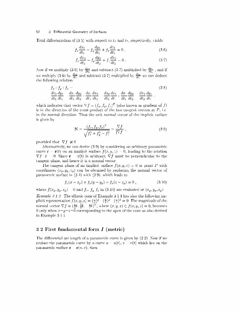
52 3. Di�erential Geometry of Surfaces
Total di�erentiation of (3.5) with respect to t1 and t2, respectively, yields
fxdx1dt1
+ fydy1dt1
+ fzdz1dt1
= 0 ; (3.6)
fxdx2dt2
+ fydy2dt2
+ fzdz2dt2
= 0 : (3.7)
Now if we multiply (3.6) by dx2dt2
and subtract (3.7) multiplied by dx1dt1
, and if
we multiply (3.6) by dy2dt2
and subtract (3.7) multiplied by dy1dt1
we can deducethe following relation
fx : fy : fz = (3.8)
dz2dt2
dy1dt1� dz1dt1
dy2dt2
:dz1dt1
dx2dt2� dz2dt2
dx1dt1
:dx1dt1
dy2dt2� dx2dt2
dy1dt1
;
which indicates that vector rf = (fx; fy; fz)T (also known as gradient of f)
is in the direction of the cross product of the two tangent vectors at P , i.e.in the normal direction. Thus the unit normal vector of the implicit surfaceis given by
N =(fx; fy; fz)
Tqf2x + f2y + f2z
=rfjrf j ; (3.9)
provided that jrf j 6= 0.Alternatively, we can derive (3.9) by considering an arbitrary parametric
curve r = r(t) on an implicit surface f(x; y; z) = 0, leading to the relationrf � _r = 0. Since r = r(t) is arbitrary, rf must be perpendicular to thetangent plane, and hence it is a normal vector.
The tangent plane of an implicit surface f(x; y; z) = 0 at point P withcoordinates (xp; yp; zp) can be obtained by replacing the normal vector ofparametric surface in (3.4) with (3.9), which leads to
fx(x � xp) + fy(y � yp) + fz(z � zp) = 0 ; (3.10)
where f(xp; yp; zp) = 0 and fx, fy fz in (3.10) are evaluated at (xp; yp; zp).
Example 3.1.2. The elliptic cone of Example 3.1.1 has also the following im-plicit representation f(x; y; z) = (xa )
2+(yb )2�( zc )2 = 0. The magnitude of the
normal vector rf = ( 2xa2 ;2yb2 ;� 2z
c2 )T , where (x; y; z) 2 f(x; y; z) = 0, becomes
0 only when x=y=z=0 corresponding to the apex of the cone as also derivedin Example 3.1.1.
3.2 First fundamental form I (metric)
The di�erential arc length of a parametric curve is given by (2.2). Now if wereplace the parametric curve by a curve u = u(t), v = v(t) which lies on theparametric surface r = r(u; v), then

3.2 First fundamental form I (metric) 53
ds =
����drdt���� dt =
����ru dudt + rvdv
dt
���� dt =p(ru _u+ rv _v) � (ru _u+ rv _v)dt
=pEdu2 + 2Fdudv +Gdv2 ; (3.11)
where
E = ru � ru; F = ru � rv ; G = rv � rv : (3.12)
The �rst fundamental form is de�ned as
I = ds2 = dr � dr = Edu2 + 2Fdudv +Gdv2 ; (3.13)
and E, F , G are called the �rst fundamental form coe�cients and play im-portant roles in many intrinsic properties of a surface. The �rst fundamentalform I can be rewritten as
I =1
E(E du+ F dv)2 +
EG� F 2
Edv2 : (3.14)
Since (ru � rv)2 = (ru � rv) � (ru � rv) = (ru � ru)(rv � rv) � (ru � rv)2 =
EG � F 2 > 01 and E = ru � ru > 0, I is positive de�nite, provided that thesurface is regular. That is I � 0 and I = 0 if and only if du = 0 and dv = 0.
Example 3.2.1. Let us compute the arc length of a curve u = t, v = t for0 � t � 1 on a hyperbolic paraboloid r(u; v) = (u; v; uv)T where 0 � u; v � 1as shown in Fig. 3.4 (a). We have
ru = (1; 0; v)T ; rv = (0; 1; u)T ;
E = ru � ru = 1 + v2; F = ru � rv = uv; G = rv � rv = 1 + u2 ;
and along the curve the �rst fundamental form coe�cients are
E = 1 + t2; F = t2; G = 1 + t2 ;
thus,
ds =pE _u2 + 2F _u _v +G _v2dt = 2
rt2 +
1
2dt :
Finally the arc length for 0 � t � 1 is given by
1 Here the vector identity
(a� b) � (c� d) = (a � c)(b � d)� (a � d)(b � c) ; (3.15)
with the special case
(a� b) � (a� b) = (a � a)(b � b)� (a � b)2 ; (3.16)
is used.

54 3. Di�erential Geometry of Surfaces
s = 2
Z 1
0
rt2 +
1
2dt =
"t
rt2 +
1
2+
1
2log
t+
rt2 +
1
2
!#10
=
r3
2+
1
2log(p2 +p3) :
(a)
x
y
z
(b)
x
y
z
Fig. 3.4. Hyperbolic paraboloid: (a) arc length along u = t, v = t, (b) areabounded by positive u and v axes and a quarter circle
The angle between two curves on a parametric surface r1 = r(u1(t); v1(t))and r2 = r(u2(t); v2(t)) can be evaluated by taking the inner product of thetangent vectors of r1 and r2, yielding
cos! =Edu1du2 + F (du1dv2 + dv1du2) +Gdv1dv2p
Edu21 + 2Fdu1dv1 +Gdv21pEdu22 + 2Fdu2dv2 +Gdv22
= Edu1ds1
du2ds2
+ F
�du1ds1
dv2ds2
+dv1ds1
du2ds2
�+G
dv1ds1
dv2ds2
: (3.17)
As a result of the above equation, the orthogonality condition for the twotangent vectors _r1 and _r2 is:
Edu1du2 + F (du1dv2 + dv1du2) +Gdv1dv2 = 0 : (3.18)
In particular when the two curves are the u and v iso-parametric curves,(3.17) reduces to
cos! =ru � rvjrujjrv j =
ru � rvpru � ruprv � rv =
FpEG
: (3.19)

3.3 Second fundamental form II (curvature) 55
Thus the iso-parametric curves are orthogonal if F = 0.The area of a small parallelogramwith vertices r(u; v), r(u+�u; v), r(u; v+
�v) and r(u+ �u; v + �v) as illustrated in Fig. 3.5, is approximated by
�A = jru�u� rv�vj =pEG� F 2�u�v ; (3.20)
or in di�erential form
dA =pEG� F 2dudv : (3.21)
r(u0+δu,v0)r(u0,v0+δv)
r(u0,v0)
δA
r(u0,v0+δv)−r(u0,v0) r(u0+δu,v0)−r(u0,v0)
Fig. 3.5. Area of small surface patch
Example 3.2.2. Let us compute the area of a region of the hyperbolic paraboloidthat is used in Example 3.2.1. The region is bounded by positive u and vaxes and a quarter circle u2 + v2 = 1 as shown in Fig. 3.4 (b). SubstitutingEG� F 2 = (1 + v2)(1 + u2)� u2v2 = 1 + u2 + v2 into (3.21), we obtain
A =
ZD
p1 + u2 + v2dudv :
To perform the integration it is easier to change variables, u = r cos �, v =r sin �, so that
A =
Z �2
0
Z 1
0
p1 + r2 r d� dr =
�
6(p8� 1) :
3.3 Second fundamental form II (curvature)
In order to quantify the curvatures of a surface S, we consider a curve Con S which passes through point P as shown in Fig. 3.6. The unit tangentvector t and the unit normal vector n of the curve C at point P are relatedby (2.20) as follows:

56 3. Di�erential Geometry of Surfaces
S P
N
kkg
kn
n
C
t
Fig. 3.6. De�nition of normal curvature
k =dt
ds= �n = kn + kg ; (3.22)
where kn is the normal curvature vector and kg is the geodesic curvaturevector which are the components of the curvature vector k of C in the surfacenormal direction and in the direction perpendicular to t in the surface tangentplane. Thus, the normal curvature vector can be expressed as
kn = �nN ; (3.23)
where �n is called the normal curvature of the surface at P in the directiont. In other words, �n is the magnitude of the projection of k onto the surfacenormal at P , with a sign determined by the orientation of the surface normalat P .
By di�erentiating N � t = 0 along the curve with respect to s we obtain
dt
ds�N+ t � dN
ds= 0 ; (3.24)
thus
�n =dt
ds�N = �t � dN
ds= �dr
ds� dNds
= �dr � dNdr � dr (3.25)
=Ldu2 + 2Mdudv +Ndv2
Edu2 + 2Fdudv +Gdv2; (3.26)
where
L = �ru �Nu; M = �12(ru �Nv + rv �Nu) = �ru �Nv = �rv �Nu ;
N = �rv �Nv : (3.27)
Since ru and rv are perpendicular to N, we have ru �N = 0 and rv �N = 0,and hence we have an alternative expression for L, M and N

3.3 Second fundamental form II (curvature) 57
L = ruu �N; M = ruv �N; N = rvv �N : (3.28)
Computation of curvatures at points where the surface representation is de-generate (see Sect. 1.3.6) is given in [452].
The numerator of (3.26) is the second fundamental form II , i.e.
II = Ldu2 + 2Mdudv +Ndv2 ; (3.29)
and L, M , N are called second fundamental form coe�cients. Therefore thenormal curvature is given by
�n =II
I=L+ 2M�+N�2
E + 2F�+G�2; (3.30)
where � = dvdu is the direction of the tangent line to C at P . We can observe
that �n at a given point P on the surface depends only on � which leads tothe following theorem due to Meusnier.
Theorem 3.3.1. All curves lying on a surface S passing through a givenpoint p 2 S with the same tangent line have the same normal curvature atthis point.
Using this theorem we can say that the normal curvature is positive whenthe center of the curvature of the normal section curve, which is a curvethrough P cut out by a plane that contains t and N; is on the same side ofthe surface normal (see Fig. 3.7 (a)). Sometimes the positive normal curvatureis de�ned in the opposite direction, i.e. the center of curvature of the normalsection curve is on the opposite side of the surface normal as illustrated inFig. 3.7 (b). In such cases (3.23) (3.30) become
kn = ��nN; �n = �III
= �L+ 2M�+N�2
E + 2F�+G�2: (3.31)
The latter convention is often used in the area of o�set curves and surfacesin the context of NC machining. Throughout this book we refer to the �rstconvention as convention (a) and to the second one as convention (b). Wehave listed all the equations, which involve changes due to this convention inthe last page of this chapter.
Suppose P is a point on a surface and Q is a point in the neighborhoodof P and r = r(u; v) is the surface containing P and Q, as in Fig. 3.8. Nowsuppose P and Q are the points r(u; v) and r(u+ du; v + dv), then Taylor'sexpansion gives
r(u+ du; v + dv) = r(u; v) + rudu+ rvdv (3.32)
+1
2(ruudu
2 + 2ruvdudv + rvvdv2) + : : : :
Therefore

58 3. Di�erential Geometry of Surfaces
center of curvature
center of curvature
N
N
P
P
(a) (b)
Fig. 3.7. De�nition of positive normal curvature: (a) �n�N = �n, (b) �n�N = ��nN
P d
Tp
Q
r=r(u,v)
Fig. 3.8. Geometrical illustration of the second fundamental form
PQ = r(u+ du; v + dv)� r(u; v) = rudu+ rvdv (3.33)
+1
2(ruudu
2 + 2ruvdudv + rvvdv2) + : : : :
Thus using (3.28), (3.29), the projection of PQ onto N is
d = PQ �N = (rudu+ rvdv) �N+1
2II ; (3.34)
where the higher order terms are neglected and since ru �N = rv �N = 0, weget
d =1
2II =
1
2(Ldu2 + 2Mdudv +Ndv2) : (3.35)
Thus jII j is equal to twice the distance from Q to the tangent plane ofthe surface at P within second order terms. We want to observe in which

3.4 Principal curvatures 59
situation d is positive and negative or in other words we want to examinein which side of the tangent plane Q lies. When d = 0, (3.35) becomesLdu2+2Mdudv+Ndv2 = 0, which can be considered as a quadratic equationin terms of du or dv. If we solve for du, assuming L 6= 0, we obtain
du =�M �pM2 � LN
Ldv ; (3.36)
which leads us to the following four cases:
� If M2 �LN < 0, there is no real root. This means there is no intersectionbetween the surface and its tangent plane except at point P . Point Pis called elliptic point (Fig. 3.9(a)). For example, an ellipsoid consistsentirely of elliptic points.
� If M2 � LN = 0 and L2 +M2 + N2 6= 0, there are double roots. Thesurface intersects its tangent plane with one line du = �M
L dv, whichpasses through point P . Point P is called parabolic point (Fig. 3.9(b)).For example, a circular cylinder consists entirely of parabolic points.
� If M2 � LN > 0, there are two roots. The surface intersects its tangent
plane with two lines du = �M�pM2�LNL dv, which intersect at point P .
Point P is called hyperbolic point (Fig. 3.9(c)). For example, a hyperboloidof revolution consists entirely of hyperbolic points.
� If L = M = N = 0, the surface and the tangent plane have a contact ofhigher order than in the preceding cases. Point P is called a at or planarpoint.
If L = 0 and N 6= 0, we can solve for dv instead of du. If L = N = 0 andM 6= 0, we have 2Mdudv = 0, thus the iso-parametric lines u = constant,v = constant will be the two intersection lines.
NN N
PP PTp
Tp
Tp
Fig. 3.9. (a) Elliptic point; (b) parabolic point; (c) hyperbolic point
3.4 Principal curvatures
As we can see from (3.30) the normal curvature at a point P depends on thedirection of � = dv
du . Now we will seek the directions in which the extrema

60 3. Di�erential Geometry of Surfaces
of principal curvature occur following Struik [411]. The extreme values of �ncan be obtained by evaluating d�n
d� = 0 of (3.30), which gives:
(E + 2F�+G�2)(N�+M)� (L+ 2M�+N�2)(G� + F ) = 0 ; (3.37)
and hence
�n =L+ 2M�+N�2
E + 2F�+G�2=M +N�
F +G�: (3.38)
Furthermore since
E + 2F�+G�2 = (E + F�) + �(F +G�) ;
L+ 2M�+N�2 = (L+M�) + �(M +N�) ;
(3.37) can be reduced to
(E + F�)(M +N�) = (L+M�)(F +G�) ; (3.39)
and hence
�n =L+ 2M�+N�2
E + 2F�+G�2=M +N�
F +G�=L+M�
E + F�: (3.40)
Therefore, the extreme values of �n satisfy the two simultaneous equations
(L� �nE)du+ (M � �nF )dv = 0 ;
(M � �nF )du+ (N � �nG)dv = 0 : (3.41)
These equations form a homogeneous linear system of equations for du, dv,which will have a nontrivial solution if and only if���� L� �nE M � �nF
M � �nF N � �nG���� = 0 ; (3.42)
where j j denotes the determinant of a matrix, or expanding
(EG� F 2)�2n � (EN +GL� 2FM)�n + (LN �M2) = 0 : (3.43)
The discriminant D of this quadratic equation in �n can be re-formulatedas
D = 4
�EG� F 2
E2
�(EM � FL)2 +
�EN �GL� 2F
E(EM � FL)
�2
;
(3.44)
after some algebraic manipulations. Thus the discriminantD is always greaterthan or equal to zero and (3.43) has real roots. The discriminant D becomes

3.4 Principal curvatures 61
zero if and only if EM � FL = 0 and EN �GL = 0 or if and only if thereis a constant k such that
L = kE; M = kF; N = kG : (3.45)
Such a point is called an umbilic and the normal curvature is the same inall directions. Therefore (3.43) has either two distinct real roots, or a doubleroot. If we set
K =LN �M2
EG� F 2; (3.46)
H =EN +GL� 2FM
2(EG� F 2); (3.47)
the quadratic equation for �n (3.43) simpli�es to:
�2n � 2H�n +K = 0 : (3.48)
The quantities K and H are called Gaussian (Gauss) curvature and meancurvature, respectively. Upon solving (3.48) for the extreme values of cur-vature, we have
�max = H +pH2 �K ; (3.49)
�min = H �pH2 �K ; (3.50)
where �max is the maximum principal curvature and �min is the minimumprincipal curvature. The directions in the tangent plane for which �n takesmaximum and minimum values are called principal directions. The corre-sponding directions in the uv-plane can be determined by using (3.40), whichleads to
� = �M � �nFN � �nG ; (3.51)
or
� = � L� �nEM � �nF ; (3.52)
where �n is replaced by either �max or �min.When the discriminant is zero or H2 = K, �n is a double root with value
equal to H and the corresponding point of the surface is an umbilical point.At an umbilical point a surface is locally a part of sphere with radius ofcurvature 1
jHj . In the special case where both K and H vanish, the point is
a at or planar point.Alternatively we can derive the principal directions by solving a quadratic
equation in �

62 3. Di�erential Geometry of Surfaces
(FN �GM)�2 + (EN �GL)�+ (EM � FL) = 0 ; (3.53)
which is deduced from (3.37). The discriminant of this equation is easilyshown to be the same as that of (3.43), and hence it is greater than or equalto zero. At an umbilical point the discriminant vanishes and (3.45) hold, thuswe have FN = GM , EN = GL and EM = FL. Therefore, the coe�cients ofthe quadratic equation become all zero and thus the principal directions arenot de�ned. When a point P on the surface is a non-umbilical point, there arealways two principal directions determined by the quadratic equations. Let�max and �min be the directions of maximum and minimum principal cur-vature in the uv-plane. Then, �max and �min satisfy the quadratic equation(3.53):
(FN �GM)�2max + (EN �GL)�max + (EM � FL) = 0 ; (3.54)
(FN �GM)�2min + (EN �GL)�min + (EM � FL) = 0 : (3.55)
From these equations we can deduce
�max + �min = � EN �GLFN �GM ; (3.56)
�max�min =EM � FLFN �GM ; (3.57)
thus,
E + F (�max + �min) +G�max�min (3.58)
=1
FN �GM [E(FN �GM)� F (EN �GL) +G(EM � FL)] = 0 :
Consequently, it is evident from (3.18) that the two tangent vectors in theprincipal directions are orthogonal.
A curve on a surface whose tangent at each point is in a principal directionat that point is called a line of curvature. Since at each (non-umbilical) pointthere are two principal directions that are orthogonal, the lines of curvaturesform an orthogonal net of lines. Figure 3.10 shows an example of the linesof curvature on a saddle-shaped surface where all points are hyperbolic. Thesolid lines correspond to the maximum principal curvature direction, whilethe dashed lines correspond to the minimum principal curvature direction(convention (a) is used). Since there is no umbilical point on the surface, wedo not encounter any singularity on the net of lines of curvature. The linesof curvature in the presence of umbilical points are discussed in Chap. 9.
This orthogonal net of lines can be used as a parametrization of a surface.In such cases, we have F = 0 (see (3.19)), and (3.41) reduce to
(L� �nE)du+Mdv = 0; Mdu+ (N � �nG)dv = 0 : (3.59)
If these equations are satis�ed by du = 0 and by dv = 0, this implies M = 0,and the two principal curvatures are �1 =
LE and �2 =
NG , in the absence of

3.4 Principal curvatures 63
x
y
z
Fig. 3.10. Lines of curvature
umbilical points. Therefore the necessary condition for the parametric linesto be lines of curvature is
F =M = 0 : (3.60)
The converse is also true and the condition is also su�cient.
Example 3.4.1. As a curve C in the xz-plane x = f(t), z = g(t) revolvesabout the z-axis, it generates a surface of revolution S. The curves C indi�erent rotated positions are called the meridians of S, while the circlesgenerated by each point on C are called the parallels of S. If we denotethe rotation angle in the xy-plane as �, the surface of revolution can beparametrized as
r = (f(t) cos �; f(t) sin �; g(t))T :
Thus,
rt = ( _f(t) cos �; _f(t) sin �; _g(t))T ; r� = (�f(t) sin �; f(t) cos �; 0)T ;and hence
E = _f2(t) + _g2(t); F = 0; G = f2(t) :
Since F = 0, (3.19) shows that the meridians and parallels are orthogonal.Furthermore we have
L =� �f _g + _f�gq_f2(t) + _g2(t)
; M = 0; N =f _gq
_f2(t) + _g2(t);
which lead us to the conclusion that the meridians and parallels of a surfaceof revolution are the lines of curvature.

64 3. Di�erential Geometry of Surfaces
3.5 Gaussian and mean curvatures
From (3.49), (3.50), it is readily seen that the Gaussian and mean curvaturesare the product and the average of the two principal curvatures, respectively:
K = �max�min ; (3.61)
H =�max + �min
2: (3.62)
The sign of the Gaussian curvature coincides with sign of LN�M2, since
K = LN�M2
EG�F 2 (see (3.46)) and EG � F 2 > 0. Consequently a point on asurface is elliptic if K > 0 (�max and �min are of the same sign), hyperbolicif K < 0 (�max and �min have di�erent signs) and parabolic if K = 0 andH 6= 0 (either �max or �min is zero), at or planar point if K = H = 0(�max = �min = 0).
3.5.1 Explicit surfaces
Very often a surface is given by an explicit form z = h(x; y). It is, therefore,convenient to have analytic equations for the Gaussian and mean curvaturesexpressed in terms of the derivatives of the height function h(x; y). As wementioned in Sect. 1.1 the explicit form can be converted into a parametricform r = (u; v; h(u; v))T where u = x and v = y. This form is often referred toasMonge form , and the surface is called a Monge patch. It is straightforwardto evaluate
E = 1 + h2x; F = hxhy; G = 1 + h2y ; (3.63)
N =(�hx;�hy; 1)Tq
1 + h2x + h2y
; (3.64)
L =hxxq
1 + h2x + h2y
; M =hxyq
1 + h2x + h2y
; N =hyyq
1 + h2x + h2y
;
(3.65)
and hence
K =LN �M2
EG� F 2=
hxxhyy � h2xy(1 + h2x + h2y)
2; (3.66)
H =EN +GL� 2FM
2(EG� F 2)=
(1 + h2x)hyy � 2hxhyhxy + (1 + h2y)hxx
2(1 + h2x + h2y)3=2
:
(3.67)

3.5 Gaussian and mean curvatures 65
Example 3.5.1. Let us compute the Gaussian and mean curvatures of thehyperbolic paraboloid z = xy (in Example 3.2.1 we used its parametric form)using the explicit formulae (3.63) to (3.67). Since
hx = y; hy = x; hxx = 0; hxy = 1; hyy = 0; N =(�y;�x; 1)Tpx2 + y2 + 1
;
we have
E = 1 + y2; F = xy; G = 1 + x2; L = 0; M =1p
x2 + y2 + 1; N = 0 ;
and hence
K = � 1
(x2 + y2 + 1)2; H = � xy
(x2 + y2 + 1)32
:
Here we can observe that the Gaussian curvature is always negative and thusall the points on a hyperbolic paraboloid are hyperbolic points. Furthermore,since L = N = 0 and M 6= 0, the surface intersects its tangent plane atthe iso-parametric lines (see Sect. 3.3 last paragraph). Also from (3.49) and(3.50) we obtain
�max =�xy +p(x2 + 1)(y2 + 1)
(x2 + y2 + 1)32
; �min =�xy �p(x2 + 1)(y2 + 1)
(x2 + y2 + 1)32
;
where it is very easy to show that �max > 0 and �min < 0 for all (x; y).
3.5.2 Implicit surfaces
Using (3.66), (3.67) for an explicit surface, we can derive equations for theGaussian and mean curvature of an implicit surface f(x; y; z) = 0. At a pointwhere fz 6= 0, z can be expressed as a function of x and y, say z = h(x; y)[166]. In such cases variables x and y are independent but z is a functionof both x and y. Since f constantly satis�es the equation f(x; y; z) = 0, thepartial di�erentiation of f with respect to the independent variable x (byholding y �xed) must vanish [166]. Thus,�
@f
@x
�y
=@f
@x+@f
@z
@z
@x= 0 ; (3.68)
where�@f@x
�yon the left-hand side is considered as f being expressed in terms
of x and y only and y is held constant in the di�erentiation with respect to x,while @f
@x on the right-hand side is considered as f being expressed in termsof x, y, z and y, z are held constant in the x di�erentiation. Similarly wehave

66 3. Di�erential Geometry of Surfaces�@f
@y
�x
=@f
@y+@f
@z
@z
@y= 0 : (3.69)
Consequently we have
hx = �fxfz; hy = �fy
fz: (3.70)
The second order partial derivatives hxx, hxy, hyy are provided by di�er-entiating (3.70). For example,
hxx = �
�@fx@x
�yfz �
�@fz@x
�yfx
f2z=
2fxfzfxz � f2xfzz � f2z fxxf3z
: (3.71)
Similarly, we have
hxy =fxfzfyz + fyfzfxz � fxfyfzz � f2z fxy
f3z; (3.72)
hyy =2fyfzfyz � f2yfzz � f2z fyy
f3z: (3.73)
Equations (3.70) to (3.73) may be substituted into (3.63) and (3.65) toobtain the �rst and second fundamental form coe�cients, and into (3.66) and(3.67) to compute the Gaussian and mean curvature of an implicit surface. Iffz = 0, alternate formulae may be found by cyclic permutation of x, y, z.
For every quadric surface, it is possible to �nd a suitable 3-D rotationsuch that the cross terms dxy, eyz and fxz cancel out in (1.15). If a quadricsurface has a center2, its axes can be translated to the center as origin so thatthe equation of the quadric surface does not have any �rst degree terms [79].Therefore after these transformations the implicit quadrics, ellipsoids, hyper-boloids of one and two sheets, elliptic cones, elliptic cylinders and hyperboliccylinders can be expressed in a standard form
f(x; y; z) = �x2
a2+ �
y2
b2+ �
z2
c2� � = 0 ; (3.74)
where �, � and � take values either -1, 0 or 1 and � takes values either 0 or1, depending on the classi�cation of quadrics (see Table 3.1).
By evaluating (3.70), (3.71), (3.72) and (3.73) for f given in (3.74), andsubstituting into (3.66) and (3.67), we obtain
2 A center of a quadric surface is de�ned as a point bisecting every chord passingthrough it [79]. Here chord is a line which joins two points on a surface. Ellip-soids and hyperboloids have centers, while paraboloids do not have centers. Theelliptic/hyperbolic cylinder is a limiting case of the ellipsoid/hyperboloid andthe elliptic cone is asymptotic to hyperboloids of one and two sheets.
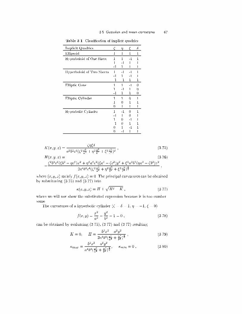
3.5 Gaussian and mean curvatures 67
Table 3.1. Classi�cation of implicit quadrics
Implicit Quadrics � � � �
Ellipsoid 1 1 1 1
Hyperboloid of One Sheet 1 1 -1 11 -1 1 1-1 1 1 1
Hyperboloid of Two Sheets 1 -1 -1 1-1 1 -1 1-1 -1 1 1
Elliptic Cone 1 1 -1 01 -1 1 0-1 1 1 0
Elliptic Cylinder 1 1 0 11 0 1 10 1 1 1
Hyperbolic Cylinder 1 -1 0 1-1 1 0 11 0 -1 1-1 0 1 10 1 -1 10 -1 1 1
K(x; y; z) =����
a2b2c2(�2 x2
a4 + �2 y2
b4 + �2 z2
c4 )2; (3.75)
H(x; y; z) = (3.76)
��2b2c2(�b2 + �c2)x2 + �2a2c2(�a2 + �c2)y2 + �2a2b2(�a2 + �b2)z2
2a4b4c4(�2 x2
a4 + �2 y2
b4 + �2 z2
c4 )32
;
where (x; y; z) satisfy f(x; y; z) = 0. The principal curvatures can be obtainedby substituting (3.75) and (3.77) into
�(x; y; z) = H �pH2 �K ; (3.77)
where we will not show the substituted expression because it is too cumber-some.
The curvatures of a hyperbolic cylinder (� = � = 1, � = �1, � = 0)
f(x; y) =x2
a2� y2
b2� 1 = 0 ; (3.78)
can be obtained by evaluating (3.75), (3.77) and (3.77) resulting
K = 0; H =b2x2 � a2y2
2a4b4(x2
a4 +y2
b4 )32
; (3.79)
�max =b2x2 � a2y2
a4b4(x2
a4 +y2
b4 )32
; �min = 0 ; (3.80)

68 3. Di�erential Geometry of Surfaces
where (x; y) 2 f(x; y) = x2
a2 � y2
b2 � 1 = 0.Similarly, the curvatures of an ellipsoid (� = � = � = � = 1)
f(x; y; z) =x2
a2+y2
b2+z2
c2� 1 = 0 ; (3.81)
are evaluated as
K =1
a2b2c2�x2
a4 +y2
b4 + z2
c4
�2 ; H =x2 + y2 + z2 � a2 � b2 � c2
2a2b2c2�x2
a4 +y2
b4 + z2
c4
� 32
;
(3.82)
� =x2 + y2 + z2 � a2 � b2 � c2
2a2b2c2�x2
a4 +y2
b4 + z2
c4
� 32
(3.83)
�
r(x2 + y2 + z2 � a2 � b2 � c2)2 � 4a2b2c2
�x2
a4 +y2
b4 + z2
c4
�2a2b2c2
�x2
a4 +y2
b4 + z2
c4
� 32
;
where (x; y; z) 2 f(x; y; z) = x2
a2 + y2
b2 + z2
c2 � 1 = 0. Here we note that inthe derivation of the mean curvature in (3.82), we used (3.81) to simplifythe expression. For the case of a sphere of radius R, (3.81) simpli�es tof(x; y; z) = 1
R2 (x2 + y2 + z2) � 1 = 0, and (3.82) and (3.83) simplify to
K = 1R2 , H = � = � 1
R , which shows that a sphere is made of entirelynon at umbilics (see Sects. 9.1 and 9.2). The negative sign comes from thesign convention of the curvature (see Fig. 3.7 and Table 3.2).
Finally, the curvatures of an elliptic cone (� = � = 1, � = �1 and � = 0)
f(x; y; z) =x2
a2+y2
b2� z2
c2= 0 ; (3.84)
excluding the apex (0,0,0) are given by
K = 0; H = � x2 + y2 + z2
2a2b2c2�x2
a4 +y2
b4 + z2
c4
� 32
; (3.85)
�max = 0; �min = � x2 + y2 + z2
a2b2c2�x2
a4 +y2
b4 + z2
c4
� 32
; (3.86)
where (x; y; z) 2 f(x; y; z) = x2
a2 +y2
b2 � z2
c2 = 0. Here we also used (3.84) tosimplify the expression of mean curvature in (3.85).
3.6 Euler's theorem and Dupin's indicatrix
The normal curvatures of a surface in an arbitrary direction (in the tangentplane) at point P can be expressed in terms of principal curvatures �1 and �2

3.6 Euler's theorem and Dupin's indicatrix 69
at point P and the angle � between the arbitrary direction and the principaldirection corresponding to �1, namely,
�n = �1 cos2 �+ �2 sin
2 � : (3.87)
This is known as Euler's theorem. For simplicity, we assume that the iso-parametric curves of a surface are lines of curvature, which leads to F =M =0 (see (3.60)). Now (3.26) takes the form
�n =Ldu2 +Ndv2
Edu2 +Gdv2: (3.88)
For v = const iso-parametric lines dv = 0 and for u = const iso-parametriclines du = 0, thus the principal curvatures �1 and �2 are given by:
�1 =L
E; �2 =
N
G: (3.89)
The angle � between the direction dvdu and the principal direction corre-
sponding to �1 (dv1 = 0, u1 arbitrary) is evaluated by (3.17) as
cos� = Edu
ds
du1ds1
: (3.90)
Since ds1 =pEdu21 and ds =
pEdu2 +Gdv2 we deduce
cos� =pEdu
ds; sin� =
pGdv
ds: (3.91)
As a consequence, we have the Euler's theorem (3.87).Next we explain Euler's theorem in a more simple way. Let us consider a
section of the surface cut by a plane parallel to the tangent plane at the pointP , and at an in�nitesimal distance h > 0 from it [440]. We also consider aplane through P containing the normal vector. If we denote the intersectionpoints of the surface and the two planes by Q and Q0, the signed radius ofcurvature of this normal section by %, and the length of QQ0 by 2R as shownin Fig. 3.11, we have the relation
(j%j � h)2 +R2 = j%j2 ; (3.92)
thus
R2 = 2hj%j ; (3.93)
to the �rst order. If � is the inclination of this normal section to the principaldirection corresponding to �1, Euler's theorem provides
�1 cos2 �+ �2 sin
2 � =1
%= � 2h
R2: (3.94)

70 3. Di�erential Geometry of Surfaces
If we set
� = R cos�; � = R sin� ; (3.95)
we obtain
�2
2h%1+
�2
2h%2= �1 ; (3.96)
where %1 and %2 are principal radius of curvatures. Consequently a section ofthe surface cut by a plane parallel to the tangent plane at the point P , andat an in�nitesimal distance is a conic section. If we scale the �-� coordinatesas follows
X =�p2h
=Rp2h
cos� =pj%j cos�; (3.97)
Y =�p2h
=Rp2h
sin� =pj%j sin� ; (3.98)
we obtain
X2
%1+Y 2
%2= �1 : (3.99)
This equation determines a conic section called Dupin's indicatrix as shownin Fig. 3.12. If P is an elliptic point, both principal curvatures have the samesign, and the indicatrix is an ellipse, while if it is a hyperbolic point, theprincipal curvatures have di�erent sign and the indicatrix consists of a pair
of hyperbolas with asymptotic lines Y = �q
j%2jj%1jX . If one of the principal
curvatures vanishes, it is a parabolic point and the indicatrix yields a pair ofparallel lines.

3.6 Euler's theorem and Dupin's indicatrix 71
Center of Curvature
Q Q’
R Rh
P
Q Q’R R
Center of Curvature
h
ρ>0
N
N
ρ<0
(a) (b)
Fig. 3.11. Cross section of the surface cut by a normal plane: (a) normal curva-ture is positive, (b) normal curvature is negative (Here we followed the curvatureconvention (a); see Fig. 3.7)
Φ
Y
| ρ 2|
| ρ 1|
| ρ |
X
Φ
Y
| ρ 2|
| ρ |
X
Y
X
Φ
| ρ |
| ρ 1|
| ρ 2|
(a) (b) (c)
Fig. 3.12. Dupin's indicatrix for (a) elliptic point, (b) parabolic point, (c) hyper-bolic point

72 3. Di�erential Geometry of Surfaces
Table 3.2. A list of equations which involves a sign change due to the sign con-vention of curvature of the planar curve or the normal curvature of the surface (seeFig. 3.7). In sign convention (a) the center of curvature is on the same side of thenormal vector, while in sign convention (b) it is on the opposite direction
Equation Convention (a) Convention (b)
(2.20) r00 = t0 = �n r00 = t0 = ��n(2.22) �r = �nv2 + t dv
dt�r = ��nv2 + t dv
dt
(2.24) n = ez � t = (� _y; _x)Tp_x2+ _y2
n = t� ez =( _y;� _x)Tp
_x2+ _y2
(2.27) n = ez � t =(fx;fy)
Tpf2x+f
2y
n = t� ez =(�fx;�fy)
Tpf2x+f
2y
= rfjrf j
= � rfjrf j
(2.55) n0 = ��t (� = 0) n0 = �t (� = 0)
(3.23) kn = �nN kn = ��nN(3.25) �n = dt
ds�N = �t � dN
ds�n = � dt
ds�N = t � dN
ds
= � drds� dNds
= � dr�dNdr�dr
= drds� dNds
= dr�dNdr�dr
(3.26) �n = Ldu2+2Mdudv+Ndv2
Edu2+2Fdudv+Gdv2�n = �Ldu2+2Mdudv+Ndv2
Edu2+2Fdudv+Gdv2
(3.30) �n = III= L+2M�+N�2
E+2F�+G�2�n = � II
I= L+2M�+N�2
E+2F�+G�2
(3.38) �n = L+2M�+N�2
E+2F�+G�2�n = �L+2M�+N�2
E+2F�+G�2
= M+N�F+G�
= �M+N�F+G�
(3.41) (L� �nE)du+ (M � �nF )dv (L+ �nE)du+ (M + �nF )dv= 0 = 0(M � �nF )du+ (N � �nG)dv (M + �nF )du+ (N + �nG)dv= 0 = 0
(3.42)
��� L� �nE M � �nFM � �nF N � �nG
��� = 0
��� L+ �nE M + �nFM + �nF N + �nG
��� = 0
(3.43) (EG� F 2)�2n (EG� F 2)�2n�(EN +GL� 2FM)�n +(EN +GL� 2FM)�n+(LN �M2) = 0 +(LN �M2) = 0
(3.47) H = EN+GL�2FM2(EG�F2)
H = 2FM�EN�GL2(EG�F2)
(3.51) � = �M��nFN��nG
� = �M+�nFN+�nG
(3.52) � = � L��nEM��nF
� = � L+�nEM+�nF
(3.67) H = H =(1+h2x)hyy�2hxhyhxy+(1+h2y)hxx
2(1+h2x+h2y)
3=2
2hxhyhxy�(1+h2x)hyy�(1+h2y)hxx
2(1+h2x+h2y)
3=2
(3.88) �n = Ldu2+Ndv2
Edu2+Gdv2�n = �Ldu2+Ndv2
Edu2+Gdv2
(3.89) �1 =LE; �2 =
NG
�1 = � LE; �2 = �N
G

4. Nonlinear Polynomial Solvers and
Robustness Issues
4.1 Introduction
We have seen in Chap. 1 that curves and surfaces in CAD/CAM systems areusually represented by piecewise polynomial equations of various types. Aswe will see in the remaining chapters of this book, the governing equationsfor general interrogation problems on such curve and surface representations(intersections, distance functions, curvature extrema, etc.) reduce to solvingsystems of nonlinear polynomial equations as follows:
f(x) = 0 ; (4.1)
where f consists of n functions f1, f2; : : : ; fn, each of which is a polynomialin the l independent variables x1, x2; : : : ; xl.
Frequently such systems also include square roots of polynomials, whicharise from normalization of the normal vector and analytical expressions ofthe principal curvatures of a surface (see (2.24), (3.3), (3.49), (3.50)).
Example 4.1.1. As an illustrative example, let us consider a simple intersec-tion problem of two planar implicit polynomial (algebraic) curves. Considertwo circles x2 + y2 = 9
16 and (x� 1)2 + y2 = 14 intersecting as shown in Fig.
4.1. In this case n = l = 2, and if we set x1 = x and x2 = y, the system ofequations becomes
f1(x1; x2) = x21 + x22 �9
16= 0 ; (4.2)
f2(x1; x2) = (x1 � 1)2 + x22 �1
4= 0 : (4.3)
The roots can be obtained by eliminating x2, and solving for x1, which gives
(x1; x2) =
21
32;�p13532
!' (0:65625;�0:36309) :
In this example the degree of the polynomials and the number of variableswere low, so we could solve the system by elementary analytical (elimination)

74 4. Nonlinear Polynomial Solvers and Robustness Issues
y
x
1
1
−1
−1
Fig. 4.1. Intersection of two circles
calculations. However, most problems that arise in CAD/CAM interroga-tion have higher degrees and number of variables. Such systems of equationshave been solved in earlier approaches by local numerical techniques such asNewton-type methods which require good initial approximation to all roots[69, 126], and hence cannot provide full assurance that all roots will be found.On the other hand global techniques �nd all the roots without initial approx-imation. We will brie y introduce Newton's method in Sect. 4.2, and the restof Chap. 4 will be spent on global techniques as well as robustness issues.
4.2 Local solution methods
Newton-type methods are based on local linearization and are conceptuallysimple. They are designed to compute roots based on initial approximations.To begin with, we consider Newton's method in one variable [69, 292] wherewe want to �nd roots for f(x) = 0. If we denote the initial guess of theroot as x0, then in the neighborhood of x0 the function f(x) can be linearlyapproximated using Taylor expansion as follows:
f(x) ' f(x0) + (x� x0) _f(x0) : (4.4)
Provided that _f(xi) 6= 0, the iteration formula immediately follows:
xi+1 = xi � f(xi)_f(xi)
; i = 0; 1; 2 : : : : (4.5)
This is illustrated in Fig. 4.2(a). A modi�ed Newton's method [151] forone variable is shown in Fig. 4.2(b), where we take a fractional step as followsin order to reduce the possibility of divergence in Fig. 4.2(b) of the full stepmethod given by (4.5)

4.2 Local solution methods 75
xi+1 = xi � �f(xi)_f(xi); (4.6)
where � = max[1; 12 ;14 ; :::] such that jf(xi+1)j < jf(xi)j.
f(x)
xx
x
i
i+1
f(x ) i
f(x )i+1
(a) ( b)
xixi+1
Fig. 4.2. Newton's method for f(x) = 0
If n = l in (4.1), we can easily extend Newton's method for a singlevariable to n variables as follows:
xi+1 = xi +�xi ; (4.7)
whereJ(xi) ��xi = �f(xi) ; (4.8)
and J(xi) =h@fj@xk
iis the Jacobian matrix of (4.1) [69].
Advantages of the Newton's method are its quadratic convergence andsimplicity of implementation. Disadvantages are that for each root a goodinitial approximation is required, otherwise the method may diverge. Alsothe method cannot by itself provide full assurance that all roots have beenfound.
Example 4.2.1. Let us solve the intersection of two circles discussed in Ex-ample 4.1.1 using Newton's method. The Jacobian matrix is evaluated asfollows:
[J ]i =
� @f1@x1
@f1@x2
@f2@x1
@f2@x2
�i
=
�2x1 2x2
2(x1 � 1) 2x2
�i
:
Thus the iteration scheme becomes�x1x2
�i+1
=
�x1x2
�i
+
��x1�x2
�i
;

76 4. Nonlinear Polynomial Solvers and Robustness Issues
where �x1 and �x2 are obtained from the solution of the following linearsystem �
2x1 2x22(x1 � 1) 2x2
�i
��x1�x2
�i
= ��f1f2
�i
:
4.3 Classi�cation of global solution methods
Global solution methods are designed to compute all roots in some area ofinterest. In recent computational algebraic geometry related research, threeclasses of methods for the computation of solutions of nonlinear polynomialsystems can be distinguished [299]: (1) algebraic and hybrid techniques, (2)homotopy (continuation) methods, (3) subdivision methods. We will brie yreview these three types of techniques.
4.3.1 Algebraic and Hybrid Techniques
Algebraic techniques for solving a nonlinear polynomial system are based onelimination theory. This theory deals with the problem of eliminating oneor more variables from a system of polynomial equations, thus reducing thegiven problem to a problem of higher degree but in fewer variables. There arebasically two fundamental approaches in elimination theory: (1) Resultants,and (2) Gr�obner bases. Both of the above operate ideally in a symbolic alge-bra environment, and the coe�cients of the polynomials involved are eitherrational or real algebraic numbers. There are several algorithms for solvingnonlinear polynomial systems using the above approaches. All the algorithmsare based on some fundamental algorithm that \�nds" all the roots, real andcomplex, of a univariate polynomial. The word \�nds" means, either the al-gorithm isolates the roots using intervals and rectangles, or encodes them asalgebraic numbers, for further manipulation. Let f(x) be a polynomial withinteger coe�cients of degree m, d be a bound for the size of the coe�cients off(x), and L(d) be the number of binary digits of d. Then, the (worst) runningtimes of real root �nding algorithms are functions of m, L(d) and are given in[64]. On the other hand, bisection methods for �nding all roots of f , real andcomplex with similar running times, can be found in [441, 356]. As it can beseen from the computing times found in [441, 64, 356], there is an enormouscoe�cient growth of all the quantities involved along the way (requiring sig-ni�cant computer memory). The latter is one of the most serious problemsthat all the algorithms using these techniques su�er from.
Resultant type algorithms: A resultant is a function of the coe�cientsof a given system of polynomials and when it is zero it provides an algebraiccriterion for determining when this polynomial system has a solution. Resul-tants can be classi�ed as classical, like the Sylvester, Bezout, Macaulay and

4.3 Classi�cation of global solution methods 77
u resultants, and non-classical like the sparse resultants. A good introductionto resultants and applications can be found in [89, 408, 412, 309, 380].
Algorithms based on resultant computation have been presented in [48,257, 186, 413, 49]. They work well on systems with a small number of so-lutions M . However, on systems with large M , these algorithms su�er frome�ciency problems. The main reason for that is that �nding roots of highdegree univariate polynomials can be a very slow procedure, as discussedabove, due to the use of exact arithmetic.
Gr�obner bases type algorithms: The theory of Gr�obner bases wasdeveloped by Buchberger [46]. Gr�obner bases are very special and usefulbases (generator sets) for a special class of subsets of polynomial rings in lvariables, called polynomial ideals. They are named after Gr�obner who wasBuchberger's thesis advisor. Gr�obner bases can be thought of as a generaliza-tion of Euclid's algorithm for computing the greatest common divisor of twopolynomials and of Gauss' triangularization algorithm for linear systems.
The usefulness of Gr�obner basis for solving nonlinear polynomial sys-tems comes from the fact that, whenever the system has a �nite num-ber of solutions, Gr�obner basis provide an equivalent system of triangularform. Algorithms using Gr�obner bases use the above fact, and appear in[47, 217, 227, 115, 444]. Using Gr�obner bases, polynomial systems are con-verted to polynomial triangular systems, which can be solved by backwardsubstitution, much in the manner of the Gauss' triangularization algorithmfor linear systems.
If the system has a �nite number of solutions in the a�ne plane, as wellas in the projective plane, then a Gr�obner basis can be computed in O(ml)time, where m is the highest degree among the polynomials and l is the num-ber of variables. In case, however, that the system is not zero-dimensional atin�nity, the time becomes O(ml2 ). These bounds do not take into account thecoe�cient growth. Gr�obner basis algorithms work well on systems with fewroots. This is one reason they have been considered seriously as a practicalequation-solving tool. But when their complexity is measured as a functionof the number of solutions, their performance is poor. As reported in [258],these algorithms frequently exhaust memory and computer resources evenfor low number of equations n and variables l (e.g. n; l � 5 ) and moder-ate degrees m. To overcome this di�culty, algorithms that combine resul-tant and linear algebra techniques are more promising concerning e�ciency[15, 287, 259, 258]. These algorithms are generally hybrid and are based onalgebraic and numerical analysis methods. In particular, this approach basedon resultants transforms the problem into a sequence of eigenvalue problems.This method has found extensive application in various types of intersectionproblems [211].

78 4. Nonlinear Polynomial Solvers and Robustness Issues
4.3.2 Homotopy (Continuation) Methods
Homotopy methods [123, 458, 218] are mathematically elegant, but unfortu-nately, investigation of such methods indicates that they tend to be numer-ically ill-conditioned. If we try to get around this problem by implementingthe algorithm in rational arithmetic, we end up with enormous memory re-quirements because we have to solve large systems of complex initial valueproblems (IVP). Interval methods can be applied to the solution of theseIVPs but they can be slow in practice [258].
4.3.3 Subdivision Methods
Subdivision methods [220, 332, 285, 391, 401, 133] are generally e�cient (in�nding simple intersections) and stable. Therefore, they are the most fre-quently used methods in practice. As we will see, they can be combined withinterval methods to numerically guarantee that certain subdomains do notcontain solutions. Interval Newton methods [272, 131, 190, 27, 159, 158] area promising class of subdivision methods. However, the subdivision methodsare not as general as algebraic methods, since they are only capable of isolat-ing zero-dimensional solutions. Furthermore, although the chances, that allroots have been found, increase as the resolution tolerance is lowered, thereis no certainty that each root has been extracted/isolated. Subdivision meth-ods typically do not provide a guarantee as to how many roots there may bein the remaining subdomains. However, if these subdomains are very small,the existence of a (single) root within these subdomains is a typical assump-tion. Lastly, subdivision techniques provide no explicit information aboutroot multiplicities without additional computation. Despite these drawbacks,subdivision methods are very useful in practice and are further describedbelow.
4.4 Projected Polyhedron algorithm
In this section we introduce an iterative global root-�nding algorithm foran n-dimensional nonlinear polynomial equation system, which belongs tothe class of subdivision methods, called Projected Polyhedron (PP) algorithmdeveloped by Sherbrooke and Patrikalakis [391]. It is easy to visualize andsimple in that it only requires two straightforward algorithms in order to im-plement it: one for subdividing multivariate polynomials in Bernstein form,and one for �nding the convex hull of a two-dimensional set of points. Thisalgorithm is an extension and generalization of earlier adaptive subdivisionalgorithms: for n = 1 used in �nding the real roots and extrema of a poly-nomial within an interval by Lane and Riesenfeld [220], and for n = 2 usedin shape interrogation by Geisow [124] or in intersecting rays with trimmedrational polynomial surface patches by Nishita et al. [285] (a method known

4.4 Projected Polyhedron algorithm 79
as B�ezier clipping). The PP algorithm has found many applications in shapeinterrogation problems (see also Grandine [133]) as we will see in subsequentsections and its convergence, rate of convergence and complexity propertiesare developed in [391].
For illustration, we will enumerate the procedures required by the PPalgorithm to �nd roots of a degree m polynomial equation f(x) = co+ c1x+c2x
2 + � � �+ cmxm = 0 over the interval a � x � b.
1. Make an a�ne parameter transformation x = a + t(b � a) such that0 � t � 1 as follows:
f(t) =
mXi=0
cMi ti; 0 � t � 1 : (4.9)
The transition from the interval a � x � b to the interval 0 � t � 1 isan a�ne map, and the polynomials are invariant under a�ne parametertransformation [92].
2. Convert the basis from monomial to Bernstein [106]:
f(t) =
mXi=0
cBi Bi;m(t) ; (4.10)
where
cBi =
iXj=0
(ij)
(mj )cMj ; (4.11)
and Bi;m(t) is the ith Bernstein polynomial of degree m.3. Create a graph of function f(t) using the linear precision property of
Bernstein polynomials (see (1.21)). Then the graph will become a B�eziercurve
f(t) =
�t
f(t)
�=
mXi=0
�imcBi
�Bi;m(t) ; (4.12)
where ( im ; cBi )
T are control points. Now the problem of �nding roots ofthe univariate polynomial has been transformed into a geometric problemof �nding the intersection of a B�ezier curve with the parameter axis, atransformation already used in Geisow [124] for surface interrogation.
4. Construct the convex hull of the B�ezier curve.5. Intersect the convex hull with the parameter axis.6. Discard the regions which do not contain roots by applying the de Castel-
jau subdivision algorithm and �nd a sub-region of [0,1] which may containthe root(s).

80 4. Nonlinear Polynomial Solvers and Robustness Issues
7. If the sub-region is su�ciently small, we conclude that there is a rootinside and return it. But when there are more than one root in the sub-region, the sub-region will not be reduced. In such case we split the regionevenly by applying the de Casteljau subdivision algorithm and we go backto 4.
Example 4.4.1. PP algorithm in one dimension.Find the roots of f(x) = �1:1x2+1:4x�0:2 = 0 where 0 � x � 2. The rootsare approximately, 0.164 and 1.108.
1. Make an a�ne parameter transformation by plugging x = 0+(2�0)t = 2tinto f(x) yielding f(t) = �4:4t2 + 2:8t� 0:2 = 0 where 0 � t � 1.
2. Convert from monomial to Bernstein basis using (4.11) as below
cBi =iX
j=0
(ij)
(2j )cMj ;
where cM0 = �0:2, cM1 = 2:8 and cM2 = �4:4, thus leading to cB0 = �0:2,cB1 = 1:2 and cB2 = �1:8.
3. Create a graph of function f(t) using linear precision property of theBernstein polynomial
t =
2Xi=0
i
2Bi;2(t) ;
yielding a B�ezier curve
f(t) =
�t
f(t)
�=
2Xi=0
�i2cBi
�Bi;2(t) :
with control points of (0, -0.2), (0.5, 1.2) and (1, -1.8).4. Construct a convex hull of the B�ezier curve, which is a triangle as shown
in Fig. 4.3.5. The convex hull intersects the t-axis with t = 0:0714 and t = 0:7.6. Discard the regions 0 � t � 0:0714 and 0:7 � t � 1, which do not contain
roots, by applying the de Casteljau algorithm. Now we have a smallerconvex hull which contains the roots (see shaded triangular in Fig. 4.3).
7. If the sub-region is su�ciently small, we conclude that there is a rootinside and return it. In this case there are two roots in the convex hull andthe sub-region does not reduce much (even after several iteration steps),thus we split the region evenly by applying the de Casteljau subdivisionalgorithm and go back to 4.
Example 4.4.2. PP algorithm in two dimensions.Let us solve the system of polynomial equations (4.2) and (4.3) over theregion �1 � x1; x2 � 1.

4.4 Projected Polyhedron algorithm 81
t
f(t)
t=0.0714 t=0.7
(0.5, 1.2)
(0, −0.2)
(1, −1.8)
Fig. 4.3. de Casteljau algorithm applied to the quadratic B�ezier curve
1. Make an a�ne parameter transformation by substituting x1 = 2u � 1and x2 = 2v � 1 into (4.2) and (4.3) so that 0 � u; v � 1, then:
f1(u; v) = 4u2 � 4u+ 4v2 � 4v +23
16= 0 ;
f2(u; v) = 4u2 � 8u+ 4v2 � 4v +19
4= 0 :
2. Convert from monomial to Bernstein basis using
cBij =iX
k=0
jXl=0
(ik)(jl )
(mk )(nl )cMkl ;
where in this case m = n = 2 leading to
c1B00 = 1:4375; c1
B01 = �0:5625; c1B02 = 1:4375 ;
c1B10 = �0:5625; c1B11 = �2:5625; c1B12 = �0:5625 ;
c1B20 = 1:4375; c1
B21 = �0:5625; c1B22 = 1:4375 ;
andc2B00 = 4:75; c2
B01 = 2:75; c2
B02 = 4:75 ;
c2B10 = 0:75; c2
B11 = �1:25; c2B12 = 0:75 ;
c2B20 = 0:75; c2
B21 = �1:25; c2B22 = 0:75 :
3. Create graphs of functions f1(u; v) and f2(u; v) using the linear precisionproperty of Bernstein polynomials. Then the graphs will become twoB�ezier surfaces as follows:

82 4. Nonlinear Polynomial Solvers and Robustness Issues
f1(u; v) =
0@ u
vf1(u; v)
1A =
2Xi=0
2Xj=0
0@ i
2j2c1Bij
1ABi;2(u)Bj;2(v) ;
f2(u; v) =
0@ u
vf2(u; v)
1A =
2Xi=0
2Xj=0
0@ i
2j2c2Bij
1ABi;2(u)Bj;2(v) :
The two B�ezier surfaces are shown in Fig. 4.4. Now the root-�ndingproblem of the bivariate polynomial system has been transformed to �ndthe intersections of three surfaces, f1(u; v), f2(u; v) and the xy-plane.Figure 4.5 shows the intersection between the plane and both B�eziersurfaces. We can easily observe that the two intersection curves are thecircles in Fig. 4.1 but trimmed in the resulting (u; v) domain.
x
y
z
x
yz
Fig. 4.4. B�ezier surfaces and their control points
4. Project the control points of f1(u; v) and f2(u; v) onto xz and yz planes.Here x = u, y = v. For each xz and yz plane, construct 2-D convex hulls.Figure 4.6 (a) shows 2-D convex hulls on the xz plane, while Fig. 4.6 (b)shows 2-D convex hulls on the yz plane. The solid line corresponds to

4.4 Projected Polyhedron algorithm 83
Fig. 4.5. B�ezier surfaces intersecting with xy-plane
convex hull of f1(u; v) and the dashed line corresponds to that of f2(u; v).
5. Intersect each 2-D convex hull on the xz plane with x (u) axis. Theparameter interval [0; 1] contains solutions of (4.2), while the interval[0:34375; 1] contains solutions of (4.3). The root is contained in thecommon interval [0:34375; 1] of u. We will repeat the same proceduresfor the 2-D convex hulls on the yz plane to �nd the common interval[0:1875; 0:8125] of v.
6. Discard the reigion [0; 0:34375] of u and regions [0; 0:1875] [0:8125; 1] of vwhich do not contain the roots by applying the de Casteljau subdivisionalgorithm to both B�ezier surfaces.
7. If the sub-regions of both parameters are su�ciently small, we concludethat there is a root. In this case, the sub-region of the v parameter willnot decrease much in size because there are two roots, while the intervaldecreases more in u parameter, since the two roots have the same uvalue. We split the sub-region of v evenly by applying the de Casteljausubdivision algorithm for both surfaces and we go back to step 4.
Many applications in shape interrogation result in systems of n nonlin-ear polynomial equations with n unknowns, referred to as balanced systems.However, there exist some problems such as tangential intersection or im-plicit curve/surface rendering consisting of n nonlinear polynomial equationswith l unknowns, where n could be larger or smaller than l. When n > l the

84 4. Nonlinear Polynomial Solvers and Robustness Issues
z
x(u)
5
−5
10
0.34375
z
y(v)
5
−5
10
*root
*root
*root
0.1875 0.8125
(a)
(b)
Fig. 4.6. Projections of control points
system is called overconstrained and when n < l it is called underconstrained.Now we will introduce an n-dimensional Projected-Polyhedron algorithmsuch that it can e�ectively handle overconstrained problems [391, 179]. Thisalgorithm can also be used in underconstrained problems but in such cases ittends to be slow (especially in the presence of in�nite roots); for such casesmore specialized algorithms are necessary (e.g. parametric surface intersec-tions where n = 3, and l = 4). In such cases the PP algorithm is used to �ndcharacteristic points e�ciently and marching methods are used to trace theintersection curves (see Sect. 5.8.2).
Suppose we are given a set of n nonlinear polynomials f1; f2; : : : ; fn, each
of which is polynomial in the independent variables x1; x2; : : : ; xl. Let m(k)i
denote the degree in xi of polynomial fk, so that the multi-index M (k) =
(m(k)1 ;m
(k)2 ; : : : ;m
(k)l ) describes all the degree information of fk. Furthermore,
suppose we are given an l-dimensional rectangular subset of Rl
B = [a1; b1]� [a2; b2]� : : :� [al; bl] : (4.13)
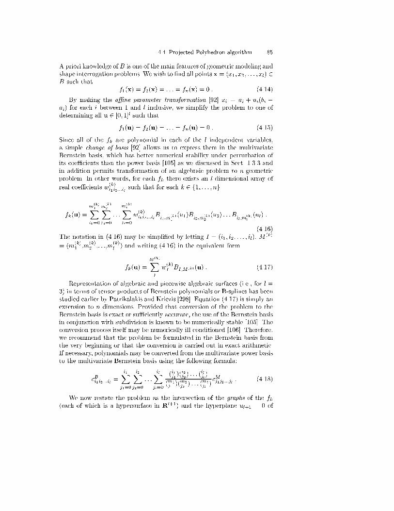
4.4 Projected Polyhedron algorithm 85
A priori knowledge of B is one of the main features of geometric modeling andshape interrogation problems. We wish to �nd all points x = (x1; x2; : : : ; xl) 2B such that
f1(x) = f2(x) = : : : = fn(x) = 0 : (4.14)
By making the a�ne parameter transformation [92] xi = ai + ui(bi �ai) for each i between 1 and l inclusive, we simplify the problem to one ofdetermining all u 2 [0; 1]l such that
f1(u) = f2(u) = : : : = fn(u) = 0 : (4.15)
Since all of the fk are polynomial in each of the l independent variables,a simple change of basis [92] allows us to express them in the multivariateBernstein basis, which has better numerical stability under perturbation ofits coe�cients than the power basis [105] as we discussed in Sect. 1.3.3 andin addition permits transformation of an algebraic problem to a geometricproblem. In other words, for each fk there exists an l-dimensional array of
real coe�cients w(k)i1i2:::il
such that for each k 2 f1; : : : ; ng
fk(u) =
m(k)1X
i1=0
m(k)2X
i2=0
: : :
m(k)
lXil=0
w(k)i1i2:::il
Bi1;m
(k)1
(u1)Bi2;m(k)2
(u2) : : : Bil;m(k)
l
(ul) :
(4.16)The notation in (4.16) may be simpli�ed by letting I = (i1; i2; : : : ; il), M
(k)
= (m(k)1 ,m
(k)2 ,: : :,m
(k)l ) and writing (4.16) in the equivalent form
fk(u) =
M(k)XI
w(k)I BI;M(k) (u) : (4.17)
Representation of algebraic and piecewise algebraic surfaces (i.e., for l =3) in terms of tensor products of Bernstein polynomials or B-splines has beenstudied earlier by Patrikalakis and Kriezis [298]. Equation (4.17) is simply anextension to n dimensions. Provided that conversion of the problem to theBernstein basis is exact or su�ciently accurate, the use of the Bernstein basisin conjunction with subdivision is known to be numerically stable [105]. Theconversion process itself may be numerically ill-conditioned [106]. Therefore,we recommend that the problem be formulated in the Bernstein basis fromthe very beginning or that the conversion is carried out in exact arithmetic.If necessary, polynomials may be converted from the multivariate power basisto the multivariate Bernstein basis using the following formula:
cBi1i2:::il =
i1Xj1=0
i2Xj2=0
: : :
ilXjl=0
(i1j1 )(i2j2) : : : (iljl)
(m1
j1)(m2
j2) : : : (ml
jl)cMj1j2:::jl : (4.18)
We now restate the problem as the intersection of the graphs of the fk(each of which is a hypersurface in Rl+1) and the hyperplane ul+1 = 0 of

86 4. Nonlinear Polynomial Solvers and Robustness Issues
Rl+1. This idea is designed to impart geometrical signi�cance to the coe�-cients of the polynomials and to the solution process.
Let us build a graph fk for each fk:
fk(u) = (u1; u2; : : : ; ul; fk(u))
= (u; fk(u)) : (4.19)
Clearly, (4.15) is satis�ed by the point u if and only if
f1(u) = f2(u) = : : : = fn(u) = (u; 0) : (4.20)
Using the linear precision property of the Bernstein basis (1.21), we obtainan equivalent expression for each of the uj in equation (4.19):
uj =
M(k)XI
ij
m(k)j
BI;M(k) (u) : (4.21)
Substituting (4.21) into (4.19) gives a more useful representation for the fk:
fk(u) =
M(k)XI
v(k)I BI;M(k) (u) ; (4.22)
where
v(k)I =
i1
m(k)1
;i2
m(k)2
; : : : ;il
m(k)l
; w(k)I
!: (4.23)
The v(k)I are called the control points of fk. Using the parametric hypersur-
faces fk instead of the real-valued fk permits use of the powerful convex-hullproperty of the multivariate Bernstein basis.
We assume we are given n nonlinear polynomial equations with l variablesin the power basis, where n � l, and a boxB = [a1; b1]�[a2; b2]�: : :�[al; bl], inwhich we need to determine the roots of the given system. In this case we �rstscale the box by performing an appropriate a�ne parameter transformationdescribed above to the functions fk, so that the box becomes [0; 1]l. Next weexpress the transformed nonlinear polynomial equations in the multivariateBernstein basis using (4.18). Now we summarize the PP algorithm.
1. Using the convex hull property, �nd a sub-box of [0; 1]l which containsall the roots. The essential idea behind the box generation scheme in thisalgorithm is to transform a complicated l+1-dimensional problem into aseries of l two-dimensional problems. Suppose Rl+1 can be coordinatizedwith the u1; u2; : : : ; ul+1 axes; we can then employ these steps:
a) Project the v(k)I of all of the fk into l di�erent coordinate planes;
speci�cally, the (u1; ul+1)-plane, the (u2; ul+1)-plane, and so on, upto the (ul; ul+1) plane.
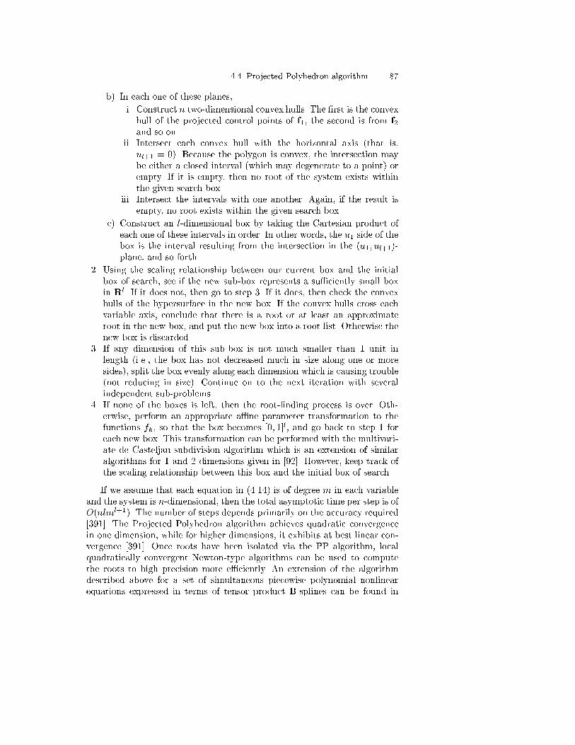
4.4 Projected Polyhedron algorithm 87
b) In each one of these planes,
i. Construct n two-dimensional convex hulls. The �rst is the convexhull of the projected control points of f1, the second is from f2and so on.
ii. Intersect each convex hull with the horizontal axis (that is,ul+1 = 0). Because the polygon is convex, the intersection maybe either a closed interval (which may degenerate to a point) orempty. If it is empty, then no root of the system exists withinthe given search box.
iii. Intersect the intervals with one another. Again, if the result isempty, no root exists within the given search box.
c) Construct an l-dimensional box by taking the Cartesian product ofeach one of these intervals in order. In other words, the u1 side of thebox is the interval resulting from the intersection in the (u1; ul+1)-plane, and so forth.
2. Using the scaling relationship between our current box and the initialbox of search, see if the new sub-box represents a su�ciently small boxin Rl. If it does not, then go to step 3. If it does, then check the convexhulls of the hypersurface in the new box. If the convex hulls cross eachvariable axis, conclude that there is a root or at least an approximateroot in the new box, and put the new box into a root list. Otherwise thenew box is discarded.
3. If any dimension of this sub-box is not much smaller than 1 unit inlength (i.e., the box has not decreased much in size along one or moresides), split the box evenly along each dimension which is causing trouble(not reducing in size). Continue on to the next iteration with severalindependent sub-problems.
4. If none of the boxes is left, then the root-�nding process is over. Oth-erwise, perform an appropriate a�ne parameter transformation to thefunctions fk, so that the box becomes [0; 1]l, and go back to step 1 foreach new box. This transformation can be performed with the multivari-ate de Casteljau subdivision algorithm which is an extension of similaralgorithms for 1 and 2 dimensions given in [92]. However, keep track ofthe scaling relationship between this box and the initial box of search.
If we assume that each equation in (4.14) is of degree m in each variableand the system is n-dimensional, then the total asymptotic time per step is ofO(nlml+1). The number of steps depends primarily on the accuracy required[391]. The Projected Polyhedron algorithm achieves quadratic convergencein one dimension, while for higher dimensions, it exhibits at best linear con-vergence [391]. Once roots have been isolated via the PP algorithm, localquadratically convergent Newton-type algorithms can be used to computethe roots to high precision more e�ciently. An extension of the algorithmdescribed above for a set of simultaneous piecewise polynomial nonlinearequations expressed in terms of tensor product B-splines can be found in

88 4. Nonlinear Polynomial Solvers and Robustness Issues
[132]. A novel feature of this extension is the normalization of the equationsin the range [-1,1] and normalization of the knot vector in each subdomainin range [0,1] at each iteration step of the process to capitalize on the higherdensity of oating point numbers in this range, thereby improving numericalrobustness of the algorithm.
Because the PP algorithm depends only on the convex hull property andability to perform subdivision and multiplication, in theory one could imple-ment the algorithm for rational B-spline entities without subdividing theminto their rational B�ezier components. Subdivision algorithms for B-splinesare well-known, and M�rken [269] has developed an algorithm for multiplyingtwo piecewise polynomials expressed in the B-spline basis. However, Zhouet al. [460] indicate that this approach sometimes tends to be more time-consuming than subdividing into rational polynomials and applying directalgebraic operations of addition and multiplication of two Bernstein forms(see Sect. 1.3.2). Piegl and Tiller [314] provide detailed description of the pro-cedures that can handle algebraic operators of NURBS curves and surfacessuch as dot and cross products, sum/di�erence and derivative operators. Theystart with decomposing the B-splines into their B�ezier components using knotinsertion, and applying the algebraic operators to the B�ezier functions and�nally recomposing the resulting B�ezier functions into B-spline form usingknot removal.
4.5 Auxiliary variable method for nonlinear systemswith square roots of polynomials
In this section we will focus on how to compute the real roots of systems ofirrational equations involving nonlinear polynomials and square roots of non-linear polynomials within a �nite box. Square roots of nonlinear polynomialsin the context of shape interrogation arise from normalization of the normalvector and analytical expressions of the principal curvatures of the surface(see (2.24), (3.3), (3.49), (3.50)). They often appear in the form of
f(x) + g(x)ph(x) = 0 ; (4.24)
where x is the unknown vector of l variables, and f(x), g(x) and h(x) aremultivariate polynomials over the box x 2 [0; 1]l.
These polynomials can be expressed in the Bernstein basis as
f(x) =
MfXI
fIBI;Mf(x) ; (4.25)
g(x) =
MgXI
gIBI;Mg(x) ; (4.26)

4.5 Auxiliary variable method for nonlinear systems with square roots of polynomials 89
h(x) =
MhXI
hIBI;Mh(x) : (4.27)
Since the square root is involved we cannot use the convex hull property ofthe Bernstein polynomial directly.
One might consider a squaring method to square out the square root, sothat the equation becomes
f2(x)� g2(x)h(x) = 0 : (4.28)
This leads to a higher degree equation, also providing extraneous roots whichare not typically necessary. The disadvantages of this squaring method arediscussed in [254]. The alternative is the auxiliary variable method which willtransform the problem into a problem of higher dimensionality. The higherdimensional formulation has been studied by Ho�mann [169] for surface in-terrogation problems. First we will introduce the auxiliary variable � suchthat
�2 = h(x) : (4.29)
Bounds a � � � b can be obtained by
a =qminIhI ; (4.30)
b =qmaxIhI : (4.31)
When minI hI is negative, we just set a=0. For convenience, we also scale� such that � � ��a
b�a , so that 0 � � � 1. Consequently, the system of ir-rational equations involving nonlinear polynomials and square roots of non-linear polynomials (4.24), which consists of one equation with l unknowns,has been transformed to a system of nonlinear polynomial equations whichconsists of two equations with l + 1 unknowns as follows:
f(x) + g(x) [a+ �(b� a)] = 0 ; (4.32)
[a+ �(b� a)]2 � h(x) = 0 ; (4.33)
where 0 � � � 1 and x 2 [0; 1]l. Note that even though we transformedthe problem into a problem of higher dimensionality, the degree of the newvariable � is only two. System (4.32) (4.33) of two polynomial equations canbe solved using the PP algorithm. A similar procedure can be used when(4.24) involves not only one but n scalar equations of the form (4.24). If theh(x) term is di�erent in each of the n equations, then system (4.32) (4.33) willbe transformed into 2n nonlinear polynomial equations in l + n unknowns.
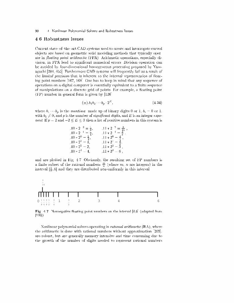
90 4. Nonlinear Polynomial Solvers and Robustness Issues
4.6 Robustness issues
Current state{of{the{art CAD systems used to create and interrogate curvedobjects are based on geometric solid modeling methods that typically oper-ate in oating point arithmetic (FPA). Arithmetic operations, especially di-vision, in FPA lead to signi�cant numerical errors. Division operation canbe avoided by four-dimensional homogeneous processing proposed by Yam-aguchi [284, 455]. Furthermore CAD systems will frequently fail as a result ofthe limited precision that is inherent to the internal representation of oat-ing point numbers [167, 168]. One has to keep in mind that any sequence ofoperations on a digital computer is essentially equivalent to a �nite sequenceof manipulations on a discrete grid of points. For example, a oating point(FP) number in general form is given by [126]
(�):b1b2 � � � bp � 2E ; (4.34)
where b1 � � � bp is the mantissa made up of binary digits 0 or 1, bi = 0 or 1,with b1 6= 0, and p is the number of signi�cant digits, and E is an integer expo-nent. If p = 2 and �2 � E � 3 then a list of positive numbers in this system is
:10 � 2�2 = 18 ; :11 � 2�2 = 3
16 ;:10 � 2�1 = 1
4 ; :11 � 2�1 = 38 ;
:10 � 20 = 14 ; :11 � 20 = 3
4 ;:10 � 21 = 1; :11 � 21 = 3
2 ;:10 � 22 = 2; :11 � 22 = 3 ;:10 � 23 = 4; :11 � 23 = 6 ;
and are plotted in Fig. 4.7. Obviously, the resulting set of FP numbers isa �nite subset of the rational numbers m
n (where m, n are integers) in theinterval [ 18 ; 6] and they are distributed non-uniformly in this interval.
0 1−8
1−4
3−8
1−2
3−4
3−2
3−16
1 2 3 4 6
Fig. 4.7. Nonnegative oating point numbers on the interval [0,6] (adapted from[126])
Nonlinear polynomial solvers operating in rational arithmetic (RA), wherethe arithmetic is done with rational numbers without approximation [203],are robust, but are generally memory intensive and time consuming due tothe growth of the number of digits needed to represent rational numbers

4.6 Robustness issues 91
that result from arithmetic operations on other rational numbers. On theother hand, nonlinear solvers operating in oating point arithmetic are faster,but generally not robust. Interval methods, which are described in Sect. 4.7,e�ectively solve these two problems, namely, nonlinear polynomial solversoperating in interval arithmetic (IA) are inexpensive compared to rationalarithmetic, and they are robust in eliminating regions not containing roots.
x
y
o
Fig. 4.8. Curves y = x4 and y = 0 contact tangentially at the origin (adaptedfrom [179])
Example 4.6.1. Suppose we have a degree four planar B�ezier curve whosecontrol points are given by
(�0:5; 0:0625); (�0:25;�0:0625); (0; 0:0625); (0:25;�0:0625); (0:5; 0:0625) ;
as shown in Fig. 4.8. This B�ezier curve is equivalent to the explicit curvey = x4 (�0:5 � x � 0:5). Apparently the curve intersects with x-axis tan-gentially at (x; y) = (0; 0). However, if the curve has been translated by +1in the y direction and translated back to the original position by moving by� 1
3 three times during a geometric processing session, the curve will gen-erally not be the same as the original curve if oating point arithmetic isused for the computation. For illustration, let us assume a decimal computerwith a four-digit mantissa, and the computer rounds o� intelligently ratherthan truncating. Then the rational number � 1
3 will be stored in the decimalcomputer as �0:3333� 100 and after the processing the new control pointswill be
(�0:5; 0:0631); (�0:25;�0:0624); (0; 0:0631); (0:25;�0:0624); (0:5; 0:0631) :
If we evaluate the curve at parameter value t = 0:5, we obtain (0, 0.00035)instead of (0,0). Therefore there exists a numerical gap which could later leadto inconsistency between topological structures and geometric equations. Forexample, if these new control points are used for computing intersections with

92 4. Nonlinear Polynomial Solvers and Robustness Issues
the x-axis, the algorithm will return no solutions when the tolerance for thefunction value is smaller than 0.00035.
The above problem illustrates the case when the error is created during theformulation of the governing equations by various algebraic transformations.
Example 4.6.2. This example �nds the roots of a cubic polynomial equation(x� 0:1)(x� 0:6)(x� 0:7) = 0 by the PP method over an interval 0 � x � 1operating in FPA. Conversion to the Bernstein form was performed in exactarithmetic. This particular example was run at a tolerance of 10�4 and thebinary subdivision was conducted when the box size did not reduce morethan 5% from the previous step. The algorithm output is listed in Table 4.1.At iteration 9, PP algorithm loses the root 0.7 due to oating point rounding.
Table 4.1. (x� 0:1)(x� 0:6)(x� 0:7) = 0 solved by PP method operating in FPA(adapted from [254])
Iter Bounding Box (FPA) Message
1 [0,1]
2 [0.0763636363636364, 0.856]
3 [0.098187732239346, 0.770083868323999]
4 [0.0999880766853688, 0.72387404781026] Binary Subdivision
5 [0.402239977003124, 0.704479954527487]
6 [0.550441290533288, 0.700214508664293]
7 [0.591018492648952, 0.700000534482207]
8 [0.599458794784619, 0.700000000003332] Binary Subdivision
9 [0.649998841568898, 0.699999999999999] No Root in Box
10 [0.599997683137796, 0.649998841568898] Root Found in Box
11 [0.099999999478761, 0.402239977003124] Root Found in Box
This example illustrates another serious problem which arises from theusage of FPA in shape interrogation. To remedy such problems interval arith-metic research in geometric modeling has become quite active as we will seein subsequent Sects. 4.7 to 4.9.
4.7 Interval arithmetic
Interval techniques, primarily interval Newton's methods combined with bi-section to ensure convergence, have been the focus of signi�cant attention,see for example Kearfott [191], Neumaier [283]. Interval methods have been

4.7 Interval arithmetic 93
applied in geometric modeling and CAD. For example, Mudur and Koparkar[276], Toth [421], Enger [90], Du� [80] and Snyder [399, 398] applied inter-val algorithms to geometry processing, whereas Sederberg and Farouki [376],Sederberg and Buehler [374] and Tuohy et al. [424] applied interval meth-ods in approximation problems. In [376] Sederberg and Farouki introducedthe concept of interval B�ezier curve. Tuohy and Patrikalakis [425] appliedinterval methods in the representation of functions with uncertainty, such asgeophysical property maps. Tuohy et al. [423] and Hager [147] applied in-terval methods in robotics. Bliek [27] studied interval Newton methods fordesign automation and inclusion monotonicity properties in interval arith-metic for solving the consistency problem associated with a hierarchical de-sign methodology. Interval methods are also applied in the context of solvingsystems of nonlinear polynomial equations [178, 179, 253, 254], which we willbrie y review in Sect. 4.8. More recently, Hu et al. [180, 181] extended theconcept of interval B�ezier curves [376] to interval non-uniform rational B-splines (INURBS) curves and surfaces. INURBS di�er from classical NURBSin that the real numbers representing control point coordinates are replacedby interval numbers. In other words, the control point vectors are replacedby rectangular boxes. This implies that in 3-D space an INURBS curve rep-resents a slender tube and an INURBS surface patch represents a thin shell,if the intervals are chosen su�ciently small. The numerical and geometricproperties of interval B-spline curves and surfaces are analyzed in Shen andPatrikalakis [386], while their use in solid modeling is presented in Hu et al.[179, 178, 180, 181], and boundary representation model recti�cation in Shen[385], Shen et al. [388], Patrikalakis et al. [302] and Sakkalis et al. [359].
An interval is a set of real numbers de�ned below [272]:
[a; b] = fxja � x � bg : (4.35)
Two intervals [a; b] and [c; d] are said to be equal if
a = c and b = d : (4.36)
The intersection of two intervals is empty or [a; b] \ [c; d] = ;, if eithera > d or c > b ; (4.37)
otherwise,
[a; b] \ [c; d] = [max(a; c);min(b; d)] : (4.38)
The union of the two intersecting intervals is
[a; b] [ [c; d] = [min(a; c);max(b; d)] : (4.39)
An order of intervals is de�ned by
[a; b] < [c; d] if and only if b < c : (4.40)

94 4. Nonlinear Polynomial Solvers and Robustness Issues
The width of an interval [a; b] is b� a.The absolute value is
j[a; b]j = max(jaj; jbj) : (4.41)
Example 4.7.1.
[2; 4] \ [3; 5] = [max(2; 3);min(4; 5)] = [3; 4]
[2; 4] [ [3; 5] = [min(2; 3);max(4; 5)] = [2; 5]
j[�7;�2]j = max(j � 7j; j � 2j) = 7
Interval arithmetic operations are de�ned by
[a; b] � [c; d] = fx � y j x 2 [a; b] and y 2 [c; d]g ; (4.42)
where � represents an arithmetic operation � 2 f+;�; �; =g. Using the endpoints of the two intervals, we can rewrite equation (4.42) as follows:
[a; b] + [c; d] = [a+ c; b+ d] ;
[a; b]� [c; d] = [a� d; b� c] ; (4.43)
[a; b] � [c; d] = [min(ac; ad; bc; bd);max(ac; ad; bc; bd)] ;
[a; b]=[c; d] = [min(a=c; a=d; b=c; b=d);max(a=c; a=d; b=c; b=d)] ;
provided 0 62 [c; d] in the division operation.
Example 4.7.2.
[2; 4] + [3; 5] = [2 + 3; 4 + 5] = [5; 9]
[2; 4]� [3; 5] = [2� 5; 4� 3] = [�3; 1][2; 4] � [3; 5] = [min(2 � 3; 2 � 5; 4 � 3; 4 � 5);max(2 � 3; 2 � 5; 4 � 3; 4 � 5)] = [6; 20]
[2; 4]=[3; 5] = [min(2=3; 2=5; 4=3; 4=5);max(2=3; 2=5; 4=3; 4=5)] = [2=5; 4=3]
Now let us introduce the algebraic properties of interval arithmetic. In-terval arithmetic is commutative,
[a; b] + [c; d] = [c; d] + [a; b]; (4.44)
[a; b] � [c; d] = [c; d] � [a; b]; (4.45)
and associative
[a; b] + ([c; d] + [e; f ]) = ([a; b] + [c; d]) + [e; f ] ; (4.46)
[a; b] � ([c; d] � [e; f ]) = ([a; b] � [c; d]) � [e; f ] : (4.47)
But it is not distributive; however, it is subdistributive
[a; b] � ([c; d] + [e; f ]) � [a; b] � [c; d] + [a; b] � [e; f ] : (4.48)
Example 4.7.3.
[1; 2] � ([1; 2]� [1; 2]) = [1; 2] � ([�1; 1]) = [�2; 2] � [1; 2] � [1; 2]� [1; 2] � [1; 2]= [1; 4]� [1; 4] = [�3; 3]

4.8 Rounded interval arithmetic and its implementation 95
4.8 Rounded interval arithmetic and its implementation
If oating point arithmetic is used to evaluate these interval arithmetic equa-tions there is no guarantee that the roundings of the bounds are performedconservatively.1 Rounded interval arithmetic (RIA) [253, 254, 4] ensures thatthe computed end points always contain the exact interval as follows:
[a; b] + [c; d] = [(a+ c)� "`; (b+ d) + "u] ;
[a; b]� [c; d] = [(a� d)� "`; (b� c) + "u] ; (4.49)
[a; b] � [c; d] = [min(a�c; a�d; b�c; b � d)� "`;max(a�c; a�d; b�c; b�d) + "u] ;
[a; b] = [c; d] = [min(a=c; a=d; b=c; b=d)� "`;max(a=c; a=d; b=c; b=d) + "u] ;
where "` and "u are the units{in{last{place denoted by ulp` and ulpu for eachseparate oating point number resulting from the oating point operationsgiving the lower and upper bounds in (4.49). When performing standardoperations for interval numbers using RIA, the lower bound is extended toinclude its previous consecutive FP number, which is smaller than the lowerbound by ulp`. Similarly, the upper bound is extended by ulpu to includeits next consecutive FP number. Thus, the width of the result is enlarged byulp` + ulpu and the resulting enlarged interval contains the exact interval.The RIA concept has been applied to topologically reliable approximation ofcurves and surfaces [58, 57], robust visualization [426], and approximation ofuncertain measured data [424].
Before describing the details of the PP algorithm in RIA, let us brie ysummarize the IEEE standard binary representation for double precision oating point numbers [4].
4.8.1 Double precision oating point arithmetic
Most commercial processors implement oating point arithmetic using therepresentation de�ned by ANSI/IEEE Std 754{1985, Standard for BinaryFloating Point Arithmetic [10]. This standard de�nes the binary represen-tation of the oating point number X in terms of a sign bit s, an integerexponent E, for Emin � E � Emax, and a p{bit signi�cand B, where
X = (�1)s2EB : (4.50)
The signi�cand B is a sequence of p bits b0b1 � � � bp�1, where bi = 0 or 1,with an implied binary point (analogous to a decimal point) between bits b0and b1. Thus, the value of B is calculated as:
1 This statement is true only for the default IEEE-754 rounding mode of roundtowards nearest [10]. The subject of hardware rounding modes will be discussedthoroughly later.

96 4. Nonlinear Polynomial Solvers and Robustness Issues
B = b0:b1b2 � � � bp�1 = b020 +
p�1Xi=1
bi2�i : (4.51)
For double precision arithmetic, the standard de�nes p = 53, Emin =�1022, and Emax = 1023. The number X is represented as a 64{bit quantitywith a 1-bit sign s, an 11{bit biased exponent e = E + 1023, and a 52{bit fractional mantissa m composed of the bit string b1b2 � � � b52. Since theexponent can always be selected such that b0 = 1 (and thus, 1 � B < 2),the value of b0 is constant and it does not need to be stored in the binaryrepresentation.
63 62 � � � 52 51 � � � 0s e m
The integer value of the 11-bit biased exponent e is calculated as:
e = e0e1 � � � e10 =10Xi=0
ei210�i : (4.52)
The standard divides the set of representable numbers into the following�ve categories:
1. If e = 2047 and m 6= 0, then the value of X is the special ag NaN (nota number).
2. If e = 2047 and m = 0, then the value of X is �1 depending upon thesign bit: positive if s = 0 and negative if s = 1.
3. If 0 < e < 2047, then X is called a normalized number, and
X = (�1)s2e�10231:m = (�1)s2e�1023
1 +
52Xi=1
bi2�i!: (4.53)
4. If e = 0 and m 6= 0, then X is called a denormalized number, and
X = (�1)s2�10220:m = (�1)s2�1022
52Xi=1
bi2�i!: (4.54)
5. If e = 0 and m = 0, then the value of X is �0 depending upon the signbit. Although they have unique binary representations, arithmetically�0 � +0.
Table 4.2 summarizes all of the representable double precision numbers.The binary representation is presented with spaces separating the four 16{bit subsets of the 64{bit value, and the symbol � separating the sign bit,exponent bits, and mantissa bits. The numbers in the �rst column refer tothe aforementioned �ve categories of representable numbers.

4.8 Rounded interval arithmetic and its implementation 97
Table 4.2. Representable double{precision numbers and special values (adaptedfrom [4])
NaN in binary representation1�11111111111�1111 1111111111111111 1111111111111111 1111111111111111
1 � � �NaN in binary representation1�11111111111�0000 0000000000000000 0000000000000000 0000000000000001
2 �1 in binary representation1�11111111111�0000 0000000000000000 0000000000000000 0000000000000000
�1:7976931348623157 � 10+308 in binary representation1�11111111110�1111 1111111111111111 1111111111111111 1111111111111111
� � ��8:9884656743115795 � 10+307 in binary representation1�11111111110�0000 0000000000000000 0000000000000000 0000000000000000
3 � � ��4:4501477170144023 � 10�308 in binary representation1�00000000001�1111 1111111111111111 1111111111111111 1111111111111111
� � ��2:2250738585072014 � 10�308 in binary representation1�00000000001�0000 0000000000000000 0000000000000000 0000000000000000
�2:2250738585072009 � 10�308 in binary representation1�00000000000�1111 1111111111111111 1111111111111111 1111111111111111
4 � � ��4:9406564584124654 � 10�324 in binary representation1�00000000000�0000 0000000000000000 0000000000000000 0000000000000001
�0:0 in binary representation1�00000000000�0000 0000000000000000 0000000000000000 0000000000000000
5 +0:0 in binary representation0�00000000000�0000 0000000000000000 0000000000000000 0000000000000000
+4:9406564584124654 � 10�324 in binary representation0�00000000000�0000 0000000000000000 0000000000000000 0000000000000001
4 � � �+2:2250738585072009 � 10�308 in binary representation0�00000000000�1111 1111111111111111 1111111111111111 1111111111111111
+2:2250738585072014 � 10�308 in binary representation0�00000000001�0000 0000000000000000 0000000000000000 0000000000000000
� � �+4:4501477170144023 � 10�308 in binary representation0�00000000001�1111 1111111111111111 1111111111111111 1111111111111111
3 � � �+8:9884656743115795 � 10+307 in binary representation0�11111111110�0000 0000000000000000 0000000000000000 0000000000000000
� � �+1:7976931348623157 � 10+308 in binary representation0�11111111110�1111 1111111111111111 1111111111111111 1111111111111111
2 +1 in binary representation0�11111111111�0000 0000000000000000 0000000000000000 0000000000000000

98 4. Nonlinear Polynomial Solvers and Robustness Issues
It is possible that the result of an operation on two normalized numberswill not itself be representable as a normalized number. Consider the nor-malized numbers x = 1:25 � 10�306 and y = 1:23 � 10�306. Clearly, x 6= y.However, in �nite precision normalized oating point arithmetic x � y = 0because x � y = 0:02� 10�306 = 2:0� 10�308, which is too small to be rep-resented as a normalized number. It is therefore rounded to the value of 0[128, pp. 23{24].
The use of denormalized numbers ensures that the relationship
x = y () x� y = 0 ; (4.55)
always holds true for all normalized numbers. It will also hold true for denor-malized numbers where jx� yj � 4:9406564584124654� 10�324, the smallestpositive representable denormalized number.
The IEEE standard can represent 2046 �252 � 9:2�1018 normalized num-bers, but only 252 � 1 � 4:5 � 1015 denormalized numbers. Denormalizednumbers are generally not encountered in routine calculations. The ratio ofdenormalized to normalized numbers is 1=2046 � 4:8 � 10�4. Furthermore,the denormalized numbers are not uniformly distributed throughout the rep-resentable oating point space; rather, they occupy two contiguous groups oneither side of 0. Certain operations, however, such as root �nding, iterativelygenerate numbers that are increasingly close to 0. Therefore it is important toallow for the possibility of encountering denormalized numbers when creatingrobust arithmetic software.
4.8.2 Extracting the exponent from the binary representation
To calculate ulp it is necessary to extract the integer value of the exponentfrom the binary representation. Recall that the value of the signi�cand B ofa double precision number X is:
B = 1 + b12�1 + b22
�2 + � � �+ b522�52 ; (4.56)
and that the double precision value X = (�1)s2EB. The value of the leastsigni�cant bit b52 is 2
�52. Thus, the value of ulp is 2E2�52 = 2E�52.The value of ulp can be computed using the standard C mathematical
functions frexp() and ldexp() [194, pp. 250-51] as follows [245, 4]:
Algorithm 4.1
#include <math.h> /* standard C math library header */
double ulp(double x){double ulp; /* ulp of x */int exp; /* exponent of x, where exp = E+1 */

4.8 Rounded interval arithmetic and its implementation 99
frexp(x, &exp); /* extract exponent of x */ulp = ldexp(0.5, exp-52); /* calculate ulp = 0.5^(exp-52) */
return ulp /* return ulp */}
(Note that the function frexp() assumes that 0:5 � B < 1. Recall that theunbiased exponent E de�ned by IEEE-754 assumes that 1 � B < 2, thusexp = E + 1. In papers [58, 57, 178, 179, 180, 181, 245, 253, 254, 424, 426]the convention of assuming 0:5 � B < 1 is followed.)
Because of the use of standard library functions, this implementation isslow. To avoid using the library functions and to construct the ulp directly,recall that the biased exponent e occupies bits 62 through 52. If we couldmanipulate the binary representation as a 64{bit integer, we could extracte by dividing by 252, which would right{shift the bit pattern by 52 bits,placing e in bits 10 through 0. The sign bit s, which would then occupy bit11, could be removed by performing a bitwise logical AND with the 64{bitmask 0 � � � 011111111111 [4].
Most commercially available processors and programming languages, how-ever, do not support 64{bit integers; generally, only 8, 16, and 32{bit integersare available. To overcome this, we can overlay the storage location of the64{bit double precision number with an array of four 16{bit (short) integers:
63 62 � � � 52 51 � � � 0s e m
short[0] short[1] short[2] short[3]63 � � � 48 47 � � � 32 31 � � � 16 15 � � � 0
In C or C++ this can be accomplished using the union data structure:
typedef union {double dp; /* the 64-bit double precision value */unsigned short sh[4]; /* overlay an array of */
} Double; /* 4 16-bit integers */
After the assignment:
double x; /* the double precision value */Double D; /* copy of x */
D.dp = x;
the exponent of the variable x can be extracted from D.sh[0], whose 16 bitscontain the sign bit s (bit 15), the 11{bit biased exponent e (bits 14 through4), and the 4 most signi�cant bits b1b2b3b4 of the mantissa m (bits 3 through0):
15 14 � � � 4 3 2 1 0s e b1b2b3b4
The biased exponent e can be extracted from D.sh[0] by performing abitwise logical AND with the 16{bit mask 0111111111110000 to zero{out the

100 4. Nonlinear Polynomial Solvers and Robustness Issues
sign bit and the four most signi�cant bits of the mantissa:
15 14 � � � 4 3 2 1 00 e 0 0 0 0
and then right{shifting e by 4 bits:15 � � � 11 10 � � � 00 � � � 0 e
Then the unbiased exponent E = e� 1023.
Some processor architectures order the four 16{bit elements of the arraysh in the reverse order, in other words, sh[0] is the rightmost (least signi�-cant) 16{bit word, not the leftmost (most signi�cant). To avoid the problem,we can de�ne the constant MSW to indicate the proper index of the left-most16 bit array element:
#define MSW 0 /* 0 if the left-most 16-bit short is sh[0] *//* 3 if the left-most 16-bit short is sh[3] */
When the ulp is a denormalized number a special case needs to be taken.Recall that ulp = 2E�52 and E must be greater than �1023. Thus, if E ��971 (or equivalently, e � 52, since e = E + 1023) then 2E�52 can only berepresented as a denormalized number with biased exponent eulp = 0 andmantissa mulp = bi, for 0 � i � 51, where:
bi =
�1 if i = e� 10 otherwise :
(4.57)
If e > 52 then ulp can be represented by the normalized number with eulp =e� 52 and mulp = 0 � � � 0.
The following function directly constructs ulp as the appropriate normal-ized or denormalized number [4]:
Algorithm 4.2static unsigned short mask[16] = { /* bit masks for bits 0 - 15 */
0x0001, 0x0002, 0x0004, 0x0008, 0x0010, 0x0020, 0x0040, 0x0080,0x0100, 0x0200, 0x0400, 0x0800, 0x1000, 0x2000, 0x4000, 0x8000};
double ulp(double x){Double U, /* ulp of x */
X; /* working copy of x */int bit, /* position of bit e-1 in 16-bit word */
e1, /* biased exponent - 1 */word; /* index of 16-bit word containing bit e-1 */
X.dp = x;X.sh[MSW] &= 0x7ff0; /* isolate exponent in 16-bit word */
/* X.sh[0] now holds the exponent in bits 14-4 */
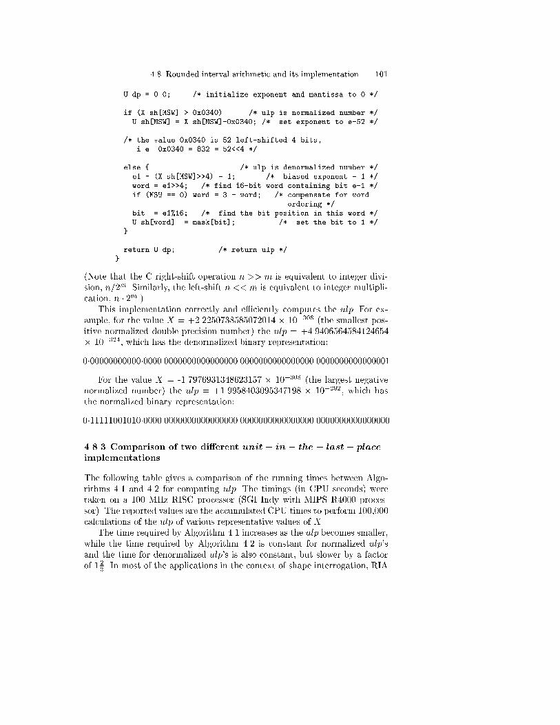
4.8 Rounded interval arithmetic and its implementation 101
U.dp = 0.0; /* initialize exponent and mantissa to 0 */
if (X.sh[MSW] > 0x0340) /* ulp is normalized number */U.sh[MSW] = X.sh[MSW]-0x0340; /* set exponent to e-52 */
/* the value 0x0340 is 52 left-shifted 4 bits,i.e. 0x0340 = 832 = 52<<4 */
else { /* ulp is denormalized number */e1 = (X.sh[MSW]>>4) - 1; /* biased exponent - 1 */word = e1>>4; /* find 16-bit word containing bit e-1 */if (MSW == 0) word = 3 - word; /* compensate for word
ordering */bit = e1%16; /* find the bit position in this word */U.sh[word] |= mask[bit]; /* set the bit to 1 */
}
return U.dp; /* return ulp */}
(Note that the C right-shift operation n >> m is equivalent to integer divi-sion, n=2m. Similarly, the left-shift n << m is equivalent to integer multipli-cation, n � 2m.)
This implementation correctly and e�ciently computes the ulp. For ex-ample, for the value X = +2.2250738585072014 � 10�308 (the smallest pos-itive normalized double precision number) the ulp = +4.9406564584124654� 10�324, which has the denormalized binary representation:
0�00000000000�0000 0000000000000000 0000000000000000 0000000000000001For the value X = -1.7976931348623157 � 10+308 (the largest negative
normalized number) the ulp = +1.9958403095347198 � 10+292, which hasthe normalized binary representation:
0�11111001010�0000 0000000000000000 0000000000000000 0000000000000000
4.8.3 Comparison of two di�erent unit� in� the � last� place
implementations
The following table gives a comparison of the running times between Algo-rithms 4.1 and 4.2 for computing ulp. The timings (in CPU seconds) weretaken on a 100 MHz RISC processor (SGI Indy with MIPS R4000 proces-sor). The reported values are the accumulated CPU times to perform 100,000calculations of the ulp of various representative values of X .
The time required by Algorithm 4.1 increases as the ulp becomes smaller,while the time required by Algorithm 4.2 is constant for normalized ulp'sand the time for denormalized ulp's is also constant, but slower by a factorof 1 23 . In most of the applications in the context of shape interrogation, RIA

102 4. Nonlinear Polynomial Solvers and Robustness Issues
Table 4.3. CPU time (in seconds) for the two implementations (adapted from [4])
X ulp (approx.) Algorithm 4.1 Algorithm 4.2
�1:25 +2:22� 10�16 0.10 0.03
�1:25� 10�100 +2:54� 10�116 1.59 0.03
�1:25� 10�200 +1:45� 10�216 3.11 0.03
�1:25� 10�285 +1:87� 10�301 4.40 0.03
�1:25� 10�295 +2:17� 10�311 y 6.68 0.05y This ulp is a denormalized number.
implementations are an order of magnitude more expensive than non{robust oating point algorithms [4].
4.8.4 Hardware rounding for rounded interval arithmetic
Since oating point numbers are represented in �nite precision, many valuesmay need to be rounded to a representable bit pattern [4]. The IEEE-754standard de�nes four rounding modes [10]: 1) Round to nearest (the de-fault mode); 2) Round to positive in�nity; 3) Round to negative in�nity; and4) Round to zero. We can examine the e�ects of these rounding modes bycalculating intermediate values between two adjacent exactly representable oating point numbers:
X1 = +2:0000000000000009
= 0�10000000000�0000 0000000000000000 0000000000000000 0000000000000010
X2 = +2:0000000000000013
= 0�10000000000�0000 0000000000000000 0000000000000000 0000000000000011
which di�er only in the last bit of the mantissa.Since IEEE-754 represents the mantissa with 52 bits, to exactly represent
the three uniformly spaced intermediary values,X1+14 (X2�X1),X1+
12 (X2�
X1), and X1+34 (X2�X1), would require two additional bits in the mantissa,
as shown in Table 4.4. To represent the negative values �X1 and �X2 onlythe sign bit is changed from 0 to 1; the exponent and mantissa bit patternsremain the same. The rounding mode round to zero is not depicted in thetable since it is not relevant to our application. Round to zero is equivalent toround to negative in�nity for positive values, and to round to positive in�nityfor negative values.
For a given unlimited precision oating- point value x, which may not beexactly representable under IEEE-754 (i.e. it may require more than 52 bitsto represent the mantissa of x), we want to construct the tightest possibleinterval [x`; xu] such that the lower bound x` is the largest possible repre-sentable number not greater than x, and the upper bound xu is the smallestpossible representable number not less than x:

4.8 Rounded interval arithmetic and its implementation 103
Table 4.4. Comparison of rounding modes (adapted from [4])
Actual Round To Nearest Round To +1Value Mantissa Rounded Represented Rounded Represented
52 bits +2 Mantissa Value Mantissa Value+2:0 : : : 009 00 : : : 010 00 00 : : : 010 +2:0 : : : 009 00 : : : 010 +2:0 : : : 009+2:0 : : : 010 00 : : : 010 01 00 : : : 010 +2:0 : : : 009 00 : : : 011 +2:0 : : : 013+2:0 : : : 011 00 : : : 010 10 00 : : : 010 +2:0 : : : 009 00 : : : 011 +2:0 : : : 013+2:0 : : : 012 00 : : : 010 11 00 : : : 011 +2:0 : : : 013 00 : : : 011 +2:0 : : : 013+2:0 : : : 013 00 : : : 011 00 00 : : : 011 +2:0 : : : 013 00 : : : 011 +2:0 : : : 013�2:0 : : : 009 00 : : : 010 00 00 : : : 010 �2:0 : : : 009 00 : : : 010 �2:0 : : : 009�2:0 : : : 010 00 : : : 010 01 00 : : : 010 �2:0 : : : 009 00 : : : 010 �2:0 : : : 009�2:0 : : : 011 00 : : : 010 10 00 : : : 010 �2:0 : : : 009 00 : : : 010 �2:0 : : : 009�2:0 : : : 012 00 : : : 010 11 00 : : : 011 �2:0 : : : 013 00 : : : 010 �2:0 : : : 009�2:0 : : : 013 00 : : : 011 00 00 : : : 011 �2:0 : : : 013 00 : : : 011 �2:0 : : : 013
Actual Round To �1Value Mantissa Rounded Represented
52 bits +2 Mantissa Value+2:0 : : : 009 00 : : : 010 00 00 : : : 010 +2:0 : : : 009+2:0 : : : 010 00 : : : 010 01 00 : : : 010 +2:0 : : : 009+2:0 : : : 011 00 : : : 010 10 00 : : : 010 +2:0 : : : 009+2:0 : : : 012 00 : : : 010 11 00 : : : 010 +2:0 : : : 009+2:0 : : : 013 00 : : : 011 00 00 : : : 011 +2:0 : : : 013�2:0 : : : 009 00 : : : 010 00 00 : : : 010 �2:0 : : : 009�2:0 : : : 010 00 : : : 010 01 00 : : : 011 �2:0 : : : 013�2:0 : : : 011 00 : : : 010 10 00 : : : 011 �2:0 : : : 013�2:0 : : : 012 00 : : : 010 11 00 : : : 011 �2:0 : : : 013�2:0 : : : 013 00 : : : 011 00 00 : : : 011 �2:0 : : : 013
x` � x � xu : (4.58)
This condition is satis�ed by rounding to negative in�nity when calculatingthe lower bound, and rounding to positive in�nity when calculating the upperbound. Note that if x is exactly representable, then x` = x = xu.
4.8.5 Implementation of rounded interval arithmetic
For implementational simplicity when switching between ulp rounding andhardware rounding, we have developed a C++ class (shown in fragmentaryform below) for interval numbers operating in oating point numbers [4]:
class Interval {
private:
double low; // lower bound of interval
double upp; // upper bound of interval
public:
Interval() { low = upp = 0.0; } // class constructors
friend Interval add(Interval, Interval, Interval &);
// utility function

104 4. Nonlinear Polynomial Solvers and Robustness Issues
};
Interval operator + (Interval a, Interval b)
// overloaded addition operator
{
Interval c;
add(a, b, c); // call appropriate utility function
return c; // return sum of a and b
}
Software rounding using the ulp is implemented by overloading the arithmeticoperators as shown in the following example for addition:
Interval add(Interval a, Interval b, Interval &c){
double low = a.low + b.low; // calculate the lower bounddouble upp = a.upp + b.upp; // calculate the upper bound
c.low = low - ulp(low); // extend the lower bound by ulpc.upp = upp + ulp(upp); // extend the upper bound by ulp
}
where ulp() is the function described previously for calculating the ulp.Hardware rounding is implemented by overloading the arithmetic opera-
tors as follows:
Interval add(Interval a, Interval b, Interval &c){
swapRM(ROUND_TO_MINUS_INFINITY); // set round to -infinity modec.low = a.low + b.low; // calculate the lower boundswapRM(ROUND_TO_PLUS_INFINITY); // set round to +infinity modec.upp = a.upp + b.upp; // calculate the upper bound
}
where swapRM() is the SGI-speci�c function for setting the IEEE-754 round-ing mode. (Although requiring the implementation of the four roundingmodes, the standard does not specify the mechanism by which the modesare set.)
The software rounding method is computationally more expensive thanhardware rounding, requiring an extra addition and subtraction and the com-putation of the ulp of two values. Note that the software rounding methodextends the upper and lower bounds of the interval during every arithmeticoperation; the hardware rounding method only extends the bounds when theresult of the operation cannot be exactly represented, producing tighter inter-val bounds. Thus, the relationship between an in�nite precision value x andits interval under ulp rounding is x` < x < xu, while for hardware roundingit is x` � x � xu.

4.9 Interval Projected Polyhedron algorithm 105
4.9 Interval Projected Polyhedron algorithm
Maekawa [245] and Maekawa and Patrikalakis [253, 254] extended the PPalgorithm to operate in rounded interval arithmetic (RIA) in order to solvea nonlinear polynomial system robustly, which we refer to as Interval Pro-jected Polyhedron (IPP) algorithm. Rounded interval arithmetic operationscan be implemented e�ectively in object-oriented languages such as C++as we discussed in Sect. 4.8. Other than overloading the arithmetic oper-ations, we need to pay attention in intersecting each convex hull with thehorizontal axis (see Sect. 4.4). The computed parametric values result in in-terval numbers ulow = [ua; ub] and uup = [uc; ud]. We simply replace themby ulow = [ua; ua] and uup = [ud; ud] to keep the parameter as real numbersor in other words degenerate interval numbers.
We illustrated the e�ectiveness of the IPP algorithm using the singlepolynomial equation (x� 0:1)(x� 0:6)(x� 0:7) = 0 that we used in Example4.6.2. The output of this computation is listed in Table 4.5. If we comparethe bounding boxes of Tables 4.1 and 4.5 for each iteration, we can easilyrecognize that the bounding boxes of the RIA are always conservative withrespect to the FPA. Also at iteration 9, FPA loses the root 0.7 due to oatingpoint error, while RIA �nds it.
Table 4.5. (x-0.1)(x-0.6)(x-0.7)=0 solved by IPP algorithm (adapted from [254])
Iter Bounding Box (RIA) Message
1 [0, 1]2 [0.076363636363635, 0.856000000000001]
3 [0.0981877322393447, 0.770083868324001]
4 [0.0999880766853675, 0.723874047810262] Binary Sub.
5 [0.402239977003124, 0.704479954527489]
6 [0.550441290533286, 0.700214508664294]
7 [0.591018492648947, 0.700000534482208]
8 [0.599458794784611, 0.700000000003333] Binary Sub.
9 [0.649998841568894, 0.7] Root Found
10 [0.599997683137788, 0.649998841568895] Root Found
11 [0.0999999994787598, 0.402239977003124] Root Found
4.9.1 Formulation of the governing polynomial equations
As we have seen in Example 4.6.1, we may introduce numerical errors duringthe formulation of the governing equations in a shape interrogation problem.Formulation of the governing simultaneous nonlinear polynomial equations

106 4. Nonlinear Polynomial Solvers and Robustness Issues
in multivariate Bernstein form for shape interrogation usually involves arith-metic operations in Bernstein form (see Sect. 1.3.2) starting from the giveninput B�ezier curve or surface. Therefore to achieve an accurate formulation[254, 253], we suggest:
� Use of rational arithmetic (RA) or rounded interval arithmetic (RIA) [272](see also Sect. 4.8), if the control points of the given curve or surfaceare oating point numbers to maintain a pristine or guaranteed precisionstatement of the problem, respectively.
� Use of RIA if the control points of the given curve or surface are irra-tional numbers to avoid any numerical contamination by standard FPA.This happens, for example, when the curve or surface is rotated, since therotation matrix involves cosines and sines, which are generally irrational.
� Conversion of the coe�cients of the nonlinear equations in Bernstein forminto intervals with FP number boundaries if rational arithmetic is used inthe formulation.
Rational and rounded interval arithmetic operations can be implementede�ectively in object-oriented languages such as C++. Computation time com-parison for various combinations of arithmetic for the formulation of the gov-erning equations and their solution is presented in [245].
4.9.2 Comparison of software and hardware rounding
We have compared the software and hardware rounding methods in solvingthe following two examples using the IPP solver. The �rst example is thedegree 20 Wilkinson polynomial, which we introduced in Sect. 1.3.3, whoseroots are known for their numerical instability. For a tolerance of �10�8 bothmethods found all 20 roots. However, as reported in Table 4.6 the hardwarerounding method was 2.4% faster (24.7 versus 25.3 CPU seconds) and hadmarginally tighter interval bounds.
For a second example, we used the IPP solver to �nd the self-intersectionpoints of the o�set curve of a planar degree six B�ezier curve originally inves-tigated by Maekawa and Patrikalakis [253]. For a tight tolerance of �10�12
both methods correctly �nd two pairs of roots for each of the two self-intersection points (see Fig. 11.11 (a)). However, as shown in Table 4.7 thehardware rounding method was 25.8% faster than the software ulp method.
We have compared two methods for performing robust rounded intervalarithmetic. The intervals produced by the software ulp method are slightlylarger, as this method performs the rounding conservatively, extending theupper and lower bounds by ulp during every arithmetic operation. The hard-ware rounding method only extends the bounds when the result of the oper-ation cannot be exactly represented.
The di�erences in the running times of the two methods re ect the relativetimes required to compute the ulp versus setting the hardware rounding mode ag. In our experiments performed on an SGI Indy workstation the hardware

4.9 Interval Projected Polyhedron algorithm 107
rounding method is consistently faster than the ulp method, with problem-speci�c performance increases between 2 and 25%. Other researchers havefound that hardware rounding is approximately 15% slower than the ulpmethod on a Power Macintosh [310]. Thus, it appears that the computationale�ciency of the two methods is dependent on the host system architecture.

108 4. Nonlinear Polynomial Solvers and Robustness Issues
Table 4.6. Root �nding for degree 20 Wilkinson polynomial for software and hard-ware rounding. The reported times are the accumulated CPU seconds necessary tosolve for the roots 50 times (adapted from [4])
Root Software rounding
1.0 [0:9999999949999983; 1:000000005]0.95 [0:9499999949999989; 0:9500000050000008]0.9 [0:8999999949959929; 0:9000000049959949]0.85 [0:8499999949999413; 0:8500000049999432]0.8 [0:7999999900304406; 0:8000000000304426]0.75 [0:7499999949438847; 0:7500000049438866]0.7 [0:6999999949920326; 0:7000000049920345]0.65 [0:6499999949869547; 0:6500000049869566]0.6 [0:5999999949383569; 0:6000000049383588]0.55 [0:5499999949774965; 0:5500000049774985]0.5 [0:4999999949594102; 0:5000000049594113]0.45 [0:4499999950181615; 0:4500000050181623]0.4 [0:3999999950865321; 0:4000000050865329]0.35 [0:3499999950804608; 0:3500000050804616]0.3 [0:2999999950142164; 0:3000000050142173]0.25 [0:2499999949978854; 0:2500000049978859]0.2 [0:1999999950002637; 0:2000000050002642]0.15 [0:1499999950005055; 0:1500000050005059]0.1 [0:09999999500015867; 0:1000000050001589]0.05 [0:04999999524378046; 0:05000000524378057]
CPU 25.3
Root Hardware rounding
1.0 [0:9999999949999999; 1:000000005]0.95 [0:9499999949999994; 0:9500000049999997]0.9 [0:899999994995992; 0:9000000049959923]0.85 [0:8499999949999332; 0:8500000049999337]0.8 [0:7999999900306577; 0:8000000000306582]0.75 [0:7499999949787219; 0:7500000049787222]0.7 [0:6999999949980986; 0:7000000049980991]0.65 [0:6499999949944346; 0:6500000049944349]0.6 [0:599999994956996; 0:6000000049569965]0.55 [0:5499999949777089; 0:5500000049777094]0.5 [0:4999999949696504; 0:5000000049696507]0.45 [0:4499999950891842; 0:4500000050891845]0.4 [0:3999999950232258; 0:400000005023226]0.35 [0:3499999950964761; 0:3500000050964763]0.3 [0:2999999950216165; 0:3000000050216168]0.25 [0:2499999950006767; 0:250000005000677]0.2 [0:199999995000106; 0:2000000050001061]0.15 [0:1499999950003841; 0:1500000050003842]0.1 [0:09999999500016345; 0:1000000050001635]0.05 [0:04999999524378028; 0:05000000524378029]
CPU 24.7

4.9 Interval Projected Polyhedron algorithm 109
Table 4.7. Results of �nding self-intersections of o�set of degree six B�ezier curve(adapted from [4]). Timings are reported in CPU seconds
Method CPU Roots
Software 168.0 12Hardware 124.6 12


5. Intersection Problems
5.1 Overview of intersection problems
Intersections are fundamental in computational geometry, geometric model-ing and design, analysis and manufacturing applications [275, 19, 175, 294,299]. Examples of intersection problems include:
� Contouring of surfaces through intersection with a series of parallel planesor coaxial circular cylinders or cones for visualization (see Fig. 5.1).
� Numerical control machining (milling) involving intersection of o�set sur-faces with a series of parallel planes, to create machining paths for ball(spherical) cutters (see Fig. 5.2, and Sect. 11.1.2).
� Representation of complex geometries in the Boundary Representation (B-rep) scheme; for example, the description of the internal geometry and ofstructural members of automobiles, airplanes, and ships involves{ Intersections of free-form parametric surfaces with low order algebraicsurfaces (planes, quadrics, torii, cyclides [83]);
{ Intersections of low order algebraic surfaces (see Fig. 5.26);in a process called boundary evaluation, in which the Boundary Representa-tion is created by evaluating a Constructive Solid Geometry (CSG) modelof the object [342, 260, 56, 167, 341, 343]. During this process, intersectionsof the surfaces of primitives (see Fig. 5.3) must be found during Booleanoperations. Boolean operations on point sets A, B include (see Fig. 5.4)union A [ B, intersection A \ B, and di�erence A�B.All such operations involve intersections of surfaces to surfaces. In order
to solve general surface to surface (S/S) intersection problems, the followingauxiliary intersection problems need to be considered:
1. point/point (P/P)2. point/curve (P/C)3. point/surface (P/S)4. curve/curve (C/C)5. curve/surface (C/S)
All above six types of intersection problems are also useful in geometric mod-eling, robotics, collision avoidance, manufacturing simulation, scienti�c vi-sualization, etc. When the geometric elements involved in intersections are

112 5. Intersection Problems
Fig. 5.1. A marine propeller is visualizedthrough intersection with a series of parallelplanes
nonlinear (curved), intersection problems typically reduce to solving systemsof nonlinear equations, which may be either polynomial or more general func-tions.
Solution of nonlinear systems is a very complex process in general innumerical analysis and there are specialized textbooks on the topic [292, 69,273]. However, geometric modeling applications pose severe robustness, accu-racy, automation, and e�ciency requirements on solvers of nonlinear systems.Therefore, geometric modeling researchers have developed specialized solversto address these requirements explicitly using geometric formulations as wehave seen in Chap. 4.
When studying intersection problems, the type of curves and surfaces thatwe consider can be classi�ed as follows:
� Rational polynomial parametric (RPP)� Procedural parametric (PP)� Implicit algebraic (IA)� Implicit procedural (IP)
where procedural curves and surfaces are de�ned by means of an evaluationmethod without explicit use of the speci�c analytical properties of the de�n-ing formula. For example, procedural curves include o�sets and evolutes,procedural surfaces include o�sets, evolutes, blends and generalized cylinders(e.g. pipe and canal surfaces). However, some of the above procedural curves

5.2 Intersection problem classi�cation 113
020
4060
80100
0
20
40
60
80
100
−10
0
10
20
X (mm)
Y (mm)
Z (
mm
)
Fig. 5.2. O�set surface is intersected with a series of parallel planes to generate atool path for 3-D NC machining (adapted from [222])
and surfaces under special conditions can be expressed in the RPP or the IAform, in which case the corresponding methods can be used (see for example[101, 240, 255, 237, 238]).
5.2 Intersection problem classi�cation
The fundamental issue in intersection problems is the e�cient discovery anddescription of all features of the solution with high precision commensuratewith the tasks required from the underlying geometric modeler [294, 299].Reliability of intersection algorithms is a basic prerequisite for their e�ectiveuse in any geometric modeling system and is closely associated with theway features of the solution such as constrictions (near singular or singularsituations), small loops and partial surface overlap are handled. The solutionsresulting from most present techniques, implemented in practical systems, arefurther complicated by imprecisions introduced by numerical errors presentin �nite precision computations.
Intersection problems can be classi�ed according to the dimension of theproblem and according to the type of geometric equations involved in de�ningthe various geometric elements (points, curves and surfaces). The solution

114 5. Intersection Problems
Block Cylinder
P1
P2
R
Cone
RP1
P2
P1
P2
Ri
Ro
P1
Sphere
R
Torus
P1 P2
P4
P3
Fig. 5.3. Primitive solids
of intersection problems can also vary according to the number system inwhich the input is expressed and the solution algorithm is implemented. Suchintersection problem classi�cation is addressed in the next three subsections.Only the most important intersection problems are addressed in detail inSects. 5.3 to 5.8.
5.2.1 Classi�cation by dimension
Using the abbreviation in Sect. 5.1, intersection problems can be classi�edin three subcategories, where one intersecting entity is a point or curve orsurface as below:
1. P/P, P/C, P/S2. C/C, C/S3. S/S
5.2.2 Classi�cation by type of geometry
In this subsection, we classify the various types of geometric speci�cation ofpoints, curves and surfaces that we will use in formulating various intersectionproblems:

5.2 Intersection problem classi�cation 115
Two Primitives Union
DifferenceIntersection
Fig. 5.4. Example of Boolean operations
1. Pointsa) Explicit: r0 = (x0; y0; z0)
T .b) Procedural: Intersection of two procedural curves, a procedural curve
and a procedural surface, or three procedural surfaces.c) Implicit algebraic: Intersection of three implicit surfaces, or equiva-
lently f(r) = g(r) = h(r) = 0, where f , g, h are polynomial functionsand r = (x; y; z)T .
2. Curvesa) Parametric: r = r(t), 0 � t � 1.
i. (Rational) (piecewise) polynomial: B�ezier, rational B�ezier, B-spline, NURBS.
ii. Procedural: o�sets, evolutes, etc.b) Implicit algebraic: A 2-D planar curve is given by z = 0; f(x; y) =
0, while a 3-D space curve is given by intersection of two implicitalgebraic surfaces f(r) = g(r) = 0.
3. Surfacesa) Parametric: r = r(u; v), 0 � u; v � 1.
i. (Rational) (piecewise) polynomial: B�ezier, rational B�ezier, B-spline, NURBS.
ii. Procedural: o�sets, blends, generalized cylinders, etc.b) Implicit algebraic: f(r) = 0.

116 5. Intersection Problems
5.2.3 Classi�cation by number system
In our discussion of intersection problems, we will refer to various classes ofnumbers:
1. Rational numbers, m=n, n 6= 0, where m;n are integers.2. Floating point (FP) numbers in a computer (which are a subset of ratio-
nal numbers, see Sect. 4.8.1 and [4]).3. Algebraic numbers (roots of polynomials with integer coe�cients).4. Real numbers, e.g. transcendental numbers such as e, �, trigonometric,
etc.5. Interval numbers, [a; b], where a; b are real numbers.6. Rounded interval numbers, [c; d], where c; d are FP numbers.
Issues relating to oating point and interval numbers a�ecting the robust-ness of intersection algorithms were addressed in Chap. 4 in the context ofnonlinear solvers as well as in [4, 105, 179, 178, 391].
5.3 Point/point intersection
Point/point intersection problems reduce to checking the Euclidean distancebetween two points r1 and r2, i.e.
jr1 � r2j < " ; (5.1)
where " represents the maximum allowable tolerance. Choice of tolerances ina geometric modeler is a di�cult open question [308]. For example it maycause incidence intransitivity. Figure 5.5 gives an example of three points r1,r2 and r3 where r1 = r2 since jr1 � r2j < ", r2 = r3 since jr2 � r3j < ",but r1 6= r3, since jr1 � r3j > ". When points are represented procedurallyor via implicit algebraic equations, P/P intersection can be typically reducedto comparison of intervals which contain such isolated points. In Hu et al.[180, 181] interval point equality is de�ned in an alternate manner: if theintervals representing the points intersect, assuming these intervals are verysmall, then the points are considered coincident and a new interval point(the minimal rectangular box with faces parallel to the coordinate planes) isused to replace the two coincident points. With this construction, incidencetransitivity is guaranteed in the context of interval solid modeling but at thecost of reduced resolution (accuracy).
5.4 Point/curve intersection
5.4.1 Point/implicit algebraic curve intersection
Intersection between a point and a planar implicit curve is de�ned as:

5.4 Point/curve intersection 117
r1
r2
r3
ε
ε
Fig. 5.5. Intersection of points within a tolerance is intransitive
r0 \ fz = 0; f(x; y) = 0g ; (5.2)
where f(x; y) is usually a polynomial and f(x; y) = 0 represents an algebraiccurve. In an exact arithmetic context, we can substitute r0 in fz; f(x; y)gand verify if the results are zero. Similarly, we could handle
r0 \ ff(r) = g(r) = 0g ; (5.3)
where f(r) = g(r) = 0 represents an implicit 3-D space curve. However, if oating point arithmetic is used in evaluating f(x; y), the result will not beexactly zero due to round o� errors.
Now let us examine the distance between a point r0 = (x0; y0)T and a
planar implicit curve f(x; y) = 0. The geometric distance is given by:
d = minjr� r0j ; (5.4)
where r = (x; y)T must satisfy f(r) = 0. The true geometric distance isdi�cult and expensive to compute (especially if we need to deal with a largeset of points as in inspection problems). As an alternative, we can computean approximate distance. We Taylor expand f(x; y) = 0 about (x0; y0) up tothe �rst order as follows:
f(x; y) = f(x0; y0) + fx(x0; y0)�x + fy(x0; y0)�y = 0 ; (5.5)
where �x = x � x0 and �y = y � y0. From the stationary condition of thedistance jr� r0j, we can deduce the orthogonality condition
fy(x; y)�x � fx(x; y)�y = 0 : (5.6)
Since we do not know the footpoint (x; y) on the implicit curve which givesthe minimum distance, we will also Taylor expand fx(x; y) and fy(x; y) about(x0; y0) up to the �rst order as follows:

118 5. Intersection Problems
fx(x; y) = fx(x0; y0) + fxx(x0; y0)�x + fxy(x0; y0)�y ; (5.7)
fy(x; y) = fy(x0; y0) + fyx(x0; y0)�x + fyy(x0; y0)�y : (5.8)
After substituting (5.7) and (5.8) into (5.6) and neglecting the second orderterms we have
fy(x0; y0)�x � fx(x0; y0)�y = 0 : (5.9)
Equations (5.5) and (5.9) form a linear system in �x and �y which can besolved as
�x = � f(x0; y0)fx(x0; y0)
f2x(x0; y0) + f2y (x0; y0); �y = � f(x0; y0)fy(x0; y0)
f2x(x0; y0) + f2y (x0; y0);
(5.10)
provided the denominators are not zero. Therefore the �rst order approxima-tion to the true geometric distance (5.4) reduces to
d =p(�x)2 + (�y)2 =
jf(x0; y0)jjrf(x0; y0)j ; (5.11)
provided that jrf(x0; y0)j6=0. Consequently if the algebraic distance jf(x0; y0)j< " � 1 where " is a small positive constant and f is normalized so thatjf(x; y)j � 1 in the domain of interest including r0, then an approximateminimum distance check can be performed by evaluating the non-algebraicdistance (5.11).
f(r)=0
g(r)=0
ro
Fig. 5.6. Algebraic curves meet at small angle
Having evaluated the approximate minimum distance (5.11), we can nowaddress a complex point to point intersection problem which further eluci-dates the notion of geometric distance for use in intersection problems. Wediscuss an intersection problem, where we need to check if the intersectionpoint of the two planar algebraic curves crossing at a small angle, intersectsa point r0 as illustrated in Fig. 5.6 or more precisely
r0 \ fz = 0; f(x; y) = g(x; y) = 0g ; (5.12)
where

5.4 Point/curve intersection 119���� rfjrf j � rgjrgj���� ' 1 ; (5.13)
evaluated at the intersection point f = g = 0. Even if f(x; y) and g(x; y)satisfy
jf(x0; y0)j < "� 1 and �1 =jf(x0; y0)jj 5 f(x0; y0)j < � � 1 ; (5.14)
jg(x0; y0)j < "� 1 and �2 =jg(x0; y0)jj 5 g(x0; y0)j < � � 1 ; (5.15)
it is not enough to guarantee proximity of r0 to the intersection of f(x; y) = 0,g(x; y) = 0 as shown in Fig. 5.6.
f(r)=0
g(r)=0
φδ1
δ2
ro
δ3
Fig. 5.7. Algebraic curves approximated by straight lines
In such cases, using a linear approximation, and letting
� ' cos�1
���� 5f(x0; y0)j 5 f(x0; y0)j �5g(x0; y0)j 5 g(x0; y0)j
���� ; (5.16)
be the angle of intersection as in Fig. 5.7 near the intersection point, a bet-ter criterion for evaluating if r0 is near the intersection of f(x; y) = 0 andg(x; y) = 0 is given by
�3 =1
�
� jf(x0; y0)jj 5 f(x0; y0)j +
jg(x0; y0)jj 5 g(x0; y0)j
�< � � 1 : (5.17)
5.4.2 Point/rational polynomial parametric curve intersection
Mathematically, an intersection between a point and a rational polynomialparametric (RPP) curve is de�ned as
r0 \ r = r(t) =
�X(t)
W (t);Y (t)
W (t);Z(t)
W (t)
�T; 0 � t � 1 ; (5.18)
where X(t), Y (t) , Z(t) and W (t) are polynomials.

120 5. Intersection Problems
Elementary method. We solve each of the following three nonlinear poly-nomial equations separately using a numerical scheme such as Newton'smethod or Laguerre's iteration method [69] and we search for common realroots in 0 � t � 1:
x(t)� x0 = 0; y(t)� y0 = 0; z(t)� z0 = 0 : (5.19)
In principle, this elementary approach is easy, however in practice, this pro-cess is complex and ine�cient and prone to numerical inaccuracies.
Bounding box and subdivision followed by minimization method.We use a bounding box of r(t) to eliminate easily resolvable cases, with somelevel of subdivision to reduce box size. For a rational polynomial curve withcontrol points (xi; yi; zi), the bounding box is given by
min(xi) � x(t) � max(xi) ; (5.20)
min(yi) � y(t) � max(yi) ; (5.21)
min(zi) � z(t) � max(zi) ; (5.22)
as shown in Fig. 5.8 for a planar curve case. A tighter bounding box can beobtained by axis reorientation [207]. To eliminate numerical error in the sub-division process (which can lead to erroneous decisions), rational arithmeticmay be employed (if the input coe�cients of r(t) are rational or oating pointnumbers). This can be easily done in object-oriented languages such as C++using operator overloading. We continue subdivision until the bounding boxis small. Then, we could use a numerical technique [69], for example:
F (t) = minfjr0 � r(t)j2g; t 2 I ; (5.23)
and use some values of t from the interval I as the initial approximation.Use of the square of the distance function is necessary to avoid possibledivergence of the derivative of the distance function, if it approaches zero. Ifthe minimization process converges to t0 and
pF (t0) < ", then t = t0 is the
desired solution.
Distance function method. A more robust method than the above is tocompute the stationary points of the squared distance function D = D(t)between a point and a variable point on a rational polynomial curve. Wesearch for zeros of the derivative _D(t) and then examine if at those zeros thesquared distance function attains a minimum. Detailed formulation is givenin Chap. 7, and a robust solution method based on the IPP algorithm isprovided in Chap. 4.
Implicitization. As we have discussed in Sect. 5.4.1, point/implicit curveintersection problem is conceptually very simple. Therefore it is natural toconsider conversion of the curve equation from a parametric form to an im-plicit form. Sederberg et al. [370, 371, 373, 377, 379] used implicitization,

5.4 Point/curve intersection 121
min(xi) max(xi)
min(yi)
max(yi)
x
y
Fig. 5.8. Bounding box of a rational polynomial curve
which originates in classical algebraic geometry [436, 216, 2, 412], to com-pute such intersections.
Let us consider two polynomial equations x = x(t), y = y(t) of degree mand n respectively as follows:
x = amtm + am�1t
m�1 + � � �+ a1t+ a0 ; (5.24)
y = bntn + bn�1t
n�1 + � � �+ b1t+ b0 ; (5.25)
where am 6= 0 and bn 6= 0. Or equivalently
amtm + am�1t
m�1 + � � �+ a1t+ a0 � x = 0 ; (5.26)
bntn + bn�1t
n�1 + � � �+ b1t+ b0 � y = 0 : (5.27)
Now we form the following (m + n) � (m + n) matrix by generating auxil-iary equations by multiplying (5.26) and (5.27) by appropriate monomials asfollows:
n rows
m rows
8><>:8><>:
0BBBBBBBBB@
a0 � x a1 � � � ama0 � x a1 � � � am
� � � � � � � � � � � � � � � � � �a0 � x a1 � � � am
b0 � y b1 � � � bnb0 � y b1 � � � bn
� � � � � � � � � � � � � � � � � �b0 � y b1 � � � bn
1CCCCCCCCCA
0BBBBBBBBB@
1tt2
� � �� � �� � �� � �
tm+n�1
1CCCCCCCCCA

122 5. Intersection Problems
=
0BBBBBBBBB@
000� � �� � �� � �� � �0
1CCCCCCCCCA
; (5.28)
where all blanks correspond to zeros. The resultant of the two polynomials(5.26), (5.27), which is denoted by f(x; y), is the determinant of the abovematrix [216]. The vanishing of the resultant, i.e. f(x; y) = 0 is a necessaryand su�cient condition for the polynomials (5.26) and (5.27) to have a com-mon root. In other words, all x, y values that satisfy f(x; y) = 0 lie on theparametric curve, and hence f(x; y) = 0 is the implicit form of the parametricequation x = x(t), y = y(t).
Evidently, f(x; y) has degree n;m in x; y, respectively. Furthermore,McKay and Wang [265] proved that the leading form f+(x; y), which consistsof the terms rijx
iyj with mi + nj = mn, is equal to (�1)m [amn=dym=d �
bnm=dxn=d ]d, where d is the greatest common divisor of m and n. Therefore,
if m = n, f+(x; y) has the form (�1)m[amy � bmx]m, and thus the highesttotal degree of the implicit algebraic representation of the curve is m. An al-ternate geometric way of visualizing this is to consider the maximum numberof intersections of a straight line �x+ �y + = 0, with the planar paramet-ric curve x = amt
m + � � � + a1t + a0; y = bntn + � � � + b1t + b0, which upon
substitution into the (linear) equation of the line leads to the conclusion thatthe highest total degree is max(m;n). Note that the curve x = tm, y = tm
can be represented implicitly using resultants as (�1)m(y � x)m = 0. Theexponent m of (y � x) arises in order to re ect the m complex roots for theparameter t of x = tm or y = tm for given x or y.
Once we have the implicit form, we check if f(x0; y0) = 0 in an exactarithmetic context to verify if (x0; y0) is on the initial curve. Resultants can becomputed exactly (in rational arithmetic) in symbolic manipulation programssuch asMathematica [445],Maple [51], but the evaluation procedure tendsto be slow for high degree cases.
Finally we may need to determine the corresponding parameter value t onthe parametric curve at the point (x0; y0). This process is called inversion. Weset x = x0 and y = y0 in (5.28) and discard any row of the resultant matrixand solve for any of the ratio of tp=tp�1 (1 � p � m + n � 1) which givesthe parameter value t [373]. The implicitization and inversion methods aree�cient for low degree polynomials but there are no guarantees on accuracyand robustness, if these methods are implemented in oating point arithmetic.Subdivision methods are preferable for higher degrees, and as we have seen inChap. 4 when coupled with rounded interval arithmetic, they become robustand accurate. Intersection of points (x0; y0; z0) and 3-D polynomial curves

5.5 Point/surface intersection 123
r = r(t) via implicitization involves a process of projection on xy-plane and�nding t0 by inversion and veri�cation of z0 = z(t0).
5.4.3 Point/procedural parametric curve intersection
Mathematically, an intersection between a point and a procedural parametric(PP) curve is de�ned as:
r0 \ r(t); 0 � t � 1 : (5.29)
In general there is no known and easily computable convex box decreasingin size arbitrarily with subdivision for a procedural parametric curve. Anapproximate solution method may involve minimization of
F (t) = jr(t)� r0j2 ; (5.30)
where t 2 [0; 1]. This would also involve the checking of end points, i.e. if F (0)or F (1) are zero. Initial estimate for the possible minima, may be found byusing linear approximation of r(t) to start the process. However, convergenceof the above minimization processes is not guaranteed in general and theremay exist more than one minima. Furthermore convergence to local and notglobal minimum (where F (t) 6= 0 ) is possible.
For certain classes of procedural curves such as o�sets and evolutes ofrational curves involving radicals of polynomials, it is possible to use theauxiliary variable method described in Sect. 4.5 [169, 253, 252] to reduce theproblem to a set of nonlinear polynomial equations. Such systems can besolved robustly and e�ciently using the IPP algorithm described in Chap. 4.Alternatively, some procedural curves admit a rational parametrization (e.g.o�sets [237, 238, 323]) in which case the problem reduces to the formulationof Sect. 5.4.2.
5.5 Point/surface intersection
5.5.1 Point/implicit algebraic surface intersection
The mathematical description for a point and an implicit surface f(r) = 0intersection is given by
r0 \ f(r) = 0 : (5.31)
Similar to the point implicit curve intersection case, the condition forintersection is given by
jf(r0)j < ";jf(r0)jjrf(r0)j < � ; (5.32)
where "; � are small positive constants, provided jrf(r0)j 6= 0.

124 5. Intersection Problems
5.5.2 Point/rational polynomial parametric surface intersection
Point/rational polynomial parametric (RPP) surface intersection is de�nedas:
r0 \ r = r(u; v) =
�X(u; v)
W (u; v);Y (u; v)
W (u; v);Z(u; v)
W (u; v)
�T; 0 � u; v � 1 :
(5.33)
Implicitization. Implicitization is possible for RPP surfaces but it is com-putationally expensive for high degree surfaces and with the necessary useof exact rational arithmetic for robustness. For a rational polynomial surfacewith maximum degrees in u and v equal to m and n, i.e. r = r(um; vn), theimplicit equation is of the form f(r) = 0 where the highest total degree ofthe polynomial f(r) is q � 2mn [373]. Therefore, for m = n = 3, q � 18and for m = n = 2, q � 8. The implicitization method is useful for specialsurfaces such as cylindrical and conical ruled surfaces, surfaces of revolution,etc:
1. Implicitization of a surface of revolution
z
r
r
x
y
Fig. 5.9. Surface of revolution
Let us consider a planar pro�le curve to be a rational polynomial ofdegree n
r(t) = (r(t); z(t))T ; (5.34)
as illustrated in Fig. 5.9. By simple implicitization of r = r(t), we obtain
f(r; z) = anrn + an�1(z)r
n�1 + � � �+ a0(z) = 0 ; (5.35)
where f is a polynomial in r and z of total degree n. Also,

5.5 Point/surface intersection 125
x2 + y2 � r2 = 0 : (5.36)
Next we eliminate r from (5.35) and (5.36) by implicitization. The resul-tant of the two polynomial equations is
R =
������������
a0(z) a1(z) � � � an�1(z) an(z) 00 a0(z) � � � an�2(z) an�1(z) an(z)
x2 + y2 0 �1 � � �x2 + y2 0 �1
. . .
x2 + y2 0 �1
������������= 0 ;
(5.37)
and R = f(x; y; z) = 0 is a polynomial in x, y and z of total degree 2n.For example, a torus results in a degree four algebraic surface.
2. Implicitization of a cylindrical ruled surface
x
z
ya
rb=rb(t)
t
u
Fig. 5.10. Cylindricalruled surface
Let
xb = xb(t); yb = yb(t) ; (5.38)
be a planar base curve or directrix of a ruled surface as shown in Fig.5.10. The directrix is a rational polynomial curve of degree n in the xyplane. The resulting implicit equation of the curve
f(xb; yb) = 0 ; (5.39)
is a polynomial in xb and yb of total degree n. Let
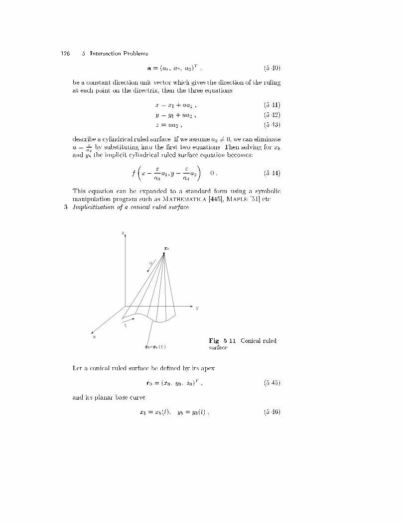
126 5. Intersection Problems
a = (a1; a2; a3)T ; (5.40)
be a constant direction unit vector which gives the direction of the rulingat each point on the directrix, then the three equations
x = xb + ua1 ; (5.41)
y = yb + ua2 ; (5.42)
z = ua3 ; (5.43)
describe a cylindrical ruled surface. If we assume a3 6= 0, we can eliminateu = z
a3by substituting into the �rst two equations. Then solving for xb
and yb the implicit cylindrical ruled surface equation becomes:
f
�x� z
a3a1; y � z
a3a2
�= 0 : (5.44)
This equation can be expanded to a standard form using a symbolicmanipulation program such as Mathematica [445], Maple [51] etc.
3. Implicitization of a conical ruled surface
x
z
y
u
t
rb=rb(t)
r0
Fig. 5.11. Conical ruledsurface
Let a conical ruled surface be de�ned by its apex
r0 = (x0; y0; z0)T ; (5.45)
and its planar base curve
xb = xb(t); yb = yb(t) ; (5.46)

5.5 Point/surface intersection 127
which is a degree n planar rational polynomial curve on the xy plane. Itsimplicit equation
f(xb; yb) = 0 ; (5.47)
is a total degree n polynomial. The equation of the resulting conical ruledsurface is
x = x0(1� u) + xbu ; (5.48)
y = y0(1� u) + ybu ; (5.49)
z = z0(1� u) : (5.50)
Eliminating u by substituting u = 1 � zz0
into (5.48) and (5.49), wherewe assume z 6= z0, and solving for xb; yb yields:
f
�z0
z0 � z x�x0
z0 � z z;z0
z0 � z y �y0
z0 � z z�= 0 : (5.51)
This equation can be expanded to the standard form using a symbolicmanipulation program such as Mathematica [445], Maple [51] etc.
Newton's method. We start with preprocessing using the bounding boxof the RPP surface patch coupled with some level of subdivision. Then wesolve a system x0 = x(u; v), y0 = y(u; v) using Newton's method and verifythe results with the third equation z0 = z(u; v). Projection of r0 onto aplanar approximation of the surface (faceting) may provide a good initialapproximation.
Bounding box and subdivision followed by minimization method.We can easily extend the point/curve intersection case to the point/surfaceintersection case.
Distance function method. Similarly to the point/curve intersection case,detailed formulation of the squared distance function between a point and arational polynomial parametric surface is given in Chap. 7, and the solutionmethod is provided in Chap. 4.
5.5.3 Point/procedural parametric surface intersection
Procedural surfaces may include o�set surfaces, generalized cylinder surfaces,blending surfaces etc. The typical solution method is minimization [69]. Inthis case, no convex box assistance is available in general, and we need adense sampling for an initial approximation which may be expensive, and norigorous guarantees for the solution's reliability are generally available.
For certain classes of procedural surfaces such as o�sets and evolutes ofrational surfaces involving radicals of polynomials, it is possible to use theauxiliary variable method, described in Sect. 4.5, to remove radicals from the

128 5. Intersection Problems
formulation, followed by solution via the IPP algorithm of Chap. 4. Alterna-tively, some procedural surfaces admit a rational parametrization (e.g. o�sets[239, 323], pipe and canal surfaces [240, 255]) in which case the problem re-duces to the formulation of Sect. 5.5.2.
5.6 Curve/curve intersection
Curve to curve intersection cases are identi�ed in Table 5.1. Conceptually,case D3 (RPP/IA curve intersections) is the simplest of the above cases ofintersection to describe and use for illustrating various general di�culties ofintersection problems (see Sect. 5.6.1). The next case of interest is case D1(RPP/RPP curve intersections) from Table 5.1 and this is analyzed in Sect.5.6.2. Next cases D2 and D5 (RPP/PP and PP/PP curve intersections) fromTable 5.1 are analyzed in Sect. 5.6.3. These are followed by cases D6 (PP/IAcurve intersections) and D8 (IA/IA curve intersections) analyzed in Sects.5.6.4 and 5.6.5, respectively. Cases D4, D7, D9 and D10 are not addressedhere, however the reader should be able to analyze those cases based on thecases treated in this section.
Table 5.1. Classi�cation of curve/curve intersections
Curve typeCurve type RPP PP IA IP
RPP D1 D2 D3 D4PP D5 D6 D7IA D8 D9IP D10
5.6.1 Rational polynomial parametric/implicit algebraic curveintersection (Case D3)
2-D planar case. We start with an intersection problem of a planar RPPcurve and an implicit algebraic curve which is de�ned as:
r = r(t) =
�X(t)
W (t);Y (t)
W (t)
�T\ f(x; y) = 0; 0 � t � 1 : (5.52)
Let us denote the degree of planar RPP curve by n and the total degreeof the implicit algebraic curve by m. Furthermore we describe the implicitcurve by
f(x; y) =
mXi=0
m�iXj=0
cijxiyj = 0 : (5.53)

5.6 Curve/curve intersection 129
Substitution of x = X(t)W (t) and y = Y (t)
W (t) into the implicit form and multipli-
cation of Wm(t) leads to a polynomial of degree up to mn
F (t) =mXi=0
m�iXj=0
cijXi(t)Y j(t)Wm�i�j(t) =
mnXi=0
aiti = 0 : (5.54)
Therefore the problem of intersection is equivalent to �nding the realroots of F (t) in 0 � t � 1. The most usual form of F (t) is the power basis.The coe�cients can be evaluated symbolically by substitution and collectionof terms. This can be readily done in a standard symbolic manipulationprogram such as Mathematica [445], Maple [51] etc. This can be followedby numerical evaluation of the coe�cients ideally in exact rational arithmetic.Symbolic manipulation programs are oriented to processing rational numbersexactly.
Example 5.6.1. Let the algebraic curve be an ellipse x2
4 +y2�1 = 0, and theparametric curve be a cubic B�ezier curve with control points (0,1), (1, -4),(2,1) and (2,0) as illustrated in Fig. 5.12. The ellipse and B�ezier curve arechosen to be tangent at (2,0).
Using a symbolic manipulation program and simplifying, we get in exactarithmetic mode:
F (t) = 1025t6 � 3840t5 + 5514t4 � 3728t3 + 1149t2 � 120t = 0 :
Next we �nd the real roots of F (t) in t 2 [0; 1] using factoring over theintegers, which leads to
F (t) � t(t� 1)2G(t) ;
where
G(t) = 1025t3 � 1790t2 + 909t� 120 :
Using a standard numerical solver for polynomials in oating point suchas [134, 135], we obtain the following numbers as solutions of G(t) = 0
t = 0:9228 � � � ; 0:61843 � � � ; 0:2051 � � � :
Alternately solving F (t) = 0 using the same routine leads to the followingsix complex and real roots
tR 1 1 0:9228 0:6183 0:2051 0tI �0:22� 10�6 0:22� 10�6 0 0 0 0
where t = tR + itI , and i is the imaginary unit.

130 5. Intersection Problems
x
2
y
1
Fig. 5.12. Intersection of ellipseand cubic B�ezier curve
Notice the sensitivity to errors for the 6th degree polynomial, especiallyfor the double root t = 1. In oating point arithmetic, such roots may splitinto conjugate complex numbers. Obviously, complex roots are not usable aswe require only the real intersection points. The consequence is lost roots,which implies an erroneous solution of the intersection problem.
An alternate basis for the representation of F (t) = 0 is the Bernsteinbasis, which leads to better stability for its real roots under perturbations ofits coe�cients than the power form [105] as we discussed in Sect. 1.3.3.
Setting F (t) =P6
i=0 ciBi;6(t) in the above example of the ellipse andcubic B�ezier curve, we have c0 = 0, c1 = -20, c2 =
18350 , c3 = � 83
50 , c4 =85 , c5
= 0, and c6 = 0. Here the conversion is done exactly using rational arithmetic(given that the conversion itself is not in general numerically well conditioned[106]). By the use of linear precision property
t =
mnXi=0
i
mnBi;mn(t) ; (5.55)
we can construct a graph
f(t) = (t; F (t))T =mnXi=0
�imnci
�Bi;mn(t) ; (5.56)

5.6 Curve/curve intersection 131
which is now a degree mn B�ezier curve as shown in Fig. 5.13. Now we canapply the IPP method introduced in Chap. 4 which converts the problem of�nding roots of polynomials into a problem of �nding the intersection of theB�ezier curve with the parameter axis.
t1
F(t)
0
Fig. 5.13. Intersection of a B�ezier curve/straight line
Notice that in our example c0 = 0 which implies that t = 0 is a root. Alsoc5 = c6 = 0 implies that t = 1 is a double root.
3-D space curve. The intersection problem of a 3-D rational polynomialparametric curve and a 3-D implicit curve is de�ned as:
r = r(t) =
�X(t)
W (t);Y (t)
W (t);Z(t)
W (t)
�T\ f(r) = g(r) = 0; 0 � t � 1 :
(5.57)
If we denote the total degree of implicit algebraic surfaces f(x; y; z) = 0
and g(x; y; z) = 0 as m, and substituting x = X(t)W (t) , y = Y (t)
W (t) and z = Z(t)W (t)

132 5. Intersection Problems
into the implicit forms f(x; y; z) = 0 and g(x; y; z) = 0 and multiplying byWm(t), we obtain two univariate nonlinear polynomial equations F1(t) = 0and F2(t) = 0. One way to solve this problem is to compute the resultant ofF1(t), F2(t), where all the coe�cients of the two polynomials are known. Ifthe resultant R(F1(t); F2(t)) � 0, then there is a common root between thetwo polynomials and hence we can use the inversion algorithm to �nd t.
A robust way to solve this overconstrained problem F1(t) = F2(t) = 0 (2equations with 1 unknown) is to use the IPP algorithm (see Chap. 4). In suchcases, the substitution must be conducted in exact arithmetic, to maintain apristine or guaranteed precision statement of the problem.
Alternatively one could directly solve the overconstrained �ve-equationsystem in four variables (x, y, z, t)
X(t)� x W (t) = 0 ; (5.58)
Y (t)� y W (t) = 0 ; (5.59)
Z(t)� z W (t) = 0 ; (5.60)
f(x; y; z) = 0 ; (5.61)
g(x; y; z) = 0 ; (5.62)
using the IPP algorithm as in Chap. 4.
5.6.2 Rational polynomial parametric/rational polynomialparametric curve intersection (Case D1)
We can de�ne the intersection problem as:
r = r1(t) =
�X1(t)
W1(t);Y1(t)
W1(t);Z1(t)
W1(t)
�T; 0 � t;� 1 ; (5.63)
\ r = r2(�) =
�X2(�)
W2(�);Y2(�)
W2(�);Z2(�)
W2(�)
�T; 0 � � � 1 :
Setting r1(t) = r2(�) leads to 3 nonlinear polynomial equations with 2unknowns t, � (overconstrained system). There are several approaches tosolve this intersection problem.
1. The bounding box and subdivision method followed by minimization thatwe described in Sect. 5.4.2 can be applied to this problem. If two bound-ing boxes intersect, and they are of �nite size, we can �nd roots usinglinear approximation. However, in the presence of tangential intersectionthe following cases may happen. The boxes intersect but the linear ap-proximations do not, and the curves intersect as illustrated in Fig. 5.14(a) for planar curves. Similar behavior is observed in (b) where polygonis used as the curve approximation. Hodographs indicate the range of tan-gent directions of a B�ezier curve. Sederberg and Meyers [378] construct a

5.6 Curve/curve intersection 133
bounding wedge, which is a bounding angular sector of a hodograph, con-taining all tangent vectors of the given B�ezier curve (see shaded trianglein Fig. 5.15). The bounding wedges are useful in predicting the number ofintersection points of two curves. We �rst translate the bounding wedgesof the two B�ezier curves so that their vertices are coincident. If the twowedges do not overlap, the curves cannot intersect more than once. Thisis a su�cient condition but not a necessary condition. Figure 5.15 (a)shows non-overlapping wedges, while (b) shows overlapping wedges. Inboth �gures, hodographs together with their control polygons for eachB�ezier curve are superposed on the corresponding wedges.If we combine the bounding box subdivision technique with the boundingwedge technique, we are able to locate the intersection points more ef-fectively. For a precisely tangential intersection, this method would leadto in�nite subdivision steps.
2. Another possible approach is to choose 2 equations to solve for t, �, andthen substitute the results into the third equation for veri�cation. We can
implicitize x = X2(�)W2(�)
and y = Y2(�)W2(�)
to obtain f(x; y) = 0 followed by the
substitution of x = X1(t)W1(t)
and y = Y1(t)W1(t)
into f(x; y) yielding F (t) = 0.
Then solve it for real roots in [0; 1] and use the inversion algorithm to
�nd �. Finally we verify the solution by checking if Z1(t)W1(t)
becomes equal
to Z2(�)W2(�)
. This method needs to be implemented in rational arithmetic
for robustness.3. Hawat and Piegl [156] studied the application of a genetic algorithm to the
curve/curve intersection problems. First a number of points are selectedon each curve in a random manner, then a pair of points from each curveare coupled. Finally the genetic algorithm is applied to create generationsof couples that minimize the distance between them. The probabilisticnature of genetic algorithms is discussed in [266].
4. Solve directly the overconstrained 3-equations with 2-unknowns systemusing the IPP algorithm described in Chap. 4. If the parametric curvesare in integral/rational B-spline form, the �rst step is to subdivide theintegral/rational B-spline curve into a number of integral/rational B�eziercurves. This method guarantees a robust solution (no missing roots).
5.6.3 Rational polynomial parametric/procedural parametric andprocedural parametric/procedural parametric curve intersections(Cases D2 and D5)
These intersection problems are de�ned as:
r = r1(t) \ r = r2(�); 0 � t; � � 1 ; (5.64)
where we have 3 equations with 2 unknowns t and �. Unlike the RPP/RPPcurve intersection, there is no known and easily computable convex box de-creasing arbitrarily with subdivision for PP curves.

134 5. Intersection Problems
(a) (b)
Fig. 5.14. Linear approximation of curves in �nding intersections: (a) approxima-tion by linear segments, (b) approximation by polygon
BBBBBBBBBBBBBBBBBBBBBBBBBBBBBBBBBBBBBBBBBBBBBBBBBBBBBBBBBBBBBBBBBBBBBBBBBBBBBBBBBBBBBBBBBBBBBBBBBBBBBBBBBBBBBBBBBBBBBBBBBBBBBBBBBBBBBBBBBBBBBBB
BBBBBBBBBBBBBBBBBBBBBBBBBBBBBBBBBBBBBBBBBBBBBBBBBBBBBBBBBBBBBBBBBBBBBBBBBBBBBBBBBBBBBBBBBBBBBBBBBBBBBBBBBBBBBBBBBBBBBBBBBBBBBBBBBBBBBBBBBBBBBBBBBBBBBBBBBBBBBBBBBBBBBBBBBBBBBBBBBBBBBBBBBBBBBBBBBBBBBBBBBBBBBBBBBBBBBBBBBBBBBBBBBBBBBBBBBBBBBBBBBBBBBBBBBBBBB
BBBBBBBBBBBBBBBBBBBBBBBBBBBBBBBBBBBBBBBBBBBBBBBBBBBBBBBBBBBBBBBBBBBBBBBBBBBBBBBBBBBBBBBBBBBBBBBBBBBBBBBBBBBBBBBBBBBBBBBBBBBBBBBBBBBBBBBBBBBBBBBBBBBBBBBBBBBBBBBBBBBBBBBB
BBBBBBBBBBBBBBBBBBBBBBBBBBBBBBBBBBBBBBBBBBBBBBBBBBBBBBBBBBBBBBBBBBBBBBBBBBBBBBBBBBBBBBBBBBBBBBBBBBBBBBBBBBBBBB
(a)
(b)
Fig. 5.15. Bounding wedges
A possible approach is to minimize the squared distance function D be-tween RPP curve and PP curve or between two PP curves
D = F (t; �) = jr1(t)� r2(�)j2; 0 � t; � � 1 ; (5.65)
using numerical techniques [69]. Initial approximation may be obtained by us-ing linear approximations of r1(t) and r2(�). In general there is no guaranteeto �nd all the stationary points.

5.6 Curve/curve intersection 135
For o�sets and evolutes of rational polynomial curves, we are able toavoid the square roots of polynomials by using the auxiliary variable method,described in Sect. 4.5, so that we can apply the IPP algorithm to enhancerobustness.
5.6.4 Procedural parametric/implicit algebraic curve intersection(Case D6)
The intersection problem is de�ned as:
r = r(t) \ f(r) = g(r) = 0; 0 � t � 1 : (5.66)
This can be reduced to PP curve/IA surface intersection (see Sect. 5.7.4), i.e.r = r(t) \ f(r) = 0 and r = r(t) \ g(r) = 0, and comparison of solutions.
5.6.5 Implicit algebraic/implicit algebraic curve intersection(Case D8)
The planar case is of interest in processing trimmed patches and the de�nitionof this intersection problem is given as
f(u; v) = 0 \ g(u; v) = 0; 0 � u; v � 1 : (5.67)
Implicitization. We can eliminate v to form the resultant F (u), then solveF (u) = 0 for u and use the inversion algorithm to obtain v.
Example 5.6.2. Let us consider an ellipse and a circle
f =x2
4+ y2 � 1 = 0 ;
g = (x� 1)2 + y2 � 1 = 0 ;
as in Fig. 5.16.First we eliminate y from these two equations. This leads to
3x2 � 8x+ 4 = 0 ;
which has two real roots x = 2 and x = 23 . These lead to y2 = 0 and y2 = 8
9 ,respectively.
However there are possible numerical problems at the tangential inter-section point x = 2; y = 0. Let us assume that due to error � > 0, wehave
x = 2 + " ;
hencey2 = �"(1 + "
4) < 0 :
This implies that y is imaginary and that no real roots exist. This would haveas a consequence missing an intersection solution, leading to a robustnessproblem.

136 5. Intersection Problems
−2.5 −2 −1.5 −1 −0.5 0 0.5 1 1.5 2 2.5
−1.5
−1
−0.5
0
0.5
1
1.5
x
y
Fig. 5.16. Ellipse and circle intersection
Newton's method. After tracing of f(u; v) = 0 and g(u; v) = 0, based onthe technique which will be discussed in Sect. 5.8.1, linear approximation ofeach algebraic curve is available. By �nding intersections of linear approxima-tions and minimum distance points between them, we can initiate a Newton'smethod on the system f = g = 0 or a minimization of F = f2+ g2. However,no general robustness guarantees exist with such method.
Interval Projected Polyhedron solver. A robust and e�cient method isbased on use of the IPP algorithm, described in Chap. 4 for two equationswith two unknowns.
5.7 Curve/surface intersection
Curve to surface intersections are classi�ed in Table 5.2. Such intersectionproblems are useful in solving the more general surface to surface intersectionproblems. When the curve is a straight line, the curve/surface intersection isuseful for
� ray tracing in computer graphics and visualization;� point classi�cation in solid modeling;� procedural surface interrogation.
In Sects. 5.7.1 to 5.7.6 several of the most frequent curve to surface inter-section problem cases E3, E1, E2/E6, E7, E11, E9 are analyzed in some detail.The remaining cases are not analyzed in detail, but the reader should be ableto analyze them via the cases addressed in this section. We will start withcase E3 (RPP curve to IA surface intersection), which is quite representativeof the complexities of this type of problem.

5.7 Curve/surface intersection 137
Table 5.2. Classi�cation of curve/surface intersections
Surface typeCurve type RPP PP IA IP
RPP E1 E2 E3 E4PP E5 E6 E7 E8IA E9 E10 E11 E12IP E13 E14 E15 E16
5.7.1 Rational polynomial parametric curve/implicit algebraicsurface intersection (Case E3)
The intersection problem is de�ned as:
r = r(t) =
�X(t)
W (t);Y (t)
W (t);Z(t)
W (t)
�T\ f(r) = 0; 0 � t � 1 : (5.68)
Let us consider an implicit algebraic surface of total degree m
f(x; y; z) =
mXi=0
m�iXj=0
m�i�jXk=0
cijkxiyjzk = 0 : (5.69)
We substitute x = X(t)W (t) , y =
Y (t)W (t) and z =
Z(t)W (t) of degree n into the implicit
equation and multiply by Wm(t) leading to
F (t) =
mXi=0
m�iXj=0
m�i�jXk=0
cijkXi(t)Y j(t)Zk(t)Wm�i�j�k(t) = 0 ; (5.70)
of degree � mn in t. We then �nd its real roots in [0; 1], as described inSect. 5.6.1.
Alternatively, the problem can be formulated as a nonlinear polynomialsystem of four equations in four unknowns (x, y, z, t) and solved using theIPP algorithm.
5.7.2 Rational polynomial parametric curve/rational polynomialparametric surface intersection (Case E1)
The intersection problem between a rational polynomial parametric curveand a rational polynomial parametric surface is de�ned as:
r = r1(t) =
�X1(t)
W1(t);Y1(t)
W1(t);Z1(t)
W1(t)
�T; 0 � t � 1 ; (5.71)
\ r = r2(u; v) =
�X2(u; v)
W2(u; v);Y2(u; v)
W2(u; v);Z2(u; v)
W2(u; v)
�T; 0 � u; v � 1 :

138 5. Intersection Problems
The equation consists of three nonlinear equations r1(t) = r2(u; v) in threeunknowns t, u, v. A preprocessing step of checking bounding boxes for absenceof intersection is helpful.
Implicitization. Implicitization of r2(u; v) (which is recommended for lowdegree surfaces) reduces this problem to Case E3 described in Sect. 5.7.1.
Bounding box and subdivision followed by minimization method.Use of bounding boxes coupled with recursive subdivision will lead us tosmall bounding boxes which may contain intersection points. Then we use alinear approximations for r1 and r2 to obtain approximate initial solutions,which can be used to initiate a Newton's method on r1(t)� r2(u; v) = 0 or aminimization method on F (t; u; v) = jr1(t)� r2(u; v)j2. However, no generalrobustness guarantees exist with such method.
Interval Projected Polyhedron solver. A robust and e�cient way isto solve the three equations with three unknowns using the IPP algorithmdiscussed in Chap. 4.
5.7.3 Rational polynomial parametric/procedural parametric andprocedural parametric/procedural parametric curve/surfaceintersections (Cases E2/E6)
The intersection problem between a rational polynomial parametric curve ora procedural parametric curve and a procedural parametric surface is de�nedas:
r = r1(t) \ r = r2(u; v); 0 � t; u; v � 1 : (5.72)
Similar to Case E1, this problem reduces to three nonlinear equations inthree unknowns involving non-polynomial functions, for which bounds arenot generally available.
A possible approach is to use the minimization technique
F (t; u; v) = jr1(t)� r2(u; v)j2 ; (5.73)
in a cube 0 � t; u; v � 1. Comments under the point/PP curve intersectioncase (see Sect. 5.4.3) also apply to this problem.
5.7.4 Procedural parametric curve/implicit algebraic surfaceintersection (Case E7)
The intersection problem between a procedural parametric curve and an im-plicit algebraic surface is de�ned as:
r = r(t) \ f(r) = 0; 0 � t � 1 : (5.74)
This leads to four nonlinear equations in four unknowns t, r. We could useNewton's method initiated by a linear approximation of r = r(t), which canbe intersected more easily with f(r) = 0 using the method of Case E3 (seeSect. 5.7.1). However, no robustness guarantees exist in general.

5.8 Surface/surface intersections 139
5.7.5 Implicit algebraic curve/implicit algebraic surfaceintersection (Case E11)
Implicit algebraic curve and implicit algebraic surface intersection problemis de�ned as:
f(r) = g(r)| {z }curve
= h(r)|{z}surface
= 0 : (5.75)
The formulation comprises three nonlinear equations in three unknowns r.Possible solution approaches include elimination methods, Newton's method,minimization methods with objective function F (r) = f2 + g2 + h2, approx-imating f(r) = g(r) = 0 curve with a linear spline reducing to Case E3 andre�nement using minimization, and the IPP algorithm.
5.7.6 Implicit algebraic curve/rational polynomial parametricsurface intersection (Case E9)
The implicit algebraic curve and rational polynomial parametric surface in-tersection is de�ned as:
f(r) = g(r) = 0 \ r = r(u; v) =
�X(u; v)
W (u; v);Y (u; v)
W (u; v);Z(u; v)
W (u; v)
�T;
0 � u; v � 1 : (5.76)
By substituting r = r(u; v) into f(r) = 0 and g(r) = 0 we obtain two algebraiccurves F (u; v) = 0 and G(u; v) = 0. This formulation reduces to IA/IA curveintersection, Case D8 in Sect. 5.6.5 (see Fig. 5.17). A more detailed discussionof algebraic curves is given in Sect. 5.8.1.
5.8 Surface/surface intersections
Surface to surface intersection cases are identi�ed in Table 5.3. The solu-tion of a surface/surface intersection problem may be empty, or include acurve (possibly made of several branches), a surface patch, or a point. InSects. 5.8.1 to 5.8.3 several of the most frequent surface to surface intersec-tion problem cases F3, F1, and F8 are studied in detail. The remaining casesare not analyzed, but could be addressed based on cases F3, F1 and F8,although without general robustness guarantees. Conceptually, RPP/IA sur-face intersection (Case F3) is the simplest of the above cases and may serveas illustrating general di�culties of surface to surface intersection problems.

140 5. Intersection Problems
u
v
G(u,v)=0
F(u,v)=0
Fig. 5.17. Intersection of two al-gebraic curves
Table 5.3. Classi�cation of surface/surface intersections
Surface typeSurface type RPP PP IA IP
RPP F1 F2 F3 F4PP F5 F6 F7IA F8 F9IP F10
5.8.1 Rational polynomial parametric/implicit algebraic surfaceintersection (Case F3)
We start with a rational polynomial parametric surface to implicit algebraicsurface intersection problem de�ned as:
r = r(u; v) =
�X(u; v)
W (u; v);Y (u; v)
W (u; v);Z(u; v)
W (u; v)
�T\ f(r) = 0; 0 � u; v � 1 :
(5.77)
This leads to four algebraic equations in �ve unknowns r; u; v (undercon-strained system). For the usual low degree surfaces f(r) and low degreepatches r(u; v), we can substitute r(u; v) into f(r) = 0 to obtain an im-plicit algebraic curve in u; v [124, 332, 210, 301, 211]. Examples of low orderimplicit algebraic surfaces in practical use are planes (degree 1), the naturalquadrics (cylinder, sphere, cone) (degree 2), and torii (degree 4). In fact ina survey of mechanical parts (mechanical elements), over 90% of all surfacesinvolved are of these types [149]. It is also well known that low order implicitalgebraic surfaces have a low degree rational polynomial parametric repre-sentation (which can be easily obtained [313]), so that when two such low

5.8 Surface/surface intersections 141
order implicit algebraic surfaces are intersected, the methods of this sectionmay be also used.
Formulation. Now let us denote the implicit algebraic surface f(x; y; z) = 0of total degree m by
f(x; y; z) =
mXi=0
m�iXj=0
m�i�jXk=0
cijkxiyjzk : (5.78)
By substituting x = X(u;v)W (u;v) ; y = Y (u;v)
W (u;v) ; z = Z(u;v)W (u;v) , where X(u; v),
Y (u; v), Z(u; v) and W (u; v) are all of maximum degree p in u and q in vinto (5.78) and multiplying by Wm(u; v) leads to an algebraic curve
F (u; v) =
mXi=0
m�iXj=0
m�i�jXk=0
cijkXi(u; v)Y j(u; v)Zk(u; v)Wm�i�j�k(u; v) = 0 ;
(5.79)
of maximum degreeM = mp and N = mq in u; v, respectively. Consequently,the problem of intersection reduces to the problem of tracing F (u; v) = 0without omitting any special features of the curve, e.g. small loops, singu-larities, and accurately computing all its branches. This is a fundamentalproblem in algebraic geometry [436] and much work has been done to un-derstand its solution. In the context of algebraic geometry the coe�cients ofF (u; v) = 0 are integers. In the context of CAD and computer implementa-tion, the coe�cients of F = 0, and r = r(u; v) are oating point numbers.Therefore, if the above substitution is performed in oating point arithmeticthe coe�cients of F (u; v) = 0 involve error, which may considerably modifythe problem being solved. To avoid such error, rational arithmetic may beused for robustness. These issues are discussed in the Chap. 4.
The algebraic curve
F (u; v) =
MXi=0
NXj=0
cMij uivj = 0 ; (5.80)
can be reformulated in terms of Bernstein polynomials using (4.18) as follows:
F (u; v) =
MXi=0
NXj=0
cBijBi;M (u)Bj;N (v) = 0 ; (5.81)
where (u; v) 2 [0; 1]2.As an example, consider a plane in an implicit form
ax+ by + cz + d = 0 ; (5.82)
and a rational B�ezier patch of degree m in u, n in v

142 5. Intersection Problems
border points
singularpoints
u
v
F=Fu=Fv=0
v turning point
F=Fu=0
u turning point
F=Fv=0
loop Fig. 5.18. Parameter spaceof r(u; v) and resultingalgebraic curve F (u; v) = 0
r(u; v) =
Pmi=0
Pnj=0 wijbijBi;m(u)Bj;n(v)Pm
i=0
Pnj=0 wijBi;m(u)Bj;n(v)
; (5.83)
where bij = (xij ; yij ; zij)T and weights wij � 0.
The resulting algebraic curve is of the form of equation (5.81) with
cBij = (axij + byij + czij + d)wij : (5.84)
In fact the power basis form of F (u; v) = 0 need not be computed at all, ifpolynomial arithmetic for Bernstein polynomials, described in Sect. 1.3.2, isused (see also [106]).
The advantage of the Bernstein form is the higher numerical stability ofthe roots in comparison to the power basis and the convex hull property. IfcBij > 0 or cBij < 0 for all i; j, there is no solution and the two surfaces donot intersect. More precisely, the entire algebraic surface f(r) = 0 does notintersect the surface patch r = r(u; v) for (u; v) 2 [0; 1]2. Obviously, whenall cBij = 0 the two surfaces coincide in their entirety. A somewhat complexalgebraic curve F (u; v) = 0 is shown in Fig. 5.18 involving various branches(from border to border), internal loops, and singularities.
Tracing method. Given a point on every branch of an algebraic curve, weare able to trace the curve using di�erential curve properties. The idea is to�nd increments �u and �v such that F (u + �u; v + �v) = 0, when we haveF (u; v) = 0.
Let us Taylor expand F (u; v)

5.8 Surface/surface intersections 143
(u,v)
δu
δvδvL
Correction
F(u,v)=0
P
Q
Fig. 5.19. A zoomed view of an algebraic curve near a point (u; v)
F (u+ �u; v + �v) = F (u; v) + Fu�u+ Fv�v (5.85)
+1
2(Fuu�u
2 + 2Fuv�u�v + Fvv�v2) + � � � :
When Fu and Fv are not both zero or F2u+F
2v > 0, in order to have F (u; v) =
0 and F (u+ �u; v + �v) = 0 to the �rst order approximation, we must have
Fu�u+ Fv�v = 0 ; (5.86)
or
�vL = �FuFv�u ; (5.87)
assuming Fv 6= 0. However, as illustrated in Fig. 5.19 �vL leads to a point Qwhich may be far from the curve F (u; v) = 0. Newton's method on F (u +�u; v) = 0 with initial approximation vI = v + �vL may be used to compute�v with high accuracy and in an e�cient manner. For vertical branches, i.e.when jFv j is very small, we may use �uL = �Fv
Fu�v.
To avoid these special stepping procedures, (5.86) may be rewritten as
Fu _u+ Fv _v = 0 ; (5.88)
where u, v are considered as functions of a parameter t. The solution to thedi�erential equation is given by
_u = �Fv(u; v) ; (5.89)
_v = ��Fu(u; v) ; (5.90)
where � is an arbitrary nonzero factor. For example, � can be chosen toprovide arc length parametrization using the �rst fundamental form (3.13)of the surface as a normalization condition

144 5. Intersection Problems
� = � 1pEF 2
v � 2FFuFv +GF 2u
; (5.91)
where E, F and G are �rst fundamental form coe�cients of the paramet-ric surface evaluated at u, v. Equations (5.89) and (5.90) form a system oftwo �rst order nonlinear di�erential equations which can be solved by theRunge-Kutta or other methods with adaptive step size [69, 126]. For thetracing method to work properly, we must provide all the starting points ofall branches in advance. Step size selection is complex and too large a stepsize may lead to straying or looping [124], as in Fig. 5.20, in the presenceof constrictions where F 2
u + F 2v is very small. Tracing through singularities
(F 2u +F 2
v = 0) is also problematic. When �pF 2u + F 2
v is small then the righthand sides of (5.89) and (5.90) are small and step size needs to be reducedfor topologically reliable tracing of the curve.
straying looping
Fig. 5.20. Step size problems in tracing method
Characteristic points. Starting points for tracing algebraic curves areidenti�ed by looking for characteristic points de�ned below:
1. Border points: The intersections of F (u; v) = 0 with all four boundaryedges of the parameter space [0; 1]2, e.g. F (0; v) = 0; 0 � v � 1.
2. Turning points: The u-turning points are the points where the tangent ofF (u; v) = 0 is parallel to the u = 0 axis, which satis�es the simultaneousequations F = Fv = 0 (with Fu 6= 0). On the other hand the v-turningpoints are the points where the tangent of F (u; v) = 0 is parallel tothe v = 0 axis, which satis�es the simultaneous equations F = Fu = 0(with Fv 6= 0). Both types of turning points are shown in Fig. 5.18. IfF has a degree of (M;N) in (u; v), then the degrees of Fu and Fv will

5.8 Surface/surface intersections 145
be (M � 1; N) and (M;N � 1), respectively. It can be shown that thetotal number of roots of two simultaneous polynomial equations in twovariables whose degrees are (m;n) and (p; q), respectively, ismq+np [95].Therefore the number of u-turning points and v-turning points can beat most 2MN �M and 2MN �N , respectively over the entire complexplane. However within the square parameter space [0; 1]2, the numberof turning points is typically much reduced in practice and thereforemethods that use the [0; 1]2 square as the search space of the roots suchas the IPP algorithm in Sect. 4.9 or interval Newton methods [159] wouldtypically outperform other methods.
3. Singular points: The points on the curve which satisfy the following threesimultaneous equations F = Fu = Fv = 0 are called singular points.Noting that f(x; y; z) = 0, and F (u; v) =Wm(u; v)f(x; y; z), we deduce
Fu = mWm�1Wuf +Wm
�@f
@x
@x
@u+@f
@y
@y
@u+@f
@z
@z
@u
�=Wmrf � ru :
(5.92)
Similarly we obtain Fv =Wmrf � rv , and hence at singular points rf �ru = rf � rv = 0. This means that rf k ru � rv or that the normals oftwo surfaces are parallel and since f(u; v) = 0 at these points the twosurfaces intersect tangentially. If F has a degree of (M;N) in (u; v), thedegrees of Fu and Fv will be (M � 1; N) and (M;N � 1), respectively,thus the number of singular points can be at most 2MN �M �N + 1[95] over the entire complex plane and typically much less in number in[0; 1]2. If the systems F = Fu = 0 and F = Fv = 0 are already solved,a small extra evaluation can identify their common roots which are thesingular points. Alternatively the IPP algorithm for the overconstrainedsystem F = Fu = Fv = 0 can be used to �nd the singular points.
From the above discussions we can get upper bounds for the maximumnumber of u-turning, v-turning and singular points as listed in Table 5.4.These bounds refer to the maximum possible number of solutions (u; v) in theentire complex plane. Biquadratic and bicubic surfaces in the �rst column ofTable 5.4 are degree 8 and 18 implicit algebraic surfaces. It turns out that thenumber of such points in the real square [0; 1]2 is much smaller, but can stillbe quite large. Consequently, methods which focus only on the real solutionsin [0; 1]2 are advantageous, such as IPP algorithm described in Chap. 4 orinterval Newton's method [159].
Analysis of singular points. Let us construct a parametric equation of astraight line L through a point (u0; v0) on the algebraic curve F (u; v) = 0
u = u0 + �t; v = v0 + �t ; (5.93)
where � and � are constants and t is a parameter [436, 95, 107]. We �nd theintersections between L and the algebraic curve F (u; v) = 0 by determining

146 5. Intersection Problems
Table 5.4. Maximum number of turning and singular points in various cases
algebraic max max maxcurve number number number
S1 S2 F (u; v) u-turning v-turning singulardegree pts pts pointsM;N 2MN �M 2MN �N 2MN �M
�N + 1plane biquadratic 2, 2 6 6 5plane bicubic 3, 3 15 15 13quadric biquadratic 4, 4 28 28 25quadric bicubic 6, 6 66 66 61torus biquadratic 8, 8 120 120 113torus bicubic 12, 12 276 276 265
biquadratic biquadratic 16, 16 496 496 481bicubic biquadratic 36, 36 2556 2556 2521bicubic bicubic 54, 54 5778 5778 5725
the roots of F (u0 + �t; v0 + �t) = 0. Since F (u0; v0) = 0, Taylor expansionof the left hand side gives
(�Fu + �Fv)t+1
2(�2Fuu + 2��Fuv + �2Fvv)t
2 + � � � = 0 ; (5.94)
where partial derivatives of F are evaluated at (u0; v0).When Fu and Fv are not both zero (F 2
u + F 2v > 0) at (u0; v0), (5.94) has
a simple root t = 0 and every line through (u0; v0) has a single intersectionwith the algebraic curve at (u0; v0) except for one case where �Fu+�Fv = 0for certain values of � and �. In such cases (5.94) has a double root t =0, provided at least one of the second order partial derivatives is not zero(F 2
uu + F 2uv + F 2
vv > 0), and L is tangent to the curve at (u0; v0).When (u0; v0) is a singular point (Fu(u0; v0) = Fv(u0; v0) = F (u0; v0) =
0), and at least one of Fuu, Fuv , Fvv is not zero (F 2uu + F 2
uv + F 2vv > 0), then
t = 0 is a double root and has at least two intersections at (u0; v0) except forthe values of � and � which satisfy
�2Fuu + 2��Fuv + �2Fvv = 0 : (5.95)
In such cases, t = 0 is a triple root, provided at least one of the third orderpartial derivatives is not zero (F 2
uuu +F2uuv +F
2uvv +F
2vvv > 0). We can solve
the quadratic equation (5.95) for �� or �
� which leads to the following threepossibilities:
(1) Two real distinct roots: These values correspond to two distinct tangentdirections at the singular point, which implies the algebraic curve has aself-intersection. The Folium of Descartes, which is shown in Fig. 1.1, hassuch singularity at the origin.
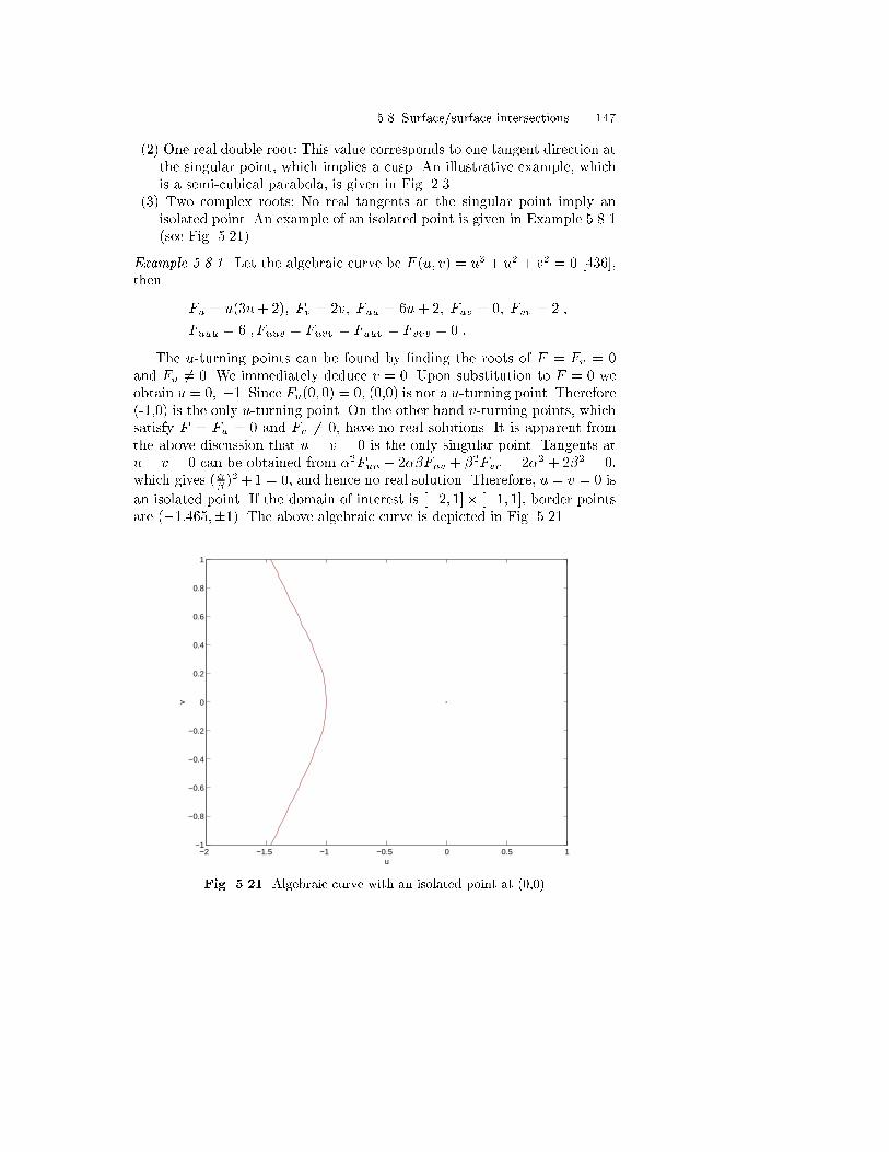
5.8 Surface/surface intersections 147
(2) One real double root: This value corresponds to one tangent direction atthe singular point, which implies a cusp. An illustrative example, whichis a semi-cubical parabola, is given in Fig. 2.3.
(3) Two complex roots: No real tangents at the singular point imply anisolated point. An example of an isolated point is given in Example 5.8.1(see Fig. 5.21).
Example 5.8.1. Let the algebraic curve be F (u; v) = u3 + u2 + v2 = 0 [436],then
Fu = u(3u+ 2); Fv = 2v; Fuu = 6u+ 2; Fuv = 0; Fvv = 2 ;
Fuuu = 6 ; Fuuv = Fuvv = Fuuv = Fvvv = 0 :
The u-turning points can be found by �nding the roots of F = Fv = 0and Fu 6= 0. We immediately deduce v = 0. Upon substitution to F = 0 weobtain u = 0; �1. Since Fu(0; 0) = 0, (0,0) is not a u-turning point. Therefore(-1,0) is the only u-turning point. On the other hand v-turning points, whichsatisfy F = Fu = 0 and Fv 6= 0, have no real solutions. It is apparent fromthe above discussion that u = v = 0 is the only singular point. Tangents atu = v = 0 can be obtained from �2Fuu + 2��Fuv + �2Fvv = 2�2 + 2�2 = 0,which gives (�� )
2+1 = 0, and hence no real solution. Therefore, u = v = 0 is
an isolated point. If the domain of interest is [�2; 1]� [�1; 1], border pointsare (�1:465;�1). The above algebraic curve is depicted in Fig. 5.21.
−2 −1.5 −1 −0.5 0 0.5 1−1
−0.8
−0.6
−0.4
−0.2
0
0.2
0.4
0.6
0.8
1
u
v
Fig. 5.21. Algebraic curve with an isolated point at (0,0)

148 5. Intersection Problems
Example 5.8.2. We have studied the semi-cubical parabola F (u; v) = u3 �v2 = 0 in Example 2.1.1. The curve has a singular point at u = v = 0. Since
Fu = 3u2; Fv = �2v; Fuu = 6u; Fuv = 0; Fvv = �2 ;Fuuu = 6 ; Fuuv = Fuvv = Fuuv = Fvvv = 0 ;
we have �2Fuu + 2��Fuv + �2Fvv = 6u�2 � 2�2 = 0. At (0,0) we have adouble root � = 0. Thus, at the singular point (0,0) we have a cusp whosetangent direction is along the v = 0 axis as shown in Fig. 2.3.
Example 5.8.3. Let us consider the equation
F (u; v) = (u+ 1)u(u� 1)(v + 1)v(v � 1) +1
20= 0 ;
within the domain [�2; 2]2, taken from Geisow [124]. This is a degree 6 alge-braic curve illustrated in Fig. 5.22. On every border line segment, there arethree border points. The curve has no singular points, but involves two (inter-nal) loops and six border-to-border branches. The algebraic curve F (u; v) = 0in this example has degrees M = 3; N = 3 in u and v. Consequently, usingthe previous formulae the number of u turning points, v turning points andsingular points (in the entire complex plane) is bounded by 2MN �M = 15,2MN � N = 15, and 2MN �M �N + 1 = 13. However, as we can see inFig. 5.22, these numbers overestimate the actual number of such points inthe real square [�2; 2]2.Computing starting points for all branches. Starting points for tracingalgebraic curves could be border points, turning points and singular points.Border points involve solution of a univariate polynomial equation, e.g. forborder along u = 0, using (5.81)
F (0; v) =
NXj=0
cB0jBj;N (v) = 0 : (5.96)
Turning and singular point computation involve the �rst order partialderivatives:
Fu(u; v) = M
M�1Xi=0
NXj=0
(cBi+1;j � cBij)Bi;M�1(u)Bj;N (v) ; (5.97)
Fv(u; v) = NMXi=0
N�1Xj=0
(cBi;j+1 � cBij)Bi;M (u)Bj;N�1(v) : (5.98)
Consequently, computation of turning points (F = Fu = 0 and F = Fv = 0)is equivalent to solving a system of two nonlinear polynomial equations in twovariables, and computation of singularities F = Fu = Fv = 0 is equivalent tosolving an overconstrained system of three nonlinear polynomial equationsin two variables. Robust and e�cient solution of these systems of nonlinearpolynomial equations is addressed in Chap. 4.

5.8 Surface/surface intersections 149
−2 −1.5 −1 −0.5 0 0.5 1 1.5 2−2
−1.5
−1
−0.5
0
0.5
1
1.5
2
Fig. 5.22. A degree six algebraic curve (adapted from [124])
5.8.2 Rational polynomial parametric/rational polynomialparametric surface intersection (Case F1)
Rational polynomial parametric surface to rational polynomial parametricsurface intersection is de�ned as:
r = r1(�; t) =
�X1(�; t)
W1(�; t);Y1(�; t)
W1(�; t);Z1(�; t)
W1(�; t)
�T; 0 � �; t � 1 ; (5.99)
\ r = r2(u; v) =
�X2(u; v)
W2(u; v);Y2(u; v)
W2(u; v);Z2(u; v)
W2(u; v)
�T; 0 � u; v � 1 :
Formulation can be provided by setting r1(�; t) = r2(u; v) which leads tothree nonlinear polynomial equations for four unknowns �; t; u; v. It is anunderconstrained system with 3 equations and 4 unknowns. This system canbe solved by the IPP algorithm of Chap. 4. However, as the solutions aretypically not isolated points but curves, such approach is very slow whensmall tolerances are used. One could also implicitize r1(�; t) to the form
f(x; y; z) = 0 and substitute x = X2(u;v)W2(u;v)
, y = Y2(u;v)W2(u;v)
and z = Z2(u;v)W2(u;v)
into
f to reduce the problem to Case F3 for low degree surfaces [211]. Heo et al.[160] studied the intersection of two ruled surfaces which is simpler than thegeneral parametric surface to surface intersection problem.
150 5. Intersection Problems
There are three major techniques for solving RPR/RPP surface intersec-tions. Detailed reviews can be found in [294, 299].
Lattice methods. Lattice method reduces the dimensionality of surface in-tersections by computing intersections of a number of iso-parametric curvesof one surface with the other surface followed by connection of the result-ing discrete intersection points to form di�erent solution branches [351]. Forintersections of parametric patches, the method reduces to the solution ofa large number of independent systems of nonlinear equations. The reduc-tion of problem dimensionality in lattice methods involves an initial choiceof grid resolution, which, in turn, may lead the method to miss importantfeatures of the solution, such as small loops and isolated points which re ectnear tangency or tangency of intersecting surfaces, and to provide incorrectconnectivity. Appropriate methods for the solution of the resulting nonlinearequations in the present context are identi�ed in Chap. 4.
Subdivision methods. Subdivision methods in their most basic form, in-volve recursive decomposition of the problem into simpler similar problemsuntil a level of simplicity is reached, which allows simple direct solution, (e.g.plane/plane intersection [177, 294]). This is followed by a connection phaseof the individual solutions to form the complete solution. Dokken [77] trans-forms surface/surface intersection problems to �nding zeroes of functions offour variables using recursive subdivision techniques [220]. Initially conceivedin the context of intersections of polynomial parametric surfaces [219], theycan be extended to the computation of RPP/IA and IA/IA surface inter-sections [301]. A simple subdivision algorithm employs uniform subdivisionwhich leads to a uniform quadtree data structure shown in Fig. 5.23. Sub-division techniques do not require starting points as marching methods, animportant advantage. General non-uniform subdivision allows selective re-�nement of the solution providing the basis for an adaptive intersection tech-nique. A disadvantage of subdivision techniques used in the evaluation of theentire intersection set is that, in actual implementations with �nite subdivi-sion steps, correct connectivity of solution branches in the vicinity of singularor near-singular points is di�cult to guarantee, small loops may be missed (inmethods with polyhedral surface approximations) or extraneous loops maybe present in the approximation of the solution. Furthermore, if subdivisionmethods are used for high precision evaluation of the entire intersection set,they lead to data proliferation and are consequently slow, and, therefore,unattractive. There are many applications in CAD/CAM, that require highaccuracy, for which pure subdivision methods are impractical. However, adap-tive subdivision methods coupled with e�cient local techniques to get highaccuracy, o�er the best known practical approach for the computation of sig-ni�cant points. These points can then be used in initiating e�cient marchingmethods for tracing intersection curves.
Marching methods. Marching methods involve generation of sequences ofpoints of an intersection curve branch by stepping from a given point on

5.8 Surface/surface intersections 151
BBBBBBBBBBBBBBBBBBBBBBBBBBBBBBBBBBBBBBBBBBBBBBBBBBBBBBBBBBBBBBBBBBBBBBBBBBBBBBBBBBBBBBBBBBBBBBBBBBBBBBBBBBBBBBBBBBBBBBBBBBBBBBBBBBBBBBBBBBBBBBBBBBBBBBBBBBBBBBBBBBBBBBBBBBBBBBBBBBBB
@@@@@@@@@@@@@@@@@@@@@@@@@@@@@@@@@@@@@@@@@@@@@@@@@@@@@@@@
@@@@@@@@@@@@@@@@@@@@@@@@@
@@@@@@@@@@@@@@@@@@@@@@@@@@@@@@
@@@@@@@@@@@@@@@@@@@@@@@@@@@@@@@@@@@@@@@@@@@@@@@@@@@@@@@@
@@@@
Quadtree
@@@@@@
@@@@@@
@@@@@@
@@@@@@@@@
Fig. 5.23. Subdivision method
the required curve in a direction prescribed by the local di�erential geometry[17, 19, 20, 209, 453], as we have studied in tracing the planar algebraic curveF (u; v) = 0 in Sect. 5.8.1. However, such methods are by themselves incom-plete in that they require starting points for every branch of the solution. Inorder to identify all connected components of the intersection curve, a set ofimportant points on the intersection curve (signi�cant points) can be de�ned.As seen in Sect. 5.8.1, such a set may include border, turning and singularpoints of the intersection and provides at least one point on any connectedintersection segment and identi�es all singularities. For a 3-D RPP/RPP in-tersection case a more convenient set of such points su�cient to discover allconnected components of the intersection, includes border and collinear nor-mal points between the two surfaces. Collinear normal points provide pointsinside all intersection loops and all singular points.
Border points are points of the intersection at which at least one of theparametric variables �; t; u; v takes a value equal to the border of the �-tor u-v parametric domain. To compute border points, a piecewise rationalpolynomial curve to piecewise rational polynomial surface intersection capa-bility is required, e.g., r1(0; t) = r2(u; v), which we discussed in Sect. 5.7.2.M�ullenheim [277] addressed a local method to �nd starting points for twoparametric surfaces. Abdel-Malek and Yeh [1] introduced two local meth-ods, iterative optimization and the Moore-Penrose pseudo-inverse method to

152 5. Intersection Problems
determine starting points on the intersection curve between two parametricsurfaces.
Sederberg et al. [375] �rst recognized the importance of collinear normalpoints in detecting the existence of closed intersection loops in intersectionproblems of two distinct parametric surface patches. These are points on thetwo parametric surfaces at which the normal vectors are collinear. Collinearnormal points are a subset of parallel normal points �rst used by Sinha et al.[395] in surface intersection loop detection methods.
To simplify the notation, we replace r1(�; t) by p(�; t) and r2(u; v) byq(u; v). Then the collinear normal points satisfy the following equations [375]
(p� � pt) � qu = 0; (p� � pt) � qv = 0 ;
(p� q) � p� = 0; (p� q) � pt = 0 : (5.100)
Equations (5.100) form a system of four nonlinear polynomial equationsthat can be solved using the robust methods of Chap. 4. Now we split thepatches in (at least) one parametric direction at these collinear normal points.Consequently, starting points are only border points on the boundaries of allsubdomains created. Grandine and Klein [133] follow a systematic approachfor topology resolution of B-spline surface intersections. In this process, theydetermine the structure of the intersection curves including closed loops priorto numerical tracing (following a marching method based on numerical inte-gration of a di�erential algebraic system of equations). Topology resolution inthis context relies on an extension of the PP algorithm (see Sect. 4.4) to the B-spline case implemented in oating point (with normalization of the equationsin the range [-1,1] and normalization of the knot vector in each subdomain inthe range [0,1] at each iteration step of the process to capitalize on the higherdensity of oating point numbers in this range, thereby improving numericalrobustness of the algorithm). An alternate way to detect closed intersectionloops is to use topological methods [235, 53, 263, 209, 244, 243, 435, 434]. Alsobounding pyramids [208, 381] can be used e�ectively to assure the nonexis-tence of closed surface to surface intersection loops. These earlier methodsneed to be implemented in exact or RIA for robustness.
In order to trace the intersection curve, starting points must be locatedprior to tracing. An intersection curve branch can be traced if its pre-imagestarts from the parametric domain boundary in either parameter domain[19]. The marching direction coincides with the tangential direction of theintersection curve c(s) which is perpendicular to the normal vectors of bothsurfaces. Therefore, the marching direction can be obtained as follows:
c0(s) =P(�; t) �Q(u; v)
jP(�; t) �Q(u; v)j ; (5.101)
where the normalization forces c(s) to be arc length parametrized and
P(�; t) = p� � pt; Q(u; v) = qu � qv ; (5.102)

5.8 Surface/surface intersections 153
are the normal vectors of p and q, respectively. When the two surfaces in-tersect tangentially, we cannot use (5.101) since the denominator vanishes.In such cases we must �nd the marching direction in an alternate way whichwill be discussed in Sect. 6.4.
The intersection curve can also be viewed as a curve on the two inter-secting surfaces. A curve � = �(s), t = t(s) in the �t-plane de�nes a curver = c(s) = p(�(s); t(s)) on a parametric surface p(�; t), as well as a curveu = u(s) v = v(s) in the uv-plane de�nes a curve r = c(s) = q(u(s); v(s))on a parametric surface q(u; v). We can derive the �rst derivative of theintersection curve as a curve on the parametric surface using the chain rule:
c0(s) = p��0 + ptt
0; c0(s) = quu0 + qvv
0 : (5.103)
Since we know the unit tangent vector of the intersection curve from(5.101), we can �nd �0 and t0 as well as u0 and v0 by taking the dot producton both hand sides of the �rst equation of (5.103) with p� and pt and thesecond equation with qu and qv , which leads to two linear systems [178]. Thesolutions are immediately obtained as
�0 =det(c0;pt;P(�; t))P(�; t) �P(�; t) ; t0 =
det(p� ; c0;P(�; t))
P(�; t) �P(�; t) ; (5.104)
u0 =det(c0;qv;Q(u; v))
Q(u; v) �Q(u; v); v0 =
det(qu; c0;Q(u; v))
Q(u; v) �Q(u; v); (5.105)
where det denotes the determinant.The points of the intersection curves are computed successively by inte-
grating the initial value problem for a system of nonlinear ordinary di�erentialequations (5.104) and (5.105) using numerical techniques such as the Runge-Kutta or adaptive stepping methods [69, 126]. Figure 5.24 presents the inter-section of a rational quadratic-linear B-spline patch (representing a cylinder)with a biquadratic B�ezier patch representing an elliptic paraboloid [207].Figure 5.25 presents the intersection between two biquartic B�ezier patches(nearly coincident surfaces) [209].
5.8.3 Implicit algebraic/implicit algebraic surface intersection(Case F8)
Implicit algebraic surface to implicit algebraic surface intersection is de�nedas follows:
f(r) = 0 \ g(r) = 0 ; (5.106)
where f; g are polynomial functions. Here we have two equations in threeunknowns r. Bajaj et al. [17] developed a marching method for IA/IA surfaceintersection as well as for parametric surfaces.

154 5. Intersection Problems
Fig. 5.24. Cylinder - elliptic paraboloid intersection (adapted from [207])
Fig. 5.25. Intersection of two biquartic B�ezier patches forming four small loops(adapted from [209])
A method for low order f , g is to eliminate one variable (e.g. z) to �ndprojection of intersection curves on the plane of other two variables (e.g. x,y), then trace the algebraic curve and use the inversion algorithm to �nd z.Intersections of low degree implicit algebraic surfaces are of special interestin the boundary evaluation of the Constructive Solid Geometry models. Amore complete analysis of the special intersections of two quadric surfaces

5.8 Surface/surface intersections 155
(used frequently in CAD/CAM of mechanical parts) can be found in [232,233, 366, 104, 442, 389, 267].
Example 5.8.4. Consider the intersection of a sphere and a circular cylindergiven by
f = x2 + y2 + z2 � 1 = 0 ;
g = x2 + (y � 1
2)2 � 1
4= 0 ;
as shown in Fig. 5.26. The projection of the intersection curves on the threecoordinate planes is illustrated in Fig. 5.27.
Hartmann [155] proposed the idea of numerical implicitization which al-lows treatment of intersection problems of not only parametric surfaces butalso non-standard surfaces such as an o�set of an implicit surface, a Voronoisurface, an envelope of a one parametric family of spheres etc. The key ideais that in tracing the intersection curve of two implicit surfaces, we are onlyrequired to calculate the implicit function values and the gradients of theimplicit functions at the intersection points as in Bajaj et al. [17]. In otherwords, we do not need to know the functions explicitly. Therefore if we canimplicitize any two surfaces numerically we are able to trace the intersectioncurve using the IA/IA surface intersection algorithm of Bajaj et al. [17].
Fig. 5.26. Intersection of two implicit quadrics (sphere and cylinder)

156 5. Intersection Problems
−1.5 −1 −0.5 0 0.5 1 1.5−1.5
−1
−0.5
0
0.5
1
1.5
x
y
(a)
−1.5 −1 −0.5 0 0.5 1 1.5
−1
−0.5
0
0.5
1
y
z
(b)
−1.5 −1 −0.5 0 0.5 1 1.5−1.5
−1
−0.5
0
0.5
1
1.5
x
z
(c)
Fig. 5.27. (a) Projection of intersection curve on z = 0 (xy) plane, i.e. x2 + (y �12)2� 1
4= 0, (b) projection of intersection curve on x = 0 (yz) plane, i.e. y = 1�z2,
(c) projection of intersection curve on y = 0 (xz) plane, i.e. x2 + z4 � z2 = 0
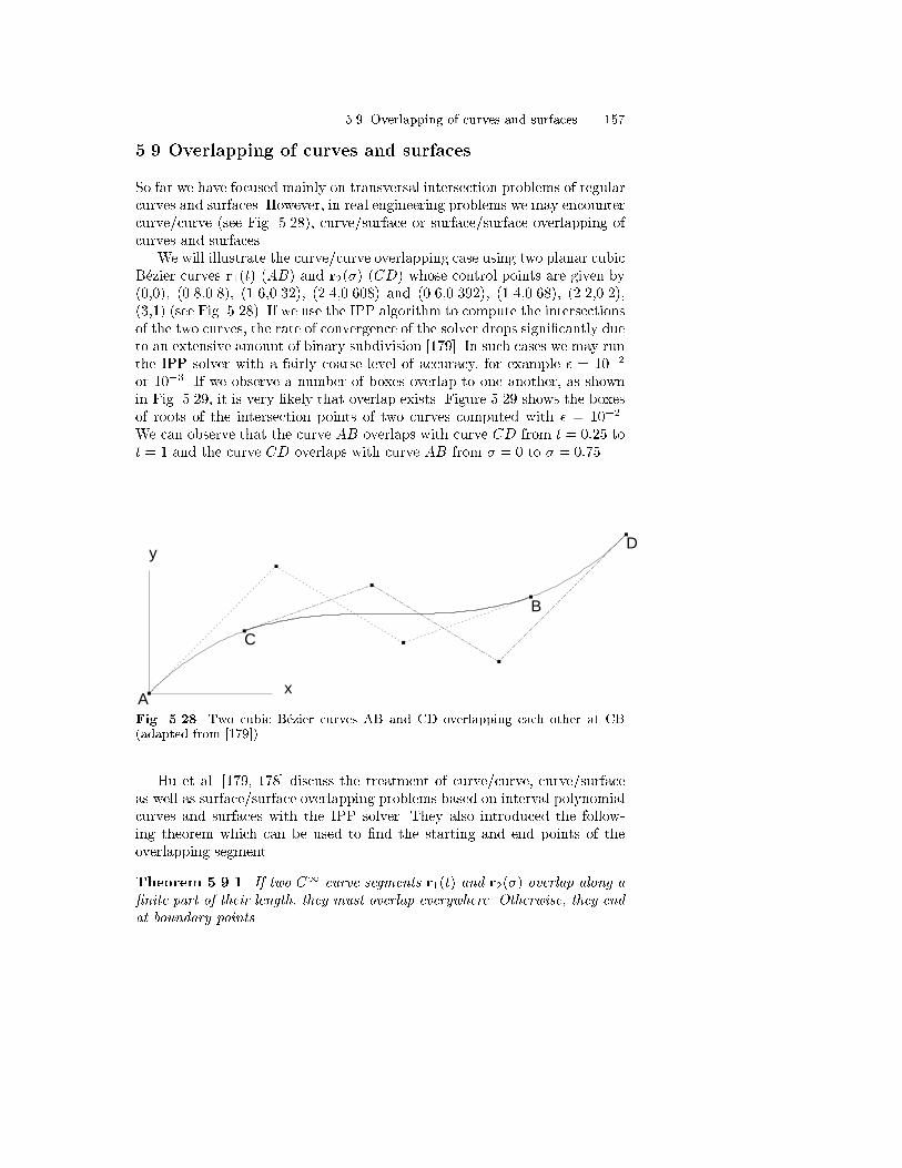
5.9 Overlapping of curves and surfaces 157
5.9 Overlapping of curves and surfaces
So far we have focused mainly on transversal intersection problems of regularcurves and surfaces. However, in real engineering problems we may encountercurve/curve (see Fig. 5.28), curve/surface or surface/surface overlapping ofcurves and surfaces.
We will illustrate the curve/curve overlapping case using two planar cubicB�ezier curves r1(t) (AB) and r2(�) (CD) whose control points are given by(0,0), (0.8,0.8), (1.6,0.32), (2.4,0.608) and (0.6,0.392), (1.4,0.68), (2.2,0.2),(3,1) (see Fig. 5.28). If we use the IPP algorithm to compute the intersectionsof the two curves, the rate of convergence of the solver drops signi�cantly dueto an extensive amount of binary subdivision [179]. In such cases we may runthe IPP solver with a fairly coarse level of accuracy, for example � = 10�2
or 10�3. If we observe a number of boxes overlap to one another, as shownin Fig. 5.29, it is very likely that overlap exists. Figure 5.29 shows the boxesof roots of the intersection points of two curves computed with � = 10�2.We can observe that the curve AB overlaps with curve CD from t = 0:25 tot = 1 and the curve CD overlaps with curve AB from � = 0 to � = 0:75.
x
y
A
B
C
D
Fig. 5.28. Two cubic B�ezier curves AB and CD overlapping each other at CB(adapted from [179])
Hu et al. [179, 178] discuss the treatment of curve/curve, curve/surfaceas well as surface/surface overlapping problems based on interval polynomialcurves and surfaces with the IPP solver. They also introduced the follow-ing theorem which can be used to �nd the starting and end points of theoverlapping segment.
Theorem 5.9.1. If two C1 curve segments r1(t) and r2(�) overlap along a�nite part of their length, they must overlap everywhere. Otherwise, they endat boundary points.

158 5. Intersection Problems
t
σ
0.00 0.25 0.50 0.75 1.00 0.00
0.33
0.67
1.00
Fig. 5.29. The coarse boxes that contain roots of intersection of two overlappingcurves (adapted from [179])
This theorem means it is impossible that two C1 curves, such as two para-metric polynomial curves, overlap along a �nite part of their length and sep-arate from each other at one point, as illustrated in Fig. 5.30. This theoremcan be proven contrapositively.
separation point
overlapping segment
p
end point of C1
starting point of C2 overlapping segment
end point of C1
starting point of C1overlapping segment
C1
(a) (b) (c)
C1
C2C2
C1
C2
Fig. 5.30. Overlap of two C1 curves along a �nite segment. (a) is an impossiblecon�guration, and (b) and (c) are the two possible con�gurations (adapted from[178])

5.10 Self-intersection of curves and surfaces 159
Proof: Assume that there exist two C1 curves r1(t) and r2(�) whichoverlap partially. This means that there is an interior point p (referred toas separation point) that ends the overlapping segment of r1(t) and r2(�),as illustrated in Fig. 5.30. Let tp and �p be the parameters of r1(t) andr2(�) at p, respectively. Suppose further that the two curves are arc lengthparametrized, and have the same orientation. Since the two curves are C1,their overlapping segment should be also C1, i.e.,
r(i)1 (tp) = r
(i)2 (�p) ; (5.107)
where superscript (i) denotes derivative of order i valid for all nonnegativeintegers i. Therefore, from the Taylor expansion theorem, we have
r1(tp + �) = p+
1Xi=1
r(i)1 (tp)
i!�i ; (5.108)
r2(�p + �) = p+
1Xi=1
r(i)2 (�p)
i!�i : (5.109)
From (5.107), (5.108) and (5.109), we have r1(tp + �) = r2(�p + �), whichmeans that p cannot be an interior point. Hence, Theorem 5.9.1 is proven.
Further discussions on curve/surface and surface/surface overlappingproblems can be found in [178].
5.10 Self-intersection of curves and surfaces
So far we have focused mainly on intersection problems of regular curvesand surfaces without self-intersections. In this section we will show how tocompute self-intersections of curves and surfaces.
Self-intersection of a planar rational polynomial parametric curve can beformulated as �nding pairs of distinct parameter values � 6= t such that
r(�) = r(t) ; (5.110)
or in terms of components as
X(�)
W (�)� X(t)
W (t)= 0 ;
Y (�)
W (�)� Y (t)
W (t)= 0 ; (5.111)
where
X(t) =
nXi=0
wixiBi;n(t); Y (t) =
nXi=0
wiyiBi;n(t); W (t) =
nXi=0
wiBi;n(t) :
(5.112)

160 5. Intersection Problems
Lasser [224] presents an algorithm to �nd all the self-intersection points ofa B�ezier curve by subdividing the B�ezier polygon instead of the curve itself.Finally the self-intersection points are approximated by straight line inter-sections of the re�ned B�ezier polygon.
Here we introduce a method to �nd all the self-intersection points ofa planar rational polynomial parametric curve based on the IPP algorithmintroduced in Chap. 4. Multiplying by the denominators of (5.111), we obtain
X(�)W (t)�X(t)W (�) = 0 ; Y (�)W (t) � Y (t)W (�) = 0 : (5.113)
These equations can be rewritten as
nXi=0
nXj=0
wiwjxi[Bi;n(�)Bj;n(t)�Bj;n(�)Bi;n(t)] = 0 ; (5.114)
nXi=0
nXj=0
wiwjyi[Bi;n(�)Bj;n(t)�Bj;n(�)Bi;n(t)] = 0 : (5.115)
which form a system of two nonlinear polynomial equations in � and t. Since
Bi;n(�)Bj;n(t)�Bj;n(�)Bi;n(t)
� � t (5.116)
= Bj;n(t)Bi;n(�) �Bi;n(t)
� � t �Bi;n(t)Bj;n(�) �Bj;n(t)
� � t ;
we can easily factor out (��t) from (5.114) and (5.115) to exclude the trivialsolutions � = t.
Self-intersections of a rational polynomial parametric surface are de�nedby �nding pairs of distinct parameter values (�; t) 6= (u; v) such that
r(�; t) = r(u; v) : (5.117)
Barnhill et al. [19] compute surface self-intersections by their procedural sur-face/surface intersection algorithm. Also Lasser [223] introduces a method tocompute all the self-intersection curves of a B�ezier surface patch by subdi-viding the B�ezier control net instead of the surface patch itself. Finally theself-intersection curves are approximated by the polygons resulting from theplane/plane intersections of the re�ned B�ezier control net. Andersson et al.[6] provide necessary and su�cient conditions to preclude self-intersectionsof composite B�ezier curves and patches.
Unlike the curve self-intersection case, it is ine�cient to solve surface self-intersection problems with the IPP solver (see Chap. 4). The key di�cultyarises in the removal of the trivial solutions. We cannot divide out factors ��uand t�v from the system directly, since terms x(�; t)�x(u; v), y(�; t)�y(u; v)and z(�; t)� z(u; v) do not necessarily exactly involve the factors � � u andt � v. A technique to remove such trivial solutions is given in [252] and inSect. 11.3.5.
Self-intersections of o�sets of curves and surfaces, which are more di�cultto compute, are discussed fully in Chap. 11.
5.11 Summary 161
5.11 Summary
Some important outstanding issues in the area of intersection problems aresummarized below [299]. While solving nonlinear polynomial systems, as apreliminary step in computing characteristic points of surface intersections, itis frequently necessary to deal with solution sets that are not zero-dimensional(e.g. the solution sets are one-dimensional, two-dimensional etc.). Most ofthe methods experience serious numerical and e�ciency di�culties in thosecases. Methods to deal e�ectively with these problems need to be developed,including methods to identify and, if possible, parameterize these higher-dimensional solution sets.
Extension of current intersection methods applied on rational B-splinesurfaces, to more general and complex surfaces requires further study. Suchsurfaces include o�set, generalized cylinder (pipe or canal surfaces in partic-ular), blending, and medial surfaces and surfaces arising from the solution ofpartial di�erential equations or via recursion techniques (subdivision surfaces[353]). Intersections of such surfaces with the basic low order algebraic andrational B-spline surfaces, commonly used in CAD need to be explored. How-ever, a basic element of a solution of many of these problems is the auxiliaryvariable method described in [169, 252, 299], where the problem is reducedto a higher dimension nonlinear polynomial system. In some cases, recentresearch has indicated that some special instances of these general surfacescan be exactly expressed as rational polynomial surfaces [323, 240, 255, 249]of higher degree and therefore these problems are reducible at least in princi-ple to the problems addressed in this chapter. Further research is needed toimplement this idea in a practical setting and examine the relative e�ciencyof competing approaches.
Investigating the e�ects of oating point arithmetic on the implementa-tion of intersection algorithms has been an important area for basic researchduring the last decade. Ways to enhance the precision of intersection com-putation, to monitor numerical error contamination and alternate means ofperforming arithmetic, not relying on imprecise oating point computationalone, have been explored in some detail. Researchers in surface intersectionproblems during the last decade have already obtained a good understand-ing of robustness problems when employing oating point arithmetic and ofmethods to mitigate these problems based on normalization of the system[133] and rounded interval arithmetic [178]. However, these methods are nota panacea since they cannot resolve e�ectively non-zero-dimensional solutionsets of nonlinear systems or achieve very high precision in reasonable compu-tation times. A related active problem area has been the recti�cation of solidmodels expressed in the Boundary Representation form, which attempts toresolve intersection inconsistencies in such models and create topologicallyand geometrically consistent models [302, 359, 387, 388].
As a result of these de�ciencies, recent research tends to focus on exactmethods involving rational arithmetic [195, 355, 357]. Much research remains
162 5. Intersection Problems
to be done in bringing such methods to the CAD practice, generalizing thearithmetic to go beyond rational and algebraic numbers (eg. involving tran-scendental numbers of trigonometric form), and to explore more e�cientalternatives that are generally applicable in low and high degree problemsalike. Finally, a general and comprehensive comparison and mapping of thee�ciency properties of all available methods for solving nonlinear systemsrobustly would be valuable as a guide for future research.

6. Di�erential Geometry of Intersection Curves
6.1 Introduction
In Chap. 5 we have studied the classi�cation, detection, and solution of in-tersection problems. In this chapter we focus on the di�erential geometryproperties of intersection curves of two surfaces. To compute the intersectioncurves more accurately and e�ciently, higher order approximation of inter-section curves may be needed. This requires the computation of not onlythe tangents of the intersection curves, but also curvature vectors and higherorder derivative vectors, i.e. higher order di�erential properties of the curves.
The two types of surfaces commonly used in geometric modeling sys-tems are parametric and implicit surfaces that lead to three types of surface-surface intersection problems: parametric-parametric, implicit-implicit andparametric-implicit. While di�erential geometry of a parametric curve can befound in textbooks such as in [411, 443, 76], there is little literature on di�er-ential geometry of intersection curves. Faux and Pratt [116] give a formula forthe curvature of an intersection curve of two parametric surfaces. Willmore[443] describes how to obtain the unit tangent t, the unit principal normal n,and the unit binormal b, as well as the curvature � and the torsion � of theintersection curve of two implicit surfaces. Hartmann [154] provides formulaefor computing the curvature � of intersection curves for all three types ofintersection problems. They all assume transversal intersections where thetangential direction at an intersection point can be computed simply by thecross product of the normal vectors of the both surfaces.
However, when the two normals are parallel to each other, the tangentdirection cannot be determined by this method. We call such intersectionpoints tangential intersection points. Kruppa describes in his book [212] thatthe tangential direction of the intersection curve at a tangential intersectionpoint corresponds to the direction from the intersection point towards the in-tersection of the Dupin's indicatrices of the two surfaces. Cheng [53], Markotand Magedson [263, 262] give solutions for parametric surfaces at isolatedtangential intersection points, based on the analysis of the plane vector �eldfunction de�ned by the gradient of an oriented distance function of one sur-face from the other. The plane �eld function will vanish at the tangentialintersection point, and higher-order expansion of the function is required atsuch points to determine the marching direction for the intersection curve.

164 6. Di�erential Geometry of Intersection Curves
Kriezis [207] and Kriezis et al. [209] determine the marching direction fortangential intersection curves based on the fact that the determinant of theHessian matrix of the oriented distance function is zero. Luo et al. [241]present a method to trace such tangential intersection curves for parametric-parametric surfaces employing the marching method. The marching directionis obtained by solving an underdetermined system based on the equality ofthe di�erentiation of the two normal vectors and the projection of the Tay-lor expansion of the two surfaces onto the normal vector at the intersectionpoint. Ye and Maekawa [457] developed algorithms to compute unit tan-gent vectors, curvature vectors, binormal vectors, curvatures, torsions, andalgorithms to evaluate the higher order derivatives for transversal as well astangential intersections for all three types of intersection problems.
6.2 More di�erential geometry of curves
Let x = x(s), y = y(s), z = z(s) or in vector form r = c(s) be the intersectioncurve with arc length parametrization. Then from (2.5) and (2.20), we have
c0(s) = t ; (6.1)
c00(s) = k = �n ; (6.2)
where t is the unit tangent vector and k is the curvature vector, which is therate of change of the tangent vector. From (6.2) it follows that
�2 = k � k = c00 � c00 : (6.3)
Now let us evaluate the third derivative c000(s) by di�erentiating (6.2)
c000(s) = �0n+ �n0 ; (6.4)
where we can replace n0 by the second equation of the Frenet-Serret formulae(2.56) yielding
c000(s) = ��2t+ �0n+ ��b : (6.5)
Since the vectors t, n, b are a right-handed orthonormal triplet, the torsioncan be obtained from (6.5) as
� =b � c000�
; (6.6)
provided that the curvature does not vanish.Classical di�erential geometry textbooks [411, 205, 443, 76] do not cover
the case � = 0, which is addressed below following Ye and Maekawa [457].When � = 0 (6.2) does not de�ne the unit principal normal vector. To obtainthe principal normal vector at points where � = 0, higher order derivatives

6.2 More di�erential geometry of curves 165
of the curve are involved. If � � 0, then the curve is a straight line, and theFrenet frame of the curve is not de�ned. We assume here that � = 0 occursonly at isolated points. In such case, (2.56) is valid. If � = 0 and �0 6= 0, thethird order derivative (6.4) reduces to
c000(s) = �0n ; (6.7)
which de�nes the unit principal normal vector where �0 is obtained from(�0)2 = c000 � c000. If � = �0 = 0 and �00 6= 0, we need to evaluate the fourthorder derivative by di�erentiating (6.4) yielding
c(4)(s) = �00n ; (6.8)
where (�00)2 = c(4) �c(4). In general, if � = �0 = � � � = �(j�1) = 0 and �(j) 6= 0,then
c(j+2)(s) = �(j)n ; (6.9)
where (�(j))2 = c(j+2) � c(j+2).The evaluation of torsion when the curvature vanishes can be performed
as follows. If � = 0 and �0 6= 0, we need to evaluate the fourth order derivativeof c(s), i.e. c(4)(s). This can be obtained by di�erentiating (6.5) and replacingt0, n0, b0 using the Frenet-Serret formulae which results in:
c(4)(s) = �3��0t+ (�00 � ��2 � �3)n+ (2�0� + �� 0)b : (6.10)
In this case (6.10) further reduces to
c(4)(s) = �00n+ 2�0�b ; (6.11)
thus
� =b � c(4)2�0
: (6.12)
Similarly we have
c(5)(s) = (�4��00 � 3(�0)2 + �4 + �2�2)t+ (�000 � 6�2�0 � 3�0�2 � 3��� 0)n
+ (3�00� + 3�0� 0 � �3� � ��3 + �� 00)b : (6.13)
and hence, if � = �0 = 0 and �00 6= 0, then � becomes
� =b � c(5)3�00
: (6.14)
In general, if � = �0 = � � � = �(j�1) = 0 and �(j) 6= 0, then [457]
� =b � c(j+3)
(j + 1)�(j): (6.15)

166 6. Di�erential Geometry of Intersection Curves
Let x = xA(uA; vA), y = yA(uA; vA), z = zA(uA; vA) and x = xB(uB; vB),y = yB(uB ; vB), z = zB(uB ; vB) or in vector form, r = rA(uA; vA) andr = rB(uB ; vB), be the two parametric surfaces. Also, let us denote the twoimplicit surfaces as fA(x; y; z) = 0 and fB(x; y; z) = 0. We assume that thesesurfaces are all regular. In other words
rAuA � rAvA 6= 0; rBuB � rBvB 6= 0; rfA 6= 0; rfB 6= 0 : (6.16)
The unit normal vector of a parametric surface and an implicit surface aregiven by (3.3) and (3.9).
So far, we have studied the intersection curve independent of the twointersecting surfaces. However, the intersecting curve can also be viewed as acurve on the two intersecting surfaces. A curve u = u(s), v = v(s) in the uv-plane de�nes a curve r = c(s) = r(u(s); v(s)) on a parametric surface r(u; v),while a curve x = x(s); y = y(s); z = z(s) with constraint f(x(s); y(s); z(s)) =0 de�nes a curve on an implicit surface f(x; y; z) = 0.
We can easily derive the �rst three derivatives of the intersection curvec0(s), c00(s), c000(s) as a curve on a parametric surface using the chain rule:
c0(s) = ruu0 + rvv
0 ; (6.17)
c00(s) = ruu(u0)2 + 2ruvu
0v0 + rvv(v0)2 + ruu
00 + rvv00 ; (6.18)
c000(s) = ruuu(u0)3 + 3ruuv(u
0)2v0 + 3ruvvu0(v0)2 + rvvv(v
0)3 (6.19)
+3(ruuu0u00 + ruv(u
00v0 + u0v00) + rvvv0v00) + ruu
000 + rvv000 :
Similarly we can evaluate dfds ,
d2fds2 and d3f
ds3 as follows:
df
ds= fxx
0 + fyy0 + fzz
0 = 0 ; (6.20)
d2f
ds2= fxx(x
0)2 + fyy(y0)2 + fzz(z
0)2 + 2(fxyx0y0 + fyzy
0z0 + fxzx0z0) (6.21)
+fxx00 + fyy
00 + fzz00 = 0 ;
d3f
ds3= fxxx(x
0)3 + fyyy(y0)3 + fzzz(z
0)3 + 3(fxxy(x0)2y0 + fxxz(x
0)2z0 (6.22)
+fxyyx0(y0)2 + fyyz(y
0)2z0 + fxzzx0(z0)2 + fyzzy
0(z0)2 + 2fxyzx0y0z0)
+3(fxxx0x00 + fyyy
0y00 + fzzz0z00 + fxy(x
00y0 + x0y00)
+fyz(y00z0 + y0z00) + fxz(x
00z0 + x0z00)) + fxx000 + fyy
000 + fzz000 = 0 :
6.3 Transversal intersection curve
6.3.1 Tangential direction
The tangent vector of the transversal intersection curve c(s) lies on the tan-gent planes of both surfaces. Therefore it can be obtained as the cross product

6.3 Transversal intersection curve 167
of the unit surface normal vectors of the two surfaces at P as illustrated inFig. 6.1:
t =NA �NB
jNA �NB j ; (6.23)
where NA and NB are the unit surface normal vectors of the two surfaceswhich are given either by (3.3) or by (3.9) according to the type of twointersecting surfaces. When the two normals are parallel to each other, thetangent direction cannot be determined by (6.23). This happens when thetwo surfaces intersect tangentially and the tangent direction must be treatedin a di�erent way. We will investigate the tangential intersection case in Sect.6.4.
t
NB
B
A
kκBnNB
κAnNANA
c(s)θP
Fig. 6.1. Transversal intersection of two surfaces (adapted from [457])
6.3.2 Curvature and curvature vector
The curvature vector of the intersection curve at P , being perpendicular tot, must lie in the normal plane spanned by NA andNB . Thus we can expressit as
k = �NA + �NB ; (6.24)
where � and � are the coe�cients that we need to determine. The normalcurvature at P in direction t is the projection of the curvature vector k ontothe unit surface normal vector N at P given by

168 6. Di�erential Geometry of Intersection Curves
�n = k �N : (6.25)
By projecting (6.24) onto the normals of both surfaces (see Fig. 6.1) we have
�An = �+ � cos � ;
�Bn = � cos � + � ; (6.26)
where � is the angle between NA and NB and is evaluated by
cos � =NA �NB : (6.27)
Solving the coe�cients � and � from linear system (6.26), and substitutinginto (6.24) yields
k =�An � �Bn cos�
sin2�NA +
�Bn � �An cos�sin2�
NB : (6.28)
It follows that if we can evaluate the two normal curvatures �An and �Bn atP , we are able to obtain the curvature vector of the intersection curve at Pfrom (6.28). Note that (6.28) does not depend on the type of surfaces. Letus �rst derive the normal curvature for a parametric surface. Recall that thecurvature vector of the intersection curve is also given by (6.18) consideredas a curve on the parametric surface. The normal curvature is obtained byprojecting (6.18) onto the unit surface normal
�n = L(u0)2 + 2Mu0v0 +N(v0)2 ; (6.29)
where L, M , N are the second fundamental form coe�cients (3.28).We still need to evaluate u0, v0 to compute (6.29). Since we know the unit
tangent vector of the intersection curve from (6.23), we can �nd u0 and v0 bytaking the dot product on both hand sides of (6.17) with ru and rv , whichleads to a linear system
Eu0 + Fv0 = ru � t ; (6.30)
Fu0 +Gv0 = rv � t ; (6.31)
where E, F , G are the �rst fundamental form coe�cients given in (3.12).Thus,
u0 =(ru � t)G� (rv � t)F
EG� F 2; v0 =
(rv � t)E � (ru � t)FEG� F 2
; (6.32)
where EG � F 2 6= 0, since we are assuming regular surfaces (see (6.16)).Similarly we can compute the normal curvature of the implicit surface byusing (6.21). The projection of curvature vector c00 = (x00; y00; z00) onto theunit normal vector rf
jrf j of the surface, from (6.21), is given by

6.3 Transversal intersection curve 169
�n =fxx
00 + fyy00 + fzz
00qf2x + f2y + f2z
(6.33)
= �fxx(x0)2 + fyy(y
0)2 + fzz(z0)2 + 2(fxyx
0y0 + fyzy0z0 + fxzx
0z0)qf2x + f2y + f2z
;
where x0, y0, z0 are the three components of t given by (6.23).Consequently, the curvature of the intersection curve c at P can be cal-
culated using (6.3), (6.27) and (6.28) as follows:
� =pk � k =
1
j sin �jq(�An )
2 + (�Bn )2 � 2�An�
Bn cos � : (6.34)
6.3.3 Torsion and third order derivative vector
Since NA and NB lie on the normal plane, the terms �0n+ ��b in (6.5) canbe replaced by NA + �NB . Thus
c000(s) = ��2t+ NA + �NB : (6.35)
Now, if we project c000(s) onto the unit surface normal vector N at P anddenote by �n, we have
�An = + � cos � ;
�Bn = cos � + � : (6.36)
Solving the linear system for and �, and substituting them into (6.35) yields
c000 = ��2t+ �An � �Bn cos �
sin2 �NA +
�Bn � �An cos �
sin2 �NB : (6.37)
Similar to the curvature vector case in Sect. 6.3.2, we need to provide�An and �Bn to evaluate c000. For a parametric surface, �n can be obtained byprojecting c000, which is the third order derivative of the intersection curveas a curve on a parametric surface, i.e. (6.19), onto the unit surface normalvector N, resulting in
�n = c000 �N = 3[Lu0u00 +M(u00v0 + u0v00) +Nv0v00] + III ; (6.38)
where
III = ruuu �N(u0)3 + 3ruuv �N(u0)2v0 + 3ruvv �Nu0(v0)2 + rvvv �N(v0)3 ;
(6.39)
and u00 and v00 in (6.38) are evaluated by taking the dot product on the bothsides of (6.18) with ru and rv . Noting that c00 = k leads to a linear system
170 6. Di�erential Geometry of Intersection Curves
Eu00 + Fv00 = k � ru � Eu2(u0)2 �Evu0v0 �
�Fv � Gu
2
�(v0)2 ; (6.40)
Fu00 +Gv00 = k � rv ��Fu � Ev
2
�(u0)2 �Guu
0v0 � Gv
2(v0)2 ; (6.41)
which can be solved for u00 and v00.For an implicit surface, the projection of c000 = (x000; y000; z000) onto the unit
normal vector of the surface rfjrf j can be obtained from (6.22) as
�n =fxx
000 + fyy000 + fzz
000qf2x + f2y + f2z
= � F1 + F2 + F3qf2x + f2y + f2z
; (6.42)
where
F1 = fxxx(x0)3 + fyyy(y
0)3 + fzzz(z0)3 ; (6.43)
F2 = 3(fxxy(x0)2y0 + fxxz(x
0)2z0 + fxyyx0(y0)2 + fyyz(y
0)2z0 + fxzzx0(z0)2
+fyzzy0(z0)2 + 2fxyzx
0y0z0) ; (6.44)
F3 = 3(fxxx0x00 + fyyy
0y00 + fzzz0z00 + fxy(x
00y0 + x0y00) + fyz(y00z0 + y0z00)
+fxz(x00z0 + x0z00)) ; (6.45)
and (x00; y00; z00) are given by (6.28).Finally, the torsion can be obtained from (6.6) and (6.37) as follows
� =1
� sin2 �f[�An � �Bn cos �](b �NA) + [�Bn � �An cos �](b �NB)g ; (6.46)
where the binormal vector and curvature are evaluated by (2.40) and (6.34).
6.3.4 Higher order derivative vector
The algorithm introduced in Sect. 6.3.3 to compute the third order derivativevector of the intersection curve can be generalized to compute the higherorder derivative vectors c(m) (m � 4), under the assumption that we haveevaluated c(j) for 1 � j � m � 1, u(j�1) and v(j�1) for 2 � j � m � 1. Thealgorithm is as follows:
1. Evaluate the m-th (m � 4) order derivative vector c(m) by successivelydi�erentiating (6.5). At each di�erentiation step replace t0, n0, and b0 by�n, ��t + �b, and ��n using the Frenet-Serret formulae (2.56), whichleads to the equation
c(m) = ctt+ cnn+ cbb ; (6.47)
where ct, cb and cn are the coe�cients that depend exclusively on � and� and their derivatives (see (6.10), (6.13) for reference). As we will see in

6.3 Transversal intersection curve 171
step 2, it is not necessary to evaluate cn and cb. The coe�cient ct consistsof �, � and their derivatives of order up to m � 3 (m � 4) and m � 5(m � 6), respectively, which have already been evaluated in the earlierstages of the computation. For example �0, � 0, �00, � 00 can be obtained bytaking the dot product between the curve derivative vectors with n or b,thus from (6.5), (6.10) and (6.13):
�0 = c000 � n ; (6.48)
� 0 = (c(4) � b� 2�0�)=� ; (6.49)
�00 = c(4) � n+ �3 + ��2 ; (6.50)
� 00 = (c(5) � b+ �3� + ��3 � 3�00� � 3�0� 0)=� : (6.51)
2. Replace the terms cnn+ cbb in (6.47) by NA+ �NB since they both lieon the normal plane:
c(m) = ctt+ NA + �NB : (6.52)
3. Evaluate �n by projecting c(m), which is the m-th derivative of the in-tersection curve evaluated as a curve on a surface, onto the unit surfacenormal.� Parametric surface: Di�erentiate (6.19) with respect to the arc lengthusing the chain rule to evaluate c(m) as a curve on the parametricsurface. To compute c(m) we also need to obtain u(m�1) and v(m�1),which can be done by taking the dot product on the both sides ofc(m�1) with ru and rv and solving the linear system. Project c(m)
onto two surface normal to obtain �n.� Implicit surface: Di�erentiate (6.22) with respect to the arc lengthsuccessively. The resulting expression always involves the terms of theform fxx
(m) + fyy(m) + fzz
(m), which is the projection of c(m) ontothe surface normal rf . Thus, by moving the rest of the terms to theright hand side we have
�n =fxx
(m) + fyy(m) + fzz
(m)qf2x + f2y + f2z
(6.53)
= �@mf@xm (x
0)m + @mf@ym (y0)m + @mf
@zm (z0)m + � � �qf2x + f2y + f2z
:
The numerator involves terms x(j), y(j), z(j), for 1 � j � m � 1 (notexplicitly expressed here), are obtained by the components of c(j).
4. Project (6.52) onto both the unit surface normal vectors yielding
�An = + � cos �; �Bn = cos � + � ; (6.54)
where cos � = NA �NB .

172 6. Di�erential Geometry of Intersection Curves
5. Substitute �An and �Bn , obtained from Step 3, into (6.54), and solve thelinear system for and � and substitute into (6.52), resulting in
c(m) = ctt+�An � �Bn cos �
sin2 �NA +
�Bn � �An cos �
sin2 �NB : (6.55)
6.4 Intersection curve at tangential intersection points
Now, let us assume that the two surfaces A and B intersect tangentially ata point P on the intersection curve c(s), i.e. NA k NB at P . By orientingthe surfaces appropriately we can assume that NA = NB �N (see Fig. 6.2).In this case, (6.23) is invalid. Therefore, we have to �nd new methods tocompute the di�erential geometry properties of c(s). In the following Sect.6.4.1 we also classify these tangential contact points P in several categories.
A
B
c(s)
N=NA=NB
t
k
κnN
P
Fig. 6.2. Tangential intersection of two surfaces (adapted from [457])
6.4 Intersection curve at tangential intersection points 173
6.4.1 Tangential direction
The unit tangential vector t of c(s) at P must lie on the common tangentplane of A and B. Therefore, t can be represented as a linear combination ofrAuA and rAvA , as well as r
BuB and rBvB , as in (6.17), i.e.
t = rAuAu0A + rAvAv
0A = rBuBu
0B + rBvBv
0B : (6.56)
Equation (6.56) consists of two linear equations with four unknowns (u0A; v0A;
u0B , v0B), since the tangent vector is constrained in the tangent plane and
does not have a normal component. Since NA = NB =N at P , we �nd that�An = �Bn from (6.25). Thus, from (6.29) we have
LA(u0A)2 + 2MAu0Av
0A +NA(v0A)
2 = LB(u0B)2 + 2MBu0Bv
0B +NB(v0B)
2 :(6.57)
This equation is a quadratic equation in (u0A; v0A; u
0B ; v
0B). Thus together with
the unit length constraint of the tangent vector, (6.56) and (6.57) form asystem of four nonlinear equations in four unknowns. This nonlinear systemcan be solved by representing u0B and v0B in terms of linear combinations of u0Aand v0A from (6.56), and then substituting the results into (6.57). By takingthe cross product of both sides of (6.56) with rBuB and rBvB , and projectingthe resulting equations onto the common surface normal vector N at P , u0Band v0B can be represented as the following linear combinations of u0A and v0A
u0B = a11u0A + a12v
0A ; (6.58)
v0B = a21u0A + a22v
0A ; (6.59)
where
a11 =(rAuA � rBvB ) �N(rBuB � rBvB ) �N
=det(rAuA ; r
BvB ;N)p
EBGB � (FB)2; (6.60)
a12 =(rAvA � rBvB ) �N(rBuB � rBvB ) �N
=det(rAvA ; r
BvB ;N)p
EBGB � (FB)2; (6.61)
a21 =(rBuB � rAuA) �N(rBuB � rBvB ) �N
=det(rBuB ; r
AuA ;N)p
EBGB � (FB)2; (6.62)
a22 =(rBuB � rAvA) �N(rBuB � rBvB ) �N
=det(rBuB ; r
AvA ;N)p
EBGB � (FB)2: (6.63)
Substituting (6.58) and (6.59) into (6.57), we have
b11(u0A)
2 + 2b12(u0A)(v
0A) + b22(v
0A)
2 = 0 ; (6.64)
where
b11 = a211LB + 2a11a21M
B + a221NB � LA ; (6.65)
b12 = a11a12LB + (a11a22 + a21a12)M
B + a21a22NB �MA ;
b22 = a212LB + 2a12a22M
B + a222NB �NA :

174 6. Di�erential Geometry of Intersection Curves
If we denote ! =u0Av0Awhen b11 6= 0 or � =
v0Au0Awhen b11 = 0 and b22 6= 0, and
solve (6.64) for ! or �, then t can be computed as
t =!rAuA + rAvAj!rAuA + rAvA j
; (6.66)
or
t =rAuA + �rAvAjrAuA + �rAvA j
: (6.67)
There are four distinct cases to the solution of (6.64) depending upon thediscriminant b212 � b11b22:1. Isolated tangential contact point: If b212 � b11b22 < 0 then (6.64) does not
have any real solution. Thus, P is an isolated contact point of A and B.2. Tangential intersection curve: If b212 � b11b22 = 0 and b211 + b212 + b222 6= 0
then (6.64) has a double root and t is unique. Thus, A and B intersectat P and at its neighborhood.
3. Branch Point: If b212 � b11b22 > 0 then (6.64) has distinct roots. Thus,P is a branch point of the intersection curve c(s), i.e. there is anotherintersection branch crossing c(s) at P .
4. Higher order contact point: If b11 = b12 = b22 = 0 then (6.64) vanishesfor any values of u0A and v0A. Thus, A and B has a contact of at leastsecond order (i.e., curvature continuous) at P . In related work by Pegnaand Wolter [304], they developed mathematical criteria for curvaturecontinuity between two surfaces. Those criteria were later generalized toarbitrary higher order continuity (contact) in [161].
When P is a at point of one of the surfaces, say rB , then LB, MB , NB allvanish, however we can still evaluate (6.64). When P is a at point of bothsurfaces, then the two surfaces have a contact of order at least 2 at P whichis addressed under case 4.
There is a geometric interpretation to the tangent direction t at P . Re-call that the Dupin's indicatrix of a surface at point P is a conic section (seeSect. 3.6). Since A and B intersect tangentially at P , they have the sametangent-plane at P . Equation (6.57) indicates that along t, the Dupin's in-dicatrices of A and B at P intersect. Conversely, t is the vector(s) on thecommon tangent-plane at P along which the Dupin's indicatrices of A andB intersect. The two Dupin's indicatrices may not intersect at all (isolatedtangential contact point), or intersect at two points tangentially, or intersecttransversally at four points (branch point), or overlap (higher order contactpoint). In the case of overlap, they must be the same at P , and A and B are atleast curvature continuous at P . Figure 6.3 shows the possible combinationsof Dupin's indicatrices of two surfaces for four distinct cases. Although thecoordinate system of the two indicatrices are chosen to be the same for sim-plicity, in general they may have di�erent orientations. At hyperbolic pointsthe Dupin's indicatrix is a set of conjugate hyperbolas depending on which

6.4 Intersection curve at tangential intersection points 175
side of the tangent plane the normal section is locally lying. However, for sim-plicity we have only illustrated the cases for one of the conjugate hyperbolas.The Dupin's indicatrices of case 2 upper right in Fig. 6.3 are parallel to eachother and do not intersect. This is the case when two surfaces A and B inter-sect tangentially at a parabolic point P where they have the same principaldirections. We assume without loss of generality that u� and v� parametercurves are in the directions of the principal directions, where u = constantbeing the principal direction with zero curvature. With these assumptions,we have MA =MB = NA = NB = 0 and a12 = a21 = 0 thus (6.64) reducesto
(a211LB � LA)(u0A)2 = 0 ; (6.68)
Therefore it has a double root with unique direction (uA = constant) for t,provided that a211L
B �LA 6= 0. When a211LB �LA = 0, the two surfaces are
at least curvature continuous at P , and their Dupin's indicatrices overlap.Implicit-implicit and parametric-implicit intersection cases can be han-
dled in a similar way. For the implicit-implicit intersection case we �rst equatethe normal curvatures of the two implicit surfacesA andB using (6.34), wherethe unknowns are the unit tangent vector (x0; y0; z0). We can eliminate oneof the component, say z0, using (6.20) yielding the quadratic equation in x0
and y0 similar to (6.64).For the parametric-implicit intersection case we equate the normal cur-
vatures (6.29) and (6.34) of the parametric and implicit surfaces where theunknowns are x0, y0, z0, u0 and v0. We can replace x0, y0, z0 in terms of u0
and v0 using (6.17), which leads us to a quadratic equation similar to (6.64).Upon solving the quadratic equation and applying the unit length constraint,we obtain the unit tangent vector.
There are also four distinct cases for implicit-implicit and parametric-implicit intersections, depending on the discriminant of the quadratic equa-tion.
6.4.2 Curvature and curvature vector
The curvature vector k (see (6.2)) of the intersection curve c(s) at P can beexpressed as in (6.18) as follows:
c00(s) = rAuAuA(u0A)
2 + 2rAuAvAu0Av
0A + rAvAvA(v
0A)
2 + rAuAu00A + rAvAv
00A
= rBuBuB (u0B)
2 + 2rBuBvBu0Bv
0B + rBvBvB (v
0B)
2 + rBuBu00B + rBvBv
00B :
(6.69)
To obtain the curvature vector k=c00(s), we need to determine the coe�cients(u00A; v
00A) and (u
00B ; v
00B). Equation (6.69) introduces two constraints on the four
unknowns, since the normal components of both sides of (6.69) are the same(see (6.57)). This can be seen clearly if we rewrite (6.69) as follows

176 6. Di�erential Geometry of Intersection Curves
333333333333333
333333333333333333333333333333333333
333333333333333333333333333333
Case 1
Case 2
Case 4
Case 3
Fig. 6.3. Dupin's indicatrices of two tangentially intersecting surfaces (adaptedfrom [457])
rAuAu00A + rAvAv
00A = rBuBu
00B + rBvBv
00B +� ; (6.70)
where
� = rBuBuB (u0B)
2 + 2rBuBvBu0Bv
0B + rBvBvB (v
0B)
2 � rAuAuA(u0A)2 (6.71)

6.4 Intersection curve at tangential intersection points 177
�2rAuAvAu0Av0A � rAvAvA(v0A)2 :
From (6.70), (u00B ; v00B) can be expressed by (u00A; v
00A) as follows:
u00B = a11u00A + a12v
00A + a13 ; (6.72)
v00B = a21u00A + a22v
00A + a23 ; (6.73)
where a11; a12; a21 and a22 are coe�cients de�ned in (6.60) through (6.63),a13 and a23 are coe�cients de�ned as follows:
a13 =(�� rBvB ) �N(rBuB � rBvB ) �N
=det(�; rBvB ;N)pEBGB � (FB)2
; (6.74)
a23 =(rBuB ��) �N(rBuB � rBvB ) �N
=det(rBuB ;�;N)pEBGB � (FB)2
: (6.75)
We still need two more equations to solve for (u00A; v00A). One additional equa-
tion can be obtained by di�erentiating c(s) from c(s) = rA(uA(s); vA(s)) =rB(uB(s); vB(s)) at P three times (see (6.19)) and projecting the resultingvector equation onto the normal vector N, i.e. �An = �Bn (see (6.38), (6.39)):
3[LAu0Au00A +MA(u00Av
0A + u0Av
00A) +NAv0Av
00A] + IIIA (6.76)
= 3[LBu0Bu00B +MB(u00Bv
0B + u0Bv
00B) +NBv0Bv
00B ] + IIIB :
Another additional equation can be obtained from the fact that the curvaturevector k is perpendicular to the tangent vector t, i.e.
c00 �t = (ru �t)u00A+(rv �t)v00A+(ruu �t)(u0A)2+2(ruv �t)u0Av0A+(rvv �t)(v0A)2 = 0 :(6.77)
Upon substituting (6.72) and (6.73) into (6.76) we can solve the linear system(6.76) and (6.77) for u00A and v00A, and hence, the curvature vector k can becomputed from (6.69), and the curvature � follows immediately from (6.34).
The curvature vector of the implicit-implicit intersection case, as well asthe parametric-implicit case, can be obtained by a similar procedure. We needto evaluate (x00; y00; z00) for the implicit-implicit case by solving a linear systemof three equations. The �rst linear equation in (x00; y00; z00) is derived using(6.21). The second equation is given by equating the projection of the thirdderivative onto the unit surface normal vector, i.e. (6.42). Finally, the thirdequation is obtained from the fact that the curvature vector is perpendicularto the tangent vector, i.e. x0x00 + y0y00 + z0z00 = 0.
The parametric-implicit case can be obtained by solving a linear system oftwo equations in u00 and v00. The �rst linear equation in (u00; v00) is derived byequating the projection of the third derivative vector of c onto the unit normalvector, i.e. (6.38) and (6.42). The �rst and second derivatives (x0; y0; z0) and(x00; y00; z00) appear in (6.43) - (6.45) are replaced in terms of u0, v0, u00 andv00 using (6.17) and (6.18). The second equation is given by (6.77).

178 6. Di�erential Geometry of Intersection Curves
6.4.3 Third and higher order derivative vector
The third and higher order derivative vector m � 3 can be obtained in amanner similar to the curvature vector case. We assume that c(j) for 1 � j �m � 1, and u(j�1) and v(j�1) for 2 � j � m� 1 are already evaluated. Thealgorithm is given as follows:
Parametric-parametric.
1. Di�erentiate c(s) = rA(uA(s); vA(s)) = rB(uB(s); vB(s)) m times, from
which we can express u(m)B and v
(m)B as linear combinations of u
(m)A and
v(m)A (see (6.72), (6.73) for m = 2).
2. Di�erentiate c(s) = rA(uA(s); vA(s)) = rB(uB(s); vB(s)) m + 1 timesand project the resulting vectors onto the normal vector N, from which
we obtain a linear equation in u(m)A , v
(m)A , u
(m)B , v
(m)B (see (6.76) for m =
2). Substitute u(m)B and v
(m)B , which are obtained from Step 1, into the
resulting equation.3. Another additional linear equation is obtained from c(m) � t = ct, wherec(m) is the m-th order derivative of SA(uA(s); vA(s)) and ct is de�nedin (6.47) and depends exclusively on � and � and their derivatives (see(6.76) for m = 2).
4. Solve the linear system for (u(m)A ; v
(m)A ) and substitute them into the
expression of c(m)(s) in Step 1.
Implicit-implicit.
1. Total di�erentiate f(x; y; z) = 0 m times with respect to s, which willprovide a linear equation in (x(m); y(m); z(m)).
2. Equate the projections of the (m+1)-th order derivative (x(m+1), y(m+1),z(m+1)) of the two implicit surfaces onto the unit normal vector (see(6.53)) to obtain a linear equation in (x(m); y(m); z(m)).
3. The third linear equation in (x(m); y(m); z(m)) can be obtained fromx0x(m)+ y0y(m)+ z0z(m) = ct, where ct, de�ned in (6.47), depends exclu-sively on � and � and their derivatives.
4. Solve the system of three linear equations for (x(m), y(m), z(m)).
Parametric-implicit.
1. Equate the projection of the (m+1)-th order derivative vector of c withrespect to the arc length of the parametric and implicit surfaces ontothe unit normal vector, i.e. r(m+1)(u(s); v(s)) �N, and (6.53), to form alinear equation in u(m) and v(m), where (x(j); y(j); z(j)), 1 � j � m, arereplaced by the components of r(j)(u(s); v(s)).
2. The second linear equation in u(m) and v(m) is obtained from c(m) �t = ct,where c(m) = r(m)(u(s); v(s)) and ct, which depends exlusively on � and� and their derivatives, is de�ned in (6.47).
3. Solve the linear system for (u(m); v(m)) and substitute them into r(m)(u(s),v(s)).

6.5 Examples 179
6.5 Examples
For illustrative purposes we present two examples, one from transversal in-tersection of parametric-implicit surfaces and the other from tangential in-tersection of implicit-implicit surfaces.
6.5.1 Transversal intersection of parametric-implicit surfaces
In this example, the parametric surface A is a hyperbolic paraboloid givenby
r = r(u; v) = (u; v; uv)T ; 0:5 � u � 2 and 0 � v � 2 ; (6.78)
and the implicit surface B is a cone given by
f(x; y; z) = xz � y2 = 0 :
Figure 6.4 shows the two intersecting surfaces with two intersection curves,one of which coincides with the x-axis. From (6.78) we have ru = (1; 0; v)T ,
z
8
6
4
2
0
y
2
1.5
10.5
0
x
21.8
1.61.4
1.21
0.80.6
Fig. 6.4. Transversal intersection of parametric-implicit surfaces (adapted from[457])
rv = (0; 1; u)T , ruu = rvv = 0, ruv = (0; 0; 1)T and the partial derivatives oforder higher than two are all zero. The �rst and second fundamental formcoe�cients are readily given by E = 1+ v2, F = uv, G = 1+u2, L = N = 0,M = 1p
u2+v2+1.
Similarly we have fx = z, fy = �2y, fz = x, fxx = fxy = fyz = fzz = 0,fyy = �2, fxz = 1 and the partial derivatives of order higher than two areall zero.

180 6. Di�erential Geometry of Intersection Curves
The unit normal vectors of surfaces A and B and their dot product aregiven by
NA =(�v;�u; 1)Tpu2 + v2 + 1
; NB =rfjrf j =
(z;�2y; x)Tpx2 + 4y2 + z2
;
cos � =x+ 2yu� zvp
u2 + v2 + 1px2 + 4y2 + z2
:
Hence, the unit tangent vector of the intersection curve becomes
t = (x0; y0; z0)T =(�xu+ 2y; xv + z; 2yv + zu)Tp
(�xu+ 2y)2 + (xv + z)2 + (2yv + zu)2:
To evaluate the normal curvature of parametric surface A in the directionof t, we start by computing (u0; v0) using (6.32) yielding
(u0; v0) =(�xu+ 2y; xv + z)p
(�xu+ 2y)2 + (xv + z)2 + (2yv + zu)2;
and hence
�An =2(�xu+ 2y)(xv + z)p
u2 + v2 + 1[(�xu+ 2y)2 + (xv + z)2 + (2yv + zu)2]:
The normal curvature of the implicit surface in the direction t can be obtainedfrom (6.34)
�Bn =2(y0)2z � 2x0z0px2 + 4y2 + z2
:
By substitutingNA,NB, cos �, �An and �Bn into (6.28) we obtain the curvaturevector, and hence the curvature �.
The projection of the third order derivatives c000(s) onto the unit surfacenormal vector can be computed using (6.38) and (6.42) for the parametricand implicit surfaces, respectively, yielding
�An =3(u0v00 + u00v0)pu2 + v2 + 1
; �Bn =�3(x0z00 + x00z0 � 2y0y00)p
x2 + 4y2 + z2;
where (u00; v00) are obtained by solving the linear system (6.40) and (6.41)
u00 =(k � ru � 2vu0v0)(1 + u2)� (k � rv � 2uu0v0)uv
u2 + v2 + 1;
v00 =(k � rv � 2uu0v0)(1 + v2)� (k � ru � 2vu0v0)uv
u2 + v2 + 1:
Knowing �, t, NA, NB , cos �, �An , and �Bn , the third order derivative isobtained from (6.37) and the torsion from (6.46).

6.5 Examples 181
6.5.2 Tangential intersection of implicit-implicit surfaces
In this example, the two implicit surfaces are ellipsoids given by
fA(x; y; z) =x2
0:62+
y2
0:82+z2
12� 1 = 0 ;
fB(x; y; z) =x2
0:452+
y2
0:82+
z2
1:252� 1 = 0 :
The partial derivatives of the two implicit functions are readily computed asfAx (x; y; z) =
x0:18 , f
Ay = 3:125y, fAz = 2z, fAxx = 1
0:18 , fAyy = 3:125, fAzz = 2,
fAxy = fAyz = fAxz = 0, fBx (x; y; z) = x0:10125 , f
By = 3:125y, fBz = 1:28z,
fBxx = 10:10125 , f
Byy = 3:125, fBzz = 1:28, fBxy = fByz = fBxz = 0. The par-
tial derivatives higher than order two are all zero. It is clear that at theintersection point P (0, 0.8, 0), rfA and rfB become parallel, thus P is atangential intersection point (see Fig. 11.17). Now let us compute the tangen-tial direction and curvature vector of the intersection curves at the tangentialintersection point P . Since fAy 6= 0 at P , we can express y0 in terms of x0 andz0
y0 = �fAx x
0 + fAz z0
fAy:
Furthermore y0 reduces to zero, because fAx = fAy = 0 at P . At P the normalcurvatures of both implicit surfaces in direction t are the same, thus from(6.34) we have
fAxx(x0)2 + fAzz(z
0)2
fAy=fBxx(x
0)2 + fBzz(z0)2
fBy:
This is a quadratic equation in x0 and z0 that can be solved for z0 in terms ofx0. By substituting x = z = 0, y = 0:8, we have z0 = � 25
27
p7x0 and hence P
is a branch point. Normalization gives the unit tangent vector (x0; y0; z0) =�27
4p319
; 0;� 25p7
4p319
�.
Next, we evaluate the curvature vector as described in Sect. 6.4.2. The�rst linear equation in (x00; y00; z00) is obtained from (6.21)
fAx x00 + fAy y
00 + fAz z00 = �fAxx(x0)2 � fAyy(y0)2 � fAzz(z0)2 : (6.79)
The second equation is given by equating the projections of the third deriva-tives of the two implicit surfaces onto the normal vector of the surface
fAxxx0x00 + fAyyy
0y00 + fAzzz0z00q
(fAx )2 + (fAy )
2 + (fAz )2
=fBxxx
0x00 + fByyy0y00 + fBzzz
0z00q(fBx )
2 + (fBy )2 + (fBz )
2: (6.80)
The third equation is due to the fact that the curvature vector is perpendic-ular to the tangent vector, i.e.

182 6. Di�erential Geometry of Intersection Curves
x0x00 + y0y00 + z0z00 = 0 : (6.81)
Solving the linear system (6.79), (6.80) and (6.81) at point P , we have(x00; y00; z00) = (0;� 320
319 ; 0), thus the curvature of the intersection curve atP is � = 320
319 .

7. Distance Functions
7.1 Introduction
The computation of maximal and minimal distance between point sets inEuclidean space is a basic problem in computational geometry and geometricmodeling. It is useful in surface intersections [209], numerical control ma-chining, tolerance region and access space representation in solid modeling,robotics, inspection of manufactured objects [352, 296, 3], and in featurerecognition through the construction of medial axis transforms [297, 81, 449].For this purpose, it is important to have computational methods which aree�cient and reliable to compute extrema for the distance between two vari-able points where each of those variable points assumes all possible positionsin a given set. In practical situations, this set can be a surface, a curve, or asingle point.
In this chapter, we examine the computation of the stationary points ofthe squared distance function in �ve cases [460]:
1. Between a given point and a variable point on a 3-D space parametriccurve.
2. Between a given point and a variable point on a parametric surface patch.3. Between two variable points located on two given 3-D space parametric
curves.4. Between two variable points, one of which is located on a 3-D space
parametric curve and the other is located on a parametric surface patch.5. Between two variable points, located on two di�erent given parametric
surface patches.
We assume that the given curves and surfaces are rational polynomialparametric. However, the methods can be extended to the cases where thegiven curves and surfaces are represented by implicit polynomials using La-grange multiplier methods (see Sects. 5.4.1 and 8.4). If the parametric curvesand surfaces are in integral/rational B-spline form, the �rst step is to subdi-vide the integral/rational B-spline curve or surface patch into a number ofintegral/rational B�ezier curves or patches. The problem thus becomes com-puting the distances between two point sets, which can be a space point,a integral/rational B�ezier curve or a integral/rational B�ezier surface patch.The squared distance functions expressed in Bernstein form are developed

184 7. Distance Functions
here for such point sets. This development is based on direct addition andmultiplication of two Bernstein forms [106, 314] (see Sect. 1.3.2).
7.2 Problem formulation
7.2.1 De�nition of the distances between two point sets
The de�nitions of the squared distance function for �ve cases described inSect. 7.1 are given as follows:
1. The squared distance function between a point po = (xo yo zo)T and an
arbitrary point on a parametric curve r(t) in three dimensional Cartesianspace is de�ned by
D(t) = jpo � r(t)j2 = (po � r(t)) � (po � r(t)) : (7.1)
2. The squared distance function between a point po = (xo yo zo)T and
a parametric surface patch r = r(u; v) in three dimensional Cartesianspace is de�ned by
D(u; v) = jpo � r(u; v)j2 = (po � r(u; v)) � (po � r(u; v)) : (7.2)
3. The squared distance function between two parametric curves p = p(u)and q = q(v) in three-dimensional Cartesian space is de�ned by
D(u; v) = jp(u)� q(v)j2 = (p(u)� q(v)) � (p(u)� q(v)) : (7.3)
4. The squared distance function between a parametric curve p = p(t) anda parametric surface patch q = q(u; v) in three dimensional Cartesianspace is de�ned by
D(t; u; v) = jp(t)� q(u; v)j2 = (p(t)� q(u; v)) � (p(t)� q(u; v)) : (7.4)
5. The squared distance function between two parametric surface patchesp = p(�; t) and q = q(u; v) in three dimensional Cartesian space isde�ned by
D(�; t; u; v) = jp(�; t)�q(u; v)j2 = (p(�; t)�q(u; v)) � (p(�; t)�q(u; v)) :(7.5)
The parameters �, t, u, v in (7.1) - (7.5) satisfy the following inequalities0 � �; t; u; v � 1. The general approach to locate local minima of the squareddistance function is to search for zeros of the gradient vector �eld rD andthen examine if at those zeros the squared distance function attains minima.For each of the �ve cases, the condition rD = 0 becomes

7.2 Problem formulation 185
1. The stationary points of the squared distance function between a pointpo = (xo yo zo)
T and an arbitrary point on a parametric curve r(t) satisfythe following equation
Dt(t) = 0 ; (7.6)
which can be rewritten using (7.1) as
(po � r(t)) � rt(t) = 0 : (7.7)
2. The stationary points of the squared distance function between a pointpo = (xo yo zo)
T and a parametric surface patch r = r(u; v) satisfy thefollowing two equations
Du(u; v) = Dv(u; v) = 0 ; (7.8)
which can be rewritten using (7.2) as
(po � r(u; v)) � ru(u; v) = (po � r(u; v)) � rv(u; v) = 0 : (7.9)
3. The stationary points of the squared distance function between two para-metric curves p = p(u) and q = q(v) satisfy the following two equations
Du(u; v) = Dv(u; v) = 0 ; (7.10)
which can be rewritten using (7.3) as
(p(u)� q(v)) � pu(v) = (p(u)� q(v)) � qv(v) = 0 : (7.11)
4. The stationary points of the squared distance function between a para-metric curve p = p(t) and a parametric surface patch q = q(u; v) satisfythe following three equations
Dt(t; u; v) = Du(t; u; v) = Dv(t; u; v) = 0 ; (7.12)
which can be rewritten using (7.4) as
(p(t)� q(u; v)) � pt(t) = (p(t) � q(u; v)) � qu(u; v)= (p(t) � q(u; v)) � qv(u; v) = 0 : (7.13)
5. The stationary points of the squared distance function between two para-metric surfaces p = p(�; t) and q = q(u; v) satisfy the following fourequations
D�(�; t; u; v) = Dt(�; t; u; v) = Du(�; t; u; v) = Dv(�; t; u; v) = 0 ;(7.14)
which can be rewritten using (7.5) as
(p(�; t) � q(u; v)) � p�(�; t) = (p(�; t) � q(u; v)) � pt(�; t) = 0 ;
(p(�; t) � q(u; v)) � qu(u; v) = (p(�; t) � q(u; v)) � qv(u; v) = 0 :
(7.15)

186 7. Distance Functions
When the parametric curves and surfaces are in rational form, the squareddistance D(u) between two point sets can be represented by:
D(u) =P (u)
Q(u); (7.16)
where u is the vector (u1 u2 : : : un)T. For the problems considered in this
chapter, n 2 f1; 2; 3; 4g. The gradient of D(u) is given by
rD =rP (u)Q(u)� P (u)rQ(u)
Q2(u): (7.17)
If rD(u) = 0, the numerator of the above expression should be zero. Sincethe numerator in (7.17) is a polynomial vector �eld, our problem is reducedto �nding the singular points of an n-dimensional polynomial vector �eld,i.e. the roots of a system of n nonlinear polynomial equations in n unknownswithin a given n-dimensional box [391, 299]. The solution of this problem isdiscussed in Chap. 4.
Because the curves and surfaces involved in these distance problems arebounded, it is necessary to break up the distance computation problem into anumber of subproblems which deal with interior and boundary points of thegeometric objects separately. The major steps of the algorithm are outlinedbelow:
1. Find the minimal and maximal distances in the interior domain of pointsets.
2. Find the distances at four corner points of the surface if one point set isa surface.
3. Find the minimal and maximal distances along the four edges of thesurface if one point set is a surface.
4. Find the distances at end points if one point set is a curve.5. Compare the distances to get the absolute minimum and maximum.
7.2.2 Geometric interpretation of stationarity of distance function
By examining the derivation of the equations in the preceding section, we caninterpret the stationary point condition rD = 0 in terms of the concept ofcollinear normal points. This idea is used in [375, 208, 209] to detect closedloops in surface-surface intersections (see (5.100)). Simply stated, two pointson two surfaces are said to be collinear normal points if their associatednormal vectors lie on the same line.
It is possible to interpret the conditions in (7.15) geometrically. Noticethat the line joining p(�; t) and q(u; v) must be orthogonal to the two par-tial derivative vectors on p at (�; t) and to the two partial derivative vectorson q at (u; v). As long as these derivatives do not degenerate, they spanthe tangent planes to the two surfaces. Therefore the normals to these two

7.3 More about stationary points 187
surfaces must lie on the line joining the two points, and p(�; t) and q(u; v)are collinear normal points as long as (7.15) are satis�ed. The di�erence be-tween (5.100) and (7.15) is that when two surfaces transversally intersect,i.e. p(�; t)=q(u; v) and (p� � pt) � (qu � qv) 6= 0 at the points of intersec-tion, the �rst set of equations of (5.100) are not satis�ed, while (7.15) areautomatically satis�ed.
Similar geometrical interpretations may be made for other distance prob-lems. In the point-surface distance problem, (7.9) states that for a point(u0; v0) to be a stationary point, both partial derivatives to the surface atthat point must be orthogonal to the line joining p0 and r(u0; v0). If thesederivatives do not degenerate, an equivalent statement is that the normalto the surface at (u; v) is collinear with the line joining the point and thesurface. In other words point r(u0; v0) is an orthogonal projection of p0 ontoa surface r(u; v). Pegna and Wolter [305] derived a set of di�erential equa-tions to orthogonally project a space curve onto parametric surfaces as wellas implicit surfaces and solved them e�ciently as an initial value problem.These methods were also applied in [3] for inspection of sculptured surfaces.
7.3 More about stationary points
If it is only necessary to determine the absolute maximum or absolute min-imum of the squared distance function between two geometric objects, thensimply computing the maximum or minimum of the set of distances at thestationary points is su�cient, provided that this set is �nite. However, it isoften necessary to classify each stationary point as a local maximum, localminimum, or saddle point. Furthermore, the set of stationary points may notbe �nite (for example, consider the distance function between two concentriccircles) and it may be required to trace out these in�nite point sets. In thissection we examine these questions.
7.3.1 Classi�cation of stationary points
Let us �rst recall the de�nitions of local extrema at stationary points:
De�nition 7.3.1. Suppose that D : Rn ! R is a scalar �eld on Rn. Let ube a stationary point of D, that is rD(u) = 0. Then
1. u is a local maximum if there exists a neighborhood U of u such that forall v 2 U , D(v) � D(u).
2. u is a local minimum if there exists a neighborhood U of u such that forall v 2 U , D(v) � D(u).
To illustrate the application of these de�nitions, let us begin with asimple one-parameter function D(u) (which may arise, for example, in the

188 7. Distance Functions
point-curve distance problem). Suppose u0 is a stationary point of D(u), i.e._D(u0) = 0. Then a Taylor series expansion tells us that
D(u0 + h)�D(u0) = h _D(u0) +1
2h2 �D(u0 + ht)
=1
2h2 �D(u0 + ht) ; (7.18)
where t 2 [0; 1] is some speci�c value depending on h. From De�nition 7.3.1,we see that u0 is a local maximum if the right hand side of (7.18) is neverpositive for h close to 0 and a local minimum if the right hand side is non-negative for h close to 0. Now, if �D(u0) 6= 0, then by continuity, there is some� such that for jhj < �, �D(u0) has the same sign as �D(u0 + ht). Therefore,if �D(u0) < 0, then h2 �D(u0 + ht) < 0 for jhj < � and hence u0 is a localmaximum. Similarly, if �D(u0) > 0, then u0 is a local minimum. These resultsare familiar from calculus [166].
Unfortunately, the problem becomes more complicated if �D(u0) = 0. Inthis case we can not say anything about the sign of �D(u0 + ht) and musttherefore expand the Taylor series to higher derivatives. For example, if thesecond derivative is zero but the third derivative is nonzero, then we willhave neither a maximum nor a minimum but a point of in ection. Considerthe function y = x3; in any neighborhood of the stationary point x = 0,the function takes on both positive and negative values and thus x = 0 isneither a maximum nor a minimum. If the third derivative is also zero, wehave to look at the fourth derivative, and so on. Fortunately, these exceptionsare rare, but a robust point classi�cation algorithm should be able to handlesuch cases. In general, if D(n)(a) is the �rst derivative function that does notvanish, then the function D(u) has [152]
� if n is odd; neither maximum nor minimum.� if n is even;{ if D(n)(a) < 0 ; maximum,{ if D(n)(a) > 0 ; minimum.
Similar analysis can be performed with functions of more than one vari-able. Consider a function D(u; v) of two variables, which might arise, forexample, in a curve-curve distance problem. A Taylor expansion around thestationary point (u0; v0) to second order leads to
D(u0 + h; v0 + k)�D(u0; v0) =h2
2Duu(u0 + ht; v0 + kt)
+hkDuv(u0 + ht; v0 + kt)
+k2
2Dvv(u0 + ht; v0 + kt) ; (7.19)
where t 2 [0; 1]. Instead of one second order term, this time we have threeto deal with, which of course makes classi�cation more di�cult. However,
7.3 More about stationary points 189
by simply completing the square with the second order terms, we can easilyformulate conditions for minima, maxima, and saddle points. To see this, leta � Duu
2 ; b � Duv
2 ; and c � Dvv
2 . Then we have
D(u0 + h; v0 + k)�D(u0; v0) = ah2 + 2bhk + ck2
= a(h2 +2b
ahk +
b2
a2k2) + (c� b2
a)k2
= a(h+b
ak)2 + (c� b2
a)k2 : (7.20)
Now h and k appear only within squared expressions. This new form enablesus to ignore the signs of h and k and instead concentrate on the signs of the
coe�cients a and (c� b2
a ). To see this, notice that within any arbitrarily small
neighborhood of (u0; v0), the ratiohk takes on all possible values between �1
and1, and therefore the �rst term of the right hand side of (7.20) can becomeextremely small or extremely large compared to the second term. However,the signs of each term are not so easily changed. These are determined solely
by the signs of a and (c � b2
a ). If both coe�cients are nonzero at (u0; v0),a continuity argument shows that the expressions Duu(u0 + ht; v0 + kt) and
Dvv(u0 + ht; v0 + kt)� D2uv(u0+ht;v0+kt)
Duu(u0+ht;v0+kt)do not change sign as long as (u0 +
ht; v0 + kt) is su�ciently close to (u0; v0). Therefore, in order to determinethe signs of these coe�cients within a small neighborhood of (u0; v0), we cansimply evaluate them at (u0; v0). If the coe�cients are nonzero there, thentheir signs will enable us to classify the stationary point. For example, if bothcoe�cients are positive at the stationary point, then clearly the right handside of (7.20) is positive within some neighborhood of the stationary point,and hence (u0; v0) can be classi�ed as a minimum. If the �rst coe�cient isnegative and the second is positive, then because either term may be madezero at di�erent parts of any neighborhood, the right hand side of (7.20) maybe positive or negative arbitrarily close to the stationary point, and thus(u0; v0) is neither a maximum nor a minimum. The other possibilities leadto the following theorem, which is proven more fully in [166]:
Theorem 7.3.1.
1. If Duu < 0 and D2uv < DuuDvv at the stationary point (u0; v0), then
(u0; v0) is a local maximum.2. If Duu > 0 and D2
uv < DuuDvv, then (u0; v0) is a local minimum.3. If D2
uv > DuuDvv then (u0; v0) is a saddle point (neither a maximumnor a minimum).
4. If none of the above conditions apply, then it is necessary to examinehigher-order derivatives.
Notice that the third condition above applies even if Duu = 0. In this case,the second order term reduces to 2bhk+ck2. As long as b 6= 0, speci�c choices

190 7. Distance Functions
of h and k within any arbitrarily small neighborhood of the stationary pointcan make this term either positive or negative, and hence (u0; v0) is neithera maximum nor a minimum.
It is possible to complete the square for functions of more than two vari-ables; however, in order to develop general conditions for minima and maximaof such functions, we will employ the powerful theory of quadratic forms [409].
De�nition 7.3.2. A quadratic form is an expression of the form uTAu,where u = (u1 u2 : : : un)
T is an n-dimensional column vector of unknownsand A is an n� n matrix. A quadratic form uTAu is said to be
1. positive de�nite if uTAu > 0 for all u 6= 0.2. positive semide�nite if uTAu � 0 for all u.3. negative de�nite (semide�nite) if �uTAu is positive de�nite (semide�-
nite).4. inde�nite otherwise (i.e. the form takes on both positive and negative
values).
To see how these quadratic forms are used, let us take a Taylor expansionof a function of n variables D(u) around the stationary point u = u0:
D(u0 + h)�D(u0) =1
2hTHh+O(jhj3) : (7.21)
Here H is the Hessian matrix of D; the element of the ith row, jth column,is given by
Hij =@2D
@ui@uj(u0) : (7.22)
Now clearly, if the quadratic form hTHh is positive de�nite, then withinsome neighborhood of the stationary point u0, the right hand side of (7.21)is nonnegative, and therefore u0 is a local minimum. Similarly, if the quadraticform is negative de�nite, then u0 is a local maximum.
At this point, we can use a familiar theorem of linear algebra whose proofis given in [409]:
Theorem 7.3.2. Let uTAu be a quadratic form, let A be a real symmetricmatrix, and for i = 1; 2; : : : ; n, let di be the determinant of the upper lefti � i submatrix of A (which we will denote Ai). Then the quadratic form ispositive de�nite if and only if di > 0 for all i.
If the > condition in the above theorem is relaxed to �, a correspondingtheorem applies to positive semide�nite forms (that is, a form is positivesemide�nite if and only if di � 0 for all i).
Theorem 7.3.2 immediately gives us a necessary and su�cient conditionfor negative de�niteness as well. For, if we let B � �A, the quadratic formuTAu is negative de�nite if and only if uTBu is positive de�nite if and onlyif detBi > 0 for all i. But detBi = (�1)i detAi and so we have the followingcorollary:

7.3 More about stationary points 191
Corollary 7.3.1. Let A and di be as before. Then the quadratic form uTAuis negative de�nite if and only if (�1)idi > 0 for all i.
Simply applying these conditions gives us the following theorem:
Theorem 7.3.3. Let D be as before, and let H be its Hessian matrix, eval-uated at the stationary point u0. Let di be the determinant of the upper lefti� i submatrix Hi of H.
1. If di > 0 for all i, then u0 is a local minimum.2. If (�1)idi > 0 for all i, then u0 is a local maximum.
If, on the other hand, the form hTHh is inde�nite, we can conclude thatu0 is neither a minimum nor a maximum (in two dimensions, such points areusually called saddle points), as the following theorem shows:
Theorem 7.3.4. Let H;D;u0; and di be as before. Suppose that the di donot satisfy the conditions for de�niteness or semide�niteness. Then u0 isneither a local minimum nor a local maximum.
Proof: Because hTHh is inde�nite, there exist vectors h1 and h2 such thathT1Hh1 < 0 and hT2Hh2 > 0. Pick an arbitrary neighborhood U of u0. Thenfor any " > 0 smaller than some positive number �, u0+ "h1 2 U;u0+ "h2 2U; ("h1)
TH("h1) < 0; and ("h2)TH("h2) > 0.
Using (7.21), we obtain
D(u0 + "h1)�D(u0) =1
2"2hT1Hh1 +O("3jh1j3) ; (7.23)
D(u0 + "h2)�D(u0) =1
2"2hT2Hh2 +O("3jh2j3) : (7.24)
Clearly, for su�ciently small ", the right hand side of (7.23) will remainnegative, while the right hand side of (7.24) will remain positive. Thus wehave, for su�ciently small ",
D(u0 + "h1) < D(u0) < D(u0 + "h2) : (7.25)
Since U was an arbitrary neighborhood of u0, there is no neighborhood ofu0 where D(u0) � D(u) for all u 2 U or where D(u0) � D(u) for all u 2 U .Therefore u0 is neither a local minimum nor a local maximum.
Unfortunately, trouble can occur if the Hessian is only semide�nite andnot de�nite. In this case we need to look at higher order derivatives or usesome other method to classify the point precisely. Although this is not toodi�cult for one-parameter functions, it becomes progressively more involvedas the number of variables increases (see for example, [322, 129]).

192 7. Distance Functions
7.3.2 Nonisolated stationary points
Because the equation rD = 0 is equivalent to a system of n equations in nunknowns, we expect that in most cases the solution set of this system willconsist of a few discrete, isolated points in Rn. However, it is possible for thesolution set to contain curves, surfaces, or hypersurfaces as well as points. Forexample, suppose D(x; y) = x2y2; then the solution set of rD = 0 consistsof the two lines x = 0 and y = 0.
In this section, we will examine a marching method helpful in tracingcurves of critical points. This type of degeneracy can occur if, for example,we are trying to �nd the minimum of the squared distance between twosurfaces which happen to intersect. The method we use to trace out suchcurves involves setting up a system of di�erential equations which can besolved numerically using a standard ordinary di�erential equation systemsolver (see Sect. 5.8.1).
We begin our discussion by de�ning the concept of a degenerate criticalpoint [322]:
De�nition 7.3.3. A critical point u0 of a function D : Rn ! R (that is,a point at which rD = 0) is called degenerate if the Hessian matrix of Devaluated at u0 is singular.
The following well-known theorem of di�erential geometry relates the con-cepts of degeneracy and isolation.
Theorem 7.3.5. Suppose a critical point u0 of D is nondegenerate, i.e. itsHessian is nonsingular. Then there exists a neighborhood U of u0 such thatfor all u 2 U � fu0g, rD(u) 6= 0. (A point u0 having this property is calledan isolated critical point.)
Proofs of this theorem are given in [322, 129]. Unfortunately, the converseis not true; all nondegenerate critical points are isolated, but some isolatedcritical points are degenerate. For example, the function D(x; y) = x3� 3xy2
has an isolated critical point at the origin, but its Hessian matrix there is thezero matrix and therefore singular. Nevertheless, this theorem is practicallyhelpful in eliminating most cases.
We will use this theorem to help us detect curve branches of nonisolatedstationary points as follows:
1. Run the IPP algorithm described in Chap. 4 on our initial box of search,with a fairly coarse level of accuracy. For example, if we start with thesearch box [0; 1]n, we may run our root-�nding algorithm with a toleranceof 10�2 or 10�3.
2. Check the remaining bounding boxes after this step. If we observe anumber of boxes adjacent to one another, there may be a curve in thesolution set.

7.3 More about stationary points 193
3. Use Newton-Raphson iteration to �nd roots within these boxes to a highaccuracy. Check the Hessian at these points; if it is singular, it is verylikely that a curve exists. Accordingly, choose one of these roots as astarting point for our tracing technique.
This approach is by no means infallible; it is theoretically possible for thereto be a number of degenerate isolated roots that will fool us into thinking thatthere is a curve involved. It is also possible that the solution set is a surfaceor even a higher dimensional entity. However, in practice these exceptionsrarely occur.
Let us now assume that we have found a point on this curve, which wewill call r : R ! Rn. We will assume that r is a function of the parametert, which takes on a value 0 at our starting point and that r has unit speedeverywhere (i.e. jr(t)j = 1 everywhere). This unit speed condition is imposedto ensure that r has an arc length parameterization.
Rewrite the equation rD = 0 as a system of n equations in n unknowns:
Du1(u1; : : : ; un) = 0 ;
: : : (7.26)
Dun(u1; : : : ; un) = 0 :
Now, in order to stay on the curve r in moving a small distance from r(t) tor(t + dt), we need to know what increments have to be added to u1; : : : ; un.Accordingly, we take a Taylor expansion of each equation around the criticalpoint u0 to �rst order:
Du1u1(u0)du1+ : : : Du1un(u0)dun = 0 ;
: : : (7.27)
Dunu1(u0)du1+ : : : Dunun(u0)dun = 0 :
Or, rewriting this as a matrix equation, we have
Hdu = 0 ; (7.28)
where du = (du1 : : : dun)T and H is the Hessian of D(u) evaluated at u0.
Because u0 is degenerate, the rank of H should be less than n. In fact, weanticipate that it will be n�1, since any du satisfying (7.28) must be a vectortangent to r at u0, and hence the nullspace of H should have dimension 1.(It is possible on rare occasions that there is a curve passing through u0 butthe rank of the Hessian is less than n � 1. This problem may occur if the�rst-order Taylor expansion in (7.27) contains insu�cient information due tozero derivatives. Fortunately, these cases are extremely rare in practice; see[322] for more information.)
Because we need to �nd a tangent vector to r at u0 with unit length,we need to �nd some vector in the nullspace of H and then normalize it to
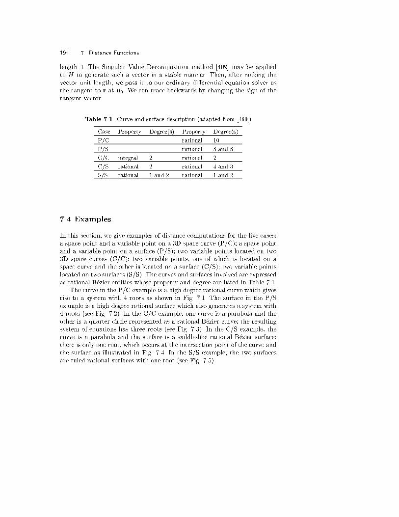
194 7. Distance Functions
length 1. The Singular Value Decomposition method [409] may be appliedto H to generate such a vector in a stable manner. Then, after making thevector unit length, we pass it to our ordinary di�erential equation solver asthe tangent to r at u0. We can trace backwards by changing the sign of thetangent vector.
Table 7.1. Curve and surface description (adapted from [460])
Case Property Degree(s) Property Degree(s)
P/C rational 10
P/S rational 8 and 8
C/C integral 2 rational 2
C/S rational 2 rational 4 and 3
S/S rational 1 and 2 rational 1 and 2
7.4 Examples
In this section, we give examples of distance computations for the �ve cases:a space point and a variable point on a 3D space curve (P/C); a space pointand a variable point on a surface (P/S); two variable points located on two3D space curves (C/C); two variable points, one of which is located on aspace curve and the other is located on a surface (C/S); two variable pointslocated on two surfaces (S/S). The curves and surfaces involved are expressedas rational B�ezier entities whose property and degree are listed in Table 7.1.
The curve in the P/C example is a high degree rational curve which givesrise to a system with 4 roots as shown in Fig. 7.1. The surface in the P/Sexample is a high degree rational surface which also generates a system with4 roots (see Fig. 7.2). In the C/C example, one curve is a parabola and theother is a quarter circle represented as a rational B�ezier curve; the resultingsystem of equations has three roots (see Fig. 7.3). In the C/S example, thecurve is a parabola and the surface is a saddle-like rational B�ezier surface;there is only one root, which occurs at the intersection point of the curve andthe surface as illustrated in Fig. 7.4. In the S/S example, the two surfacesare ruled rational surfaces with one root (see Fig. 7.5).

7.4 Examples 195
Fig. 7.1. Distances of a point and a high degree rational B�ezier curve (adaptedfrom [460])
Fig. 7.2. Distances of a point and a high order rational B�ezier surface (adaptedfrom [460])
Fig. 7.3. Distances of a rational B�ezier curve and an integral B�ezier curve (adaptedfrom [460])

196 7. Distance Functions
Fig. 7.4. Distances of a rational B�ezier curve and a rational B�ezier patch (adaptedfrom [460])
Fig. 7.5. Distances of two linear-quadratic B�ezier patches (adapted from [460])

8. Curve and Surface Interrogation
8.1 Classi�cation of interrogation methods
Interrogation is the process of extraction of information from a geometricmodel. In this chapter we focus on free-form curve and surface interrogation.Free form surfaces, also called sculptured surfaces, are widely used in scien-ti�c and engineering applications. For example, the hydrodynamic shape ofpropeller blades has an important role in marine applications, and the aerody-namic shape of turbine blades determines the performance of aircraft engines.Free-form surfaces arise also in the bodies of the ships, automobiles and air-craft, which have both functionality and attractive shape requirements. Manyelectronic devices as well as consumer products are designed with aestheticshapes, which involve free-form surfaces. During the last two decades, manycurve and surface interrogation methods have been proposed (see referencesin [274, 61]), and we will introduce some of them in this chapter.
Propeller and turbine blades are manufactured by numerically controlled(NC) milling machines. When a ball-end mill cutter is used, the cutter radiusmust be smaller than the smallest concave radius of curvature of the surface tobe machined to avoid local overcut (gouging) (see Sect. 11.1.2). Gouging is theone of the most critical problems in NC machining of free-form surfaces [184].Therefore, we must determine the distribution of the principal curvaturesof the surface, which are upper and lower bounds on the curvature at agiven point, to select the cutter size [116, 94]. Visualization techniques ofvarious curvature measures have been developed by Dill [74], Beck et al.[22], Munchmeyer [279, 278], Higashi and Kaneko [162], Pottmann and Optiz[327], Maekawa and Patrikalakis [254], Elber and Cohen [87] and Tuohy [422].Higashi et al. [163] introduced the loci of points corresponding to extrema ofcurvature values of the design surface called surface edges, which show howthe surface is waving and where the peaks of the wave exist. Kase et al. [188]presented local and global evaluation methods for shape errors of free-formsurfaces which have been applied to the evaluation of sheet metal surfaces.
Developable surfaces [13, 221, 120, 32, 325, 251, 328] are surfaces which canbe unfolded or developed onto a plane without stretching or tearing. They areof considerable importance to plate-metal-based industries as shipbuilding.For a developable surface the Gaussian curvature is zero everywhere [76].Thus the manufacturer would pro�t from prior knowledge of the distribution

198 8. Curve and Surface Interrogation
of the Gaussian curvature of the metal plate. A line of curvature indicatesa directional ow for the maximum or the minimum curvature across thesurface [22, 278, 173, 256, 250, 98] which can be used for determining feedingdirections to the rolling machine for the metal plate.
Fairing [364, 338, 144, 317, 148, 45, 316] is the process of eliminatingshape irregularities in order to produce a smoother shape. Re ection lines[201, 189, 61] are a standard surface interrogation method to assess the fair-ness of design surfaces in the automobile industry. Isophotes are used fordetection of surface irregularities [318, 144] and for continuity evaluation atthe boundaries of adjacent patches [146]. Also focal surfaces [146, 145] areused to detect undesired curvature properties of a design surface. The setof curvature extrema of a fair surface should coincide with the designer'sintention. Therefore, computation of all extrema of curvatures is desirable.The Gaussian, mean and principal curvatures are used for the detection ofsurface irregularities [279, 278, 254]. On the other hand Andersson [7] devel-oped a method to specify curvature in a surface design method and Higashiet al. [164] proposed a method to generate a smooth surface by controllingthe curvature distribution. Theisel and Farin [418] studied the curvature ofcharacteristic curves on a surface, such as contour lines, lines of curvature,asymptotic lines, isophotes and re ection lines.
As we will see in this chapter, the governing equations for shape inter-rogation often result in n polynomial equations with n unknowns when theinput curves and surfaces are in integral/rational B�ezier form. If the para-metric curves and surfaces are in integral/rational B-spline form, some shapeinterrogation methods involve a �rst step where the integral/rational B-splinecurve or surface patch is subdivided into a number of integral/rational B�eziercurves or rational B�ezier patches. In the computer implementation we evalu-ate the coe�cients of the governing nonlinear polynomial equations in multi-variate Bernstein form starting from the given input B�ezier curve or surfaceusing the arithmetic operations in Bernstein form [106, 314] (see Sect. 1.3.2).The system of nonlinear polynomial equations can be solved robustly andaccurately by the IPP algorithm presented in Chap. 4.
In this section we will classify the interrogation methods by the orderof derivatives of the curve or surface position vector which are involved. Aninterrogation method is characterized as nth-order, if derivatives of the curveor surface position vector of order n are involved.
8.1.1 Zeroth-order interrogation methods
Wireframe. The wireframe of a surface patch is produced by displayingits boundary curves and a number of other iso-parametric curves in bothparametric directions, as depicted in Fig. 8.1. Small-scale wireframes on rasterscreens provide only a rough idea of the underlying shape and are not veryappropriate means to judge the nature of the surface and its smoothness andfairness. Furthermore, depending on the density of iso-parametric lines and

8.1 Classi�cation of interrogation methods 199
their actual shape, they may mislead the designer about the actual shape ofthe surface.
Fig. 8.1. Wireframe model of bicubic B-spline patch
Contouring. A better indication of the surface is normally obtained usingcontour maps. There are di�erent types of contour maps. The simplest con-touring method is to intersect the surface with a family of user-de�ned non-uniformly spaced parallel planes [22, 95] (see Fig. 5.1). Using z = constantcontour maps, maxima, minima and saddle points of the height z(u; v) ofthe surface can be identi�ed. Contouring with planes is, for example, em-ployed in ship hull and aircraft fuselage design. More complex contouringmethods involve intersections with a series of co-axial cylinders or cones ofnon-uniformly spaced radii. Propeller and turbine blades are normally con-toured using such methods. The intersection methods of Chap. 5 need to beinvoked to perform robust contouring.
8.1.2 First-order interrogation methods
Shading and ray tracing. A shaded image of a surface usually gives a morerealistic visual representation in comparison to a wireframe model [118]. Asimple illumination model, based on Lambert's cosine law and incorporatingspecular re ection, gives the re ected intensity I as a function of the incidentintensity Ii from a point light source, the ambient intensity Ia, the di�use

200 8. Curve and Surface Interrogation
re ection constant kd, the specular re ection constant ks, the ambient di�usere ection constant ka, the angle � between the unit surface normal N anda light direction vector, and of the angle � between a viewpoint directionvector and a vector in the direction of re ection:
I = Iaka +Iir(kd cos � + ks cos�) ; (8.1)
for 0 � ka; kd; ks � 1 and 0 � � � �2 where r represents the distance from the
perspective viewpoint to the point on the surface. More complicated shadingmodels, which take into account the properties of the material, the angle ofincidence, and the wavelength of the incidence light also exist [118].
The ray tracing technique [187, 118] gives more realistic images than asimple shaded image method, but is much slower. The intensity for eachpixel is determined using a ray from the viewpoint through the pixel intothe object. Ray tracing is in fact an intersection problem. The ray to sur-face intersection is computed for every ray and surface in a scene. Usingthe ray tracing technique, the hidden surface problem is solved during suchcomputation and also other attributes, for example multiple re ections andshadowing, can be included in the model.
Isophotes. Isophotes are curves of constant light intensity on a surface, cre-ated by a point light source at in�nity with direction l (jlj = 1), speci�ed bythe user. These curves can be used for the detection of surface irregularities[318, 144]. An isophote is a curve for which the quantity
N(u; v) � l = cos � ; (8.2)
is constant and equal to c, for 0 � c � 1 and 0 � � � 90� where N(u; v)is the unit surface normal vector. When the surface is locally planar (or at) all normals are parallel and the isophotes do not generally exist. If thesurface is CM continuous then the isophote line will be CM�1 continuous. Forrendering isophotes, the values of N(u; v) � l are computed on a lattice and anumber of isophotes are generated by connecting points of equal value foundby interpolation between straddling grid points [3]. Color Plate A.1 shows
isophotes of the bicubic B-spline surface in Fig. 8.1 with l =�12 ;
12 ;
p22
�T.
Re ection lines. Re ection lines are another �rst-order interrogationmethodused in the automotive industry to assess the fairness of a surface. Re ectionlines simulate the mirror images of a number of parallel straight uorescentlights on an automobile surface. In this method, deviations of the surfacefrom a smooth shape can be detected by irregularities of the re ection lines.Originally a re ection line was de�ned as a re ected image of a linear lightsource on a surface by Klass [201]. Kaufmann and Klass [189] modi�ed theabove de�nition to reduce the computation as follows. A family of curvesqi(t), i = 1 : : : n on the surface, which are intersection curves of the surface

8.1 Classi�cation of interrogation methods 201
with a speci�c family of planes parallel to a unit vector v, are evaluated. Foreach intersection curve qi(t), parameter ti that satis�es
_qi(t)
j _qi(t)j � v = cos� ; (8.3)
is evaluated. Then points q1(t1), q2(t2); : : :, qn(tn) are connected to formthe re ection line. The procedure is repeated for di�erent values of �. If iso-parametric lines are used instead of intersection curves of the surface with afamily of parallel planes, computational e�ciency is further improved as in[3]. Choi and Lee [61] applied the Blinn-Newell type of re ection mapping[118], which uses simple and physically acceptable mapping algorithm, togenerate re ection lines on a trimmed NURBS surface. Choi and Lee [61]also provide a thorough recent review of this topic.
Color Plate A.2 depicts re ection lines on the bicubic B-spline surface
patch shown in Fig. 8.1, where values of _q(t)j _q(t)j � v with v =
�12 ;
12 ;
p22
�Tare
evaluated along iso-parametirc curves and the equal value points found byinterpolation between mesh points are connected to form the re ection lines.
Highlight lines. Beier and Chen [23] introduced the concept of a highlightline where a set of points on a surface are determined such that the distancebetween a linear light source and an extended surface normal at the highlightlines is zero (see Fig. 8.2). Let us denote the linear light source by
l(t) = a+ bt ; (8.4)
where a is a point on the linear light source, b is a directional vector and t isa parameter. Also let us de�ne the extended surface normal vector e at thesurface point q by
e(�) = q+ S� ; (8.5)
where S is the surface normal vector at q and � is a parameter. The distancebetween the two lines l(t) and e(�) is given by
d =j(b� S) � (a� q)j
jb� Sj : (8.6)
This distance d will vanish if point q is on the highlight line. If we avoid casessuch that the linear light source and the surface normal become parallel, thedenominator of (8.6) is nonzero and the governing equation for determininghighlight lines reduces to
(b� S(u; v)) � (a� q(u; v)) = 0 : (8.7)
Equation (8.7) can be traced using the same technique that we introducedin Sect. 5.8.1. Sone and Chiyokura [400] developed a method to control ahightlight line directly using a NURBS boundary Gregory patch. Zhang andCheng [459] studied a method to remove local irregularities of NURBS surfacepatches by modifying its highlight lines for real time interactive design.
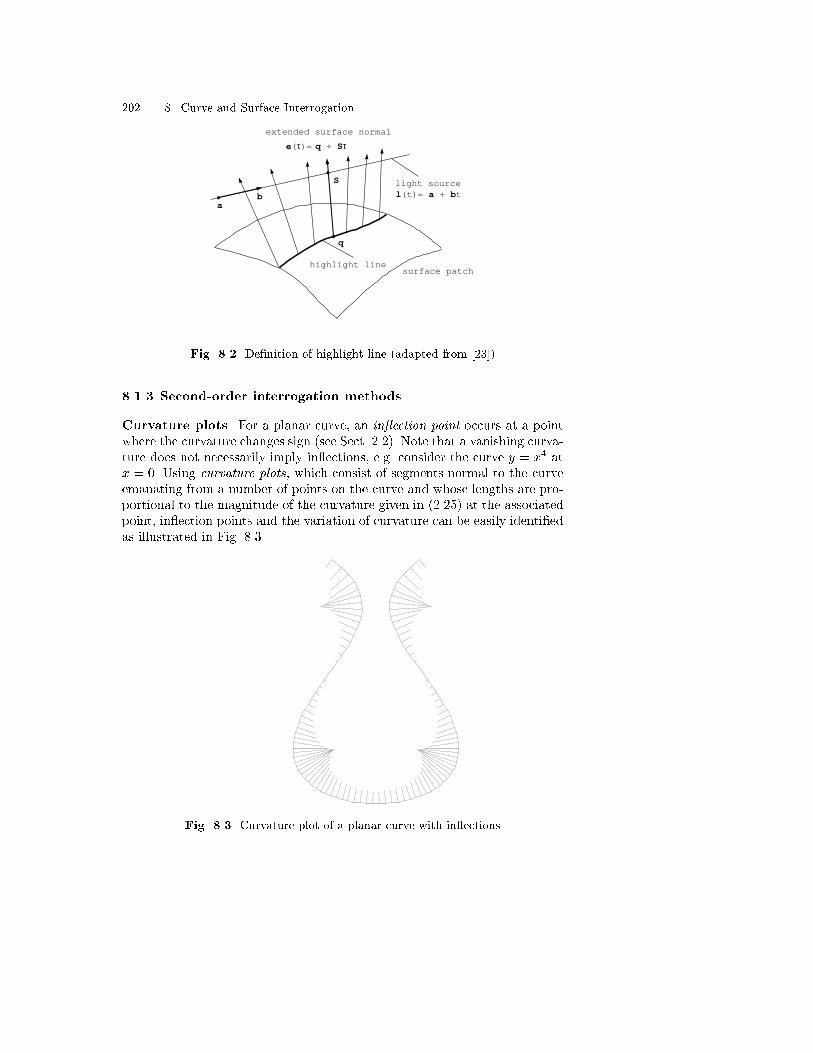
202 8. Curve and Surface Interrogation
highlight line
light source
ab
q
S
l(t)= a + bt
surface patch
extended surface normal
e(τ)= q + Sτ
Fig. 8.2. De�nition of highlight line (adapted from [23])
8.1.3 Second-order interrogation methods
Curvature plots. For a planar curve, an in ection point occurs at a pointwhere the curvature changes sign (see Sect. 2.2). Note that a vanishing curva-ture does not necessarily imply in ections, e.g. consider the curve y = x4 atx = 0. Using curvature plots, which consist of segments normal to the curveemanating from a number of points on the curve and whose lengths are pro-portional to the magnitude of the curvature given in (2.25) at the associatedpoint, in ection points and the variation of curvature can be easily identi�edas illustrated in Fig. 8.3.
Fig. 8.3. Curvature plot of a planar curve with in ections

8.1 Classi�cation of interrogation methods 203
Zero curvature points. The signed curvature formula for a planar para-metric curve is given in (2.25). Due to the regularity condition, a necessarycondition to determine in ection points is
_x(t)�y(t)� _y(t)�x(t) = 0; t 2 [t1; t2] : (8.8)
An in ection point on a planar curve is shown in Fig. 8.7, marked by �.The curvature �(t) of a space curve is given in (2.26). The formula can
be expressed as
�(t) =
p( _x�y � _y�x)2 + ( _y�z � _z�y)2 + ( _z�x� _x�z)2
( _x2 + _y2 + _z2)32
: (8.9)
Since we are assuming a regular curve, a condition to determine a point ona curve, where the curvature �(t) vanishes, is [58]
K0(t) � ( _x�y � _y�x)2 + ( _y�z � _z�y)2 + ( _z�x� _x�z)2 = 0; t 2 [t1; t2] ; (8.10)
or_x�y � _y�x = _y�z � _z�y = _z�x� _x�z = 0; t 2 [t1; t2] : (8.11)
Curvature vanishing points on a space curve r(t) are shown in Fig. 8.8, markedby �.Radial curves. For a parametric space curve r(t), a radial curve is de�nedas
f(t) = p+ n(t)=�(t) ; (8.12)
where p is a �xed reference point in space, n(t) is the unit principal normalvector and �(t) is a nonzero curvature of the curve [226]. Here the sign con-vention (a) (see Fig. 3.7 (a)) is adopted for the curvature. For sign convention(b) we simply replace the plus sign with a minus sign. Radial curves are amethod for visualizing curvature in a manner decoupled from the shape ofthe curve as illustrated in Fig. 8.4. When an in ection point is involved, asin Fig. 8.4, spikes in opposite directions occur. By viewing the radial curve,a curvature measure is visualized. However, the user is left without a directreference as to the relationship between the curve point and the curvaturevalue. The radial curve also provides a method for viewing the range of vari-ation of the curve's normal vector. This range of variation can be obtainedfrom the angular sector described by all rays emanating from p and passingthrough all points on the radial curve. Radial curves are useful in accessibilityand interference analyses.
Surface curvatures and curvature maps. Surface interrogation may beperformed using di�erent curvature measures of the surface [22, 279, 18,92]. The Gaussian, mean, absolute [92], and root mean square (rms) [245]curvatures are the product (3.61), the average (3.62), the sum of the absolutevalues

204 8. Curve and Surface Interrogation
Fig. 8.4. A radial curve of y = x3 with a �xed reference point p = (�2; 2; 0). Thethin curve is the radial curve of the thick curve (y = x3 with a curvature plot)
kabs =j kmax j + j kmin j ; (8.13)
and the square root of the sum of the squares of the principal curvatures
krms =qk2max + k2min ; (8.14)
respectively. These surface curvature functions are all scalar valued functions.The variation of any of these quantities can be displayed using a color-codedcurvature map [74, 22]. Contour lines of constant curvature can also be used todisplay and visualize the variation of these curvature functions. Munchmeyer[279] calculates the curvature on a lattice and linearly interpolates the contourpoints. Maekawa and Patrikalakis [254] present a method which allows arobust and accurate computation of all stationary points and all contour linesfor functions describing Gaussian, mean and principal curvatures of B-splinesurfaces. This method allows us to divide the surface into regions of speci�crange of curvature. A summary with further applications can be found in[254].

8.1 Classi�cation of interrogation methods 205
A surface in ection exists on a surface at a point P if the surface crossesthe tangent plane at P [172]. The point P is then called an in ection point.If the Gaussian curvature is positive at every point of a region of a surfacethen there are no in ections in that region. If the Gaussian curvature changessign in a region of a surface then there is an in ection in that region. In areaswhere the surface has Gaussian curvature very close to or equal to zero theGaussian curvature alone cannot provide adequate information about theshape of the surface. In such a case the surface has an in ection point inthe region only if the mean curvature changes sign. The Gaussian and meancurvatures together provide su�cient information in order to identify surfacein ections on a surface [278, 279].
The curvature maps of the principal curvatures can also help to select aspherical cutter of suitable radius in order to avoid gouging during machiningof the surface [22, 254]. We will discuss further on how to construct contourlines of constant curvature in Sect. 8.5.
Focal curves and surfaces. For a parametric space curve r(t), a focal curveor an evolute, shown in Fig. 8.5, is de�ned as
f(t) = r(t) + n(t)=�(t) ; (8.15)
where n(t) is a unit principal normal vector and �(t) is a nonzero curvatureof the curve. Thus the focal curve or evolute of a curve is the locus of itscenters of curvature. Focal surfaces [146, 145] can be constructed in a similarway by using the principal curvature functions of the given surface. For agiven parametric surface patch r(u; v) the two associated focal surfaces arede�ned as
f(u; v) = r(u; v) +N(u; v)=�(u; v) ; (8.16)
where N(u; v) is a unit surface normal and �(u; v) is a nonzero principalcurvature (�min(u; v) or �max(u; v)). Here sign convention (a) (see Fig. 3.7(a)) is employed for both (8.15) and (8.16). When sign convention (b) isassumed, we simply replace the plus sign by the minus sign.
Focal curves and surfaces provide another method for visualizing cur-vature. An important application of focal curves is in testing the curva-ture continuity of surfaces across a common boundary. Curves on the fo-cal surfaces of each surface, which are at the common boundary, f(t) =r(u(t); v(t)) +N(u(t); v(t))=�(u(t); v(t)), where r = r(u(t); v(t)) is the com-mon boundary curve (or linkage curve) on the progenitor surface r = r(u; v),can be compared to determine the curvature continuity of the surfaces. Ac-cording to the linkage curve theorem by Pegna and Wolter [304] two surfacesjoined with �rst-order or tangent plane continuity along a �rst-order contin-uous linkage curve can be shown to be second-order smooth on the linkagecurve if the normal curvatures along the linkage curve on each surface agreein one direction other than the tangent direction to the linkage curve. Com-parison of focal surfaces allows for a visual assessment of the accuracy for

206 8. Curve and Surface Interrogation
Fig. 8.5. Focal curve. The thin curve is the focal curve of the thick curve
the second-order contact of two patches along their linkage curve. Namelyif the two focal curve point sets (de�ned via �min and �max) of one surfacepatch agree along the linkage curve with the two corresponding focal curvepoint sets of the adjacent patch then these surface patches have curvaturecontinuous surface contact along the linkage curve. The deviation of the cor-responding focal curves indicates the amount of discontinuity of curvature ofboth adjacent patches along the linkage curve.
Orthotomics. Orthotomic curves and surfaces are used to display the anglebetween the position vector of a curve (or surface) and the normal of thecurve or surface respectively. Orthotomic curves and surfaces are useful forindicating the presence of in ection points [146]. A �-orthotomic curve y�(t)of a planar curve r(t) with respect to a point p, not on r(t) or any of itstangents, is de�ned as
y�(t) = p+ �[(r(t) � p) � n(t)]n(t) ; (8.17)
where n(t) is the unit normal vector of r(t) and � is a scaling factor chosenfor appropriate visualization. The tangent vector of an orthotomic curve iszero (and the orthotomic curve usually has a cusp-like singularity) at anyparameter value of t at which the curve r(t) has an in ection point. Anillustrative example is shown in Fig. 8.6.
A �-orthotomic surface y�(u; v) of a surface r(u; v) with respect to a pointp, not on r(u; v) or any of its tangent planes, is de�ned as
y�(u; v) = p+ �[(r(u; v) � p) �N(u; v)]N(u; v) ; (8.18)
whereN(u; v) is the unit normal vector of the surface r(u; v) and � is a scalingfactor. An orthotomic surface has a singularity, i.e. a degenerate tangentplane, at all values of u; v at which the Gaussian curvature of the surfacer(u; v) vanishes or changes sign.

8.1 Classi�cation of interrogation methods 207
Fig. 8.6. Orthotomics of two curves (adapted from [3]). Note that the orthotomicon the right shows the in ection point of the curve. The thin curves are the ortho-tomics of the thick curves
Curvature lines. A line of curvature is a curve on a surface whose tangentat every point is aligned along a principal curvature direction. We have stud-ied the basics of lines of curvature in Sect. 3.4 and will study them furtherin Chap. 9. The principal directions at a given point are those directions forwhich the normal curvature takes on minimum and maximum values. A lineof curvature indicates a directional ow for the maximum or the minimumcurvature across the surface [22]. Curvature lines provide some useful infor-mation about the surface. For example, when a plate is going to be shaped byrolling it is fed into the rolls using a principal direction and the forming rollsare adjusted according to the principal curvature [278]. The network of curva-ture lines may also be useful in idealization, meshing and structural analysisof shells with free-form surfaces as boundaries, because of their orthogonalityproperty.
Geodesics. Geodesics are curves of zero geodesic curvature on a surfaceand provide candidates for arcs of minimum length between two points ona surface [411, 234, 136]. We will study the formulation of the governingequations of geodesics on a parametric surface as well as on an implicit surfaceand their solution methodology in Chap. 10.
8.1.4 Third-order interrogation methods
Torsion of space curves. As we discussed in Sect. 2.3 torsion describesthe deviation of a space curve away from its osculating plane spanned bythe curve's tangent and normal vectors. For planar curves, the torsion isalways zero. For an arbitrary speed parametric space curve r(t), t 2 [t1; t2]the torsion at points with nonzero curvature is given by (2.48).

208 8. Curve and Surface Interrogation
From (2.48), a condition for zero torsion at a nonzero curvature point is
T0(t) � ���x ( _y�z � �y _z)+
���y ( _z�x� �z _x)+
���z ( _x�y � �x _y) = 0; t 2 [t1; t2] : (8.19)
Figure 8.8 shows a point of zero torsion, marked by � at the midpoint of thecurve. The sign of torsion has geometric signi�cance [205]. If �(t) changes itssign from +(�) to �(+) when passing a point its features change from a right-handed (left-handed) curve to a left-handed (right-handed) one, respectively.
Stationary points of curvature of planar and space curves. ModernCAD/CAM systems allow users to access speci�c application programs forperforming several tasks, such as displaying objects on a graphic display,mass property calculation, �nite element or boundary element meshing foranalysis. These application programs often operate on piecewise linear ap-proximation of the exact geometric de�nition. When a coarse approximationof good quality is required for 2-D and 3-D curves, stationary points of cur-vature play an important role in successful discretization [192, 97, 150, 58].
Using (2.25), the �rst derivative of the curvature function of a planarcurve is given by
_�(t) =( _x2 + _y2)( _x
���y � ���
x _y)� 3( _x�x+ _y�y)( _x�y � �x _y)
( _x2 + _y2)52
: (8.20)
Since we are assuming a regular curve, the necessary condition to have a localmaximum or minimum of curvature is given by
( _x2 + _y2)( _x���y � ���
x _y)� 3( _x�x+ _y�y)( _x�y � �x _y) = 0 : (8.21)
Figure 8.7 shows the corresponding stationary points of curvature on r(t),labeled by �. Furthermore, comparing (8.8) and (8.21) we see both �(t) and_�(t) of a regular planar curve r(t) vanish for some t if and only if _x�y = �x _y
and _x���y=
���x _y, simultaneously [58].
Similarly for a regular space curve, the necessary condition to have sta-tionary points of curvature �(t) at nonzero curvature points is given by
K1(t) � G1(t)G2(t)� 3G3(t)K0(t) = 0 ; (8.22)
where
G1(t) = _x2 + _y2 + _z2 ; (8.23)
G2(t) = ( _x�y � �x _y)( _x���y � ���
x _y) + ( _y�z � �y _z)( _y���z � ���
y _z) (8.24)
+( _z�x� �z _x)( _z���x � ���
z _x) ;
G3(t) = _x�x+ _y�y + _z�z ; (8.25)
and K0(t) is de�ned in (8.10). Note that at points �(t) = 0, the necessarycondition (8.22) is automatically satis�ed (see (8.11)), thus at those points_�(t) = 0 is equivalent to

8.1 Classi�cation of interrogation methods 209
Fig. 8.7. Signi�cant points on a planar B�ezier curve of degree 5 (adapted from[58])
_x���y � ���
x _y = _y���z � ���
y _z = _z���x � ���
z _x = 0 : (8.26)
Three points in Fig. 8.8 satisfy (8.22). Two of them are marked by �'s andone is marked by � at the midpoint of the curve.
Once all the stationary points are identi�ed, we may use the extrema the-ory of functions for a single variable given in Sect. 7.3.1 to classify stationarypoints of curvature.
Stationary points of curvature of parametric surfaces. Stationarypoints of surface curvature are important in methods for the correct topo-logical decomposition of the surface on the basis of curvature [254]. Letthe curvature in question of a parametric surface r = r(u; v) de�ned over(u; v) 2 [0; 1]2 be denoted by a scalar function C(u; v), then the following(see also Sect. 7.2.1), need to be evaluated to locate all the stationary pointsof curvature and to �nd the global maximum and minimum values of C(u; v)to provide a correct topological decomposition of the surface [254].
1. The four values of curvature at the parameter domain corners
C(0; 0); C(0; 1); C(1; 0); C(1; 1) : (8.27)
2. Stationary points along parameter domain boundaries (roots of the fourequations)
Cu(u; 0) = 0; Cu(u; 1) = 0; 0 � u � 1 ;
Cv(0; v) = 0; Cv(1; v) = 0; 0 � v � 1 : (8.28)

210 8. Curve and Surface Interrogation
XY
Z
X
Y
Y
Z
X
Z
Fig. 8.8. Signi�cant points on a space curve and its projections (adapted from[58])
3. Stationary points within the parameter domain (roots of the two simul-taneous equations)
Cu(u; v) = 0; Cv(u; v) = 0; 0 � u; v � 1 : (8.29)
The curvature values at the parameter domain corners are readily computed.The classi�cation of stationary points of functions of two variables is given inTheorem 7.3.1. The formulations for the stationary points of the Gaussian,mean and principal curvatures for parametric surfaces are derived in Sect.8.2.
8.1.5 Fourth-order interrogation methods
Stationary points of torsion of space curve. At nonzero curvature pointon a regular space curve where the twist out of its osculating plane attains alocal maximum or minimum, namely _�(t) = 0, leads to the necessary condi-tion [58]

8.1 Classi�cation of interrogation methods 211
T1(t) � G4(t)K0(t)� 2G2(t)T0(t) = 0; t 2 [t1; t2] ; (8.30)
where
G4(t) = x(4)( _y�z � �y _z) + y(4)( _z�x� �z _x) + z(4)( _x�y � �x _y) ; (8.31)
and K0(t), G2(t) and T0(t) are de�ned in (8.10), (8.24) and (8.19), respec-tively.
Figure 8.8 shows the corresponding signi�cant points, marked by �'s.Moreover, comparing (8.19) and (8.30), both �(t) and _�(t) of a regular curvevanish at nonzero curvature points if and only if T0(t) = G4(t) = 0.
Stationary points of total curvature. We now consider the notion of theDarboux vector (t) de�ned by [205],
(t) = �(t)t(t) + �(t)b(t) ; (8.32)
where t(t) and b(t) are the unit tangent and binormal vectors, respectively.The Darboux vector turns out to be a rotation vector of the Frenet frame whilemoving along the curve and therefore, its Euclidean norm j(t)j indicatesthe angular speed !(t) of the moving local frame. The angular speed !(t) issometimes called total curvature of a curve and de�ned by
!(t) =p�2(t) + �2(t) : (8.33)
In a planar curve, !(t) reduces to �(t) and the binormal vector becomes theaxis of rotation. We notice that the total curvature !(t) captures the couplede�ect of both intrinsic features of a space curve, and hence, we may considerit as a criterion function for detecting a signi�cant point on a space curve[58].
At a nonzero curvature point on a regular space curve, where the movingframe has its locally highest or lowest angular speed, satis�es the equation_!(t) = 0, i.e.
K30 (t)K1(t) +G4
1(t)T0(t)T1(t) = 0; t 2 [t1; t2] ; (8.34)
whereK0(t),K1(t), G1(t), T0(t) and T1(t) are de�ned in (8.10), (8.22), (8.23),(8.19) and (8.30), respectively. Comparing each function we can roughly seeeach contribution of �(t), _�(t), �(t) and _�(t) to (8.34). For a special example,if _�(t) and one of �(t) or _� (t) vanish at some t, (8.34) is also satis�ed there.We note K0(t) and G1(t) are always positive at a nonzero curvature point.Three points in Fig. 8.8 satisfy (8.34). Two points, marked by +'s, are locatedclose to the points of curvature extrema, and the other point, marked by �,is located at the midpoint of the curve where _�(t) and �(t) also vanish.
Finally, for the special case where �(t), �(t) and consequently !(t) areconstant, the curve is a circular helix.
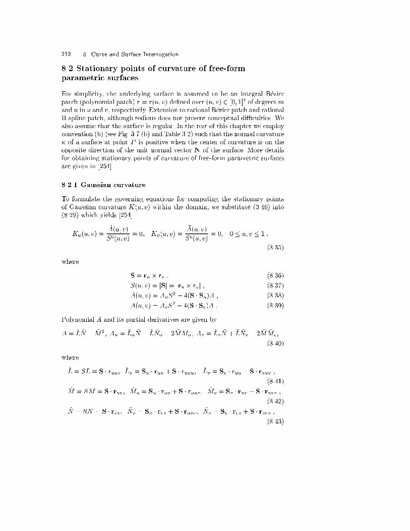
212 8. Curve and Surface Interrogation
8.2 Stationary points of curvature of free-formparametric surfaces
For simplicity, the underlying surface is assumed to be an integral B�ezierpatch (polynomial patch) r = r(u; v) de�ned over (u; v) 2 [0; 1]2 of degreesmand n in u and v, respectively. Extension to rational B�ezier patch and rationalB-spline patch, although tedious does not present conceptual di�culties. Wealso assume that the surface is regular. In the rest of this chapter we employconvention (b) (see Fig. 3.7 (b) and Table 3.2) such that the normal curvature� of a surface at point P is positive when the center of curvature is on theopposite direction of the unit normal vector N of the surface. More detailsfor obtaining stationary points of curvature of free-form parametric surfacesare given in [254].
8.2.1 Gaussian curvature
To formulate the governing equations for computing the stationary pointsof Gaussian curvature K(u; v) within the domain, we substitute (3.46) into(8.29) which yields [254]
Ku(u; v) =�A(u; v)
S6(u; v)= 0; Kv(u; v) =
�A(u; v)
S6(u; v)= 0; 0 � u; v � 1 ;
(8.35)
where
S = ru � rv ; (8.36)
S(u; v) = jSj = jru � rv j ; (8.37)�A(u; v) = AuS
2 � 4(S � Su)A ; (8.38)
�A(u; v) = AvS2 � 4(S � Sv)A : (8.39)
Polynomial A and its partial derivatives are given by
A = ~L ~N � ~M2; Au = ~Lu ~N + ~L ~Nu � 2 ~M ~Mu; Av = ~Lv ~N + ~L ~Nv � 2 ~M ~Mv;
(8.40)
where
~L = SL = S � ruu; ~Lu = Su � ruu + S � ruuu; ~Lv = Sv � ruu + S � ruuv ;(8.41)
~M = SM = S � ruv ; ~Mu = Su � ruv + S � ruuv ; ~Mv = Sv � ruv + S � ruvv ;(8.42)
~N = SN = S � rvv ; ~Nu = Su � rvv + S � ruvv ; ~Nv = Sv � rvv + S � rvvv ;(8.43)

8.2 Stationary points of curvature of free-form parametric surfaces 213
and
Su = ruu � rv + ru � ruv ; Sv = ruv � rv + ru � rvv : (8.44)
As S 6= 0, (8.35) are satis�ed if
�A(u; v) = 0; �A(u; v) = 0; 0 � u; v � 1 ; (8.45)
which are two simultaneous bivariate polynomial equations of degree (10m�7; 10n� 6), (10m� 6; 10n� 7) in u and v, respectively. For example, if theinput surface is a bicubic B�ezier patch, the degrees of the two simultaneousbivariate polynomial equations become (23, 24) and (24, 23) in u and v.System (8.45) can be solved robustly with the IPP algorithm described inChap. 4 (see [254] for details).
The stationary points along the four boundary edges are easily obtainedby solving the four univariate polynomial equations,
�A(u; 0) = 0; �A(u; 1) = 0; 0 � u � 1 ; (8.46)�A(0; v) = 0; �A(1; v) = 0; 0 � v � 1 ; (8.47)
using the IPP algorithm described in Chap. 4 (see [254] for details).
Example 8.2.1. A hyperbolic paraboloid r(u; v) = (u; v; uv)T , (u; v) 2 [0; 1]2
(bilinear surface), illustrated in Fig. 3.4, can be expressed in a B�ezier formas
r =
1Xi=0
1Xj=0
bijBi;1(u)Bj;1(v) ;
where b00 = (0; 0; 0)T , b01 = (0; 1; 0)T , b10 = (1; 0; 0)T and b11 = (1; 1; 1)T .The �rst and second fundamental form coe�cients are readily computed using(3.63) (3.64) (3.65)
E = ru � ru = 1 + v2; F = ru � rv = uv; G = rv � rv = 1 + u2 ;
N =(�v;�u; 1)Tpu2 + v2 + 1
;
L = ruu �N = 0; M = ruv �N =1p
u2 + v2 + 1; N = rvv �N = 0 :
Thus the Gaussian curvature is given by
K =LN �M2
EG� F 2= � 1
u2 + v2 + 1:
The Gaussian curvature is always negative and hence all the points are hy-perbolic.

214 8. Curve and Surface Interrogation
The stationary points within the parameter domain are given by �ndingthe roots of Ku = Kv = 0. Since
S = ru � rv = (�v;�u; 1)T ; S = jSj =pu2 + v2 + 1 ;
Su = (0;�1; 0)T ; Sv = (�1; 0; 0)T ;
and from (8.40) through (8.43)
~L = SL = 0; ~M = SM = 1; ~N = SN = 0 ;
A = ~L ~N � ~M2 = �1 ;Au = ~Lu ~N + ~L ~Nu � 2 ~M ~Mu = 0; Av = ~Lv ~N + ~L ~Nv � 2 ~M ~Mv = 0 ;
and from (8.38) and (8.39)
�A = AuS2 � 4(S � Su)A = 4u; �A = AvS
2 � 4(S � Sv)A = 4v ;
hence we have
Ku =4u
(u2 + v2 + 1)3; Kv =
4v
(u2 + v2 + 1)3:
Thus the stationary point within the domain is given by (u; v) = (0; 0), whichcoincides with one of the corner points of the bilinear surface patch. UsingTheorem 7.3.1, we �nd that K(0; 0) = �1 is a minimum.
At the remaining of corner points of the patch, we can readily compute
K(0; 1) = �14; K(1; 0) = �1
4; K(1; 1) = �1
9:
Stationary points along parameter domain boundaries are obtained by solvingthe following four univariate equations
Ku(u; 0) =4u
(u2 + 1)3= 0 ;
Ku(u; 1) =4u
(u2 + 2)3= 0 ;
Kv(0; v) =4v
(v2 + 1)3= 0 ;
Kv(1; v) =4v
(v2 + 2)3= 0 :
The roots are u = 0, u = 0, v = 0 and v = 0, thus they coincide withthe corner points (0; 0), (0; 1), (0; 0) and (1; 0). Therefore, the range of theGaussian curvature is �1 � K � � 1
9 .

8.2 Stationary points of curvature of free-form parametric surfaces 215
8.2.2 Mean curvature
Similarly to the Gaussian curvature, we have the following equations to eval-uate the stationary points of mean curvature H given by (3:47) (convention(b) (see Fig. 3.7 (b) and Table 3.2) is employed) within the domain [254]:
Hu(u; v) =�B(u; v)
2S5(u; v)= 0; Hv(u; v) =
�B(u; v)
2S5(u; v)= 0; 0 � u; v � 1 ;
(8.48)
where
�B(u; v) = BuS2 � 3(S � Su)B ; (8.49)
�B(u; v) = BvS2 � 3(S � Sv)B : (8.50)
Polynomial B and its partial derivatives are given by
B = 2F ~M �E ~N �G~L ; (8.51)
Bu = 2(F ~Mu + Fu ~M) � (Eu ~N +E ~Nu) � (Gu~L+G~Lu) ; (8.52)
Bv = 2(F ~Mv + Fv ~M) � (Ev ~N +E ~Nv) � (Gv~L+G~Lv) ; (8.53)
where
Eu = 2ru � ruu; Ev = 2ru � ruv ; (8.54)
Fu = ruu � rv + ru � ruv ; Fv = ruv � rv + ru � rvv ; (8.55)
Gu = 2rv � ruv ; Gv = 2rv � rvv : (8.56)
Since S 6= 0, (8.48) reduce to two simultaneous bivariate polynomial equa-tions
�B(u; v) = 0; �B(u; v) = 0; 0 � u; v � 1 ; (8.57)
of degree (9m � 6; 9n � 5) and (9m � 5; 9n � 6) in u and v. For a bicubicB�ezier patch input, the degrees of the governing equations are (21, 22) and(22, 21) in u and v, respectively. The system (8.57) can be solved robustlywith the IPP algorithm described in Chap. 4 (see [254] for details).
The stationary points of mean curvature along the domain boundary canbe obtained by solving the following four univariate polynomial equations:
�B(u; 0) = 0; �B(u; 1) = 0 ; 0 � u � 1 ; (8.58)�B(0; v) = 0; �B(1; v) = 0 : 0 � v � 1 : (8.59)
These equations can be solved robustly with the IPP algorithm described inChap. 4 (see [254] for details).

216 8. Curve and Surface Interrogation
8.2.3 Principal curvatures
For obtaining the stationary points of principal curvature � within the do-main, the simultaneous bivariate equations (8.29) become [254]
�u(u; v) =f1(u; v)� f2(u; v)
pf3(u; v)
2S5(u; v)pf3(u; v)
= 0; 0 � u; v � 1 ; (8.60)
�v(u; v) =g1(u; v)� g2(u; v)
pf3(u; v)
2S5(u; v)pf3(u; v)
= 0; 0 � u; v � 1 :
The plus and minus signs correspond to the maximum and minimum principalcurvatures, and f1(u; v), f2(u; v), f3(u; v), g1(u; v) and g2(u; v) are polyno-mials of degree (14m � 9; 14n � 8), (9m � 6; 9n � 5), (10m � 6; 10n � 6),(14m� 8; 14n� 9), (9m� 5; 9n� 6) in u and v parameters and are given by
f1(u; v) = (BBu � 2AuS2)S2 + (8AS2 � 3B2)(S � Su) ; (8.61)
f2(u; v) = BuS2 � 3(S � Su)B ; (8.62)
f3(u; v) = B2 � 4AS2 ; (8.63)
g1(u; v) = (BBv � 2AvS2)S2 + (8AS2 � 3B2)(S � Sv) ; (8.64)
g2(u; v) = BvS2 � 3(S � Sv)B : (8.65)
Assuming f3 6= 0 and S 6= 0, we obtain
f1(u; v) � f2(u; v)pf3(u; v) = 0; 0 � u; v � 1 ; (8.66)
g1(u; v) � g2(u; v)pf3(u; v) = 0; 0 � u; v � 1 :
These are two simultaneous bivariate irrational equations involving polyno-mials and square roots of polynomials which arise from the analytical expres-sions of principal curvatures. We can introduce an auxiliary variable � suchthat �2 = f3 to remove the radical and transform the problem into a sys-tem of three trivariate polynomial equations of degree (14m� 9; 14n� 8; 1),(14m � 8; 14n � 9; 1), (10m � 6; 10n � 6; 2) in u, v and � . For a bicubicB�ezier patch the degrees of the trivariate polynomial equations are (33,34,1),(34,33,1) and (24,24,2). The resulting system can be solved with the IPPalgorithm of Chap. 4 (see [254] for details).
For the stationary points of principal curvatures along the boundary, weneed to solve the following four univariate irrational equations involving poly-nomials and square roots of polynomials
f1(u; 0) � f2(u; 0)pf3(u; 0) = 0; f1(u; 1)� f2(u; 1)
pf3(u; 1) = 0; 0 � u � 1 ;
(8.67)
g1(0; v) � g2(0; v)pf3(0; v) = 0; g1(1; v)� g2(1; v)
pf3(1; v) = 0; 0 � v � 1 ;
(8.68)
which can be solved by the same auxiliary variable method as before.

8.3 Stationary points of curvature of explicit surfaces 217
When f3 = 0 (or equivalently H2 � K = 0 if S 6= 0), (8.60) becomesingular. This condition is equivalent to the point where the two principalcurvatures are identical, i.e. an umbilical point. If the umbilical point coin-cides with a local maximum or minimum of the curvature, we cannot use(8.66) to locate such a point. In such case we need to locate the umbilicalpoint �rst by �nding the roots of the equation
H2(u; v)�K(u; v) =f3(u; v)
4S6(u; v)= 0 ; (8.69)
which reduces to solving f3(u; v) = 0, since S 6= 0. BecauseW (u; v) � f3(u;v)4S6(u;v)
is a non-negative function,W (u; v) has a global minimum at the umbilic [256].The condition for global minimum at the umbilic implies that rW = 0 orequivalently (given that f3(u; v) = 0)
Wu =@f3@u
4S6= 0; Wv =
@f3@v
4S6= 0 : (8.70)
Therefore, assuming S 6= 0, the umbilics are the solutions of the followingthree simultaneous equations (see also Sect. 9.3):
@f3(u; v)
@u= 0;
@f3(u; v)
@v= 0; f3(u; v) = 0; 0 � u; v � 1 : (8.71)
These equations can be reduced to [256]:
BBu � 2AuS2 � 4A(S � Su) = 0; BBv � 2AvS
2 � 4A(S � Sv) = 0 ;
B2 � 4AS2 = 0; 0 � u; v � 1 : (8.72)
Since f3(u; v) = 0 at the umbilics, (8.66) reduce to f1(u; v) = 0 , g1(u; v) = 0.If we substitute the �rst equation of (8.72) into (8.61) and use the factf3 = B2 � 4AS2 = 0, we obtain f1(u; v) = 0. Similarly by substituting thesecond equation of (8.72) into (8.64), we obtain g1(u; v) = 0. Consequentlythe solutions of (8.66) include not only the locations of extrema of principalcurvatures but also the locations of the umbilical points. Then we use The-orem 9.5.1 at the umbilical points to check if the umbilical point is a localextremum of principal curvatures.
A cusp is an isolated singular point on the surface where the surface tan-gent plane is unde�ned, i.e. ru�rv = 0. Cusps of an o�set surface correspondto points on the progenitor where both of the principal curvatures are equalto � 1
d where d is the o�set distance [94] (see also Sect. 11.3.2). In this man-ner, cusps on an o�set surface are associated with umbilics of the progenitor.Hence we can locate the cusps on an o�set surface using (8.71).
8.3 Stationary points of curvature of explicit surfaces
We can apply the procedures discussed in Sect. 8.2 to obtain the stationarypoints of curvature of explicit surfaces [247]. Locally any surface can be ex-

218 8. Curve and Surface Interrogation
pressed as a graph of a di�erentiable function [76]. Given a point P on theparametric surface S, we can set an orthogonal Cartesian coordinate systemxyz such that xy-plane coincides with the tangent plane of S at P and z-axis is along the normal at P . It follows that in the neighborhood of P anyparametric surface S can be represented in the form r(x; y) = [x; y; h(x; y)]T ,where h is a di�erentiable function with h(0; 0) = hx(0; 0) = hy(0; 0) = 0.
We can Taylor expand h(x; y) about (0; 0) as follows
h(x; y) = h(0; 0) + [xhx(0; 0) + yhy(0; 0)] (8.73)
+1
2![x2hxx(0; 0) + 2xyhxy(0; 0) + y2hyy(0; 0)]
+1
3![x3hxxx(0; 0) + 3x2yhxxy(0; 0) + 3xy2hxyy(0; 0) + y3hyyy(0; 0)]
+R(x; y)(jx; yj3) ;where R(x; y) is a remainder term with limx!0;y!0R(x; y) = 0 and jx; yj =px2 + y2. If we take into account that h(0; 0) = hx(0; 0) = hy(0; 0) = 0, we
can consider
h(x; y) =1
2[hxx(0; 0)x
2 + 2hxy(0; 0)xy + hyy(0; 0)y2] ; (8.74)
as the second order approximation of h(x; y).If we denote E, F , G and L, M , N as coe�cients of the �rst and second
fundamental forms of the surface, and assume further that x and y axes are di-rected along the principal directions at P , assuming P is not an umbilic, then
F =M = 0 [76]. It follows that hxy(0; 0) = 0, since M = hxy=q1 + h2x + h2y
(see Equation (3.65)). Although we have assumed P is not an umbilic, we canshow that hxy(0; 0) will also vanish when the point is an umbilic (see Sect.9.2). Also the principal curvatures at P when F = M = 0 can be expressedas follows:
� If hxx(0; 0) > hyy(0; 0); (8.75)
�min = �LE
= �hxx(0; 0); �max = �NG
= �hyy(0; 0) ;� If hxx(0; 0) < hyy(0; 0); (8.76)
�max = �LE
= �hxx(0; 0); �min = �NG
= �hyy(0; 0) ;
where the minus signs are due to convention (b) of the normal curvature (seeFig. 3.7 (b)).
If we set � = hxx(0; 0) and � = hyy(0; 0) and assuming that P is a nonpla-nar point, the surface can be written locally as a second order approximationin the nonparametric form given by
z =1
2(�x2 + �y2) : (8.77)

8.3 Stationary points of curvature of explicit surfaces 219
Its corresponding parametric form is
r(x; y) = [x; y;1
2(�x2 + �y2)]T : (8.78)
Equation (8.77) or (8.78) represents an explicit quadratic surfaces which canbe categorized into four types according to combinations of � and � as listedin Table 8.1. The four types of explicit quadratic surfaces are depicted in Fig.8.9.
Table 8.1. Four types of explicit quadratic surfaces according to � and � (adaptedfrom [247])
Signs of � and � Types of surfaces Types of points at P
�� < 0 Hyperbolic paraboloid Hyperbolic point
�� > 0 and � 6= � Elliptic paraboloid Elliptic point
� = � Paraboloid of revolution Umbilical point� = 0 or � = 0 Parabolic cylinder Parabolic point
Since any regular surface can be locally approximated in the neighbor-hood of a point P by an explicit quadratic surface to the second order, weexamine the stationary points of curvatures of explicit quadratic surfaces asrepresentatives of explicit surfaces. We can apply the procedures in Sect. 8.2to evaluate the stationary points of curvatures of explicit quadratic surfaces.We will only examine the stationary points of principal curvatures, sincethose of Gaussian and mean curvatures can be found in a similar way. In thesequel we assume that � > 0 and � � � without loss of generality. It followsthat at (0,0,0) (8.76) holds and the x-axis will be the direction of maximumprincipal curvature and y-axis will be the direction for the minimum princi-pal curvature. The surface is a hyperbolic paraboloid when � < 0, an ellipticparaboloid when 0 < � < �, a paraboloid of revolution when 0 < � = �, anda parabolic cylinder when � = 0. The paraboloid and the parabolic cylindercan be considered as degenerate cases of the elliptic paraboloid.
Gaussian curvature (see (3.66)) and mean curvature (see (3.67) in Table3.2) are readily evaluated
K(x; y) =��
(1 + �2x2 + �2y2)2; H(x; y) = ��+ � + ��(�x2 + �y2)
2(1 + �2x2 + �2y2)32
;
(8.79)
and hence the principal curvatures become
�max(x; y) =�(1 + �2x2)� � (1 + �2y2)�
2(1 + �2x2 + �2y2)32
(8.80)

220 8. Curve and Surface Interrogation
(a) (b)
(c) (d)
Fig. 8.9. Explicit quadratic surfaces z = 12(�x2 + �y2) (adapted from [247]): (a)
hyperbolic paraboloid (� = �3, � = 1), (b) elliptic paraboloid (� = 1, � = 3), (c)paraboloid of revolution(� = � = 3), (d) parabolic cylinder (� = 0, � = 3)
+
p(�� �)2 � 2��(�� �)(�x2 � �y2) + �2�2(�x2 + �y2)2
2(1 + �2x2 + �2y2)32
;
�min(x; y) =�(1 + �2x2)� � (1 + �2y2)�
2(1 + �2x2 + �2y2)32
(8.81)
�p(�� �)2 � 2��(�� �)(�x2 � �y2) + �2�2(�x2 + �y2)2
2(1 + �2x2 + �2y2)32
:
The stationary points of principal curvature in the domain must satisfythe simultaneous equations (8.66). The equations not only �nd the stationarypoints of principal curvatures but also �nd the locations of the umbilics (seeSect. 8.2.3 and [254]). For explicit quadratic surface f1, f2, f3, g1, g2 (see
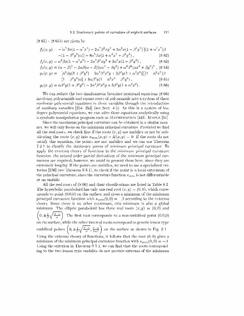
8.3 Stationary points of curvature of explicit surfaces 221
(8.61) - (8.65)) are given by
f1(x; y) = �[�2�x(1 + �2x2)� 2�2�3xy2 + 3�3x(1 + �2y2)][(1 + �2x2)�
+(1 + �2y2)�)] + 8�3�x(1 + �2x2 + �2y2) ; (8.82)
f2(x; y) = �2�x(1 + �2x2)� 2�2�3xy2 + 3�3x(1 + �2y2) ; (8.83)
f3(x; y) = (�� �)2 � 2��(�� �)(�x2 � �y2) + �2�2(�x2 + �y2)2 ; (8.84)
g1(x; y) = �[�2�y(1 + �2y2)� 2�3�2x2y + 3�3y(1 + �2x2)][(1 + �2x2)�
+(1 + �2y2)�] + 8��3y(1 + �2x2 + �2y2) ; (8.85)
g2(x; y) = ��2y(1 + �2y2)� 2�3�2x2y + 3�3y(1 + �2x2) : (8.86)
We can reduce the two simultaneous bivariate irrational equations (8.66)involving polynomials and square roots of polynomials into a system of threenonlinear polynomial equations in three variables through the introductionof auxiliary variables [254, 253] (see Sect. 4.5). As this is a system of lowdegree polynomial equations, we can solve these equations analytically usinga symbolic manipulation program such asMathematica [445], Maple [51].
Since the maximum principal curvature can be obtained in a similar man-ner, we will only focus on the minimum principal curvature. Provided we �ndall the real roots, we check �rst if the roots (x; y) are umbilics or not by sub-stituting the roots (x; y) into �min(x; y) � H(x; y) = 0. If the roots do notsatisfy this equation, the points are not umbilics and we can use Theorem7.3.1 to classify the stationary points of minimum principal curvature. Toapply the extrema theory of functions to the minimum principal curvaturefunction, the second order partial derivatives of the minimum principal cur-vatures are required; however, we avoid to present these here, since they areextremely lengthy. If the points are umbilics, we need to use a specialized cri-terion [256] (see Theorem 9.5.1), to check if the point is a local extremum ofthe principal curvature, since the curvature function �min is not di�erentiableat an umbilic.
All the real roots of (8.66) and their classi�cations are listed in Table 8.2.The hyperbolic paraboloid has only one real root (x; y) = (0; 0), which corre-sponds to point (0,0,0) on the surface, and gives a minimum of the minimumprincipal curvature function with �min(0; 0) = �� according to the extrematheory. Since there is no other extremum, this minimum is also a globalminimum. The elliptic paraboloid has three real roots (x; y) = (0; 0) and�0;� 1
�
q����
�. The �rst root corresponds to a non-umbilical point (0,0,0)
on the surface, while the other two real roots correspond to generic lemon type
umbilical points
�0;� 1
�
q���� ; ���2��
�on the surface as shown in Fig. 9.1.
Using the extrema theory of functions, it follows that the root (0; 0) gives aminimum of the minimum principal curvature function with �min(0; 0) = ��.Using the criterion in Theorem 9.5.1, we can �nd that the roots correspond-ing to the two lemon type umbilics do not provide extrema of the minimum

222 8. Curve and Surface Interrogation
Table 8.2. Classi�cation of roots according to types of explicit quadratic surfaces
Types of surfaces Hyperbolic Elliptic paraboloidparaboloid
Signs of � and � � < 0 < � 0 < � < �# of real roots 1 3
Roots (0,0) (0,0)
�0;� 1
�
q����
�Classi�cation Minimum Minimum Lemon type umbilics�min(x; y) at roots �� �� ��p�
�
Types of surfaces Paraboloid Parabolic cylinderof revolution
Signs of � and � 0 < � = � 0 = � < �# of real roots 1 1Roots (0,0) Along x-axisClassi�cation Minimum Minima�min(x; y) at roots �� ��
principal curvature function. Consequently the minimum �� is a global min-imum.
As � approaches �, two generic umbilics merge to one non-generic um-bilic at (0; 0; 0), and the surface reduces to a paraboloid of revolution asillustrated in Fig. 9.1. The paraboloid of revolution has only one real root(x; y) = (0; 0), which corresponds to point (0,0,0) on the surface, and is anon-generic umbilical point as mentioned above. Since the root correspondsto an umbilical point, we cannot use the extrema theory of functions, nor canwe use the criterion in Theorem 9.5.1, since all the second derivatives of W(see (9.25)) vanish. But it is apparent that the paraboloid of revolution has aglobal minimum of the minimum principal curvature function at the umbilicwith �min(0; 0) = ��, since the paraboloid of revolution can be constructedby rotating a parabola, which has a global minimum of its curvature at theorigin, around the z-axis. Here we are employing the sign convention (b) (seeFig. 3.7 (b) and Table 3.2) of the curvature.
In the case of a parabolic cylinder, the minimum principal curvature re-duces to a simple univariate function
�min(y) = ��(1 + �2y2)�32 : (8.87)
It is easy to show that (8.87) has a global minimum at y = 0. Therefore theparabolic cylinder has global minima with value �min = �� along the x-axis.These discussions lead to the following lemma [247]:
Lemma 8.3.1. The minimum principal curvature function of explicit quadraticsurfaces, except for the parabolic cylinder, has only one extremum at (0; 0)with value ��, which corresponds to the point (0; 0; 0) on the surface, and itis a global minimum. The parabolic cylinder has global minima �� at y = 0,which corresponds to the x-axis on the surface, and has no other extrema.

8.4 Stationary points of curvature of implicit surfaces 223
Similarly we can deduce the following lemma [247].
Lemma 8.3.2. The maximum principal curvature function of explicit quadraticsurfaces, except for the parabolic cylinder has only one extremum at (0; 0)with value ��, which corresponds to the point (0; 0; 0) on the surface, andit is a global minimum for elliptic paraboloid and paraboloid of revolution,while it is a global maximum for hyperbolic paraboloid (note that for hyper-bolic paraboloid � is negative). The maximum principal curvature function ofparabolic cylinders is zero everywhere.
Note that Lemmata 8.3.1 and 8.3.2 are based on convention (b) of the normalcurvature (see Fig. 3.7 (b)), and will be used in Sect. 11.3.4.
8.4 Stationary points of curvature of implicit surfaces
Now we provide a method to evaluate the stationary points of a curvaturefunction C(x; y; z) of implicit surfaces
f(x; y; z) = 0 : (8.88)
We want to maximize or minimize the function C(x; y; z) subject to a con-straint (8.88). Introducing the Lagrange multiplier � and the auxiliary func-tion [166]
�(x; y; z) = C(x; y; z) + �f(x; y; z) ; (8.89)
the necessary conditions for the auxiliary function �(x; y; z) to attain a localmaximum or minimum, when no constraints are imposed, are
�x = 0; �y = 0; �z = 0 : (8.90)
Equations (8.90) together with (8.88) form four equations with four unknownsx, y, z and �. The curvature functions C(x; y; z) including Gaussian, meanand principal curvatures are evaluated using the procedure described in Sect.3.5.2. In a manner similar to parametric surfaces, the denominator and thenumerator of the curvature functions consist of polynomials and square rootof polynomials if f(x; y; z) is a polynomial.
As an illustrative example, we will examine the stationary points of theminimum principal curvature �min(x; y; z) of an ellipsoid (3.83) [248] wherewe assume a � b � c. The auxiliary function becomes
� = �min(x; y; z) + �
�x2
a2+y2
b2+z2
c2� 1
�; (8.91)
and hence the system of equations to obtain the stationary points of minimumprincipal curvature of an ellipsoid reduce to

224 8. Curve and Surface Interrogation
�x(x; y; z) = �x(x; y; z) +2x�
a2= 0 ; (8.92)
�y(x; y; z) = �y(x; y; z) +2y�
b2= 0 ; (8.93)
�z(x; y; z) = �z(x; y; z) +2z�
c2= 0 ; (8.94)
x2
a2+y2
b2+z2
c2� 1 = 0 ; (8.95)
where for simplicity we have set � = �min.After some algebraic manipulation, we obtain
x(g1 + g2t+ 4�a4b2c2f22�t) = 0 ; (8.96)
y(h1 + h2t+ 4�a2b4c2f22�t) = 0 ; (8.97)
z(p1 + p2t+ 4�a2b2c4f22�t) = 0 ; (8.98)
x2
a2+y2
b2+z2
c2� 1 = 0 ; (8.99)
t2 � g3 = 0 ; (8.100)
�2 � f2 = 0 ; (8.101)
where the last two equations are added through the introduction of auxiliaryvariables t and � to remove the square roots of polynomials that appear inthe denominator and numerator of the expression in (3.83), and
f1 = x2 + y2 + z2 � a2 � b2 � c2 ; (8.102)
f2 =x2
a4+y2
b4+z2
c4; (8.103)
g1 = �2f1f2a4 � 8a2b2c2f2 + 3f21 ; (8.104)
g2 = 2a4f2 � 3f1 ; (8.105)
g3 = f21 � 4a2b2c2f2 ; (8.106)
h1 = �2f1f2b4 � 8a2b2c2f2 + 3f21 ; (8.107)
h2 = 2b4f2 � 3f1 ; (8.108)
p1 = �2f1f2c4 � 8a2b2c2f2 + 3f21 ; (8.109)
p2 = 2c4f2 � 3f1 : (8.110)
Now the system consists of six equations with six unknowns x, y, z, �, tand �. Since the degree of the polynomials is low we can solve the systemby a symbolic manipulation program such as Mathematica [445], Maple
[51], which gives a global minimum of �min equal to ac2 at (�a; 0; 0), a local
minimum bc2 at (0;�b; 0) and a global maximum c
b2 at (0; 0;�c).
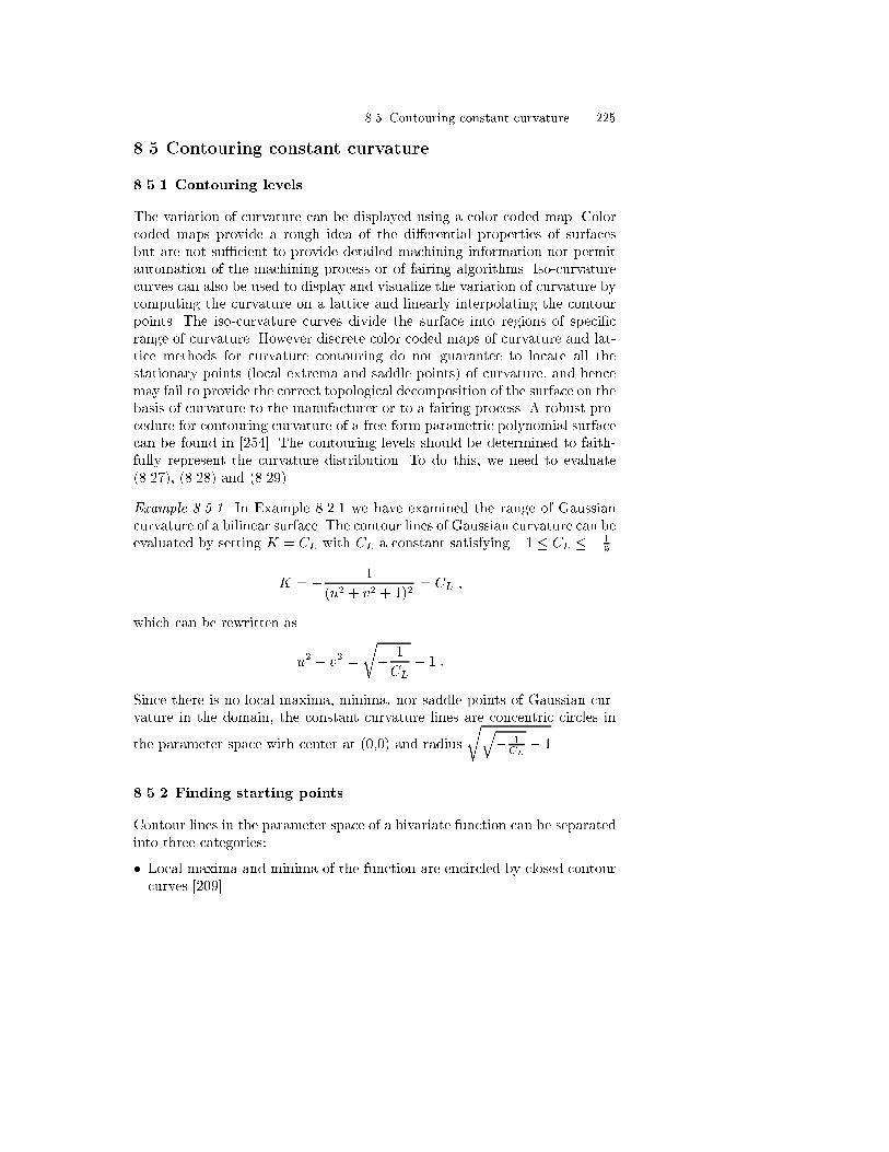
8.5 Contouring constant curvature 225
8.5 Contouring constant curvature
8.5.1 Contouring levels
The variation of curvature can be displayed using a color coded map. Colorcoded maps provide a rough idea of the di�erential properties of surfacesbut are not su�cient to provide detailed machining information nor permitautomation of the machining process or of fairing algorithms. Iso-curvaturecurves can also be used to display and visualize the variation of curvature bycomputing the curvature on a lattice and linearly interpolating the contourpoints. The iso-curvature curves divide the surface into regions of speci�crange of curvature. However discrete color coded maps of curvature and lat-tice methods for curvature contouring do not guarantee to locate all thestationary points (local extrema and saddle points) of curvature, and hencemay fail to provide the correct topological decomposition of the surface on thebasis of curvature to the manufacturer or to a fairing process. A robust pro-cedure for contouring curvature of a free-form parametric polynomial surfacecan be found in [254]. The contouring levels should be determined to faith-fully represent the curvature distribution. To do this, we need to evaluate(8.27), (8.28) and (8.29).
Example 8.5.1. In Example 8.2.1 we have examined the range of Gaussiancurvature of a bilinear surface. The contour lines of Gaussian curvature can beevaluated by setting K = CL with CL a constant satisfying �1 � CL � � 1
9
K = � 1
(u2 + v2 + 1)2= CL ;
which can be rewritten as
u2 + v2 =
r� 1
CL� 1 :
Since there is no local maxima, minima, nor saddle points of Gaussian cur-vature in the domain, the constant curvature lines are concentric circles in
the parameter space with center at (0,0) and radius
rq� 1CL� 1.
8.5.2 Finding starting points
Contour lines in the parameter space of a bivariate function can be separatedinto three categories:
� Local maxima and minima of the function are encircled by closed contourcurves [209].

226 8. Curve and Surface Interrogation
� At the precise level of a saddle point, the contour curves cross (self-intersect) or exhibit more complex behavior (eg. z = constant contourlines of monkey saddle z = x3 � 3xy2, dog saddle z = 4x3y � 4xy3 etc,[204]).
� Contour curves start from a domain boundary point and end at a domainboundary point.
If the surface is subdivided along the iso-parametric lines which contain thelocal maxima and minima of curvature inside the domain and the contour-ing levels of curvature are chosen such that the contour curves avoid saddlepoints, as shown in Figs. A.3, A.4, A.5, A.6, each sub-patch will contain sim-ple contour branches without loops or singularities. Therefore we can �nd allthe starting points of the various levels of contour curves along the parame-ter domain boundary of each sub-patch by �nding the roots of the followingequations.
Starting with the Gaussian curvature
K(u; 0) =A(u; 0)
S4(u; 0)= CK ; K(u; 1) =
A(u; 1)
S4(u; 1)= CK ; 0 � u � 1 ; (8.111)
K(0; v) =A(0; v)
S4(0; v)= CK ; K(1; v) =
A(1; v)
S4(1; v)= CK ; 0 � v � 1 ; (8.112)
where CK is the constant Gaussian curvature value. These equations can berewritten as follows:
CKS4(u; 0)�A(u; 0) = 0; CKS
4(u; 1)�A(u; 1) = 0; 0 � u � 1 ; (8.113)
CKS4(0; v)�A(0; v) = 0; CKS
4(1; v)�A(1; v) = 0; 0 � v � 1 : (8.114)
Equations (8.113), (8.114) are univariate polynomials of degree 8m-4 and8n-4, respectively.
Similarly for the mean curvature
H(u; 0) =B(u; 0)
2S3(u; 0)= CH ; H(u; 1) =
B(u; 1)
2S3(u; 1)= CH ; 0 � u � 1 ; (8.115)
H(0; v) =B(0; v)
2S3(0; v)= CH ; H(1; v) =
B(1; v)
2S3(1; v)= CH ; 0 � v � 1 ; (8.116)
where CH is the constant mean curvature value. These equations can berewritten as follows
B(u; 0)� 2CHpS2(u; 0)S2(u; 0) = 0; B(u; 1)� 2CH
pS2(u; 1)S2(u; 1) = 0 ;
(8.117)
B(0; v)� 2CHpS2(0; v)S2(0; v) = 0; B(1; v)� 2CH
pS2(1; v)S2(1; v) = 0 ;
(8.118)
where 0 � u; v � 1. Equations (8.117), (8.118) are the univariate irrationalfunctions involving polynomials and square roots of polynomials which come

8.5 Contouring constant curvature 227
from the normalization of the normal vector of the surface (see (3.3)). B(u; v)is a polynomial of degree (5m � 3; 5n � 3) and S2(u; v) is a polynomial ofdegree (4m� 2; 4n� 2).
Finally for the principal curvatures
�(u; 0) =B(u; 0)�
pf3(u; 0)
2S3(u; 0)= C� ; (8.119)
�(u; 1) =B(u; 1)�
pf3(u; 1)
2S3(u; 1)= C� ; (8.120)
�(0; v) =B(0; v)�
pf3(0; v)
2S3(0; v)= C� ; (8.121)
�(1; v) =B(1; v)�
pf3(1; v)
2S3(1; v)= C� ; (8.122)
where 0 � u; v � 1, the � signs correspond to the maximum and minimumprincipal curvatures, and C� is the constant value of principal curvature andf3(u; v) is a polynomial function de�ned in (8.63). Equations (8.119) through(8.122) can be rewritten as follows:
B(u; 0) �pf3(u; 0)� 2C�S
2(u; 0)pS2(u; 0) = 0; 0 � u � 1 ; (8.123)
B(u; 1) �pf3(u; 1)� 2C�S
2(u; 1)pS2(u; 1) = 0; 0 � u � 1 ; (8.124)
B(0; v) �pf3(0; v)� 2C�S
2(0; v)pS2(0; v) = 0; 0 � v � 1 ; (8.125)
B(1; v) �pf3(1; v)� 2C�S
2(1; v)pS2(1; v) = 0; 0 � v � 1 : (8.126)
Equations (8.123) through (8.126) are the univariate irrational functions in-volving polynomials and two square roots of polynomials which come fromthe analytical expression of the principal curvature and normalization of thenormal vector of the surface. The starting points for contour curves of cur-vature occur in pairs, since non-loop contour lines must start from a domainboundary and must end at a domain boundary point.
Ridges are surface curves where the surface tangent plane is unde�ned, i.e.ru�rv = 0. Ridges of an o�set surface correspond to points on the progenitorwhere one of the principal curvatures is equal to � 1
d (d is the o�set distance)[94]. Therefore we can use (8.123) through (8.126) to compute the startingpoints for tracing ridges on the o�set, if the surface is subdivided along theiso-parametric lines which contain the local maxima and minima of principalcurvatures, such that each sub-patch will not contain loops nor singularitiesof ridges in its interior.
8.5.3 Mathematical formulation of contouring
Contour curves for constant curvature satisfy the following equation
C(u; v) = constant ; (8.127)

228 8. Curve and Surface Interrogation
where C(u; v) is a curvature at the given point (u; v). The procedure fortracing contour curves is same as that of tracing method in the intersectionproblem that we discussed in Sect. 5.8.1. We now consider a space curve whichlies on the surface represented by the parametric form r(t) = r[u(t); v(t)].Di�erentiating (8.127) with respect to t yields
Cu _u+ Cv _v = 0 ; (8.128)
where _u, _v are the �rst derivatives with respect to t, and ( _u, _v) gives thedirection of the contour line in parameter space. The solutions to (8.128) canbe written as
_u = �Cv ; _v = ��Cu ; (8.129)
where � is an arbitrary nonzero factor. When the curvature map is con-structed in the uv parameter space, � can be chosen to provide arc-lengthparametrization in the parameter domain as follows
� = � 1pC2u + C2
v
; (8.130)
or when it is constructed on the surface itself, � can be chosen to provide arclength parametrization using �rst fundamental form (3.13) of the surface asa normalization condition as in (5.91)
� = � 1pEC2
v � 2FCuCv +GC2u
; (8.131)
where Cu and Cv are given in (8.35), (8.48) and (8.60) for Gaussian, meanand principal curvatures respectively.
The points of the contour curves are computed successively by integrat-ing the initial value problem for a system of coupled nonlinear di�erentialequations (8.129) using, for example the Runge-Kutta method or a more so-phisticated variable stepsize and variable order Adams method [69]. Startingpoints are computed by the method described in Sect. 8.5.2. Accuracy of thecontour curve depends on the number of points used to represent the contourcurve by straight line segments. Note that for principal curvatures, Cu andCv become singular at an umbilical point, therefore we avoid the contourlevel which is equivalent to the curvature value at the umbilics.
To generate a color curvature map, graphics packages require closed polyg-onal geometry. Therefore, for display purposes and also for theoretical inter-est, it is necessary to decompose a parameter sub-domain further into closedpolygonal regions. We may use the trip algorithm introduced by Preusser[336] to polygonize the area between contour curves.
A closed polygon is de�ned by contour curves and the border lines of thedomain as illustrated in Fig. 8.10. Let Ssi and Sei be the starting and endingpoint of a contour curve respectively, and Vi be the vertices of the rectangularsub-domain. The algorithm is given as follows:
Trip algorithm [336]

8.5 Contouring constant curvature 229
1. Start the �rst round trip from Ss1 .2. At Se1 continue in a counter-clockwise direction on the rectangular bound-
ary to the next starting point Ss2 or vertex.3. Search a way back to the starting point Ss1 by following a contour curve
from Ss2 , or a rectangular boundary from a vertex. As a result, the �rstpolygon is given by Ss1-S
e1-S
s2-S
e2-V1-S
s1.
4. A second polygon is started at the next unused starting point in counter-clockwise direction and is completed in the same way which results inSs3-S
e3-S
s4-S
e4-V2-S
s3 .
5. When there are no unused points S, we start the remaining polygons atpoints S that have served only as the end of a contour curve, i.e. Se3 andSe5 .
1 2
3
5
4
S1,
sS4
e
S3,sS7
e
S3,eS7
s
S1,
eS4
s
S2,sS6
e
S5,sS8
e
S5,eS8
s
S2,eS6
s
V2V1
V4V3
Fig. 8.10. Trip algorithm
8.5.4 Examples
To illustrate constant curvature contouring, we used a wave-like bicubic inte-gral B�ezier surface patch (see Fig. 8.11). The boundary twelve control pointsare coplanar so that the boundary curves form a square. The remaining fourinterior control points are not on the same plane. The control points are givenas follows:0@P00 P01 P02 P03
P10 P11 P12 P13
P20 P21 P22 P23
P30 P31 P32 P33
1A =
0B@
(0; 0; 0) (0; 13; 0) (0; 2
3; 0) (0; 1; 0)
( 13; 0; 0) ( 1
3; 1
3; 1) ( 1
3; 2
3; 35) ( 1
3; 1; 0)
( 23; 0; 0) ( 2
3; 1
3; �1) ( 2
3; 2
3;� 3
5) ( 2
3; 1; 0)
(1; 0; 0) (1; 13; 0) (1; 2
3; 0) (1; 1; 0)
1CA :

230 8. Curve and Surface Interrogation
Therefore the surface is anti-symmetric with respect to u = 0:5. The wave-like surface can also be expressed in a graph form as [x; y; h(x; y)]T with
h(x; y) = 7:2x3y3 � 25:2x3y2 + 18x3y � 10:8x2y3 + 37:8x2y2 � 27x2y
+3:6xy3 � 12:6xy2 + 9xy ; (8.132)
where 0 � x; y � 1 and x = u, y = v. Although the wireframe of thesurface looks simple (see Fig. 8.11), the surface is rich in its variety of dif-ferential geometry properties. The wave-like surface has four spherical um-bilics at (0:211; 0:052), (0:211; 0:984), (0:789; 0:052), (0:789; 0:984) with prin-cipal curvature values 1:197, 0:267, �1:197, �0:267, and one at umbilic at(0:5; 0:440). None of them are local extrema according to the criterion 9.5.1.
To display the curvature of the subdivided surface clearly, we assigneddiscrete color to each closed region based on curvature level. The level wasdetermined by taking the average value of the curvature values of the con-tour curves excluding the boundary lines which form the closed region. Weassigned R (red), G (green) and B (blue) to the minimum, zero and maxi-mum curvature values of the whole domain. The color of the curvature valuesin between is linearly interpolated.
Gaussian curvature. Color Plate A.3 shows a color map of the Gaussiancurvature K. Since the surface is anti-symmetric with respect to u = 0:5,the Gaussian curvature which is the product of maximum and minimumprincipal curvatures is symmetric with respect to u = 0:5. The range of thecurvature is �81 � K � 10:297. The global maximum Gaussian curvatureK = 10:297 occurs at two stationary points within the domain (0:195; 0:374),(0:805; 0:374). The global minimum curvature K = �81 is located at twocorners (0; 0) and (1; 0). There is also a saddle point inside the domain at(0:5; 0:440), with value K = 0, which is a at point of the surface. There aresix local maxima and two local minima along the domain boundaries. Lo-cal maxima at (0:211; 0), (0:789; 0), (0:211; 1), (0:789; 1), (0; 0:440), (1; 0:440)with all values K = 0, and local minima at (0:5; 0) with K = �20:25 and at(0:5; 1) with K = �7:29. Since the two local maxima inside the domain havethe same v coordinate, we subdivide the surface into two sub-domains alongthe iso-parametric line v = 0:374. In this picture, we avoid the curvature levelK = 0 so as not to deal with the self-intersecting contour at the saddle point.
Mean curvature. Color Plate A.4 shows a color map of the mean curvatureH . Because of anti-symmetry with respect to u = 0:5, mean curvature hasH = 0 contour line at u = 0:5. Mean curvature varies from �4:056 to 4:056.Both global maximum and minimum curvature are located inside the domainat (0:190; 0:414) and (0:810; 0:414) respectively. There are seven local maximaand seven local minima along the boundary. The local maxima are located at(0:116; 0), (0:319; 0), (0:789; 0), (0:211; 1), (0; 0:089), (0; 0:861), (1; 0:440) withH = 0:539, 0:539, �0:524, 0:121, 1:155, 1:155, �0:607. The local minimaare located at (0:211; 0), (0:681; 0), (0:884; 0), (0:789; 1), (0; 0:440), (1; 0:089),

8.5 Contouring constant curvature 231
(1; 0:861) with H = 0:524, �0:539, �0:539, �0:121, 0:607, �1:155, �1:155.Since the local maximum and minimum inside the domain are on the sameiso-parametric line v = 0:414, we subdivide into two sub-domains at this line.
Maximum principal curvature. Color Plate A.5 shows a color map ofthe maximum principal curvature �max, which has a range of �1:665 ��max � 9. The global maximum is located at two corners (0; 0) and (1; 0),and global minimum is located at (0:789; 0:303) which is a stationary pointinside the domain. There is also a local maximum inside the domain at(0:187; 0:440) with �max = 6:607 and four saddle points inside the domainat (0:082; 0:802), (0:114; 0:184), (0:321; 0:157) and (0:378; 0:851) with values�max = 4:504; 5:127; 3:276 and 2:470. There are two local maxima andsix local minima along the boundary. The locations are (0:478; 0), (0:491; 1)with �max = 4:569 and �max = 2:704 for the local maxima and (0:211; 0),(0:789; 0), (0:211; 1), (0:789; 1), (0; 0:440), (1; 0:440) with �max = 1:047, 0,0:242, 0, 1:213, 0 for the local minima. We subdivide the domain along theiso-parametric line u = 0:187 and u = 0:789 which contain the local maxi-mum and minimum. The reason we choose the u iso-parametric line is thatthe minimum size of each domain in the u direction is larger than in the vdirection.
Minimum principal curvature. Color Plate A.6 shows a color map of theminimum principal curvature �min, which has a range of �9 � �min � 1:665.The global maximum is located inside the domain at (0:211; 0:303) with�min = 1:665. The global minimum is located at two corners (0; 0), (1; 0)with �min = �9. There are other stationary points within the domain, aminimum at (0:813; 0:440) with the value �min = �6:607 and four saddlepoints inside the domain at (0:622; 0:851), (0:679; 0:157), (0:886; 0:184) and(0:918; 0:802) with values �min = �2:470; �3:276; �5:127 and � 4:504.There are six local maxima and two local minima along the domain bound-aries. The maxima are located at (0:211; 0), (0:789; 0), (0:211; 1), (0:789; 1),(0; 0:440), (1; 0:440) with �min = 0, �1:047, 0, �0:242, 0, �1:213. The localminima are located at (0:478; 0), (0:491; 1) with the value �min = �4:299,�2:688. For the same reason as in maximum principal curvature, the domainis subdivided at u = 0:211 and u = 0:813.

232 8. Curve and Surface Interrogation
x
y
z
Fig. 8.11. Wave-like integral B�ezier surface patch (adapted from [254])

9. Umbilics and Lines of Curvature
9.1 Introduction
An umbilic is a point on a surface where all normal curvatures are equalin all directions, and hence principal directions are indeterminate. Thus theorthogonal net of lines of curvature, which is described in Sect. 3.4, becomessingular at an umbilic. An obvious example of a surface consisting entirelyof umbilical points is the sphere. Actually, spheres and planes are the onlysurfaces all of whose points are umbilics. The number of umbilics on a sur-face is often �nite and they are isolated 1 [165, 411]. Umbilics have genericfeatures and may act as �ngerprints for shape recognition. At an umbilic,the directions of principal curvature can no longer be evaluated by secondorder derivatives and higher order derivatives are necessary to compute thelines of curvature near the umbilic. Monge (1746-1818), who with Gauss canbe considered as the founder of di�erential geometry of curves and surfaces,�rst computed the lines of curvature of the ellipsoid (1796) which has fourumbilics [319].
There exists an analogy between normal curvature and stress in elasticitytheory [185]. For 2-D problems for example, it is well known that whateverthe state of stress at a point, there will always be two orthogonal directionsthrough the point in each of which the shear stress is zero. These two direc-tions are called the axes of principal stress. The curve which lies along one ofthe axes of principal stress at all its points is called line of principal stress.Such lines form an orthogonal net. The point where two principal stressesare equal is called isotropic point. The state of stress at such point is that ofa radial compression or tension, uniform in all directions. The lines of prin-cipal stress and isotropic points are analogous to the lines of curvature andumbilics, respectively.
There are a number of papers which deal with lines of curvature. Mar-tin [264] introduced so called the principal patches whose sides are lines ofcurvature for use in geometric modeling. Principal patches can be created byimposing two conditions to the boundary curves known as position and framematching [264, 289]. Among the principal patches, Dupin's cyclide patches
1 Non-isolated umbilics can be found along an in ection line of a developablesurface (see Sect. 9.7).

234 9. Umbilics and Lines of Curvature
whose lines of curvature are all circular arcs are used for blending surfaceapplications (see Pratt [331], Dutta et al. [83]).
Beck et al. [22], Farouki [96, 98], Hosaka [173], Maekawa et al. [256] providea method to construct a net of lines of curvature on a B-spline surface. Lines ofcurvature are of considerable importance to plate-metal-based manufacturing[278]. When a sheet is to be shaped by rolling, then it is fed into the rollsaccording to a principal direction and the rolls are adjusted according to theprincipal curvature.
The generic features of the lines of curvature near an umbilic are fullydiscussed in classic work by Darboux (1896) [71], and more recently by Por-teous [319, 320, 321], Maekawa et al. [256], and Gutierrez and Sotomayor[143]. Berry and Hannay [24] calculate the average density of umbilics for asurface whose deviation from a plane is speci�ed by a Gaussian random sur-face, and showed the rarity of the monstar pattern. Maekawa and Patrikalakis[254] and Maekawa [245] describe a robust computational method to locateall isolated umbilics on a polynomial parametric surface and investigate thegeneric features of umbilics and the behavior of lines of curvature which passthrough an umbilic. In computer vision, Brady et al. [37] compute the lines ofcurvature and regions of umbilics from range images. Sander and Zucker [363]extracted umbilics from an image by computing the index of the principaldirection �elds. Sinha and Besl [396] compute the lines of curvature from arange image and construct a quadrilateral mesh except at the umbilics.
A non- at umbilic occurs at an elliptic point, while it never occurs at ahyperbolic point. From (3.31), where we assume convention (b) (see Fig. 3.7(b) and Table 3.2), it is apparent that at an umbilic I and II are proportionalbecause � = constant, and hence we have the following relation at the umbilic
L = ��E; M = ��F; N = ��G : (9.1)
This result coincides with (3.45) where k = ��. At umbilical points only, theprincipal directions are indeterminate and the net of lines of curvature mayhave singular properties. The lines of curvature depend only on the shape ofthe surface, and not the parametrization. Lines of curvature provide a methodto describe the variation of principal curvatures across a surface. Lines of cur-vature can be obtained by integrating (3.41), which will be discussed furtherin Sect. 9.4.
In this chapter we employ sign convention (b) (see Fig. 3.7 (b) and Table3.2) for the normal curvature.
9.2 Lines of curvature near umbilics
It is easily veri�ed from (9.1) that L + �E, M + �F and N + �G simulta-neously vanish at the umbilics. Therefore for all du, dv, (3.41) is satis�ed,and hence we cannot determine the direction of the lines of curvature which

9.2 Lines of curvature near umbilics 235
pass through the umbilic. In this section we investigate the pattern of thelines of curvature near generic umbilics. Generic umbilics are stable with re-spect to small perturbations of the function representing the surface, whilenon-generic umbilics are unstable [24, 363, 396]. Darboux [71] has describedthree generic features of lines of curvature in the vicinity of an umbilic. Thethree generic features are called star, (le) monstar and lemon based on thepattern of the net of lines of curvature. Color Plate A.7 illustrates these threepatterns of the net of lines of curvature at the umbilic. The red solid line cor-responds to the maximum principal curvature lines and the dotted blue linecorresponds to minimum principal curvature lines, where convention (b) ofsign of normal curvature is used (see Fig. 3.7 (b) and Table 3.2). Three linesof curvature pass through the umbilic for monstar and star, while only onepasses for the lemon. The criterion distinguishing monstar from star is thatall three directions of lines of curvature through an umbilic are containedin a right angle, whereas in the star case they are not contained in a rightangle. There are no other patterns except for non-generic cases. An exampleof a non-generic umbilic can be o�ered by the two poles of a convex closedsurface of revolution [165]. Figure 9.1 (a) shows the non-generic umbilic ofa paraboloid of revolution z = x2 + y2 which has an umbilic that in�nitenumber of lines of curvature pass through. If we perturb a coe�cient in the
function representing the surface slightly to z = x2
8=7 +y2 corresponding to an
elliptic paraboloid then the non-generic umbilic splits into two lemon-typegeneric umbilics as shown in Fig. 9.1 (b).
Consider a surface in Monge form
r = [x; y; h(x; y)]T ; (9.2)
where h(x; y) is a C3 smooth function, i.e. it has continuous derivatives upto order three. We can Taylor expand the z component of the surface asin (8.73). Suppose the surface r has an umbilic at the origin and its tangentplane coincides with the xy plane, then it is apparent that h(0; 0) = hx(0; 0) =hy(0; 0) = 0. Evaluating the coe�cients of the �rst and second fundamentalforms of the explicit surface at the origin, which are given in (3.63) through(3.65), we obtain
E(0; 0) = 1; F (0; 0) = 0; G(0; 0) = 1 ; (9.3)
L(0; 0) = hxx(0; 0); M = hxy(0; 0); N = hyy(0; 0) : (9.4)
Then it is apparent from (9.1) that hxx(0; 0) = hyy(0; 0) = ��(0; 0) andhxy(0; 0) = 0. Consequently we can rewrite (8.73) into a simpler form:
h(x; y) = ��(0; 0)2
(x2 + y2) (9.5)
+1
6[x3hxxx(0; 0) + 3x2yhxxy(0; 0) + 3xy2hxyy(0; 0) + y3hyyy(0; 0)]
+R(x; y)(jx; yj3) :

236 9. Umbilics and Lines of Curvature
From (9.5), we can observe that the equation of the surface near the umbilicis governed by the cubic form hc(x; y)
hc(x; y) =1
6(�x3 + 3�x2y + 3 xy2 + �y3) ; (9.6)
where
� = hxxx(0; 0); � = hxxy(0; 0); = hxyy(0; 0); � = hyyy(0; 0) : (9.7)
Note that �, �, and � vanish for a paraboloid of revolution r(u; v) =[x; y; a(x2 + y2)]T at (x; y) = (0; 0).
xy
z
xy
z
(a) (b)
Fig. 9.1. Lines of curvature of paraboloid of revolution and elliptic paraboloid. Solidlines and dotted lines represent maximum and minimum principal curvature linesrespectively: (a) paraboloid of revolution (z = x2 + y2) has a non-generic umbilic
at (0,0,0), (b) elliptic paraboloid (z = x2
8=7+ y2) has two lemon-type umbilics at
(0,�0:1890,0.0357) (adapted from [256])
To study the behavior of the umbilics we can express (9.6) in polar coor-
dinates x = r cos � and y = r sin � for a �xed radius r =px2 + y2 [24]:
hc(�) =r3
6(� cos3 � + 3� cos2 � sin � + 3 cos � sin2 � + � sin3 �) : (9.8)
It can be easily veri�ed that hc(�+�) = �hc(�). Therefore the cubic functionis an antisymmetric function of �. The roots of dhc=d� = 0 will give the angleswhere local maxima and minima of hc(�) may occur around the umbilic,depending on the multiplicity of the roots. When there are three distinctroots, each of the roots gives the local extremum. When there are two equalroots, the double roots will provide neither maxima nor minima, however

9.2 Lines of curvature near umbilics 237
the single root gives an extremum. When there are three equal roots, thetriple roots give an extremum. Since it is an antisymmetric function, maximaand minima of hc occur on the same straight line which passes through theumbilic. Di�erentiating (9.8) with respect to � and setting the equation equalto zero yields
dhc(�)
d�=r3
2(� cos3 � � (�� 2 ) sin � cos2 � + (� � 2�) sin2 � cos � � sin3 �)
= 0 : (9.9)
When one of the roots of (9.9) is � = 0 or � then � must be zero, and when� = �
2 or 32� then must be zero. Conversely we can say that when � = 0
one of the roots is � = 0 or �, and when = 0 one of the roots is � = �2 or
32�. Consequently when � 6= 0, we can divide (9.9) by � sin3 � resulting in
t3 � �� 2
�t2 +
� � 2�
�t�
�= 0 ; (9.10)
where t = cot �. Similarly when 6= 0, we can divide (9.9) by cos3 � resultingin
�t3 � � � 2�
�t2 +
�� 2
�t� �
= 0 ; (9.11)
where �t = tan �. These cubic equations may be reduced by the substitution
t = s+�� 2
3��t = s+
� � 2�
3 ; (9.12)
to the normal form [402]
s3 + 3ps+ 2q = 0 ; (9.13)
where
when � 6= 0 p =3�(� � 2�)� (�� 2 )2
9�2; (9.14)
q =(2 � �)[2(� � 2 )2 � 9(� � 2�)�]� 27�2
54�3;
(9.15)
when 6= 0 p =3 (�� 2 )� (� � 2�)2
9 2; (9.16)
q =(2� � �)[2(� � 2�)2 � 9(�� 2 ) ]� 27� 2
54 3:
(9.17)
The solutions to the cubic equation are given by:

238 9. Umbilics and Lines of Curvature
� When q2 + p3 > 0; there are three distinct roots, one is real root andthe other two are conjugate complex roots. The real root gives a functionextremum and is given by
s =3
q�q +
pq2 + p3 +
3
q�q �
pq2 + p3 ; (9.18)
� When q2+p3 = 0; there are three real roots at least two of which are equaland are given by
s = �2p�p; �p�p; �p�p ; (9.19)
where the upper sign is to be used if q is positive and the lower sign if q isnegative. Therefore there is at most one root which will provide a functionextremum. This is a non-generic case, since small perturbation will yieldthe case either above or below.
� When q2 + p3 < 0; there are three unequal real roots, which provide threefunction extrema, and are given by
s = 2p�p cos
��3
�; 2p�p cos
��
3+
2�
3
�; 2p�p cos
��
3+
4�
3
�;
(9.20)
where cos � = �q� q2
p3 and the upper sign is to be used if q is positive and
the lower if q is negative.
Consequently there is either one single angle (lemon) or three di�erentangles (star, monster) corresponding to one maximum opposite one minimumor three maxima opposite three minima for generic case. Corresponding tothese angles there are lines of curvature either one or three passing throughthe umbilics.
Another way of classifying an umbilic is to compute the index around it[24, 363]. The lemon and monstar have the same index + 1
2 , while the starhas the index � 1
2 . The index is de�ned as an amount of rotation that astraight line tangent to lines of curvature experiences when rotating in thecounterclockwise direction around a small closed path around the umbilic.To compute the index of the umbilic, we can evaluate the angle i, which isthe angle of principal direction, at n points along a boundary curve whichsurrounds the umbilic. The angle i is obtained by using the �rst of (3.41)(see Table 3.2 for sign convention) as
tan i =dv
du= � L+ �E
M + �For i = arctan
�� L+ �E
M + �F
�; (9.21)
where ��2 � i � �
2 . Since i can also be obtained from the second equationof (3.41) we also get

9.3 Conversion to Monge form 239
tan i =dv
du= �M + �F
N + �Gor i = arctan
��M + �F
N + �G
�: (9.22)
If both L+ �E and M + �F are zero or small in absolute value, we use(9.22) otherwise we use (9.21), or if jL+�Ej > jM+�F j we can invert (9.21)and solve for tan( � i) = du=dv. Consequently the index can be computed by
Index =1
2�
nXi=0
� i ; (9.23)
where
� i = (i+1) mod n � i and � �
2� � i � �
2; (9.24)
andmod is the modulo operator. It is used to account for the �rst point whichis also the last point at which the direction �eld is evaluated. For the examplesin this book, 20 points per boundary curve were adequate for estimation ofthe index. Fig. 9.2 illustrates the direction �eld of the maximum principalcurvature around the star, monstar and lemon type umbilics.
(a) (b) (c)
Fig. 9.2. Direction �eld near umbilics: (a) star-type, (b) monstar-type, (c) lemon-type (adapted from [256])
9.3 Conversion to Monge form
To compute the angles that the tangents to the lines of curvature at theumbilics make with the axes, the surface has to be set in Monge form for eachumbilic separately. Therefore for each umbilic on the surface, a coordinatetransformation is needed. But before we conduct the transformation, we needto locate all umbilical points. The principal curvature functions � are de�nedin (3.49), (3.50) as �(u; v) = H(u; v)�pH2(u; v)�K(u; v). If we set

240 9. Umbilics and Lines of Curvature
W (u; v) = H2(u; v)�K(u; v) ; (9.25)
then umbilic occurs precisely at a point where the function W (u; v) is zero.Since � is a real valued function, it follows that W (u; v) � 0. Consequently,an umbilic occurs where the function W (u; v) has a global minimum.
If the surface representation is non-degenerate and Ck smooth, thenH(u; v), K(u; v) and hence W (u; v) are Ck�2 smooth. Although we are par-ticularly interested in B�ezier surfaces which are C1, we relax the continuityassumption forW (u; v) by assuming thatW (u; v) is at least C2 smooth whichis guaranteed if the surface is C4. Already the assumption of di�erentiabilityfor W (u; v), which is weaker than C2, and the condition that W (u; v) has aglobal minimum at the umbilic implies that rW = 0 at an umbilic. Thereforethe governing equation for locating the umbilics are given by
W (u; v) = 0; Wu(u; v) = 0; Wv(u; v) = 0 : (9.26)
If the surface r(u; v) is a polynomial parametric surface patch (e.g. a
B�ezier patch), then we denoteW (u; v) = PN (u;v)PD(u;v) where PN (u; v) and PD(u; v)
are polynomials in u, v. Hence (9.26) reduce to an overconstrained system ofnonlinear polynomial equations (see also Sect. 8.2.3)
PN (u; v) = 0;@PN (u; v)
@u= 0;
@PN (u; v)
@v= 0 : (9.27)
A robust and e�cient solution technique based on the interval projectedpolyhedron algorithm to solve a system of nonlinear polynomial equations isdiscussed in Chap. 4.
Consider a global frame o-xyz and a surface r = [x(u; v); y(u; v); z(u; v)]T
with an umbilical point O as illustrated in Fig. 9.3. The umbilical point isrepresented by a position vector ro given by:
ro = (xo; yo; zo)T = [x(uo; vo); y(uo; vo); z(uo; vo)]
T: (9.28)
To represent the surface in the Monge form at the umbilic O, we need toattach an orthogonal Cartesian reference frame to it, say O-XY Z, and werepresent a surface point r(u; v) in the frame O-XY Z as R(u; v). We chooseunit vectors ru
jruj ,N� rujruj ,N as directions ofX , Y and Z axes as shown in Fig.
9.3, where ru is the tangential vector in u direction and N = (Nx; Ny; Nz)T
is the unit normal vector of the surface at the umbilic.If we concatenate these three unit vectors ru
jruj , N � rujruj , N in a single
matrix, we obtain a description of the orientation of the Monge form withrespect to the frame o-xyz which is called a rotation matrix
=
0B@
xujruj
Nyzu�Nzyujruj Nx
yujruj
Nzxu�Nxzujruj Ny
zujruj
Nxyu�Nyxujruj Nz
1CA
(uo;vo)
: (9.29)

9.3 Conversion to Monge form 241
x
Oy
z
o
r
ro
R
ru|ru|
Nx ru|ru|
N
X
Y
Z
Fig. 9.3. De�nition of coordinate system
Then the relation between r(u; v) and R(u; v) is:
r(u; v) = ro +R(u; v) : (9.30)
Using (9.30), we can solve for R(u; v) as a function of r(u; v) that is thecoordinate of P expressed in frame O-XY Z as a function of the coordinateof point P expressed in o-xyz frame as
R(u; v) = �1(r(u; v) � ro) ; (9.31)
where �1 is the inverse matrix of . Since is an orthonormal matrix,�1 can be replaced by the transpose matrix T , therefore
R(u; v) =
0@X(u; v)Y (u; v)h(u; v)
1A = T [r(u; v)� ro] ; (9.32)
or equivalently

242 9. Umbilics and Lines of Curvature
X = X(u; v) =
�rujruj
�o
� [r(u; v)� ro] ; (9.33)
Y = Y (u; v) =
�(ru � rv)� rujru � rv jjruj
�o
� [r(u; v)� ro] ; (9.34)
Z = h(u; v) =
�ru � rvjru � rv j
�o
� [r(u; v)� ro] ; (9.35)
where subscript o denotes that the expressions are evaluated at (uo, vo). In(9.33) through (9.35), r(u; v) is the only term that is the function of u and v,whereas all terms involving ru and rv are evaluated at (uo, vo). Now we wantto express u and v as functions of X and Y , i.e. u = u(X;Y ) and v = v(X;Y ),using (9.33) and (9.34), so that R can be written as the same form as (9.2):
R = (X;Y; Z)T = [X;Y; h(u(X;Y ); v(X;Y ))]T : (9.36)
According to the inverse function theorem [76, 304], this is possible if andonly if ���� Xu Xv
Yu Yv
���� 6= 0 : (9.37)
If we set I and J as
I =
�rujruj
�(uo;vo)
; (9.38)
J =
�(ru � rv)� rujru � rv jjruj
�(uo;vo)
; (9.39)
then the determinant can be evaluated using the vector identity (3.15) asfollows:
XuYv � YuXv = (I � ru)(J � rv)� (J � ru)(I � rv) ;= (I� J) � (ru � rv) ;= N(uo; vo) � (ru � rv) : (9.40)
Since we are assuming a regular surface, (9.40) will never vanish, and hencewe can apply the inverse function theorem. To evaluate �; �; ; � in (9.6)we need to compute hXXX ; hXXY ; hXY Y ; hY Y Y which can be computedusing the chain rule as follows:
hX = huuX + hvvX ;
hY = huuY + hvvY ;
hXX = huuu2X + 2huvuXvX + hvvv
2X + huuXX + hvvXX ;
hXY = huuuXuY + huv(uXvY + uY vX) + hvvvXvY + huuXY + hvvXY ;
hY Y = huuu2Y + 2huvuY vY + hvvv
2Y + huuY Y + hvvY Y ;

9.3 Conversion to Monge form 243
hXXX = huuuu3X + 3huuvu
2XvX + 3huvvuXv
2X + hvvvv
3X
+3(huuuXuXX + huvuXvXX + huvuXXvX + hvvvXvXX)
+huuXXX + hvvXXX ;
hXXY = huuuu2XuY + huuvuX(2uY vX + uXvY ) + huvvvX (2uXvY + uY vX )
+hvvvv2XvY + huu(2uXuXY + uXXuY )
+huv(2uXvXY + uXXvY + uY vXX + 2uXY vX )
+hvv(2vXvXY + vXXvY ) + huuXXY + hvvXXY ;
hXY Y = huuuuXu2Y + huuvuY (2uXvY + uY vX) + huvvvY (2uY vX + uXvY )
+hvvvvXv2Y + huu(2uXY uY + uXuY Y )
+huv(2uXY vY + uXvY Y + uY Y vX + 2uY vXY )
+hvv(2vXY vY + vXvY Y ) + huuXY Y + hvvXY Y ;
hY Y Y = huuuu3Y + 3huuvu
2Y vY + 3huvvuY v
2Y + hvvvv
3Y
+3(huuuY uY Y + huvuY vY Y + huvuY Y vY + hvvvY vY Y )
+huuY Y Y + hvvY Y Y : (9.41)
The partial derivatives of h with respect to u and v can be obtained easilyfrom (9.35). We can determine uX , uY , vX and vY by using the inversefunction theorem [76, 304] as follows:�
uX uYvX vY
�=
�Xu Xv
Yu Yv
��1
: (9.42)
Hence
uX =Yv
XuYv � YuXv; uY =
�Xv
XuYv � YuXv; (9.43)
vX =�Yu
XuYv � YuXv; vY =
Xu
XuYv � YuXv: (9.44)
We can also evaluate the higher-order derivatives such as uXX , vXX , uXY ,vXX , uY Y , vY Y , uXXX , vXXX , uXXY , vXXY , uXY Y , vXY Y , uY Y Y , vY Y Yusing the chain rule. Once hXXX ; hXXY ; hXY Y ; hY Y Y are obtained, wecan compute the angles of tangent lines to the lines of curvature passingthrough the umbilic using (9.10) to (9.20). Since the angles are evaluated inthe XY -plane we need to map back to the parametric uv-space for integra-tion. Consider a point on the tangent line which passes through the origin andlies on the XY -plane, say (r cos �; r sin �). Then the point can be expressedin terms of u; v using the vectors along the X and Y axes:
r cos �rujruj + r sin �
ru � rvjru � rv j �
rujruj
= r
�cos �
jruj �sin �(ru � rv)jru � rv jjruj
�ru + r
�sin �jrujjru � rvj
�rv
= �ru + �rv : (9.45)

244 9. Umbilics and Lines of Curvature
Therefore the angle between u-axis and the tangent of the line of curvaturein the uv parametric space is given by
� = arctan� ��
�: (9.46)
9.4 Integration of lines of curvature
A line of curvature is a curve on a surface that has tangents which are prin-cipal directions at all of its points as we discussed in Sect. 3.4. The principaldirections at a given point are those directions for which the normal curvaturetakes on minimum and maximum values. If the point is not an umbilic theprincipal directions are orthogonal. A line of curvature indicates a directional ow for the maximum or the minimum curvature across the surface. It is ad-vantageous to express the curvature line with an arc length parametrizationas u = u(s) v = v(s). Every principal curvature direction vector must ful�ll(3.41). Hence from the �rst equation of (3.41) (see Table 3.2) we get
u0 =du
ds= �(M + �F ) ;
v0 =dv
ds= ��(L+ �E) ; (9.47)
where � is an arbitrary nonzero factor. At �rst sight, one may expect toobtain the lines of curvature by integrating (9.47). However the subsequentconsiderations show that a simple integration of (9.47) is generally not suf-�cient to compute the principal curvature lines even in situations where onedoes not encounter an umbilic. Namely there may occur several problems,including cases A and B below, and the criterion in (9.52) may be used tocontrol the orientation while integrating along the curvature line. Since aprincipal curvature direction vector must also ful�ll the second equation of(3.41) we also get
u0 =du
ds= �(N + �G) ;
v0 =dv
ds= ��(M + �F ) : (9.48)
The solutions u0, v0 of the �rst and the second equations of (3.41) are linearlydependent, because the system of linear equations given by (3.41) has a ranksmaller than 2. It is possible:
A. That the coe�cients in one of the equations can both be zero while theyare not both zero in the other equation.
B. That both coe�cients in one equation are small in absolute value while theother equation contains one coe�cient which is large in absolute value.

9.4 Integration of lines of curvature 245
Case B is encountered more often than case A. In case A, using theequation with zero coe�cients yields an incorrect result, because this equationdoes not contain enough information to �nd the principal curvature direction.In case B, using the equation with the small coe�cients may yield numericalinaccuracies which could be avoided by using the other equation. Alourdas [5]has developed an algorithm which makes the choice of the equation dependenton the size of the coe�cients. Since M + �F is a common coe�cient, ifjL+ �Ej � jN + �Gj we solve (9.47) otherwise we solve (9.48).
We want to point out that also case A may easily occur. Thereforeone needs provisions in the algorithm which takes this into account. Wegive now a simple example illustrating case A using a parabolic cylin-der r(u; v) = (u; v; v2)T . Clearly the maximum principal curvature on theparabolic cylinder is zero everywhere. Also it is apparent that ruu = 0 andruv = 0, hence L = M = 0. Therefore L+ �maxE and M + �maxF becomezero, while N + �maxG 6= 0, which can be seen by an easy computation orusing the fact that a parabolic cylinder has no umbilics. Farouki [98] provedthat one of the solutions (u0, v0) de�ning a principal direction (i.e. (9.47) or(9.48)) becomes indeterminate at a nonumbilic point if and only if the prin-cipal direction is tangent to a surface parameter line at that point as in thisexample.
It remains to determine factors � and �. If the curvature line is arc lengthparametrized, the �rst fundamental form provides the normalization condi-tion
E
�du
ds
�2
+ 2Fdu
ds
dv
ds+G
�dv
ds
�2
= 1 : (9.49)
Substituting (9.47) into (9.49), � is determined to be
� =�1p
E(M + �F )2 � 2F (M + �F )(L+ �E) +G(L+ �E)2: (9.50)
Likewise � is determined to be
� =�1p
E(N + �G)2 � 2F (N + �G)(M + �F ) +G(M + �F )2: (9.51)
The sign of � or � determines the direction in which the solution proceeds.Choosing a �xed sign for � or � does not guarantee that the vector (u0; v0)would not change direction. The need to adjust the sign of � or � becomeseven more obvious if one determines the principal curvature vector alwaysby the numerically preferable equation in the system (3.41). The vectorsobtained from (9.47) and (9.48) are linearly dependent but they do not needto have the same orientation.
The criterion which is employed in order to determine the sign of � or �is given by the following inequality

246 9. Umbilics and Lines of Curvature
j � (u0prpu + v0prpv)� (u0ru + v0rv)j < j(u0prpu + v0prpv)� (u0ru + v0rv)j ;(9.52)
where r is a curvature line represented by the parametric form r(s) = r(u(s),v(s)) and the superscript p means evaluation at the previous time step duringthe integration of the curvature line. It is obvious that inequality (9.52) is trueif and only if the tangent vector (u0ru+v0rv) reverses direction because (9.52)says that the negative tangent vector of the preceding time step is closer tothe new tangent vector than the positive tangent vector of the preceding timestep. When inequality (9.52) is true, the sign of � or � should be changed toassure that the solution path does not reverse direction. Farouki [98] derivesanother criterion for preventing the reversal of integration direction.
We can trace the lines of curvature by integrating the initial value problemfor a system of coupled nonlinear ordinary di�erential equations using stan-dard numerical techniques [69, 126] such as Runge-Kutta method or a moresophisticated variable stepsize and variable order Adams method. Startingpoints for lines of curvature passing through the umbilics are obtained byslightly shifting outwards in the directions given by (9.46) from the umbilic.Accuracy of the lines of curvature depends on the number of integrated pointsused to represent the contour line by straight line segments.
9.5 Local extrema of principal curvatures at umbilics
In this section we discuss a criterion which assures the existence of local ex-trema of the principal curvature functions �max and �min at umbilical pointsof the surface [256]. The problem of detecting local extrema of principal cur-vature functions is motivated by engineering applications. When a ball-endmill cutter is used for NC machining, the cutter radius must be smaller thanthe smallest concave radius of curvature of the surface to be machined toavoid local overcut (gouging) (see Sect. 11.1.2). Gouging is the one of themost critical problems in NC machining of free-form surfaces. Therefore, wemust determine the distribution of the principal curvatures of the surface,which are upper and lower bounds of the normal curvature at a given point,to select the cutter size. A natural approach to locate local extrema of thefunctions �max and �min would in principle be to search for zeros of thegradient vector �eld r�max and r�min and then use tools from di�erentialcalculus to decide if at those zeros the principal curvature functions attainextrema. The problem with this approach however is that the curvature func-tions �max and �min are generally not di�erentiable at the umbilics althoughthose points may also be candidates for local principal curvature extrema.We will present a necessary and su�cient criterion, which always detects theexistence of a local extremum of the principal curvature functions �max and�min at an umbilic, except in presence of rare well de�ned and easily com-putable conditions. Under such rare condition, the criterion will become only

9.5 Local extrema of principal curvatures at umbilics 247
su�cient. This criterion is practical because it is almost always applicableand easily evaluated.
We discuss the local behavior of the functions �max and �min in theneighborhood of an umbilic. First let us consider a Taylor expansion aroundan umbilic (uo; vo) for the function de�ned in (9.25). We obtain
W (u; v) = W (uo; vo) + [(u� uo)Wu(uo; vo) + (v � vo)Wv(uo; vo)] (9.53)
+1
2![(u� uo)2Wuu(uo; vo) + 2(u� uo)(v � vo)Wuv(uo; vo)
+(v � vo)2Wvv(uo; vo)] +R(u� uo; v � vo)j(u� uo; v � vo)j2 ;with
limu!uo;v!vo
R(u� uo; v � vo) = 0 : (9.54)
Note that (9.53) describes the remainder term in case of a second order Taylorapproximation of a C2 smooth function which is guaranteed if the surface isC4. In the special case where all the second partial derivatives of W vanish,the condition W (u; v) � 0 implies that the third order partial derivativesmust also vanish. If we consider the total number of possibilities where wehave non-vanishing partial derivatives up to third order, the case where allpartial derivatives vanish is statistically very rare. Therefore, we focus ourattention now on the generic case where at least one of the second orderpartial derivatives ofW does not vanish. Using (9.26), we obtainW (uo; vo) =0 and rW (uo; vo) = 0 at the umbilic, therefore (9.53) reduces to
W (u; v) = WQ(u; v) +R(u� uo; v � vo)j(u� uo; v � vo)j2 ; (9.55)
where
WQ(u; v) =1
2(u� uo; v � vo)
�Wuu Wuv
Wuv Wvv
�(u� uo; v � vo)T
=1
2
(u� uo; v � vo)j(u� uo; v � vo)j
�Wuu Wuv
Wuv Wvv
�(u� uo; v � vo)Tj(u� uo; v � vo)j j(u� uo; v � vo)j
2 :
(9.56)
Now we can Taylor expandpW (u; v) up to �rst order 2
pW (u; v) =
pWQ +
R(u� uo; v � vo)2pWQ
j(u� uo; v � vo)j2
= [C(u; v) +R(u� uo; v � vo)
2C(u; v)]j(u� uo; v � vo)j ; (9.57)
2 Note that here the Taylor expansion of the square root �rst yields an approx-imation instead of the equal sign in (9.57). However absorbing here the errorterm of this square root Taylor expansion in the remainder of (9.57) justi�es theequality sign.

248 9. Umbilics and Lines of Curvature
where
C(u; v) =
s1
2
(u� uo; v � vo)j(u� uo; v � vo)j
�Wuu Wuv
Wuv Wvv
�(u� uo; v � vo)Tj(u� uo; v � vo)j :
(9.58)
Next we Taylor expand the mean curvature H(u; v) as follows:
H(u; v) = H(uo; vo) + (HL(u; v) +R(u� uo; v � vo))j(u� uo; v � vo)j ;(9.59)
where
HL(u; v) = [Hu(uo; vo); Hv(uo; vo)](u� uo; v � vo)Tj(u� uo; v � vo)j : (9.60)
Although the function R(u� uo; v� vo) in the remainder terms are di�erentin (9.55), (9.57), (9.59), we nonetheless use the same notation for simplicity,since we are essentially interested in the common property described in (9.54).
Consequently �(u; v) in equation �(u; v) = H(u; v)�pH2(u; v)�K(u; v)can be expanded in the vicinity of an umbilic (uo; vo) as follows:
�(u; v) = H(uo; vo) + (HL(u; v)� C(u; v)+R(u� uo; v � vo))j(u� uo; v � vo)j
= H(uo; vo) + �HL(u; v)� �C(u; v) + �R(u� uo; v � vo) ; (9.61)
where
�HL(u; v) = HL(u; v)j(u� uo; v � vo)j ; (9.62)
�C(u; v) = C(u; v)j(u� uo; v � vo)j ; (9.63)�R(u� uo; v � vo) = R(u� uo; v � vo)j(u� uo; v � vo)j : (9.64)
Therefore �(u; v) can be considered as sum of the constant term H(uo; vo),the plane �HL(u; v), which is the tangent plane of H(u; v) at (uo; vo), and theelliptic cone �C(u; v) whose axis of symmetry is perpendicular to uv-plane,since W (uo; vo) = 0, rW (uo; vo) = 0. First we assume that �HL(u; v) = 0,in other words the tangent plane of H(u; v) coincides with the uv-plane. Inthis case �(u; v)�H(uo; vo) reduces to � �C(u; v). Figure 9.4 shows a positiveelliptic cone + �C(u; v) (maximum principal curvature) having a minimum at(uo; vo). When the elliptic cone is negative, minimum principal curvature hasa maximum at (uo; vo). The condition �HL(u; v) = 0 occurs when all the thirdorder partial derivatives of the height function in the Monge form are zero.This can be proved as follows [256]:
Proof : The coe�cients of �rst and second fundamental forms of thesurface in Monge form are given in (3.63) and (3.65). Their �rst order partialderivatives with respect to x are readily evaluated:

9.5 Local extrema of principal curvatures at umbilics 249
Ex = 2hxhxx; Fx = hxxhy + hxhxy; Gx = 2hyhxy ;
Lx =hxxx
q(1 + h2x + h2y) + hxx(1 + h2x + h2y)
� 32 (hxhxx + hyhxy)
1 + h2x + h2y;
Mx =hxxy
q(1 + h2x + h2y) + hxx(1 + h2x + h2y)
� 32 (hxhxx + hyhxy)
1 + h2x + h2y;
Nx =hxyy
q(1 + h2x + h2y) + hxx(1 + h2x + h2y)
� 32 (hxhxx + hyhxy)
1 + h2x + h2y:
(9.65)
Now we will di�erentiate (3.67) 3 with respect to x
Hx =(2FxM + 2FMx �ExN �ENx �GxL�GLx)(EG� F 2)
2(EG� F 2)2
� (2FM �EN �GL)(ExG+EGx � 2FFx)
2(EG� F 2)2: (9.66)
If the surface is in Monge form with an umbilic at the origin, we have hx =hy = 0, which leads to Ex = Fx = Gx = 0. Consequently if hxxx = hxxy =hxyy = 0, then Lx = Mx = Nx = 0 and hence Hx = 0. Similarly we cansay that if hxxy = hxyy = hyyy = 0, then Hy = 0. Since Hu and Hv can bewritten as
Hu = Hxxu +Hyyu ;
Hv = Hxxv +Hyyv : (9.67)
We can conclude that if hxxx = hxxy = hxyy = hyyy = 0 then Hu = Hv = 0.
Note that in case �HL = 0 the term �R(u � uo; v � vo) is negligible forlocal extremum properties of the function �(u; v)�H(uo; vo). Consequentlywhen �HL(u; v) = 0, or alternatively when rH(uo; vo) = 0, the function�(u; v) �H(uo; vo), hence �(u; v) has a local extremum at (uo; vo), or moreprecisely, �max has a local minimum and �min has a local maximum at anumbilical point (uo; vo).
It is also possible that �(u; v) may have a local extremum at the umbilicwhen �HL(u; v) 6= 0. This is the situation when the plane �HL(u; v) is tiltedagainst the uv-plane.4 There are three possible cases, the plane �HL(u; v)intersects the cone �C(u; v) transversally (see Fig. 9.5 (a)), the plane �HL(u; v)
3 Equation (3.67) is based on convention (a) of the normal curvature, while we arecurrently using convention (b) (see Fig. 3.7 (b) and Table 3.2).
4 Note that we use the following observation illustrated by Fig. 9.5 (b). The term�R(u � uo; v � vo) is negligible for investigating the local extrema properties of

250 9. Umbilics and Lines of Curvature
u
v
(uo, vo)
HL_
_C
Fig. 9.4. Cone �C(u; v) is perpendicular to the plane �HL(u; v) (adapted from [256])
(a) (b)HL
C_
_
(c)
_
C_
HL_
HL
Fig. 9.5. (a) The plane intersects the cone, (b) the plane does not intersect thecone, (c) the plane and the cone are tangent to each other (adapted from [256])

9.5 Local extrema of principal curvatures at umbilics 251
does not intersect the cone �C(u; v), apart from its apex, (see Fig. 9.5 (b)) andthe plane �HL(u; v) and the cone �C(u; v) are tangent to each other (see Fig.9.5 (c)). Figure 9.5 (a) is the case when the plane intersects the cone in twostraight lines. In this case for some directions the plane has a steeper slopethan the cone, thus the sum �HL(u; v)� �C(u; v) does not have an extremum at(uo; vo), while in case (b) the plane intersects the cone only at (uo; vo), and thecone always has a steeper slope than the plane, thus �HL(u; v)� �C(u; v) hasa local extremum at (uo; vo). Consequently we need to examine the equation� �C(u; v) = � �HL(u; v) which upon squaring and using (9.60) and (9.58) canbe reduced to
(Wuu � 2H2u)(u� uo)2 + 2(Wuv � 2HuHv)(u� uo)(v � vo)
+ (Wvv � 2H2v )(v � vo)2 = 0 : (9.68)
We can rewrite (9.68) as
A(u� uo)2 + 2B(u� uo)(v � vo) + C(v � vo)2 = 0 ; (9.69)
so that we can view (9.68) as a quadratic equation with unknown u� uo orv� vo. If B2�AC > 0 there exist two distinct real roots, and thus there willbe a real intersection between the plane and the cone made up of two straightlines. If B2 �AC = 0 there exist two identical real roots, and thus the coneand the plane are tangent to each other, and additional evaluation of higherorder terms in the Taylor expansion is necessary to decide if we have anextremum at the umbilic. If B2�AC < 0 there will be no real root, and thusthere is no intersection between the cone and the plane. Consequently thecriterion to have a local extremum of principal curvatures, when �HL(u; v) 6= 0or rH(uo; vo) 6= 0, is equivalent to the condition B2 � AC < 0. Hence thecondition is
(Wuv � 2HuHv)2 � (Wuu � 2H2
u)(Wvv � 2H2v ) < 0 ; (9.70)
or equivalently upon using W (u; v) = H2(u; v)�K(u; v)
(2HHuv �Kuv)2 � (2HHuu �Kuu)(2HHvv �Kvv) < 0 : (9.71)
Finally we can state the criterion as follows [256]:
Theorem 9.5.1. (Criterion for extrema of principal curvature func-tions at umbilics):If we assume that W (u; v) is at least C2 smooth and at least one of the secondorder partial derivatives of W (u; v) does not vanish then:
the function �(u; v) at the umbilic (uo; vo), provided the cone �C(u; v) and theplane �HL = 0 meet only at the point (uo; vo). Namely in that case we havea positive number � such that j �C(u; v) � �HL(u; v)j � �j(u � uo; v � vo)j. � isrelated to the smallest possible slope between plane and cone. Hence clearlyR(u� uo; v � vo)j(u� uo; v � vo)j is negligible to �j(u� uo; v � vo)j.

252 9. Umbilics and Lines of Curvature
1. If rH = 0 at the umbilic, then �max has a local minimum and �min hasa local maximum.
2. If rH 6= 0 at the umbilic, then �max has a local minimum and �min
has a local maximum if and only if D = (2HHuv �Kuv)2 � (2HHuu �
Kuu)(2HHvv � Kvv) < 0 provided D 6= 0. In case D = 0, additionalevaluation of higher order terms in the Taylor expansion is necessary.
D = 0 occurs when the cone and plane are tangent to each other, whichis very rare. The condition D = 0 forces the criterion to be only su�cientand not necessary. It is quite plausible that the plane-cone tangential case(Fig. 9.5 (c)) is the rare one, while cases plane and cone are intersecting (Fig.9.5 (a)) or plane and cone are non-intersecting (Fig. 9.5 (b)) are the genericones.
When all the second order partial derivatives of W (u; v) vanish, we needto Taylor expand up to fourth order in (9.53), since the conditionW (u; v) � 0implies that the third order partial derivatives must vanish. Also we need toTaylor expand up to second order in (9.59). Consequently �(u; v) can beexpanded in the neighborhood of an umbilic (uo; vo) as sum of constant,linear and quadratic terms of mean curvature and the square root of fourthorder terms of W (u; v) as
�(u; v) = H(uo; vo) +HL(u; v)j(u� uo; v � vo)j+(HQ(u; v) +QT (u; v) +R(u� uo; v � vo))j(u� uo; v � vo)j2
= H(uo; vo) + �HL(u; v) + �HQ(u; v) + �QT (u; v) + �R(u� uo; v � vo) ;(9.72)
where �HQ(u; v) and �QT (u; v) are the second order partial derivatives termsof the Taylor expansion of the mean curvature and the square root of fourthorder partial derivatives terms of the Taylor expansion of W (u; v). It is ap-parent that �HQ(u; v) and �QT (u; v) have stationary point at (uo; vo). It fol-lows that the plane �HL (linear term) will determine the local behavior ofthe function �(u; v). This implies now that in case �HL 6= 0, �(u; v) cannothave a local extremum at the umbilic due to strong monotonicity behaviorof the linear function. Therefore, if the second order partial derivatives ofW (u; v) vanish at the umbilic, then �(u; v) can only have an extremum incase �HL(u; v) = 0. However �HL(u; v) = 0 is not su�cient to guarantee a localextremum for �(u; v), since the point (uo; vo) can be a saddle point for thefunction �HQ(u; v) + �QT (u; v).
9.6 Perturbation of generic umbilics
In this section, we give a few numerical examples to demonstrate that genericumbilics are stable with respect to perturbations [256]. The example surface is

9.6 Perturbation of generic umbilics 253
a wave-like bicubic integral B�ezier patch which is illustrated in Fig. 8.11. Thesurface is anti-symmetric with respect to x = 0:5. There are four sphericalumbilics and one at umbilic point on the surface. We gradually perturbthe control points of the surface and observe the behavior of the lines ofcurvature which pass through umbilics. The control points are perturbed inthe following manner. Since the example is a bicubic patch, it has 16 controlpoints. Each control point consists of three Cartesian coordinates x; y; z,hence there are 48 components to be perturbed. A random number whichvaries from �1 to 1 is used to determine the 48 components. Let us denotethe randomly chosen numbers for each control point as (exij ; e
yij ; e
zij); 0 �
i � 3; 0 � j � 3. We normalize the vector and add to each control point as
~Pij = Pij + �(exij ; e
yij ; e
zij)
Tqexij
2 + eyij2+ ezij
2; (9.73)
where � is a constant. We increase the amount of perturbations graduallyby increasing � from 0:02 by 0:02 up to 0:08. The curvature value �, thefour coe�cients of the cubic terms �; �; ; �, angles of the tangent lines tothe lines of curvature which pass through the umbilic in the tangent planeof the Monge form �1, �2, �3 in the 3-D space, �1, �2, �3 in the uv-spaceall in radians, index and the type are listed for original surface and twoperturbed surfaces (� = 0:04 and � = 0:08) in Tables 9.1 to 9.3. The angles�i; �i (1 � i � 3) are restricted in the range ��
2 � �i; �i � �2 . Figures 9.6 to
9.8 illustrate how the lines of curvature which only pass through the umbilicbehave when the control points are perturbed. The thick solid line representsthe lines of curvature for maximum principal curvature, thick dotted linerepresents the lines of curvature for minimum principal curvature and thethin solid lines are the iso-parametric lines of the wave-like surface.
From the �gures and tables we can observe that the umbilic on the upperright jumps o� from the domain but the other four umbilics remain insidethe domain. All the umbilics which stay in the domain do not change theirindex nor their type. In Fig. 9.6, when the perturbation is zero, lines of cur-vature passing through the umbilics at lower left (0.211,0.052) and upper left(0.211,0.984) have a common line of curvature. Similarly lower right umbilic(0.789,0.052) and upper right umbilic (0.789,0.984) have a common line ofcurvature. As the perturbation gradually increases, they split into two linesof curvature as shown in Figs. 9.7 and 9.8. Note that in Figs. 9.7 and 9.8the lines of curvature corresponding to the jumped o� umbilic (upper right)are not shown, since we cannot compute the initial values for the integration.From these observations we can conclude that the umbilics are quite stableto the perturbation. Also the locations and the angles �i; �i (1 � i � 3) ofthe umbilics do not move nor rotate too much.
In computer vision, the geometric information of an object is obtained byrange imaging sensors. Generally the data include noise and are processedusing image processing techniques to exclude the noise, then the derivatives

254 9. Umbilics and Lines of Curvature
x
y
z
Fig. 9.6. Lines of curvature passing through the umbilics, � = 0 (adapted from[256])
Table 9.1. Umbilics of original surface (adapted from [256])
u 0.211 0.211 0.789 0.789 0.5v 0.052 0.984 0.052 0.984 0.440� 1.197 0.267 -1.197 -0.267 0.� 4.147 0.926 4.147 0.926 6.514� -18.306 14.670 18.306 -14.670 0. 0. 0. 0. 0. 4.2763� -2.337 1.411 2.337 -1.411 0.�1 0.671 0.562 0.592 0.638 0.�2 -0.592 -0.638 -0.671 -0.616 -0.604�3 1.571 -1.571 -1.571 1.571 0.604�1 0.567 0.562 0.495 0.583 0.�2 -0.495 -0.583 -0.567 -0.562 -0.752�3 1.571 1.571 -1.571 -1.571 0.752
index - 12
- 12
- 12
- 12
12
type star star star star monstar
are directly computed from the digital data to evaluate the curvatures. Whatwe do in the sequel is to �t a surface directly from arti�cial noisy data andobserve the behavior of the umbilics on the �tted surface. The noisy dataare produced in the following way. Evenly spaced 10 � 10 grid points (x; y)on 0 � x � 1, 0 � y � 1 domain are chosen to evaluate the z-value of

9.6 Perturbation of generic umbilics 255
x
y
z
Fig. 9.7. Lines of curvature passing through the umbilics, � = 0:04 (adapted from[256])
Table 9.2. Umbilics on perturbed surface, � = 0.04 (adapted from [256])
u 0.190 0.214 0.794 n/a 0.492v 0.055 0.978 0.081 n/a 0.424� 1.293 0.136 -1.458 n/a 0.083� 2.390 0.551 5.014 n/a 6.351� -16.119 13.046 18.926 n/a 0.163 0.563 -1.524 -0.360 n/a 4.666� -3.182 1.711 3.234 n/a 0.510�1 0.658 0.593 0.586 n/a 0.701�2 -0.623 -0.667 -0.689 n/a -0.055�3 1.551 1.509 1.560 n/a -0.644�1 0.559 0.549 0.528 n/a 0.857�2 -0.537 -0.589 -0.596 n/a -0.076�3 1.529 1.552 -1.532 n/a -0.811
index - 12
- 12
- 12
n/a 12
type star star star n/a monstar
the wave-like bicubic B�ezier patch. We add randomly perturbed vectors with� = 0:05, as introduced in (9.73), to the (x; y; z) points on the surface asnoise. Then the data points (x; y; z) are �t by a bicubic B�ezier patch. Figure9.9 and Table 9.4 illustrate the results. We observe that all the umbilics stayin the domain with index and types unchanged. Also the locations and the

256 9. Umbilics and Lines of Curvature
x
y
z
Fig. 9.8. Lines of curvature passing through the umbilics, � = 0:08 (adapted from[256])
Table 9.3. Umbilics on perturbed surface, � = 0.08 (adapted from [256])
u 0.167 0.217 0.795 n/a 0.474v 0.065 0.970 0.113 n/a 0.411� 1.426 0.042 -1.779 n/a 0.261� 0.701 0.374 6.355 n/a 6.356� -14.070 11.604 19.405 n/a 0.307 1.621 -2.520 0.727 n/a 5.155� -4.184 2.057 4.072 n/a 1.273�1 0.632 0.573 0.594 n/a 0.773�2 -0.674 -0.694 -0.692 n/a -0.079�3 1.504 1.455 -1.550 n/a -0.655�1 0.557 0.534 0.577 n/a 0.928�2 -0.614 -0.594 -0.631 n/a -0.112�3 1.466 1.532 -1.485 n/a -0.841
index - 12
- 12
- 12
n/a 12
type star star star n/a monstar
angles �i; �i (1 � i � 3) do not move nor rotate too much. These resultsprovide us con�dence for using the umbilics for shape recognition problems.
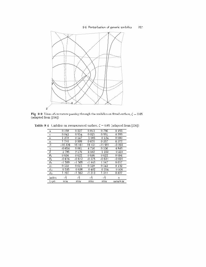
9.6 Perturbation of generic umbilics 257
x
y
z
Fig. 9.9. Lines of curvature passing through the umbilics on �tted surface, � = 0:05(adapted from [256])
Table 9.4. Umbilics on reconstructed surface, � = 0:05 (adapted from [256])
u 0.198 0.227 0.813 0.796 0.493v 0.043 0.954 0.025 0.991 0.399� 1.278 0.147 -1.005 -0.124 0.090� 1.748 0.999 0.678 0.357 6.572� -16.370 16.161 19.451 -11.981 -0.293 -0.054 0.061 4.716 0.536 4.849� -2.705 2.176 3.082 -1.233 -0.410�1 0.656 0.622 0.686 0.622 0.094�2 -0.616 -0.642 -0.575 -0.634 -0.692�3 -1.569 -1.569 -1.443 1.547 0.657�1 0.532 0.615 0.528 0.543 0.132�2 -0.535 -0.630 -0.482 -0.554 -0.856�3 1.497 -1.562 -1.513 1.544 0.827
index - 12
- 12
- 12
- 12
12
type star star star star monstar

258 9. Umbilics and Lines of Curvature
9.7 In ection lines of developable surfaces
9.7.1 Di�erential geometry of developable surfaces
A ruled surface is a curved surface which can be generated by the continu-ous motion of a straight line in space along a space curve called a directrix.This straight line is called a generator, or ruling, of the surface. A book byPottmann and Wallner [329] studies line geometry from the viewpoint of sci-enti�c computation and shows the interplay between theory and applications.Any point on a parametric ruled surface can be expressed as
r(u; v) = �(u) + v�(u) ; (9.74)
where �(u) is a directrix or base curve of the ruled surface and �(u) is a unitvector which gives the direction of the ruling at each point on the directrix.Alternatively, the surface can be represented as a ruling joining correspondingpoints on two space curves. This is represented by
r(u; v) = (1� v)rA(u) + vrB(u); 0 � u; v � 1 ; (9.75)
where rA(u) and rB(u) are directrices, as shown in Fig. 9.10. The two repre-sentations are identical if
�(u) = rA(u) and �(u) = rB(u)� rA(u) : (9.76)
directrix, rA(u)
directrix, rB (u)
generator, ruling
a0
b0
a1
b1
a2
b2
a3
b 3
Fig. 9.10. A ruled surface
A developable surface is a special ruled surface which has the same tangentplane at all points along a generator [13, 221, 120, 32, 325, 251, 328]. Since

9.7 In ection lines of developable surfaces 259
surface normals are orthogonal to the tangent plane and the tangent planealong a generator is constant, all normal vectors along a generator are parallel.This is shown in Fig. 9.11.
A developable surface has following di�erential geometry properties [411]:
1. A developable surface can be mapped isometrically onto a plane.2. Isometric surfaces have the same Gaussian curvature at corresponding
points.3. Corresponding curves on isometric surfaces have the same geodesic cur-
vature at corresponding points.4. Every isometric mapping is conformal; i.e. the angle of intersection of
every arbitrary pair of intersecting arcs on a developable surface is thesame as that of the corresponding inverse image in the plane at thecorresponding points.
5. A geodesic on a developable surface maps to a straight line in the plane.
tangent plane
generator
surface normals
Fig. 9.11. A developable surface with its tangent plane along a ruling
A developable surface can be formed by bending or rolling a planar surfacewithout stretching or tearing; in other words, it can be developed or unrolledisometrically onto a plane. Developable surfaces are also known as singlycurved surfaces, since one of their principal curvatures is zero. Developablesurfaces are widely used with materials that are not amenable to stretching.Applications include the formation of ship hulls, ducts, shoes, clothing andautomobile parts such as upholstery, body panels and windshields [120].
As indicated by Munchmeyer and Haw [280], a developable surface can beshaped purely by rolling and should be fed to the roller so that the directionof the zero principal curvature is parallel to the rolls. However, when the sheet

260 9. Umbilics and Lines of Curvature
reaches a line of in ection, it can no longer be fed into the roller in the samedirection because the direction of bending changes. Therefore, it is bene�cialfor planning the fabrication process to determine the lines of in ection priorto such a process.
Surface in ection of a developable surface was studied by Hoitsma [172]who showed that a surface has an in ection at a point p if and only if its meancurvature changes sign in the neighborhood of p. Maekawa and Chalfant [250]further extended this result and derived two theorems (Theorem 9.7.1 and9.7.2).
Since the Gaussian curvature of a developable surface is zero everywhere[411, 76], the maximum and minimum principal curvatures (3.49) and (3.50)of a developable surface can be written as
�max = H + jH j; �min = H � jH j : (9.77)
The principal curvatures reduce to
�max = 2H; �min = 0 when H > 0 ; (9.78)
�max = 0; �min = 0 when H = 0 ; (9.79)
�max = 0; �min = 2H when H < 0 : (9.80)
It is clear from (9.78) through (9.80) that at least one of the principal cur-vatures is zero at each point on a developable surface, which agrees withthe fact that the Gaussian curvature is zero everywhere (see (3.61)). �max
in (9.78) and �min in (9.80) are termed the nonzero principal curvature, ��,where �� = 2H .
In the following we establish some elementary di�erential geometry prop-erties of developable surfaces. We assume that the developable surface isregular and the u = const iso-parametric line corresponds to the generator ofthe developable surface or, in other words, the straight line ruling is in the vdirection. With this assumption, rvv = 0, and hence the second fundamentalform coe�cient (see (3.28)) N = rvv �N vanishes. From (3.46), since Gaussiancurvature of a developable surface is zero,
K =�M2
EG� F 2= 0 ; (9.81)
and hence we have M = 0. Therefore, the mean curvature (3.47) reduces to
H =�GL
2(EG� F 2): (9.82)
Recall that the nonzero principal curvature is given by �� = 2H and sinceG > 0, H and hence �� become zero if and only if L = 0, otherwise �� =2H 6= 0.
Next, we will show that the u = const parametric straight lines becomethe lines of zero curvature. This can be seen from the fact that i) the u = const

9.7 In ection lines of developable surfaces 261
iso-parametric straight lines have zero normal curvature, and ii) no other di-rection has zero normal curvature. The second fact comes from Euler's theo-rem introduced in Sect. 3.6. When �2 = 0, (3.87) reduces to � = �1 cos
2(�),which becomes zero only when � = �
2 or 3�2 , corresponding to the direction
of �2. Similarly, when �1 = 0, � = 0 only when � = 0 or �, corresponding tothe direction of �1.
Theorem 9.7.1. A developable surface does not possess generic isolated atpoints 5 but rather may contain a line of non-generic at points along agenerator [250].
Proof: From (9.79) and (9.82), L vanishes at a at point r(uf ; vf ) where bothprincipal curvatures are zero. Therefore from the �rst equation of (3.27) wehave
L(uf ; vf ) = �ru(uf ; vf ) �Nu(uf ; vf ) = 0 : (9.83)
From (9.81),M = 0 on a developable surface. Hence from the second equationof (3.27) we have
M(uf ; vf ) = �rv(uf ; vf ) �Nu(uf ; vf ) = 0 : (9.84)
Since N is a unit vector, we also have
N(uf ; vf ) �Nu(uf ; vf ) = 0 : (9.85)
If Nu is not zero, then from (9.83), (9.84) and (9.85) Nu must be perpendic-ular to ru, rv and N. This is impossible because N is perpendicular to bothru and rv , and ru is not parallel to rv . Thus, Nu(uf ; vf ) must equal zero. Fordevelopable surfaces, the unit normal vectorN is constant along a generator.Therefore, the rate of change of the unit normal vector in the u directionmust also be constant along a generator. This leads us to the fact that Nu isnot only zero at r(uf ; vf ) but also zero along the u = uf iso-parametric line.Therefore, for a given u = uf , (9.83) becomes
L(uf ; v) = �ruu(uf ; v) �N(uf ; v) = 0 ; (9.86)
for 0 � v � 1. Consequently, the entire generator consists of a line of atpoints.
For a developable surface, the in ection line is a generator which consistsof a line of at points and the nonzero principal curvature changes sign. Thein ection line can be detected by �nding u = uf such that L(uf ; vn) = 0where vn is an arbitrary constant between 0 and 1. L(u; vn) = 0 can bewritten as
5 A developable surface cannot possess spherical umbilics since one of the principalcurvatures is always zero.

262 9. Umbilics and Lines of Curvature
ruu(u; vn) � ru(u; vn)� rv(u; vn)jru(u; vn)� rv(u; vn)j = 0 : (9.87)
Since we are assuming a regular surface such that jru� rvj 6= 0, we only needto set the numerator of (9.87) equal to zero. Thus, jruu(u; vn) ru(u; vn)rv(u; vn)j = 0. For a polynomial surface with degree n in the u direction thisresults in a univariate polynomial equation of degree (3n� 4) in u
(yuzv � zuyv)xuu � (xvzu � xuzv)yuu + (xuyv � xvyu)zuu = 0: (9.88)
If the surface is expressed in a piecewise polynomial form such as a B-splinerepresentation, (9.88) must be applied to each polynomial segment separately.The univariate polynomial equation can be robustly and e�ciently solved bythe Interval Projected Polyhedron algorithm described in Chap. 4.
The local approximation (8.73) will now be applied to developable sur-faces.
Lemma 9.7.1. A developable surface is, in general, locally a parabolic cylin-der except at an in ection line, where it becomes a cubic cylinder, providedthat hxxx 6= 0 [250].
Proof: Let us consider an orthogonal Cartesian reference frame O-XY Zattached to the surface r = r(u; v) at an arbitrary point P with r(u0; v0)being P . We choose unit vectors rv
jrvj�N, rvjrvj and N at P as the directions of
X , Y and Z axes such that the Y axis coincides with the generator u = u0, theZ axis coincides with the surface normal vector and the X axis is orthogonalto both axes. Therefore the local coordinates X , Y and Z are given by
X =
�rvjrv j �N
�o
� [r(u; v)� r(uo; vo)] ; (9.89)
Y =
�rvjrv j
�o
� [r(u; v)� r(uo; vo)] ; (9.90)
Z = h(u; v) = N(uo; vo) � [r(u; v)� r(uo; vo)] ; (9.91)
where subscript o denotes that the expressions are evaluated at (uo, vo). In(9.89) through (9.91) all terms involving ru, rv and N are evaluated at (uo,vo), so r(u; v) is the only term that is a function of u and v. If we consideru and v as functions of X and Y , i.e. u = u(X;Y ) and v = v(X;Y ), thenthe height function h can be represented as a function of X and Y throughintermediate variables u and v, i.e. h(u(X;Y ); v(X;Y )).
The second fundamental form coe�cient M in terms of the height func-tion h(X;Y ) is given in (3.65) as M = hXY
(1+h2X+h2
Y)1=2
. Since M = 0 on a
developable surface (see (9.81)), we have hXY = 0. Furthermore, all the sec-ond and higher order partial derivatives with respect to Y vanish, since theY axis corresponds to the generator, which is linear in v. Thus (8.73) reducesto

9.7 In ection lines of developable surfaces 263
h(X;Y ) =1
2X2hXX(0; 0) +
1
6[X3hXXX(0; 0) + 3X2Y hXXY (0; 0)]
+R(X;Y )(jX;Y j3) : (9.92)
The second fundamental form coe�cient L in terms of the height function isgiven in (3.65) as L = hXX
(1+h2X+h2
Y)1=2
. Since L is zero along the entire generator
line, hXX and its variation in the Y direction hXXY become zero at a line ofin ection. Thus (9.92) further reduces to
h(X;Y ) =1
6(ruuu �N)
rG
EG� F 2
!3
X3 +R(X;Y )(jX;Y j3) ; (9.93)
provided that hXXX(0; 0) 6= 0. Here hXXX(0; 0) is obtained by using theinverse function theorem [76] (see Sect. 9.3) and it can be shown that ingeneral
@kh
@Xk=@kr
@uk�N r
G
EG� F 2
!k
: (9.94)
From (9.92) and (9.93) it is apparent that for small x, the quadratic termdominates except at an in ection line where the surface will become locallya cubic cylinder.When hxxx(0; 0) becomes zero, the higher order partial derivatives must beconsidered, and this is studied in the following.
A developable surface is said to have contact of order k with the tangentplane along the generator if the Taylor expansion for h(X;Y ) starts withterms of degree k + 1. The ordinary in ection line (see (9.93)) thus has acontact of order k = 2. If the tangent plane has contact of order k � 3 withthe surface along a generator, a developable surface may not look like a cubiccylinder at an in ection line.
If the developable surface has a contact of order k with the tangent plane,@ih@Xi is zero or equivalently @ir
@ui � N is zero for 1 � i � k along the entire
generator. Accordingly its variation in Y also vanishes; hence @i
@Xi@@Y h = 0
for 1 � i � k along the entire generator. Since all the second and higherorder partial derivatives with respect to Y vanish, the Taylor expansion ofthe height function along the higher order contact line reduces to
h(X;Y ) =1
(k + 1)!
�@k+1r
@uk+1�N� r
G
EG� F 2
!k+1
Xk+1
+R(X;Y )(jX;Y jk+1) : (9.95)
We can observe that for an even k the height function h(X;Y ) changes signwhen X moves across the in ection line, while for an odd k it maintains thesame sign. In other words, for an even k the height function passes through

264 9. Umbilics and Lines of Curvature
the tangent plane along the in ection line, whereas for an odd k, it liesentirely on one side of the tangent plane. Therefore in ection lines exist onlyfor even k. The order of contact can be detected by �rst solving (9.88), andsubstituting the solution into
(yuzv � zuyv)@kx
@uk� (xvzu � xuzv)@
ky
@uk+ (xuyv � xvyu)@
kz
@uk= 0 ; (9.96)
to �nd k � 3 such that (9.96) is zero for k but nonzero for k+1. The integer kfound by this process gives the order of contact (see (9.88), (9.94)). A simpleexample for the higher order odd case is given by r(u; v) = (u; v; u4)T . Sinceruu = (0; 0; 12u2)T and ru � rv = (�4u3; 0; 1)T , we can easily see that theline of at points is located at u = 0 from (9.88). And the order of contact isfound to be k = 3, since ruuu = (0; 0; 24u)T and ruuuu = (0; 0; 24)T . In thiscase the line of at points is not an in ection line, since k is odd.
9.7.2 Lines of curvature near in ection lines
At at points the principal directions are indeterminate and the orthogonalnet of lines of curvature may have singular properties. In the following weinvestigate the pattern of the lines of curvature near a line of non-generic atpoints.
Theorem 9.7.2. There is only one line of curvature that passes through each at point on a line of at points, and that line of curvature is orthogonal tothe direction of the generator [250].
Proof: By Lemma 9.7.1 the developable surface is expressed locally as acubic cylinder at an ordinary in ection line and more generally in the formof (9.95) at a higher order contact line. If we rewrite (9.95) in terms of polarcoordinates by substituting X = r cos � for a �xed radius r =
pX2 + Y 2 we
obtain
h(�) = c cosk+1 � ; (9.97)
where c is a constant evaluated at a point on the line of at points given by
c =rk+1
(k + 1)!
�@k+1r
@uk+1�N� r
G
EG� F 2
!k+1
: (9.98)
If k is even, h(� + �) = �h(�), and h(�) is an antisymmetric function of �,whereas if k is odd h(�) is a symmetric function of �. The roots of dhd� = 0 willgive the angles where local maxima and minima of h(�) may occur around the at point. The equation can be restricted to the range 0 � � < 2� withoutloss of generality. The roots are easily computed as � = 0, �2 , � and 3�
2 . Only� = 0 and � = � (which coincide with the local x axis) give extrema, since

9.7 In ection lines of developable surfaces 265
d2h(�2 )d�2 =
d2h( 3�2 )d�2 = 0. Thus � = �
2 and � = 3�2 (which coincide with the
local y axis) provide neither a maximum nor a minimum. In other words,a line of at points is not a line of curvature. Consequently, there is onlyone line of curvature passing through each at point and it is orthogonal tothe direction of the generator. For an even k the lines of maximum/minimumprincipal curvature switch to lines of minimum/maximum principal curvatureat the in ection line since h(�) is antisymmetric, while for odd k they remainthe same, since h(�) is symmetric.
If we denote � as the angle between the u axis and the direction of thenonzero principal curvature in uv parametric space, � can be evaluated asfollows. Since the direction of the nonzero principal curvature is orthogonalto the generator (parallel to the local x axis), its direction is given by rv �(ru � rv) = (rv � rv)ru � (rv � ru)rv = Gru � F rv and hence � = � tan�1 F
G .We can trace the lines of curvature which pass through the at points of an
in ection line by integrating the initial value problem following the proceduredescribed in Sect. 9.4. The starting points are obtained by slightly shiftingoutwards in the directions 0 and � from the at points or, equivalently, alongthe positive and negative local x axis.
In generic cases, umbilics are isolated [256]; thus an in ection line, whichconsists of a line of at points, is non-generic and therefore unstable. Inthe following we give a couple of numerical examples that demonstrate theinstability of the line of at points along the in ection line with respect toperturbations.
The example surface is a degree (3-1) integral B�ezier patch which is con-structed by the method developed in Chalfant [50]. The control points aregiven by
b00=(0; 0; 0)T , b01=(0:5; 0; 2)
T ,b10=(1:8; 3; 0)
T , b11=(1:895; 2:325; 2)T ,
b20=(3:3;�2; 1:5)T , b21=(3:0575;�1:55; 3:1625)T ,b30=(4; 0; 0)
T , b31=(3:6; 0; 2)T .
The surface has an ordinary in ection line at u = 0:5754, which has beencomputed by solving the degree 5 univariate polynomial equation (9.88).This surface has a net of lines of curvature which is shown in Fig. 9.12(a).Solid lines represent the lines of maximum principal curvature, while dottedlines represent the lines of minimum principal curvature. The in ection line isdepicted with a dash dotted line. Figure 9.12(b) shows a magni�cation nearthe in ection line. We can observe that there is only one line of curvaturethat passes through a at point orthogonal to the in ection line.
We gradually perturb the control points of the surface and observe thebehavior of the lines of curvature which pass through the in ection line aswe did in Sect. 9.6. Since the example is a degree (3-1) patch, it has 8 controlpoints. Each control point consists of three Cartesian coordinates x; y; z, sothere are 24 components to be perturbed. We gradually increase the pertur-bation by increasing � in (9.73) from 0:02 to 0:08 in steps of 0:02.

266 9. Umbilics and Lines of Curvature
x
y
z
inflection line
(a) (b)
Fig. 9.12. (a) Lines of curvature of developable surface with in ection, (b) mag-ni�cation near in ection line (adapted from [256])
x
y
z
(a) (b)
Fig. 9.13. (a) Lines of curvature on perturbed surface � = 0:08, (b) magni�cationnear u=0.57 (adapted from [256])
Figure 9.13 illustrates the behavior of the lines of curvature when thecontrol points are perturbed (� = 0:08). We can see from the �gure that theentire in ection line, which consists of a line of at points, disappears. Hencethere is no singularity in the net of lines of curvature when a perturbationis induced. The nonzero principal curvatures on both sides of the formerin ection line 6 meet at right angles near the former in ection line and makea very sharp change in direction (almost a right angle).
6 Once the control points are perturbed both principal curvatures may not benonzero, but here we are referring to the nonzero principal curvature beforeperturbation.
10. Geodesics
10.1 Introduction
Computation of shortest paths on free-form surfaces is an important prob-lem in geometric design of ship hulls, robot motion planning, computation ofmedial axis transforms of trimmed surface patches, terrain navigation, NCmachining, and cable installation on the sea oor. The history of geodesiclines begins with a study by Johann Bernoulli, who solved the problem ofthe shortest distance between two points on a convex surface in 1697, ac-cording to Struik [411]. He showed that the osculating plane of the geodesicline must always be perpendicular to the tangent plane. The equation ofgeodesics for implicit surfaces was �rst obtained by Euler (1732). His atten-tion to the problem was due to Johann Bernoulli, probably through the aidof his nephew Daniel, who was at St. Petersburg with Euler [410]. Bliss [28]obtained the geodesic lines on the anchor ring, which has a torus shape, an-alytically. Munchmeyer and Haw [280] applied geodesic curves to geometricdesign of ship hulls, namely to �nd out the precise layout of the seams andbutts on a ship hull. Beck et al. [22] performed both initial-value integra-tion and boundary-value integration (based on shooting method) of geodesicpaths, using the fourth order Runge-Kutta method on a bicubic spline sur-face. Patrikalakis and Bardis [295] computed geodesic o�sets of curves onrational B-spline surfaces using the initial-value integration of geodesics nor-mal to an initial progenitor curve on the surface. One application of sucho�sets is automated construction of linkage curves for free-form proceduralblending surfaces. Sneyd and Peskin [397] investigated the computation ofgeodesic paths on a generalized cylinder based on an initial value problemusing a second order Runge-Kutta method. Their work was motivated by con-structing the great vessels of the heart out of geodesic �bers. Kimmel et al.[199] presented a numerical method for �nding the shortest path on surfacesby calculating the propagation of an equal geodesic-distance contour from apoint or a source region on the surface. The algorithm works on a rectangu-lar grid using �nite di�erence approximations. Maekawa [246] and Robinsonand Armstrong [346] computed the geodesics by discretizing the governingdi�erential equations using a �nite di�erence approximation on a mesh ofpoints, which reduces the problem to a set of nonlinear equations. The set ofnonlinear equations can be solved by quadratically convergent Newton iter-

268 10. Geodesics
ation method, which starts with an initial guess and improves the solutioniteratively. This technique is referred as, direct method, relaxation method or�nite di�erence method. The shortest path problem is also very active amongthe robot motion planning and terrain navigation communities, however theyusually represent the surface as a polyhedral surface and solve the problemusing techniques from the �eld of computational geometry [268].
A geodesic path is sometimes de�ned as the shortest path between twopoints on a surface; however this is not always a satisfactory de�nition. Inthis book we follow Struik [411] and de�ne geodesics as below:
De�nition 10.1.1. Geodesics are curves of zero geodesic curvature.
In other words, the osculating planes of a geodesic curve on a surface containthe surface normal. From this de�nition we can easily see that the geodesicbetween two points on a sphere is a great circle. But there are two arcsof a great circle between two such points, and only one of them providesthe shortest distance, except when the two points are the end points of adiameter of the sphere. This example indicates that there may exist morethan one geodesics between two points on a surface.
Let Q(t) describe a moving point on a surface where t may be viewed asa time parameter belonging to an interval beginning with t0, and Q[t0; t1]describe the path between points Q(t0) and Q(t1). If the point Q(t) movesaway from the starting point Q(t0) along a geodesic path C, i.e. curve withzero geodesic curvature, then it may occur that Q(t) will reach a point Q(tR)such that for every " > 0 the path Q[t0; tR + "] is no longer the shortestsurface path joining the points Q(t0) and Q(tR + "). In other words, Q(tR)was the last time point such that the geodesic path Q[t0; tR] is the shortestsurface path joining the points Q(t0) and Q(tR). This point Q(tR) is calledconjugate toQ(t0) on the geodesic C (see also [448]). The location, where eachextension of a shortest geodesic fails to de�ne a shortest path from Q(t0),belongs to the cut locus of the point Q(t0) on the surface. This geometriclocus and its generalizations (being important for considerations on shortestpaths and geodesic distance) have been studied in [446, 448].
10.2 Geodesic equation
10.2.1 Parametric surfaces
We assume that the given parametric surface r=r(u; v) is a regular and non-periodic NURBS surface patch. Wolter [447] shows that on a regular NURBSsurface patch there always exists a shortest path joining any two patch points.If the surface patch is de�ned on a rectangular or even more generally on alocally convex planar domain, then any shortest path in the patch joiningany two patch points must have a continuous tangent with the path beingarc length parametrized. If the shortest path (without its end points) does not

10.2 Geodesic equation 269
meet the patch boundary then this shortest path is a geodesic in the sense ofDe�nition 10.1.1 where this is proven in [447] under very weak assumptions.We shall henceforth assume throughout this chapter that the shortest pathto be computed will not meet the patch boundary except possibly at its endpoints.
Let C be an arc length parametrized regular curve on this surface whichpasses through point P as shown in Fig. 3.6 and denoted by
r(s) = r(u(s); v(s)) : (10.1)
Let t be a unit tangent vector of C at P , n be a unit normal vector of Cat P , N be a unit surface normal vector of S at P and u be a unit vectorperpendicular to t in the tangent plane of the surface, de�ned by u =N� t.The u component of the curvature vector k of r(s) is the geodesic curvaturevector kg and is given by
kg = (k � u)u : (10.2)
The scalar function
�g = k � u ; (10.3)
is called the geodesic curvature of C at P , or equivalently
�g =dt
ds� (N� t) : (10.4)
The unit tangent vector of the curve C can be obtained by di�erentiating(10.1) with respect to the arc length using the chain rule
t =dr(u(s); v(s))
ds= ru
du
ds+ rv
dv
ds: (10.5)
Thus we have
dt
ds= ruu
�du
ds
�2
+ 2ruvdu
ds
dv
ds+ rvv
�dv
ds
�2
+ rud2u
ds2+ rv
d2v
ds2; (10.6)
and hence substituting (10.5) and (10.6) into (10.4) yields
�g =
"(ru � ruu)
�du
ds
�3
+ (2ru � ruv + rv � ruu)�du
ds
�2dv
ds
+(ru � rvv + 2rv � ruv)duds
�dv
ds
�2
+ (rv � rvv)�dv
ds
�3#�N
+(ru � rv) �N�du
ds
d2v
ds2� d2u
ds2dv
ds
�: (10.7)

270 10. Geodesics
We can easily observe that the coe�cients of�duds
�3,�duds
�2 dvds ,
duds
�dvds
�2,�dvds
�3,�
duds
d2vds2 � d2u
ds2dvds
�are all functions of the coe�cients of the �rst fundamen-
tal form E, F and G and their derivatives, Eu, Fu, Gu, Ev , Fv , Gv . It isinteresting to note that the normal curvature �n depends on both the �rstand second fundamental forms, while the geodesic curvature depends only onthe �rst fundamental form. Using the Christo�el symbols � i
jk (i; j; k = 1; 2)de�ned as follows [411]
� 111 =
GEu � 2FFu + FEv2(EG� F 2)
; � 211 =
2EFu �EEv + FEu2(EG� F 2)
;
� 112 =
GEv � FGu
2(EG� F 2); � 2
12 =EGu � FEv2(EG� F 2)
; (10.8)
� 122 =
2GFv �GGu + FGv
2(EG� F 2); � 2
22 =EGv � 2FFv + FGu
2(EG� F 2);
geodesic curvature reduces to
�g =
"� 211
�du
ds
�3
+ (2� 212 � � 1
11)
�du
ds
�2dv
ds+ (� 2
22 � 2� 112)
du
ds
�dv
ds
�2
�� 122
�dv
ds
�3
+du
ds
d2v
ds2� d2u
ds2dv
ds
#pEG� F 2 : (10.9)
According to the de�nition, we can determine the di�erential equation thatany geodesic on a surface must satisfy by simply setting �g = 0 in (10.9) andobtain
du
ds
d2v
ds2� d2u
ds2dv
ds= �� 2
11
�du
ds
�3
� (2� 212 � � 1
11)
�du
ds
�2dv
ds
+(2� 112 � � 2
22)du
ds
�dv
ds
�2
+ � 122
�dv
ds
�3
: (10.10)
Alternatively, we can derive the di�erential equation for geodesics by con-sidering that the surface normal N has the direction of a normal to thegeodesic curve �n
n � ru = 0; n � rv = 0 : (10.11)
Since kn = dtds , (10.11) can be rewritten as
dt
ds� ru = 0;
dt
ds� rv = 0 : (10.12)
By substituting (10.6) into equations (10:12) we have

10.2 Geodesic equation 271
(ruu � ru)�du
ds
�2
+ 2(ruv � ru)duds
dv
ds+ (rvv � ru)
�dv
ds
�2
+ Ed2u
ds2+ F
d2v
ds2= 0 ; (10.13)
(ruu � rv)�du
ds
�2
+ 2(ruv � rv)duds
dv
ds+ (rvv � rv)
�dv
ds
�2
+ Fd2u
ds2+G
d2v
ds2= 0 : (10.14)
By eliminating d2vds2 from (10.13) using (10.14), and eliminating d2u
ds2 from(10.14) using (10.13) and employing the Christo�el symbols, we obtain [411]
d2u
ds2+ � 1
11
�du
ds
�2
+ 2� 112
du
ds
dv
ds+ � 1
22
�dv
ds
�2
= 0 ; (10.15)
d2v
ds2+ � 2
11
�du
ds
�2
+ 2� 212
du
ds
dv
ds+ � 2
22
�dv
ds
�2
= 0 : (10.16)
Equations (10.15) and (10.16) are related by the �rst fundamental form ds2 =Edu2 + 2Fdudv + Gdv2 and if we eliminate ds from both equations, theequations reduce to (10.10) with u taken as parameter. These two secondorder di�erential equations can be rewritten as a system of four �rst orderdi�erential equations [234]
du
ds= p ; (10.17)
dv
ds= q ; (10.18)
dp
ds= �� 1
11p2 � 2� 1
12pq � � 122q
2 ; (10.19)
dq
ds= �� 2
11p2 � 2� 2
12pq � � 222q
2 : (10.20)
We can also �nd this result by means of the general rules of the calculusof variations [166]. We want to minimize
I =
Z B
A
ds =
Z B
A
sE + 2F
dv
du+G
�dv
du
�2
du =
Z B
A
f(u; v; _v)du ;
(10.21)
subject to the conditions
v(A) = vA; v(B) = vB ; (10.22)
where
272 10. Geodesics
f(u; v; _v) =pE + 2F _v +G _v2; _v =
dv
du; (10.23)
and vA and vB are given constants. It is well known from calculus of variationsthat the solution of Euler's equation [166]
@f
@v� d
du
@f
@ _v= 0 ; (10.24)
gives an extreme value to the integral (10.21). When (10.23) is substituted inEuler's equation (10.24) we can derive the di�erential equation for geodesics.
Example 10.2.1. Let us obtain the geodesic equations for a parametric bi-linear surface (hyperbolic paraboloid) r(u; v) = (u; v; uv) (see Fig. 3.4). Wehave
E = 1 + v2; F = uv; G = 1 + u2 ;Eu = 0; Fu = v; Gu = 2u ;Ev = 2v; Fv = u; Gv = 0 ;
thus, the Christo�el symbols become
� 111 = � 2
11 = � 122 = � 2
22 = 0 ;
� 112 =
v
u2 + v2 + 1;
� 212 =
u
u2 + v2 + 1:
Finally the geodesic equations for the bilinear surface are given by
du
ds= p ;
dv
ds= q ;
dp
ds=
�2vu2 + v2 + 1
pq ;
dq
ds=
�2uu2 + v2 + 1
pq :
10.2.2 Implicit surfaces
We can also derive the geodesic equation for an implicit surface by �nding anexpression of the geodesic curvature for an implicit surface. Let us consideran arc length parametrized curve r = r(s) or x = x(s), y = y(s), z = z(s)on an implicit surface f(x; y; z) = 0. By substituting t = (x0; y0; z0)T , dt
ds =
(x00; y00; z00)T ,N = rfjrf j , into (10.4), we obtain the expression for the geodesic
curvature of a curve on the implicit surface

10.2 Geodesic equation 273
�g =(y0z00 � z0y00)fx + (z0x00 � x0z00)fy + (x0y00 � y0x00)fzq
f2x + f2y + f2z
: (10.25)
For the sake of completeness, the geodesic curvature for a non-arc-lengthparametrized curve is given by
�g =( _y�z � _z�y)fx + ( _z�x� _x�z)fy + ( _x�y � _y�x)fz
( _x2 + _y2 + _z2)32
qf2x + f2y + f2z
: (10.26)
Now if we set �g = 0, we deduce
(y0z00 � z0y00)fx + (z0x00 � x0z00)fy + (x0y00 � y0x00)fz = 0 : (10.27)
Since the unit tangent vector (x0; y0; z0) and the curvature vector (x00; y00; z00)of the geodesic curve are orthogonal to each other, we have
x0x00 + y0y00 + z0z00 = 0 : (10.28)
The third equation can be derived from (6.21)
fxx(x0)2 +fyy(y
0)2 + fzz(z0)2 + 2(fxyx
0y0 + fyzy0z0 + fxzx
0z0)
+fxx00 + fyy
00 + fzz00 = 0 : (10.29)
Now we solve the linear system of three equations (10.27) to (10.29) in(x00; y00; z00), assuming that (z0fy � y0fz)2 + (x0fz � z0fx)2 + (y0fx � x0fy)2does not vanish, yielding
x00 =(x0fz � z0fx)z0 + (x0fy � y0fx)y0
(z0fy � y0fz)2 + (x0fz � z0fx)2 + (y0fx � x0fy)2� ; (10.30)
y00 =(y0fz � z0fy)z0 + (y0fx � x0fy)x0
(z0fy � y0fz)2 + (x0fz � z0fx)2 + (y0fx � x0fy)2� ; (10.31)
z00 =(z0fy � y0fz)y0 + (z0fx � x0fz)x0
(z0fy � y0fz)2 + (x0fz � z0fx)2 + (y0fx � x0fy)2� ; (10.32)
where � = fxx(x0)2+fyy(y0)2+fzz(z0)2+2(fxyx
0y0+fyzy0z0+fxzx0z0). Thesethree second order di�erential equations can be rewritten as a system of six�rst order di�erential equations:
x0 = p ; (10.33)
y0 = q ; (10.34)
z0 = r ; (10.35)
p0 =(pfz � rfx)r + (pfy � qfx)q
(rfy � qfz)2 + (pfz � rfx)2 + (qfx � pfy)2� ; (10.36)
q0 =(qfz � rfy)r + (qfx � pfy)p
(rfy � qfz)2 + (pfz � rfx)2 + (qfx � pfy)2� ; (10.37)
r0 =(rfy � qfz)q + (rfx � pfz)p
(rfy � qfz)2 + (pfz � rfx)2 + (qfx � pfy)2� : (10.38)

274 10. Geodesics
Figure 10.1 shows a geodesic on an ellipsoid (x2
9 + y2
4 + z2 = 1) computedby integrating the above system of six �rst order di�erential equations asan initial value problem. The initial values are given by (x; y; z) = (0, 2, 0),
(p; q; r)=�p
22 ; 0;
p22
�and the integration is terminated at (x; y; z)=(2.439,
-0.726, 0.456).
−4
−2
0
2
4
−2−1
01
2
−1
−0.8
−0.6
−0.4
−0.2
0
0.2
0.4
0.6
0.8
1
Fig. 10.1. Geodesics on an ellipsoid
10.3 Two point boundary value problem
10.3.1 Introduction
We can solve the system of four �rst order ordinary di�erential equations(10.17) to (10.20) as an initial value problem (IVP), where all four boundaryconditions are given at one point, or as a boundary value problem (BVP),where four boundary conditions are speci�ed at two distinct points. Most ofthe problems that arise in applications of geodesics are not IVP but BVP,which are much more di�cult to solve. It is well known that the solutionof an IVP is unique, however for a BVP it is possible that the di�erentialequations have many solutions or even no solution [193]. General methodsfor the solutions of two-point BVPs can be found in [193, 117].
It is convenient to write the system of di�erential equations in vectorform, since we can describe the equations for systems in terms of a single
10.3 Two point boundary value problem 275
vector equation. Let us set
y = (y1; y2; : : : ; yn)T ; g = (g1; g2; : : : ; gn)
T ;� = (�1; �2; : : : ; �n)
T ; � = (�1; �2; : : : ; �n)T ;
s 2 [A;B] ;(10.39)
where yi, gi are functions and �i, �i are constants. Then the general �rst ordervector di�erential equation for a boundary value problem can be written as:
dy
ds= g(s;y); y(A) = �; y(B) = � : (10.40)
There are two commonly used approaches to the numerical solution ofBVPs. The idea of the �rst technique is that if all values of y(s) are knownat s = A, then the problem can be reduced to an IVP. However, y(A) can befound only by solving the problem. Therefore an iterative procedure must beused. We assume values at s = A, which are not given as boundary conditionsat s = A and compute the solution of the resulting IVP to s = B. Thecomputed values of y(B) will not, in general, agree with the correspondingboundary condition at s = B. Consequently, we need to adjust the initialvalues and try again. The process is repeated until the computed values at the�nal point agree with the boundary conditions and is referred to as shootingmethod. The second method is based on a �nite di�erence approximation todyds on a mesh of points in the interval [A;B]. This method starts with aninitial guess and improves the solution iteratively and is referred to as, directmethod, relaxation method or �nite di�erence method. We have implementedboth methods and found that the �nite di�erence method is much morereliable than the shooting method. By contrast to the �nite di�erence method,the shooting method is often very sensitive to the unknown initial values atpoint A. First, we brie y discuss the shooting method.
10.3.2 Shooting method
We assume a value for pA and solve the di�erential equation as an IVPusing the fourth order Runge-Kutta method. Using the �rst fundamentalform (3.13), given pA we can obtain qA from
qA =�FpA �
pF 2p2A �G(Ep2A � 1)
G: (10.41)
Here we also have to assume the entire arc length of the geodesic path sto stop the integration. Thus the unknowns can be considered as pA and s.If we denote the computed value of (uB ; vB) as (u
�B ; v
�B), the di�erence can
be given as (u�B � uB; v�B � vB). We need to adjust pA and s to make thedi�erence zero. This can be done by employing Newton's method�
pAs
�i+1
=
�pAs
�i
�"@u�B@pA
@u�B@s
@v�B@pA
@v�B@s
#�1
i
�u�B � uBv�B � vB
�; (10.42)
276 10. Geodesics
where the Jacobian matrix is evaluated numerically. We �rst change pAslightly to pA + �pA and integrate the ordinary di�erential equations asan IVP to evaluate the end point (u�B(pA +�pA; s); v
�B(pA +�pA; s)), from
which we can compute the partial derivatives@u�B@pA
and@v�B@pA
as
@u�B@pA
=u�B(pA +�pA; s)� u�B(pA; s)
�pA; (10.43)
@v�B@pA
=v�B(pA +�pA; s)� v�B(pA; s)
�pA: (10.44)
Similarly we change s slightly to s+�s and integrate the ordinary di�erentialequations as IVP to evaluate the end point (u�B(pA; s+�s); v
�B(pA; s+�s)),
from which we can compute the partial derivatives@u�B@s and
@v�B@s
@u�B@s
=u�B(pA; s+�s)� u�B(pA; s)
�s; (10.45)
@v�B@s
=v�B(pA; s+�s)� v�B(pA; s)
�s: (10.46)
10.3.3 Relaxation method
The relaxation method [335, 246] starts by �rst discretizing the governingequations by �nite di�erences on a mesh with m points. The computationbegins with an initial guess and improves the solution iteratively or in otherwords relaxes to the true solution. Let us consider an arc length parametrizedcurve connecting A and B on the surface with a mesh of points satisfyingA = s1 < s2 < : : : < sm = B. We approximate the n �rst order di�erentialequations by the trapezoidal rule [117]
Yk �Yk�1
sk � sk�1=
1
2[Gk +Gk�1]; k = 2; 3; : : : ;m ; (10.47)
with boundary conditions
Y1 = �; Ym = � : (10.48)
Here the n-vectorsYk,Gk are meant to approximate y(sk) and g(sk).Y1 hasn1 known components, while Ym has n2 = n� n1 known components. Thisdiscrete approximation will be accurate to the order of h2 (h = maxkfsk �sk�1g). Equation (10.47) forms a system of (m � 1)n nonlinear equationswith mn unknowns Yk = (Y1; Y2; : : : ; Yn)
Tk (k = 1; : : : ;m). The remaining n
equations come from boundary conditions (10.48). Let us refer to (10.47) as
Fk = (F1;k; F2;k; : : : ; Fn;k)T =
Yk �Yk�1
sk � sk�1� 1
2[Gk +Gk�1] = 0 ;
(10.49)

10.4 Initial approximation 277
where k = 2; 3; : : : ;m, and refer to (10.48) as
F1 = (F1;1; F2;1; : : : ; Fn1;1)T = Y1 �� = 0 ;
Fm+1 = (F1;m+1; F2;m+1; : : : ; Fn2;m+1)T = Ym � � = 0 ; (10.50)
then we have mn nonlinear equations
F = (FT1 ;FT2 ; : : : ;F
Tm+1)
T = 0 : (10.51)
This system of nonlinear equations can be solved by quadratically con-vergent Newton iteration, if a su�ciently accurate starting vector Y(0) =(YT
1 ;YT2 ; : : : ;Y
Tm)
T is provided. The Newton iteration scheme is given by
Y(i+1) = Y(i) +�Y(i) ; (10.52)
[J(i)]�Y(i) = �F(i) ; (10.53)
where superscripts (i) denote i-th iteration and [J(i)] is the mn by mn Jaco-bian matrix of F(i) with respect to Y(i).
Since the corrections are based on a �rst order Taylor approximation, theusual Newton method may not be su�cient for a complex nonlinear problemunless a good initial approximation is provided. If the vector norm of thecorrection vector is large, then it is an indication that the problem is highlynonlinear and may produce a divergent iteration. To achieve more stabilitywe can employ a step correction procedure
Y(i+1) = Y(i) + ��Y(i) ; (10.54)
where 0 < � � 1 chosen so that k �Y(i+1) k1 < k �Y(i) k1, where k �Y k1is a scaled vector norm and de�ned as
k �Y k1=mXk=1
� j�ukjMu
+j�vkjMv
+j�pkjMp
+j�qkjMq
�; (10.55)
where Mu, Mv, Mp and Mq are the scale factors for each variable. Maekawa[246] usedMu=Mv=1 andMp=Mq=10, since the magnitude of �pk and �qkare roughly ten times larger that of �uk and �vk as numerical experimentshave shown. If � = 1 the equation reduces to the usual Newton's method,while if � < 1 the rate of convergence will be less than quadratic. Newton'smethod terminates when the norm of the solution vector is smaller than thepre-speci�ed tolerance "N . The order of "N should be proportional to h2,since we are using the trapezoidal rule (see (10.47)).
10.4 Initial approximation
10.4.1 Linear approximation
Linear approximation is the simplest and most often provides a good initialapproximation, since it is a solution to the system of geodesic equations

278 10. Geodesics
(10.17) to (10.20) when we neglect all the nonlinear terms in the right handside. We connect the two end points in the parameter space by a straight lineand de�ne a uniform mesh or grid by a set of k = 1; 2; : : : ;m points as shownin Fig. 10.2 (a). Therefore we have
uk = uA +uB � uAm� 1
(k � 1) ; (10.56)
vk = vA +vB � vAm� 1
(k � 1) : (10.57)
When the uniform mesh in the parameter space is mapped onto the surface,the corresponding arc length mesh will not be in general uniform.
A
C
D
B
(uA,vA)
(uB,vB)
k=m
Ak=1
B
u
v
u
v
(uA,vA)
k=1
k=m(uB,vB)
(b)(a)
(uC,vC)
(uD,vD)
Fig. 10.2. Initial approximations (adapted from [246]): (a) linear approximation,(b) circular arc approximation
If we assume that uA 6= uB then
dv
du=vB � vAuB � uA � � ; (10.58)
hence
dv
ds= �
du
ds: (10.59)
By substituting this relation into the �rst fundamental form we obtain
E
�du
ds
�2
+ 2F�
�du
ds
�2
+G�2�du
ds
�2
= 1 : (10.60)

10.4 Initial approximation 279
Thus
pk =du
ds= � 1p
Ek + 2Fk�+Gk�2; (10.61)
qk =dv
ds= � �p
Ek + 2Fk�+Gk�2: (10.62)
When uA = uB, it is easy to �nd that pk = 0 and qk =1pGk
. It is well known
that conjugate points do not exist on regions of a surface where the Gaussiancurvature is negative [411]. Therefore, the linear approximation will typicallyprovide a good initial approximation to the geodesic path in those regions.
10.4.2 Circular arc approximation
The problem of the straight line approximation is that when there are morethan one path, it cannot capture the other paths. To make the method morereliable, the following algorithm has been developed [246]. First we pick twopoints C and D in the parameter domain, which are on the bisector of thetwo end points A and B, such that AC = AD or BC = BD as illustrated inFig. 10.2 (b). Then we determine two circular arcs which pass through thethree points A;C;B and A;D;B. If C and D are taken at a large enoughdistance from AB, all the geodesic paths in the parameter domain betweenpoints A and B are likely to lie within or close to the region surrounded bythe two circular arcs. Notice that the algorithm fails once the circular arcsgo outside the domain so these arcs are chosen such that they are entirelywithin the domain. The uv coordinates in the parameter domain i.e. (uk; vk),k = 1; : : : ;m can be obtained by equally distributing the points along thecircular arc in the parameter domain. Once we have a set of points in theparameter domain, we can easily evaluate pk; qk by using the central di�erenceformula for a non-uniform mesh points [117], for k = 2; : : : ;m� 1
f 0(sk) =hkhk+1
(fk+1 � fk)� hk+1
hk(fk�1 � fk)
hk + hk+1; (10.63)
the forward di�erence formula for k = 1
f 0(s1) =�h2h3f3 +
�h2h3
+ h3h2
+ 2�f2 �
�2 + h3
h2
�f1
h2 + h3; (10.64)
and the backward di�erence formula for k = m
f 0(sm) =hmhm�1
fm�2 ��hm�1
hm+ hm
hm�1+ 2�fm�1 +
�2 + hm�1
hm
�fm
hm�1 + hm;
(10.65)

280 10. Geodesics
where f is replaced by u or v, and the step length hk = sk�sk�1 is evaluatedby computing the chord length between the successive points on the surface.Even if the mesh points are equally distributed along the circular arc in theparameter domain as shown in Fig. 10.2 (b), hk is not in general constant.
We give the ow chart of the algorithm based on circular arc approxi-mation for computing the geodesic path between two given points in Fig.10.3.
10.5 Shortest path between a point and a curve
In this section we solve a problem of �nding a shortest path between a pointand a curve on a free-form non-periodic parametric surface [246], which uti-lizes the method we have developed in Sects. 10.3 and 10.4. This conceptis important in robot motion planning and constructing a medial axis ona free-form surface. Suppose we have a point A and a curve C on a para-metric surface r(u; v) de�ned as rc(t) = r(uc(t); vc(t)), we want to computethe shortest path between point A and curve C as shown in Fig. 10.4. Theexistence of such a shortest path follows from results shown in [447]. Let usdenote the intersection point of the curve C and the shortest path by B.Wolter [448] developed a necessary condition to have a shortest path frompoint A to curve C, provided that the point B is not an end point of thecurve C. The condition is given by the orthogonality of the tangent vector ofthe geodesic curve, connecting A and C, at B and the tangent vector of Cat B. If point B were known, the problem could be reduced to an IVP, sinceat point B, u, v, p and q are all known. However, point B can be found onlyby solving the problem. We guess a parameter value t = tB for point B andsolve the BVP. In general the unit tangent vector of the curve rc(t) and theunit tangent vector of the arc length parametrized geodesic curve rg(s) at theguessing point will not be orthogonal to each other. Consequently, we needto adjust the parameter value tB and iterate until those two unit tangentvectors become orthogonal. Therefore for each iteration, we need to solve atwo point boundary value problem, which also requires iterations (i.e., nestediteration). If we denote these two unit tangent vectors as tc and tg , then theycan be expressed as follows:
tc =drc(t)dt���drc(t)dt
��� =ru
duc
dt + rvdvc
dtq(du
c
dt xu +dvc
dt xv)2 + (du
c
dt yu +dvc
dt yv)2; (10.66)
tg =drg(s)
ds= ru
dug
ds+ rv
dvg
ds: (10.67)
Therefore the orthogonality condition can be written as
!(t) = tc � tg

10.5 Shortest path between a point and a curve 281
Solve the BVP and denote the solution vectors by (L, R)
|L − R|<ε
Add L and R to the solution list and push (L,R) into stack S
Add L to the solution list
Start with two circular arc approximations (YL, YR) as initial vectors
Yes
NoEnd
|L − R|<ε Add L to the solution list
Compute a new approximation vector YM by taking the mid points of L and R, i.e. YM=(L+R)/2
Solve the BVP with YM as input and denote the output by M
|L − M|<ε or M moves further left to L
|R − M|<ε or M moves further right to R
Push (YM,R) to stack S
Push (L,YM) to stack S
Yes
Yes
Yes
No
No
No
Pop (L,R) from stack S
We add M to the solution list and push (L,M) and (M,R) to stack S
Stack S is empty
End
No
Yes
Find the shortest path from the list of solution vectors
Fig. 10.3. Flow chart of the algorithm based on circular arc approximation forcomputing the geodesic path between two given points (adapted from [246])

282 10. Geodesics
.
.
A
B
C
S
tg
tc
rc(t)
rg(s)
Fig. 10.4. Shortest path between point A and curve C (adapted from [246])
=dug
dsduc
dt E + (dvg
dsduc
dt + dvc
dtdug
ds )F + dvg
dsdvc
dt Gq(du
c
dt xu +dvc
dt xv)2 + (du
c
dt yu +dvc
dt yv)2
= 0 : (10.68)
Consequently we need to �nd a parameter value tB such that !(tB) = 0.Since the relationship described above is implicit, we use the secant method[69] instead of Newton's method to obtain tB . The secant method can be de-
rived from Newton's method by replacing the derivative d!(i)
dt by the quotient
(!(i)�!(i�1))=(t(i)�t(i�1)) where superscripts (i) denote i-th iteration. Thisleads to the following scheme
t(i+1) = t(i) +�t(i); �t(i) = � t(i) � t(i�1)
!(i) � !(i�1)!(i); !(i) 6= !(i�1) :
(10.69)
Notice that the secant method requires two initial approximations t(1) andt(2). Since the secant method has an order of convergence of 1
2 (1+p5) ' 1:618
[69], it converges within a reasonable number of iterations. If the correction�t(i) is large, it is again an indication that the problem is highly nonlinear.In such case we also employ a step correction procedure
t(i+1) = t(i) + ��t(i) ; (10.70)
where � is a correction factor 0 < � � 1, determined as for the modi�edNewton's method. Since we do not know how many solutions exist and thecorresponding parameter values of the curve beforehand, we can use a similar

10.6 Numerical applications 283
algorithm to the circular arc approximation. If the range of the parametervalue of the curve is 0 � t � 1, we start from both ends of the curve (i.e.t(1)=0, t(2)=0.02 and t(1) = 1, t(2)=0.98). Then we recursively �nd the so-lutions. Although we may have several footpoints B in di�erent locations ofthe curve, for each footpoint there is only one unique solution between A andB, since this can be viewed in the context of an initial value problem.
10.6 Numerical applications
10.6.1 Geodesic path between two points
The �rst example is a wave-like bicubic B-spline surface, whose control poly-hedron is a lattice of 7�7 vertices with uniform knot vectors in both directionsand spans 0 � x � 1, 0 � y � 1. Let us compute the geodesic path betweentwo corner points, (uA, vA)= (0,0) and (uB , vB)=(1,1). We choose (uC ; vC)to be (0.7, 0.3) and (uD; vD) to be (0.3, 0.7) for the circular arc approxima-tion. The algorithm based on circular arc approximation �nds three geodesicpaths, as shown in Fig. 10.5 (solid thick lines). The computational condi-tions such as number of mesh points, tolerance and correction factor for theNewton's method "N , �, as well as computational results such as number ofiterations for convergence and the geodesic distances are listed in Table 10.1.Symbols Lt, Md, Rt refer to left, middle and right geodesic paths in Fig.10.5. The middle geodesic path is not a minimal path (s=1.865), while theother two paths are the shortest path (s = 1:661) due to symmetry. Figure10.6 shows how the initial approximation path (the right-most thick solidline) converges gradually to the �nal solution (wavy thick solid line). Theintermediate paths are illustrated by the thin solid lines.
Table 10.1. Numerical conditions and results for the computation of the geodesicpath between corner points of the wave-like surface (adapted from [246])
Points Tolerance Correction Iterations Geodesic distancem "N factor � Lt Md Rt Lt Md Rt101 1.0E-3 0.2 22 1 22 1.661 1.865 1.661
The second example is a generalized cylinder represented by a biquadraticrational B-spline surface, whose control polyhedron is a lattice of 6�9 vertices.This surface was constructed by sweeping a circle of radius 0.5, the generatrix,along a helix (x = cos t, y = � sin t, z = t
� , 0 � t � 2�), the spine, and isapproximated by rational B-spline interpolating a number of generatrices.When we keep u constant, we obtain a curve on the surface which dependsonly on v. This curve coincides with the generatrix. Similarly v = constant

284 10. Geodesics
x
y
z
Fig. 10.5. Geodesic paths on the wave-like bicubic B-spline surface between pointsof two corners (adapted from [246])
represents another iso-parametric curve which is parallel to the spine. Twoend points are chosen to be (uA; vA)=(0, 0.4) and (uB ; vB)=(1, 0.6) as shownin Fig. 10.7. In Fig. 10.7 three initial approximations are illustrated by thethin solid lines, while the �nal solutions are illustrated by the thick solid lines.The two circular arcs are determined by setting (uC ; vC) = (0.578, 0.108),(uD; vD) = (0.422, 0.892). The circular arc approximation algorithm startswith these two circular arcs and converges to the two minimal geodesic pathswhich are shown as thick solid lines close to the initial circular arcs. Theminimal geodesic paths mapped onto the generalized cylinder are depicted inColor Plate A.8 and Fig. 10.8. Then the algorithm computes the mid-pointsof these solutions, which is shown as a thin straight line connecting the twoend points. This initial approximation converges to a sine wave-like solution.This solution is a geodesic path but it does not provide the shortest distance(see Fig. 10.9). Table 10.2 shows the list of computational conditions andresults as in Table 10.1.
10.6.2 Geodesic path between a point and a curve
Figure 10.10 shows a planar cubic B�ezier curve and point A (0.3, 0.2) in the uvparameter domain, which will be mapped onto the wave-like B-spline surface

10.6 Numerical applications 285
x
y
z
Fig. 10.6. Convergence of the right geodesic path in Fig. 10.5 (adapted from [246])
Table 10.2. Numerical conditions and results for the computation of the geodesicpath between two points on generalized cylinder (adapted from [246])
Points Tolerance Correction Iterations Geodesic distancem "N factor � Lt Md Rt Lt Md Rt501 1.0E-2 0.2 8 10 8 5.860 6.983 5.8601001 5.0E-3 0.2 10 10 10 5.843 6.956 5.843
as shown in Fig. 10.11. The algorithm �nds three geodesic paths AB, AB0 andAB00, whose tangent vectors at B, B0 and B00 are orthogonal to the tangentvectors at the curve at those points. Table 10.3 shows the list of computationalconditions and results. The entries t1, t2 and tB are the parameter valuesof the curve corresponding to the �rst two initial approximations for thesecant method and the solution value. The following entries, m, � and � arethe number of mesh points, correction factors for the Newton and secantmethods. Tolerances for the convergence of Newton and secant methods aregiven by "N , "S . The shortest path is given by path AB with s=0.275.
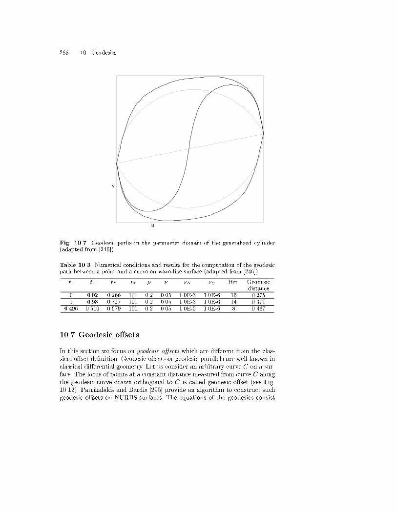
286 10. Geodesics
u
v
Fig. 10.7. Geodesic paths in the parameter domain of the generalized cylinder(adapted from [246])
Table 10.3. Numerical conditions and results for the computation of the geodesicpath between a point and a curve on wave-like surface (adapted from [246])
t1 t2 tB m � � "N "S Iter. Geodesicdistance
0 0.02 0.266 101 0.2 0.05 1.0E-3 1.0E-6 16 0.2751 0.98 0.727 101 0.2 0.05 1.0E-3 1.0E-6 14 0.371
0.496 0.516 0.579 101 0.2 0.05 1.0E-3 1.0E-6 8 0.387
10.7 Geodesic o�sets
In this section we focus on geodesic o�sets which are di�erent from the clas-sical o�set de�nition. Geodesic o�sets or geodesic parallels are well known inclassical di�erential geometry. Let us consider an arbitrary curve C on a sur-face. The locus of points at a constant distance measured from curve C alongthe geodesic curve drawn orthogonal to C is called geodesic o�set (see Fig.10.12). Patrikalakis and Bardis [295] provide an algorithm to construct suchgeodesic o�sets on NURBS surfaces. The equations of the geodesics consist

10.7 Geodesic o�sets 287
x
y
z
Fig. 10.8. Top view of the minimal geodesic paths on the generalized cylinderbetween two points of two circular edges (adapted from [246])
of four �rst order nonlinear ordinary di�erential equations (10.17) to (10.20)which are solved as an initial value problem.
Let us consider a progenitor curve lying on a parametric surface r =r(u; v) given by rc(t) = r(uc(t); vc(t)) and an arc length parametrizedgeodesic curve rg(s) = r(ug(s); vg(s)) orthogonal to rc. We select n pointson the progenitor curve ti, 0 � i � n � 1 and compute a geodesic path foreach point by a distance equal to dg as an IVP. The initial direction tg =(du
g
ds ;dvg
ds ) = (p; q) can be determined by the condition that the tangent vec-tor along the progenitor curve _rc and the unit tangent vector of the geodesiccurve tg are orthogonal (see (10.68))
( _ucE + _vcF )p+ ( _ucF + _vcG)q = 0 ; (10.71)
and the normalization condition
E(p)2 + 2Fpq +G(q)2 = 1 ; (10.72)
leading to
p = � !2pE!2
2 � 2F!1!2 +G!21
; (10.73)
q = � !1pE!2
2 � 2F!1!2 +G!21
; (10.74)

288 10. Geodesics
x
y
z
Fig. 10.9. A geodesic path on the generalized cylinder which is not the shortestpath (adapted from [246])
where !1 = _ucE + _vcF and !2 = _ucF + _vcG. The positive and negativesigns in (10.73) and (10.74) correspond to the two possible directions of thegeodesic path relative to the progenitor curve.
The terminal points of the geodesic paths, departing orthogonally from nselected points of the progenitor curve on the surface, are interpolated in thesurface patch parameter space by a B-spline curve assuring that the o�setcurve lies entirely on the surface.
Wolter and his associates [339] compute medial curves on a surface, whichis the locus of points which are equidistant from two given curves on thesurface, utilizing the geodesic o�set function. Their method is also applicableto the plane curve case. Also Wolter and his associates [213] applied the abovemethod to compute a Voronoi diagram on a parametric surface instead of theVoronoi diagram in Euclidean space.
Traditionally the spacing between adjacent tool paths, which is referredto as side-step or pick-feed, has been kept constant in either the Euclideanspace or in the parameter space. Recently geodesic o�set curves are used togenerate tool paths on a part for zig-zag �nishing using 3-axis NC machiningwith ball-end cutter so that the scallop-height, which is the cusp height ofthe material removed by the cutter, will become constant [416, 365]. This

10.8 Geodesics on developable surfaces 289
u
v
A
Fig. 10.10. Cubic B�ezier curve in the parameter domain (adapted from [246])
leads to a signi�cant reduction in size of the cutter location data and hencein the machining time.
10.8 Geodesics on developable surfaces
In this section it is shown that all two point BVPs for solving geodesics ondevelopables can be reduced to IVPs using the di�erential geometry proper-ties introduced in Sect. 9.7.1. Since a geodesic on a developable surface mapsto a straight line on the developed plane, there is only one solution to thesystem (10.17)� (10.20) on a developable surface. Here we exclude periodicsurfaces such as cylinders where there can be more than one solution. Thebasic procedure is to map the two desired points on the developable surfaceto a plane, draw the straight line between them and determine the angle be-tween the generator and the geodesic line at one of the end points. The anglecan be used to determine the initial direction (u0; v0) = (p; q). Thus, all theinformation required for an IVP is available. Given two points A and B onthe developable surface r(u; v) as shown in Fig. 10.13(c), the correspondingpoints (XA; YA) and (XB ; YB) in the developed planar surface are required.The Frenet-Serret formulae (2.56) state that t0 = ��n where t is the unittangent vector to a curve, n is the unit normal vector to a curve and � isthe curvature. The minus sign ensures that � is positive when n points away

290 10. Geodesics
x
y
z
A
B"
B’B
Fig. 10.11. Geodesic paths from point A to B�ezier curve on the wave-like bicubicB-spline surface (adapted from [246])
from the center of curvature (see Table 3.2). For a planar curve in the (X;Y )plane, we can de�ne the unit normal vector as n = t�ez where ez = (0; 0; 1).Substituting this equation into the Frenet-Serret formulae yields
d2X
ds2+ �
dY
ds= 0;
d2Y
ds2� �dX
ds= 0 ; (10.75)
where (X;Y ) denote the 2D coordinates on the developed plane (X,Y). If werewrite the �rst equation of (10.75) in terms of the parameter u, we obtain
d2X
ds2+ �
dY
ds=d2X
du2
�du
ds
�2
+dX
du
�d2u
ds2
�+ �
dY
du
du
ds= 0 : (10.76)
Similarly the second equation of (10.75) can be rewritten in terms of theparameter u. Since du
ds 6= 0, (10.75) reduce to
d2X
du2+
�d2uds2
��duds
�2 dXdu +��duds
� dYdu
= 0 ;
d2Y
du2+
�d2uds2
��duds
�2 dYdu � ��duds
� dXdu
= 0 : (10.77)
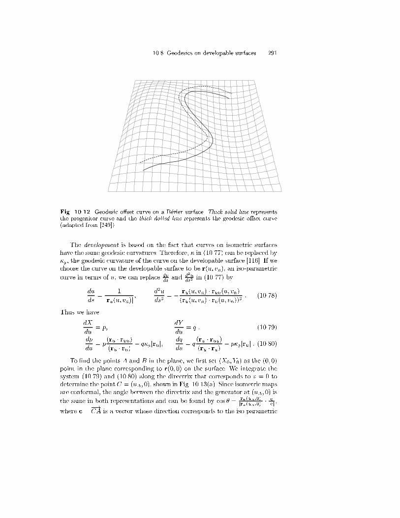
10.8 Geodesics on developable surfaces 291
Fig. 10.12. Geodesic o�set curve on a B�ezier surface. Thick solid line representsthe progenitor curve and the thick dotted line represents the geodesic o�set curve(adapted from [249])
The development is based on the fact that curves on isometric surfaceshave the same geodesic curvatures. Therefore, � in (10.77) can be replaced by�g , the geodesic curvature of the curve on the developable surface [116]. If wechoose the curve on the developable surface to be r(u; vn), an iso-parametric
curve in terms of u, we can replace duds and d2u
ds2 in (10.77) by
du
ds=
1
jru(u; vn)j ;d2u
ds2= � ru(u; vn) � ruu(u; vn)
(ru(u; vn) � ru(u; vn))2 : (10.78)
Thus we have
dX
du= p;
dY
du= q ; (10.79)
dp
du= p
(ru � ruu)(ru � ru) � q�gjruj;
dq
du= q
(ru � ruu)(ru � ru) + p�gjruj : (10.80)
To �nd the points A and B in the plane, we �rst set (X0; Y0) as the (0; 0)point in the plane corresponding to r(0; 0) on the surface. We integrate thesystem (10.79) and (10.80) along the directrix that corresponds to v = 0 todetermine the point C = (uA; 0), shown in Fig. 10.13(a). Since isometric mapsare conformal, the angle between the directrix and the generator at (uA; 0) is
the same in both representations and can be found by cos � = ru(uA;0)jru(uA;0)j � c
jcj ,
where c =�!CA is a vector whose direction corresponds to the iso-parametric

292 10. Geodesics
X
Y
θ
ωg(s)
A
B
C
(a) Surface developed onto plane (b) uv parametric space
u
v
θ
ωg(s)
(c) Geodesic on 3-D surface
R(0,0) C
A
B
xy
z
(d) 3-D surface with geodesic
Fig. 10.13. Geodesic on a degree (3,1) developable surface (adapted from [250])
line r(uA; v) which is a straight line on the surface. Therefore it is a geodesicand will be developed into the plane as a straight line. The distance is givenby jcj =p(xA � xC)2 + (yA � yC)2 + (zA � zC)2. The point A on the planeis found using C, jcj and �. The point B on the plane is found by following thesame procedure, and the points are connected as shown in Fig. 10.13(a). The
angle ! between c and b =��!AB is given by cos! = b�c
jbjjcj . The angles ! and
� are shown in Figs. 10.13(a) and (c). This angle ! is preserved between theiso-parametric line r(uA; v) and the geodesic curve g(s) on the developable
surface at point A. Thus we have cos! = rv�g0(s)jrv jjg0(s)j , where the tangent vector
to the geodesic is given by
g0(s) = rudu
ds+ rv
dv
ds: (10.81)
Multiplying (10.81) by rv yields
rv � g0(s) = ru � rv duds
+ rv � rv dvds
= cos(!)jrv jjg0(s)j ; (10.82)
which (since jg0(s)j = 1) can be reduced to

10.8 Geodesics on developable surfaces 293
dv
ds=
cos(!)pG� F
G
�du
ds
�; (10.83)
where F = ru � rv and G = rv � rv (coe�cients of the �rst fundamental form).From the �rst fundamental form,
g0(s) � g0(s) = E
�du
ds
�2
+ 2Fdu
ds
dv
ds+G
�dv
ds
�2
= 1 : (10.84)
Plugging (10.83) into (10.84) and solving for duds yields
du
ds= �
ssin2(!)G
EG� F 2; (10.85)
and thus (10.83) reduces to
dv
ds=
cos(!)pG� 1p
G
FpEG� F 2
sin(!) : (10.86)
Evaluating (10.85) and (10.86) at the initial point, we have all the initialconditions required to solve the IVP ((10.17) to (10.20)) for a geodesic. Thesolution to the IVP yields the uv parametric values for the geodesic that aregraphed in Fig. 10.13(b). The corresponding three-dimensional coordinatevalues are shown in Figs. 10.13(c) and (d). The geodesic runs from (uA; vA)= (0.1, 0.3) to (uB ; vB) = (0.9, 0.8).


11. O�set Curves and Surfaces
11.1 Introduction
11.1.1 Background and motivation
O�set curves/surfaces, also called parallel curves/surfaces, are de�ned as thelocus of the points which are at constant distant d along the normal from thegenerator curves/surfaces. A literature survey on o�set curves and surfaceswas carried out by Pham [312] and more recently by Maekawa [249]. O�setsare widely used in various applications, such as tool path generation for 2 12 -Dpocket machining [157, 153, 348], 3-D NC machining [116, 52, 214, 365] (seeFig. 11.1), in feature recognition through construction of skeletons or medialaxes of geometric models [297, 449] (see Fig. 11.2), de�nition of toleranceregions [93, 352, 296] (see Fig. 11.3), access space representations in robotics[236] (see Fig. 11.4), curved plate (shell) representation in solid modeling [300](see Fig. 11.5), rapid prototyping where materials are solidi�ed in successivetwo-dimensional layers [114] and brush stroke representation [197].
Because of the square root involved in the expression of the unit normalvector, o�set curves and surfaces are functionally more complex than theirprogenitors. If the progenitor is a rational B-spline, then its o�set is usu-ally not a rational B-spline, except for special cases including cyclide surfacepatches [331, 83, 403], Pythagorean hodograph curves and surfaces (see Sect.11.4) and simple solids [93]. Another di�culty arises when the progenitorhas a tangent discontinuity. Then its exterior and interior o�sets will becomediscontinuous or have self-intersections as illustrated in Fig. 11.6. Further-more o�sets may have cusps and self-intersections, even if the progenitor isregular (see Figs. 11.9, 11.25). Frequently in applications, discontinuity ino�sets must be �lled in and the loops arising from self-intersections must betrimmed o�. In the following three sections, we will brie y review some of theliterature on NC machining, medial axis transforms and tolerance regions.
11.1.2 NC machining
The purpose of milling is to remove material from a workpiece. The materialis removed in the form of small chips produced by the milling cutter which

296 11. O�set Curves and Surfaces
Center of Ball−EndMill
R
R
Design Surface
Tool Driving Plane
PickFeed
Tool PathOffset Surface
Machine Axis
(a) (b)
Fig. 11.1. NC machining: (a) 2 12-D pocket milling (adapted from [253]), (b) 3-D
milling (adapted from [222])
Fig. 11.2. Medial axis (adaptedfrom [139])
rotates at a high speed. A machine tool is characterized by the motions itcan perform. Such motions as changing the relative position of the tool andworkpiece consist of linear translations and rotations about di�erent axes.However, they do not include the rotation of the cutter or workpiece formaintaining cutting action. NC machines are classi�ed as follows [290, 157]:
2-D Milling : 2-D milling refers to the contouring capability of a machinetool limited to the xy-plane. By moving along the x and y axes simul-
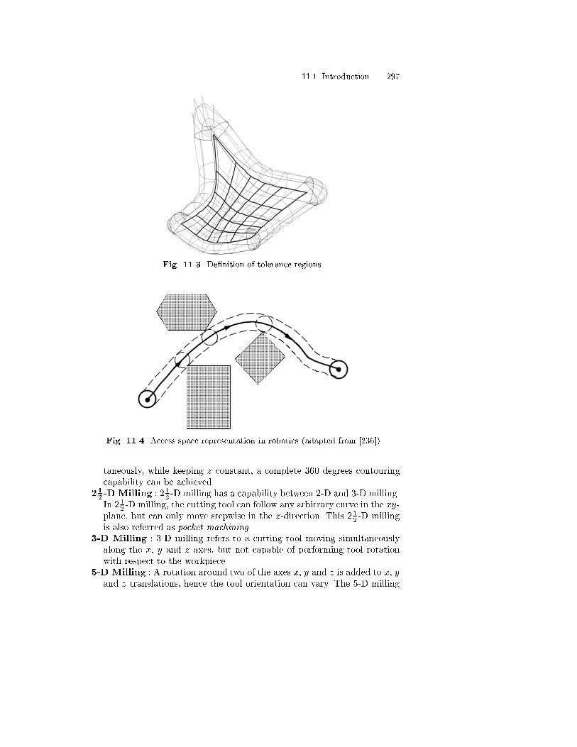
11.1 Introduction 297
Fig. 11.3. De�nition of tolerance regions.
BBBBBBBBBBBBBBBBBBBBBBBBBBBBBBBBBBB
BBBBBBBBBBBBBBBBBBBBBBBBBBBBBBBBBBBBBBBBBB
BBBBBBBBBBBBBBBBBB
Fig. 11.4. Access space representation in robotics (adapted from [236])
taneously, while keeping z constant, a complete 360 degrees contouringcapability can be achieved.
212-D Milling : 2 12 -D milling has a capability between 2-D and 3-D milling.In 2 12 -D milling, the cutting tool can follow any arbitrary curve in the xy-plane, but can only move stepwise in the z-direction. This 2 12 -D millingis also referred as pocket machining.
3-D Milling : 3-D milling refers to a cutting tool moving simultaneouslyalong the x, y and z axes, but not capable of performing tool rotationwith respect to the workpiece.
5-D Milling : A rotation around two of the axes x, y and z is added to x, yand z translations, hence the tool orientation can vary. The 5-D milling

298 11. O�set Curves and Surfaces
Fig. 11.5. Plate representation
(a) (b)
Fig. 11.6. O�sets to a tangent discontinuous curve (adapted from [253])
is suitable for large production runs, because the two additional rotationsreduce the required setups signi�cantly [286].
The success of NC milling highly depends on the availability of e�cient al-gorithms for de�ning tool paths. The books by Marciniak [261], and Choiand Jerard [59] provide theoretical and practical information on sculpturedsurface NC machining. The topic of optimal tool paths for NC machining ofsculptured surfaces is analyzed in [198].
The cutter motion for machining a part consists of roughing, semi-roughing and �nishing, and should be considered separately, as illustratedin Fig. 11.7 [231]. For each process, an appropriate tool size and tool pathneeds to be determined.

11.1 Introduction 299
Rough machining : It should be as simple as possible and preferablyconsist of a linear type motion only to minimize machining time. In otherwords, the cutter path should be as short as possible and the depth ofcut and feedrate should be as large as possible.
Semi-rough machining : After rough machining, the shoulders left on thepart should be removed.
Finishing machining : The cutter should follow the pro�le during theseoperations and the deviations of the cutter from the pro�le should alwaysbe maintained within a designated tolerance.
Part Surface Cutting Plane
Shoulders Left in Roughing
Flat−End Mill
@@@@@@@@@@@@@@@@@@@@@@@@@@@@@@@@@@@@@@@@@@@@@@@@@@@@@@@@@@@@@@@@@@@@@@@@@@@@@@@@@@@@@@@@@@@@@@@@@@@@@@@@@@@@@@@@@@@@@@@@@@@@@@@@@@@@@@@@@@@@@@@@@@@@@@@@@@@@@@@@@@@@@@@@@@@@@@@@@@@@
Part Surface
@@@@@@@@@@@@@@@@@@@@@@@@@@@@@@@@@@@@@@@@@@@@@@@@@@@@@@@@@@@@@@@@@@@@@@@@@@@@@@@@@@@@@@@@@@@@@@@@@@@@@@@@@@@@@@@@@@@@@@@@@@@@@@@@@@@@@@@
@@@@@@@@@@@@@@@@@@@@@@@@@@@@
Shoulders Left in Roughing
Ball−End Mill
FinishingAllowance
(a)
(b)
Moving Direction
Fig. 11.7. (a) Pocket machining with at-end mill in roughing, (b) semi-roughingwith large ball-end mill (adapted from [231])
More than 80% of all mechanical parts which are manufactured by millingmachines can be cut by NC pocket machining [157]. This is based on the factsthat most mechanical parts consist of faces parallel or normal to a single
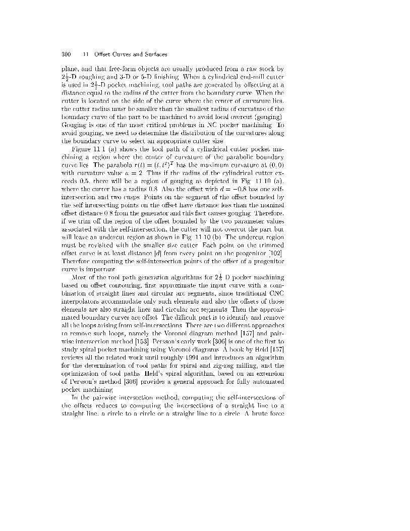
300 11. O�set Curves and Surfaces
plane, and that free-form objects are usually produced from a raw stock by2 12 -D roughing and 3-D or 5-D �nishing. When a cylindrical end-mill cutteris used in 2 12 -D pocket machining, tool paths are generated by o�setting at adistance equal to the radius of the cutter from the boundary curve. When thecutter is located on the side of the curve where the center of curvature lies,the cutter radius must be smaller than the smallest radius of curvature of theboundary curve of the part to be machined to avoid local overcut (gouging).Gouging is one of the most critical problems in NC pocket machining. Toavoid gouging, we need to determine the distribution of the curvatures alongthe boundary curve to select an appropriate cutter size.
Figure 11.1 (a) shows the tool path of a cylindrical cutter pocket ma-chining a region where the center of curvature of the parabolic boundarycurve lies. The parabola r(t) = (t; t2)T has the maximum curvature at (0; 0)with curvature value � = 2. Thus if the radius of the cylindrical cutter ex-ceeds 0:5, there will be a region of gouging as depicted in Fig. 11.10 (a),where the cutter has a radius 0:8. Also the o�set with d = �0:8 has one self-intersection and two cusps. Points on the segment of the o�set bounded bythe self-intersecting points on the o�set have distance less than the nominalo�set distance 0.8 from the generator and this fact causes gouging. Therefore,if we trim o� the region of the o�set bounded by the two parameter valuesassociated with the self-intersection, the cutter will not overcut the part butwill leave an undercut region as shown in Fig. 11.10 (b). The undercut regionmust be revisited with the smaller size cutter. Each point on the trimmedo�set curve is at least distance jdj from every point on the progenitor [102].Therefore computing the self-intersection points of the o�set of a progenitorcurve is important.
Most of the tool path generation algorithms for 2 12 -D pocket machiningbased on o�set contouring, �rst approximate the input curve with a com-bination of straight lines and circular arc segments, since traditional CNCinterpolators accommodate only such elements and also the o�sets of thoseelements are also straight lines and circular arc segments. Then the approxi-mated boundary curves are o�set. The di�cult part is to identify and removeall the loops arising from self-intersections. There are two di�erent approachesto remove such loops, namely the Voronoi diagram method [157] and pair-wise intersection method [153]. Persson's early work [306] is one of the �rst tostudy spiral pocket machining using Voronoi diagrams. A book by Held [157]reviews all the related work until roughly 1991 and introduces an algorithmfor the determination of tool paths for spiral and zig-zag milling, and theoptimization of tool paths. Held's spiral algorithm, based on an extensionof Persson's method [306] provides a general approach for fully automatedpocket machining.
In the pairwise intersection method, computing the self-intersections ofthe o�sets reduces to computing the intersections of a straight line to astraight line, a circle to a circle or a straight line to a circle. A brute force
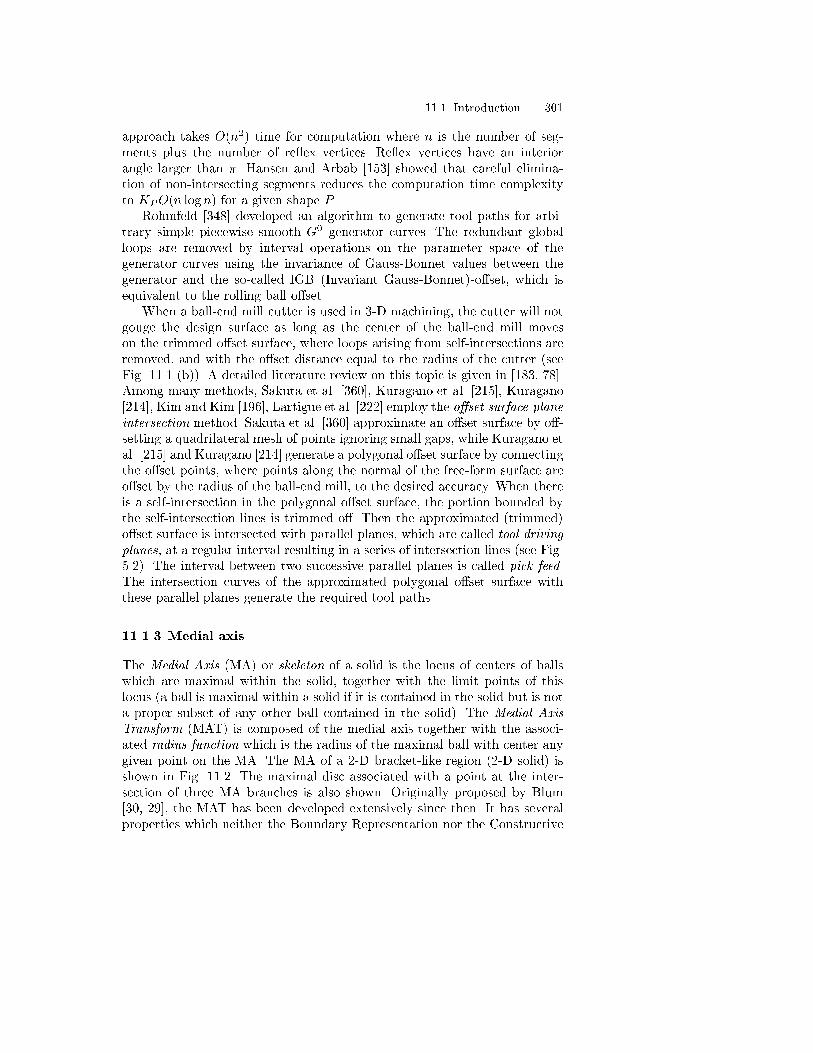
11.1 Introduction 301
approach takes O(n2) time for computation where n is the number of seg-ments plus the number of re ex vertices. Re ex vertices have an interiorangle larger than �. Hansen and Arbab [153] showed that careful elimina-tion of non-intersecting segments reduces the computation time complexityto KPO(n logn) for a given shape P .
Rohmfeld [348] developed an algorithm to generate tool paths for arbi-trary simple piecewise smooth G0 generator curves. The redundant globalloops are removed by interval operations on the parameter space of thegenerator curves using the invariance of Gauss-Bonnet values between thegenerator and the so-called IGB (Invariant Gauss-Bonnet)-o�set, which isequivalent to the rolling ball o�set.
When a ball-end mill cutter is used in 3-D machining, the cutter will notgouge the design surface as long as the center of the ball-end mill moveson the trimmed o�set surface, where loops arising from self-intersections areremoved, and with the o�set distance equal to the radius of the cutter (seeFig. 11.1 (b)). A detailed literature review on this topic is given in [183, 78].Among many methods, Sakuta et al. [360], Kuragano et al. [215], Kuragano[214], Kim and Kim [196], Lartigue et al. [222] employ the o�set surface-planeintersection method. Sakuta et al. [360] approximate an o�set surface by o�-setting a quadrilateral mesh of points ignoring small gaps, while Kuragano etal. [215] and Kuragano [214] generate a polygonal o�set surface by connectingthe o�set points, where points along the normal of the free-form surface areo�set by the radius of the ball-end mill, to the desired accuracy. When thereis a self-intersection in the polygonal o�set surface, the portion bounded bythe self-intersection lines is trimmed o�. Then the approximated (trimmed)o�set surface is intersected with parallel planes, which are called tool drivingplanes, at a regular interval resulting in a series of intersection lines (see Fig.5.2). The interval between two successive parallel planes is called pick feed.The intersection curves of the approximated polygonal o�set surface withthese parallel planes generate the required tool paths.
11.1.3 Medial axis
The Medial Axis (MA) or skeleton of a solid is the locus of centers of ballswhich are maximal within the solid, together with the limit points of thislocus (a ball is maximal within a solid if it is contained in the solid but is nota proper subset of any other ball contained in the solid). The Medial AxisTransform (MAT) is composed of the medial axis together with the associ-ated radius function which is the radius of the maximal ball with center anygiven point on the MA. The MA of a 2-D bracket-like region (2-D solid) isshown in Fig. 11.2. The maximal disc associated with a point at the inter-section of three MA branches is also shown. Originally proposed by Blum[30, 29], the MAT has been developed extensively since then. It has severalproperties which neither the Boundary Representation nor the Constructive

302 11. O�set Curves and Surfaces
Solid Geometry directly provide. First, because it elicits important symme-tries of an object, it facilitates the design and interrogation of symmetricalobjects [29]. Second, the MAT exhibits dimensional reduction [54, 449]; forexample, it transforms a 3-D solid into a connected set of points, curves, andsurfaces, along with an associated radius function described in more detail be-low. Third, once a solid is represented with the MAT, the skeleton and radiusfunction themselves may be manipulated, and the boundary will deform in anatural way, suggesting applications in computer animation [450]. Fourth, theskeleton may be used to facilitate the creation of coarse and �ne �nite elementmeshes of the region [139, 140, 141, 142, 297, 405, 12, 417, 337]. Fifth, theMAT determines constrictions and other global shape characteristics that areimportant in mesh generation, performance analysis, manufacturing simula-tion, and path planning [293, 297]. Sixth, the MAT can be used in documentencoding [43, 42] and other image processing applications [38]. Finally, theMAT may be useful in tolerance speci�cation [171].
The MA is closely related with equidistantial point sets, especially the wellknown Voronoi Diagram [334]. For a 2-D polygonal region or a 3-D polyhedralregion, the Voronoi Diagram is a superset of MA, while for objects withnonlinear boundary, the Voronoi Diagram may not be a superset of MA. Themajor di�erence is in that the MA is intrinsic to a solid, while the VoronoiDiagram depends on the speci�c decomposition of the boundary of the solid.
Algorithms for determining the MAT or related sets. The MAT wasintroduced and explored by Blum [30] and further explored by Blum [29]and Blum and Nagel [31] to describe biological shape. Soon after it wasintroduced, various algorithms for computing the MAT were developed forspecial planar regions. Montanari [271] developed an algorithm to computethe MAT of a multiply-connected polygonal region. His algorithm proceedsby identifying signi�cant branch points and propagating the boundary con-tour inward, while connecting the branch points with appropriate linear orparabolic segments. A more e�cient algorithm for computing the MAT of aconvex polygonal region in O(n logn) was presented by Preparata [333] alongwith an O(n2) algorithm for a non-convex polygonal region. Lee [228] devel-oped an O(n log n) algorithm for polygonal regions with non-convex corners.Srinivasan and Nackman [404] presented an O(nh + n logn) algorithm formultiply connected polygonal regions with h holes. Gursoy and Patrikalakis[140, 141, 142] developed an algorithm to compute the MAT of a multiplyconnected planar region bounded by line segments and circular arcs, andused this algorithm to generate �nite element meshes automatically and de-termine global shape characteristics. Guibas and Stol� [137] investigate therelationship between the Voronoi Diagram and the Delaunay Triangulation,and develop the quad-edge data structure to represent them. Sugihara [415]investigates the use of Voronoi Diagrams to approximate various types ofgeneralized Voronoi Diagrams. Rosenfeld [349] considers di�erent represen-tations of shapes based on an axis and a generation rule. Held's book [157]

11.1 Introduction 303
contains a comprehensive review of Voronoi Diagram algorithms, which heuses in the context of pocket machining. Another comprehensive review ofthe state of the art in Voronoi Diagram algorithms has been compiled byAurenhammer [14].
Other work has concentrated on discrete and approximate approaches todetermine the MAT or its related sets. Nackman [281] proposes a 3-D algo-rithm to use a polyhedral approximation of a smooth boundary and producea polyhedral approximation to the skeleton. The algorithm is an extension ofBookstein's line skeleton approach [36] to 3-D. It takes as input a polyhedralsurface made up of convex polygons and generates a connected graph of con-vex polygons approximating the MA of the original object; since the inputpolyhedron is assumed to be an approximation to a smooth curved object,the output is not the skeleton of the polyhedron itself but rather a collec-tion of polygons approximately tangent to the skeleton of the true object.Lavender et al. [225] use an octree-based approach to determine the VoronoiDiagram. Their algorithm works on set-theoretic solid models, composed ofunions, intersections, and di�erences of primitive regions represented by acollection of polynomial inequalities, and produces an octree (or quadtree intwo dimensions) which divides space into Voronoi regions at some speci�edresolution. Scott et al. [369] discuss a method for determining the SymmetricAxis (a superset of the MA) which is based on a combined wave/di�usionprocess in the plane. Their algorithm proceeds by assigning each boundarypixel a unit displacement above the plane and every other pixel a zero dis-placement, and then numerically propagating a wave from the boundary. Thewave is attenuated by a di�usion process to reduce numerical error, and localmaxima in the wave are declared to lie on the Symmetric Axis. Althoughuseful for binary images at low resolutions, the error may be large for higherresolutions. Memory and processing requirements for this method tend to bequite high as well.
Brandt, and Brandt and Algazi [41, 40, 39] �nd a continuous approxima-tion to the skeleton in both the planar and the 3-D case by �rst discretizingthe boundary. The boundary is sampled at a given sampling density, yieldinga set of discrete points which form a pixelized or voxelized approximation tothe boundary. The next step is to run an e�cient discrete-point Voronoi dia-gram on the set of points. Finally, portions of the skeleton which result fromthe e�ects of quantization are pruned away [39]. This approach attempts toclassify each of the vertices in the interior Voronoi diagram according to howmany foot points the vertex has. The number of footpoints is determinedby taking the associated maximal sphere at the vertex, increasing the radiusslightly, and intersecting the dilated sphere with the boundary. This intersec-tion partitions the surface of the sphere into areas which lie either inside oroutside the region. Each area lying outside the boundary is assumed to cor-respond to a footpoint; since the most commonly occurring type of skeleton

304 11. O�set Curves and Surfaces
point has two footpoints, only these points are kept, and the rest are prunedaway.
Chiang [54] takes a planar region bounded by piecewise C2 curves andperforms a cellular decomposition of the plane in a neighborhood of the re-gion. Each cell is assigned an approximate distance to the nearest point onthe boundary of the region using an algorithm due to Danielsson [70] whichcomputes the Euclidean distance transform. In order for us to explain theEuclidean distance transform, we consider a given binary image S (whereeach pixel (i; j) is assigned 0 or 1); we call �S the set of pixels with value 0.The distance map is de�ned as a scalar function on S
L(i; j) = min(d[(i; j); �S]) ; (11.1)
where d is a distance function. If d is the Euclidean distance between twopixels
de((i; j); (h; k)) =p(j � i)2 + (k � h)2 ; (11.2)
then the distance map is called the Euclidean distance map. This informationis later used to �nd a starting point for tracing axis branches in two dimen-sions and for recognizing when the tracing has passed the end of a branch.The tracing itself uses the distance information to determine on which bound-ary elements the footpoints of the current Medial Axis point lie. Once theseelements are known, a set of simultaneous equations describing the localstructure of the MA near the given point is formed. Using these equations todetermine the tangent to the MA at the given point, a short distance alongthe tangent is traversed, the point is re�ned with Newton iteration, and an-other tracing step is taken. At each step, the distance information is used todetermine whether or not the current branch has become inactive. If so, abranch point or an end point has been hit, and the tracing either proceedsalong another branch or stops. Although the tracing is not extended to threedimensions, Chiang [54] notes that the same Euclidean distance transform in3-D may be used to determine an approximation to the skeleton. One simpleway of using the distance transform in this way is to identify those pointswhich have locally maximal distance values after the distance transform iscarried out. Such points are clearly close to centers of maximal disks, and socan be considered to provide an approximation to the skeleton.
Sudhalkar et al. [414] introduce a set called the box skeleton which theyargue has the properties which make the MAT desirable as an alternate rep-resentation of shape. In particular, the box skeleton exhibits dimensionalreduction, homotopic equivalence and invertibility. However, their skeleton isde�ned using the L1 norm (the box norm) instead of the Euclidean normand thus may be quite di�erent from the Medial Axis. Their algorithm for de-termining the box skeleton operates on discrete objects made of unit squares(or cubes, in 3-D) and proceeds by thinning the object while maintaining ho-motopic equivalence to the original object. In order to perform the thinning,

11.1 Introduction 305
the object is transformed into a graph; in the planar case, the boundariesbetween adjacent pixels are considered to be edges of the graph, and the in-tersections of these edges are the vertices of the graph. The �rst thinning stepproceeds by replacing the graph by that portion of the dual graph which isinterior to the original (primal) graph. Since this procedure alone may resultin a disconnected skeleton, the boundary \shrink wraps" around the skeletonas it thins. Procedures based on these concepts are developed for both 2-Dand 3-D discrete objects.
Most of the 3-D algorithms in existence (such as the ones above) are fun-damentally discrete algorithms. To our knowledge, few continuous approacheshave been proposed, due largely to the computational complexity involved.One of the few such techniques is developed by Ho�mann [170], who proposeda method for assembling the skeleton of a CSG object. His method proceedsby determining points of closest approach between pairs of boundary ele-ments and checking these points to make sure they are in fact on the MedialAxis. (Each of these points are on the MA if and only if the distance to thepair of elements is less than or equal to the distances to the other boundaryelements.) The points are then sorted in order of increasing distance fromthe boundary, and then a local analysis around each point is performed, inan attempt to identify whether the point lies on a face, edge, or vertex ofthe Medial Axis. This determination is made by identifying all boundary el-ements which lie at the same minimum distance from the point and forminga set of simultaneous equations in n variables which describe the equidis-tantial set that the point belongs to. Based on the rank of the Jacobian ofthis set of equations, the point is predicted to lie on a face, edge, or vertexof the skeleton. Then neighboring faces and edges are traced out in order ofincreasing distance from the boundary. The method requires intersection ofequidistantial sets with one another in order to trim away portions whichdo not belong to the Medial Axis. Related papers by Dutta and Ho�mann[81, 82] consider the exact representation of the bisectors which appear asskeleton branches in the skeleton of CSG objects bounded by planes, naturalquadrics, and torii.
Reddy and Turkiyyah [340] propose an algorithm for determining theskeleton of a 3-D polyhedron based on a generalization of the Voronoi Dia-gram. They compute an abstract Delaunay Triangulation of the polyhedronand use the result to obtain the dual, the generalized Voronoi Diagram. TheDelaunay triangulation computed is a generalization of the usual Delaunaytriangulation, which connects isolated nodes together with line segments. Inthe generalization, the nodes represent parts of a polyhedron (speci�cally,either a face or a non-convex edge or a non-convex vertex of the polyhedron)and therefore the triangulation is an abstract graph. It still maintains dual-ity with the generalized Voronoi Diagram, and is easier to compute since theVoronoi Diagram may contain trimmed quadric surfaces. The skeleton of thepolyhedron is obtained by trimming away certain elements of the generalized

306 11. O�set Curves and Surfaces
Voronoi Diagram which are in the Voronoi Diagram but not the skeleton (forexample, the equidistantial point set between a face and a non-convex vertexbounding it). The algorithm can explicitly determine certain critical pointsof the skeleton, but does not contain highly accurate explicit representationsof the curves and surfaces making up the skeleton. Under the same approach,Turkiyyah et al. [427] developed an accelerated algorithm using Delaunaytriangulation with a local optimization scheme for the generation of accurateskeletons of 3D solid models. The accelerated algorithm has linear complexityin terms of the number of points used for skeleton approximation.
Sheehy et al. [384, 383] investigate the use of a domain Delaunay trian-gulation on a distribution of points on the boundary (in a manner similar toBrandt [39]) to attempt to determine the topological features of the MedialAxis of a 3-D solid. The steps of an algorithm to compute the Medial Axisfrom these features are outlined.
Sherbrooke et al. [392] developed an algorithm for determining the MAT ofa general polyhedral solid with simply connected faces and without cavities.In [393] and [390], that algorithm was re�ned, simpli�ed and extended towork for polyhedral solids of arbitrary genus without cavities, with nonconvexvertices and edges. The algorithm is based on a classi�cation scheme thatrelates di�erent pieces of the medial axis to one another even in the presenceof degenerate MA points. Vertices of the MA are connected to one anotherby tracing along adjacent edges, and �nally the faces of the axis are found bytraversing closed loops of vertices and edges. The completeness, complexityand stability of the algorithm were also analyzed.
Etzion and Rappoport [91] presented an algorithm for computing theVoronoi Diagram of a 3-D polyhedron based on subdivision of space. Thismethod enables local and partial computation of the Voronoi diagram. Byseparating the computation of the symbolic (Voronoi graph) and geometricparts of the diagram, the algorithm tends to be more robust. In addition, atracing algorithm for the MAT of a 3-D polyhedron is developed by Culveret al. [68] to improve accuracy using exact arithmetic and exact geometricrepresentations. In order to improve the e�ciency in searching MA elements,spatial decomposition and linear programming are utilized. Sheets in thismethods are in the form of quadrics. The method also includes a new al-gorithm for analysis of the topology of an algebraic plane curve and a fastnumerical method for implicit geometric computation.
Wolter and his associates [339, 450] compute medial curves on a surface,which is the locus of points being equidistant from two given curves on thesurface, utilizing the geodesic o�set function. Their method is also applicableto the plane curve case. Also Wolter and his associates [213] applied the abovemethod to compute a Voronoi diagram on a parametric surface instead of theusual Voronoi diagram in Euclidean space.
In addition to the work described above which discusses the determina-tion of the MAT, there has been additional work on the inverse problem of

11.1 Introduction 307
reconstructing the original solid from the Medial Axis and the radius function.Reconstruction of boundary surfaces from curves and surfaces of the MedialAxis in 3-D is discussed by Gelston and Dutta [125]. Vermeer [430] consid-ers the problem of boundary reconstruction from the MAT in 2-D and 3-D.Recently, Verroust and Lazarus [431] developed a method to extract skeletalcurves from a set of scattered points that are sampled from a surface using ageodesic graph and distance map with various levels of decomposition. Theskeletal curves extracted can be applied in surface reconstruction.
Work on the MAT and its applications has been somewhat limited by thedi�culty of developing an algorithm which is robust, accurate, and e�cient tocarry out the transformation especially for curved solids. Most recent workon the 3-D problem has tried to generate a discrete approximation to theactual MAT; while such algorithms may be well-suited for some meshingapplications, particularly if they involve some degree of user interaction, theyare less satisfactory for modeling since they do not capture the topologicalstructure of the shape accurately. However, because the skeleton is typicallypath connected, and because branch points on the skeleton may be expressed assolutions of a set of simultaneous nonlinear polynomial equations, we believethat a continuous approach to the problem is promising especially if combinedwith interval or even exact arithmetic methods, as for example in the recentwork by Culver et al. [68] for 3-D polyhedra.
Theoretical analysis of the MAT properties. There exists considerabletheoretical work on the mathematical properties of the MAT and other re-lated sets. Wolter [449] provides a thorough analysis of topological propertiesof the MAT in a very general context, and establishes the relationship be-tween the MA and related symmetry sets such as the cut locus. Principalresults of his paper include his proof of homotopic equivalence between anobject with a C2 boundary and its Medial Axis, the invertibility of the MAT(under conditions more general than piecewise C2 boundaries), and the C1
smoothness of the distance function on the complement of the cut locus. Fora 2-D solid with piecewise C2 boundaries, the medial axis is homotopicallyequivalent to the 2-D solid, which implies the connectedness of the medialaxis. Wolter [448, 446] also earlier analyzed the di�erentiability of the dis-tance function.
Farouki and Johnstone [99, 100] have studied bisector problems between aplanar curve and a point on its plane, and between two co-planar curves. Theyintroduce a natural method for tracing the bisector between two curves byusing the exact representation of the bisectors of the �rst curve and successivepoints on the second curve.
Chiang [54] and Brandt [38, 39] studied many of the mathematical proper-ties of the MAT, primarily for the domain of 2-D regions. Chiang [54] providesa proof that for two-dimensional regions with piecewise C2 boundaries, theMA is connected, the MAT is invertible, and, provided the 2-D solid is home-omorphic to the closed unit disk, the maximal disc of a given MA point (not

308 11. O�set Curves and Surfaces
an end point of a MA arc) divides the MA and the solid into two disjointtrees and two disjoint 2-D solids, respectively (which provides justi�cationfor divide-and-conquer approaches). Brandt [38, 39] computes �rst order andsecond order di�erential properties of the planar skeleton, and explores thedetermination of the skeleton under di�erent metrics (which may be usefulfor determining the skeleton of binary images). He also explores the notion ofskeleton point classi�cation [39], classifying skeleton points according to thenumber of footpoints.
The three-dimensional problem is studied in some detail by Nackman[281] and Nackman and Pizer [282], who also derive relationships betweencurvatures of the boundary, the skeleton, and the associated radius func-tion. Curvature relationships in the planar case are considered by Blum [29].Anoshkina et al. [9, 8] consider properties of the Medial Axis in the contextof an investigation of singularities of the distance function to the boundingsurface.
Sherbrooke et al. [394, 390] further developed the theory of the MATof 3-D objects. They established the relationships between the curvature ofthe boundary and the position of the medial axis and also set up a defor-mation retract between each object and its medial axis for n-dimensionalsubmanifolds of Rn with boundaries which are piecewise C2 and completelyG1. They demonstrated that if the object is path connected, then so is themedial axis. Speci�cally, they proved that path connected polyhedral solidswithout cavities have path connected medial axes.
Stifter [406, 407] considers the Voronoi Diagram of any subset of 3-Dspace characterized by certain axioms and analyzes various properties of thesubset with applications to robotics.
11.1.4 Tolerance region
A tolerance region of a solid is constructed according to the ball-o�set oper-ator model as in Rossignac [350]. Farouki [93] studied the problem of �ndingexact o�sets on the exterior of simple solids. He handled the tangent discon-tinuities at the edge and vertices by using the rolling ball o�set de�nition.The class of solids studied are closed convex solids like solids of revolutionand extrusion.
Patrikalakis and Bardis [296] construct a tolerance region of a quadrilat-eral design surface patch which is bounded by ten surfaces as illustrated inFig. 11.3. For the shapes of interest in practical applications and the strict tol-erance requirements under consideration, they assumed that there will be noself-intersections in the ten bounding surfaces. These ten surfaces are: 1) fourpipe or canal surfaces (see Sect. 11.6), the o�sets to the edges of the designsurface; 2) two o�set surfaces, one along the normal and one in the oppositedirection to that of the normal to the design surface; 3) four spherical surfacepatches, the o�sets of the corners of the design surface. They approximatedthe pipe surfaces with rational B-splines and the normal o�sets by integral

11.2 Planar o�set curves 309
B-splines and expressed the spherical segments exactly by rational B-splinesurface patches. It is interesting to note that the design surface is the medialaxis of the tolerance region.
11.2 Planar o�set curves
11.2.1 Di�erential geometry
C
P
r(t)
n t
x
y
ez
Fig. 11.8. De�nitions of unit tangent and normal vectors (adapted from [253])
In this entire chapter we employ the convention (b) (see Fig. 3.7 (b) andTable 3.2) such that the curvature � of a curve at point P is positive whenthe center of curvature C is on the opposite direction of the unit normalvector n as illustrated in Fig. 11.8. Following this convention, the Frenet-Serret formulae for a planar curve r = r(t), t1 � t � t2 with arbitrary speed(2.57) reduce to
_t = �v�n; _n = v�t ; (11.3)
where v = j _r(t)j is the parametric speed. The second equation of (11.3) canbe rewritten as follows:
_n = � _r : (11.4)
A planar o�set curve r(t) with signed o�set distance d to the progenitorplanar curve r(t) is de�ned by

310 11. O�set Curves and Surfaces
r(t) = r(t) + dn(t) : (11.5)
The unit tangent and normal vectors and the curvature of the o�set curveare given by [102]
t =_r
j _rj =1 + �d
j1 + �djt ; (11.6)
n = t� ez = 1 + �d
j1 + �djn ; (11.7)
� =�
j1 + �dj ; (11.8)
where (11.3) (11.4) are used for the derivation.
11.2.2 Classi�cation of singularities
There are two types of singularities on the o�set curves of a regular progenitorcurve, irregular points and self-intersections. Irregular points include isolatedpoints and cusps. A point P on a curve C is called an isolated point of C ifthere is no other point of C in some neighborhood of P . This point occurswhen the progenitor curve with radius R is a circle and the o�set is d = �R.A cusp is an irregular point on the o�set curve where the tangent vectorvanishes. Cusps at t = tc can be further subdivided into ordinary cusps when_�(tc) 6= 0 and extraordinary points when _�(tc) = 0 and ��(tc) 6= 0 [102]. Anisolated point and a cusp occur when j _r(t)j = 0, which using (11.6) reducesto
�(t) = �1d: (11.9)
Note that (1 + �d)=j1+ �dj in (11.6) and (11.7) changes abruptly from -1 to1 when the parameter t passes through t = tc at an ordinary cusp, while atextraordinary points (1+�d)=j1+�dj does not change its value (see Fig. 11.9(b)).
O�set curve/surface may self-intersect locally when the absolute valueof the o�set distance exceeds the minimum radius of curvature in the con-cave regions (see Fig. 11.10 (a)). Also the o�set curve/surface may self-intersect globally when the distance between two distinct points on thecurve/surface reaches a local minimum (i.e. the presence of a constrictionof the curve/surface as illustrated in Fig. 11.11). These local and globalself-intersections can be visualized as machining a part using a cylindri-cal/spherical cutter whose radius is too large for 2 12 -D/3-D milling. It isan essential task for many practical applications to detect all componentsof the self-intersection points/curves correctly and generate the trimmed o�-set curve/surface. If the cutter follows the trimmed o�set, there will be no

11.2 Planar o�set curves 311
(a) (b)
Fig. 11.9. (a) O�sets to a parabola r = (t; t2)T , �2 � t � 2 (thick solid line)with o�sets d=-0.3, -0.5, -0.8 (adapted from [94]), (b) at d=-0.3, -0.5 the tangentand normal vectors of the o�set have the same sense as the progenitor, while atd = �0:8 they ip directions
overcut or gouging, however we are left with undercut regions which must bemilled with a smaller size cutter (see Fig. 11.10 (b)).
Self-intersections of o�set curves include nodes and tacnodes. A node Pis a point of curve C where two arcs of C pass through P and the arcs havedi�erent tangents. A tacnode is a special case of a node whose two tangentscoincide, as illustrated in Fig. 11.11. Self-intersections of an o�set curve canbe obtained by seeking pairs of distinct parameter values � 6= t such that
r(�) + dn(�) = r(t) + dn(t) : (11.10)
Example 11.2.1. (see Figs. 11.9 and 11.10)Given a parabola r = (t; t2)T , �2 � t � 2, the unit tangent and normalvectors are given by
t =dr
ds=dr
dt
dt
ds=
(1; 2t)Tp1 + 4t2
; n = t� ez = (2t;�1)Tp1 + 4t2
:
The curvature and its �rst and second derivatives are given by
�(t) =(_r� �r) � ezj _rj3 =
2
(1 + 4t2)32
> 0 ;
_�(t) =�24t(1 + 4t2)
12
(1 + 4t2)3; ��(t) =
24(16t2 � 1)
(1 + 4t2)72
:

312 11. O�set Curves and Surfaces
(a) (b)
Fig. 11.10. Self-intersection of the o�set curve of a parabola (adapted from [253]):(a) o�sets to the parabola r(t) = (t; t2)T with d = �0:8 and cutter path withgouging, (b) trimmed o�sets to the parabola r(t) = (t; t2)T with d = �0:8 andcutter path with undercut
Thus a stationary point of curvature occurs at t = 0. Since ��(0) = �24 < 0,�(0) is a maximum with a curvature value �(0) = 2. It is evident that theo�set distance d has to be negative to have a cusp, since �(t) is always positivefor any t. Now let us solve �(t) = �1=d for t which yields
t = �p
3p4d2 � 1
2:
We can easily see that if d > � 12 , there is no real root. This means that there
is no singularity as long as the magnitude of the o�set distance is smallerthan 1
2 . If d = � 12 , there exists a double root t = 0, while if d < �1=2 there
exist two symmetric values of t. When d = � 12 , at t = 0, we have _�(0) = 0,
��(0) 6= 0, therefore t = 0 is an extraordinary point, while when d < � 12 ,
_�(�tc) 6= 0, so at points t = �tc there are ordinary cusps on the o�set curve.The o�set to the parabola r = (t; t2)T is given by
r = (t; t2)T + d(2t;�1)Tp1 + 4t2
:
Therefore the equations for self-intersection of o�set curve to the parabola inx and y components become
� +2d�p1 + 4�2
= t+2dtp1 + 4t2
;
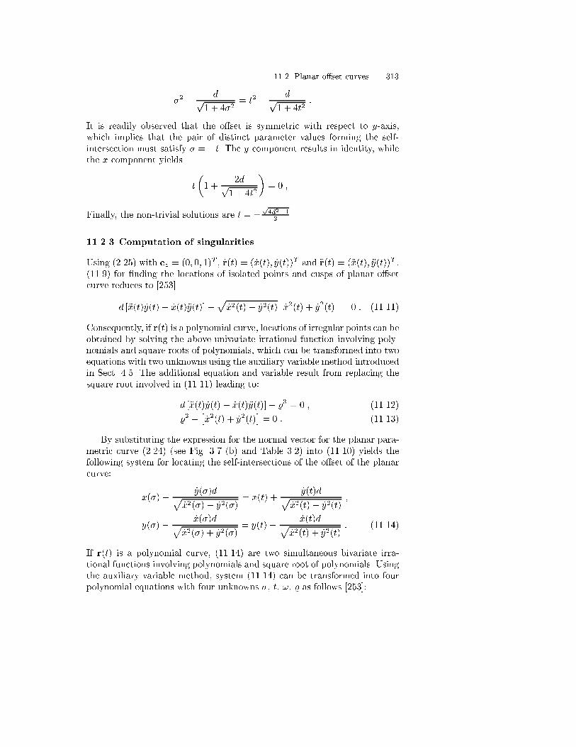
11.2 Planar o�set curves 313
�2 � dp1 + 4�2
= t2 � dp1 + 4t2
:
It is readily observed that the o�set is symmetric with respect to y-axis,which implies that the pair of distinct parameter values forming the self-intersection must satisfy � = �t. The y component results in identity, whilethe x component yields
t
�1 +
2dp1 + 4t2
�= 0 ;
Finally, the non-trivial solutions are t = �p4d2�12 .
11.2.3 Computation of singularities
Using (2.25) with ez = (0; 0; 1)T , _r(t) = ( _x(t); _y(t))T and �r(t) = (�x(t); �y(t))T ,(11.9) for �nding the locations of isolated points and cusps of planar o�setcurve reduces to [253]
d [�x(t) _y(t)� _x(t)�y(t)]�p
_x2(t) + _y2(t)�_x2(t) + _y2(t)
�= 0 : (11.11)
Consequently, if r(t) is a polynomial curve, locations of irregular points can beobtained by solving the above univariate irrational function involving poly-nomials and square roots of polynomials, which can be transformed into twoequations with two unknowns using the auxiliary variable method introducedin Sect. 4.5. The additional equation and variable result from replacing thesquare root involved in (11.11) leading to:
d [�x(t) _y(t)� _x(t)�y(t)]� %3 = 0 ; (11.12)
%2 � � _x2(t) + _y2(t)�= 0 : (11.13)
By substituting the expression for the normal vector for the planar para-metric curve (2.24) (see Fig. 3.7 (b) and Table 3.2) into (11.10) yields thefollowing system for locating the self-intersections of the o�set of the planarcurve:
x(�) +_y(�)dp
_x2(�) + _y2(�)= x(t) +
_y(t)dp_x2(t) + _y2(t)
;
y(�)� _x(�)dp_x2(�) + _y2(�)
= y(t)� _x(t)dp_x2(t) + _y2(t)
: (11.14)
If r(t) is a polynomial curve, (11.14) are two simultaneous bivariate irra-tional functions involving polynomials and square root of polynomials. Usingthe auxiliary variable method, system (11.14) can be transformed into fourpolynomial equations with four unknowns �, t, !, % as follows [253]:

314 11. O�set Curves and Surfaces
!% [x(�) � x(t)] + d [% _y(�) � ! _y(t)] = 0 ;
!% [y(�)� y(t)] + d [�% _x(�) + ! _x(t)] = 0 ;
!2 � � _x2(�) + _y2(�)�= 0 ;
%2 � � _x2(t) + _y2(t)�= 0 : (11.15)
The trivial solution � = t can be avoided by factoring out � � t from theabove equations. It is apparent that the two additional equations obtainedthrough the auxiliary variables do not contain the factor � � t. However,the original two equations, where the square roots of polynomials have beenreplaced by the auxiliary variables, possess the factor � � t as can beenseen after some algebraic manipulations [253]. Once the division operationsare completed, we obtain a system of four polynomial equations with fourunknowns without the trivial solution � = t.
Similarly to (11.14), intersections of the normal o�sets at distance d oftwo distinct planar curves rA(�) and rB(t) can be computed by solving thefollowing system:
xA(�) +_yA(�)dp
( _xA)2(�) + ( _yA)2(�)= xB(t) +
_yB(t)dp( _xB)2(t) + ( _yB)2(t)
;
yA(�) � _xA(�)dp( _xA)2(�) + ( _yA)2(�)
= yB(t)� _xB(t)dp( _xB)2(t) + ( _yB)2(t)
:
(11.16)
Note that for (11.14) we need to �nd a method to eliminate the trivial solution� = t, while for (11.16) � = t can be a solution. When the input curve is aB-spline curve, we can always split it into B�ezier (polynomial) segments by aknot insertion algorithm [34, 63]. In such cases not only the self-intersectionin the o�set of each split polynomial segment but also the intersections amongthe o�sets of di�erent split segments must be checked.
A system of nonlinear polynomial equations can be robustly and e�-ciently solved by the subdivision-based Interval Projected Polyhedron algo-rithm [253, 179], which was introduced in Chap. 4. A remarkable feature ofthis algorithm when applied to the system (11.15) is that both local andglobal self-intersections can be found by the same algorithm without anyinitial approximations (see Figs. 11.10, 11.11, 11.12).
11.2.4 Approximations
In general, an o�set curve is functionally more complex than its progenitorcurve because of the square root involved in the expression of the unit normalvector. If the progenitor is a NURBS curve, then its o�set is usually not aNURBS curve, except for some special cases such as straight lines and circlesetc. L�u [237] has shown that the o�set of a parabola is a rational curve. How-ever, this result has not been generalized to higher order curves. Farouki and

11.2 Planar o�set curves 315
(a) (b)
Fig. 11.11. Global self-intersections of o�sets: (a) degree six B�ezier curve andits o�set with d = �0:05, (b) o�set curve self-intersects forming a tacnode withd ' �0:03141 (adapted from [253])
Ne� [101] have shown that the two-sided o�sets of planar rational polyno-mial curves are high-degree implicit algebraic curves of potentially complexshape. These equations cannot typically be separated into two equations de-scribing positive and negative o�sets individually. The degree of this implicito�set curve is no = 4n � 2 � 2m, where n is the degree of polynomial gen-erator curve r = (x(t); y(t))T and m is the degree of �(t) = GCD( _x(t); _y(t))where GCD denotes the greatest common divisor. For example the degree ofthe two-sided o�set curve of a parabola r(t) = (t; t2)T is 6 and of a generalpolynomial cubic curve is 10 with �(t) a constant.
Because of the wide application of o�set curves and the di�culty in di-rectly incorporating such entities in geometric modeling systems, due to theirpotential analytic and algebraic complexity, a number of researchers have de-veloped approximation algorithms for these types of geometries in terms ofpiecewise polynomial or rational polynomial functions. A literature surveyon approximation of planar o�set curves is compiled in [312, 249]. A paperby Elber et al. [88] presented qualitative as well as quantitative comparisonsfor several plane o�set curve approximation methods, namely the controlpolygon-based methods by Cobb [62], Tiller and Hanson [420], Coquillart[65], and Elber and Cohen [86], the interpolation methods by Klass [202],and Pham [311], the least square methods by Hoschek [174], the nonlinearoptimization technique by Hoschek and Wissel [176], and the circle approxi-mation method by Lee et al. [229]. They counted the number of control points

316 11. O�set Curves and Surfaces
(a) (b)
Fig. 11.12. (a) Trimmed o�set of degree six B�ezier curve with d = �0:05, (b) toolpath along the trimmed o�set (adapted from [253])
of the approximated o�set as a measure for e�ciency, while the approxima-tion error was within a prescribed tolerance. They found in general that theleast square methods perform very well. However, when the progenitor curveis quadratic they showed that the simple method due to Tiller and Hanson[420], which translates each edge of the control polygon into the edge normaldirection by an o�set distance, outperforms the other methods. Therefore asan example we summarize the algorithm by Tiller and Hanson [420] with anillustration in Fig. 11.13:
1. Let C be a rational B-spline progenitor curve with control vertices p(1)in homogeneous representation and knot vector T(1). Set i = 1.
2. O�set each leg of the control polygon by d.3. Intersect consecutive legs of polygon to �nd new vertices p(i). Then the
approximated o�set C is de�ned by p(i) and T(i).4. Check deviation of the approximate o�set from the true o�set.5. If the deviation is larger than the given tolerance subdivide p(i) and T(i)
to obtain p(i+1) and T(i+1). Then set i i + 1 and go back to step 2.Stop if the deviation is smaller than the given tolerance.
Sederberg and Buehler [374] approximate an o�set of a B�ezier curve usingHermite interpolation of any even degree not less than the degree of the initial

11.2 Planar o�set curves 317
dd
d
Approximated Offset Curve
Progenitor Curve
Fig. 11.13. O�set curve approximation
B�ezier curve. The representation of the o�set is a special interval B�eziercurve of even degree with only the middle control point as a rectangularinterval. The size of the rectangular interval indicates the tightness of theapproximation.
Most of the existing o�set approximation schemes generate the approxi-mate o�set curve in terms of B�ezier /B-spline format in an iterative mannerbased on a subdivision technique to improve the accuracy of the o�set curve.If local and global self-intersections exist, they must be eliminated after theapproximation. Elber and Cohen [85] identify the local loops by using thefact that a pair of cusps always exist within the local self-intersection loop ofthe o�set curve. The tangent vector of the o�set t(t) ips its direction at thecusps, and thus !(t) = t(t) � t(t), where t(t) is the tangent vector of the inputcurve, becomes negative at the regions bounded by the cusps. Consequently,the local loops can be identi�ed by �nding the zero set of !(t). Once a localloop is identi�ed the curve is split into three parts, the region before the�rst cusp, the region between the cusps and the region after the second cusp.The o�set of the curve before the �rst cusp and the o�set of the curve afterthe second cusp are intersected to �nd the self-intersection point. The regionbounded by the parameters corresponding to the self-intersection point aretrimmed o�.
Lee et al. [229] eliminate the local and global self-intersections by approx-imating the input curve by discrete points and the connecting polygon. Thenthe o�set curve is generated by o�setting these discrete points. The local re-dundant polygon edges can be detected by checking the dot product betweenthe line segment and its corresponding o�set line segment. If the dot productis negative, the o�set segment is eliminated. The global self-intersections aredetected by a plane sweep algorithm among the o�set line segments. Oncea valid boundary topology on the o�set polygon is computed, the valid pa-rameter intervals of the input curve are extracted. The intersection pointsof polygonal approximations may not provide accurate parameter values forthe intersection points of the o�set curve and hence they need to be re�nedusing, for example Newton's method.

318 11. O�set Curves and Surfaces
The method introduced by Kimmel and Bruckstein [200] generates o�setsvia wavefront propagation methods in uid dynamics. The algorithm workson a square grid with a resolution chosen according to the desired accuracy.Finally the contour lines (o�sets) are generated based on grid values. Gurbuzand Zeid [138] employ a di�erent approach to avoid self-intersections. Insteadof o�setting analytically, the o�setting process is carried out by �lling theclosed balls of radius d for each point on the object. The union of the closedballs is subtracted from the object to construct the o�set. An o�set of apoint in space is considered as a sphere. They simpli�ed the implementationby assuming that the shape of a point is a cube and its o�set is also a cube.First the object to be o�set and its enclosing space are divided into smallcubic cells. Therefore the accuracy is governed by the size of the cell. The cellsthat are on the object are referred to as boundary cells. The boundary cellsseparate the original set of cells into two subspaces, in and out of the object.O�set operation is carried out for each boundary cell. Chiang et al. [55]also compute o�sets without self-intersections using a technique developed inimage processing. First the domain is discretized into a two-dimensional gridand the progenitor curve is assigned to the nearest grid point. For each gridpoint, the distance to the discretized curve is evaluated. By extracting thegrid points whose distances are equal to the o�set distance, an o�set withoutself-intersection can be constructed. This approach also obviously involves atrade-o� between accuracy achieved and memory required.
11.3 O�set surfaces
11.3.1 Di�erential geometry
A parametric o�set surface r(u; v) is a continuum of all points at a constantdistance d along normal to another parametric surface r(u; v) and de�ned as
r(u; v) = r(u; v) + dN(u; v) ; (11.17)
where d may be a positive or negative real number and N is the unit normalvector of r(u; v) (see (3.3)). As we mentioned at the beginning of this chapterwe employ the convention that the normal curvature is positive if its asso-ciated center of curvature is opposite to the direction of the surface normal(see Fig. 3.7 (b) and Table 3.2).
If N(u; v) is the unit normal vector of r(u; v), then the relation between
N and N is given by [443]
SN = (1 + d�max)(1 + d�min)SN ; (11.18)
where S = jru � rv j and S = jru � rvj or expanding the right hand side of(11.18) and using the de�nitions of Gaussian curvature K (3.61) and meancurvature H (3.62), (11.18) can be rewritten as follows:

11.3 O�set surfaces 319
SN = S(1 + 2Hd+Kd2)N : (11.19)
If we take the norm of (11.18), we obtain
S = Sj(1 + d�max)(1 + d�min)j ; (11.20)
and substituting S into (11.18) yields
N =(1 + d�max)(1 + d�min)
j(1 + d�max)(1 + d�min)jN : (11.21)
If we denote by
e =1+ 2Hd+Kd2
j1 + 2Hd+Kd2j =(1 + d�max)(1 + d�min)
j(1 + d�max)(1 + d�min)j = �1 ; (11.22)
then (11.21) gives
N = eN : (11.23)
From this relation we can see thatN and N are collinear but may be directedin opposite directions, if d�max + 1 and d�min + 1 have opposite signs. Thisoccurs when the o�set is taken towards the concave region of the progenitorsurface. O�setting towards the concave region of a surface is equivalent totaking the o�set d > 0 where �min < 0 and d < 0 where �max > 0, providedthe above sign convention is used. In machining, the cutter radius must notexceed the smallest concave principal radius of curvature of the surface toavoid gouging [116].
Principal curvatures of the o�set surface corresponding to �max and �min
of the progenitor surface can be easily obtained by adding the signed o�setdistance to the signed radius of principal curvature of the progenitor surfaceand inverting it. Taking into account the direction in which the normal vectorpoints, we have
�a =e�max
1 + d�max; (11.24)
�b =e�min
1 + d�min: (11.25)
Gaussian and mean curvatures of the o�set surface are readily computedby
K = �a�b =K
1 + 2Hd+Kd2; (11.26)
H =�a + �b
2=
H +Kd
j1 + 2Hd+Kd2j : (11.27)
Given the o�set distance d, the critical curvature is de�ned as �crit =�1=d and three categories arise [94]:
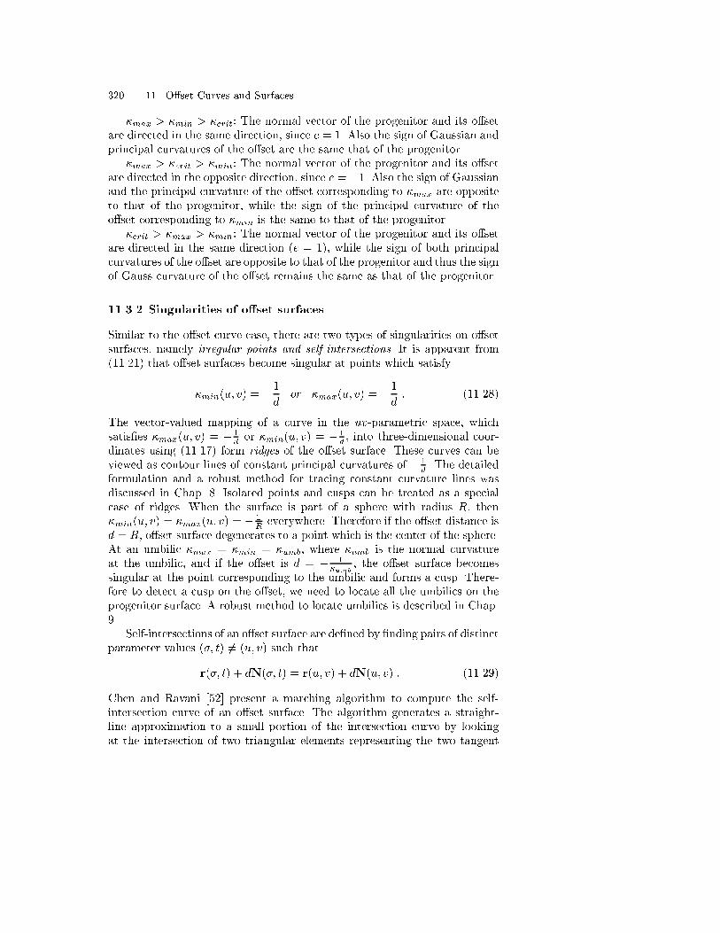
320 11. O�set Curves and Surfaces
�max > �min > �crit: The normal vector of the progenitor and its o�setare directed in the same direction, since e = 1. Also the sign of Gaussian andprincipal curvatures of the o�set are the same that of the progenitor.
�max > �crit > �min: The normal vector of the progenitor and its o�setare directed in the opposite direction, since e = �1. Also the sign of Gaussianand the principal curvature of the o�set corresponding to �max are oppositeto that of the progenitor, while the sign of the principal curvature of theo�set corresponding to �min is the same to that of the progenitor.
�crit > �max > �min: The normal vector of the progenitor and its o�setare directed in the same direction (e = 1), while the sign of both principalcurvatures of the o�set are opposite to that of the progenitor and thus the signof Gauss curvature of the o�set remains the same as that of the progenitor.
11.3.2 Singularities of o�set surfaces
Similar to the o�set curve case, there are two types of singularities on o�setsurfaces, namely irregular points and self-intersections. It is apparent from(11.21) that o�set surfaces become singular at points which satisfy
�min(u; v) = �1d
or �max(u; v) = �1d: (11.28)
The vector-valued mapping of a curve in the uv-parametric space, whichsatis�es �max(u; v) = � 1
d or �min(u; v) = � 1d , into three-dimensional coor-
dinates using (11.17) form ridges of the o�set surface. These curves can beviewed as contour lines of constant principal curvatures of � 1
d . The detailedformulation and a robust method for tracing constant curvature lines wasdiscussed in Chap. 8. Isolated points and cusps can be treated as a specialcase of ridges. When the surface is part of a sphere with radius R, then�min(u; v) = �max(u; v) = � 1
R everywhere. Therefore if the o�set distance isd = R, o�set surface degenerates to a point which is the center of the sphere.At an umbilic �max = �min = �umb, where �umb is the normal curvatureat the umbilic, and if the o�set is d = � 1
�umb, the o�set surface becomes
singular at the point corresponding to the umbilic and forms a cusp. There-fore to detect a cusp on the o�set, we need to locate all the umbilics on theprogenitor surface. A robust method to locate umbilics is described in Chap.9.
Self-intersections of an o�set surface are de�ned by �nding pairs of distinctparameter values (�; t) 6= (u; v) such that
r(�; t) + dN(�; t) = r(u; v) + dN(u; v) : (11.29)
Chen and Ravani [52] present a marching algorithm to compute the self-intersection curve of an o�set surface. The algorithm generates a straight-line approximation to a small portion of the intersection curve by lookingat the intersection of two triangular elements representing the two tangent

11.3 O�set surfaces 321
planes to the self-intersecting surfaces. The starting line segment is obtainedby searching only the bounding curves of the patch. Aomura and Uehara [11]also developed a marching method to compute the self-intersection curves onthe o�set surface of a uniform bicubic B-spline surface patch. The startingpoints for marching are obtained by the Powell-Zangwill method based on adense grid of points. Then the self-intersection curves are traced by integrat-ing a system of ordinary di�erential equations using the Runge-Kutta-Gillmethod. Visualization of self-intersecting o�sets of B�ezier patches by meansof ray tracing was studied in [429]. Self-intersection of o�sets of regular B�eziersurface patches due to local di�erential geometry and global distance functionproperties is investigated by Maekawa et al. [252]. The problem of comput-ing starting points for tracing self-intersection curves of o�sets is formulatedin terms of a system of nonlinear polynomial equations and solved robustlyby the Interval Projected Polyhedron algorithm. Trivial solutions are ex-cluded by evaluating the normal bounding pyramids of the surface subpatchesmapped from the parameter boxes computed by the polynomial solver witha coarse tolerance (see Sect. 11.3.5). Since it is an essential task for manypractical applications to detect all components of the self-intersection curvesand to trace them correctly for generating the trimmed o�set, we will dis-cuss this topic in greater detail in the following three sections. In Sect. 11.3.3we discuss the self-intersection of o�sets of implicit quadratic surfaces, whilein Sect. 11.3.4 we discuss the self-intersection of o�sets of explicit quadraticsurfaces. In Sect. 11.3.5 we introduce a method to �nd the self-intersectionsof o�sets of more general polynomial parametric surface patches.
11.3.3 Self-intersection of o�sets of implicit quadratic surfaces
The second order algebraic surfaces (i.e. quadric surfaces) are widely usedin mechanical design. Especially the natural quadrics, i.e. sphere, circularcone and circular cylinder result from machining operations such as rolling,turning, �lleting, drilling and milling [149]. The o�sets of the natural quadricsare also natural quadrics. Implicit quadrics such as ellipsoids, elliptic conesand elliptic cylinders are commonly found in die cavities and punches and aremanufactured by NC machining [60]. Although Salmon [361] discussed theo�sets of quadrics more than a century ago, this was not widely known in theCAGD literature until recently. Maekawa [248] showed that self-intersectioncurves of o�sets of all the implicit quadratic surfaces are planar implicit conicsand their corresponding curve on the progenitor surface can be expressed asthe intersection curve between an ellipsoid, whose semi-axes are proportionalto the o�set distance, and the implicit quadratic surfaces themselves.
The equations of implicit quadrics including ellipsoids, hyperboloids ofone and two sheets, elliptic cones, elliptic cylinders and hyperbolic cylinderscan be expressed in a standard form (3.74). In the sequel we assume a � b � cwithout loss of generality.

322 11. O�set Curves and Surfaces
The components x, y, z of the position vector r of the o�set of implicitsurface f(x; y; z) = 0 can be expressed as
x(x; y; z) = x+fx(x; y; z)
jrf(x; y; z)jd ; (11.30)
y(x; y; z) = y +fy(x; y; z)
jrf(x; y; z)jd ; (11.31)
z(x; y; z) = z +fz(x; y; z)
jrf(x; y; z)jd ; (11.32)
where (x; y; z) satisfy f(x; y; z) = 0 and fx, fy, fz are the x, y z componentsof rf(x; y; z). Note that jrf(x; y; z)j is zero at the apex of a cone and inthis case the normal vector is not de�ned. Substituting (3.74) into (11.30),(11.31), (11.32) yields
x(x; y; z) = x+�xd
a2q�2 x
2
a4 + �2 y2
b4 + �2 z2
c4
; (11.33)
y(x; y; z) = y +�yd
b2q�2 x
2
a4 + �2 y2
b4 + �2 z2
c4
; (11.34)
z(x; y; z) = z +�zd
c2q�2 x
2
a4 + �2 y2
b4 + �2 z2
c4
: (11.35)
It is obvious from (11.33) to (11.35) that the o�sets of implicit quadraticsurfaces in a standard form are symmetric with respect to xy, xz and yz-planes.
Self-intersection of o�sets of implicit surfaces can be formulated by seekingpairs of distinct points on the progenitor surface (x1; y1; z1) 6= (x2; y2; z2) suchthat
x(x1; y1; z1) = x(x2; y2; z2) ; (11.36)
y(x1; y1; z1) = y(x2; y2; z2) ; (11.37)
z(x1; y1; z1) = z(x2; y2; z2) : (11.38)
Hence using (11.33) to (11.35), the equations for self-intersection reduce to
x1 +�x1d
a2q�2
x21a4 + �2
y21b4 + �2
z21c4
= x2 +�x2d
a2q�2
x22a4 + �2
y22b4 + �2
z22c4
; (11.39)
y1 +�y1d
b2q�2
x21a4 + �2
y21b4 + �2
z21c4
= y2 +�y2d
b2q�2
x22a4 + �2
y22b4 + �2
z22c4
; (11.40)
z1 +�z1d
c2q�2
x21a4 + �2
y21b4 + �2
z21c4
= z2 +�z2d
c2q�2
x22a4 + �2
y22b4 + �2
z22c4
: (11.41)

11.3 O�set surfaces 323
The self-intersection curve of an o�set can be considered as a locus of thecenter of a sphere, whose radius is the o�set distance, rolling on the progenitorsurface with two contact points. Because of the symmetry of the o�sets ofimplicit quadratic surfaces, the center of rolling sphere must move only on theplanes of symmetry and hence the self-intersection curves are on the planesof symmetry. In other words, a pair of points (x1; y1; z1) and (x2; y2; z2) onthe progenitor surface are located symmetrically with respect to yz, xz orxy-plane and their o�sets meet on the yz, xz or xy-plane.
When the o�sets self-intersect in the x-direction, the self-intersectioncurve will lie on the yz-plane. In such case we can set x = x1 = �x2,y = y1 = y2, z = z1 = z2 and � 6= 0, thus �2 = 1 and hence (11.39)reduces to
a2rx2
a4+ �2
y2
b4+ �2
z2
c4= ��d ; (11.42)
while (11.40) and (11.41) reduce to identities. Similarly we obtain
b2r�2x2
a4+y2
b4+ �2
z2
c4= ��d ; (11.43)
c2r�2x2
a4+ �2
y2
b4+z2
c4= ��d ; (11.44)
for the y and z-directions respectively. Since all the left hand sides are pos-itive, the right hand sides ��d, ��d and ��d must be also positive. Byreferring to Table 3.1, we can easily �nd the o�setting direction (sign of d)to have self-intersection. By squaring both hand sides of (11.42) to (11.44),and summarizing the results of this section we have:
Theorem 11.3.1. The o�set of an implicit quadratic surface self-intersectsin x-direction if the progenitor surface intersects the following ellipsoid pro-vided that the o�set distance is taken such that ��d is positive, namely
EPx :x2
d2+ �2
y2
( ba )4d2
+ �2z2
( ca )4d2
= 1 : (11.45)
Similarly the self-intersections in y and z-directions occur if the progenitorsurface intersects the following ellipsoids
EPy : �2x2
(ab )4d2
+y2
d2+ �2
z2
( cb )4d2
= 1 ; (11.46)
EPz : �2x2
(ac )4d2
+ �2y2
( bc )4d2
+z2
d2= 1 ; (11.47)
provided that ��d and ��d are positive, respectively. The intersection curvesbetween the progenitor surface and each ellipsoid are the foot point curves ofthe self-intersection curves of o�sets [248].
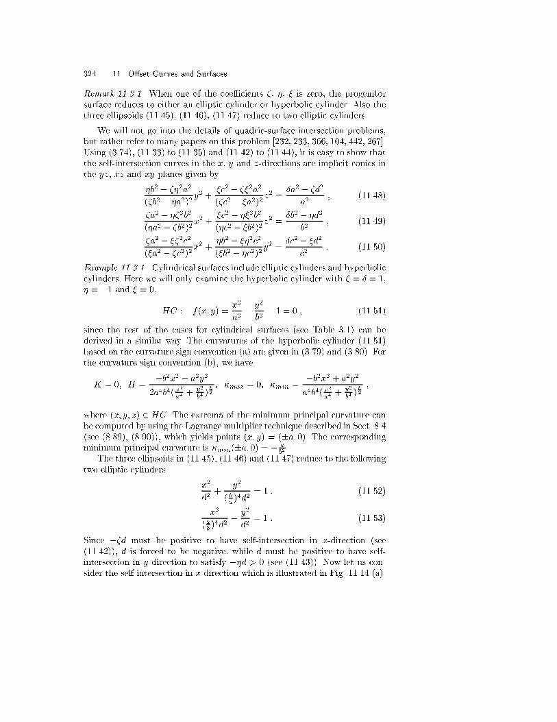
324 11. O�set Curves and Surfaces
Remark 11.3.1. When one of the coe�cients �, �, � is zero, the progenitorsurface reduces to either an elliptic cylinder or hyperbolic cylinder. Also thethree ellipsoids (11.45), (11.46), (11.47) reduce to two elliptic cylinders.
We will not go into the details of quadric-surface intersection problems,but rather refer to many papers on this problem [232, 233, 366, 104, 442, 267].Using (3.74), (11.33) to (11.35) and (11.42) to (11.44), it is easy to show thatthe self-intersection curves in the x, y and z-directions are implicit conics inthe yz, xz and xy-planes given by
�b2 � ��2a2(�b2 � �a2)2 y
2 +�c2 � ��2a2(�c2 � �a2)2 z
2 =�a2 � �d2
a2; (11.48)
�a2 � ��2b2(�a2 � �b2)2x
2 +�c2 � ��2b2(�c2 � �b2)2 z
2 =�b2 � �d2
b2; (11.49)
�a2 � ��2c2(�a2 � �c2)2x
2 +�b2 � ��2c2(�b2 � �c2)2 y
2 =�c2 � �d2
c2: (11.50)
Example 11.3.1. Cylindrical surfaces include elliptic cylinders and hyperboliccylinders. Here we will only examine the hyperbolic cylinder with � = � = 1,� = �1 and � = 0,
HC : f(x; y) =x2
a2� y2
b2� 1 = 0 ; (11.51)
since the rest of the cases for cylindrical surfaces (see Table 3.1) can bederived in a similar way. The curvatures of the hyperbolic cylinder (11.51)based on the curvature sign convention (a) are given in (3.79) and (3.80). Forthe curvature sign convention (b), we have
K = 0; H =�b2x2 + a2y2
2a4b4(x2
a4 +y2
b4 )32
; �max = 0; �min =�b2x2 + a2y2
a4b4(x2
a4 +y2
b4 )32
;
where (x; y; z) 2 HC. The extrema of the minimum principal curvature canbe computed by using the Lagrangemultiplier technique described in Sect. 8.4(see (8.89), (8.90)), which yields points (x; y) = (�a; 0). The correspondingminimum principal curvature is �min(�a; 0) = � a
b2 .The three ellipsoids in (11.45), (11.46) and (11.47) reduce to the following
two elliptic cylinders
x2
d2+
y2
( ba )4d2
= 1 ; (11.52)
x2
(ab )4d2
+y2
d2= 1 : (11.53)
Since ��d must be positive to have self-intersection in x-direction (see(11.42)), d is forced to be negative, while d must be positive to have self-intersection in y-direction to satisfy ��d > 0 (see (11.43)). Now let us con-sider the self-intersection in x-direction which is illustrated in Fig. 11.14 (a).

11.3 O�set surfaces 325
According to Theorem 11.3.1, hyperbolic cylinder (11.51) must intersect theelliptic cylinder (11.52) to have self-intersection in the x-direction. It is ap-parent that these two surfaces will intersect if d � �a, since the minor axisof the elliptic cylinder is d and hyperbolic cylinder intersects the x-axis at(�a; 0). This self-intersection is due to the global distance function property(constriction) of the hyperbola. Similarly the self-intersection in y-direction
occurs if d � b2
a , which corresponds to the maximum concave radius of cur-vature as obtained above.
Figures 11.14 (a) (b) show the cross section of self-intersections of o�setsof a hyperbolic cylinder (with a = 0:8, b = 1) in x-direction with d = �3and in y-direction with d = 3. The thick and thin solid lines represent thehyperbolic cylinder and its o�set. The thick dashed dot lines represents theelliptic cylinders (11.52) and (11.53). Four thin dashed lines emanating fromthe intersections points and intersecting at the self-intersection points of theo�set are the vector dn. The four intersection points between the hyperboliccylinder (11.51) and elliptic cylinder (11.52) in Fig. 11.14 (a), and the four in-tersection points between hyperbolic cylinder (11.51) and the elliptic cylinder(11.53) in Fig. 11.14 (b) are given by �rb2d2 + a4
a2 + b2; �b
2
a
rd2 � a2a2 + b2
!;
�a
2
b
rb2 + d2
a2 + b2; �
ra2d2 � b4a2 + b2
!:
Figure 11.15 shows the self-intersecting o�sets of an elliptic cylinder (with� = � = 1, � = 0, a = 0:6 and b = 0:8) in the x-direction (a) with d = �0:55and in the y-direction (b) with d = �0:9. The four intersection points forboth cases are given by �rb2d2 � a4b2 � a2 ; �b
2
a
ra2 � d2b2 � a2
!;
�a
2
b
rd2 � b2b2 � a2 ; �
rb4 � a2d2b2 � a2
!:
Example 11.3.2. Consider an ellipsoid (with � = � = � = � = 1) of the form
EP : f(x; y; z) =x2
a2+y2
b2+z2
c2� 1 = 0 : (11.54)
The curvatures based on the curvature sign convention (a) are given in (3.82)and (3.83). For the curvature sign convention (b) we have
K =1
a2b2c2�x2
a4 +y2
b4 + z2
c4
�2 ; H = �x2 + y2 + z2 � a2 � b2 � c2
2a2b2c2�x2
a4 +y2
b4 + z2
c4
� 32
; (11.55)
� =�(x2 + y2 + z2 � a2 � b2 � c2)
2a2b2c2�x2
a4 +y2
b4 + z2
c4
� 32
(11.56)
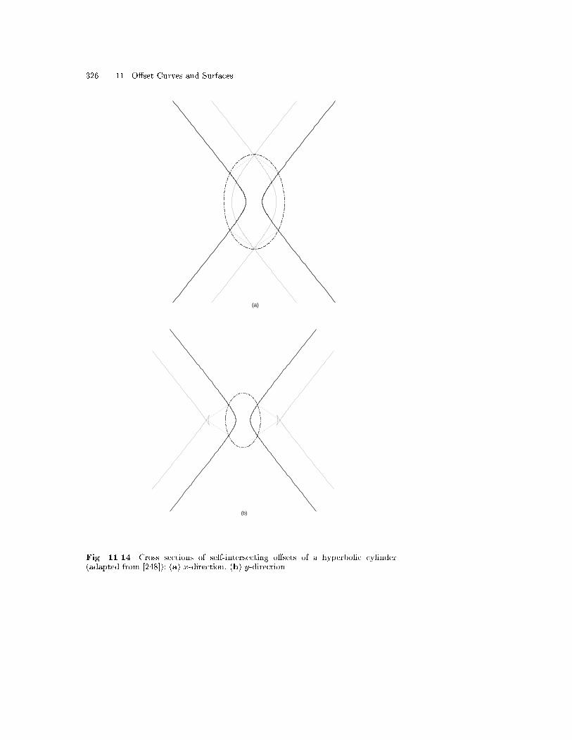
326 11. O�set Curves and Surfaces
(a)
(b)
Fig. 11.14. Cross sections of self-intersecting o�sets of a hyperbolic cylinder(adapted from [248]): (a) x-direction, (b) y-direction

11.3 O�set surfaces 327
(a) (b)
Fig. 11.15. Cross sections of self-intersecting o�sets of an elliptic cylinder (adaptedfrom [248]): (a) x-direction, (b) y-direction
�
r(x2 + y2 + z2 � a2 � b2 � c2)2 � 4a2b2c2
�x2
a4 +y2
b4 + z2
c4
�2a2b2c2
�x2
a4 +y2
b4 + z2
c4
� 32
;
where (x; y; z) 2 EP .The critical points of both principal curvatures can be obtained by using
the Lagrange multiplier technique described in Sect. 8.4 (see (8.89), (8.90)).Since we are assuming a � b � c, the maximum principal curvature hasa global minimum a
b2 at (�a; 0; 0), a local maximum ba2 at (0;�b; 0) and a
global maximum ca2 at (0; 0;�c), while the minimum principal curvature has a
global minimum ac2 at (�a; 0; 0), a local minimum b
c2 at (0;�b; 0) and a globalmaximum c
b2 at (0; 0;�c). Figure 11.16 shows the locations of extrema (black
square), umbilics��aq
b2�a2c2�a2 ; 0; �c
qc2�b2c2�a2
�(white circle), the maximum
principal curvature lines (solid line) and the minimum principal curvaturelines (dotted line).
It is apparent from (11.42) to (11.44) that d must be negative to haveself-intersections in the o�set. First we consider the case of self-intersectionin x-direction. The two ellipsoids EPx and EP will not intersect when EPxis inside EP (jdj < a2
c ), or EP is inside EPx (jdj > a). This leads to the

328 11. O�set Curves and Surfaces
conclusion that EPx and EP intersect if
�a � d � �a2
c:
The magnitude of the upper bound corresponds to the smallest concave ra-dius of curvature at (0; 0;�c), while the magnitude of the lower bound cor-responds to the smallest semi-axis. With a similar discussion, we can derivethe conditions for the self-intersection in the y and z-directions as
y-direction: � b2
a � d � � b2
c ;
z-direction: � c2
a � d � �c :Figure 11.17 shows two ellipsoids EP (with a = 0:6, b = 0:8, c = 1:0)
and EPx ((11.45) with d = �a2
b =-0.45) which is equal to the maximumprincipal radius of curvature at (0;�b; 0), intersecting each other. This is adegenerate intersection of two ellipsoids, consisting of two ellipses, which havethe rational parametrization given by
x(t) = �a2
b
rc2 � b2c2 � a2
1� t21 + t2
; y(t) = b2t
1 + t2; z(t) = �c
2
b
rb2 � a2c2 � a2
1� t21 + t2
;
(11.57)
for �1 � t � 1. The self-intersection curve of the o�set in the yz-plane is anellipse given by
y2
(b2�a2)(a2�d2)a2
+z2
(c2�a2)(a2�d2)a2
= 1 ; (11.58)
which is obtained by substituting � = � = � = � = 1 into (11.48). Figures11.18 show the wireframe of the ellipsoid EP , the intersection curves of twoellipsoids (two ellipses) and pairs of vectors dn emanating from the intersec-tion curves and intersecting in the yz-plane from two di�erent view points.The locus of these intersecting points in (a) is the ellipse (11.58).
Example 11.3.3. Consider an elliptic cone (� = � = 1, � = �1 and � = 0) ofthe form
EC : f(x; y; z) =x2
a2+y2
b2� z2
c2= 0 : (11.59)
The curvatures of the elliptic cone (11.59) based on the curvature sign con-vention (a) are given in (3.85) and (3.86). For the sign convention (b) theyare
K = 0; H =x2 + y2 + z2
2a2b2c2�x2
a4 +y2
b4 + z2
c4
� 32
; (11.60)
�max =x2 + y2 + z2
a2b2c2�x2
a4 +y2
b4 + z2
c4
� 32
; �min = 0 ; (11.61)

11.3 O�set surfaces 329
xy
z
Fig. 11.16. Locations of extrema of principal curvatures (black square), umbilics(white circle) and line of curvatures of ellipsoid (a=0.6, b=0.8, c=1.0) (adaptedfrom [248])
where (x; y; z) 2 EC except at the apex (0,0,0).Since the Gaussian curvature is zero everywhere, the elliptic cone is a
developable surface and hence the minimum principal curvature lines are inthe ruling direction (see Sect. 9.7.1). The maximum principal curvature lines,which are orthogonal to the minimum principal curvature lines, are thus or-thogonal to the ruling directions. Therefore as a point on a ruling approachesthe apex, the maximum principal curvature monotonically increases and willbecome in�nite at the apex.
It is apparent from (11.42) to (11.44) that the o�set of the elliptic coneself-intersects in the x and y-directions if the o�set distance d is negative,while it self-intersects in the z-direction if the o�set distance d is positive.Unlike the case for ellipsoids, all the three ellipsoids intersect with the ellipticcone for all nonzero d, provided the correct sign is chosen. This observationagrees with the result that the maximum principal curvature has an in�nitevalue at the apex.
Figure 11.19 (a) shows the elliptic cone EC (a=0.6, b=0.8 and c=1.0)intersecting the EPx (d=-0.45). The self-intersection curve in the yz-plane is

330 11. O�set Curves and Surfaces
-0.6-0.4-0.200.20.40.6 x
-0.8-0.6
-0.4-0.2
00.2
0.40.6
0.8y
-1
-0.5
0
0.5
1
z
Fig. 11.17. Two intersecting ellipsoids (adapted from [248]): intersection curves,which comprise of two ellipses, represent the footpoint curve of the self-intersectioncurve of o�set of ellipsoid
given by setting � = � = 1; � = �1 and � = 0 into (11.48)
� y2
(b2�a2)d2a2
+z2
(c2+a2)d2
a2
= 1 ; (11.62)
which is a hyperbola. Figure 11.19 (b) shows the wireframe of the ellipticcone EC, the intersection curves of EC and EPx and pairs of vectors dnemanating from the intersection curves and intersecting in the yz-plane. Thelocus of these intersecting points is the hyperbola (11.62).
Theorem 11.3.1 provides a generalized method for obtaining the self-intersection curves of o�sets and the corresponding foot point curves on theprogenitor implicit quadratic surfaces. The theorem is useful for tool pathgeneration for NC machining and other engineering applications.
11.3.4 Self-intersection of o�sets of explicit quadratic surfaces
Although o�set surfaces are widely used in various engineering applications,their degenerating mechanism is not well known in a quantitative manner. We

11.3 O�set surfaces 331
xy
z
(a)
xy
z
(b)
Fig. 11.18. Wireframe of the ellipsoid EP , the intersection curves of two ellipsoids(two ellipses) and pairs of vectors dn emanating from the intersection curves andintersecting on the self-intersection curves, adapted from [248]: (a) view parallel tothe yz-plane, (b) view parallel to the xz-plane
have seen in Sect. 8.3, that any regular surface can be locally approximatedin the neighborhood of a point P by an explicit quadratic surface of the form
r(x; y) = [x; y;1
2(�x2 + �y2)]T ; (11.63)
to the second order where �� and �� are the principal curvatures at pointP . The minus signs are consistent with curvature sign convention (b). There-fore investigations of the self-intersection mechanisms of the o�sets of explicitquadratic surfaces due to di�erential geometry properties lead to an under-standing of the self-intersecting mechanisms of o�sets of regular parametricsurfaces.
In the sequel we assume d > 0, � > 0 and � � � without loss of generality.According to this assumption the surface is a hyperbolic paraboloid when� < 0, an elliptic paraboloid when 0 < � < �, a paraboloid of revolutionwhen 0 < � = �, and a parabolic cylinder when � = 0 as illustrated in Fig.8.9. The paraboloid of revolution and the parabolic cylinder can be consideredas degenerate cases of the elliptic paraboloid. When � = �, the principaldirection is not de�ned and the point (0; 0; 0) will become an umbilic. If �and � vanish at the same time, the surface is part of a plane, and we do notinvestigate such cases.

332 11. O�set Curves and Surfaces
-0.6-0.4-0.200.20.40.6 x
-0.8-0.6-0.4-0.2 00.20.40.60.8y
-1
-0.5
0
0.5
1
z
x
y
z
(a) (b)
Fig. 11.19. (a) Intersection between EC (a = 0:6, b = 0:8, c = 1:0) and EPx
(d = �a2
b=-0.45), (b) wireframe of the elliptic cone EC, the intersection curves of
EC and EPx and pairs of vectors dn emanating from the intersection curves andintersecting on the self-intersection curves (adapted from [248])
In the case for o�sets of explicit quadratic surfaces, there are no self-intersections due to global distance function properties [26], thus if d > 0the maximum absolute value of the negative minimum principal curvaturedetermines the largest o�set d without degeneracy. The largest magnitudeof o�set distance without degeneracy is called the maximum o�set distancejdmaxj. In Sect. 8.3 we discussed how to �nd the global minimum of theminimum principal curvature of explicit quadratic surfaces.
Due to Lemma 8.3.1 the global minimum of the minimum principal cur-vature of the explicit quadratic surface occurs at the origin, except for aparabolic cylinder ((11.63) with �=0) which has minima along the x-axiswith curvature value �min = ��, and hence the maximum o�set distanceis determined to be jdmaxj = 1
� . If the o�set distance exceeds 1� , the o�set
starts to degenerate from the point (0; 0; 1� ) on the o�set surface except fora parabolic cylinder progenitor, where the o�set starts to degenerate alongthe line (x; 0; 1� ).
Substitution of the expression of the o�set of the explicit quadratic surface(11.63)
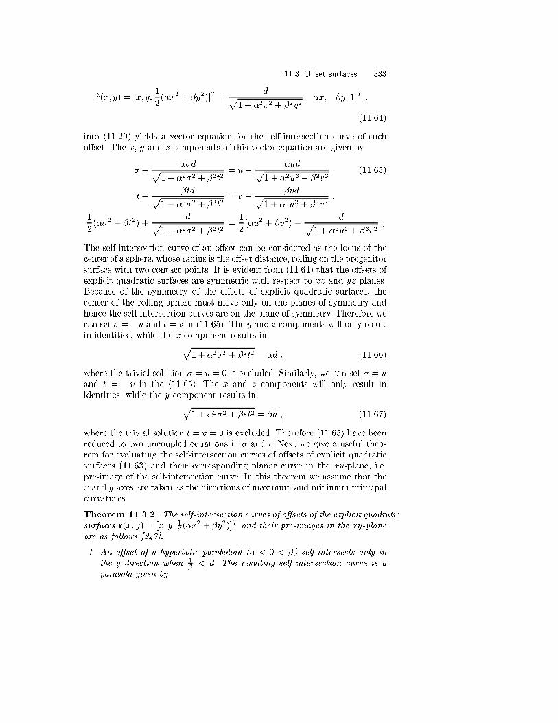
11.3 O�set surfaces 333
r(x; y) = [x; y;1
2(�x2 + �y2)]T +
dp1 + �2x2 + �2y2
[��x;��y; 1]T ;
(11.64)
into (11.29) yields a vector equation for the self-intersection curve of sucho�set. The x, y and z components of this vector equation are given by
� � ��dp1 + �2�2 + �2t2
= u� �udp1 + �2u2 + �2v2
; (11.65)
t� �tdp1 + �2�2 + �2t2
= v � �vdp1 + �2u2 + �2v2
;
1
2(��2 + �t2) +
dp1 + �2�2 + �2t2
=1
2(�u2 + �v2) +
dp1 + �2u2 + �2v2
;
The self-intersection curve of an o�set can be considered as the locus of thecenter of a sphere, whose radius is the o�set distance, rolling on the progenitorsurface with two contact points. It is evident from (11.64) that the o�sets ofexplicit quadratic surfaces are symmetric with respect to xz and yz planes.Because of the symmetry of the o�sets of explicit quadratic surfaces, thecenter of the rolling sphere must move only on the planes of symmetry andhence the self-intersection curves are on the plane of symmetry. Therefore wecan set � = �u and t = v in (11.65). The y and z components will only resultin identities, while the x component results inp
1 + �2�2 + �2t2 = �d ; (11.66)
where the trivial solution � = u = 0 is excluded. Similarly, we can set � = uand t = �v in the (11.65). The x and z components will only result inidentities, while the y component results inp
1 + �2�2 + �2t2 = �d ; (11.67)
where the trivial solution t = v = 0 is excluded. Therefore (11.65) have beenreduced to two uncoupled equations in � and t. Next we give a useful theo-rem for evaluating the self-intersection curves of o�sets of explicit quadraticsurfaces (11.63) and their corresponding planar curve in the xy-plane, i.e.pre-image of the self-intersection curve. In this theorem we assume that thex and y axes are taken as the directions of maximum and minimum principalcurvatures.
Theorem 11.3.2. The self-intersection curves of o�sets of the explicit quadraticsurfaces r(x; y) = [x; y; 12 (�x
2 + �y2)]T and their pre-images in the xy-planeare as follows [247]:
1. An o�set of a hyperbolic paraboloid (� < 0 < �) self-intersects only inthe y-direction when 1
� < d. The resulting self-intersection curve is aparabola given by
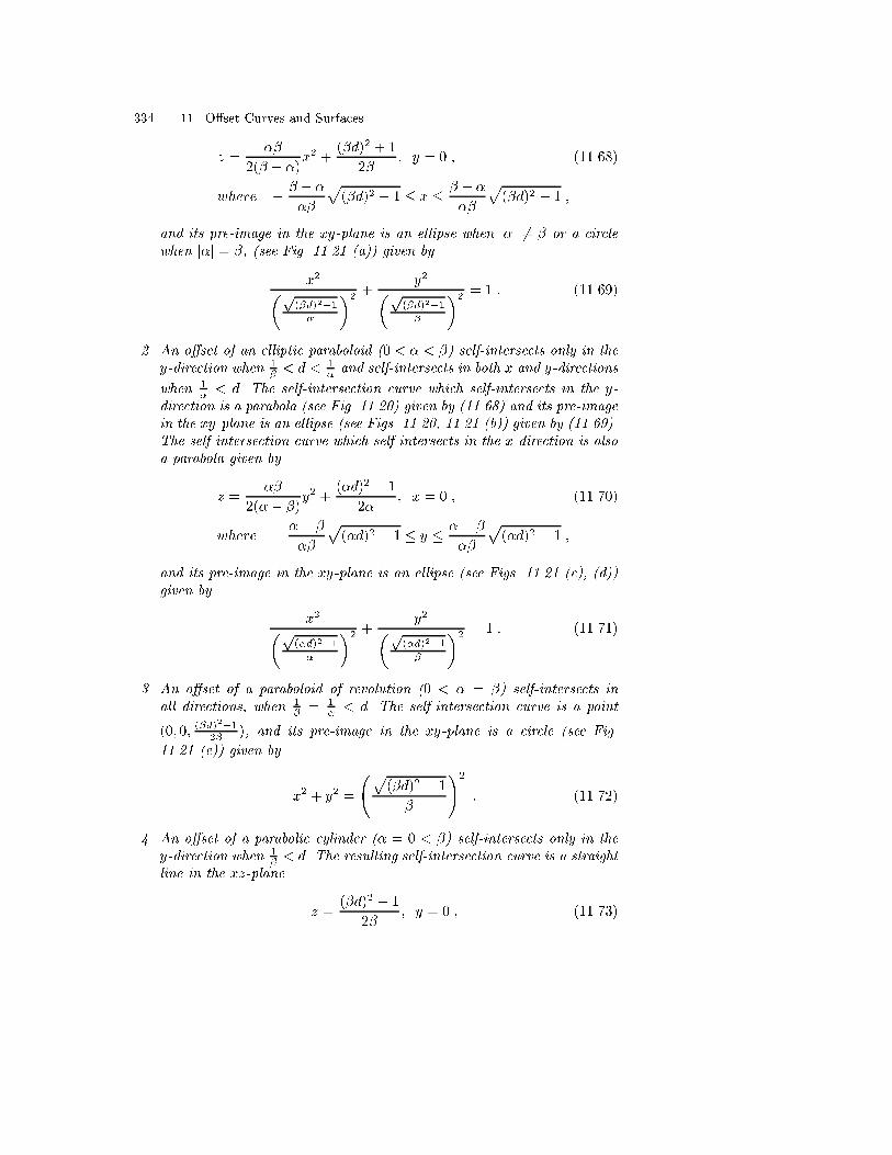
334 11. O�set Curves and Surfaces
z =��
2(� � �)x2 +
(�d)2 + 1
2�; y = 0 ; (11.68)
where � � � ���
p(�d)2 � 1 � x � � � �
��
p(�d)2 � 1 ;
and its pre-image in the xy-plane is an ellipse when j�j 6= � or a circlewhen j�j = �, (see Fig. 11.21 (a)) given by
x2�p(�d)2�1
�
�2 +y2�p
(�d)2�1
�
�2 = 1 : (11.69)
2. An o�set of an elliptic paraboloid (0 < � < �) self-intersects only in they-direction when 1
� < d < 1� and self-intersects in both x and y-directions
when 1� < d. The self-intersection curve which self-intersects in the y-
direction is a parabola (see Fig. 11.20) given by (11.68) and its pre-imagein the xy-plane is an ellipse (see Figs. 11.20, 11.21 (b)) given by (11.69).The self-intersection curve which self-intersects in the x-direction is alsoa parabola given by
z =��
2(�� �)y2 +
(�d)2 + 1
2�; x = 0 ; (11.70)
where � �� ���
p(�d)2 � 1 � y � �� �
��
p(�d)2 � 1 ;
and its pre-image in the xy-plane is an ellipse (see Figs. 11.21 (c), (d))given by
x2�p(�d)2�1
�
�2 +y2�p
(�d)2�1
�
�2 = 1 : (11.71)
3. An o�set of a paraboloid of revolution (0 < � = �) self-intersects inall directions, when 1
� = 1� < d. The self-intersection curve is a point
(0; 0; (�d)2�1
2� ), and its pre-image in the xy-plane is a circle (see Fig.
11.21 (e)) given by
x2 + y2 =
p(�d)2 � 1
�
!2
: (11.72)
4. An o�set of a parabolic cylinder (� = 0 < �) self-intersects only in they-direction when 1
� < d. The resulting self-intersection curve is a straightline in the xz-plane
z =(�d)2 � 1
2�; y = 0 ; (11.73)

11.3 O�set surfaces 335
and its pre-image in the xy-plane (see Fig. 11.21 (f)) are two straightlines given by
y = �p(�d)2 � 1
�: (11.74)
Proof:Case (1): Since � is negative for the hyperbolic paraboloid and we are assum-ing d > 0 and the left hand side of (11.66) is always positive, this equationcannot be used to derive the self-intersection curve. This implies that theo�set of a hyperbolic paraboloid does not self-intersect in the x-direction(maximum principal direction). However, we can use (11.67) to derive theself-intersection curve in the y-direction (minimum principal direction). Uponsquaring and replacing � by x and t by y we obtain
�2x2 + �2y2 = (�d)2 � 1 : (11.75)
This equation describes an ellipse in the xy-plane and is equivalent to (11.69).Since the left hand side of (11.75) is always positive, the equation is only validwhen 1
� < d. This indicates that there is no self-intersection unless the o�set
distance exceeds the maximum o�set distance jdmaxj = 1� . Now we can obtain
the self-intersection curve in the xz-plane by mapping the ellipse in xy-plane(see (11.75)) into the 3-D coordinates using (11.64), resulting in:
r(x; y) = [x(x; y); y(x; y); z(x; y)]T
= [(� � ��
)x; 0;1
2�f�(� � �)x2 + (�d)2 + 1g]T ; (11.76)
where �p
(�d)2�1
� � x �p
(�d)2�1
� . The range of parameter x comes from(11.75). If we eliminate the parameter x from (11.76) and replace x by x andz by z, we obtain the same result as (11.68).
Case (2): Since � is positive for the elliptic paraboloid, both (11.66),(11.67) can be used to obtain the self-intersection curves in the xy-plane.This implies that the o�set of an elliptic paraboloid may self-intersect in bothprincipal directions. Since we have already derived the equation from (11.67),we derive another equation from (11.66). Upon squaring and replacing � byx and t by y we obtain
�2x2 + �2y2 = (�d)2 � 1 ; (11.77)
which is equivalent to (11.71). Also this equation is only valid when 1� < d.
The self-intersection curve in 3-D coordinates can easily be obtained in asimilar manner with Case (1).
Case (3): If we set � = � in (11.75) and (11.77), both equations reduceto (11.72). Also if we set � = � in (11.76), the parabola reduces to the point
(0; 0; (�d)2+1
2� ).
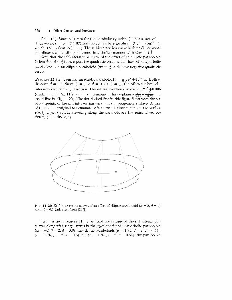
336 11. O�set Curves and Surfaces
Case (4): Since � is zero for the parabolic cylinder, (11.66) is not valid.Thus we set � = 0 in (11.67) and replacing t by y we obtain �2y2 = (�d)2�1,which is equivalent to (11.74). The self-intersection curve in three dimensionalcoordinates can easily be obtained in a similar manner with Case (1).
Note that the self-intersection curve of the o�set of an elliptic paraboloid(when 1
� < d < 1� ) has a positive quadratic term, while those of a hyperbolic
paraboloid and an elliptic paraboloid (when 1� < d) have negative quadratic
terms.
Example 11.3.4. Consider an elliptic paraboloid z = 12 (2x
2+4y2) with o�setdistance d = 0:3. Since 1
� = 14 < d = 0:3 < 1
2 = 1� , the o�set surface self-
intersects only in the y-direction. The self-intersection curve is z = 2x2+0:305
(dashed line in Fig. 11.20) and its pre-image in the xy-plane is x2
0:11+y2
0:0275 = 1(solid line in Fig. 11.20). The dot dashed line in this �gure illustrates the setof footpoints of the self-intersection curve on the progenitor surface. A pairof thin solid straight lines emanating from two distinct points on the surfacer(�; t), r(u; v) and intersecting along the parabola are the pairs of vectorsdN(�; t) and dN(u; v).
x
y z
Fig. 11.20. Self-intersection curves of an o�set of elliptic paraboloid (� = 2, � = 4)with d = 0:3 (adapted from [247])
To illustrate Theorem 11.3.2, we plot pre-images of the self-intersectioncurves along with ridge curves in the xy-plane for the hyperbolic paraboloid(� = �2, � = 2, d = 0:6), the elliptic paraboloids (� = 1:75, � = 2, d = 0:55),(� = 1:75, � = 2, d = 0:6) and (� = 1:75, � = 2, d = 0:65), the paraboloid

11.3 O�set surfaces 337
(� = b = 2, d = 0:6) and the parabolic cylinder (� = 0, � = 2, d = 0:6) asdepicted in Figs. 11.21 (a) to (f).
It is interesting to note that when the progenitor surface is a hyperbolicparaboloid or an elliptic paraboloid (see Fig. 11.21 (a) to (d)), the pre-imagesof the self-intersection curve of its o�set which self-intersects in the y-directionand the ridge curve �min(x; y) = � 1
d always intersect tangentially at y =0. The pre-image of the self-intersection curve of the o�set of an ellipticparaboloid (see Fig. 11.21 (c)), which self-intersects in x-direction, and theridge curve �max(x; y) = � 1
d intersect tangentially at x = 0, when the tworidge curves intersect with the y-axis within the two umbilics. Whereas whenthe two ridge curves intersect the y-axis outside the two umbilics (see Fig.11.21 (d)), the pre-images of the self-intersection curve and the ridge curve�min(x; y) = � 1
d intersect tangentially at x = 0.It is apparent from (11.21) that the direction of the normal vector of the
o�set surface is opposite to that of the progenitor surface inside the loop of�min(x; y) = � 1
d (dashed line) in the absence of the loop of �max(x; y) = � 1d
(see Figs. 11.21 (a), (b), (e)), and the regions between outside the loop of�max(x; y) = � 1
d (dot dot dashed line) and inside the loop of �min(x; y) = � 1d
(see Figs. 11.21 (c), (d)), while the direction is the same within the loop of�max(x; y) = � 1
d (see Figs. 11.21 (c), (d)).Figures 11.22, 11.23 and 11.24 show self-intersecting o�set surfaces, self-
intersection and ridge curves in 3-D space and the trimmed o�set surface ofa hyperbolic paraboloid (� = �2, � = 2, d = 0:6), an elliptic paraboloid(� = 1:75, � = 2, d = 0:6) and an elliptic paraboloid (� = 1:75, � = 2,d = 0:65), respectively.
Figure 11.25 illustrates the self-intersections of the o�set of a bicubicB�ezier surface patch. Figure 11.25 (a) shows the pre-images of the self-intersection curve in the parameter domain. The thick line represents thenumerically traced self-intersection curve, while the thin line represents theellipses of (11.69), (11.71), which are in quite good agreement. The same bul-let symbols are mapped to the same locations on the o�set surface. Figure11.25 (b) shows the mapping of the self-intersection curves in the parameterdomain onto the progenitor surface. Finally, Fig. 11.25 (c) shows the o�setsurface with its self-intersections.
11.3.5 Self-intersection of o�sets of polynomial parametric surfacepatches
For parametric surface patches r(u; v) = (x(u; v); y(u; v); z(u; v))T , the unitnormal vector of a regular surface (3.3) in terms of components is given by
N(u; v) =(yuzv � yvzu; xvzu � xuzv; xuyv � xvyu)Tp
(yuzv � yvzu)2 + (xvzu � xuzv)2 + (xuyv � xvyu)2
��Nx(u; v)
S(u; v);Ny(u; v)
S(u; v);Nz(u; v)
S(u; v)
�T; (11.78)

338 11. O�set Curves and Surfaces
(a) x
y
-0.67 -0.33 0.00 0.33 0.67 -0.50
-0.17
0.17
0.50
(b) x
y
-0.67 -0.33 0.00 0.33 0.67 -0.50
-0.17
0.17
0.50
(c) x
y
-0.67 -0.33 0.00 0.33 0.67 -0.50
-0.17
0.17
0.50

11.3 O�set surfaces 339
(d) x
y
-0.67 -0.33 0.00 0.33 0.67 -0.50
-0.17
0.17
0.50
(e) x
y
-0.67 -0.33 0.00 0.33 0.67 -0.50
-0.17
0.17
0.50
(f) x
y
-0.67 -0.33 0.00 0.33 0.67 -0.50
-0.17
0.17
0.50
Fig. 11.21. Pre-images of self-intersection curves and ridge curves of o�sets ofexplicit quadratic surfaces (adapted from [247]). The solid lines correspond to pre-images of the self-intersection curves for self-intersection in the y-direction. Thedashed lines correspond to �min(x; y) = � 1
d. The dot dashed lines correspond to
pre-images of the self-intersection curves for self-intersection in the x-direction. Thedot dot dashed lines correspond to �max(x; y) = � 1
d. Symbols � and � represent the
locations of generic lemon type umbilics and non-generic umbilics, respectively. (a)Hyperbolic paraboloid (� = �2, � = 2, d = 0:6), (b) elliptic paraboloid (� = 1:75,� = 2, d = 0:55), (c) elliptic paraboloid (� = 1:75, � = 2, d = 0:6), (d) ellipticparaboloid (� = 1:75, � = 2, d = 0:65), (e) paraboloid of revolution (� = � = 2,d = 0:6), (f) parabolic cylinder (� = 0, � = 2, d = 0:6)

340 11. O�set Curves and Surfaces
Fig. 11.22. Self-intersecting o�set surface (top), region bounded by self-intersection curve (middle) and trimmed o�set surface (bottom) of a hyperbolicparaboloid z = 1
2(�2x2 + 2y2) with d = 0:6 (adapted from [247])
where Nx, Ny and Nz denote the x, y and z components of ru � rv andS = jru � rv j. Consequently the vector equation for self-intersections (11.29)becomes
x(�; t) +Nx(�; t)
S(�; t)d = x(u; v) +
Nx(u; v)
S(u; v)d ; (11.79)
y(�; t) +Ny(�; t)
S(�; t)d = y(u; v) +
Ny(u; v)
S(u; v)d ; (11.80)
z(�; t) +Nz(�; t)
S(�; t)d = z(u; v) +
Nz(u; v)
S(u; v)d ; (11.81)
which is an underconstrained system with three equations with four un-knowns �, t, u, v.
We can easily trace any self-intersection curve branch if the pre-imageof that branch in at least one of the parametric domains starts from theparametric domain boundary as depicted in Fig. 11.26 (a). The same symbolsin �t and uv-parameter spaces are the corresponding pairs of points whichgive the self-intersection. It is more di�cult to �nd starting points for tracingself-intersection curves, when the self-intersections curves are closed in bothparametric domains as illustrated in Fig. 11.26 (b). This may occur due tolocal di�erential geometry properties and global distance function properties

11.3 O�set surfaces 341
Fig. 11.23. Self-intersecting o�set surface (top), region bounded by self-intersection curves (middle) and trimmed o�set surface (bottom) of ellipticparaboloid z = 1
2(1:75x2 + 2y2) with d = 0:6 (adapted from [247])
of the progenitor surface. The �rst case occurs in the vicinity of extrema ofprincipal curvatures in a concave region, when the o�set distance exceedsthe smallest radius of curvature [252]. The second case occurs in the vicinityof a pair of collinear normal points whose distance is equal or smaller thantwice the o�set distance. If the surface is conceptually subdivided along aniso-parametric line which contains the local extrema of principal curvaturein the concave region (whose radius of curvature is smaller than the absoluteo�set distance jdj) or the collinear normal points whose distance is equal orsmaller than twice the o�set distance, then each sub-patch will contain simpleself-intersection branches without loops.
Therefore after this subdivision process, we can �nd all the starting pointsfor tracing self-intersection curves of an o�set surface along iso-parametriclines made up of the boundary of all subdomains. Since we can �x one of

342 11. O�set Curves and Surfaces
Fig. 11.24. Self-intersecting o�set surface (top), region bounded by self-intersection curves (middle) and trimmed o�set surface (bottom) of ellipticparaboloid z = 1
2(1:75x2 + 2y2) with d = 0:65 (adapted from [247])
the four variables (�, t, u, v), the vector equation (11.29) reduces to threeequations with three unknowns.
Let us assume that the input curve is a B�ezier patch. Then the system(11.79), (11.80), (11.81) reduces to three simultaneous trivariate irrationalequations involving polynomials and square root of polynomials. We can re-place the square root of polynomials S(�; t) and S(u; v) by auxiliary variables� and � such that �2 = S2(�; t) and �2 = S2(u; v). Consequently, the abovesystem can be reduced to a nonlinear polynomial system consisting of �veequations with �ve unknowns as follows:
��[x(�; t) � x(u; v)] + d[�Nx(�; t) � �Nx(u; v)] = 0 ; (11.82)
��[y(�; t) � y(u; v)] + d[�Ny(�; t) � �Ny(u; v)] = 0 ; (11.83)
��[z(�; t) � z(u; v)] + d[�Nz(�; t) � �Nz(u; v)] = 0 ; (11.84)
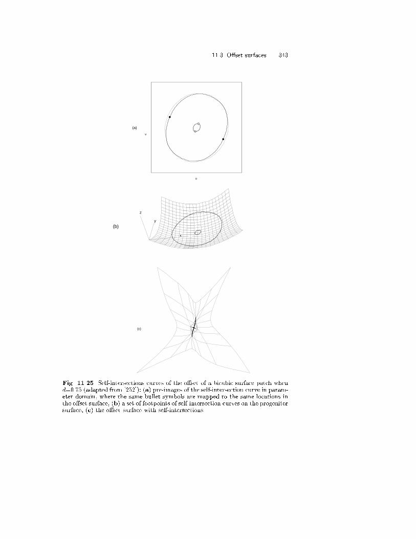
11.3 O�set surfaces 343
u
v
(a)
x
y
z
(b)
(c)
Fig. 11.25. Self-intersections curves of the o�set of a bicubic surface patch whend=0.75 (adapted from [252]): (a) pre-images of the self-intersection curve in param-eter domain, where the same bullet symbols are mapped to the same locations inthe o�set surface, (b) a set of footpoints of self-intersection curves on the progenitorsurface, (c) the o�set surface with self-intersections

344 11. O�set Curves and Surfaces
σ
t
u
v
σ
t
u
v
(a)
(b)
o
+
+
o
+ o
+
o
Fig. 11.26. Self-intersection curves in parameter space where the same symbolsare mapped to the same locations in the o�set surface (adapted from [252])
�2 �N2x(�; t) �N2
y (�; t)�N2z (�; t) = 0 ; (11.85)
�2 �N2x(u; v)�N2
y (u; v)�N2z (u; v) = 0 : (11.86)
This system can be solved by the IPP method introduced in Chap. 4. Since� = u, t = v are trivial solutions, we must exclude them from the system,otherwise a Bernstein subdivision-based IPP algorithm would attempt tosolve for an in�nite number of roots.
A similar problem for the self-intersections of a normal o�set of a planarpolynomial curve has been treated in [253] by dividing out the common factor.However, for the surface case we cannot divide out these factors from thesystem directly, since terms x(�; t) � x(u; v), y(�; t) � y(u; v) and z(�; t) �z(u; v) do not necessarily exactly involve the factors � � u and t � v. Thus,the polynomial system is �rst solved by the Bernstein subdivision-based IPPsolver with a coarse accuracy (e.g. 10�1 � 10�2). The two rectangular sub-patches on the surface for each set of roots using the de Casteljau subdivision

11.3 O�set surfaces 345
algorithm are extracted. Then the normal rectangular pyramids [207, 208,381], which bound normal vectors of B�ezier patches, are constructed [252] andtheir apexes are translated to the origin. If the two pyramids intersect, theassociated parameter boxes are considered as representing trivial roots andexcluded from the list of roots. Figures 11.27 illustrate such non-intersectingand intersecting normal pyramids. Finally we restart the IPP solver withboxes that include the solutions but now requiring high accuracy (e.g. 10�8).
When the input surface is a B-spline surface patch, we can split it intoB�ezier surface patches by the knot insertion algorithm [34, 63, 313]. In suchcases we must check the intersections among the o�sets of di�erent splitpatches, where we do not need to worry about trivial solutions. Wang [439]computed intersection curves of o�sets of two parametric surface patchesusing the orthogonal projection of the intersection curves onto the progenitorsurfaces.
x
y
z
x
y
z
(a) (b)
Fig. 11.27. Normal pyramids: (a) two non-intersecting normal pyramids, (b) twointersecting normal pyramids (adapted from [252])
11.3.6 Tracing of self-intersection curves
Di�erential equations for tracing self-intersection curves of an o�set surfacewere �rst derived by Aomura and Uehara [11]. They are formulated suchthat the self-intersection curve is arc length parametrized in the parameterdomain of the progenitor surface. Here we derive a set of ordinary di�erential

346 11. O�set Curves and Surfaces
equations following the method we introduced in Sect. 5.8.2 for tracing thesurface to surface intersection curves. The tracing direction coincides withthe tangential direction of the self-intersection curve c(s) of the o�set surfacewhich is perpendicular to the two normal vectors at the corresponding footpoints on the progenitor surfaces r(�; t) and r(u; v) where (�; t) 6= (u; v).Therefore, the tracing direction can be obtained as follows:
c0(s) =S(�; t)� S(u; v)jS(�; t)� S(u; v)j ; (11.87)
where S(�; t) and S(u; v) are the normal vectors
S(u; v) = ru � rv ; (11.88)
evaluated at r(�; t) and r(u; v) where (�; t) 6= (u; v) and jS(�; t) � S(u; v)j 6=0. The normalization of the tangent vector forces c(s) to be arc lengthparametrized in R3.
The self-intersection curve of an o�set surface can be also viewed as acurve on the o�set surface. If we denote the pair of the self-intersection curvesin the parameter domain of the progenitor surface as u = �(s), v = t(s) andu = u(s), v = v(s), where s denotes the arc length on the o�set surface, thenthe self-intersection curve on the o�set can be expressed as
r = c(s) = r(�(s); t(s)) = r(u(s); v(s)) : (11.89)
We can derive the unit tangent vector of the self-intersection curve as a curveon the o�set surface using the chain rule as:
c0(s) = ru(�(s); t(s))�0 + rv(�(s); t(s))t
0 ; (11.90)
c0(s) = ru(u(s); v(s))u0 + rv(u(s); v(s))v
0 : (11.91)
Since we know the unit tangent vector of the intersection curve from(11.87), we can �nd �0 and t0 as well as u0 and v0 by taking the dot productof both sides of (11.90) with ru(�(s); t(s)) and rv(�(s); t(s)) and of (11.91)with ru(u(s); v(s)) and rv(u(s); v(s)), which leads to linear systems in �0,t0 and u0, v0. The solutions to the two linear systems have the same formexcept that they are evaluated at di�erent parameter values (�(s); t(s)) and
(u(s); v(s)). Using the relation between N and N (11.19), the ordinary dif-ferential equations for tracing the self-intersection curve of an o�set surfaceare given by
�0 =det(c0; rv ;S)
S2(1 + 2Hd+Kd2) (�(s);t(s)); (11.92)
t0 =det(ru; c
0;S)S2(1 + 2Hd+Kd2) (�(s);t(s))
; (11.93)

11.3 O�set surfaces 347
u0 =det(c0; rv ;S)
S2(1 + 2Hd+Kd2) (u(s);v(s)); (11.94)
v0 =det(ru; c
0;S)S2(1 + 2Hd+Kd2) (u(s);v(s))
: (11.95)
Figure 11.28 illustrates the global self-intersection of an o�set withoutloops. As depicted in Fig. 11.28 the surface has a global constriction betweentwo corner points and the o�set surface self-intersects globally without anyinternal loops. The self-intersection curves can be traced by starting at thesurface boundary.
The next example, in Fig. 11.29, shows global self-intersection with loops.The surface also has 4 pairs of collinear normal point with distances 0.3757,0.3945, 0.1367, 0.3757. Therefore if the magnitude of the o�set distance ex-ceeds 0:1367
2 , two self-intersection loops start to grow in the parameter domainenclosing the pair of collinear normal points whose distance in R3 is 0.1367[252].
11.3.7 Approximations
Farouki [94] studied the problem of computing approximate o�sets of generalparametric surfaces. His method involves �nding the unique bicubic Hermiteinterpolant surface that has the exact position, slopes and cross-derivativesas the exact o�set surface at the corners of some quadrilateral subdomainof the surface being o�set. The accuracy of the o�set is then increased bydecreasing the size of the subdomain chosen. A uniform subdivision methodsis implemented, although a nonuniform subdivision can be formulated toenhance the e�ciency.
Patrikalakis and Prakash [300] addressed the representation of plateswithin the framework of the boundary representation method in a solid mod-eling environment (see Figure 11.5). Plates are de�ned as the volume boundedby a progenitor surface, its o�set surface and ruled surfaces for the sides.O�set surfaces of rational B-spline/B�ezier surfaces cannot in general be rep-resented exactly within the same class of functions describing the progenitorsurface. Therefore, if the o�set is to be represented in the same form as theprogenitor surface, approximation is required. Such approximation assists inintegrating o�sets in a NURBS-based modeler (at least in an approximatesense).
The steps of the approximation algorithm in [300] are summarized below.
1. Let R be a progenitor rational B-spline surface with control vertices pij ,weights wij >0 and two knot vectors U and V associated with eachparameter u and v.
2. O�set each vertex of the control polyhedron by a distance d along thenormal vector given by (see Fig. 11.30)

348 11. O�set Curves and Surfaces
v
u
(a)
x
y
z
(b)
x
y
z
(c)
Fig. 11.28. Self-intersection curves of the o�set of a bicubic surface patch whend=0.09 (adapted from [252]): (a) pre-images of the self-intersection curves in pa-rameter domain where the same symbols are mapped to the same points in theo�set surface, (b) the mapping of the self-intersection curves in the parameter do-main onto the progenitor surface, (c) the o�set surface and the self-intersectioncurve

11.3 O�set surfaces 349
u
v
(a)
xy
z
(b)
x
y
z
(c)
Fig. 11.29. Self-intersection curves of the o�set of a bisextic surface patch whend=-0.08 (adapted from [252]): (a) pre-images of the self-intersection curves in pa-rameter domain where the same symbols are mapped to the same points in theo�set surface, (b) the mapping of the self-intersection curves in the parameter do-main onto the progenitor surface, (c) the o�set surface and the self-intersectioncurve

350 11. O�set Curves and Surfaces
Nij =1
8
8Xk=1
nk ; (11.96)
so that the o�set control point is given by
pij = pij + dNij
jNij j ; (11.97)
where nk are unit normal vectors on the triangular facets of the controlpolyhedron around Pij as in Fig. 11.30. Then the approximated o�set Ris de�ned by pij , wij , U and V.
3. Check deviation of the approximate o�set with the true o�set for every(ui; vj) 2 U�V. If it is good at all points, the checking proceeds to thenext stage. If it is not good at some point, then new knots are addedat left and right midspans of both the u and v-directions. Knots are notadded at those points where a new knot has been currently added to avoidunnecessary knots that could, possibly, lower the order of continuity. Inthe second stage, the surface is further checked progressively at its u andv midspans, one-third spans, etc., to some prespeci�ed level of interiorchecking. A new u and v knot is added at places where the check fails. Ifthe check passes at all points, the approximate o�set is considered goodenough.
4. Evaluate a new control polyhedron corresponding to the �ner knot vectorusing the Oslo algorithm [63] and go back to step 2.
Nij
n k
Nij = (1/8)Σ nk=1
8
k Fig. 11.30. O�set surface ap-proximation (adapted from [300])
An alternate way to compute o�sets of NURBS curves and surfaces wasaddressed by Piegl and Tiller [315]. The approach consists of four steps: 1)recognition of special curves such as a straight line or a circle, and specialsurfaces such as a plane, a surface of revolution (sphere, torus, cone, cylinder)
11.4 Pythagorean hodograph 351
or a general surface of revolution, or a ruled surface which in special cases canbe an extrusion; 2) sampling of the o�set curve or surface based on boundson second derivatives; 3) interpolation of these points by B-spline curves andsurfaces; 4) removal of all extraneous knots so that the error does not exceedthe tolerance.
11.4 Pythagorean hodograph
11.4.1 Curves
Farouki and Sakkalis [108] introduced a class of special planar polynomialcurves called Pythagorean hodograph (PH) curves r(t) = (x(t); y(t))T , whosehodograph (derivative) components _x(t), _y(t) and a polynomial �(t) form aPythagorean triple _x2(t)+ _y2(t) = �2(t). Thus, the PH curve has polynomialparametric speed �(t); accordingly its o�set is a rational curve and its arclength is a polynomial function s(t) of the parameter t. The Pythagoreancondition is satis�ed by
_x(t) = (a2(t)� b2(t))c(t); _y(t) = 2a(t)b(t)c(t); �(t) = (a2(t) + b2(t))c(t) ;
(11.98)
where a(t), b(t) and c(t) are polynomials satisfying GCD(a; b) = 1 andmax(deg(a); deg(b)) � 1 [108, 114] where GCD denotes greatest commondivisor. This condition is only a su�cient condition for a polynomial curve tohave rational o�set. For most applications c(t) is chosen to be 1. The lowestdegree PH curve occurs when the polynomials a(t) and b(t) are linear andthus from (11.98) its degree is cubic. However, the resulting PH curve cannotpossess an in ection point and hence is not practical. When a(t) and b(t) arequadratic, the PH curve will be a quintic and is the lowest degree curve tohave enough exibility for practical use. The PH quintics can in ect and caninterpolate arbitrary �rst-order Hermite data [103]. The degree of the o�setis 2m� 1 for a degree m PH curve. Therefore, the lowest degree of the o�setof a PH curve for practical use is nine.
Farouki and Shah [112] developed a real-time CNC interpolator for PHcurves using the fact that the arc length s(t) of a PH curve is a polynomialfunction. As a consequence the generation of reference points along a PHcurve is reduced to a sequence of polynomial root�nding problems.
The planar PH curves can be easily generalized to space PH curves [110]by setting the four real polynomials a(t), b(t), c(t), "(t) in the form
_x(t) = (a2(t)� b2(t)� c2(t))"(t); _y(t) = 2a(t)b(t)"(t); _z(t) = 2a(t)c(t)"(t) ;
(11.99)
which leads to a polynomial parametric speed �(t) = (a2(t)+b2(t)+c2(t))"(t).A more thorough review of PH curves can be found in [114].

352 11. O�set Curves and Surfaces
Pottmann [323] generalized the concept of PH curves to the full class ofrational curves with rational o�sets, by utilizing the projective dual repre-sentation. A rational planar curve is obtained as the envelope of its tangentline which is described as
g(t) : nx(t)x+ ny(t)y = h(t) ; (11.100)
where h(t) is the signed distance of the tangent line g(t) from the origin andis a rational function. The vector (nx(t); ny(t))
T is a rational unit normal ofthe tangent line g(t) and is given by
nx(t) =2a(t)b(t)
a2(t) + b2(t); ny(t) =
a2(t)� b2(t)a2(t) + b2(t)
; (11.101)
where (11.98) is used so that the unit normal vector becomes rational. Theenvelope of the one-parameter family of g(t) can be obtained by solving alinear system consisting of (11.100) and its derivative _g(t) for x and y as afunction of t, resulting in:
(x(t); y(t)) =
�X(t)
W (t);Y (t)
W (t)
�; (11.102)
where
X = 2ab( _ab� a_b)ef � 1
2(a4 � b4)( _ef � e _f) ;
Y = (a2 � b2)( _ab� a_b)ef + ab(a2 + b2)( _ef � e _f) ;W = (a2 + b2)( _ab� a_b)f2 : (11.103)
Here the rational function h(t) is replaced by e(t)f(t) . The o�set to (11.102) is
obtained by simply replacing h(t) by h(t) + d or equivalently e(t) by e(t) +f(t)d, and thus the degree of the o�set remains the same as that of (11.102),which is an advantage over PH curves. The rational B�ezier representationcan be easily derived by prescribing the polynomials a(t), b(t), e(t) and f(t)and expressing the resulting polynomials X , Y and W in Bernstein form.
The form of (11.102) and (11.103) becomes simpler if the dual B�ezierrepresentation is used [323]. A plane dual B�ezier curve is de�ned by a familyof tangent lines which has the form
U(t) = (uo(t);u1(t);u2(t))T =
nXi=0
UiBi;n(t) ; (11.104)
where Ui are the B�ezier lines (constant line vectors) and Bi;n(t) is the i-thBernstein polynomial of degree n. A line vector U = (uo;u1;u2)
T determinesa straight line uo + u1x+ u2y = 0. From the homogeneous representation of(11.100) in the form, uoW +u1X+u2Y = 0, the dual representation in termsof projective geometry is given by

11.4 Pythagorean hodograph 353
uo : u1 : u2 = �(a2 + b2)e : 2abf : (a2 � b2)f : (11.105)
When f has a factor a2 + b2, there exists a common divisor in the dualrepresentation, thus it is convenient to set f = (a2 + b2)p which leads to
uo : u1 : u2 = �e : 2abp : (a2 � b2)p : (11.106)
The control lines Ui in (11.104) are easily obtained by expressing (11.106) inBernstein form.
L�u [237] showed that the o�set to a parabola is rational; its singular pointat in�nity was studied by Farouki and Sederberg [111]. In [237] L�u provedthat although the o�set (to a parabola) is not rational in the parametert, it may be expressed as a rational form in a new parameter, say u, via aparameter transformation. The reparametrizing function t = t(u) is a rational
function of the form t = f(u)u where f(u) is a quadratic polynomial in u.
The transformed curve �x(u) = x(t(u)), �y(u) = y(t(u)) is not parametrizedproperly, since there are two values of u, which are the roots of the quadraticequation f(u) � tu = 0, for each corresponding point (x; y) = (x(t); y(t)).While the curve �r(u) is traced twice in opposite directions as u increasesfrom �1 to 0 and from 0 to +1, �r(u)+ �n(u)d de�nes a two-sided o�set, i.e.the inward o�set for u < 0 and the outward o�set for u > 0. The resultingrational curve is of degree 6. L�u [238] further derives a necessary and su�cientcondition for a polynomial or more generally rational planar parametric curveto have rational parametric speed.
11.4.2 Surfaces
Pottmann [323] applied the same principle of the rational curve with rationalo�sets to the rational surface with rational o�sets. While the tangent linesare used in the curve case, a two-parametric set of tangent planes
g(u; v) : Nx(u; v)x+Ny(u; v)y +Nz(u; v)z = h(u; v) ; (11.107)
is used for the surface, where (Nx; Ny; Nz)T is a rational unit normal of the
tangent plane and h(u; v) is a rational distance function from the origin. Therest of the discussions are analogous to the curve case.
A developable surface has a constant tangent plane along a generator.Therefore its tangent plane depends on only one parameter, say u. In otherwords, a developable surface can be considered as the envelope of a oneparameter family of planes g(u). The cross product of the normal vectors ofthe two planes g(u) and _g(u) provides a vector of the generator at parameteru. An explicit representation of rational developable surfaces with rationalo�sets has also been given in [323].
L�u [239] studied the rationality of o�sets of quadrics. The key idea is totransform the problem of rational o�sets of quadrics to a simple problemon the rationality of a cubic algebraic surface and use existing results in

354 11. O�set Curves and Surfaces
algebraic geometry [361]. He showed that the o�sets of paraboloids, ellipsoidsand hyperboloids can be rationally parametrized, while cylinders and conesexcept for parabolic cylinders, cylinders of revolution and cones of revolutiondo not possess any rational o�set.
Pottmann et al. [326] proved that o�sets of a nondevelopable rationalruled surface in the whole space always admit a rational parametrization.Even though the o�sets to ruled surfaces are rational in the whole space wherethey are de�ned, the o�set patch to a rational patch may not be expressibleas a rational patch. Therefore, further research is needed for applying thistechnique to a �nite patch.
Peternell and Pottmann [307] construct PH surfaces from arbitrary ra-tional surfaces with the aid of a geometric transformation which describes achange between two models of Laguerre geometry. The two fundamental ele-ments of Laguerre geometry are oriented planes and cycles. A cycle representsan oriented sphere or a point which is a degenerate sphere with zero radius.The orientation of the fundamental elements is determined by a unit normalvector �eld or equivalently by a signed radius for spheres. An oriented sphereand an oriented plane are said to be in oriented contact, if they are tangent toeach other and their unit normals coincide at the point of contact. Laguerregeometry studies properties which are invariant under Laguerre transforma-tions. If we consider a surface as an envelope of its oriented tangent planes, adilatation, which is a Laguerre transformation that adds a constant d 6= 0 tothe signed radius of each cycle without moving its center, maps the surfaceonto its o�set at distance d.
11.5 General o�sets
In 3-axis NC machining, not only ball-end cutters but also cylindrical andtoroidal (�llet-end) cutters are used as shown in Fig. 11.31. While the centerof a ball-end cutter moves along an o�set surface, the reference point on cylin-drical and toroidal cutters moves along the so-called general o�set. Generalo�set surfaces were �rst introduced by Brechner [44] and have been extendedfurther, from the di�erential geometric as well as algebraic points of view,by Pottmann [324]. If we denote by c(u; v) the parametric representation ofthe cutter in the initial position, where the reference point on the axis ofthe cutter is chosen to be at the origin of the Cartesian coordinate system,then �c(u; v) represents a so-called re ected cutter. Then the general o�setis given by
rg(u; v) = r(u; v)� c(�; �) ; (11.108)
and u, v, �, � are chosen such that there are parallel tangent plane at r(u; v)and c(�; �) [324]. As a consequence, the tangent planes at correspondingpoints r and rg of the progenitor surface and its general o�set are parallel.

11.6 Pipe surfaces 355
Thus, the general o�set is the sum of the progenitor surface and the re ectedcutter. If both surfaces are convex, the general o�set is the Minkowski sumof the progenitor surface and the re ected cutter. The general o�set surfacefor a cylindrical cutter is given by [324]
rg(u; v) = r(u; v) + d(e� n(u; v))� eje� n(u; v)j ; (11.109)
where d is the radius of the cutter, e is a unit vector along the tool axis
and (e�n(u;v))�eje�n(u;v)j is a unit vector parallel to the bottom silhouette line of the
cutter. The general o�set surface for a toroidal cutter it is given by [438, 354]
rg(u; v) = r(u; v) + cn(u; v) + (d� c) (e� n(u; v))� eje� n(u; v)j ; (11.110)
where d is the radius of the toroidal cutter, c is the corner radius of the cutter.The �rst two terms construct the classical o�set with o�set distance c at thecutter contact point and the third term is a vector parallel to the bottomsilhouette line of the cutter with magnitude d� c, which is the radius of thespine circle of the torus.
Pottmann et al. [330] and Glaeser et al. [127] investigate collision-free 3-axis milling of free-form surfaces based on general o�sets. They show that ifsome conditions on the curvature of the surface are ful�lled locally, and incertain cases also globally, there will be no unwanted collision of the cuttingtool with the surface.
11.6 Pipe surfaces
11.6.1 Introduction
Pipe surfaces were �rst introduced by Monge [270] and are de�ned as follows:Given a space curve c(t) and a positive number r, the pipe surface with spinecurve c(t) is de�ned to be the envelope of the set of spheres with radius rwhich are centered at c(t). Pipe surfaces can be considered as the naturalgeneralization of the o�set of a space curve in 3-D space. Pipe surfaces havemany practical applications, such as in shape reconstruction [382], construc-tion of blending surfaces [303, 113], transition surfaces between pipes [303],and in NC veri�cation [437, 25]. They also have theoretical applications aswell; for example, doCarmo uses them in the proof of two very importanttheorems in Di�erential Geometry concerning the total curvature of simplespace curves, [76], pp. 399{402.
If we assume that the spine curve c(t) is regular, i.e. c(t) is simple andj _c(t)j 6= 0, there exist two kinds of singularities on pipe surfaces: those thatarise from local di�erential geometry properties of the surface and those that

356 11. O�set Curves and Surfaces
n e
d
rgr
d
rg^
r
en c
(a) (b)
Fig. 11.31. General o�sets (adapted from [249]): (a) cylindrical cutter, (b) toroidalcutter
come from global distance properties of the surface. The �rst type of sin-gularity occurs when the radius of the pipe surface r exceeds the minimumradius of curvature of the spine curve; we refer to this singularity as lo-cal self-intersection. The second one happens, for example, when twice theradius r of the pipe surface is larger than the minimum distance betweentwo interior points (excluding the two end points) on the spine curve; werefer to this singularity as global self-intersection. Kreyszig [205], doCarmo[76] and Rossignac [350] derive the condition for local self-intersection of apipe surface and Shani and Ballard [382] describe a method to prevent localself-intersection of a generalized cylinder. So far the discussion was basedon \Given a spine curve and a radius, does the pipe surface self-intersect?If so, where does it self-intersect?" However in some applications, we mayencounter the case \Given a spine curve, what is the maximum radius suchthat the pipe surface does not self-intersect?" More precisely, given a regularspace curve c(t) we want to �nd the maximum R;R > 0, so that the pipesurface p(r) is nonsingular, whenever r < R. In [255] it is discussed how to�nd this maximum possible radius R.
One immediate application lies in the area of �nding a topologically reli-able approximation of a space curve [58]. More precisely, suppose we are givena regular space curve c(t), and would like to approximate c(t) with anothercurve g(t){within a prescribed tolerance{ in a natural way; that is, there isa space homeomorphism h : R3 ! R3 that carries c(t) onto g(t) [255]. One

11.6 Pipe surfaces 357
important consequence of such a homeomorphism is that c(t) and g(t) havethe same knot type. To do this, we �rst construct a nonsingular pipe surfacep(r). Then, we construct a curve g(t) that lies inside p(r), and \looks like"c(t). By taking r to be the tolerance we have a reliable approximation of thegiven curve. Sakkalis and Charitos [358] apply the concepts of pipe surfacesand alpha shapes [84] to ambiently approximate a nonsingular space curvewith a piecewise linear curve.
11.6.2 Local self-intersection of pipe surfaces
The pipe surface p(r) can be parametrized using the Frenet-Serret trihedron(t(t);n(t);b(t)) [76, 350] as follows:
p(t; �) = c(t) + r[cos �n(t) + sin �b(t)] ; (11.111)
where t 2 [0; 1] and � 2 [0; 2�]. Its partial derivative with respect to t is givenby
pt(t; �) = _c(t) + r[cos � _n(t) + sin � _b(t)] : (11.112)
Equation (11.112) can be rewritten using the Frenet-Serret formulae (2.57)as
pt(t; �) = j _c(t)j(1��(t)r cos �)t(t)�rj _c(t)j�(t) sin �n(t)+rj _c(t)j�(t) cos �b(t) ;(11.113)
where �(t) and �(t) are the curvature and torsion of the spine curve given by(2.26) and (2.48), respectively. Similarly we can derive p� as
p�(t; �) = r[� sin �n(t) + cos �b(t)] : (11.114)
The surface normal of the pipe surface can be obtained by taking the crossproduct of (11.113) and (11.114) yielding
pt � p� = �j _c(t)jr[1� �(t)r cos �][sin �b(t) + cos �n(t)] : (11.115)
It is easy to observe [205, 76, 350] that the pipe surface becomes singularwhen 1��(t)r cos � = 0. Since cos � varies between -1 and 1, there will be nolocal self-intersection if �(t)r < 1. Therefore, to avoid local self-intersectionwe need to �nd the largest curvature �a of the spine curve and set the radiusof the pipe surface such that r < 1=�a.
The curvature �(t) of a space curve c(t) is given in (2.26). Thus, to �ndthe largest curvature �a we need to locate the critical points of �(t), i.e.solve the equation _�(t) = 0 (8.20), and decide whether they are local maxima(see Sect. 7.3.1). Then we compare these local maxima with the curvatureat the end points, i.e. �(0) and �(1), and obtain the largest curvature. Thisproblem can be solved by elementary calculus. If the spine curve is givenby a rational B�ezier curve, equation _�(t) = 0 reduces to a single univariatenonlinear polynomial equation (8.21) for a planar spine curve and (8.22) fora 3-D spine curve. In the case where the spine curve is a rational B-spline,we can extract the rational B�ezier segments by knot insertion [175, 313].

358 11. O�set Curves and Surfaces
Example 11.6.1. The parabola y = x2 has its largest curvature � = 2 atx = 0. Therefore in order to have no local self-intersection the radius shouldbe r < 1
2 . Figure 11.32 shows the local self-intersection of the pipe surfacewith the above parabolic spine curve and with radius 0.8. Obviously, there isa local self-intersection on the pipe surface corresponding to the point x = 0at the spine curve.
-4-2
02
4
0
2
4
6
8
10
12
14
16
-0.5
0
0.5
Fig. 11.32. Local self-intersection of a pipe surface ( r = 0:8) (adapted from [255])
11.6.3 Global self-intersection of pipe surfaces
In this section we will consider how to �nd the maximum possible radius ofa pipe surface such that it will not self-intersect in a global manner. Globalself-intersection can be categorized into three types [255].
1. End circle to end circle: Two end circles of the pipe surface touch eachother.
2. Body to body: Two di�erent body portions of the pipe surface touch eachother.
3. End circle to body: One of the end circles touches the body.
End circle to end circle global self-intersection. Let us consider theplane which contains the end point c(0) and is perpendicular to _c(0). If wedenote a point on the plane as x = (x; y; z)T , then the equation of that planebecomes

11.6 Pipe surfaces 359
[x� c(0)] � _c(0) = 0 : (11.116)
Similarly the equation of the plane that contains the other end of the pipe isgiven by
[x� c(1)] � _c(1) = 0 : (11.117)
The self-intersection occurs along the intersection of these two planes asshown in Fig. 11.33. It also lies on the bisecting plane of the line segmentc(0)c(1). Thus if x is a self-intersection point, then
�x� c(0) + c(1)
2
�� (c(1)� c(0)) = 0 : (11.118)
Equations (11.116), (11.117 ), (11.118) form a system of three linear equationswith the three components of x as unknowns as follows:0
@ _cx(0) _cy(0) _cz(0)_cx(1) _cy(1) _cz(1)
cx(1)� cx(0) cy(1)� cy(0) cz(1)� cz(0)
1A0@xyz
1A =
0@ d1d2d3
1A ;
(11.119)
where superscripts denote x, y, and z components, and
d1 = cx(0) _cx(0) + cy(0) _cy(0) + cz(0) _cz(0) ;
d2 = cx(1) _cx(1) + cy(1) _cy(1) + cz(1) _cz(1) ; (11.120)
d3 =(cx(1))2 + (cy(1))2 + (cz(1))2 � (cx(0))2 � (cy(0))2 � (cz(0))2
2:
The determinant of the matrix is readily computed as
D = _c(0)� _c(1) � (c(1)� c(0)) : (11.121)
We now consider the following cases:Case 1. c(1) 6= c(0). In that case, if D 6= 0, then ree = jx � c(0)j, where xis the unique solution of the above system. If D = 0, and the system has nosolution, we take ree =1. If the system has an in�nte number of solutions,then we take ree = min jx � c(0)j. This minimum is always positive sincejc(1)� c(0)j > 0.Case 2. c(1) = c(0). In that case, if _c(0)� _c(1) 6= 0, the pipe p(r) is alwayssingular for every r > 0, and thus ree = 0. If _c(0)� _c(1) = 0, we take ree =1.
Example 11.6.2. Figure 11.34 illustrates the case when end circles are touch-ing each other. The control points of the spine curve, which is a cubic integralB�ezier curve, are given by (2.9, 3.0, 4.1), (0.0, 1.0, 2.0), (5.0, -2.0, 1.0) and(3.0, 3.1, 4.0). The linear system (11.116), (11.117), (11.118) gives us theintersection point as (2.918, 3.055, 4.023) with radius r = 0:0963.

360 11. O�set Curves and Surfaces
C(0)
C(1)
x
Fig. 11.33. Two end circles globally self-intersecting at point x (adapted from[255])
2
2.2
2.4
2.6
2.8
3
3.2
3.4
3.6
0.5
1
1.5
2
2.5
3
2
2.5
3
3.5
4
Fig. 11.34. End circle to end circle global self-intersection (r=0.0963) (adaptedfrom [255])

11.6 Pipe surfaces 361
Body to body global self-intersection. The body to body global self-intersection case can be reformulated in terms of two di�erent points on thespine curve that have a minimum distance. This minimum distance should notbe understood as the distance between two points whose parameters (� andt) are close enough, which amounts to a distance approaching zero, i.e. thetrivial solution. Rather, these two points should make the distance functionstationary. Therefore, the body to body global self-intersection problem isequivalent to the minimum distance problem (see also [255]).
We assume the spine curve can be given by a rational B-spline curve,which can be split into rational B�ezier curves by knot insertion [34, 313]. Theminimum distance problem can be decomposed into the minimum distancebetween two points on di�erent B�ezier curves and the minimum distancebetween two points on the same B�ezier curve. The �rst problem is discussedin Sect. 7.2 as well as in Zhou et al. [460], so we focus on the second problemhere.
Let the spine curve be given by c(t) = [x(t); y(t); z(t)]T . Assume thatthe curve is regular, and _c(t) is continuous. The squared distance functionbetween two points on the spine curve with parameters � and t is given by[255]
D(�; t) = jc(�) � c(t)j2 = [x(�) � x(t)]2 + [y(�)� y(t)]2 + [z(�)� z(t)]2 :(11.122)
The stationary points of D(�; t) satisfy the following equations
D�(�; t) = Dt(�; t) = 0 ; (11.123)
which can be rewritten as
[c(�) � c(t)] � _c(�) = 0 ; (11.124)
[c(�) � c(t)] � _c(t) = 0 : (11.125)
The geometrical interpretation of (11.124) and (11.125) is that the line con-necting the two points c(�) and c(t) is orthogonal to the spine curve at bothpoints. We assume that c(t) is given as a rational B�ezier curve, that is
c(t) =
Pni=0 wibiBi;n(t)Pni=0 wiBi;n(t)
� R(t)
W (t): (11.126)
Substituting (11.126) into (11.124) gives�R(�)
W (�)� R(t)
W (t)
��"_R(�)W (�) �R(�) _W (�)
W 2(�)
#= 0 : (11.127)
Multiplying by its own denominator we obtain
[R(�)W (t)�R(t)W (�)] �h_R(�)W (�) �R(�) _W (�)
i= 0 : (11.128)

362 11. O�set Curves and Surfaces
Similarly (11.125) reduces to
[R(�)W (t) �R(t)W (�)] �h_R(t)W (t)�R(t) _W (t)
i= 0 : (11.129)
The �rst brackets of (11.128) and (11.129) can be rewritten as
nXi=0
nXj=0
wiwjbi[Bi;n(�)Bj;n(t)�Bj;n(�)Bi;n(t)] : (11.130)
Since
Bi;n(�)Bj;n(t)�Bj;n(�)Bi;n(t)
� � t (11.131)
= Bj;n(t)Bi;n(�) �Bi;n(t)
� � t �Bi;n(t)Bj;n(�) �Bj;n(t)
� � t ;
we can easily factor out (��t) from the �rst brackets of (11.128) and (11.129).Therefore the system of equations (11.124), (11.125) for the rational
B�ezier curve reduces to a system of coupled bivariate polynomial equationswith degree (3n � 2) in �, (2n � 1) in t and degree (2n � 1) in �, (3n � 2)in t. The system can be robustly and e�ciently solved by the IPP algo-rithm introduced in Chap. 4. If we substitute all the solutions computed bythe polynomial solver into (11.122) and choose the minimum squared dis-tance, then the maximum possible upper limit of the radius rbb such thatbody and body of the pipe surface will not globally self-intersect is given byrbb =
pminI D(�; t)=2, where I = [0; 1] � [0; 1] and D(�; t) is the squared
distance between two points which make the distance function stationary. Ifthere are no such points, then we set rbb = +1.
Example 11.6.3. Figures 11.35 show two di�erent views of the minimumdistance between points on a rational B�ezier curve of degree 4. The solidsquares indicate the �ve control points (�0:3; 0:8; 0:1); (0:3; 0:15;�0:45);(0; 0; 0:2); (�0:2; 0:1; 0:8); (0:3; 0:8;�0:6) with weights 1, 2, 0.5, 3, 1. Theminimum distance between two points on the spine curve can be obtainedas 0.157556, which is between the points of the parameters (t = 0:102506)and (� = 0:952132). The spine curve has a global maximum curvature at t=0.70618 with curvature value � = 48:7601. Therefore the pipe surface startsto self-intersect locally when r = 0:0205 and globally when r = 0:078778.The situation when r = 0:078778 is shown in Fig. 11.36 where two di�erentparts of the body of the pipe surface touch each other and the surface alsolocally self-intersects.
End circle to body global self-intersection. Finally we consider the caseof end circle to body global self-intersection. This case can be considered as aspecial case of body to body global self-intersection. We can substitute � = 1into (11.125) which gives [255]

11.6 Pipe surfaces 363
x
y
z
x
y
z
Fig. 11.35. Two di�erent views of spine curve which has minimum distance be-tween two interior points (adapted from [255])

364 11. O�set Curves and Surfaces
-0.20
0.20.4
0.1 0.2 0.3 0.4 0.5 0.6 0.7 0.8
-0.6
-0.4
-0.2
0
0.2
0.4
Fig. 11.36. Body to body tangential intersection and local self-intersection (r =0:078778) (adapted from [255])
[c(1)� c(t)] � _c(t) = 0 : (11.132)
If the spine curve is a rational B�ezier curve, (11.132) will become a univariatepolynomial equation. This equation contains the trivial solution t = 1 andtherefore t�1 should be factored out. Similarly, we can substitute � = 0 into(11.125) and factor out t. Notice that the line connecting c(t) and the endpoint c(1) is orthogonal to the spine curve at c(t) but not necessarily orthogo-nal at c(1). Therefore, with the radius equal to half the distance between c(t)and c(1), the pipe surface may not self-intersect. In the limiting case of tan-gential self-intersection, at the intersection point, using the parametrizationof (11.111), the following equations hold:
p(1; �) = p(t; �) ; (11.133)
p�(1; �) � [pt(t; �) � p�(t; �)] = 0 : (11.134)
Equation (11.134) comes from the fact that the end circle tangentially self-intersects to the body (see Fig. 11.37). This system consists of four scalarequations with four unknowns, namely r, t, � and �. We can also form the fourscalar equations in terms of polynomials using the rational parametrizationof the pipe surface [255]. However we cannot factor out the trivial solutionfrom the system. Maekawa et al. [252] developed a method to handle such a

11.6 Pipe surfaces 365
case (see Sect. 11.3.5). But in this speci�c case we do not need to use this,as we can easily solve the system using Newton's method, since there is onlyone solution and we can provide a very accurate initial approximation asfollows: We consider a circle at t = tm, i.e. p(tm; �) using the solution of(11.132) as tm. By considering this circle as one of the end circles, we canuse the end circle to end circle global self-intersection technique, that we justintroduced, to �nd the intersection point between the two end circles. Fromthis intersection point we can evaluate the radius r and the two angles � and� for the initial values, using coordinate transformations. In case when thespine curve is planar, we cannot solve the linear system, since it becomessingular. In such case we will use the solution of (11.132) as t and half thedistance between c(t) and c(1) (or c(0)) as r, and � and � as 0 or � asinitial approximation. Let us now denote the resulting radius from Newton'smethod by reb.
Example 11.6.4. The 3-D quartic spine curve with control points (-0.3, 0.8,0.1), (0.24, 0.15, -0.45), (0,0,0.2), (-0.24, 0.12, 0.96) and (-2, 0.6, 0) andweights 1, 2, 0.5, 2.5, 1 respectively, has minimum distance 0.0595918 be-tween two points t = 0:0370295 and t = 1. However with r = 0:0595918=2 =0:0297959, the pipe surface does not self-intersect, since the vector c(1) �c(0:0370295) is not orthogonal to the spine curve at t = 1. Using Newton'smethod we obtain the touching radius as r = 0:041829. The spine curvealso has a global maximum curvature at t = 0:761006 with �=31.272916.Therefore the pipe surface starts to self-intersect locally when r=0.031977and globally when r= 0.041829. Figure 11.37 shows the pipe surface with r=0.041829.
A necessary and su�cient condition for nonsingularity. Using themethods of the previous sections we now present a necessary and su�cientcondition, in terms of the radius r, for the nonsingularity of a pipe surface. Weassume that the spine curve is given by c(t) = [x(t); y(t); z(t)]T , 0 � t � 1,and that the curve is regular, and _c(t) is continuous.
Let �a be the maximum curvature of the spine curve, and ree; rbb, reb bethe maximum possible upper limit radius of the pipe surface such that it doesnot globally self-intersect between end circle to end circle, body to body andend circle to body of the pipe surface, respectively. Then we have [255]:
Theorem 11.6.1. Let p(r) be the pipe surface with spine curve c(t) andradius r. Then, p(r) is nonsingular if and only if r < � = minf1=�a, ree,rbb, rebg.Proof (if): It is apparent from the discussion in Sects. 11.6.2 and 11.6.3 thatif r < � then the pipe surface p(r) is nonsingular.
(only if): Suppose now that p(r) is nonsingular. It is enough to show thatfor all r � �, p(r) is singular. But this is obvious since if r is as indicated,the pipe surface will either have a singularity due to local self-intersection orone due to global self-intersection, or both.

366 11. O�set Curves and Surfaces
-0.3-0.2
-0.10
0.10.2 0.3 0.4 0.5 0.6 0.7 0.8
-0.2
0
0.2
0.4
0.6
Fig. 11.37. End circle tangentially intersecting the body and the local self-intersection is occurring at t= 0.761 (r = 0:078778) (adapted from [255])
Remark 11.6.1. When the spine curve is planar, Theorem 11.6.1 can be usedto �nd the maximum o�set distance such that the o�set of the planar spinecurve will not self-intersect.
Example 11.6.5. (2-D spine curve) The quartic spine curve with controlpoints (-0.3, 0.8, 0), (0.6, 0.3, 0), (0,0,0), (-0.3, 0.2, 0) and (-0.15, 0.6, 0) andweights 1, 1, 2, 3, 1 respectively, has minimum distance 0.0777421 betweentwo points t = 0:0658996 and t = 1. By using Newton's method we obtainthe touching radius as r = 0:055754. This distance is the maximum o�setdistance such that the o�set of the planar spine curve will not self-interset.Figure 11.38 shows the o�set curves when r = 0:055754.

11.6 Pipe surfaces 367
Fig. 11.38. O�set curves of the planar spine curve (r = 0:055754) (adapted from[255])

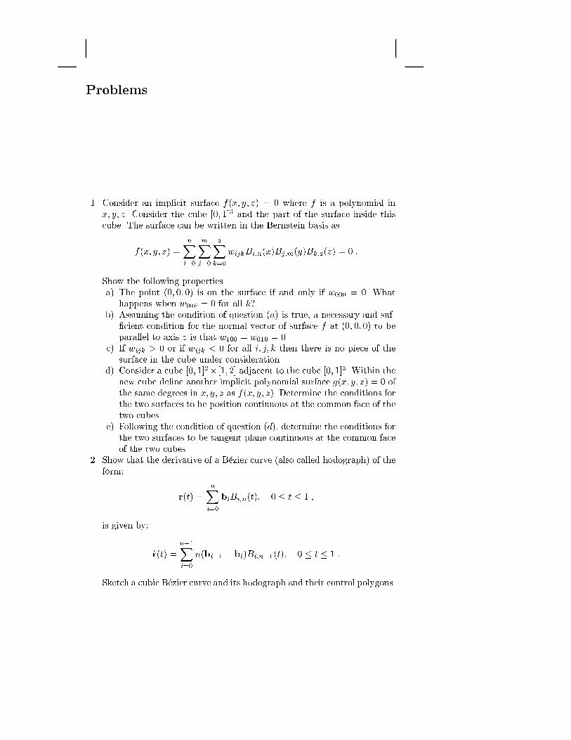
Problems
1. Consider an implicit surface f(x; y; z) = 0 where f is a polynomial inx; y; z. Consider the cube [0; 1]3 and the part of the surface inside thiscube. The surface can be written in the Bernstein basis as
f(x; y; z) =
nXi=0
mXj=0
qXk=0
wijkBi;n(x)Bj;m(y)Bk;q(z) = 0 :
Show the following properties.a) The point (0; 0; 0) is on the surface if and only if w000 = 0. What
happens when w00k = 0 for all k?b) Assuming the condition of question (a) is true, a necessary and suf-
�cient condition for the normal vector of surface f at (0; 0; 0) to beparallel to axis z is that w100 = w010 = 0.
c) If wijk > 0 or if wijk < 0 for all i; j; k then there is no piece of thesurface in the cube under consideration.
d) Consider a cube [0; 1]2� [1; 2] adjacent to the cube [0; 1]3. Within thenew cube de�ne another implicit polynomial surface g(x; y; z) = 0 ofthe same degrees in x; y; z as f(x; y; z). Determine the conditions forthe two surfaces to be position continuous at the common face of thetwo cubes.
e) Following the condition of question (d), determine the conditions forthe two surfaces to be tangent plane continuous at the common faceof the two cubes.
2. Show that the derivative of a B�ezier curve (also called hodograph) of theform:
r(t) =
nXi=0
biBi;n(t); 0 � t � 1 ;
is given by:
_r(t) =n�1Xi=0
n(bi+1 � bi)Bi;n�1(t); 0 � t � 1 :
Sketch a cubic B�ezier curve and its hodograph and their control polygons.

370 Problems
3. The degree elevation formula for B�ezier curves of degree n is given (1.54).Describe a process for approximating a B�ezier curve of degree n with aB�ezier curve of degree n� 1 using (1.54) reversely.
4. Show how an explicit polynomial curve y = y(x), where a � x � b can beconverted into a B�ezier curve. Provide the control points of the resultingB�ezier curve. And show how an explicit polynomial surface z = f(x,y),where a � x � b and c � y � d can be converted into a B�ezier patch andprovide its control points. Extend this to an explicit B-spline patch andprovide its control points.
5. Given a planar B-spline curve in the xy plane with a non-uniform knotvector, the control polygon of which is symmetric with respect to they-axis, �nd if the curve is also symmetric about the y-axis.
6. What kind of curve is the result of a perspective projection of an integralB-spline curve?
7. Consider the arc of the hyperbola y = 1x for 1 � x � 2 and re-
volve it around the axis y = 0 by �2 , to obtain the quadrant of a sur-
face of revolution, within the �rst octant of the xyz coordinate system(x � 0; y � 0; z � 0). Express the resulting patch in terms of a rationalbiquadratic parametric B�ezier surface patch.
8. Examine what happens to a cubic B-spline curve in which two, three, orfour consecutive vertices, of its control polygon are coincident.
9. Examine what might happen when a rational B-spline curve given by(1.87) or a rational B�ezier curve given by (1.88) has weights some ofwhich are positive and some are negative. Examine the validity of theproperties of the rational B-spline or rational B�ezier curves in such cases.
10. Make plots of the B-spline basis functions of the following order n (degree= n� 1) and knot vector T:� n = 4, T = (0; 0; 0; 0; 1; 1; 1; 1)� n = 4, T = (0; 0; 0; 0; 1; 3; 3; 3; 3)� n = 4, T = (0; 0; 0; 0; 2; 2; 4; 4; 4; 4)� n = 4, T = (0; 0; 0; 0; 1; 1; 1; 3; 3; 3; 3)� n = 4, T = (0; 0; 0; 0; 1; 2; 3; 4; 6; 7; 7; 7; 7)� n = 3, T = (0; 0; 0; 2; 4; 6; 6; 6)� n = 2, T = (0; 0; 1; 2; 2)
11. Given a list of Cartesian points in 3-D space which represent a non-periodic curve, construct a cubic B�ezier curve using least squares ap-proximation of the points. Also, construct a cubic B-spline curve withnon-uniform knots using least squares approximation of these points. Auser should be able to access your program with an arbitrary numberof points and coordinates of points. Include a simple visualization of theresults.
12. A cubic planar B�ezier curve:
r(t) =
3Xi=0
biBi;3(t) 0 � t � 1 ;
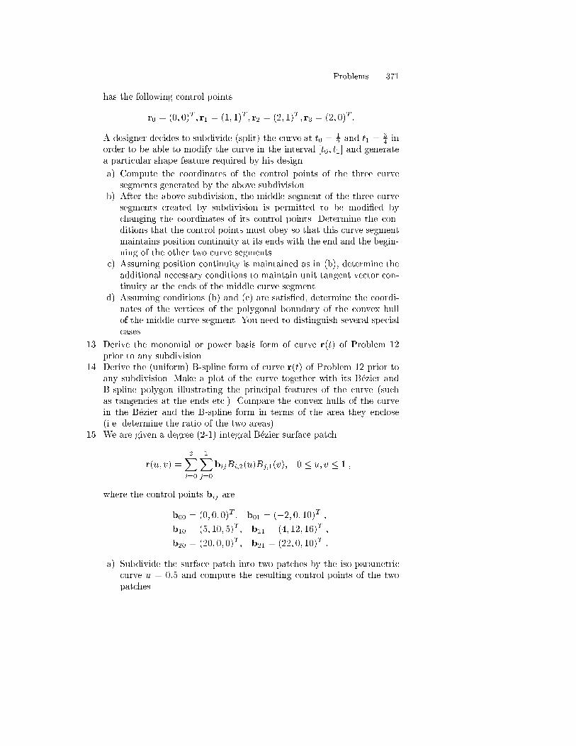
Problems 371
has the following control points
r0 = (0; 0)T ; r1 = (1; 1)T ; r2 = (2; 1)T ; r3 = (2; 0)T :
A designer decides to subdivide (split) the curve at t0 =12 and t1 =
34 in
order to be able to modify the curve in the interval [t0; t1] and generatea particular shape feature required by his design.
a) Compute the coordinates of the control points of the three curvesegments generated by the above subdivision.
b) After the above subdivision, the middle segment of the three curvesegments created by subdivision is permitted to be modi�ed bychanging the coordinates of its control points. Determine the con-ditions that the control points must obey so that this curve segmentmaintains position continuity at its ends with the end and the begin-ning of the other two curve segments.
c) Assuming position continuity is maintained as in (b), determine theadditional necessary conditions to maintain unit tangent vector con-tinuity at the ends of the middle curve segment.
d) Assuming conditions (b) and (c) are satis�ed, determine the coordi-nates of the vertices of the polygonal boundary of the convex hullof the middle curve segment. You need to distinguish several specialcases.
13. Derive the monomial or power basis form of curve r(t) of Problem 12prior to any subdivision.
14. Derive the (uniform) B-spline form of curve r(t) of Problem 12 prior toany subdivision. Make a plot of the curve together with its B�ezier andB-spline polygon illustrating the principal features of the curve (suchas tangencies at the ends etc.). Compare the convex hulls of the curvein the B�ezier and the B-spline form in terms of the area they enclose(i.e. determine the ratio of the two areas).
15. We are given a degree (2-1) integral B�ezier surface patch
r(u; v) =
2Xi=0
1Xj=0
bijBi;2(u)Bj;1(v); 0 � u; v � 1 ;
where the control points bij are
b00 = (0; 0; 0)T ; b01 = (�2; 0; 10)T ;b10 = (5; 10; 5)T ; b11 = (4; 12; 16)T ;
b20 = (20; 0; 0)T ; b21 = (22; 0; 10)T :
a) Subdivide the surface patch into two patches by the iso-parametriccurve u = 0:5 and compute the resulting control points of the twopatches.

372 Problems
b) Consider the boundary curve of the patch q(u) = r(u; 0). Provide atight upper bound for the maximum deviation of the curve q(u) inthe interval k
n � u � k+1n to the straight line passing via q( kn ) and
q(k+1n ) for a �xed value of k(2 0; 1; � � � ; n � 1), where n is a �xed
positive integer.c) i. Show that the given integral B�ezier surface is a developable sur-
face.ii. Are there any umbilics on this patch?
16. Consider a curve u = t, v = t2 for 0 � t � 1 on a hyperbolic paraboloidr(u; v) = (u; v; uv)T where 0 � u; v � 1.a) Compute the arc length of the curve on the hyperbolic paraboloid
for 0 � t � 1.b) Compute the area of a region of the hyperbolic paraboloid bounded
by positive v axis, v = 1 and a parabola v = u2.17. Consider a torus parametrized as follows:
r(u; v) = ((R + a cos u)cos v; (R+ a cos u)sin v; a sin u)T ;
where 0 � u � 2�; 0 � v � 2� and R > a. Derive appropriate formu-lae for the Gauss, mean and principal curvatures. Sketch the torus andsubdivide it into hyperbolic, parabolic and elliptic regions. In a follow-upsketch illustrate the lines of curvature of the torus. Explain the abovesubdivision and sketches.
18. Show that the curvature of a planar curve is independent of the parametriza-tion. Namely, if
r(t) = (x(t); y(t))T ;
is the curve, then a change of variables
t = w(u) with _w(u) 6= 0 ;
does not a�ect the curvature.19. Write a one-dimensional nonlinear polynomial solver based on Projected
Polyhedron algorithm. Use the solver to compute the roots of the degree20 Wilkinson polynomial with di�erent tolerances and discuss robustnessissues.
20. Convert an explicit curve y = x3 (�a � x � a) into a cubic B�ezier curve.21. Convert the following height function
z = h(x; y) = 7:2x3y3 � 25:2x3y2 + 18x3y � 10:8x2y3 + 37:8x2y2 � 27x2y
+ 3:6xy3 � 12:6xy2 + 9xy; 0 � x; y � 1 ;
into a bicubic B�ezier patch.22. Compute the characteristic points of the following curve
f(u; v) = (x2 + y2 � 2x)2 � (x2 + y2) = 0; [x; y] 2 [�4; 4]2 ;and trace it.

Problems 373
23. Consider the intersection curve of (11.135) with the plane 15x � 55z +110 = 0.a) Derive an implicit equation f(u; v) = 0 for this intersection curve
in the parameter space u; v. Find the characteristic points of thiscurve, (border, turning, and singular points).
b) Express this intersection curve as an explicit curve in the u; v pa-rameter space. Indicate the resulting type and degree of this curve.Sketch this curve in the parameter space u; v.
c) Prove that the above intersection curve is a planar rational B�ezierparametric curve of degree 4 in 3D space. Indicate how you wouldcompute its control points (but do not carry out the algebra).
24. Consider the following curves:
f(x; y) = � 64y4 + 128y3 � 96x2y2 + 140xy2 � 139y2 + 96x2y � 140xy
+ 75y � 96x4 + 276x3 � 313x2 + 165x� 36 = 0 ;
and
r(t) = (x(t); y(t))T =
3Xi=0
biBi;4(t) ;
where Bi;4(t) denotes the ith cubic Bernstein polynomial and r0 =(0:5; 0:5)T , b1 = (0:7; 0:6)T , b2 = (0:95; 0:1)T , b3 = (0:55; 0:25)T .
a) Compute all turning and singular points of f(x; y) to the highestpossible accuracy, as well as the tangent lines at all these points.
b) Using the results of a as a guide, sketch f(x; y). Clearly indicate theturning and singular points on your sketch.
c) Compute the intersections of the two curves given above to the high-est possible accuracy. In addition to giving the Cartesian coordinatesof the intersection points, also include the parameter values of thepoints and their multiplicity.
25. Write a program which determines all intersections of two integral planarB�ezier curves of arbitrary degrees m and n as accurately as possible,given the control points of the two curves. Your program should reportthe parametric values of the intersection points as well as the Cartesiancoordinates. Give four examples to show how your program works.
26. The following three planar curves are given by:
1) Implicit curve, f(x; y) = x3 + y3 � 3xy = 0 ;
2) Cubic B�ezier curve r(t) = (x(t); y(t))T =P3
i=0 riBi;4(t) where 0 �t � 1 and with r0 = (0; 0)T , r1 = (0; 2)T , r2 = (2; 0)T , r3 = (0;�2)T ;
3) Cubic B�ezier curve q(u) = (x(t); y(t))T =P3
i=0 qiBi;4(u) where 0 �t � 1 and with q0 = (�2;�2)T , q1 = (�2; 1)T , q2 = (4; 1)T , q3 =(0;�1)T :

374 Problems
a) Compute the characteristic points of the �rst curve in the rectangle[-5,5]�[-5,5] and trace it within the same rectangle.
b) Compute the intersections of the �rst and second curves, and thesecond the third curves to the highest possible accuracy, and identifytheir multiplicity.
c) Obtain a parametrization of the �rst curve in terms of rational poly-nomials using the transform y = xt. Illustrate x(t) and y(t) for allreal t. Is this a good parametrization for computer implementation(e.g. tracing of the curve) near x = y = 0? Can you suggest betterparametrizations for the curve piece in the �rst quadrant.
27. Compute the intersection curve between the bicubic B�ezier patch of Prob-lem 21 and a plane x�y+z = 0. Evaluate the curvature of the intersectioncurve at u = v = 0:5.
28. Give the implicit polynomial equation of a torus whose section cir-cle has radius 2, and whose center circle has radius 4 using the im-plicitization of a surface of revolution. Assume the torus is situatedso that it is centered at the origin and the center circle lies entirelyin the (x; y)-plane. Using the implicit equation, compute all intersec-tions of the torus with the cubic B�ezier curve having control pointsr0 = (0; 6; 0)T ; r1 = (�5; 2;�0:5)T ; r2 = (2;�3; 0:5)T ; r3 = (6; 0; 0)T .Give both the Cartesian coordinates of the intersection points and theirassociated parameter values on the B�ezier curve. Indicate which methodyou used to solve this problem, and give all answers to at least 5 signi�-cant digits.
29. Compute the minimum distance between a point (0.8, 0.7, 0.2) and aniso-parametric line v = 0:8 of the bicubic B�ezier patch of Problem 21.Also compute the minimum distance between the point and the bicubicpatch.
30. Consider two planar B�ezier curves which are cubic and quadric with con-trol points: (0,0), (1, 1), (2,1), (3,0) and (0,1), ( 34 , -1), (
64 , 5), (
94 , -1),
(3,0), respectively. Compute all stationary points of their squared dis-tance function and classify them appropriately into extrema etc. Identifythe corresponding Euclidean distances, �nd the points of intersection ofthe two curves and the angles between the tangents of the two curves atthe intersection points.
31. Consider an ellipsoid of revolution given by (3.81) with a=b=1, c=2 anda cubic planar B�ezier curve with control points (0,1, -2), (0,0, -1), (0,0,1),(0,1,2) on the x=0 plane. Compute the stationary points of the squareddistance function between the ellipsoid and the curve, classify them intoextrema etc. Identify the corresponding Euclidean distances, �nd thepoints of intersection and the angles between the surface normals andthe B�ezier curve tangents at the intersection points.
32. Find the stationary points of the squared distance function between theplane z=0 and the wave-like B�ezier surface patch of the example in Sect.

Problems 375
8.5.4 and Fig. 8.11. Classify the points into extrema etc., identify thecorresponding distances, and determine the intersections of the two sur-faces. Compare the locations of the above extrema with the locations ofthe various curvature extrema in Sect. 8.5.4.
33. Consider a torus generated by revolving the circle (x � 2)2 + y2 � 1 = 0around the y axis by a full revolution. Determine the stationary points ofthe squared distance function between this torus and a) a plane x = �3,b) a plane y = 2, c) a plane y = 1, d) a sphere with center the origin andradius r = 1
2 and e) a sphere with center the origin and radius r = 4.34. Consider a biquadratic Bezier surface patch whose boundary eight control
points are coplanar so that the boundary curves form a square [0; 1]2 onthe xy plane. The boundary non-corner control points are in the middleof the corresponding boundary edges. The central control point of thepatch has coordinates ( 12 ,
12 , h) where h = 0. Determine the surface unit
normal vector at the four corners, and at the center, and the extrema ofthe Gauss, mean and principal curvatures and any umbilics as a functionof h and illustrate this for h = 1
10 , 1, 10, 100. Sketch the lines of curvatureof the surface patch for these four values of h.
35. Find the range of mean curvature of a hyperbolic paraboloid r(u; v) =(u; v; uv)T , (u; v) 2 [0; 1]2 (bilinear surface), and plot four levels of con-tour lines of mean curvature in the uv-parameter space.
36. Given an implicit surface f(x; y; z) = 0, formulate the problem of tracingthe lines of curvature and develop an algorithm to do this. Test the re-sulting implementation for various standard algebraic surfaces (quadrics,torii, cyclides).
37. Given an implicit algebraic surface f(x; y; z) = 0, formulate the problemof locating the umbilics of the surface (within a given rectangular boxwith faces parallel to the coordinate planes).
38. Consider an ellipsoid x2
a2 +y2
b2 + z2
c2 = 1 where a � b � c.a) Show that umbilics are located at
��aq
b2�a2c2�a2 ; 0; �c
qc2�b2c2�a2
�.
b) Show that the patterns of the four umbilics are of the lemon type.39. Consider a degree (3-1) integral B�ezier surface
r(u; v) =
3Xi=0
1Xj=0
bijBi;3(u)Bj;1(v); 0 � u; v � 1 ;
where
b00=(0; 0; 0)T , b01=(0:5; 0; 2)
T ,b10=(1:8; 3; 0)
T , b11=(1:895; 2:325; 2)T ,
b20=(3:3;�2; 1:5)T , b21=(3:0575;�1:55; 3:1625)T ,b30=(4; 0; 0)
T , b31=(3:6; 0; 2)T .
a) Show that the B�ezier surface is a developable surface.

376 Problems
b) Is there an in ection line? If so, �nd the u parameter which containsthe in ection.
40. Derive di�erential equations for geodesics (10.17) - (10.20) on a paramet-ric surface using Euler's equation (10.24).
41. Write a program which solves di�erential equations for geodesics (10.17)- (10.20) as a boundary value problem using a shooting method on aparametric surface.
42. For the surface patch of Problem 34 compute the geodesics between twodiagonally opposite corners for various values of h. How do these geodesicschange as h changes from 0 to large positive values, e.g. in the interval[0,100]. What do you expect in the limit h tends to plus in�nity?
43. Let r(s) be a planar, closed and convex curve ( e.g. a circle, an ellipse,etc.) where the arc length s varies in the range [0; l] so that the length ofthe curve is l. Let
r(s) = r(s) + dn(s) ;
be its o�set curve, where d is a positive distance and n(s) is the unitnormal vector of the curve r de�ned by t � ez (see convention (b) of(2.24) in Table 3.2.)
a) Show that the total length of the curve r(s) exceeds the total lengthof the curve r(s) by 2�d.
b) Show that the area enclosed between the two curves is given by A =d(l + �d).
c) Show that the curvatures of the two curves are related by
� =�
1 + d�;
where � is the curvature of r(s) and � is the curvature of the o�setcurve r(s).
d) Verify your results for questions a to c for a circle of radius R.
44. This problem focuses on the identi�cation of cusps, extraordinary pointsand self-intersections of o�sets of planar curves (use convention (b) of(2.24) for the normal vector in Table 3.2.). Consider the ellipse x2+4y2 =1 or x = cos�; y = 1
2sin� and its o�set at \distance" d, where d is anyreal number.
a) Determine all the values of � for which there can be an extraordinarypoint on some o�set of the ellipse and the values of d at such points.Sketch the o�sets at all such values of d.
b) For what range of values of d, are o�sets of the ellipse regular curves?Sketch a few such o�set curves.
c) Determine a speci�c o�set of the ellipse which includes several cuspsand self-intersections but no extraordinary points. In�nite such casesexist. Give the parameter values and coordinates of these cusps andself-intersections. (Hint: Notice that self-intersections are on the axesof symmetry of the ellipse.)

Problems 377
45. Consider the planar cubic integral Bezier curve r(t) with control points(0; 0); (0; 1); (2; 1), and (2;�1). The o�set r of r at a distance d is givenby
r(t) = r(t) + dn(t) ;
where n(t) denotes the normal to r at the point r(t) de�ned by t � ez(see convention (b) of (2.24) in Table 3.2). Here r is called the progenitorof r.
a) For values of d between 0 and some critical value dc, the o�set curveresembles its progenitor. At d = dc, however, the o�set exhibits acusp at a parameter value tc because _r(tc) = 0. Compute the valuesof dc and tc.
b) Sketch the progenitor curve, and two o�set curves, one at a distanceof dc and one at a distance of around 2dc.
46. The evolute of a planar curve is the curve of its center of curvature.Show that cusps and extraordinary points of the o�set lie on the evolute.Illustrate the concept by examining the superbola x = t, y = t4, �2 �t � 2. Draw the curve, its evolute, and several o�sets with o�set distance,d = �0:25, d ' 0:4648, d = �0:8, d = �1, d = �1:25 (all on the concaveside).
47. Consider a pocket to be machined, bounded by the following four curves:1) x = t, y = t4, �2 � t � 2,2) y = 16,3) Two circular blends of the �rst and second curves with radius, r = 0:25.a) Construct an approximation of the medial axis (skeleton) of the
pocket in terms of a set of linear spline curves. The skeleton is theset of points inside the shape with two or more nearest points on theboundary of the shape. The skeleton branches potentially start at thecurvature centers corresponding to points of maximum curvature ofthe boundary. Next, you may specify the skeleton by writing di�er-ential equations relating the tangent vector of the skeleton to knownfunctions. For simplicity, write these equations for the speci�c ex-ample. Integrate these di�erential equations using the Runge-Kuttamethod.
b) Assuming you have cylindrical cutters with radii: 0.25, 0.5, 0.75, � � �,2, describe an e�cient method to accurately machine the pocket.
48. Write a program which approximates an o�set curve of a planar rationalcurve following the algorithm developed by Tiller and Hanson [420].
49. Give the implicit polynomial equation of a torus with axis in the direction(0,0,1), center circle radius R and section circle radius a where R > a.What is the equation of the o�set of this torus by �h, h > 0.
50. A pipe surface or canal surface of spheres of constant radius is de�nedas the envelope of a family of spheres of constant radius r whose centersdescribe a smooth curve, c(t) known as the spine. Let f(p; t) = jp �c(t)j2 � r2, where p = (x; y; z)

378 Problems
a) Show that the canal surface has an implicit equation g(p) = 0 whichresults from eliminating t from the two equations f = 0 and ft = 0.
b) Obtain the implicit equation of a torus by using the approach of parta).
c) Show that canal surfaces can be obtained as generalized cylinders bysweeping a circular cross-section along the spine.
51. In this problem we consider developing a blending surface between theplane z = 0 and the right circular cylinder x2 + y2 = 1; 0 � z � 2.Because the cylinder is a surface of revolution, we will, for simplicity,consider the cross-section of the objects obtained by setting y = 0. Ourproblem is to develop a smooth surface between the cylinder and theplane by creating a cross-section curve starting at height 1 on the cylinderand terminating on the plane 2 units away from the origin.
a) As a �rst e�ort, consider using a quadratic Bezier curve (i.e. aparabola) as a blend cross-section. The curve should have the start-ing and ending points as indicated above, and to ensure a smoothblend, the tangent to the curve at the start (end) point should havethe same direction as the tangent to the cylinder (plane). Give thecontrol points of this curve.
b) Using the results of part a), express the blending surface (i.e. thesurface of revolution characterized by the cross section obtained ina) as rational B-spline (NURBS) surface.
c) Now suppose we want a cubic Bezier curve as the cross-section ofour blending surface. Give the control points of a cubic Bezier curvewhich generates a \good" blend. To be \good", the curve not onlyhas to satisfy the boundary conditions indicated in part a, but alsothe area under the curve should be between 0:2 and 0:3.
d) Now suppose we want to maintain curvature continuity at the blend-ing surface linkage curves in addition to position and tangent planecontinuity. Determine a su�ciently high degree Bezier curve crosssection to accomplish this.

A. Color Plates
Color Plate A.1. Isophotes for surface of Fig. 8.1
Color Plate A.2. Re ection lines for surface of Fig. 8.1

380 A. Color Plates
Color Plate A.3. Gaussian curvature color map of surface in Fig. 8.11 (adaptedfrom [254])
Color Plate A.4. Mean curvature color map of surface in Fig. 8.11 (adapted from[254])

A. Color Plates 381
Color Plate A.5. Maximum principal curvature color map of surface in Fig. 8.11(adapted from [254])
Color Plate A.6. Minimum principal curvature color map of surface in Fig. 8.11(adapted from [254])

382 A. Color Plates
(a) (b) (c)
Color Plate A.7. (a) Star pattern (extracted from lower left umbilic of Fig. 9.6),(b) monstar pattern (extracted from center umbilic of Fig. 9.6). (c) lemon pattern(extracted from lower umbilic of Fig. 9.1) (adapted from [256])
x
y
z
Color Plate A.8. Minimal geodesic paths on the generalized cylinder between twopoints of two circular edges (adapted from [246])

References
1. K. Abdel-Malek and H.-J. Yeh. On the determination of starting points forparametric surface intersections. Computer-Aided Design, 29(1):21{35, January1997.
2. S. S. Abhyankar. Algebraic Geometry for Scientists and Engineers. AmericanMathematical Society, Providence, RI, 1990.
3. S. L. Abrams, L. Bardis, C. Chryssostomidis, N. M. Patrikalakis, S. T. Tuohy,F.-E. Wolter, and J. Zhou. The geometric modeling and interrogation systemPraxiteles. Journal of Ship Production, 11(2):117{132, May 1995.
4. S. L. Abrams, W. Cho, C.-Y. Hu, T. Maekawa, N. M. Patrikalakis, E. C. Sher-brooke, and X. Ye. E�cient and reliable methods for rounded-interval arith-metic. Computer-Aided Design, 30(8):657{665, July 1998.
5. P. G. Alourdas. Shape Creation, Interrogation and Fairing Using B-Splines.Engineer's thesis, Massachusetts Institute of Technology, Department of OceanEngineering, Cambridge, Massachusetts, 1989.
6. L.-E. Andersson, T. J. Peters, and N. F. Stewart. Sel�ntersection of compositecurves and surfaces. Computer Aided Geometric Design, 15(5):507{527, May1998.
7. R. K. E. Andersson. Surfaces with prescribed curvature I. Computer AidedGeometric Design, 10(5):431{452, October 1993.
8. E. V. Anoshkina, A. G. Belyaev, and T. L. Kunii. Detection of ridges andravines based on caustic singularities. International Journal of Shape Modeling,1(1):13{22, 1994.
9. E. V. Anoshkina, A. G. Belyaev, O. G. Okunev, and T. L. Kunii. Ridgesand ravines: A singularity approach. International Journal of Shape Modeling,1(1):1{11, 1994.
10. ANSI/IEEE Std 754{1985. IEEE Standard for Binary Floating{Point Arith-metic. IEEE, New York, 1985. Reprinted inACM SIGPLAN Notices, 22(2):9-25,February 1987.
11. S. Aomura and T. Uehara. Self-intersection of an o�set surface. Computer-Aided Design, 22(7):417{422, September 1990.
12. C. G. Armstrong, T. K. H. Tam, D. J. Robinson, R. M. McKeag, and M. A.Price. Automatic generation of well structured meshes using medial axis andsurface subdivision. In G. A. Gabriele, editor, Proceedings of the 17th ASMEDesign Automation Conference: Advances in Design Automation, Vol. 2, pages139{146, Miami, FL, September 1991. New York: ASME.
13. G. Aumann. Interpolation with developable B�ezier patches. Computer AidedGeometric Design, 8(5):409{420, November 1991.
14. F. Aurenhammer. Voronoi diagrams | a survey of fundamental geometric datastructure. ACM Computing Surveys, 23(3):345{405, September 1991.
15. W. Auzinger and H. J. Stetter. An elimination algorithm for the computationof zeros of a system of multivariate polynomial equations. In R. P. Agarwal,
384 References
Y. M. Chow, and S. J. Wilson, editors, Numerical Mathematics, Singapore,1988, International Series of Numerical Mathematics,Volume 86, pages 11{30.Birkh�auser Verlag, Boston Basel Berlin, 1988.
16. C. Bajaj, J. Chen, and G. Xu. Modeling with cubic A-patches. ACM Trans-actions on Graphics, 14(2):103{133, April 1995.
17. C. L. Bajaj, C. M. Ho�mann, J. E. Hopcroft, and R. E. Lynch. Tracing sur-face intersections. Computer Aided Geometric Design, 5(4):285{307, November1988.
18. R. E. Barnhill, G. Farin, L. Fayard, and H. Hagen. Twists, curvatures andsurface interrogation. Computer-Aided Design, 20(6):341{346, July 1988.
19. R. E. Barnhill, G. Farin, M. Jordan, and B. R. Piper. Surface/surface inter-section. Computer Aided Geometric Design, 4(1-2):3{16, July 1987.
20. R. E. Barnhill and S. N. Kersey. A marching method for parametric surface /surface intersection. Computer Aided Geometric Design, 7(1-4):257{280, June1990.
21. R. C. Beach. An Introduction to the Curves and Surfaces of Computer-AidedDesign. Van Nostrand Reinhold, New York, 1991.
22. J. M. Beck, R. T. Farouki, and J. K. Hinds. Surface analysis methods. IEEEComputer Graphics and Applications, 6(12):18{36, December 1986.
23. K.-P. Beier and Y. Chen. Highlight{line algorithm for realtime surface-qualityassessment. Computer-Aided Design, 26(4):268{277, April 1994.
24. M. V. Berry and J. H. Hannay. Umbilic points on Gaussian random surfaces.Journal of Physics A., 10(11):1809{1821, 1977.
25. D. Blackmore, M. C. Leu, and L. P. Wang. Sweep-envelope di�erential equationalgorithm and its application to NC machining veri�cation. Computer-AidedDesign, 29(9):629{637, September 1997.
26. W. Blaschke. Kreis und Kugel. Walter de Gruyter and Co., Berlin, 1956.27. C. Bliek. Computer Methods for Design Automation. PhD thesis, Massachusetts
Institute of Technology, Cambridge, MA, July 1992.28. G. A. Bliss. The geodesic lines on the anchor ring. Annals of Mathematics,
4:1{21, October 1902.29. H. Blum. Biological shape and visual science (part I). Journal of Theoretical
Biology, 38:205{287, 1973.30. H. Blum. A transformation for extracting new descriptors of shape. Models for
the Perception of Speech and Visual Form, pages 362{381, ed: Weinant Wathen-Dunn MIT Press, 1967.
31. H. Blum and R. N. Nagel. Shape description using weighted symmetric axisfeatures. Pattern Recognition, 10(3):167{180, 1978.
32. R. M. C. Bodduluri and B. Ravani. Design of developable surfaces using dualitybetween plane and point geometries. Computer-Aided Design, 25(10):621{632,October 1993.
33. W. Boehm. Cubic b-spline curves and surfaces in computer aided geometricdesign. Computing, 19:29{34, 1977.
34. W. Boehm. Inserting new knots into B-spline curves. Computer-Aided Design,12(4):199{201, July 1980.
35. W. Boehm. Subdividing multivariate splines. Computer-Aided Design,15(6):345{352, November 1983.
36. F. L. Bookstein. The line skeleton. Computer Graphics and Image Processing,11:123{137, 1979.
37. M. Brady, J. Ponce, A. Yuille, and H. Asada. Describing surfaces. ComputerVision, Graphics and Image Processing, 32(1):1{28, October 1985.

References 385
38. J. W. Brandt. Theory and Application of the Skeleton Representation of Con-tinuous Shapes. PhD thesis, University of California, Davis, CA, December1991.
39. J. W. Brandt. Describing a solid with the three-dimensional skeleton. In J. D.Warren, editor, Proceedings of The International Society for Optical Engineer-ing, Volume 1830, Curves and Surfaces in Computer Vision and Graphics III,pages 258{269. SPIE, Boston, Massachusetts, 1992.
40. J. W. Brandt. Convergence and continuity criteria for discrete approximationsof the continuous planar skeleton. CVGIP: Image Understanding, 59(1):116{124, January 1994.
41. J. W. Brandt and V. R. Algazi. Continuous skeleton computation by Voronoidiagram. CVGIP: Image Understanding, 55(3):329{338, May 1992.
42. J. W. Brandt and V. R. Algazi. Lossy encoding of document images with thecontinuous skeleton. In P. Maragos, editor, Visual Communications and ImageProcessing '92, SPIE 1818, pages 663{673, 1992.
43. J. W. Brandt, A. K. Jain, and V. R. Algazi. Medial axis representation andencoding of scanned documents. Journal of Visual Communication and ImageRepresentation, 2(2):151{165, June 1991.
44. E. L. Brechner. General tool o�set curves and surfaces. In R. E. Barnhill, edi-tor, Geometry Processing for Design and Manufacturing, pages 101{121. SIAM,1992.
45. P. Brunet, A. Vinacua, M. Vivo, N. Pla, and A. Rodriguez. Surface fairing forship hull design application. Mathematical Engineering in Industry, 7(2):179{193, 1998.
46. B. Buchberger. Ein Algorithmus zum Au�nden der Basiselemente des Restk-lassenringes nach einem nulldimensionalen Polynomideal. PhD thesis, Univer-sity of Innsbruck, Innsbruck, Austria, 1965.
47. B. Buchberger. Gr�obner bases: An algorithmic method in polynomial idealtheory. In N. K. Bose, editor, Multidimensional Systems Theory: Progress,Directions and Open Problems in Multidimensional Systems, pages 184{232.Dordrecht, Holland: D. Reidel Publishing Company, 1985.
48. J. F. Canny. The Complexity of Robot Motion Planning. MIT Press, Cambridge,MA, 1988.
49. J. F. Canny and I. Z. Emiris. An e�cient algorithm for the sparse mixed re-sultant. In G. Cohen, T. Mora, and O. Moreno, editors, Proceedings of 10thInternational Symposium, Applied Algebra, Algebraic Algorithms and Error-Correcting Codes, pages 89{104. Springer-Verlag, 1993.
50. J. S. Chalfant. Analysis and Design of Developable Surfaces for Shipbuilding.Master's thesis, Massachusetts Institute of Technology, Department of OceanEngineering, Cambridge, Massachusetts, 1997.
51. B. W. W. Char, K. O. Geddes, G. H. Gonnet, B. L. Leong, M. B. Monagan, andS. M. Watt. First Leaves: A Tutorial Introduction to Maple V. Springer-Verlag,1992.
52. Y. J. Chen and B. Ravani. O�set surface generation and contouring incomputer-aided design. Journal of Mechanisms, Transmissions, and Automa-tion in Design, Transactions of the ASME, 109(3):133{142, March 1987.
53. K.-P. Cheng. Using plane vector �elds to obtain all the intersection curves oftwo general surfaces. In W. Strasser and H. Seidel, editors, Theory and Practiceof Geometric Modeling, pages 187{204. Springer-Verlag, New York, 1989.
54. C.-S. Chiang. The Euclidean Distance Transform. PhD thesis, Purdue Univer-sity, West Lafayette, IN, August 1992.
55. C. S. Chiang, C. M. Ho�mann, and R. E. Lynch. How to compute o�sets with-out self-intersection. In M. J. Silbermann and D. Tagare, editors, Proceedings of

386 References
The SPIE Conference on Curves and Surfaces in Computer Vision and Graph-ics II, Volume 1610, pages 76{87, Boston, Massachusetts, 1991. InternationalSociety for Optical Engineering.
56. H. Chiyokura. Solid Modelling with DesignBase. Addison-Wesley, Reading,MA, 1988.
57. W. Cho, T. Maekawa, N. M. Patrikalakis and J. Peraire, Topologically ReliableApproximation of Trimmed Polynomial Surface Patches. Graphical Models andImage Processing, 61(2):84{109, March 1999.
58. W. Cho, T. Maekawa, and N. M. Patrikalakis. Topologically reliable approxima-tion of composite B�ezier curves. Computer Aided Geometric Design, 13(6):497{520, August 1996.
59. B. K. Choi and R. Jerard. Sculptured Surface Machining - Theory and Appli-cations. Kluwer Academic Publishers, 1998.
60. B. K. Choi, C. S. Lee, and C. S. Jun. Compound surface modelling and ma-chining. Computer-Aided Design, 20(3):127{136, April 1988.
61. I. Choi and K. Lee. E�cient generation of re ection lines to evaluate car bodysurfaces. Mathematical Engineering in Industry, 7(2):233{250, 1998.
62. B. Cobb. Design of Sculptured Surfaces Using the B-spline Representation.PhD thesis, Computer Science Department, University of Utah, Salt Lake City,Utah, 1984.
63. E. Cohen, T. Lyche, and R. Riesenfeld. Discrete B-splines and subdivision tech-niques in computer-aided geometric design and computer graphics. ComputerGraphics and Image Processing, 14(2):87{111, October 1980.
64. G. E. Collins and R. Loos. Real zeros of polynomials. In B. Buchberger,G. E. Collins, and R. Loos, editors, Computer Algebra: Symbolic and AlgebraicComputation, pages 83{94. Springer-Verlag, Vienna, 1982.
65. S. Coquillart. Computing o�sets of B-spline curves. Computer-Aided Design,19(6):305{309, July/August 1987.
66. T. H. Cormen, C. E. Leiserson, and R. L. Rivest. Introduction to Algorithms.MIT Press, Cambridge, MA, 1990.
67. M. G. Cox. The numerical evaluation of B-splines. Journal of the Institute forMathematics Applications, 10:134{149, 1972.
68. T. Culver, J. Keyser, and D. Manocha. Accurate computation of the medialaxis of a polyhedron. In W. F. Bronsvoort and D. C. Anderson, editors, InProceedings of Fifth Symposium on Solid Modeling and Applications, Ann Arbor,Michigan, pages 179{190. NY: ACM, June 1999.
69. G. Dahlquist and �A. Bj�orck. Numerical Methods. Prentice-Hall, Inc., Engle-wood Cli�s, NJ, 1974.
70. P.-E. Danielsson. Euclidean distance mapping. Computer Graphics and ImageProcessing, 14:227{248, 1980.
71. G. Darboux. Le�cons sur la Th�eorie G�en�erale des Surfaces, Vol.4. Gauthier-Villars, Paris, 1896.
72. C. De Boor. On calculating with B-splines. Journal of Approximation Theory,6:50{62, 1972.
73. C. De Boor. A Practical Guide to Splines. Springer, New York, 1978.74. J. C. Dill. An application of color graphics to the display of surface curvature.
ACM Computer Graphics, 15(3):153{161, August 1981.75. Q. Ding and B. J. Davies. Surface Engineering Geometry for Computer-Aided
Design and Manufacture. Ellis Horwood, Chichester, UK, 1987.76. P. M. do Carmo. Di�erential Geometry of Curves and Surfaces. Prentice-Hall,
Inc., Englewood Cli�s, NJ, 1976.

References 387
77. T. Dokken. Finding intersections of B-spline represented geometries using re-cursive subdivision techniques. Computer Aided Geometric Design, 2(1-3):189{195, September 1985.
78. D. Dragomatz and S. Mann. A classi�ed bibliography of literature on NCmilling path generation. Computer-Aided Design, 29(3):239{247, 1997.
79. A. Dresden. A Solid Analytical Geometry and Determinants. Dover, New York,1964.
80. T. Du�. Interval arithmetic and recursive subdivision for implicit functionsand constructive solid geometry. ACM Computer Graphics, 26(2):131{138, July1992.
81. D. Dutta and C. M. Ho�mann. A geometric investigation of the skeleton ofCSG objects. In B. Ravani, editor, Proceedings of the 16th ASME Design Au-tomation Conference: Advances in Design Automation, Computer Aided andComputational Design, volume I, pages 67{75, Chicago, IL, September 1990.New York: ASME, 1990.
82. D. Dutta and C. M. Ho�mann. On the skeleton of simple CSG objects. Journalof Mechanical Design, ASME Transactions, 115(1):87{94, March 1993.
83. D. Dutta, R. R. Martin, and M. J. Pratt. Cyclides in surface and solid modeling.IEEE Computer Graphics and Applications, 13(1):53{59, January 1993.
84. H. Edelsbrunner and E. P. M�ucke. Three-dimensional alpha shapes. ACMTransactions on Graphics, 13(1):43{72, 1994.
85. G. Elber and E. Cohen. Error bounded variable distance o�set operator forfree form curves and surfaces. International Journal of Computational Geometryand Applications, 1(1):67{78, March 1991.
86. G. Elber and E. Cohen. O�set approximation improvement by control pointsperturbation. In T. Lyche and L. L. Schumaker, editors, Mathematical Meth-ods in Computer Aided Geometric Design II, pages 229{237. Academic Press,Boston, 1992.
87. G. Elber and E. Cohen. Second-order surface analysis using hybrid symbolicand numeric operators. ACM Transactions on Graphics, 12(2):160{178, April1993.
88. G. Elber, I.-K. Lee, and M. S. Kim. Comparing o�set curve approximationmethods. IEEE Computer Graphics and Applications, 17(3):62{71, May/June1997.
89. I. Z. Emiris. Sparse Elimination and Applications in Kinematics. PhD thesis,University of California at Berkeley, Berkeley, CA, 1994.
90. W. Enger. Interval Ray Tracing - A divide and conquer strategy for realisticcomputer graphics. The Visual Computer, 9(2):91{104, November 1992.
91. M. Etzion and A. Rappoport. Computing the Voronoi diagram of a 3-d poly-hedron by separate computation of its symbolic and geometric parts. In W. F.Bronsvoort and D. C. Anderson, editors, In Proceedings of Fifth Symposiumon Solid Modeling and Applications, Ann Arbor, Michigan, pages 167{178, NY:ACM, June 1999.
92. G. Farin. Curves and Surfaces for Computer Aided Geometric Design: A Prac-tical Guide. Academic Press, Boston, MA, 3rd edition, 1993.
93. R. T. Farouki. Exact o�set procedures for simple solids. Computer AidedGeometric Design, 2(4):257{279, 1985.
94. R. T. Farouki. The approximation of non-degenerate o�set surfaces. ComputerAided Geometric Design, 3(1):15{43, May 1986.
95. R. T. Farouki. The characterization of parametric surface sections. ComputerVision, Graphics and Image Processing, 33(2):209{236, February 1986.

388 References
96. R. T. Farouki. Graphical methods for surface di�erential geometry. In R. R.Martin, editor, The Mathematics of Surfaces II, pages 363{385. ClarendonPress, 1987.
97. R. T. Farouki. Hierarchical segmentations of algebraic curves and some ap-plications. In T. Lyche and L. L. Schumaker, editors, Mathematical Methodsin Computer Aided Geometric Design, pages 239{248. Academic Press, Boston,1989.
98. R. T. Farouki. On integrating lines of curvature. Computer Aided GeometricDesign, 15(2):187{192, February 1998.
99. R. T. Farouki and J. K. Johnstone. The bisector of a point and a plane para-metric curve. Computer Aided Geometric Design, 11(2):117{151, April 1994.
100. R. T. Farouki and J. K. Johnstone. Computing point/curve and curve/curvebisectors. In R. B. Fisher, editor, The Mathematics of Surfaces V, pages 327{354. Oxford University, Oxford, 1994.
101. R. T. Farouki and C. A. Ne�. Algebraic properties of plane o�set curves.Computer Aided Geometric Design, 7(1 - 4):101{127, 1990.
102. R. T. Farouki and C. A. Ne�. Analytic properties of plane o�set curves.Computer Aided Geometric Design, 7(1 - 4):83{99, 1990.
103. R. T. Farouki and C. A. Ne�. Hermite interpolation by Pythagorean hodo-graph quintics. Mathematics of Computation, 64(212):1589{1609, October 1995.
104. R. T. Farouki, C. A. Ne�, and M. A. O'Connor. Automatic parsing of degener-ate quadric-surface intersections. ACM Transactions on Graphics, 8(3):174{203,1989.
105. R. T. Farouki and V. T. Rajan. On the numerical condition of polynomials inBernstein form. Computer Aided Geometric Design, 4(3):191{216, November1987.
106. R. T. Farouki and V. T. Rajan. Algorithms for polynomials in Bernstein form.Computer Aided Geometric Design, 5(1):1{26, June 1988.
107. R. T. Farouki and V. T. Rajan. On the numerical condition of algebraiccurves and surfaces 1. implicit equations. Computer Aided Geometric Design,5:215{252, 1988.
108. R. T. Farouki and T. Sakkalis. Pythagorean hodographs. IBM Journal ofResearch and Development, 34(5):736{752, September 1990.
109. R. T. Farouki and T. Sakkalis. Real rational curves are not `unit speed'.Computer Aided Geometric Design, 8(2):151{157, May 1991.
110. R. T. Farouki and T. Sakkalis. Pythagorean-hodograph space curves. Ad-vances in Computational Mathematics, 2:41{46, 1994.
111. R. T. Farouki and T. W. Sederberg. Analysis of the o�set to a parabola.Computer Aided Geometric Design, 12(6):639{645, September 1995.
112. R. T. Farouki and S. Shah. Real-time CNC interpolators for Pythagorean-hodograph curves. Computer Aided Geometric Design, 13(7):583{600, October1996.
113. R. T. Farouki and R. Sverrisson. Approximation of rolling-ball blends for free-form parametric surfaces. Computer-Aided Design, 28(11):871{878, November1996.
114. R. T. Farouki, K. Tarabanis, J. U. Korein, J. S. Batchelder, and S. R. Abrams.O�set curves in layered manufacturing. Journal of Manufacturing Science andEngineering, Transactions of the ASME, 68(2):557{568, 1994.
115. J. C. Faugere, P. Gianni, D. Lazard, and T. Mora. E�cient computation ofzero-dimensional Gr�obner bases by change of ordering. Journal of SymbolicComputation, 16(4):329{344, 1993.
116. I. D. Faux and M. J. Pratt. Computational Geometry for Design and Manu-facture. Ellis Horwood, Chichester, England, 1981.

References 389
117. J. H. Ferziger. Numerical Methods for Engineering Applications. Wiley, 1981.118. J. D. Foley, A. Van Dam, S. K. Feiner, and J. F. Hughes. Computer Graphics:
Principles and Practice. Addison-Wesley, Reading, MA, 2nd edition, 1996.119. A. R. Forrest. Computational geometry. Proceedings of the Royal Society of
London A, 321:187{195, 1971.120. W. H. Frey and D. Bindschadler. Computer-aided design of a class of de-
velopable B�ezier surfaces. R&D Publication 8057, General Motors, September1993.
121. J. Gallier. Curves and Surfaces in Geometric Modeling: Theory and Algo-rithms. Morgan Kaufmann, San Francisco, CA, 1999.
122. J. Gallier. Geometric Methods and Applications: For Computer Science andEngineering. Springer-Verlag, New York, 2001.
123. C. B. Garcia and W. I. Zangwill. Global continuation methods for �nding allsolutions to polynomial systems of equations in n variables. In A. V. Fiaccoand K. O. Kortanek, editors, Extremal Methods and Systems Analysis, pages481{497. Springer-Verlag, New York, NY, 1980.
124. A. Geisow. Surface Interrogations. PhD thesis, School of Computing Studiesand Accountancy, University of East Anglia, Norwich NR47TJ, U. K., July1983.
125. S. M. Gelston and D. Dutta. Boundary surface recovery from skeleton curvesand surfaces. Computer Aided Geometric Design, 12(1):27{51, February 1995.
126. C. F. Gerald and P. O. Wheatley. Applied Numerical Analysis. Addison-Wesley, Reading, MA, 4th edition, 1990.
127. G. Glaeser, J. Wallner, and H. Pottmann. Collision-free 3-axis milling andselection of cutting tools. Computer-Aided Design, 31(3):225{232, March 1999.
128. D. Goldberg. What every computer scientist should know about oating{pointarithmetic. ACM Computing Surveys, 23(1):5{48, March 1991.
129. M. Golubitsky and V. Guillemin. Stable Mappings and their Singularities.Springer-Verlag, New York, 1973.
130. W. J. Gordon and R. F. Riesenfeld. B-spline curves and surfaces. In R. E.Barnhill and R. F. Riesenfeld, editors, Computer Aided Geometric Design, pages95{126. Academic Press, Inc., 1974.
131. T. A. Grandine. Computing zeroes of spline functions. Computer Aided Geo-metric Design, 6(2):129{136, May 1989.
132. T. A. Grandine. Geometry processing and numerical stability. In G. Farin,J. Hoschek, M. S. Kim, and D. Abma, editors, The Handbook of Computer AidedDesign. Elsevier, 2001.
133. T. A. Grandine and F. W. Klein. A new approach to the surface intersectionproblem. Computer Aided Geometric Design, 14(2):111{134, 1997.
134. J. A. Grant and G. D. Hitchins. An always convergent minimization techniquefor the solution of polynomial equations. Journal of Industrial and MathematicalApplications, 8:122{129, 1971.
135. J. A. Grant and G. D. Hitchins. Two algorithms for the solution of polynomialequations to limiting machine precision. The Computer Journal, 18(3), 1973.
136. A. Gray. Modern Di�erential Geometry of Curves and Surfaces. CRC Press,Boca Raton, 1993.
137. L. Guibas and J. Stol�. Primitives for the manipulation of general subdivisionsand the computation of Voronoi diagrams. ACM Transactions on Graphics,4(2):74{123, April 1985.
138. A. Z. Gurbuz and I. Zeid. O�setting operations via closed ball approximation.Computer-Aided Design, 27(11):805{810, November 1995.

390 References
139. H. N. Gursoy. Shape Interrogation by Medial Axis Transform for AutomatedAnalysis. PhD thesis, Massachusetts Institute of Technology, Cambridge, MA,November 1989.
140. H. N. Gursoy and N. M. Patrikalakis. Automated interrogation and adaptivesubdivision of shape using medial axis transform. Advances in EngineeringSoftware and Workstations, 13(5/6):287{302, September/November 1991.
141. H. N. Gursoy and N. M. Patrikalakis. An automated coarse and �ne surfacemesh generation scheme based on medial axis transform, part I: Algorithms.Engineering with Computers, 8(3):121{137, 1992.
142. H. N. Gursoy and N. M. Patrikalakis. An automated coarse and �ne surfacemesh generation scheme based on medial axis transform, part II: Implementa-tion. Engineering with Computers, 8(4):179{196, 1992.
143. C. Gutierrez and J. Sotomayor. Lines of curvature, umbilic points andCarath�eodory conjecture. Resenhas IME-UPS, 3(3):291{322, 1998.
144. J. Hadenfeld. Local energy fairing of B-spline surfaces. In M. D�hlen, T. Ly-che, and L. L. Schumaker, editors, Mathematical Methods for Curves and Sur-faces, pages 203{212. Vanderbilt University Press, 1995.
145. H. Hagen, S. Hahmann, and T. Schreiber. Visualization and computation ofcurvature behaviour of freeform curves and surfaces. Computer-Aided Design,27(7):545{552, July 1995.
146. H. Hagen, S. Hahmann, T. Schreiber, Y. Nakajima, B. W�ordenweber, andP. Hollemann-Grundstedt. Surface interrogation algorithms. IEEE ComputerGraphics and Applications, 12(5):53{60, September 1992.
147. G. D. Hager. Constraint solving methods and sensor-based decision mak-ing. In Proceedings of the 1992 IEEE International Conference on Robotics andAutomation, pages 1662{1667. IEEE, 1992.
148. S. Hahmann and S. Konz. Knot-removal surface fairing using search strategies.Computer-Aided Design, 30(12):923{930, February 1998.
149. D. G. Hakala, R. C. Hillyard, B. E. Nourse, and P. J. Malraison. Naturalquadrics in mechanical design. In Proceedings of the Autofact West 1, Anaheim,CA in November, 1980, pages 363{378, 1980.
150. B. Hamann and J. L. Chen. Data point selection for piecewise trilinear ap-proximation. Computer Aided Geometric Design, 11(5):477{489, October 1994.
151. R. W. Hamming. Numerical Methods for Scientists and Engineers. McGraw-Hill, New York, 1962.
152. H. Hancock. Theory of Maxima and Minima. Dover, New York, 1960.153. A. Hansen and F. Arbab. An algorithm for generating NC tool paths for arbi-
trarily shaped pockets with islands. ACM Transactions on Graphics, 11(2):152{182, 1992.
154. E. Hartmann. G2 interpolation and blending on surfaces. The Visual Com-puter, 12(4):181{192, 1996.
155. E. Hartmann. Numerical implicitization for intersection and Gn-continuousblending of surfaces. Computer Aided Geometric Design, 15(4):377{397, April1998.
156. R. N. Hawat and L. A. Piegl. Genetic algorithm approach to curve-curveintersection. Mathematical Engineering in Industry, 7(2):269{282, 1998.
157. M. Held. On the Computational Geometry of Pocket Machining. Springer-Verlag, Berlin, Germany, 1991.
158. P. Van Hentenryck, D. McAllester, and D. Kapur. Solving polynomial systemsusing a branch and prune approach. SIAM Journal on Numerical Analysis,34(2):797{827, April 1997.
159. P. Van Hentenryck, L. Michel, and Y. Deville. Numerica: A Modeling Languagefor Global Optimization. MIT Press, Cambride, MA, 1997.

References 391
160. H.-S. Heo, M.-S. Kim, and G. Elber. The intersection of two ruled surfaces.Computer-Aided Design, 31(1):33{50, January 1999.
161. T. Hermann. Geometrical criteria on the higher order smoothness of compositesurfaces. Computer Aided Geometric Design, 16(9):907{911, October 1999.
162. M. Higashi and K. Kaneko. Generation of high-quality curve and surface withsmoothly varying curvature. In D. A. Duce and P. Jancene, editors, Eurographics'88, pages 79{92, Nice, France, September 1988. North-Holland.
163. M. Higashi, T. Saitoh, Y. Watanabe, and Y. Watanabe. Analysis of aestheticfree-form surfaces by surface edges. In S. Y. Shin and T. L. Kunii, editors,Proceedings of the Third Paci�c Conference on Computer Graphics and Appli-cations, Paci�c Graphics '95, pages 294{305, Seoul, Korea, August 1995. WorldScienti�c.
164. M. Higashi, H. Tsutamori, and M. Hosaka. Generation of smooth surfacesby controlling curvature variation. Computer Graphics Forum, 15(3):187{196,September 1996.
165. D. Hilbert and S. Cohn-Vossen. Geometry and the Imagination. Chelsea, NewYork, 1952.
166. F. B. Hildebrand. Advanced Calculus for Applications. Prentice-Hall, Inc.,Englewood Cli�s, New Jersey, 1976.
167. C. M. Ho�mann. Geometric and Solid Modeling: An Introduction. MorganKaufmann Publishers, Inc., San Mateo, California, 1989.
168. C. M. Ho�mann. The problems of accuracy and robustness in geometriccomputation. Computer, 22(3):31{41, March 1989.
169. C. M. Ho�mann. A dimensionality paradigm for surface interrogations. Com-puter Aided Geometric Design, 7(6):517{532, November 1990.
170. C. M. Ho�mann. How to construct the skeleton of CSG objects. In A. Bowyerand J. Davenport, editors, Proceedings of the Fourth IMA Conference, TheMathematics of Surfaces, University of Bath, UK, September 1990, pages 421{438, New York, 1994. Oxford University Press.
171. C. M. Ho�mann and G. Vanecek. On alternate solid representations andtheir uses. Technical Report CSD-TR-91-019, Computer Sciences Department,Purdue University, March 1991.
172. D. H. Hoitsma. Surface curvature analysis. In M. J. Wozny et al., editors,IFIP TC5/WG5.2 Second Workshop on Geometric Modeling, pages 21{38, NewYork, 1988. IFIP, North Holland.
173. M. Hosaka. Modeling of Curves and Surfaces in CAD/CAM. Springer-Verlag,New York, 1991.
174. J. Hoschek. Spline approximation of o�set curves. Computer Aided GeometricDesign, 5(1):33{40, June 1988.
175. J. Hoschek and D. Lasser. Fundamentals of Computer Aided Geometric De-sign. A. K. Peters, Wellesley, MA, 1993. Translated by L. L. Schumaker.
176. J. Hoschek and N. Wissel. Optimal approximate conversion of spline curvesand spline approximation of o�set curves. Computer-Aided Design, 20(8):475{483, October 1988.
177. E. G. Houghton, R. F. Emnett, J. D. Factor, and C. L. Sabharwal. Implemen-tation of a divide-and-conquer method for intersection of parametric surfaces.Computer Aided Geometric Design, 2:173{183, 1985.
178. C. Y. Hu, T. Maekawa, N. M. Patrikalakis, and X. Ye. Robust interval algo-rithm for surface intersections. Computer-Aided Design, 29(9):617{627, Septem-ber 1997.
179. C. Y. Hu, T. Maekawa, E. C. Sherbrooke, and N. M. Patrikalakis. Robustinterval algorithm for curve intersections. Computer-Aided Design, 28(6/7):495{506, June/July 1996.
392 References
180. C. Y. Hu, N. M. Patrikalakis, and X. Ye. Robust interval solid modeling: PartI, Representations. Computer-Aided Design, 28(10):807{817, October 1996.
181. C. Y. Hu, N. M. Patrikalakis, and X. Ye. Robust interval solid modeling:Part II, Boundary evaluation. Computer-Aided Design, 28(10):819{830, October1996.
182. IGES/PDES Organization, U.S. Product Data Association, Fairfax, VA.Digital Representation for Communication of Product De�nition Data, USPRO/IPO-100, Initial Graphics Exchange Speci�cation (IGES) 5.2, November1993.
183. C. G. Jensen and D. C. Anderson. A review of numerically controled methodsfor �nish-sculptured-surface machining. IEE Transactions, 28:30{39, 1996.
184. R. B. Jerard, R. L. Drysdale, B. Schaudt, K. Hauck, and J. Magewick. Meth-ods for detecting errors in numerically controlled machining of sculptured sur-faces. IEEE Computer Graphics and Applications, 9(1):26{39, January 1989.
185. H. T. Jessop and F. C. Harris. Photoelasticity, Principles and Methods. NewYork: Dover Publications, 1950.
186. J. P. Jouanolou. Le formalisme du resultant. Advances in Mathematics,90(2):117{263, 1991.
187. J. T. Kajiya. Ray tracing parametric patches. ACM Computer Graphics,16(3):245{254, July 1982.
188. K. Kase, A. Makinouchi, T. Nakagawa, H. Suzuki, and F. Kimura. Shape errorevaluation method of free-form surfaces. Computer-Aided Design, 31(8):495{505, July 1999.
189. E. Kaufmann and R. Klass. Smoothing surfaces using re ection lines forfamilies of splines. Computer-Aided Design, 20(6):312{316, July 1988.
190. R. B. Kearfott. Interval Newton/generalized bisection when there are singu-larities near roots. Annals of Operations Research, 25:181{196, 1990.
191. R. B. Kearfott. Decomposition of arithmetic expressions to improve the be-havior of interval iteration for nonlinear systems. Computing, 47:169{191, 1991.
192. N. Kehtarnavaz and R. J. P. de Figueiredo. A 3-D contour segmentationscheme based on curvature and torsion. IEEE Transactions on Pattern Analysisand Machine Intelligence, 10(5):707{713, September 1988.
193. H. B. Keller. Numerical Methods for Two-Point Boundary Value Problems.Blaisdell, Waltham, MA, 1968.
194. B. W. Kernighan and D. M. Ritchie. The C Programming Language. Prentice-Hall, Englewood Cli�s, NJ, 2nd edition, 1988.
195. J. Keyser, T. Culver, D. Manocha, and S. Krishnan. E�cient and exact manip-ulation of algebraic points and curves. Computer-Aided Design, 32(11):649{662,September 2000.
196. K. I. Kim and K. Kim. A new machine strategy for sculptured surfaces usingo�set surface. International Journal of Production Research, 33(6):1683{1697,1995.
197. M.-S. Kim, E.-J. Park, and S.-B. Lim. Approximation of variable-radius o�-set curves and its application to B�ezier brush-stroke design. Computer-AidedDesign, 25(11):684{698, November 1993.
198. T. Kim and S. E. Sarma. Time-optimal paths covering a surface. In R. Cipollaand R. Martin, editors, The Mathematics of Surfaces IX, pages 126{143, Uni-versity of Cambridge, UK., September 2000. London: Springer.
199. R. Kimmel, A. Amir, and A. M. Bruckstein. Finding shortest paths on sur-faces using level sets propagation. IEEE Transactions on Pattern Analysis andMachine Intelligence, 17(6):635{640, June 1995.
200. R. Kimmel and A. M. Bruckstein. Shape o�sets via level sets. Computer-AidedDesign, 25(3):154{162, March 1993.
References 393
201. R. Klass. Correction of local surface irregularities using re ection lines.Computer-Aided Design, 12(2):73{76, March 1980.
202. R. Klass. An o�set spline approximation for plane cubic splines. Computer-Aided Design, 15(4):297{299, September 1983.
203. D. E. Knuth. The Art of Computer Programming, Vol. 2, SeminumericalAlgorithms. Addison-Wesley, Reading, Massachusetts, 1981. 2nd Edition.
204. J. J. Koenderink. Solid Shape. MIT Press, Cambridge, MA, 1990.205. E. Kreyszig. Di�erential Geometry. University of Toronto Press, Toronto,
1959.206. E. Kreyszig. Introduction to Di�erential Geometry and Riemannian Geome-
try. University of Toronto Press, 1968.207. G. A. Kriezis. Algorithms for Rational Spline Surface Intersections. PhD the-
sis, Massachusetts Institute of Technology, Cambridge, Massachusetts, March1990.
208. G. A. Kriezis and N. M. Patrikalakis. Rational polynomial surface intersec-tions. In G. A. Gabriele, editor, Proceedings of the 17th ASME Design Automa-tion Conference, Vol. II, pages 43{53, Miami, September 1991. ASME, NewYork, 1991.
209. G. A. Kriezis, N. M. Patrikalakis, and F.-E. Wolter. Topological anddi�erential-equation methods for surface intersections. Computer-Aided Design,24(1):41{55, January 1992.
210. G. A. Kriezis, P. V. Prakash, and N. M. Patrikalakis. Method for intersectingalgebraic surfaces with rational polynomial patches. Computer-Aided Design,22(10):645{654, December 1990.
211. S. Krishnan and D. Manocha. E�cient surface intersection algorithm based onlower-dimensional formulation. ACM Transactions on Graphics, 16(1):74{106,January 1997.
212. E. Kruppa. Analytische und Konstruktive Di�erentialgeometrie. Springer-Verlag, Wien, 1957.
213. R. Kunze, F.-E. Wolter, and T. Rausch. Geodesic Voronoi diagrams on para-metric surfaces. In Proceedings of Computer Graphics International, CGI '97,June 1997, pages 230{237. IEEE Computer Society Press, 1997.
214. T. Kuragano. FRESDAM system for design of aesthetically pleasing free-formobjects and generation of collision-free tool paths. Computer-Aided Design,24(11):573{581, November 1992.
215. T. Kuragano, N. Sasaki, and A. Kikuchi. The FRESDAM system for designingand manufacturing freeform objects. In R. Martin, editor, USA-Japan CrossBridge. Flexible Automation Volume 2, pages 931{938, 1988.
216. A. Kurosh. Higher Algebra. Mir Publishers, Moscow, 1980. Translated by G.Yankovsky.
217. Y. N. Lakshman. On the complexity of computing Gr�obner bases for zerodimensional ideals. PhD thesis, Rennselaer Polytechnic Institute, Troy, NY,1992.
218. H. Lamure and D. Michelucci. Solving geometric constraints by homotopy.IEEE Transactions on Visualization and Computer Graphics, 2:22{34, 1996.
219. J. M. Lane and R. F. Riesenfeld. A theoretical development for the computerdisplay and generation of piecewise polynomial surfaces. IEEE Transactions onPattern Analysis and Machine Intelligence, 2(1):35{46, January 1980.
220. J. M. Lane and R. F. Riesenfeld. Bounds on a polynomial. BIT: NordiskTidskrift for Informations-Behandling, 21(1):112{117, 1981.
221. J. Lang and O. R�oschel. Developable (1,n) B�ezier surfaces. Computer AidedGeometric Design, 9:291{298, 1992.

394 References
222. C. Lartigue, F. Thiebaut, and T. Maekawa. CNC tool path in terms of B-splinecurves. Computer-Aided Design, 33(4):307{319, April 2001.
223. D. Lasser. Self-intersections of parametric surfaces. In Proceedings of ThirdInternational Conference on Engineering Graphics and Descriptive Geometry:Volume 1, pages 322{331, Vienna, 1988.
224. D. Lasser. Calculating the self-intersections of B�ezier curves. Computers inIndustry, 12:259{268, 1989.
225. D. Lavender, A. Bowyer, J. Davenport, A. Wallis, and J. Woodwark. Voronoidiagrams of set-theoretic solid models. IEEE Computer Graphics and Applica-tions, 12(5):69{77, 1992.
226. J. D. Lawrence. A Catalogue of Special Plane Curves. Dover Publications,Inc., New York, 1972.
227. D. Lazard. Solving zero-dimensional algebraic systems. Journal of SymbolicComputation, 13(2):117{131, 1992.
228. D. T. Lee. Medial axis transformation of a planar shape. IEEE Transactionson Pattern Analysis and Machine Intelligence, PAMI-4(4):363{369, July 1982.
229. I.-K. Lee, M.-S. Kim, and G. Elber. Planar curve o�set based on circle ap-proximation. Computer-Aided Design, 28(8):617{630, 1996.
230. K. Lee. Principles of CAD/CAM/CAE Systems. Addison-Wesley, 1999.231. Y. Lee and T. Chang. CASCAM - an automated system for sculptured surface
cavity machining. Computers in Industry, 16:321{342, 1991.232. J. Z. Levin. A parametric algorithm for drawing pictures of solid objects com-
posed of quadric surfaces. Communications of the Association for ComputingMachinery, 19(10):555{563, October 1976.
233. J. Z. Levin. Mathematical models for determining the intersections of quadricsurfaces. Computer Vision, Graphics and Image Processing, 11:73{87, 1979.
234. M. M. Lipschutz. Theory and Problems of Di�erential Geometry. Schaum'sOutline Series: McGraw-Hill, 1969.
235. N. G. Lloyd. Degree Theory. Cambridge University Press, Cambridge, 1978.236. T. Lozano-Perez and M. A. Wesley. An algorithm for planning collision-free
paths amongst polyhedral obstacles. Communications of the ACM, 25(9):560{570, October 1979.
237. W. L�u. Rational o�sets by reparametrization. Technical report, ZhejiangUniversity, December 1992.
238. W. L�u. O�set-rational parametric plane curves. Computer Aided GeometricDesign, 12(6):601{616, September 1995.
239. W. L�u. Rational parameterization of quadrics and their o�sets. Computing,57(2):135{147, 1996.
240. W. L�u and H. Pottmann. Pipe surfaces with rational spine curve are rational.Computer Aided Geometric Design, 13(7):621{628, October 1996.
241. R. C. Luo, Y. Ma, and D. F. McAllister. Tracing tangential surface-surfaceintersections. In C. Ho�mann and J. Rossignac, editors, Proceedings of theThird ACM Solid Modeling Symposium, pages 255{262, Salt Lake City, Utah,May 1995. ACM, NY.
242. T. Lyche and K. M�rken. Knot removal for parametric B-spline curves andsurfaces. Computer Aided Geometric Design, 4:217{230, 1987.
243. Y. Ma and Y.-S. Lee. Detection of loops and singularities of surface intersec-tions. Computer-Aided Design, 30(14):1059{1067, December 1998.
244. Y. Ma and R. C. Luo. Topological method for loop detection of surface inter-section problems. Computer-Aided Design, 27(11):811{820, November 1995.
245. T. Maekawa. Robust Computational Methods for Shape Interrogation. PhDthesis, Massachusetts Institute of Technology, Cambridge, MA, June 1993.

References 395
246. T. Maekawa. Computation of shortest paths on free-form parametric surfaces.Journal of Mechanical Design, Transactions of the ASME, 118(4):499{508, De-cember 1996.
247. T. Maekawa. Self-intersections of o�sets of quadratic surfaces: Part I, explicitsurfaces. Engineering with Computers, 14:1{13, 1998.
248. T. Maekawa. Self-intersections of o�sets of quadratic surfaces: Part II, implicitsurfaces. Engineering with Computers, 14:14{22, 1998.
249. T. Maekawa. An overview of o�set curves and surfaces. Computer-AidedDesign, 31(3):165{173, March 1999.
250. T. Maekawa and J. S. Chalfant. Computation of in ection lines and geodesicson developable surfaces. Mathematical Engineering in Industry, 7(2):251{267,1998.
251. T. Maekawa and J. S. Chalfant. Design and tessellation of B-spline developablesurfaces. Journal of Mechanical Design, Transactions of the ASME, 120(3):453{461, September 1998.
252. T. Maekawa, W. Cho, and N. M. Patrikalakis. Computation of self-intersections of o�sets of B�ezier surface patches. Journal of Mechanical Design,Transactions of the ASME, 119(2):275{283, June 1997.
253. T. Maekawa and N. M. Patrikalakis. Computation of singularities and intersec-tions of o�sets of planar curves. Computer Aided Geometric Design, 10(5):407{429, October 1993.
254. T. Maekawa and N. M. Patrikalakis. Interrogation of di�erential geometryproperties for design and manufacture. The Visual Computer, 10(4):216{237,March 1994.
255. T. Maekawa, N. M. Patrikalakis, T. Sakkalis, and G. Yu. Analysis and ap-plications of pipe surfaces. Computer Aided Geometric Design, 15(5):437{458,May 1998.
256. T. Maekawa, F.-E. Wolter, and N. M. Patrikalakis. Umbilics and lines of curva-ture for shape interrogation. Computer Aided Geometric Design, 13(2):133{161,March 1996.
257. D. Manocha. Solving polynomial systems for curve, surface and solid mod-eling. In J. Rossignac, J. Turner, and G. Allen, editors, Proceedings of 2ndACM/IEEE Symposium on Solid Modeling and Applications, pages 169{178,Montreal, May 1993. New York: ACM Press, 1993.
258. D. Manocha. Numerical methods for solving polynomial equations. In D. A.Cox and B. Sturmfels, editors, Proceedings of Symposia in Applied Mathemat-ics Volume 53, Applications of Computational Algebraic Geometry: AmericanMathematical Society short course, January 6-7, 1997, San Diego, California,pages 41{66. American Mathematical Society, 1998.
259. D. Manocha and S. Krishnan. Solving algebraic systems using matrix com-putations. Sigsam Bulletin: Communications in Computer Algebra, 30(4):4{21,December 1996.
260. M. M�antyl�a. An Introduction to Solid Modeling. Computer Science Press,Rockville, Maryland, 1988.
261. K. Marciniak. Geometric modeling for numerically controlled machining. Ox-ford University Press, New York, 1991.
262. R. Markot and R. Magedson. Procedural method for evaluating the intersec-tion curves of two parametric surfaces. Computer-Aided Design, 23(6):395{404,July/August 1991.
263. R. P. Markot and R. L. Magedson. Solutions of tangential surface and curveintersections. Computer-Aided Design, 21(7):421{429, September 1989.
264. R. R. Martin. Principal patches - a new class of surface patch based on di�er-ential geometry. In P. J. W. Ten Hagen, editor, Eurographics '83, Proceedings

396 References
of the 4th Annual European Association for Computer Graphics Conferenceand Exhibition, Zagreb, Yugoslavia, pages 47{55. Amsterdam: North-Holland,September 1983.
265. J. H. McKay and S. S. Wang. An inversion formula for two polynomials intwo variables. Journal of Pure and Applied Algebra, 40(3):245{257, May 1986.
266. Z. Michalewicz. Genetic algorithms + data structures = evolution programs.Springer-Verlag, Berlin, 1992.
267. J. R. Miller and R. N. Goldman. Geometric algorithms for detecting andcalculating all conic sections in the intersection of any two natural quadraticsurfaces. Graphical Models and Image Processing, 57(1):55{66, January 1995.
268. J. S. B. Mitchell. An algorithmic approach to some problems in terrain navi-gation. Arti�cial Intelligence, 37:171{201, 1988.
269. K. M�rken. Some identities for products and degree raising of splines. Con-structive Approximation, 7:195{208, 1991.
270. G. Monge. Application de l'Analyse �a la G�eom�etrie. Bachelier, Paris, 1850.271. U. Montanari. Continuous skeletons from digitized images. Journal of the
Association for Computing Machinery, 16(4):534{549, October 1969.272. R. E. Moore. Interval Analysis. Prentice-Hall, Englewood Cli�s, NJ, 1966.273. R. E. Moore. Methods and Applications of Interval Analysis. SIAM, Philadel-
phia, 1979.274. H. P. Moreton. Simpli�ed curve and surface interrogation via mathemat-
ical packages and graphics libraries and hardware. Computer-Aided Design,27(7):523{543, July 1995.
275. M. E. Mortenson. Geometric Modeling. John Wiley and Sons, New York,1985.
276. S. P. Mudur and P. A. Koparkar. Interval methods for processing geometricobjects. IEEE Computer Graphics and Applications, 4(2):7{17, February 1984.
277. G. M�ullenheim. On determining start points for a surface/surface intersectionalgorithm. Computer Aided Geometric Design, 8:401{408, 1991.
278. F. C. Munchmeyer. On surface imperfections. In R. Martin, editor, Mathe-matics of Surfaces II, pages 459{474. Oxford University Press, 1987.
279. F. C. Munchmeyer. Shape interrogation: A case study. In G. Farin, editor,Geometric Modeling, pages 291{301. SIAM, Philadelphia, PA, 1987.
280. F. C. Munchmeyer and R. Haw. Applications of di�erential geometry toship design. In D. F. Rogers, B. C. Nehring, and C. Kuo, editors, Proceedingsof Computer Applications in the Automation of Shipyard Operation and ShipDesign IV, volume 9, pages 183{196, Annapolis, Maryland, USA, June 1982.
281. L. R. Nackman. Curvature relations in three-dimensional symmetric axes.Computer Graphics and Image Processing, 20:43{57, 1982.
282. L. R. Nackman and S. M. Pizer. Three-dimensional shape description usingthe symmetric axis transform I: Theory. IEEE Transactions on Pattern Analysisand Machine Intelligence, PAMI-7(2):187{202, March 1985.
283. A. Neumaier. Interval Methods for Systems of Equations. Cambridge Univer-sity Press, Cambridge, 1990.
284. M. Niizeki and F. Yamaguchi. Projectively invariant intersection detectionsfor solid modeling. ACM Transactions on Graphics, 13(3):277{299, July 1994.
285. T. Nishita, T. W. Sederberg, and M. Kakimoto. Ray tracing trimmed rationalsurface patches. ACM Computer Graphics, 24(4):337{345, August 1990.
286. M. F. Nittel. Numerically controlled machining of propeller blades. MarineTechnology, 26(3):202{209, July 1989.
287. M. Noro, T. Takeshima, and K. Yokoyama. Solution of systems of algebraicequations and linear maps on residue class ring. Journal of Symbolic Compu-tation, 14:399{417, 1992.

References 397
288. H. Nowacki, J. Michalski, B. Oleksiewicz, M. I. G. Bloor, C. W. Dekaski, andM. J. Wilson. In H. Nowacki, M. I. G. Bloor, and B. Oleksiewicz, editors,Computational Geometry for Ships. World Scienti�c, 1995.
289. A. W. Nutbourne and R. R. Martin. Di�erenential Geometry Applied to Curveand Surface Design Vol. 1: Foundations. Ellis Horwood, Chichester, UK, 1988.
290. N. O. Olesten. Numerical Control. Wiley-Interscience, 1970.291. J. O'Rourke. Computational Geometry in C. Cambridge University Press,
Cambridge, UK, 1994.292. J. M. Ortega and W. C. Rheinboldt. Iterative Solution of Nonlinear Equations
in Several Variables. Academic Press, New York, 1970.293. N. M. Patrikalakis. Shape interrogation. In C. Chryssostomidis, editor, Pro-
ceedings of the 16th Annual MIT Sea Grant College Program Lecture and Sem-inar, Automation in the Design and Manufacture of Large Marine Systems,pages 83{104, Cambridge, MA, October 1988. New York: Hemisphere Publish-ing, 1990.
294. N. M. Patrikalakis. Surface-to-surface intersections. IEEE Computer Graphicsand Applications, 13(1):89{95, January 1993.
295. N. M. Patrikalakis and L. Bardis. O�sets of curves on rational B-spline sur-faces. Engineering with Computers, 5:39{46, 1989.
296. N. M. Patrikalakis and L. Bardis. Localization of rational B-spline surfaces.Engineering with Computers, 7(4):237{252, 1991.
297. N. M. Patrikalakis and H. N. Gursoy. Shape interrogation by medial axistransform. In B. Ravani, editor, Proceedings of the 16th ASME Design Au-tomation Conference: Advances in Design Automation, Computer Aided andComputational Design, Vol. I, pages 77{88, Chicago, IL, September 1990. NewYork: ASME.
298. N. M. Patrikalakis and G. A. Kriezis. Representation of piecewise continuousalgebraic surfaces in terms of B-splines. The Visual Computer, 5(6):360{374,1989.
299. N. M. Patrikalakis and T. Maekawa. Intersection problems. In G. Farin,J. Hoschek, M. S. Kim, and D. Abma, editors, The Handbook of ComputerAided Design. Elsevier, 2001.
300. N. M. Patrikalakis and P. V. Prakash. Free-form plate modeling using o�setsurfaces. Journal of OMAE, Transactions of the ASME., 110(3):287{294, 1988.
301. N. M. Patrikalakis and P. V. Prakash. Surface intersections for geometric mod-eling. Journal of Mechanical Design, Transactions of the ASME, 112(1):100{107, March 1990.
302. N. M. Patrikalakis, T. Sakkalis, and G. Shen. Boundary representation models:Validity and recti�cation. In R. Cipolla and R. Martin, editors, The Mathemat-ics of Surfaces IX, pages 389{409, University of Cambridge, UK., September2000. London: Springer.
303. J. Pegna and D. J. Wilde. Spherical and circular blending of functional sur-faces. Journal of OMAE, Transactions of the ASME, 112(2):134{142, May1990.
304. J. Pegna and F. E. Wolter. Geometrical criteria to guarantee curvature con-tinuity of blend surfaces. Journal of Mechanical Design, Transactions of theASME, 114(1):201{210, March 1992.
305. J. Pegna and F.-E. Wolter. Surface curve design by orthogonal projectionof space curves onto free-form surfaces. Journal of Mechanical Design, ASMETransactions, 118(1):45{52, March 1996.
306. H. Persson. NC machining of arbitrarily shaped pockets. Computer-AidedDesign, 10(3):169{174, May 1978.

398 References
307. M. Peternell and H. Pottmann. A Laguerre geometric approach to rationalo�sets. Computer Aided Geometric Design, 15(3):223{249, March 1998.
308. T. J. Peters, N. F. Stewart, D. R. Ferguson, and P. S. Fussell. Algorithmictolerances and semantics in data exchange. In Computational Geometry '97,Nice, France, 1997.
309. S. Petitjean. Algebraic geometry and computer vision: Polynomial sys-tems, real and complex roots. Journal of Mathematical Imaging and Vision,10(3):191{220, 1999.
310. F. Pettinati. Private Communication, October 10, 1997.311. B. Pham. O�set approximation of uniform B-splines. Computer-Aided Design,
20(8):471{474, October 1988.312. B. Pham. O�set curves and surfaces: a brief survey. Computer-Aided Design,
24(4):223{229, April 1992.313. L. A. Piegl and W. Tiller. The NURBS Book. Springer, New York, 1995.314. L. A. Piegl and W. Tiller. Symbolic operators for NURBS. Computer-Aided
Design, 29(5):361{368, May 1997.315. L. A. Piegl and W. Tiller. Computing o�sets of NURBS curves and surfaces.
Computer-Aided Design, 31(2):147{156, February 1999.316. K. G. Pigounakis and P. D. Kaklis. Fairing of 2D B-splines under design
constraints. Mathematical Engineering in Industry, 7(2):165{178, 1998.317. K. G. Pigounakis, N. Sapidis, and P. D. Kaklis. Fairing spatial B-spline curves.
Journal of Ship Research, 40(4):351{367, 1996.318. T. Poeschl. Detecting surface irregularities using isophotes. Computer Aided
Geometric Design, 1:163{168, 1984.319. I. R. Porteous. Ridges and umbilics of surfaces. In R. Martin, editor, The
Mathematics of Surfaces II, pages 447{458. Oxford University Press, 1987.320. I. R. Porteous. The circles of a surface. In R. Martin, editor, The Mathematics
of Surfaces III, pages 135{143. Oxford University Press, 1988.321. I. R. Porteous. Geometric Di�erentiation for the intelligence of curves and
surfaces. Cambridge University Press, Cambridge, 1994.322. T. Poston and I. Stewart. Catastrophe Theory and its Applications. Pitman,
San Francisco, CA, 1978.323. H. Pottmann. Rational curves and surfaces with rational o�sets. Computer
Aided Geometric Design, 12(2):175{192, March 1995.324. H. Pottmann. General o�set surfaces. Neural, Parallel and Scienti�c Compu-
tations, 5:55{80, 1997.325. H. Pottmann and G. Farin. Developable rational B�ezier and B-spline surfaces.
Computer Aided Geometric Design, 12(5):513{531, 1995.326. H. Pottmann, W. L�u, and B. Ravani. Rational ruled surfaces and their o�sets.
Graphical Models and Image Processing, 58(6):544{552, November 1996.327. H. Pottmann and K. Opitz. Curvature analysis and visualization for functions
de�ned on Euclidean spaces or surfaces. Computer Aided Geometric Design,11:655{674, 1994.
328. H. Pottmann and J. Wallner. Approximation algorithms for developable sur-faces. Computer Aided Geometric Design, 16(6):539{556, June 1999.
329. H. Pottmann and J. Wallner. Computational Line Geometry. Springer-Verlag,Berlin, 2001.
330. H. Pottmann, J. Wallner, G. Glaeser, and B. Ravani. Geometric criteriafor gouge-free three-axis milling of sculptured surfaces. Journal of MechanicalDesign, Transactions of the ASME., 31(1):17{32, 1999.
331. M. J. Pratt. Cyclides in computer aided geometric design. Computer AidedGeometric Design, 7(1 - 4):221{242, 1990.

References 399
332. M. J. Pratt and A. D. Geisow. Surface/surface intersection problems. In J. A.Gregory, editor, The Mathematics of Surfaces, pages 117{142. Clarendon Press,1986.
333. F. P. Preparata. The medial axis of a simple polygon. In G. Goos and J. Hart-manis, editors, Lecture Notes in Computer Science: Mathematical Foundationsof Computer Science, pages 443{450. Springer-Verlag, 1977.
334. F. P. Preparata and M. I. Shamos. Computational Geometry: An Introduction.Springer-Verlag, New York, 1985.
335. W. H. Press, S. A. Teukolsky, W. T. Vetterling, and B. P. Flannery. NumericalRecipes in C. Cambridge University Press, 1988.
336. A. Preusser. Computing area �lling contours for surface de�ned by piecewisepolynomials. Computer Aided Geometric Design, 3:267{279, 1986.
337. M. A. Price, C. G. Armstrong, and M. A. Sabin. Hexahedral mesh generationby medial surface subdivision: I. Solids with convex edges. International Journalof Numerical Methods in Engineering, 38(19):3335{3359, 1995.
338. T. Rando and J. A. Roulier. Knot-removal surface fairing using search strate-gies. Computer-Aided Design, 23(7):492{497, September 1991.
339. T. Rausch, F.-E. Wolter, and O. Sniehotta. Computation of medial curves onsurfaces. In T. Goodman and R. Martin, editors, The Mathematics of SurfacesVII, pages 43{68. Information Geometers, 1997.
340. J. M. Reddy and G. M. Turkiyyah. Computation of 3d skeletons using a gen-eralized Delaunay triangulation technique. Computer{Aided Design, 27(9):677{694, September 1995.
341. A. A. G. Requicha. Representations for rigid solids: Theory, methods, andsystems. Computing Surveys, 12(4), December 1990.
342. A. A. G. Requicha and H. B. Voelcker. Constructive Solid Geometry. Tech-nical Report TM 25, Production Automation Project, University of Rochester,Rochester, NY, November 1977.
343. A. A.G. Requicha and J. R. Rossignac. Solid modeling and beyond. IEEEComputer Graphics and Applications, 12(5):31{44, September 1992.
344. R. F. Riesenfeld. Applications of B-spline Approximation to Geometric Prob-lems of Computer-Aided Design. PhD thesis, Syracuse University, Syracuse,New York, 1973.
345. J. J. Risler. Mathematical Methods for CAD. Cambridge University Press,Cambridge, UK, 1992.
346. D. J. Robinson and C. G. Armstrong. Geodesic paths for general surfacesby solid modellers. In G. Mullineux, editor, The Mathematics of Surfaces VI,Proceedings of the 6th IMA Conference on Mathematics of Surfaces VI, pages103{117, Oxford, UK, 1996. Clarendon Press.
347. D. F. Rogers and J. A. Adams. Mathematical Elements for Computer Graph-ics. McGraw-Hill Inc., 1990. Second Edition.
348. R. F. Rohmfeld. IGB-o�set curves - loop removal by scanning of intervalsequences. Computer Aided Geometric Design, 15(4):339{375, April 1998.
349. A. Rosenfeld. Axial representations of shape. Computer Vision, Graphics andImage Processing, 33:156{173, 1986.
350. J. R. Rossignac. Blending and O�seting Solid Models. PhD thesis, Universityof Rochester, July 1985. Production Automation Project Technical Memoran-dum No. 54.
351. J. R. Rossignac and A. A. G. Requicha. Piecewise-circular curves for geometricmodeling. IBM Journal of Research and Development, 31(3):296{313, 1987.
352. J. R. Rossignac and A. G. Requicha. O�setting operations in solid modelling.Computer Aided Geometric Design, 3(2):129{148, 1986.

400 References
353. M. Sabin. Subdivision surfaces. In G. Farin, J. Hoschek, M. S. Kim, andD. Abma, editors, The Handbook of Computer Aided Design. Elsevier, 2001.
354. M. A. Sabin. Recursive division interrogation of o�set surfaces. In J. D.Warren, editor, Curves and Surfaces in Computer Vision and Graphics III,Proceedings of SPIE, volume 1830, pages 152{161, Boston, MA, November 1992.SPIE.
355. T. Sakkalis. On the zeros of a polynomial vector �eld. Research ReportRC-13303, IBM T. J. Watson Research Center, Yorktown Heights, NY, 1987.
356. T. Sakkalis. The Euclidean algorithm and the degree of the Gauss map. SIAMJournal on Computing, 19(3):538{543, June 1990.
357. T. Sakkalis. The topological con�guration of a real algebraic curve. Bulletinof the Australian Mathematical Society, 43:37{50, 1991.
358. T. Sakkalis and C. Charitos. Approximating curves via alpha shapes. Graph-ical Models and Image Processing, 61(3):165{176, 1999.
359. T. Sakkalis, G. Shen, and N. M. Patrikalakis. Topological and geometricproperties of interval solid models. Graphical Models, 63, 2001. In press.
360. T. Sakuta, M. Kawai, and Y. Amano. Development of an NC machiningsystem for stamping dies by o�set surface method. In Autofact 87 ConferenceProceedings, pages 2.13{2.27, Dearborn, Michigan, 1987. SME.
361. G. Salmon. A Treatise on the Analytic Geometry of Three Dimensions, Vol.1. Chelsea, New York, seventh edition, 1927.
362. N. M. Samuel, A. A. G. Requicha, and S. A. Elkind. Methodology and resultsof an industrial part survey. Technical Report Tech. Momo. No. 21, ProductionAutomation Project, University of Rochester, Rochester, NY, 1976.
363. P. T. Sander and S. W. Zucker. Singularities of principal direction �elds from3-D images. In IEEE Second International Conference on Computer Vision,Tampa Florida, pages 666{670, 1988.
364. N. Sapidis and G. Farin. An automatic fairing algorithm for B-spline curves.Computer-Aided Design, 22:2:121{129, 1990.
365. R. Sarma and D. Dutta. The geometry and generation of NC tool paths.Journal of Mechanical Design, Transactions of the ASME, 119:253{258, June1997.
366. R. F. Sarraga. Algebraic methods for intersections of quadric surfaces inGMSOLID. Computer Vision, Graphics and Image Processing, 22(2):222{238,May 1983.
367. I. Schoenberg. Contributions to the problem of approximation of equidistantdata by analytic functions. Quarterly of Applied Mathematics, 4:45{99, 1946.
368. L. L. Schumaker. Spline Functions: Basic Theory. Pure and Applied Math-ematics: a Wiley-Interscience Series of Texts, Monographs, and Tracts. Wiley,New York, 1981.
369. G. L. Scott, S. C. Turner, and A. Zisserman. Using a mixed wave/di�usionprocess to elicit the symmetry set. Image and Vision Computing, 7:63{70, 1989.
370. T. W. Sederberg. Implicit and Parametric Curves and Surfaces for ComputerAided Geometric Design. PhD thesis, Purdue University, August 1983.
371. T. W. Sederberg. Planar piecewise algebraic curves. Computer Aided Geo-metric Design, 1:241{255, 1984.
372. T. W. Sederberg. Piecewise algebraic surface patches. Computer Aided Geo-metric Design, 2:53{59, 1985.
373. T. W. Sederberg, D. C. Anderson, and R. N. Goldman. Implicit representa-tion of parametric curves and surfaces. Computer Vision, Graphics and ImageProcessing, 28(1):72{84, October 1984.

References 401
374. T. W. Sederberg and D. B. Buehler. O�sets of polynomial B�ezier curves:Hermite approximation with error bounds. In T. Lyche and L. L. Schumaker,editors,Mathematical Methods in Computer Aided Geometric Design, volume II,pages 549{558. Academic Press, 1992.
375. T. W. Sederberg, H. N. Christiansen, and S. Katz. Improved test for closedloops in surface intersections. Computer-Aided Design, 21(8):505{508, October1989.
376. T. W. Sederberg and R. T. Farouki. Approximation by interval B�ezier curves.IEEE Computer Graphics and Applications, 12(5):87{95, September 1992.
377. T. W. Sederberg and R. N. Goldman. Algebraic geometry for computer-aidedgeometric design. IEEE Computer Graphics and Applications, 6(6):52{59, June1986.
378. T. W. Sederberg and R. J. Meyers. Loop detection in surface patch intersec-tions. Computer Aided Geometric Design, 5(2):161{171, July 1988.
379. T. W. Sederberg and T. Saito. Rational-ruled surfaces: implicitization andsection curves. Graphical Models and Image Processing, 57(4):334{342, 1995.
380. T. W. Sederberg and J. Zheng. Algebraic methods for CAGD. In G. Farin,J. Hoschek, M. S. Kim, and D. Abma, editors, The Handbook of Computer AidedDesign. Elsevier, 2001.
381. T. W. Sederberg and A. K. Zundel. Pyramids that bound surface patches.Graphical Models and Image Processing, 58(1):75{81, January 1996.
382. U. Shani and D. H. Ballard. Splines as embeddings for generalized cylinders.Computer Vision, Graphics and Image Processing, 27:129{156, 1984.
383. D. J. Sheehy, C. G. Armstrong, and D. J. Robinson. Computing the medialsurface of a solid from a domain Delaunay triangulation. In C. Ho�mann andJ. Rossignac, editors, Proceedings of the Third Symposium on Solid Modelingand Applications, May 1995, Salt Lake City, Utah, pages 201{212, New York,1995. ACM.
384. D. J. Sheehy, C. G. Armstrong, and D. J. Robinson. Numerical computationof medial surface vertices. In G. Mullineux, editor, The Mathematics of SurfacesVI, Oxford, UK, 1996. IMA, Oxford University Press.
385. G. Shen. Analysis of Boundary Representation Model Recti�cation. PhDthesis, Massachusetts Institute of Technology, Cambridge, MA, February 2000.
386. G. Shen and N. M. Patrikalakis. Numerical and geometric properties of in-terval B-splines. International Journal of Shape Modeling, 4(1 and 2):35{62,March and June 1998.
387. G. Shen, T. Sakkalis, and N. M. Patrikalakis. Manifold boundary represen-tation model recti�cation (La recti�cation des mod�eles des variet�es b-rep). InC. Mascle, C. Fortin, and J. Pegna, editors, Proceedings of the 3rd InternationalConference on Integrated Design and Manufacturing in Mechanical Engineering,page 199 and CDROM, Montreal, Canada, May 2000. Presses internationalesPolytechnique.
388. G. Shen, T. Sakkalis, and N. M. Patrikalakis. Boundary representation modelrecti�cation. Graphical Models, 63, 2001. In press. Also in: Proceedings of theSixth ACM Solid Modeling Symposium. D. Anderson and K. Lee, editors. AnnArbor, Michigan, June 2001. NY: ACM, 2001.
389. C.-K. Shene and J. K. Johnstone. On the lower degree intersections of twonatural quadrics. ACM Transactions on Graphics, 13(4):400{424, October 1994.
390. E. C. Sherbrooke. 3-D Shape Interrogation by Medial Axis Transform. PhDthesis, Massachusetts Institute of Technology, Cambridge, MA, April 1995.
391. E. C. Sherbrooke and N. M. Patrikalakis. Computation of the solutions ofnonlinear polynomial systems. Computer Aided Geometric Design, 10(5):379{405, October 1993.

402 References
392. E. C. Sherbrooke, N. M. Patrikalakis, and E. Brisson. Computation of medialaxis transforms of 3-D polyhedra. In C. Ho�mann and J. Rossignac, editors,Proceedings of the Third Symposium on Solid Modeling and Applications, May1995, Salt Lake City, Utah, pages 187{199, New York, 1995. ACM.
393. E. C. Sherbrooke, N. M. Patrikalakis, and E. Brisson. An algorithm for themedial axis transform of 3-D polyhedral solids. IEEE Transactions on Visual-ization and Computer Graphics, 2(1):44{61, March 1996.
394. E. C. Sherbrooke, N. M. Patrikalakis, and F.-E. Wolter. Di�erential andtopological properties of medial axis transforms. Graphical Models and ImageProcessing, 58(6):574{592, November 1996.
395. P. Sinha, E. Klassen, and K. K. Wang. Exploiting topological and geometricproperties for selective subdivision. In Proceedings of the ACM Symposium onComputational Geometry, pages 39{45. New York: ACM, 1985.
396. S. S. Sinha and P. J. Besl. Principal patches: A viewpoint-invariant surfacedescription. In IEEE International Robotics and Automation, Cincinnati, Ohio,pages 226{231, May 1990.
397. J. Sneyd and C. S. Peskin. Computation of geodesic trajectories on tubu-lar surfaces. SIAM Journal of Scienti�c Statistical Computing, 11(2):230{241,March 1990.
398. J. M. Snyder. Generative Modeling for Computer Graphics and CAD : Sym-bolic Shape Design Using Interval Analysis. Academic Press, Boston, MA, 1992.
399. J. M. Snyder. Interval analysis for computer graphics. ACM Computer Graph-ics, 26(2):121{130, July 1992.
400. J. Sone and H. Chiyokura. Surface highlight control using quartic blendingNURBS boundary Gregory patch. Journal of Information Processing Societyof Japan, 37(12):2212{2222, 1996. In Japanese.
401. M. R. Spencer. Polynomial Real Root Finding in Bernstein Form. PhD thesis,Department of Civil Engineering, Brigham Young University, August 1994.
402. M. Spivak. Calculus. New York: W. A. Benjamin, Inc., 1967.403. Y. L. Srinivas and D. Dutta. Cyclides in geometric modeling: computational
tools for an algorithmic infrastructure. Journal of Mechanical Design, Trans-actions of the ASME, 117(3):363{373, September 1995.
404. V. Srinivasan and L. R. Nackman. Voronoi diagram for multiply connectpolygonal domains, I: Algorithm. IBM Journal of Research and Development,31(3):361{372, May 1987.
405. V. Srinivasan, L. R. Nackman, J.-M. Tang, and S. N. Meshkat. Automaticmesh generation using the symmetric axis transformation of polygonal domains.Proceedings of the IEEE, Special Issue on Computational Geometry, 80(9):1485{1501, 1992.
406. S. Stifter. A Medley of Solutions to the Robot Collision Problem in Two andThree Dimensions. PhD thesis, Johannes Kepler Universit�at, Linz, Austria,1989.
407. S. Stifter. An axiomatic approach to Voronoi-diagrams in 3D. Journal ofComputers and System Sciences, 43(2):361{379, October 1991.
408. P. Stiller. Sparse resultants. Technical Report ISC-96-01-MATH, Texas A &M University, Institute for Scienti�c Computation, 1996.
409. G. Strang. Linear Algebra and its Applications. Harcourt Brace Jovanovich,San Diego, CA, 1988.
410. D. J. Struik. Outline of a history of di�erential geometry. Isis, 19:92{120,1933.
411. D. J. Struik. Lectures on Classical Di�erential Geometry. Addison-Wesley,Cambridge, MA, 1950.
References 403
412. B. Sturmfels. Introduction to resultants. In D. A. Cox and B. Sturmfels,editors, Proceedings of Symposia in Applied Mathematics Volume 53, Applica-tions of Computational Algebraic Geometry: American Mathematical Societyshort course, January 6-7, 1997, San Diego, California, pages 25{39. AmericanMathematical Society, 1998.
413. B. Sturmfels and A. Zelevinsky. Multigraded resultants of Sylvester type.Journal of Algebra, 163(1):115{127, January 1994.
414. A. Sudhalkar, L. G�urs�oz, and F. Prinz. Continuous skeletons of discrete ob-jects. In J. Rossignac, J. Turner, and G. Allen, editors, Proceedings of the Sec-ond Symposium on Solid Modeling and Applications, Montreal, Canada, pages85{94, New York, 1993. ACM.
415. K. Sugihara. Approximation of generalized Voronoi diagrams by ordinaryVoronoi diagrams. Computer Vision, Graphics and Image Processing: GraphicalModels and Image Processing, 55(6):522{531, November 1993.
416. K. Suresh and D. C. H. Yang. Constant scallop-height machining of free-form surfaces. Journal of Engineering for Industry, Transactions of the ASME,116:253{259, May 1994.
417. T. K. H. Tam and C. G. Armstrong. 2d �nite element mesh generation bymedial axis subdivision. Advances in Engineering Software and Workstations,13(5/6):313{324, September/November 1991.
418. H. Theisel and G. Farin. The curvature of characteristic surfaces. IEEEComputer Graphics and Applications, 17(6):88{96, November/December 1997.
419. W. Tiller. Knot-removal algorithms for NURBS curves and surfaces.Computer-Aided Design, 24(8):445{453, August 1992.
420. W. Tiller and E. G. Hanson. O�sets of two-dimensional pro�les. IEEE Com-puter Graphics and Applications, 4(9):36{46, September 1984.
421. D. Toth. On ray tracing parametric surfaces. ACM Computer Graphics,19(3):171{179, July 1985.
422. S. T. Tuohy. A visual tool for demonstrating surface curvature. ComputerApplications in Engineering Education, 5(1):21{27, 1997.
423. S. T. Tuohy, T. Maekawa, and N. M. Patrikalakis. Interrogation of geophysicalmaps with uncertainty for AUV micro-navigation. In Engineering in Harmonywith the Ocean, Proceedings of Oceans '93, Victoria, Canada. IEEE OceanicEngineering Society, October 1993.
424. S. T. Tuohy, T. Maekawa, G. Shen, and N. M. Patrikalakis. Approximationof measured data with interval B-splines. Computer-Aided Design, 29(11):791{799, November 1997.
425. S. T. Tuohy and N. M. Patrikalakis. Representation of geophysical maps withuncertainty. In N. M. Thalmann and D. Thalmann, editors, Communicatingwith Virtual Worlds, Proceedings of CG International '93, Lausanne, Switzer-land, pages 179{192. Springer, Tokyo, June 1993.
426. S. T. Tuohy, J. W. Yoon, and N. M. Patrikalakis. Reliable interrogation of 3-Dnon-linear geophysical databases. In J. A. Vince and R. A. Earnshaw, editors,Computer Graphics: Developments in Virtual Environments, Proceedings of CGInternational '95, Leeds, UK, June 1995, pages 327{341. London, AcademicPress, 1995.
427. G. M. Turkiyyah, D. W. Storti, M. Ganter, H. Chen, and M. Vimawala. Anaccelerated triangulation method for computing the skeletons of free-form solidmodels. Computer-Aided Design, 29(1):5{19, January 1997.
428. U. S. Product Data Association. ANS US PRO/IPO-200-042-1994: Part 42{ Integrated Geometric Resources: Geometric and Topological Representation,1994.
404 References
429. M. E. Va�adou and N. M. Patrikalakis. Interrogation of o�sets of polyno-mial surface patches. In F. H. Post and W. Barth, editors, Eurographics '91,Proceedings of the 12th Annual European Association for Computer GraphicsConference and Exhibition, pages 247{259 and 538, Vienna, Austria, September1991. Amsterdam: North-Holland.
430. P. J. Vermeer. Medial Axis Transform to Boundary Representation Conver-sion. PhD thesis, Purdue University, May 1994.
431. A. Verroust and F. Lazarus. Extracting skeletal curves from 3D scattereddata. The Visual Computer, 16(1):15{25, 2000.
432. K. J. Versprille. Computer Aided Design Applications of the Rational B-SplineApproximation Form. PhD thesis, Syracuse University, Syracuse, New York,February 1975.
433. H. B. Voelcker et al. An introduction to PADL: Characteristics, status, and ra-tionale. Technical Report Tech. Momo. No. 22, Production Automation Project,University of Rochester, Rochester, NY, December 1974.
434. M. N. Vrahatis. CHABIS: A mathematical software package for locating andevaluating roots of systems of nonlinear equations. ACM Transactions on Math-ematical Software, 14(4):330{336, December 1988.
435. M. N. Vrahatis. Solving systems of nonlinear equations using the nonzerovalue of the topological degree. ACM Transactions on Mathematical Software,14(4):312{329, December 1988.
436. R. J. Walker. Algebraic Curves. Princeton University Press, Princeton, NewJersey, 1950.
437. L. Wang, M. C. Leu, and D. Blackmore. Generating sweep solids for NCveri�cation using the SEDE method. In Proceedings of the Fourth Symposiumon Solid Modeling and Applications, pages 364{375, Atlanta, Georgia, May 14-16 1997.
438. W. P. Wang. Integration of solid geometric modeling for computerized processplanning. In C. R. Liu, T. C. Chang, and R. Komanduri, editors, Computer-Aided/Intelligent Process Planning, ASME, Winter Annual Meeting, pages 177{187, 1985.
439. Y. Wang. Intersection of o�sets of parametric surfaces. Computer AidedGeometric Design, 13(5):453{465, 1996.
440. C. E. Weatherburn. Di�erential Geometry of Three Dimensions, Vol. 1. TheUniversity Press, Cambridge, 1939.
441. H. S. Wilf. A global bisection algorithm for computing the zeros of polynomialsin the complex plane. Journal of the Association for Computing Machinery,25(3):415{420, July 1978.
442. I. Wilf and Y. Manor. Quadric-surface intersection curves: shape and struc-ture. Computer-Aided Design, 25(10):633{643, October 1993.
443. T. J. Willmore. An Introduction to Di�erential Geometry. Clarendon Press,Oxford, 1959.
444. F. Winkler. Polynomial Algorithms in Computer Algebra. Springer-Verlag,New York, 1996.
445. S. Wolfram. The Mathematica Book. Wolfram Media, Champaign, IL, 3rdedition, 1996.
446. F.-E. Wolter. Distance function and cut loci on a complete Riemannian man-ifold. Archiv der Mathematik, 32:92{96, 1979.
447. F.-E. Wolter. Interior metric, shortest paths and loops in riemannian mani-folds with not necessarily smooth boundary. Master's thesis, Free University ofBerlin, Berlin, Germany, 1979.

References 405
448. F.-E. Wolter. Cut Loci in Bordered and Unbordered Riemannian Manifolds.PhD thesis, Technical University of Berlin, Department of Mathematics, De-cember 1985.
449. F.-E. Wolter. Cut locus and medial axis in global shape interrogation andrepresentation. Memorandum 92-2, Cambridge MA: MIT Ocean EngineeringDesign Laboratory, January 1992.
450. F.-E. Wolter and K.-I. Friese. Local and global geometric methods for analysisinterrogation, reconstruction, modi�cation and design of shape. In ComputerGraphics International, GCI 2000. (Invited paper), pages 137{151, Geneva,Switzerland, June 2000. IEEE Computer Society Press. Los Alamitos, CA:IEEE, 2000.
451. F. E. Wolter and S. T. Tuohy. Approximation of high degree and proceduralcurves. Engineering with Computers, 8(2):61{80, 1992.
452. F.-E. Wolter and S. T. Tuohy. Curvature computations for degenerate surfacepatches. Computer Aided Geometric Design, 9(4):241{270, September 1992.
453. S.-T. Wu and L. N. Andrade. Marching along a regular surface/surface inter-section with circular steps. Computer Aided Geometric Design, 16(4):249{268,May 1999.
454. F. Yamaguchi. Curves and Surfaces in Computer Aided Geometric Design.Springer-Verlag, NY, 1988.
455. F. Yamaguchi. A shift of playground for geometric processing from Euclideanto homogeneous. The Visual Computer, 14(7):315{327, 1998.
456. Y. Yamaguchi. Di�erential properties at singular points of parametric sur-faces. In P. Brunet, C. M. Ho�mann, and D. Roller, editors, CAD-Tools andAlgorithms for Product Design, pages 211{221. Springer, 2000.
457. X. Ye and T. Maekawa. Di�erential geometry of intersection curves of twosurfaces. Computer Aided Geometric Design, 16(8):767{788, September 1999.
458. W. I. Zangwill and C. B. Garcia. Pathways to solutions, �xed points, andequilibria. Prentice-Hall, Englewood Cli�s, NJ, 1981.
459. C. Zhang and F. Cheng. Removing local irregularities of NURBS surfacesby modifying highlight lines. Computer-Aided Design, 30(12):923{930, October1998.
460. J. Zhou, E. C. Sherbrooke, and N. M. Patrikalakis. Computation of stationarypoints of distance functions. Engineering with Computers, 9(4):231{246, Winter1993.

406 References

Index
absolute curvature, 203a�ne parameter transformation, 79algebraic curve, 117algebraic distance, 118algebraic numbers, 116arbitrary speed, 40arc length, 35arc length parametrization, 37arti�cial singularity, 51auxiliary variable method, 89
B-spline basis function, 20{ derivative, 21B-spline curve{ algorithms, 24{ derivative, 22{ properties, 21B-spline surface, 29B�ezier curve{ algorithms, 13{ derivative, 12{ properties, 12B�ezier point, 12B�ezier surface, 18basis conversion{ B-spline to B�ezier, 24{ monomial to Bernstein{ { one variable, 79{ { two variables, 81Bernstein polynomial{ derivative, 7{ arithmetic operation, 7{ properties, 7binormal vector, 43Boehm's algorithm, 26border point, 144Boundary Representation, 111boundary value problem{ �nite di�erence method, 276{ relaxation method, 276{ shooting method, 275bounding box, 120
bounding wedge, 133
calculus of variations, 271Christo�el symbols, 270clamped curves, 22clamped knots, 22class of function, 1, 4collinear normal point, 151, 186condition number of root, 10conic sections, 1conjugate point, 268Constructive Solid Geometry, 111continuity{ geometric, 15{ parametric, 17contouring, 199, 227control net, 18control polygon, 12convex hull, 13convex hull property, 12, 23curvature, 40{ tangential intersection point, 175{ transversal intersection curve, 169curvature map, 204curvature plots, 202curvature vector, 40cusp, 217cyclide, 234, 295
Darboux vector, 211de Boor algorithm, 24de Boor points, 21de Casteljau algorithm, 13, 87degenerate patch, 19denormalized number, 96developable surface, 197, 259, 353development, 291directrix, 258distance function, 183{ stationary points, 187Dupin's cyclide patch, 234Dupin's indicatrix, 70, 174

408 Index
ellipsoid, 4elliptic cone, 4, 51elliptic cylinder, 4elliptic paraboloid, 4{ umbilic, 221elliptic point, 59end point geometric property, 12, 21essential singularity, 51Euler's equation, 272Euler's theorem, 69, 261evolute, 205explicit curve, 2explicit quadratic surface, 219exponent, 90
�rst fundamental form, 53{ coe�cients, 53 at point, 59, 61 oating point arithmetic, 90, 95focal curve, 205focal surface, 205Folium of Descartes, 2Frenet-Serret formulae, 47, 164, 309
Gaussian curvature, 61, 64{ ellipsoid, 68{ elliptic cone, 68{ explicit surface, 64{ hyperbolic cylinder, 68{ implicit surface, 66generator, 258geodesic, 207, 267, 268{ curvature, 207, 268, 269{ curvature vector, 56, 269{ equation of, 270, 273{ o�set, 286{ on developable surface, 289geometry invariance property, 12, 21Gr�obner bases, 77Greville abscissa, 21
helix, 46highlight line, 201hodograph, 12, 132hyperbolic cylinder, 4hyperbolic paraboloid, 4, 55, 65, 272hyperbolic point, 59hyperboloid of one sheet, 4hyperboloid of revolution, 4hyperboloid of two sheets, 4
IGES, 30implicit curve, 1implicit surface, 4
implicitization, 120, 121incidence intransitivity, 116in ection line, 261in ection point, 41, 202, 205, 206initial value problem, 274interrogation, 197{ �rst-order, 199{ fourth-order, 210{ second-order, 202{ third-order, 207{ zeroth-order, 198intersection{ curve to curve, 128{ curve to surface, 136{ lattice method, 150{ marching method, 150{ point to curve, 116{ point to point, 116{ point to surface, 123{ subdivision method, 150{ surface to surface, 139interval arithmetic, 91, 92{ algebraic properties, 94{ rounded interval arithmetic, 95interval Newton's method, 92Interval Projected Polyhedron (IPP)algorithm, 105
intrinsic equation, 47inverse function theorem, 242inversion, 122isophotes, 200
knot insertion, 26knot removal, 27knot vector, 21{ clamped, 22
Lagrange multiplier, 223line of curvature, 62, 207, 233linear precision, 7, 79linkage curve theorem, 205local support property, 24
mantissa, 90, 95marching method, 192maximum principal curvature, 61{ ellipsoid, 68{ elliptic cone, 68{ hyperbolic cylinder, 68mean curvature, 61, 64{ ellipsoid, 68{ elliptic cone, 68{ explicit surface, 64

Index 409
{ hyperbolic cylinder, 68{ implicit surface, 66medial axis, 301meridians, 63Meusnier's theorem, 57minimum principal curvature, 61{ ellipsoid, 68{ elliptic cone, 68{ hyperbolic cylinder, 68Monge form, 64, 235
NC machining, 295Newton's method{ modi�ed, 74{ n variables, 277{ one variable, 74node, 21non-algebraic distance, 118non-arc-length parametrization, 40Non-Uniform Rational B-Spline(NURBS), 30
{ curve, 30{ surface, 31nonparametric form, 1normal curvature vector, 56normal plane, 171normal pyramid, 345normal vector{ curve, 40{ surface, 50normalized number, 96
o�set curve, 309{ approximation, 314{ cusp, 313{ extraordinary point, 310{ irregular point, 310{ isolated point, 313{ ordinary cusp, 310{ self-intersection, 311, 313{ singularity, 310o�set surface, 318{ approximation, 347{ Gaussian curvature, 319{ implicit surface, 322{ irregular point, 320{ mean curvature, 319{ principal curvature, 319{ self-intersection, 320{ { explicit quadratic surface, 330{ { implicit quadratic surface, 321{ { parametric surface, 337{ { tracing, 345
{ singularity, 320ordinary point, 37, 50orthotomics, 206osculating plane, 40Oslo algorithm, 26overlapping, 157
parabolic cylinder, 4parabolic point, 59paraboloid of revolution, 4parallels, 63parametric curve, 1parametric speed, 37parametric surface, 4pick feed, 301pipe surface, 355planar point, 59, 61polynomial solver{ algebraic technique, 76{ balanced system, 83{ homotopy method, 78{ hybrid technique, 77{ overconstrained system, 84{ subdivision method, 78{ underconstrained system, 84principal direction, 61principal normal vector, 40principal patch, 233procedural curve, 112procedural surface, 112Projected Polyhedron (PP) algorithm,78
Pythagorean hodograph, 351
quadric, 4, 66
radial curve, 203radius of curvature, 40rational arithmetic, 90rational number, 116ray tracing, 200rectifying plane, 43re ection line, 200regular point{ on curve, 37{ on surface, 50resultant, 76, 122root mean square curvature, 204rotation matrix, 240ruled surface, 258{ conical, 126{ cylindrical, 125ruling, 258

410 Index
secant method, 282second fundamental form, 57{ coe�cients, 57self-intersection, 159, 160semi-cubical parabola, 39shaded image, 199shooting method, 275signi�cant digits, 90singly curved surface, 259singular point, 37, 50, 145span, 21STEP, 30surface in ection, 260surface of revolution, 63, 124
tangent plane, 49tensor product surface, 18, 29tolerance region, 308tool driving plane, 301torsion, 44, 165, 207{ transversal intersection curve, 170torus, 32, 125total curvature, 211
trip algorithm, 228triple scalar product, 44turning point, 144
umbilic, 61, 217, 233{ criterion, 251{ generic, 235{ index, 238{ lemon pattern, 235{ lemon type, 221{ monstar pattern, 235{ non-generic, 235{ star pattern, 235unit in the last place (ulp), 95unit speed, 37unit tangent vector, 36{ tangential intersection points, 172{ transversal intersection curve, 166
variation diminishing property, 13, 24
wireframe, 198