Engineering C61 puters - MITweb.mit.edu/deslab/pubs/gurs1.pdf · Engineering with Computers 8,...

Engineering with Computers 8, 121-137 (1992) Engineering C61 puters �9 Springer-Verlag New York Inc. 1992

An Automatic Coarse and Fine Surface Mesh Generation Scheme Based on Medial Axis Transform: Part I Algorithms

H. Nebi Giirsoy Intergraph Corporation, Analysis Applications-Development, Huntsville, AL, USA

Nicholas M. Patrikalakis Massachusetts Institute of Technology, Department of Ocean Engineering, Design Laboratory, Cambridge, MA, USA

Abstract. We present an algorithm for the generation of coarse and fine finite element (FE) meshes on multiply connected surfaces, based on the medial axis transform (MAT). The MAT is employed to automatically decompose a complex shape into topologically simple subdomains, and to extract important shape characteristics and their length scales. Using this technique, we can create a coarse subdivision of a complex surface and select local element size to generate fine triangular meshes within those subregions in an automated manner. Therefore, this approach can lead to integration of fully automatic FE mesh generation functionality into FE preprocessing systems.

1 Introduction

The finite element method (FEM) is a widely used, powerful technique in many scientific and engineering fields. An ongoing effort is to improve its capabilities and to make it more readily usable in diverse areas. The FEM addresses the solution of the boundary value or initial value problems which are discretized by means of FE meshes. The discretization of a domain into a set of finite elements is a geometrically based process. An automated preprocessor which creates the FE model by interrogating geometry would eliminate manual user intervention during the mesh generation process. Such a functionality is currently lacking, to some extent, in existing FE preprocessors. Thus, it would be a very useful addition to available finite element analysis (FEA) systems. In this paper, we present a novel mesh generation

scheme which comprises two stages: shape interrogation and area meshing. Our mesh generation scheme first uses the medial axis transform (MAT) [1] as an automatic shape interrogation method to

Offprint requests: Nicholas M. Patrikalakis, Massachusetts In- stitute of Technology, Department of Ocean Engineering, Design Laboratory Cambridge, MA, 02139, USA

extract global characteristics and topologically simple subregions, which are identified in Part II (this volume), from a given complex domain. This initial shape decomposition can be considered as a coarse FE mesh. Those simple subregions are then triangulated to generate a fine FE mesh. Thus, a mesh capturing important geometric characteristics of a given domain can be created by our mesh generation scheme in an automated manner. Numerous case studies of complex and diverse meshing exam- ples, which we have performed using our implementation, demonstrate the effectiveness of our algorithm [2,3].

The rest of this article is structured as follows. The second section presents some geometric aspects of FE meshing process and a brief review of existing meshing techniques. The third section introduces fundamental aspects of MAT and our MAT algorithm which is the underlying technique used in this FE meshing scheme. The fourth section presents our FE mesh generation algorithm. Finally, the fifth section summarizes this work and points out related and outstanding issues for future research. Imple- mentation aspects and various engineering applications of our meshing algorithm are presented in a companion paper [3].

2 Automation of Finite Element Modeling and Discretization

In this section, we first introduce several shape characteristics which are important in automating FE modeling and discretization. We also briefly review existing FE meshing techniques and identify some limitations of those techniques. This section serves to motivate our meshing algorithm which automatically interrogates and triangulates multiply connected surfaces.

122 H.N. Gtirsoy and N.M. Patrikalakis

2.1 Geometric Shape Characteristics Useful for Finite Element Modeling

An automated preprocessor which identifies and ex- tracts significant shape characteristics would be a very useful addition to currently available FEA systems. To make a preprocessor most useful, the following capabilities are needed:

�9 Detection of constrictions and their length scales in the problem domain allows the implementation of physically motivated and more efficient discretization of the problem domain. The choice of the initial FE mesh topology is an important factor from the viewpoint of efficiency. To achieve rap- idly convergent results, we usually have to refine a FE mesh in regions where the domain is narrow. Those regions, for example, are significant from the structural analysis viewpoint, because stress concentrations usually occur in such areas. In fluid dynamics, those regions most likely give rise to flow separation.

�9 Extraction of holes in the problem domain and proximity information permits more effective discretization of the domain and, would increase the accuracy of numerical results. Depending on the boundary and load conditions, a finer mesh should be used around holes in order to obtain accurate results in a FEA.

�9 Decomposition of a complex shape into a set of topologically simple subdomains helps creation of FE models in an efficient and automated manner.

Detection of the above characteristics from the geometric representation provides important information to the FE analysis process. This type of information could also lead to the development of more automated FE mesh generators. If length scales of constrictions and other shape characteristics of the problem domain are known, a mesh generator could be developed to adaptively select initial mesh topology and local mesh density. To the best of our knowledge, these capabilities are not available in existing FE preprocessors. Existing preprocessors frequently require interactive user input for the specification of significant shape characteristics, some of which are introduced above. With this motivation, we aim to demonstrate the feasibility of automation of a complete FE prepro- eesser using shape interrogation and geometric algorithms based on MAT. In this section, we also briefly review state-of-the-art technology in FE meshing and discuss some limitations of existing techniques.

2.2 Overview of Finite Element Mesh Generation Methods

FE mesh generation is concerned with the subdivision of a geometric entity, such as a curve segment, a surface patch, or a volume into a set of geometrically simple shapes referred to as finite elements. This subdivision process must be controlled to en- sure

�9 the accurate representation of all significant geometric characteristics of the problem domain by the mesh;

�9 the proper matching of geometric features between finite elements; and,

�9 that the size and distribution of elements through- out the domain being meshed satisfy the requirements specified by the analyst.

Over the last 25 years, various mesh generation schemes have been developed. Detailed reviews on existing FE meshing schemes can be found in [21, [4], and [5]. None of those techniques has gained general applicability for FE meshing of complex geometries. One reason is that most existing mesh generators require a large amount of interactive user input. Another reason is that although some mesh generators, in general, create meshes with "good" shape characteristics, they occasionally generate meshes of poorly shaped elements or even generate an unacceptable mesh in some regions. Consequently, automatic FE mesh generation is an active research problem in computational geometry and CAD. In the authors' opinion there are substantial opportunities for increased automation, and higher process reliability and efficiency.

We can group existing FE mesh generation schemes into two broad classes based on their inter- action with the geometric representation of a region to be meshed:

1. the geometric interrogation approach, in which mesh generators operate only by interrogating the original geometric representation, and

2. the geometric interrogation and modification approach, in which mesh generators operate by both interrogating and incrementally modifying the geometric and topological representation of the region during the meshing process.

We can also classify existing FE mesh generators depending on their underlying algorithmic approaches:

�9 mapping mesh generation [6-12]; �9 node insertion followed by area/volume triangula-

tion [13-201;

Automatic Surface Mesh Generation Scheme: Part I 123

�9 topology decomposition [21-26]; �9 spatial decomposition [27-29]; and �9 recursive subdivision of a region to element level

[30,311

Mesh generation schemes based on the geometry interrogation approach include mapping mesh generation and spatial decomposition. Meshing schemes using the geometry interrogation and modification approach include the techniques of topology decomposition, recursive subdivision, and some forms of point insertion followed by area/volume triangulation.

2.3 Summary of Limitations of Existing Meshing Techniques

Although the mapping mesh generation techniques are computationally efficient, they cannot handle complex and multiply connected domains without a substantial amount of user input. Meshing schemes based on the node insertion followed by area/volume triangulation approach have been studied in detail; however, available techniques for generating the initial set of nodes are not robust in general. Frequently, initial nodes picked can give rise to badly shaped elements that require special treat- ment to generate an acceptable FE mesh. In these meshing methods, the user might be required to in- terpret the problem domain, decompose it into appropriate subdomains and supply mesh gradation information.

Mesh generation schemes using the topology decomposition approach are not computationally efficient for creation of fine FE meshes. These mesh generators can create non-two-manifold topologies during the meshing of multiply connected regions in three dimensions. Thus, they require more complex data structures to allow the representation of non- two-manifold situations and more complex opera- tors that act on such data structures. Mesh generators based on the spatial decomposition technique can create badly shaped elements close to the boundary of the region. The resulting mesh layout depends on the position and orientation of the initial enclosing box used to generate the uniform grid. These mesh generators also need appropriate mesh gradation information which is usually provided by the user. The mesh generation schemes based on the recursive subdivision approach involve computationally complex operations during the meshing of domains with complex geometry. Existing preprocessors based on this mesh generation approach, in general, require interactive user input in order for

the meshing process to lead to an acceptable mesh of a complex multiply connected domain.

These observations indicate that available methods have, in general, limitations in providing efficient, reliable and automated solutions to the FE mesh generation problem for complex geometries. A possible solution to the general FE meshing problem may be the development of meshing schemes based on a hybrid approach. In such a hybrid scheme, topologically simple large portions of a complex domain could be extracted and a well shaped fine mesh would be generated quickly within individual subregions. Thus, an efficient and robust mesh generation system could be developed.

The FE mesh generation algorithm we develop here makes use of a two-step approach. The scheme first uses the MAT [1] as a shape interrogation method to extract global geometric characteristics and topologically simple subregions from a given complex domain. This initial shape decomposition can be considered as a coarse mesh useful for p-convergence FEA [3]. Next, those simple subregions are triangulated to generate a fine mesh for h-convergence FEA. Thus, a FE mesh capturing important geometric characteristics of a given domain can be efficiently created in an automated manner.

3 Medial Axis Transform

In this section, we introduce main aspects of the MAT and also our algorithm for MAT computation for two-dimensional shapes. Such shapes may either be physically planar shapes or represent the parameter space of a curved, and generally trimmed, parametric surface patch. More detailed discussions of these topics and related literature surveys on MAT algorithms can be found in [2] and [32-34].

3.1 Overview of Medial Axis Transform

Blum [1,35] has proposed the technique of MAT to describe biological shape. In this technique, a two- dimensional shape is described by using an intrinsic coordinate system. Every point p on the plane con- taining the shape may be associated with a nearest point on the boundary contour B. The Euclidean distance from a point p to the boundary set B is the distance from p to a nearest point P on B,

d(p, B) = rnin{d(p, P): P ~ B) (1)

124 H.N. Gfirsoy and N.M. Patrikalakis

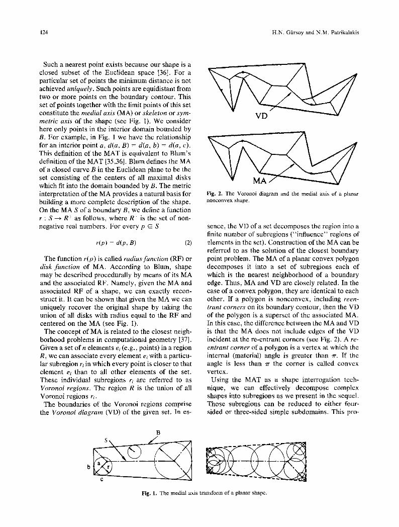
Such a nearest point exists because our shape is a closed subset of the Euclidean space [36]. For a particular set of points the minimum distance is not achieved uniquely. Such points are equidistant from two or more points on the boundary contour. This set of points together with the limit points of this set constitute the medial axis (MA) or skeleton or symmetric axis of the shape (see Fig. 1). We consider here only points in the interior domain bounded by B. For example, in Fig. 1 we have the relationship for an interior point a, d(a, B) = d(a, b) = d(a, c). This definition of the MAT is equivalent to Blum's definition of the MAT [35,36]. Blum defines the MA of a closed curve B in the Euclidean plane to be the set consisting of the centers of all maximal disks which fit into the domain bounded by B. The metric interpretation of the MA provides a natural basis for building a more complete description of the shape. On the MA S of a boundary B, we define a function r : S ~ R + as follows, where R + is the set of non- negative real numbers. For every p E S

r(p) = d(p, B) (2)

The function r(p) is called radius function (RF) or disk funct ion of MA. According to Blum, shape may be described procedurally by means of its MA and the associated RF. Namely, given the MA and associated RF of a shape, we can exactly recon- struct it. It can be shown that given the MA we can uniquely recover the original shape by taking the union of all disks with radius equal to the RF and centered on the MA (see Fig. 1).

The concept of MA is related to the closest neighborhood problems in computational geometry [37]. Given a set o fn elements ee (e.g., points) in a region R, we can associate every element ei with a particular subregion re in which every point is closer to that element ee than to all other elements of the set. These individual subregions re are referred to as Voronoi regions. The region R is the union of all Voronoi regions r;.

The boundaries of the Voronoi regions comprise the Voronoi diagram (VD) of the given set. In es-

Fig. 2. The Voronoi diagram and the medial axis of a planar nonconvex shape.

sence, the VD of a set decomposes the region into a finite number of subregions ("influence" regions of elements in the set). Construction of the MA can be referred to as the solution of the closest boundary point problem. The MA of a planar convex polygon decomposes it into a set of subregions each of which is the nearest neighborhood of a boundary edge. Thus, MA and VD are closely related. In the case of a convex polygon, they are identical to each other. If a polygon is nonconvex, including reentrant corners on its boundary contour, then the VD of the polygon is a superset of the associated MA. In this case, the difference between the MA and VD is that the MA does not include edges of the VD incident at the re-entrant corners (see Fig. 2). A reentrant corner of a polygon is a vertex at which the internal (material) angle is greater than rr. If the angle is less than 7r the corner is called convex vertex.

Using the MAT as a shape interrogation technique, we can effectively decompose complex shapes into subregions as we present in the sequel. Those subregions can be reduced to either four- sided or three-sided simple subdomains. This pro-

B

Fig. 1. The medial axis transform of a planar shape.


cess constitutes the starting phase of our FE meshing scheme, in which a complex shape is decomposed into coarse subdivisions.

3.2 A Computational Methodology for the Medial Axis Transform

In this section, we briefly present our methodology to compute the MAT of connected planar shapes bounded by closed curved boundaries. The boundary of a region (or shape) is defined by an exterior loop and one or more interior loops (i.e., contours), if the region of interest is multiply connected. Each loop of the boundary is composed of an ordered set of boundary elements (curve segments and vertices). The algorithm developed for the MAT computation covers straight line, circular arc, and general nonuniform rational B-spline (NURBS) boundary curves. Our method can also be easily extended to compute the MAT of the complement of a planar shape bounded by an arbitrary number of loops [2].

A loop is a union of a finite number of boundary elements which are ordered in such a manner that when the loop is traversed in the positive direction the interior of the shape lies to the right. An element of the boundary is either a reentrant vertex, which is associated with material angle greater than ~r, or a straight line segment, or a circular arc segment with arbitrary radius. Line and circular arc segments are bounded by two end vertices. There are also two distinct types of circular arc segments. When we traverse a boundary loop in the positive direction, if a circular arc segment is traversed in the clockwise direction with respect to its associated circle it is convex. On the other hand, if a circular arc is traversed in the counterclockwise direction it is concave.

In our approach, a free-form boundary curve (e.g., a Bezier or B-spline curve) is approximated within a prescribed tolerance using these three boundary element types [2]. In our algorithm, we use the curve approximation technique presented in [38]. Approx- imation of a curved boundary in terms of a set of straight line segments can give rise to artificial branches in MAT computation. Such artificial ef- fects can be counteracted by using a threshold technique [39]. For this purpose, we use a threshold angle which specifies the maximum value of the angle giving rise to an actual MA branch between two adjacent segments [2].

If the boundary contour of a planar shape is composed of reentrant vertices, straight line segments, and circular arcs, with arbitrary radii, then the MA of this shape, in general, consists of straight line

segments and arcs of conics (i.e., parabola, ellipse, and hyperbola [35]). The MA branch S(ei, ej) of two boundary elements e; and ej is the locus of the points equidistant from ei and e i. Descriptions of conic MA branches and their parametric representations, useful for tracing purposes, are presented in [2] and [32]. The conic branches of MA can degenerate to straight line segments or circles.

In our computational methodology, we can analyt- ically define the MA in terms of conic sections between two boundary elements. Determining end points on the MA, we obtain the MA branch associated with the two boundary elements. For this purpose, we make use of the fundamental offset process directed towards the interior of a region. This process is analogous to propagation of a grass-fire wave front towards the interior of a shape. The offset of distance h of the boundary B of a planar region R is the envelope of the union of all closed circular disks of radius h, the centers of which are points of B. This definition accounts for two curves on both sides of the boundary, inside and outside. We are interested only in the offset of the boundary in the interior of the shape.

Using the sign convention adopted, we observe that on an inward offset of the boundary loop, convex arcs shrink but concave arcs expand compared to the initial boundary shape. We also notice that a reentrant vertex can be regarded as a degenerate case of a concave circular arc with zero radius, because such a vertex gives rise to a finite arc segment on the offset contour.

Given the boundary contour of a region, our objective for the computation of the MAT is to determine inward offset distances and the associated branch points at which the topology of the contour changes. These are so called effective offset distances and effective branch points. Effective branch points are the end points of MA branches.

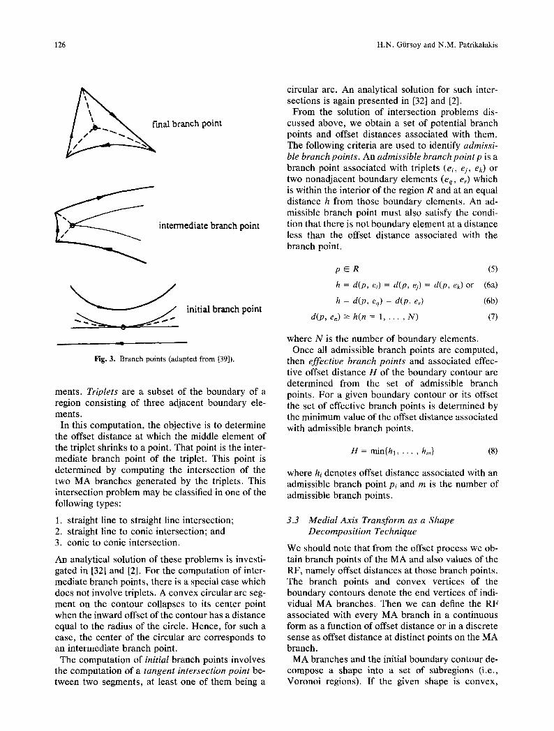
During the course of the offset process, there are three distinct types of branch points [39], (see Fig. 3). An initial branch point of a contour is a vertex at which precisely two nonadjacent elements of the offset contour are tangent to each other. An intermediate branch point of a contour is a vertex to which one or more elements of the nonvanishing offset shrink. Af inal branch point of a contour is a vertex which represents a vanishing offset contour. A final branch point is, in fact, a special case of an intermediate branch point and indicates the end of the offset process.

For the computation of intermediate and final branch points, the boundary contour is systemati- cally analyzed by using triplets of boundary ele-

126 H.N. Giarsoy and N.M. Patrikalakis

mal branch point

intermediate branch point

initial branch point

Fig. 3. Branch points (adapted from [39]).

ments. Triplets are a subset of the boundary of a region consisting of three adjacent boundary elements.

In this computation, the objective is to determine the offset distance at which the middle element of the triplet shrinks to a point. That point is the intermediate branch point of the triplet. This point is determined by computing the intersection of the two MA branches generated by the triplets. This intersection problem may be classified in one of the following types:

1. straight line to straight line intersection; 2. straight line to conic intersection; and 3. conic to conic intersection.

An analytical solution of these problems is investi- gated in [32] and [2]. For the computation of intermediate branch points, there is a special case which does not involve triplets. A convex circular arc segment on the contour collapses to its center point when the inward offset of the contour has a distance equal to the radius of the circle. Hence, for such a case, the center of the circular arc corresponds to an intermediate branch point.

The computation of initial branch points involves the computation of a tangent intersection point between two segments, at least one of them being a

circular arc. An analytical solution for such inter- sections is again presented in [32] and [2].

From the solution of intersection problems dis- cussed above, we obtain a set of potential branch points and offset distances associated with them. The following criteria are used to identify admissible branch points. An admissible branch point p is a branch point associated with triplets (ei, e i, e~) or two nonadjacent boundary elements (eq, er) which is within the interior of the region R and at an equal distance h from those boundary elements. An admissible branch point must also satisfy the condi- tion that there is not boundary element at a distance less than the offset distance associated with the branch point.

p E R (5)

h = d(p, el) = d(p, ej) = d(p, ek) or (6a)

h = d(p, eq) = d(p, er) (6b)

d(p, en) >- h(n = 1 . . . . . N) (7)

where N is the number of boundary elements. Once all admissible branch points are computed,

then effective branch points and associated effective offset distance H of the boundary contour are determined from the set of admissible branch points. For a given boundary contour or its offset the set of effective branch points is determined by the minimum value of the offset distance associated with admissible branch points.

H = rain{hi . . . . . hm} (8)

where hi denotes offset distance associated with an admissible branch point pi and m is the number of admissible branch points.

3.3 Medial Axis Transform as a Shape Decomposi t ion Technique

We should note that from the offset process we obtain branch points of the MA and also values of the RF, namely offset distances at those branch points. The branch points and convex vertices of the boundary contours denote the end vertices of individual MA branches. Then we can define the RF associated with every MA branch in a continuous form as a function of offset distance or in a discrete sense as offset distance at distinct points on the MA branch.

MA branches and the initial boundary contour decompose a shape into a set of subregions (i.e., Voronoi regions). If the given shape is convex,


Fig. 4. Decomposition of a nonconvex shape into simple subdomains.

those resulting subregions are also convex. For a nonconvex shape, some subregions are not convex. Introducing Voronoi edges and cuts at initial branch points as shown in Fig. 4, we can further subdivide such nonconvex subregions to obtain convex or pseudo-convex subregions. Voronoi edges of a given VD are the edges that are incident at re-entrant corners andflat vertices of the boundary contour of a planar shape. A fiat vertex of a boundary contour of a planar shape is a junction point of two adjacent boundary elements at which the interior angle is equal to ~r. A cut at an initial branch point is a straight line segment connecting two nonadjacent boundary elements across the initial branch point and orthogonal to these boundary elements. A pseudo-convex region is an area whose closed boundary can be offset until the area becomes nil without splitting the area into separate components. A pseudo-convex region involves no narrow bottle- neck type part, and the RF's associated with MA branches have no local minima other than the end points of the MA branches that generated the region.

As shown in Fig. 4, subregions can be further di- vided into topologically simple subdomains using a set of straight line segments which are indicated by the dotted lines in this figure. These lines are generated by projecting the branch points onto the boundary elements associated with the branch points. The resulting subdomains are either three- sided or four-sided subdomains.

3.4 An Algorithm for the Medial Axis Transform

Our computational methodology summarized in this section has led to an algorithm for MAT computation, whose pseudo-code is given below (see Algo- rithm 1). In our algorithm, boundary elements are treated independently to compute branch points. Then the effective offset distance and branch points

are determined using the set of branch points determined in this computation. We note that a contour may be associated with more than one effective branch point, though their effective offset distance must be the same. In the MAT computation, a contour may create more than one contour during the offset process, depending on the geometry of the contour. The MAT computation results in a set of Voronoi regions decomposing the shape. The Voro- noi regions are represented as faces in a boundary representation (B-Rep) model. The MA branches, Voronoi edges, and boundary elements are the bounding edges of the Voronoi regions. Discussion of data structures and representation techniques used in our algorithm and other implementation aspects of this scheme can be found in [2], [34], and [3].

4 An Automatic Mesh Generation Algorithm Based on the Medial Axis Transform

In this section, we present an automatic mesh generation scheme for multiply connected planar shapes based on the MAT, see also [2] for a more detailed description. Our algorithm is similar to the one proposed in [40] for polygonal domains. Our mesh generation scheme can, however, directly handle shapes with curved boundaries. This meshing process requires little user input or manual intervention, since it uses the MAT to automatically interrogate the geometric representation. There- fore, such a meshing scheme may prove to be a useful tool in design and analysis of complex engineering structures.

We first introduce fundamental aspects of a general two-step area meshing process. After that we present our methodology and meshing algorithm which incorporates the MAT with the FE mesh generation process.

4.I A General Two-Step Finite Element Triangulation Scheme

We present basic aspects of a two-step mesh generation process to obtain a two-dimensional triangular mesh. Theoretically, this process could be extended in an analogous way to three-dimensional cases using tetrahedra to discretize volumes. This approach is hybrid in the sense that it involves two distinct processes during finite element mesh generation. The first process decomposes the two-dimensional domain to be meshed into a set of topologically simple subdomains.

128 H.N. Gi~rsoy and N.M. Patrikalakis

Algorithm 1: Medial Axis Transform

input: Data of boundary contours (loops) of a region and threshold angle (TA).

output: List of medial axis (MA) branches, radius function, and list of Voronoi regions.

begin

Put initial contour(s) into contour queue;

while there is contour existing in contour queue { Get a contour from contour queue as current contour; /f interior of current contour is not nil {

for each segment, other than artificial ones { Compute admissible intermediate branch point (BP); if segment is a concave circular arc

Compute admissible initial BP(s); Put BP(s) into admissible BP list;

} Determine effective BP(s) using admissible BP list; Determine offset distance using an effective BP; for every convex vertex on current contour {

/f material angle of convex vertex -< TA { Compute segment of MA branch (S); Put S into MA branch list;

} } if effective BP is final

Stop computation for current contour; else {

Compute new offset contour(s); Put new contour(s) into contour queue;

} } else {

Compute MA branches of nil contour; Put MA branches into MA branch list;

}

Construct list for Voronoi regions;

end

for every boundary element of initial contour(s) { Create Voronoi region using MA branches; Put Voronoi region into list;

)

A simple subdomain in a simply connected convex or pseudo-convex region with one boundary loop which is composed of a sequence of either three or four edges. The second process triangulates individual simple subdomains generated by the first pro-

cess. Thus a triangular mesh of the domain is obtained by taking the union of all triangulated subdomains.

The mesh generator as input requires the geometry of a region R to be discretized as its input. This


input is usually in a B-Rep form which can be directly obtained from a B-Rep model or derived from a constructive solid geometry (CSG) representation by means of boundary evaluation.

Then initialization of discretization begins. A complex shape with reentrant corners and multiple internal holes is decomposed into simpler subdomains so that an admissible mesh with triangular elements of good shape characteristics can be generated. As a heuristic rule we require all triangular elements to approximately be equilateral triangles. The result of the decomposition process is a set of n convex or pseudo-convex subdomains ri whose union is the original shape R.

The subdomains generated in the previous decom- positions process are organized into an appropriate data structure for meshing. This representation con- tains adjacency information among all subdomains so that the triangular elements generated in adjacent subdomains satisfy compatibility requirements. In an admissible FE mesh composed of compatible elements, two adjacent elements share all nodes on the interface edge.

After the region is decomposed into a set of subdomains, each subdomain can be triangulated individ- ually

Ti = tz(ri) (9)

where the function /z(r;) embeds a triangular FE mesh Ti in subregion ri. These subdomains can be regarded as super finite elements from the FE discretization point of view. An approach for the triangulation of a simple subdomain can be based on discretization of the boundary of the subdomain followed by triangulation of the interior. The discretization of the boundary requires specification of mesh size and density. The discretization of the subdomain boundaries also assures compatibility between adjacent elements in different subdomains. The FE mesh T of the region R is the union of all FE meshes Ti embedded in all subdomains r~.

T = U~_l Ti (10)

It is worth noting that other mesh generation schemes (such as mapping, recursive decomposition, and point insertion followed by triangulation techniques) can also be used to discretize these individual simple subdomains.

Automatic triangulation of a complex shape may generate finite elements with unfavorable shape properties. Regions with highly nonuniform shape characteristics, closely spaced holes, wavy bound-

aries, etc can give rise to very irregular meshes. It is common practice to apply smoothing to the mesh generated by triangulation in order to improve irregular shapes. Various schemes are available for the mesh smoothing process such as Laplacian and isoparametric methods [9]. Our smoothing technique to satisfy this objective is an iterative process in which the position of an interior node is incrementally changed by averaging its coordinates and the coordinates of all adjacent nodes.

Depending on the problem at hand, a FE discretization may need local refinement in order to improve numerical results. Before the first FEA, a coarse mesh should be locally refined in regions close to boundary segments associated with boundary conditions such as fixed nodes, concentrated loads, and also singularities arising from fixed and reentrant corners. Also in an adaptive FEA using a posteriori error indicators [41], finite elements which give rise to large error should be refined in order to obtain better numerical results in subsequent analysis steps. For local refinement based on the h-convergence approach, triangular elements can be bisected across their longest edge. This method allows generation of compatible meshes, and at the same time does not degrade the shape characteristics of triangular elements. The following pseudo-code summarizes the main steps involved in this two-step finite element mesh generation process (see Algorithm 2).

4.2 The Finite Element Mesh Generation Scheme Based on the Medial Axis Transform

Using the two-step meshing methodology introduced in the previous section, we have developed a meshing scheme based on the MAT, which automatically discretizes a two-dimensional shape into a set of triangular elements. This meshing scheme ac- cepts the MAT of a shape as its input and generates complete FE mesh information. Major steps of this scheme are presented in the following sections.

4.2.1 Decomposition o f a region by means o f the medial axis transform

Due to the nature of the MAT, every boundary element is associated with a unique Voronoi region of the shape. We can subdivide a Voronoi region into simple subdomains in such a way that a portion of the boundary element is associated with only one MA branch on the boundary of the Voronoi region. Thus, we obtain a coarse discretization of the shape. Such a coarse discretization can be effectively used as a FE mesh in a p-version FEA. An-

130 H.N. Giarsoy and N.M. Patrikalakis

input: output: begin

end

Algorithm 2: A General Two-Step Finite Element Meshing Scheme

Boundary representation model of a domain to be meshed. Finite element mesh composed of triangles.

Decompose domain into topologically simple subdomains; Generate nodes along boundaries of subdomains; for each subdomain

Create a triangular finite element mesh; for each subdomain

/f refinement is required Refine mesh of subdomain without violating compatibility;

if shape characteristics of mesh are not good enough Smooth mesh;

other possible application of this approach is that we can easily identify subdomains associated with significant boundary conditions. Thus we determine areas for local mesh refinement in a direct and efficient manner. As a result, this meshing scheme directly yields discretizations with a spatial addressability property. Such a feature is very useful for adaptive FEA methods.

Given a Voronoi region, the region can be further subdivided so that each MA branch on the perime- ter of the Voronoi region can be mapped onto a unique finite portion of the boundary element associated with the Voronoi region. The mapping is done by means of a projection process. In a degenerate case, if the boundary element is a reentrant corner, all MA branches of the Voronoi region associated with this vertex are mapped onto this vertex.

The segmentation of the boundary is carried out by computing the projections of the end points of MA branches (i.e. branch points) onto the boundary element associated with those branches, (see Fig. 5). This decomposition process results in a set of subdomains with simple topology. These subdomains are either three- or four-sided subdomains, (see Fig. 5). Three-sided subdomains arise at terminal branches of the MA and, possibly, at reentrant (nonconvex) vertices (see Figs. 4 and 5). If a potential three-sided subdomain is very narrow, (i.e., with a small acute angle), this subdomain is not generated and the adjacent four-sided subdomain is merged with this three-sided subdomain. Four- sided subdomains arise for all other branches of the MA. Such a decomposition process also allows us to effectively use local lengths scales of a shape. In this work, we use the largest value of the radius function for a given subdomain as the local length scale associated with that subdomain. This information, in turn, is used to determine the length dimen-

sion of triangular finite elements discretizing the subdomain. We also make use of the value of radius function at initial branch points to determine the local length scale of constriction.

4.2.2 Processing of the subdomains obtained fi'om the medial axis transform

The MAT based process of the previous section decomposes a complex shape into a set of topologically simple three- or four-sided subdomains. Al- though these subdomains are topologically simple, the lengths of their edges may, sometimes, turn out to vary significantly. For example, very narrow subdomains involving angles which are very differ-

Fig. 5. Shape decomposition by means of the medial axis transform.


ent from rr/3 may be occasionally generated. Pres- ence of such badly shaped subdomains makes it dif- ficult to create a FE discretization composed of triangles with good shape characteristics. As a rule, we require that all triangular elements closely re- semble equilateral triangles. Although we do not use quadrilateral elements in our meshing scheme, the optimum quadrilateral element shape is the square. The objective of these heuristic rules is that a well shaped finite element does not have a bias towards a particular direction in a FE mesh layout. Such a requirement can be expressed in terms the aspect ratios of elements. A measure of aspect ratio may be defined using the MA and radius function of a triangular element. The aspect ratio (AR) defined as the ratio o f length o f longest MA branch to the maximum value o f the radius function also effectively accounts for skewness of elements.

We illustrate these abnormalities involved in shape decomposition based on the MAT using a simple shape. Figure 6 shows a rectangle whose longer dimension D is a variable and the shorter dimension is constant, d = 2a. In Fig. 7, corresponding to D = 2a, (i.e. a square), the solid line is the MA of the rectangle and dotted lines represent discretization of the region in terms of triangular elements. Here we observe that the triangular elements exhibit good shape characteristics. The aspect ratio of the triangles is V~. If we start to increase D, the MAT decomposition will give rise to two very narrow subdomains. If2a < D < 5a/2, the discretization of those subdomains produces triangles with poor shape characteristics (i.e., AR > 2.24, see Fig. 8). In Fig. 8, triangulation of the rec- tangular domain is carried out using our mesh generation method presented in the subsequent sec-

d = 2 a

F- x~ . / 1 '

x ~ / D

_A

D = d

Fig. 7. Finite element mesh of the parametric shape.

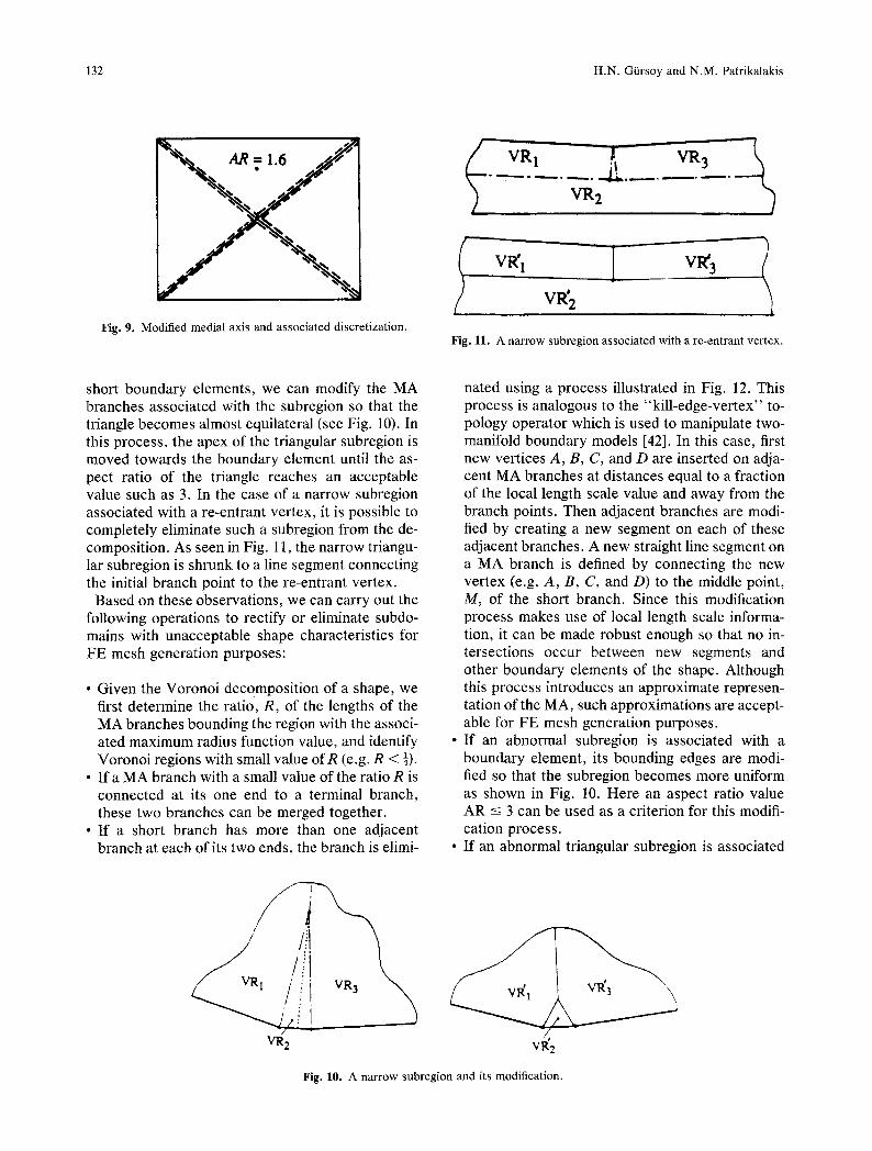
tions. For the time being, let us consider only shape characteristics of these triangular elements. We can identify a situation which gives rise to badly shaped elements using the ratio, R, of the length of associated MA branch to the maximum value of radius function, in this particular case 0 -< R < �89 To rectify this abnormality, the short MA branch needs to be processed. For example, as seen in Fig. 9, we can construct an approximate MA by eliminating the short MA branch, and obtain a modified decomposition. In this example, the triangle is of aspect ratio AR = 1.6 which is better than the previous value.

Short boundary elements and re-entrant vertices with angles only slightly above 7r also give rise to very narrow triangular Voronoi regions, (see Figs. 10 and 11). Such cases arise frequently for high accuracy approximations of a curved shape with linear segments. For the narrow subregion due to

d - 2 a

I

L L !

d - 2a

n

s j I f

d I

D - 5 a

j = 2 . 2 4

Fig. 6. A simple parametric shape. Fig. 8. Finite elements with high aspect ratios,

132 H.N. Giirsoy and N.M. Patrikalakis

. f I . . . . .

Fig. 9. Modified medial axis and associated discretization. Fig. 11. A narrow subregion associated with a re-entrant vertex.

short boundary elements, we can modify the MA branches associated with the subregion so that the triangle becomes almost equilateral (see Fig. 10). In this process, the apex of the triangular subregion is moved towards the boundary element until the aspect ratio of the triangle reaches an acceptable value such as 3. In the case of a narrow subregion associated with a re-entrant vertex, it is possible to completely eliminate such a subregion from the decomposition. As seen in Fig. 11, the narrow triangular subregion is shrunk to a line segment connecting the initial branch point to the re-entrant vertex.

Based on these observations, we can carry out the following operations to rectify or eliminate subdomains with unacceptable shape characteristics for FE mesh generation purposes:

�9 Given the Voronoi decomposition of a shape, we first determine the ratio, R, of the lengths of the MA branches bounding the region with the associated maximum radius function value, and identify Voronoi regions with small value of R (e.g. R < k).

�9 If a MA branch with a small value of the ratio R is connected at its one end to a terminal branch, these two branches can be merged together.

�9 If a short branch has more than one adjacent branch at each of its two ends, the branch is elimi-

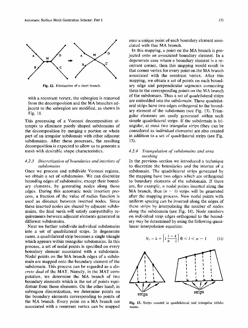
nated using a process illustrated in Fig. 12. This process is analogous to the "kill-edge-vertex" topology operator which is used to manipulate two- manifold boundary models [42]. In this case, first new vertices A, B, C, and D are inserted on adjacent MA branches at distances equal to a fraction of the local length scale value and away from the branch points. Then adjacent branches are modified by creating a new segment on each of these adjacent branches. A new straight line segment on a MA branch is defined by connecting the new vertex (e.g. A, B, C, and D) to the middle point, M, of the short branch. Since this modification process makes use of local length scale information, it can be made robust enough so that no in- tersections occur between new segments and other boundary elements of the shape. Although this process introduces an approximate representation of the MA, such approximations are acceptable for FE mesh generation purposes. If an abnormal subregion is associated with a boundary element, its bounding edges are modified so that the subregion becomes more uniform as shown in Fig. 10. Here an aspect ratio value AR -< 3 can be used as a criterion for this modification process. If an abnormal triangular subregion is associated

//i

J

VR 2 VR2

Fig. 10. A narrow subregion and its modification.


Fig. 12. Elimination of a short branch.

with a reentrant vertex, the subregion is removed from the decomposition and the MA branches adjacent to the subregion are modified, as shown in Fig. 11.

This processing of a Voronoi decomposition at- tempts to eliminate poorly shaped subdomains of the decomposition by merging a portion or whole part of an irregular subdomain with other adjacent subdomains. After these processes, the resulting decomposition is expected to allow us to generate a mesh with desirable shape characteristics.

4.2.3 Discretization of boundaries and interiors of subdomains

Once we process and subdivide Voronoi regions, we obtain a set of subdomains. We can discretize bounding edges of subdomains, except their boundary elements, by generating nodes along those edges. During this automatic node insertion process, a fraction of the value of radius function is used as distance between inserted nodes. Since these inserted nodes are shared by adjacent subdomains, the final mesh will satisfy compatibility requirements between adjacent elements generated in different subdomains.

Next we further subdivide individual subdomains into a set of quadrilateral strips. In degenerate cases, a quadrilateral strip becomes a single triangle which appears within triangular subdomains. In this process, a set of nodal points is specified on every boundary element associated with a subdomain. Nodal points on the MA branch edges of a subdomain are mapped onto the boundary element of the subdomain. This process can be regarded as a discrete dual of the MAT. Namely, in the MAT computation, we determine the MA branch of two boundary elements which is the set of points equidistant from those elements. On the other hand, in subregion discretization, we determine points on the boundary elements corresponding to points of the MA branch. Every point on a MA branch not associated with a reentrant vertex can be mapped

onto a unique point of each boundary element associated with that MA branch.

In this mapping, a point on the MA branch is pro- jected onto an associated boundary element. In a degenerate case where a boundary element is a reentrant corner, then this mapping would result in that corner vertex for every point on the MA branch associated with the reentrant vertex. After this mapping, we obtain a set of points on each boundary edge and perpendicular segments connecting them to the corresponding points on the MA branch of the subdomain. Thus a set of quadrilateral strips are embedded into the subdomain. These quadrilateral strips have two edges orthogonal to the boundary element of the subdomain (see Fig. 13). Trian- gular elements are easily generated within such simple quadrilateral strips. If the subdomain is triangular, at most two triangular strips (they can be considered as individual elements) are also created in addition to a set of quadrilateral strips (see Fig. 13).

4.2.4 Triangulation of subdomains and area meshing

In the previous section we introduced a technique to discretize the boundaries and the interior of a subdomain. The quadrilateral strips generated by the mapping have two edges which are orthogonal to boundary elements of the subdomain. If there are, for example, n nodal points inserted along the MA branch, then (n - 1) strips will be generated after the mapping process. New nodal points with uniform spacing can be inserted along the edges of these strips by interpolating the number of nodes along the subdomain (see Fig. 14). Node numbers on individual strip edges orthogonal to the boundary may be determined by using the following quasi- linear interpolation equation:

[i l - k ] N ~ = k + | n_ l l O < i < n - I (11)

strips strips

Fig. 13. Strips created in quadrilateral and triangular subdomains.

134 H.N. G~rsoy and N.M. Patrikalakis

n

l I I i rUT,',',!

I1

I - , , . i .t

I l

', : • 1 I I

1 I

I m l i p

/ NJ-k 1 Fig. 14. Node generation procedure within a subdomain.

where N; is the number of nodes on the ith edge connecting a point on the boundary element to a corresponding point on the branch at integer position i in the point sequence; k and l are the numbers of nodes on the extreme oblique edges of the subdomain; n is the number of nodes on the MA branch; and [ ] denotes ceiling. In Fig. 14, the left and right "vertical" edges are oblique to the bottom edge because of merging two triangular subdomains with high aspect ratio with this quadrilateral subdomain.

After inserting all nodes along the edges of the strips of a subdomain, triangulation of a subdomain can be carried out by triangulating individual strips. If the subdomain is triangular it can be transformed to a quadrilateral by removing a triangular element (which is the degenerate strip of this subdomain) from the subdomain. Triangulation of the quadrilateral strips is a relatively straightforward process which involves matching of appropriate nodes on two opposite edges of the strip. Several techniques have also been proposed for triangulation of such strips [10]. The edges of the strips are perpendicular to boundary elements of the subdomain. For a given strip, the four corner vertices are interrogated to determine the one associated with the largest interior angle. Once this vertex is identified, it is connected to an appropriate vertex on the other edge of the strip such that a triangular element is extracted from the strip at the end of this process (see Fig. 17). Then, this process is applied to the remaining part of the strip. Thus a set of triangles are generated by removing triangles from the strip one at a time. In our current implementation, the difference of node numbers on opposite edges of a strip is as large as 3 but could easily be modified to other values.

The triangulation process we use in discretization of individual subdomains is an efficient and robust technique. Our meshing algorithm, however, is not limited only to this scheme. We could effectively use other triangulation methods (e.g. Delaunay triangulation [16]). In such an approach, we could define a individual subdomain using MA branches and boundary element associated with the subdomain. In that triangulation process, nodes on the boundary and in the interior of the subdomain would be "injected" into the mesh one at a time. In this case, the meshing scheme based on our shape decomposition approach would also result in better computational efficiency, since we break down the overall triangulation task into a set of smaller tasks. In the meshing process, the triangulation of a set of subdomains with a small fraction of the total number of nodes could be carried out more efficiently than the triangulation of the whole domain using all nodes.

After all subdomains of a shape are triangulated, mesh smoothing and local refinement processes can be applied to the resulting mesh in order to improve its shape characteristics. The following pseudo- code summarizes the main steps involved in our finite element mesh generation process based on MAT (see Algorithm 3). Data structures used and techniques developed for these processes are re- ported in [3].

Figures 15 through 18 illustrate the steps involved in our FE mesh generation scheme. Figure 15 illus- trates the MA of the multiply connected planar shape. Subdivision of the region and nodes inserted along the edges of the subdomains are illustrated in Fig. 16. Figure 17 shows the triangulation process within a subdomain. Finally, the resulting mesh is shown in Fig. 18.

Fig. 15. A planar multiply connected shape and its medial axis.

Fig. 16. Region subdivision and boundary discretization.


input: output: begin

end

Algorithm 3: A Two-Step FE Meshing Based on Medial Axis Transform

Data of boundary contour(s) of a region. List of triangular finite elements.

Construct medial axis, list of Voronoi regions using Algorithm 1; Create list for simple subdomains; for each three sided Voronoi region

Add region into subdomain list; for each remaining Voronoi region {

Subdivide region into three four-sided subdomains; Add subdomains into subdomain list;

} for each edge between adjacent subdomains

Generate uniformly distributed nodes; Create list for triangular elements; for each subdomain in list {

/f subdomain is four sided { Generate set of quadrilateral strips; Triangulate strips in quadrilateral subdomain;

} tf subdomain is three sided {

Generate set of strips; Convert triangular subdomain into quadrilateral by extracting one

degenerate triangular strip as a triangular element; Triangulate strips in remaining quadrilateral subdomain;

} Add triangles into list;

} /f shape of triangular elements requires improvement

Smooth mesh;

4.3 Complexity Estimates of the Medial Axis Transform and Meshing Processes

A basic complexi ty analysis of our MAT algorithm follows. We need to consider all O(n 2) pairs of boundary elements to determine points of closest

f stops

Sh - . v

Fig. 17. Triangulation of an individual subdomain.

approach. Then all such points which pass local tests of being possible initial branch points, must be checked against all other boundary elements O(n) to determine if they are admissible (i.e. not closer to any other elements). At worst, therefore, the time complexity is O(n3). This estimate assumes that local tests for possible initial branch points do not reduce the order of magnitude of the number of such points. Experiments indicate that this is an overly pessimistic assumption.

The coarse triangular mesh generation process is

\\// 4///!/

\ / / / < / /

Fig. 18. Finite element mesh of a planar multiply connected region.

136 H.N. Giirsoy and N.M. Patrikalakis

an O(m) process with respect to the total number of triangular elements, m, being generated. Triangula- tion of individual subdomains has a linear time complexity with respect to the number of elements generated. The reason is that our meshing scheme is geometrically based and no search operations are carried out during the meshing process as, for example, in topologically based schemes. Thus this approach gives rise to a linear running time complexity.

Considering the overall performance of our implementation, the overhead involved in our MAT algorithm is subdominant with respect to the mesh creation and refinement time complexity. In a typical mesh generation problem n ~ m and therefore the bulk of the computational effort is spent for actual mesh generation and refinement processes, which exhibit a linear time complexity. Timing results of several test cases obtained using our computer implementation confirm these observations [2,3].

5 Summary and Conclusions

We have presented the MAT as a shape interrogation method and an algorithm to compute the MA of two-dimensional shapes with curved boundaries. The two-dimensional shape can either be planar objects or the parameter space of a curved trimmed surface patch. For the latter case, mapping of the MA to three-dimensional space via the surface equation allows surface discretization. This scheme can effectively extract several important shape characteristics in an automated manner. We have also presented a new FE mesh generation scheme based on MAT. Several important advantages of this scheme include the capability to extract shape characteristics and length scales in a fully automated manner, a direct way of defining super finite elements and a substructuring capability, and spatial addressability of resulting discretizations created by the scheme.

Extension of these techniques to higher dimensions (MAT on curved surfaces and within three- dimensional volumes) is feasible [2,43]. However, such extension is expected to be computationally intensive due to substantial increases in combinato- rial and algebraic complexity of the process in higher dimensions.

MAT computations on general curved surfaces using an appropriate distance metric would require geodesics. MAT of general three-dimensional closed volumes is an active research problem. In addition to the computational complexity of the

MAT in this case, the MA of an object in three dimensions, in general, involves mixed dimensional entities (such a MA generally comprises connected distinct vertices, curved edge segments, and surface patches as MA branches). Thus, representation of such a complex structure within a volume would require sophisticated B-Rep techniques ca- pable of handling non-two-manifold situations [44- 46].

Even though there are major difficulties in MAT computation in higher dimensions, MAT is a very rich topic involving interesting research problems. This technique promises elegant solutions to many potential applications in engineering design and analysis [2,34].

Acknowledgments

Funding for this research was obtained in part from MIT Sea Grant College Program (grant number NA90AA-D-SG-424) and the Office of Naval Research in the United States (grant numbers N00014-87-K-0462 and N000-91-J-1014). Professor C. M. Hoff- mann provided valued assistance on the complexity analysis of our MAT algorithm.

References

1. Blum, H., (1967) A transformation for extracting new de- scriptors of shape, models for the Perception of Speech and Visual Form, Weinant Wathen-Dunn (Editor), MIT Press, Cambridge, MA, 362-381

2. Gursoy, H.N., (1989) Shape interrogation by medial axis transform for automated analysis, PhD Dissertation, Massa- chusetts Institute of Technology, Cambridge, MA

3. Gursoy, H.N., Patrikalakis, N.M., (1992) A coarse and fine element mesh generation scheme based on medial axis transform: Part II implementation, Engineering with Computers, Springer-Verlag, New York

4. Ho-Le K., (1988) Finite element mesh generation methods: A review and classification, Computer-Aided Design, 20, 1, 27-38

5. Shephard, M.S., (1988) Approaches to the automatic generation and control of finite element meshes, ASME Applied Mechanics Review, 41, 4, 169-184

6. Zienkiewicz, O.C., Phillips, D.V., (1971) An automatic mesh generation scheme for plane and curved surfaces by isoparametric coordinates, International Journal for Numerical Methods in Engineering, 7, 461-477

7. Gordon, W.J., (1973) Construction of curvilinear coordinate systems and applications to mesh generation, International Journal for Numerical Methods in Engineering, 7, 461-477

8. Cook, W.A., (1974) Body oriented (natural) coordinates for generating three dimensional meshes, International Journal for Numerical Methods in Engineering, 8, 27-43

9. Herrmann, L.R., (1976) Laplacian-isoparametric grid generation scheme, Journal of Engineering Mechanics Division Proceedings of the ASCE, 102, EM5, 749-756

10. Imafuku, I., Kodera, Y., Sayawaki, M., (1980) A general- ized automatic mesh generation scheme for finite element


method, International Journal for Numerical Methods in En- gineering, 15,713-731

11. Cavendish, J.C., Hall, C.A., (1984) A new class of transi- tional blended finite elements for analysis of solid structures, International Journal for Numerical Methods in Engineering, 20, 241-253

12. Wellford, L.C., Gorman, M.R., (1988) A finite element tran- sitional mesh generation procedure using sweeping func- tions, International Journal for Numerical Methods in Engi- neering, 26, 2623-2643

13. Frederick, C.O., Wang, Y.C., Edge, F.W., (1970) Two-dimensional automatic mesh generation for structural analysis, International Journal for Numerical Methods in Engineering, 2, 1, 133-144

14. Van-Phal, N., (1982) Automatic mesh generation with tetra- hedron elements, International Journal for Numerical Meth- ods in Engineering, 18,273-280

15. Lee, Y.T., De Pennington, A., Shaw, N.K., (1984) Auto- matic finite-element mesh generation from geometric model--a point-based approach, ACM Transactions on Graphics, 4, 287-311

16. Cavendish, J.C., Field, D.A., Frey, W.H., (1985) An approach to automatic three-dimensional finite element mesh generation, International Journal for Numerical Methods in Engineering, 21,329-347

17. Lo, S.H., (1985) A new mesh generation scheme for arbitrary planar domains, International Journal for Numerical Methods in Engineering, 21, 8, 1403-1426

18. Joe, B., (1986) Delaunay triangular meshes in convex polygons, SIAM Journal on Scientific and Statistical Computing, 7, 2, 514-539

19. Field, D.A., (1986) Implementing Watson's algorithm in three dimensions, Proceedings of the Second Annual ACM Symposium on Computational Geometry, 246-259

20. Schroeder, W.J., Shephard, M.S., (1988)Geometry-based fully automatic mesh generation and the delaunay triangulation, International Journal for Numerical Methods in Engi- neering, 26, 2503-2515

21. Bykat, A., (1976) Automatic generation of triangular grid: I--Subdivision of a general polygon into convex subregions. II--Triangulation of convex polygons, International Journal for Numerical Methods in Engineering, 10, 1329-1324

22. Sadek, E., (1980) A scheme for the automatic generation of triangular finite elements, International Journal for Numeri- cal Methods in Engineering, 15, 1813-1822

23. Wordenweber, B., (1984) Finite element analysis for the na- ive user, Solid Modeling by Computers, From Theory to Applications, Plenum Press, NY., M.S. Pickett, J.W. Boyse (Editors), 81-101

24. Woo, T.C., Thomasma, T., (1984) An algorithm for generating solid elements in objects with holes, Computers & Struc- tures, 18, 2, 333-342

25. Joe, B., Simpson, R.B., (1986) Triangular meshes for regions of complicated shape, International Journal for Numerical Methods in Engineering, 23, 5,751-778

26. Chae, S.W., (1988) On the automatic generation of near- optimal meshes for three-dimensional linear elastic finite element analysis, PhD Dissertation, Massachusetts Institute of Technology, Cambridge, MA

27. Yerry, M.A., Shephard, M.S., (1984) Automatic three-dimensional mesh generation by the modified octree technique, International Journal for Numerical Methods in Engi- neering, 20, 1965-1990

28. Kela, A., Perucchio, R., Voelcker, H., (1986) Towards automatic finite element analysis, ASME Computers in Mechani- cal Engineering, 5, 1, 57-71

29. Baehmann, P.L., Wittchen, S.L., Shephard, M.S., Grice, K.R., Yerry M.A., (1987) Robust, geometrically based, automatic two-dimensional mesh generation, International Journal for Numerical Methods in Engineering, 24, 8, 1043- 1078

30. Sluiter, M.L.C., Hansen, D.C., (1982) A general purpose automatic mesh generator for shell and solid finite elements, Computers in Engineering, L.E. Hulbert (Editor), ASME, New York, 3, 29-34

31. Bykat, A., (1983) Design of a recursive, shape controlling mesh generator, International Journal for Numerical Meth- ods in Engineering, 19, 9, 1375-1390

32. Patrikalakis, N.M., Gursoy, H.N., (1988) Skeletons in shape feature recognition for automated analysis, MIT Ocean En- gineering Design Laboratory Memorandum 88-4

33. Patrikalakis, N.M., Gursoy, H.N., (1989) Shape feature recognition by medial axis transform, MIT Ocean Engineering Design Laboratory Memorandum 89-1

34. Patrikalakis, N.M., Gursoy, H.N., (1990) Shape interrogation by medial axis transform," Advances in Design Auto- mation 1990, Volume One: Computer Aided and Computa- tional Design, B. Ravani (Editor), ASME, NY, 77-88

35. Blum, H., (1973) Biological shape and visual science (Part I)," Journal of Theoretical Biology, 38, 205-287

36. Wolter, F.-E., (1985) Cut loci in bordered and unbordered riemannian manifolds, PhD Dissertation, Technical Univer- sity of Berlin, Department of Mathematics

37. Preparata, F.P., Shamos, M.I., (1985) Computational geometry: An introduction, Springer-Verlag, New York

38. Patrikalakis, N.M., (1989) Approximate conversion of rational splines," Computer Aided Geometric Design, 2, 6, 155-165

39. Montanari, U., (1969) Continuous skeletons from digitized images, Journal of the Association for Computing Machin- ery, 16, 4, 534-549

40. Srinivasan, V., Nackman, L.R., Tang, J-M, Meshkat, S.N., (1990) Automatic mesh generation using the symmetric axis transformation of polygonal domains, Research Report, IBM Research Division, RC 16132

41. Babuska, I., Zienkiewicz, O.C., Gago, J., Oliveira, E.R.A., (1986) Accuracy estimates and adaptive refinements in finite element computations, John Wiley, Chichester, England

42. Mantyla, M., (1988) An Introduction to Solid Modeling, Computer Science Press, Rockville, Maryland

43. Hoffmann, C.M., (1990) How to construct the skeleton of CSG objects, Technical Report, CSD-TR-1014, Purdue Uni- versity

44. Weiler, K.J., (1986) Topological structures for geometric modeling, PhD Dissertation, Rensselaer Polytechnic Insti- tute, Troy, NY

45. Gursoz, L., Choi, Y. and Prinz, F.B., (1990) Vertex-based representation of non-manifold boundaries, Geometric Mod- eling for Product Engineering, M.J. Wozny, J.U. Turner and K. Preiss (Editors), North-Holland, NY, 107-130

46. Rossignac, J.R., O'Connor, M.A., (1990) SGC: A dimension-independent model for pointsets with internal structures and incomplete boundaries, Geometric Modeling for Product Engineering, M.J. Wozny, J.U. Turner and K. Pre- iss (Editors), North-Holland, NY, 145-180

Engineering C61 puters - MITweb.mit.edu/deslab/pubs/gurs1.pdf · Engineering with Computers 8,...

Documents

Transcript of Engineering C61 puters - MITweb.mit.edu/deslab/pubs/gurs1.pdf · Engineering with Computers 8,...