
Computational Study of Solvent Effects on the Stability of ...
116
Master’s Degree programme in Science and Technology of Bio and Nanomaterials Computational Study of Solvent Effects on the Stability of Native Structures in Proteins Supervisor Ch. Prof. Achille Giacometti Assistant supervisor Dr. Tatjana Škrbić Graduand Emanuele Petretto Matriculation Number 855446 Academic Year 2016/2017
Transcript of Computational Study of Solvent Effects on the Stability of ...
Master’s Degree programme inScience and Technology of Bio and Nanomaterials
Computational Study of SolventEffects on the Stability of Native
Structures in Proteins
SupervisorCh. Prof. Achille Giacometti
Assistant supervisorDr. Tatjana Škrbić
GraduandEmanuele Petretto Matriculation Number 855446
Academic Year 2016/2017
Contents
Introduction iii
1 Proteins 11.1 Amino acids . . . . . . . . . . . . . . . . . . . . . . . . . . . . . . . . 21.2 Forces . . . . . . . . . . . . . . . . . . . . . . . . . . . . . . . . . . . 51.3 Primary structure of protein . . . . . . . . . . . . . . . . . . . . . . . 71.4 Secondary structure of protein . . . . . . . . . . . . . . . . . . . . . . 9
1.4.1 α-helix . . . . . . . . . . . . . . . . . . . . . . . . . . . . . . . 91.4.2 β-sheet . . . . . . . . . . . . . . . . . . . . . . . . . . . . . . . 11
1.5 Tertiary and quaternary structure . . . . . . . . . . . . . . . . . . . . 121.6 Protein folding . . . . . . . . . . . . . . . . . . . . . . . . . . . . . . 131.7 Protein solubility and stability . . . . . . . . . . . . . . . . . . . . . . 171.8 Protein stability in solvent other than water . . . . . . . . . . . . . . 23
2 Computational methods 272.1 Molecular dynamics . . . . . . . . . . . . . . . . . . . . . . . . . . . . 28
2.1.1 Force field . . . . . . . . . . . . . . . . . . . . . . . . . . . . . 282.1.2 Bonded interaction . . . . . . . . . . . . . . . . . . . . . . . . 292.1.3 Non-Bonded interaction . . . . . . . . . . . . . . . . . . . . . 312.1.4 Free energy . . . . . . . . . . . . . . . . . . . . . . . . . . . . 322.1.5 General simulation routine . . . . . . . . . . . . . . . . . . . . 342.1.6 Water models . . . . . . . . . . . . . . . . . . . . . . . . . . . 38
2.2 Monte Carlo simulations . . . . . . . . . . . . . . . . . . . . . . . . . 392.3 Metropolis Method . . . . . . . . . . . . . . . . . . . . . . . . . . . . 40
3 Solvation free energy of amino acids side chains 433.1 Free energy . . . . . . . . . . . . . . . . . . . . . . . . . . . . . . . . 443.2 Bennett’s acceptance ratio method . . . . . . . . . . . . . . . . . . . 463.3 Experimental data for the amino acids . . . . . . . . . . . . . . . . . 47
i

ii CONTENTS
3.4 Free energy calculation of single amino acid . . . . . . . . . . . . . . 483.4.1 Free energy calculation routine . . . . . . . . . . . . . . . . . 49
3.5 Results . . . . . . . . . . . . . . . . . . . . . . . . . . . . . . . . . . . 49
4 Protein folding in non water solvent 634.1 Model . . . . . . . . . . . . . . . . . . . . . . . . . . . . . . . . . . . 654.2 Entropic excluded-volume effect . . . . . . . . . . . . . . . . . . . . . 674.3 The energetic component . . . . . . . . . . . . . . . . . . . . . . . . . 714.4 Decoys preparation . . . . . . . . . . . . . . . . . . . . . . . . . . . . 724.5 Sampling . . . . . . . . . . . . . . . . . . . . . . . . . . . . . . . . . . 744.6 Compactification . . . . . . . . . . . . . . . . . . . . . . . . . . . . . 774.7 Checking compactification and reconstruction . . . . . . . . . . . . . 774.8 Stride analysis . . . . . . . . . . . . . . . . . . . . . . . . . . . . . . . 834.9 Results . . . . . . . . . . . . . . . . . . . . . . . . . . . . . . . . . . . 85
Conclusion and perspective 91
A Experimental methods 95A.1 X-ray crystallography . . . . . . . . . . . . . . . . . . . . . . . . . . . 95A.2 Calorimetry . . . . . . . . . . . . . . . . . . . . . . . . . . . . . . . . 97
A.2.1 Differential scanning calorimetry . . . . . . . . . . . . . . . . 97A.2.2 Isothermal titration calorimetry . . . . . . . . . . . . . . . . . 98
B General algorithm for decoys construction 101
Introduction
Water is one of the main components of the all ecosystems and the basis for life-as-we-know-it. Some important properties of water, beside that of the other all simpleorganic compounds, has been fundamental to the abiogenesis. These are, for exam-ple, the wide range temperature in which it can be found in liquid state, the heatcapacity, useful for thermoregulation, and the high solvent power that is useful tospread and diffuse solute. Polar character, due by the charge dislocation actuated bythe electronegative oxygen atom, the capability to generate hydrogen bonds and thecorresponding network, and the self-ionization that allows water to donate or acceptH+ ion, provides to water a large chemical activity. Metabolic pathway reaction areintimately connected to water as solvent, reactant or product. Evolution shapedbiomolecule activity and functionality, from the first self-replicating and catalyticRNA molecules to the neurotransmitter receptor associated with the membrane inpost synaptic cells, in water environment. Understanding how life could have beenwithout water is one of the most challenging issues in astrobiology. This problem isof considerable interest even on earth, as other solvents might be competitive withwater. A canonical example can be the methane (CH4) composed by the to mostcommon element in the universe: carbon and hydrogen. In this environment, so-luted biomolecule do not occur into hydrolysis reactions, allowing a larger chemicalstability, but subsequently, this solvent is not able behave as the solvent, reactant orproduct feature in the water. Second example is provided by protein living in mem-brane within hydrophobic environment. Focusing on the electrostatic interaction, acompletely apolar solvent as methane, could make the intrasolute or solute-soluteelectrostatic interaction more favorable than in water since this could disrupt theseinteraction. A possible way to understand this kind of dynamics is study the sta-bility and solubility of molecule in this new solvents. Use proteins to proceed onthis exploration could permit to have a multiple point of view to understand thephysico-chemical basis of protein. Protein folding and stability are intimate corre-lated since the native conformation of a protein, capable to provide a wide diversityof function, is even the most stable. Exploring proteins stability in other polar or
iii

iv INTRODUCTION
non-polar solvent such as ethanol and cycloehexane, respectively, have relevance, notonly in biology but even in pharmacology, nanotechnology, or industrial chemistry.Numerical simulation plays an important role in the study of biological world as anadditional tools alongside the experiment since that is able to investigate a variety ofeffects that are non-accessible with the experimental methods. Amongst the manynumerical approach molecular dynamics has a relevant role due by the ability topredict the general dynamics. In this work we explore the solvation free energy usinga dual approach. The first one is a bottom up method, focused on understand thefree energy of solvation contribute of single amino acids using a molecular dynamicsand thermodynamic integration. We performed such calculation and compared withpast studies with positive results. Taking this into account we proposed to validatethe solidity of molecular dynamic confronting results with literature and, with thesupport of the data generated by the thermodynamic integration, study how chem-ical groups present in the amino acids take part in this process. A direct scale upof this calculation to a full protein is limited by the large computational required ,as well as by the unreliability of the numerical precision. This first approach can beused to test the reliability of an alternative approximate approach, that as been usedin the second part.
The second approach is top down method, where free energy calculation is notcalculated by molecular dynamics but using a morphometric approach able to cal-culate free energy considering the excluded volume generated by the presence of theprotein in the solute and by the hydrogen possible bonds pattern in the system. Thismethod is able to rapidly, respect of the molecular dynamics, the protein stabilityand is devised by a group at the University of Kyoto whom we have been collabo-rating with. Due the rapidity of calculation this method is able to compare a nativestate protein with a wide range of other structures. Rather than compare differentbiological protein, compare slightly or considerably different geometrical conforma-tion of the same protein to understand how geometrical, and the derived change inH-bonds pattern, contribute change the stability. This study can be actuated indifferent solvent model. This alternative geometrical structure, defined decoy, takepart in the validation of several numerical methods. Generally provided decoy al-gorithm generate this structure with lightly changing the input structure, since themain intent is compare the studied protein with a distorted one. This thesis workcontributes aim to develop a bioinformatic tool capable to build up several decoyswith widely distributed topologies and predefined content of secondary structure.

v
Thesis plan
In the first chapter focuses on protein starting with amino acid description, the sec-ondary structures,protein folding, solubility, and stability in water both in water thanother solvents. Second chapter describes numerical methods, in particular moleculardynamics and and Monte Carlo, pointing out the aspect used for this work. Thirdchapter reports methods and results of the analysis made on amino acids side chainanalogs. Analysis points out the validity of data calculated and the detailed analysisgiven by the thermodynamic integration. Fourth chapter describes the basis of themorphometric methods and an accurate description of the the bioinformatic tool ableto generate different geometrical conformation of a studied protein. This chapter isclosed with the analysis of the protein structure generated. Last part is dedicated tothe conclusion and perspective.

vi INTRODUCTION
Chapter 1
Proteins
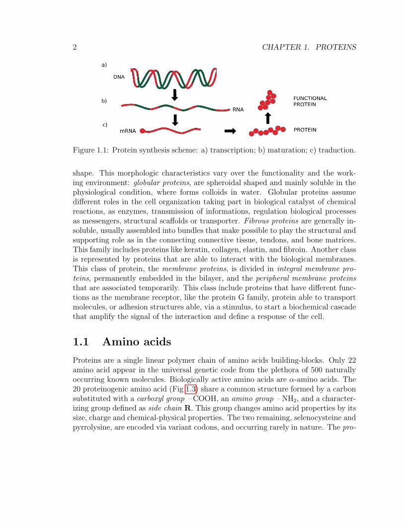
Proteins are the most common polymers in the biological world and, furthermore,these macromolecules exhibit huge diversity in function as a result of their variety inthree-dimensional structure and chemical activity. Chemico-physical distinctive fea-tures are given by the monomeric forming subunits: amino acids. Cells or metabol-ically inert structures, like viruses, genetic heritage are expressed with the purposeto build up the metabolic machinery which is mainly composed by proteins. Proteinare assembled in a specific amino acid sequence by the cell through transcription,maturation and traduction processes (Fig. 1.1). Transcription is the first step ofgene expression, in which a particular segment of DNA is transcripted and copiedinto RNA. Maturation process lead a full functional RNA from a precursor messen-ger RNA (pre-mRNA). DNA is responsible of storage of the biological informationwhereas RNA convey, specifically as mRNA, the genetic information to the protein.Translation, finally, is the process in which ribosomes decode the information codedin mRNA by the binding of complementary tRNA anticodon sequences to mRNAcodons. tRNAs, the RNA transfer, are specific RNA sequences, with an amino acidphysically binded in the structure, that works as adapter from the RNA codons codeto the amino acid sequences. Amino acids are chained together by the ribosomemachinery into a polypeptide and are released from the ribosome in the cell environ-ment where reach the mature conformation through the protein folding processes.Protein function arise from the specific three-dimensional structure defined by thisprocess. Depending on the length of the protein this process can be molecular drivenby molecular chaperones that are proteins capable to assist the covalent folding orunfolding of a single protein or the assembly and disassembly of multiple foldedprotein subunits.
Protein native state can be divided in different categories according to size and
1
2 CHAPTER 1. PROTEINS
Figure 1.1: Protein synthesis scheme: a) transcription; b) maturation; c) traduction.
shape. This morphologic characteristics vary over the functionality and the work-ing environment: globular proteins, are spheroidal shaped and mainly soluble in thephysiological condition, where forms colloids in water. Globular proteins assumedifferent roles in the cell organization taking part in biological catalyst of chemicalreactions, as enzymes, transmission of informations, regulation biological processesas messengers, structural scaffolds or transporter. Fibrous proteins are generally in-soluble, usually assembled into bundles that make possible to play the structural andsupporting role as in the connecting connective tissue, tendons, and bone matrices.This family includes proteins like keratin, collagen, elastin, and fibroin. Another classis represented by proteins that are able to interact with the biological membranes.This class of protein, the membrane proteins, is divided in integral membrane pro-teins, permanently embedded in the bilayer, and the peripheral membrane proteinsthat are associated temporarily. This class include proteins that have different func-tions as the membrane receptor, like the protein G family, protein able to transportmolecules, or adhesion structures able, via a stimulus, to start a biochemical cascadethat amplify the signal of the interaction and define a response of the cell.
1.1 Amino acids
Proteins are a single linear polymer chain of amino acids building-blocks. Only 22amino acid appear in the universal genetic code from the plethora of 500 naturallyoccurring known molecules. Biologically active amino acids are α-amino acids. The20 proteinogenic amino acid (Fig 1.3) share a common structure formed by a carbonsubstituted with a carboxyl group –COOH, an amino group –NH2, and a character-izing group defined as side chain R. This group changes amino acid properties by itssize, charge and chemical-physical properties. The two remaining, selenocysteine andpyrrolysine, are encoded via variant codons, and occurring rarely in nature. The pro-

1.1. AMINO ACIDS 3
Figure 1.2: Protein morphology: a) globular protein, caprine serum albumin(5ORI);b)Fibrous proteins, a collagen-like protein (1CAG); c) Memebrane protein, structureof serotonin receptor.
line amino acid have a peculiar structure as the side chain R bonds the amino groupforming a imino group. Side chains are mainly composed by other carbon atomsthat are nominated β, γ, δ, ε-carbon taking as reference the α-carbon. α-carbonis a chiral center because the tetrahedral configuration of the orbitals as well as,consequently, the bonds geometry, are substituted with four different groups, hence,molecules like amino acids are optically active and capable to rotate the plane ofpolarized light. The enatiomers are specified as Fisher’s convention for simple sugarsby the D,L system. In terms of a living system D and L stereoisomers are absolutelydifferent and, in almost universal way, the biologic amino acid are L stereoisomers.A particular case is carried by the glycine, since the side chain is composed by onlya hydrogen which makes this amino acid not chiral. The different chemical groups inthe amino acids side chains ensure three states: cationic, protoned or a zwitterionic.The zwitterionic state can be found when a molecule, with two or more functionalgroups, has a positive a negative electrical charge in different regions making the netcharge of the entire molecule zero. Under physiological conditions (pH 7) the mostcommon state is the zwitterionic, since the amine group deprotonates the carboxylacid via a kind of intramolecular acid–base reaction:
NH2RCHCO2H NH3+RCHCO2
–
Amino acid can be categorized in four groups: hydrophobic side chain, polar
4 CHAPTER 1. PROTEINS
uncharged side chain, electrically, positive or negative, charged side chain.
Hydrophobic side chain. The hydrophobic amino acids are glycine, alanine, va-line, leucine, isoleucine, methionine, proline, phenylalanine, and tyrosine. Note-worthy amino acids in this category are the proline, methionine and tyrosine.Proline is characterized by pyrrolidine side chain and it is the only amino acidwith a secondary amine bonded directly to amino group, making the α-carbona side chain atom. Due of the stiffness of this amino acid, proline is commonlyfound as the first residue of an α-helix, in the edge strands of β-sheets, andin turns structure of the proteins. Methionine, besidesthe polar unchargedcysteine, is one of two sulfur-containing amino acids. Tyrosine, despite thepresence of an hydroxyl group (–OH) can be considered partially hydrophobicbecause of the aromatic group that is significantly less soluble in water.
Polar uncharged side chain. These amino acid are the serine, threonine, tryp-tophan, cysteine, asparagine and glutamine. Serine and threonine have a hy-droxyl group (–OH), asparagine and glutamine an amidic group (–CONH2).Cysteine is characterized by a thiol group (–SH). This amino acid has a pivotalrole in protein structure since thiol group can be oxidated to give the disulfidederivative cystine.
Electrically positive charged side chain Amino acids in this category are ly-sine, arginine and histidine. These side chain ends with an aminic group, aguanidino group and a imidazole group, respectively. These end groups makethe side chain hydrophilic. The imidazole have a pKa of 6 and in physiologi-cal environment can be protoned or deprotonated in function of the chemicalmakeup.
Electrically negative charged side chain Aspartate and glutamate shares a car-boxyl (–COOH) common feature.

1.2. FORCES 5
Figure 1.3: The 20 proteinogenic amino acid. Image taken from [4].
1.2 Forces
Protein folding, peptide interaction, enzymatic activity are driven by a differentnon-trivial, considering the complexity of the protein chemical characteristics, inter-actions. The forces interplay in protein stability are prevalently non-covalents forces,with the exception of the sulfur bridges formed by cystine, the oxidized dimer formof the amino acid cysteine, that is covalent. These non-covalent interaction are thehydrogen bonds, the electrostatic interactions, and Van der Waals interactions.
Hydrogen bonds. The Hydrogen bond is an high directional electrostatic bondwhere an electronegative atom, like oxygen or nitrogen, is able to exert charge

6 CHAPTER 1. PROTEINS
delocalization on the bonded hydrogen making this positive. This positivepartial charge is able to bind an negative charged atom in the environment.This kind of bond plays a focal role in protein interaction and stabilization.The electronegative atom not covalently attached to the hydrogen is namedproton acceptor, instead the one covalently bound to the hydrogen is named theproton donor. This kind of bond is often described as an electrostatic dipole-dipole interaction. H-bonds share some features with covalent bond since it isdirectional and produces interatomic distances shorter than the sum of the vander Waals radii. Hydrogen bond is highly directional and, consequently, thestrongest interaction is due when the the acceptor is aligned to the covalentbond between the donor and the hydrogen atom. Because of this geometricfeature, a deviation from linearity leads to a decrease in energy of binding.Typical length of this kind of bonds is 2.5 A to 3 A. As explained later on, thepeptide hydrogen bonds are involved in the structure stabilization.
Electrostatic interaction. This force is generated between the charged or par-tially charged group, typical of the electrically charged amino acids, can bedescribed as a coulombian interaction between two point charges in a dielectricenvironment. Electronegativity cause delocalization of electron density towardsthe more electronegative atoms, generating a dipole moment able to interactelectrostatically.
van der Waals. Pairs of atoms interact with a van der Waals energy potential infunction of the distance r. The most common interaction potential employedis the in Lennard-Jones form
VLJ =C(12)
r12− C(6)
r6(1.1)
The first term, the repulsive one, is generated by the overlapping on the elec-tronic orbitals, that is, commonly, modeled as hard spheres with van der Waalsradius. This repulsive interaction is one of the main force that generate theconstraint interaction. Typical radius of carbon atom is 1.55 A, while, for ni-trogen is 1.75 A. When two atoms are covalently bonded the distance betweenthe center of the species is less the sum of radii. So Van der Waals radius of adefined element is relative to the bond co-partecipant.
1.3. PRIMARY STRUCTURE OF PROTEIN 7
Figure 1.4: Peptide bond condensation reaction. In highlighted are the peptide bond.
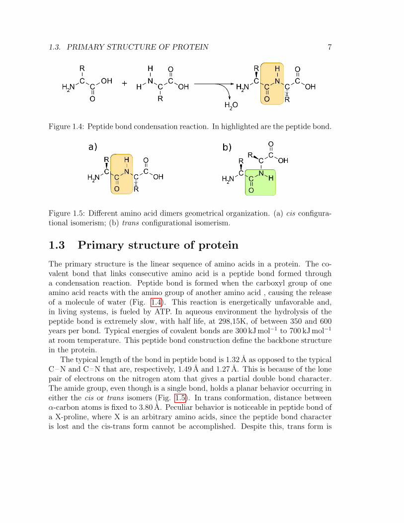
Figure 1.5: Different amino acid dimers geometrical organization. (a) cis configura-tional isomerism; (b) trans configurational isomerism.
1.3 Primary structure of protein
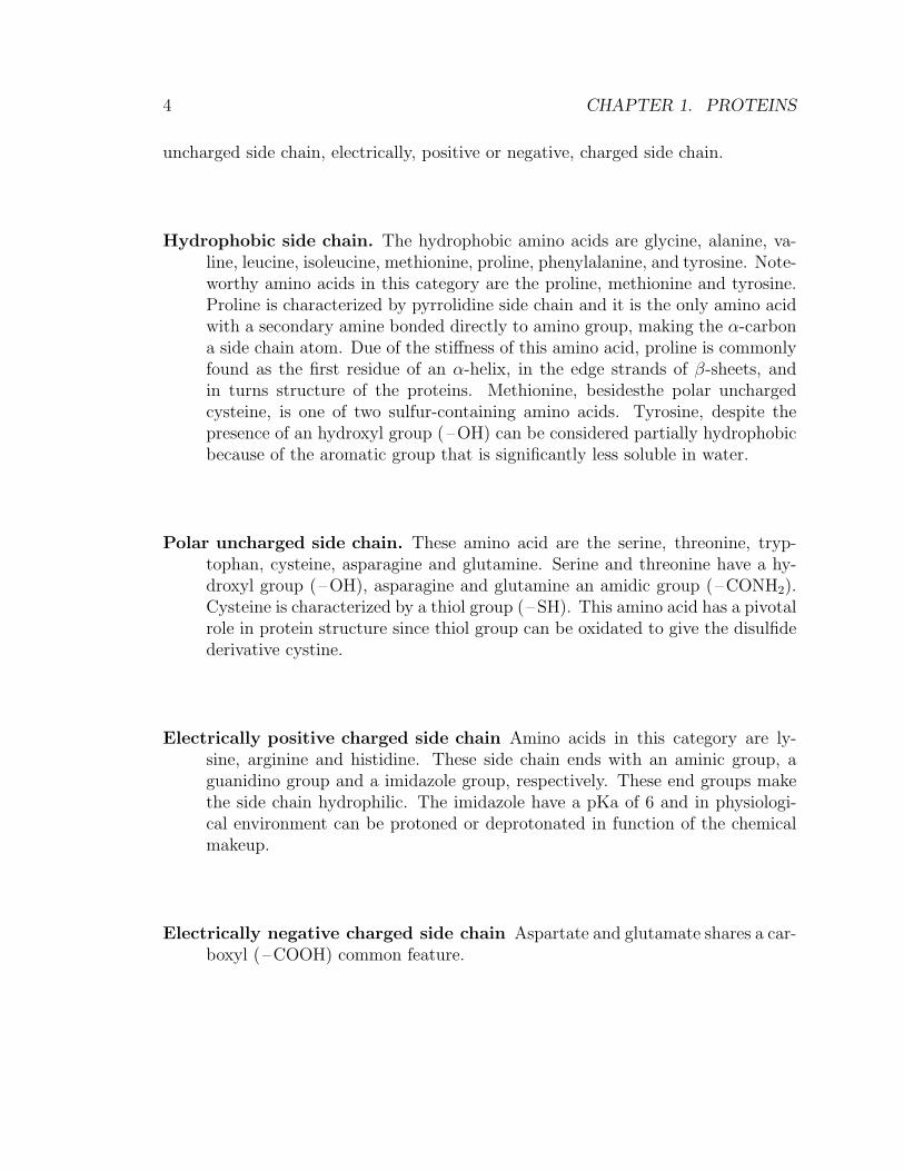
The primary structure is the linear sequence of amino acids in a protein. The co-valent bond that links consecutive amino acid is a peptide bond formed througha condensation reaction. Peptide bond is formed when the carboxyl group of oneamino acid reacts with the amino group of another amino acid , causing the releaseof a molecule of water (Fig. 1.4). This reaction is energetically unfavorable and,in living systems, is fueled by ATP. In aqueous environment the hydrolysis of thepeptide bond is extremely slow, with half life, at 298,15K, of between 350 and 600years per bond. Typical energies of covalent bonds are 300 kJ mol−1 to 700 kJ mol−1
at room temperature. This peptide bond construction define the backbone structurein the protein.
The typical length of the bond in peptide bond is 1.32 A as opposed to the typicalC–N and C––N that are, respectively, 1.49 A and 1.27 A. This is because of the lonepair of electrons on the nitrogen atom that gives a partial double bond character.The amide group, even though is a single bond, holds a planar behavior occurring ineither the cis or trans isomers (Fig. 1.5). In trans conformation, distance betweenα-carbon atoms is fixed to 3.80 A. Peculiar behavior is noticeable in peptide bond ofa X-proline, where X is an arbitrary amino acids, since the peptide bond characteris lost and the cis-trans form cannot be accomplished. Despite this, trans form is
8 CHAPTER 1. PROTEINS
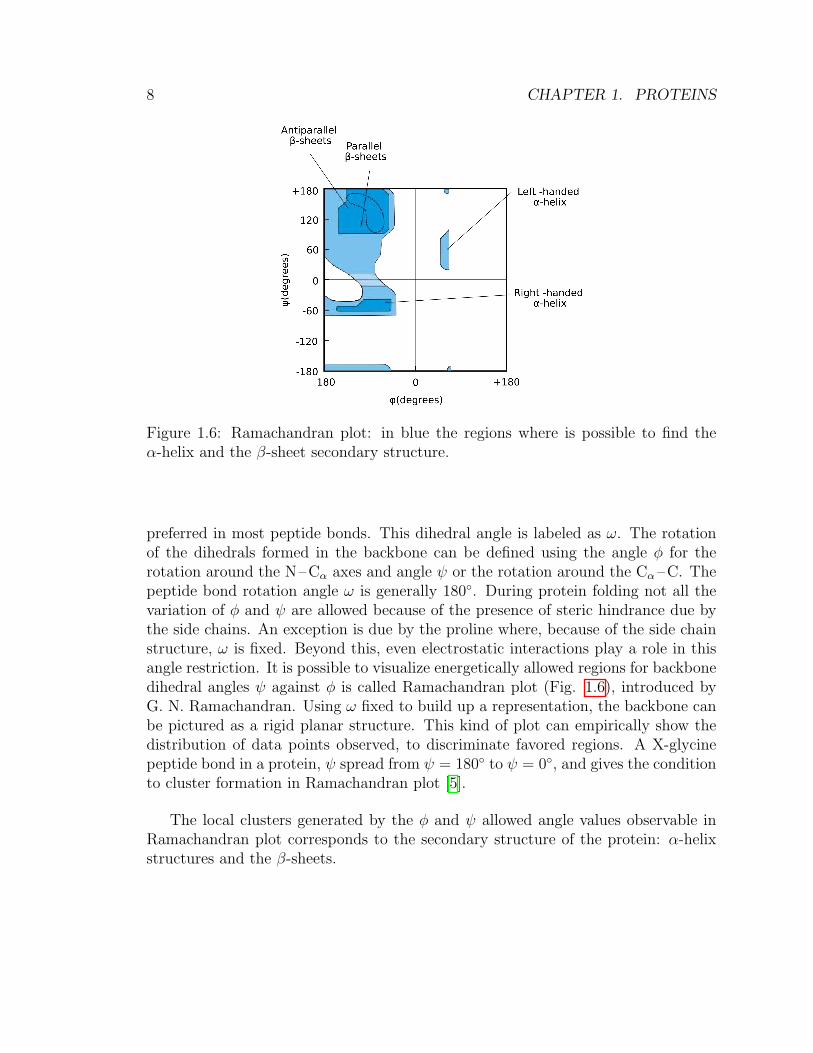
Figure 1.6: Ramachandran plot: in blue the regions where is possible to find theα-helix and the β-sheet secondary structure.
preferred in most peptide bonds. This dihedral angle is labeled as ω. The rotationof the dihedrals formed in the backbone can be defined using the angle φ for therotation around the N–Cα axes and angle ψ or the rotation around the Cα –C. Thepeptide bond rotation angle ω is generally 180◦. During protein folding not all thevariation of φ and ψ are allowed because of the presence of steric hindrance due bythe side chains. An exception is due by the proline where, because of the side chainstructure, ω is fixed. Beyond this, even electrostatic interactions play a role in thisangle restriction. It is possible to visualize energetically allowed regions for backbonedihedral angles ψ against φ is called Ramachandran plot (Fig. 1.6), introduced byG. N. Ramachandran. Using ω fixed to build up a representation, the backbone canbe pictured as a rigid planar structure. This kind of plot can empirically show thedistribution of data points observed, to discriminate favored regions. A X-glycinepeptide bond in a protein, ψ spread from ψ = 180◦ to ψ = 0◦, and gives the conditionto cluster formation in Ramachandran plot [5].
The local clusters generated by the φ and ψ allowed angle values observable inRamachandran plot corresponds to the secondary structure of the protein: α-helixstructures and the β-sheets.

1.4. SECONDARY STRUCTURE OF PROTEIN 9
1.4 Secondary structure of protein
Local conformation as a consequence of protein folding are referred as secondarystructure. This kind of organizations are particularly stables and are a peculiarityof protein structure. Secondary structure are stabilized by the H-bond formationbetween the H-bond donor and acceptor species in the backbone, since hydrogenatom in the secondary amine group –R2NH is partially positive charged by theelectronegativity of the nitrogen atom, and chemical groups like the carbonyl –C––Ocan form two non-linear H-bonds with the covalent bond. The most importantsecondary structures are the α-helix and the β-sheet. Other structure, like β-turnor ω-loop, are stabilized by this kind of interaction but play a minor role in protein.Pioneering works in protein analysis has been made by Pauling e Corey that predictedthe secondary structure from the optimization of H-bond in proteins [6] , and byRamachandran that studied the sterically accepted torsion angle in proteins secondstructures formation.
1.4.1 α-helix
The α-helix (Fig. 1.7(a)) is the simplest arrangement in which a protein can occurduring protein folding. This is due for the optimal use of H-bonds between thenitrogen atom and the carbonyl oxygen, located on the fourth amino amino acidaway (i + 4 → i H-bonds). α-helix backbone proceeding recall a coil springs or thehandrails of spiral staircases, side chains in this representation go outwards respectof the central pole. Each turn of the helix extend the total length of the helix of5.4 A using 3.6 amino acids. The φ and ψ variates of −45◦ to −50◦ and −60◦,respectively, forming prevalently right-handed structures. Mixed stereoisomers arenot able to form α-helix structures. The former simplified model of α-helix hasbeen build without take into account the effect of the side chain steric hindrance orcharged species that not promote the structure formation. For instance, if a proteinhas a secondary structure formed by a sequence of amino acid belonging to thesame electrically charged side chain family, α-helix will be not built up because ofthe electrostatic interaction between these side chains. Branched amino acids likevaline, isoleucine and threonine destabilize this structure the for steric interaction.Amino acids that are able to form H-bonds can interact with the backbone and,subsequently, unpromote the α-helix formation. As precedently explained, proline,if involved in a peptide bond, due is peculiar side chain structure, is not able toform H-bonds, since the secondary amine, canonically present in the backbone, is atertiary amine –R3N.
10 CHAPTER 1. PROTEINS
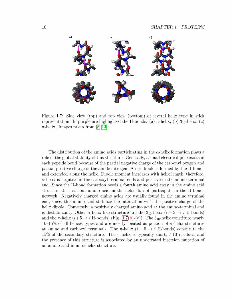
Figure 1.7: Side view (top) and top view (bottom) of several helix type in stickrepresentation. In purple are highlighted the H-bonds: (a) α-helix; (b) 310-helix; (c)π-helix. Images taken from [8–13].
The distribution of the amino acids participating in the α-helix formation plays arole in the global stability of this structure. Generally, a small electric dipole exists ineach peptide bond because of the partial negative charge of the carbonyl oxygen andpartial positive charge of the amide nitrogen. A net dipole is formed by the H-bondsand extended along the helix. Dipole moment increases with helix length, therefore,α-helix is negative in the carboxyl-terminal ends and positive in the amino-terminalend. Since the H-bond formation needs a fourth amino acid away in the amino acidstructure the last four amino acid in the helix do not participate in the H-bondsnetwork. Negatively charged amino acids are usually found in the amino terminalend, since, this amino acid stabilize the interaction with the positive charge of thehelix dipole. Conversely, a positively charged amino acid at the amino-terminal endis destabilizing. Other α-helix like structure are the 310-helix (i + 3 → i H-bonds)and the π-helix (i+5→ i H-bonds) (Fig. 1.7(b)-(c)). The 310-helix constitute nearly10–15% of all helices types and are mostly located as portion of α-helix structuresat amino and carboxyl terminals. The π-helix (i + 5 → i H-bonds) constitute the15% of the secondary structure. The π-helix is typically short, 7-10 residues, andthe presence of this structure is associated by an underrated insertion mutation ofan amino acid in an α-helix structure.
1.4. SECONDARY STRUCTURE OF PROTEIN 11
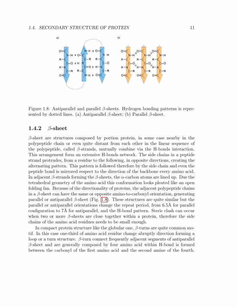
Figure 1.8: Antiparallel and parallel β-sheets. Hydrogen bonding patterns is repre-sented by dotted lines. (a) Antiparallel β-sheet; (b) Parallel β-sheet.
1.4.2 β-sheet
β-sheet are structures composed by portion protein, in some case nearby in thepolypeptide chain or even quite distant from each other in the linear sequence ofthe polypeptide, called β-strands, mutually combine via the H-bonds interaction.This arrangement form an extensive H-bonds network. The side chains in a peptidestrand protrudes, from a residue to the following, in opposite directions, creating thealternating pattern. This pattern is followed therefore by the side chain and even thepeptide bond is mirrored respect to the direction of the backbone every amino acid.In adjacent β-strands forming the β-sheets, the α-carbon atoms are lined up. Due thetetrahedral geometry of the amino acid this conformation looks pleated like an openfolding fan. Because of the directionality of proteins, the adjacent polypeptide chainsin a β-sheet can have the same or opposite amino-to-carboxyl orientation, generatingparallel or antiparallel β-sheet (Fig. 1.8). These structures are quite similar but theparallel or antiparallel orientations change the repeat period, from 6.5A for parallelconfiguration to 7A for antiparallel, and the H-bond pattern. Steric clash can occurwhen two or more β-sheets are close together within a protein, therefore the sidechains of the amino acid residues needs to be small enough.
In compact protein structure like the globular one, β-turns are quite common mo-tif. In this case one-third of amino acid residue change abruptly direction forming aloop or a turn structure. β-turn connect frequently adjacent segments of antiparallelβ-sheet and are generally composed by four amino acid within H-bond is formedbetween the carbonyl of the first amino acid and the second amine of the fourth.

12 CHAPTER 1. PROTEINS
Figure 1.9: Different secondary structures: (a) β-barrel; (b) β-α-β; (c) α-α corner.
Glycine and proline usually take parts in β-turns for different function: glycine issmall and flexible, proline, instead, for the peculiarity of the amino acid structure,forces backbone to assume a cis configuration which permit a tight turn. Consider-ably less common is the γ-turn, a three residue turn with a hydrogen bond betweenthe first and third residues.
1.5 Tertiary and quaternary structure
The arrangement of several secondary structures are called supersecondary struc-tures, also called folds or motifs (Fig. 1.9). This complex structures cluster sharessimilar function in different proteins. Protein with more than 300-400 amino acidfolds in specific globular sub-regions called domains. This subdivision arise by anevolutionary advantage given by the quicker folding and the possibilities of each do-main to fold individually. Domains can be characterized by the fold. Domains havethe same fold if can share similar supersecondary structures.
The tertiary structure represent the three-dimensional shape of a proteins, whereasthe arrangement of a protein composed from different polypeptide chains is definedas quaternary structure. In this hierarchic level, same multiple sub-unit can interactand, usually, are arranged with rotational or helical symmetry. This kind of sub-units super structures are preferred, in evolutionist terms, because built up a fullyfunctional multi-polypeptide protein can lead to translations error or misfoldings.Further than this, use single chain protein to build up complex structure is moreefficient from a genetic heritage usage since the information for each sub-unit needto be stored just one time.
1.6. PROTEIN FOLDING 13
Protein can be classified by the The Structural Classification of Proteins (SCOP)database. The hierarchical organization is defined as, follows
Class Type of folds.
Fold The different three dimension structure of domains in a class.
Superfamily Domain in a fold grouped in superfamilies, which have a distant com-mon ancestor.
Family Domain in a superfamily grouped in families, which have a recent commonancestor.
Protein Domain Domain in a fold grouped in protein domains, same protein.
Species Domain in protein domain grouped in species
Domains Part of a protein, for small proteins can be the whole one.
The classes groups the domains eleven categories depending on the second struc-ture contents, type of protein, or quality. Four on eleven are dedicated for the secondstructure content: all-α proteins are composed prevalently by α-helix, all-β, contro-versially, are defined by the prevalence of β-strands, α/β include β − α − β whereβ-sheets are surrounded by α-helices. Last category is α+ β where no evident motifarise.
1.6 Protein folding
The three-dimensional unique structure in which a protein can fold is defined by theinteraction of a specific polypeptide sequence and environment contribute. In thelast decades many works tried to clarify this process, using both experimental andtheoretical approaches, in order to reveal the intimate interplays from which arise adefined native state. Protein folding structure prediction as the Chou-Fasman [14]or the Garnier-Osguthorpe-Robson [15] methods, focus on this kind of possibility.The knowledge of the physical connection between a defined primary sequence andthe final geometrical configuration have not only basic knowledge purpose but evenstrictly practical. Genetic engineering has been involved the modification of naturallyoccurring proteins and the ability to manage the protein folding precess should be apossible way to design new functional proteins that can be used in pharmacological,industrial and general nanotechnology field. Bioinformatics use data bases of protein

14 CHAPTER 1. PROTEINS
Figure 1.10: General proceedings of an enzymatic activity as function of temperature.
structures and relative amino acids or nucleotide sequences to find , using a statisticalapproach able to identify similarities, a possible structure, function or, from a geneticspoint of view, a phylogenetic path to a common ancestor.
The understanding of the denaturarion, the loss of three-dimensional structureand function, and renaturation has been a starting point for the thermo analyticalprotein studies. Protein structure evolved to have a specific function and activityin a well defined cellular environment, due the definition of denatured state, emergethat a precise polypeptide could cover different paths of folding in function of theinteracting solvent. Denatured state is non unique and is better described as a familyof structure that occur in a random linear configuration and in a, subsequently, lossof function. Since the folded state is defined by a complex interplay due by weakinteraction, provide heat to the system can be one of the way to denature a protein.If the change in temperature is controlled and is increased slowly, protein functionand structure remains stable until an a sudden loss of activity. This sigmoid-shapedchange (Fig. 1.10) implies that a small lost in structure stability destabilize the otherparts.
The tertiary structure is determinate, as the secondary, by the amino acid se-quences. This statement can be proved because denaturation, as shown by someexperiments, can be reversible. This process is called renaturation. First evidencethat the amino acid sequence holds all the information necessary for the folding wascarried out by Anfinsen in the 1950s [16]. This shows that protein folding is a ther-modynamically driven processes where the ground state of this system is the nativestructure and the solvent molecules. The reversibility of unfolding and refolding,using thermodynamic stability, is a two-state process:
P (Fold) ku−⇀↽− P (Unfold) (1.2)
The reversibility observed by the Anfinsen experiment is enshrined in this type of two

1.6. PROTEIN FOLDING 15
Figure 1.11: Different types of energy landscape. On the left an ideal funnel shapedenergy landscape. On the right a frustrated system, characterized by many localminima.
step process. Purified ribonuclase, a type of nuclease that catalyzes the degradationof RNA into smaller components, can be denatured in urea solution in the presenceof 2-mercaptoethanol as reducing agent. This molecule is able to reduce the disulfidebond, meanwhile urea minimize the hydrophobic interaction pushing structure tounfold. After the removal of urea and 2-mercaptoethanol, protein refolds in theactive native structure. If the process was random the eight cysteine could recombineto build up the four disulfide bonds in 105 different ways.
Proteins generated by the metabolic machinery are assembled in a very high rate.A complete, biologically functional protein of 100 amino acids can be synthesized inroughly 5 second at 37 ◦C. This 100 residues protein have 99 bonds and 198 possibleφ and ψ angle value. Hypnotizing, that only three configuration are accepted bya random process and each possible conformation is tested until it finds the nativestate this require 3198 steps. Assuming the shortest possible time (≈10× 10−13 sec)for bond rotation, the time required for the process would amount 1072 years, morethat the age hypotized for the universe (13.8× 10⁹ years). This statement, calledLevinthal’s paradox, was proposed by Cyrus Levinthal to point out that proteinfolding cannot be a random process [17]. Many models has been proposed to elu-cidate this process [24–26]. In all of them he common feature lies in the Principleof minimal frustration proposed by Joseph Bryngelson and Peter Wolynes in the’90s [21]. The energy landscape, a representation of energy function across the con-figuration space of the system, of a protein is generally coarse, so a change in the

16 CHAPTER 1. PROTEINS
conformation define a jumpy and many minima profile in energy, generating multi-ple u-shaped energetic wells directed to the minimum (Fig. 1.11). This roughnessof the energy landscape generate in a many interaction in energy function. Thisinteraction is defined frustation. A canonical example of frustrated system is thespin glass [18], a disordered magnetic system in which spins of the component atomsare randomly directed. The analogy with glass arise from the disorder position pfthe magnetic component as bonds in an amorphous solid. Spins in this kind of sys-tem interact as consequence of the random position, pointing in the same direction(ferromagnetic) or in opposite direction (anti-ferromagnetic). These local behavioris not able to satisfy completely a spin general arrangement of the system that is,consequently, frustrated. Complex systems, like protein folding need to be describedadding a stochastic component to the Hamiltonian and gaining the system fuzziness.Frustration, in polymers, arise from the inability to satisfy electrostatic interactiondue the unfavorable path needed to this hypothetical optimization since the systemcannot satisfy all the energetic and geometrical constraint simultaneously.
The principle of minimal frustration has been stated to solve this discrepancies.The idea of this principle defines that evolution selected that amino acid sequenceables to fold in a stable and functional form. In parallel, evolution, operates acounter-selection against the amino acids that disfavored an appropriated folding.Richard Dawkins in ”The Blind Watchmaker” wrote: “Mutation is random; naturalselection is the very opposite of random ” [22]. Nature uses mutation as materialfor change, and even in the principle of minimal frustration changes are feasible aslocal minima in the energy landscape of protein folding. Jose Onuchic proposedthat protein folding energy landscape are funnel like, with local minima but strictlydirected in a global minimum or ground state where lies the native protein [23].Three-dimensional energy landscape consist in the configuration space of the protein(x, y) and the energy (z). At higher energy system, near the upper-edge of the funnel-shaped potential, as reported in Fig. 1.12, the correlated configuration space, theprotein is unfolded and reach the maximum number of conformation, indicating thatthe unfolded state is a family of possible configuration that converge with differentpath of folding in a unique native configuration. If the denatured state were a uniqueconfiguration the energy landscape, using a geographical analogy, should be on theon the tip of a high ground. These pathways can be used more or less frequentlydepending the thermodynamic favorability. During the intermediate state, or moltenglobule, protein starts to assume more thermodynamically favorable structure untildo not attain the native state [28]. The funneled energy landscape and the principleof minimal frustration are consequences defined by a ”top-down” approach for theprotein folding.

1.7. PROTEIN SOLUBILITY AND STABILITY 17
Figure 1.12: The energy folding funnel landscape for protein denaturation. Thewidth of funnel is related with the entropy of the system.
In literature the two most supported models are the hierarchical [34] and the HPmodel [26]. In the hierarchical model, local second structure are the first structureformed by the primary sequences since some amino acid fold more specifically in α-helix or β-sheets. Supersecondary structure are built up subsequently by long-rangeinteraction of the former. This process continues until complete folding. Anothermodel, HP model, states that protein collapse due the cooperation of hydrophobicinteraction with aqueous environment, taking in to account only the difference be-tween hydrophobic (H) and polar (P) amino acid residues. The interaction energybetween two hydrophobic amino acids VHH is negative, instead interaction betweentwo polar amino acids VHP or mixed types VPP a larger energy. The HP model hasbeen used as interacting parameter in lattice protein simulation, where interactionof hydrophobic residues are the driving force of protein folding using an explicit kindof solvent.
1.7 Protein solubility and stability
The solubility of proteins is correlated with the distribution of hydrophilic and hy-drophobic amino acids in the protein surface. Globular protein carry out function

18 CHAPTER 1. PROTEINS
Figure 1.13: Interface double layer diagram showing the electrolyte concentration anpotential as function of distance from the charged surface.
in aqueous environment and, consequently, hydrophilic residues occur prevalently inthe protein surface. Protein with high presence of hydrophobic amino acids have lowsolubility in water and prefer to bind or be completely surrounded by polar envi-ronment. Trans-membrane proteins are an example of this case, since are partiallyor totally immersed in the phospholipidic bilayer. Charged surface interaction withsolvent is fundamental for protein activity since solvation shell around the protein(≈10 A) have a completely different behavior respect the bulk. When proteins aresolubilized in physiological environment the electrolyte couterions associate to theproteins surface forming a shell, named as Stern layer (Fig. 1.13). Next to thisshell water molecules form a solvation layer able to diffuse from the shell to the bulksolvent with a gradient that contains a decreasing contraction of couterions and anincreasing concentration of ions. The thickness of this layer is called Debye lengthand the outer layer is the diffuse layer. The Debye layer is characterized by thepresence of a slipping plane that separates mobile fluid from fluid that remains at-tached to the surface. On this plane the electric potential, the ζ-potential, can besee as the potential between solvent and dispersed protein. The precedence of thislayers decrease the aggregation because of the decrease in ionic interactions. The ζ-potential is used as indicator of the colloidal stability of a solution. This description
1.7. PROTEIN SOLUBILITY AND STABILITY 19
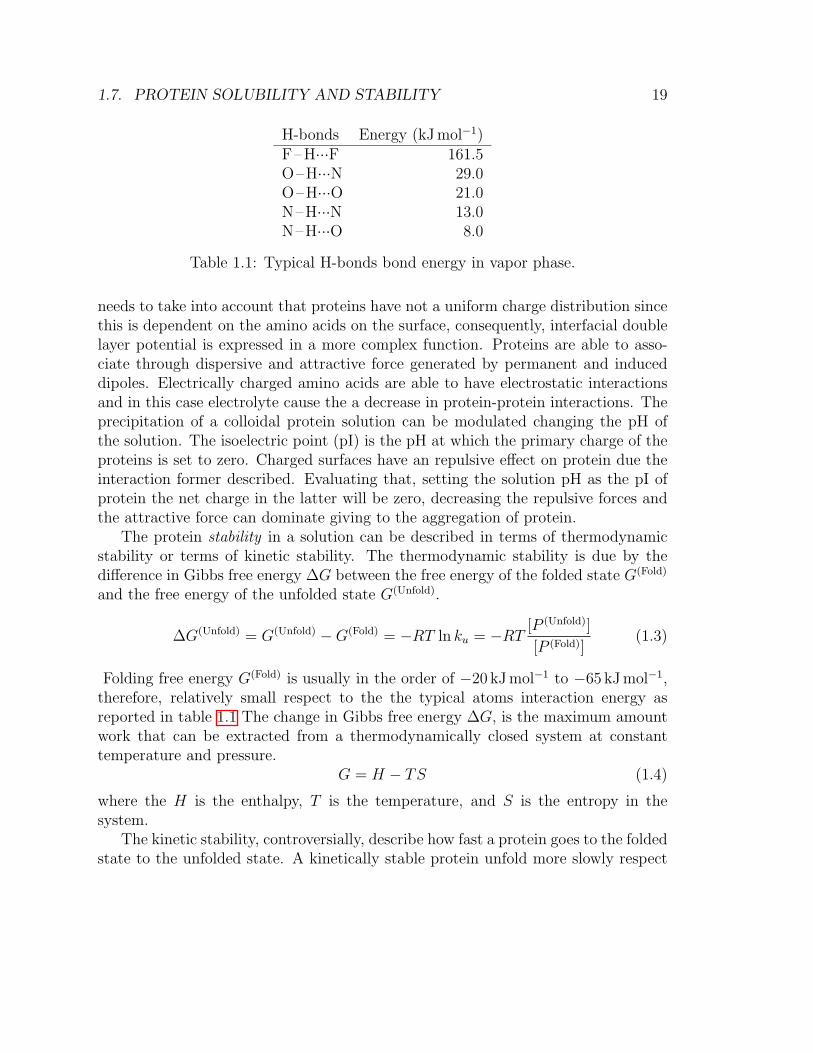
H-bonds Energy (kJ mol−1)F–H···F 161.5O–H···N 29.0O–H···O 21.0N–H···N 13.0N–H···O 8.0
Table 1.1: Typical H-bonds bond energy in vapor phase.
needs to take into account that proteins have not a uniform charge distribution sincethis is dependent on the amino acids on the surface, consequently, interfacial doublelayer potential is expressed in a more complex function. Proteins are able to asso-ciate through dispersive and attractive force generated by permanent and induceddipoles. Electrically charged amino acids are able to have electrostatic interactionsand in this case electrolyte cause the a decrease in protein-protein interactions. Theprecipitation of a colloidal protein solution can be modulated changing the pH ofthe solution. The isoelectric point (pI) is the pH at which the primary charge of theproteins is set to zero. Charged surfaces have an repulsive effect on protein due theinteraction former described. Evaluating that, setting the solution pH as the pI ofprotein the net charge in the latter will be zero, decreasing the repulsive forces andthe attractive force can dominate giving to the aggregation of protein.
The protein stability in a solution can be described in terms of thermodynamicstability or terms of kinetic stability. The thermodynamic stability is due by thedifference in Gibbs free energy ∆G between the free energy of the folded state G(Fold)
and the free energy of the unfolded state G(Unfold).
∆G(Unfold) = G(Unfold) −G(Fold) = −RT ln ku = −RT [P (Unfold)]
[P (Fold)](1.3)
Folding free energy G(Fold) is usually in the order of −20 kJ mol−1 to −65 kJ mol−1,therefore, relatively small respect to the the typical atoms interaction energy asreported in table 1.1 The change in Gibbs free energy ∆G, is the maximum amountwork that can be extracted from a thermodynamically closed system at constanttemperature and pressure.
G = H − TS (1.4)
where the H is the enthalpy, T is the temperature, and S is the entropy in thesystem.
The kinetic stability, controversially, describe how fast a protein goes to the foldedstate to the unfolded state. A kinetically stable protein unfold more slowly respect

20 CHAPTER 1. PROTEINS
to a kinetically not stable one. This case is not an equilibrium process since theprotein unfold to a denatured state in irreversibly way. The energy needed for theunfolding process from the kinetic point of view is the amount of energy necessaryto pass from the folded state to the transition point. This energy is well knows asthe activation energy. The irreversible unfolding is described by the relation:
P (Fold) ku−⇀↽− P (Unfold) ki−⇀ P (Inactive) (1.5)
where the energies barrier to the inactivated state P (Inactive) is smaller the the acti-vation energy needed the transition point to the folded state P (Fold).
The main contributions to protein stability, most widely accepted in literature, arethe hydrogen bonds and the hydrophobic effect. These contributions are cooperativesince iteration generated by each residue are generally small. On the other hand, theunfolded state is stabilized by the conformational entropy. The rotation of a bondin denaturated state is much more favorite then in folded state. This define a strongentropic driving force for unfolding. Conformational entropy can be figured, likewise,as that increasing the stiffness of a polypeptide in the unfolded state, decreasing thepossible configuration in the unfolded state, implies in a stability gain for the foldedstare respect on the unfolded state [30]. Therefore, the unfolded protein is a limit casewhere all the residue interact only with the water molecules and do not interact asintra-protein bonds. Using this definition the unfolded state is, in opposite way to thefolded state in a given solvent, a collection of extended conformations. This pictureis not able to fit always the experiment evidence. Rarely, unusual behavior has beenreported in literature [31]. For the present aim, we assume that all interaction thatstabilize the native state, i.e the H-bonds, are completely removed in unfolded state.
As previously described the H-bonds have a noteworthy role protein folding. Be-yond the peptide hydrogen bond, H-bonds behavior of liquid water, and the globaluniqueness respect to other liquid, take a relevant contribute. In a water molecule,using oxygen as reference, there are four regions of excess of charge in tetrahedralarrangement. Two on four are generated by the hydrogen atoms due the high elec-tronegativity of the oxygen that attract the shared pair of electrons towards itself.The negative excess of charge, otherwise, is located in two ion-pairs on the oxygen.This charge disposal and the electronegativity of the oxygen make the H-bonds themain interaction between water molecules. The lowest arrangement is reach whenthe donor molecule, respect of the hydrogen-oxygen axis, is tilted of 57◦ on the or-thogonal plane to the plane of the hydrogen-oxygen-hydrogen of the acceptor [33].Taking into account a water molecule this generates four H-bond interaction withthe four nearby water molecule disposed in a tetrahedral arrangement. This dynamic

1.7. PROTEIN SOLUBILITY AND STABILITY 21
Figure 1.14: The tetrahedral arrangement of the liquid water.
configuration, where hydrogen atoms behave like donor and the ion-pairs as accep-tors, is called Walrafen pentamer. Since that, is possible to fill the space tessellationwith tetrahedral cells making the water capable to build a crystal typical of the solidice.
The H-bonds generated interaction in liquid water can be outlined by clusteringmodels where different number of water molecules interact in non canonical idealtetrahedral configuration. As reported in table 1.1 the strength of an hydrogenbonds is 8 kJ mol−1 to 29 kJ mol−1. Considering protein, McDonald at al. in 1994showed that for high resolution structure, buried nitrogen and oxygen atoms failfor the 9.5% and 5.8%, respectively, to form a H-bond but, relaxing the proteinstructure, roughly the 1-2% of the backbone H-bond donors and acceptors fails tobonds with the counterpart. Carbonyl, more specifically, fails with 80% the secondH-bond. [32] From an entalpic point of view the H-bonds contribute is unfavorablefor protein folding. Hydrogen bonds, instead, stabilize protein with an entropic effectdue by the disrupted H-bonds in water bulk by the presence of the protein, leadingan entropy gain in solvent.
The main driving force for protein folding as been conferred the to hydrophobiceffect proposed by Kauzmann et al (1959) but, recently, literature rebalanced thiscontribute significance [35]. The hydrophobic effect is given by the aggregation ofnonpolar substances in aqueous solution in order to not interact with water molecules.

22 CHAPTER 1. PROTEINS
This behavior characteristic of mixed nonpolar/aqueous solution is lead by H-bondsformation between molecules of water in the way to minimizes the area of contactbetween water and nonpolar molecules. This interaction is typical in aqueous envi-ronment since dipole-dipole interaction in water are stronger than the dipole-inducedbetween water and protein. From a general point of view, in a multi-phase solventthe energy needed to transfer a non-polar molecule from an organic phase to polarone is the energy of transfer ∆G
(Polar)Tr
∆G(Polar)Tr = ∆H
(Polar)Tr − T∆S
(Polar)Tr (1.6)
In normal condition of temperature (300 K), the enthalpy of transfer ∆H(Polar)Tr is
negligible. Entropy, in contrast, is negative since water molecules interact, with H-bonds, with other water molecules. Locally, water nearby the non-polar compoundform H-bonds with subsequent lose of energy. Consequently, water balance loseenergy due the generation of water-water H-bonds near the solute molecule wherewater-water H-bonds pattern is similar to that of solid water. Rising the temperatureup to the boiling point of water, tetrahedral configurations are disrupted and, by therelation of entropy with the temperature, the entropy of transfer ∆S
(Polar)Tr tends to
zero. At the same time the enthalpy of transfer ∆H(Polar)Tr is positive. Even enthalpy
is correlated with the temperature by the Kirchoff’s Law. Enthalpy increase withtemperature, leading to a gain in enthalpies of product and reactants. At constanttemperature, the heat capacity is
Cp =
(∆H
∆T
)(1.7)
Kirchoff’s Law can be used only for small temperature change (±100 K) since forgreater range the correlation the heat capacity began not constant. In this lowerrange of temperature, the enthalpy change is proportional to the product of thechange in temperature and the variation in heat capacity for product and reactants.The final enthalpy is defined as
HTf = HTi =
∫ Tf
Ti
dTCp (1.8)
or for systems where the heat capacity is temperature independent for a definedrange of temperature:
HTf = HTi = cp(Tf − Ti) (1.9)
from the 1.7 is evident that the entropy and the enthalpy are temperature correlatedin different ratio. Because of this temperature correlation can be defined a specific

1.8. PROTEIN STABILITY IN SOLVENT OTHER THAN WATER 23
temperature in which the hydrophobic effect reach an optimum point and belowand above this temperature the hydrophobic effect decreases. Another result of thiswater lattice reorganization caused by the hydrophobic effect is the gain in thermalcapacity a result of protein unfolding, calorimetry routines (see A.2) use this variationto calculate the free energy. In spite of this, apolar side chain can be found inside theglobular structure of the proteins where mutually interact to contribute for proteinfolding. In protein folding this separation leads to a compact structure where apolarside chains are buried inside the globular structure to avoid the interaction withwater. Most recent theory compare the hydrophobic effect with the hydrogen bondsand the van der Waals interaction. The burial of a –CH2 – contributes ≈5.0 kJ mol−1
to the stability instead the ∆G(Polar)Tr is ≈4.0 kJ mol−1, suggesting that the 80% of the
hydrophobic effect is generated by the hydrophobicity and the 20% from the packingof amino acid side chain inside the globular structure [36].
Other minor factor are the charge-charge interactions, salt bridges, the aromaticstacking, metal binding and disulfide bonds. The distribution of charge in a proteinsurface, at physiological pH, arise to be more attractive than repulsive, so this in-teraction stabilize the folded state. Charge-charge interactions, on the other handtend to stabilize even the denaturated state making this contribution small. Charge-charge interactions have a dependence with the temperature and thermophilic or-ganisms seems to adopt this strategy to stabilize proteins [37]. The salt bridges area particular type of H-bonds strengthened by the combined effect of an electrostaticinteraction, typical the electrically charged amino acid positioned at less then 5 Aas glutamate and lysine. This interactions contribute less than ≈5 kJ mol−1 on theprotein surface. On the other hand, buried salt bridges have a contribute more than≈17 kJ mol−1.
Aromatic side chains as phenylalanine, tyrosine and tryptophan participate tothe protein stability with the aromatic stacking. This non-covalent interaction ispresented between the aromatic rings. The aromatic rings have more p-orbitalsdue by the covalent bonds, the superposition of these orbitals generate a so calledπ-orbital conjugated. The interaction of more π-orbital in stacked configurationstrengthen this bond more stable since there is a gain in shared electron.
1.8 Protein stability in solvent other than water
As precedently reported protein stability is in range of the order of 20 kJ mol−1 to65 kJ mol−1. Biological evolution use random mutations as bifurcation point for apossible more efficient, in some task point of view, product. This idea of evolution canbe observed in different complexity level as species, organism or molecules. Proteins

24 CHAPTER 1. PROTEINS
perform a widely array of function, from the structural protein, to the catalysis,passing through stocking, transport, receptor and so forth. All this classes have incommon the capability of interaction with other molecules by a particular moiety ofthe protein as a catalytic or a binding site. This interaction is strictly correlated withthe structure of the protein and the working environment: water. The evolutionarypressure for a protein needs to be well balanced between the functional state and thepossibilities to not accumulate a mutation with a prominent impact for the biologicalfunction. In general, a mutation that leads to a production of a damage for the nativeprotein stability is less probable than a decrease in stability. The low range energyin protein stability is used to control this type of event and prevent the accumulationof lethal mutation. Mutations can effect in different ways considering the amino acidsubstituted, in fact , mutations in amino acid that have similar chemico-physicalproperties, compared with the wild-type amino acid, have less influence on a largechange in stability. Stability can be used as different point of view of the functionality,since these two features are superimposed by the structure in native state. Mutationcan lead to misfolding, aggregation with other proteins, or non interaction with theproposal molecule.
During the folding process, protein lose entropy (∆Sprot < 0) meanwhile solventgains entropy (∆Ssolv > 0). Throughout this process protein break protein-water(P-W) H-bonds to form protein intramolecular (P-P) H-bonds. In parallel, waterbreak water-protein(W-P) H-bonds formed to restore the water tetrahedral H-bondsnetwork. In this case, the global balance of the components is not clear and cannotbe defined in advance. The H-bonds binding energy is defined by the reaction en-vironment. Another contribute is due by the electrostatic interaction, generated, inphysiological environment by electrically, positive or negative, charged side chains.This interaction are well defined in water environment. When a protein in trans-ferred in another solvent, as ethanol, cycloehexane or vacuum, all the interactionprecedently described needs to be re described, Pace in a 2004 work, described thiskind of interactions [38].
In this new solvent the native state needs to share the same features of the nativestate in water, so, must be favored as in water and the conformational stabilityneeds to be in in range of the order of 20 kJ mol−1 to 65 kJ mol−1. In the otherhand, each state, the unfolded and the folded, needs to be soluble in the new solvent.Ethanol (C2H6O) is completely miscible in water, polar organic solvent, aliphatichydrocarbons, and aliphatic chlorides. This molecule have a dipole moment (1.69 D)making this molecule polar. The presence of the hydroxyl group (–OH) able tomake H-bonds, permit to the ethanol to be less volatile than similar molecular weightcompound as the propane (C3H8). Controversially the cyclohexane (C6H12) is non
1.8. PROTEIN STABILITY IN SOLVENT OTHER THAN WATER 25
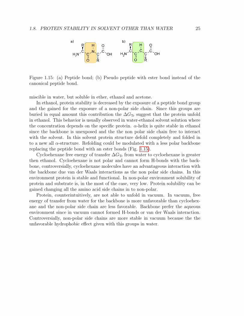
Figure 1.15: (a) Peptide bond; (b) Pseudo peptide with ester bond instead of thecanonical peptide bond.
miscible in water, but soluble in ether, ethanol and acetone.In ethanol, protein stability is decreased by the exposure of a peptide bond group
and the gained for the exposure of a non-polar side chain. Since this groups areburied in equal amount this contribution the ∆GTr suggest that the protein unfoldin ethanol. This behavior is usually observed in water-ethanol solvent solution wherethe concentration depends on the specific protein. α-helix is quite stable in ethanolsince the backbone is unexposed and the the non polar side chain free to interactwith the solvent. In this solvent protein structure defold completely and folded into a new all α-structure. Refolding could be modulated with a less polar backbonereplacing the peptide bond with an ester bonds (Fig. 1.15).
Cycloehexane free energy of transfer ∆GTr from water to cycloehexane is greaterthen ethanol. Cycloehexane is not polar and cannot form H-bonds with the back-bone, controversially, cycloehexane molecules have an advantageous interaction withthe backbone due van der Waals interactions as the non polar side chains. In thisenvironment protein is stable and functional. In non-polar environment solubility ofprotein and substrate is, in the most of the case, very low. Protein solubility can begained changing all the amino acid side chains in to non-polar.
Protein, counterintuitively, are not able to unfold in vacuum. In vacuum, freeenergy of transfer from water for the backbone is more unfavorable than cycloehex-ane and the non-polar side chain are less favorable. Backbone prefer the aqueousenvironment since in vacuum cannot formed H-bonds or van der Waals interaction.Controversially, non-polar side chains are more stable in vacuum because the theunfavorable hydrophobic effect given with this groups in water.

26 CHAPTER 1. PROTEINS

Chapter 2
Computational methods
In this thesis has been used numerical methods like molecular dynamics (MD) andMetropolis Monte Carlo. Molecular dynamics is a computational method able tosimulate physical interaction in the way to explore the conformation space gener-ated moving atoms of atoms and molecules. Atoms and molecules can interact fora defined amount of time with the purpose of obtaining view of the dynamic evo-lution of the system. First condensed phase simulation has been done by Alderand Wainwright in 1957 with an IBM 704 and using a hard-sphere model [39]. Inthis simplified model spheres move in linear trajectories between the collision. Eachsphere is defined by his center of mass and a collision occur when to center of massdistance equals with the sphere diameter. The pair potential was defined as square-well potential where the interaction between two particles is zero beyond a cutoffvalue σ2 and infinity if below the value σ1 and equal to a predefined potential v0
between these cutoff value. Highly simplified model like these had a key role givingan idea of the nature of this system. During the evolution this kind of scheme ofMD simulations has been preserved reaching the possibilities to be tool appropriateto biochemical and biophysical simulations. Proteins and other macromolecules canbe simulated using tools based on experimental data from X-ray crystallography andNMR spectroscopy to observe phenomena that cannot be explored directly. MDsimulations are useful to study the motions of macromolecules, for interpreting theresults of experiments and for modeling interactions with other molecules like theligand docking.
Metropolis Monte Carlo algorithm calculate a sequence of random samples from aprobability distribution for which direct sampling is difficult to calculate, this methodwas developed in the late 1940s by Stanislaw Ulam.
27

28 CHAPTER 2. COMPUTATIONAL METHODS
2.1 Molecular dynamics
Molecular dynamics use classic mechanics to solve Newton’s equation of motion ofN interacting atoms:
mi∂2ri∂t2
= Fi = −∇iV (r1, r2, r3, ..., rN). (2.1)
Forces are the negative derivatives of a potential function V (r1, r2, r3, ..., rN) of Nmolecule with mass m and position (ri, ..., rN). The trajectories of each moleculeare rappresentated as a function of time. Molecular dynamics provide a quantitativeprediction taking into account have some limitations defined by the approximationof the calculation. The main nature of a particles system can be indeed describedby classic mechanics but very light atoms, like hydrogen atoms, has quantum me-chanical character. The classic harmonic oscillator, pivoting elements in moleculardynamics calculation, has a substantial difference from the real quantum oscillatorwhen frequency ν are multiples of the Planck constant ~. Typical vibration fre-quencies for hydrogen atoms are at 300 K are roughly 200 cm−1, so all bond-anglevibration cannot be computed in classical way and to an acceptable value we canperform different strategies. To perform a molecular dynamics simulation using clas-sical harmonic oscillator we need to correct the total energy U = Ek + Epot andspecific heat Cv or using constraints in the equations of motion. The idea is basedon that the quantum oscillator describe in a better way a constrained bond than aclassical one. Use of constraints bear the simulation algorithm to use a larger timestep without losing accuracy in calculation.
Molecular dynamics use conservative force fields that is strictly described by theatoms position. Electrons use the Born-Oppenheimer approximation and stay intheir ground state denying the electronic transfer processes and exited states. Fromthis, and other issues, ensue chemical reaction cannot be computed. To define forcebetween interacting bonded or non bonded atoms we need to define a force fieldable to parametrize constant specific for each interaction. All the Non-bonded forcesresult from the sum of non-bonded iterations by an effective potentials.
2.1.1 Force field
Force fields methods use the nucleus position to calculate the energy of a system.This methods, respect to a quantum mechanical approach, allow to calculate systemwith large amount of molecules without using increasing the computer performance.Force field define interaction between particles through three macro-contribution:

2.1. MOLECULAR DYNAMICS 29
bonded, non-bonded and restraints. Bonded contributes are defined as function thatdescribe the amount of energy change respect to a distance r between two bodies(Fig. 2.1), an angle θ in a three bodies system (2.2), and a dihedral angle ω thatdescribe the mutual orientation between two planes generated by four objects (Fig.2.3). Angle and bond interaction are calculated with an harmonic potential respectof a reference point of equilibrium. The dihedral component is calculated as a linearcombination of periodic function where ω is the angle and φ is the phase. Thenon-bonded contributions are defined by a Coulombian potential, Lennard-Jonespotential, and a restraint potential that impose some rigidities to the system. Totalpotential can be written as:
V (r1, r2, ..., rN) =∑i
1
2kbij(rij − bij)2 Harmonic potential
(2.2)
+∑i
1
2kθijk(θikj − θ0
ikj)2 Harmonic angle potential
(2.3)
+∑i,j,k
1
2kωijk [(1 + cos(nωi − φi))]2 Diedrals based angle potential
(2.4)
+∑i<j
4εij
[(σijrij
)12
−(σijrij
)6]
Lennard-Jones potential
(2.5)
+∑i<j
qiqj4πεrij
Coulomb potential
(2.6)
+ Vres Restrained contribute(2.7)
2.1.2 Bonded interaction
Bonded interaction are settled by a fixed list of atoms interacting on not-only neigh-bor atoms but even three and four body as well. Mainly we can define:
1. Bond stretching (2-atoms)
2. Bond angle (3-atoms)

30 CHAPTER 2. COMPUTATIONAL METHODS
Figure 2.1: Bond stretching: The interaction model on the left, on the right the bondstretching potential.
3. Dihedral angle (4-atoms)
Dihedral angles, in such peculiar way, can be used as improper dihedrals to forceatoms to lay in a defined plane or to prevent a change of chirality. Bond stretchingbetween a pair of atoms is described by an harmonic oscillator (Fig. 2.1):
Vb(rij) =1
2kbij(rij − bij)2 (2.8)
While forceFi(rij) = kbij(rij − bij)
rijrij
(2.9)
Bond angle vibration in a three atoms i,j,k covalently bonded defined by an harmonicangle potential and force are:
Va(θikj) =1
2kθijk
(θikj − θ0
ikj))2
(2.10)
Fi = −dVa(θijk)dri
(2.11)
Fk = −dVa(θijk)drk
θijk = arccosrijrjkrijrkj
(2.12)
Fj = −Fi − Fk (2.13)
The dihedral angles are divided in propers and improper dihedral angles. Theproper dihedrals are the angle φ defined between ijk and jkl planes, the zero pointis settled as the cis conformation.
Vd(φijk) = kφ(1 + cos(nφ− φs) (2.14)

2.1. MOLECULAR DYNAMICS 31
Figure 2.2: Bond angle vibration model and potential.
Figure 2.3: From the left to right: the improper dihedral potential; a model of therotation on a dihedral angle; the proper dihedral potential
Improper dihedrals have the function to take keep aromatic rings, or other kind ofplanar group, planar. Improper dihedrals are able to make molecules flipping overthe bonds conformation.
Vid(ξijk) =1
2kξ(ξijk − ξ0)2 (2.15)
2.1.3 Non-Bonded interaction
Non-bonded interaction are pair-additive and centro-symmetric:
V (r1, r2, ..., rN) =∑i<j
Vij(rij) (2.16)
32 CHAPTER 2. COMPUTATIONAL METHODS
Fij = −∑j
dVij(rij)
drij
rijrij
(2.17)
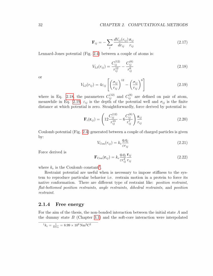
Lennard-Jones potential (Fig. 2.4) between a couple of atoms is:
VLJ(rij) =C
(12)ij
r12ij
−C
(6)ij
r6ij
(2.18)
or
VLJ(rij) = 4εij
[(σijrij
)12
−(σijrij
)6]
(2.19)
where in Eq. 2.18, the parameters C(12)ij and C
(6)ij are defined on pair of atom,
meanwhile in Eq. 2.19, εij is the depth of the potential well and σij is the finitedistance at which potential is zero. Straightforwardly, force derived by potential is:
Fi(rij) =
(12C
(12)ij
r13ij
− 6C
(6)ij
r7ij
)rijrij
(2.20)
Coulomb potential (Fig. 2.4) generated between a couple of charged particles is givenby:
VCou(rij) = keqiqjεrij
(2.21)
Force derived isFCou(rij) = ke
qiqjεr2ij
rijrij
(2.22)
where ke is the Coulomb constant1.Restraint potential are useful when is necessary to impose stiffness to the sys-
tem to reproduce particular behavior i.e. restrain motion in a protein to force itsnative conformation. There are different type of restraint like: position restraint,flat-bottomed position restraints, angle restraints, dihedral restraints, and positionrestraint.
2.1.4 Free energy
For the aim of the thesis, the non-bonded interaction between the initial state A andthe dummy state B (Chapter 3.1) and the soft-core interaction were interpolated
1ke = 14πε0
= 8.99× 10⁹ Nm2C2

2.1. MOLECULAR DYNAMICS 33
Figure 2.4: Non bonded interaction. On the left, the Lennard-Jones potential; onthe right Coulomb potential.
using a soft-core interaction. Consequently, bonded and non-bonded potential needto be restated taking the λ parameter in to account. The harmonic potential, theangle potential, and the improper dihedral angle are calculated in the spirit of thebond potential:
Vb =1
2
[(1− λ)kAb + λkBb
] [b− (1− λ)kA0 + λkB0
](2.23)
while for proper dihedral the equation is
Vd =[(1− λ)kAd + λkBd
] {1 + cos
[nφφ− (1− λ)φAs + λφBs
]}(2.24)
In this thesis work, the non bonded interaction, as Coulomb and Lennard-Jones,between molecules and solvent box has been subjected on a free energy routine. TheCoulomb and Lennard-Jones interactions variate on λ dependence as:
VC =1
εrfrij
[(1− λ) qAi q
Aj + λqBi q
Bj
](2.25)
VLJ =(1− λ)CB
12 + λCB12
rij12− (1− λ)CB
6 + λCB6
r6ij
(2.26)
Soft-core interaction and non-bonded interaction
The linear interpolation between of the non-bonded interaction as Lennard-Jones orCoulomb potentials weakly converge when particle are approaching to disappear asin dummy-particles formation. When λ value is near the limit to be zero or one

34 CHAPTER 2. COMPUTATIONAL METHODS
the interaction energy can be so feeble to permit particles collapse one against theother. The soft-core potentials remove this kind of undesirable singularities in thepotential. The specific non bonded interaction function between two atoms i and jis:
Vij(r) = (1− λ)V Aij (rAij)− λV B
ij (rBij) (2.27)
where
V Aij (rAij) =
(C
(12)ij
(rAij)12−
C(6)ij
(rAij)6
)+ ke
qiqjrAij
(2.28)
V Bij (rBij) =
(C
(12)ij
(rBij)12−
C(6)ij
(rBij)6
)+ ke
qiqjrBij
(2.29)
rAij = (α(σAij)6λp + r6
ij)1/6 (2.30)
rAij = (α(σBij )6(1− λ)p + r6
ij)1/6 (2.31)
where V Aij (rAij) and V B
ij (rBij) are the potential define the non-bonded interaction be-tween atoms i and j separated by a distance rij relative to the state A or the stateB. Van der Waals parameters for repulsions and the dispersion energy terms are,respectively, C
(12)ij and C
(6)ij ,k is equal to 1/(4πε0) and qi and qj are the atom charges.
The soft-core interaction parameters are the soft-core parameter p, the soft-core λpower p, and the radius of the interaction σ, which is (C(12)/C(6))1/6 or an inputparameter when C(6) or C(12) is zero
2.1.5 General simulation routine
MD simulation can be divided in several steps as reported in Fig. 2.5.
Initial condition To actuate the simulation, algorithm needs the topology infor-mation, as which atoms and which combination of atoms are participating,and a description of the force field. The box size, coordinates and velocities arenecessary. The box shape is defined by three vectors b1, b2, and b3. For ini-tiate the run the coordinates and t = t0 must be known. Dedicated algorithmupdate the time step by ∆t, also needs velocities at t = t0 − 1
2∆t. If velocities
are unknown, those are generated with a given absolute temperature T :
p(vi) =
√mi
2πkBTexp
(miv
2i
2kBT
)(2.32)
The total energy will be different to the required temperature T , this step needto be recalculated removing the motion of the center-of-mass and rescaling allvelocities so that the total energy correspond exactly to T .

2.1. MOLECULAR DYNAMICS 35
Figure 2.5: General scheme of a molecular dynamics simulation.
Neighbor searching Internal forces are defined by a tabulated list or from dynamiclists given by the non-bonded interaction between any pair of particles. Thenon-bonded pair interaction is calculated only if those pairs i, j is less than agiven cut-off radius Rc The pair list include particles i, a displacement vectorfor i and j. This list is updated every n steps.
Energy minimization Potential energy of N -interacting particle can be mappedin a so called potential energy surface or hypersurface. In geometrical way theenergy landscape is a representation of energy function across the configura-tion space of the system. In a system with N particles, energy is a function of(3N − 6) internal or 3N cartesian coordinates. Energy landscape has a globalminimum, that correspond to the stable system, and a collection of local min-ima. To identify the configuration with minimum energy that correspond tothe points in the configuration space is necessary use a minimization algorithm.Energy minimization process allow to find the nearest local minimum exploringthe energy landscape. Minima are located using numerical methods changingthe system coordinate gradually in the way to iteratively restart from a con-

36 CHAPTER 2. COMPUTATIONAL METHODS
figuration with lower energy. Hence, from a starting configuration the nearestminima is that one can be achieve methodically by the steepest local gradient.The minimization problem can be stated as find a minimum value of a func-tion f of a function which depends on more than one independent variables asx1, x2, . . . , xN . This topological places is defined when the first derivative ofthe function respect of all the variables is zero and the second derivatives areall positives:
∂f
∂xi= 0;
∂2f
∂x2i
> 0 wherei = ±1, 2, . . . , N (2.33)
With the second derivatives we can define a square N×N matrix called Hessianmatrix. This matrix has non-negative eigenvalues at the local minima. Betweenlocal minima can be defined the saddle point where eigenvalue is zero andthrough this points system can migrate from one local minimum to another.Energy minimization using different algorithm find the minima in the energylandscape like steepest descent, conjugate gradients, or l-bfgs.
The steepest descent algorithm is a first-order minimization method that slowlychange the coordinates of the atoms in the system in the aim to find a minima.Steepest descent move in the direction parallel to the net force calculated inthe previously. This algorithm needs a initial displacement h0 to start. Usinga geographical analogy the steepest descent move in downhill direction. Thevector r is defined by 3N coordinates. First forces F and potential energy arecalculated.
rn+1 = rn +Fn
|max(Fn)|hn (2.34)
where hn is the maximum displacement and Fn is the force calculated by thenegative gradient of the potential V . The value |max(Fn)| is the maximum ofthe absolute module of the force. The algorithm or when the maximum of theabsolute value of the force is smaller than a specified value.
Periodic Boundary conditions MD simulation system space are usually definedin boxes with different shape and dimension. In the way to decrease the artifactgenerated by this finite box system, periodic boundary condition are applied.MD compute the interaction with particle taking in to account copy of itselftranslated in a space-filling box.
Heating The heating steps impose a temperature at the system as in real experi-ment is done using a thermostatted heat bath. In this condition, the probability

2.1. MOLECULAR DYNAMICS 37
to find the system in a defined energy is given by the Boltzmann distribution:
f(p) =
(m
2πkBT
)3/2
exp
[−β p
2
2m
](2.35)
in molecular dynamics temperature is generally calculate using the relationbetween the temperature T and the and the kinetic energy per particle:
3
2kBT =
1
2m⟨v2j
⟩(2.36)
where m is the mass vj is the j-th component of the velocity. This calculationgive the temperature per particle in the system. This value is not the the systemtemperature, as the constant temperature in the system is not equivalent to thethe kinetic energy per particle. The variance of the kinetic energy per systemin the system can be cancel out if the kinetic energy for particle is defined equalto the average value of kinetic energy. The kinetic energy variance is given by:
σ2TK
〈TK〉2NV T=〈T 2
K〉NV T − 〈TK〉2NV T
〈p2〉2NV T=
2
3N(2.37)
Constant temperature ensemble needs a thermostats algorithm designed to helpthe simulation by modulating the temperature of the system in some desiredtemperature. Thermostat does not keep the temperature constant in time but,instead, ensure that the average temperature of a system is correct. Samplingin some small region in the system the kinetic energy of this small numberof particles fluctuate. Increasing the sample in a larger and larger number ofparticles, the fluctuations in the average get smaller and smaller, so for thewhole system constant temperature. So the role of a thermostat as ensuringthat we have the correct average temperature, and fluctuations of the correctsize.
Equilibration The constant pressure (NPT) procedure regulates the system a pres-sure. The gain in kinetic energy defined in the heating step generate a pressurethat can not be aligned with the prefixed experimental condition. In the samespirit of the thermostat algorithm a pressure coupling force the system to becoupled in a pressure bath. This type of algorithms rescale the box vector sizein the aim of reduce the pressure fluctuation around a defined average pressure.
Production run In this step the equilibrated system is monitored for defined timeof simulation. In this steps information about the trajectories and systemproperty are analyzed.
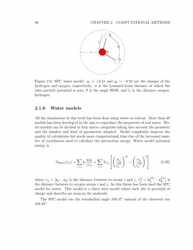
38 CHAPTER 2. COMPUTATIONAL METHODS
Figure 2.6: SPC water model. q1 = +0.41 and q2 = −0.82 are the charges of thehydrogen and oxygen, respectively. σ is the Lennard-Jones distance at which theinter-particle potential is zero, θ is the angle HOH, and l1 is the distance oxygen-hydrogen.
2.1.6 Water models
All the simulations in this work has been done using water as solvent. More than 40models has been developed in the aim to reproduce the properties of real water. Wa-ter models can be divided in four macro categories taking into account the geometryand the number and kind of parameters adopted. Model complexity improve thequality of calculation but needs more computational time due of the increased num-ber of coordinates used to calculate the interaction energy. Water model potentialenergy is
VWater(rij) =∑i<j
keqiqjεrij
+∑i<j
4εij
( σij
r(O)ij
)12
−
(σij
r(O)ij
)6 (2.38)
where rij = |rj − rk| is the distance between to atoms i and j, rOij = |r(O)
j − r(O)k | is
the distance between to oxygen atoms i and j. In this thesis has been used the SPCmodel for water. This model is a three sites model where each site is provided ofcharge and describe an atom in the molecule.
The SPC model use the tetrahedral angle 109.47◦ instead of the observed one104.32◦.
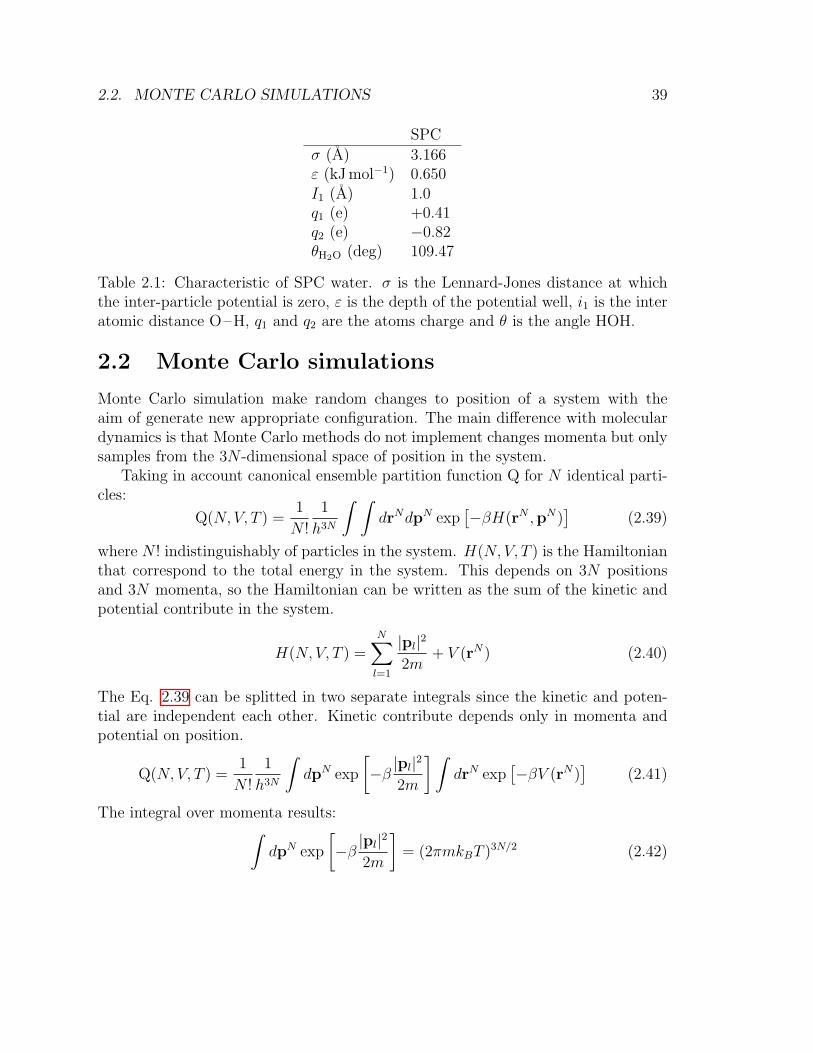
2.2. MONTE CARLO SIMULATIONS 39
SPC
σ (A) 3.166ε (kJ mol−1) 0.650I1 (A) 1.0q1 (e) +0.41q2 (e) −0.82θH2O (deg) 109.47
Table 2.1: Characteristic of SPC water. σ is the Lennard-Jones distance at whichthe inter-particle potential is zero, ε is the depth of the potential well, i1 is the interatomic distance O–H, q1 and q2 are the atoms charge and θ is the angle HOH.
2.2 Monte Carlo simulations
Monte Carlo simulation make random changes to position of a system with theaim of generate new appropriate configuration. The main difference with moleculardynamics is that Monte Carlo methods do not implement changes momenta but onlysamples from the 3N -dimensional space of position in the system.
Taking in account canonical ensemble partition function Q for N identical parti-cles:
Q(N, V, T ) =1
N !
1
h3N
∫ ∫drNdpN exp
[−βH(rN ,pN)
](2.39)
where N ! indistinguishably of particles in the system. H(N, V, T ) is the Hamiltonianthat correspond to the total energy in the system. This depends on 3N positionsand 3N momenta, so the Hamiltonian can be written as the sum of the kinetic andpotential contribute in the system.
H(N, V, T ) =N∑l=1
|pl|2
2m+ V (rN) (2.40)
The Eq. 2.39 can be splitted in two separate integrals since the kinetic and poten-tial are independent each other. Kinetic contribute depends only in momenta andpotential on position.
Q(N, V, T ) =1
N !
1
h3N
∫dpN exp
[−β |pl|
2
2m
] ∫drN exp
[−βV (rN)
](2.41)
The integral over momenta results:∫dpN exp
[−β |pl|
2
2m
]= (2πmkBT )3N/2 (2.42)
40 CHAPTER 2. COMPUTATIONAL METHODS
The integral over positions denoted as configuration integral Z(N, V, T ) results :
Z(N, V, T ) =
∫drN exp
[−βV (rN)
](2.43)
For non interacting particles potential energy function is zero. The exponential,straightforwardly, equal to 1 taking the the integral of 1 over the coordinate of eachatoms is the volume of the system for N non interacting particles. This result as:
Q(N, V, T ) =V N
N !
(2πkBTm
h2
)3N/2
(2.44)
This can also written in terms of the Broglie thermal wavelength Λ 2:
Q(N, V, T ) =V N
N !Λ3N(2.45)
From the Eq. 2.42 and 2.43 arise that the the partition function can be splitted intwo contributes: the momenta contribute, due by the gas behavior, and a contributegenerated by the interaction. The partition function for a system is settle up with acontribution due to momenta and a contribution between particles. All the deviationfrom an ideal gas are derived to the existence of interaction between the atoms inthe system. This energy is correlated only with position and not with momentaand Monte Carlo method is able to calculate the interaction contribution. Randommethod of sampling can be a possible alternative. To determinate the area underfunction curve we need to fix bounding area in which operate sampling. The ratio ofthe number of points under the curve to the total number of points, multiplied thesampling area estimate the area under the curve.
For potential energy is not possible solve analytically integral commonly usedin molecular modeling. In this limit case we need to find another path to evaluatethe integrals using numerical methods like the trapezium rule or the Simpson’s rule.Functions of two variables (x, y), for an accurate approximation need to square thenumber functions evaluations, so for a 3N -dimensional integral the total number orevaluations will be in the order of j3N where j is the particles number in a directions.For a 100 particles and 2 points for dimension we obtain 2200 evaluations!
2.3 Metropolis Method
In 1953 Metropolis et al. proposed a strategy to generate configuration that makea relevant contribution to the integral (Eq. 2.43). The Metropolis algorithm is a
2Λ =√h2/2πkBT

2.3. METROPOLIS METHOD 41
Markov chain Monte Carlo (MCMC) for obtaining a sequence of random samples.A Markov chain is stochastic model characterized by a finite set of events in whichthe probability of each event depends only on to the preceding one. This conditiondesignate a difference with the molecular dynamics method in which all states areconnected in time. This process is able to random generate a set of configuration witha probability proportional to the Boltzmann factor in a given temperature. Metropo-lis method routine change the phase space, from the configuration j in the systemmaking some predefined moves and test the new configuration j + 1. Test resultaccept the generated configuration j+ 1 if the energy is lower than the configurationj, otherwise if the the energy increases, it accepted only with probability:
p(∆E) = exp
[− ∆E
kBT ∗
](2.46)
where ∆E is the energetic gain respect of the configuration j and T ∗ is a fictitioustemperature.
Monte Carlo algorithm can be applicate to perform simulation of flexible molecules.The idea is based in applying random changes in the Cartesian coordinates of theatoms forming the molecule. This new configuration can be accepted by a accep-tance ratio defined a priori. The simplest model use a lattice approximation wherethe molecule is represented by the interaction of connected center. This center areenforced to be in the vertices of lattice. A more complex model are the beads modelwhere polymer is composed by subsequent sphere beads with defined radius beadand connection distance between consecutive object. Beads represent an effectivemonomer and interact with the first neighbor beads and with the nearby one. Thenew configuration is generated using a variant of the algorithm. This algorithm usea combination of crankshaft, reptation, and pivot end rotation move.
Crankshaft move select two random beads i,j where i < j, and with the conditionthat j − i ≤ k+ 2 where k � N . The number k represent the number of beads thatwill be rotate as the i+ 1, . . . j− 1 of an angle φ respect of the xi-xj axes. The angleis randomly chose in an given interval. Crankshaft move is a local move since only asmall portion of chain is changed. Pivot move select a random bead j internal to thebeads chain (1 ≤ j ≤ N − 1). This selected point act as fulcrum keeping fixed thethe beads 1, . . . , j − 1 and moving the j + 1, . . . , N chain of a random, range chose,value.

42 CHAPTER 2. COMPUTATIONAL METHODS

Chapter 3
Solvation free energy of aminoacids side chains
As precedently reported, classic Kauzmann et al. work point out that the trans-fer free energy between water and organic phase is favorable for hydrophobic sidechain analogs. Translated into the so-called hydrophobic effects in protein foldingthat tends to bury hydrophobic side chain inside the protein shielded from water. Inparallel experimental studies as reported in Chapter 1 underling the an additionalinterest in the understanding the effect of a specific solvent in protein stability. Molec-ular dynamics is a powerful tool that can provide useful and detailed informationon both the hydrophobic effect and the effect of solvent on protein stability. On theother hand, solvation free energy is most conveniently tackled using thermodynamicintegration rather then brute force molecular dynamics. In thermodynamics integra-tion, the free energy change of a solute upon gradually turning on the presence of thesolvent, is monitored. In this work, we have performed such calculation for 18 aminoacids, ranging from the most hydrophobic to the charged ones, and compared withpreviously known results, both experimental ans numerical. This calculation couldbe repeated for different solvents and small peptides, and is related to the approx-imate method in Chapter 4. Thermodynamic free energy is the amount of energyavailable in a system that can be converted in thermodynamic work. This quantitiesare useful values to understand the system at equilibrium. As precedently described,protein folding, as binding between molecules, or diffusion through a membrane areregulated by this energy. Free energy profile are useful to intimate understand how abiological or chemical process take place and put in evidence the kinetic and dynamicproperty. This type of calculation combined with numerical simulation are used inseveral areas as pharmacology, biochemistry, biotechnology and so on.
43
44CHAPTER 3. SOLVATION FREE ENERGY OF AMINO ACIDS SIDE CHAINS
3.1 Free energy
For a closed system σ with energy E, volume V , and number of particles N , theentropy S is at the maximum value only when the system is at equilibrium. Conse-quently, this system is not able to exchange heat, volume, or particles with a reser-voir. Two different function of state can be defined applying either a thermostattedbath,fixing the temperature T , the volume V and the number of particle N so thatthe Helmholtz free energy F = E − TS is at minimum at equilibrium, or couple thepressure to fix the pressure, and number of particles to set at minimum the Gibbs freeenergy G = E+PV . Comparing two system σT1 and σT2 with different temperatureT1 and T2 defined coupling a thermostatted bath and calculating the Helmholtz freeenergy, know which system is more stable. In classical mechanics the Helmholtz freeenergy F is
F (N, V, T ) = −kBT lnQ = −KBT ln
(∫d3pd3r exp[−βH(p, q)]
ΛN !
)(3.1)
where the Helmholtz free energy F is related with the partition function Q. Thermalquantities cannot be calculated directly neither in real experiment nor in numericalcalculation. Experiment give as result the derivative of a free energy respect to thevolume V or temperature T : (
∂F
∂V
)NT
= −P (3.2)
and (∂ FT
∂ 1T
)V N
= E (3.3)
The resulting pressure P and energy E can be measured in numerical calculation.Free energy of a system in a defined temperature and density can be calculatedfinding the path in V-T plane that connect the unknown state to a know one. Thechange in F is calculated with thermodynamic integration, integrating the equations3.2 and 3.3. To do this we need to define a referring state. The idea is use anideal gas phase for which free energy state as the thermodynamic state are alwaysknown. Numerical simulation permit to avoid this step building a state of referencemodifying the parameter that define the model feature.
Generally speaking,another purpose of a free energy calculation is calculate rel-ative energy between two different system like a receptor and a receptor with thebinded molecule, the difference in free energy between these systems due by the dock-ing is the energy of association. The difference in free energy between two states is

3.1. FREE ENERGY 45
Figure 3.1: Thermodynamic cycle for the determination of solvation energy.
A and B is
∆FAB = FA − FB = − 1
βlnQB
QA
(3.4)
where A and B are different conformations of the same system. The solvation freeenergy ∆Fsolv can be defined as the work necessary to transfer a molecule from a gasphase to a solution. This value is computationally obtainable in a reasonable amountof time and with a reasonable accuracy. Situation aforementioned can be solved usinga thermodynamic cycle and the Kirkwood’s coupling parameter method [44].
In the thermodynamic cycle represented in Fig. 3.1 ∆F3 is the work needed toremove the solute-solvent and solute-intramolecular interaction. The core idea residesin gradually mutate all the atoms in a given compound into a dummy atom. Thedummy atom peculiarity is that has the non bonded interactions, as the Lennard-Jones, set to zero but bonded interaction were kept unaltered. ∆F1 represent theenergy required to remove all the internal non-bonded interaction of the compound invacuo. ∆F2 is the work necessary to transfer dummy from vacuo to the solvent phase.Difference between two states can be determinate using thermodynamic integrationwhere Hamiltonian H is function of a parameter λ. The Hamiltonian of the systemchanges gradually from HA to HB. The coupling parameter of H(p, q, λ) in orderthat λ = 0 describes system A and λ = 1 describes system B:
H(p, q; 0) = HA(p, q) (3.5)
H(p, q; 1) = HB(p, q). (3.6)

46CHAPTER 3. SOLVATION FREE ENERGY OF AMINO ACIDS SIDE CHAINS
As precedently stated the partition function Q(N, V, T ) cannot be evaluated butit is possible to evaluate the derivative with respect to λ as an ensemble average
∆F (0→ 1) =
∫ 1
0
dλ∂F (λ)
∂(λ)= −
∫ 1
0
dλkBT1
Q
∂Q
∂(λ)(3.7)
∂F
∂(λ)=
1
N !h3N
∫∫dp dq
(−β∂H
∂λ
)exp [−βH(p, q, λ)] (3.8)
∂F
∂λ=
∫∫dp dq (∂H/∂λ) exp [−βH(p, q, λ)]∫∫
dp dq exp [−βH(p, q, λ)]=
⟨∂H
∂λ
⟩N,V,T,λ
(3.9)
The difference in free energy between A and B can be found by integrating thederivative over λ:
FB(V, T )− FA(V, T ) =
∫ 1
0
dλ
⟨∂H
∂λ
⟩N,V,T,λ
(3.10)
The λ-dependence of the potential in bonded interaction is liner while non-bondedinteraction can be described with linear dependence or with softcore interaction.
3.2 Bennett’s acceptance ratio method
Bennet in 1976 proposed a methodology to calculate the validate the free energybetween two state A and B using Metropolis Monte Carlo simulation [45]. The sameapproach called Bennett’s acceptance ratio (BAR) can be applied in thermodynamicintegration [46].
∆G(BAR)l→m = kBT
(ln〈f(Hl −Hm + C)〉m〈f(Hm +Hl − C)〉l
)+ C (3.11)
where f(x) is the Fermi function
f(x) =1
1 + exp(
xkBT
) (3.12)
Hl and Hm are the Hamiltonian in the states l and m. The constant C is calculatedevery iteration to fulfill the equivalence:
〈f(Hl −Hm + C)〉m = 〈f(Hm +Hl − C)〉l (3.13)

3.3. EXPERIMENTAL DATA FOR THE AMINO ACIDS 47
The free energy difference can be calculated as follows:
∆G(BAR)m→l = −kBT ln
Nm
Nl
+ C (3.14)
and
∆G(BAR)AB =
n−1∑A=l
∆G(BAR)l+1,m (3.15)
where Nl and Nm are the the number of coordinates for the lambda parameter λland λm, respectively. The accuracy of this processes can be insured only if there is asufficient overlap between the energy integrals. This overlap can be monitored withthe overlap integral.
3.3 Experimental data for the amino acids
The affinity of a molecule for an aqueous environment can be calculated with a vaporpressure calculation experiment. Experimental free energies solutes can be determi-nate calculating the concentration on two phase systems: the vapor phase with apartial pressure P
(Vap)m of some solute molecule of type m and the aqueous solution
with a concentration of solute as ρ(Aq)m . When these two phase are in equilibrium
with respect to the transfer of molecules of type between the phases, the solvationfree energy is given by
∆GSolv = kBT ln
(P
(Vap)m
ρ(Aq)m kBT
)(3.16)
when to state are in equilibrium the equilibrium constant K is given by
K =[state
(m)k ]
[state(m)j ]
(3.17)
Using moles instead of the number of molecules, the kB needs to be replaced withR. In the same way the use of concentration ρ
(Aq)m produce an extra kBT and the
logarithm term.1 where the equilibrium constant K is related to the free energy ofsolvation as follows:
∆G = −RT ln(K) = −RT ln
(state
(m)k
state(m)j
)= RT ln
(state
(m)j
state(m)k
)(3.18)
1The conversion from pressure to density, from number of molecules to moles, using nV =
PRT ,needs the use of kB contrariwise the R .

48CHAPTER 3. SOLVATION FREE ENERGY OF AMINO ACIDS SIDE CHAINS
Figure 3.2: Amino acid side chain neutral analogs.
Measuring the aqueous concentration the vapor pressure can be deducted indirectly:
∆G = RT ln
([m(aq)]i − [m(aq)]f
[m(aq)]f
)= RT ln
([m(aq)]i[m(aq)]f
+ 1
)(3.19)
where [m(aq)]f and [m(aq)]i are the final concentration, at equilibrium, and initialconcentration, respectively.
3.4 Free energy calculation of single amino acid
The hydratation free energy has been calculated using thermodynamic integrationas described in chapter (3.1). For each molecule the free energy calculation has beenderived using n-different calculation as many λ points from λA = 0 (solute) to λB = 1(dummy atoms). Compound investigated are the neutral analog of the amino acidside chain (Fig. 3.2). Each analog correspond to the side chain starting from theβ-carbon. The truncated bond as been substituted with an hydrogen atom. Allthe compound investigated are in neutral form, so electrically charged amino acid asbeen neutralized adding or removing a proton.

3.5. RESULTS 49
3.4.1 Free energy calculation routine
The simulation were performed at constant temperature and pressure in cubic box.The force field used was gromos54a7 modified accordingly (from here onwards GRO-MOS(ATB)). This revised force field has been customized in bonded and non bondedinteraction using building blocks and interaction parameter from Automated Topol-ogy Builder (ATB) [47–50]. The neighbor searching distance was defined as Verletwith a searching distance of 1.2 nm. Solvation has been set to build a shell of 1 nmof SPC water around the molecule shaping a ≈3 nm box with ≈900 water molecules.The non bonded interaction were set as 1.2 nm for the electrostatic parameter,thevan der Waals set as Particle-Mesh Ewald (PME) and cutoff, respectively. Theisothermal-isobaric ensemble at 300 K,a leap-frog stochastic dynamics integrator (sd)has been used to integrate the equations of motion. Pressure has been maintainedconstant using the Parrinello-Rahman barostat. Pressure has been set as 1 atm.The inverse friction constant as been set as 1.0 ps Water compressibility was setas 4.5× 10⁻⁵ bar−1. Free energy parameters were evaluated starting with 0.05 in-crement in λ parameters (from 0.00 to 1.00) for a total of 20 λ. Thermodynamicintegration has been calculated transforming Coulomb ans Van der Waals interactionwith the same rate. Simulation was recalculated, increasing the value of λ steps, ifBennett Acceptance Ratio was not achieved. Decoupling parameter for soft-core α,σ and p parameter were set as 0.5, 0.3 and 1. The angles and the bond distanceswere constrained using LINCS algorithm with the highest order in the expansion ofthe constraint coupling matrix set as 12. Time steps in each simulation was 0.002 psand 50000 steps for a total of 100 ps for NVT and NPT routines. Production runhas been simulated with time steps of 0.002 ps and 500000 steps for a total of 1 ns
3.5 Results
Free energy calculation were performed from a fully interacting neutral analog toa non interacting molecule. Assuming the reversibility of the processes, so startingwith a complete uncoupled compound in water and gradually turn off the interaction,the energy value change in sign. This transformations required a minimum of 20 λpoints and a maximum of 34 λ. The calculated hydratation free energy statisticalerror is in the range 0.11 kJ mol−1 to 0.49 kJ mol−1. The process produced duringthe free energy calculation, compound interaction with solvent are gradually turnedoff until the dummy state. Simulation has been done at 300 K, on the other handsome experimental and calculated simulation has been done with different referencetemperature (Villa et al. (T = 293 K); Wolfenden et al. (T = (298.15 K)). Change
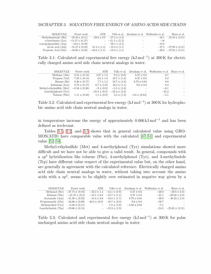
50CHAPTER 3. SOLVATION FREE ENERGY OF AMINO ACIDS SIDE CHAINS
MOLECULE Preset work ATB Villa et al. Abraham et al. Wolfenden et al. Rizzo et al.Methylimidazole (His) −28.48± (0.11) −29.6± 0.9 −27.4± (1.2) - −42.1 −35.19± (2.51)
n-butylamine (Lys) −13, 27± (0, 27) - −15, 5± (2, 2) - −18 -n-propylguanidine (Arg) −44.6± (0.49) - −30.1± (2.4) - −44.8 -
Acetic acid (Asp) −31.27± (0.33) 31.4± (1.4) −18.2± (1.1) - −27.5 −27.99± (2.51)Propionic Acid (Glu) −34.66± (0.33) −34.8± (1.5) −16.2± (1.1) - −26.6 −27.03± (2.51)
Table 3.1: Calculated and experimental free energy (kJ mol−1) at 300 K for electri-cally charged amino acid side chain neutral analogs in water.
MOLECULE Preset work ATB Villa et al. Abraham et al. Wolfenden et al. Rizzo et al.Methane (Ala) 8.54± (0.12) 4.27± 1.0 9.2± (0.6) 6.27± 0.6 8.1 -Propane (Val) 7.93± (0.14) 6.6± 1.0 10.7± (1.2) 8.37± 0.8 8.2 -
Butane (Ile) 8.36± (0.17) 7.7± 1.2 10.7± (1.0) 8.79± 0.84 8.8 -Isobutane (Leu) 8.72± (0.17) 6.7± (1.0) 10.4± (1.1) 9.6± 0.8 9.4 -
Methyl-ethylsulfide (Met) −0.58± (0.28) −9± (0.9) −5.5± (1.0) - −6.1 -4-methylphenol (Tyr) - −25.5± (0.5) −22.4± (2.2) - −25.2 -
Toluene (Phe) 1.11± (0.23) 1.1± (0.8) 3.4± (1.3) −3.8± (0.84) −3.1 -
Table 3.2: Calculated and experimental free energy (kJ mol−1) at 300 K for hydropho-bic amino acid side chain neutral analogs in water.
in temperature increase the energy of approximately 0.006 kJ mol−1 and has beendefined as irrelevant.
Tables 3.1, 3.2, and 3.5 shows that in general calculated value using GRO-MOS(ATB) have comparable value with the calculated [47, 51] and experimentalvalue [52–54].
Methyl-ethylsulfide (Met) and 4-methylphenol (Tyr) simulations showed moredifficult and we have not be able to give a valid result. In general, compounds witha sp2 hybridization like toluene (Phe), 4-methylphenol (Tyr), and 3-methylindole(Trp) have different value respect of the experimental value but, on the other hand,are generally in agreement with the calculated reference. Electrically charged aminoacid side chain neutral analogs in water, without taking into account the aminoacids with a sp2, seems to be slightly over estimated in negative way given by a
MOLECULE Preset work ATB Villa et al. Abraham et al. Wolfenden et al. Rizzo et al.Methanol (Ser) −27.75± (0.19) −22.2± 1.4 −14.1± (0.9) 6.27± 0.6 −20.8 −20.8± 2.51Ethanol (Thr) −21.37± (0.2) −19.1± 0.8 −13.7± (1.1) 8.37± 0.8 −21.1 −20.92± 2.51
Acetamide (Asn) −41.38± (0.33) −41.8± 0.6 −18.8± (1.7) 8.79± 0.84 −39.9 −40.23± 2.51Propionamide (Gln) −44.66± (0.09) −40.3± (0.9) −18.7± (2.0) 9.6± 0.8 −38.7 -Methanethiol (Cys) −8.38± (0.11) - 5.5± (1.0) −5.02± 0.84 −5.1 -
3-methylindole (Trp) −19.66± (0.14) - −12.3± (1.9) - −24.3 −25.65± (2.51)
Table 3.3: Calculated and experimental free energy (kJ mol−1) at 300 K for polaruncharged amino acid side chain neutral analogs in water.
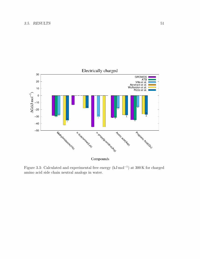
3.5. RESULTS 51
Figure 3.3: Calculated and experimental free energy (kJ mol−1) at 300 K for chargedamino acid side chain neutral analogs in water.

52CHAPTER 3. SOLVATION FREE ENERGY OF AMINO ACIDS SIDE CHAINS
Figure 3.4: Calculated and experimental free energy (kJ mol−1) at 300 K for hy-drophobic charged amino acid side chain neutral analogs in water.

3.5. RESULTS 53
Figure 3.5: Calculated and experimental free energy (kJ mol−1) at 300 K for polaruncharged amino acid side chain neutral analogs in water.
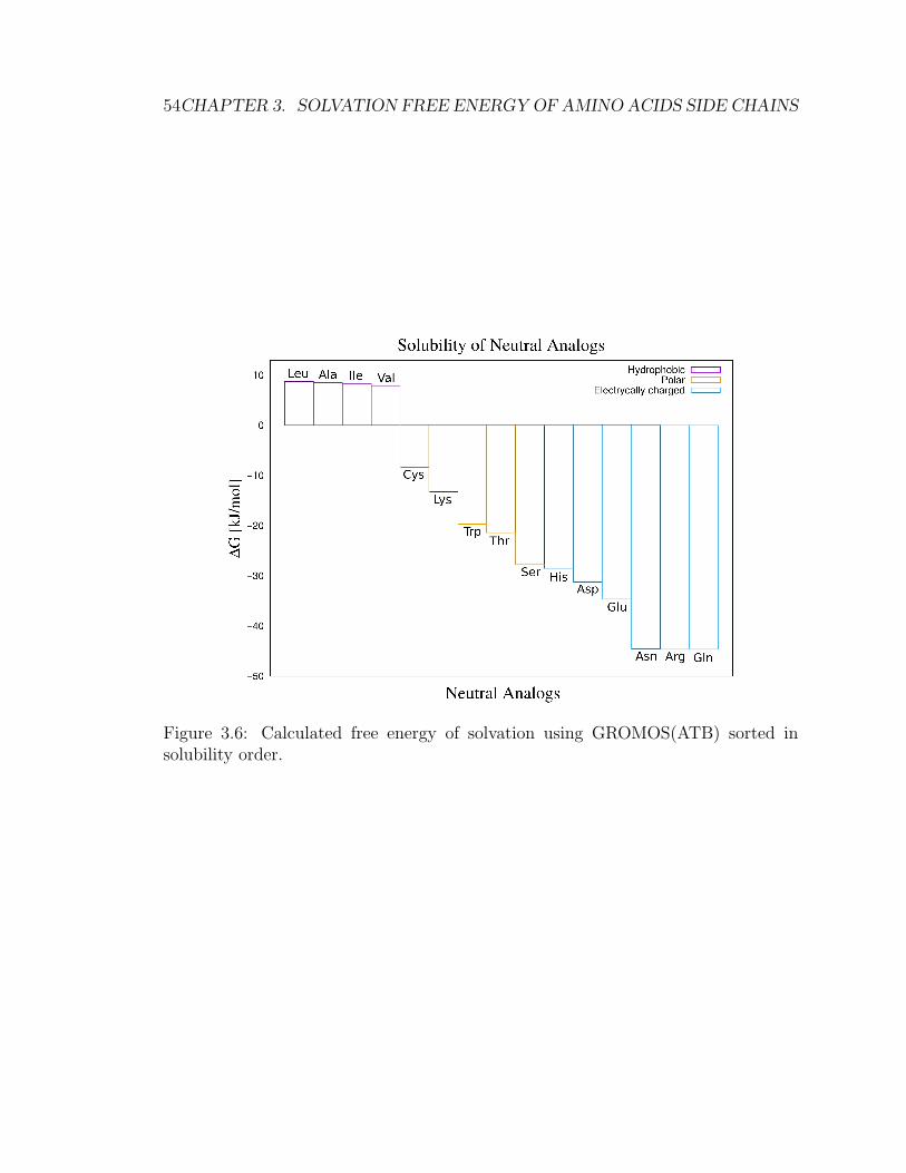
54CHAPTER 3. SOLVATION FREE ENERGY OF AMINO ACIDS SIDE CHAINS
Figure 3.6: Calculated free energy of solvation using GROMOS(ATB) sorted insolubility order.

3.5. RESULTS 55
force field distortion that induces the analogs to by more hydrophilic then expected.In contrast, polar uncharged amino acids, are in good agreement with the experi-mental value. Methyl-ethylsulfide (Met), as methanethiol (Cys), show an anomalousbehavior probably due to the tioeter group R–S–R.
Figs. from 3.8 to 3.10 show the cumulative ∆G as function of λ. The value ofcumulative value in ∆G is obtained by the sum of two consecutive λ value. If, forinstance, λ = 0 is 0.3 kJ mol−1 and in λ = 0.02 is 0.5 kJ mol−1 the cumulative value is0.8 kJ mol−1. Formally,it is the integral of all the ∆G during the uncoupling process:∫ λ
0
(dG
dλ′
)dλ′ (3.20)
Bennet acceptance ratio algorithm generate useful information to understand theinteraction during the decoupling. From Fig. 3.8 toluene (Phe) and 3-methylindole(Trp) share the same pattern as highlighted in Fig. 3.7. These structures share a six-membered benzene ring, but tryptophan analog λ = 0 is negative (−3.12 kJ mol−1).This affinity could be generated by the secondary amine in the pyrrolic ring able toform a H-bond with water. Decoupling process change this value in one step leadingthe 3-methylindole (Trp) to ensue the patter of a the hydrophobic Toluene (Phe).
(a) (b)
Figure 3.7: (a) dG/dλ for toluene (Phe) with λ = 20; (b) dG/dλ for 3-methylindole(Thr) with λ = 24. This compounds have, qualitatively, the similar decouplingprocess.
Methane (Ala), propane (Val), butane (Ile), isobutane (Leu), and methyl-ethylsulfide(Met) in Fig. 3.8 share same cumulative ∆G pattern as in the ∆G function of λ value(Figs. 3.11(a) to 3.11(e)). These compounds are generally hydrophobic and not so

56CHAPTER 3. SOLVATION FREE ENERGY OF AMINO ACIDS SIDE CHAINS
Figure 3.8:∫ λ
0
(dGdλ′
)dλ′ for the Hydrophobic analogs: methane (Ala), propane
(Val), isoleucine (Ile), isobutane (Leu), methyl-ethylsulfide (Met), toluene (Phe),and 4-methylphenol (Trp).
Figure 3.9:∫ λ
0
(dGdλ′
)dλ′ for the Polar uncharged analogs: methanol (Ser), ethanol
(Thr), acetamide (Asn), propionamide (Gln), and methanethiol (Cys).

3.5. RESULTS 57
Figure 3.10:∫ λ
0
(dGdλ′
)dλ′ for the Electrically charged analogs: methylimidazole
(His), n-butylamine (Lys), n-propylguanidine (Arg), acetic acid (Asp), and propioncacid (Glu).
well solubilized in water. Methyl-ethylsulfide, as Wolfenden et al. report, slightlysoluble in water (∆G =−6.1 kJ mol−1). This value is different from the calculatedone ∆G =−0.58 kJ mol−1, but the similar pattern could suggest that this arise froman overstatement of the tioeter group R–S–R by the force field.
Polar amino acid neutral compounds cumulative solvation free energies are re-ported in Fig. 3.9. Acetamide (Asn) and propionamide (Gln) have similar patternas in the Figs. 3.12(a) and 3.12(b) These molecules are miscible in water and asfor the 3-methylindol (Trp) the first λ abruptly change the interaction with water.Methanethiol (Cys) profile in Fig 3.9 is vaguely related with acetamide and propi-onamide one. The cumulative free energy (Fig. 3.12(c)) is characterized with twodrops (7/34λ value ∆λ = 0.206 and 20/34λ value ∆λ = 0.588). Even in this case,as precedently supposed, the thiol group –SH an overstate free energy of solvation.
Methanol (Ser) and Ethanol (Thr) in Figs. 3.13(a) and 3.13(b) share a peculiardrop in at one-third of the decoupling (methanol: 7/20λ value, λ = 0.35; Ethanol:8/24λ value, λ = 0.33). These compound are characterized by an hydroxyl group–OH and the drop can be associated with this feature.
From Fig. 3.10 methylimidazole (His), acetic acid (Asp), and propionic acid(Glu) can be correlated in one trend, as n-butylamine (Lys), n-propylguanidine
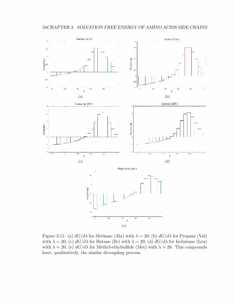
58CHAPTER 3. SOLVATION FREE ENERGY OF AMINO ACIDS SIDE CHAINS
(a) (b)
(c) (d)
(e)
Figure 3.11: (a) dG/dλ for Methane (Ala) with λ = 20; (b) dG/dλ for Propane (Val)with λ = 20; (c) dG/dλ for Butane (Ile) with λ = 20; (d) dG/dλ for Isobutane (Leu)with λ = 20; (e) dG/dλ for Methyl-ethylsulfide (Met) with λ = 20. This compoundshave, qualitatively, the similar decoupling process.

3.5. RESULTS 59
(a) (b)
(c)
Figure 3.12: (a) dG/dλ for acetamide (Asn) with λ = 20; (b) dG/dλ for propi-onamide (Gln) with λ = 32; (c) (b) dG/dλ for methanethiol (Cys) with λ = 3. Thiscompounds have, qualitatively, the similar decoupling process.

60CHAPTER 3. SOLVATION FREE ENERGY OF AMINO ACIDS SIDE CHAINS
(a) (b)
Figure 3.13: (a) dG/dλ for methanol(Ser) with λ = 23; (b) dG/dλ for ethanol(Thr)with λ = 24. This compounds have, qualitatively, the similar decoupling process.
(Arg), acetic acid (Asn), and propionic acid (Gln) in a second one. Acetic acidand propionic acid (Figs. 3.14(a) and 3.14(b)) patterns look more alike than themethylimidazole one (Fig. 3.14(c)) since these have a positive ∆G as function ofλ in the final part, controversially, methylimidazole ∆G as function of λ is nega-tive. Furthermore, acetic acid and propionic acid are correlated by the presence ofa carboxylic group –COOH. The n-butylamine, n-propylguanidine, acetic acid, andpropionic acid group is characterized by side chain with an amidic group in the sidechain. Moreover, n-butylamine and n-propylguanidine, characterized by a primaryamine group –NH2 and guanidino group –HN–C–N2H3 respectively, have similarpattern (Figs. 3.15(a) and 3.15(b)) therefore, asparagine (Asn) and glutamine (Gln)due the presence of the amide group –CONH2.

3.5. RESULTS 61
(a) (b)
(c)
Figure 3.14: (a) dG/dλ for acetic acid (Asp) with ∆λ = 20; (b) dG/dλ for propionicAcid (Glu) with ∆λ = 20; (c) dG/dλ for methylimidazole (His) with ∆λ = 20 Thiscompounds have, qualitatively, the similar decoupling process.

62CHAPTER 3. SOLVATION FREE ENERGY OF AMINO ACIDS SIDE CHAINS
(a) (b)
Figure 3.15: (a) dG/dλ for n-butylamine (Lys) with λ = 20; (b) dG/dλ for n-propylguanidine (Arg) with λ = 20. This compounds have, qualitatively, the similardecoupling process.
Chapter 4
Protein folding in non watersolvent
In Chapter 3 we discussed how to compute the solvation free energy of a solute inwater, as well as in other solvents, using thermodynamic integration. This calculationhas been used in the case of single amino acid side chains. Comparison with previous,both experimental and numerical works, showed consistent results, indicating thesoundness of this approach. Scaling up the system to the simulation of a full protein,however, proves a very challenging task. In this chapter we present an alternativeapproach, hinging upon an approximated method called morphometric approach,to evaluate the solvent free energy. This approach was devised by a group at theUniversity of Kyoto whom we have been collaborating with. In protein simulationa decoys is used generally to compare a native protein with alternative geometricalstructure in the way of test algorithm able to identify a native state [55]. Park andLevitt [56] used decoys conformations to investigate the ability of numerical methodsto distinguish, contact and surface area, and distance-dependent energy betweennative configuration and decoys set. Decoys are even used to generate large set ofconfiguration as prediction to ab initio methods, that require vast computationalresources, and select the most fitting ones based on a scoring or free energy function[57]. The several strategies able to generate protein decoys are correlated by thatstructures are slightly different from the native structure generally in orded of 5 A to20 A [57,69]. This feature is a direct consequence of the former application. Withinthe morphometric method, however, this thesis contributes to develop a bioinformatictool capable to build several alternative decoys with a huge variety of topology andprescribed secondary structure content. Structure like the just mentioned will be usedto calculate the difference in stability between the native state and the several decoys
63
64 CHAPTER 4. PROTEIN FOLDING IN NON WATER SOLVENT
generate both in water than in other solvents. Using as framework a precedent work,the general procedure to generate decoys has been kept, we looked for significantlyimprove the efficiency of structures generated and structures information useful forpopulation studies.
The protein folding process leads protein to a well defined three-dimensionalstructure called ”native structure” in physiological environment. The commonlyaccepted protein folding mechanism hinges upon the idea that all the informationrequired for a protein to reach the native conformation are encoded in its primarysequence. The native state is consequence of the complex interplay of physical fac-tors. Protein folding can be split in a three steps thermodynamic cycle: proteindesolvatation, the relaxation of the structure and the solvation of the completelyunfolded structure. Change in free energy by the folding process is defined as:
∆G(Folding) = ∆H(Folding) − T∆S(Folding) = −∆G(Unfolding) (4.1)
where ∆H e ∆S are the change in enthalpy and entropy in the system. The changein free energy can be calculated using thermodynamic integration as
∆G(Unfolding)(λ=0) = ∆G
(Native)(0→1) + ∆G
(Unfolded)(λ=1) −∆G
(Unfolded)(0→1) . (4.2)
where (λ = 0) is the total interaction of the protein with water and (λ = 1) describesthe system completely decoupled. ∆GNative
(0→1) are the ∆GUnfolded(0→1) change in free energy
due of the path done from the complete coupled state to the uncoupled one. UsingMD simulation as proved in Chapter 3 is able to calculate free energy of solvationfor a single amino acids. Proteins solvation free energy
Protein folding can be regarded as sum of different contributions. The hy-drophobic effect, decrease in protein intramolecular electrostatic interaction energy,decrease in protein intramolecular van der Waals interaction energy, the lose ofconformational-entropy of protein, and the increase in protein-water electrostaticinteraction energy.
The increase in protein-water electrostatic interaction energy entail a deceasein water-water electrostatic interaction energy. During protein folding process theamount of solvatable surface in the protein decrease forcing water molecules to re-organize the solvent configuration. The contrasting contribute of these outlinedprocesses sums implying a partial cancel-out of the energy increase in protein-waterelectrostatic interaction energy. Increase in protein-water Van der Waals interactionenergy leads a change in water-water van der Waals interaction energy as the waterreorganization.
The canonical concept of hydrophobic effect by the idea that a protein definean excluded volume which solvent cannot access. [58–61]. The same concept can

4.1. MODEL 65
by applied for the water molecules itself. Water occupy a volume that cannot beaccessed by the other water molecules in the solvent consequently molecules in thesolvent are etropically correlated create an effect defined as water crowding [59–61].Folding leads to an increase in volume accessible for the solvent molecules which aremore capable to move. This entropy gain, that is an immediate consequence to thereduction of water crowding, has been named as entropic excluded-volume.
For this studies has been choose two protein. First protein is a CREB protein(Fig. 4.1 (a)), the 4ouf [65] protein with a total structure weight of 28 050.16 Da, 238residues, homo 2-mero stoichiometry. This protein as focal role in the transcritpionalcoactivation of different transcription factors, regulating the growth control and theembryonic development. This family share the histone acetyltransferase activity bywhich catalyze the lysine amino acids on histone proteins. Histones are a proteinsthat package the DNA in nucleosome. The lysine acetylation permit the dissociationof histones from DNA promoting the gene expression. The chain A of this protein asbeen choose to depict the all-α protein category since this 114 residues protein have62% of helical structure (two 310 helices, four α-helices, 73/114 residues participants)as reported in Fig. 4.2(a).
The second proteins (Fig. 4.1 (b)), 2pcy [66] (10 493.61 Da, 99 residues and738 atoms), is an apoplastocynin protein, electron transport protein located in theapoplast, a continuum between two plant cell walls, that have as principal role thewater and solute transport. 2pcy has been choose as the all-β reference structurebecause of only the 6% of α-helices (two 310 helices, 6/99 residues participants) and40% β-sheet (ten strands, 40/99 residues participants) as reported in Fig. 4.2(b).
4.1 Model
This section explain which models has been take into account to explore the physicalproperty that permit the stability of a folded protein in a defined solvent. Two orderof effects has been selected: the water crowding based on the entropic excluded-volume concept, and the H-bonds acceptor-donor interaction. In a solvated proteincan occur three type hydrogen bonds: protein intramolecular (P-P), protein-water(P-W) and water-water (W-W) . The hydrophobic effect as entropic excluded-volumehinges on the physico-chemical characteristics of the solvent. With the idea of explorethe hierarchy of interaction in the protein-solvent system eight models have been builtup. Proteins are taken into account at atomistic level using neutral hard-spherecentered in the (x,y,z) coordinates of the atoms position with diameter set as thecorresponding value of Lennard-Jones parameter, σ to substitute the atom position.Models are defined by the combination of some common features: HS (hard spheres)
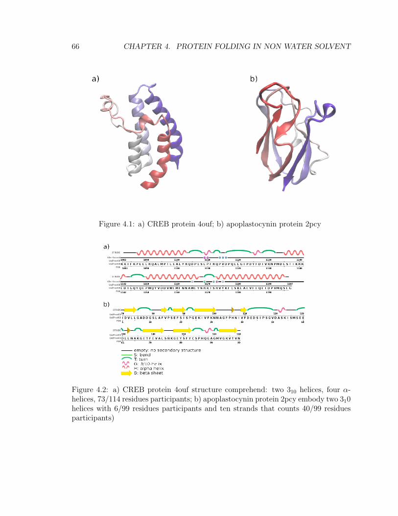
66 CHAPTER 4. PROTEIN FOLDING IN NON WATER SOLVENT
Figure 4.1: a) CREB protein 4ouf; b) apoplastocynin protein 2pcy
Figure 4.2: a) CREB protein 4ouf structure comprehend: two 310 helices, four α-helices, 73/114 residues participants; b) apoplastocynin protein 2pcy embody two 310helices with 6/99 residues participants and ten strands that counts 40/99 residuesparticipants)
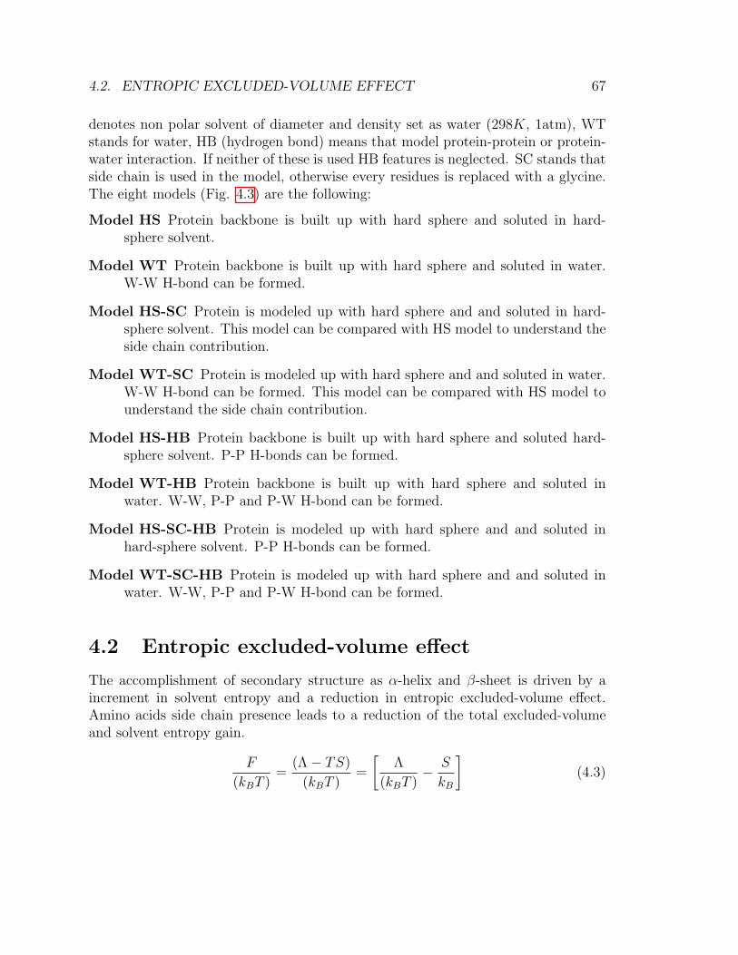
4.2. ENTROPIC EXCLUDED-VOLUME EFFECT 67
denotes non polar solvent of diameter and density set as water (298K, 1atm), WTstands for water, HB (hydrogen bond) means that model protein-protein or protein-water interaction. If neither of these is used HB features is neglected. SC stands thatside chain is used in the model, otherwise every residues is replaced with a glycine.The eight models (Fig. 4.3) are the following:
Model HS Protein backbone is built up with hard sphere and soluted in hard-sphere solvent.
Model WT Protein backbone is built up with hard sphere and soluted in water.W-W H-bond can be formed.
Model HS-SC Protein is modeled up with hard sphere and and soluted in hard-sphere solvent. This model can be compared with HS model to understand theside chain contribution.
Model WT-SC Protein is modeled up with hard sphere and and soluted in water.W-W H-bond can be formed. This model can be compared with HS model tounderstand the side chain contribution.
Model HS-HB Protein backbone is built up with hard sphere and soluted hard-sphere solvent. P-P H-bonds can be formed.
Model WT-HB Protein backbone is built up with hard sphere and soluted inwater. W-W, P-P and P-W H-bond can be formed.
Model HS-SC-HB Protein is modeled up with hard sphere and and soluted inhard-sphere solvent. P-P H-bonds can be formed.
Model WT-SC-HB Protein is modeled up with hard sphere and and soluted inwater. W-W, P-P and P-W H-bond can be formed.
4.2 Entropic excluded-volume effect
The accomplishment of secondary structure as α-helix and β-sheet is driven by aincrement in solvent entropy and a reduction in entropic excluded-volume effect.Amino acids side chain presence leads to a reduction of the total excluded-volumeand solvent entropy gain.
F
(kBT )=
(Λ− TS)
(kBT )=
[Λ
(kBT )− S
kB
](4.3)
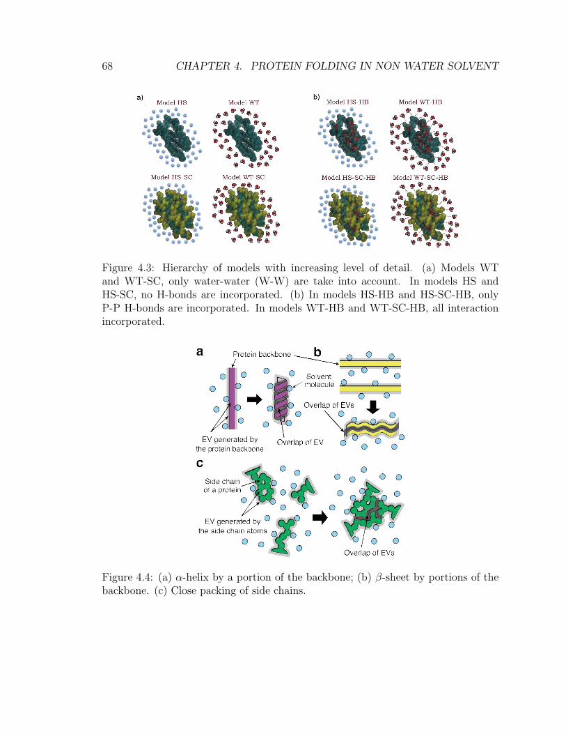
68 CHAPTER 4. PROTEIN FOLDING IN NON WATER SOLVENT
Figure 4.3: Hierarchy of models with increasing level of detail. (a) Models WTand WT-SC, only water-water (W-W) are take into account. In models HS andHS-SC, no H-bonds are incorporated. (b) In models HS-HB and HS-SC-HB, onlyP-P H-bonds are incorporated. In models WT-HB and WT-SC-HB, all interactionincorporated.
Figure 4.4: (a) α-helix by a portion of the backbone; (b) β-sheet by portions of thebackbone. (c) Close packing of side chains.
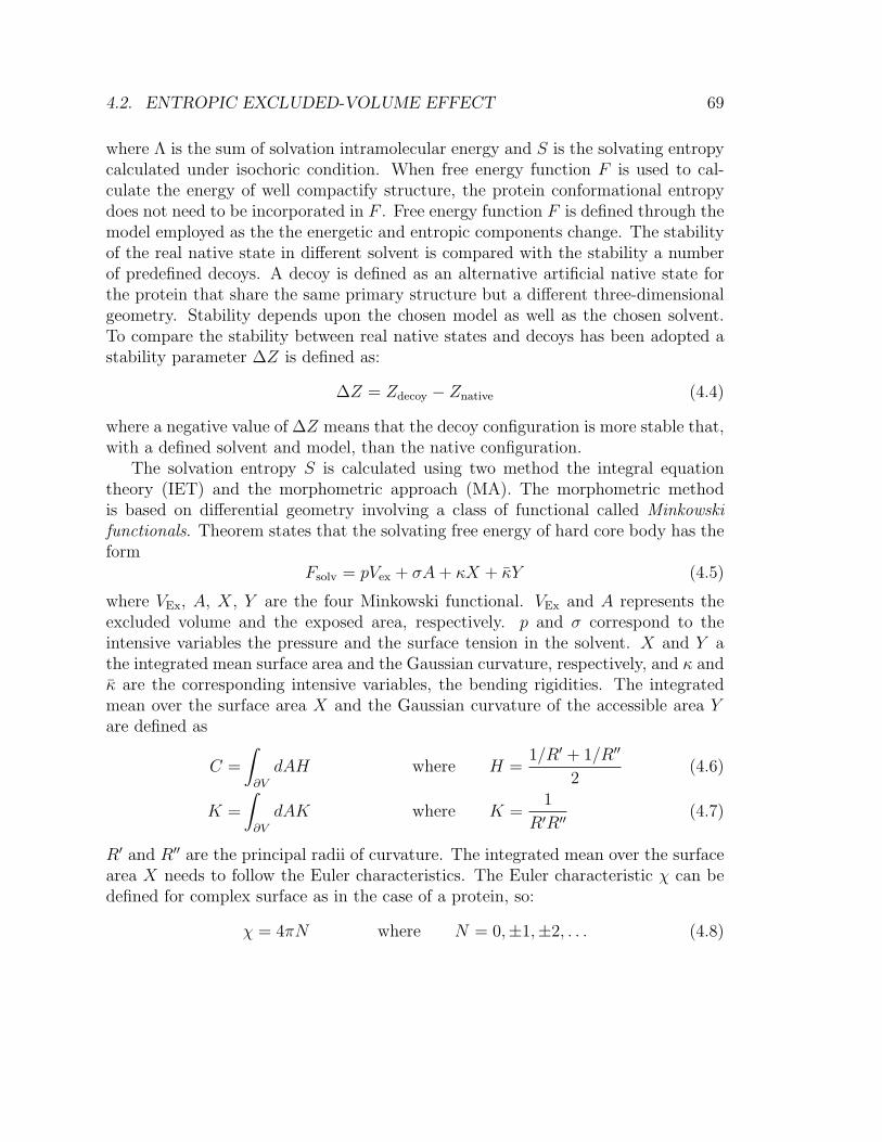
4.2. ENTROPIC EXCLUDED-VOLUME EFFECT 69
where Λ is the sum of solvation intramolecular energy and S is the solvating entropycalculated under isochoric condition. When free energy function F is used to cal-culate the energy of well compactify structure, the protein conformational entropydoes not need to be incorporated in F . Free energy function F is defined through themodel employed as the the energetic and entropic components change. The stabilityof the real native state in different solvent is compared with the stability a numberof predefined decoys. A decoy is defined as an alternative artificial native state forthe protein that share the same primary structure but a different three-dimensionalgeometry. Stability depends upon the chosen model as well as the chosen solvent.To compare the stability between real native states and decoys has been adopted astability parameter ∆Z is defined as:
∆Z = Zdecoy − Znative (4.4)
where a negative value of ∆Z means that the decoy configuration is more stable that,with a defined solvent and model, than the native configuration.
The solvation entropy S is calculated using two method the integral equationtheory (IET) and the morphometric approach (MA). The morphometric methodis based on differential geometry involving a class of functional called Minkowskifunctionals. Theorem states that the solvating free energy of hard core body has theform
Fsolv = pVex + σA+ κX + κY (4.5)
where VEx, A, X, Y are the four Minkowski functional. VEx and A represents theexcluded volume and the exposed area, respectively. p and σ correspond to theintensive variables the pressure and the surface tension in the solvent. X and Y athe integrated mean surface area and the Gaussian curvature, respectively, and κ andκ are the corresponding intensive variables, the bending rigidities. The integratedmean over the surface area X and the Gaussian curvature of the accessible area Yare defined as
C =
∫∂V
dAH where H =1/R′ + 1/R′′
2(4.6)
K =
∫∂V
dAK where K =1
R′R′′(4.7)
R′ and R′′ are the principal radii of curvature. The integrated mean over the surfacearea X needs to follow the Euler characteristics. The Euler characteristic χ can bedefined for complex surface as in the case of a protein, so:
χ = 4πN where N = 0,±1,±2, . . . (4.8)
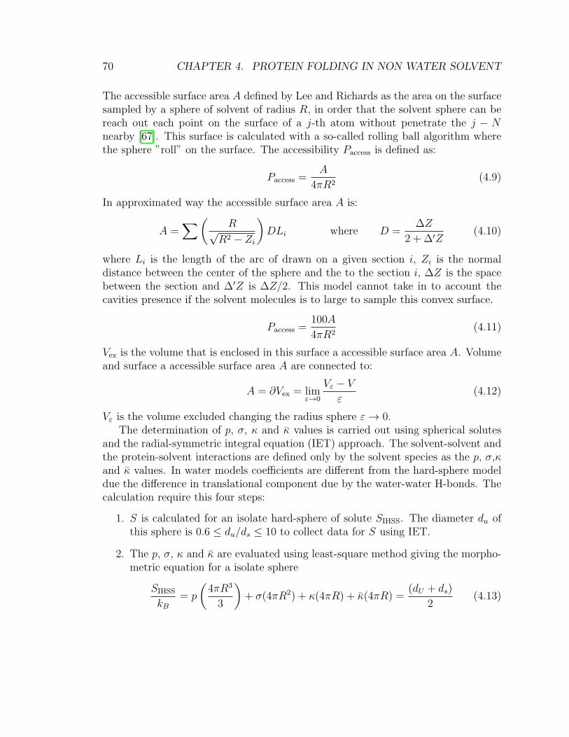
70 CHAPTER 4. PROTEIN FOLDING IN NON WATER SOLVENT
The accessible surface area A defined by Lee and Richards as the area on the surfacesampled by a sphere of solvent of radius R, in order that the solvent sphere can bereach out each point on the surface of a j-th atom without penetrate the j − Nnearby [67]. This surface is calculated with a so-called rolling ball algorithm wherethe sphere ”roll” on the surface. The accessibility Paccess is defined as:
Paccess =A
4πR2(4.9)
In approximated way the accessible surface area A is:
A =∑(
R√R2 − Zi
)DLi where D =
∆Z
2 + ∆′Z(4.10)
where Li is the length of the arc of drawn on a given section i, Zi is the normaldistance between the center of the sphere and the to the section i, ∆Z is the spacebetween the section and ∆′Z is ∆Z/2. This model cannot take in to account thecavities presence if the solvent molecules is to large to sample this convex surface.
Paccess =100A
4πR2(4.11)
Vex is the volume that is enclosed in this surface a accessible surface area A. Volumeand surface a accessible surface area A are connected to:
A = ∂Vex = limε→0
Vε − Vε
(4.12)
Vε is the volume excluded changing the radius sphere ε→ 0.The determination of p, σ, κ and κ values is carried out using spherical solutes
and the radial-symmetric integral equation (IET) approach. The solvent-solvent andthe protein-solvent interactions are defined only by the solvent species as the p, σ,κand κ values. In water models coefficients are different from the hard-sphere modeldue the difference in translational component due by the water-water H-bonds. Thecalculation require this four steps:
1. S is calculated for an isolate hard-sphere of solute SIHSS. The diameter du ofthis sphere is 0.6 ≤ du/ds ≤ 10 to collect data for S using IET.
2. The p, σ, κ and κ are evaluated using least-square method giving the morpho-metric equation for a isolate sphere
SIHSS
kB= p
(4πR3
3
)+ σ(4πR2) + κ(4πR) + κ(4πR) =
(dU + ds)
2(4.13)

4.3. THE ENERGETIC COMPONENT 71
Figure 4.5: Lee-Richards molecular surface calculated with a so-called rolling ballalgorithm where the sphere ”roll” on the surface. Different size in radius of thesphere generate surface with different resolution.
3. Calculate Vex, A, X and Y as precedently described. The (x,y,z) coordinatesand the diameter D of each proteins atom are used. The atoms diameter D isset as the value of Lennard-Jones parameter σ.
4. Calculate the equation 4.5
4.3 The energetic component
Protein structure is able to form an H-bond with the secondary amine group –R2NHand the carbonyl group –C––O taking part in the peptide bond. This groups caninteract with solvent, if situated in the accessible surface area, or be buried inside theglobular structure of the protein. Calculation of Λ can be reach setting as referencethe fully extended structure, completely unfolded, in which the protein have themaximum number of P–W H-bonds, where Λ = 0. The folding process can giverise to the change of a P–W H-bond to a P–P H-bond, for example CO · · ·W +NH · · ·W → CO · · ·NH + W · · ·W. Assuming that all the four H-bonds type havethe same energy the net energy in the system when a H-bond change from P–Wto P–P remains unchanged. Otherwise, when a donor or an acceptor is inside theglobular structure of the protein but not P–P is formed the energy in the systemincrease of E. From the thermodynamic cycle in Fig. 4.6(a) the formation of a P–PH-bonds leads to an energy decrease of −2E.
The value of E has been calculated using quantum chemistry for the formation of
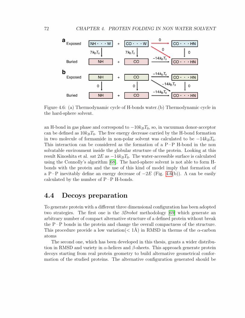
72 CHAPTER 4. PROTEIN FOLDING IN NON WATER SOLVENT
Figure 4.6: (a) Thermodynamic cycle of H-bonds water.(b) Thermodynamic cycle inthe hard-sphere solvent.
an H-bond in gas phase and correspond to −10kBT0, so, in vacuuman donor-acceptorcan be defined as 10kBT0. The free energy decrease carried by the H-bond formationin two molecule of formamide in non-polar solvent was calculated to be −14kBT0.This interaction can be considered as the formation of a P–P H-bond in the nonsolvatable environment inside the globular structure of the protein. Looking at thisresult Kinoshita et al. sat 2E as −14kBT0. The water-accessible surface is calculatedusing the Connolly’s algorithm [68]. The hard-sphere solvent is not able to form H-bonds with the protein and the use of this kind of model imply that formation ofa P–P inevitably define an energy decrease of −2E (Fig. 4.6(b)). Λ can be easilycalculated by the number of P–P H-bonds.
4.4 Decoys preparation
To generate protein with a different three dimensional configuration has been adoptedtwo strategies. The first one is the 3Drobot methodology [69] which generate anarbitrary number of compact alternative structure of a defined protein without breakthe P–P bonds in the protein and change the overall compactness of the structure.This procedure provide a low variation(< 1A) in RMSD in therms of the α-carbonatoms
The second one, which has been developed in this thesis, grants a wider distribu-tion in RMSD and variety in α-helices and β-sheets. This approach generate proteindecoys starting from real protein geometry to build alternative geometrical confor-mation of the studied proteins. The alternative configuration generated should be
4.4. DECOYS PREPARATION 73
defined not an alternative native state, but, in contrast, geometrical native state.This definition is a direct consequence that before the free energy calculation, thereare no relevant information about the solubility and the protein-protein and theprotein-solvent interaction. Complex interaction pattern reviews in the cannot betransposed in this new structure since the completely change of amino acid structure.
Site directed mutagenesis (SDM) developed by Kunkel in 1985 has been widerused to understand the single site change in amino acid sequence on protein sta-bility and solubility [70]. As example Serrano et al. states that a mutations onglycine to alanine depends on the position of the mutated amino acid in the α-helixposition [71]. Glycine is preferred to the amino or the carboxylic terminal part. Asingle mutation can change irremediably the protein stability. The proposed strategyfor the production of alternating configuration have as main purpose to probe theconfiguration landscape and not understand the precise role of amino acid changeas in the site directed mutagenesis. This exploration use as tool the morphometricrationale.
In the aim to build a data bank of misfolded protein, each protein in the Top500database has been sampled [72]. Top 500 database collect proteins with a highquality in resolution, no clashcore presences, no unusual amino acids, no free-atomsrefinement. These proteins structure, on account of this aspects, are used for theRamachandran-plot distributions.
General algorithm can be divided in sub-routines (Fig. 4.7):
Sampling Protein from a database are sampled to generate fragment of N residues.In this step only the α carbon atoms are take into account ().
Compactification Fragment generated are compactificated with Metropolis MonteCarlo procedure.
Checking compactification and reconstruction From the compactification tra-jectory we need the to find the most compactificated protein-like structure frag-ment. To check this feature, the atomistic detail is rebuilt using the referenceprotein.
Analysis Calculate secondary structure and sort the fragments into categories dis-criminated by secondary structure content.
Energy minimization The chosen fragment is submitted to a quick energy mini-mization.
Final analysis and rendering Calculate secondary structure of the minimized struc-ture, analyze, and render protein.
74 CHAPTER 4. PROTEIN FOLDING IN NON WATER SOLVENT
A more detailed scheme is reported in Fig. B.1
4.5 Sampling
Sampling method was performed sequentially for all database proteins (from hereonwards each protein will referred to as Top500protein) to generate a number offragments (from here onwards fragments) of N amino acid residues where N is equalto the the number of residue of the interest protein Nprotein (4ouf, 2pcy). Everyiteration a Top500protein file m is copied in a the work directory. This folder containsthe Top500protein.pdb copied from Top500 proteins database.
Before sampling practice we need to remove unnecessary information from Top500protein file and create a new Top500 protein file composed only by the coordinatesof α-carbon atoms. Atoms in PDB file can be can be defined under two categories,ATOMS and HETATM (heteroatoms) [73]. ATOM keyword is reserved for atomsin standard residues of protein, instead, HETATM is applied to non-standard atomsof protein, like other kinds of groups, such as ligands, solvent, and metal ions. Onlyrarely in Top500 protein files, despite the high quality of the X-ray protein crystalinformations, can be funded uncanonical species of amino acids, different kind ofreagents that intercalate between chains or amino acids vacancy during the crystal-lization process. In .pdb file all this information are defined after the TER keyword.Removing information after this point, and selecting only strings with ATOMS andCA or HETATM and CA is able to prepare a good input file for the sampling algo-rithm. Intrachain HETATM are re-definite as ATOM in the way that compactifica-tion algorithm is able to read it. Only α-carbon coordinates file is named as Top500protein CA. Top500 protein CA file are checked by the number of α-carbon atoms,if smaller than number of residues in candidate N algorithm stops and proceed tothe next Top500 protein in the database. In the other hand, if is bigger, samplingalgorithm select N residues from the first residue j from the amino terminal of theTop500 protein generating the first fragment k. This fragment k will be handled andanalyzed. Regardless of the real accomplishment of this analysis, the next fragmentk+ 1 will be generated selecting the newest first residue adding a shifting value ∆S.
Shifting value ∆S has been choose as 20 residues because this is the typical lengthof α-helix structures. Sampling algorithm stops and restart from a m + 1 Top500protein from the database when the number of remaining residue r in the Top500protein in the working directory is less to the shifting value ∆S.
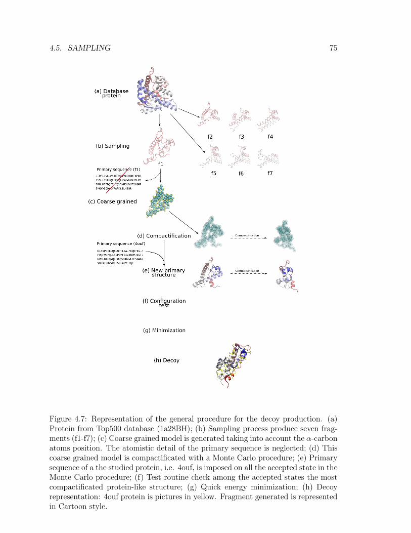
4.5. SAMPLING 75
Figure 4.7: Representation of the general procedure for the decoy production. (a)Protein from Top500 database (1a28BH); (b) Sampling process produce seven frag-ments (f1-f7); (c) Coarse grained model is generated taking into account the α-carbonatoms position. The atomistic detail of the primary sequence is neglected; (d) Thiscoarse grained model is compactificated with a Monte Carlo procedure; (e) Primarysequence of a the studied protein, i.e. 4ouf, is imposed on all the accepted state in theMonte Carlo procedure; (f) Test routine check among the accepted states the mostcompactificated protein-like structure; (g) Quick energy minimization; (h) Decoyrepresentation: 4ouf protein is pictures in yellow. Fragment generated is representedin Cartoon style.
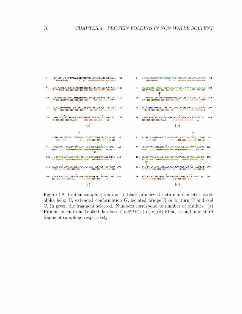
76 CHAPTER 4. PROTEIN FOLDING IN NON WATER SOLVENT
(a) (b)
(c) (d)
Figure 4.8: Protein sampling routine. In black primary structure in one letter code:alpha helix H, extended conformation G, isolated bridge B or b, turn T and coilC. In green the fragment selected. Numbers correspond to number of residues. (a)Protein taken from Top500 database (1a28BH); (b),(c),(d) First, second, and thirdfragment sampling, respectively.

4.6. COMPACTIFICATION 77
4.6 Compactification
The next step is prepare all the preliminary file needed for the compactification.Monte Carlo algorithm for the compactification use as input three files: Top500configuration, primary sequence Top500, primary sequence studied protein. FileTop500 conf is merely a copy of fragment k, primary sequence Top500 is the primarysequence of the fragment k, and primary sequence studied protein is the primarysequence of the interest protein which is stored in the script folder.
The model for the Metropolis Monte Carlo [74] is constituted as a sequences ofN beads with position defined by the α-carbon position (x,y,z) in pdb file, withdiameter σ. For each position is associated a vector (r1, . . . , rN). The consecutivebonds, as n and n + 1, are connected by a fixed bond length b, instead the non-consecutive interact with a square-well potential.
V (SW) =
+∞ for rij < σ
−ε for σ < rij < Rc
0 for r1 > λσ
(4.14)
where rij = |rij| = |rj − ri|, the well width λ − 1 in σ units. This value define therange of interaction Rc = λσ. The ε defines the well depth. Side chain plays arelevant role in protein folding. In this model we take in to account the presence ofthe side chain with N-2 hard sphere of diameter σs. First and last side chain areexcluded in the model. For define the position of the side chains sphere, one definethe tangent Ti and a normal vector Ni as
Ti =ri+1 − ri−1
|ri+1 − ri−1|(4.15)
Ni =ri+1 − 2ri + ri−1
|ri+1 − 2ri + ri−1|(4.16)
and the binormal vector Bi
Bi = Ti ×Ni (4.17)
The side chain sphere is positioned in anti-normal direction with position
r(sc)i = ri −Ni
[(σ + σs)
2
](4.18)
4.7 Checking compactification and reconstruction
Compactification tool should produce a trajectory file where are reported all theaccepted configurations during the Monte Carlo procedure. If compactification had
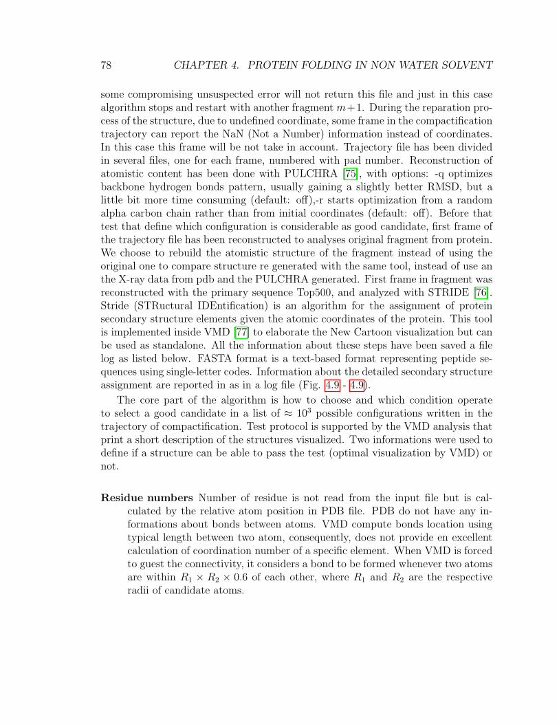
78 CHAPTER 4. PROTEIN FOLDING IN NON WATER SOLVENT
some compromising unsuspected error will not return this file and just in this casealgorithm stops and restart with another fragment m+1. During the reparation pro-cess of the structure, due to undefined coordinate, some frame in the compactificationtrajectory can report the NaN (Not a Number) information instead of coordinates.In this case this frame will be not take in account. Trajectory file has been dividedin several files, one for each frame, numbered with pad number. Reconstruction ofatomistic content has been done with PULCHRA [75], with options: -q optimizesbackbone hydrogen bonds pattern, usually gaining a slightly better RMSD, but alittle bit more time consuming (default: off),-r starts optimization from a randomalpha carbon chain rather than from initial coordinates (default: off). Before thattest that define which configuration is considerable as good candidate, first frame ofthe trajectory file has been reconstructed to analyses original fragment from protein.We choose to rebuild the atomistic structure of the fragment instead of using theoriginal one to compare structure re generated with the same tool, instead of use anthe X-ray data from pdb and the PULCHRA generated. First frame in fragment wasreconstructed with the primary sequence Top500, and analyzed with STRIDE [76].Stride (STRuctural IDEntification) is an algorithm for the assignment of proteinsecondary structure elements given the atomic coordinates of the protein. This toolis implemented inside VMD [77] to elaborate the New Cartoon visualization but canbe used as standalone. All the information about these steps have been saved a filelog as listed below. FASTA format is a text-based format representing peptide se-quences using single-letter codes. Information about the detailed secondary structureassignment are reported in as in a log file (Fig. 4.9 - 4.9).
The core part of the algorithm is how to choose and which condition operateto select a good candidate in a list of ≈ 103 possible configurations written in thetrajectory of compactification. Test protocol is supported by the VMD analysis thatprint a short description of the structures visualized. Two informations were used todefine if a structure can be able to pass the test (optimal visualization by VMD) ornot.
Residue numbers Number of residue is not read from the input file but is cal-culated by the relative atom position in PDB file. PDB do not have any in-formations about bonds between atoms. VMD compute bonds location usingtypical length between two atom, consequently, does not provide en excellentcalculation of coordination number of a specific element. When VMD is forcedto guest the connectivity, it considers a bond to be formed whenever two atomsare within R1 × R2 × 0.6 of each other, where R1 and R2 are the respectiveradii of candidate atoms.
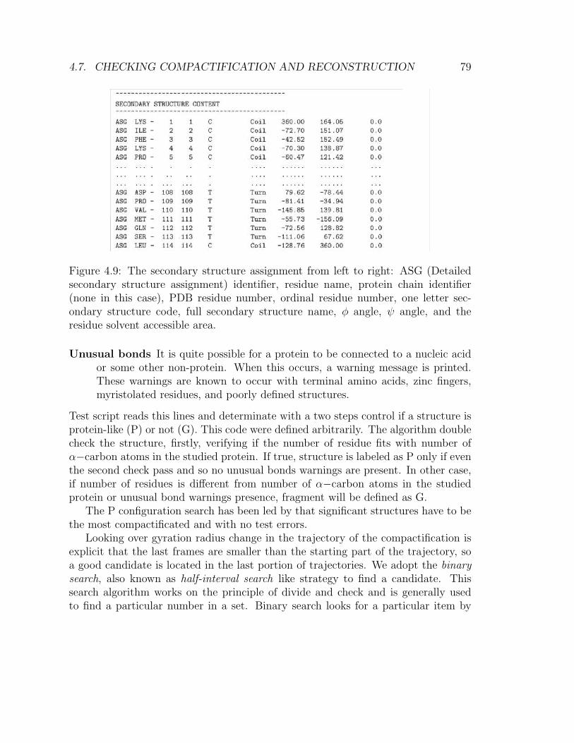
4.7. CHECKING COMPACTIFICATION AND RECONSTRUCTION 79
Figure 4.9: The secondary structure assignment from left to right: ASG (Detailedsecondary structure assignment) identifier, residue name, protein chain identifier(none in this case), PDB residue number, ordinal residue number, one letter sec-ondary structure code, full secondary structure name, φ angle, ψ angle, and theresidue solvent accessible area.
Unusual bonds It is quite possible for a protein to be connected to a nucleic acidor some other non-protein. When this occurs, a warning message is printed.These warnings are known to occur with terminal amino acids, zinc fingers,myristolated residues, and poorly defined structures.
Test script reads this lines and determinate with a two steps control if a structure isprotein-like (P) or not (G). This code were defined arbitrarily. The algorithm doublecheck the structure, firstly, verifying if the number of residue fits with number ofα−carbon atoms in the studied protein. If true, structure is labeled as P only if eventhe second check pass and so no unusual bonds warnings are present. In other case,if number of residues is different from number of α−carbon atoms in the studiedprotein or unusual bond warnings presence, fragment will be defined as G.
The P configuration search has been led by that significant structures have to bethe most compactificated and with no test errors.
Looking over gyration radius change in the trajectory of the compactification isexplicit that the last frames are smaller than the starting part of the trajectory, soa good candidate is located in the last portion of trajectories. We adopt the binarysearch, also known as half-interval search like strategy to find a candidate. Thissearch algorithm works on the principle of divide and check and is generally usedto find a particular number in a set. Binary search looks for a particular item by
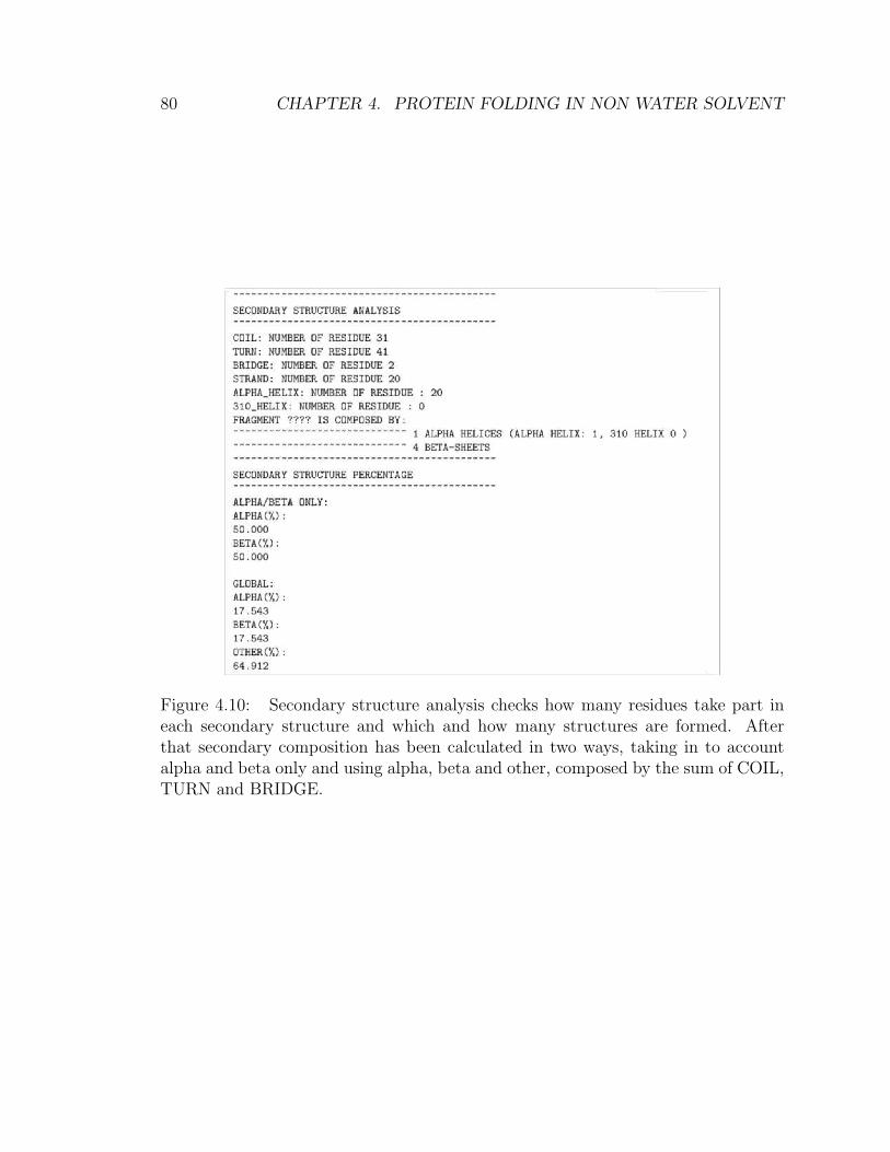
80 CHAPTER 4. PROTEIN FOLDING IN NON WATER SOLVENT
Figure 4.10: Secondary structure analysis checks how many residues take part ineach secondary structure and which and how many structures are formed. Afterthat secondary composition has been calculated in two ways, taking in to accountalpha and beta only and using alpha, beta and other, composed by the sum of COIL,TURN and BRIDGE.

4.7. CHECKING COMPACTIFICATION AND RECONSTRUCTION 81
Figure 4.11: Schematics test example. (a) Unknown trajectory configuration. Firstframe F last frame L are defined by the number of total configuration; (b) Preparativestep. Calculate M, first test define F=P, M=P, and L=G. Mid frame is a protein likeconfiguration. Algorithm checks forward. F and L are recalculated with the followingrules F=M+1 and L=L-1; (c) Starting the real procedure. We define only mid frame.Test define M=G. Algorithm checks backward. F and L are recalculated with thefollowing rules F=F+1 and L=M-1; (d) Test define M=P. Starting jump routine toverify if this P configuration is the larger local P; (e) Jump one step forward until aG state is found; (f) Jump routine J=G. J-1 configuration is straightforwardly thelarger local P.
comparing the middle item of the collection, and, if a match occurs, then the positionof the item is returned. If the middle item is greater than the item, then the itemis searched in the sub-array to the left of the middle item. Otherwise, the item issearched for in the subarray to the right of the middle item. This process continueson the sub-array as well until the size of the subarray reduces to zero. this algorithmto work properly, the data collection should be in the sorted form. Precisely for thisreason we used the idea binary search with the adaptation of case. In trajectoryfile, obviously, we have not information about the test state before the test run ona defined structure, consequently the sorted form is not present. Rather, binarysearch logic has been employ to sample trajectory of compactification in the aim tounderstand which test state is a defined frame and, depending on the test output,algorithm changes the half-interval position.

82 CHAPTER 4. PROTEIN FOLDING IN NON WATER SOLVENT
Algorithm to find a possible candidate works in this way:
1. Frame number in the trajectory define the last frame number variable N (Last),meanwhile, first frame number variable N (First) has been set as one.
2. Mid frame number N (Mid) has been defined as:
N (Mid) = N (First) +
(N (Last) −N (First)
2
)(4.19)
3. Run a first test in the aim to globally check the trajectory the status of firstframe number variable N (First), mid frame number N (Mid), last frame numberN (Last) the result, as P or G, is written in these variables ,N
(First)FT , N
(Last)FT and
N(Mid)FT where FT states for first test. Each test results is printed in the log file
and define a different path in the searching algorithm:
Last frame = P Last frame is P (N(First)FT = P) configuration means that the
most compactificated structure can be read without problem from VMD.
Last frame = G Last frame in G (N(First)FT = G)configuration means that
something wrong happen. Check mid frame number N (Mid).
Mid frame = G when the mid frame is G (N(Mid)FT = G) algorithm start to
search in the first-half (from N (First) to N (Mid)) , after a conclusive output,in the second one of the trajectory (from N (Mid) to N (Last)). Only thebiggest value is accepted. When (N (Mid) = G), this frame is re-analyzedby test function (results is merely the same G). First frame number N (First)
and last frame number N (Last) are redefined and,consequently, mid framenumber N (Last)
N (First) = N (First) + 1 (4.20)
N (Last) = N (Mid) − 1 (4.21)
This test and variables change is looped until test result is P. This op-eration search in the first part of compactification trajectories where therg is certainly too large respect our goal. This logic is forced by the
(N(Mid)FT = G) results and, more likely, the second half of the trajectory is
not usable. Undoubtedly, this P configuration, does not correspond to thelocal larger rg. To score the local P with larger rg easily we check frameby frame moving forward until we find a G. The step before is the largerlocal P configuration for the first half. The second half the trajectory is

4.8. STRIDE ANALYSIS 83
Figure 4.12: Log file showing TEST steps.
explored in the same way taking in to account some modification. Firstframe number N (First) and last frame number N (Last) are redefined as:
N (First) = N (Mid) + 1 (4.22)
N (Last) = N (Last) − 1 (4.23)
This test function and variables change is looped until test result is G.Local P with larger rg is reached frame by frame moving backward untilwe find a P. This frame is the larger local P configuration for the secondhalf. Between and second half configuration algorithm choose the mostcompactificated.
Mid frame = P when the mid frame is P algorithm start to search only inthe second-half.
In Fig. 4.11 is schematized is visualized an test example.
4.8 Stride analysis
After that algorithm finds a candidate, we proceed to categorize fragments in one offive categories using STRIDE:
Type A All-α: protein with 85% of α-helices

84 CHAPTER 4. PROTEIN FOLDING IN NON WATER SOLVENT
Type B 70%α−30%β: protein with a percentage between 85% and 65% of α-helices
Type C 50%α−50%β protein with a percentage between 65% and 45% of α-helices
Type D 30%α−70%β protein with a percentage between 45% and 15% of α-helices
Type E All-β protein with less than 15% of α helices
Files are moved inside a specific percentage folder due the STRIDE analysis, thefile data are collected in a new work folder where name highlight Top500protein ofderivation, the fragment number and is the chosen frame number.
Before a detailed quantitative analysis algorithm attempt to minimize the energyensuring that the system has no steric clashes or inappropriate geometry and im-proves the H-bonds pattern in decoys. The simulations were performed in periodiccubic box with a distance between the solute and the box of 1 nm (approximately6 nm and 7500 water molecules). The integrator algorithm for energy minimizationwas set as steep descent. The minimization is converged when the max force issmaller than 100 kJ mol1nm1, maximum step size in nm 0.01 nm and the maximumnumber of steps was set as 50000. Frequencies to update the neighbor list (and thelong-range forces, when using twin-range cut-off) were updated every step. Bondsand angles were not constrained.
Minimized structures were tested to check if the configuration contains unusualbonds or number of residues were different as arranged beforehand. In negative casealgorithm analyze the structure even before the minimization. In the word directorycan be written three possible folder, in function of the minimization routine. If theminimization fails or test has been settled as negative (G), non minimized fragmentis goes to the rendering and analysis procedure.
Analysis routine calculate and compare: the native protein gyration radius rNativeg ,
fragment gyration rFragmentg , RMSD between native protein and fragment, and the
variation between gyration radii of native protein and fragment ∆. There are twoatom selections needed to do an RMSD computation in VMD, the list of atoms tocompare in both molecules. RMSD is define as:
RMSD =
√√√√ 1
N
N∑i=1
δ2i (4.24)
where δi is the distance between atom i and either a reference structure or the meanposition of the N equivalent atoms. The first atom of the first selection is comparedto the first atom of the second selection. To fit structures α-carbon atoms were

4.9. RESULTS 85
TYPE 〈rg〉 (A) rMing -rMax
g (A) 〈RMSD〉 (A) RMSDMin-RMSDMax (A) 〈∆rg〉 (%) ∆rMing -∆rMax
g (%)
A 14.19 11.04-21.82 61.45 51.16-80.00 −1.10 −23.07-52.08B 13.98 11.56-19.40 60.86 52.07-79.39 −2.54 −19.39-35.20C 14.42 11.77-21.61 62.02 52.14-77.30 0.51 −17.97-50.62D 14.18 12.18-19.36 61.45 54.59-73.62 −1.14 −15.09-34.95E 13.94 11.89-22.88 61.44 54.18-92.47 −2.81 −17.11-59.47
Table 4.1: 4ouf protein statistics for types A-E.average gyration radius 〈rg〉,minimum-maximum gyration radius (rMin
g and rMaxg ), averages RMSD, minimum-
maximum RMSD (RMSDMin and RMSDMax), average gyration radius variation〈∆rg〉, minimum-maximum gyration radius variation (∆rgMin and ∆rMax
g ).
choose as comparative coordinate. The actual order is identical to the order fromthe input PDB file. Returns the radius of gyration of atoms in selection using thegiven weight. The radius of gyration is computed as
r2g =
(∑n
i=1 wi(ri − r)2)
(∑n
i=1 wi)(4.25)
where ri is the position of the ith atom and r is the weighted center
4.9 Results
All decoys generated for 4ouf and 2pcy have been explored in meaning of gyrationradius, RMSD, alpha-beta secondary structure percentage,and gyration radius vari-ation respect of the studied protein ( r4ouf
g = 14.352 A and r2pcyg = 12.342 A).
For the 4ouf protein we obtained 1048 protein distributed as follows: for thetype A 564 structures, type B 279 structures, type C 84 structures, type D 61structures,and type E 60 structures. This proteins have been explored in meaningas
Algorithm generate 1294 fragments of which 717 for the type A protein decoys,276 for type B protein decoys , 105 for protein decoys type C,103 for protein decoystype D, and 93 type for protein decoys E.
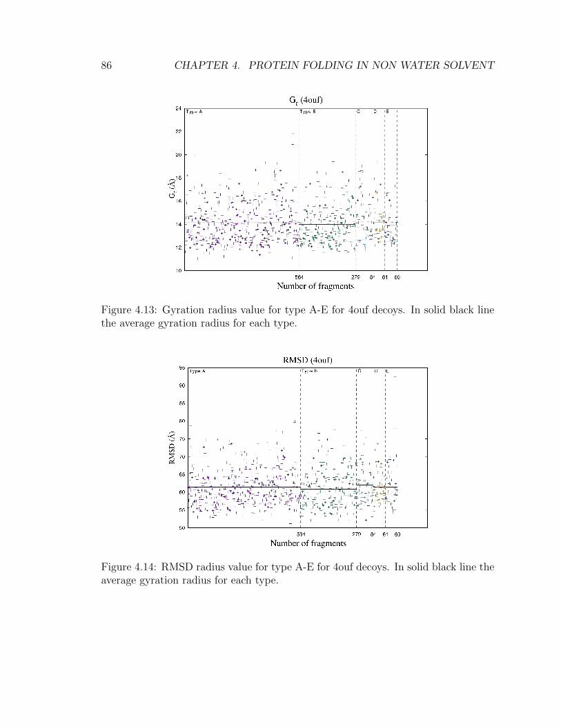
86 CHAPTER 4. PROTEIN FOLDING IN NON WATER SOLVENT
Figure 4.13: Gyration radius value for type A-E for 4ouf decoys. In solid black linethe average gyration radius for each type.
Figure 4.14: RMSD radius value for type A-E for 4ouf decoys. In solid black line theaverage gyration radius for each type.

4.9. RESULTS 87
Figure 4.15: Variation in gyration radius value for type A-E for 4ouf decoys. In solidblack line the average gyration radius for each type.
Figure 4.16: α-β percentage for 4ouf decoys generated.

88 CHAPTER 4. PROTEIN FOLDING IN NON WATER SOLVENT
TYPE 〈rg〉 (A) rMing -rMax
g (A) 〈RMSD〉 (A) RMSDMin-RMSDMax (A) 〈∆rg〉 (%) ∆rMing -∆rMax
g (%)
A 14.19 10.16-20.83 38.69 35.88-42.64 8.12 −17.69-68.78B 13.30 10.64-18.30 38.66 36.41-42.61 7.7 −13.78-48.28C 14.03 10.91-22.59 38.93 36.19-42.10 13.69 −11.57-83.01D 13.69 10.89-20.92 38.87 36.57-43.58 10.94 −11.74-69.56E 13.12 11.30-20.27 38.68 36.89-40.48 6.29 −8.40-64.28
Table 4.2: 2pcy protein statistics for types A-E.average gyration radius 〈rg〉,minimum-maximum gyration radius (rMin
g and rMaxg ), averages RMSD, minimum-
maximum RMSD (RMSDMin and RMSDMax), average gyration radius variation〈∆rg〉, minimum-maximum gyration radius variation (∆rgMin and ∆rMax
g ).
Figure 4.17: Gyration radius value for type A-E for 2pcy decoys. In solid black linethe average gyration radius for each type.

4.9. RESULTS 89
Figure 4.18: RMSD radius value for type A-E for 2pcy decoys. In solid black linethe average gyration radius for each type.
Figure 4.19: Variation in gyration radius value for type A-E for 4ouf decoys. In solidblack line the average gyration radius for each type.
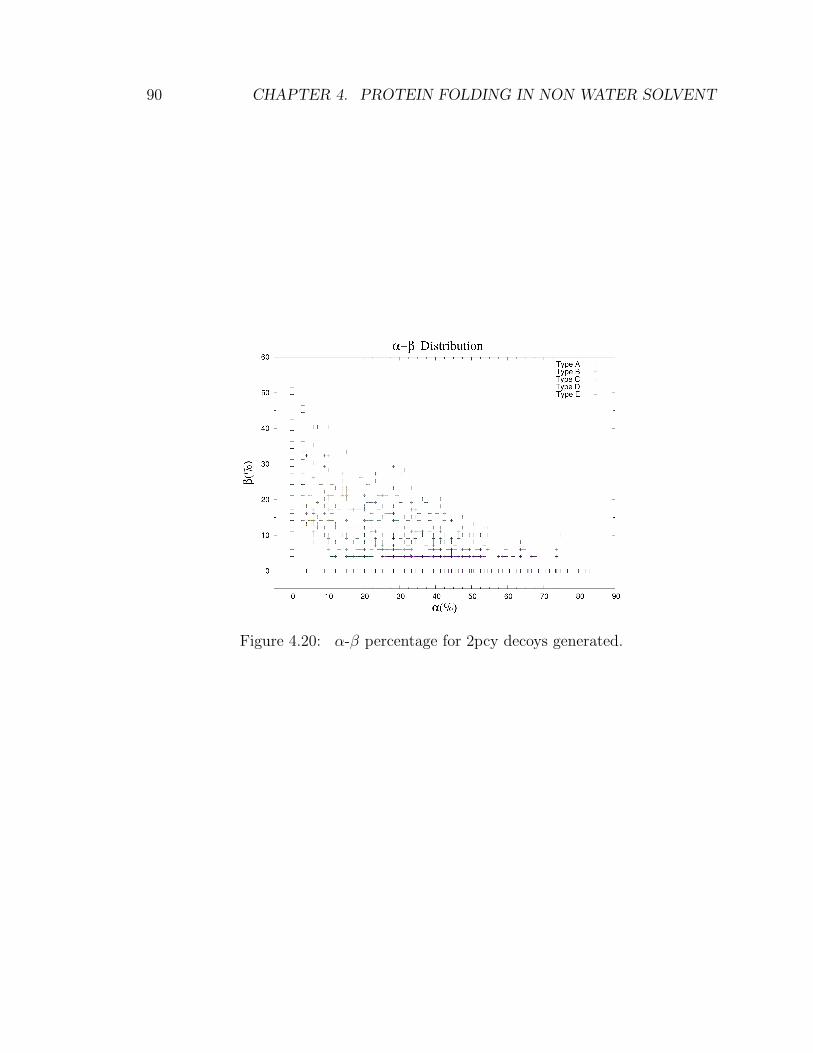
90 CHAPTER 4. PROTEIN FOLDING IN NON WATER SOLVENT
Figure 4.20: α-β percentage for 2pcy decoys generated.
Conclusion and perspective
The aim of the of this thesis was to understand the effect of solvent specificities onthe stability of a specific protein. Water is a fundamental solvent of nearly, if notall, biological processes. Water was in fact selected by nature to this aim in viewof this extraordinary properties, as briefly described in Chapter 1. Several studieshave underlined the importance of considering other solvents to understand how livefirst emerged on Earth under probiotic conditions, as well as, how life could existon other planets. Motivated by this studies, tackled the problem using two differentapproaches. In the first approach, we compute explicitly the change in free energywhen specific amino acids are brought from a gas phase to water. To this aim, weused thermodynamic integration, a versatile tool that could be adapted to differentsolute, as full protein, and different solvent, as an apolar solvent. The results ofthis first part could be used to test the reliability of an alternating approach, calledmorphometric approach, to the calculation of this free energy change used in thesecond part.
The analysis of the data generated from the thermodynamic integration calcu-lations, using gromos54a7, implemented with the ATB optimized structure, non-bonded and bonded interaction, produced results in general consistent with the ex-perimental and calculated values (Figs. 3.1-3.2). Respect of the value calculated byVilla et al. [51] customized gromos54a7 with Automated Topology builder (ATB) fea-tures results more able to fit the experimental data. In comparison with free energyvalue available from ATB the gromos54a7 results slightly more precise. This precisioncould be effered to a most modern forcefield or the more precise feature of GRO-MACS version. These lineup has been used to understand, using the variation of freeenergy in function of λ and the cumulative free energy that returns the ∆GSolv, thenon-bonded interaction between solvent and compound. As default the λ steps havebeen set as 20 (∆λ = 0.05). Amino acid have several different chemical characteristicand, consequently, define different results depending on the chemical group-solventinteraction during the decoupling. Using the Bennet’s acceptance ratio and ancillarydata generated we were able to refine the λ value as needed to improve precision
91

92 CHAPTER 4. CONCLUSION AND PERSPECTIVE
in particular simulation runs. This hypothesis has been confirmed several trendingpattern evaluable in change of free energy as function of λ, and by the evidence thatchemically correlated amino acids generated similar data. As stated before, the mainintent of this analysis was not the validation, or a comparative study on a force fieldrespect to another. Results in this first part of the thesis can be defined as a startingpoint to explore the free energy decoupling ”fingerprints” of a particular chemicalgroup in water, and the respective interaction with other polar solvent or non polaras ethanol or cycloehexane, respectively. Exhaustive understanding of these inter-action could have a pivotal role in the comprehension of contribute of single aminoacid in numerical methods free energy calculation. Collimating this results witha parallel study of the compound in other solvent results could able to clarify thetransfer free with mixed solvent phase as from low dielectric, as cycloehexane, tohigh dielectric, as water. The understanding of these phenomena in molecular dy-namic permit to simulate biological mixed solvent as the integral membrane proteins.Further research, could focus on the analysis in computational and experimental inseveral solvent, of little peptide, with different amino acid composition in the way tomore comprehend the interaction. Beside the molecular dynamics calculation theselittle peptide could be used, subsequently, in morphometric method proposed in thesecond part.
The second part of the thesis take on the free energy of solvation explorationfrom a non numerical methods, strictly considering the work done, standpoint. Thedevelopment of a collection of protein, with different amount of secondary structurefrom an unique sequence of amino acids, the primary structure, has been requiredto explore the configuration phase with aim to find the free energy difference respectof the native state of the protein studied. Protein with the same primary struc-ture but different geometry are called decoys. The distinctiveness of this methods isthat use pre-existing native structure, or more precisely the three-dimensional back-bone structure, to generate possible stable conformation. Proposed morphometriccalculation of free energy calculation needs less computational time than moleculardynamics and can be used to scan large protein population. Beside the hypothesisto discover a different native state, or a configuration with a similar free energy ofsolvation, this collection can be used to investigate qualitatively alternative foldingin different solvents. Algorithm proposed has been able to generate 1048 alternativeconfiguration for the 4ouf as following reported: 564 structures all-α, 279 70%-α,84 50%-α, 61 30%-α, 60 all-β; and 1294 alternative state for 2pcy of which 717 all-α, 276 70%-α, 105 50%-α, 103 30%-α, and 93 all-β. The minimum and maximumRMSD values for 4ouf and 2pcy are 51.16 A to 92.47 A and 35.88 A to 43.58 A respec-tively, producing a wide change in geometry as expected. The proposed routine, even

93
thought generated a generous amount of protein decoys, could be surely improvedas the efficiency of decoys generated. Using different sampling logic or acceptancecould be possible generate more precise restraint so that it can be possible range thedecoys variety.

94 CHAPTER 4. CONCLUSION AND PERSPECTIVE

Appendix A
Experimental methods
A.1 X-ray crystallography
This technique is based on the analysis of the atomic and molecular structures ofa crystal using diffraction pattern generated by the scattering of a electromagneticradiation, in this case the x-ray. The X-ray, photons with a wavelength λ rangedbetween 0.1 and 100 A, are generated colliding high accelerated electrons on a tung-sten surface. The impact generate photons by Bremsstrahlung effect. In a regulararray of atoms, where the scatter are due by the atom’s electron, X-rays scatteringproduces a regular array of spherical waves These waves can cancel out other wavesthrough destructive interference or add constructively in a few specific directions,determined by Bragg’s law:
2d sin θ = nλ (A.1)
The bragg’s law is correlated with the vector of scattering K where the module isrelated with the scattering angle θ:
|K| = 1
π
sin θ
λ(A.2)
and results included between 0 and 1/πλ.The X-ray crystallography determine the density of charge ρ(r) throughout the
crystal, where r represents the three-dimensional position vector within the crystal.X-ray scattering is used to collect data about its Fourier transform F (K). From thisvalue is possible calculate the density defined in real space, using the formula
F (K) =
∫d3rρ(r) exp [−iKr] (A.3)
95
96 APPENDIX A. EXPERIMENTAL METHODS
ρ(r) =1
(2π)3
∫dKF (K) exp [iKr] (A.4)
The structure factor F (K) is a complex number, therefore:
F = |F |2 exp[iφ] (A.5)
F = FR + iFi (A.6)
The intensity I(K) calculated by the instrument is real number and is the productbetween the structure factor F (K) and his complex conjugate F ∗(K)
I(K) = F (K)F ∗(K) = |F |2 (A.7)
From the structure factor is not possible calculate the phase parameter. Protein crys-tallization is predominantly carried out in water. Protein crystallization is generallyconsidered challenging due to the restrictions of the aqueous environment, difficultiesin obtaining high-quality protein samples, as well as sensitivity of protein samplesto temperature, pH, ionic strength, and other factors. Proteins vary greatly in theirphysiochemical characteristics, and so crystallization of a particular protein is rarelypredictable
After the crystallization, to find the unknown phase, isomorphic crystals needsto be preprepared. This kind of crystal are generated by diffusion of heavy atoms bya regent in the protein crystal. Silver nitrate (AgNO3) is able to bind the with thethiol ( –SH). The structure factor of the isomorphic protein crystal FPH(K) is thesum of the protein structure factor FP (K) and the heavy atoms FH(K):
FPH(K) = FP (K) + FH(K) (A.8)
The amplitude |F (K)| can be approximated using the difference between the differ-ence between the isomorphic crystal and the real protein crystal. The Patterson canbe calculated by:
∆P =1
V
∑K
||FPH − |FP ||2 exp[iKR] (A.9)
where R is the atoms position. All the value of FP are arranged on a circumferenceof radius |FP | centered in the origin. In the same way, all the value of FPH arearranged on a circumference of radius |FPH | centered in the origin. The intersectionpoints between these circumference that fulfill the equation are two phase φa and φb.To choose the right phase can be prepared more isomorphic crystal with a severaldifferent heavy atoms. According with the resolution achieved different details canbe defined,

A.2. CALORIMETRY 97
Resolution Details
6 A α-helix appear like sticks.The protein can be divide in sub-uni.
3 A The backbone can be defined2.5 A Almost all side chain is visible.
The carbonyl of the peptide bond permit.to define the plane orientations
1.5 A All atom are visible
Table A.1: Resolution and details achieved in X-ray diffraction.
A.2 Calorimetry
As Anfinsen shown, protein folding is reversible thermodynamic processes. To studythis fold-unfold process several experimental ultra-sensitive technique has been de-veloped.
A.2.1 Differential scanning calorimetry
The differential scanning calorimetry, or DSC is a thermo analytical procedure thatis based on the comparison about the amount of heat necessary to maintain at thesame temperature a interest sample and a reference. The difference in temperaturein a DSC experiment is curve of heat in function of temperature. Working in isobariccondition the change in heat is equal to the change in enthalpy.(
dQ
dT
)P
=dH
dT(A.10)
the entalpy can be obtained integrating
∆Hsample =
∫dHsample
dTdT (A.11)
Cprot = C(ref)prot
(dQdT
)P(
dQref
dT
)P
m
mref
(A.12)
where m and mref are the masses of the sample and the reference, respectively.

98 APPENDIX A. EXPERIMENTAL METHODS
A.2.2 Isothermal titration calorimetry
The isothermal titration calorimetry, or ITC is a used to determine the thermody-namic parameters of interactions in solution. This kind of routine is used to studythe binding energy of little ligands in macromolecules, Like the energy of interac-tion of compound, like a drug, with an active site. In protein folding studies thetitration is intended to unfold the protein. The experiment runs into a titration ofa solution by a titrating, monitoring heat released or absorbed by the reaction. Theinstrument is composed by identical cells made of thermally conducting and chem-ically inert material. This cells are protected by an adiabatic jacket. Thermopile,an electronic device that converts thermal energy into electrical energy, are used todetect temperature differences between the reference cell and the sample cell. Thereference cell, filled with buffer or water, Prior to addition of ligand, is preheat ap-plying a constant power. Measurements consist of power required to maintain equaltemperatures between the sample and reference cells. This plot is time dependent.Repeating the experiment at different temperature is possible calculate the sampleheat capacity. From a typical plot of CP can be obtained several information. Thepeak area is the change in enthalpy derived by the protein unfolding. From theshape of the peaks can be calculated the van’t Hoff enthalpy ∆Hvan′tHoff . The van’tHoff equation calculate the variation in the equilibrium constant Keq of a reactionto the change in temperature T , given the standard enthalpy change, ∆H−−, for theprocess.
d lnKeq
dT= −∆H−−
R. (A.13)
From the isothermal titration calorimetry data the van’t Hoff entalpic can be rewrit-ten as:
∆Hvan′tHoff =4RT 2
t C(max)p
∆Hcalc
(A.14)
where Tt is the transition temperature between the folded and the unfolded state,R is the universal constant of gas C
(max)p is the maximum heat capacity and ∆Hcalc
is the area of the peak in the transition. In the event that the van’t Hoff enthalpy∆Hvan′tHoff and the calculated change in enthalpy ∆Hcalc, so the change in free energyis zero, is possible to calculate the folding entropy.
∆H = T∆S + V∆P (A.15)
and
∆Q = T∆S (A.16)
A.2. CALORIMETRY 99
definifg the entropy and enthalpy difference between the denature state and thenative, so the contribute due to the unfolding process, as ∆U
NS(Tt) ∆UNH(Tt), respec-
tively, the unfolding s entropy ∆UNS(Tt) can be written as:
∆UNS(Tt) =
∆UNH(Tt)
Tt(A.17)
Know the various heat capacity at different temperature, the entropy and enthalpyof folding can be calculated in function of the temperature T :
∆UNH(T ) = ∆U
NH(Tt) +
∫ T
Tt
∆UNCp(T
′)dT ′ (A.18)
and
∆UNS(T ) =
∆UNH(Tt)
Tt+
∫ T
Tt
∆UNCp(T
′)d lnT ′ (A.19)
This procedure is dependent by the experiment condition therefore is possible obtaindifferent folding temperature. Changing reducing agent or pH can lead to differentresults. The dependence of the temperature of transition Tt with the pH can be usedto calculate the amount of proton species released during the experiment.
∆vt = −∆Hcalc(Tt)
2.303RT 2t
dTtd(pH)
(A.20)

100 APPENDIX A. EXPERIMENTAL METHODS

Appendix B
General algorithm for decoysconstruction
101
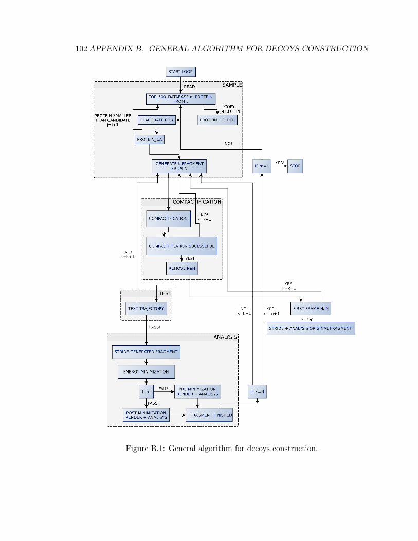
102 APPENDIX B. GENERAL ALGORITHM FOR DECOYS CONSTRUCTION
Figure B.1: General algorithm for decoys construction.

103
Figure B.2: Test algorithm procedure.

104 APPENDIX B. GENERAL ALGORITHM FOR DECOYS CONSTRUCTION

Bibliography
[1] D. Schulze-Makuch; S. Haque; M. R. de Sousa Antonio, D. Ali, R. Hosein, Y. C.Song, J. Yang, E. Zaikova, D. M. Beckles, E. Guinan, H. J. Lehto,S. J. Hallam.Astrobiology, Volume 11, Issue 3, 241-258 (2010).
[2] Cox) D. L. Nelson, M. M. Cox ”Lehninger Principles of Biochemistry”.W.H.Freeman & Co Ltd (2013)
[3] R. Horton, L. A. Laurence G. Scrimgeur M. Perry D.Rawn ”Principles of Bio-chemistry” fourth edition Pearson Education (2006)
[4] S. Freeman ”Biological Science” Prentice Hall; 2nd Edition edition (2005)
[5] K. Bosco, R. Brasseur. BMC Structural Biology, 5, 14 (2005).
[6] L. Pauling, R. B. Corey, H. R. Branson. Proceedings of the National Academyof Sciences, 37 (4) 205-211 (1951)
[7] G. N. Ramachandran, C. Ramakrishnan, V. Sasisekharan. Journal of MolecularBiology. 7: 95–9 (1963)
[8] https://commons.wikimedia.org/wiki/File%3AAlpha_helix_neg60_
neg45_sideview.png
[9] https://commons.wikimedia.org/wiki/File%3AAlpha_helix_neg60_
neg45_topview.png
[10] https://commons.wikimedia.org/wiki/File%3A3_10_helix_neg49_neg26_
sideview.png
[11] https://commons.wikimedia.org/wiki/File%3A310_helix_topview.png
[12] https://commons.wikimedia.org/wiki/File%3APi_helix_neg55_neg70_
sideview.png
105
106 BIBLIOGRAPHY
[13] https://commons.wikimedia.org/wiki/File%3APi_helix_topview.png
[14] P.Y. Chou,G.D Fasman. Biochemistry. 13 (2): 222–245 (1974).
[15] J. Garnier, D. J. Osguthorpe, B Robson. J Mol Biol 120:97-120 (1978).
[16] M. Sela, F. H. Jr. White, C. B. Anfinsen. Science. 125 (3250): 691–692 (1957).
[17] C. Levinthal, J. Chem. Phys 65, 44 (1968).
[18] M. Mezard, G. Parisi, and M. Virasoro. ”Spin Glass Theory and Beyond”. WorldScientific, Singapore (1987).
[19] C. Branden, J. Tooze. ”Introduction to Protein Structure”. New York: GarlandPublishing (1991).
[20] J. D. Bryngelson, P. G. Wolynes. 84:7524-7528 (1987).
[21] J. D. Bryngelson, J. N. Onuchic, N. D. Socci, P. G. Wolynes. Proteins, 21:167–195. (1995)
[22] R. Dawkins ”The Blind Watchmaker”. New York: W. W. Norton & Company,Inc (1986).
[23] P. E. Leopol, M. Montal, J. N. Onuchic. Proc. Natl. Acad. Sci. USA. 89 (18):8721–5. (1992).
[24] D. Baker, Nature 405, 39 (2000).
[25] P. G. Wolynes, J. N. Onuchic, and D. Thirumalai, Science 267, 1619 (1995).
[26] K. A. Dill and H. S. Chan, Nat. Struct. Biol. 4, 10 (1997).
[27] P. C. Hiemenz. ”Principle of colloids and surface chemistry”, Second editionMarcel Dekker, New York (1986).
[28] R. L. Baldwin,G. D. Roseg. Curr Opin Struct Biol. 23 (1): 4–10 (2013).
[29] K. A. Dill. Biochemistry. 24 (6): 1501–9 (1985).
[30] B. W. Matthews, H. Nicholson, W. J. Becktel. Proc. Natl. Acad. Sci. USA.84(19), 6663–6667 (1987).
[31] D. Shortle. FASEB J. 10(1):27-34 (1996).

BIBLIOGRAPHY 107
[32] J Mol Biol. 20;238(5):777-93 (1994).
[33] R. Ludwig. Angewandte Chemie International Edition, 40: 1808–1827 (2001).
[34] W. Kauzmann. Adv. Protein Chem, 14, 1–63 (1959).
[35] J. Chen, W. E. Stites. Biochemistry 40, 15 280–15 289 (2001).
[36] C. N. Pace. Biochemistry 40, 10–313 (2001).
[37] T. J. Taylor, I. I. Vaisman. BMC Structural Biology, 10(Suppl 1):S5 (2010).
[38] C. N. Pace, S. Trevino, E. Prabhakaran, J. M. Scholtz (2004). PhilosophicalTransactions of the Royal Society B: Biological Sciences, 359(1448), 1225–1235(2004).
[39] B. J. Alder and T. E. Wainwright. The Journal of Chemical Physics 27, 1208(1957).
[40] D. Fraankel, B. Smit. ”Understanding molecular simulation. From algorithm toapplications” Academic press, USA (2002)
[41] A. R. Leach ”Molecular modelling. Principles and applications” second edition,Person Education Limited, England (2001)
[42] M. Abraham, B. Hess, D. van der Spoel, E. Lindahl. ”GROMACS ReferenceManual, Version 2016” Department of Biophysical Chemistry, University ofGroningen (2016)
[43] N. Metropolis, A. Rosenbluth, M. Rosenbluth, A. Teller, and E. Teller, J. Chem.Phys. 21, 1087 (1953).
[44] J. G. Kirkwood. J. Chem. Phys., 3:300-313 (1935).
[45] C. H. Bennett. Journal of Computational Physics 22 : 245–268 (1976)
[46] S. Bruckner, S. J. Boresch. Comput. Chem., 32: 1303–1319 (2011)
[47] https://atb.uq.edu.au/
[48] K.B. Koziara, M. Stroet, A. K. Malde, A. E. Mark. Journal of Computer-AidedMolecular Design, 28, 221-233 (2014)

108 BIBLIOGRAPHY
[49] N. Schmid, A. P. Eichenberger, A. Choutko, S. Riniker,M. Winger,A. E. Mark,W.F van Gunsteren. European Biophysics Journal, 40, 843-856 (2011).
[50] A.K. Malde, L. Zuo, M. Breeze, M. Stroet,D. Poger,P. C. Nair, C. Oostenbrink,A. E. Mark. Journal of Chemical Theory and Computation, 7(12), 4026-4037(2011).
[51] A. Villa, A. E. Mark. J. Comput. Chem., 23: 548–553. (2002).
[52] C. Jaeeon, M. L. Abraham, S. I. Sandler. The Journal of Physical Chemistry B111 (8), 2098-2106 (2007).
[53] R. Wolfenden, L. Andersson, P. M. Cullis, and C. C. B. Southgate. Biochemistry.20 (4), 849–855 (1981).
[54] R. C. Rizzo, T. Aynechi, D. A. Case, I. D. Kuntz†. Journal of Chemical Theoryand Computation 2 (1), 128-139 (2006).
[55] P. D. Thomas, K. A. Dill. Proceedings of the National Academy of Sciences 93(21) 11628-11633 (1996)
[56] B. Parka, M. Levitt. Journal of molecular biology. 258, (2) 367-92 (1996).
[57] J. Zhu, Q. Zhu, Y. Shi, H. Liu, Proteins, 52: 598–608 (2003).
[58] M. Kinoshita, J. Chem. Phys. 128, 024507 (2008).
[59] T. Yoshidome and M. Kinoshita, Phys. Chem. Chem. Phys. 14, 14554 (2012).
[60] M. Kinoshita, Biophys. Rev. 5, 283 (2013).
[61] H. Oshima and M. Kinoshita, J. Chem. Phys. 142, 145103 (2015).
[62] T. Hayashi, S. Yasuda, T. Skrbic, A. Giacometti, and M. Kinoshita. The Journalof Chemical Physics 147, 125102 (2017).
[63] P. M. Konig, R. Roth, and K. R. Mecke. Phys. Rev. Lett. 93, 160601 (2004).
[64] R. Roth, Y. Harano, and M. Kinoshita. Phys. Rev. Lett. 97, 078101 (2006).
[65] C. Das, S. Roy, S. Namjoshi, C.S. Malarkey, D.N. Jones, T.G. Kutateladze, M.E.Churchill, J.K. Tyler. Proc. Natl. Acad. Sci. USA 111: E1072-E1081 (2014).
BIBLIOGRAPHY 109
[66] T.P Garrett, D.J. Clingeleffer, J.M. Guss, S.J. Rogersm, H.C. Freeman.J.Biol.Chem. 259: 2822-2825 (1984).
[67] B. Lee, F. M. Richards. J Mol Biol 55(3):379-400 (1971).
[68] M. L. Connolly, J. Am. Chem. Soc. 107, 1118 (1985).
[69] H. Deng, Y. Jia, and Y. Zhang, Bioinformatics 32, 378 (2016).
[70] T. A. Kunkel Proceedings of the National Academy of Sciences. 82 (2): 488–92(1985).
[71] L. Serrano, L. J. Neira, J. Sancho, A. R. Fersht. Nature. 1992 Apr 2;356(6368):453-5 (1992).
[72] http://kinemage.biochem.duke.edu/databases/top500.php
[73] J. Callaway, M. Cummings, B. Deroski, P. Esposito, A. Forman, P. Langdon, M.Libeson, J. McCarthy, J. Sikora, D. Xue, E. Abola, F. Bernstein, N. Manning,R. Shea, D. Stampf, and J. Sussman. Brookhaven National Laboratory (1996).
[74] T. Skrbic, T. X. Hoang, A. Maritan, J. R. Banavar, and A. Giacometti. (un-published)
[75] P. Rotkiewicz, J. Skolnick. 29(9):1460-1465 (2008).
[76] D. Frishman, P. Argos. Proteins 23(4):566-79 (1995).
[77] W. Humphrey, A. Dalke, K. Schulten. J. Molec. Graphics, 14, 33–38 (1996).


![PROTEIN ENGINEERING. Protein engineering-Why? Enhance stability/function under new conditions –temperature, pH, organic/aqueous solvent, [salt] Alter.](https://static.fdocuments.in/doc/165x107/56649e0e5503460f94af78bb/protein-engineering-protein-engineering-why-enhance-stabilityfunction-under.jpg)


