Computational Modelling of Unsteady Rotor Effects

Duncan McNae – PhD candidate

Professor J Michael R Graham

Summary

Background

Numerical Model

Results

Ongoing Work

Summary

Background

Numerical Model

Results

Ongoing Work

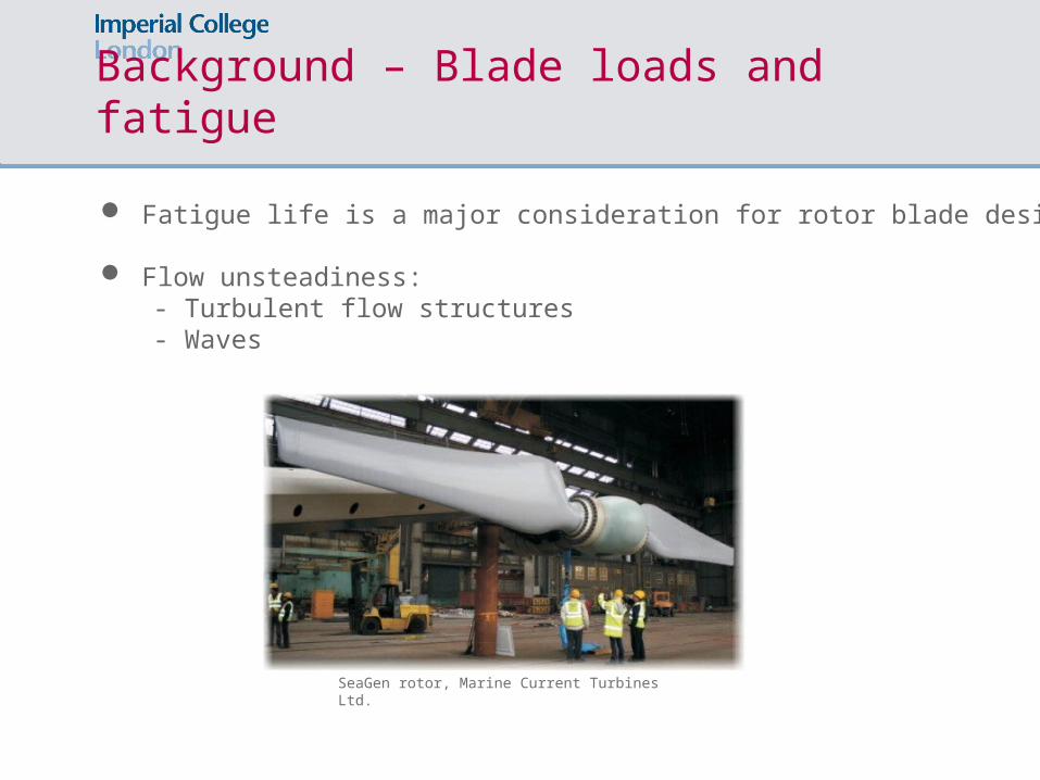
Background – Blade loads and fatigue

SeaGen rotor, Marine Current Turbines Ltd.

Fatigue life is a major consideration for rotor blade design

Flow unsteadiness:- Turbulent flow structures- Waves

Background – Unsteady Flow Effects

Key principle:

– Dynamic Inflow Fluctuations in flow speed cause changes in the loading on

the rotor, and therefore the strength of vorticity trailing into the wake is not constant. The induced velocity field takes time to develop as a result.

Burton et alBurton et al. 2001

Summary

Background

Numerical Model

Results

Ongoing Work

Numerical Model

Numerical modelling techniques:

Blade Element Momentum Theory (BEM)

Potential Flow / Vortex Methods

Computational Fluid Dynamics (CFD)

Numerical Model

Numerical modelling techniques:

Blade Element Momentum Theory (BEM)

Potential Flow / Vortex Methods

Computational Fluid Dynamics (CFD)

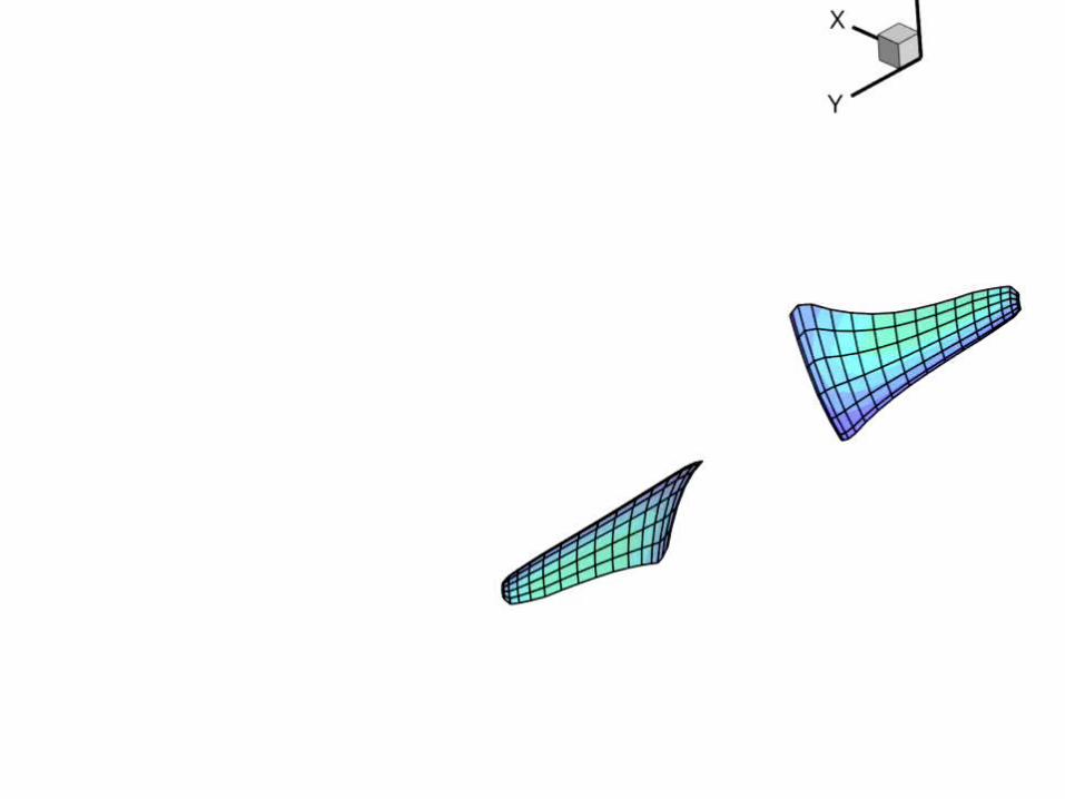
Numerical Model – The Vortex Lattice Method

The blade–wake system can be represented by a lattice of “vortex rings”, or “panels”. This concept is derived from potential flow theory.

Vortex rings are distributed on the blade camber line, and the wake panels are free – they move with the flow.

A system of equations is formed with the use of a zero-flow-normal boundary condition at the center of each panel – the “collocation points”.

Representation of a vortex ringΓ = circulation strength

Biot–Savart Law

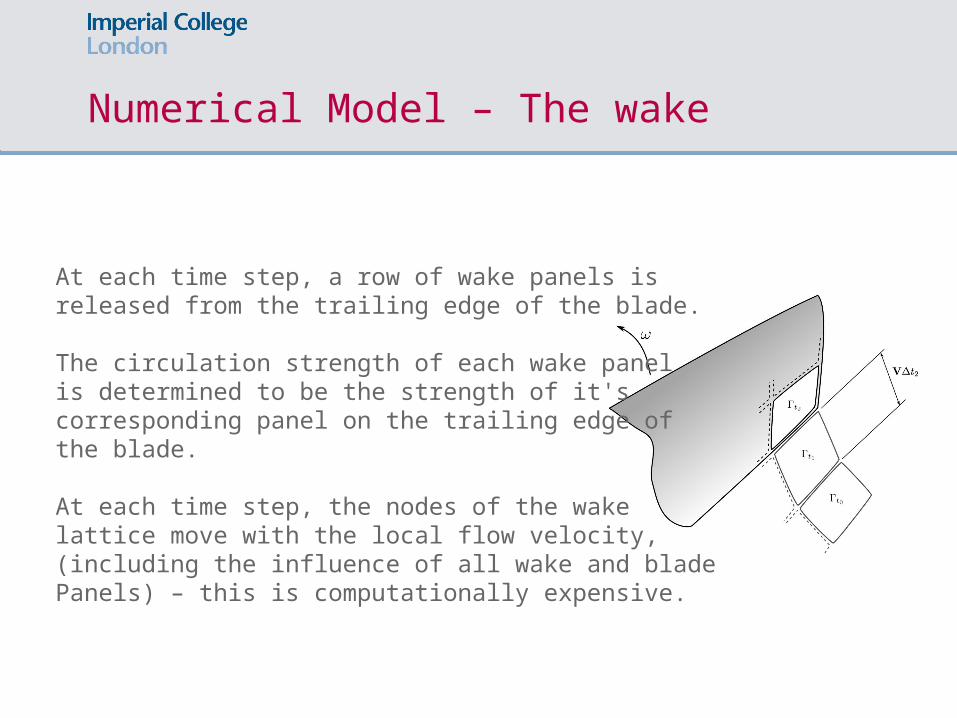
Numerical Model – The wake

At each time step, a row of wake panels isreleased from the trailing edge of the blade.

The circulation strength of each wake panel is determined to be the strength of it's corresponding panel on the trailing edge of the blade.

At each time step, the nodes of the wakelattice move with the local flow velocity,(including the influence of all wake and bladePanels) – this is computationally expensive.

Numerical Model – Loads

The loading contribution of each panel is calculated using the following:

This is a form of the unsteady Kutta-Joukowski equation.

Numerical Model – Validation

Validation of the unsteady vortex lattice method (VLM):

Flat plate steady case

Flat plate unsteady

Rotor

Numerical Model – Validation

For a simple flat plate wing case (AR=8), the VLM has been compared with “Tornado”, which is a similar program that has been developed for aircraft design.

Numerical Model – Validation

Unsteady flat plate oscillations, vs Theodorsens theory:

Numerical Model

– Coefficient of Power:

– Coefficient of Thrust:

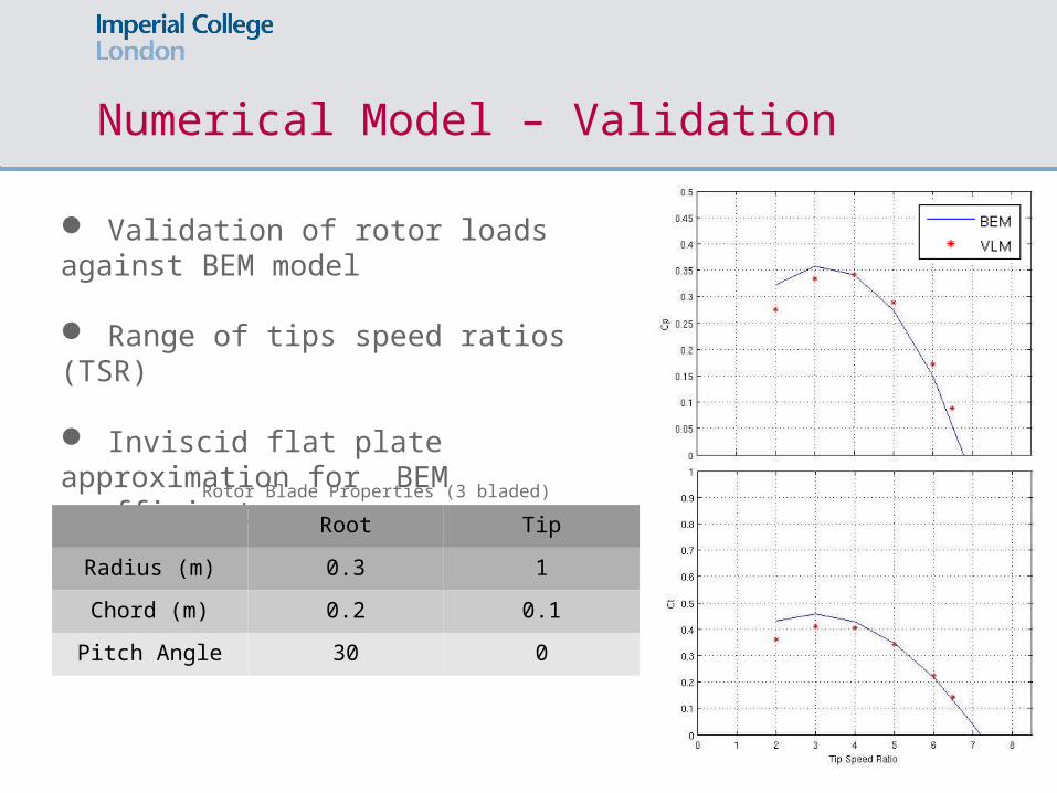
Numerical Model – Validation

Validation of rotor loads against BEM model

Range of tips speed ratios (TSR)

Inviscid flat plate approximation for BEM coefficients

Root Tip

Radius (m) 0.3 1

Chord (m) 0.2 0.1

Pitch Angle 30 0

Rotor Blade Properties (3 bladed)

Numerical Model – Demonstration

Numerical Model – Demonstration

Review

Background

Numerical Model

Results

Ongoing Work

Numerical Model – Results

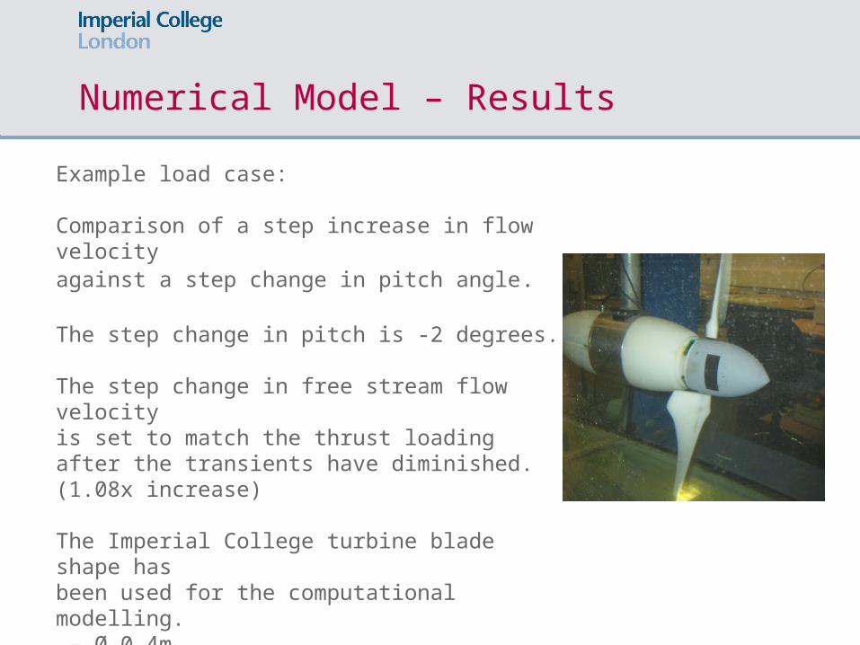
Example load case:

Comparison of a step increase in flow velocityagainst a step change in pitch angle.

The step change in pitch is -2 degrees.

The step change in free stream flow velocityis set to match the thrust loading after the transients have diminished. (1.08x increase)

The Imperial College turbine blade shape has been used for the computational modelling. – Ø 0.4m – 2 Blades – Free stream flow velocity = 1m/s – Tip speed ratio = 5

Numerical Model – Results

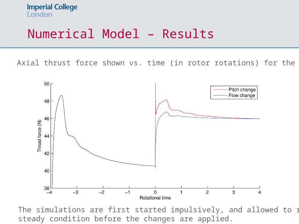
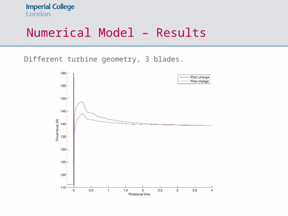
Axial thrust force shown vs. time (in rotor rotations) for the two cases:

The simulations are first started impulsively, and allowed to reach asteady condition before the changes are applied.

Numerical Model – Results

With the reverse case:

Pitch change:+2 degrees

Flow change:0.91

Numerical Model – Results

Induced velocity at the tip (μ = 0.95)

Numerical Model – Results

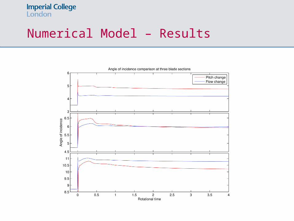
Induced velocity, thrust and angle of incidence at three radial sections:

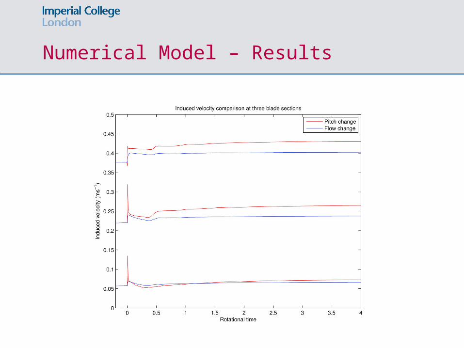
Numerical Model – Results

Numerical Model – Results

Numerical Model – Results

Numerical Model – Results

Matching induced velocity in the tip region:

Free stream velocity after change = 1.2

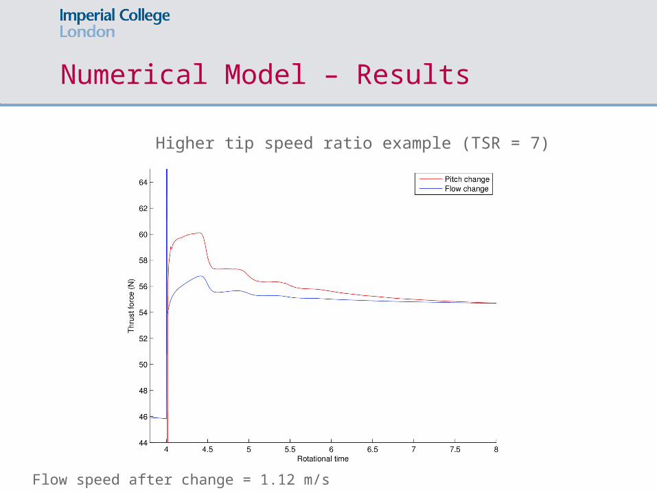
Numerical Model – Results

Higher tip speed ratio example (TSR = 7)

Flow speed after change = 1.12 m/s

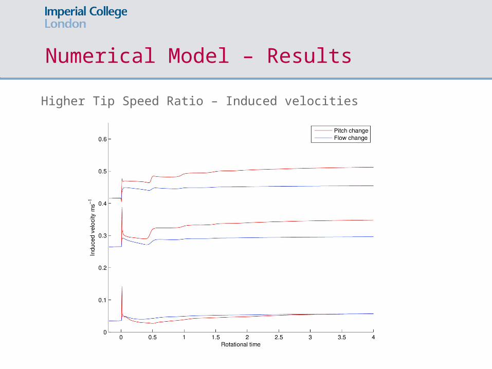
Numerical Model – Results

Higher Tip Speed Ratio – Induced velocities

Numerical Model – Results

Different turbine geometry, 3 blades.

Numerical Model – Results

Numerical work on flow oscillation:

- The vortex lattice code can be used to model sinusoidal flow oscillations

Numerical Model – Results

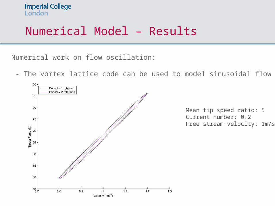
Numerical work on flow oscillation:

- The vortex lattice code can be used to model sinusoidal flow oscillations

Mean tip speed ratio: 5Current number: 0.2Free stream velocity: 1m/s

Review

Background

Numerical Model

Results

Ongoing Work

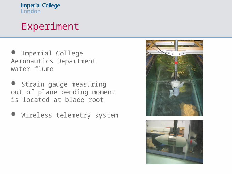
Experiment

Imperial College Aeronautics Department water flume

Strain gauge measuring out of plane bending moment is located at blade root

Wireless telemetry system

Ongoing Work

Comparison of numerical model with common engineering model – (e.g. Pitt and Peters for dynamic inflow)

Numerical improvements

Comparison of VLM with experimental data

Investigate more load cases:- wave motion

Conclusion

A vortex lattice method solver has been created to model flow unsteadiness in power generating turbines

The effect of flow unsteadiness and dynamic inflow on rotor loading has been demonstrated

Dynamic inflow has been shown to be significant for some unsteady cases.

Thanks,

Duncan McNae

Reverse Case Mirrored

Numerical Model – Results

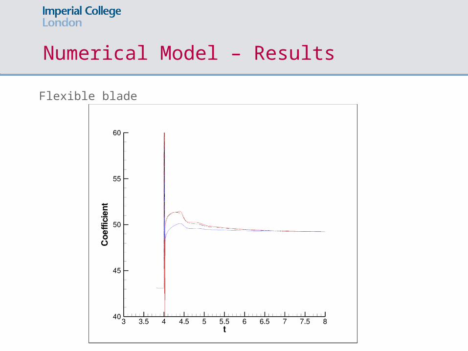
Flexible blade