Particularities of Membrane Gas Separation Under Unsteady State
Upload
evelyn-lauritoCategory
view
9.437download
14
Unsteady State Conduction
Evelyn R. LauritoLani Pestano
Ch.E. 206
Lecture Objectives
To understand the concept of unsteady state conduction
To study the case of unidirectional unsteady state conduction
To understand how to use Geankoplis Charts in solving unidirectional unsteady state conduction problems
Gurney and Lurie Charts Heisler Chart Chart for Average Temperature Chart for Semiinfinite solid
To understand how to use Numerical Methods in solving unidirectional unsteady state conduction problems
Unsteady State Conduction
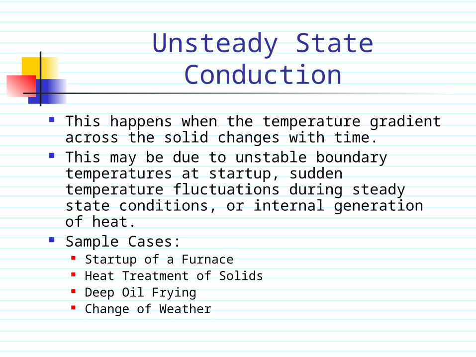
This happens when the temperature gradient across the solid changes with time.
This may be due to unstable boundary temperatures at startup, sudden temperature fluctuations during steady state conditions, or internal generation of heat.
Sample Cases: Startup of a Furnace Heat Treatment of Solids Deep Oil Frying Change of Weather
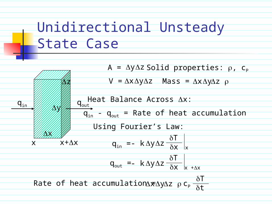
Unidirectional Unsteady State Case
x
y
z
x x+x
qin qout
A = yz
V = xyz
Solid properties: , cP
Mass = xyz
Heat Balance Across x:
qin - qout = Rate of heat accumulation
Rate of heat accumulation = xyz Tt
Using Fourier’s Law:
qin = - k yzTx x
qout = - k yzTx x +x
cP
Unidirectional Unsteady State Case
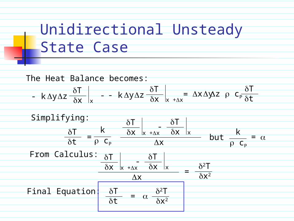
The Heat Balance becomes:
- k yzTx x
- - k yzTx x +x
= xyz cP
Tt
Simplifying:
Tt =
k cP
Tx x +x
- Tx x
x
From Calculus: Tx x +x
- Tx x
x=
2Tx2
Final Equation: Tt =
k cP
= but
2Tx2
Unidirectional Unsteady State Case
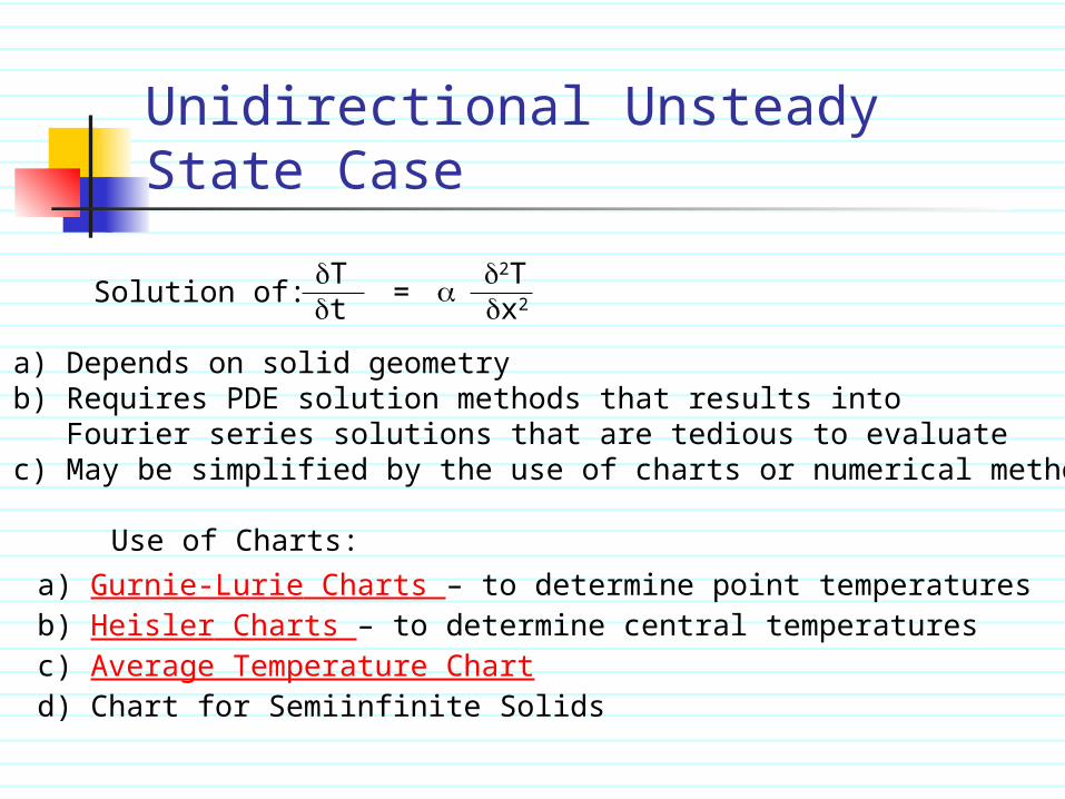
Tt =
2Tx2Solution of:
a) Depends on solid geometryb) Requires PDE solution methods that results into
Fourier series solutions that are tedious to evaluatec) May be simplified by the use of charts or numerical methods
Use of Charts:
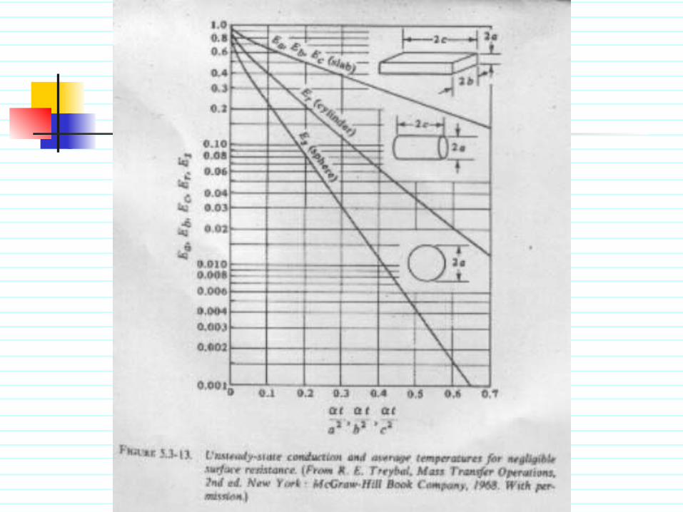
a) Gurnie-Lurie Charts – to determine point temperaturesb) Heisler Charts – to determine central temperaturesc) Average Temperature Chartd) Chart for Semiinfinite Solids

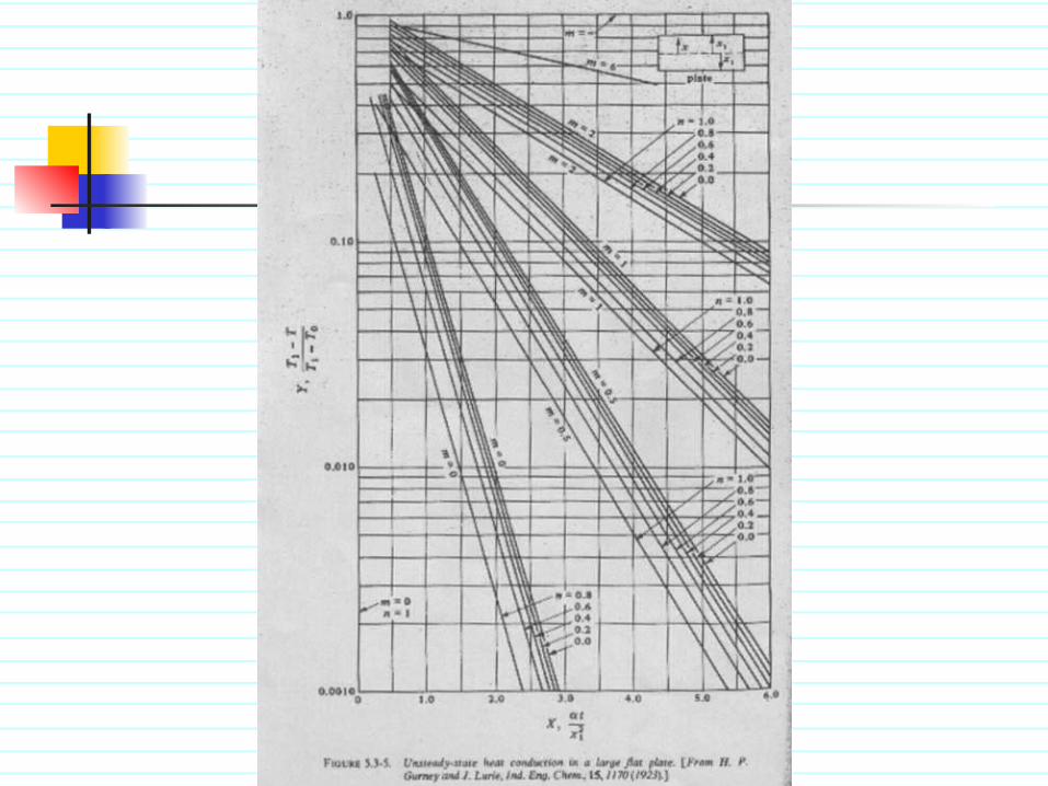
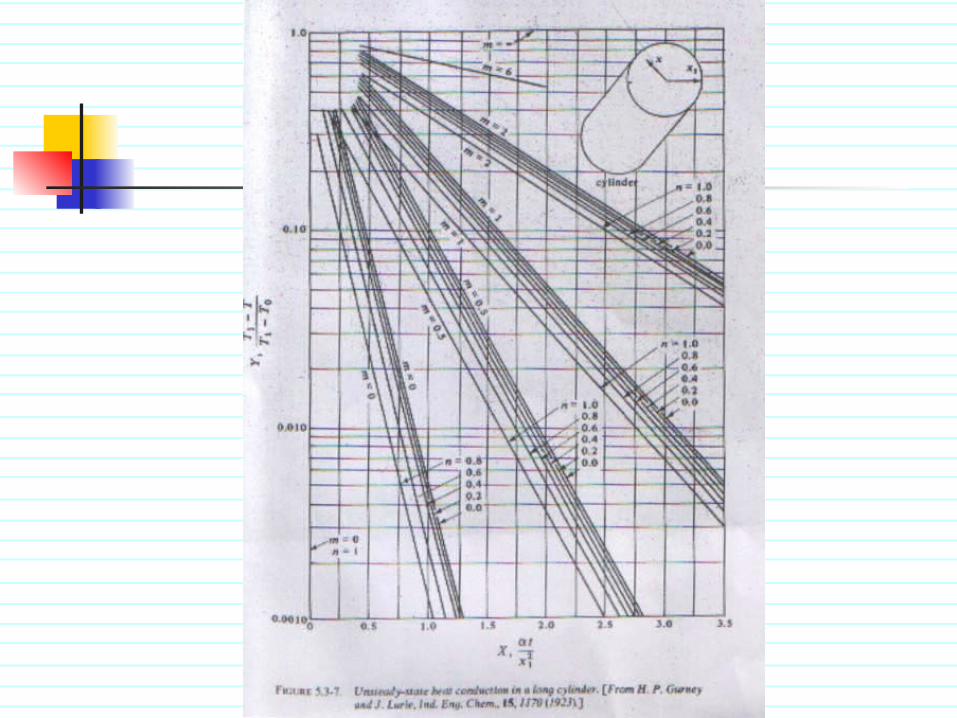
Geankoplis Charts Gurney-Lurie Charts
Fig. 5.3-5/340 for large flat plate Fig. 5.3-7/343 for long cylinder Fig. 5.3-9/345 for sphere
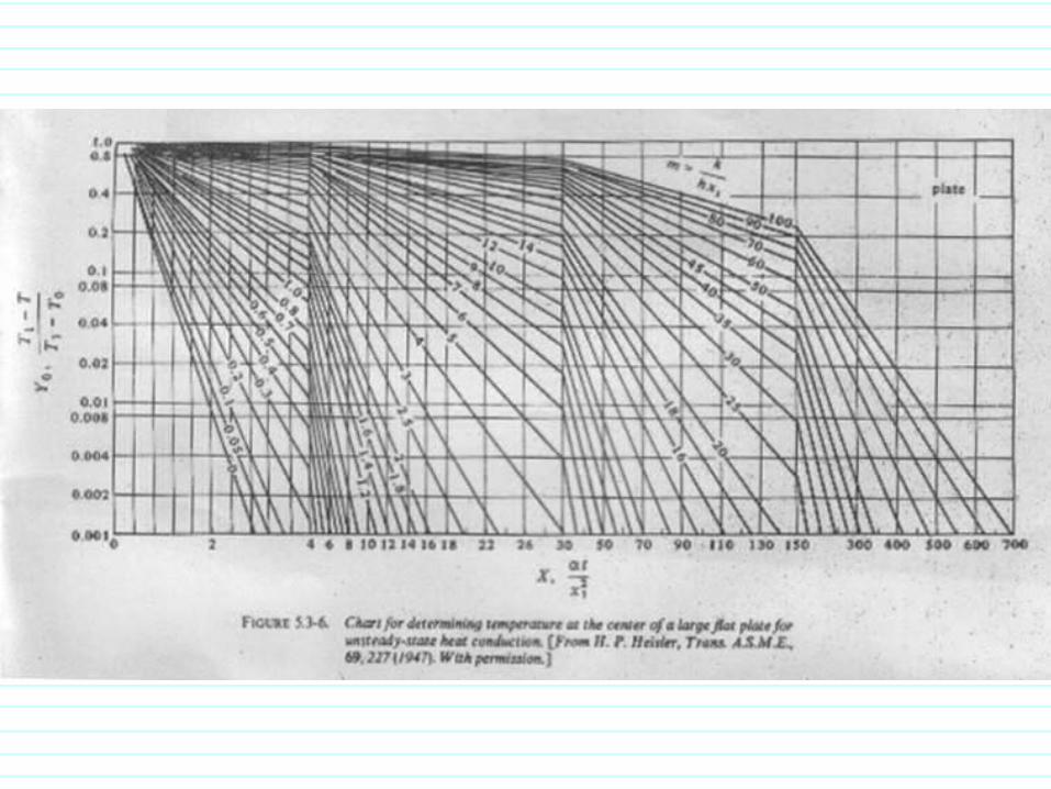
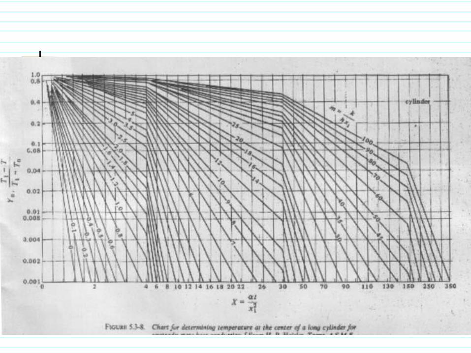
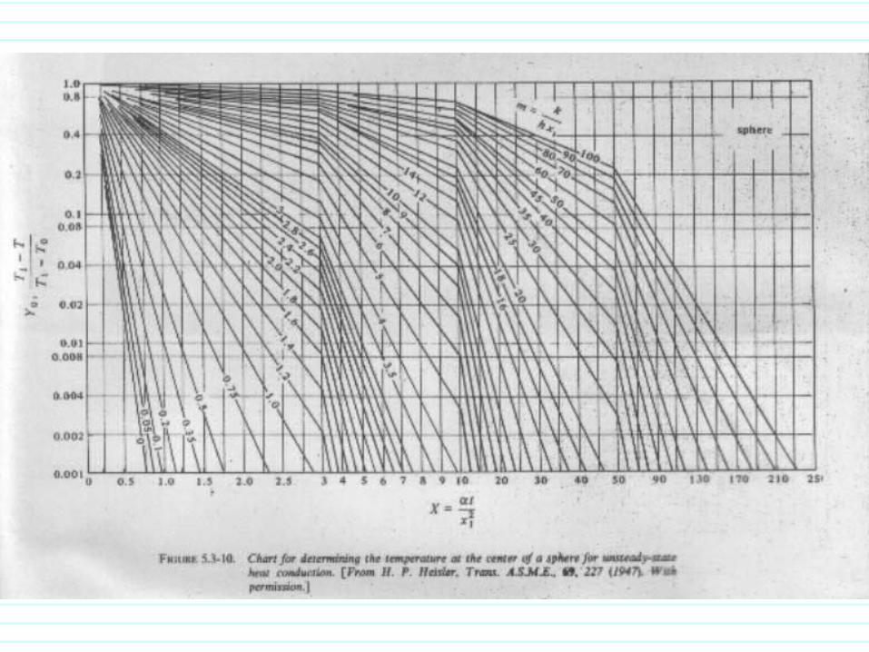
Heisler Chart Fig. 5.3-6/341 for large flat plate Fig. 5.3-8/344 for long cylinder Fig. 5.3-10/346 for sphere
Fig. 5.3-13/349 for Ave. Solid Temperature Fig. 5.3-3/337 for Semi-infinite solid

Nomenclature Gurney-Lurie and Heisler Charts:
To = temperature at t(time)= 0 (uniform) T1 = new and constant surface temperature x1 = ½ plate thickness, outer radius of cylinder or sphere = constant thermal diffusivity X = t/ x1
2 : relative time x = distance from plate center or any radius of a
cylinder or a sphere n = x/x1: relative position T = point temperature at position x and time t Y = (T1-T)/(T1-To) :unaccomplished temp. change h = convective heat transfer coefficient m = k/(hx1) : relative resistance
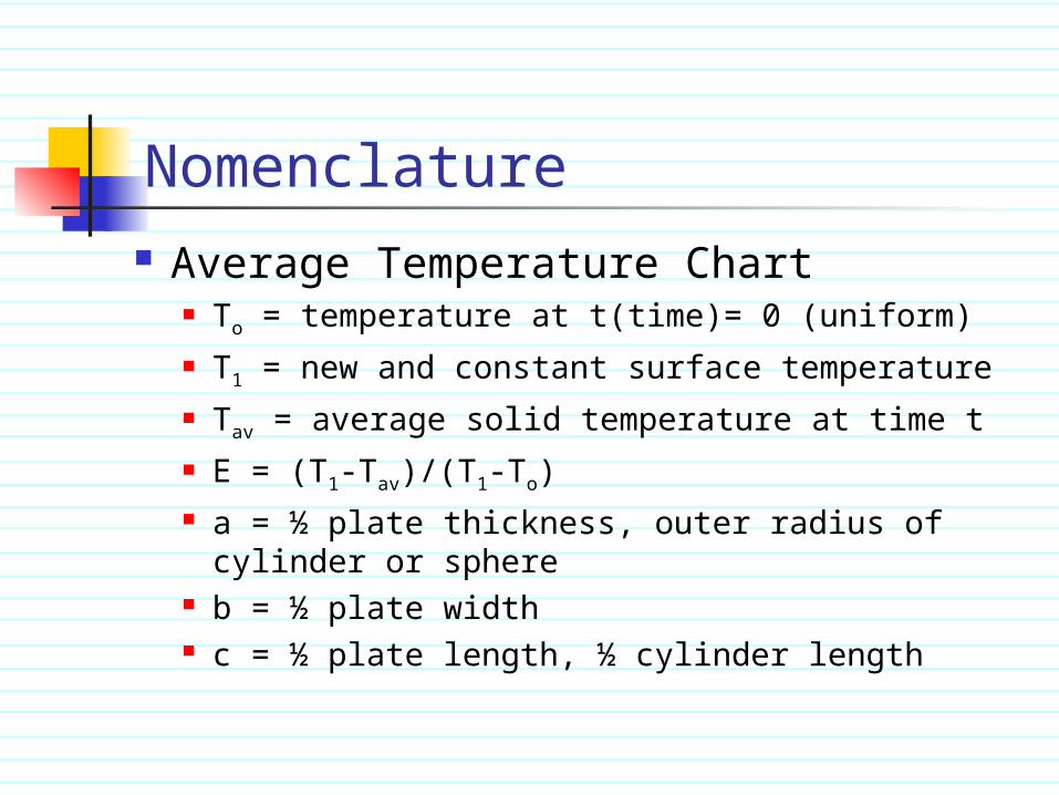
Nomenclature Average Temperature Chart
To = temperature at t(time)= 0 (uniform) T1 = new and constant surface temperature Tav = average solid temperature at time t E = (T1-Tav)/(T1-To) a = ½ plate thickness, outer radius of
cylinder or sphere b = ½ plate width c = ½ plate length, ½ cylinder length
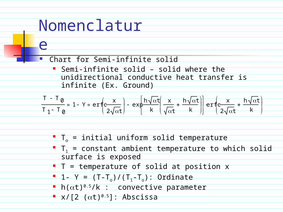
Nomenclature Chart for Semi-infinite solid
Semi-infinite solid – solid where the unidirectional conductive heat transfer is infinite (Ex. Ground)
To = initial uniform solid temperature T1 = constant ambient temperature to which solid
surface is exposed T = temperature of solid at position x 1- Y = (T-To)/(T1-To): Ordinate h(t)0.5/k : convective parameter x/[2 (t)0.5]: Abscissa
T T 0
T 1 T 01 Y erfc
x
2 t
exph tk
x
t
h tk
erfc
x
2 t
h tk
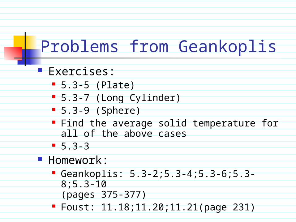
Problems from Geankoplis Exercises:
5.3-5 (Plate) 5.3-7 (Long Cylinder) 5.3-9 (Sphere) Find the average solid temperature for all of
the above cases 5.3-3
Homework: Geankoplis: 5.3-2;5.3-4;5.3-6;5.3-8;5.3-10
(pages 375-377) Foust: 11.18;11.20;11.21(page 231)
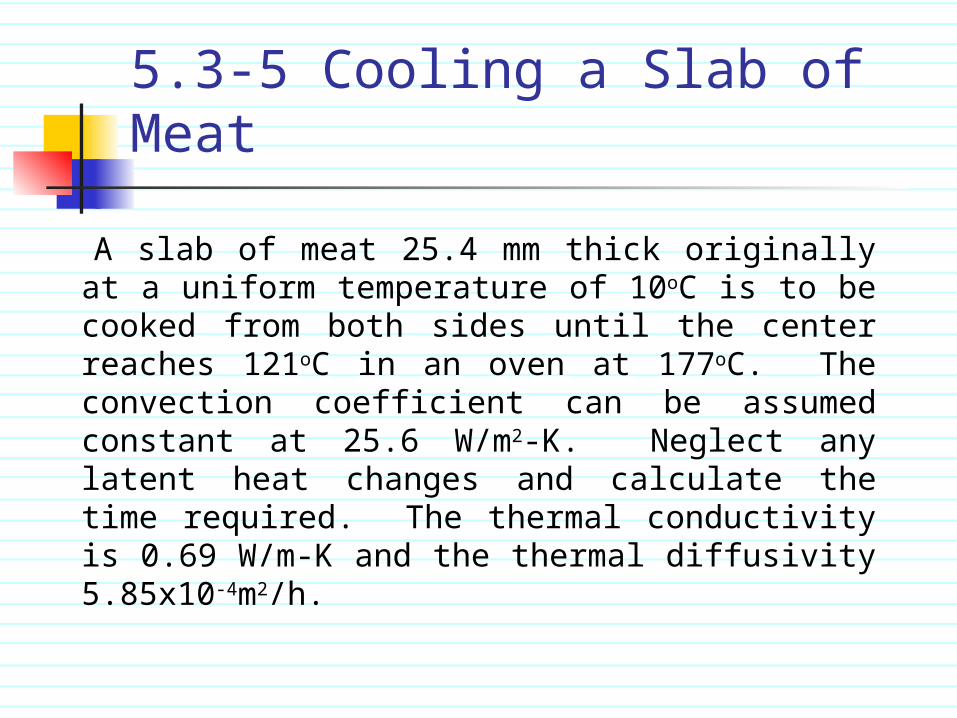
5.3-5 Cooling a Slab of Meat
A slab of meat 25.4 mm thick originally at a uniform temperature of 10oC is to be cooked from both sides until the center reaches 121oC in an oven at 177oC. The convection coefficient can be assumed constant at 25.6 W/m2-K. Neglect any latent heat changes and calculate the time required. The thermal conductivity is 0.69 W/m-K and the thermal diffusivity 5.85x10⁻⁴m2/h.

Solution for 5.3-5Given:
t= 25.4 mmTo=10oC
T=121oC (Center T) at x1
T1=177oC
h=25.6 W/m2-Kk=0.69 W/m-K=5.85x10-4m2/h
Required: t= ?
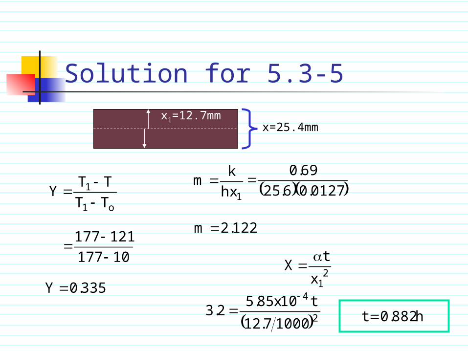
Solution for 5.3-5x1=12.7mm x=25.4m
m
x
tX
21
TT
TTY
o1
1
10177
121177
3350Y .
hx
km
1
01270625
690
..
.
1222m .
1000712
t10x85523
2
4
.
..
h8820t .

5.3-7 Cooling of a Steel Rod
A long steel rod 0.305 m in diameter is initially at a temperature of 588K. It is immersed in an oil bath maintained at 311K. The surface convective coefficient is 125 W/m2-K. Calculate the temperature at the center of the rod after 1 h. The average physical properties of the steel are k=38 W/m-K and =0.0381m2/h
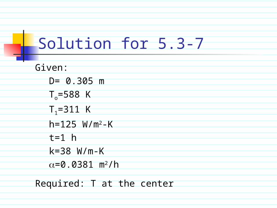
Solution for 5.3-7Given:
D= 0.305 mTo=588 K
T1=311 K
h=125 W/m2-Kt=1 hk=38 W/m-K=0.0381 m2/h
Required: T at the center
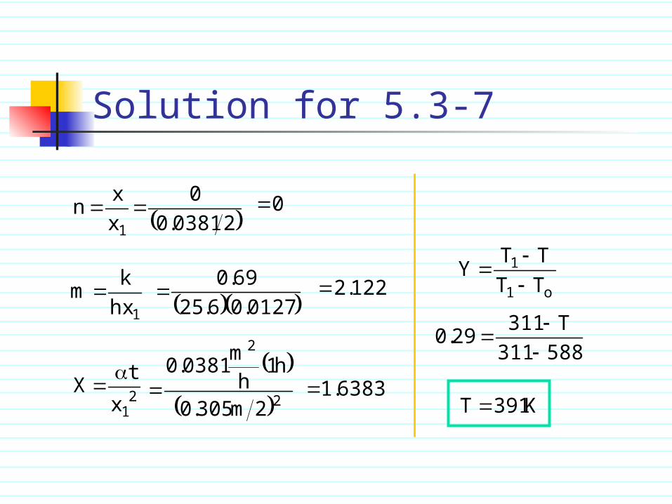
Solution for 5.3-7
x
tX
21
TT
TTY
o1
1
K391T
hx
km
1
01270625
690
..
. 1222.
2m3050
h1h
m03810
2
2
.
.
x
xn
1
203810
0
. 0
63831.
588311
T311290
.
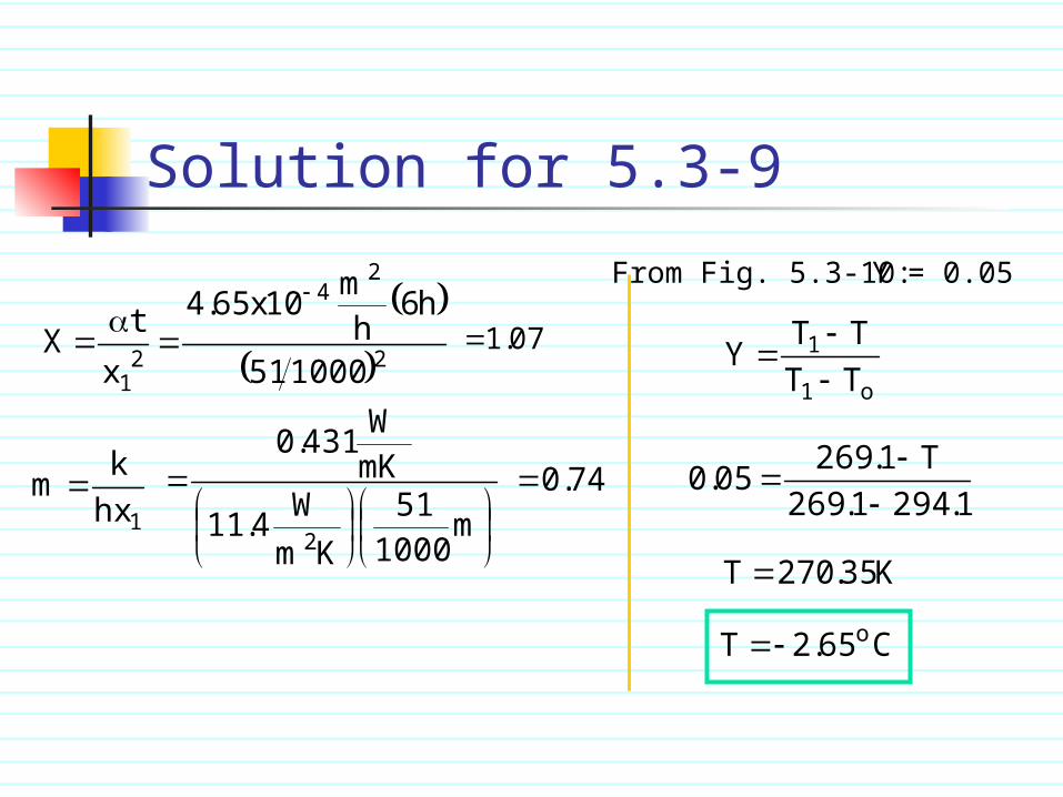
5.3-9 Temp. of Oranges on Trees During Freezing Weather
In orange-growing areas, the freezing of the oranges on the trees during cold nights is economically important. If the oranges are initially at a temperature of 21.1oC, calculate the center temperature of the orange if exposed to air at –3.9oC for 6 h. The oranges are 102 mm in diameter and the convective coefficient is estimated as 11.4W/m2-K. The thermal conductivity k is 0.431 W/m-K and =4.65x10-
4m2/h. Neglect any latent heat effects.

Solution for 5.3-9Given:
D= 102 m x=102/2=51mmTo=21.1oC=294.1K
T1=-3.9oC=269.1K
h=11.4 W/m2-Kt=6 hk=0.431 W/m-K=4.65x10-4 m2/h
Required: T at the center
Solution for 5.3-9
x
tX
21
TT
TTY
o1
1
K35270T .
hx
km
1
m
100051
Km
W411
mKW
4310
2
.
. 740.
100051
h6h
m10x654
2
24
.
071.
12941269
T1269050
..
..
From Fig. 5.3-10:Y = 0.05
C652T o.
5.3-3 Cooling a Slab of Aluminum
A large piece of aluminum that can be considered a semi-infinite solid initially has a uniform temperature of 505.4K. The surface is suddenly exposed to an environment at 338.8K with a surface convection coefficient of 455W/m2-K. Calculate the time in hours for the temperature to reach 388.8 K at a depth of 25.4 mm. The average physical properties are =0.340m2/h and k=208W/m-K.
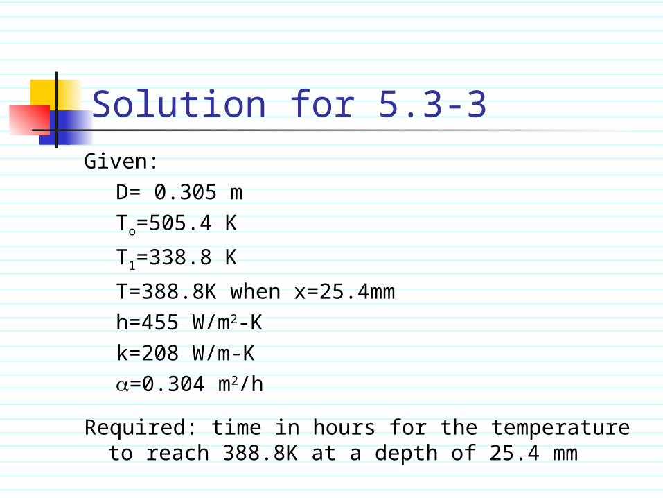
Solution for 5.3-3Given:
D= 0.305 mTo=505.4 K
T1=338.8 K
T=388.8K when x=25.4mmh=455 W/m2-Kk=208 W/m-K=0.304 m2/h
Required: time in hours for the temperature to reach 388.8K at a depth of 25.4 mm
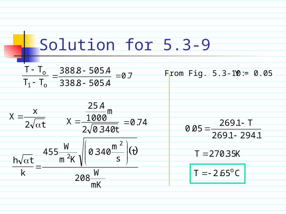
Solution for 5.3-9
t2
xX
TT
TT
o1
o
K35270T .
k
th
mKW
208
ts
m3400
Km
W455
2
2
.
740.
70.
12941269
T1269050
..
..
From Fig. 5.3-10:Y = 0.05
C652T o.
45058338
45058388
..
..
t34002
m1000
425
X.
.