Computational-Fluid-Dynamics-Based Kriging …cfdbib/repository/TR_CFD_08_38.pdf ·...

Computational-Fluid-Dynamics-Based Kriging

Optimization Tool for Aeronautical Combustion

Chambers

F. Duchaine ∗, T. Morel † and L.Y.M. Gicquel ‡

CERFACS, 42 Av. G. Coriolis, 31057 Toulouse, France

Current state-of-the-art in Computational Fluid Dynamics (CFD) provides rea-

sonable reacting flow predictions and is already used in industry to evaluate new

concepts of gas turbine engines. In parallel, optimization techniques have reached

maturity and several industrial activities benefit from enhanced search algorithms.

However, coupling a physical model with an optimization algorithm to yield a deci-

sion making tool, needs to be undertaken with care to take advantage of the current

computing power while satisfying the gas turbine industrial constraints. Among the

many delicate issues for such tools to contribute efficiently to the gas turbine indus-

try, combustion is probably the most challenging and optimization algorithms are

not easily applicable to such problems. In our study, a fully encapsulated algorithm

addresses the issue by making use of a new multi-objective optimization strategy

based on an iteratively enhanced meta-model (Kriging) coupled to a Design of Ex-

periments (DoE) method and a fully parallel three dimensional (3D) CFD solver

to model turbulent reacting flows. With this approach, the computer cost needed

for thousands of CFD computations is greatly reduced while ensuring an automatic

error reduction of the approximated response function. Preliminary assessments

of the search algorithm against simple analytical test functions prove the strategy

to be efficient and robust. Application to a 3D industrial aeronautical combustion

chamber demonstrates the approach to be feasible with currently available com-

puting power. One result of the optimization is that possible design changes can

improve performance and durability of the studied engine. With the advent of

∗Post.-Doc., CFD Combustion Team.†Researcher Engineer, Global Change Team.‡Senior Researcher, CFD Combustion Team.

1 of 43

American Institute of Aeronautics and Astronautics

massively parallel architectures, the intersection between these two advanced tech-

niques seems a logical path to yield fully automated decision making tools for the

design of gas turbine engines.

2 of 43


Nomenclature

X Set of optimization parameters

X? Global optimum parameters

f(X) Objective function of optimization parameters X

f(X) Approximation of f(X)

σf (X) Variance of the approximation f(X)

fM Merit function

% Parameter of the merit function

Φβ Criterion of spatial homogeneity of samples in a design space

ηc Combustion efficiency

θ Parameter of the combustion efficiency

Prsf Stator thermal stress criterion

T Temperature

P Pressure

V Velocity

Q Mass flow rate

ρ Flow density

Vc Volume of the primary zone

ma Air mass flow entering the primary zone

σ Porosity of multi-perforated plates

S Surface

Ppi Position of primary jets

Pdt Air flow split between the swirler and the multi-perforated plates

Pmp Air flow split between external and internal multi-perforated plates

Subscript

3 Compressor value

4 Plane 4 value

T Swirler value

MP Multi-perforation value

Superscript

a Dimensionless value

b Baseline value

3 of 43


e External value

i Internal value

ref Reference value

I. Introduction

Systematic use of optimization for gas turbine combustion chambers is usually limited due to

the substential computing power required by such applications. Furthermore, global optimization

strategy remains beyond today’s limits and well tuned, targeted search methods (based on know-

how) in a restrained design space are the only viable options. Despite these constraints, numerous

domains have seen the advent of fully automated decision-making tools to help the design of new

devices. In fluid mechanics, contributions remain quite limited because of the difficulty in obtaining

accurate flow estimates and the need for highly computer demanding algorithms. Flow predictions

in real applications are usually obtained by Computational Fluid Dynamics (CFD) which necessitate

the numerical solution of spatially and temporally dependent partial differential equations. The

resolution of this system of equations usually takes four to five hours on modern supercomputers.

That non-negligible computational effort accentuates the need for intensive computing facilities

especially if optimization is targeted. It also underlines the necessity for very efficient search

procedures such as gradient methods using adjoint CFD solvers.1 Availability of the adjoint CFD

solver partly explains why CFD based optimization is mostly developed for purely aerodynamic

problems,2,3 where the maturity of the CFD codes allows access to the adjoint solvers. Recent

applications of such optimization tools to 3D aerodynamic problems have been realized4–7 with

success.

A direct application of aerodynamic oriented techniques to fully turbulent reacting flows is not

trivial. Indeed, the extended physics implied by turbulent reacting flows involve strong couplings

between combustion, mixing and flow dynamics which make the development of CFD adjoint solvers

a difficult task. Gradient estimations can still be obtained by finite difference techniques. However,

this approach is known to be sensitive to the noise generated by the numerical solution of the system,

the grid management as well as all the various transformations introduced by the optimization

process.8 Direct deterministic search methods9 are thereof preferred. The primary reasons are their

reliability, ease of implementation, applicability to non-linear and non-differentiable problems where

they yield good results when sophisticated approaches fail.10 These methods are also easy first

4 of 43


choices before going into the development of more complex approaches. They are also available in

most optimization tools: i.e. Nimrod,11,12Dakota,13 Condor,14 OPT++,15 iSIGHT,16 Optimus.17

In the context of optimization, algorithm design is faced with two conflicting criteria. ”Ex-

ploration” indicates the capability of a method to search global interesting configurations over

the whole design space. On the contrary, ”exploitation” indicates the capability of using already

known information to rapidly converge to a local optimum. Among the deterministic approaches,

zero order models are usually limited to local searches while performing an efficient exploitation of

the available data to converge rapidly to an optimum in the neighborhood of the starting point.

Exploration remains critical if a global optimum is targeted. Stochastic processes are usually intro-

duced to extend the local search by random identification of several initial search points.18 Genetic

algorithms are the most commonly used stochastic methods.8,19–21 Finally, the coupling of efficient

gradient approaches with stochastic methods would ensure efficient local and global search.22

As pointed out initially, the most important constraint for the development of CFD based

optimization tools, is the limitation on CPU resources: the tool should provide an acceptable

response time even with CPU demanding applications while respecting industrial constraints. For

example, the N3S-Natur CFD code needs approximately four wall-clock hours to provide a flow field

estimate in a single sector helicopter combustion chamber. For that specific reason and since most

of the cited optimization methods require multiple evaluations of the objective functions, a reduced

fidelity model23 is introduced to limit the number of expensive CFD runs. The primary idea with

this approach is to model the optimization function by an estimate based on a limited number of

expensive CFD evaluations, thereby decreasing the overall CPU effort and elapsed time. With the

algorithm developed in this work and contrarily to conventional approches, the response surface

model is iteratively improved to limit the errors introduced with the estimate. The enhancement

of the database, on which the approximation is based, is obtained through automatic requests for

new CFD based evaluations which thus provide a set of considered exact values of the response

function. Note that the new method has the advantage of not requiring any CFD adjoint solver

and is directly applicable to turbulent reacting flow configurations as targeted in this work. Similar

simpler Kriging based strategies are adopted in other researches24 and prove to be quite successful

in their own areas of application.

When faced with industrial problems, engineers have to deal with multi-objective optimiza-

tion25 and the most appropriate approach consists in providing Pareto-optima to ease decision

making.26–29 For that type of optimization problems, access to the optimal solutions is of greatest

interest to the designer. However, it should not prevent from identifying the tendencies and depen-

5 of 43


dencies of the design to critical parameters which are valuable information for future developments.

Design of Experiments (DoE) is in that case mandatory to efficiently sample the design space30,31

and provide efficient analyses of the data.32 With the approach presented, that specificity is auto-

matically addressed since the fully automated decision making tool is essentially dedicated to the

improvement of the DoE. Indeed, a DoE is used to construct the estimator (Kriging) which gives

access to a local uncertainty on the estimate. This uncertainty is thus optimized by locally refining

the DoE thanks to new CFD evaluations.

The document is organized as follows. Specific issues pertaining to the tool automatization,

the code management and the optimization algorithm are detailed in sections II-A-B, II-C and III

respectively. Verifications and illustration of the impact of the relevant optimization parameters

are presented and discussed in section IV-A. Finally, an application to a 3D single sector of a real

combustion chamber (section IV-B) is analyzed to illustrate the applicability of the procedure to

an industrial case. It results from the demonstration that new design points can be proposed to

improve performance and durability of the studied engine.

II. Parameterization of CFD and optimization algorithms

Optimization requires the definition of control parameters determining the search space over

which the studied configuration has to be improved. In the aeronautical context, the set of design

parameters is very large and cannot be used as a whole. For simplicity, only geometrical and inflow

conditions are chosen as possible optimization criteria. That is to say that a given combustion

chamber is improved acting on a limited set of parameters and not totally designed from scratch.

The user defines cost functions on the search space to assess the quality of a given design in that

space. All the state variables and the functions are evaluated from CFD runs. In practice, the

steps needed for the preparation of a CFD run are linked to the mathematical formulation of a

fluid mechanics problem: defining the flow domain, enforcing the initial and boundary conditions

and evaluating the solution for the given set of model equations. A CFD run is hence decomposed

in three phases:

• Pre-processing: including automatic mesh generation when shape optimization is concerned,

initialization of the physical fields and determination of the boundary conditions,

• CFD computation: solution of the turbulent reacting model equations,

• Post-processing: automatic analysis of the CFD prediction for evaluation and optimization.

6 of 43


The integration of CFD in an automatic strategy for an optimization tool requires to encapsulate

these three steps in an efficient and robust package with limited user inputs. Some elements

concerning the pre- and post-processing phases are given below. Particularities related to the

optimization itself are detailed in section III.

The turbulent reacting CFD code used to provide the flow prediction of the aeronautical com-

bustion chambers is N3S-Natur. It is based on a Reynolds Average Navier-Stokes (RANS) approach

and determines the mean stationary flow features for two-phase turbulent reacting flows in com-

plex geometries using tetrahedral grids. Details on the turbulent closures, the turbulent combustion

models and the two-phase flow solver are available in Ref.33 For our work, the following options are

used: an implicit solver based on a Gauss-Siedel inversion (first order in time with local time step-

ping) with a MUSCL second order spatial scheme making use of Van Leer limiter. The turbulence

model is the standard k − ε closure. The turbulent combustion closure is the CLE model.34,35 If

dealing with two-phase reacting flows, as encountered for the real burner application, a Lagrangian

model is activated and coupled to the CFD solver. Convergence of the CFD solver is based on flux

balances for mass, total enthalpy and kinetic energy. The CFD solution is thus obtained when all

flux balance estimates reach values strictly below 1% of the previous estimate. That stop criterion

is used for all of our computations unless specified otherwise. Evaluations of the impact on the

optimization predictions of that specific criterion was assessed and found to be weak as long as all

balances were below that critical value. Validation and verification of the CFD code can be found

in Refs.34,35

A. CFD Pre-processing

The initial combustion chamber design being provided, the computational domain description is

assumed to be available through the Computed Aided Design (CAD) parameterization.36–40 There-

fore, automation of the initial and subsequent computational meshes is not addressed in detail. Only

mesh quality is discussed since it is known to be a critical point when solving partial differential

equations using numerical methods.41 Indeed, great care must be taken to generate a computational

grid which ensures meaningful CFD predictions. In the context of geometrical optimization, which

involves transformations of an initial computational domain, two methods have been implemented

and tested. The first one, generally named moving mesh technique,42–45 consists in updating an

existing discretization to meet the new set of geometrical parameters. It simply means adjusting

the initial grid node positions to fit the new design. Although this method is rather simple to

implement, it is limited to small control parameter variations to guarantee acceptable mesh quali-

7 of 43


ties. The second technique aims at fully or partially regenerating a new grid for the new given set

of geometrical parameters. Once the geometrical parameterization and regeneration processes are

well controlled, this method offers numerous possibilities to produce good quality grids even for

complex configurations.46–48 For the present work, the full regeneration technique is preferred.

The initialization of the physical fields for a given computational domain is also of practical im-

portance. It has a great influence on the time taken by the CFD computation to reach convergence

(the only time when the prediction is meaningful and can be post-processed). For our approach,

interpolations based on first order spatial Taylor developments are used to project the baseline

fields on the new grids. Finally and for most problems, adjustment of the boundary conditions to

meet the specified control parameters is trivial.

B. CFD Post-processing

Post-processing steps are of two types in our optimization process. First, it is used to verify the

flow prediction provided by the CFD code: i.e. to discriminate unphysical solutions potentially

obtained with the CFD solver. These verifications are performed through the evaluation of several

mass and energy balances as well as analyses of extreme physical quantities. Second, once verified,

the CFD results are processed to evaluate cost-functions for the given values of the control param-

eters. For the specific problems addressed here, these objective function values are computed using

local, planar and/or volumetric diagnostics which are easily obtained by manipulation of the CFD

prediction and its computational grid.

C. Management of the integrated optimization platform

The fully encapsulated tool is composed of two main components: a) the optimizer and b) the CFD

sequences which seek a prediction/approximation of the turbulent reacting flow. Both components

are themselves divided in fundamental sequences corresponding to mathematical or geometrical

operations and which often rely on specific computer codes. The first consequence of that multi-

code environment is the need for an efficient management technique of all the components (some

of which are parallelized) as well as the execution of some of the components themselves in paral-

lel. At the same level of importance, one notes the need for an efficient management of the data

transfers between elements to ensure a robust and flexible tool. The use of a coupling device is

retained to satisfy at best all of these prerequisites. The dynamic parallel code coupler PALM49

offers such capabilities and the optimization platform which results from the present developments

is based on this device. Within PALM, the application is decomposed in independent units al-

8 of 43


lowing non-hierarchical coding: the different units can be launched competitively or successively

according to the general algorithm and units exchange data by parallel MPI protocols, Fig. 1. The

optimization application, called MIPTO for Management of an Integrated Platform for auTomatic

Optimization, directly inherits from these capabilities and takes advantage of High Performance

Computing (HPC) through the use of parallel units (i.e. parallel CFD codes) and simultaneous

tasks (i.e. simultaneous CFD evaluations) management. The efficient CPU management with a

device such as PALM also justifies the optimization methods as detailed below. Note that no disk

access is necessary as dynamic addressing is fully managed for data transfer between codes/units. If

re-meshing techniques necessitate a commercial software (i.e. GAMBIT50 in the coming example),

MIPTO is able to send requests to check for license availability. That software may be accessed

on a distant server if not available where the application is operating. Details about the developed

and implemented methods in MIPTO can be founded in Ref.51

III. The optimization process

The optimization methodology is constructed to:

• Provide relationships between control variables and objective functions (mean tendencies,

relative importance of optimization parameters),

• Inform about local and global optima for each objective function,

• Detect the conflicts between cost functions by identifying Pareto Fronts.52

The core of the procedure is based on the construction of an approximate model or Meta-Model23

(MM) for each objective function. The principal advantage of such MMs is to limit the number of

computations involving full 3D CFD evaluations that are known to be very computer intensive and

time consuming. The sample databases (DBs) used to compute the MMs are initially constructed

from a finite set of CFD runs chosen by a Latin Hypercube Sampling (LHS) algorithm.53 The DBs

are then iteratively enhanced by adding new samples evaluated by new CFD computations. These

evaluations are chosen by parametric operators that give more or less importance to exploration

and exploitation. These new samples are chosen based on the uncertainty information contained

in the MMs and aim at reducing the uncertainty of the next MMs.

9 of 43


A. The Kriging estimator as meta-models

In the context of optimization, a wide variety of surrogate models are used in the literature to

approximate expensive evaluations of fitness functions. The most prominent methods among all

approaches are polynomial models,54 artificial neural networks,55 radial basis function networks56

and Gaussian processes (GPs).57 Among these empirical models, GPs appear to be the most promis-

ing for fitness function approximations. Indeed, GPs combine the following decisive properties and

were successively applied for combustion problems:24,58

• The implementation of GPs is independent of the number of decision variables,

• GPs can accurately approximate arbitrary functions including multi-modalities and disconti-

nuities,

• GPs contain meaningful Hyper-Parameters (HPs) that can be obtained theoretically with an

optimization procedure,

• GPs yield an uncertainty measure of the predicted value in the form of a standard deviation.

Two MMs are available in the developed tool. The first one draws inspiration from ordinary

Kriging.59 The second one aims at enhancing the behavior of the estimator when faced with noisy

functions or badly sampled DBs.60 Both MMs learn their specific HPs according to the current

DBs and yield an estimator f(X) of the true function f(X) as well as the standard deviation σf (X)

of the predictor for the design point X.

B. The meta-models enhancement operators

For each iteration of the method, the enhancement of the DBs are based on two operators:

• For each objective i, a search of local optima is performed for the merit function f iM defined

by

f iM (X) = fi(X) + % σfi(X), (1)

where % is a negative user defined parameter. The value of this parameter controls the conflict

between exploration and exploitation. When % tends to 0, the exploitation is fostered. As %

decreases, more attention is given to exploration. The local optima are obtained through the

use of a multi-start strategy51 of a gradient algorithm,61

10 of 43


• The second operator acts in the case of multi-objective studies. It selects the points that

belong to the Pareto Front, obtained from the MMs with the genetic algorithm NSGA-

II,62,63 and which have the highest values of σfi(X). The operator then aims at improving

the precision of the predicted Pareto Front.

The two enhancement operators propose a set of new sample points to be evaluated using the

CFD solver. In order to optimize the use of computational resources (if the number of new samples

is not proportional to the number of simultaneous evaluations), a third party can add other samples

based on cross-over genetic type operations.64 It is important to underline that for certain sets

of control parameters, the CFD solver may not find acceptable solutions. For these points and to

avoid penalization of the merit function, the value of σfi(X) at these locations is suppressed if no

information about the objective function is provided (failed CFD).65,66

The global algorithm is presented in Fig. 2. The initial DBs (depicted by the item ”Observa-

tions” in the figure) is obtained by a DoE method. Optimal (in the sense of orthogonality and

dispersion67,68) LHS is generally used for this initialization phase. The stopping criteria for that

sequence are the total number of CFD evaluations, the number of new samples obtained by the

operators or the overall precision of the MMs. The two steps referred to as ”Observations and New

Observations” in Fig. 2 consist in evaluating independent sets of design parameters. Consequently

and depending on the available computing resources, the different evaluations can be done simul-

taneously. This feature aims at reducing the overall response time of the method while benefiting

from HPC.

IV. Algorithm verification and application to a real combustion chamber

A. Methodology verification and assessment

In order to verify the behavior of the implemented optimization method, a simple analytical cost

function for a single optimization parameter is considered. For this test and to mimic non-converged

or failed CFD computations, the design space contains a Non-Definition Zone (NDZ) where the

evaluation of the control parameter is not possible, Eq. (2),

f(X) = f(x) = −0.01(200− (x2 + 5.5x− 11)2 − (x2 + x− 7)2

)−[2.5 exp

(−(x− 1.5)2

)+ 1.3 exp

(−(x+ 4)2

)](2)

with x ∈ [−5,−0.5] ∪ [1, 5].

11 of 43


The convergence criterion for which the estimator is considered to be a good representation of the

target response function, is set to be the L2 norm of the difference between the analytical target

and its estimate. Convergence is in this case set to be below 1% and is kept as such for all of

the tests presented in this section. The convergence history of the algorithm is presented in Fig. 3

after the initialization and for the 5 subsequent iterations corresponding to the enrichment of the

DBs. With the chosen input parameter, % = −10, the merit function converges to the estimator in

only 4 iterations. The treatment of the NDZ does not disturb the method which yields final DBs

composed of samples that cover the decision space with more concentrations at local and global

optima.

As already mentioned, the choice of % has a great impact on the results provided by the method.

In order to analyze more precisely this impact, we consider the analytical multi-modal objective

function presented in Fig. 4, and given in Eq. (3),

f(X) = f(x, y) = − 0.1(x+ 4)2

− 3(1− x)2exp(−x2 − (y + 1)2

)+ exp

(−(x+ 1)2 − y2

3

)+ 10

(x5− x3 − y5

)exp

(−x2 − y2

)(3)

with X ∈ [−2, 2]× [−2.5, 2.5].

The experiment aims at observing the convergence rate towards the global optimum (denoted

by X? in Fig. 4) along with the evolution of the spatial homogeneity of the samples probed in the

design space. The last quantity is evidenced by Φβ:68

Φβ(DB) =

∑Xi∈DB

∑Xj∈DBXj 6=Xi

d(Xi, Xj)−β

1/β

(4)

where d(Xi, Xj) is a distance measure between Xi and Xj over the design space.

The precision of the MM which represents the analytical function is also gauged through the

parameter RMSE (Root Mean Square Error69) evaluated with an external test database DBT

composed of 50 samples:

RMSE =

1size(DBT )

∑X∈DBT

(f(X)− f(X))2

1/2

(5)

The accuracy of the response surface provided by the MM is assessed in Fig. 5a at each iteration

and by comparing Xmin, the set of optimization parameters that lead to the minimum objective

12 of 43


function value from the current DBs, withX?. The behavior shows convergence of the method to the

global optimum X? in the design space and in the objective function space, Fig. 5b. Clearly small

|%| values yield faster convergence of the method toward X? (emphasis on the exploitation concept).

The drawback of a fast convergence to X? is illustrated in Fig. 6. For small values of |%|, the linear

increase of Φβ goes along with a size increase of the current DBs and a homogeneous enhancement

of the DBs in the design space. As expected, large values of |%| lead to a homogeneous exploration

of the research space. On the contrary, small values tend to a fast decrease of the exploration

performances. The case % = −4 shows the typical behavior of the method: at the early stage of the

enhancement, σfi(X) is rather large when compared to fi(X). It produces a homogeneous sampling

of the search space. At latter stages, σfi(X) decreases (the predictor becomes better throughout

the design space) and the merit function converges to the predictor. The enhancement essentially

focuses on new samples located around local optima which degrade the overall homogeneity of the

sample distribution (drastic increase of Φβ).

Based on the previous set of tests, homogeneity in the search space has a direct consequence on

the precision of the MM in the design space: if there are too many samples in a reduced region of

the design space, the RMSE quality measure is degraded (RMSE tends to 1). For multi-objective

optimization processes homogeneity is preferred and % is set to a fixed value equal to −10 in the

following example.

B. Application to a real combustion chamber

1. Description of the target configuration

In this section, an application of MIPTO is presented for a TURBOMECA combustion chamber,

Fig. 7. The supplied CFD computational domain corresponds to one single sector of the full

annular flame tube. Details about the boundary conditions (location and type) as initially supplied

are presented in Fig. 8a. The meshes used for this application are unstructured and contain a mean

of 210, 000 nodes and 1, 130, 000 tetrahedral cells. The planes used to analyze the CFD predictions

as well as illustrations of the turbulent reacting flow within the chamber are presented in Fig. 8b.

Note that Plane 4 coincides here with the location of the distributor, which is a critical element

of the engine. Indeed the distributor is subject to large thermal stresses due to the temporal and

azimuthal temperature variations induced by combustion taking place in the primary zone of the

combustion chamber (region delimited by the primary jets as well as the swirled injector). One

aim of the current application is to reduce that thermal stress, hence improving the design of the

13 of 43


given chamber for a given operating point.

2. Presentation of the baseline configuration

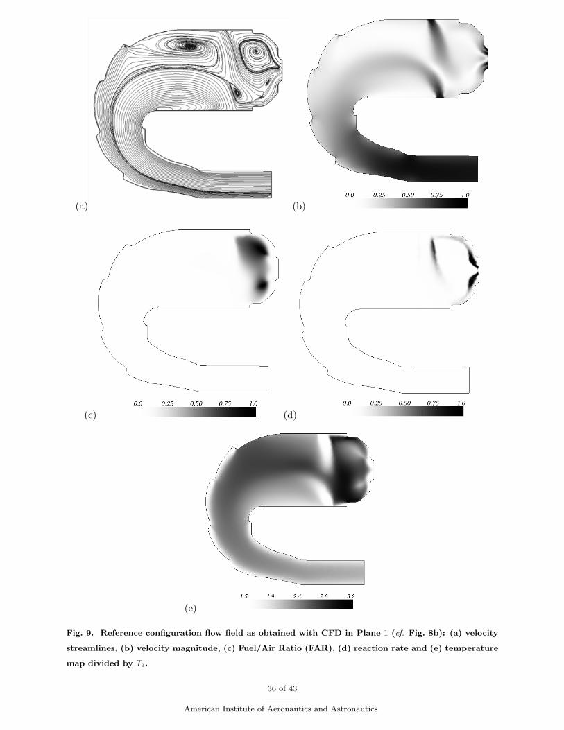
Figure 9 presents the dimensionless aerodynamic and combustion fields of the reference design.

Most of the aerodynamic activity concentrates in the primary zone of the combustion chamber.

In this region, a large re-circulation zone located after the air injector characterizes the flow. The

external primary jets bring air within the primary zone to ease combustion. The effect of the

internal jets on that part of the chamber is not so clear. Flow streamlines in Plane 1 of the

chamber show an important re-circulation zone located after the external primary jets. Note that

the re-circulating gases of the primary zone lead to fast evaporation and mixing of the liquid fuel

injected through the swirler. Combustion, visualized through the reaction rate (Fig. 9d), takes place

in the vicinity of the swirler. Fuel that is not burned in the primary zone is consumed near air

admission orifices, mostly in the neighborhood of the external primary jets. Finally, temperature

maps (non-dimensionalized by the fresh air temperature, T3) in Planes 1, Fig. 9e and Plane 2,

Fig. 10a, underline the trajectories of hot gases when leaving the primary zones.

3. Definition of the optimization problem

The considered optimization process deals with two conflicting objectives. The first one consists

of maximizing the combustion efficiency, ηc. Following Lefebvre,70 combustion efficiency for the

studied system can be expressed in term of a parameter denoted by θ and defined by:

ηc = f(θ) = f

(Pn3 Vc exp(T3/Tref)

ma

), (6)

where P3 and T3 are the pressure and the temperature of the air supplied by the compressor, ma is

the air mass flow entering the primary zone of the flame tube and Vc is its volume. The maximization

of Vc (or the minimization of the inverse of θ) leads to a maximization of the combustion efficiency.

The second objective deals with the thermal stress imposed by the hot gases impacting the

distributor, Fig. 11. A relevant measure of this stress is the profile factor at the stator location,70

Prsf , given by:

Prsf =max(T4(r))− T4

T4 − T3, (7)

where T4 is the mean exit chamber temperature, and max(T4(r)) is the maximum value of the

exit radial temperature illustrated in Fig. 11. Note that minimizing the profile factor increases

life-expectancy of the stator and the engine.

The control parameters used to minimize the objective functions (Prsf , θ−1) are of two kinds:

14 of 43


1. Geometric: the relative distance from the swirler location to the external and internal jets,

noted Ppi. Note that the axial distance which separates the external and internal jets is kept

constant.

2. Flow conditions: the total air mass flow is kept constant. Only the air flow split between

the internal, external multi-perforated plates and the swirler are changed (i.e.: Pmp, Pdt

respectively).

Figure 12 illustrates the optimization parameters. In the following, the superscript b corresponds

to the baseline configuration. In order to keep a constant total air mass flow rate entering the

flame tube, which ensures the reference operating point, constraints need to be defined on the

optimization problem. For our test, the total amount of air flowing through the multi-perforated

plates, QMP , and the swirler, QT , are adjusted to satisfy

QT = QbT Pdt, (8)

QMP = QbMP +QbT (1− Pdt), (9)

QiMP = Pmp

((1− Pdt)QbT +QbMP

), (10)

QeMP = (1− Pmp)(

(1− Pdt)QbT +QbMP

). (11)

Variations at the swirler inflow are imposed using scale similarity (proportionality) on the velocity

profiles specified at the swirler inlet boundary condition of the CFD run. Similarly, multi-perforated

inflow conditions necessitate the specification of a velocity, V , proportional to the plate’s porosity,

σ, its surface area, S and the local flow density ρ:

Q = ρ S V σ, (12)

σi =QiMP (Pdt, Ppi)

Si(Ppi)×(

Siσi

QiP iMP

)b, (13)

σe =QeMP (Pdt, Ppi)

Se(Ppi)×(

Seσe

QeP eMP

)b. (14)

In the above expressions, the superscripts i and e respectively denote the internal and external

surfaces. The quantity in parenthesis with the b superscript refers to a ratio evaluated for the

original design.

The optimization problem then looks for the optimal choices of

min

Prsf

θ−1

with

Ppi ∈ [0, Pmax

pi ],

Pdt ∈ [Pmindt , 1],

Pmp ∈ [Pminmp , P

maxmp ]

. (15)

15 of 43


4. Results of the optimization process

For the problem considered, one CFD evaluation for a given set of control parameters requires

approximately 168 CPU-hours which corresponds to 6 wall-clock hours or elapsed time if using 28

processors of a IBM JS1 power 5 1.5 GHz processors. The enhancement of the DBs is limited to

100 CFD computations (714 CPU-days on 28 processors = 25.5 days) and the initialization of the

DBs is set to provide 30 samples (210 CPU-days on 28 processors = 7.5 days). From the 100 CFD

runs, the algorithm discards 14% of the predictions (unphysical results) to construct the MMs. For

confidentiality reasons, the presentation of the results uses dimensionless quantities:

(Prsf (P ))a =Prsf (P )− (Prsf )b

(Prsf )b, (16)

(θ−1(P ))a =θ−1(P )− (θ−1)b

(θ−1)b. (17)

This normalization is to be interpreted with respect to the performance of the reference design and

negative values correspond to improved criteria while positive values indicate degradation. Note

also that both objective functions depend on P = (Pmp, Pdt, Ppi).

The analysis of the data provided by the enhancement process is presented in two steps. The

first step, inspired from sensitivity analyses,71 aims at better understanding relationships between

control parameters and objective functions. The second step deals with the actual search for

interesting new configurations after going though the optimization process.

When the number of control parameters or objective functions is quite large, sensitivity mea-

sures72,73 can guide the designer in distinguishing which parameters are the most important. For

our application, one can directly analyze the objective function responses through scatter plots,

Figs. 13 & 14. The combustion efficiency parameter θ−1 is mostly dependent on the position of

primary jets, Ppi, and to a lesser extent on the air flow split parameter, Pdt. These behaviors are

explained in light of the mathematical expression of θ−1 where Vc depends on Ppi and ma on Pdt:

θ−1 =ma(Pdt)

Pn3 Vc(Ppi) exp(T3/Tref). (18)

The objective Prsf depends on Ppi and Pdt. The role played by the mass flow passing through the

external and internal multi-perforated plates to feed the dilution process is not detectable by Prsf .

The dependency of Prsf along the design space is not as trivial as for θ−1. Focusing on the Ppi

parameter, moving the primary jets downstream leads to an increased volume of the primary zone,

which contributes to a more complete combustion. The major drawback is a shortened dilution

length and poorer mixing of the hot products by fresh gases. Hence, the Prsf criterion is degraded.

16 of 43


Looking at the effect of Pdt, one notes that below a critical value, the excess of fuel in the primary

zone is consumed thanks to the air provided by the primary jets. Mixing and dilution of hot gases

by these jets is not efficient any more and the small amount of cold air to be injected by the multi-

perforated plates is insufficient. Once again, the Prsf criterion is degraded. Beyond the critical

value of Pdt, combustion in the primary zone is more and more complete and the primary jets play

their intended role by properly mixing the hot gases: i.e. Prsf is improved.

Figure 15 presents the results of the optimization in the objective function space. The Feasible

Domain (FD) and the Pareto Front have been determined from the MMs constructed from DBs

containing 88 CFD evaluations. Based on the position of the FD in the objective function space, the

optimization process allows for potential improvement of the combustion efficiency and degradation

of the thermal criterion at the distributor location (Plane 4). Two separate zones are highlighted

on the Pareto Front. In the first one, noted Z1, it is possible to drastically improve the combustion

efficiency without degrading too much Prsf : (θ−1, P rsf ) ∈ [−0.35; 0]× [−0.1; 0.1]. On the contrary,

in the second region, noted Z2, small improvements of θ−1 lead to large degradation of Prsf :

(θ−1, P rsf ) ∈ [−0.5;−0.4]× [0.15; 0.45]. Figure 15 also underlines the fact that in the second region

of the Pareto Front, a large density of samples locates near the Pareto Front. The method has found

new interesting compromises during the last iteration and the new approximation of the Pareto

Front has not yet been explored by the enhancement operators. This also highlights the fact that

the method has not yet converged to the true Pareto Front of the multi-objective problem. However,

a compromise between computational time and convergence properties of the results needs to be

set for practical applications. Despite the mentioned shortcoming, two new design points detailed

in Table 1 seem interesting in the context of the optimization process. These potential new designs

are analyzed below, Figs. 16 to 18. The baseline configuration is presented in Figs. 9 & 10 for

comparisons.

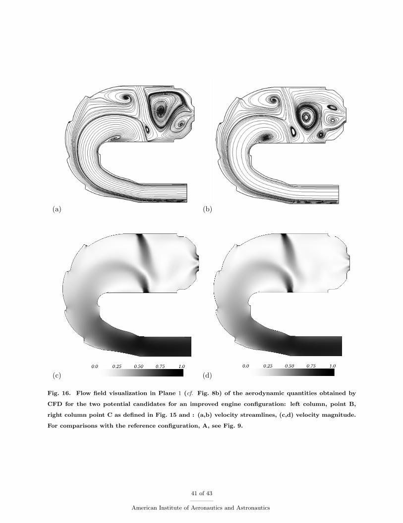
The first compromise is located along the Pareto Front, between the two identified zones of

the response function space. The second design corresponds to an improved combustion efficiency

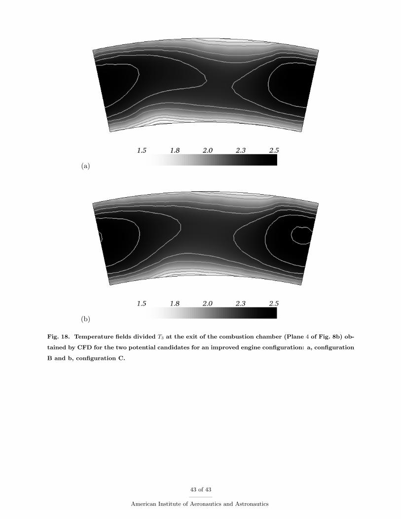
and a degraded Prsf when compared to the previous point. Figure 16 illustrates the main flow

topology differences between the two designs, while Fig. 17 concentrates on the fuel repartition

and temperature distributions, and Fig. 18 shows the exit temperature maps. As underlined and

identified in practice when defining a new combustion chamber,70 the flow topology is greatly

influenced by the position of the primary and dilution jets. When these jets are moved downstream

(away from the swirler), more and more complex flow structures coexist in the primary zone. A

second consequence of the primary jet adjustment is the reduction in intensity of the re-circulation

17 of 43


zone positioned behind the external jets and which is responsible for a large part in the mixing of

the hot products with fresh gases. The reduction in size of that flow structure goes in hand with

the intensification of a second re-circulation zone positioned behind the internal jets and which

has a limited impact on mixing. Finally, and as expected with the changes in the primary and

dilution zones inferred by the set of parameters, the new designs yield different exit temperature

fields, Fig. 18. For the retained cases, spatial heterogeneity of the exit temperature fields is clearly

observed when compared to the reference case, the original design being the optimum.

Based on the previous set of results, several rules of design can be inferred to efficiently obtain a

combustion chamber that is optimal in term of combustion efficiency and exit temperature profile.

Although necessary to shield the chamber walls from the hot product of combustion, the multi-

perforated plates do not influence the exit temperature profile. The leading parameters are for this

specific objective, the jet position and the flow rate of fresh air that is available for injection at this

location. The outer jet also plays a critical role for combustion. If not penetrating the primary

zone, fuel is burned in the mixing region of the chamber (outside the primary zone) thereby ruining

the exit temperature profile. Combustion efficiency essentially depends on the primary zone volume

or equivalently the outer jet position. The aim of the designer is thus to have the proper location

of the primary jets as well as the air flow split between the swirler and these jets. It also needs to

ensure sufficient outer jet penetration in the primary zone which guarrantees complete combustion

in this region while allowing proper mixing of the hot product before exiting the chamber. All

other parameters seem to have second order effects.

Preliminary conclusions resulting from the application of the optimization tool to full three

dimensional multi-phase reacting CFD are as follows:

1. optimization using MMs along with initial DBs of 30 CFD runs proves to be feasible with

available HPC power and within industrial constraints,

2. Although convergence of the extimated cost functions is not fully ensured after 100 CFD

evaluations, the tool recovers know-how obtained by experienced engineers on this specific

chamber. That is:

(a) Multi-perforated plates have a small impact on the profile factor at the stator location

and on the combustion efficiency,

(b) The primary jet axial position is of foremost importance and increased efficiency usually

results in a decreased exit temperature homogeneity for the configuration investigated.

18 of 43


A recapitulation of the computer costs involved by the use of such an optimization tool is given

in Table. 2. Projections are added based on the fact that current CFD codes scale almost linearly

to further emphasize the potential impact of HPC on today’s engineering work in the field of gas

turbine engines.

V. Conclusion

Massively parallel architectures give access to huge computing power and provide new possibil-

ities for the development of tools to be used for the definition of new design of industrial products.

Among the impacted fields, the design of the aeronautical combustion chambers still relies heavily

on engineering know-how and experience. Although turbulent reacting flow predictions by use of

CFD applications is extensively used today by industry for the design of the next generation of

combustion chambers, the amount of personnel effort and CPU cost required by these computations

prevent extensive design testing or improvements. In fact and contrary to the realm of aerodynam-

ics, the constraints are so important that optimization strategies using CFD codes are scarce in

the context of combustion. In this work, a preliminary demonstration of the feasibility of a fully

automated decision making tool for combustion chambers is provided. The adopted multi-objective

optimization strategy relies on turbulent reacting CFD runs and HPC. In order to limit the impact

of many evaluations of flow computations which are CPU- and time-consuming, meta-models are

introduced along with a DoE approach. The main contribution of this work lies in the search for

optima that are obtained from a meta-model which is automatically improved based on new CFD

computations and quality estimators detailed above. Specific issues linked to the management of

parallel applications for efficient use of HPC are also addressed. Verifications and sensitivity of the

proposed strategy are presented for simple optimization problems based on analytical expressions.

To conclude, the application of the new tool to a real gas turbine combustion chamber proves to be

feasible with available computing power and yields manageable response time. For that industrial

combustion chamber, the aim of the optimization is to improve an existing design in terms of en-

gine durability and efficiency. Two potential new candidates are proposed along with a parameter

sensitivity analysis and the identification of the Pareto front. Finally, the tool provides design rules

in agreement with the know-how gained by experienced engineers for this type of configuration.

19 of 43


Acknowledgements

The authors gratefully acknowledge the implication of TURBOMECA for its support as well as

the ”Centre Informatique National de l’Enseignement Superieur” (CINES) located in Montpellier,

France for computer access to its facility. Financial support for this research activity is provided

by the European project INTELLECT DM co-ordinated by RRD.

References

1Cusdin, P., and Muller, J., “Generating Efficient Code with Automatic Differentiation,” ECCOMAS Congress,

European Congress on Computational Methods in Applied Sciences and Engineering, 2004.

2Anderson, W., and Nielsen, E., “Aerodynamic Design Optimization on Unstructured Grids with a Continuous

Adjoint Formulation,” Computers and Fluids, Vol. 28, No. 4, 1999, pp. 443 – 480.

3Cesare, N. D., Outils pour l’Optimisation de Forme et le Controle Optimal, Application a la Mecanique des

Fluides, Ph.D. thesis, Universite de Paris 6, 2000.

4Jameson, A., Sriram, Matinelli, L., and Haimes, B., “Aerodynamic Shape Optimization of Complete Aircraft

Configurations using Unstructured Grids,” 42nd AIAA Aerospace Science Meeting and Exhibit , AIAA paper 0533,

Reno, USA, January 2004.

5Mohammadi, B., “Optimization of Aerodynamic and Acoustic Performance of Supersonic Civil Transports,”

Proceedings of the Summer Program, Center for Turbulence Research, NASA AMES, Stanford University, USA, 2002,

pp. 285–296.

6Martins, J., A Coupled-Adjoint Method for High-Fidelity Aero-Strucural Optimization, Ph.D. thesis, Stanford

University, 2002.

7Leoviriyakit, K., Wing Planform Optimization Via An Adjoint Method , Ph.D. thesis, Stanford University, 2005.

8Duvigneau, R., Contribution a l’Optimisation de Forme pour des Ecoulements a Fort Nombre de Reynolds

autour de Geometries Complexes, Ph.D. thesis, Ecole Centrale de Nantes, 2002.

9Lewis, R., Torczon, V., and Trosset, M., “Why Pattern Search Works,” OPTIMA, Vol. 59, 1998, pp. 1–7.

10Hooke, R., and Jeeves, T., “Direct Search Solution of Numerical and Statistical Problems,” Journal of the

Association for Computing Machinery , Vol. 8, 1961, pp. 212–229.

11Abramson, D., and Peachey, A. L. T., and Flecher, C., “An Automatic Design Optimization Tool and its Appli-

cation to Computational Fluid Dynamics,” Conference on High Performance Networking and Computing: Proceedings

of the 2001 ACM/IEEE conference on Supercomputing , Vol. 10, 2001.

12Lewis, A., Abramson, D., and Peachey, T., “RSCS: A Parallel Simplex Algorithm for the Nimrod/O Opti-

mization Toolset,” ISPDC ’04: Proceedings of the Third International Symposium on Parallel and Distributed Com-

puting/Third International Workshop on Algorithms, Models and Tools for Parallel Computing on Heterogeneous

Networks, IEEE Computer Society, Washington, DC, USA, 2004, pp. 71–78.

13Eldred, M., Giunta, A., Wa, B. V. B., Wojtkiewicz, S., Hart, W., and Alleva, M., “DAKOTA, A Multilevel

Parallel Object-Oriented Framework for Design Optimization, Parameter Estimation, Uncertainty Quantification, and

20 of 43


Sensitivity Analysis,” Tech. Rep. SAND2001-3514, Sandia National Labs., Albuquerque, NM (US) Sandia National

Labs., Livermore, CA (US), 2002.

14Berghen, F., CONDOR: A Constrained, Non-linear, Derivative-Free Parallel Optimizer for Continuous, High

Computing Load, Noisy Objective Functions, Ph.D. thesis, Universite Libre de Bruxelles, 2004.

15Meza, J., Oliva, R., Hough, P., and Williams, P., “OPT++An Object-Oriented Toolkit for Nonlinear Opti-

mization,” ACM Transactions on Mathematical Software, Vol. 33, No. 2, 2007, pp. 12.

16Patzold, M., Lutz, T., Kramer, E., and Wagner, S., “Numerical Optimization of Finite Shock Control Bumps,”

44th AIAA Aerospace Science Meeting and Exhibit , AIAA paper 1054, Reno, USA, January 2006.

17Ricci, S., and Terraneo, M., “Conceptual Design of an Adaptive Wing for a Three-Surfaces Airplane,” 46 ◦

AIAA/ASME/ASCE/AHS/ASC Structures, Structural Dynamics & Materials Conference, AIAA paper 1959, Austin,

Texas, April 2005, pp. 1–14.

18Luersen, M., Riche, R. L., Lemosse, D., and Maıtre, O. L., “A Computationally Efficient Approach to Swimming

Monofin Optimization,” Structural and Multidisciplinary Optimization, Vol. 21, No. 6, April 2006, pp. 488–496.

19Nelson, A., Nemec, M., Aftosmis, M., and Pulliam, T., “Aerodynamic Optimization of Rocket Control Sur-

faces Using Cartesian Methods and CAD Geometry,” AIAA Paper 2005-4836 , 23rd AIAA Applied Aerodynamics

Conference, Toronto, Ontario, 2005, 6-9 June.

20Kelner, V., Grondin, G., Ferrand, P., and Moreau, S., “Robust Design and Parametric Performance Study

of an Automotive Fan Blade by Coupling Multi-Objective Optimization and Flow Parameterization,” Proc. of the

International Congress on Fluid Dynamics Application in Ground Transportation, Lyon, France, October 2005.

21Marco, N., Lanteri, S., Desideri, J., and Periaux, J., “A Parallel Genetic Algorithm for Multi-Objective

Optimization in Computational Fluid Dynamics,” Evolutionary Algorithms in Engineering and Computer Science,

edited by K. Miettinen, M. M. Makela, P. Neittaanmaki, and J. Periaux, John Wiley & Sons, Ltd, Chichester, UK,

1999, pp. 445–456.

22Muyl, L., Dumas, F., and Herbert, V., “Hybrid Method for Aerodynamic Shape Optimization in Automotive

Industry,” Computers and Fluids, Vol. 33, Nos. 5-6, 2004, pp. 849–858.

23Kleijnen, J., “A Comment on Blanning’s Metamodel for Sensitivity Analysis: The Regression Metamodel in

Simulation,” Interfaces, Vol. 5, No. 3, 1975, pp. 21–23.

24Jeong, S., Minemura, Y., and Obayashi, S., “Optimization of Combustion Chamber for Diesel Engine Using

Kriging Model,” Journal of Fluid Science and Technology , Vol. 1, 2006, pp. 138–146.

25Fleming, P., Purshouse, R., and Lygoe, R., “Many-Objective Optimization: An Engineering Design Perspec-

tive,” Proceedings of Evolutionary Multi-criterion Optimization, Vol. 3410, Springer, Guanajuato, Mexico, 2005, pp.

14–32.

26Ray, T., and Tsai, H., “Swarm Algorithm for Single and Multiobjective Airfoil Design Optimization,” AIAA

Journal , Vol. 42, No. 2, 2004, pp. 366–423.

27Coehlo, R., Multicriteria Optimization with Expert Rules for Mechanical Design, Ph.D. thesis, Universite libre

de Bruxelle, 2004.

28Buche, D., Multi-Objective Evolutionary Optimization of Gas Turbine Components, Ph.D. thesis, Swiss Federal

Institute of Technology - Zurich, 2003.

21 of 43


29Obayashi, S., Tsukahara, T., and Nakamura, T., “Multiobjective Evolutionary Computation for Supersonic

Wing-Shape Optimization,” IEEE Transactions on Evolutionary Computation, Vol. 4, No. 2, July 2000, pp. 182–187.

30Taguchi, G., Introduction to Quality Engineering , Asian Productivity Organization, Tokyo, Japan, 1986.

31Kleijnen, J., Sanchez, S., Lucas, T., and Cioppa, T., “State-of-the-Art Review: A User’s Guide to the Brave

New World of Designing Simulation Experiments,” INFORMS Journal on Computing , Vol. 17, No. 3, 2005, pp. 263–

289.

32Jakeman, J., “Techniques of Sensitivity Assessment,” Tech. Rep. PHY3038, The Australian National University,

Canberra, 2005.

33Martin, R., Projet N3S-NATUR V1.4, Manuel Theorique, Software Package, Simulog, France, 2001.

34Ravet, F., Baudoin, C., and Schultz, J., “Modelisation Numerique des Ecoulements Reactifs dans les Foyers

de Turboreacteurs,” Progress in Energy and Combustion Science, Vol. 36, 1996, pp. 5–16.

35Ravet, F., and Vervisch, L., “Modeling non-premixed turbulent combustion in aeronautical engines using

PDF-Generator,” 36th Aerospace Sciences Meeting and Exhibit AIAA paper , AIAA paper 1027, Reno, USA, January

1998.

36Townsend, J., Samareh, J., Weston, R., and Zorumski, W., “Integration of a CAD System Into an MDO

Framework,” Tech. Rep. NASA TM-207672, NASA Langley, May 1998.

37Alonso, J., Martins, J., Reuther, J., Haimes, R., and Crawford, C., “High-Fidelity Aero-Structural Design

Using a Parametric CAD-Based Model,” 16th AIAA Computational Fluid Dynamics Conference, AIAA paper 3429,

2003.

38Nemec, M., Aftosmis, M., and Pulliam, T., “CAD-Based Aerodynamic Design of Complex Configurations

Using a Cartesian Method,” 42nd AIAA Aerospace Sciences Meeting , AIAA paper 0113, Reno, USA, January 2004.

39Haimes, R., CAPRI: Computational Analysis PRogramming Interface. A Solid Modeling Based Infra-structure

for Engineering Analysis and Design. Revision 2.0 , Massachusetts Institute of Technology, December 2004.

40Fudge, D., Zingg, D., and Haimes, R., “A CAD-Free and a CAD-Based Geometry Control System for Aero-

dynamic Shape Optimization,” 43rd AIAA Aerospace Sciences Meeting and Exhibit , AIAA Paper 0451, Reno, USA,

January 2005.

41Allaire, G., Analyse Numerique et Optimisation, Ellipses, Paris, France, 2005.

42Batina, J., “Unsteady Euler Airfoil Solution using Unstructured Dynamic Meshes,” 27th AIAA Aerospace

Sciences Meeting , AIAA Paper 0115, January, 1989.

43Singh, K., Newman, J., and Baysal, O., “Dynamic Unstructured Method for Flows Past Multiple Objects in

Relative Motion,” AIAA Journal , Vol. 33, No. 4, 1995, pp. 641–649.

44Degand, C., and Farhat, C., “A Three-Dimensional Torsional Spring Analogy Method for Unstructured Dy-

namic Meshes,” Computers and Structures, Vol. 80, Nos. 3-4, 2002, pp. 305–316.

45Mohammadi, B., and Pironneau, O., Applied Shape Optimization for Fluids, Oxford Science Publications,

2001.

46Xiong, Y., Moscinski, M., Frontera, M., and Yin, S., “Multidisciplinary Design Optimization of Aircraft

Combustor Structure: An Industry Application,” AIAA Journal , Vol. 43, No. 9, September 2005, pp. 2008–2014.

47Pegemanyfar, N., Pfitzner, M., and Surace, M., “Automated CFD Analysis Within the Preliminary Combus-

22 of 43


tor Design System PRECODES Utilizing Improved Cooling Models,” Proceedings of the ASME Turbo Expo 2007 ,

Montreal, Canada, 14-17 May, 2007.

48Shelley, J., Giullian, N., and Jensen, C., “Incorporating Computational Fluid Dynamics into the Preliminary

Design Cycle,” Computer-Aided Design & Applications, Vol. 4, Nos. 1-7, 2007, pp. 235–245.

49Buis, S., Piacentini, A., and Declat, D., “PALM: A Computational Framework for assembling High Performance

Computing Applications,” Concurrency and Computation, Vol. 18, No. 2, 2005, pp. 231–245.

50Fluent, Incorporated, GAMBIT 2.4 User’s Guide, May 2007.

51Duchaine, F., Optimisation de Forme Multi-Objectif sur Machines Paralleles avec Meta-Modeles et Coupleurs.

Application aux Chambres de Combustion Aeronautiques., Ph.D. thesis, Institut National Polytechnique de Toulouse,

Novembre 2007.

52Pareto, V., Manuale di Economia Politica, Piccola Biblioteca Scientifica, Milan, 1906.

53Patterson, H., “The Errors of Lattice Sampling,” Journal of the Royal Statistical Society, Series B , Vol. 16,

1954, pp. 140–149.

54Simpson, T., Mauery, T., Korte, J., and Misree, F., “Comparison of Response Surface and Kriging Models for

Multidisciplinary Design Optimization,” 7th AIAA/USAF/NASA/ISSMO Symposium on Multidisciplinary Analysis

and Optimization, Vol. 1, AIAA paper 4755, St Louis, USA, September 1998, pp. 381–391.

55Jin, Y., Olhofer, M., and Sendhoff, B., “On Evolutionary Optimisation with Approximate Fitness Functions,”

Proceedings of the Genetic and Evolutionary Computation Conference GECCO , July 2000, pp. 786–793.

56Ong, Y., Nair, P., and Keane, A., “Evolutionary Optimization of Computationally Expensive Problems via

Surrogate Modeling,” AIAA Journal , Vol. 41, No. 4, 2003, pp. 687–696.

57Buche, D., Schraudolph, N., and Koumoutsakos, P., “Accelerating Evolutionary Algorithms with Gaussian

Process Fitness Function Models,” IEEE Transactions on Systems, Man and Cybernetics, Vol. 35, No. 2, 2005,

pp. 183–194.

58Sasena, M., Flexibility and Efficiency Enhancements for Constrained Global Design Optimization with Kriging

Approximations, Ph.D. thesis, University of Michigan, 2002.

59Jones, D., “A Taxonomy of Global Optimization Methods Based on Response Surfaces,” Journal of Global

Optimization, Vol. 21, No. 4, 2001, pp. 345–383.

60MacKay, D., “Gaussian Processes - A Replacement for Supervised Neural Networks?” Lecture notes for a

tutorial at NIPS , 1997, http://www.inference.phy.cam.ac.uk/mackay/gpB.pdf.

61Byrd, R. H., Lu, P., Nocedal, J., and Zhu, C., “A Limited Memory Algorithm for Bound Constrained Opti-

mization,” SIAM Journal on Scientific Computing , Vol. 5, No. 16, 1995, pp. 1190–1208.

62Zitzler, E., Deb, K., and Thiele, L., “Comparison of Multiobjective Evolutionary Algorithms: Empirical Re-

sults,” Evolutionary Computation, Vol. 8, No. 2, 2000, pp. 173–195.

63Deb, K., Pratap, A., Agarwal, S., and Meyrivan, T., “A Fast and Elitist Multi-objective Genetic Algorithm :

NSGA-II,” IEEE Transactions on Evolutionary Computation, Vol. 6, No. 2, April 2002, pp. 182–197.

64Goldberg, D., Genetic Algorithms in Search, Optimization and Machine Learning , Addison-Wesley Profes-

sional, Boston, USA, 1989.

65Forrester, A., Efficient Global Aerodynamic Optimisation Using Expensive Computational Fluid Dynamics

23 of 43


Simulations, Ph.D. thesis, University of Southampton - Faculty of Engineering, Science and Mathematics - School of

Engineering Sciences, November 2004.

66Forrester, A., Sobester, A., and Keane, A., “Optimization With Missing Data,” Proceedings of the Royal Society

A: Mathematical, Physical and Engineering Sciences, Vol. 462, No. 2067, 2006, pp. 935–945.

67Joseph, V., and and Hung, Y., “Orthogonal Maximin Latin Hypercube Designs,” Statistica Sinica, Vol. 18,

No. 1, 2008, pp. 171–186.

68Chen, V., Tsui, K., Barton, R., and Meckesheimer, M., “A Review on Design, Modeling and Applications of

Computer Experiments,” IIE Transactions, Vol. 38, 2006, pp. 273–291.

69Meckesheimer, M., A Framework for Metamodel-Based Design: Susbsystem Metamodel Assessment and Imple-

mentation Issues, Ph.D. thesis, Pennsylvania State University, 2001.

70Lefebvre, A., Gas Turbines Combustion, Taylor & Francis, Philadelphia, USA, 1999.

71Morris, M., “Factorial Sampling Plans for Preliminary Computational Experiments,” Technometrics, Vol. 33,

No. 2, 1991, pp. 161–174.

72Campolongo, F., Cariboni, J., Saltelli, A., and Schoutens, W., “Enhancing the Morris Method,” 4th Interna-

tional Conference on Sensitivity Analysis of Model Output (SAMO), edited by K. Hanson and F. Hemez, Los Alamos,

USA, 2004, pp. 369–379.

73Saltelli, A., Global Sensitivity Analysis, chap. Sensitivity Analysis of Scientific Models, John Wiley & Sons,

New York, USA, 2007.

24 of 43


List of Tables

1 Coordinates of the designs analyzed in the document. . . . . . . . . . . . . . . . . . 26

2 Wall clock time for the optimization of different computational domain of an aero-

nautical gas turbine engine and as a function of the available computing power.

Notice that these numbers are obtained provided that the application scales ideally

which is not guaranteed for the CFD solver for example. . . . . . . . . . . . . . . . . 26

25 of 43


Tables

% [Pmindt ; 1] % [0;Pmax

pi ] % [Pminpm ;Pmax

pm ] (Prsf )a (θ−1)a

Reference: A 100 0 61 0 0

Candidate: B 57 71 100 0.14 −0.39

Candidate: C 0 100 100 0.44 −0.52

Table 1. Coordinates of the designs analyzed in the document.

Number of processors 16 32 64 128 256 2048 4096

Single sector flame tube [days] 65.6 32.8 16.4 8.2 4.1 0.5 0.25

Single sector flame tube and its casing [days] 85.3 42.6 21.3 10.7 5.3 0.7 0.3

Complete annular chamber [days] 1280 640 320 160 80 10 5

Table 2. Wall clock time for the optimization of different computational domain of an aeronautical

gas turbine engine and as a function of the available computing power. Notice that these numbers

are obtained provided that the application scales ideally which is not guaranteed for the CFD solver

for example.

26 of 43


List of Figures

1 Schematic representation of the optimization environment tool design with PALM. . 29

2 Flow chart of the proposed strategy to construct the database used to generate the

meta-models (MMs). . . . . . . . . . . . . . . . . . . . . . . . . . . . . . . . . . . . . 30

3 Verification of the meta-model generation for an analytical case with a Non-Defined

Zone (NDZ). Successive iterations of the database enrichment: evolution of the merit

function, fM (X), and the meta-model, f(X), at the successive iterates. . . . . . . . 31

4 Two dimensional multi-modal analytical function to be estimated by the MM and

for which the convergence impact of the MM parameterization is investigated. The

coordinates of the global optimum are X? = (0.0532, 1.5912). . . . . . . . . . . . . . 32

5 Illustration of the convergence history for different MM’s parameters: left plot, es-

timation error for the minimum localization in the parameter space and right plot,

absolute error in the function space. . . . . . . . . . . . . . . . . . . . . . . . . . . . 33

6 Impact of the different parameters on the search space sample distribution: left plot,

estimation of the space sample density and right plot, its RMSE. . . . . . . . . . . . 33

7 Industrial configuration targeted for the optimization. . . . . . . . . . . . . . . . . . 34

8 CFD initial model retained for the analysis by the optimization algorithm: (a) CFD

computational model and its boundary conditions, (b) planes used for the CFD

diagnostics and analyses. . . . . . . . . . . . . . . . . . . . . . . . . . . . . . . . . . . 35

9 Reference configuration flow field as obtained with CFD in Plane 1 (cf. Fig. 8b): (a)

velocity streamlines, (b) velocity magnitude, (c) Fuel/Air Ratio (FAR), (d) reaction

rate and (e) temperature map divided by T3. . . . . . . . . . . . . . . . . . . . . . . 36

10 Reference configuration: temperature field divided by T3 as obtained by CFD, (a)

in Plane 2 and (b) at the exit plane of the combustion chamber. . . . . . . . . . . . 37

11 Information extracted from the CFD run and quantity analyzed by the optimization

process. . . . . . . . . . . . . . . . . . . . . . . . . . . . . . . . . . . . . . . . . . . . 38

12 Description of the optimization parameters and the constraints used for the opti-

mization process of the engine. . . . . . . . . . . . . . . . . . . . . . . . . . . . . . . 38

13 Scatter plots of the combustion efficiency as a function of the other parameters and

obtained by CFD at the requested points in the search space. . . . . . . . . . . . . . 39

14 Scatter plots of the exit temperature profile factor as a function of the other param-

eters and obtained by CFD at the requested points in the search space. . . . . . . . 39

27 of 43


15 Pareto front as identified for the multi-objective optimization along with the reference

configuration, A, and two potential candidates, B & C, for an improved engine

configuration. . . . . . . . . . . . . . . . . . . . . . . . . . . . . . . . . . . . . . . . . 40

16 Flow field visualization in Plane 1 (cf. Fig. 8b) of the aerodynamic quantities ob-

tained by CFD for the two potential candidates for an improved engine configuration:

left column, point B, right column point C as defined in Fig. 15 and : (a,b) velocity

streamlines, (c,d) velocity magnitude. For comparisons with the reference configu-

ration, A, see Fig. 9. . . . . . . . . . . . . . . . . . . . . . . . . . . . . . . . . . . . . 41

17 Flow field visualization in Plane 1 (cf. Fig. 8b) of the combustion quantities obtained

by CFD for the two potential candidates for an improved engine configuration: left

column, point B, right column point C as defined in Fig. 15 and :(a,b) Fuel/Air ratio

(FAR) and (c,d) temperature divided by T3. For comparisons with the reference

configuration, A, see Fig. 9. . . . . . . . . . . . . . . . . . . . . . . . . . . . . . . . . 42

18 Temperature fields divided T3 at the exit of the combustion chamber (Plane 4 of

Fig. 8b) obtained by CFD for the two potential candidates for an improved engine

configuration: a, configuration B and b, configuration C. . . . . . . . . . . . . . . . . 43

28 of 43


Figures

Mise en données

Code CFD

Post-traitement

Mise en données

Code CFD

Post-traitement

Mise en données

Code CFD

Post-traitement

Optim. Algo.

Pre-processing

CFD Solver

Post-processing

Control

Parameters

Objective function

Values

Installation on Massively Parallel Architectures

Linux Workstation

Licenses GAMBIT

Fig. 1. Schematic representation of the optimization environment tool design with PALM.

29 of 43


Fig. 2. Flow chart of the proposed strategy to construct the database used to generate the meta-

models (MMs).

30 of 43


Fig. 3. Verification of the meta-model generation for an analytical case with a Non-Defined Zone

(NDZ). Successive iterations of the database enrichment: evolution of the merit function, fM (X), and

the meta-model, f(X), at the successive iterates.

31 of 43


Fig. 4. Two dimensional multi-modal analytical function to be estimated by the MM and for which

the convergence impact of the MM parameterization is investigated. The coordinates of the global

optimum are X? = (0.0532, 1.5912).

32 of 43


Fig. 5. Illustration of the convergence history for different MM’s parameters: left plot, estimation

error for the minimum localization in the parameter space and right plot, absolute error in the function

space.

Fig. 6. Impact of the different parameters on the search space sample distribution: left plot, estimation

of the space sample density and right plot, its RMSE.

33 of 43


Fig. 7. Industrial configuration targeted for the optimization.

34 of 43


(a)

(b)

Fig. 8. CFD initial model retained for the analysis by the optimization algorithm: (a) CFD compu-

tational model and its boundary conditions, (b) planes used for the CFD diagnostics and analyses.

35 of 43


(a) (b)

(c) (d)

(e)

Fig. 9. Reference configuration flow field as obtained with CFD in Plane 1 (cf. Fig. 8b): (a) velocity

streamlines, (b) velocity magnitude, (c) Fuel/Air Ratio (FAR), (d) reaction rate and (e) temperature

map divided by T3.

36 of 43


(a)

(b)

Fig. 10. Reference configuration: temperature field divided by T3 as obtained by CFD, (a) in Plane

2 and (b) at the exit plane of the combustion chamber.

37 of 43


Fig. 11. Information extracted from the CFD run and quantity analyzed by the optimization process.

Fig. 12. Description of the optimization parameters and the constraints used for the optimization

process of the engine.

38 of 43


Fig. 13. Scatter plots of the combustion efficiency as a function of the other parameters and obtained

by CFD at the requested points in the search space.

Fig. 14. Scatter plots of the exit temperature profile factor as a function of the other parameters and

obtained by CFD at the requested points in the search space.

39 of 43


Fig. 15. Pareto front as identified for the multi-objective optimization along with the reference

configuration, A, and two potential candidates, B & C, for an improved engine configuration.

40 of 43


(a) (b)

(c) (d)

Fig. 16. Flow field visualization in Plane 1 (cf. Fig. 8b) of the aerodynamic quantities obtained by

CFD for the two potential candidates for an improved engine configuration: left column, point B,

right column point C as defined in Fig. 15 and : (a,b) velocity streamlines, (c,d) velocity magnitude.

For comparisons with the reference configuration, A, see Fig. 9.

41 of 43


(e) (f)

(g) (h)

Fig. 17. Flow field visualization in Plane 1 (cf. Fig. 8b) of the combustion quantities obtained by CFD

for the two potential candidates for an improved engine configuration: left column, point B, right

column point C as defined in Fig. 15 and :(a,b) Fuel/Air ratio (FAR) and (c,d) temperature divided

by T3. For comparisons with the reference configuration, A, see Fig. 9.

42 of 43


(a)

(b)

Fig. 18. Temperature fields divided T3 at the exit of the combustion chamber (Plane 4 of Fig. 8b) ob-

tained by CFD for the two potential candidates for an improved engine configuration: a, configuration

B and b, configuration C.

43 of 43


Computational-Fluid-Dynamics-Based Kriging …cfdbib/repository/TR_CFD_08_38.pdf ·...

Documents

Transcript of Computational-Fluid-Dynamics-Based Kriging …cfdbib/repository/TR_CFD_08_38.pdf ·...