HAL Id: tel-03155192https://tel.archives-ouvertes.fr/tel-03155192

Submitted on 1 Mar 2021

HAL is a multi-disciplinary open accessarchive for the deposit and dissemination of sci-entific research documents, whether they are pub-lished or not. The documents may come fromteaching and research institutions in France orabroad, or from public or private research centers.

L’archive ouverte pluridisciplinaire HAL, estdestinée au dépôt et à la diffusion de documentsscientifiques de niveau recherche, publiés ou non,émanant des établissements d’enseignement et derecherche français ou étrangers, des laboratoirespublics ou privés.

Computational descriptions of higher categoriesSimon Forest

To cite this version:Simon Forest. Computational descriptions of higher categories. Category Theory [math.CT]. InstitutPolytechnique de Paris, 2021. English. �NNT : 2021IPPAX003�. �tel-03155192�

626

NN

T:2

021I

PPA

X00

3

Descriptions calculatoiresde catégories supérieures

Thèse de doctorat de l’Institut Polytechnique de Parispréparée à l’École Polytechnique et l’Université de Paris

École doctorale n◦626 : École Doctorale del’Institut Polytechnique de Paris (ED IP Paris)

Spécialité de doctorat : Informatique

Thèse présentée et soutenue en visioconférence, le 8 Janvier 2021, par

SIMON FOREST

Composition du Jury :

Dominic VerityProfesseur, Macquarie University Président et rapporteur

Tom HirschowitzChargé de recherche, Univ. Savoie Mont Blanc (LAMA) Rapporteur

François MétayerMaître de conférences, Université de Paris (IRIF) Examinateur

Viktoriya OzornovaProfesseure assistante, Ruhr-Universität Bochum Examinatrice

Ross StreetProfesseur émérite, Macquarie University Examinateur

Jamie VicarySenior research fellow, University of Oxford Examinateur

Samuel MimramProfesseur, École Polytechnique (LIX) Directeur de thèse

Yves GuiraudChargé de recherche, Université de Paris (Inria) Co-directeur de thèse

Computational Descriptionsof

Higher Categories

a PhD thesis in four chapters by

Simon Forest

in the �eld of

Computer Science

under the supervision of

Samuel Mimram Yves GuiraudÉcole Polytechnique Université de Paris

Contents

Contents v

Résumé en français ix

Remerciements xiii

Notations xv

Introduction xvii

General background . . . . . . . . . . . . . . . . . . . . . . . . . . . . . . . . . . . . . xviiTopics of this thesis . . . . . . . . . . . . . . . . . . . . . . . . . . . . . . . . . . . . . xxiii

1 Higher categories 1

Introduction . . . . . . . . . . . . . . . . . . . . . . . . . . . . . . . . . . . . . . . . . 11.1 Finite presentability . . . . . . . . . . . . . . . . . . . . . . . . . . . . . . . . . . 3

1.1.1 Presentability . . . . . . . . . . . . . . . . . . . . . . . . . . . . . . . . . 31.1.2 Essentially algebraic theories . . . . . . . . . . . . . . . . . . . . . . . . 5

1.2 Higher categories as globular algebras . . . . . . . . . . . . . . . . . . . . . . . . 91.2.1 Algebras over a monad . . . . . . . . . . . . . . . . . . . . . . . . . . . . 101.2.2 Globular sets . . . . . . . . . . . . . . . . . . . . . . . . . . . . . . . . . 121.2.3 Globular algebras . . . . . . . . . . . . . . . . . . . . . . . . . . . . . . . 141.2.4 Truncable globular monads . . . . . . . . . . . . . . . . . . . . . . . . . 31

1.3 Free higher categories on generators . . . . . . . . . . . . . . . . . . . . . . . . 371.3.1 Pullbacks in CAT . . . . . . . . . . . . . . . . . . . . . . . . . . . . . . . 381.3.2 Cellular extensions . . . . . . . . . . . . . . . . . . . . . . . . . . . . . . 401.3.3 Polygraphs . . . . . . . . . . . . . . . . . . . . . . . . . . . . . . . . . . 46

1.4 Strict categories and precategories . . . . . . . . . . . . . . . . . . . . . . . . . . 571.4.1 Strict categories . . . . . . . . . . . . . . . . . . . . . . . . . . . . . . . . 571.4.2 Precategories . . . . . . . . . . . . . . . . . . . . . . . . . . . . . . . . . 651.4.3 Categories as precategories . . . . . . . . . . . . . . . . . . . . . . . . . 70

1.5 Higher categories as enriched categories . . . . . . . . . . . . . . . . . . . . . . 771.5.1 Enrichment . . . . . . . . . . . . . . . . . . . . . . . . . . . . . . . . . . 771.5.2 The funny tensor product . . . . . . . . . . . . . . . . . . . . . . . . . . 79

v

vi CONTENTS

1.5.3 Enriched de�nition of precategories . . . . . . . . . . . . . . . . . . . . 82

2 The word problem on strict categories 87

Introduction . . . . . . . . . . . . . . . . . . . . . . . . . . . . . . . . . . . . . . . . . 872.1 Measures on polygraphs . . . . . . . . . . . . . . . . . . . . . . . . . . . . . . . 88

2.1.1 =-globular groups and =-groups . . . . . . . . . . . . . . . . . . . . . . . 892.1.2 Measures on polygraphs . . . . . . . . . . . . . . . . . . . . . . . . . . . 972.1.3 Elementary properties of free categories . . . . . . . . . . . . . . . . . . 102

2.2 Free categories through categorical actions . . . . . . . . . . . . . . . . . . . . . 1042.2.1 Categorical actions . . . . . . . . . . . . . . . . . . . . . . . . . . . . . . 1042.2.2 Contexts and contexts classes . . . . . . . . . . . . . . . . . . . . . . . . 1062.2.3 Free action on a cellular extension . . . . . . . . . . . . . . . . . . . . . 1142.2.4 Free (=+1)-categories on =-categorical actions . . . . . . . . . . . . . . . 1222.2.5 Another description of free categories on cellular extensions . . . . . . . 128

2.3 Computable free extensions . . . . . . . . . . . . . . . . . . . . . . . . . . . . . 1302.3.1 Computability with encodings . . . . . . . . . . . . . . . . . . . . . . . . 1312.3.2 Computable free cellular extensions . . . . . . . . . . . . . . . . . . . . 1412.3.3 The case of polygraphs . . . . . . . . . . . . . . . . . . . . . . . . . . . . 152

2.4 Word problem on polygraphs . . . . . . . . . . . . . . . . . . . . . . . . . . . . . 1542.4.1 Terms and word problem . . . . . . . . . . . . . . . . . . . . . . . . . . 1552.4.2 Solution to the word problem on �nite polygraphs . . . . . . . . . . . . 1572.4.3 Solution to the word problem on general polygraphs . . . . . . . . . . . 1622.4.4 An implementation in OCaml . . . . . . . . . . . . . . . . . . . . . . . . 167

2.5 Non-existence of some measure on polygraphs . . . . . . . . . . . . . . . . . . . 1732.5.1 Plexes and polyplexes . . . . . . . . . . . . . . . . . . . . . . . . . . . . 1742.5.2 Inexistence of the measure . . . . . . . . . . . . . . . . . . . . . . . . . . 181

3 Pasting diagrams 189

Introduction . . . . . . . . . . . . . . . . . . . . . . . . . . . . . . . . . . . . . . . . . 1893.1 The formalisms of pasting diagrams . . . . . . . . . . . . . . . . . . . . . . . . . 193

3.1.1 Hypergraphs . . . . . . . . . . . . . . . . . . . . . . . . . . . . . . . . . 1933.1.2 Parity complexes . . . . . . . . . . . . . . . . . . . . . . . . . . . . . . . 1953.1.3 Pasting schemes . . . . . . . . . . . . . . . . . . . . . . . . . . . . . . . 2013.1.4 Augmented directed complexes . . . . . . . . . . . . . . . . . . . . . . . 2053.1.5 Torsion-free complexes . . . . . . . . . . . . . . . . . . . . . . . . . . . . 208

3.2 The category of cells . . . . . . . . . . . . . . . . . . . . . . . . . . . . . . . . . 2133.2.1 Movement properties . . . . . . . . . . . . . . . . . . . . . . . . . . . . . 2133.2.2 Gluing sets on cells . . . . . . . . . . . . . . . . . . . . . . . . . . . . . . 2163.2.3 Cell(%) is an l-category . . . . . . . . . . . . . . . . . . . . . . . . . . . 222

3.3 The freeness property . . . . . . . . . . . . . . . . . . . . . . . . . . . . . . . . . 2253.3.1 Cell decompositions . . . . . . . . . . . . . . . . . . . . . . . . . . . . . 2253.3.2 Freeness of decompositions of length one . . . . . . . . . . . . . . . . . 2293.3.3 Freeness of general decompositions . . . . . . . . . . . . . . . . . . . . . 234

3.4 Relating formalisms . . . . . . . . . . . . . . . . . . . . . . . . . . . . . . . . . . 2373.4.1 Closed and maximal cells . . . . . . . . . . . . . . . . . . . . . . . . . . 2383.4.2 Embedding parity complexes . . . . . . . . . . . . . . . . . . . . . . . . 2503.4.3 Embedding pasting schemes . . . . . . . . . . . . . . . . . . . . . . . . . 2523.4.4 Embedding augmented directed complexes . . . . . . . . . . . . . . . . 2563.4.5 Absence of other embeddings . . . . . . . . . . . . . . . . . . . . . . . . 262

CONTENTS vii

4 Coherence for Gray categories 265

Introduction . . . . . . . . . . . . . . . . . . . . . . . . . . . . . . . . . . . . . . . . . 2654.1 Precategories for computations and presentations . . . . . . . . . . . . . . . . . 266

4.1.1 Whiskers . . . . . . . . . . . . . . . . . . . . . . . . . . . . . . . . . . . 2664.1.2 Free precategories . . . . . . . . . . . . . . . . . . . . . . . . . . . . . . 2704.1.3 Presentations of precategories . . . . . . . . . . . . . . . . . . . . . . . . 274

4.2 Gray categories . . . . . . . . . . . . . . . . . . . . . . . . . . . . . . . . . . . . 2774.2.1 The Gray tensor products . . . . . . . . . . . . . . . . . . . . . . . . . . 2784.2.2 Gray categories . . . . . . . . . . . . . . . . . . . . . . . . . . . . . . . . 2834.2.3 Gray presentations . . . . . . . . . . . . . . . . . . . . . . . . . . . . . . 2854.2.4 Correctness of Gray presentations . . . . . . . . . . . . . . . . . . . . . 288

4.3 Rewriting . . . . . . . . . . . . . . . . . . . . . . . . . . . . . . . . . . . . . . . . 2984.3.1 Coherence in Gray categories . . . . . . . . . . . . . . . . . . . . . . . . 2994.3.2 Rewriting on 3-prepolygraphs . . . . . . . . . . . . . . . . . . . . . . . . 3014.3.3 Termination . . . . . . . . . . . . . . . . . . . . . . . . . . . . . . . . . . 3034.3.4 Critical branchings . . . . . . . . . . . . . . . . . . . . . . . . . . . . . . 3054.3.5 Finiteness of critical branchings . . . . . . . . . . . . . . . . . . . . . . . 307

4.4 Applications . . . . . . . . . . . . . . . . . . . . . . . . . . . . . . . . . . . . . . 3144.4.1 Pseudomonoids . . . . . . . . . . . . . . . . . . . . . . . . . . . . . . . . 3144.4.2 Pseudoadjunctions . . . . . . . . . . . . . . . . . . . . . . . . . . . . . . 3184.4.3 Frobenius pseudomonoid . . . . . . . . . . . . . . . . . . . . . . . . . . 3244.4.4 Self-dualities . . . . . . . . . . . . . . . . . . . . . . . . . . . . . . . . . 324

Bibliography 333

Index 339

Glossary 343

Résumé en français

As required by the French law concerning PhD manuscripts written in English, here are some para-graphs written in French which summarize the content of this manuscript. English speakers cansafely skip this section.

La sophistication des mathématiques modernes incite à représenter divers objets mathéma-tiques ainsi que les constructions associées de façon uni�ée par un langage commun. Depuis lestravaux de MacLane et Eilenberg dans les années 1940, un tel point de vue uni�ant est fournipar la théorie des catégories. En e�et, initialement développées dans le cadre de la topologiealgébrique, les catégories permettent de représenter des objets mathématiques di�érents de lamême façon : ensembles, groupes, anneaux, espaces topologiques, variétés di�érentiables, etc.Loin de se restreindre aux mathématiques « pures », les catégories peuvent être utilisées pourfournir un point de vue simple pour des objets venant d’autres domaines, comme la physique etl’informatique.

Cependant, pour décrire certaines situations que l’on peut rencontrer en mathématiques (et,a fortiori, dans d’autres domaines), la structure élémentaire de catégorie peut s’avérer insu�sante.En e�et, tandis que les catégories ne permettent que de représenter des interactions de « basniveau » entre des objets mathématiques, on cherche souvent à comprendre les interactions deplus « haut niveau » (les interactions entre les interactions, les interactions entre ces dernières,etc.). Dans ce genre de situation, il est ainsi utile d’avoir recours aux catégories supérieures. Cesdernières sont des généralisations multidimensionnelles des catégories simples. En e�et, tandisque l’on peut voir les catégories simples comme des structures avec des cellules de dimension 0et 1, les catégories supérieures peuvent avoir des cellules de dimensions arbitraires. Ces cellules dedi�érentes dimensions peuvent alors être composées par diverses opérations qui satisfont diversaxiomes qui varient suivant la théorie de catégories supérieures considérée.

La complexité des di�érentes axiomiatiques fait que les catégories supérieures sont des struc-tures complexes, et le but de cette thèse est d’introduire plusieurs outils informatiques facilitantla manipulation et l’étude de ces structures.

Catégories supérieures

Une première tâche de ce travail fut de développer un cadre uni�é pour considérer les catégoriessupérieures permettant de donner des dé�nitions génériques à un certain nombre de constructions

ix

x RÉSUMÉ EN FRANÇAIS

sur ces structures. Un tel programme fut partiellement mis en œuvre par Batanin [Bat98a] a�n degénéraliser à toute une classe de catégories supérieures la notion de polygraphe. Cette dernièrestructure fut en e�et initialement introduite uniquement dans le cadre des catégories supérieuresstrictes par Street [Str76] (sous le nom de computad) et par Burroni [Bur93]. Les polygraphessont des structures particulièrement intéressantes par rapport au sujet de cette thèse dans lamesure où elles fournissent un moyen d’encoder �niment des catégories supérieures potentielle-ment in�nies, permettant ainsi de les transmettre comme entrées à des programmes. Le travail deBatanin généralise ces polygraphes à toute la classe des catégories supérieures dites globulairesalgébriques �nitaires, qui englobe la plupart des catégories supérieures usuelles. Cependant, plu-sieurs constructions intervenant dans la dé�nition des polygraphes de catégories strictes et quiapparaissaient chez Burroni n’ont pas été considérées par Batanin, qui s’est strictement focalisésur les polygraphes. Étant donné que ces constructions interviennent fréquemment dans l’étudedes catégories supérieures, il parut utile de donner une dé�nition générique de ces constructionsen utilisant le cadre de Batanin.

Dans ce dernier, une théorie de catégories supérieures de dimension = est simplement vuecomme une monade

) : Glob= → Glob=

sur la catégorie Glob= des ensembles =-globulaires. Les =-catégories qui sont les instances de cettethéorie de catégories supérieures sont alors les algèbres de la catégorie d’Eilenberg-Moore Alg=associée à ) . De plus, à partir de ) , on peut obtenir des théories de catégories supérieures dedimensions 0, . . . , = − 1 en tronquant la monade ) en dimensions 0, . . . , = − 1 respectivement. Onobtient ainsi des monades ) 0, . . . ,)=−1 sur les catégories Glob0, . . . ,Glob=−1, qui induisent doncdes catégories Alg0, . . . ,Alg=−1 d’algèbres sur ces monades. Nous dé�nissons alors des foncteursde troncations et d’inclusions

(−)Alg≤:,; : Alg; → Alg: et (−)Alg

↑;,: : Alg: → Alg;

qui forment naturellement une adjonction pour :, ; ∈ N= avec : < ; .Une opération que l’on cherche souvent à faire dans les catégories supérieures est la dé�ni-

tion d’une (:+1)-catégorie en ajoutant librement des (:+1)-générateurs à une :-catégorie. Il estpossible d’écrire cette construction dans ce cadre. Pour cela, on introduit les catégories Alg+

:des

:-catégories équipées d’ensembles de (:+1)-générateurs. On parvient alors à dé�nir un foncteur

−[−]: : Alg+:→ Alg:+1

qui représente la construction libre de (:+1)-catégories à partir d’objets de Alg+:. On donne aussi

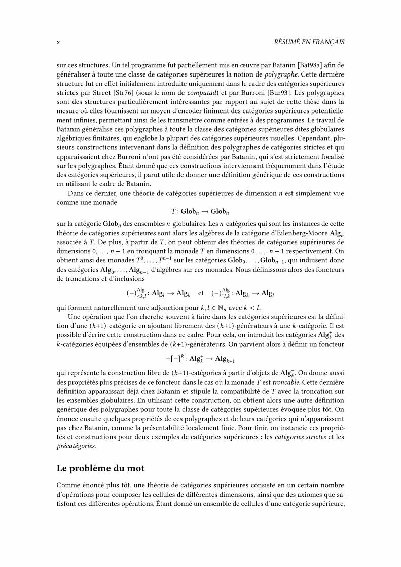
des propriétés plus précises de ce foncteur dans le cas où la monade) est troncable. Cette dernièredé�nition apparaissait déjà chez Batanin et stipule la compatibilité de ) avec la troncation surles ensembles globulaires. En utilisant cette construction, on obtient alors une autre dé�nitiongénérique des polygraphes pour toute la classe de catégories supérieures évoquée plus tôt. Onénonce ensuite quelques propriétés de ces polygraphes et de leurs catégories qui n’apparaissentpas chez Batanin, comme la présentabilité localement �nie. Pour �nir, on instancie ces proprié-tés et constructions pour deux exemples de catégories supérieures : les catégories strictes et lesprécatégories.

Le problème du mot

Comme énoncé plus tôt, une théorie de catégories supérieures consiste en un certain nombred’opérations pour composer les cellules de di�érentes dimensions, ainsi que des axiomes que sa-tisfont ces di�érentes opérations. Étant donné un ensemble de cellules d’une catégorie supérieure,

RÉSUMÉ EN FRANÇAIS xi

il est souvent possible de les composer formellement de plusieurs manières. Le problème du motconsiste alors à déterminer si deux composées formelles de cellules représente la même celluled’après la théorie considérée.

Une solution à ce problème a été donnée par Makkai dans le cas des catégories strictes [Mak05].Cependant, sa solution est relativement ine�cace et ne permet pas de résoudre des instancesconcrètes qui sont trop sophistiquées. Une partie du travail de cette thèse a consisté à améliorerl’algorithme proposé par Makkai en donnant une meilleure description calculatoire des catégoriesstrictes libres. Pour cela, il a fallu clari�er la notion de calculabilité dans le cadre des catégoriessupérieures, ce que nous avons fait en utilisant le formalisme des fonctions récursives. Finalement,nous avons produit une implémentation utilisable de notre algorithme résolvant le problème dumot pour les catégories strictes.

Diagrammes de recollement

Les diagrammes de recollement (pasting diagrams en anglais) sont un outil standard dans l’étudedes catégories strictes et, plus généralement, d’un certain nombre de catégories supérieures. Ilspermettent de désigner une cellule d’une catégorie supérieure simplement en dessinant la façonde recoller les cellules qui la composent sur un diagramme comme le suivant :

D E F G ~0

2

1

3

⇓ U

⇓ V5

4

6

ℎ⇓ W

⇓ X.

Il est en e�et possible de véri�er que toutes les façons de composer les cellules de ce diagrammeinduisent la même cellule, et donc que ce diagramme permet bien de représenter une uniquecellule sans que l’on ait besoin de préciser une composée formelle des cellules la constituant.Cependant, cette propriété n’est pas satisfaite par tous les diagrammes de cellules : certainssont associés à plusieurs compositions formelles di�érentes, et d’autres sont associés à aucunecomposition. Ainsi, a�n de pouvoir utiliser des diagrammes dans l’étude des catégories strictes, ilest important de pouvoir distinguer les diagrammes qui sont associés à une unique composition.Pour cela, trois formalismes di�érents ont été introduits jusqu’à présent : les complexes de parité deStreet [Str91], les schémas de recollement de Johnson [Joh89] et les complexes dirigés augmentésde Steiner [Ste04].

Une partie du travail de cette thèse a consisté à essayer de mieux comprendre les liens entreces di�érents formalismes ainsi que les di�érences entre leurs expressivités. Durant cette étude,il fut découvert que l’axiomatique des complexes de parité et des schémas de recollement étaientdéfectueuses, dans le sens où ces formalismes acceptaient des diagrammes qui n’étaient pas asso-ciés à des compositions formelles uniques. Cela motiva l’introduction d’un nouveau formalisme,appelé complexes sans torsion, généralisant les trois introduits et corrigeant les défauts des com-plexes de parité et des schémas de recollement. Nous avons prouvé en détail la correction de cenouveau formalisme en adaptant et complétant les preuves données par Street pour les complexesde parité. Nous avons ensuite e�ectué la comparaison avec les autres formalismes et montré,selon des restrictions raisonnables, que ceux-ci étaient des cas particuliers de complexes sanstorsion. Pour �nir, nous avons illustré l’utilité de cette nouvelle structure en en fournissant uneimplémentation qui permet de faciliter l’interaction avec le programme résolvant le problème dumot évoqué plus haut.

xii RÉSUMÉ EN FRANÇAIS

Cohérence dans les catégories de Gray

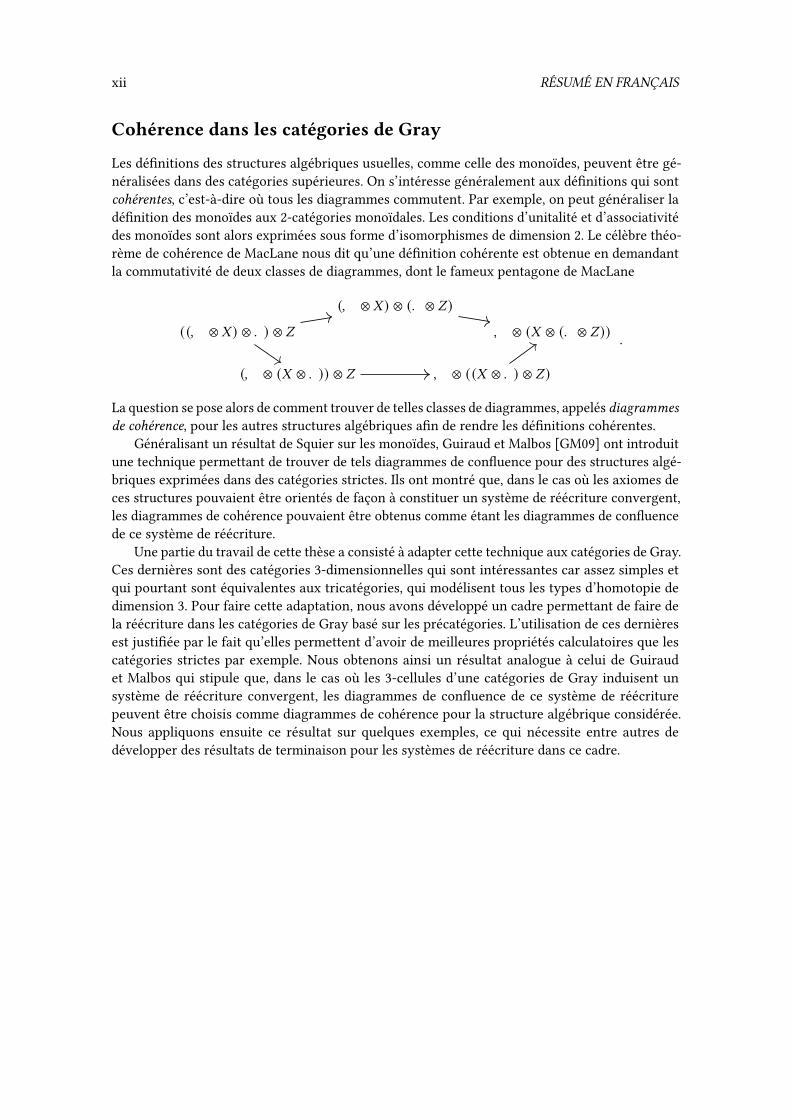
Les dé�nitions des structures algébriques usuelles, comme celle des monoïdes, peuvent être gé-néralisées dans des catégories supérieures. On s’intéresse généralement aux dé�nitions qui sontcohérentes, c’est-à-dire où tous les diagrammes commutent. Par exemple, on peut généraliser ladé�nition des monoïdes aux 2-catégories monoïdales. Les conditions d’unitalité et d’associativitédes monoïdes sont alors exprimées sous forme d’isomorphismes de dimension 2. Le célèbre théo-rème de cohérence de MacLane nous dit qu’une dé�nition cohérente est obtenue en demandantla commutativité de deux classes de diagrammes, dont le fameux pentagone de MacLane

(, ⊗ - ) ⊗ (. ⊗ / )

((, ⊗ - ) ⊗ . ) ⊗ /

(, ⊗ (- ⊗ . )) ⊗ / , ⊗ ((- ⊗ . ) ⊗ / )

, ⊗ (- ⊗ (. ⊗ / )) .

La question se pose alors de comment trouver de telles classes de diagrammes, appelés diagrammesde cohérence, pour les autres structures algébriques a�n de rendre les dé�nitions cohérentes.

Généralisant un résultat de Squier sur les monoïdes, Guiraud et Malbos [GM09] ont introduitune technique permettant de trouver de tels diagrammes de con�uence pour des structures algé-briques exprimées dans des catégories strictes. Ils ont montré que, dans le cas où les axiomes deces structures pouvaient être orientés de façon à constituer un système de réécriture convergent,les diagrammes de cohérence pouvaient être obtenus comme étant les diagrammes de con�uencede ce système de réécriture.

Une partie du travail de cette thèse a consisté à adapter cette technique aux catégories de Gray.Ces dernières sont des catégories 3-dimensionnelles qui sont intéressantes car assez simples etqui pourtant sont équivalentes aux tricatégories, qui modélisent tous les types d’homotopie dedimension 3. Pour faire cette adaptation, nous avons développé un cadre permettant de faire dela réécriture dans les catégories de Gray basé sur les précatégories. L’utilisation de ces dernièresest justi�ée par le fait qu’elles permettent d’avoir de meilleures propriétés calculatoires que lescatégories strictes par exemple. Nous obtenons ainsi un résultat analogue à celui de Guiraudet Malbos qui stipule que, dans le cas où les 3-cellules d’une catégories de Gray induisent unsystème de réécriture convergent, les diagrammes de con�uence de ce système de réécriturepeuvent être choisis comme diagrammes de cohérence pour la structure algébrique considérée.Nous appliquons ensuite ce résultat sur quelques exemples, ce qui nécessite entre autres dedévelopper des résultats de terminaison pour les systèmes de réécriture dans ce cadre.

Remerciements

J’aimerais tout d’abord remercier mes deux directeurs de thèse, Samuel et Yves, qui ont accepté dem’encadrer pendant ces trois années de thèse. Leur disponibilité et leur écoute durant cette périodeont sûrement fait de moi un thésard privilégié. Aussi, mes échanges avec eux m’ont beaucoupappris, notamment sur mon domaine de recherche, mais aussi sur le monde de la recherche engénéral. J’aimerais en particulier remercier Yves pour son soutien lors de la rédaction de monpremier article, et Samuel pour ses blagues qui n’étaient pas toujours mauvaises.

Then, I would like to thank the di�erent people who agreed to be part of my defense jury: TomHirschowitz, François Métayer, Viktoriya Ozornova, Ross Street, Dominic Verity and Jamie Vicary.I am particularly grateful for the attendance of Ross and Dominic given the ten-hour di�erencebetween our two time zones. I am also grateful for the work done by Tom and Dominic, who agreed tobe my rapporteurs and to read my lengthy manuscript in full details. I would also like to thank Rossfor agreeing to be rapporteur in the �rst place, before being refused by my graduate school. I wouldalso like to thank Dimitri Ara for agreeing to be in the jury at some point, even though it was notpossible for him to attend in the end.

J’aimerais maintenant remercier les gens du laboratoire d’informatique de Polytechnique et,plus particulièrement, les gens de l’équipe CoSyNuS avec qui j’ai passé la partie la plus importantede mon temps de doctorat. Je voudrais d’abord remercier Patrick et Thibaut avec qui j’ai partagéun bureau et eu des conversations très intéressantes sur Haskell, HoTT ou autres. Je voudraisaussi remercier Emmanuel pour ses sélections de thés et pour ses anecdotes toujours croustillantes.Un merci aussi à François pour s’être assuré que nous mangions tous en venant nous cherchertous les midis pour aller à la cantine. J’aimerais en�n remercier Bibek, Éric, Maria, Nan, Roman,Sergio, Sylvie et Uli pour les échanges intéressants que l’on a pu avoir, que ce soit au bureau oulors de sessions Zoom après une journée de travail.

Une pensée aussi pour les gens de l’IRIF à l’Université de Paris (anciennement Paris Diderot)que j’aurais aimé voir plus souvent et mieux connaître. Notamment le sympathique groupe dedoctorants qui était présent à ce moment : Axel, Cédric, Chaitanya, Jules, Léo, Léonard, Pierre,Rémi, Théo, Zeinab, et les autres. Des remerciements aussi aux membres permanents, commeFrançois, Pierre-Louis, et Paul-André, qui m’ont aidé à plusieurs reprises et m’ont fait pro�ter deleurs lumières sur les sujets sur lesquels je travaillais.

Ensuite, j’aimerais remercier les gens que j’ai connus avant ma thèse. Je pense d’abord auxpersonnes avec qui j’ai fait mes années d’études en informatique à l’ENS : Andreea, Antoine,Antonin, Baptiste, Christophe, Florent, Ken, Maxime, Thomas, Vincent, et les autres. Je garde un

xiii

xiv REMERCIEMENTS

bon souvenir des moments que l’on a passés ensemble, notamment les sorties au sushi du coin quifurent vraiment (trop) nombreuses, ainsi que les soirées en Info4 que l’on passait à �nir des projetspour lesquels on était à la bourre. J’aimerais aussi remercier les gens du A6, avec qui j’ai vécuune belle expérience de vie en communauté durant l’année 2015-2016 : Axel, Benjamin, Charles,Chloé, Jean1, Jean2, Paul, Quentin, Romain, Salim. J’aimerais en particulier remercier Quentinpour avoir toujours su trouver le courage pour cuisiner pour l’étage en dépit de l’apathie généralequ’il pouvait y avoir pour la préparation des repas du soir quelques fois. Nous ne te méritions pas,Quentin ! J’aimerais aussi remercier Salim de nous avoir invités à passer de très belles vacances auMaroc, malgré les di�érents problèmes d’intoxication alimentaire que nous avons pu y rencontrer.J’aimerais de plus remercier Jean2 pour l’organisation des di�érentes après-midis ou soirées del’étage pour les diverses occasions qui se sont présentées dans l’année. Je le remercie d’avoircontinué cet e�ort après la dissolution forcée du A6 en organisant les « séminaires de la tourTokyo ». Merci aussi aux personnes extérieures mais assimilées au A6 avec qui j’ai pu partagerdes conversations amicales intéressantes : Anne, Julien, Pierre « W. », Vérène, et les autres.

J’aimerais aussi remercier les gens du Chœur PSL, avec qui j’ai vécu des moments musicauxmémorables : Anne, Armine, Arthur1, Arthur2, Avril, Florence, Gabriel, Julia, Marie, Mathieu,Mathilde, Philomène, Pierre, et les autres. Je pense notamment au concert où nous avons chantéla Passion selon Saint-Jean de Bach, à celui où nous avons chanté le Requiem de Brahms, ainsique les tournées en Bretagne et à Londres. J’espère pouvoir revivre des expériences musicalesaussi intenses un jour mais cela risque d’être di�cile. Je souhaite bien sûr remercier Johan, le chefd’orchestre, pour nous avoir fait découvrir tous ces beaux morceaux.

La famille maintenant. J’aimerais d’abord remercier ma mère pour son soutien indéfectibledurant cette période, malgré les soucis beaucoup plus graves qui l’a�igeaient par ailleurs. J’aime-rais aussi remercier ma sœur, qui a aussi toujours été présente pour moi et avec qui j’ai pu trouverdes moments pour me détendre à Paris à l’occasion de séances de cinéma ou de dégustation depâtisseries dans des salons de thé. Merci aussi au reste de ma famille pour les di�érents momentsqu’on a passés ensemble durant ces dernières années : Jean-Luc, Bernard et Angelica, Stéphane,Jérôme et Barbara et la famille de Nice.

Pour terminer, j’aimerais remercier quelques inclassables : Charlène, pour toutes les foisoù l’on s’est marré depuis le lycée ; Vincent, pour avoir été un colocataire décent et m’avoirdépanné plusieurs fois en LATEX; Philippe Malbos, pour son aide dans ma recherche infructueusede post-doc à Lyon ; Spacemacs, pour avoir rendu techniquement possible d’écrire ce manuscriten quelques mois ; Philipp H. Poll, pour avoir conçu et mis à disposition sous licence publiquela police Linux Libertine qu’utilise ce document ; et en�n, SRAS-CoV-2/COVID-19 pour m’avoirfourni des conditions optimales pour la rédaction de ce manuscrit, sans distractions extérieurespossibles, et donné l’occasion de passer de longues semaines en famille à la campagne.

Notations

In this thesis, we use the following notations:

– l denotes the smallest in�nite ordinal,

– N denotes the set of natural integers and N∗ denotes the set N \ {0},

– given = ∈ N, N= denotes the set {0, . . . , =} and N∗= denotes the set {1, . . . , =},

– we extend the previous notation to in�nity by putting Nl = N and N∗l = N∗,

– in accordance with the above notations, given = ∈ N ∪ {l}, we often write N= ∪ {=} todenote either N= when = ∈ N, or N ∪ {l} when = = l ,

– given a product∏8∈� -8 of objects -8 of some category indexed by the elements of a set � ,

we write c 9 :∏8∈� -8 → - 9 for the projection on the 9-component for 9 ∈ � ,

– given a coproduct∐8∈� -8 of objects -8 of some category indexed by the elements of a set � ,

we write ] 9 :∐8∈� -8 → - 9 for the coprojection on the 9-component for 9 ∈ � .

xv

Introduction

The sophistication of modern mathematics incites to take into account not only the mathematicalobjects at stack, but also the way they interact, the interaction between those interactions, andso on. We have entered a higher-dimensional approach to the mathematical world. The algebraicstructures involved in such studies, called higher categories, are becoming more and more complexand computationally involved. The aim of this PhD thesis is to introduce several computationaltools to assist with the manipulation of some of these higher categories.

We shall �rst give some general background about this work before introducing the topics of thisthesis in more details.

General background

Higher categories. The beginnings of category theory can be traced back to the 1940s, with thework of Eilenberg and MacLane in algebraic topology, when they investigated the notion of naturaltransformation [EM42; EM45]. A category is a simple structure: objects (or 0-cells) and arrows (or1-cells) between them that can be composed associatively by a binary operation, together with anidentity arrow for each object. Yet, its generality allowed it to become an important abstractiontool in modern mathematics, physics and computer science, for considering algebraic structuresequipped with some notion of composition [BS10].

Even though the scope of categories is broad, there are some situations where they fail toapply. One kind of such situations is when there is additional structure, such as other composi-tion operations, that does not �t in the structure of a category. This is the case when describingcategories themselves: categories and functors form a category, but this description does notencompass the natural transformations between functors and the associated composition opera-tions (the one with between functors and natural transformations, and the one between naturaltransformations). Another kind of situtations is when the unitality and associativity properties ofthe composition operation of categories are too strong. For example, when considering the pathson some topological space - , two paths can be composed by concatenation, but this operation isthen neither unital nor associative. Of course, one can instead consider the paths up to homotopy,for which the above composition operation is unital and associative, and obtain the category ofpaths up to homotopy of - , called the fundamental groupoid of - . But one might still be inter-ested in representing the structure of these homotopies, for which categories are not expressiveenough, so that we fall back into the �rst situation.

xvii

xviii INTRODUCTION

A better treatment of the two above situations can be obtained by considering generalizationsof the notion of category that have higher cells, i.e., (8+1)-cells between 8-cells for 8 ≥ 1, andseveral composition operations for the di�erent cells that can satisfy multiple axioms. We callhigher category an instance of this informal class of structures, and call =-category a higher cate-gory that has cells up to dimension =. The two above situations can then be properly representedby considering the adequate notion of higher category. For instance, the categories, functors,natural transformations and the di�erent compositions between them �t in a strict 2-category,which is a 2-category with unital and associative compositions of the 1- and 2-cells, �rst intro-duced by Ehresmann [Ehr65]; the paths on the space - and their homotopies �t in a bicategory,which is 2-category whose composition of 1-cells is associative up to a 2-cell, introduced byBénabou [Bén67].

By de�nition, there is an in�nity of notions of higher categories. Indeed, the di�erent notionscan di�er with regard to the maximal dimension of cells which are handled, the shape of the cells(globular, cubical, simplicial, etc.), the operations allowed on these cells, and the axioms satis�edby these operations. Each notion of higher category is usually informally situated in the strict-weak spectrum: the higher categories whose axiomatic consists of equalities between compositesof cells are called strict, whereas the ones whose axiomatic consists of the existence of coherencecells between two composites of cells are called weak. For example, categories and strict 2-cate-gories require that the composition of 1-cells be strictly associative, and thus lie on the ‘strict’ sideof the strict-weak spectrum, whereas bicategories require the mere existence of invertible 2-cellsbetween 1-cells composed using di�erent parenthesizing schemes (e.g., there exists a coherence2-cell between (D∗0E)∗0F andD∗0 (E∗0F) for composable 1-cellsD, E,F ), and thus lie on the ‘weak’side of the strict-weak spectrum. Strict higher categories have usually simpler de�nitions andare easier to work with, but, as suggested above, they are not adequate for encoding homotopicalinformation, and one usually turns to weak higher categories for such matters. The downside isthat the axiomatics of weak higher categories are usually technically quite involved, the situationbecoming worse and worse as the dimension of the considered categories increases because ofthe multiple coherence cells between the composition operations [GPS95]. Indeed, in additionto the already evoked coherence cells for associativity, particular de�nitions of weak categoriescan also involve coherence cells for identities, that witness that identities are weakly unital, andexchange coherence cell, that witness that two parallel cells that appear one after the other insome cell can be exchanged, and many more. All these coherence cells should moreover satisfyseveral compatibility conditions which are di�cult to list exhaustively.

In between those two ends of the spectrum, there is the so-called semi-strict de�nitions ofhigher categories, which involve a balanced mixture of strict equations and coherence cells,so that such higher categories are expressive enough for encoding homotopical information,while keeping the complexity of the axiomatic at bay. Notably, in dimension 3, a fundamentalresult of Gordon, Power and Street [GPS95] is that tricategories, the 3-dimensional analogues ofbicategories, are equivalent (for the right notion of equivalence) to semi-strict 3-categories calledGray categories. The latter are ‘strict’ in every respect except for the exchange of 2-cells. Otherinteresting semi-strict 3-categories are the ones that we call Kock categories, which were shown tocorrectly model 3-dimensional homotopical properties [JK06]. Those are ‘strict’ in every respectexcept that identities are only weakly unital. See Figure 1 for a comparison of the axiomatics ofthe 3-dimensional categories introduced so far. Similar semi-strict de�nitions are still looked forin higher dimensions, even though some propositions were made [BV17].

The case for strict categories. Even though strict categories do not represent as well homotopi-cal properties as weak categories, there are still interesting objects that are worth studying. First,they have already found several applications. As remarked by Burroni [Bur93], strict 3-categories

GENERAL BACKGROUND xix

3-categories unitality associativity exchange

strict categories equality equality equalityGray categories equality equality coherence cellKock categories coherence cell equality equalityweak categories coherence cell coherence cell coherence cell

Figure 1 – Strict-weak characteristics of some 3-dimensional categories

can be used as a framework which generalizes classical term rewriting systems, and this factmotivated the interpretation of =-categories for = ≥ 4 as “higher rewriting systems”. This idealed to several developments and applications [Laf03; Mim14; CM17]. In a related manner, strictcategories found some applications in the study of homological properties of monoids, mainly inthe work of Guiraud and Malbos [GMM13; GGM15; GM18]. Moreover, strict categories play a rolein the de�nition of other (possibly weak) higher categories. For example, Gray categories can bede�ned from the Gray tensor product, which is a construction on strict 2-categories. Another ex-ample is the notion of globular operad, developed by Batanin and Leinster [Bat98b; Lei98], whichis a device based on strict categories that allows de�ning other higher categories. In particular,weak categories admit an elegant de�nition in this setting [Lei04]. In a related manner, Henry wasable to de�ne semi-strict higher categories which exhibit the same good homotopical propertiesof weak categories using several constructions on strict categories [Hen18]. Finally, as suggestedby Ara and Maltsiniotis [AM18], since weak categories are quite complicated objects which arehard to manipulate, the study of properties and constructions on strict categories, as a simplercase, seems a necessary step before considering the general case of weak categories.

In addition to the above motivations and applications, strict categories exhibit some niceproperties which make them more pleasant to work with than other higher categories. In partic-ular, they possess a graphical language which enables to easily consider cells that are compositesof other cells. Indeed, whereas one introduce such composites in a general higher-dimensionalcategory by expressions which precisely state how some given cells are composed, it is oftenenough, in strict categories, to simply draw these cells. For example, in usual categories, i.e., strict1-categories, a diagram like

G0 G1 · · · G=−1 G=51 52 5=−1 5= (1)

which represents a sequence of 1-cells 51, . . . , 5= of some category � unambiguously de�nes “the”composite of 51, . . . , 5= . This is simply a consequence of the fact that the composition of 1-cells isassociative, so that all the expressions one can think of to compose the 58 ’s together are equivalent.This property, which is rather trivial for 1-categories, generalizes to higher dimensions, so that,for example, a diagram like

F

E G ~ I

10

2

3

4

5

6

⇓U ⇓V

⇓W

can be used to de�ne unambiguously a 2-cell in some strict 2-category, thus without the needfor an explicit expression which states precisely how to compose the generators of the diagramtogether. Such diagrams are called pasting diagrams, since they express how a given set of cells of

xx INTRODUCTION

a strict category are “pasted” together. They �rst appeared for strict 2-categories in the work ofBénabou [Bén67]. The use of such pasting diagrams facilitate the manipulation of strict categoriesand is widespread in the literature about these categories.

Computability. The notion of computation appeared long before the �rst modern computers.Written calculation procedures were identi�ed on Babylonian clay tablets [Knu72] (circa 1600 B.C.)and some well-known arithmetical algorithms still used today were invented in ancient Greece,like Euclid’s algorithm and the sieve of Eratosthenes (circa 300 B.C.). But it was only in the 20thcentury that the notions of computation and computability were seriously formalized. In 1923,Skolem �rst de�ned a class of functions that can be computed by �nite procedures [Sko23],now known as primitive recursive functions. Later, Gödel gave a more general class of computablefunctions [Göd34], now known as recursive functions. Other models of computation were proposedat the time, like Church’s lambda calculus [Chu36] and Turingmachines [Tur36], that in fact turnedout to be equivalent to recursive functions. This led to the introduction of the Church-Turingthesis, which asserts that any “computable procedure” can be expressed in one of these models.

The latter were introduced in order to provide answers to foundational problems of mathe-matics raised by Hilbert and others at the time. On the one hand, Hilbert’s second problem askedwhether the axiomatic of arithmetics could be shown consistent, considering the advances in thelogical aspects of mathematics at the time. Using his formalism of primitive recursive functions,Gödel provided a negative answer to this question, in the form of his famous incompletenesstheorem. On the other hand, Hilbert and Ackermann’s Entscheidungsproblem (“decision problem”)asked whether there existed a general computable procedure that would decide whether a givenmathematical statement is true or false. Church and Turing gave two di�erent negative answersto this question, by showing more generally the existence of undecidable problems, i.e., problemsthat can not be solved by computable procedures. In particular, Turing showed that the haltingproblem, i.e., the problem that consists in deciding whether a given Turing machine stops after a�nite number of steps, was undecidable.

Since then, a lot of other undecidable problems were discovered. The proof of undecidability ofa given problem usually relies on reducing the halting problem or some other known undecidableproblem to it. A common source for undecidable problems are the word problems associatedwith presentations. Recall that mathematical objects are often de�ned by means of presentations,i.e., as sets of generators that can be combined into terms, or words, such that the evaluationof these terms satisfy several equations. In particular, monoids can be de�ned by presentations,where the words that appear in the equations are simply sequences of generators. For example,the monoid (N2, (0, 0), +) can be presented as the monoid induced by two generators 0 and 1satisfying the equation 01 = 10. Instances other algebraic theories (groups, rings, etc.) can bepresented by a similar fashion. In fact, theories themselves are usually de�ned by means ofpresentations. The words in this case are �nite trees which represent expressions that can bewritten in the considered theory. For example, the theory of monoids can be presented as thetheory of structures consisting in a unit 4 and a binary operation rsuch that the equations

4 rG = G G r4 = G (G r~) rI = G r (~ rI)are satis�ed for all elements G,~, I of the structure. Other algebraic theories can be presented in asimilar fashion. Given any kind of presentation, the word problem consists in deciding whethertwo given words are equal with regard to the equations of the presentation. Before the appearanceof recursive functions and the other computation models, it was already asked whether thereexisted a procedure to decide the word problem for presentations of groups by Dehn [Deh11],and for presentation of monoids by Thue [Thu14]. It was shown not to be the case, since there

GENERAL BACKGROUND xxi

are examples of presentations with undecidable word problems: this was shown by Post [Pos47]and Markov [Mar47] for monoids, and by Novikov [Nov55] for groups.

Rewriting. Even though there is no general procedure to solve the word problem for all pre-sentations of monoids, groups, theories, etc. solutions might exist for some presentations. Inparticular, one can derive a solution to the word problem when the considered presentation isassociated with a rewriting system with good properties. Formally, one obtains a rewriting systemfrom a presentation by simply orienting the equations of the presentation. Such orientationsshould be thought as de�ning a set of allowed moves, or rewrite rules, from a word to another.In order for the rewriting system to exhibit good properties, the orientations of the equationsshould be chosen so that the word obtained after applying a rewrite rule is simpler than the wordone started from. The de�nition of “simpler” here is relative to each situation. It can mean forexample “being smaller” or “being better bracketed” (on the left or on the right, depending onconvention). By combining all the rewrite rules, one then obtains a rewrite relation on the words.For example, one can orient the equations of the theory of monoids as follows:

4 rG ⇒ G G r4 ⇒ G (G r~) rI ⇒ G r (~ rI).The above rewrite rules induce a rewrite relation⇒ for which we have the rewrite sequence

(G r (~ r4)) r (I r4) ⇒ (G r~) r (I r4) ⇒ (G r~) rI ⇒ G r (~ rI)where the �nal word is simpler than the one we started from.

Once a rewriting system is introduced for a presentation, one can try a normal form strategyto solve the word problem: given two words that are to be compared, we reduce both wordswith the rewrite relation until they can not be reduced further, and then compare the resultingnormal forms. For this strategy to work, several additional conditions should be satis�ed. First,the rewriting system should have a �nite number of rewrite rules, so that we are able to detectwhen we have found a normal form. Moreover, the rewrite relation⇒ should be terminating, i.e.,it should not allow in�nite rewrite sequences. Finally, the relation⇒ should satisfy a propertyof con�uence, which states that all the di�erent possible rewrite sequences starting from a givenword lead to the same normal form. When these conditions are satis�ed, the normal form strategyprovides a computational procedure which solves the word problem.

The aim of rewriting theory is, among others, to provide generic criteria for showing severalproperties of rewrite relations, including termination and con�uence, even though such proper-ties are undecidable in general [Ter03]. In particular, as a consequence of two classical results,namely Newman’s lemma and the critical pair lemma, the con�uence of a terminating rewriterelation reduces to the con�uence of rewrite sequences associated to the critical branchings of therewriting system: those are pairs of the generating rewrite rules that are minimally overlapping.The con�uence of the theory of monoids can be deduced this way, since the associated rewriterelation can be shown terminating, and since moreover each of its critical branching can be showncon�uent. For example, this theory admits the critical branching

(F r (G r~)) rI ⇐ ((F rG) r~) rI ⇒ (F rG) r (~ rI)and this branching is witnessed con�uent by the diagram

(F rG) r (~ rI)((F rG) r~) rI

(F r (G r~)) rI F r ((G r~) rI)F r (G r (~ rI)) . (2)

xxii INTRODUCTION

The use of con�uent and terminating rewriting systems for providing a decidable solution tothe word problem naturally led to the question, initially raised by Jantzen [Jan84], of whether anymonoid with decidable word problem can be presented by a �nite terminating con�uent rewritingsystem, so that the normal form strategy apply. This question was answered by Squier [Squ87].He showed that monoids which can be presented with �nite terminating con�uent rewritingsystems satisfy a �niteness homological property which does not depend on the presentation.He then gave an example of a monoid which has a decidable word problem but does not satisfythis homological condition, answering negatively Jantzen’s question. The work of Squier on thisproblem had deep consequences, since it establishes a link between presentations and homologicalinvariants of monoids. In fact, this connection extends to homotopical invariants of monoids, aswas shown in a posthumous article [SOK94]. The latter result formalizes the idea that con�uencediagrams of critical branchings like (2) are the elementary “holes” of a space associated to apresented monoid.

Coherence. In mathematics, coherence properties are an informal class of results which canappear in various contexts and take di�erent forms. Maybe one of the �rst coherence result isthe coherence of an associative binary operation [Bou07, Théorème 1]. This result states that,given a binary operation ron a set which satis�es that (G r~) rI = G r(~ rI), one does not need toparenthesize an expression G1 r · · · rG= since all parenthesizing schemes induce the same result.This is a fundamental fact about associative operations that is used daily by most mathematicians.More generally, coherence properties assert that the choices we can have in using the operationsof some structure do not matter in the end, since all possible choices lead to the same result.

Coherence results are particularly present in (higher) category theory. They usually ap-pear when considering weakened versions of algebraic structures expressed in some category.Such weakened versions are obtained by replacing the equalities of the algebraic theories byisomorphisms. A classical example is monoidal categories, which are weakened monoids, orpseudomonoids, expressed in the category of categories. The “associativity” here takes the formof isomorphisms

(- ⊗ . ) ⊗ / → - ⊗ (. ⊗ / )

which allow to change the bracketing. Given a sequence of objects -1, . . . , -= , there are thendi�erent possible ways one can use the above associativity morphisms to relate the left and rightbracketings

((· · · (-1 ⊗ -2) ⊗ · · · ) ⊗ -=−1) ⊗ -= -1 ⊗ (-2 ⊗ (· · · ⊗ (-=−1 ⊗ -=) · · · )).

MacLane’s coherence theorem for monoidal categories [Mac63] asserts that all the di�erent iso-morphisms one can build between the two above objects using the associativity isomorphismsare equal. The proof of this fact reduces to the commutation of the pentagon diagrams

(, ⊗ - ) ⊗ (. ⊗ / )

((, ⊗ - ) ⊗ . ) ⊗ /

(, ⊗ (- ⊗ . )) ⊗ / , ⊗ ((- ⊗ . ) ⊗ / )

, ⊗ (- ⊗ (. ⊗ / )) (3)

which is required by the de�nition of monoidal categories. Several coherence results wereproved for other weak structures: symmetric monoidal categories [Mac63], braided monoidalcategories [JS93], Frobenius pseudomonoids [DV16], etc. Like MacLane’s theorem, these coher-ence properties are the consequence of the commutation of a �nite number of classes of diagrams,that we call coherence tiles, which are required by the de�nitions of the structures. In fact, the

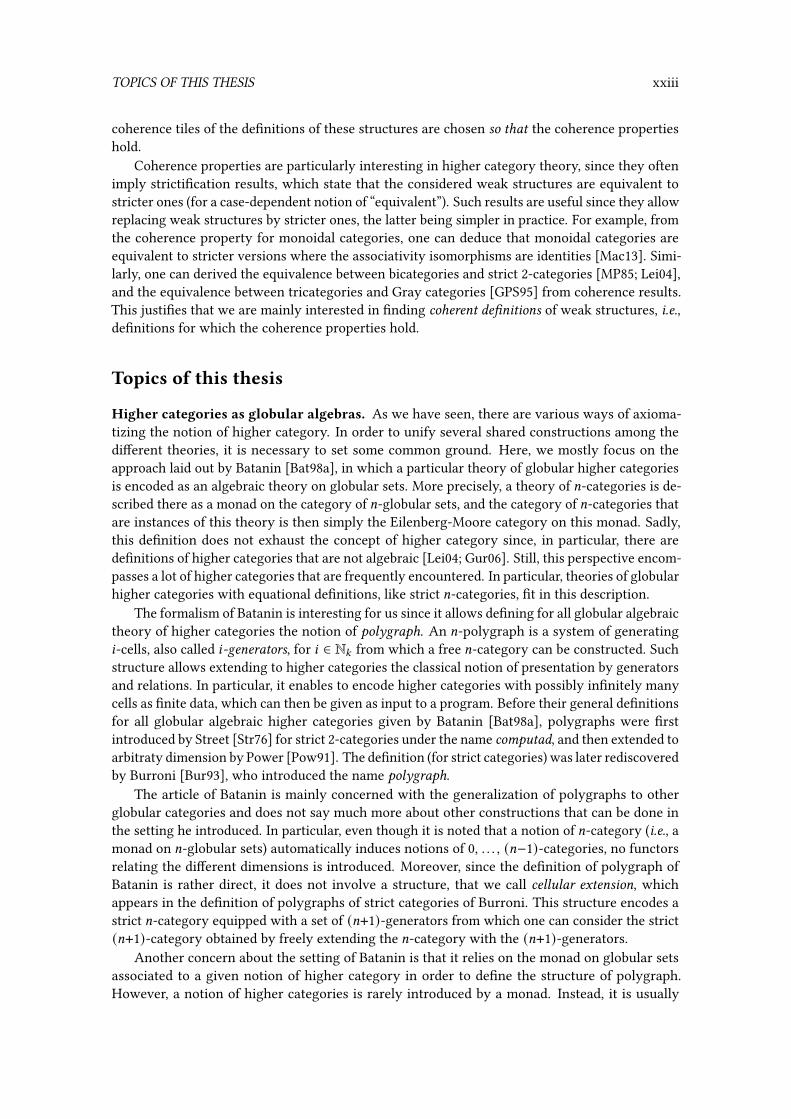
TOPICS OF THIS THESIS xxiii

coherence tiles of the de�nitions of these structures are chosen so that the coherence propertieshold.

Coherence properties are particularly interesting in higher category theory, since they oftenimply stricti�cation results, which state that the considered weak structures are equivalent tostricter ones (for a case-dependent notion of “equivalent”). Such results are useful since they allowreplacing weak structures by stricter ones, the latter being simpler in practice. For example, fromthe coherence property for monoidal categories, one can deduce that monoidal categories areequivalent to stricter versions where the associativity isomorphisms are identities [Mac13]. Simi-larly, one can derived the equivalence between bicategories and strict 2-categories [MP85; Lei04],and the equivalence between tricategories and Gray categories [GPS95] from coherence results.This justi�es that we are mainly interested in �nding coherent de�nitions of weak structures, i.e.,de�nitions for which the coherence properties hold.

Topics of this thesis

Higher categories as globular algebras. As we have seen, there are various ways of axioma-tizing the notion of higher category. In order to unify several shared constructions among thedi�erent theories, it is necessary to set some common ground. Here, we mostly focus on theapproach laid out by Batanin [Bat98a], in which a particular theory of globular higher categoriesis encoded as an algebraic theory on globular sets. More precisely, a theory of =-categories is de-scribed there as a monad on the category of =-globular sets, and the category of =-categories thatare instances of this theory is then simply the Eilenberg-Moore category on this monad. Sadly,this de�nition does not exhaust the concept of higher category since, in particular, there arede�nitions of higher categories that are not algebraic [Lei04; Gur06]. Still, this perspective encom-passes a lot of higher categories that are frequently encountered. In particular, theories of globularhigher categories with equational de�nitions, like strict =-categories, �t in this description.

The formalism of Batanin is interesting for us since it allows de�ning for all globular algebraictheory of higher categories the notion of polygraph. An =-polygraph is a system of generating8-cells, also called 8-generators, for 8 ∈ N: from which a free =-category can be constructed. Suchstructure allows extending to higher categories the classical notion of presentation by generatorsand relations. In particular, it enables to encode higher categories with possibly in�nitely manycells as �nite data, which can then be given as input to a program. Before their general de�nitionsfor all globular algebraic higher categories given by Batanin [Bat98a], polygraphs were �rstintroduced by Street [Str76] for strict 2-categories under the name computad, and then extended toarbitraty dimension by Power [Pow91]. The de�nition (for strict categories) was later rediscoveredby Burroni [Bur93], who introduced the name polygraph.

The article of Batanin is mainly concerned with the generalization of polygraphs to otherglobular categories and does not say much more about other constructions that can be done inthe setting he introduced. In particular, even though it is noted that a notion of =-category (i.e., amonad on =-globular sets) automatically induces notions of 0, . . . , (=−1)-categories, no functorsrelating the di�erent dimensions is introduced. Moreover, since the de�nition of polygraph ofBatanin is rather direct, it does not involve a structure, that we call cellular extension, whichappears in the de�nition of polygraphs of strict categories of Burroni. This structure encodes astrict =-category equipped with a set of (=+1)-generators from which one can consider the strict(=+1)-category obtained by freely extending the =-category with the (=+1)-generators.

Another concern about the setting of Batanin is that it relies on the monad on globular setsassociated to a given notion of higher category in order to de�ne the structure of polygraph.However, a notion of higher categories is rarely introduced by a monad. Instead, it is usually

xxiv INTRODUCTION

presented, like other algebraic theories, as a structure with operations satisfying several equations.Even though the task of describing the associated monad is not conceptually di�cult, it is stilltedious and one usually prefers avoiding it. But some properties introduced by Batanin oftenrequire verifying that the considered monad is truncable, i.e., exhibits some compatibility with thetruncation operations on globular sets, so that it seems di�cult to escape an explicit descriptionof the monad at �rst glance. These technicalities likely hinder a wider use of the general resultsthat can be formulated in the setting of Batanin.

Word problem. Like usual free algebraic objects, the cells of the =-category freely generated onan =-polygraph can be described by words which combine the generators of the polygraphs withthe operations the considered theory of =-category. Since these operations can be required tosatisfy several axioms, there are usually several words that can represent the same cell. The wordproblem on polygraphs of higher categories consists in deciding whether two words represent thesame cell. Solving this problem is important for providing e�cient computational descriptionsand helping with the study of higher categories.

Given the role that strict categories play in higher categories, �nding an e�cient and usablesolution to the word problem on (polygraphs of) strict categories is particularly important. In thiscontext, it seems that the usual normal form strategy can not be applied, since there is no knownorientation of the axioms of strict categories that would induce a con�uent and terminatingrewriting system. In [Mak05], Makkai gave a solution to this problem. He showed that, eventhough there is no known unique normal form for the words, they still admit canonical forms.Moreover, the canonical forms of two equivalent words can be related by a sequence of moves,and these canonical forms can be enumerated by a terminating procedure. This solves the wordproblem, since two words are equivalent if and only if they have canonical forms which can berelated by a sequence of moves. However, the resulting procedure is computationally expensiveand quickly overwhelmed by rather simple instances (Makkai deemed himself its procedure as“infeasible”), which prevents its use on concrete instances.

The work of Makkai revealed that the canonical forms for the cells exist for a more primitivestructure than the one of strict =-category, that we call =-precategory: the latter are a variantof strict categories that do not satisfy the exchange identity of strict categories (c.f. Figure 1).The word problem on polygraphs of precategories then admits a simple solution: two wordsare equivalent if they have the same unique canonical form. These good computational proper-ties motivate searching for other situations in which =-precategories can be used. Interestingly,they are already the underlying structure of Globular, a diagrammatic proof assistant for highercategories [BKV16; BV17].

The article of Makkai on the word problem [Mak05] introduced several notions and toolsthat are of more general interest to the study of strict categories. In particular, he introduced a“content function”, that we call Makkai’s measure, which assesses the complexity of the cells ofstrict categories freely generated on polygraphs. More precisely, this function gives some accounton how many times each generator of the polygraph is used in the de�nition of a given cell. Thisfunction admits a simple inductive de�nition and moreover possesses several good properties.Makkai used it to show that his procedure which computes all the canonical forms of a given wordterminates. His measure appears to have one shortcoming though: it counts multiple times low-dimensional generators. This defect raised the question, formulated by Makkai, of the existence ofanother measure that would not display this bad behavior. The existence of such a measure wouldbe useful, since it could help to characterize a class of polygraphs called computopes by Makkai,and later studied by Henry [Hen17] under the name polyplexes, which seem to play an importantrole in the study of polygraphs. In particular, they were used to show that some subcategories ofthe category of polygraphs are presheaf categories or not [Mak05; Hen17].

TOPICS OF THIS THESIS xxv

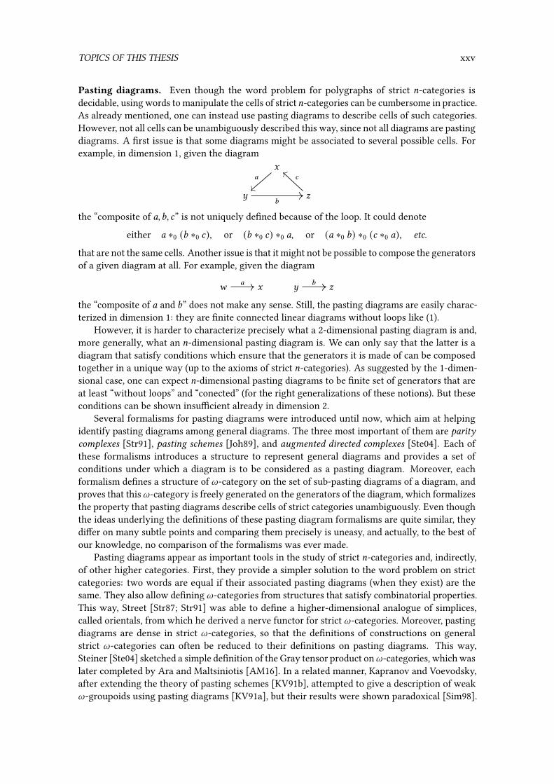
Pasting diagrams. Even though the word problem for polygraphs of strict =-categories isdecidable, using words to manipulate the cells of strict=-categories can be cumbersome in practice.As already mentioned, one can instead use pasting diagrams to describe cells of such categories.However, not all cells can be unambiguously described this way, since not all diagrams are pastingdiagrams. A �rst issue is that some diagrams might be associated to several possible cells. Forexample, in dimension 1, given the diagram

G

~ I

0

1

2

the “composite of 0, 1, 2” is not uniquely de�ned because of the loop. It could denote

either 0 ∗0 (1 ∗0 2), or (1 ∗0 2) ∗0 0, or (0 ∗0 1) ∗0 (2 ∗0 0), etc.

that are not the same cells. Another issue is that it might not be possible to compose the generatorsof a given diagram at all. For example, given the diagram

F G ~ I0 1

the “composite of 0 and 1” does not make any sense. Still, the pasting diagrams are easily charac-terized in dimension 1: they are �nite connected linear diagrams without loops like (1).

However, it is harder to characterize precisely what a 2-dimensional pasting diagram is and,more generally, what an =-dimensional pasting diagram is. We can only say that the latter is adiagram that satisfy conditions which ensure that the generators it is made of can be composedtogether in a unique way (up to the axioms of strict =-categories). As suggested by the 1-dimen-sional case, one can expect =-dimensional pasting diagrams to be �nite set of generators that areat least “without loops” and “conected” (for the right generalizations of these notions). But theseconditions can be shown insu�cient already in dimension 2.

Several formalisms for pasting diagrams were introduced until now, which aim at helpingidentify pasting diagrams among general diagrams. The three most important of them are paritycomplexes [Str91], pasting schemes [Joh89], and augmented directed complexes [Ste04]. Each ofthese formalisms introduces a structure to represent general diagrams and provides a set ofconditions under which a diagram is to be considered as a pasting diagram. Moreover, eachformalism de�nes a structure of l-category on the set of sub-pasting diagrams of a diagram, andproves that thisl-category is freely generated on the generators of the diagram, which formalizesthe property that pasting diagrams describe cells of strict categories unambiguously. Even thoughthe ideas underlying the de�nitions of these pasting diagram formalisms are quite similar, theydi�er on many subtle points and comparing them precisely is uneasy, and actually, to the best ofour knowledge, no comparison of the formalisms was ever made.

Pasting diagrams appear as important tools in the study of strict =-categories and, indirectly,of other higher categories. First, they provide a simpler solution to the word problem on strictcategories: two words are equal if their associated pasting diagrams (when they exist) are thesame. They also allow de�ning l-categories from structures that satisfy combinatorial properties.This way, Street [Str87; Str91] was able to de�ne a higher-dimensional analogue of simplices,called orientals, from which he derived a nerve functor for strict l-categories. Moreover, pastingdiagrams are dense in strict l-categories, so that the de�nitions of constructions on generalstrict l-categories can often be reduced to their de�nitions on pasting diagrams. This way,Steiner [Ste04] sketched a simple de�nition of the Gray tensor product onl-categories, which waslater completed by Ara and Maltsiniotis [AM16]. In a related manner, Kapranov and Voevodsky,after extending the theory of pasting schemes [KV91b], attempted to give a description of weakl-groupoids using pasting diagrams [KV91a], but their results were shown paradoxical [Sim98].

xxvi INTRODUCTION

Coherence for Gray categories. In order to make a weakened de�nition of some algebraicstructure expressed in a higher category coherent, one faces the problem of �nding a correct setof coherence tiles. Recently, it was shown by Guiraud and Malbos [GM09] that, in the contextof strict categories, these coherence tiles can be found using an extension of Squier theorems to“higher rewriting systems” on strict categories.

A higher rewriting system in their setting is simply a polygraph of strict categories. Indeed,it was noted by Burroni when he introduced his de�nition of polygraphs [Bur93] that polygraphsgeneralize the classical notion of rewriting system. For example, one can encode the earlierintroduced rewriting system of the theory of monoids as the 3-polygraph with two 2-generators

and

representing the generating operations of the theory of monoids, and three 3-generators

L : V R : V A : V

representing the rewrite rules of the rewriting system. This motivated the interpretation ofpolygraphs of higher dimensions as higher-dimensional rewriting systems, for which the classicalresults from rewriting theory, and even Squier theorems, can be adapted.

In particular, when searching for a coherent de�nition of a weakened algebraic theory ex-pressed in strict categories, if this theory is presented by a �nite, con�uent and terminating higherrewriting system, one can choose the coherence tiles to be the con�uence diagrams of the criticalbranchings of this rewriting system. For instance, Guiraud and Malbos showed that the coher-ence tiles of monoidal categories can be derived from the critical branchings of an associatedrewriting system, as already suggested by the resemblance between (2) and (3). Even thoughseveral additional conditions need to be proved in each situation, like the termination and thecon�uence of the associated rewriting system, this still provides a generic method for �ndingcoherent weakened de�nitions of algebraic structures expressed in strict categories.

Adaptations of this method would be useful in order to �nd coherent de�nitions in otherhigher categories, in particular weak categories. Since bicategories (i.e., weak 2-categories) areequivalent to strict 2-categories, which are already handled by the framework of Guiraud andMalbos, tricategories are the �rst interesting case. But tricategories are complicated objects, forwhich the development of rewriting techniques might prove di�cult. However, since tricategoriesare equivalent to the simpler Gray categories, it is enough to adapt the tools of Guiraud and Malbosfor the latter. These tools could be used to recover existing coherent de�nitions of weak structuresfor Gray categories, like pseudomonoids or pseudoadjunctions [Lac00; Dos18] and �nd new ones.

In order to adapt these tools, the development of a rewriting framework for Gray categoriesis required. Since the latter have exchange coherence cells (c.f. Figure 1) that might interactwith the operations of the studied weakened de�nitions, it is useful to consider a more primitivestructure as the underlying rewriting setting. A good candidate are precategories, which wealready mentioned earlier. Indeed, they admit a simple computational representation and theirword problem is trivial. Moreover, they do not require the exchange identity of strict categories,which was shown problematic in the context of higher rewriting since it allows a �nite rewritingsystem to have an in�nite number of critical branchings [Laf03; Mim14], which prevents theirexhaustive enumeration by a computer.

Outline of the thesis. The object of this thesis is the introduction of several computationaltools for strict categories and Gray categories. It is organized around three main topics: the wordproblem for strict categories, the pasting diagram formalisms, and the coherence problem forGray categories. The detailed structure of this manuscript follows.

TOPICS OF THIS THESIS xxvii

In Chapter 1, we recall the formalization, given by Batanin [Bat98a], of higher categoriesas globular algebras, and derive several constructions and de�nitions, like the one of polygraph.Then, we introduce the equational de�nitions of the two theories of higher categories that willmainly concern us during this thesis: strict =-categories and =-precategories. In order to obtainall the properties and constructions given by the framework of Batanin, we will have to showthat these theories are derived from monads on globular with su�cient properties. In order toavoid the tedious task of explicitly describing the monads of each theory, we introduce criteriaon the categories of algebras to decide whether these algebras are derived from adequate monadson globular sets.

In Chapter 2, we revisit the solution to the word problem on strict =-categories given byMakkai in [Mak05]. For this purpose, we recall the de�nition of Makkai’s measure for suchpolygraphs, by deriving it from another measure de�ned by Henry [Hen18]. Using an equivalentdescription of strict categories as precategories satisfying some exchange condition, we providea syntactical description of the free =-categories which is amenable to computation. From thisdescription, we derive a solution to the word problem which is a more e�cient version of the onegiven by Makkai, and give an implementation for it. Finally, we answer the question raised byMakkai and show by the mean of a counter-example the nonexistence of a measure on polygraphsthat does not double-count generators.

In Chapter 3, we study the pasting diagrams for strict categories and consider the three mainexisting formalisms for them, namely parity complexes, pasting schemes and augmented directedcomplexes. We show that the axiomatics of parity complexes and pasting schemes are �awed,in the sense that they do not guarantee that the cells of strict categories can be representedfaithfully by the diagrams which these formalisms consider as pasting diagrams. This motivatesthe introduction of a new formalism, called torsion-free complexes, based on parity complexes,for which we give a detailed proof of correctness as a pasting diagram formalism. We illustratethe interest of this formalism by implementing a pasting diagram extension based on torsion-free complexes for the solver of the word problem whose implementation was introduced inthe previous chapter. Finally, we prove that this new formalism generalizes augmented directedcomplexes and �xed versions of parity complexes and pasting schemes, in the sense that the classof pasting diagrams it accepts is larger than the classes accepted by those other formalisms.

In Chapter 4, we study the problem of coherence of several algebraic structures expressed inGray categories. For this purpose, we de�ne a higher rewriting framework based on precategories.First, we show how Gray categories can be presented by prepolygraphs, i.e., polygraphs for precat-egories. Then, interpreting prepolygraphs as higher rewriting systems, we translate the classicalresults of rewriting theory, like Newman’s lemma and the critical pair lemma to this prepolygraphsetting. Next, adapting the results of Squier [SOK94], Guiraud and Malbos [GM09] to our context,we show that the coherence tiles for weakened de�nitions expressed in Gray categories can bechosen to be the con�uence diagrams of the critical branchings of a con�uent and terminatingrewriting system. We �nally illustrate the use of this result on several examples and give coherentweakened de�nitions of several algebraic structures expressed in Gray categories.

Chapter 1

Higher categories

Introduction

The notion of “higher category” encompasses informally all the structures that have higher-dimensional cells which can be composed together with several operations. Such structures candi�er on many points. First, there are several possible shapes for the cells of higher categories.For example, globular higher categories have 0-cells, 1-cells, 2-cells, 3-cells, etc. of the form

G, G ~5

, G ~

5

6

⇓q , G ~

5

6

q ⇓�≡V⇓k , etc.

But one can consider higher categories with other shapes than the globular ones. Common vari-ants include cubical [ABS00] and simplicial [Joy02] higher categories, whose 2-cells for exampleare respectively of the form

G ~

G ′ ~ ′

5

6 ⇓q ℎ

5 ′

and~

G I

65

ℎ

⇓q .

Moreover, higher categories have several operations which satisfy axioms that can take di�erentforms, according to their position in the strict/weak spectrum (c.f. the general introduction). Forexample, a strict 2-category is a globular 2-dimensional category that have, among others, anoperation ∗0 to compose 1-cells in dimension 0, as in

G ~5 ∗0 ~ I

6= G I

5 ∗06 ,

and operations ∗0 and ∗1 to compose 2-cells in dimensions 0 and 1 respectively, as in

G ~

5

6

⇓q ∗0 ~ I

5 ′

6′

⇓q ′ = G I

5 ∗0 5 ′

6∗06′

⇓q∗0q ′

1

2 CHAPTER 1. HIGHER CATEGORIES

and

G ~

5

6

⇓q ∗1 G ~

6

ℎ

⇓k = G ~

5

ℎ

⇓q∗1k .

These operations are required to satisfy several axioms consisting in equalities, like the associa-tivity axiom: given 0-composable 1- or 2-cells D, E,F ,

(D ∗0 E) ∗0 F = D ∗0 (E ∗0 F)and, given 1-composable 2-cells q,k, j ,

(q ∗1 k ) ∗1 j = q ∗1 (k ∗1 j).An example of a weak higher category is given by a bicategory, which is a globular 2-dimensionalcategory that has operations similar to a strict 2-category but which satisfy axioms in the formof “weak equalities”. For example, the 0-composition of 1-cells is only required to be weaklyassociative, in the sense that, given 0-composable 1-cells

F G ~ I5 6 ℎ ,

the equality (5 ∗06) ∗0ℎ = 5 ∗0 (6∗0ℎ) does not hold necessarily, but there should exist a coherencecell between the two sides, i.e., an invertible 2-cell U 5 ,6,ℎ as in

F I

(5 ∗06)∗0ℎ

5 ∗0 (6∗0ℎ)

⇓U 5 ,6,ℎ .

Finally, a subtle di�erence between the di�erent kinds higher categories is the algebraicity of theirde�nition [Lei04; Gur13]. This notion essentially pertains to weak higher categories. Informally,a de�nition of some sort of higher categories is algebraic when it can be equivalently described bymeans of a monad. Concretely, algebraic de�nitions of weak higher categories involve coherencecells that are distinguished (like the de�nition of bicategories, which requires that “there exists aninvertible 2-cell U 5 ,6,ℎ between (5 ∗0 6) ∗0 ℎ and 5 ∗0 (6 ∗0 ℎ)”), whereas non-algebraic de�nitionsof weak higher categories involve coherence cells that are not (a non-algebraic de�nition ofbicategories would only require that “there exists some invertible 2-cell between (5 ∗0 6) ∗0 ℎand 5 ∗0 (6 ∗0 ℎ)”).

In order to factor out several common constructions and properties across the di�erent possi-ble higher categories, it is useful to consider a restriction of this general notion to a more formalclass of theories. This was done by Batanin [Bat98a], who introduced a uni�ed formalism foralgebraic globular higher categories. The latter are very common, since they include all the glob-ular higher categories de�ned by a set of operations and equations between them. Moreover,the instances of such higher categories form locally �nitely presentable categories and, as such,have very good properties, like being complete and cocomplete [AR94]. The setting of Bataninthen enables to derive several common constructions for such higher categories. In particular,one can generalize to those the notion of polygraph, originally de�ned by Street [Str76] for strict2-categories. However, the drawback of the Batanin’s setting is that one has to work with themonad associated to a given higher category theory. This can be problematic since concretede�nitions of higher categories usually involve equations and existences of coherence cells (likefor strict 2-categories and bicategories), from which the description of the associated monad isusually tedious [Pen99].

1.1. FINITE PRESENTABILITY 3

Outline. The object of this chapter is to recall and introduce several notions of higher categoriesthat we will need in the following chapters. Even though we only consider strict and semi-stricthigher categories in this work, we will use Batanin’s general formalism to derive several commonconstructions for them. This chapter is organized as follows. First, we recall the notion of locally�nitely presentable category (Section 1.1), of which most of the structures we will consider areinstances. Then, we recall the setting of Batanin of “higher categories as globular algebras”,i.e., categories of algebras of a monad on globular sets (Section 1.2). In order to better relate thissetting with classical equational de�nitions of higher categories, we introduce criteria to recognizewhether some particular de�nition of higher categories �ts in this setting (Theorem 1.2.3.20 andTheorem 1.2.4.11). Next, we introduce constructions of free higher categories that can be derivedin the setting of Batanin (Section 1.3). In particular, we de�ne the notion of polygraph for anyalgebraic globular higher category. Our de�nition is less direct than the one of Batanin since ituses the intermediate notion of free extension. We instantiate all these notions and constructionswhen de�ning strict categories and precategories, that are strict higher categories that will concernus in the next chapters (Section 1.4). Finally, we also mention enriched de�nitions for highercategories (Section 1.5), and prove an enriched de�nition for precategories (Theorem 1.5.3.1).

1.1 Finite presentability

Locally presentable categories are a standard tool for deriving elementary properties on categoriesof algebraic structures (monoids, groups, but also categories, 2-categories, etc.). They are thosecategories where every object is a directed colimit of “�nitely presentable” objects, which area generalization of the notions of �nitely presentable monoids or groups. Knowing that somecategories are locally �nitely presentable category is helpful since those categories are complete,cocomplete and satisfy other nice properties. In this thesis, most of the categories we considerare locally presentable categories, which motivates recalling some of their properties. For a morecomplete presentation, we refer to the existing literature [GU06; AR94; Bor94b].

We �rst recall the de�nition of locally �nitely presentable categories (Section 1.1.1) and thenintroduce essentially algebraic theories, which are a standard tool to show that some categoriesare locally �nitely presentable (Section 1.1.2).

1.1.1 Presentability

In this section, we de�ne the notion of locally �nitely presentable category, after recalling directedcolimits and presentable objects of categories.

1.1.1.1 — Directed colimits. A partial order (�, ≤) is directed when � ≠ ∅ and for all G,~ ∈ � ,there exists I ∈ � such that G ≤ I and ~ ≤ I. A small category � is called directed when it isisomorphic to a directed partial order (�, ≤).

Given a category C ∈ CAT, a diagram in C is the data of a functor 3 : � → C where � is asmall category. We say that it is a directed diagram when � is moreover directed. A directed colimitof � is a colimit cocone (?8 : 3 (8) → - )8∈� on a directed diagram 3 : � → C.

Example 1.1.1.2. A set is a directed colimit of its �nite subsets. A monoid is a directed colimit ofits �nitely generated submonoids.

In Set, we have the following characterization of directed colimits:

Proposition 1.1.1.3. Let 3 : � → Set be a directed diagram in Set and (?8 : 3 (8) → �)8∈� be acocone on 3 . Then, (?8 : 3 (8) → �)8∈� is a directed colimit on 3 if and only if

4 CHAPTER 1. HIGHER CATEGORIES

(i) for all G ∈ � , there is 8 ∈ � and G ′ ∈ 3 (8) such that ?8 (G ′) = G ,

(ii) for all 81, 82 ∈ � , G1 ∈ 3 (81) and G2 ∈ 3 (82), if ?81 (G1) = ?82 (G2), then there exists 8 ∈ � such that81 → 8 ∈ � , 82 → 8 ∈ � and 3 (81 → 8) (G1) = 3 (82 → 8) (G2).

Proof. See for example [Bor94a, Proposition 2.13.3]. �

1.1.1.4 — Finitely presentable objects. Let C ∈ CAT. An object % ∈ C is �nitely presentablewhen its hom-functor

C(%,−) : C → Set

commutes with directed colimits. By Proposition 1.1.1.3, it means that, given a directed colimit

(?8 : 3 (8) → - )8∈�

on a directed diagram 3 : � → C, we have

(i) for every - ∈ C and 5 : % → - , there is a factorization of 5 through 3 , i.e., there exists 8 ∈ �and 6 : % → 3 (8) such that 5 = ?8 ◦ 6;

(ii) this factorization is essentially unique, i.e., if there exist others 8 ′ ∈ � and 6′ : % → 3 (8) suchthat 5 = ?8′ ◦ 6′, then there exist 9 ∈ � , ℎ : 8 → 9 ∈ � and ℎ′ : 8 ′→ 9 ∈ � such that

3 (ℎ) ◦ 6 = 3 (ℎ′) ◦ 6′.

Example 1.1.1.5. Given a set ( , ( is �nitely presentable if and only if it is �nite. See [AR94,Example 1.2(1)] for details.

Example 1.1.1.6. A monoid is �nitely presentable when it admits a presentation consisting of a �nitenumber of generators and equations. A similar description of �nitely presentable objects holdsfor the other categories of algebraic structures (groups, rings, etc.). See [AR94, Theorem 3.12] fordetails.

1.1.1.7 — Locally �nitely presentable categories. A locally small category C ∈ CAT is locally�nitely presentable when

(i) it has all small colimits,

(ii) every object of C is a directed colimit of locally �nitely presentable objects,

(iii) the full subcategory of C whose objects are the �nitely presentable objects is essentiallysmall.

Example 1.1.1.8. The category Set is locally �nitely presentable. Indeed, it is cocomplete andevery set is a directed colimit of its �nite subsets, which are �nitely presentable objects of Set.

Example 1.1.1.9. The category Mon of monoids is locally �nitely presentable. More generally, thecategories of algebraic structures (groups, rings, etc.) are locally �nitely presentable. This is theconsequence of the fact that such categories can be described by means of essentially algebraictheories, as we will see in the next section.

Identifying a category as locally �nitely presentable enables to derive several elementary proper-ties, like completeness:

Proposition 1.1.1.10. A locally presentable category is complete.

1.1. FINITE PRESENTABILITY 5

Proof. See [AR94, Corollary 1.28, Remark 1.56(1), Theorem 1.58] for details. �

Moreover, showing that a functor between two locally �nitely presentable categories is a left orright adjoint is easier than in the general case, since we do not need the existence of solution setlike in Freyd’s adjoint theorem ([Bor94a, Theorem 3.3.3]):

Proposition 1.1.1.11. Given a functor � : C → D between two locally presentable categories Cand D, the following hold:

(i) � is left adjoint if and only if it preserves colimits,

(ii) if � preserves limits and directed colimits, then it is right adjoint.

Finally, there is a simple criterion for a category of algebras on a monad to be locally �nitelypresentable. We recall that a functor � is �nitary when � preserves directed colimits, and amonad (), [, `) on a category C is �nitary when ) is �nitary. We then have:

Proposition 1.1.1.12. Given a locally �nitely presentable category� and a �nitary monad (), [, `)on C, the category of algebras C) is locally �nitely presentable. Moreover, the canonical forgetfulfunctor C) → C preserves directed colimits.

Proof. The category C) is �nitely locally presentable by [AR94, Theorem 2.78 and the followingremark]. Moreover, since ) is �nitary, the directed colimits of C) are computed in C, so that thementioned forgetful functor preserves directed colimits. �

Example 1.1.1.13. The category Mon is equivalent to the category of algebras Set) where (), [, `)is the free monoid functor on Set. It can be shown that ) is �nitary, so that we obtain anotherproof that Mon is locally �nitely presentable using Proposition 1.1.1.12.

1.1.2 Essentially algebraic theories

Verifying that some category is locally �nitely presentable with the above de�nition can be tedious.A simpler way consists in describing it as the category of models of some essentially algebraictheory. The latter is similar to an algebraic theory (theory of monoids, theory of groups, etc.),except that operations with partial domains are allowed, as long as those domains are speci�ed byequations. Another interesting property is that morphisms between such theories induce functorsbetween the associated categories of model, and those functors are moreover right adjoints andpreserve directed colimits. The main reference here is [AR94, Section 3.D].

1.1.2.1 — De�nition. Given a set ( , an (-sorted signature is the data of a set Σ of symbols suchthat each f ∈ Σ has an arity under the form of a �nite sequence (B8)8∈N∗= of elements of ( forsome = ∈ N, and a target in the form of an element B ∈ ( and we write

f : B1 × · · · × B= → B

such a symbol f of Σ with such arity and target.Let (G8)8∈N be a chosen sequence of distinct variable names. Given a set ( , an (-sorted context

is the data of a �nite sequence Γ = (B8)8∈N∗= of elements of ( for some = ∈ N. Under the context Γ,the variable G8 should be thought “of type B8” for 8 ∈ N= so that we often write

G1 : B1, . . . , G= : B=

for such a context Γ.Given a set ( and (-sorted signature Σ and context Γ, we de�ne Σ-terms on Γ together with

judgements Γ ` C : B where C is a Σ-term and B ∈ ( , inductively as follows:

6 CHAPTER 1. HIGHER CATEGORIES

– if Γ = (B8)8∈N∗= for some = ∈ N and B1, . . . , B= ∈ ( , then, for every 8 ∈ N∗= , Γ ` G8 : B8 ,

– given f : B1 × · · · × B= → B ∈ Σ and Σ-terms C1, . . . , C= such that Γ ` C8 : B8 for 8 ∈ N∗= ,then Γ ` f (C1, . . . , C=) : B .

Note that B is uniquely determined by C in a judgement Γ ` C : B .

An essentially algebraic theory is a tuple

T = ((, Σ, �, ΣC ,Def)

where

– ( is a set,

– Σ is an (-sorted signature,

– � is a set of triples (Γ, C1, C2) where Γ is an (-sorted context, and C1, C2 are Σ-terms on Γ suchthat there exists B ∈ ( so that Γ ` C8 : B for 8 ∈ {1, 2},

– ΣC is a subset of Σ,

– Def is a function which maps f : B1×· · ·×B= → B ∈ Σ\ΣC to a set of pairs (C1, C2) of ΣC -termssuch that there exists B ∈ ( so that (G1 : B1, . . . , G= : B=) ` C8 : B for 8 ∈ {1, 2}.

The set ( represents the di�erent sorts of the theory, the set Σ the di�erent operations that appearin the theory, the set � the global equations satis�ed by the theory, the set ΣC the operationswhose domains are total, and the function Def the equations that de�ne the domains of thepartial operations. Given such an essentially algebraic theory T, a model of T, or T-model, is thedata of

– for all B ∈ ( , a set "B ,

– for all f : B1 × · · · × B= → B ∈ ΣC , a function

"f : "B1 × · · · ×"B= → "B ,

– for all f : B1 × · · · × B= → B ∈ Σ \ ΣC , a partial function

"f : "B1 × · · · ×"B= → "B ,

such that

– for all f : B1 × · · · × B= → B ∈ Σ \ ΣC , "f is de�ned at ~ = (~1, . . . , ~=) ∈ "B1 × · · · ×"B= ifand only if, for all (C1, C2) ∈ Def (f), we have ÈC1É~ = ÈC2É~ ,

– for every triple (Γ, C1, C2) ∈ � where Γ = (B8)8∈N∗= for some = ∈ N and sorts B1, . . . , B= ∈ ( ,given a tuple ~ = (~1, . . . , ~=) ∈ "B1 × · · · × "B= , if both ÈC1É~ and ÈC2É~ are de�ned,then ÈC1É~ = ÈC2É~ ,

where, given an (-sorted context Γ = (B8)8∈N∗= , a sort B ∈ ( , a Σ-term C such that Γ ` C : B , and atuple ~ = (~1, . . . , ~=) ∈ "B1 × · · · ×"B= , the evaluation of C at ~, denoted ÈCÉ~ , is either unde�nedor an element of "B , and is de�ned by induction on C by

1.1. FINITE PRESENTABILITY 7

– if C = G8 for some 8 ∈ N∗= , then ÈCÉ~ is de�ned and

ÈCÉ~ = ~8 ,

– if C = f (C1, . . . , C: ) for some : ∈ N∗ and ΣC -terms C1, . . . , C: , then ÈCÉ~ is de�ned if and onlyif ÈC1É~, . . . , ÈC:É~ are de�ned and "f is de�ned at ÈC1É~, . . . , ÈC:É~ and, in this case,

ÈCÉ~ = "f (ÈC1É~, . . . , ÈC:É~).

Given two models " and " ′ of T, a morphim of T-model between " and " ′ is a family offunctions 5 = (5B : "B → " ′B )B∈( such that

– for all f : B1 × · · · × B= → B ∈ ΣC , 5B ◦"f = " ′f ◦ (5B1 × · · · × 5B= ),

– for all f : B1 × · · · × B= → B ∈ Σ \ ΣC and ~ = (~1, . . . , ~=) ∈ "B1 × · · · ×"B= such that "f isde�ned on ~, 5B ◦"B (~) = " ′B (5B1 (~1), . . . , 5B= (~=)).

We then write Mod(T) for the category of T-models and their morphisms. We say that a (big)category C ∈ CAT is essentially algebraic when it is equivalent to the category of models of someessentially algebraic theory.

Identifying a category as essentially algebraic enables to deduce that it is locally �nitelypresentable, since the two notions are the same:

Theorem 1.1.2.2. Given a category C ∈ CAT, C is essentially algebraic if and only if it is locally�nitely presentable.

Proof. See the proof of [AR94, Theorem 3.36]. �

Example 1.1.2.3. The category Set is essentially algebraic since it is the category of models of theessentially algebraic theory ({B}, ∅, ∅, ∅,⊥).Example 1.1.2.4. The category Mon is essentially algebraic since it is the category of models ofthe essentially algebraic theory

Tmon = ({B}, {4 : 1→ B,< : B × B → B}, �, {4,<},⊥)

where � consists of three equations

– <(4, G1) = G1 in the context (G1 : B),

– <(G1, 4) = G1 in the context (G1 : B),

– <(<(G1, G2), G3) =<(G1,<(G2, G3)) in the context (G1 : B, G2 : B, G3 : B).

In particular, it gives a simple proof that Mon is locally �nitely presentable.

Example 1.1.2.5. The categoryCat of small categories is essentially algebraic since it is the categoryof models of the essentially algebraic theory Tcat = ((, Σ, �, ΣC ,Def) de�ned as follows. The set (consists of two sorts 20 and 21 corresponding to 0-cells and 1-cells, and

Σ = {m−0 : 21 → 20, m+0 : 21 → 20, id1 : 20 → 21, ∗ : 21 × 21 → 21}.

Moreover, � consists of the equations

– m−0 (id1(G1)) = G1 and m+0 (id

1(G1)) = G1 in the context (G1 : 20),

8 CHAPTER 1. HIGHER CATEGORIES

– m−0 (∗(G1, G2)) = m−0 (G1) and m+0 (∗(G1, G2)) = m+0 (G2) in the context (G1 : 21, G2 : 21),

– ∗(id1(m−0 (G1)), G1) = G1 and ∗(G1, id1(m+0 (G1))) = G1 in the context (G1 : 21),

– ∗(∗(G1, G2), G3) = ∗(G1, ∗(G2, G3)) in the context (G1 : 21, G2 : 21, G3 : 21).

Finally, ΣC = {m−0 , m+0 , id1}, and Def (∗) is the singleton set containing the equation m+0 (G1) = m−0 (G2).

This shows that Cat is a locally �nitely presentable category.

1.1.2.6 — Morphisms of theories. Given two essentially algebraic theories

T = ((, Σ, �, ΣC ,Def) and T′ = (( ′, Σ′, � ′, Σ′C ,Def ′)

a morphism of essential algebraic theories between T and T′ is the data of

– a function 5 : ( → ( ′,

– a function 6 : Σ→ Σ′,

such that

– given f : B1 × · · · × B= → B ∈ Σ, we have 6(f) : 5 (B1) × · · · × 5 (B=) → 5 (B) ∈ Σ′,

– given f ∈ Σ, f ∈ ΣC if and only if 6(f) ∈ Σ′C ,

– given (Γ, C1, C2) ∈ �, we have (5 (Γ), 6(C1), 6(C2)) ∈ � ′,

– given f ∈ Σ \ ΣC and two ΣC -terms C1 and C2, we have that (C1, C2) ∈ Def (f) if and onlyif (6(C1), 6(C2)) ∈ Def ′(6(f)),

where, given Γ = (B8)8∈N∗= , we write 5 (Γ) for (5 (B8))8∈N∗= and, given a Σ-term C , we write 6(C) forthe Σ′-term de�ned by induction on C by

– for all variable G8 ,6(G8) = G8 ,

– for all f : B1 × · · · × B= → B ∈ Σ and Σ-terms C1, . . . , C= ,

6(f (C1, . . . , C=)) = 6(f) (6(C1), . . . , 6(C=)).

Such a morphism (5 , 6) : T→ T′ induces a functor

Mod((5 , 6)) : Mod(T′) → Mod(T)

which maps a model " ′ ∈ Mod(T′) to a model " ∈ Mod(T) de�ned by

– for all B ∈ ( , "B = "′5 (B) ,

– for all f ∈ Σ, "f = " ′6 (f) ,

and which maps morphisms of models as expected. The functors induced this way by morphismsbetween theories have good properties:

Theorem 1.1.2.7. Given a morphism (5 , 6) : T→ T′ between two essentially algebraic theories Tand T′, the functor Mod((5 , 6)) is a right adjoint which preserves directed colimits.

1.2. HIGHER CATEGORIES AS GLOBULAR ALGEBRAS 9

Proof. The fact that it is a right adjoint is given by [PV07, Theorem 5.4]. Moreover, one easilyveri�es that the directed colimits are computed pointwise in both Mod(T) and Mod(T′), so thatthey are preserved by Mod((5 , 6)). �

Remark 1.1.2.8. A more general de�nition of morphisms between essentially algebraic theoriesfor which Theorem 1.1.2.7 holds can be de�ned. However, it would require the introduction offormal deduction systems, which would be quite long and technical. This would be in vain sinceour de�nition of morphisms is enough for our purposes.Example 1.1.2.9. One can de�ne the essentially algebraic theory Tgrp of groups from the one ofmonoids given in Example 1.1.2.4 by adding a symbol 8 : B → B representing a total function, andby adding the equations<(8 (G1), G1) = 4 and<(G1, 8 (G1)) = 4 in the context (G1 : B). The canonicalembedding Tmon → Tgrp induces a functor Grp → Mon between the categories of groups andmonoids which is the expected forgetful functor. This functor is a right adjoint and preservesdirected colimits by Theorem 1.1.2.7.Example 1.1.2.10. The essentially algebraic theory

Tgph = ({20, 21}, {d−0 : 21 → 20, d+0 : 21 → 20}, ∅, {d−0 , d+0 },⊥)

exhibits the category Gph of graphs as an essentially algebraic category. Recalling from Ex-ample 1.1.2.5 the de�nition of Tcat, the mappings d−0 ↦→ m−0 and d+0 ↦→ m+0 de�ne a morphismof essentially algebraic theories Tgph → Tcat, which induces a functor Cat → Gph that is theexpected forgetful functor. This functor is a right adjoint and preserves directed colimits byTheorem 1.1.2.7.

1.2 Higher categories as globular algebras

In this section, we recall and extend the setting for globular algebraic higher categories introducedby Batanin in [Bat98a]. In this setting, a particular theory of :-categories is a monad on thecategory of :-globular sets. Most globular higher categories that one usually encounters �t inthis setting: strict :-categories, bicategories, precategories (de�ned later in this chapter), Graycategories, etc. From this unifying viewpoint, several notions and constructions can be de�nedonce for all theories, like the notion of:-polygraph and the associated free:-category constructionas we will see in the next section. Moreover, a notion of :-category de�ned in this settingcanonically induces notions of 0-, . . . , (:−1)-categories with associated truncation and inclusionfunctors between the di�erent dimensions. Among the broad class of theories of higher categoriesthat are captured by this setting, one can distinguish the theories that are associated with atruncable monad. Such theories are better behaved in some aspects and more closely matchthe idea that one can have of higher categories. Indeed, the general setting of Batanin allowsde�ning notions of higher categories with unusual operations. This can be problematic sincethese operations can induce too much interaction between cells of di�erent dimensions, so thatfor example the construction of free instances can not be done dimensionwise. This motivatesthe consideration of truncable monads, that do not allow this kind of operations.

The setting of Batanin o�ers a nice abstraction of the di�erent higher category theories. How-ever, the textbook de�nitions of the di�erent higher categories are generally not given by a monad.Instead, notions of :-categories are usually de�ned by sets of operations (identities, compositions)that satisfy several equations. Moreover, the de�nitions of several natural operations, like thetruncation and inclusion functors, are usually additional boilerplate that is not explicitly derivedfrom general constructions. It is quite simple to show that an equational de�nition of highercategories induces a monad, but to give an explicit description of this monad in order to apply the

10 CHAPTER 1. HIGHER CATEGORIES

general results and constructions of Batanin’s setting can be quite tedious. Thus, there is a gapbetween Batanin’s abstract viewpoint on higher categories and actual de�nitions, and it deservesto be �lled.

The plan for this section is as follows. First, we recall the de�nitions of an algebra over amonad and the associated Eilenberg-Moore category, using some abstract reformulations for theseobjects coming from the formal theory of monads of Street [Str72] (Section 1.2.1). Then, we recallthe de�nition of globular sets and some operations on these objects (Section 1.2.2). Next, we recallBatanin’s setting of higher categories as globular algebras, i.e., the Eilenberg-Moore categoriesderived from a monad on globular sets (Section 1.2.3). We show how a monad on :-globular setinduces globular algebras from dimension 0 to : and de�ne truncation and inclusion functorsbetween the di�erent dimensions. We moreover introduce a criterion that enables to relate actualde�nitions of higher categories to the ones obtained with this setting without having to explicitlydescribe the underlying monads (Theorem 1.2.3.20). Finally, we recall from [Bat98a] the notionof truncable monad and give several additional properties that they have over general monads onglobular sets (Section 1.2.4). We moreover introduce a criterion to recognize that the underlyingmonads of globular algebras are truncable, without having to explicitly describe those monads(Theorem 1.2.4.11).

1.2.1 Algebras over a monad

In this section, we recall the de�nition of an algebra over a monad, together with the associatednotion of Eilenberg-Moore category, taking the formal perspective introduced by Street [Str72].We moreover recall the related notions of monadicity and of monad morphism.

1.2.1.1 — Algebras. Given a monad (), [, `) on a category C, a ) -algebra is the data of anobject - ∈ C together with a morphism ℎ : )- → - such that

ℎ ◦ [- = id- and ℎ ◦ `- = ℎ ◦) (ℎ).

A morphism between two algebras (-,ℎ) and (- ′, ℎ′) is the data of a morphism 5 : - → - ′ of Csatisfying

5 ◦ ℎ = ℎ′ ◦) (5 ).We write C) for the category of ) -algebras, also called Eilenberg-Moore category of ) . There is acanonical forgetful functor

U) : C) → Cwhich maps the ) -algebra (-,ℎ) to - . This functor has a canonical left adjoint

F) : C → C)

which maps - ∈ C to the ) -algebra ()-, `- ), such that the unit of F) a U) is [, and theassociated counit, denoted n) , is such that n)(-,ℎ) = ℎ for a given ) -algebra (-,ℎ). The monadinduced by F) a U) is then exactly (), [, `).

In order to study functors of the form D → C) , it is useful to introduce an abstract char-acterization for such functors, which is a specialization in CAT of the general description ofEilenberg-Moore objects given by Street in his formal theory of monads [Str72]. To give someintuition, note that ) -algebra can be equivalently described as a functor � : 1→ C together witha natural transformation U : )� ⇒ � such that

U ◦ ([� ) = id� and U ◦ (`� ) = U ◦ ()U)

This correspondence extends to more general functors to C) in the form of the following property,that can be derived from [Str72, Theorem 1]:

1.2. HIGHER CATEGORIES AS GLOBULAR ALGEBRAS 11

Theorem 1.2.1.2. Given a category D, the operation which maps a functor � : D → C) to thepairs (U)�,U)n)�) induces a natural bijective correspondence between the functorsD → C) andthe pairs (�, U) where � : D → C is a functor and U : )� ⇒ � is a natural transformation such that

U ◦ ([� ) = id� and U ◦ (`� ) = U ◦ ()U).

In fact, the correspondence of [Str72, Theorem 1] relies on a 2-adjunction, so that it extends tonatural transformations as well:

Theorem 1.2.1.3. Given a category D and functors�,� ′ : D → C) , the operation which maps anatural transformation V : � ⇒ � ′ toU) V induces a bijective correspondence between the naturaltransformation � ⇒ � ′ and the natural transformations V : U)� ⇒U)� ′ such that

V ◦ (U)n)�) = (U)n)� ′) ◦ ()V)

1.2.1.4 — Monadicity. Let (), [, `) be a monad on a category C. Given a category D and anadjunction F a U : D → C such that the monad induced by this adjunction is exactly (), [, `),recall that there is a canonical functorH : D → C) , called comparison functor, derived from thisadjunction (c.f. [Mac13, Theorem VI.3.1]). This functor can also be de�ned in the setting of Streetusing Theorem 1.2.1.2:

Theorem 1.2.1.5 ([Str72, Theorem 3]). There is a unique functorH : D → C) such that

U)H = U and U)n)H = Un

where n is the counit of F a U. The functorH moreover satis�es that F) = HF and n)H = Hn .

A functor U : D → C is said monadic when it has a right adjoint F : C → D such that thecomparison functor H : D → C) is an equivalence of categories, where () , [, ¯) is the monadinduced by the adjunction F a U. Monadic functors can be characterized by Beck’s monadicitytheorem that we introduce later (c.f. Theorem 1.4.1.6).

1.2.1.6 — Morphisms of monads. Finally, we shall describe some functoriality property be-tween monads and their associated Eilenberg-Moore categories. Given two monads ((,W, a)and (), [, `) on a category C, a morphism of monads between ((,W, a) and (), [, `) is the data ofa natural transformation q : ( ⇒ ) such that

q ◦ W = [ and q ◦ a = ` ◦ (qq).

Such a morphism induces a functorCq : C) → C(

de�ned by the following lemma:

Lemma 1.2.1.7. Given a morphism of monad q : ((,W, a) → (), [, `) on a category C, there is afunctor

Cq : C) → C(

characterized byU(Cq = U) and U(n(Cq = (U)n) ) ◦ (qU) ).

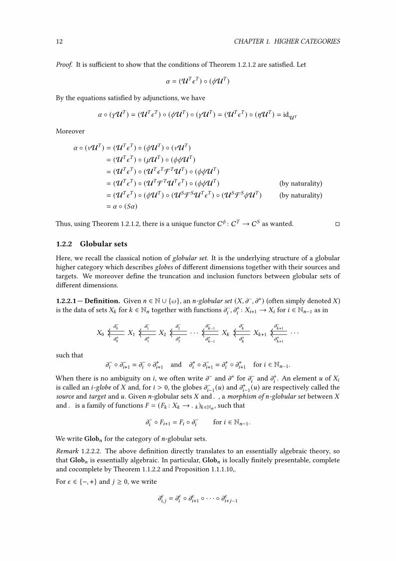
12 CHAPTER 1. HIGHER CATEGORIES

Proof. It is su�cient to show that the conditions of Theorem 1.2.1.2 are satis�ed. Let

U = (U)n) ) ◦ (qU) )

By the equations satis�ed by adjunctions, we have

U ◦ (WU) ) = (U)n) ) ◦ (qU) ) ◦ (WU) ) = (U)n) ) ◦ ([U) ) = idU)

Moreover

U ◦ (aU) ) = (U)n) ) ◦ (qU) ) ◦ (aU) )= (U)n) ) ◦ (`U) ) ◦ (qqU) )= (U)n) ) ◦ (U)n)F)U) ) ◦ (qqU) )= (U)n) ) ◦ (U)F)U)n) ) ◦ (qqU) ) (by naturality)= (U)n) ) ◦ (qU) ) ◦ (U(F (U)n) ) ◦ (U(F (qU) ) (by naturality)= U ◦ ((U)

Thus, using Theorem 1.2.1.2, there is a unique functor Cq : C) → C( as wanted. �

1.2.2 Globular sets

Here, we recall the classical notion of globular set. It is the underlying structure of a globularhigher category which describes globes of di�erent dimensions together with their sources andtargets. We moreover de�ne the truncation and inclusion functors between globular sets ofdi�erent dimensions.

1.2.2.1 — De�nition. Given = ∈ N ∪ {l}, an =-globular set (-, m−, m+) (often simply denoted - )is the data of sets -: for : ∈ N= together with functions m−8 , m

+8 : -8+1 → -8 for 8 ∈ N=−1 as in

-0 -1 -2 · · · -: -:+1 · · ·m−0

m+0

m−1

m+1

m−2

m+2

m−:−1

m+:−1

m−:

m+:

m−:+1

m+:+1

such thatm−8 ◦ m−8+1 = m−8 ◦ m+8+1 and m+8 ◦ m−8+1 = m+8 ◦ m+8+1 for 8 ∈ N=−1.

When there is no ambiguity on 8 , we often write m− and m+ for m−8 and m+8 . An element D of -8is called an 8-globe of - and, for 8 > 0, the globes m−8−1(D) and m+8−1(D) are respectively called thesource and target and D. Given =-globular sets - and . , a morphism of =-globular set between -and . is a family of functions � = (�: : -: → .: ):∈N= , such that

m−8 ◦ �8+1 = �8 ◦ m−8 for 8 ∈ N=−1.

We write Glob= for the category of =-globular sets.

Remark 1.2.2.2. The above de�nition directly translates to an essentially algebraic theory, sothat Glob= is essentially algebraic. In particular, Glob= is locally �nitely presentable, completeand cocomplete by Theorem 1.1.2.2 and Proposition 1.1.1.10,.

For n ∈ {−, +} and 9 ≥ 0, we write

mn8, 9 = mn8 ◦ mn8+1 ◦ · · · ◦ mn8+9−1

1.2. HIGHER CATEGORIES AS GLOBULAR ALGEBRAS 13

for the iterated source (when n = −) and target (when n = +) operations. We generally omitthe index 9 when there is no ambiguity and simply write mn8 (D) for mn8, 9 (D). Given 8, :, ; ∈ N=with 8 < min(:, ;), we write -: ×8 -; for the pullback

-: ×8 -; -;

-: -8

m−8

m+8

.

Given ? ≥ 2 and :1, . . . , :? ∈ N= , a sequence of globes D1 ∈ -:1, . . . , D? ∈ -:? is said 8-com-posable for some 8 < min(:1, . . . , :?), when m+8 (D 9 ) = m−8 (D 9+1) for 9 ∈ N∗?−1. Given : ∈ N=and D, E ∈ -: , D and E are said parallel when : = 0 or mn

:−1(D) = mn:−1(E) for n ∈ {−, +}. To remove

the side condition : = 0, we use the convention that -−1 is the set {∗} and that m−−1, m+−1 are the

unique function -0 → -−1.For D ∈ -8+1, we sometimes write D : E → F to indicate that m−8 (D) = E and m+8 (D) = F . In

low dimension, we use =-arrows such as⇒,V, , etc. to indicate the sources and the targets of=-globes in several dimensions. For example, given a 2-globular set - and q ∈ - , we sometimeswrite q : 5 ⇒ 6 : G → ~ to indicate that

q ∈ -2, m−1 (q) = 5 , m+1 (q) = 6, m−0 (q) = G and m+0 (q) = ~.

We also use these arrows in graphical representations to picture the elements of a globular set - .For example, given an =-globular set - with = ≥ 2, the drawing

G ~ I

5

6

ℎ

⇓q

⇓k: (1.1)

�gures two 2-cells q,k ∈ -2, four 1-cells 5 , 6, ℎ, : ∈ -1 and three 0-cells G,~, I ∈ -0 such that

m−1 (q) = 5 , m+1 (q) = m−1 (k ) = 6, m+1 (k ) = ℎ,m−0 (5 ) = m−0 (6) = m−0 (ℎ) = G, m+0 (5 ) = m+0 (6) = m+0 (ℎ) = m−0 (:) = ~, m+0 (:) = I.

1.2.2.3 — Truncation and inclusion functors. Given < ∈ N= and - ∈ Glob= , we denoteby -≤< the<-truncation of - , i.e., the<-globular set obtained from - by removing the 8-globesfor 8 ∈ N= with 8 > <. This operation extends to a functor

(−)Glob≤<,= : Glob= → Glob<

often denoted (−)Glob≤< when there is no ambiguity. This functor admits a left adjoint

(−)Glob↑=,< : Glob< → Glob=

often denoted (−)Glob↑= when there is no ambiguity, and which maps an<-globular set - to the

=-globular set -↑= , called =-inclusion of - , and which is de�ned by (-↑=)≤< = - and (-↑=)8 = ∅for 8 ∈ N= with 8 > <. The unit of the adjunction (−)Glob

↑= a (−)Glob≤< is the identity and the counit

is the natural transformation denoted i<,= , or simply i< when there is no ambiguity, which isgiven by the family of canonical morphisms

i<- : (-≤<)↑= → -

14 CHAPTER 1. HIGHER CATEGORIES

for - ∈ Glob= . The functor (−)Glob≤<,= also admits a right adjoint

(−)Glob⇑<,= : Glob< → Glob=

denoted (−)Glob⇑< when there is no ambiguity, and which maps an<-globular set to the =-globular

set -⇑= de�ned by (-⇑=)≤< = - , and, for 8 ∈ N= with 8 > <,

(-⇑=)8 = {(D, E) ∈ -< | D and E are parallel}

such that, for (D, E) ∈ (-⇑=)8 ,

m−< ((D, E)) = D and m+< ((D, E)) = Eand

m−9 ((D, E)) = m+9 ((D, E)) = (D, E) for 9 ∈ N8−1.

Note that, since they are left adjoints, the functors (−)Glob↑=,< and (−)Glob

≤<,= preserves colimits.

1.2.3 Globular algebras

We now introduce categories of globular algebras, i.e., the Eilenberg-Moore categories inducedby monads on globular sets, as were �rst introduced by Batanin in [Bat98a]. We moreover giveseveral additional constructions and properties on these objects.

1.2.3.1 — De�nition. Let = ∈ N∪{l} and (), [, `) be a �nitary monad on Glob= . We write Alg=for the category of ) -algebras Glob)= and

U= : Alg= → Glob= F= : Glob= → Alg=

for the induced left and right adjoints, that were denotedU) and F) in Section 1.2.1. Explicitly,given (-,ℎ) ∈ Alg= , the image of (-,ℎ) by U= is - and, given . ∈ Glob= , F=. is the free) -algebra

()., `. : )). → ). ) .Given : ∈ N= , there is a monad (): , [: , `: ) on Glob: de�ned from (), [, `) by

): = (−)Glob≤: ) (−)Glob

↑=

and such that [: : idGlob: → ): is the composite

idGlob: (−)Glob≤: (−)

Glob↑= ):

(−)Glob≤: [ (−)Glob

↑=

i.e., [:-= ([-↑= )≤: for - ∈ Glob: , and such that `: : ):): → ): is the composite

):): (−)Glob≤: )) (−)Glob

↑= ):(−)Glob≤: ) i: ) (−)Glob

↑= (−)Glob≤: ` (−)Glob

↑= .

The axioms of monads are easily veri�ed for (): , [: , `: ) using the fact that (), [, `) is a monad.So, for : ∈ N= , there is a category of algebra Glob)

:

:, that we denote Alg: , and canonical functors

U: : Alg: → Glob: F: : Glob: → Alg:

de�ned like U= and F= above. The objects of Alg: are called :-categories. Moreover, given a:-category � = (-,ℎ), the elements of -8 are called the 8-cells of � for 8 ∈ N: . We can alreadyderive several properties of the categories Alg: :

1.2. HIGHER CATEGORIES AS GLOBULAR ALGEBRAS 15

Proposition 1.2.3.2. For : ∈ N∪{=}, the categoryAlg: is locally �nitely presentable. In particular,it is complete and cocomplete. Moreover, the functorU: preserves and creates directed colimits, andcreates limits.

Proof. The category Alg: is locally �nitely presentable as a consequence of Proposition 1.1.1.12since Glob: is locally �nitely presentable by Remark 1.2.2.2. The functorU: preserves directedcolimits by Proposition 1.1.1.12. Moreover, since U: re�ects isomorphisms and Alg: is cocom-plete,U: creates directed colimits. Finally, it is well-known that the forgetful functor associatedto an Eilenberg-Moore category creates limits (see [Bor94b, Proposition 4.3.1] for example). �

We can usually derive monads from equational de�nitions of higher categories as illustrated bythe following examples.Example 1.2.3.3. Since 1-globular sets are graphs, the �nitary forgetful functorCat→ Gph de�nedin Example 1.1.2.10 induces a �nitary monad (), [, `) on Glob1. This monad maps a 1-globularset� seen as a graph to the underlying 1-globular set of the category of paths on� . Using Beck’smonadicity theorem (Theorem 1.4.1.6), one can verify that the functor Cat→ Gph is monadic, sothat Alg1 ' Cat. Moreover, the monad () 0, [0, `0) is essentially the identity monad on Glob0, andthus Alg0 ' Set. More generally, we will see in Section 1.4.1 that the monads of strict :-categoriesfor : ∈ N are derived from the monad of strict l-categories.Example 1.2.3.4. We de�ne a notion of weird 2-category as follows: a weird 2-category is a 2-glo-bular set � equipped with an operation

∗ : �2 ×�2 → �0.

Note that we do not require the composability of the arguments of ∗, and we do not enforceany axiom on ∗. A morphism between two weird 2-categories is then a morphism between theunderlying 2-globular sets that is compatible with ∗. The category Weird of weird 2-categoriesand their morphisms is essentially algebraic, and the functor which maps a weird 2-categoryto its underlying 2-globular set is induced by an essentially algebraic theory morphism, so thatit is a right adjoint and �nitary by Theorem 1.1.2.7. From the adjunction, we derive a �nitarymonad (), [, `) on Glob2, and, given - ∈ Glob2, we have that

()- )0 ' -0 t (-2 × -2) ()- )1 ' -1 ()- )2 ' -2

so that, for Alg2 derived from the monad ) , Alg2 ' Weird. Moreover, the monads () 0, [0, `0)and () 1, [1, `1) are essentially the identity monads on Glob0 and Glob1 respectively, so that theassociated notions of weird 0- and 1-categories are simply 0- and 1-globular sets.The last example moreover illustrates the unusual operations that notions of higher categoriesde�ned in the setting of Batanin can have. It is also an example of a monad on globular sets whichis not truncable (c.f. Example 1.2.4.3).Remark 1.2.3.5. In the above de�nition, we require that the monad (), [, `) is �nitary in orderto prove later the existence of several free constructions on the :-categories. This is not toorestrictive, since it includes all the monads of algebraic globular higher categories that haveoperations with �nite arities, i.e., most theories of algebraic globular higher categories.

1.2.3.6 — Truncation and inclusion functors. We now introduce truncation and inclusionfunctors between the categories Alg: together with some of their properties. Let = ∈ N ∪ {l}and (), [, `) be a �nitary monad on Glob= . Given :, ; ∈ N= ∪ {=} with : < ; and a ) ; -algebra

(-,ℎ : ) ;- → - ),

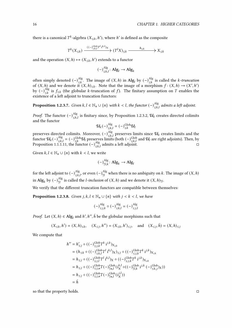
16 CHAPTER 1. HIGHER CATEGORIES

there is a canonical ): -algebra (-≤: , ℎ′), where ℎ′ is de�ned as the composite

): (-≤: ) () ;- )≤: -≤:( (−)Glob

≤:,;); i:,; )- ℎ≤:

and the operation (-,ℎ) ↦→ (-≤: , ℎ′) extends to a functor

(−)Alg≤:,; : Alg; → Alg:

often simply denoted (−)Alg≤: . The image of (-,ℎ) in Alg; by (−)Alg

≤: is called the :-truncationof (-,ℎ) and we denote it (-,ℎ)≤: . Note that the image of a morphism 5 : (-,ℎ) → (- ′, ℎ′)by (−)Alg

≤: is 5≤: (the globular :-truncation of 5 ). The �nitary assumption on ) enables theexistence of a left adjoint to truncation functors:

Proposition 1.2.3.7. Given :, ; ∈ N= ∪ {=} with : < ; , the functor (−)Alg≤:,; admits a left adjoint.

Proof. The functor (−)Alg≤:,; is �nitary since, by Proposition 1.2.3.2, U: creates directed colimits

and the functorU: (−)Alg

≤:,; = (−)Glob≤: U;

preserves directed colimits. Moreover, (−)Alg≤:,; preserves limits since U: creates limits and the

functorU: (−)Alg≤:,; = (−)

Glob≤: U; preserves limits (both (−)Glob

≤:,; andU; are right adjoints). Then, byProposition 1.1.1.11, the functor (−)Alg

≤:,; admits a left adjoint. �

Given :, ; ∈ N= ∪ {=} with : < ; , we write

(−)Alg↑;,: : Alg: → Alg;

for the left adjoint to (−)Alg≤:,; , or even (−)Alg

↑; when there is no ambiguity on : . The image of (-,ℎ)in Alg: by (−)Alg

↑; is called the ;-inclusion of (-,ℎ) and we denote it (-,ℎ)↑; .We verify that the di�erent truncation functors are compatible between themselves:

Proposition 1.2.3.8. Given 9, :, ; ∈ N= ∪ {=} with 9 < : < ; , we have

(−)Alg≤ 9,: ◦ (−)

Alg≤:,; = (−)

Alg≤ 9,;

Proof. Let (-,ℎ) ∈ Alg; and ℎ′, ℎ′′, ℎ be the globular morphisms such that

(-≤: , ℎ′) = (-,ℎ)≤: , (-≤ 9 , ℎ′′) = (-≤: , ℎ′)≤ 9 , and (-≤ 9 , ℎ) = (-,ℎ)≤ 9

We compute that

ℎ′′ = ℎ′≤ 9 ◦ ((−)Glob≤ 9,:)

: i9,: )-≤:= (ℎ≤: ◦ ((−)Glob

≤:,; ); i:,; )- )≤ 9 ◦ ((−)Glob

≤ 9,:): i9,: )-≤:

= ℎ≤ 9 ◦ ((−)Glob≤ 9,; )

; i:,; )- ◦ ((−)Glob≤ 9,:)

: i9,: )-≤:= ℎ≤ 9 ◦ ((−)Glob

≤ 9,=) (−)Glob↑=,; (i

:,;

-◦((−)Glob

↑;,: i9,: (−)Glob≤:,9 )- ))

= ℎ≤ 9 ◦ ((−)Glob≤ 9,=) (−)Glob

↑=,; (i9,;

-))

= ℎ

so that the property holds. �

1.2. HIGHER CATEGORIES AS GLOBULAR ALGEBRAS 17

1.2.3.9 — Alg8 as a limit. Let (), [, `) be a �nitary monad on Globl . The purpose of thisparagraph is to characterize Algl as a limit on the categories Alg: for : ∈ N using the truncationfunctors (−)Alg

≤: . Before showing this property, we need to recall the notion of co�nal functor.First, given a category � , we de�ne a relation ∼� on the objects on � as the smallest equivalencerelation such that, for every 5 : G → ~ ∈ � , we have G ∼� ~. The category� is then said connectedwhen G ∼� ~ for all G,~ ∈ �0. A functor � : � → � between two categories � and � is co�nal when,for each 8 ∈ �0, the arrow category 8 ↓ � is connected. The interesting fact about co�nal functorsis that they witness that two diagrams have the same colimit:

Proposition 1.2.3.10. Let � : � → � be a co�nal functor between two categories � and � , 3 : � → �

be a functor into a category � and ? : 3 ⇒ Δ; be a cocone on 3 of vertex ; ∈ �0 (where Δ; is theconstant functor � → � of value ;). Then, ? is a colimit cocone on 3 if and only if ?� is a colimitcocone on 3 ◦ � .

Proof. See [Mac13, Section IX.3] or [KS06, Section 2.5]. �

The co�nal functors between two directed categories are easily characterized:

Proposition 1.2.3.11. Let � : � → � be a functor between two directed categories � and � . Then, �is co�nal if and only if, for each 9 ∈ � , there exists 8 ∈ � and a morphism 9 → � (8) ∈ � .

Proof. The implication is clear. Conversely, suppose that for each 9 ∈ � , there exists 8 ∈ � and amorphism 9 → � (8) ∈ � . Then, given 9 ∈ � , the category 9 ↓ � is not empty. Moreover, given twomorphisms 51 : : 9 → � (81) and 52 : 9 → � (82) in � for some 81, 82 ∈ � , since � is directed, thereexist morphisms 61 : 81 → 8 and 62 : 82 → 8 for some 8 ∈ � , that induce morphisms

61 : (81, 51) → (8, 61 ◦ 51) and 62 : (82, 52) → (8, 62 ◦ 52)

in 9 ↓ � . Since � is directed, we have 61 ◦ 51 = 62 ◦ 52. Thus, 9 ↓ � is connected. Hence, � isco�nal. �

We can now characterize Algl as a limit:

Proposition 1.2.3.12. ((−)Alg≤: : Algl → Alg: ):∈N is a limit cone in CAT on the diagram

Alg0 Alg1 Alg2 · · · Alg: Alg:+1 · · ·(−)Alg≤0 (−)Alg

≤1 (−)Alg≤2 (−)Alg

≤:−1 (−)Alg≤: (−)Alg

≤:+1

Proof. Let �: = (-: , 6: : ):-: → - ) ∈ Alg: for : ∈ N be such that �:+1≤: = �: . Then, inparticular, we have -:+1≤: = -: , so that there exists - ∈ Globl such that -: = -≤: for : ∈ N.Let ': be the functor

': = (−)Glob↑l (−)

Glob≤: : Globl → Globl

and ) ;,: be the functor) ;,: = ';)': : Globl → Globl

and j: be the natural transformation

j: = (−)Glob↑l i:,:+1 (−)Glob

≤:+1 : ': ⇒ ':+1

for :, ; ∈ N. Note that, for all . ∈ Globl , (i:,l.

: ':. → . ):∈N is a colimit cocone in Globl onthe diagram

'0. '1. · · · ':. ':+1. · · ·j0.

j1.

j:−1.

j:.

j:+1.

18 CHAPTER 1. HIGHER CATEGORIES

Since ) is �nitary, (() i:,l )- : ) (-≤: )↑l → )- ):∈N is a colimit cocone on the diagram

)'0- )'1- · · · )':- )':+1- · · ·() j0)- () j1)- () j:−1)- () j: )- () j:+1)-

By commutation of colimits, ((i;,l ) i:,l )- : ) ;,:- → )- ):,; ∈N is a colimit cocone of the griddiagram

......

· · · ) ;+1,:- ) ;+1,:+1- · · ·

· · · ) ;,: ) ;,:+1 · · ·

......

(';+1) j:−1)- (';+1) j: )-

(j;+1)': )-

(';+1) j:+1)-

(j;+1)':+1)-

(';) j:−1)-

(j; )': )-

(';) j: )- (';) j:+1)-

(j; )':+1)-

(j;−1)': )- (j;−1)':+1)-

Note that the diagonal functor Δ : (N, ≤) → (N × N, ≤ × ≤) is co�nal by Proposition 1.2.3.11, sothat, by Proposition 1.2.3.10, the cocone ((i:,l ) i:,l )- : ):,:- → )- ):∈N is a colimit cocone onthe diagram

) 0,0- · · · ):,:- ):+1,:+1- · · ·(j0) j0)- (j:−1) j:−1)- (j: ) j: )- (j:+1) j:+1)- (1.2)

where ):,:- is exactly ():-: )↑l for : ∈ N and, by the de�nition of (−)Alg≤: , we have

6: = 6:+1≤: ◦ ((−)Glob≤: ) j: )-

so that

j:- ◦6:↑l = ((−)Glob

↑l i:,:+1 (−)Glob≤:+1)- ◦ (6

:+1≤: )↑l ◦ ('

:) j: )-= ((−)Glob

↑l i:,:+1)-:+1 ◦ (6:+1≤: )↑l ◦ (':) j: )-

= 6:+1↑l ◦ ((−)Glob↑l i:,:+1)):+1-:+1 ◦ (':) j: )- (by naturality of (−)Glob

↑l i:,:+1)

= 6:+1↑l ◦ (j: )':+1)- ◦ (':) j: )-

= 6:+1↑l ◦ (j: ) j: )- .

Thus, we obtain a diagram

() 0(-≤0))↑l · · · (): (-≤: ))↑l ():+1(-≤:+1))↑l · · ·

(-≤0)↑l · · · (-≤: )↑l (-≤:+1)↑l · · ·

(j0) j0)-

60↑l

(j:−1) j:−1)- (j: ) j: )-

6:↑l

(j:+1) j:+1)-

6:+1↑lj0-

j:−1-

j:-

j:+1-

where each square commutes, and it induces a morphism 6 : )- → - ∈ Globl . By a similarargument as above, we have a colimit cocone

((i:,l ) i:,l ) i:,l )- : ():):-: )↑l → ))- ):∈N

1.2. HIGHER CATEGORIES AS GLOBULAR ALGEBRAS 19

on a diagram analogous to (1.2). We compute that, for : ∈ N,

6 ◦ `- ◦ (i:,l ) i:,l ) i:,l )-= 6 ◦ `- ◦ (i:,l )) i:,l )- ◦ (':) i:,l )': )- (by naturality)

= 6 ◦ (i:,l ) i:,l )- ◦ (':`': )- ◦ (':) i:,l )': )- (by naturality)

= i:,l-◦6:↑l ◦ ((−)

Glob↑l `: (−)Glob

≤: )- (by de�nition of 6 and `: )

= i:,l-◦6:↑l ◦ ((−)

Glob↑l `: )-≤:

= i:,l-◦(6: ◦ `:-≤: )↑l

= i:,l-◦(6: ◦): (6: ))↑l (since (-: , 6: ) is an algebra)

= 6 ◦ (i:,l ) i:,l )- ◦ (): (6: ))↑l (by de�nition of 6)

= 6 ◦ (i:,l ) )- ◦ ':) (i:,l- ◦6:↑l )

= 6 ◦ (i:,l ) )- ◦ ':) (6 ◦ (i:,l ) i:,l )- ) (by de�nition of 6)

= 6 ◦ (i:,l ) )- ◦ ':) (6) ◦ (':) i:,l ) i:,l )-= 6 ◦) (6) ◦ (i:,l ) )- ◦ (':) i:,l ) i:,l )- (by naturality)

= 6 ◦) (6) ◦ (i:,l ) i:,l ) i:,l )-

so that 6 ◦ `- = 6 ◦) (6). Moreover, for : ∈ N, we have

6 ◦ [- ◦ i:,l-

= 6 ◦ [- ◦ i:,l-◦(': i:,l )- (since (': i:,l )- = id

':-)

= 6 ◦ [- ◦ (i:,l i:,l )-= 6 ◦ (i:,l ) i:,l )- ◦ (':[': )- (by naturality)

= i:,l ◦6:↑l ◦ ((−)Glob↑l [: (−)Glob

≤: )-= i:,l ◦6:↑l ◦ ((−)

Glob↑l [: )-:

= i:,l ◦(6: ◦ [:-:)↑l

= i:,l (since (-: , 6: ) is an algebra)

thus, since (i:,l : ':- → - ): is a colimit cocone, we have 6 ◦ [- = id- . Hence, (-,6) ∈ Algl .For : ∈ N, let (-: , 6: : ): (-≤: ) → -≤: ) be the image of (-,6) by (−)Alg

≤: . We have

i:,l-◦6:↑l = i:,l

-◦': (6) ◦ (':) i:,l )- (by de�nition of (−)Alg

≤: )

= 6 ◦ i:,l)-◦(':) i:,l )- (by naturality of i:,l )

= 6 ◦ (i:,l ) i:,l )-= i:,l ◦6:↑l (by de�nition of 6)

thus, since i:,l is a monomorphism and (−)Glob↑l is faithful, we have 6: = 6: . Moreover, given an

algebra (-, 6) ∈ Algl such that (-, 6)≤: = (-: , 6: ) for every : ∈ N, we have

6 ◦ (i:,l ) i:,l )- = 6 ◦ i:,l)-◦(':) i:,l )-

= i:,l-◦': (6) ◦ (':) i:,l )- (by naturality of i:,l

-)

= i:,l-◦6:↑l (by de�nition of (−)Alg

≤: )

= 6 ◦ (i:,l ) i:,l )-

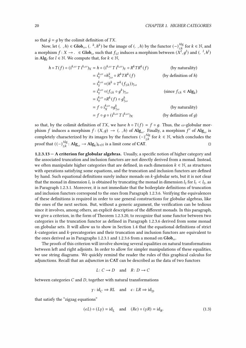
20 CHAPTER 1. HIGHER CATEGORIES

so that 6 = 6 by the colimit de�nition of )- .Now, let (.,ℎ) ∈ Globl , (.: , ℎ: ) be the image of (.,ℎ) by the functor (−)Alg

≤: for : ∈ N, anda morphism 5 : - → . ∈ Globl such that 5≤; induces a morphism between (- ; , 6; ) and (. ; , ℎ; )in Alg; for ; ∈ N. We compute that, for : ∈ N,

ℎ ◦) (5 ) ◦ (i:,l ) i:,l )- = ℎ ◦ (i:,l ) i:,l ). ◦ ':)': (5 ) (by naturality)

= i:,l.◦ℎ:↑l ◦ '

:)': (5 ) (by de�nition of ℎ)

= i:,l.◦(ℎ: ◦): (5≤: ))↑l

= i:,l.◦(5≤: ◦ 6: )↑l (since 5≤: ∈ Alg: )

= i:,l.◦': (5 ) ◦ 6:↑l

= 5 ◦ i:,l-◦6:↑l (by naturality)

= 5 ◦ 6 ◦ (i:,l ) i:,l )- (by de�nition of 6)

so that, by the colimit de�nition of )- , we have ℎ ◦ ) (5 ) = 5 ◦ 6. Thus, the l-globular mor-phism 5 induces a morphism 5 : (-,6) → (.,ℎ) of Algl . Finally, a morphism 5 ′ of Algl iscompletely characterized by its images by the functors (−)Alg

≤: for : ∈ N, which concludes theproof that ((−)Alg

≤: : Algl → Alg: ):∈N is a limit cone of CAT. �

1.2.3.13 — A criterion for globular algebras. Usually, a speci�c notion of higher category andthe associated truncation and inclusion functors are not directly derived from a monad. Instead,we often manipulate higher categories that are de�ned, in each dimension : ∈ N, as structureswith operations satisfying some equations, and the truncation and inclusion functors are de�nedby hand. Such equational de�nitions surely induce monads on :-globular sets, but it is not clearthat the monad in dimension ;1 is obtained by truncating the monad in dimension ;2 for ;1 < ;2, asin Paragraph 1.2.3.1. Moreover, it is not immediate that the boilerplate de�nitions of truncationand inclusion functors correspond to the ones from Paragraph 1.2.3.6. Verifying the equivalencesof these de�nitions is required in order to use general constructions for globular algebras, likethe ones of the next section. But, without a generic argument, the veri�cation can be tedioussince it involves, among others, an explicit description of the di�erent monads. In this paragraph,we give a criterion, in the form of Theorem 1.2.3.20, to recognize that some functor between twocategories is the truncation functor as de�ned in Paragraph 1.2.3.6 derived from some monadon globular sets. It will allow us to show in Section 1.4 that the equational de�nitions of strict:-categories and :-precategories and their truncation and inclusion functors are equivalent tothe ones derived as in Paragraphs 1.2.3.1 and 1.2.3.6 from a monad on Globl .

The proofs of this criterion will involve showing several equalities on natural transformationsbetween left and right adjoints. In order to allow for simpler manipulations of these equalities,we use string diagrams. We quickly remind the reader the rules of this graphical calculus foradjunctions. Recall that an adjunction in CAT can be described as the data of two functors

! : � → � and ' : � → �

between categories � and � , together with natural transformations

W : id� ⇒ '! and n : !' ⇒ id�

that satisfy the “zigzag equations”

(n!) ◦ (!W) = id! and ('n) ◦ (W') = id' . (1.3)

1.2. HIGHER CATEGORIES AS GLOBULAR ALGEBRAS 21

One can represent the above situation using string diagrams as follows: the natural transforma-tions W and n can be pictured as

' !

Wand

! '

n

and the zigzag equations can be pictured by

!

!

W

n

=

!

!

and

'

'

W

n

=

'

'

.

Note that the above equations generate a congruence: they apply as well when both sides appear assubdiagrams of a bigger string diagram. Using this language, we graphically show the elementaryproperty that an isomorphism between two left adjoints induces an isomorphism between thetwo right adjoints (and vice versa):

Proposition 1.2.3.14. Let

! a ' : � → � and !′ a '′ : � → �

be two adjunctions with respective unit-counit pairs (W, n) and (W ′, n ′), and

\ : ! ⇒ !′ and \ : '′⇒ '

be two natural transformations such that \ = (n!′) ◦ (!\!′) ◦ (!W ′), i.e., graphically:

\

!

!′

= \! !′

W ′

n

.

Then, \ is an isomorphism if and only if \ is an isomorphism.

Proof. Suppose �rst that \ is an isomorphism. Note that, by the zigzag equations satis�ed by (W, n)and (W ′, n ′), we have

\' '′

W

n ′

= \

'′

'

.

22 CHAPTER 1. HIGHER CATEGORIES

By the same zigzag equations, one then easily veri�es that the morphism depicted by the followingstring diagram is an inverse to \ :

\−1'′ '

W ′

n

.

Conversely, suppose that \ is an isomorphism. Then, by the zigzag equations, one easily veri�esthat the diagram

\−1!′ !

W

n ′

de�nes an inverse of \ , which concludes the proof. �

Moreover, we recall how to derive an adjunction from the composition of two adjunctions, usingthe graphical language:

Proposition 1.2.3.15. Given two adjunctions !1 a '1 : �1 → �2 and !2 a '2 : �2 → �3 withunit-counit pairs (W1, n1) and (W2, n2) respectively, there is a canonical adjunction !1!2 a '2'1 whoseunit and counit are respectively

('2W1!2) ◦ W2 and n1 ◦ (!1n2'1)

that can be represented by

'2 '1 !1 !2

W1

W2

and

!1 !2 '2 '1

n1

n2 .

Proof. Using the zigzag equations satis�ed by (W1, n1) and (W2, n2), we easily verify that

'2 '1 !1 !2 '2 '1

W1

W2

n1

n2

= '2 '1

1.2. HIGHER CATEGORIES AS GLOBULAR ALGEBRAS 23

and

!1 !2 '2 '1 !1 !2

W1

W2

n1

n2

= !1 !2

so that ('2W1!2) ◦ W2 and n1 ◦ (!1n2'1) equip the functors !1!2 and '2'1 with a structure of anadjunction !1!2 a '2'1 : �1 → �3. �

Note that Proposition 1.2.3.15 generalizes to compositions of sequences of adjunctions

!1 a '1 : �1 → �2, . . . , !: a ': : �: → �:+1

for every : ∈ N∗. We now show several technical lemmas that we will use in the proof ofTheorem 1.2.3.20 below.

Lemma 1.2.3.16. Let the (not necessarily commutative) diagram of functors in CAT

�

�

� ′

'

*

!

!′'′

�

where ! a ', !′ a '′ and � a * are adjunctions such that '′* = ', and write ((,W, a) and (( ′, W ′, a ′)for the monads associated to ! a ' and !′ a '′ respectively. Then, the unit of the adjunction � a *induces a morphism of monads q : ( ′⇒ ( such that the following diagram commutes

� �(

� ′ �(′

�

* �q

� ′

where � and � ′ are the comparison functors associated to the adjunctions ! a ' and !′ a '′.

Proof. Let (U, X), (V, n), (V ′, n ′) be the unit-counit pairs of the adjunctions � a * , ! a ', and !′ a '′respectively. Note that V = W and V ′ = W ′. Since '′* = ', the natural transformation \ : �!′⇒ !

de�ned as the composite\ = (X!) ◦ (�n ′*!) ◦ (�!′W)

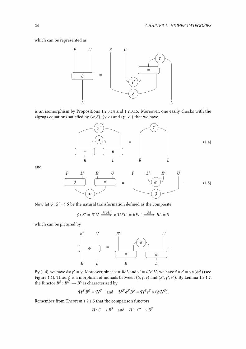
24 CHAPTER 1. HIGHER CATEGORIES

which can be represented as

� !′

!

\ =

� !′

!

W

n ′

X

=

is an isomorphism by Propositions 1.2.3.14 and 1.2.3.15. Moreover, one easily checks with thezigzags equations satis�ed by (U, X), (W, n) and (W ′, n ′) that we have

W ′

U

= \

' !

=

W

' !

(1.4)

and� !′ '′ *

\ =

n

=

� !′ '′ *

n ′

X

. (1.5)

Now let q : ( ′⇒ ( be the natural transformation de�ned as the composite

q : ( ′ = '′!′ '′*�!′ = '�!′ '! = ('′U!′ '\

which can be pictured by

'′ !′

' !

q =

'′ !′

U

= \

' !

.

By (1.4), we have q ◦W ′ = W . Moreover, since a = 'n! and a ′ = '′n ′!′, we have q ◦a ′ = a ◦ (qq) (seeFigure 1.1). Thus, q is a morphism of monads between ((,W, a) and (( ′, W ′, a ′). By Lemma 1.2.1.7,the functor �q : �(′ → �( is characterized by

U(′�q = U( and U(′n(′�q = U(n( ◦ (qU( ).

Remember from Theorem 1.2.1.5 that the comparison functors

� : � → �( and � ′ : � ′→ �(′

1.2. HIGHER CATEGORIES AS GLOBULAR ALGEBRAS 25

'′ !′ '′ !′

U

= \

n ′

' !

=

'′ !′ '′ !′

U

=

U

\n ′

X

' !

(by zigzag equations)

=

'′ !′ '′ !′

U

= \

U

= \

n

' !

(by (1.5))

Figure 1.1 – Proof that q ◦ a ′ = a ◦ (qq)

26 CHAPTER 1. HIGHER CATEGORIES

'′ !′ '

U

= \

n

'

=

'′ !′ '

=

U

=

n ′

X'

(by (1.5))

=

'′ !′ '

=

=

n ′

'

(by zigzag equations)

Figure 1.2 – Proof that ('n) ◦ (q') = '′n ′*

are the unique functors such that

U(� = ' U(′� ′ = '′

U(n(� = 'n U(′n(′� ′ = '′n ′.

Thus,U(′�q� = U(� = ' = '′* = U(′� ′* .

Moreover, we have ('n) ◦ (q') = '′n ′* (see Figure 1.2), so that

U(′n(′�q� = (U(n(� ) ◦ (qU(� ) = ('n) ◦ (q') = '′n ′* = U(′n(

′� ′* .

We conclude by Theorem 1.2.1.2 that �q� = � ′* . �

Lemma 1.2.3.17. Let �1 a *1 and I ′ a T ′ be adjunctions as in

�1 �1 �2*1 T′

�1 I′

1.2. HIGHER CATEGORIES AS GLOBULAR ALGEBRAS 27

and write()1, [1, `1) and (( ′, W ′, a ′)

for the monads associated to the adjunctions �1 a *1 and �1I ′ a T ′*1. The comparison functor

T ′′ : �)11 → �(

′2

induced by the adjunction F)1I ′ a T ′U)1 : �)11 → �2 makes the following diagram commutes

�1 �)11 �1

�(′

2 �2

�1

� ′

U)1

T′′ T′

U(′

where �1 and � ′ are the comparison functors induced by the adjunctions �1 a *1 and �1I ′ a T ′*1respectively.

Proof. By the de�nition of T ′′ (given in Theorem 1.2.1.5), the right square commutes. In order toshow that the left triangle commutes, we use the characterization of functors � → �(

′2 given by

Theorem 1.2.1.2. First, we compute that

U(′� ′ = T ′*1 = T ′U)1�1 = U(′T ′′�1.

Moreover, writting n1 and n ′ for the counit of �1 a *1 and I ′ a T ′ respectively, we have

U(′n(′� ′ = (T ′*1n1) ◦ (T ′)1n

′*1) (by de�nition of � ′ and Proposition 1.2.3.15)= T ′U)1n)1�1 (by de�nition of �1)

= U(′n(′T ′′�1 (by de�nition of T ′′).

Thus T ′′�1 = �′ by Theorem 1.2.1.2. �

Lemma 1.2.3.18. Let a commutative square

�1 �1

�2 �2

*1

T T′

*2

where*1,*2,T ,T ′ are right adjoints with associated left adjoints �1, �2,I,I ′, such that*1,*2 aremonadic and I is fully faithful. Write

()1, [1, `1) ()2, [2, `2) ((,W, a) (( ′, W ′, a ′)

for the monads associated with the adjunctions

�1 a *1 �2 a *2 I�2 a *2T �1I ′ a T ′*1

respectively, and write

�1 : �1 → �)11 and T ′′ : �)1

1 → �(′

2

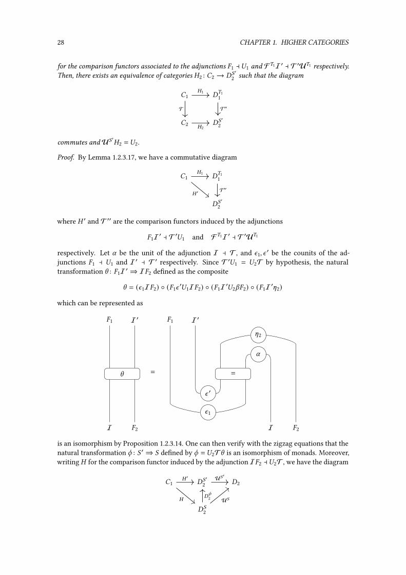
28 CHAPTER 1. HIGHER CATEGORIES

for the comparison functors associated to the adjunctions �1 a *1 and F)1I ′ a T ′U)1 respectively.Then, there exists an equivalence of categories �2 : �2 → �(

′2 such that the diagram

�1 �)11

�2 �(′

2

�1

T T′′

�2

commutes andU(′�2 = *2.

Proof. By Lemma 1.2.3.17, we have a commutative diagram

�1 �)11

�(′

2

�1

� ′T′′

where � ′ and T ′′ are the comparison functors induced by the adjunctions

�1I ′ a T ′*1 and F)1I ′ a T ′U)1

respectively. Let U be the unit of the adjunction I a T , and n1, n′ be the counits of the ad-

junctions �1 a *1 and I ′ a T ′ respectively. Since T ′*1 = *2T by hypothesis, the naturaltransformation \ : �1I ′⇒ I�2 de�ned as the composite

\ = (n1I�2) ◦ (�1n′*1I�2) ◦ (�1I ′*2V�2) ◦ (�1I ′[2)

which can be represented as

�1 I ′

I �2

\ =

�1 I ′

I �2

[2

U

n ′

n1

=

is an isomorphism by Proposition 1.2.3.14. One can then verify with the zigzag equations that thenatural transformation q : ( ′⇒ ( de�ned by q = *2T\ is an isomorphism of monads. Moreover,writing� for the comparison functor induced by the adjunction I�2 a *2T , we have the diagram

�1 �(′

2 �2

�(2

� ′

�

U(′

U(�q

2

1.2. HIGHER CATEGORIES AS GLOBULAR ALGEBRAS 29

where the left triangle commutes by the de�nitions of �,� ′, �q2 and the characterization offunctors �1 → �(2 (c.f. Theorem 1.2.1.2), and the right triangle commutes by Lemma 1.2.1.7.Writingk : )2 ⇒ ( for the morphism of monads induced by the unit of I a T , by Lemmas 1.2.1.7and 1.2.3.16, we have a commutative diagram

�1 �(2 �2

�2 �)22

�

T

U(

�k

2

�2

U)2

where �2 is the comparison functor induced by the adjunction �2 a *2. Since I is supposed fullyfaithful, the unit of I a T is an isomorphism, so that �k2 is an isomorphism. Write �2 for

�2 = �q

2 (�k

2 )−1�2.

From the above commutative diagrams, we deduce that

�1 �)11

�2 �(′

2

�1

T T′′

�2

commutes. Moreover, since *1 and *2 were supposed monadic, �1 and �2 are equivalence ofcategories (and so is �2). By the de�nition of �1 and �2, we haveU)1�1 = *1 andU)2�2 = *2.From the later equality and the above commutative diagrams, we deduce thatU(′�2 = *2. �

Lemma 1.2.3.19. Let :, = ∈ N ∪ {l} with : < = and (), [, `) be a �nitary monad on Glob= . Thecomparison functor associated to the adjunction

F= (−)Glob↑= a (−)Glob

≤: U= : Alg= → Glob:

is (−)Alg≤: : Alg= → Alg: .

Proof. By de�nition of (−)Alg≤: , we have

U: (−)Alg≤: = (−)Glob

≤: U= .

Moreover, given (-,ℎ : )=- → - ) ∈ Alg= , recall that the image of (-,ℎ) by (−)Alg≤: is (-≤: , ℎ′),

whereℎ′ = ℎ≤: ◦ ((−)Glob

≤: ) i:,=)- .

Writting n= for the counit of F= a U= and X for the counit of F= (−)Glob↑= a (−)Glob

≤: U= , we have

ℎ′ = ((−)Glob≤: U=n

=)(-,ℎ) ◦ ((−)Glob≤: U=F= i:,=U=)(-,ℎ) = ((−)Glob

≤: U=X)(-,ℎ) .

Thus, writting n: for the counit of F: a U: , we have

(U:n: (−)Alg≤: )(-,ℎ) = ℎ

′ = ((−)Glob≤: U=X)(-,ℎ)

so that (−)Alg≤: is the comparison functor associated to F= (−)Glob

↑= a (−)Glob≤: U= as a consequence

of Theorem 1.2.1.5. �

30 CHAPTER 1. HIGHER CATEGORIES

We have now enough material to show the following criterion for recognizing that some functorbetween two categories is equivalent to the truncation functor between two categories of globularalgebras as de�ned in Paragraph 1.2.3.6:

Theorem 1.2.3.20. Let :, = ∈ N ∪ {l} with : < =, and a diagram in CAT

� Glob=

� ′ Glob:

*1

T (−)Glob≤:

�1

*2

I

�2

such that (−)Glob≤: *1 = *2T and such that we have adjunctions

�1 a *1 �2 a *2 I a T

where I is fully faithful and *1,*2 are monadic. Write (), [, `) for the monad induced by �1 a *1,and Alg= and Alg: for the globular algebras de�ned from ) , and � : � → Alg= for the comparisonfunctor induced by �1 a *1. Then, there exists an equivalence of categories

� ′ : � ′→ Alg:

making the following diagram commute

� Alg=

� ′ Alg:

�

T (−)Alg≤:

� ′

and such thatU:� ′ = *2.

Remark 1.2.3.21. By its de�nition as comparison functor, � satis�es thatU=� = *1. Since *1 ismonadic, � is moreover an equivalence of categories.

Proof. By Theorem 1.2.1.5, we haveU=� = *1. The last part of the statement is a consequenceof Lemmas 1.2.3.18 and 1.2.3.19. �

In the above theorem, � and � ′ should be thought as categories of =-categories and :-categories,and T as a truncation functor, all de�ned “by hand” outside Batanin’s setting. The theoremthen gives a criterion to know whether these objects are equivalent to the ones de�ned in Para-graphs 1.2.3.1 and 1.2.3.6. In particular, we will use this theorem to show that the equationalde�nitions of strict categories and precategories, and their truncation functors, are equivalent tothe ones given by Batanin’s setting (c.f. Theorems 1.4.2.8 and 1.4.1.10). For now, we illustrate theuse of Theorem 1.2.3.20 on a dummy example:Example 1.2.3.22. Consider the monad (), [, `) on Glob1 de�ned in Example 1.2.3.3. Write U1 forthe monadic functor Cat→ Glob1 de�ned in Example 1.1.2.10 (where we identify the categoryof graphs Gph with the category of 1-globular sets Glob1), and write U0 for the identity functorbetween Set and Glob0, which is monadic too. Consider the canonical functor T : Cat → Setwhich maps a small category� to its underlying set of 0-cells�0. This functor makes the followingdiagram commute:

Cat Glob1

Set Glob0

U1

T (−)Glob≤0

U0

.

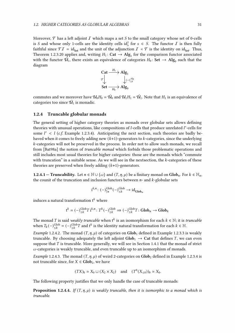
1.2. HIGHER CATEGORIES AS GLOBULAR ALGEBRAS 31

Moreover, T has a left adjoint I which maps a set ( to the small category whose set of 0-cellsis ( and whose only 1-cells are the identity cells id1

B for B ∈ ( . The functor I is then fullyfaithful since TI = idSet and the unit of the adjunction I a T is the identity on idSet. Thus,Theorem 1.2.3.20 applies and, writing �1 : Cat → Alg1 for the comparison functor associatedwith the functor U1, there exists an equivalence of categories �0 : Set → Alg0 such that thediagram

Cat Alg1

Set Alg0

�1

T (−)Alg≤0

�0

commutes and we moreover haveU0�0 = U0 andU1�1 = U1. Note that �1 is an equivalence ofcategories too since U1 is monadic.

1.2.4 Truncable globular monads

The general setting of higher category theories as monads over globular sets allows de�ningtheories with unusual operations, like compositions of ;-cells that produce unrelated ; ′-cells forsome ; ′ < ; (c.f. Example 1.2.3.4). Anticipating the next section, such theories are badly be-haved when it comes to freely adding new (:+1)-generators to :-categories, since the underlying:-categories will not be preserved in the process. In order not to allow such monads, we recallfrom [Bat98a] the notion of truncable monad which forbids those problematic operations andstill includes most usual theories for higher categories: those are the monads which “commutewith truncation” in a suitable sense. As we will see in the nextsection, the :-categories of thesetheories are preserved when freely adding (:+1)-generators.

1.2.4.1 — Truncability. Let = ∈ N∪ {l} and (), [, `) be a �nitary monad on Glob= . For : ∈ N= ,the counit of the truncation and inclusion functors between =- and :-globular sets

i:,= : (−)Glob↑= (−)

Glob≤: → idGlob=

induces a natural transformation t: where

t: = (−)Glob≤: ) i:,= : ): (−)Glob

≤: ⇒ (−)Glob≤: ) : Glob= → Glob:

The monad ) is said weakly truncable when t: is an isomorphism for each : ∈ N; it is truncablewhen ): (−)Glob

≤: = (−)Glob≤: ) and t: is the identity natural transformation for each : ∈ N.

Example 1.2.4.2. The monad (), [, `) of categories on Glob1 de�ned in Example 1.2.3.3 is weaklytruncable. By choosing adequately the left adjoint Glob1 → Cat that de�nes ) , we can evensuppose that ) is truncable. More generally, we will see in Section 1.4.1 that the monad of strictl-categories is weakly truncable, and even truncable up to an isomorphism of monads.

Example 1.2.4.3. The monad (), [, `) of weird 2-categories on Glob2 de�ned in Example 1.2.3.4 isnot truncable since, for - ∈ Glob2, we have

()- )0 ' -0 t (-2 × -2) and () 0(-≤0))0 ' -0.

The following property justi�es that we only handle the case of truncable monads:

Proposition 1.2.4.4. If (), [, `) is weakly truncable, then it is isomorphic to a monad which istruncable.

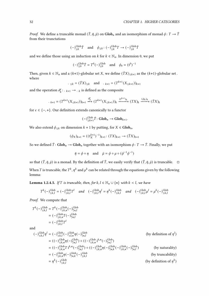
32 CHAPTER 1. HIGHER CATEGORIES

Proof. We de�ne a truncable monad () , [, ¯) on Glob= and an isomorphism of monad q : ) → )

from their trunctations

(−)Glob≤: ) and q≤: : (−)Glob

≤: ) → (−)Glob≤: )

and we de�ne those using an induction on : for : ∈ N= . In dimension 0, we put

(−)Glob≤0 ) = ) 0(−)Glob

≤0 and q0 = (t0)−1

Then, given : ∈ N= and a (:+1)-globular set - , we de�ne ()- )≤:+1 as the (:+1)-globular set .where

.≤: = ()- )≤: and .:+1 = ():+1(-≤:+1)):+1and the operation mn

:: .:+1 → .: is de�ned as the composite

.:+1 = ():+1(-≤:+1)):+1mn:−−→ ():+1(-≤:+1)):

(t:+1):−−−−−→ ()- ):(q: ):−−−−→ ()- ):

for n ∈ {−, +}. Our de�nition extends canonically to a functor

(−)Glob≤:+1) : Glob= → Glob:+1.

We also extend q≤: on dimension : + 1 by putting, for - ∈ Glob= ,

(q- ):+1 = ((t:+1- )−1):+1 : ()- ):+1 → ()- ):+1

So we de�ned ) : Glob= → Glob= together with an isomorphism q : ) → ) . Finally, we put

[ = q ◦ [ and ¯ = q ◦ ` ◦ (q−1q−1)

so that () , [, ¯) is a monad. By the de�nition of ) , we easily verify that () , [, ¯) is truncable. �

When) is truncable, the): , [: and `: can be related through the equations given by the followinglemma:

Lemma 1.2.4.5. If ) is truncable, then, for :, ; ∈ N= ∪ {=} with : < ; , we have

): (−)Glob≤:,; = (−)

Glob≤:,; )

; and (−)Glob≤:,; [

; = [: (−)Glob≤:,; and (−)Glob

≤:,; `; = `: (−)Glob

≤:,;

Proof. We compute that

): (−)Glob≤:,; = )

: (−)Glob≤:,= (−)

Glob↑=,;

= (−)Glob≤:,=) (−)

Glob↑=,;

= (−)Glob≤:,; )

;

and(−)Glob≤:,; [

; = (−)Glob≤:,; (−)

Glob≤;,= [ (−)

Glob↑=,; (by de�nition of [; )

= ((−)Glob≤:,=[ (−)

Glob↑=,; ) ◦ ((−)

Glob≤:,= i:,= (−)Glob

↑=,; )

= ((−)Glob≤:,=) i:,= (−)Glob

↑=,; ) ◦ ((−)Glob≤:,=[ (−)

Glob↑=,: (−)

Glob≤:,= (−)

Glob↑=,; ) (by naturality)

= (−)Glob≤:,=[ (−)

Glob↑=,: (−)

Glob≤:,; (by truncability)

= [: (−)Glob≤:,; (by de�nition of [: )

1.2. HIGHER CATEGORIES AS GLOBULAR ALGEBRAS 33

and(−)Glob≤:,; `

; = ((−)Glob≤:,; (−)

Glob≤;,= ` (−)

Glob↑=,; ) ◦ ((−)

Glob≤:,; (−)

Glob≤;,=) i;,=) (−)Glob

↑=,; ) (by de�nition of `; )

= ((−)Glob≤:,=` (−)

Glob↑=,; ) ◦ ((−)

Glob≤:,; (−)

Glob≤;,=) i;,=) (−)Glob

↑=,; )

= ((−)Glob≤:,=` (−)

Glob↑=,; ) (by truncability)

= ((−)Glob≤:,=` (−)

Glob↑=,; ) ◦ ((−)

Glob≤:,=) i:,=) (−)Glob

↑=,; ) (by truncability)

= ((−)Glob≤:,=` (−)

Glob↑=,; ) ◦ ((−)

Glob≤:,=) i:,=) (−)Glob

↑=,; )

◦ ((−)Glob≤:,=) (−)

Glob↑=,: (−)

Glob≤:,=) i:,= (−)Glob

↑=,; ) (by truncability)

= ((−)Glob≤:,=` (−)

Glob↑=,; ) ◦ ((−)

Glob≤:,=)) i:,= (−)Glob

↑=,; )

◦ ((−)Glob≤:,=) i:,=) (−)Glob

↑=,: (−)Glob≤:,= (−)

Glob↑=,; ) (by naturality)

= ((−)Glob≤:,=) i:,= (−)Glob

↑=,; ) ◦ ((−)Glob≤:,=` (−)

Glob↑=,: (−)

Glob≤:,= (−)

Glob↑=,; )

◦ ((−)Glob≤:,=) i:,=) (−)Glob

↑=,: (−)Glob≤:,= (−)

Glob↑=,; ) (by naturality)

= ((−)Glob≤:,=` (−)

Glob↑=,: (−)

Glob≤:,; ) ◦ ((−)

Glob≤:,=) i:,=) (−)Glob

↑=,: (−)Glob≤:,; ) (by truncability)

= `: (−)Glob≤:,; (by de�nition of `: )

which concludes the proof. �

We now prove several properties of truncable monads regarding truncation of algebras. First, thetruncation of algebras has now a simpler de�nition:

Proposition 1.2.4.6. If ) is truncable, then given :, ; ∈ N= ∪ {=} such that : < ; , and an ;-alge-bra (-,ℎ) ∈ Alg; , we have (-,ℎ)≤: = (-≤: , ℎ≤: ).

Proof. Indeed, since ) is truncable, we have

((−)Glob≤:,; )

; i:,; )- = (): (−)Glob≤:,; i:,; )- = id

):-

so that (-,ℎ)≤: = (-≤: , ℎ≤: ). �

Moreover, the operation of truncation of algebras is now a left adjoint:

Proposition 1.2.4.7. If ) is truncable, then, given :, ; ∈ N= ∪ {=} with : < ; , the functor

(−)Alg≤:,; : Alg; → Alg:

is a left adjoint. In particular, it preserves colimits.

Proof. Given (.,ℎ : ):. → . ) an element of Alg: , we de�ne a ) ; -algebra

(. ′, ℎ′ : ) ;. ′→ . ′)

that will represent the functor

Alg: ((−)Alg≤: , (.,ℎ)) : Alg

op;→ Set

We put . ′ = .⇑; and we de�ne ℎ′ : ) ;. ′→ . ′, by the universal property of the adjunction

(−)Glob≤: a (−)

Glob⇑;

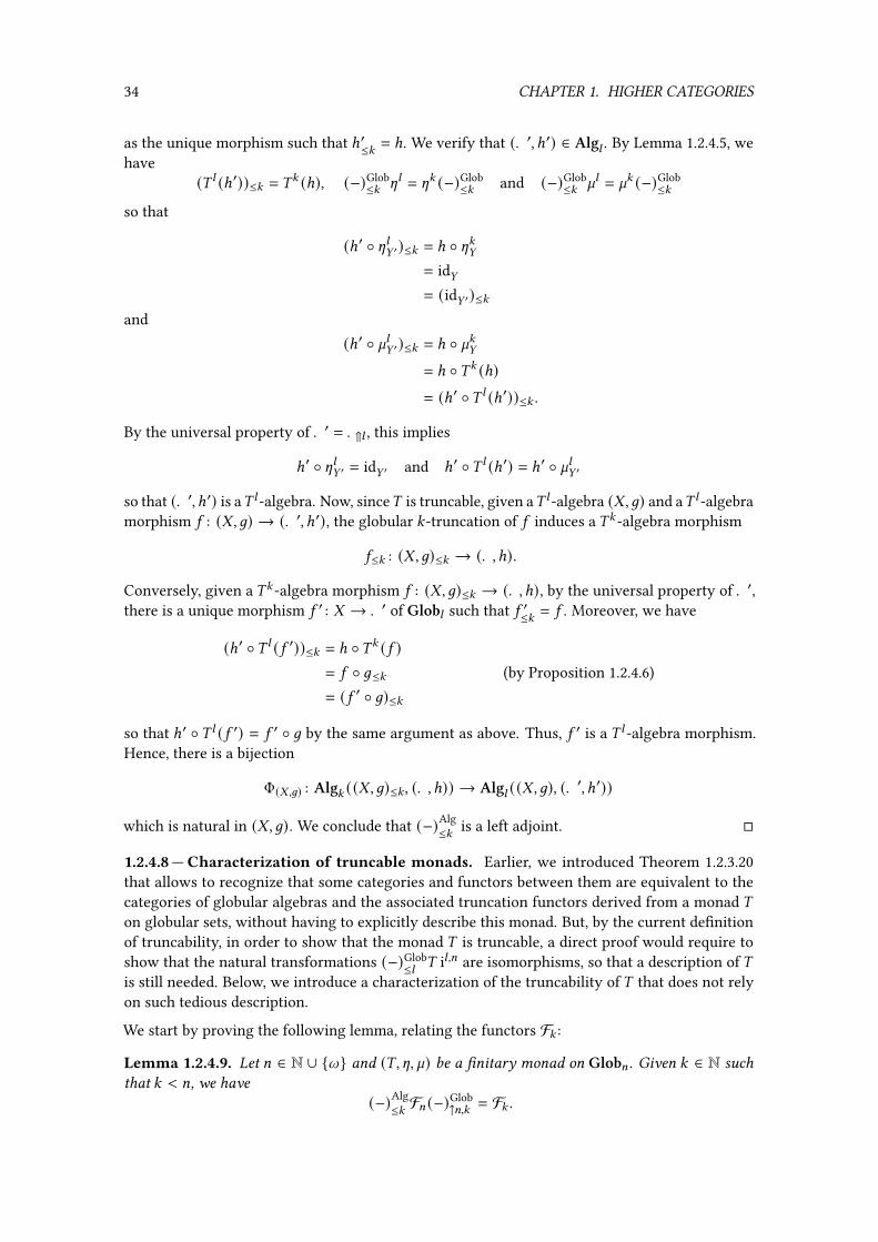
34 CHAPTER 1. HIGHER CATEGORIES

as the unique morphism such that ℎ′≤: = ℎ. We verify that (. ′, ℎ′) ∈ Alg; . By Lemma 1.2.4.5, wehave

() ; (ℎ′))≤: = ): (ℎ), (−)Glob≤: [; = [: (−)Glob

≤: and (−)Glob≤: `; = `: (−)Glob

≤:

so that

(ℎ′ ◦ [;. ′)≤: = ℎ ◦ [:.= id.= (id. ′)≤:

and(ℎ′ ◦ `;. ′)≤: = ℎ ◦ `:.

= ℎ ◦): (ℎ)= (ℎ′ ◦) ; (ℎ′))≤: .

By the universal property of . ′ = .⇑; , this implies

ℎ′ ◦ [;. ′ = id. ′ and ℎ′ ◦) ; (ℎ′) = ℎ′ ◦ `;. ′

so that (. ′, ℎ′) is a) ; -algebra. Now, since) is truncable, given a) ; -algebra (-,6) and a) ; -algebramorphism 5 : (-,6) → (. ′, ℎ′), the globular :-truncation of 5 induces a ): -algebra morphism

5≤: : (-,6)≤: → (.,ℎ).

Conversely, given a ): -algebra morphism 5 : (-,6)≤: → (.,ℎ), by the universal property of . ′,there is a unique morphism 5 ′ : - → . ′ of Glob; such that 5 ′≤: = 5 . Moreover, we have

(ℎ′ ◦) ; (5 ′))≤: = ℎ ◦): (5 )= 5 ◦ 6≤: (by Proposition 1.2.4.6)= (5 ′ ◦ 6)≤:

so that ℎ′ ◦) ; (5 ′) = 5 ′ ◦ 6 by the same argument as above. Thus, 5 ′ is a ) ; -algebra morphism.Hence, there is a bijection

Φ(-,6) : Alg: ((-,6)≤: , (.,ℎ)) → Alg; ((-,6), (. ′, ℎ′))

which is natural in (-,6). We conclude that (−)Alg≤: is a left adjoint. �

1.2.4.8 — Characterization of truncable monads. Earlier, we introduced Theorem 1.2.3.20that allows to recognize that some categories and functors between them are equivalent to thecategories of globular algebras and the associated truncation functors derived from a monad )on globular sets, without having to explicitly describe this monad. But, by the current de�nitionof truncability, in order to show that the monad ) is truncable, a direct proof would require toshow that the natural transformations (−)Glob

≤; ) i;,= are isomorphisms, so that a description of )is still needed. Below, we introduce a characterization of the truncability of ) that does not relyon such tedious description.

We start by proving the following lemma, relating the functors F: :

Lemma 1.2.4.9. Let = ∈ N ∪ {l} and (), [, `) be a �nitary monad on Glob= . Given : ∈ N suchthat : < =, we have

(−)Alg≤: F= (−)

Glob↑=,: = F: .

1.2. HIGHER CATEGORIES AS GLOBULAR ALGEBRAS 35

Proof. We �rst compute that

U: (−)Alg≤: F= (−)

Glob↑=,: = (−)Glob

≤: U=F= (−)Glob↑=,:

= (−)Glob≤: )= (−)Glob

↑=,:

= ):

= U:F: .

Moreover, writting n: and n= for the counit of the adjunctions

F: a U: and F= a U=

respectively, we have

n: (−)Alg≤: F= (−)

Glob↑=,: = (−)Glob

≤: ((U=n=) ◦ ()= i:,=U=))F= (−)Glob

↑=,: (by de�nition of (−)Alg≤:,=)

= (−)Glob≤: ((U=n

=F=) ◦ ()= i:,=)=)) (−)Glob↑=,:

= (−)Glob≤: (`

= ◦ ()= i:,= F=)) (−)Glob↑=,:

= `: (by de�nition of `: )

= n:F:

so that(−)Alg≤: F= (−)

Glob↑=,: = F:

by Theorem 1.2.1.2. �

Now, we prove that truncable monads can be characterized through the associated globularalgebras:

Proposition 1.2.4.10. Let = ∈ N ∪ {l} and (), [, `) be a �nitary monad on Glob= . Then, themonad (), [, `) is weakly truncable (resp. truncable) if and only if, for : ∈ N=−1, the naturaltransformation

(−)Alg≤: F= i:,= : F: (−)Glob

≤: ⇒ (−)Alg≤: F=

is an isomorphism (resp. an identity).

Proof. Note that the domain of (−)Alg≤: F= i:,= is the claimed one by Lemma 1.2.4.9. For : ∈ N=−1,

we have that

U: (−)Alg≤: F= i: = (−)Glob

≤: U=F= i:

= (−)Glob≤: ) i: .

The proposition follows from the fact thatU: re�ects isomorphisms (resp. identities). �

Given : ∈ N, we writej:,= : idGlob= ⇒ (−)

Glob⇑=,: (−)

Glob≤:,=

or simply j: , for the unit of the adjunction (−)Glob≤:,= a (−)

Glob⇑=,: : Glob: → Glob= . We have the

following criterion for showing the truncability of monads through their globular algebras:

Theorem 1.2.4.11. Let= ∈ N∪{l} and (), [, `) be a �nitarymonad onGlob= . The monad (), [, `)is weakly truncable if and only if, for : ∈ N=−1, the functor (−)Alg

≤:,= has a right adjoint, that wewrite (−)Alg

⇑=,: , which satis�es that j:U= (−)Alg⇑=,: is an isomorphism.

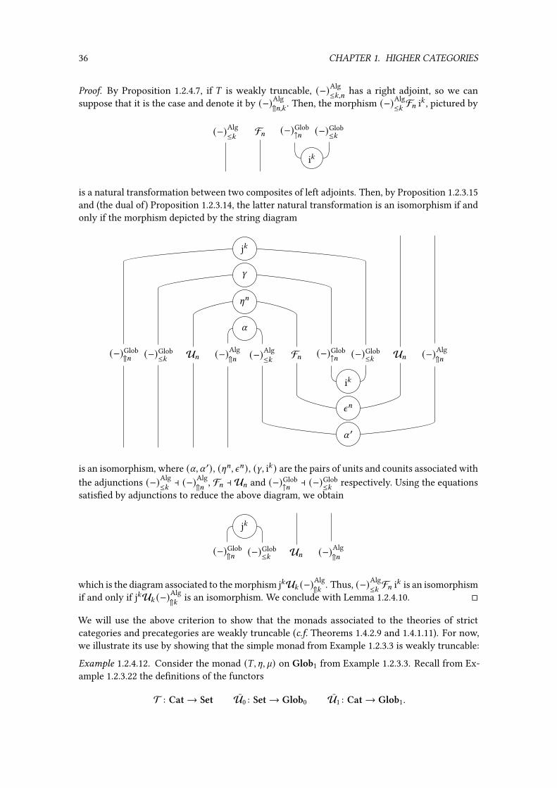
36 CHAPTER 1. HIGHER CATEGORIES

Proof. By Proposition 1.2.4.7, if ) is weakly truncable, (−)Alg≤:,= has a right adjoint, so we can

suppose that it is the case and denote it by (−)Alg⇑=,: . Then, the morphism (−)Alg

≤: F= i: , pictured by

(−)Alg≤: F= (−)Glob

↑= (−)Glob≤:

i:

is a natural transformation between two composites of left adjoints. Then, by Proposition 1.2.3.15and (the dual of) Proposition 1.2.3.14, the latter natural transformation is an isomorphism if andonly if the morphism depicted by the string diagram

(−)Glob⇑= (−)Glob

≤: U= (−)Alg⇑= (−)Alg

≤: F= (−)Glob↑= (−)Glob

≤: U= (−)Alg⇑=

U

[=

W

j:

i:

n=

U ′

is an isomorphism, where (U, U ′), ([=, n=), (W, i: ) are the pairs of units and counits associated withthe adjunctions (−)Alg

≤: a (−)Alg⇑= , F= a U= and (−)Glob

↑= a (−)Glob≤: respectively. Using the equations

satis�ed by adjunctions to reduce the above diagram, we obtain

(−)Glob⇑= (−)Glob

≤: U= (−)Alg⇑=

j:

which is the diagram associated to the morphism j:U: (−)Alg⇑: . Thus, (−)Alg

≤: F= i: is an isomorphismif and only if j:U: (−)Alg

⇑: is an isomorphism. We conclude with Lemma 1.2.4.10. �

We will use the above criterion to show that the monads associated to the theories of strictcategories and precategories are weakly truncable (c.f. Theorems 1.4.2.9 and 1.4.1.11). For now,we illustrate its use by showing that the simple monad from Example 1.2.3.3 is weakly truncable:

Example 1.2.4.12. Consider the monad (), [, `) on Glob1 from Example 1.2.3.3. Recall from Ex-ample 1.2.3.22 the de�nitions of the functors

T : Cat→ Set U0 : Set→ Glob0 U1 : Cat→ Glob1.

1.3. FREE HIGHER CATEGORIES ON GENERATORS 37

One easily veri�es that the functor T : Cat→ Set has a right adjoint G : Set→ Cat which is thecanonical functor mapping a set ( to the category whose set of 0-cells is ( and which has exactlyone 1-cell between every pair of 0-cells. For this de�nition and the one of j0, we have that j0U1Gis an isomorphism. Since, from Example 1.2.3.22, we have a commutative diagram

Cat Alg1

Set Alg0

�1

T (−)Alg≤0

�0

where �0 and �1 are equivalences of categories such that U0�0 = U0 and U1�1 = U1, thefunctor (−)Alg

≤0,1 has a right adjoint (−)Alg⇑1,0 such that j0U1(−)Alg

⇑1,0 is an isomorphism. Thus, themonad ) is truncable by Theorem 1.2.4.11.

1.3 Free higher categories on generators

Given some theory of higher categories, an important construction is the one that builds a :-cate-gory which is freely generated on a set of generators. Indeed, like for other algebraic theories,a :-category can be described by means of a presentation, i.e., by quotienting a free :-categoryby a set of relations. Such presentations are all the more interesting from a computational per-spective since they allow encoding higher categories with possibly in�nite number of cells as�nite data. For example, a formal adjunction can be described as the strict 2-category generatedby two 0-cells G and ~, two 1-cells ; : ~ → G and A : G → ~, and two 2-cells W : id~ ⇒ ; ∗0 Aand n : A ∗0 ; ⇒ idG satisfying the zigzag equations (1.3). Given a theory of higher categoriesexpressed in Batanin’s setting, i.e., as a monad (), [, `) on Glob= for some = ∈ N ∪ {l}, there areseveral free constructions that one can consider. First, the functors F: : Glob: → Alg: alreadyenable to construct the free :-category on a :-globular set. Moreover, there is a constructionwhich produces a (:+1)-category from a :-cellular extension, i.e., a pair consisting of a :-categoryand a set of (:+1)-generators. Such construction was introduced for strict categories in [Bur93].Finally, one can consider the free :-category on a :-polygraph: the latter is a system of 8-gene-rators for 8 ∈ N= which is organized inductively as cellular extensions. It di�ers from a mere:-globular set in the sense that a :-polygraph allows generators to have complex sources andtargets that are composites of other generators, whereas the sources and targets of generators or-ganized in a :-globular set can only be globes. Polygraphs were �rst introduced by Street [Str76]and Burroni [Bur93] for strict categories, and then generalized to any �nitary monad on globularsets by Batanin [Bat98a].

The aim of this section is to introduce the de�nitions of cellular extensions and polygraphstogether with the associated free constructions. Since most of the de�nitions rely on pullbacksin CAT, we �rst recall some properties of these pullbacks (Section 1.3.1). Then, we introduce cel-lular extensions together with the associated free construction for any �nitary monad on globularsets, and, in the case of a truncable monad, we show that this construction is stable, i.e., that freelyadding (:+1)-generators does not change the underlying :-category (Section 1.3.2). Finally, weintroduce polygraphs together with the associated free construction for any �nitary monad onglobular sets (Section 1.3.3). Our de�nition di�ers from the one of Batanin since ours is based oncellular extensions, whereas the one of Batanin is more direct. We moreover prove a local �nitepresentability result for the categories of polygraphs.

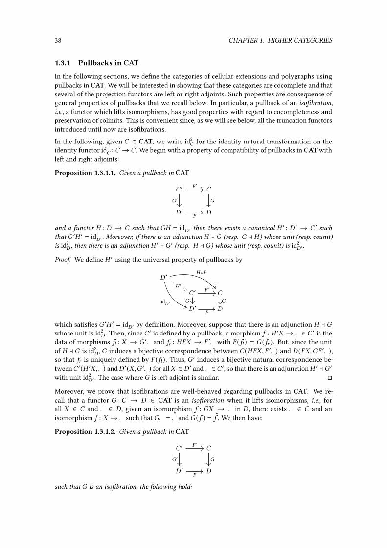
38 CHAPTER 1. HIGHER CATEGORIES

1.3.1 Pullbacks in CAT

In the following sections, we de�ne the categories of cellular extensions and polygraphs usingpullbacks in CAT. We will be interested in showing that these categories are cocomplete and thatseveral of the projection functors are left or right adjoints. Such properties are consequence ofgeneral properties of pullbacks that we recall below. In particular, a pullback of an iso�bration,i.e., a functor which lifts isomorphisms, has good properties with regard to cocompleteness andpreservation of colimits. This is convenient since, as we will see below, all the truncation functorsintroduced until now are iso�brations.

In the following, given � ∈ CAT, we write id2� for the identity natural transformation on the

identity functor id� : � → � . We begin with a property of compatibility of pullbacks in CAT withleft and right adjoints:

Proposition 1.3.1.1. Given a pullback in CAT

� ′ �

� ′ �

� ′

�′ �

�

and a functor � : � → � such that �� = id� , then there exists a canonical � ′ : � ′ → � ′ suchthat � ′� ′ = id�′ . Moreover, if there is an adjunction � a � (resp. � a � ) whose unit (resp. counit)is id2

� , then there is an adjunction � ′ a � ′ (resp. � a �) whose unit (resp. counit) is id2�′ .

Proof. We de�ne � ′ using the universal property of pullbacks by

� ′

� ′ �

� ′ �

�◦�

� ′

id�′

� ′

�′ �

�

which satis�es � ′� ′ = id�′ by de�nition. Moreover, suppose that there is an adjunction � a �whose unit is id2

� . Then, since � ′ is de�ned by a pullback, a morphism 5 : � ′- → . ∈ � ′ is thedata of morphisms 5; : - → � ′. and 5A : ��- → � ′. with � (5; ) = � (5A ). But, since the unitof � a � is id2

� , � induces a bijective correspondence between � (��-, � ′. ) and � (�-,�� ′. ),so that 5A is uniquely de�ned by � (5; ). Thus, � ′ induces a bijective natural correspondence be-tween� ′(� ′-,. ) and� ′(-,� ′. ) for all- ∈ � ′ and. ∈ � ′, so that there is an adjunction� ′ a � ′with unit id2

�′ . The case where � is left adjoint is similar. �

Moreover, we prove that iso�brations are well-behaved regarding pullbacks in CAT. We re-call that a functor � : � → � ∈ CAT is an iso�bration when it lifts isomorphisms, i.e., forall - ∈ � and . ∈ � , given an isomorphism 5 : �- → . in � , there exists . ∈ � and anisomorphism 5 : - → . such that �. = . and � (5 ) = 5 . We then have:

Proposition 1.3.1.2. Given a pullback in CAT

� ′ �

� ′ �

� ′

�′ �

�

such that � is an iso�bration, the following hold:

1.3. FREE HIGHER CATEGORIES ON GENERATORS 39

(i) � ′ is an iso�bration,

(ii) given a small category � , if � and � ′ have all � -colimits and � and � preserve them, then � ′

has all � -colimits and � ′ and � ′ preserve them.

Proof. Proof of (i): Let - ∈ � ′, .! ∈ � ′ and \! : � ′- → .! be an isomorphism. Then, since �is an iso�bration, there is .' ∈ � and an isomorphism \' : � ′- → .' such that � (\!) = � (\').Moreover, � (\−1

!) = � (\−1

') so that (\!, \') : - → (.!, .') is an isomorphism of � ′.

Proof of (ii): Let 3 : � → � ′ be a functor, which is the data of 3! : � → � ′ and 3' : � → � . Then,there are colimit cocones (?!,8 : 3! (8) → -!)8∈� and (?',8 : 3' (8) → -')8∈� . Since both � and �preserve colimits, both

(� (?!,8) : � (3! (8)) → � (-!))8∈� and (� (?',8) : � (3! (8)) → � (-'))8∈�

are colimit cocones for � ◦ 3! . So there exists an isomorphism \ : � (-!) → � (-') between thetwo cocones. Since � is an iso�bration, we can suppose that � (-!) = � (-') and \ = id

� (-!) .Thus, we have a cocone ((?!,8 , ?',8) : 3 (8) → (-!, -'))8 on 3 , and we easily verify that it is acolimit cocone. �

Remark 1.3.1.3. Pullbacks in CAT should normally raise suspicion since strict limits are not well-behaved in CAT in general. Indeed, a limit cone in CAT on a diagram is not stable when replacingsome functors of the diagram by isomorphic functors. Moreover, the limit cone is de�ned up toisomorphism, and not up to equivalence of categories. To solve this problem, one usually considersa weaker notion of limits, where the triangles of cones commute only up to isomorphisms, aswith weighted bilimits [MP89]. But the strict limit on a diagram is generally not equivalentto the associated weighted bilimit. However, introducing weighted bilimits here would be anunnecessary pain for what we want to do, since the pullbacks along iso�brations are equivalentto the weighted bipullbacks (see [MP89, Proposition 5.1.1]).

We now verify that several functors of interest to us are iso�brations:

Proposition 1.3.1.4. Given : ∈ N, the functor (−)Glob≤:,:+1 is an iso�bration.

Proof. Given - ∈ Glob:+1 and an isomorphism � : -≤: → . in Glob: , we de�ne . ∈ Glob:+1by .≤: = . and .:+1 = -:+1 and such that the :-source and :-target operations of . are de�nedas � ◦ m−

:and � ◦ m+

:respectively. Then, � is lifted by the isomorphism � : - → . of Glob:+1

de�ned by �≤: = � and �:+1 = 1-:+1 . �

Proposition 1.3.1.5. Let = ∈ N∪ {l} and (), [, `) be a �nitary monad on Glob= . Given : ∈ N=−1,the functor (−)Alg

≤:,:+1 is an iso�bration.

Proof. Given an object (-,6 : ):+1- → - ) of Alg:+1 and an isomorphism � : (-,6)≤: → (. , ℎ)of Alg: , by Proposition 1.3.1.4, there is . ∈ Glob:+1 and an isomorphism � : - → . in Glob:+1such that �≤: = � . We can equip . with a structure of):+1-algebra by de�ning ℎ : ):+1. → . as

ℎ = � ◦ 6 ◦ ():+1(� ))−1

40 CHAPTER 1. HIGHER CATEGORIES

so that � : (-,6) → (.,ℎ) is a morphism of Alg:+1. It remains to show that (.,ℎ)≤: = (. , ℎ). Byde�nition of . , we have .≤: = . . Moreover, we compute that

ℎ≤: ◦ ((−)Glob≤: ):+1 i: ). ◦): (� )

= ℎ≤: ◦ ():+1(� ))≤: ◦ ((−)Glob≤: ):+1 i: )- (by naturality of i: )

= � ◦ 6≤: ◦ ((−)Glob≤: ):+1 i: )- (since � is a morphism of Alg:+1)

= ℎ ◦): (� ) (since � is a morphism of Alg: )

so that ℎ≤: ◦ ((−)Glob≤: ):+1 i: ). = ℎ, i.e., (.,ℎ)≤: = (. , ℎ). Thus, � , as a morphism of Alg: , is lifted

by � . Hence, (−)Alg≤:,:+1 is an iso�bration. �

1.3.2 Cellular extensions

In this section, we introduce the notion of :-cellular extension, which describes a :-category (forsome theory of higher categories) equipped with a set of (:+1)-generators. We moreover givethe construction of the free (:+1)-category on a :-cellular extension together with more speci�cresults when the theory we are considering is associated with a truncable monad.

1.3.2.1 — De�nition. Let= ∈ N∪{l} and (), [, `) be a �nitary monad onGlob= . Given: ∈ N=−1,we de�ne the category Alg+

:of :-cellular extensions as the pullback

Alg+:

Glob:+1

Alg: Glob:

G:+1

A: (−)Glob≤:

U:

We verify that:

Proposition 1.3.2.2. The functor A: is an iso�bration and has both left and right adjoints.

Proof. This is a consequence of Proposition 1.3.1.4 and Proposition 1.3.1.2. �

There is a functorV: : Alg:+1 → Alg+:

de�ned as the factorization arrow

Alg:+1

Alg+:

Glob:+1

Alg: Glob:

U:+1

(−)Alg≤:

V:

A:

G:+1

(−)Glob≤:

U:

.

There is an operation which produces a (:+1)-category from a :-cellular extension. It is the leftadjoint toV: , that exists by the following property:

Theorem 1.3.2.3. V: has a left adjoint.

1.3. FREE HIGHER CATEGORIES ON GENERATORS 41

Proof. Let U: be the unit of the adjunction (−)Alg↑:+1,: a (−)

Alg≤:,:+1, and n; be the counit of the ad-

junction F; a U; for ; ∈ {:, : + 1}. Let

ΦL : Alg:+1((−)Alg↑:+1,−) ⇒ Alg: (−, (−)

Alg≤: )

ΨL : Alg: ((−)Alg↑:+1F: (−),−) ⇒ Glob: (−,U: (−)Alg

≤:,:+1)

ΦR : Alg:+1(F:+1(−),−) ⇒ Glob:+1(−,U:+1(−))

ΨR : Glob:+1(F:+1(−)Glob↑:+1,: ,−) ⇒ Glob: (−, (−)Glob

≤: U:+1(−))

be the natural bijections derived from the associated adjunctions de�ned in Paragraphs 1.2.2.3,1.2.3.1 and 1.2.3.6. Note that these bijections can be de�ned using the units of the adjunctions.For example, given � ∈ Alg: and � ∈ Alg:+1, ΦL maps a morphism 5 : �↑:+1 → � ∈ Alg:+1 tothe morphism 5≤: ◦ U:� : � → �≤: ∈ Alg: . Since

F:+1(−)Glob↑:+1 and (−)Alg

↑:+1F:

are both left adjoint toU: (−)Alg≤:,:+1 = (−)

Glob≤: U:+1, the natural morphism

\ : F:+1(−)Glob↑:+1,: ⇒ (−)

Alg↑:+1F:

de�ned as the composite

\ = (n:+1(−)Alg↑:+1,:F: ) ◦ (F:+1 i: U:+1(−)Alg

↑:+1,:F: ) ◦ (F:+1(−)Glob↑:+1,:U:U

:F: ) ◦ (F:+1(−)Glob↑:+1,:[

: )

which can be represented by

F:+1 (−)Glob↑:+1,:

(−)Alg↑:+1,:

F:

\ =

F:+1 (−)Glob↑:+1,:

(−)Alg↑:+1,:

F:

[:

U:

i:

n:+1

=

is an isomorphism as a consequence of Propositions 1.2.3.14 and 1.2.3.15. In the following, given amorphism 5 : - → . of a category C, we write 5 ∗ : C(., / ) → C(-,/ ) for the function 6 ↦→ 6◦ 5for all / ∈ C. One can verify using the zigzag equations that the natural transformation \ makesthe diagram

Alg:+1((F:/ )↑:+1, �) Glob: (/,U: (�≤: ))

Alg:+1(F:+1(/↑:+1), �) Glob: (/, (U:+1�)≤: )(\/ )∗

ΨL/,�

ΨR/,�

(1.6)

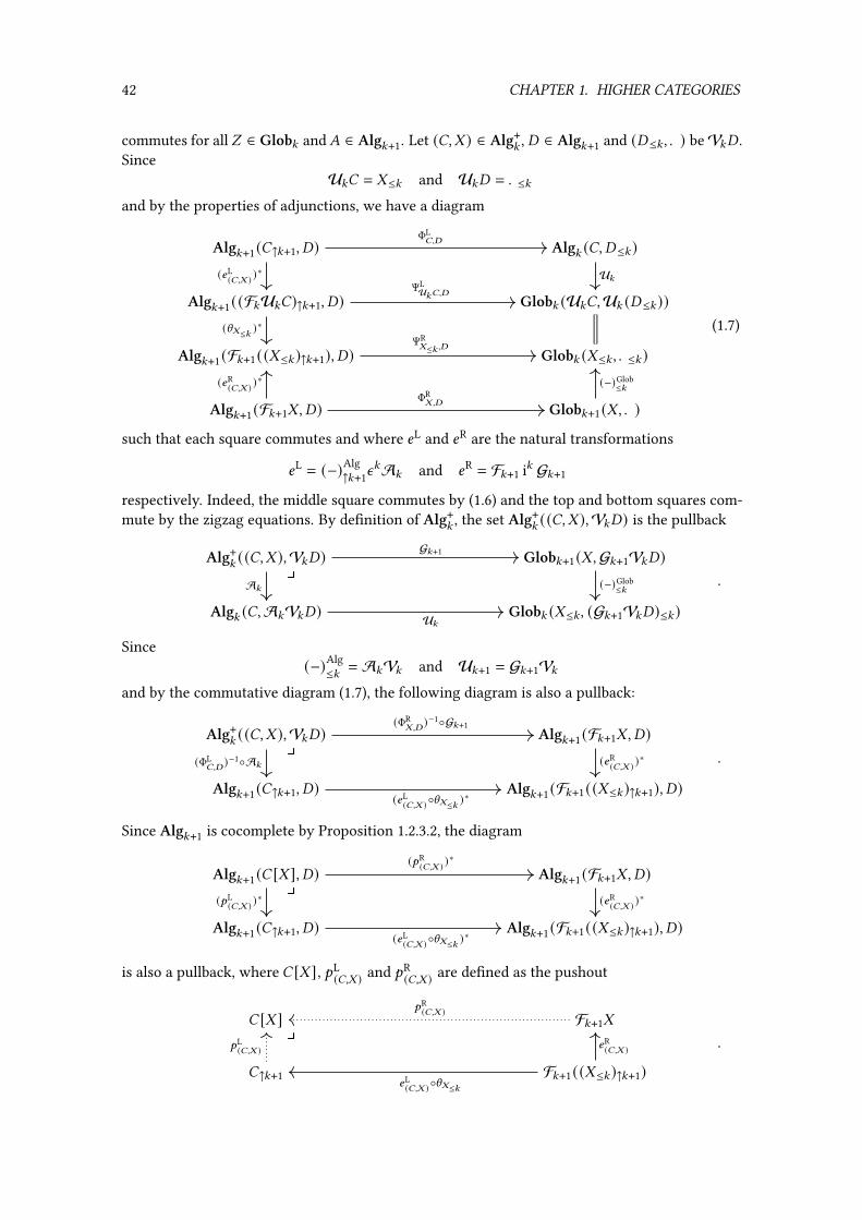
42 CHAPTER 1. HIGHER CATEGORIES

commutes for all / ∈ Glob: and� ∈ Alg:+1. Let (�,- ) ∈ Alg+:, � ∈ Alg:+1 and (�≤: , . ) beV:� .

SinceU:� = -≤: and U:� = .≤:

and by the properties of adjunctions, we have a diagram

Alg:+1(�↑:+1, �) Alg: (�, �≤: )

Alg:+1((F:U:�)↑:+1, �) Glob: (U:�,U: (�≤: ))

Alg:+1(F:+1((-≤: )↑:+1), �) Glob: (-≤: , .≤: )

Alg:+1(F:+1-, �) Glob:+1(-,. )

(4L(�,- ) )

∗ U:

(\-≤: )∗

(4R(�,- ) )

∗ (−)Glob≤:

ΦL�,�

ΨLU:�,�

ΨR-≤: ,�

ΦR-,�

(1.7)

such that each square commutes and where 4L and 4R are the natural transformations

4L = (−)Alg↑:+1n

:A: and 4R = F:+1 i: G:+1respectively. Indeed, the middle square commutes by (1.6) and the top and bottom squares com-mute by the zigzag equations. By de�nition of Alg+

:, the set Alg+

:((�,- ),V:�) is the pullback

Alg+:((�,- ),V:�) Glob:+1(-,G:+1V:�)

Alg: (�,A:V:�) Glob: (-≤: , (G:+1V:�)≤: )

G:+1

A: (−)Glob≤:

U:

.

Since(−)Alg≤: = A:V: and U:+1 = G:+1V:

and by the commutative diagram (1.7), the following diagram is also a pullback:

Alg+:((�,- ),V:�) Alg:+1(F:+1-, �)

Alg:+1(�↑:+1, �) Alg:+1(F:+1((-≤: )↑:+1), �)

(ΦR-,�)−1◦G:+1

(ΦL�,�)−1◦A: (4R

(�,- ) )∗

(4L(�,- )◦\-≤: )

∗

.

Since Alg:+1 is cocomplete by Proposition 1.2.3.2, the diagram

Alg:+1(� [- ], �) Alg:+1(F:+1-, �)

Alg:+1(�↑:+1, �) Alg:+1(F:+1((-≤: )↑:+1), �)

(?R(�,- ) )

∗

(?L(�,- ) )

∗ (4R(�,- ) )

∗

(4L(�,- )◦\-≤: )

∗

is also a pullback, where � [- ], ?L(�,- ) and ?R

(�,- ) are de�ned as the pushout

� [- ] F:+1-

�↑:+1 F:+1((-≤: )↑:+1)

?R(�,- )

?L(�,- ) 4R

(�,- )

4L(�,- )◦\-≤:

.

1.3. FREE HIGHER CATEGORIES ON GENERATORS 43

Thus, there is an isomorphism

Alg:+1(� [- ], �) ' Alg+:((�,- ),V:�)

which is natural in � . Hence,V: admits a left adjoint. �

The operation (�,- ) ↦→ � [- ] de�ned in the proof of Theorem 1.3.2.3 extends to a functor

−[−]: : Alg+:→ Alg:+1

that we often write −[−] when there is no ambiguity on : , and which is left adjoint toV: . Theimage � [- ] of some (�,- ) ∈ Alg+: is called the free extension on (�,- ).Example 1.3.2.4. Consider the monad (), [, `) on Glob1 de�ned in Example 1.2.3.3. A 0-cellularextension (�,- ) is then essentially the data of a set �0 of 0-cells, a set -1 of 1-generators, andfunctions d−0 , d

+0 : -1 → �0, i.e., a graph. Moreover, the 1-category � [- ] is the image of (�,- )

seen as a graph by the left adjoint to the functor Cat→ Gph de�ned in Example 1.1.2.10.

Remark 1.3.2.5. Theorem 1.3.2.3 is a particular case of the fact that the category of locally pre-sentable categories and right adjoints are closed under weak limits (see [Bir84] and the endof [MP89, §5.1]). Since we did not introduce those limits, we explicitly described the constructionof the left adjoint ofV: in the case of a strict pullback.

1.3.2.6 — The truncable case. Let = ∈ N ∪ {l} and (), [, `) be a �nitary monad on Glob= . Inthis paragraph, we consider the case where) is a truncable monad, and show that the underlying:-category of a :-cellular extension is preserved by −[−]: . For this purpose, we �rst prove thatthe functor (−)Alg

↑:+1,: preserves the underlying :-category. A direct proof method for this would

be to explicitly describe the functor (−)Alg↑:+1,: , but that would be tedious and tiresome. We prefer

an indirect method based on a monadicity argument. We start by giving another description ofthe images of free :-categories by (−)Alg

↑:+1:

Proposition 1.3.2.7. If ) is truncable, then, given : ∈ N=−1 and - ∈ Glob: , (−)Alg≤:,:+1 induces a

natural isomorphism

Alg:+1(F:+1(-↑:+1),−) → Alg: (F: (- ), (−)Alg≤: ).

Proof. Given (.,ℎ : ):+1. → . ) ∈ Alg:+1, consider the function

Θ(.,ℎ) : Alg:+1(F:+1(-↑:+1), (.,ℎ)) → Alg: (F: (- ), (.,ℎ)≤: )

induced by (−)Alg≤: . This function is well-de�ned, since, by the de�nitions of F: and F:+1, and by

the fact that ) is truncable, we have (−)Alg≤: F:+1 = F: (−)

Glob≤: , so that (−)Alg

≤: F:+1(−)Glob↑:+1 = F: . We

�rst show that Θ(.,ℎ) is a monomorphism. Let 5 : F:+1(-↑:+1) → (.,ℎ) be a morphism of Alg:+1.We compute that

():+1 i: ):+1(−)Glob↑:+1)- ◦ ()

:+1(−)Glob↑:+1[

: )-= ():+1 i: ):+1(−)Glob

↑:+1)- ◦ ():+1(−)Glob

↑:+1(−)Glob≤: [:+1(−)Glob

↑:+1)- (by de�nition of [: )

= ():+1[:+1(−)Glob↑:+1)- ◦ ()

:+1 i: (−)Glob↑:+1)- (by naturality)

= ():+1[:+1(−)Glob↑:+1)- (since i: (−)Glob

↑:+1 = id(−)Glob↑:+1

)

44 CHAPTER 1. HIGHER CATEGORIES

and

ℎ ◦):+1(5 ) ◦ ():+1[:+1(−)Glob↑:+1)- = 5 ◦ `:+1-↑:+1

◦ ():+1[:+1)-↑:+1 = 5 .

Thus, there is a diagram

):+1(-↑:+1) ):+1(():- )↑:+1) ):+1(.≤: )↑:+1

):+1(-↑:+1) ):+1):+1(-↑:+1) ):+1. .

():+1 (−)Glob↑:+1[

: )- ):+1 ( (5≤: )↑:+1)

():+1 i: ):+1 (−)Glob↑:+1)- ():+1 i: ).

():+1[:+1 (−)Glob↑:+1)- ):+1 (5 ) ℎ

where the �rst square commutes by the �rst calculation, the second square commutes by naturalityand the bottom row is equal to 5 by the second computation. Thus, 5 can be recovered from 5≤: ,which proves that Θ(.,ℎ) is injective.

We now show that Θ(.,ℎ) is surjective. Let 5 : ():-, `- ) → (.,ℎ)≤: be a morphism in Alg: .We de�ne a morphism 5 ′ : ):+1(-↑:+1) → . of Glob:+1 as the composite

):+1(-↑:+1) ):+1(():- )↑:+1) ):+1((.≤: )↑:+1) ):+1. .

():+1 (−)Glob↑:+1[

: )- ):+1 (5↑:+1) ():+1 i: ). ℎ.

We compute that

ℎ ◦):+1(5 ′) = ℎ ◦):+1(ℎ) ◦):+1):+1(i:. ◦5↑:+1 ◦ ([:- )↑:+1)

= ℎ ◦ `:+1. ◦):+1):+1(i:. ◦5↑:+1 ◦ ([:- )↑:+1) (since ℎ ∈ Alg:+1)

= ℎ ◦):+1(i:. ◦5↑:+1 ◦ ([:- )↑:+1) ◦ `

:+1-↑:+1

(by naturality of `:+1)

= 5 ′ ◦ `:+1-↑:+1

so 5 ′ induces a morphism in Alg:+1. Moreover, we have

5 ′≤: = ℎ≤: ◦ ():+1(i:. ))≤: ◦): (5 ) ◦ ():[: )-

= ℎ≤: ◦): ((i:. )≤: ) ◦): (5 ) ◦ ():[: )- (since ) is truncable)

= ℎ≤: ◦): (5 ) ◦ ():[: )- (since (−)Glob≤: i: = id(−)Glob

≤:)

= 5 ◦ `:- ◦ ():[: )- (by Proposition 1.2.4.6)

= 5

so that 5 ′≤: = 5 , which proves that Θ(.,ℎ) is surjective. Finally, it is clear from the de�nitionof Θ(.,ℎ) that it is natural in . , which concludes the proof. �

Given : ∈ N=−1, let [A,: be the natural transformation

[A,: : idAlg: ⇒ (−)Alg≤: (−)

Alg↑:+1

often simply denoted [A, which is the unit of the adjunction (−)Alg↑:+1 a (−)

Alg≤: . We are going to

show that [A is an isomorphism when ) is truncable. First, Proposition 1.3.2.7 implies that therestriction of [A to free :-algebras is an isomorphism:

Proposition 1.3.2.8. If ) is truncable, then, given : ∈ N= , [AF: is a natural isomorphism.

1.3. FREE HIGHER CATEGORIES ON GENERATORS 45

Proof. Given - ∈ Glob: , we prove that ([AF: )- is an isomorphism. By adjunction properties,the functor

Alg: (F:-, (−)Alg≤: ) : Alg:+1 → Set

is representable by the pair ((F:- )↑:+1, ([AF: )- ), and, by Proposition 1.3.2.7, it is also repre-sentable by the pair (F:+1(-↑:+1), idF:- ). The sequence of bijections

Alg:+1((F:- )↑:+1, (F:- )↑:+1) ' Alg: (F:-, ((F:- )↑:+1)≤: ) ' Alg:+1(F:+1(-↑:+1), (F:- )↑:+1)

sends id(F:- )↑:+1 to a morphism q : F:+1(-↑:+1) → (F:- )↑:+1, and one can verify that the latteris an isomorphism by constructing its inverse in a dual manner. Moreover, by representabilityand naturality, we have ([AF: )- = q≤: ◦ idF:- = q≤: , so that ([AF: )- is an isomorphism. �

Since Alg: is the category of algebras of (): , [: , `: ), every object of Alg: can be expressed as aquotient of free :-algebras, so that the isomorphism of Proposition 1.3.2.8 extends to Alg: as awhole:

Proposition 1.3.2.9. If ) is truncable, then [A is an isomorphism.

Proof. Given � ∈ Alg: , we prove that [A�

is an isomorphism. Let n: be the counit of the ad-junction F: a U: (concretely, n:(-,ℎ) = ℎ for (-,ℎ) ∈ Alg: ). By the naturality of [A, we have adiagram

F:U:F:U:� F:U:� �

((F:U:F:U:�)↑:+1)≤: ((F:U:�)↑:+1)≤: (�↑:+1)≤:

(F:U:n: )�

(n: F:U: )�

([AF:U: F:U: )�

n:�

([AF:U: )� [A�

( (−)Alg≤: (−)

Alg↑:+1F:U:n

: )�

( (−)Alg≤: (−)

Alg↑:+1n

: F:U: )�

( (−)Alg≤: (−)

Alg↑:+1n

: )�

where the two squares on the left corresponding to F:U:n: and n:F:U: respectively, and thesquare on the right commute. Since the functor U: is monadic by de�nition, the top row is acoequalizer (see [Bor94b, Lemma 4.3.3] for example). Moreover, since both (−)Alg

≤: and (−)Alg↑:

preserves colimits (both are left adjoints by Propositions 1.2.3.7 and 1.2.4.7), the bottom row is acoequalizer too. By Proposition 1.3.2.8, the two vertical arrows on the left are isomorphisms, sothat [A

�is an isomorphism. �

We can conclude a conservation result for the underlying:-category of (:+1)-categories producedby −[−]: :

Proposition 1.3.2.10. If ) is truncable, then, given : ∈ N= and (�,- ) ∈ Alg+: , there is an isomor-phism � ' � [- ]≤: which is natural in (�,- ).

Proof. Recall that � [- ] was de�ned in the proof of Theorem 1.3.2.3 as the pushout

� [- ] F:+1-

�↑:+1 F:+1((-≤: )↑:+1)

?R(�,- )

?L(�,- ) 4R

(�,- )

4L(�,- )◦\-≤:

.

46 CHAPTER 1. HIGHER CATEGORIES

By Proposition 1.2.4.7, the following diagram is also a pushout

� [- ]≤: (F:+1- )≤:

(�↑:+1)≤: (F:+1((-≤: )↑:+1))≤:

(?R(�,- ) )≤:

(?L(�,- ) )≤: (4R

(�,- ) )≤:

(4L(�,- )◦\-≤: )≤:

.

Since ) is truncable, we have (−)Alg≤: F:+1 = F: (−)

Glob≤: . Thus,

(4R)≤: = (−)Alg≤: F:+1 i: G:+1

= F: (−)Glob≤: i: G:+1

= idF: (−)Glob≤: G:+1

(since (i: )≤: = idGlob: )

so that (4R(�,- ) )≤: = idF: (-≤: ) . Hence, (?L

(�,- ) )≤: is an isomorphism, since the pushout of anisomorphism is an isomorphism. By Proposition 1.3.2.9, we conclude that the composite

� (�↑:+1)≤: � [- ]≤:[A�

(?L(�,- ) )≤:

is an isomorphism. �

Remark 1.3.2.11. If ) is truncable, given : ∈ N= , by Proposition 1.3.1.5, we can suppose that wechose −[−]: so that the isomorphism of Proposition 1.3.2.10 is the identity. When such a choiceis made, we have � [- ]≤: = � for all :-cellular extension (�,- ).

1.3.3 Polygraphs

In this section we recall the de�nition and several properties of polygraphs, that were �rst intro-duced by Street [Str76] for strict 2-categories (under the name computads), and then rediscoveredand extended by Burroni [Bur93] to strict:-categories, and �nally generalized by Batanin [Bat98a]to all algebraic globular higher categories. Polygraphs are structures that are inductively cellularextensions, and which allow to specify a system of generators for :-categories whose sourcesand targets are composites of other generators. They will play an important role in the followingchapters.

1.3.3.1 — Another de�nition of cellular extensions. Let= ∈ N∪{l} and (), [, `) be a �nitarymonad on Glob= . Before de�ning polygraphs, we �rst provide an alternative de�nition of Alg:which is simpler than the one based on pullbacks given in Paragraph 1.3.2.1.

Proposition 1.3.3.2. Given : ∈ N=−1, the category Alg+:is isomorphic to the category

– whose objects are the pairs (�, () where � ∈ Alg: and ( is a set, equipped with two functions

d−:, d+:

: ( → �:

such that mn:−1 ◦ d−

:= mn

:−1 ◦ d+:for n ∈ {−, +},

– and whose morphisms between two such pairs (�, () and (� ′, ( ′) are the pairs (�, 5 ) where

� : � → � ′ ∈ Alg: and 5 : ( → ( ′ ∈ Set

and such that dn:◦5 = �: ◦ dn

:for n ∈ {−, +}.

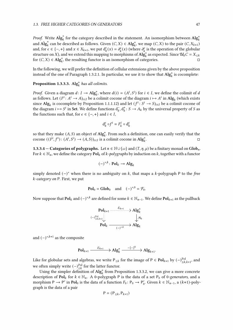
1.3. FREE HIGHER CATEGORIES ON GENERATORS 47

Proof. Write Alg+: for the category described in the statement. An isomorphism between Alg+:

and Alg+: can be described as follows. Given (�,- ) ∈ Alg+:, we map (�,- ) to the pair (�,-:+1)

and, for n ∈ {−, +} and G ∈ -:+1, we put dn:(G) = mn

:(G) (where mn

:is the operation of the globular

structure on- ), and we extend this mapping to morphisms of Alg+:

as expected. SinceU:� = -≤:for (�,- ) ∈ Alg+

:, the resulting functor is an isomorphism of categories. �

In the following, we will prefer the de�nition of cellular extensions given by the above propositioninstead of the one of Paragraph 1.3.2.1. In particular, we use it to show that Alg+

:is cocomplete:

Proposition 1.3.3.3. Alg+:has all colimits.

Proof. Given a diagram 3 : � → Alg+:, where 3 (8) = (�8 , (8) for 8 ∈ � , we de�ne the colimit of 3

as follows. Let (� 8 : �8 → �)8∈� be a colimit cocone of the diagram 8 ↦→ �8 in Alg: (which existssince Alg: is cocomplete by Proposition 1.1.1.12) and let (5 8 : (8 → ()8∈� be a colimit cocone ofthe diagram 8 ↦→ (8 in Set. We de�ne functions d−

:, d+:

: ( → �: by the universal property of ( asthe functions such that, for n ∈ {−, +} and 8 ∈ � ,

dn:◦5 8 = � 8

:◦ dn

:

so that they make (�, () an object of Alg+:. From such a de�nition, one can easily verify that the

cocone ((� 8 , 5 8) : (�8 , (8) → (�, ())8∈� is a colimit cocone in Alg+:. �

1.3.3.4 — Categories of polygraphs. Let= ∈ N∪{l} and (), [, `) be a �nitary monad on Glob= .For : ∈ N= , we de�ne the category Pol: of :-polygraphs by induction on : , together with a functor

(−)∗,: : Pol: → Alg:

simply denoted (−)∗ when there is no ambiguity on : , that maps a :-polygraph P to the free:-category on P. First, we put

Pol0 = Glob0 and (−)∗,0 = F0.

Now suppose that Pol: and (−)∗,: are de�ned for some : ∈ N=−1. We de�ne Pol:+1 as the pullback

Pol:+1 Alg+:

Pol: Alg:

(−)Pol≤:,:+1

E:+1

A:

(−)∗,:

and (−)∗,:+1 as the composite

Pol:+1 Alg+:

Alg:+1E:+1 −[−]: .

Like for globular sets and algebras, we write P≤: for the image of P ∈ Pol:+1 by (−)Pol≤:,:+1, and

we often simply write (−)Pol≤: for the latter functor.

Using the simpler de�nition of Alg+:

from Proposition 1.3.3.2, we can give a more concretedescription of Pol: for : ∈ N= . A 0-polygraph P is the data of a set P0 of 0-generators, and amorphism P → P′ in Pol0 is the data of a function �0 : P0 → P′0. Given : ∈ N=−1, a (:+1)-poly-graph is the data of a pair

P = (P≤: , P:+1)

48 CHAPTER 1. HIGHER CATEGORIES

where P≤: is a :-polygraph and P:+1 is a set of (:+1)-generators, together with functions

d−:, d+:

: P:+1 → ((P≤: )∗):

such thatmn:−1 ◦ d−

:= mn

:−1 ◦ d+:

for n ∈ {−, +}, where m−:−1, m

+:−1 : ((P≤: )∗): → ((P≤: )∗):−1 are the source and target operations

of the :-category (P≤: )∗. Moreover, a morphism P→ P′ in Pol:+1 is the data of a pair (�≤: , �=+1)where �≤: : P≤: → P′≤: is a morphism of Pol: and �=+1 : P=+1 → P′=+1 is a function such that

dn:◦�=+1 = (�≤: )∗ ◦ dn

:

for n ∈ {−, +}, i.e., a (:+1)-generator 6 is mapped by �=+1 to a generator 6′ whose :-source and:-target are exactly the images of the :-source and :-target of 6 by (�≤: )∗.Remark 1.3.3.5. Note that the diagram

Pol:+1 Glob:+1

Pol: Glob:

G:+1E:+1

(−)Pol≤: (−)Glob

≤:

U: (−)∗,:

(1.8)

is a pullback, since Alg+:

is de�ned as a pullback and the concatenation of two pullbacks is still apullback.In order to better handle side conditions, we use the convention that

Alg+−1 = Glob0, E0 = idGlob0, and −[−]0 = F0

so that (−)∗,0 = −[−]0 ◦ E0. We then have:

Proposition 1.3.3.6. For : ∈ N= , the following hold:

(i) Pol: is cocomplete,

(ii) the functors (−)∗,: and E: preserve colimits,

(iii) when : > 0, the functor (−)Pol≤:−1,: lifts isomorphisms and has both a left and a right adjoint.

Proof. We show this property by induction on : . The category Pol0 = Glob0 is certainly cocom-plete and, since F0 is a left adjoint, the functor (−)∗,0 = F0 preserves colimits and so does thefunctor E0 = idGlob0

. So suppose that : > 0. By induction hypothesis and Proposition 1.3.3.3,both Pol:−1 and Alg+

:are cocomplete. Moreover, by Proposition 1.3.2.2, the functor A:−1 pre-

serves colimits, lifts isomorphisms and has both a left and a right adjoint. So, by Proposition 1.3.1.2,we deduce that Pol: is cocomplete, the functor E: preserves colimits, and the functor (−)Pol

≤:−1,:lift isomorphisms and has both a left and a right adjoint. Finally, since −[−]:−1 is a left adjoint,the functor (−)∗,:+1 = (−)∗ ◦ E: preserves colimits. �

Given 8, : ∈ N such that 8 ≤ : < = + 1, we write

(−):8 : Pol: → Set

or simply (−)8 when there is no ambiguity on : , for the functor which maps a :-polygraph P toits set of 8-generators P8 . We can re�ne Proposition 1.3.3.6(i) and say that colimits are computeddimensionwise:

1.3. FREE HIGHER CATEGORIES ON GENERATORS 49

Proposition 1.3.3.7. Given 8, : ∈ N= such that 8 ≤ : , the functor (−):8 preserves colimits.

Proof. We show this property by induction on : − 8 . When : = 8 , we have that (−):8 = � ◦ E:where � is the functor

� : Alg+:→ Set

which maps (�,- ) ∈ Alg+:

to the set of (:+1)-generators - . By Proposition 1.3.3.6 and the proofof Proposition 1.3.3.3, both E: and � preserve colimits, so that (−):8 preserves colimits. Otherwise,if : > 8 , then note that (−):8 = (−):−1

8 ◦ (−)Pol≤:−1 where, by Proposition 1.3.3.6 and induction

hypothesis, both (−)Pol≤:−1 and (−):−1

8 preserve colimits, so that (−):8 preserves colimits, whichconcludes the induction. �

In the case where ) is truncable, given :, ; ∈ N with : < ; , the underlying :-category of the free;-category on an ;-polygraph is only determined by the underlying :-polygraph, as stated by thefollowing proposition:

Proposition 1.3.3.8. If ) is truncable, then, given : ∈ N such that : < = and a (:+1)-polygraph,there exists an isomorphism (P∗)≤: ' (P≤: )∗.

Proof. By de�nition of (−)∗,: , we have

P∗ = (P≤: )∗ [P:+1]

so that the wanted isomorphism comes from Proposition 1.3.2.10. �

Remark 1.3.3.9. When ) is truncable, under the assumption of Remark 1.3.2.11, the isomorphismgiven by Proposition 1.3.3.8 is the identity. This enables to simplify some notations: given:, ; ∈ N=with : ≤ ; and an ;-polygraph P, we write directly P∗≤: for both (P∗)≤: and (P≤: )∗, and P∗

:for

both (P∗): and ((P≤: )∗): .Remark 1.3.3.10. When ) is truncable, given : ∈ N= , a :-polygraph P can be alternatively de-scribed as a diagram in Set of the form

P0 P1 P2 . . . P:−1 P:

P∗0 P∗1 . . . P∗:−2 P∗

:−1

e0

d−0d−0 e1

d−1d−1 e2

d−:−2

d−:−2

e:

d−:−1

d−:−1

m−0

m+0

m−1

m+1

m−:−2

m+:−2

where, for 8 ∈ N:−1, e8 is the embedding of the 8-generators in the 8-cells induced by the unit ofthe adjunction −[−]8 a V8−1 at ((P≤8−1)∗, P8), such that

m−8 ◦ d−8+1 = m−8 ◦ d+8+1 and m+8 ◦ d−8+1 = m

+8 ◦ d+8+1

for 8 ∈ N:−1. The above description of polygraphs can already be found in the original paper ofBurroni [Bur93] for polygraphs of strict categories.

1.3.3.11 — 8-polygraphs. Let (), [, `) be a �nitary monad on Globl . We de�ne the categoryof l-polygraphs Poll as the limit in CAT

((−)Pol≤:,l : Poll → Pol: ):∈N

on the diagram

Pol0 Pol1 · · · Pol: Pol:+1 · · ·(−)Pol≤0 (−)Pol

≤1 (−)Pol≤:−1 (−)Pol

≤: (−)Pol≤:+1

50 CHAPTER 1. HIGHER CATEGORIES

Concretely, an l-polygraph P is the data of a sequence (P: ):∈N, where P: is a :-polygraph, suchthat (P:+1)≤: = P: for : ∈ N. We verify that the truncation functors (−)Pol

≤:,l have left and rightadjoint, just like the functors (−)Pol

≤;,;+1:

Proposition 1.3.3.12. For : ∈ N, the functor (−)Pol≤:,l : Poll → Pol: has both a left and a right

adjoint.

Proof. Let : ∈ N. De�ne (−)Pol↑l,: : Pol: → Poll to be the unique functor such that

(−)Pol≤;,l (−)

Pol↑l,: =

(−)Pol↑;,: if : < ; ,

idPol: if : = ; ,(−)Pol≤;,: if : > ; .

We have that (−)Pol↑l,: is a left adjoint for (−)Pol

≤:,l . Indeed, a morphism P↑l,: → Q is the dataof a sequence of morphisms � ; : (P↑l,: )≤; → Q≤; for ; ∈ N with ; ≥ : such that (� ;+1)≤; = � ; .But, for ; ∈ N with ; > : , we have (P↑l,: )≤; = P↑;,: and, by the universal property of P↑;,: , � ; iscompletely determined by � ;≤: = �: . So there is a natural correspondence between Poll (P↑l,: ,Q)and Pol: (P,Q≤: ). Thus, (−)Pol

↑l,: is a left adjoint for (−)Pol≤:,l .

Dually, let (−)Pol⇑l,: : Pol: → Poll be the functor such that

(−)Pol≤;,l (−)

Pol⇑l,: =

(−)Pol⇑;,: if : < ; ,

idPol: if : = ; ,(−)Pol≤;,: if : > ; .

By a similar proof as above, we have that (−)Pol⇑l,: is a right adjoint for (−)Pol

≤:,l . �

Moreover, in the truncable case, we can easily de�ne the free l-category on an l-polygraph, justlike for �nite-dimensional polygraphs:

Proposition 1.3.3.13. If) is truncable, there is a functor (−)∗,l : Poll → Algl which is uniquelyde�ned by

(−)Alg≤:,l ◦ (−)

∗,l = (−)∗,: ◦ (−)Pol≤:,l

for : ∈ N.

Proof. By Remark 1.3.2.11 and Remark 1.3.3.9, we have a commutative diagram

Pol0 Pol1 · · · Pol: Pol:+1 · · ·

Alg0 Alg1 · · · Alg: Alg:+1 · · ·

(−)∗,0

(−)Pol≤0

(−)∗,1

(−)Pol≤1 (−)Pol

≤:−1

(−)∗,:

(−)Pol≤:

(−)∗,:+1

(−)Pol≤:+1

(−)Alg≤0 (−)Alg

≤1 (−)Alg≤:−1 (−)Alg

≤: (−)Alg≤:+1

which, by the de�nition of Poll and Proposition 1.2.3.12, induces a functor (−)∗,l which satis�esthe wanted properties. �

Remark 1.3.3.14. We can still de�ne a functor (−)∗,l : Poll → Algl in the case where ) is nottruncable. However, this functor is not expected to be compatible with the functors (−)Alg

≤: asin Proposition 1.3.3.13. Indeed, in this case, the functor −[−]: does not preserve the underlying:-category � of a :-cellular extension (�, () ∈ Alg+

:.

1.3. FREE HIGHER CATEGORIES ON GENERATORS 51

We moreover derive the cocompleteness of Poll from the cocompleteness of the categories Pol: :

Proposition 1.3.3.15. The category Poll is cocomplete.

Proof. Given a diagram 3 : � → Poll , for : ∈ N, the diagrams (−)Pol≤:,l ◦ 3 admits a colimit

(�:,8 : 3 (8)≤: → P: )8∈�

By Proposition 1.3.3.6(iii), we have that P: ' (P:+1)≤: for : ≥ 0. Moreover, since (−)Pol≤: lifts

isomorphisms, we can suppose that

P: = (P:+1)≤: and �:,8 = (�:+1,8)≤:

for : ≥ 0 and 8 ∈ � . Then, by the de�nition of Poll , this induces a cone

(� 8 : 3 (8) → P)8∈�

in Poll and we can easily verify that it is a limit cone in Poll . �

1.3.3.16 — Presentability. Let = ∈ N ∪ {l} and (), [, `) be a �nitary monad on Glob= . Weconclude this section by showing that associated categories of polygraphs of various dimensionsare locally �nitely presentable. Given : ∈ N∪{=}, a :-polygraph P is �nite when the sett8∈N:%8 is�nite. Note that the full subcategory of Pol: whose objects are the �nite :-polygraph is essentiallysmall, i.e., there is a set ( ⊆ (Pol: )0 such that every �nite :-polygraph P is isomorphic to anelement of ( . We prove that Pol: is locally �nitely presentable by showing that every :-poly-graph is a directed colimit of �nite :-polygraphs, and that those �nite :-polygraphs are preciselythe �nitely presentable objects of Pol: . We start with the case : ∈ N= .

Proposition 1.3.3.17. Given : ∈ N= , every :-polygraph is a directed colimit of �nite :-polygraphs.

Proof. We prove this property by induction on : . If : = 0 the property holds, since every set isthe directed colimit of its �nite subsets. So suppose that : > 0. Let (P, () be a :-polygraph and, byinduction hypothesis, let P(−) : � → Pol:−1 be a diagram on Pol:−1 together with colimit cocone

(� 8 : P8 → P)8∈� .

We write � for the small category whose objects are the tuples (8,* , 6−, 6+) where 8 ∈ � , * is a�nite subset of ( , and 6−, 6+ are functions of type* → (P8)∗

:−1 such that

* (

(P8)∗:−1 P∗

:−1

6n dn:−1

(� 8 )∗:−1

commutes for n ∈ {−, +}, and whose morphisms (81,*1, 6−1 , 6+1 ) → (82,*2, 6

−2 , 6+2 ) are the mor-

phisms ℎ : 81 → 82 ∈ � such that*1 ⊆ *2 and

*1 *2

(P81)∗:−1 (P82)∗

:−1

6n1 6n2

(Pℎ)∗:−1

commutes for n ∈ {−, +}.

52 CHAPTER 1. HIGHER CATEGORIES

We now prove that � is directed. There is a canonical functor + : � → � which maps 8 ∈ �to (8, ∅,⊥,⊥) ∈ � . Thus, � is not empty since � is directed. Now, given

C1 = (81,*1, 6−1 , 6+1 ) and C2 = (82,*2, 6

−2 , 6+2 )

in � , we show that there are morphisms ℎ1 : C1 → C and ℎ2 : C2 → C in � for some C ∈ � . Since �is directed, there exist 8 ∈ � and morphisms ℎ1 : 81 → 8 and ℎ2 : 82 → 8 in � , so we can supposethat 81 = 82 = 8 . We then have

(� 8)∗(6n1 (G)) = dn:−1(G) = (�

8)∗(6n2 (G))

for all G ∈ *1 ∩ *2. Note that, since ) is �nitary, U:−1 preserves directed colimits. Thus, byProposition 1.3.3.6(ii), U:−1 ◦ (−)∗,:−1 preserves directed colimits, so that, since *1 and *2 are�nite, there is 8 ′ ∈ � and a morphism ℎ′ : 8 → 8 ′ ∈ � such that

(Pℎ′)∗(6n1 (G)) = (Pℎ′)∗(6n2 (G)).

Let 6−, 6+ : *1 ∪*2 → (P8′)∗:−1 be the functions such that

6n (G) ={6n1 (G) if G ∉ *2

6n2 (G) if G ∈ *2

for n ∈ {−, +} and G ∈ *1 ∪*2. We then have a tuple C = (8 ′,*1 ∪*2, 6−, 6+) ∈ � , and ℎ′ induces

morphisms of � between C1 and C , and between C2 and C . Thus, � is directed.

Now, we consider the functorQ (−) : � → Pol:

which maps C = (8,* , 6−, 6+) ∈ � to the :-polygraph QC = (P8 , (C ) de�ned by (C = * and suchthat d−

:−1, d+:−1 : (C → (%8)∗ are the functions 6− and 6+ respectively. There is then a cocone

((� 8 , ]C ) : (P8 , (C ) → (P, ())C=(8,* ,6−,6+) ∈� (1.9)

where ]C : (C → ( is the inclusion function* ↩→ ( for C = (8,* , 6−, 6+) ∈ � .We now prove that (1.9) is a colimit cocone. Given G ∈ ( , since U:−1(−)∗,:−1 preserves

directed colimits, there are 8−, 8+ ∈ � , D− ∈ (P8−)∗:−1 and D+ ∈ (P8+)∗:−1 such that

(� 8n )∗(Dn ) = dn:−1(G) for n ∈ {−, +}.

Since � is directed, we can suppose that 8− = 8+ = 8 for some 8 ∈ � . Moreover, we have

(� 8)∗(mX:−2(D−)) = m

X:−2 ◦ d−

:−1(G) = mX:−2 ◦ d+

:−1(G) = (�8)∗(mX

:−2(D+))

for X ∈ {−, +}, so that we can suppose that we chose 8 big enough such that mX:−2(D−) = m

X:−2(D+).

Hence, there is C = (8, {G}, 6−, 6+) ∈ � with 6−, 6+ de�ned by 6n (G) = dn:−1(G) for n ∈ {−, +}, so

that G = ]C (G). Moreover, if G = ]C1 (G) = ]C2 (G) for some C1, C2 ∈ � , then, since � is directed, thereexists C ′ ∈ � and morphisms ℎ1 : C1 → C ′ and ℎ2 : C2 → C ′ in � so that both G ∈ (C1 and G ∈ (C2 aremapped to G ∈ (C ′ . Thus, by Proposition 1.1.1.3 and Proposition 1.3.3.7, we have

(colimC ∈�

QC ): ' ( .

Now, write, : � → � for the functor which maps (8,* , 6−, 6+) ∈ � to 8 . In particular, for every 8 ∈ � ,we have 8 =, (8, ∅,⊥,⊥) so that, is a co�nal functor by Proposition 1.2.3.11. Then, since

(−)Pol≤:−1Q

(−) = P(−),

and (−)Pol≤:−1 preserves colimits, we have (colimC ∈� QC )≤:−1 ' P. Finally, since (−)Pol

≤:−1 and (−):are jointly conservative, we have colimC ∈� QC ' (P, (). �

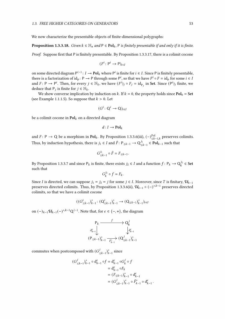
1.3. FREE HIGHER CATEGORIES ON GENERATORS 53

We now characterize the presentable objects of �nite-dimensional polygraphs:

Proposition 1.3.3.18. Given : ∈ N= and P ∈ Pol: , P is �nitely presentable if and only if it is �nite.

Proof. Suppose �rst that P is �nitely presentable. By Proposition 1.3.3.17, there is a colimit cocone

(� 8 : P8 → P)8∈�

on some directed diagram P(−) : � → Pol: where P8 is �nite for 8 ∈ � . Since P is �nitely presentable,there is a factorization of idP : P→ P through some P8 , so that we have � 8 ◦ � = idP for some 8 ∈ �and � : P → P8 . Then, for every 9 ∈ N: , we have (� 8)9 ◦ � 9 = idP9 in Set. Since (P8)9 �nite, wededuce that P9 is �nite for 9 ∈ N: .

We show converse implication by induction on : . If : = 0, the property holds since Pol0 = Set(see Example 1.1.1.5). So suppose that : > 0. Let

(�8 : Q8 → Q)8∈�

be a colimit cocone in Pol: on a directed diagram

3 : � → Pol:

and � : P → Q be a morphism in Pol: . By Proposition 1.3.3.6(iii), (−)Pol≤:−1,: preserves colimits.

Thus, by induction hypothesis, there is 91 ∈ � and � : P≤:−1 → Q 91≤:−1 ∈ Pol:−1 such that

�91≤:−1 ◦ � = �≤:−1.

By Proposition 1.3.3.7 and since P: is �nite, there exists 92 ∈ � and a function 5 : P: → Q 92:∈ Set

such that�92:◦ 5 = �: .

Since � is directed, we can suppose 91 = 92 = 9 for some 9 ∈ � . Moreover, since ) is �nitary,U:−1preserves directed colimits. Thus, by Proposition 1.3.3.6(ii), U:−1 ◦ (−)∗,:−1 preserves directedcolimits, so that we have a colimit cocone

((�8≤:−1)∗:−1 : (Q8

≤:−1)∗:−1 → (Q≤:−1)∗:−1)8∈�

on (−):−1U:−1(−)∗,:−1Q (−) . Note that, for n ∈ {−, +}, the diagram

P: Q 9

:

(P≤:−1)∗:−1 (Q 9

≤:−1)∗:−1

dn:−1

5

dn:−1

� ∗:−1

commutes when postcomposed with (� 9

≤:−1)∗:−1 since

(� 9

≤:−1)∗:−1 ◦ dn

:−1 ◦5 = dn:−1 ◦�

9

:◦ 5

= dn:−1 ◦�:

= (�≤:−1)∗:−1 ◦ dn:−1

= (� 9

≤:−1)∗:−1 ◦ �

∗:−1 ◦ dn

:−1 .

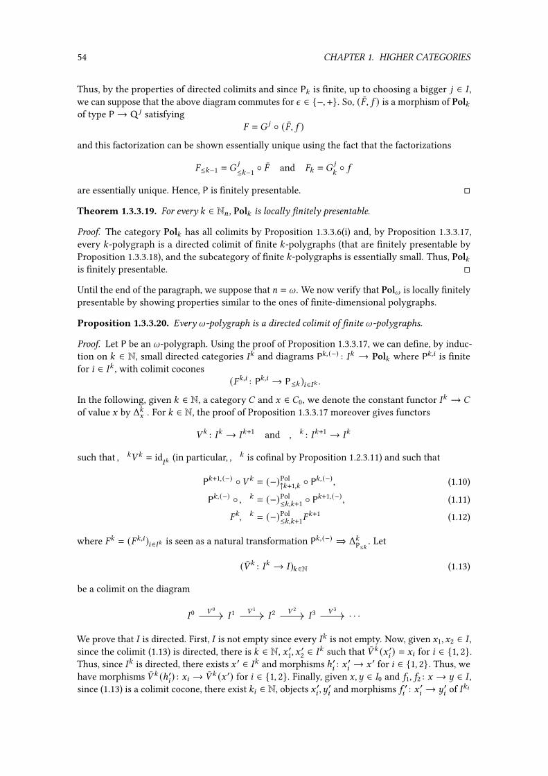
54 CHAPTER 1. HIGHER CATEGORIES

Thus, by the properties of directed colimits and since P: is �nite, up to choosing a bigger 9 ∈ � ,we can suppose that the above diagram commutes for n ∈ {−, +}. So, (� , 5 ) is a morphism of Pol:of type P→ Q 9 satisfying

� = � 9 ◦ (� , 5 )

and this factorization can be shown essentially unique using the fact that the factorizations

�≤:−1 = �9

≤:−1 ◦ � and �: = �9

:◦ 5

are essentially unique. Hence, P is �nitely presentable. �

Theorem 1.3.3.19. For every : ∈ N= , Pol: is locally �nitely presentable.

Proof. The category Pol: has all colimits by Proposition 1.3.3.6(i) and, by Proposition 1.3.3.17,every :-polygraph is a directed colimit of �nite :-polygraphs (that are �nitely presentable byProposition 1.3.3.18), and the subcategory of �nite :-polygraphs is essentially small. Thus, Pol:is �nitely presentable. �

Until the end of the paragraph, we suppose that = = l . We now verify that Poll is locally �nitelypresentable by showing properties similar to the ones of �nite-dimensional polygraphs.

Proposition 1.3.3.20. Every l-polygraph is a directed colimit of �nite l-polygraphs.

Proof. Let P be an l-polygraph. Using the proof of Proposition 1.3.3.17, we can de�ne, by induc-tion on : ∈ N, small directed categories �: and diagrams P:,(−) : �: → Pol: where P:,8 is �nitefor 8 ∈ �: , with colimit cocones

(�:,8 : P:,8 → P≤: )8∈�: .

In the following, given : ∈ N, a category � and G ∈ �0, we denote the constant functor �: → �

of value G by Δ:G . For : ∈ N, the proof of Proposition 1.3.3.17 moreover gives functors

+ : : �: → �:+1 and , : : �:+1 → �:

such that, :+ : = id�:

(in particular,, : is co�nal by Proposition 1.2.3.11) and such that

P:+1,(−) ◦+ : = (−)Pol↑:+1,: ◦ P

:,(−) , (1.10)

P:,(−) ◦, : = (−)Pol≤:,:+1 ◦ P

:+1,(−) , (1.11)

�:, : = (−)Pol≤:,:+1�

:+1 (1.12)

where �: = (�:,8)8∈�: is seen as a natural transformation P:,(−) ⇒ Δ:P≤: . Let

(+ : : �: → � ):∈N (1.13)

be a colimit on the diagram

� 0 � 1 � 2 � 3 · · ·+ 0 + 1 + 2 + 3

We prove that � is directed. First, � is not empty since every �: is not empty. Now, given G1, G2 ∈ � ,since the colimit (1.13) is directed, there is : ∈ N, G ′1, G

′2 ∈ �: such that + : (G ′8 ) = G8 for 8 ∈ {1, 2}.

Thus, since �: is directed, there exists G ′ ∈ �: and morphisms ℎ′8 : G ′8 → G ′ for 8 ∈ {1, 2}. Thus, wehave morphisms + : (ℎ′8 ) : G8 → + : (G ′) for 8 ∈ {1, 2}. Finally, given G,~ ∈ �0 and 51, 52 : G → ~ ∈ � ,since (1.13) is a colimit cocone, there exist :8 ∈ N, objects G ′8 , ~

′8 and morphisms 5 ′8 : G ′8 → ~ ′8 of �:8

1.3. FREE HIGHER CATEGORIES ON GENERATORS 55

such that + :8 (5 ′8 ) = 58 for 8 ∈ {1, 2}. Since (1.13) is directed, we can suppose that :1 = :2, G ′1 = G′2

and ~ ′1 = ~′2. Thus, since �:1 is directed, we have 5 ′1 = 5 ′2 , so that 51 = 52. Hence, � is directed.

For : ∈ N, we de�ne a functor , : : � → �: using the colimit (1.13) as the unique functor suchthat

, : ◦ + ; =, : ◦ · · · ◦, ;−1

for ; ∈ N with ; ≥ : . In particular, we have , : ◦ + : = id�:

, so that , : is co�nal by Proposi-tion 1.2.3.11).

In the following, given : ∈ N and ; ∈ {: + 1, l}, we write n:,; for the counit of the adjunction

(−)Pol↑;,: a (−)

Pol≤:,;

given by Proposition 1.3.3.6(iii) and Proposition 1.3.3.12. Then, given : ∈ N, the cocone �: inducesanother cocone

(�:,8 : (P:,8)↑l → P)8∈�:

on the diagram (−)Pol↑l,: ◦ P

:,(−) , where

�: = (n:,lΔ:P) ◦ ((−)Pol↑l,:�

: ).

By (1.10), we have(−)Pol↑l,:+1 ◦ P

:+1,(−) ◦+ : = (−)Pol↑l,: ◦ P

:,(−)

so that, by the colimit (1.13), there exists a unique functor P(−) : � → Poll such that, for : ∈ N,

P(−) ◦ + : = (−)Pol↑l,: ◦ P

:,(−) .

In particular, since P:,8 is �nite for : ∈ N and 8 ∈ �: , we have that P8 is a �nite l-polygraphfor 8 ∈ � . Given a category � and G ∈ �0, we write ΔG for the constant functor � → Poll ofvalue G . For : ∈ N, we compute that

�:+1+ : = (n:+1,lΔ:+1P + : ) ◦ ((−)Pol↑l,:+1�

:+1+ : )

= (n:+1,lΔ:P) ◦ ((−)Pol↑l,:+1�

:+1+ : ) ◦ ((−)Pol↑l,:+1n

:,:+1(−)Pol↑:+1,: ◦ P

:,(−) )

(by (1.10) and since m−1 (�:+1) = P:+1,(−) and n:,:+1(−)Pol↑:+1,: = id(−)Pol

↑:+1,:)

= (n:+1,lΔ:P) ◦ ((−)Pol↑l,:+1n

:,:+1(−)Pol≤:+1,lΔ

:P) ◦ ((−)

Pol↑l,: (−)

Pol≤:,:+1�

:+1+ : )(by naturality)

= (n:,lΔ:P) ◦ ((−)Pol↑l,:�

:, :+ : )

(since n:+1,l ◦ ((−)Pol↑l,:+1n

:,:+1(−)Pol≤:+1,l ) = n

:,l )

= (n:,lΔ:P) ◦ ((−)Pol↑l,:�

: )

= �: .

Thus, by the colimit (1.13), there exists a unique cocone � : P(−) ⇒ ΔP such that, for : ∈ N,

�+ : = �: .

56 CHAPTER 1. HIGHER CATEGORIES

We verify that it is a colimit cocone. For :, ; ∈ N with : ≤ ; , we have

(−)Pol≤:,l �+

; = (−)Pol≤:,l �

;

= ((−)Pol≤:,ln

;,lΔ;P) ◦ ((−)Pol≤:,l (−)

Pol↑l,;�

; )

= (−)Pol≤:,;�

; (since (−)Pol≤;,ln

;,l = id(−)Pol≤;,l

)

= �:, : · · ·, ;−1 (by (1.12))

= �:, :+ ;

so that, by the colimit (1.13), we have (−)Pol≤:,l � = �:, : for every : ∈ N. Since �: is a colimit

cocone and , : is co�nal,(−)Pol≤:,l � : (−)Pol

≤:,lP(−) ⇒ ΔP≤:

is a colimit cocone by Proposition 1.2.3.10. Since Poll is cocomplete by Proposition 1.3.3.15,and (−)Pol

≤:,l preserves colimits by Proposition 1.3.3.12 for every : ∈ N, and the functors (−)Pol≤l,;

are jointly conservative for ; ∈ N, the latters jointly re�ects colimits. Thus, � : P(−) ⇒ ΔP is acolimit cocone. Hence, P is a directed colimit of �nite l-polygraphs. �

Proposition 1.3.3.21. Given P ∈ Poll , P is �nitely presentable if and only if it is �nite.

Proof. The proof of the �rst implication is similar to the one of Proposition 1.3.3.18. So supposethat P is �nite. Let

(� 8 : Q8 → Q)8∈�be a directed colimit on a diagram Q (−) : � → Poll . Since P is �nite, P = P↑l for some : ∈ N and:-polygraph P. Then, since there is an adjunction (−)Pol

↑l,: a (−)Pol≤:,l by Proposition 1.3.3.12, we

have an isomorphismPoll (P,Q) ' Pol: (P,Q≤: )

Since (−)Pol≤:,l is a left adjoint by Proposition 1.3.3.12,

(� 8≤: : Q8≤: → Q≤: )8∈�

is a directed colimit on (−)Pol≤:,l ◦ Q

(−) . By Proposition 1.3.3.18, since P is �nite, we have anisomorphism

Pol: (P,Q≤: ) ' colim8∈�

Pol: (P,Q8≤: )

and, by the properties of the adjunction (−)Pol↑l,: a (−)

Pol≤:,l , we have

colim8∈�

Pol: (P,Q8≤: ) ' colim

8∈�Poll (P,Q8).

Hence, P is �nitely presentable. �

We can conclude that:

Theorem 1.3.3.22. The category Poll is locally �nitely presentable.

Proof. It has all colimits by Proposition 1.3.3.15. Moreover, every l-polygraph can be writtenas a directed colimit of �nite l-polygraphs by Proposition 1.3.3.20, that are �nitely presentableby Proposition 1.3.3.21. Finally, it is clear that the full subcategory of �nite l-polygraphs isessentially small. Hence, Poll is locally �nitely presentable. �

1.4. STRICT CATEGORIES AND PRECATEGORIES 57

1.4 Strict categories and precategories

In this section, we introduce the de�nitions for the two principal notions of higher categoriesthat we will encounter in the following chapters: strict categories and precategories. Starting fromtheir equational de�nitions, we show that they �t in Batanin’s framework of “higher categoriesas globular algebras” developed in the previous sections. More precisely, we prove that boththeories are associated with truncable monads on globular sets using the criterions proved inthe previous sections (Theorem 1.2.3.20 and Theorem 1.2.4.11). This allows us to derive a notionof polygraph for both. Finally, we recall from Makkai [Mak05] the relation between the twostructures and show how strict categories can be described as precategories which satisfy someexchange condition (Section 1.4.3).

1.4.1 Strict categories

Strict categories, as their name suggests, are a classical example of a theory for higher categoriesthat lies on the strict side of the strict/weak spectrum of higher categories. As such, they do notrepresent faithfully the homotopical information of topological spaces (see [Sim98] or [Ber99]).Nevertheless, they admit a relatively simpler axiomatization than weak higher categories, andcan be encountered in several situations of interest. Below, we recall their equational de�nition,show that they are globular algebras associated with a truncable monad, and derive the associatednotion of polygraph for them.

1.4.1.1 — Equational de�nition. Given = ∈ N ∪ {l}, a strict =-category (�, m−, m+, id, ∗) (oftensimply denoted �) is an =-globular set (�, m−, m+) together with, for : ∈ N with : < =, identityoperations

id:+1 : �: → �:+1

often writen id when there is no ambiguity on : , and, for 8, : ∈ N= with 8 < : , compositionoperations

∗8,: : �: ×8 �: → �:

often denoted ∗8 when there is no ambiguity on : , which satisfy the axioms (S-i) to (S-vi) below.Given :, ; ∈ N= such that : ≤ ; and D ∈ �: , we extend the notations for identity operations andwrite id; (D) for

id; (D) = id; ◦ · · · ◦ id:+1(D)

and, for the sake of conciseness, we often write id;D for id; (D), or even idD when ; = : + 1. Theaxioms are the following:

(S-i) for : ∈ N=−1 and D ∈ �: ,m−:(id:+1D ) = m+: (id

:+1D ) = D,

(S-ii) for 8, : ∈ N= with 8 < : , (D, E) ∈ �: ×8 �: and n ∈ {−, +},

mn:−1(D ∗8 E) =

mn:−1(D) ∗8 m

n:−1(E) if 8 < : − 1,

m−:−1(D) if 8 = : − 1 and n = −,m+:−1(E) if 8 = : − 1 and n = +,

(S-iii) for 8, : ∈ N= such that 8 < : , and D ∈ �: ,

id: (m−8 (D)) ∗8 D = D = D ∗8 id: (m+8 (D)),

58 CHAPTER 1. HIGHER CATEGORIES

(S-iv) for 8, : ∈ N= such that 8 < : , and 8-composable D, E,F ∈ �: ,

(D ∗8 E) ∗8 F = D ∗8 (E ∗8 F),

(S-v) for 8, : ∈ N=−1 such that 8 < : , and (D, E) ∈ �: ×8 �: ,

id:+1(D ∗8 E) = id:+1D ∗8 id:+1E ,

(S-vi) for 8, 9, : ∈ N= such that 8 < 9 < : , and D,D ′, E, E ′ ∈ �: such that D, E are 8-composable,and D,D ′ are 9-composable, and E, E ′ are 9-composable,

(D ∗8 E) ∗9 (D ′ ∗8 E ′) = (D ∗9 D ′) ∗8 (E ∗9 E ′) .

Note that the composition that appear in Axioms (S-iii), (S-iv), (S-v) and (S-vi) are well-de�nedas a consequence of Axioms (S-i) and (S-ii) and the equations satis�ed by the source and targetoperations of a globular set. The Axiom (S-vi) is frequently called the exchange law of strictcategories.Example 1.4.1.2. Given a 2-category � and G,~, I ∈ �0, 51, 52, 53, 61, 62, 63 ∈ �1 and D,D ′, E, E ′ ∈ �2in the following con�guration

G ~ I

51

52

53

61

62

63

⇓D

⇓D ′

⇓E

⇓E ′

we have (D ∗0 E) ∗1 (D ′ ∗0 E ′) = (D ∗1 D ′) ∗0 (E ∗1 E ′) by Axiom (S-vi).Our de�nition of strict categories involves sets, but we could have written a similar de�nitionusing classes to de�ne large strict categories. For such alternative de�nition, we have the followingclassical example:Example 1.4.1.3. There is a large strict 2-category Cat whose 0-cells are the small categories,whose 1-cells are the functors between the 1-categories, and whose 2-cells are the natural trans-formations between functors, and where the operations ∗0,1 is the composition of functors, andthe operations ∗0,2 and ∗1,2 are respectively the horizontal and vertical compositions of naturaltransformations. Note that the exchange law Axiom (S-vi) in this setting corresponds to the usualexchange law for natural transformations.Given two strict =-categories� and � , a morphism � between� and � is the data of an =-globularmorphism � : � → � which moreover satis�es that

– � (id:+1D ) = id:+1� (D) for every : ∈ N=−1 and D ∈ �: ,

– � (D ∗8 E) = � (D) ∗8 � (E) for every 8, : ∈ N= with 8 < : and 8-composable D, E ∈ �: .

We often call such morphisms =-functors. We write Cat= for the category of strict =-categories.

There is a functorU= : Cat= → Glob=

which maps a strict =-category to its underlying =-globular set. The above de�nition of strict=-categories directly translates into an essentially algebraic theory, so that the functor U= isinduced by a morphism between the essentially algebraic theory of =-globular sets (c.f. Re-mark 1.2.2.2) and the one of strict =-categories. Thus, we get:

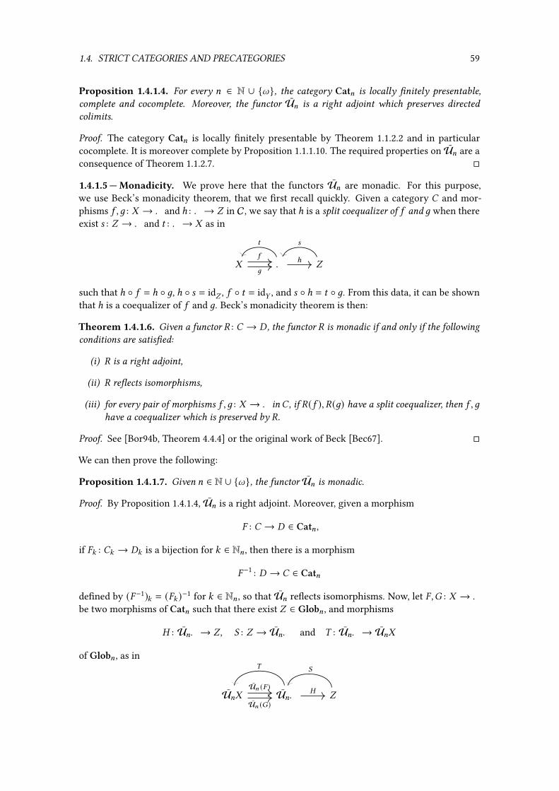
1.4. STRICT CATEGORIES AND PRECATEGORIES 59

Proposition 1.4.1.4. For every = ∈ N ∪ {l}, the category Cat= is locally �nitely presentable,complete and cocomplete. Moreover, the functor U= is a right adjoint which preserves directedcolimits.

Proof. The category Cat= is locally �nitely presentable by Theorem 1.1.2.2 and in particularcocomplete. It is moreover complete by Proposition 1.1.1.10. The required properties on U= are aconsequence of Theorem 1.1.2.7. �

1.4.1.5 — Monadicity. We prove here that the functors U= are monadic. For this purpose,we use Beck’s monadicity theorem, that we �rst recall quickly. Given a category � and mor-phisms 5 , 6 : - → . and ℎ : . → / in C, we say that ℎ is a split coequalizer of 5 and 6 when thereexist B : / → . and C : . → - as in

- . /5

6

ℎ

C B

such that ℎ ◦ 5 = ℎ ◦ 6, ℎ ◦ B = id/ , 5 ◦ C = id. , and B ◦ ℎ = C ◦ 6. From this data, it can be shownthat ℎ is a coequalizer of 5 and 6. Beck’s monadicity theorem is then:

Theorem 1.4.1.6. Given a functor ' : � → � , the functor ' is monadic if and only if the followingconditions are satis�ed:

(i) ' is a right adjoint,

(ii) ' re�ects isomorphisms,

(iii) for every pair of morphisms 5 , 6 : - → . in� , if '(5 ), '(6) have a split coequalizer, then 5 , 6have a coequalizer which is preserved by '.

Proof. See [Bor94b, Theorem 4.4.4] or the original work of Beck [Bec67]. �

We can then prove the following:

Proposition 1.4.1.7. Given = ∈ N ∪ {l}, the functor U= is monadic.

Proof. By Proposition 1.4.1.4, U= is a right adjoint. Moreover, given a morphism

� : � → � ∈ Cat= ,

if �: : �: → �: is a bijection for : ∈ N= , then there is a morphism

�−1 : � → � ∈ Cat=

de�ned by (�−1): = (�: )−1 for : ∈ N= , so that U= re�ects isomorphisms. Now, let �,� : - → .

be two morphisms of Cat= such that there exist / ∈ Glob= , and morphisms

� : U=. → /, ( : / → U=. and ) : U=. → U=-

of Glob= , as in

U=- U=. /U= (� )

U= (�)

�

) (

60 CHAPTER 1. HIGHER CATEGORIES

that witness that U= (� ), U= (�) is a split coequalizer. We prove that �,� has a coequalizer whichis preserved by U= . For this purpose, we shall equip / with a structure of a strict =-category.For 8, : ∈ N= with 8 < : and (D, E) ∈ /: ×8 /: , we put

D ∗8 E = � (( (D) ∗8 ( (E))

and, given : ∈ N=−1 and D ∈ �: , we put

id:+1D = � (id:+1( (D) )

We verify that the axioms of strict =-categories are veri�ed. Let : ∈ N=−1, D ∈ /: and n ∈ {−, +}.We have

mn:(id:+1D ) = mn: (� (id

:+1( (D) ))

= � (mn:(id:+1

( (D) ))= � (( (D)) = D

so that Axiom (S-i) is satis�ed. Now, let 8, : ∈ N= such that 8 < : , (D, E) ∈ /: ×8 /: and n ∈ {−, +}.We have

mn:−1(D ∗8 E) = � (m

n:−1(( (D) ∗8 ( (E)))

=

� (mn

:−1(( (D)) ∗8 mn:−1(( (E))) if 8 < : − 1,

� (m−:−1(( (D))) if 8 = : − 1 and n = −,

� (m+:−1(( (E))) if 8 = : − 1 and n = +,

so that, by reducing the last expressions, we see that Axiom (S-ii) is satis�ed. Now, let 8, : ∈ N=such that 8 < : , and D ∈ /: . We have

id: (m−8 (D)) ∗8 D = � (( (� (id:( (m−

8(D)) )) ∗8 ( (D))

= � (( (� (id:m−8(( (D)) )) ∗8 (�( (D))

= � (�) (id:m−8(( (D)) ) ∗8 �)( (D))

= �� () (id:m−8(( (D)) ) ∗8 )( (D))

= �� () (id:m−8(( (D)) ) ∗8 )( (D))

= � (�) (id:m−8(( (D)) ) ∗8 �)( (D))

= � (id:m−8(( (D)) ∗8 ( (D))

= � (( (D)) = D

and, similarly, D ∗8 id: (m+8 (D)) = D, so that Axiom (S-iii) holds. Now, let 8, : ∈ N= such that 8 < : ,and 8-composable D, E,F ∈ �: . We have

(D ∗8 E) ∗8 F = � (( (� (( (D) ∗8 ( (E))) ∗8 ( (F))= � ((� (( (D) ∗8 ( (E)) ∗8 (�( (F))= � (�) (( (D) ∗8 ( (E)) ∗8 �)( (F))= �� () (( (D) ∗8 ( (E)) ∗8 )( (F))= �� () (( (D) ∗8 ( (E)) ∗8 )( (F))

1.4. STRICT CATEGORIES AND PRECATEGORIES 61

= � (�) (( (D) ∗8 ( (E)) ∗8 �)( (F))= � ((( (D) ∗8 ( (E)) ∗8 ( (F))= � (( (D) ∗8 ( (E) ∗8 ( (F))

and, similarly,D ∗8 (E ∗8F) = � (( (D) ∗8 ( (E) ∗8 ( (F)). So that Axiom (S-iv) is satis�ed. Axioms (S-v)and (S-vi) are proved similarly, so / is equipped with a structure of a strict =-category.

We now verify that � is a strict =-category morphism. Given : ∈ N=−1 and D ∈ .: , we have

id:� (D) = � (id

:(� (D) ) = � (id

:D)

and, given 8, : ∈ N= with 8 < : , and (D, E) ∈ .: ×8 .: , we have

� (D) ∗8 � (E) = � ((� (D) ∗8 (� (E))= � (�) (D) ∗8 �) (E))= �� () (D) ∗8 ) (E))= �� () (D) ∗8 ) (E))= � (�) (D) ∗8 �) (E))= � (D ∗8 E)

so that � is a strict =-category morphism.

We now prove that � is the coequalizer of � and � in Cat= . Let : . →, be an =-functor suchthat � = � . Then, since� is the coequalizer of U= (� ) and U= (�), there is a unique morphism

′ : U=/ → U=,

of Glob= such that ′� = . We are only left to prove that ′ is an =-functor. First, note that wehave

′ = ′�( = ( and (� = �) = �) = .

Now, given : ∈ N=−1 and D ∈ �: , we have

( (id:+1D ) = (� (id:+1( (D) )

= (id:+1( (D) )

= id:+1 ( (D) .

Moreover, given 8, : ∈ N= with 8 < : , and (D, E) ∈ �: ×�: , we have

( (D ∗8 E) = (� (( (D) ∗8 ( (E))= (( (D) ∗8 ( (E))= ( (D) ∗8 ( (E),

so that ′ is an =-functor. Hence, � is the coequalizer in Cat= of � and � . We can concludewith Theorem 1.4.1.6. �

1.4.1.8 — Truncation and inclusion functors. Let :, ; ∈ N ∪ {l} such that : < ; . There is atruncation functor

(−)Cat≤:,; : Cat; → Cat:

which maps a strict ;-category � to its evident underlying strict :-category, denoted �≤: , andcalled the :-truncation of � .

62 CHAPTER 1. HIGHER CATEGORIES

Conversely, there is an inclusion functor

(−)Cat↑;,: : Cat: → Cat;

which maps a strict :-category� to the strict ;-category�↑; , called the ;-inclusion of� , and de�nedby

(�↑; )≤: = � and (�↑; )< = �:

for< ∈ N; with : < <, and such that

– for< ∈ N;−1 with : ≤ < and D ∈ (�↑; )<+1, m−< (D) = m+< (D) = D,

– for< ∈ N;−1 with : ≤ < and D ∈ (�↑; )< , id<+1D = D,

– for 8,< ∈ N; with 8 < : < < and (D, E) ∈ (�↑; )< ×8 (�↑; )< , D ∗8,< E = D ∗8,: E ,

– for 8,< ∈ N; with : ≤ 8 < < and (D, E) ∈ (�↑; )< ×8 (�↑; )< , D ∗8,< E = D = E .

There is an adjunction (−)Cat↑;,: a (−)

Cat≤:,; whose unit is the identity and whose counit i:,; is such

that, given a strict ;-category � , the ;-functor i:,;�

: (�≤: )↑; → � is de�ned by (i:,;�)≤: = id�≤: and,

for< ∈ N; with< > : , i:,;�

maps D ∈ ((�≤: )↑; )< = �: to id<D .

1.4.1.9 — Globular algebras. By Proposition 1.4.1.4, each functor U= admits a left adjoint F=for = ∈ N ∪ {l}. In particular, the adjunction Fl a Ul de�nes a monad (), [, `), which is�nitary by Proposition 1.4.1.4, and it induces categories of algebras Alg= for = ∈ N ∪ {l} asexplained in Section 1.2.3. By Proposition 1.4.1.7, the comparison functor �l : Catl → Alglis an equivalence of categories, that moreover satis�es that Ul�l = Ul . Using the criterionintroduced in Paragraph 1.2.3.13, we prove that the other categories Cat= are, up to equivalence,the categories of algebras Alg= :

Theorem 1.4.1.10. For every = ∈ N, there exists an equivalence

�= : Cat= → Alg=

making the following diagram commute

Catl Algl

Cat= Alg=

�l

(−)Cat≤= (−)Alg

≤=

�=

and such thatU=�= = U= . Moreover, we have a commutative diagram

Cat=+1 Alg=+1

Cat= Alg=

�=+1

(−)Cat≤= (−)Alg

≤=

�=.

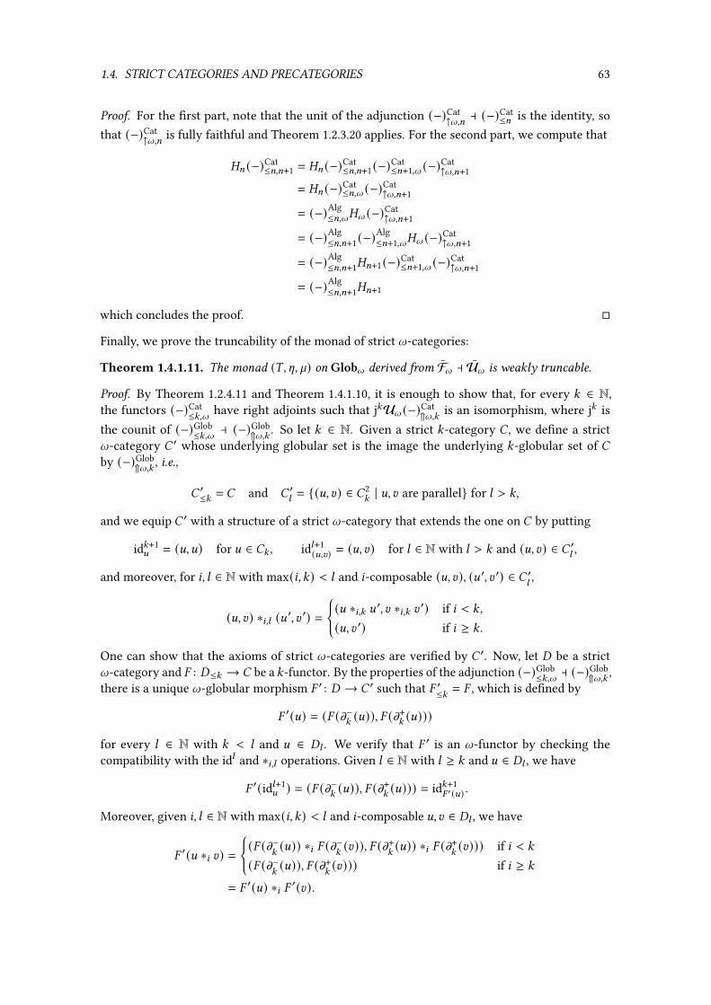
1.4. STRICT CATEGORIES AND PRECATEGORIES 63

Proof. For the �rst part, note that the unit of the adjunction (−)Cat↑l,= a (−)

Cat≤= is the identity, so

that (−)Cat↑l,= is fully faithful and Theorem 1.2.3.20 applies. For the second part, we compute that

�= (−)Cat≤=,=+1 = �= (−)Cat

≤=,=+1(−)Cat≤=+1,l (−)Cat

↑l,=+1

= �= (−)Cat≤=,l (−)Cat

↑l,=+1

= (−)Alg≤=,l�l (−)Cat

↑l,=+1

= (−)Alg≤=,=+1(−)

Alg≤=+1,l�l (−)

Cat↑l,=+1

= (−)Alg≤=,=+1�=+1(−)

Cat≤=+1,l (−)Cat

↑l,=+1

= (−)Alg≤=,=+1�=+1

which concludes the proof. �

Finally, we prove the truncability of the monad of strict l-categories:

Theorem 1.4.1.11. The monad (), [, `) on Globl derived from Fl a Ul is weakly truncable.

Proof. By Theorem 1.2.4.11 and Theorem 1.4.1.10, it is enough to show that, for every : ∈ N,the functors (−)Cat

≤:,l have right adjoints such that j:Ul (−)Cat⇑l,: is an isomorphism, where j: is

the counit of (−)Glob≤:,l a (−)

Glob⇑l,: . So let : ∈ N. Given a strict :-category � , we de�ne a strict

l-category � ′ whose underlying globular set is the image the underlying :-globular set of �by (−)Glob

⇑l,: , i.e.,

� ′≤: = � and � ′;= {(D, E) ∈ �2

:| D, E are parallel} for ; > :,

and we equip � ′ with a structure of a strict l-category that extends the one on � by putting

id:+1D = (D,D) for D ∈ �: , id;+1(D,E) = (D, E) for ; ∈ N with ; > : and (D, E) ∈ � ′;,

and moreover, for 8, ; ∈ N with max(8, :) < ; and 8-composable (D, E), (D ′, E ′) ∈ � ′;,

(D, E) ∗8,; (D ′, E ′) ={(D ∗8,: D ′, E ∗8,: E ′) if 8 < : ,(D, E ′) if 8 ≥ : .

One can show that the axioms of strict l-categories are veri�ed by � ′. Now, let � be a strictl-category and � : �≤: → � be a :-functor. By the properties of the adjunction (−)Glob

≤:,l a (−)Glob⇑l,: ,

there is a unique l-globular morphism � ′ : � → � ′ such that � ′≤: = � , which is de�ned by

� ′(D) = (� (m−:(D)), � (m+

:(D)))

for every ; ∈ N with : < ; and D ∈ �; . We verify that � ′ is an l-functor by checking thecompatibility with the id; and ∗8,; operations. Given ; ∈ N with ; ≥ : and D ∈ �; , we have

� ′(id;+1D ) = (� (m−: (D)), � (m+:(D))) = id:+1

� ′ (D) .

Moreover, given 8, ; ∈ N with max(8, :) < ; and 8-composable D, E ∈ �; , we have

� ′(D ∗8 E) ={(� (m−

:(D)) ∗8 � (m−: (E)), � (m

+:(D)) ∗8 � (m+: (E))) if 8 < :

(� (m−:(D)), � (m+

:(E))) if 8 ≥ :

= � ′(D) ∗8 � ′(E).

64 CHAPTER 1. HIGHER CATEGORIES

Thus, � ′ is an l-functor. Hence, the natural bijective correspondence

(−)Glob≤:,l : Globl (�,� ′) → Glob: (�≤: ,�)

restricts to a bijective correspondence

(−)Cat≤:,l : Catl (�,� ′) → Cat: (�≤: ,�)

so that the operation � ↦→ � ′ extends to a functor (−)Cat⇑l,: which is right adjoint to (−)Cat

≤:,l .Moreover, by the de�nition of � ′ above, the natural morphism j:Ul (−)Cat

⇑l,: is an isomorphism.Hence, Theorem 1.2.4.11 applies and (), [, `) is a weakly truncable monad. �

Remark 1.4.1.12. We highlight that the criterions given by Theorem 1.2.3.20 and Theorem 1.2.4.11enabled us to prove that the categories Cat= are globular algebras derived from a truncable monadon Globl without giving an explicit description of this monad, which could have been a tediousexercise [Pen99].

1.4.1.13 — Free constructions. Using Theorem 1.4.1.10 and Theorem 1.4.1.11, we can instantiatethe de�nitions and properties developed in Section 1.3 to de�ne free constructions on strict =-cate-gories. In particular, for every = ∈ N, there is a notion of =-cellular extension, with associatedcategory Cat+= de�ned like Alg+= . Moreover, there is a canonical forgetful functor Cat=+1 → Cat+=which has a left adjoint

−[−]= : Cat+= → Cat=+1

which can be chosen such that � [- ]≤= = � for (�,- ) ∈ Cat+= . As was shown in [Mét08], the(=+1)-cells of a free extension admit a syntactical description consisting of “well-typed” termsconsidered up to the axioms of strict categories (c.f. Paragraph 1.4.1.1). We shall give a moreprecise de�nition of “well-typed” in Section 2.4 when we introduce the exact formulation of theword problem for strict categories. Up to this de�nition, the result of Métayer is the following:

Proposition 1.4.1.14 ([Mét08]). Given (�,- ) ∈ Cat+= , the set� [- ]=+1 is the quotient by the axiomsof (=+1)-categories of the “well-typed” subset of terms de�ned inductively as follows:

– given 6 ∈ - , there is a term gen(6),

– given D ∈ �= , there is a term id=+1= (D),

– given 8 ∈ N= and two terms C1, C2, there is a term C1 ∗8 C2.

Remark 1.4.1.15. In the above property, id=+1= and ∗8 are syntactical symbols which represent theoperations id=+1= and ∗8 of a strict category.Using the functors −[−]: , we can de�ne, for every = ∈ N ∪ {l}, a notion of =-polygraph withassociated category Pol= , and a functor

(−)∗,= : Pol= → Cat=

which maps an =-polygraph P to the free strict =-category P∗ induced by the generators containedin P. Note that, when = > 0, as a consequence of the compatibility of −[−]=−1 with truncation, theunderlying strict (=−1)-category (P∗)≤=−1 of P∗ is exactly (P≤=−1)∗. Proposition 1.4.1.14 extendsto a syntactical description of the cells of free categories on polygraphs:

Proposition 1.4.1.16. Given an =-polygraph P and : ∈ N= , the set P∗: of :-cells of P∗ is the quotient

by the axioms of :-categories of the “well-typed” subset of :-terms where

1.4. STRICT CATEGORIES AND PRECATEGORIES 65

– given : ∈ N= and 6 ∈ P: , there is a :-term gen: (6),

– given : ∈ N=−1 and a :-term C , there is a (:+1)-term id:+1:(D),

– given 8, : ∈ N= with 8 < : and two :-terms C1, C2, there is a :-term C1 ∗8 C2.

Remark 1.4.1.17. In particular, given an =-polygraph P, every cell of P∗ can be written as a �niteexpression involving identity and composition operations on generators of P.Example 1.4.1.18. Given the 1-polygraph P with P0 = {G} and P1 = {5 : G → G}, the strict1-category P∗ is the monoid of natural numbers (N, 0, +).Example 1.4.1.19. We de�ne a 3-polygraph P that aims at encoding the structure of a pseudomonoidin a 2-monoidal category as follows. We put

P0 = {G} P1 = {1 : G → G} P2 = {` : 2⇒ 1, [ : 0⇒ 1}

where, given = ∈ N, we write = for the composite 1 ∗0 · · · ∗0 1 of = copies of 1, and we de�ne P3as the set with the following three elements

L : ([ ∗0 id21) ∗1 ` V id2

1R : (id2

1 ∗0 [) ∗1 ` V id21

A : (` ∗0 id21) ∗1 ` V (id2

1 ∗0 `) ∗1 ` .

It is convenient to represent the 2-cells of P∗ using string diagrams. In this representation, the2-generators [ and ` are represented by and respectively, and the 2-cells of the form id2

= arerepresented by sequences of = wires for = ∈ N. Moreover, given D, E ∈ P∗2, when D, E are0-composable (resp. 1-composable), a representation of the 2-cell D ∗0 E (resp. D ∗1 E) is obtainedby concatenating horizontally (resp. vertically) representations of D and E . For example, usingthis representation, the 3-generators L, R and A, can be pictured by

L : V

R : V

A : V .

Note that, by Axiom (S-vi), a 2-cell can admit several representations as string diagrams. Forexample, the 2-cell

` ∗0 id23 ∗0 ` = (` ∗0 id2

5) ∗1 (id24 ∗0 `) = (id

25 ∗0 `) ∗1 (` ∗0 id2

4)

can be represented by the three string diagrams

and and .

1.4.2 Precategories

We now introduce precategories. They can be described, in a sense that will be made precisein Section 1.4.3, as “strict categories without exchange law” and generalize in higher dimensionsthe 2-dimensional theory of sesquicategories de�ned by Street in [Str96]. The absence of ex-change makes precategories more amenable to computational treatment than strict categories, aswitnessed by their use as the underlying structure of the Globular proof assistant [BV17; BKV16].Following this observation, in the coming chapters, we will use precategories as a better syntacticrepresentation of strict categories introduced Chapter 2, and as the underlying structure of anextension of rewriting theory to Gray categories in Chapter 4. Below, like for strict categories,we introduce their equational de�nition, show that they are the globular algebras of a truncablemonad on globular sets, and derive the associated notion of polygraph for them.

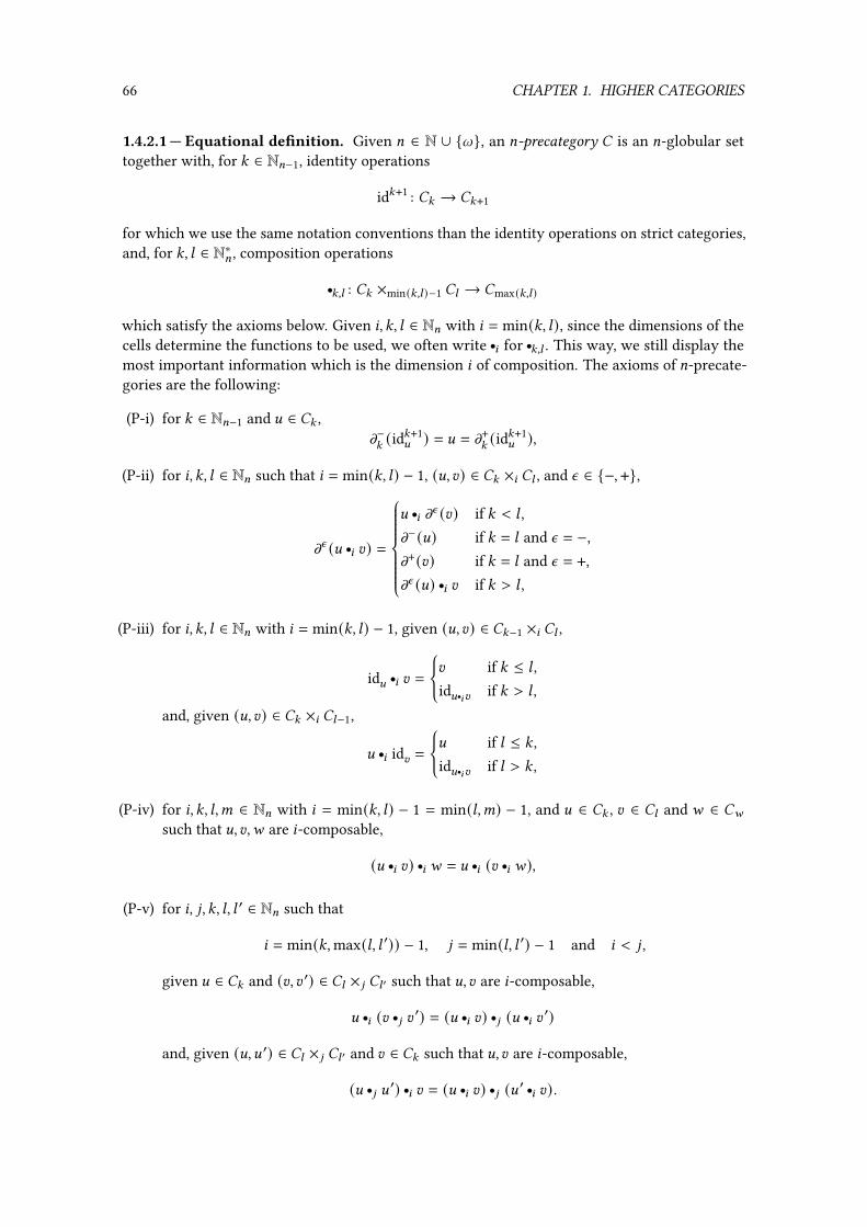
66 CHAPTER 1. HIGHER CATEGORIES

1.4.2.1 — Equational de�nition. Given = ∈ N ∪ {l}, an =-precategory � is an =-globular settogether with, for : ∈ N=−1, identity operations

id:+1 : �: → �:+1

for which we use the same notation conventions than the identity operations on strict categories,and, for :, ; ∈ N∗= , composition operations

r:,; : �: ×min(:,;)−1 �; → �max(:,;)

which satisfy the axioms below. Given 8, :, ; ∈ N= with 8 = min(:, ;), since the dimensions of thecells determine the functions to be used, we often write r

8 for r:,; . This way, we still display the

most important information which is the dimension 8 of composition. The axioms of =-precate-gories are the following:

(P-i) for : ∈ N=−1 and D ∈ �: ,m−:(id:+1D ) = D = m+

:(id:+1D ),

(P-ii) for 8, :, ; ∈ N= such that 8 = min(:, ;) − 1, (D, E) ∈ �: ×8 �; , and n ∈ {−, +},

mn (D r8 E) =

D r

8 mn (E) if : < ; ,

m−(D) if : = ; and n = −,m+(E) if : = ; and n = +,mn (D) r8 E if : > ; ,

(P-iii) for 8, :, ; ∈ N= with 8 = min(:, ;) − 1, given (D, E) ∈ �:−1 ×8 �; ,

idD r8 E =

{E if : ≤ ; ,idD q8E if : > ; ,

and, given (D, E) ∈ �: ×8 �;−1,

D r8 idE =

{D if ; ≤ : ,idD q8E if ; > : ,

(P-iv) for 8, :, ;,< ∈ N= with 8 = min(:, ;) − 1 = min(;,<) − 1, and D ∈ �: , E ∈ �; and F ∈ �Fsuch that D, E,F are 8-composable,

(D r8 E) r8 F = D r

8 (E r8 F),

(P-v) for 8, 9, :, ;, ; ′ ∈ N= such that

8 = min(:,max(;, ; ′)) − 1, 9 = min(;, ; ′) − 1 and 8 < 9 ,

given D ∈ �: and (E, E ′) ∈ �; ×9 �; ′ such that D, E are 8-composable,

D r8 (E r

9 E′) = (D r

8 E) r9 (D r8 E′)

and, given (D,D ′) ∈ �; ×9 �; ′ and E ∈ �: such that D, E are 8-composable,

(D r9 D′) r8 E = (D r

8 E) r9 (D ′ r8 E).

1.4. STRICT CATEGORIES AND PRECATEGORIES 67

Remark 1.4.2.2. Provided that the Axioms (P-i) to (P-iv) are satis�ed, Axiom (P-v) can be shownequivalent to the more symmetrical axiom

(P-v)’ for every 8, 9, : ∈ N= satisfying 8 < 9 < : , and cells D1, D2 ∈ �8+1, E1, E2 ∈ � 9+1 and F ∈ �:such that D1,F,D2 are 8-composable and E1,F, E2 are 9-composable, we have

D1 r8 (E1 r

9 F r9 E2) r8 D2 = (D1 r

8 E1 r8 D2) r9 (D1 r

8 F r8 D2) r9 (D1 r

8 E2 r8 D2).

Example 1.4.2.3. Given a 2-precategory � with two 2-cells q andk as in

G ~ I

5

5 ′

6

6′

⇓ q ⇓ k

there are two ways to compose q andk together, given by

(q r0 6) r1 (5 ′ r0 k ) and (5 r0 k ) r1 (q r0 6′)that can be represented using string diagrams by

5 6

q

k

5 ′ 6′

and

5 6

q

k

5 ′ 6′

and these two composites are not expected to be equal in � . Moreover, by our de�nition ofprecategories, there is no such thing as a valid cell q r0 k , and the string diagram

5 6

q k

5 ′ 6′

makes no sense in this setting.Given two =-precategories � and � , a morphism of =-precategories between � and � (also called=-prefunctor), is a morphism of =-globular sets � : � → � such that

– � (id:+1D ) = id:+1� (D) for : ∈ N=−1 and D ∈ �: ,

– � (D r8 E) = � (D) r8 � (E) for 8, :, ; ∈ N= with 8 = min(:, ;) − 1 and (D, E) ∈ �: ×8 �; .

We write PCat= for the category of =-precategories.

There is a functorU= : PCat= → Glob=

which maps an =-precategory to its underlying =-globular set. Like for strict categories, the abovede�nition of =-precategories directly translates into an essentially algebraic theory, so that thefunctor U= is induced by a morphism between the essentially algebraic theory of =-globular sets(c.f. Remark 1.2.2.2) and the one of =-precategories. Thus:

68 CHAPTER 1. HIGHER CATEGORIES

Proposition 1.4.2.4. The category PCat= is locally �nitely presentable, complete and cocomplete.Moreover, the functor U= is a right adjoint which preserves directed colimits.

Proof. This is a consequence of Theorem 1.1.2.2, Proposition 1.1.1.10 and Theorem 1.1.2.7. �

Like for strict categories, the functor U= can be shown monadic using the monadicity theorem:

Proposition 1.4.2.5. For every = ∈ N ∪ {l}, the functor U= is monadic.

Proof. By a direct adaptation of Proposition 1.4.2.5. �

1.4.2.6 — Truncation and inclusion functors. Let :, ; ∈ N ∪ {l} such that : < ; . There is a:-truncation functor

(−)PCat≤:,; : PCat; → PCat:

which maps an ;-precategory � to its evident underlying :-precategory, denoted �≤: , called the:-truncation of � .

Conversely, there is an ;-inclusion functor

(−)PCat↑;,: : Cat: → Cat;

which maps a :-precategory� to the ;-precategory�↑; , called the ;-inclusion of� , and de�ned by

(�↑; )≤: = � and (�↑; )< = �:

for< ∈ N; with : < < and such that

– for< ∈ N;−1 with : ≤ < and D ∈ (�↑; )<+1, m−< (D) = m+< (D) = D,

– for< ∈ N;−1 with : ≤ < and D ∈ (�↑; )< , id<+1D = D,

– for 8,<,<′ ∈ N; with 8 = min(<,<′) − 1 < : and (D, E) ∈ (�↑; )< ×8 (�↑; )<′ ,

D r<,<′ E = D rmin(<,:),min(<′,:) E ,

– for 8,<,<′ ∈ N; with : ≤ 8 = min(<,<′) − 1 and (D, E) ∈ �< ×8 �< ,

D r<,<′ E = D = E .

There is an adjunction (−)PCat↑;,: a (−)

PCat≤:,; whose unit is the identity and whose counit i:,; is such

that, given an ;-precategory � , the ;-functor i:,;�

: (�≤: )↑; → � is de�ned by (i:,;�)≤: = id�≤: and,

for< ∈ N; with< > : , i:,;�

maps D ∈ ((�≤: )↑; )< = �: to id<D .

1.4.2.7 — Globular algebras. By Proposition 1.4.1.4, each functor U= admits a left adjoint F=for = ∈ N ∪ {l}. In particular, the adjunction Fl a Ul de�nes a monad (), [, `), which is�nitary by Proposition 1.4.1.4, and it induces categories of algebras Alg= for = ∈ N ∪ {l}. ByProposition 1.4.1.7, the comparison functor �l : PCatl → Algl is an equivalence of categories,that moreover satis�es thatUl�l = Ul . By adapting the proof of Theorem 1.4.1.10, we obtainan equivalent statement for precategories:

1.4. STRICT CATEGORIES AND PRECATEGORIES 69

Theorem 1.4.2.8. For every = ∈ N, there exists an equivalence

�= : PCat= → Alg=

making the following diagram commute

PCatl Algl

PCat= Alg=

�l

(−)PCat≤= (−)Alg

≤=

�=

and such thatU=�= = U= . Moreover, we have a commutative diagram

PCat=+1 Alg=+1

PCat= Alg=

�=+1

(−)PCat≤= (−)Alg

≤=

�=.

Finally, by a direct adaptation of the proof of Theorem 1.4.1.11, we obtain the truncability of themonad for precategories:

Theorem 1.4.2.9. The monad (), [, `) derived from Fl a Ul is weakly truncable.

1.4.2.10 — Free constructions. Like for strict categories, using Theorem 1.4.2.8 and Theo-rem 1.4.2.9, we can instantiate the constructions and properties developed in Section 1.3 to de�nefree constructions on =-precategories. In particular, for every = ∈ N, there is a notion of =-cellularextension for strict =-precategories, with associated category PCat+= de�ned like Alg+= . Moreover,the canonical forgetful functor PCat=+1 → PCat+= has a left adjoint

−[−]= : PCat+= → PCat=+1

which can be chosen such that � [- ]≤= = � for (�,- ) ∈ PCat+= .Using the functors −[−]: , we can de�ne, for every = ∈ N ∪ {l}, a notion of =-polygraph for

precategories, called =-prepolygraph, with associated category PPol= , and a functor

(−)∗,= : PPol= → PCat=

which maps an=-prepolygraph P to the free=-precategory P∗ induced by the generators containedin P. Note that, when = > 0, as a consequence of the compatibility of −[−]=−1 with truncation,the underlying (=−1)-precategory (P∗)≤=−1 of P∗ is exactly (P≤=−1)∗.Remark 1.4.2.11. By adapting the results of Métayer [Mét08], one can obtain analogues of Propo-sition 1.4.1.14 and Proposition 1.4.1.16 for precategories, so that the cells of the free precategorieson cellular extensions and prepolygraphs can be described by “well-typed” terms considered up tothe axioms of precategories given in Paragraph 1.4.2.1. In the case of prepolygraphs, the de�nitionof these terms can be found in Paragraph 4.1.2.7.

Example 1.4.2.12. By adapting the 3-polygraph of Example 1.4.1.19, we de�ne a 3-prepolygraph Pthat aims at encoding the structure of a pseudomonoid in a 2-monoidal precategory as follows.We put

P0 = {G} P1 = {1 : G → G} P2 = {` : 2⇒ 1, [ : 0⇒ 1}

70 CHAPTER 1. HIGHER CATEGORIES

where, given = ∈ N, we write = for the composite 1 ∗0 · · · ∗0 1 of = copies of 1, and we de�ne P3as the set with the following three elements

L : ([ r0 1) r1 ` V id21

R : (1 r0 [) r1 ` V id21

A : (` r0 1) r1 ` V (1 r0 `) r1 `.

Like for Example 1.4.1.19, we can represent the 2-cells of P∗ using string diagrams. In this repre-sentation, the 2-generators [ and ` are represented by and respectively. Moreover, a 2-cellof the form < r0 D r0 = for some <,= ∈ N and D ∈ P∗2 is represented by adding < wires on theleft and = wires on the right of a representation of D. Finally, given 1-composable D, E ∈ P∗2, arepresentation of D r1 E is obtained by concatenating vertically representations of D and E . Forexample, using this representation, the 3-generators L, R and A can be pictured by

L : V

R : V

A : V .

Since precategories do not satisfy any exchange law (unlike strict categories), it can be shownthat the 2-cells of P∗ admit a unique representation as string diagrams (see Theorem 4.1.2.4 andCorollary 4.1.2.5 in Chapter 4). In particular, the two string diagrams

and

represent the di�erent 2-cells

(` r0 5) r1 (4 r0 `) and (5 r0 `) r1 (` r0 4)

of P∗. Note moreover that the diagram

makes no sense in the precategorical setting.

1.4.3 Categories as precategories

In this section, we justify the de�nition of precategories as “strict categories without the exchangelaw” and recall from [Mak05] how strict categories can be expressed as precategories satisfying acondition analogous to the exchange law. This equivalent de�nition will be used in particular inthe next chapterto give an e�ective description of the free extension on an =-cellular extension,ultimately leading to an e�cient algorithm which solves the word problem on polygraphs of strictcategories.

1.4.3.1 — Categories as precategories. For = ∈ N ∪ {l} and � ∈ PCat= , we write (E) for thefollowing property on �:

(E) for 8, :, ; ∈ N= with 1 ≤ 8 = min(:, ;) − 1, D ∈ �: and E ∈ �; , if D, E are (8−1)-com-posable, then

(D r8−1 m

−8 (E)) r8 (m+8 (D) r8−1 E) = (m−8 (D) r8−1 E) r8 (D r

8−1 m+8 (E)).

1.4. STRICT CATEGORIES AND PRECATEGORIES 71

Let PCat(E)= be the full subcategory of PCat= of those =-precategories � that satisfy (E). Thecondition (E) can be thought as an equivalent for precategories of the exchange law (S-vi) ofstrict categories. We now introduce a functor from strict =-categories to =-precategories whichsatisfy (E) with the following proposition:

Proposition 1.4.3.2. Given = ∈ N ∪ {l}, there is a canonical functor Θ= : Cat= → PCat(E)= .

Proof. Given � ∈ Cat= , we de�ne a structure of =-precategory on the underlying =-globularset of � . We keep the identities given by the strict =-category structure and de�ne the com-position operations r(−) on � based on the composition operations ∗(−) . Given 8, :, ; ∈ N=with 8 = min(:, ;) − 1, D ∈ �: and E ∈ �; such that D, E are 8-composable, we put

D r8 E = id<D ∗8 id<E

where < = max(:, ;). Axioms (P-ii), (P-i), (P-iii), (P-iv) are then direct consequences of theaxioms of strict =-categories. We only prove the �rst part of (P-v) since the other is symmet-rical. Let 8, 9, :, ;, ; ′ ∈ N= with 8 = min(:,max(;, ; ′)) − 1, 9 = min(;, ; ′) − 1 and 8 < 9 , D ∈ �: ,and E ∈ �; , E ′ ∈ �; ′ such that D, E are 8-composable and E, E ′ are 9-composable. Writing <for max(;, ; ′), we have

D r8 (E r

9 E′) = id<D ∗8 id< (id<E ∗9 id<E′ ) (by de�nition of r(−) )= id<D ∗8 (id<E ∗9 id<E′ )= (id<D ∗9 id<D ) ∗8 (id<E ∗9 id<E′ ) (by Axiom (S-iii))= (id<D ∗8 id<E ) ∗9 (id<D ∗8 id<E′ ) (by Axiom (S-vi))

= id< (id9+1D ∗8 E) ∗9 id< (id9′+1D ∗8 E ′) (by Axiom (S-v))

= (D r8 E) r9 (D r

8 E′) (by de�nition of r(−) )

which concludes the proof of (P-v). Thus,� is an =-precategory. We now show that it satis�es thecondition (E) above. So let 8, :, ; ∈ N= with 1 ≤ 8 = min(:, ;) − 1, D ∈ �: and E ∈ �; such that D, Eare (8−1)-composable. Writing< for max(:, ;), we have

(D r8−1 m

−8 (E)) r8 (m+8 (D) r8−1 E) = id< (D ∗8−1 id:

m−8(E) ) ∗8 id< (id;

m+8(D) ∗8−1 E) (by de�nition of r(−) )

= (id<D ∗8−1 id<m−8(E) ) ∗8 (id

<m+8(D) ∗8−1 id<E ) (by Axiom (S-v))

= (id<D ∗8 id<m+8(D) ) ∗8−1 (id<m−

8(E) ∗8 id<E ) (by Axiom (S-vi))

= id<D ∗8−1 id<E (by Axiom (S-iii))= (id<

m−8(D) ∗8 id<D ) ∗8−1 (id<E ∗8 id<

m+8(E) ) (by Axiom (S-iii))

= (id<m−8(D) ∗8−1 id<E ) ∗8 (id<D ∗8−1 id<

m+8(E) ) (by Axiom (S-vi))

= id< (id;m−8(D) ∗8−1 E) ∗8 id< (D ∗8−1 id:

m+8(E) ) (by Axiom (S-v))

= (m−8 (D) r8−1 E) r8 (D r8−1 m

+8 (E)) (by de�nition of r(−) )

which concludes the proof of (E).Thus, for = ∈ N ∪ {l}, we have de�ned a mapping Θ= between the objects of Cat= and

the objects of PCat(E)= . We show that Θ= extends to a functor Θ= : Cat= → PCat(E)= . Given an=-functor � : � → � ′ between two strict =-categories � and � ′, it is su�cient to show that � iscompatible with the composition operations r(−) . But this is a direct consequence of the de�nitionof D r

8 E as id<D ∗8 id<E for 8, :, ;,< ∈ N= with 8 = min(:, ;) − 1 and< = max(:, ;), and D ∈ �: , E ∈ �;with D, E 8-composable, since � is compatible with id< and ∗8 . �

72 CHAPTER 1. HIGHER CATEGORIES

1.4.3.3 — Precategories as categories. In this section, we prove the converse property, i.e., thatprecategories satisfying (E) are canonically strict categories. For this purpose, we introduce afunctor from PCat(E)= to Cat= with the following property:

Proposition 1.4.3.4. Given = ∈ N ∪ {l}, there is a canonical functor Θ= : PCat(E)= → Cat= .

Proof. Given � ∈ PCat(E)= , we de�ne a structure of strict =-category on the underlying =-globu-lar set of � . We keep the identities given by the structure of =-precategory of � and de�ne themultiple composition operations ∗(−) based on the precategorical composition operations r(−) .For 8, : ∈ N= with 8 < : , we de�ne D ∗8 E for 8-composable D, E ∈ �: by induction on : − 8 . In thecases where 8 > 0, we moreover prove that

(D r8−1 m

−8 (E)) ∗8 (m+8 (D) r8−1 E) = (m−8 (D) r8−1 E) ∗8 (D r

8−1 m+8 (E)) (1.14)

for (8−1)-composable D, E ∈ �: . If 8 = : − 1, we put D ∗8 E = D r8 E , and the equation (1.14) is an

instance of (E). Otherwise, if 8 < : − 1, we de�ne D ∗8 E inductively by

D ∗8 E = (D r8 m−8+1(E)) ∗8+1 (m+8+1(D) r8 E).

By induction hypothesis, using (1.14), the above de�nition is equivalent to

D ∗8 E = (m−8+1(D) r8 E) ∗8+1 (D r8 m+8+1(E)).

Moreover, if 8 > 0, then given (8−1)-composable D, E ∈ �: , we have

(D r8−1 m

−8 (E)) ∗8 (m+8 (D) r8−1 E)

= [(D r8−1 m

−8 (E)) r8 m−8+1(m+8 (D) r8−1 E)] ∗8+1 [m+8+1(D r

8−1 m−8 (E)) r8 (m+8 (D) r8−1 E)]

(by de�nition of ∗8 )= [(D r

8−1 m−8 (E)) r8 (m+8 (D) r8−1 m

−8+1(E))] ∗8+1 [(m+8+1(D) r8−1 m

−8 (E)) r8 (m+8 (D) r8−1 E)]

(by compatibility of mn8+1 with r8−1)

= [(m−8 (D) r8−1 m−8+1(E)) r8 (D r

8−1 m+8 (E))] ∗8+1 [(m−8 (D) r8−1 E) r8 (m+8+1(D) r8−1 m

+8 (E))]

(by the condition (E))= [m−8+1(m−8 (D) r8−1 E) r8 (D r

8−1 m+8 (E))] ∗8+1 [(m−8 (D) r8−1 E) r8 m+8+1(D r

8−1 m+8 (E))]

(by compatibility of mn8+1 with r8−1)

= (m−8 (D) r8−1 E) ∗8 (D r8−1 m

+8 (E))

(by the equivalent de�nition of ∗8 ).

We now prove that the axioms of strict categories are satis�ed (c.f. Paragraph 1.4.1.1). Axiom (S-i)is a consequence of the precategory Axiom (P-i). Given 8, : ∈ N=−1 with 8 < : , n ∈ {−, +} and8-composable D, E ∈ �: , if 8 = : − 1, then we have

mn:−1(D ∗8 E) = m

n:−1(D r

8 E) ={m−:−1(D) if n = −,m+:−1(E) if n = +,

and otherwise, if 8 < : − 1, we have

mn:−1(D ∗8 E) = m

n:−1((D r

8 m−8+1(E)) ∗8+1 (m+8+1(D) r8 E))

so that, if 8 + 1 = : − 1, when n = − we have

mn:−1(D ∗8 E) = m

−:−1(D r

8 m−8+1(E)) = m−:−1(D) r8 m−:−1(E) = m

−:−1(D) ∗8 m

−:−1(E)

1.4. STRICT CATEGORIES AND PRECATEGORIES 73

and similarly mn:−1(D ∗8 E) = m

+:−1(D) ∗8 m

+:−1(E) when n = +, and �nally, if 8 + 1 < : − 1, then

mn:−1(D ∗8 E) = m

n:−1(D r

8 m−8+1(E)) ∗8+1 mn:−1(m

+8+1(D) r8 E))

= (mn:−1(D) r8 m−8+1(E)) ∗8+1 (m+8+1(D) r8 mn:−1(E)))

= mn:−1(D) ∗8 m

n:−1(E).

Thus, Axiom (S-ii) holds.

We now prove Axiom (S-iii), i.e., that for 8, : ∈ N= with 8 < : and D ∈ �: , we have id:m−8(D) ∗8 D = D,

by induction on : − 8 (the dual property can be shown similarly). If 8 = : − 1, then the equality isa consequence of the unitality of r

8 , by the precategory Axiom (P-iii). Otherwise, if 8 < : − 1, wehave

id:m−8(D) ∗8 D = (id:

m−8(D)

r8 m−8+1(D)) ∗8+1 (id8+1m−

8(D)

r8 D) (by de�nition of ∗8 )

= id: (id8+1m−8(D)

r8 m−8+1(D)) ∗8+1 D (by Axiom (P-iii))

= id:m−8+1 (D)

∗8+1 D (by Axiom (P-iii))

= D (by induction hypothesis)

so that Axiom (S-iii) holds.

In order to show Axiom (S-iv), we �rst prove a distributivity property of r(−) over ∗(−) , i.e., thatfor 8, 9, : ∈ N= with 8 < 9 < : , given 9-composable D, E ∈ �: , and F ∈ �8+1 such that D,F are8-composable, then

(D ∗9 E) r8 F = (D r8 F) ∗9 (E r

8 F) . (1.15)

We prove this property by induction on : − 9 . If 9 = : − 1, then

(D ∗9 E) r8 F = (D r9 E) r8 F

= (D r8 F) r9 (E r

8 F) (by Axiom (P-v))= (D r

8 F) ∗9 (E r8 F) .

Otherwise, if 9 < : − 1, then

(D ∗9 E) r8 F =[(D r

9 m−9+1(E)) ∗9+1 (m+9+1(D) r9 E)] r

8 F

(by de�nition of ∗9 )

=[(D r

9 m−9+1(E)) r8 F ]

∗9+1[(m+9+1(D) r9 E) r8 F ]

(by the induction hypothesis)

=[(D r

8 F) r9 (m−9+1(E) r8 F)] ∗9+1 [(m+9+1(D) r8 F) r9 (E r

8 F)]

(by distributivity of r8 over r

9 )

= (D r8 F) ∗9 (E r

8 F)

(by (1.15)).

We can now show that (D ∗8 E) ∗8F = D ∗8 (E ∗8F) for 8-composable D, E,F ∈ �: , for some 8, : ∈ N=with 8 < : , by induction on : − 8 . If 8 = : − 1, then (D ∗8 E) ∗8 F = D ∗8 (E ∗8 F) by Axiom (P-iv).

74 CHAPTER 1. HIGHER CATEGORIES

Otherwise, if 8 < : − 1, we have

(D ∗8 E) ∗8 F =[(D r

8 m−8+1(E)) ∗8+1 (m+8+1(D) r8 E)] ∗8 F

(by de�nition of ∗8 )=

{[(D r

8 m−8+1(E)) ∗8+1 (m+8+1(D) r8 E)] r

8 m−8+1(F)

}∗8+1

[(m+8+1(D) r8 m−8+1(E)) r8 F ]

(by de�nition of ∗8 )=

[(D r

8 m−8+1(E) r8 m−8+1(F)) ∗8+1 (m+8+1(D) r8 E r

8 m−8+1(F))

]∗8+1 (m+8+1(D) r8 m−8+1(E) r8 F)

(by (1.15))= (D r

8 m−8+1(E) r8 m−8+1(F))

∗8+1[(m+8+1(D) r8 E r

8 m−8+1(F)) ∗8+1 (m+8+1(D) r8 m−8+1(E) r8 F)]

(by associativity of ∗8+1 from induction hypothesis)=

[D r

8 (m−8+1(E) r8 m−8+1(F))]∗8+1

{m+8+1(D) r8 [

(E r8 m−8+1(F)) ∗8+1 (m−8+1(E) r8 F)]}

(by (1.15))= D ∗8

[(E r

8 m−8+1(F)) ∗8+1 (m−8+1(E) r8 F)]

(by de�nition of ∗8 )= D ∗8 (E ∗8 F)

(by de�nition of ∗8 )

which concludes the proof of Axiom (S-iv).

We now prove (S-v), i.e., that for 8, : ∈ N=−1 with 8 < : , and 8-composable D, E ∈ �: , wehave id:+1D ∗8 id:+1E = id:+1D∗8E , by induction on : − 8 . If 8 = : − 1, then

id:+1D ∗8 id:+1E = (id:+1Dr8 E) ∗8+1 (D r

8 id:+1E ) (by de�nition of ∗8 )= id:+1D q8E r

8+1 id:+1D q8E (by (P-iii))

= id:+1D q8E (by (P-iii)).

Otherwise, if 8 < : − 1, then

id:+1D ∗8 id:+1E = (id:+1Dr8 m−8+1(E)) ∗8+1 (m+8+1(D) r8 id:+1E ) (by de�nition of ∗8 )

= id:+1(D r8 m−8+1(E)) ∗8+1 id:+1(m+8+1(D) r8 E) (by (P-iii))

= id:+1((D r8 m−8+1(E)) ∗8+1 (m+8+1(D) r8 E)) (by induction hypothesis)

= id:+1D∗8E (by de�nition of ∗8 )

so that Axiom (S-v) holds.

Finally, we show Axiom (S-vi), i.e., that for 8, 9, : ∈ N= with 8 < 9 < : , 9-composable D,D ′ ∈ �:and 9-composable E, E ′ ∈ �: such that D, E are 8-composable, we have

(D ∗9 D ′) ∗8 (E ∗9 E ′) = (D ∗8 E) ∗9 (D ′ ∗8 E ′)

by induction on 9 − 8 . If 8 = 9 − 1, then we have

(D ∗9 D ′) ∗8 (E ∗9 E ′) =[(D ∗8+1 D ′) r8 m−8+1(E)] ∗8+1 [

m+8+1(D ′) r8 (E ∗8+1 E ′)]

1.4. STRICT CATEGORIES AND PRECATEGORIES 75

(by de�nition of ∗8 )= (D r

8 m−8+1(E)) ∗8+1 (D ′ r8 m−8+1(E)) ∗8+1 (m+8+1(D ′) r8 E) ∗8+1 (m+8+1(D ′) r8 E ′)

(by (1.15))

= (D r8 m−8+1(E)) ∗8+1 (m−8+1(D ′) r8 E) ∗8+1 (D ′ r8 m+8+1(E)) ∗8+1 (m+8+1(D ′) r8 E ′)

(by (1.14))

= (D ∗8 E) ∗9 (D ′ ∗8 E ′)(by de�nition of ∗8 ).

Otherwise, if 8 < 9 − 1, then we have

(D ∗9 D ′) ∗8 (E ∗9 E ′) =[(D ∗9 D ′) r8 m−8+1(E)] ∗8+1 [

m+8+1(D ′) r8 (E ∗9 E ′)](by de�nition of ∗8 )

=[(D r

8 m−8+1(E)) ∗9 (D ′ r8 m−8+1(E))] ∗8+1 [

(m+8+1(D ′) r8 E) ∗9 (m+8+1(D ′) r8 E ′)](by (1.15))

=[(D r

8 m−8+1(E)) ∗8+1 (m+8+1(D ′) r8 E)] ∗9 [

(D ′ r8 m−8+1(E)) ∗8+1 (m+8+1(D ′) r8 E ′)](by the induction hypothesis)

=[(D r

8 m−8+1(E)) ∗8+1 (m+8+1(D) r8 E)] ∗9 [

(D ′ r8 m−8+1(E ′)) ∗8+1 (m+8+1(D ′) r8 E ′)](by 9-composability of D,D ′ and E, E ′ and the globular structure)

= (D ∗8 E) ∗9 (D ′ ∗8 E ′)(by de�nition of ∗8 )

which concludes the proof of Axiom (S-vi). Hence, � is equipped with a structure of strict =-cate-gory.

Thus, for = ∈ N ∪ {l}, we have de�ned a mapping Θ= between the objects of PCat(E)= andthe objects of Cat= . We show that Θ= extends to a functor Θ= : PCat(E)= → Cat= . Given an =-pre-functor � : � → � ′ between two =-precategories � and � ′ which satisfy (E), it is su�cient toshow that � is compatible with the ∗(−) operations. Given 8, : ∈ N= with 8 < : , and D, E ∈ �: suchthat D, E are 8-composable, we prove that � (D ∗8 E) = � (D) ∗8 � (E) by induction on : − 8 . If 8 = : − 1,we have

� (D ∗8 E) = � (D r8 E) = � (D) r8 � (E) = � (D) ∗8 � (E).

Otherwise, if 8 < : − 1, we have

� (D ∗8 E) = � ((D r8 m−8+1(E)) ∗8+1 (m+8+1(D) r8 E))

= (� (D) r8 � (m−8+1(E))) ∗8+1 (� (m+8+1(D))� ( r8E)) (by induction hypothesis)= � (D) ∗8 � (E)

which concludes the proof that � induces an =-functor. �

1.4.3.5 — Equivalence of the de�nitions. In this section, we conclude that, for = ∈ N ∪ {l},=-categories can be equivalently described as =-precategories satisfying (E). More precisely, weshow Θ= and Θ= witness that Cat= and PCat(E)= isomorphic to each other. We �rst show that:

Proposition 1.4.3.6. Given = ∈ N ∪ {l} and � ∈ Cat= , we have Θ=Θ=� = � .

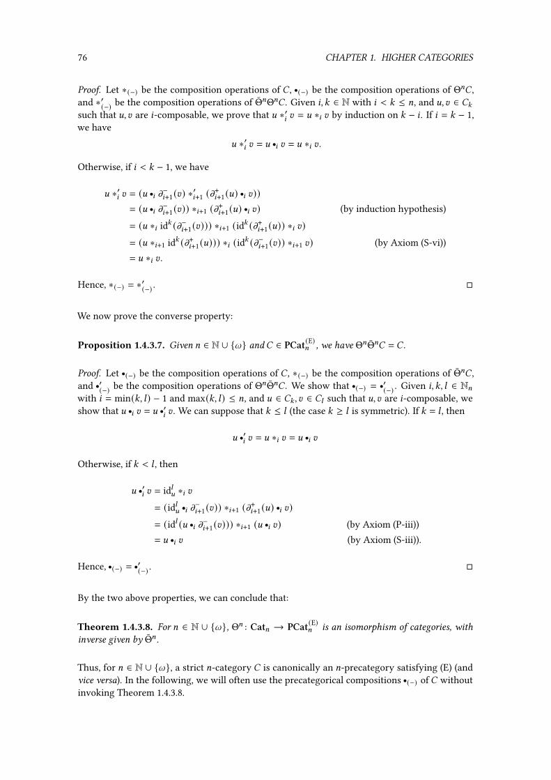
76 CHAPTER 1. HIGHER CATEGORIES

Proof. Let ∗(−) be the composition operations of � , r(−) be the composition operations of Θ=� ,and ∗′(−) be the composition operations of Θ=Θ=� . Given 8, : ∈ N with 8 < : ≤ =, and D, E ∈ �:such that D, E are 8-composable, we prove that D ∗′8 E = D ∗8 E by induction on : − 8 . If 8 = : − 1,we have

D ∗′8 E = D r8 E = D ∗8 E .

Otherwise, if 8 < : − 1, we have

D ∗′8 E = (D r8 m−8+1(E) ∗′8+1 (m+8+1(D) r8 E))

= (D r8 m−8+1(E)) ∗8+1 (m+8+1(D) r8 E) (by induction hypothesis)

= (D ∗8 id: (m−8+1(E))) ∗8+1 (id: (m+8+1(D)) ∗8 E)= (D ∗8+1 id: (m+8+1(D))) ∗8 (id: (m−8+1(E)) ∗8+1 E) (by Axiom (S-vi))= D ∗8 E .

Hence, ∗(−) = ∗′(−) . �

We now prove the converse property:

Proposition 1.4.3.7. Given = ∈ N ∪ {l} and � ∈ PCat(E)= , we have Θ=Θ=� = � .

Proof. Let r(−) be the composition operations of � , ∗(−) be the composition operations of Θ=� ,and r′

(−) be the composition operations of Θ=Θ=� . We show that r(−) = r′(−) . Given 8, :, ; ∈ N=

with 8 = min(:, ;) − 1 and max(:, ;) ≤ =, and D ∈ �: , E ∈ �; such that D, E are 8-composable, weshow that D r

8 E = D r′8 E . We can suppose that : ≤ ; (the case : ≥ ; is symmetric). If : = ; , then

D r′8 E = D ∗8 E = D r

8 E

Otherwise, if : < ; , then

D r′8 E = id;D ∗8 E

= (id;D r8 m−8+1(E)) ∗8+1 (m+8+1(D) r8 E)

= (id; (D r8 m−8+1(E))) ∗8+1 (D r

8 E) (by Axiom (P-iii))= D r

8 E (by Axiom (S-iii)).

Hence, r(−) = r′(−) . �

By the two above properties, we can conclude that:

Theorem 1.4.3.8. For = ∈ N ∪ {l}, Θ= : Cat= → PCat(E)= is an isomorphism of categories, withinverse given by Θ= .

Thus, for = ∈ N ∪ {l}, a strict =-category � is canonically an =-precategory satisfying (E) (andvice versa). In the following, we will often use the precategorical compositions r(−) of � withoutinvoking Theorem 1.4.3.8.

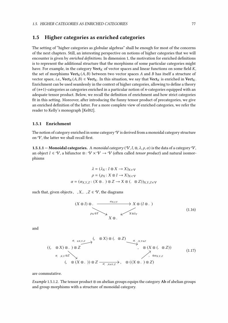
1.5. HIGHER CATEGORIES AS ENRICHED CATEGORIES 77

1.5 Higher categories as enriched categories

The setting of “higher categories as globular algebras” shall be enough for most of the concernsof the next chapters. Still, an interesting perspective on notions of higher categories that we willencounter is given by enriched de�nitions. In dimension 1, the motivation for enriched de�nitionsis to represent the additional structure that the morphisms of some particular categories mighthave. For example, in the category Vect of vector spaces and linear functions on some �eld ,the set of morphisms Vect (�, �) between two vector spaces � and � has itself a structure ofvector space, i.e., Vect (�, �) ∈ Vect . In this situation, we say that Vect is enriched in Vect .Enrichment can be used seamlessly in the context of higher categories, allowing to de�ne a theoryof (=+1)-categories as categories enriched in a particular notion of =-categories equipped with anadequate tensor product. Below, we recall the de�nition of enrichment and how strict categories�t in this setting. Moreover, after introducing the funny tensor product of precategories, we givean enriched de�nition of the latter. For a more complete view of enriched categories, we refer thereader to Kelly’s monograph [Kel82].

1.5.1 Enrichment

The notion of category enriched in some categoryV is derived from a monoidal category structureonV , the latter we shall recall �rst.

1.5.1.1 — Monoidal categories. Amonoidal category (V, � , ⊗, _, d, U) is the data of a categoryV ,an object � ∈ V , a bifunctor ⊗ : V ×V → V (often called tensor product) and natural isomor-phisms

_ = (_- : � ⊗ - → - )- ∈Vd = (d- : - ⊗ � → - )- ∈V

U = (U-,.,/ : (- ⊗ . ) ⊗ / → - ⊗ (. ⊗ / ))-,.,/ ∈V

such that, given objects,,-,., / ∈ V , the diagrams

(- ⊗ � ) ⊗ . - ⊗ (� ⊗ . )

- ⊗ .d- ⊗.

U-,� ,.

- ⊗_.(1.16)

and

(, ⊗ - ) ⊗ (. ⊗ / )

((, ⊗ - ) ⊗ . ) ⊗ /

(, ⊗ (- ⊗ . )) ⊗ / , ⊗ ((- ⊗ . ) ⊗ / )

, ⊗ (- ⊗ (. ⊗ / ))U, ⊗-,.,/ U,,-,.⊗/

U,,-,. ⊗/

U,,-⊗.,/

, ⊗U-,.,/(1.17)

are commutative.

Example 1.5.1.2. The tensor product ⊗ on abelian groups equips the category Ab of abelian groupsand group morphisms with a structure of monoidal category.

78 CHAPTER 1. HIGHER CATEGORIES

Given a category V , if V has all products, then it admits a canonical structure of monoidalcategory (V, 1,×, _, d, U) called the cartesian monoidal structure, where 1 is the terminal objectofV , × is the product operation and _, d and U are the canonical isomorphisms

_ = (_- : 1 × - → - )- ∈Vd = (d- : - × 1→ - )- ∈V

U = (U-,.,/ : (- × . ) × / → - × (. × / ))-,.,/ ∈V

and a similar statement holds ifV has all coproducts.

Example 1.5.1.3. The category Set admits the cartesian monoidal structure (Set, 1,×, U, _, d) de-�ned as above.

1.5.1.4 — Enriched categories. Given a monoidal category (V, � , ⊗, _, d, U), a category enrichedin V is the data of a set �0 and, for all G,~ ∈ �0, an object � (G,~) ∈ V , together with, forall G ∈ �0, a morphism

8G : � → � (G, G) ∈ V

and, for all G,~, I ∈ �0, a morphism

2G,~,I : � (G,~) ⊗ � (~, I) → � (G, I) ∈ V

such that, for allF, G,~, I ∈ �0, the diagrams

� ⊗ � (G,~) � (G, G) ⊗ � (G,~)

� (G,~)_� (G,~)

8G ⊗� (G,~)

2G,G,~(1.18)

and� (G,~) ⊗ � � (G,~) ⊗ � (~,~)

� (G,~)d� (G,~)

� (G,~) ⊗8~

2G,~,~(1.19)

and

(� (F, G) ⊗ � (G,~)) ⊗ � (~, I)

� (F,~) ⊗ � (~, I)

� (F, G) ⊗ (� (G,~) ⊗ � (~, I)) � (F, G) ⊗ � (G, I)

� (F, I)

2F,G,~⊗� (~,I) 2F,~,I

U� (F,G ),� (G,~),� (~,I)

� (F,G) ⊗2G,~,I

2F,G,I

(1.20)

are commutative. Given two categories � and � enriched inV , a morphism between � and � isthe data of a function

�0 : �0 → �0

and, for every G,~ ∈ �0, a morphism

�G,~ : � (G,~) → � (�0(G), �0(~)) ∈ V

1.5. HIGHER CATEGORIES AS ENRICHED CATEGORIES 79

such that the diagrams

�

� (G, G) � (�0(G), �0(G))

8G 8�0 (G )

�G,G

and

� (G,~) ⊗ � (~, I) � (G,~) ⊗ � (~, I)

� (G, I) � (G, I)

2G,~,I

� (G,~) ⊗� (~,I)

2�0 (G ),�0 (~),�0 (I)

� (G,I)

commute for all G,~, I ∈ �0. We write V-Cat for the category of categories enriched in V . Anelementary example of an enriched de�nition is given by the category Cat of small categories,which is equivalent to Set-Cat where Set is equipped with its cartesian monoidal structure. Moregenerally, it is well-known that the category Cat=+1 of strict (=+1)-categories admits an enrichedde�nition based on the cartesian monoidal structure on Cat= :

Theorem 1.5.1.5. Given = ∈ N, considering the cartesian monoidal structure on Cat= , there isan equivalence of categories between Cat=+1 and (Cat=)-Cat. Moreover, considering the cartesianmonoidal structure on Catl , there is an equivalence of categories between Catl and (Catl )-Cat.

Proof. We refer the reader to the existing literature, like [Lei04, Section 1.4]. �

An analogous result can be shown for precategories by considering a monoidal structure di�erentfrom the cartesian one. This is the object of the remainder of this section.

1.5.2 The funny tensor product

Here, we introduce the funny tensor product that we will use as part of a monoidal structure togive an enriched de�nition of precategories. We give a rather direct and concise de�nition, and werefer the reader to the work of Weber [Web09] for a more theoretical de�nition. Let = ∈ N ∪ {l}.Given two =-precategories � and � , the funny tensor product of � and � is the pushout in PCat=

� (0) × � (0) � (0) × �

� × � (0) � � �

i� � (0)

� (0)×i�

r�,�

l�,�

where (−)(0) denotes the functor

(−)PCat↑=,0 (−)

PCat≤0,= : PCat= → PCat=

and i = i0,= is the counit of (−)PCat↑=,0 a (−)

PCat≤0,= . Since i is a natural transformation, the funny tensor

product can be extended to a bifunctor

(−) � (−) : PCat= × PCat= → PCat= .

We show that it equips PCat= with a structure of monoidal category. First, we prove the twoproperties of commutation with colimits below. In the following, we write (PCat=, 1=,×, _, d, U)for the cartesian monoidal structure on PCat= (in particular, 1= is the terminal object of PCat=).

Lemma 1.5.2.1. Given =-precategories � and (�8)8∈� , the canonical morphism∐8∈�(� × �8) → � × (

∐8∈�

�8)

of PCat= is an isomorphism.

80 CHAPTER 1. HIGHER CATEGORIES

Proof. Write � for this morphism. Note that a morphism between =-precategories is an isomor-phism if and only if the underlying morphism of globular sets is an isomorphism. Thus, it issu�cient to show that � induces bijections between the :-cells, i.e., that the images of � underthe functors (−): : PCat= → Set are bijections for : ∈ N= . Products and coproducts are com-puted dimensionwise in PCat= , so that the functors (−): preserve products and coproducts. Sincecoproducts distribute over products in Set, �: is an isomorphism for : ∈ N= , and so is � . �

Lemma 1.5.2.2. Given an =-precategory � , the functor (−) × � (0) : PCat= → PCat= preservescolimits and, dually, the functor � (0) × (−) : PCat= → PCat= preserves colimits.

Proof. Note that, by the de�nition of (−)PCat↑=,0 , we have (10)↑= ' 1= . Since, by Proposition 1.2.3.7,

the functor (−)PCat↑=,0 preserves colimits, we have

� (0) '∐G ∈�0

1= .

Thus, given a diagram � (−) : � → PCat= , by Lemma 1.5.2.1, we have

colim8∈�

�8 × � (0) '∐G ∈�0

colim8∈�

�8 ' colim8∈�(∐G ∈�0

�8) ' colim8∈�(�8 × � (0) ) .

The dual statement is shown similarly. �

We can now de�ne the rest of the monoidal structure for PCat= . Given an =-precategory� , thereare canonical morphisms

_f� : 1= �� → � and d f

� : � � 1= → �

where _f� is de�ned by

1=(0) � (0) 1=(0) �

1= � (0) 1= ��

�

i1= � (0)

1=(0)×i�

r1=,�c2

l1=,�

i� ◦c2

_f�

and d f�

is de�ned similarly. Both are natural in � . Moreover, we have:

Lemma 1.5.2.3. Given � ∈ PCat= , _f� and d f

�are isomorphisms.

Proof. By symmetry, it is su�cient to prove that _f� is an isomorphism. Note that i1= : 1=(0) → 1=

is an isomorphism, so that, by the pushout de�nition of 1= �� , r1=,� is an isomorphism. Moreover,since 1=(0) ' 1= , we have that c2 : 1=(0) × � → � is an isomorphism. Thus, _f

� = r1=,� ◦c−12 is an

isomorphism. �

Furthermore, we introduce the associativity isomorphism with the following lemma:

Lemma 1.5.2.4. Given =-precategories �, �, �, there is an isomorphism

U f�,�,� : (� � �) � � ∼−→ � � (� � �)

natural in �, �, �.

1.5. HIGHER CATEGORIES AS ENRICHED CATEGORIES 81

Proof. The =-precategory (� � �) � � is de�ned by the pushout

(� (0) × � (0) ) × � (0) (� (0) × � (0) ) × �

(� � �) × � (0) (� � �) � �

(� (0)×� (0) )×i�

i��� � (0) r���,�

l���,�

.

Since, by Lemma 1.5.2.2, (−) × � (0) preserves colimits, the following diagram is also a pushout

(� (0) × � (0) ) × � (0) (� (0) × �) × � (0)

(� × � (0) ) × � (0) (� � �) × � (0)

(� (0)×i� )×� (0)

(i� � (0) )� (0) r�,� � (0)

l�,� � (0)

.

So, by expanding the �rst pushout with the second, (� � �) � � can be expressed as the colimit

(� × � (0) ) × � (0)

(� (0) × � (0) ) × � (0) (� (0) × �) × � (0) (� � �) � �

(� (0) × � (0) ) × �

l���,� ◦(l�,� ×� (0) )

(� (0)×i� )×� (0)

(i� � (0) )� (0)

(� (0)×� (0) )×i�

l���,� ◦(r�,� ×� (0) )

r���,�

(1.21)

and � � (� � �) admits a similar diagram. Thus, the isomorphisms

U-,.,/ : (- × . ) × / → - × (. × / ) ∈ PCat=for -,., / ∈ PCat= induce a morphism U f

�,�,�: (� � �) � � → � � (� � �), which is, by the

symmetry of the construction, an isomorphism. It is easily checked to be natural in �, �, �. �

We deduce a monoidal structure for PCat= based on the funny tensor product:

Proposition 1.5.2.5. (�,�, 1=, _f , d f , U f ) is a monoidal category.

Proof. Given �, �,�, � ∈ PCat= , the commutation of the diagram

(� ⊗ 1=) ⊗ � � ⊗ (1= ⊗ �)

� ⊗ �d f�⊗�

U f�,1=,�

�⊗_f�

can be shown using the colimit de�nition of (� � 1=) � � given by (1.21). Moreover, note thatthe object ((� � �) ��) � � admits a de�nition as colimit on a diagram analogous to (1.21) withfour branches. Using this colimit, one can show that the diagram

(� � �) � (� � �)

((� � �) ��) � �

(� � (� ��)) � � � � ((� ��) � �)

� � (� � (� � �))

U f���,�,� U f

�,�,���

U f�,�,�

��

U f�,���,�

��U f�,�,�

commutes. Thus, (�,�, 1=, _f , d f , U f ) is a monoidal category. �

82 CHAPTER 1. HIGHER CATEGORIES

1.5.3 Enriched de�nition of precategories

We now give an enriched de�nition of precategories using the funny tensor product in the formof the following theorem:

Theorem 1.5.3.1. Considering the monoidal structure on PCat= given by the funny tensor pro-duct, there is an equivalence of categories between PCat=+1 and (PCat=)-Cat. Moreover, consideringthe analogous monoidal structure on PCatl , there is an equivalence of categories between PCatland (PCatl )-Cat.

Proof. Given � ∈ PCat=+1, we de�ne an associated object � ∈ (PCat=)-Cat as follows. We put

�0 = �0 and � (G,~) = �↑(G,~)

where �↑(G,~) is the =-precategory such that

(�↑(G,~) )8 = {D ∈ �8+1 | m−0 (D) = G and m+0 (D) = ~}

for 8 ∈ N= and whose composition operation r:,; is the operation r

:+1,;+1 on � for :, ; ∈ N∗= .Given G ∈ �0, we de�ne the identity morphism

8G : 1= → � (G, G)

as the morphism which maps the unique 0-cell ∗ of 1= to id1G ∈ �1. Given G,~, I ∈ �0, we de�ne

the composition morphism

2G,~,I : � (G,~) � � (~, I) → � (G, I) ∈ PCat=

as the unique morphism such that ;G,~,I = 2G,~,I ◦ l� (G,~),� (~,I) is the composite

� (G,~) × � (~, I)(0) '∐

6∈� (~,I)0

� (G,~)[ (−) q06]6∈� (~,I)0−−−−−−−−−−−−−→ � (G, I)

and AG,~,I = 2G,~,I ◦ r� (G,~),� (~,I) is the composite

� (G,~)(0) × � (~, I) '∐

5 ∈� (G,~)0

� (~, I)[5 q0 (−) ]5 ∈� (G,~)0−−−−−−−−−−−−−→ � (G, I).

We verify that the composition morphism is left unital, i.e., given G,~ ∈ �0, the diagram

1= � � (G,~) � (G, G) � � (G,~)

� (G,~)

8G�� (G,~)

_f� (G,~)

2G,G,~

commutes. We compute that

2G,G,~ ◦ (8G � � (G,~)) ◦ l1=,� (G,~) = 2G,G,~ ◦ l� (G,G),� (G,~) ◦(8G × � (G,~)(0) )(by de�nition of �)

= ;G,G,~ ◦ (8G × � (G,~)(0) )= i� (G,~) ◦c2 (by unitality of idG )

= _f� (G,~) ◦ l1=,� (G,~)

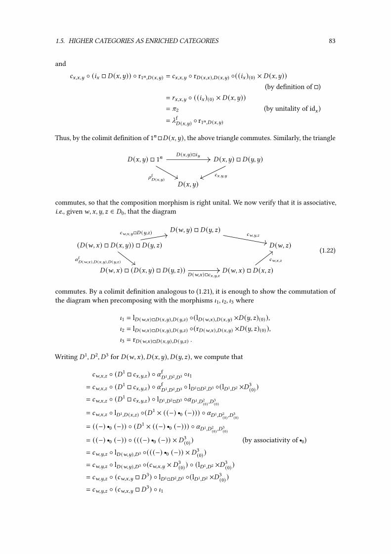
1.5. HIGHER CATEGORIES AS ENRICHED CATEGORIES 83

and

2G,G,~ ◦ (8G � � (G,~)) ◦ r1=,� (G,~) = 2G,G,~ ◦ r� (G,G),� (G,~) ◦((8G )(0) × � (G,~))(by de�nition of �)

= AG,G,~ ◦ ((8G )(0) × � (G,~))= c2 (by unitality of idG )

= _f� (G,~) ◦ r1=,� (G,~)

Thus, by the colimit de�nition of 1=�� (G,~), the above triangle commutes. Similarly, the triangle

� (G,~) � 1= � (G,~) � � (~,~)

� (G,~)

� (G,~)�8~

d f� (G,~)

2G,~,~

commutes, so that the composition morphism is right unital. We now verify that it is associative,i.e., givenF, G,~, I ∈ �0, that the diagram

(� (F, G) � � (G,~)) � � (~, I)

� (F,~) � � (~, I)

� (F, G) � (� (G,~) � � (~, I)) � (F, G) � � (G, I)

� (F, I)

2F,G,~�� (~,I) 2F,~,I

U f� (F,G ),� (G,~),� (~,I)

� (F,G)�2G,~,I

2F,G,I

(1.22)

commutes. By a colimit de�nition analogous to (1.21), it is enough to show the commutation ofthe diagram when precomposing with the morphisms ]1, ]2, ]3 where

]1 = l� (F,G)�� (G,~),� (~,I) ◦(l� (F,G),� (G,~) ×� (~, I)(0) ),]2 = l� (F,G)�� (G,~),� (~,I) ◦(r� (F,G),� (G,~) ×� (~, I)(0) ),]3 = r� (F,G)�� (G,~),� (~,I) .

Writing �1, �2, �3 for � (F, G), � (G,~), � (~, I), we compute that

2F,G,I ◦ (�1 � 2G,~,I) ◦ U f�1,�2,�3 ◦]1

= 2F,G,I ◦ (�1 � 2G,~,I) ◦ U f�1,�2,�3 ◦ l�1��2,�3 ◦(l�1,�2 ×�3

(0) )= 2F,G,I ◦ (�1 � 2G,~,I) ◦ l�1,�2��3 ◦U�1,�2

(0) ,�3(0)

= 2F,G,I ◦ l�1,� (G,I) ◦(�1 × ((−) r0 (−))) ◦ U�1,�2(0) ,�

3(0)

= ((−) r0 (−)) ◦ (�1 × ((−) r0 (−))) ◦ U�1,�2(0) ,�

3(0)

= ((−) r0 (−)) ◦ (((−) r0 (−)) × �3(0) ) (by associativity of r0)

= 2F,~,I ◦ l� (F,~),�3 ◦(((−) r0 (−)) × �3(0) )

= 2F,~,I ◦ l� (F,~),�3 ◦(2F,G,~ × �3(0) ) ◦ (l�1,�2 ×�3

(0) )= 2F,~,I ◦ (2F,G,~ � �3) ◦ l�1��2,�3 ◦(l�1,�2 ×�3

(0) )= 2F,~,I ◦ (2F,G,~ � �3) ◦ ]1

84 CHAPTER 1. HIGHER CATEGORIES

so that the diagram (1.22) commutes when precomposed with ]1 and, similarly, it commutes whenprecomposed with ]2 and ]3. Thus, (1.22) commutes. Hence, � is a category enriched in =-pre-categories. The operation � ↦→ � can easily be extended to morphisms of (=+1)-precategories,giving a functor

� : PCat=+1 → (PCat=)-Cat.

Conversely, given � ∈ (PCat=)-Cat, we de�ne an associated object � ∈ PCat=+1. We put

�0 = �0 and �8+1 =∐G,~∈�0

� (G,~)8

for 8 ∈ N= . Given : ∈ N= , ]G,~ (D) ∈ �:+1 and n ∈ {−, +}, we put

mn:(]G,~ (D)) =

G if : = 0 and n = −,~ if : = 0 and n = +,]G,~ (mn:−1(D)) if : > 0,

so that the operations m−, m+ equips � with a structure of (=+1)-globular set. Given G ∈ �0, weput

id1G = ]G,G (8G (∗))

and, given : ∈ N=−1 and ]G,~ (D) ∈ �:+1, we put

id:+2]G,~ (D) = ]G,~ (id

:+1D ).

Given 8, :1, :2 ∈ N= with 8 = min(:1, :2) − 1, and D = ]G,~ (D) ∈ �:1, E = ]G′,~′ (E) ∈ �:2 that are8-composable, we put

D r8 E =

]G,~ (D r

8 E) if 8 > 0]G,~′ (;G,~,~′ (D, id:1−1

E)) if 8 = 0 and :2 = 1

]G,~′ (AG,~,~′ (id:2−1D

, E)) if 8 = 0 and :1 = 1

where ;G,~,I is the composite

� (G,~) ×� (~, I)(0)l� (G,~),� (~,I)−−−−−−−−−→ � (G,~) �� (~, I)

2G,~,I−−−−→ � (G, I)

and AG,~,I is the composite

� (G,~)(0) ×� (~, I)r� (G,~),� (~,I)−−−−−−−−−−→ � (G,~) �� (~, I)

2G,~,I−−−−→ � (G, I) .

We now have to show that the axioms of (=+1)-precategories are satis�ed. Note that, by thede�nition of � , it is enough to prove the axioms for the id1 and r0 operations. Given G ∈ �0and n ∈ {−, +}, we have

mn0 (id1G ) = mn0 (]G,G (8G (∗))) = G

so that Axiom (P-i) holds. For : ∈ N∗=+1, given D = ]G,~ (D) ∈ �: and E = ]~,I (E) ∈ �1 such that D, Eare 0-composable, if : = 1, then

m−0 (D r0 E) = m−0 (]G,I (;G,~,I (D, E))) = G,

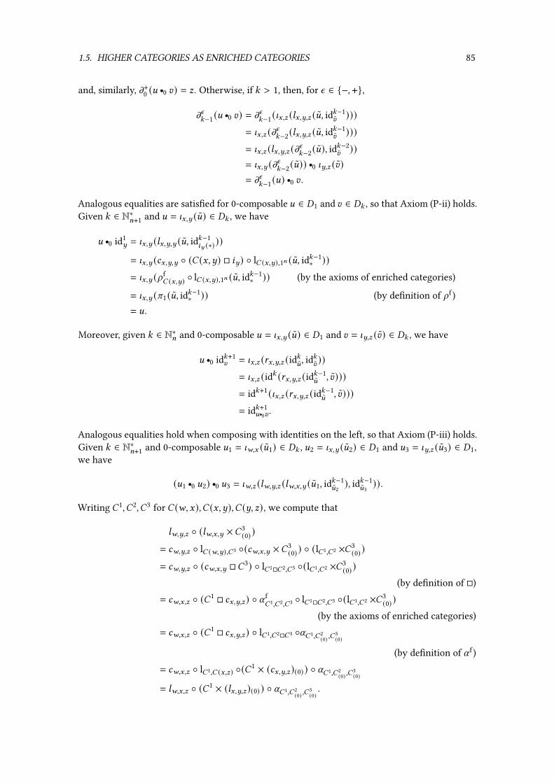
1.5. HIGHER CATEGORIES AS ENRICHED CATEGORIES 85

and, similarly, m+0 (D r0 E) = I. Otherwise, if : > 1, then, for n ∈ {−, +},

mn:−1(D r0 E) = mn:−1(]G,I (;G,~,I (D, id

:−1E )))

= ]G,I (mn:−2(;G,~,I (D, id:−1E )))

= ]G,I (;G,~,I (mn:−2(D), id:−2E ))

= ]G,~ (mn:−2(D)) r0 ]~,I (E)= mn

:−1(D) r0 E .Analogous equalities are satis�ed for 0-composable D ∈ �1 and E ∈ �: , so that Axiom (P-ii) holds.Given : ∈ N∗=+1 and D = ]G,~ (D) ∈ �: , we have

D r0 id1~ = ]G,~ (;G,~,~ (D, id:−1

8~ (∗) ))

= ]G,~ (2G,~,~ ◦ (� (G,~) � 8~) ◦ l� (G,~),1= (D, id:−1∗ ))

= ]G,~ (d f� (G,~) ◦ l� (G,~),1= (D, id:−1

∗ )) (by the axioms of enriched categories)

= ]G,~ (c1(D, id:−1∗ )) (by de�nition of d f )

= D.

Moreover, given : ∈ N∗= and 0-composable D = ]G,~ (D) ∈ �1 and E = ]~,I (E) ∈ �: , we have

D r0 id:+1E = ]G,I (AG,~,I (id:D, id:E ))

= ]G,I (id: (AG,~,I (id:−1D , E)))

= id:+1(]G,I (AG,~,I (id:−1D , E)))

= id:+1D q0E .Analogous equalities hold when composing with identities on the left, so that Axiom (P-iii) holds.Given : ∈ N∗=+1 and 0-composable D1 = ]F,G (D1) ∈ �: , D2 = ]G,~ (D2) ∈ �1 and D3 = ]~,I (D3) ∈ �1,we have

(D1 r0 D2) r0 D3 = ]F,I (;F,~,I (;F,G,~ (D1, id:−1D2), id:−1

D3)).

Writing �1,�2,�3 for � (F, G),� (G,~),� (~, I), we compute that

;F,~,I ◦ (;F,G,~ ×�3(0) )

= 2F,~,I ◦ l� (F,~),�3 ◦(2F,G,~ ×�3(0) ) ◦ (l�1,�2 ×�3

(0) )= 2F,~,I ◦ (2F,G,~ ��3) ◦ l�1��2,�3 ◦(l�1,�2 ×�3

(0) )(by de�nition of �)

= 2F,G,I ◦ (�1 � 2G,~,I) ◦ U f�1,�2,�3 ◦ l�1��2,�3 ◦(l�1,�2 ×�3

(0) )(by the axioms of enriched categories)

= 2F,G,I ◦ (�1 � 2G,~,I) ◦ l�1,�2��3 ◦U�1,�2(0) ,�

3(0)

(by de�nition of U f )= 2F,G,I ◦ l�1,� (G,I) ◦(�1 × (2G,~,I)(0) ) ◦ U�1,�2

(0) ,�3(0)

= ;F,G,I ◦ (�1 × (;G,~,I)(0) ) ◦ U�1,�2(0) ,�

3(0)

.

86 CHAPTER 1. HIGHER CATEGORIES

Thus,

(D1 r0 D2) r0 D3 = ]F,I (;F,G,I (D1, (;G,~,I)(0) (id:−1D2, id:−1

D3)))

= ]F,I (;F,G,I (D1, id:−1(;G,~,I )(0) (D2,D3) ))

= D1 r0 ]G,I ((;G,~,I)(0) (D2, D3))= D1 r0 ]G,I (;G,~,I (D2, D3))= D1 r0 (D2 r0 D3)

and similar equalities can be shown for (D1, D2, D3) ∈ (�1 ×0�: ×0�1) t (�1 ×0�1 ×0�: ), so thatAxiom (P-iv) holds. Finally, for 8, :1, :2, : ∈ N∗=+1 such that 8 = min(:1, :2) − 1, : = max(:1, :2),given D = ]G,~ (D) ∈ �1 and 8-composable E1 = ]~,I (E1) ∈ �:1, E2 = ]~,I (E2) ∈ �:2 , we have

D r0 (E1 r8 E2) = D r0 ]~,I (E1 r

8−1 E2)= ]G,I (AG,~,I (id:−1

D , E1 r8−1 E2))

= ]G,I (AG,~,I (id:1−1D

r8−1 id:2−1

D , E1 r8−1 E2))

= ]G,I (AG,~,I (id:1−1D , E1) r8−1 AG,~,I (id:2−1

D , E2))= ]G,I (AG,~,I (id:1−1

D , E1)) r8 ]G,I (AG,~,I (id:2−1D , E2))

= (D r0 E1) r8 (D r0 E2)

and an analogous equality can be shown for ((D1, D2), E) ∈ ((�:1×8�:2)×0�1), so that Axiom (P-v)holds. Hence, � is an (=+1)-precategory. The construction � ↦→ � extends naturally to enrichedfunctors, giving a functor � : (PCat=)-Cat→ PCat=+1.

Given� ∈ PCat=+1 and� ′ = � ◦ � (�), there is a morphism U� : � → � ′ which is the identitybetween�0 and� ′0 and, for : ∈ N= , maps D ∈ �:+1 to ]G,~ (D) where G = m−0 (D) and ~ = m+0 (D), andone can verify that it is an isomorphism which is natural in � .

Conversely, given� ∈ (PCat=)-Cat and� ′ = � ◦� (�), there is a morphism V : � → � ′ whichis the identity between �0 and � ′0, and, for G,~ ∈ �0, maps D ∈ � (G,~) to ]G,~ (D) ∈ � ′(G,~), andone can verify that it is an isomorphism which is natural in � . Hence, � is an equivalence ofcategories.

A similar proof gives an equivalence of categories between PCatl and (PCatl )-Cat. �

Chapter 2

The word problem on strict categories

Introduction

Given a polygraph of strict categories P, any cell of P∗ can be represented by an expressioninvolving generators of P, and identity id and composition ∗8 operations (c.f. Proposition 1.4.1.16).Typically, several such expressions represent the same cells. For example, given a 1-polygraphwith four composable 1-generators 0, 1, 2, 3 as in

E F G ~ I0 1 2 3

one can verify that the two words

(0 ∗0 (1 ∗0 id1G )) ∗0 (2 ∗0 3) and 0 ∗0 (1 ∗0 (2 ∗0 1)) (2.1)

denote the same 1-cell in the free strict category associated to this polygraph, as a consequence ofthe unitality and the associativity of the composition operation. More generally, the word problemon a polygraph P consists in, given two words on P, deciding whether they evaluate to the samecell of P∗. In order to provide a better understanding and computational treatment of strict highercategories, having an e�cient procedure to solve this problem is important.

As suggested by (2.1), the word problem on strict 1-categories has a quite simple solution.Starting from a word, one obtains a normal form by eliminating the identities and reparenthesizingthe word on the right, and this normal form is essentially a list of composable 1-generators of thepolygraph. One can then decide whether two words represent the same cell by computing andcomparing their normal forms. The word problem in higher dimensions is less simple, since thereis no known orientation of the axioms of strict categories that would allow to rewrite a word bya �nite sequence of moves to a unique normal form.

Still, in [Mak05], Makkai gave a solution to the above word problem. For this purpose, he usedthe equivalent description (recalled in Section 1.4.3) of strict categories as precategories satisfyingan exchange condition to show that words on strict categories admit a canonical form. Moreprecisely, given an =-polygraph P of strict categories, every =-cell D ∈ P∗ can be represented by aword of the form

D1 r=−1 · · · r=−1 D: (2.2)

87

88 CHAPTER 2. THE WORD PROBLEM ON STRICT CATEGORIES

for some : ∈ N∗, where

D8 = ;8,= r=−1 (;8,=−1 r

=−2 · · · r1 (;8,1 r0 68 r0 A8,1) r1 · · · r=−2 A8,=−1) r=−1 A8,=

for 8 ∈ N∗:, with ;8, 9 , A8, 9 ∈ P∗9 and 68 ∈ P= . Then, Makkai showed that a cell D as above admits

a �nite number of canonical forms (2.2) and he introduced a terminating procedure to computethem. This is enough to solve the word problem, since one can then decide whether two wordshave equivalent canonical forms. However, since a cell can admit a lot of canonical forms (2.2),the resulting algorithm is quite ine�cient, which prevents using it to solve too sophisticatedinstances of the word problem.

In his work on the word problem, Makkai introduced several important notions and propertieson polygraphs. Notably, for each polypgraph P, he de�ned a function, that we call Makkai’smeasure, which maps each cell D ∈ P∗ to some element of the free abelian group ZP and whichintuitively counts how many times each generator of P is involved inD. Using this measure, he wasable to prove that his procedure for the word problem terminates. Although Makkai’s measure hasseveral good properties, Makkai remarked that it has the defect of sometimes “double-counting”the generators in the cells. He then raised the question of the existence of another measure onpolygraphs of strict categories which would not display this bad behavior. The existence of sucha measure would be interesting since it could help better characterize the words that representa given cell. It could also help with the study of a special class of polygraphs introduced byMakkai, that he called computopes, and later studied by Henry [Hen17] under the names plexesand polyplexes, following a terminology introduced by Burroni [Bur12]. Intuitively, they arepolygraphs whose generators are “as separated as possible”. Such polygraphs seem to play animportant role in the study of polygraphs. In particular, they can be used to show whether somesubcategories of polygraphs are presheaf categories, as witnessed by the works of Makkai andHenry.

Outline. This chapter is mainly concerned with giving an e�cient and implementable solutionto the word problem on polygraphs of strict categories. It is organized as follows. First, werecall the de�nition of Makkai’s measure and use it to prove several basic properties of freestrict categories on polygraphs (Section 2.1). Next, we introduce a description of the cells of freecategories which is better suited for solving the word problem than the canonical forms of Makkai(Section 2.2), and, after introducing some computability formalism on higher categories, we showthat this description is amenable to computations (Section 2.3). We then deduce a procedure tosolve the word problem on �nite polygraphs and show how it can be used to solve the wordproblem on general polygraphs (Section 2.4), and we moreover provide an implementation of itin OCaml (Section 2.4.4). Our procedure strongly resembles the one given by Makkai but witha stronger emphasis put on e�ciency, so that the resulting algorithm can be used to solve non-trivial instances of the word problem. Finally, we answer the question raised by Makkai and showthat there is no such thing as a measure on polygraphs of strict categories which does not doublecounts generators (Section 2.5).

2.1 Measures on polygraphs

Given = ∈ N, considering the number of axioms of strict =-categories, it is actually not trivialto decide simple properties of the free =-category generated on some polygraph P. For example,given two di�erent =-generators U and V of P, it is not immediate that they induce di�erent cellsin the =-category P∗. Indeed, it could be the case that a sequence of instances of the axioms ofl-categories leads to an identi�cation of U and V . Another example is that it is not immediate

2.1. MEASURES ON POLYGRAPHS 89

that generators of P induce undecomposable cells in P∗. Even though it is “well-known” thatthese two properties hold in free =-categories, the precise argument can be hard to write down.In order to solve quickly this kind of questions, Makkai [Mak05] introduced a function P∗ → ZPthat assesses the complexity of the cells of P∗; more precisely, this function gives some accounton how many times the generators of P are used to de�ne a speci�c cell of P∗, so that we call thisfunction a “measure”. It admits a simple inductive de�nition (c.f. Proposition 2.1.2.9) but the proofof its correctness given by Makkai is quite involved. Later, Henry [Hen18] introduced anothermeasure on polygraphs which has a more natural de�nition, and from which Makkai’s measurecan be derived. The latter still display better properties, notably positivity, which make it moreconvenient to work with in general than Henry’s measure.

In this section, we recall the de�nition of Makkai’s measure, by deriving it from Henry’smeasure, and use it to show several elementary properties of free categories. For this purpose,we follow [Hen18] and introduce the notions of =-globular groups and of =-groups, together withthe equivalence between the two (Section 2.1.1). Henry’s measure is then de�ned as the universalmorphism of the free =-globular group on a polygraph, and one derives Makkai’s measure bya change of base (Section 2.1.2). Finally, following [Mak05], we use Makkai’s measure to proveseveral elementary properties of free =-categories (Section 2.1.3) that will need in the followingsections.

2.1.1 n-globular groups and n-groups

Here, we de�ne =-globular groups and =-groups and prove an equivalence between the two.Moreover, we show that there is a free =-globular group on an =-category. These notions willbe used to de�ne Henry’s measure as the universal morphism of the free =-group on the strict=-category generated by a polygraph. All the content here can be found in [Hen18].

2.1.1.1 — De�nitions. Let = ∈ N ∪ {l}. An =-globular group is the data of an abelian group �together with group morphisms

m−8 , m+8 : � → �

for 8 ∈ N=−1 satisfying, for :, ; ∈ N=−1 and X, n ∈ {−, +},

mX:◦ mn

;=

{mX:

if : < ; ,mn;

if : ≥ ; ,

and, when = = l , the following condition is moreover satis�ed:

for every D ∈ � , there exists 8 ∈ N such that m−8 (D) = D. (2.3)

Given =-globular groups � and � ′, an =-globular groups morphism between � and � ′ is a groupmorphism 5 : � → � ′ such that mn8 ◦ 5 = 5 ◦ mn8 for 8 ∈ N=−1 and n ∈ {−, +}. We write gGrp= forthe category of =-globular groups.

An =-group is an =-category object in the category of abelian groups Ab, i.e., it is the data ofa sequence of abelian groups (�: ):∈N= together with

– group morphisms m−8 , m+8 : �8+1 → �8 for 8 ∈ N=−1,

– group morphisms id:+1 : �: → �:+1 for : ∈ N=−1,

– group morphisms ∗8,: : �: ×8 �: → �: for 8, : ∈ N= with 8 < : ,

90 CHAPTER 2. THE WORD PROBLEM ON STRICT CATEGORIES

satisfying the axioms of strict =-categories (c.f. Paragraph 1.4.1.1). Given two =-groups (�: ):∈N=and (�: ):∈N= , an =-group morphism from (�: ): to (�: ): is an =-functor � : (�: ): → (�: ): suchthat �: is a group morphism for : ∈ N= . We write Grp= for the category of =-groups. The=-groups have the property that composition operations can be derived from the rest:

Proposition 2.1.1.2. Given an =-group (�: ):∈N= , 8, 9 ∈ N= with 8 < 9 and 8-composable D, E ∈ � 9 ,we have D ∗8 E = D + E − id9 (m+8 (D)).

Proof. Indeed, in the abelian group � 9 ×8 � 9 , we have

(D, E) = (D, id9 (m+8 (D))) + (id9 (m−8 (E)), E) − (id9 (m−8 (E)), id9 (m+8 (D)))= (D, id9 (m+8 (D))) + (id9 (m−8 (E)), E) − (id9 (m+8 (E)), id9 (m+8 (D)))

so that D ∗8 E = D + E − id9D . �

2.1.1.3 — Equivalence. Let = ∈ N ∪ {l}. Given an =-group (�: ):∈N= , we de�ne an =-globulargroup� such that� = �= and mn8 = id=8 ◦ mn8 for 8 ∈ N=−1 and n ∈ {−, +} by taking the conventionthat, when = = l , the abelian group �l is de�ned as a colimit cocone (idl

:: �: → �l ):∈N on the

diagram

�0 �1 · · · �: �:+1 · · ·id1

0 id21 id:

:−1 id:+1:

id:+2:+1

and that the function mn8 : �l → �8 for 8 ∈ N and n ∈ {−, +} are de�ned as the unique functionssuch that mn8 ◦ idl9 = mn8 for 9 ∈ N with 8 ≤ 9 . Indeed, given :, ; ∈ N=−1 and X, n ∈ {−, +}, if : < ; ,then

mX:◦ mn

;= id=

:◦ mX

:◦ id=

;◦ mn

;

= id=:◦ mX

:◦ mn

;

= id=:◦ mX

:

= mX:

and, if otherwise : ≥ ; , then

mX:◦ mn

;= id=

:◦ mX

:◦ id=

;◦ mn

;

= id=:◦ id:

;◦ mn

;

= id=;◦ mn

;

= mn;

so that � is an =-globular group. The construction (�: ): ↦→ � extends to a functor

H : Grp= → gGrp= .

Conversely, given an =-globular group � , we de�ne an =-group (�: ):∈N= as follows. For : ∈ N= ,we de�ne the abelian groups �: as the subgroups of � such that

�: � �m−:

1�(2.4)

is an equalizer, taking the convention that m−= = 1� . When : ≤ = − 2, for D ∈ �: , we have

m−:+1(D) = m

−:+1 ◦ m

−:(D) = m−

:(D) = D

2.1. MEASURES ON POLYGRAPHS 91

so that, by the universal property of the equalizer, there is a morphism id:+1:

: �: → �:+1, andwe write id==−1 : �=−1 → �= for the embedding of �=−1 in � = �= . Moreover, for all n ∈ {−, +}and : ∈ N=−1, we de�ne mn

:: �:+1 → �: as the unique factorization map in the diagram

�:+1 � �

�: � �

mn:

m−:+1

1�mn:

mn:

m−:

1�

.

Finally, for 8, : ∈ N= with 8 < : , we de�ne a composition operation ∗8,: : �: ×8�: → �: by putting

D ∗8,: E = D + E − id:m+8(D)

for (D, E) ∈ �: ×8 �: , which makes ∗8,: a group morphism. We verify that:

Proposition 2.1.1.4. The operations id8+18 , m−8 , m+8 for 8 ∈ N=−1, and ∗8,: for 8, : ∈ N= with 8 < : ,

equip (�: ):∈N= with a structure of an =-group.

Proof. For 8 ∈ N=−2 and n ∈ {−, +}, we have mn8 ◦ m−8+1 = mn8 ◦ m+8+1 from the fact that

mn8 ◦ m−8+1 = mn8 = mn8 ◦ m+8+1

so the operations m−8 , m+8 for 8 ∈ N=−1 equip (�8)8∈N= with a structure of globular set in Ab. We

now show that the axioms of =-category are satis�ed with the other operations.

Proof of Axiom (S-i): Let : ∈ N=−1, n ∈ {−, +} and D ∈ �: . We have

mn:(id:+1D ) = mn: (D) (by de�nition of id:+1

:and mn

:)

= D (by the equalizer de�nition of �: ).

Thus, Axiom (S-i) holds.

Proof of Axiom (S-ii): Let 8, : ∈ N= with 8 < : , (D, E) ∈ �: ×8 �: and n ∈ {−, +}. Then,

mn:−1(D ∗8 E) = m

n:−1(D + E − id:

m+8(D) )

= mn:−1(D) + m

n:−1(E) − m

n:−1(id

:m+8(D) )

so that, if 8 < : − 1, then

mn:−1(D ∗8 E) = m

n:−1(D) + m

n:−1(E) − id:−1

m+8(D) (by Axiom (S-i))

= mn:−1(D) ∗8 (m

n:−1(E))

and otherwise if 8 = : − 1, then

mn:−1(D ∗8 E) =

{m−:−1(D) + m

−:−1(E) − m

+:−1(D) = m

−:−1(D) if n = − ,

m+:−1(D) + m

+:−1(E) − m

+:−1(D) = m

+:−1(E) if n = + .

Thus, Axiom (S-ii) holds.

Proof of Axiom (S-iii): Let 8, : ∈ N= with 8 < : and D ∈ �: . We have

id:m−8(D) ∗8 D = id:

m−8(D) + D − id:

m−8(D) (by Axiom (S-i))

= D

92 CHAPTER 2. THE WORD PROBLEM ON STRICT CATEGORIES

and, similarly, D ∗8 id:m+8(D) = D. Thus, Axiom (S-iii) holds.

Proof of Axiom (S-iv): Let 8, : ∈ N= with 8 < : and 8-composable D1, D2, D3 ∈ �: . Then,

(D1 ∗8 D2) ∗8 D3 = (D1 ∗8 D2) + D3 − id:8 (m+8 (D1 ∗8 D2))= (D1 ∗8 D2) + D3 − id:8 (m+8 (D2)) (by Axiom (S-ii))

= D1 + D2 + D3 − id:8 (m+8 (D1)) − id:8 (m+8 (D2)) (by Axiom (S-ii))

and, similarly,

D1 ∗8 (D2 ∗8 D3) = D1 + D2 + D3 − id:8 (m+8 (D1)) − id:8 (m+8 (D2))

so that (D1 ∗8 D2) ∗8 D3 = D1 ∗8 (D2 ∗8 D3). Thus, Axiom (S-iv) holds.

Proof of Axiom (S-v): Let 8, 9, : ∈ N= with 8 < 9 < : and (D1, D2) ∈ � 9 ×8 � 9 . Then,

id:D1 ∗8 id:D2 = id:D1 + id:D2 − id:m+8(id:9 (D1))

= id:D1 + id:D2 − id:m+8(D1) (by Axiom (S-i))

= D1 + D2 − id9m+8(D1) (since id:9 is the embedding � 9 ⊆ �: )

= D1 ∗8 D2

= id:D1∗8D2 (since id:9 is the embedding � 9 ⊆ �: ).

Thus, Axiom (S-v) holds.

Proof of Axiom (S-vi): Let 8, 9, : ∈ N= with 8 < 9 < : , and D1, E1, D2, E2 ∈ �: such that D; , E; are9-composable for ; ∈ {1, 2} and D1, D2 are 8-composable. We have

(D1 ∗9 E1) ∗8 (D2 ∗9 E2) = (D1 ∗9 E1) + (D2 ∗9 E2) − id:8 (m+8 (D1)) (by Axiom (S-ii))

= D1 + E1 − id:9 (m+9 (D1)) + D2 + E2 − id:9 (m+9 (D2)) − id:8 (m+8 (D1))= D1 + D2 − id:8 (m+8 (D1)) + E1 + E2 − id:8 (m+8 (E1))− id:9 (m+9 (D1)) − id:9 (m+9 (D2)) + id:8 (m+8 (D1))

= D1 ∗8 D2 + E1 ∗8 E2 − id:9 (m+9 (D1)) ∗8 id:9 (m+9 (D2))= (D1 ∗8 D2) + (E1 ∗8 E2) − id:9 (m+9 (D1 ∗8 D2)) (by Axiom (S-v))= (D1 ∗8 D2) ∗9 (E1 ∗8 E2).

Thus, Axiom (S-vi) is satis�ed. Hence, (�: ):∈N is equipped with a structure of an =-category. �

The construction � ↦→ (�: ):∈N= extends to a functor

K : gGrp= → Grp=

The two constructions witness that =-globular groups are equivalent to =-groups:

Proposition 2.1.1.5. The functorsH andK exhibit an equivalence of categories between =-groupsand =-globular groups.

2.1. MEASURES ON POLYGRAPHS 93

Proof. Let � = (�: ):∈N= be an =-group and � = H� . Given : ∈ N= , since � = �= , �: can berecovered up to isomorphism as the equalizer

�: � �id=:

m−:

1�

and, when : < =, since

m−:+1 ◦ id=

:= m−

:+1 ◦ m−:◦ id=

:= m−

:◦ id=

:= id=

:

the morphism id:+1:

: �: → �:+1 is the unique morphism such that id=:+1 ◦ id:+1

:= id=

:. Now,

given 8 ∈ N=−1 and n ∈ {−, +}, mn8 : �8+1 → �8 is the unique morphism which makes the left squareof

�8+1 � �

�8 � �

id=8+1

mn8

m−8+1

1�mn8

mn8

id=8

m−8

1�

commute. Finally, by Proposition 2.1.1.2, the composition operations ∗8,: for 8, : ∈ N= with 8 < :can be recovered from mn8 and id:8 . Thus, we have an isomorphism � ' KH� which is naturalin � .

Conversely, given an =-globular group� and� = K� , we have� = �= (when = = l , we havethat � ' �l by the condition (2.3)). Moreover, for 8 ∈ N=−1 and n ∈ {−, +}, we have mn8 = id=8 ◦ mn8Thus, we have an isomorphism � ' HK� which is natural in � . �

2.1.1.6 — Free n-groups. Given a set ( , we write Z(() for the free abelian group on ( . Let � bean =-category � . We write |� | for the set

|� | =⊔8∈N=

�8 .

We de�ne the linearization of � as the abelian group Z� which is the quotient of Z( |� |) by thesubgroup generated by

(i) D − id:+1:(D) for : ∈ N=−1 and D ∈ �: ,

(ii) D ∗8 E − D − E + id: (m+8 (D)) for 8, : ∈ N= with 8 < : and 8-composable D, E ∈ �: .

Moreover, we writeÈ−É : Z( |� |) → Z�

for the canonical projection.

Proposition 2.1.1.7. There exist group morphisms mn8 : Z� → Z� for 8 ∈ N=−1 and n ∈ {−, +} thatare unique such that, for all : ∈ N= and D ∈ �: ,

mn8 (ÈDÉ) ={Èmn8 (D)É if 8 < : ,ÈDÉ if 8 ≥ : ,

and these morphisms equip Z� with a structure of =-globular group.

94 CHAPTER 2. THE WORD PROBLEM ON STRICT CATEGORIES

Proof. For 8 ∈ N=−1 and n ∈ {−, +}, by the universal property of the free abelian group, there is aunique group morphism mn8 between Z|� | and Z� which satis�es that, for all : ∈ N= and D ∈ �: ,

mn8 (D) ={Èmn8 (D)É if 8 < : ,ÈDÉ if 8 ≥ : .

We show that mn8 can be factored through Z� by verifying the quotient equations. Given : ∈ N=−1and D ∈ �: , we have

mn8 (D − id:+1D ) = mn8 (D) − mn8 (id:+1D )

=

{Èmn8 (D)É − Èmn8 (id

:+1D )É = Èmn8 (D)É − Èmn8 (D)É if 8 ≤ : ,

ÈDÉ − Èid:+1D É if 8 > : ,

= 0

and, given 9, : ∈ N= with 9 < : and 9-composable D, E ∈ �: , we have

mn8 (D ∗9 E − D − E + id:9 (m+9 (D))) = mn8 (D ∗9 E) − mn8 (D) − mn8 (E) + mn8 (id:9 (m+9 (D))).

If 8 < 9 , then

mn8 (D ∗9 E − D − E + id:9 (m+9 (D))) = Èmn8 (D)É − Èmn8 (D)É − Èmn8 (D)É + Èm−8 (D)É = 0

else, if 8 = 9 and n = −, then, since m+8 (D) = m−8 (E),

mn8 (D ∗9 E − D − E + id:9 (m+9 (D))) = Èm−8 (D)É − Èm−8 (D)É − Èm−8 (E)É + Èm+8 (D)É = 0

and similarly when n = +. Else, if 9 < 8 < : , then

mn8 (D ∗9 E − D − E + id:9 (m+9 (D))) = Èmn8 (D) ∗9 mn8 (D)É − Èmn8 (D)É − Èmn8 (E)É + Èid89 (m+9 (D))É = 0

and otherwise, if : < 8 , then

mn8 (D ∗9 E − D − E + id:9 (m+9 (D))) = ÈD ∗9 EÉ − ÈDÉ − ÈEÉ + Èid:9 (m+9 (D))É = 0

so mn8 factors through Z� , which gives mn8 : Z� → Z� . Moreover, for X, n ∈ {−, +} and 8, 9 ∈ N= ,given : ∈ N= and D ∈ �: , if 8 < 9 , then

mX8 ◦ mn9 (ÈDÉ) ={mX8(ÈDÉ) if 8 < : ,ÈDÉ = mX

8(ÈDÉ) if 8 ≥ : ,

and else, if 8 ≥ 9 , then

mX8 ◦ mn9 (ÈDÉ) ={mn9 (ÈDÉ) if 9 < : ,ÈDÉ = mn9 (ÈDÉ) if : ≤ 9 ,

so that, since ÈDÉ generates Z� for D ∈ |� |,

mX8 ◦ mn9 ={mX8

if 8 < 9 ,mn9 if 8 ≥ 9 .

Moreover, when = = l , we easily see from the de�nition of Z� and the functions m−8 , m+8 that

the condition (2.3) is satis�ed. Thus, the morphisms (m−8 )8∈N=−1 and (m+8 )8∈N=−1 equip Z� with astructure of =-globular group. �

2.1. MEASURES ON POLYGRAPHS 95

Using the equivalence of Proposition 2.1.1.5, we write ((Z�): ):∈N= for the =-group associated tothe =-globular group Z� . Given : ∈ N= , let Z(�: ) be the quotient of the free abelian group Z(�: )by the subgroup generated by the terms D ∗8 E − D − E + id:8 (m+8 (D)) for 8 ∈ N:−1 and 8-compo-sable D, E ∈ �: and let

È−É: : Z(�: ) → Z(�: )

be the associated projection morphism. The restriction of È−É : Z( |� |) → Z� to Z(�: ) induces amorphism

q: : Z(�: ) → Z�

which satis�es m−:◦ q: = q: since, for all D ∈ �: ,

m−:◦ q: (ÈDÉ: ) = m−: (ÈDÉ) = ÈDÉ = q: (ÈDÉ: ).

Thus, by the equalizer de�nition of (Z�): (c.f. (2.4)), this induces a morphismk: : Z(�: ) → (Z�): .

Proposition 2.1.1.8. For all : ∈ N= ,k: is an isomorphism.

Proof. We build a retraction q: : Z� → Z(�: ) to q: as follows. We �rst de�ne

q: : Z( |� |) → Z(�: )

as the unique morphism such that, for ; ∈ N= and D ∈ �; ,

q: (D) =

Èid:

;(D)É: if ; < : ,

ÈDÉ: if ; = : ,Èm−:(D)É: if ; > : .

We compute that, for ; ∈ N=−1 and D ∈ �; ,

q: (D − id;+1D ) =

id:D − id:D if ; < : ,D − D if ; = : ,m−:(D) − m−

:(D) if ; > : ,

= 0

and, for 8, ; ∈ N= with 8 < ; and 8-composable D, E ∈ �; , if ; < : , then

q: (D ∗8 E − D − E + id;8 (m+8 (D))) = Èid:D ∗8 id:EÉ: − Èid:DÉ: − Èid:EÉ: + Èid:m+8(id:D )É: = 0

else if 8 < : ≤ ; , then

q: (D ∗8 E − D − E + id;8 (m+8 (D))) = Èm−: (D) ∗8 m−:(E)É − Èm−

:(D)É − Èm−

:(E)É + Èid:8 (m+8 (D))É = 0

and otherwise, if : ≤ 8 , then

q: (D ∗8 E − D − E + id;8 (m+8 (D))) = Èm−: (D)É − Èm−:(D)É − Èm−

:(E)É + Èm−

:(E)É = 0.

Thus, q: induces a morphism q: : Z� → Z(�: ) and, for D ∈ �: , we have

q: ◦ q: (ÈDÉ: ) = q: (ÈDÉ) = ÈDÉ:

96 CHAPTER 2. THE WORD PROBLEM ON STRICT CATEGORIES

so that q: ◦ q: = 1Z(�: ) . Moreover, for ; ∈ N=−1 and D ∈ |� |, we compute that

q: ◦ q: ◦ m−: (ÈDÉ) ={Èm−:(D)É = m−

:(ÈDÉ) if : < ; ,

Èid:;(D)É = ÈDÉ = m−

:(ÈDÉ) if : ≥ ; ,

so that q: ◦ q: ◦ m−: = m−:

. We then de�ne k: as the composite

(Z�): Z� Z(�: )]: q:

where ]: : (Z�): → Z� is the embedding of the equalizer (2.4). We have

k: ◦k: = q: ◦ ]: ◦k:= q: ◦ q:= 1Z(�: ) .

Conversely, we have

]: ◦k: ◦ k: = q: ◦ q: ◦ ]:= q: ◦ q: ◦ m−: ◦ ]: (by the de�nition of ]: )= m−

:◦ ]: (since q: ◦ q: ◦ m−: = m−

:)

= ]:

so that, since ]: is a monomorphism, we havek: ◦ k: = 1(Z�): . Thus,k: : Z(�: ) → (Z�): is anisomorphism. �

The above property allows us to implicitly identify (Z�): and Z(�: ), and denote both by Z�: .We now write

(X� ): : �: → Z�:for the function which maps D ∈ �: to ÈDÉ: ∈ Z�: . We have:

Proposition 2.1.1.9. The functions (X� ): for : ∈ N= de�ne a functor X� : � → Z� of =-categories,which exhibit Z� as the free =-group on � .

Proof. We verify that X� is a functor. Given : ∈ N=−1, n ∈ {−, +} and D ∈ �:+1, we have

X� (m−: (D)) = Èm−:(D)É = m−

:(ÈDÉ) = m−

:(X� (D))

so X� is a morphism of =-globular set. Moreover, given : ∈ N=−1 and D ∈ �: , we have

X� (id:+1:(D)) = Èid:+1

:(D)É = ÈDÉ = id:+1

:(ÈDÉ) = id:+1

:(X� (D))

and, given 8, : ∈ N= with 8 < : and 8-composable D, E ∈ �: ,

X� (D ∗8 E) = ÈD ∗8 EÉ = ÈDÉ + ÈEÉ − Èid:8 (m+8 (D))É = ÈDÉ ∗8 ÈEÉ = X� (D) ∗8 X� (E).Hence, X� de�nes an =-functor X� : � → Z� .Now let � : � → � be an =-functor where� is an =-category equipped with a structure of =-group.For all : ∈ N=−1 and D ∈ �: , we have

� (id:+1D ) = id:+1� (D)

and, for 8, : ∈ N= with 8 < : and 8-composable D, E ∈ �: , we have

� (D ∗8 E) = � (D) ∗8 � (E) = � (D) + � (E) − id: (m+8 (� (D))).Thus � factor through X� , which gives a morphism of =-group � ′ : Z� → � satisfying � ′ ◦X� = �

and such an � ′ is uniquely de�ned by � ′ ◦ X� (6) = � (6) for 6 ∈ � . Thus, Z� is the free =-groupon � . �

2.1. MEASURES ON POLYGRAPHS 97

2.1.2 Measures on polygraphs

In this section, we introduce Henry’s and Makkai’s measures on polygraphs. Henry’s measure isde�ned as the specialization of the linearization function seen in Paragraph 2.1.1.6 on polygraphs,and Makkai’s measure will be derived from Henry’s with a change of basis.

2.1.2.1 — Henry’s measure. Let = ∈ N ∪ {l}. Given an =-polygraph P, we write |P| for

|P| =⊔:∈N=

P: .

We have the following other characterization of the free =-group in the case of a free =-categoryon an =-polygraph:

Proposition 2.1.2.2. Let P be an =-polygraph. There exist functions

mn8 : Z( |P |) → Z( |P |)

for n ∈ {−, +} and 8 ∈ N=−1 that equip Z( |P |) with a structure of =-globular group (or, equivalently,=-group) such that the embedding |P| ↩→ Z( |P |) induces an =-functor

XP : P∗ → Z( |P |)

which exhibits Z( |P |) as the free =-group on P∗.

Proof. We show this property by induction on=. When= = 0, the property holds sinceZP∗ = Z( |P |)for all 0-polygraph P. So suppose that the property holds for some = ∈ N. We show that it holdsfor = +1. Let P = (Q, P=+1) be an (=+1)-polygraph. By induction hypothesis, there are morphisms

mn8 : Z( |Q |) → Z( |Q |)

for n ∈ {−, +} and 8 ∈ N= that equip Z( |Q |) with a structure of =-globular group, and such that theinclusion Q ↩→ Z( |Q |) induces an =-functor XQ : Q∗ → Z( |Q |) (where Z( |Q |) is equipped with thestructure of =-group coming from Proposition 2.1.1.5). For n ∈ {−, +}, let mn= : Z( |Q |) → Z( |Q |) bethe identity 1Z( |Q |) . For 8 ∈ N= and n ∈ {−, +}, we extend the group morphisms mn8 : Z( |Q |) → Z( |Q |)to morphisms mn8 : Z( |P |) → Z( |P |) by putting

mn8 (6) = XQ (mn8 (6))

for 6 ∈ P=+1. We check that, given 8, 9 ∈ N= and X, n ∈ {−, +} and 6 ∈ P=+1, if 8 < 9 , then

mX8 ◦ mn9 (6) = mX8 (XQ (mn9 (6)))= XQ (mX8 (mn9 (6)))= XQ (mX8 (6))= mX8 (6)

and otherwise, if 8 ≥ 9 , then

mX8 ◦ mn9 (6) = mX8 (XQ (mn9 (6)))= XQ (mn9 (6)) (since XQ (mn9 (6)) ∈ (Z( |P |) )9 )= mn9 (6).

98 CHAPTER 2. THE WORD PROBLEM ON STRICT CATEGORIES

Thus, the functions mn8 : Z( |P |) → Z( |P |) for 8 ∈ N= and n ∈ {−, +} equip Z( |P |) with a structure of(=+1)-globular group, from which we derive a structure of (=+1)-group using Proposition 2.1.1.5.Since, for 6 ∈ P=+1 and n ∈ {−, +}, we have

mn= (XQ (6)) = mn= (XQ (6)) = XQ (mn= (6))

the =-functor XQ : Q∗ → Z( |Q |) can be extended to an (=+1)-functor XP : P∗ → Z( |P |) suchthat XP(6) = 6 for every 6 ∈ P.

We now prove that Z( |P |) is the free (=+1)-group on P∗. Let � : P∗ → � be an (=+1)-functorwhere � is an =-category equipped with a structure of (=+1)-group. By induction hypothesis,there exists a unique =-functor � ′ : Z( |Q |) → �≤= such that �≤= = � ′ ◦ XQ . Seeing � ′ as amorphism of gGrp= , we extend � ′ to a group morphism � : Z( |P |) → � by putting � (6) = � (6)for 6 ∈ P=+1. For n ∈ {−, +} and 6 ∈ P=+1, we compute

� (mn= (6)) = � ′(XQ (mn= (6)))= � (mn= (6))= mn= (� (6))= mn= (� (6))

so that � ◦ mn= = mn= ◦ � . Thus, � is an (=+1)-globular group morphism, or equivalently, an(=+1)-group morphism. Moreover, since

� ◦ XP(6) = � (6) = � (6)

for all 6 ∈ P, we have� ◦ XP = � and� is uniquely determined by this condition. Hence, Z( |P |) isthe free (=+1)-group on P∗.

Finally, if = = l , then, since Z( |P |) ' ⋃:∈N Z

( |P≤: |) , we derive a structure of l-globulargroup on Z( |P |) from the structures of :-globular groups of Z( |P≤: |) for : ∈ N, for which we havecanonical isomorphisms

(Z( |P |) )≤: ' Z( |P≤: |)

as :-groups. By Proposition 1.2.3.12, the :-functors XP≤: induce an l-functor

XP : P∗ → Z( |P |) .

Moreover, we can verify that, for : ∈ N, the adjunctions (−)Cat↑l,: a (−)

Cat≤:,l : Catl → Cat: restrict

to adjunctions Grpl → Grp: , so that, given � ∈ Grpl ,

Catl (P∗,�) ' lim:∈N

Cat: (P∗≤: ,�≤: )

' lim:∈N

Grp: (Z( |P≤: |) ,�≤: )

' lim:∈N

Grp: ((Z( |P |) )≤: ,�≤: )

' Grpl (Z( |P |) ,�)

which exhibits Z( |P |) as the free l-group on P∗, with XP as universal morphism. �

Thus, given an =-polygraph P, by Proposition 2.1.2.2, ZP∗ is the free abelian group on |P|, orequivalently, the free/ -module on |P|, so that we prefer to write ZP for ZP∗. We equip ZP with thebasis (XP(6))6∈P and, in fact, we simply write 6 for XP(6). Moreover, given a morphism � : P→ Q

2.1. MEASURES ON POLYGRAPHS 99

in Pol= , we write Z� : ZP→ ZQ for the=-functor such that Z� (6) = � (6) for6 ∈ P. GivenD ∈ ZP,we write (D6)6∈ |P | ∈ Z |P | for the family such that

D =∑6∈ |P |

D66 .

Moreover, given D, E ∈ ZP, we write D ≤ E when D6 ≤ E6 for every 6 ∈ P, and we say that D ispositive when 0 ≤ D.

We call the function XP : |P∗ | → ZP the Henry’s measure on the polygraph P. By the de�nitionof XP in Proposition 2.1.2.2 and Proposition 2.1.1.2, XP admits the following inductive de�nition:

– XP(6) = 6 for 6 ∈ P,

– XP(id:+1D ) = XP(D) for : ∈ N=−1 and D ∈ P∗:,

– XP(D ∗8 E) = XP(D) + XP(E) − XP(m+8 (D)) for 8, : ∈ N= with 8 < : and 8-composable D, E ∈ P∗:.

Moreover, Henry’s measure is natural in P:

Proposition 2.1.2.3. Given a morphism � : P→ Q in Pol= , we have

Z� ◦ XP = XQ ◦ |� ∗ |.

Proof. By functoriality, it is enough to check this equality for 6 ∈ P:

Z� ◦ XP(6) = Z� (6) = � (6) = XQ (� (6)). �

However, Henry’s measure is not positive in general, i.e., we do not have XP(D) ≥ 0 for all D ∈ P∗.Example 2.1.2.4. Consider the 2-polygraph P with

P0 = {G,~, I}, P1 = {51, 52, 53 : G → ~, 6 : ~ → I}, and P2 = {U1 : 51 ⇒ 52, U2 : 52 ⇒ 53}

as in

G ~ I

51

52

53

6⇓ U1

⇓ U2

.

Given the 2-cell D = (U1 ∗1 U2) ∗0 id26, we compute XP(D):

XP(D) = XP(U1 ∗1 U2) + XP(id26) − XP(m+0 (U1 ∗1 U2))

= XP(U1) + XP(U2) − XP(m+1 (U1)) + XP(6) − XP(~)= U1 + U2 − 52 + 6 − ~.

2.1.2.5 — Makkai’s measure. As pointed out in [Hen18], one obtains the function de�ned byMakkai in [Mak05] from Henry’s measure with a simple change of basis. Let = ∈ N ∪ {l} and Pbe an =-polygraph. Given : ∈ N= and 6 ∈ P: , we de�ne m6 ∈ ZP as

m6 =

{6 if : = 0,6 − XP(m−:−1(6)) − XP(m

+:−1(6)) if : > 0.

We then write \P : ZP→ ZP for the group morphism which maps 6 ∈ P to m6.

100 CHAPTER 2. THE WORD PROBLEM ON STRICT CATEGORIES

Proposition 2.1.2.6. \P is an isomorphism which is natural in P.

Proof. The decomposition of the elements (m6)6∈P in the basis (6)6∈P of the Z-module ZP istriangular with respect to the �ltration

Z( |P≤0 |) ⊆ Z( |P≤1 |) ⊆ · · · ⊆ Z( |P≤= |)

with 1’s on the diagonal, so that (m6)6∈P is a basis of ZP. Thus, \P is an isomorphism. Moreover,given a morphism � : P→ Q in Pol= , for : ∈ N=−1 and 6 ∈ P:+1, we have

Z� (\P(6)) = Z� (6 − XP(m−: (6)) − XP(m+:(6)))

= Z� (6) − Z� (XP(m−: (6))) − Z� (XP(m+:(6)))

= � (6) − XQ (� ∗(m−: (6))) − XQ (�∗(m+

:(6))) (by Proposition 2.1.2.3)

= � (6) − XQ (m−: (� (6))) − XQ (m+:(� (6)))

= \Q (� (6)) = \Q (Z� (6))

so that Z� ◦ \P = \Q ◦ Z� . �

We de�ne the Makkai’s measure on the polygraph P as the function XMP : |P∗ | → ZP such that

XMP = \−1

P ◦ XP.

Remark 2.1.2.7. By transporting the =-globular group structure of ZP through \P, we can equipthe group ZP with another =-globular group structure that makes in fact XM

P an =-category functor

XMP : P∗ → ZP.

Like Henry’s measure, Makkai’s measure is natural:

Proposition 2.1.2.8. Given a morphism � : P→ Q in Pol= , we have

Z� ◦ XMP = XM

Q ◦ �∗.

Proof. This is a consequence of Proposition 2.1.2.3 and Proposition 2.1.2.6. �

Moreover, like XP, the function XMP admits an inductive de�nition:

Proposition 2.1.2.9. The following hold:

(i) XMP (G) = G for all G ∈ P0,

(ii) XMP (6) = 6 + X

MP (m

−:(6)) + XM

P (m+:(6)) for : ∈ N=−1 and 6 ∈ P:+1,

(iii) XMP (id

:+1D ) = XM

P (D) for : ∈ N=−1 and D ∈ P∗: ,

(iv) XMP (D ∗8 E) = X

MP (D) + X

MP (E) − X

MP (m

+8 (D)) for 8, : ∈ N= with 8 < : and 8-composable D, E ∈ P∗

:.

Proof. For G ∈ P0, we have XMP (G) = XP(G) = G . For : ∈ N=−1 and 6 ∈ P:+1, we have

XMP (6) = \

−1P ◦ XP(6)

= \−1P (6)

= \−1P ((6 − m−: (6) − m

+:(6)) + m−

:(6) + m+

:(6))

= 6 + \−1P (m−: (6)) + \

−1P (m+: (6))

= 6 + \−1P ◦ XP(m−: (6)) + \

−1P ◦ XP(m+: (6))

= 6 + XMP (m

−:(6)) + XM

P (m+:(6)).

2.1. MEASURES ON POLYGRAPHS 101

Given : ∈ N=−1 and D ∈ P∗:, we have

XMP (id

:+1D ) = \

−1P ◦ XP(id8+1D)

= \−1P ◦ XP(D)

= XMP (D).

Finally, given 8, : ∈ N= with 8 < : and 8-composable D1, D2 ∈ P∗: , we have

XMP (D1 ∗8 D2) = \−1

P ◦ XP(D1 ∗8 D2)= \−1

P (D1 + D2 − m+8 (D1))= \−1

P (D1) + \−1P (D2) − \−1

P (m+8 (D1))= \−1

P ◦ XP(D1) + \−1P ◦ XP(D2) − \−1

P ◦ XP(m+8 (D1))= XM

P (D1) + XMP (D2) − XM

P (m+8 (D1)).

Thus, the properties of the statement hold. �

However, contrary to XP, the function XMP is positive and, in this regard, admits several convenient

properties:

Proposition 2.1.2.10. For all : ∈ N= and D ∈ P∗: , we have

(i) XMP (D) is positive,

(ii) for all 8 ∈ N:−1 and n ∈ {−, +}, XMP (m

n8 (D)) ≤ XM

P (D),

(iii) if D = D1 ∗8 D2 for some 8 ∈ N:−1 and 8-composable D1, D2 ∈ P∗:, then XM

P (D1) ≤ XMP (D)

and XMP (D2) ≤ XM

P (D),

(iv) if XMP (D)6 > 0 for some 6 ∈ P, then XM

P (6) ≤ XMP (D).

Proof. We show the proposition by induction on : ∈ N= . The proposition holds for : = 0.So suppose that it holds up to dimension : for some : ∈ N=−1. We show that it holds fordimension : + 1. Let D ∈ P∗

:+1.

Proof of (i): We show this property by induction on an expression de�ning D from the generatorsof P (c.f. Remark 1.4.1.17). If D = 6 for some 6 ∈ P:+1, then XM

P (D) = 6 + XMP (m

−:(6)) + XM

P (m+:(6)),

which is positive by induction hypothesis. If D = idD for some D ∈ P∗:, then XM

P (D) = XMP (D), which

is positive by induction hypothesis. Otherwise, if D = D1 ∗8 D2 for some 8 ∈ N: and 8-compo-sable D1, D2 ∈ P∗:+1, then XM

P (D) = XMP (D1) + XM

P (D2) − XMP (m

+8 (D1)), so that, by induction hypothesis

using (i) and (ii), we have XMP (D) ≥ 0. So (i) holds.

Proof of (ii): It is su�cient to show that XMP (m

n:(D)) is positive for n ∈ {−, +}, and we show this using

again an induction on an expression de�ning D. By symmetry, we only handle the case n = −.If D = 6 for some 6 ∈ P:+1, then XM

P (m−:(D)) ≤ XM

P (D) by de�nition of XMP and (i). If D = idD

for some D ∈ P∗:, then XM

P (m−:(D)) = XM

P (D). Otherwise, if D = D1 ∗8 D2 for some 8 ∈ N: and8-composable D1, D2 ∈ P∗:+1, then

XMP (m

−:(D)) = XM

P (m−:(D1))

≤ XMP (D1) (by induction on D1)

≤ XMP (D1) + XM

P (D2) − XMP (m

−:(D2)) (by induction on D2)

= XMP (D).

102 CHAPTER 2. THE WORD PROBLEM ON STRICT CATEGORIES

Thus, XMP (m

n:(D)) ≤ XM

P (D) for all n ∈ {−, +} and D ∈ P∗:+1.

Proof of (iii): If D = D1 ∗8 D2 for some 8 ∈ N: and 8-composable D1, D2 ∈ P∗:+1, then, by de�nitionof XM

P , we have XMP (D) = X

MP (D1) + XM

P (D2) − XMP (m

+8 (D1)). By (ii), we have XM

P (D2) − XMP (m

+8 (D1)) ≥ 0,

so that XMP (D1) ≤ XM

P (D). Similarly, XMP (D2) ≤ XM

P (D).

Proof of (iv): We show this by an induction on an expression de�ning D. If D = 6′ for some 6′ ∈ P: ,then, we have XM

P (6) = XMP (6

′), so that 6 = 6′ and XMP (D) = XM

P (6). If D = idD for some D ∈ P∗:,

then XMP (D) = XM

P (D), so that, by induction hypothesis, XMP (6) ≤ XM

P (D) = XMP (D). Otherwise,

if D = D1 ∗8 D2 for some 8 ∈ N: and 8-composable D1, D2 ∈ P∗:, then, by the de�nition of XM

P ,there is 9 ∈ {1, 2}, such that XM

P (D 9 )6 > 0. By symmetry, we can suppose 9 = 1. So, wehave XM

P (6) ≤ XMP (D1), and thus XM

P (6) ≤ XMP (D) by (iii). �

Example 2.1.2.11. Recalling the polygraph P of Example 2.1.2.4, we do an example of calculationof XM

P and compute XMP for D = (U1 ∗1 U2) ∗0 id2

6:

XMP (D) = X

MP (U1 ∗1 U2) + XM

P (id26) − XM

P (m+0 (U1 ∗1 U2))

= XMP (U1) + XM

P (U2) − XMP (m

+1 (U1)) + XM

P (6) − XMP (~)

= U1 + 51 + 52 + 2G + 2~ + U2 + 52 + 53 + 2G + 2~ − 52 − G − ~ + 6 + ~ + I − ~= U1 + U2 + 51 + 52 + 53 + 6 + 3G + 3~ + I.

2.1.3 Elementary properties of free categories

We can now show elementary properties of free =-categories on polygraphs using the abovede�ned Makkai’s measure, as was done in [Mak05]. Let = ∈ N ∪ {l} and P be an =-polygraph.First, we prove that the generators of P are injectively embedded in the associated free =-cate-gory P∗:

Proposition 2.1.3.1. For : ∈ N= , 61, 62 ∈ P: , if 61 ≠ 62 in P: , then 61 ≠ 62 in P∗:.

Proof. Let : ∈ N= and 61, 62 ∈ P: be such that 61 = 62 in P∗:. So XM

P (61) = XMP (62). But,

for 8 ∈ {1, 2}, 68 is the only 6 ∈ P8 such that XMP (68)6 > 0 by de�nition of XM

P . Thus, 61 = 62in P: , which proves the statement. �

Moreover, we can characterize the identities using XMP :

Proposition 2.1.3.2. Let : ∈ N=−1 and D ∈ P∗:+1. The following are equivalent:

(i) there exists D ∈ P∗:such that D = id:+1D ,

(ii) there exists n ∈ {−, +} such that XMP (D) = X

MP (m

n:(D)),

(iii) for all 6 ∈ P:+1, XMP (D)6 = 0.

Proof. The facts that (i) implies (ii) and that (ii) implies (iii) are trivial. So suppose that (iii) holds.We show that (i) by induction on an expression de�ning D:

– if D = 6 for some 6 ∈ P:+1, then XMP (D)6 > 0, contradicting the hypothesis,

– if D = id:+1D for some D ∈ P∗:, then the conclusion of the statement holds,

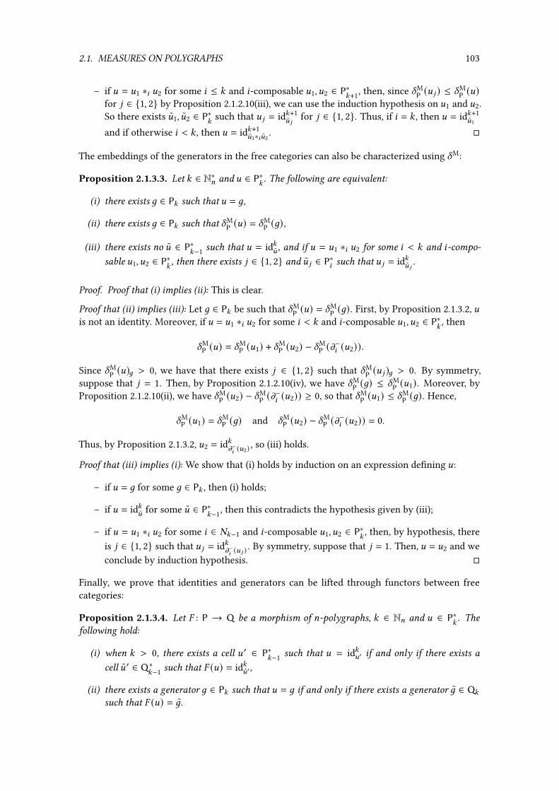
2.1. MEASURES ON POLYGRAPHS 103

– if D = D1 ∗8 D2 for some 8 ≤ : and 8-composable D1, D2 ∈ P∗:+1, then, since XMP (D 9 ) ≤ X

MP (D)

for 9 ∈ {1, 2} by Proposition 2.1.2.10(iii), we can use the induction hypothesis on D1 and D2.So there exists D1, D2 ∈ P∗: such that D 9 = id:+1D 9

for 9 ∈ {1, 2}. Thus, if 8 = : , then D = id:+1D1

and if otherwise 8 < : , then D = id:+1D1∗8D2. �

The embeddings of the generators in the free categories can also be characterized using XM:

Proposition 2.1.3.3. Let : ∈ N∗= and D ∈ P∗: . The following are equivalent:

(i) there exists 6 ∈ P: such that D = 6,

(ii) there exists 6 ∈ P: such that XMP (D) = X

MP (6),

(iii) there exists no D ∈ P∗:−1 such that D = id:D , and if D = D1 ∗8 D2 for some 8 < : and 8-compo-

sable D1, D2 ∈ P∗: , then there exists 9 ∈ {1, 2} and D 9 ∈ P∗8 such that D 9 = id:D 9 .

Proof. Proof that (i) implies (ii): This is clear.

Proof that (ii) implies (iii): Let 6 ∈ P: be such that XMP (D) = X

MP (6). First, by Proposition 2.1.3.2, D

is not an identity. Moreover, if D = D1 ∗8 D2 for some 8 < : and 8-composable D1, D2 ∈ P∗: , then

XMP (D) = X

MP (D1) + XM

P (D2) − XMP (m

−8 (D2)).

Since XMP (D)6 > 0, we have that there exists 9 ∈ {1, 2} such that XM

P (D 9 )6 > 0. By symmetry,suppose that 9 = 1. Then, by Proposition 2.1.2.10(iv), we have XM

P (6) ≤ XMP (D1). Moreover, by

Proposition 2.1.2.10(ii), we have XMP (D2) − XM

P (m−8 (D2)) ≥ 0, so that XM

P (D1) ≤ XMP (6). Hence,

XMP (D1) = XM

P (6) and XMP (D2) − XM

P (m−8 (D2)) = 0.

Thus, by Proposition 2.1.3.2, D2 = id:m−8(D2) , so (iii) holds.

Proof that (iii) implies (i): We show that (i) holds by induction on an expression de�ning D:

– if D = 6 for some 6 ∈ P: , then (i) holds;

– if D = id:D for some D ∈ P∗:−1, then this contradicts the hypothesis given by (iii);

– if D = D1 ∗8 D2 for some 8 ∈ #:−1 and 8-composable D1, D2 ∈ P∗: , then, by hypothesis, thereis 9 ∈ {1, 2} such that D 9 = id:

m−8(D 9 ) . By symmetry, suppose that 9 = 1. Then, D = D2 and we

conclude by induction hypothesis. �

Finally, we prove that identities and generators can be lifted through functors between freecategories:

Proposition 2.1.3.4. Let � : P → Q be a morphism of =-polygraphs, : ∈ N= and D ∈ P∗:. The

following hold:

(i) when : > 0, there exists a cell D ′ ∈ P∗:−1 such that D = id:D′ if and only if there exists a

cell D ′ ∈ Q∗:−1 such that � (D) = id:D′ ,

(ii) there exists a generator 6 ∈ P: such that D = 6 if and only if there exists a generator 6 ∈ Q:such that � (D) = 6.

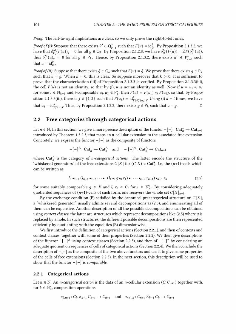
104 CHAPTER 2. THE WORD PROBLEM ON STRICT CATEGORIES

Proof. The left-to-right implications are clear, so we only prove the right-to-left ones.

Proof of (i): Suppose that there exists D ′ ∈ Q∗:−1 such that � (D) = id:D′ . By Proposition 2.1.3.2, we

have that XMQ (� (D))6 = 0 for all 6 ∈ Q: . By Proposition 2.1.2.8, we have XM

Q (� (D)) = Z� (XMP (D)),

thus XMP (D)6 = 0 for all 6 ∈ P: . Hence, by Proposition 2.1.3.2, there exists D ′ ∈ P∗

:−1 suchthat D = id:D′ .

Proof of (ii): Suppose that there exists 6 ∈ Q: such that � (D) = 6. We prove that there exists 6 ∈ P:such that D = 6. When : = 0, this is clear. So suppose moreover that : > 0. It is su�cient toprove that the characterization (iii) of Proposition 2.1.3.3 is veri�ed. By Proposition 2.1.3.3(iii),the cell � (D) is not an identity, so that by (i), D is not an identity as well. Now if D = D1 ∗8 D2for some 8 ∈ N:−1 and 8-composable D1, D2 ∈ P∗

:, then � (D) = � (D1) ∗8 � (D2), so that, by Propo-

sition 2.1.3.3(iii), there is 9 ∈ {1, 2} such that � (D 9 ) = id:� (m−

8(D 9 )) . Using (i) : − 8 times, we have

that D 9 = id:m−8(D 9 ) . Thus, by Proposition 2.1.3.3, there exists 6 ∈ P: such that D = 6. �

2.2 Free categories through categorical actions

Let = ∈ N. In this section, we give a more precise description of the functor −[−] : Cat+= → Cat=+1introduced by Theorem 1.3.2.3, that maps an =-cellular extension to the associated free extension.Concretely, we express the functor −[−] as the composite of functors

−[−]A : Cat+= → CatA= and − [−]≈ : CatA= → Cat=+1

where CatA= is the category of =-categorical actions. The latter encode the structure of the“whiskered generators” of the free extensions � [- ] for (�,- ) ∈ Cat+= , i.e., the (=+1)-cells whichcan be written as

;= r=−1 (;=−1 r

=−2 · · · r1 (;1 r0 6 r0 A1) r1 · · · r=−2 A=−1) r=−1 A= (2.5)

for some suitably composable 6 ∈ - and ;8 , A8 ∈ �8 for 8 ∈ N∗= . By considering adequatelyquotiented sequences of (=+1)-cells of such form, one recovers the whole set � [- ]=+1.

By the exchange condition (E) satis�ed by the canonical precategorical structure on � [- ],a “whiskered generator” usually admits several decompositions as (2.5), and enumerating all ofthem can be expensive. Another description of all the possible decompositions can be obtainedusing context classes: the latter are structures which represent decompositions like (2.5) where 6 isreplaced by a hole. In such structures, the di�erent possible decompositions are then representede�ciently by quotienting with the equalities (E) dimensionwise.

We �rst introduce the de�nition of categorical actions (Section 2.2.1), and then of contexts andcontext classes, together with some of their properties (Section 2.2.2). We then give descriptionsof the functor −[−]A using context classes (Section 2.2.3), and then of −[−]≈ by considering anadequate quotient on sequences of cells of categorical actions (Section 2.2.4). We then conclude thedescription of −[−] as the composite of the two above functors and use it to give some propertiesof the cells of free extensions (Section 2.2.5). In the next section, this description will be used toshow that the functor −[−] is computable.

2.2.1 Categorical actions

Let = ∈ N. An =-categorical action is the data of an =-cellular extension (�,�=+1) together with,for : ∈ N∗= , composition operations

r:,=+1 : �: ×:−1 �=+1 → �=+1 and r

=+1,: : �=+1 ×:−1 �: → �=+1

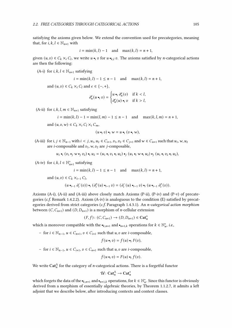
2.2. FREE CATEGORIES THROUGH CATEGORICAL ACTIONS 105

satisfying the axioms given below. We extend the convention used for precategories, meaningthat, for 8, :, ; ∈ N=+1 with

8 = min(:, ;) − 1 and max(:, ;) = = + 1,

given (D, E) ∈ �: ×8 �; , we write D r8 E for D r

:,; E . The axioms satis�ed by =-categorical actionsare then the following:

(A-i) for 8, :, ; ∈ N=+1 satisfying

8 = min(:, ;) − 1 ≤ = − 1 and max(:, ;) = = + 1,

and (D, E) ∈ �: ×8 �; and n ∈ {−, +},

mn= (D r8 E) =

{D r

8 mn= (E) if : < ; ,

mn= (D) r8 E if : > ; ,

(A-ii) for 8, :, ;,< ∈ N=+1 satisfying

8 = min(:, ;) − 1 = min(;,<) − 1 ≤ = − 1 and max(:, ;,<) = = + 1,

and (D, E,F) ∈ �: ×8 �; ×8 �< ,

(D r8 E) r8 F = D r

8 (E r8 F),

(A-iii) for 8, 9 ∈ N=−1 with 8 < 9 ,D1, D2 ∈ �8+1, E1, E2 ∈ � 9+1 andF ∈ �=+1 such thatD1,F,D2are 8-composable and E1,F, E2 are 9-composable,

D1 r8 (E1 r

9 F r9 E2) r8 D2 = (D1 r

8 E1 r8 D2) r9 (D1 r

8 F r8 D2) r9 (D1 r

8 E2 r8 D2),

(A-iv) for 8, :, ; ∈ N∗=+1 satisfying

8 = min(:, ;) − 1 ≤ = − 1 and max(:, ;) = = + 1,

and (D, E) ∈ �: ×8−1 �; ,

(D r8−1 m

−8 (E)) r8 (m+8 (D) r8−1 E) = (m−8 (D) r8−1 E) r8 (D r

8−1 m+8 (E)) .

Axioms (A-i), (A-ii) and (A-iii) above closely match Axioms (P-ii), (P-iv) and (P-v) of precate-gories (c.f. Remark 1.4.2.2). Axiom (A-iv) is analoguous to the condition (E) satis�ed by precat-egories derived from strict categories (c.f. Paragraph 1.4.3.1). An =-categorical action morphismbetween (�,�=+1) and (�, �=+1) is a morphism of =-cellular extension

(�, 5 ) : (�,�=+1) → (�,�=+1) ∈ Cat+=which is moreover compatible with the r

:,=+1 and r=+1,: operations for : ∈ N∗= , i.e.,

– for 8 ∈ N=−1, D ∈ �=+1, E ∈ �8+1 such that D, E are 8-composable,

5 (D r8 E) = 5 (D) r8 � (E),

– for 8 ∈ N=−1, D ∈ �8+1, E ∈ �=+1 such that D, E are 8-composable,

5 (D r8 E) = � (D) r8 5 (E) .

We write CatA= for the category of =-categorical actions. There is a forgetful functor

U : CatA= → Cat+=which forgets the data of the r

:,=+1 and r=+1,: operations, for : ∈ N∗= . Since this functor is obviously

derived from a morphism of essentially algebraic theories, by Theorem 1.1.2.7, it admits a leftadjoint that we describe below, after introducing contexts and context classes.

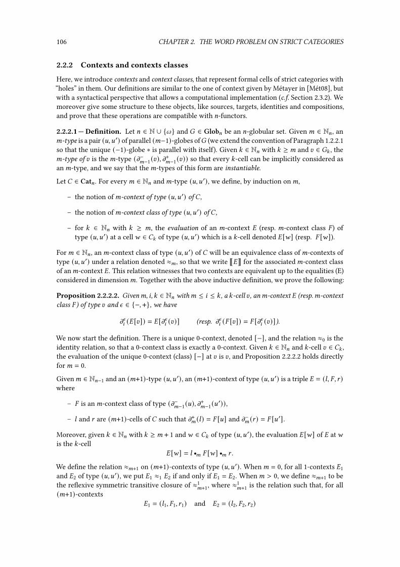
106 CHAPTER 2. THE WORD PROBLEM ON STRICT CATEGORIES

2.2.2 Contexts and contexts classes

Here, we introduce contexts and context classes, that represent formal cells of strict categories with“holes” in them. Our de�nitions are similar to the one of context given by Métayer in [Mét08], butwith a syntactical perspective that allows a computational implementation (c.f. Section 2.3.2). Wemoreover give some structure to these objects, like sources, targets, identities and compositions,and prove that these operations are compatible with =-functors.

2.2.2.1 — De�nition. Let = ∈ N ∪ {l} and � ∈ Glob= be an =-globular set. Given< ∈ N= , an<-type is a pair (D,D ′) of parallel (<−1)-globes of� (we extend the convention of Paragraph 1.2.2.1so that the unique (−1)-globe ∗ is parallel with itself). Given : ∈ N= with : ≥ < and E ∈ �: , the<-type of E is the<-type (m−<−1(E), m+<−1(E)) so that every :-cell can be implicitly considered asan<-type, and we say that the<-types of this form are instantiable.

Let � ∈ Cat= . For every< ∈ N= and<-type (D,D ′), we de�ne, by induction on<,

– the notion of<-context of type (D,D ′) of � ,

– the notion of<-context class of type (D,D ′) of � ,

– for : ∈ N= with : ≥ <, the evaluation of an <-context � (resp. <-context class � ) oftype (D,D ′) at a cellF ∈ �: of type (D,D ′) which is a :-cell denoted � [F] (resp. � [F]).

For< ∈ N= , an<-context class of type (D,D ′) of � will be an equivalence class of<-contexts oftype (D,D ′) under a relation denoted ≈< , so that we write È�É for the associated<-context classof an<-context �. This relation witnesses that two contexts are equivalent up to the equalities (E)considered in dimension<. Together with the above inductive de�nition, we prove the following:

Proposition 2.2.2.2. Given<, 8, : ∈ N= with< ≤ 8 ≤ : , a :-cell E , an<-context � (resp.<-contextclass � ) of type E and n ∈ {−, +}, we have

mn8 (� [E]) = � [mn8 (E)] (resp. mn8 (� [E]) = � [mn8 (E)]).

We now start the de�nition. There is a unique 0-context, denoted [−], and the relation ≈0 is theidentity relation, so that a 0-context class is exactly a 0-context. Given : ∈ N= and :-cell E ∈ �: ,the evaluation of the unique 0-context (class) [−] at E is E , and Proposition 2.2.2.2 holds directlyfor< = 0.

Given< ∈ N=−1 and an (<+1)-type (D,D ′), an (<+1)-context of type (D,D ′) is a triple � = (;, � , A )where

– � is an<-context class of type (m−<−1(D), m+<−1(D ′)),

– ; and A are (<+1)-cells of � such that m+< (;) = � [D] and m−< (A ) = � [D ′].

Moreover, given : ∈ N= with : ≥ < + 1 andF ∈ �: of type (D,D ′), the evaluation � [F] of � atFis the :-cell

� [F] = ; r< � [F] r< A .We de�ne the relation ≈<+1 on (<+1)-contexts of type (D,D ′). When< = 0, for all 1-contexts �1and �2 of type (D,D ′), we put �1 ≈1 �2 if and only if �1 = �2. When< > 0, we de�ne ≈<+1 to bethe re�exive symmetric transitive closure of ≈1

<+1, where ≈1<+1 is the relation such that, for all

(<+1)-contexts�1 = (;1, �1, A1) and �2 = (;2, �2, A2)

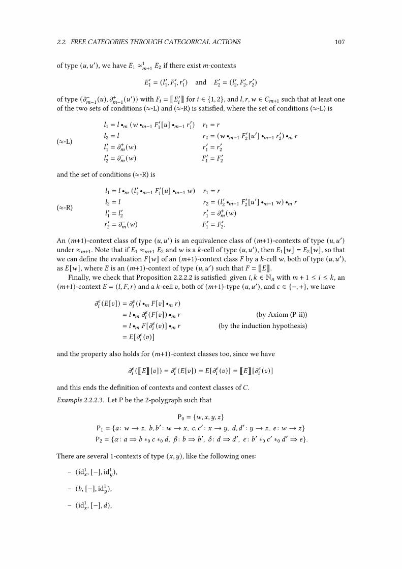
2.2. FREE CATEGORIES THROUGH CATEGORICAL ACTIONS 107

of type (D,D ′), we have �1 ≈1<+1 �2 if there exist<-contexts

� ′1 = (; ′1, � ′1, A ′1) and � ′2 = (; ′2, � ′2, A ′2)

of type (m−<−1(D), m+<−1(D ′)) with �8 = È� ′8É for 8 ∈ {1, 2}, and ;, A ,F ∈ �<+1 such that at least oneof the two sets of conditions (≈-L) and (≈-R) is satis�ed, where the set of conditions (≈-L) is

(≈-L)

;1 = ; r< (F r<−1 �

′1 [D] r<−1 A

′1) A1 = A

;2 = ; A2 = (F r<−1 �

′2 [D ′] r<−1 A

′2) r< A

; ′1 = m+< (F) A ′1 = A

′2

; ′2 = m−< (F) � ′1 = �

′2

and the set of conditions (≈-R) is

(≈-R)

;1 = ; r< (; ′1 r<−1 �

′1 [D] r<−1 F) A1 = A

;2 = ; A2 = (; ′2 r<−1 �

′2 [D ′] r<−1 F) r< A

; ′1 = ;′2 A ′1 = m

+< (F)

A ′2 = m−< (F) � ′1 = �

′2.

An (<+1)-context class of type (D,D ′) is an equivalence class of (<+1)-contexts of type (D,D ′)under ≈<+1. Note that if �1 ≈<+1 �2 andF is a :-cell of type (D,D ′), then �1 [F] = �2 [F], so thatwe can de�ne the evaluation � [F] of an (<+1)-context class � by a :-cellF , both of type (D,D ′),as � [F], where � is an (<+1)-context of type (D,D ′) such that � = È�É.

Finally, we check that Proposition 2.2.2.2 is satis�ed: given 8, : ∈ N= with< + 1 ≤ 8 ≤ : , an(<+1)-context � = (;, � , A ) and a :-cell E , both of (<+1)-type (D,D ′), and n ∈ {−, +}, we have

mn8 (� [E]) = mn8 (; r< � [E] r< A )= ; r< mn8 (� [E]) r< A (by Axiom (P-ii))= ; r< � [mn8 (E)] r< A (by the induction hypothesis)= � [mn8 (E)]

and the property also holds for (<+1)-context classes too, since we have

mn8 (È�É[E]) = mn8 (� [E]) = � [mn8 (E)] = È�É[mn8 (E)]

and this ends the de�nition of contexts and context classes of � .

Example 2.2.2.3. Let P be the 2-polygraph such that

P0 = {F, G,~, I}P1 = {0 : F → I, 1, 1 ′ : F → G, 2, 2 ′ : G → ~, 3, 3 ′ : ~ → I, 4 : F → I}P2 = {U : 0 ⇒ 1 ∗0 2 ∗0 3, V : 1 ⇒ 1 ′, X : 3 ⇒ 3 ′, n : 1 ′ ∗0 2 ′ ∗0 3 ′⇒ 4}.

There are several 1-contexts of type (G,~), like the following ones:

– (id1G , [−], id1

~),

– (1, [−], id1~),

– (id1G , [−], 3),

108 CHAPTER 2. THE WORD PROBLEM ON STRICT CATEGORIES

�1 = F G ~ I

0

4

1

1 ′

2

2 ′

3

3 ′⇓V ⇓X

⇓U

⇓n

�2 = F G ~ I

0

4

1

1 ′

2

2 ′

3

3 ′⇓V ⇓X

⇓U

⇓n

�3 = F G ~ I

0

4

1

1 ′

2

2 ′

3

3 ′⇓V ⇓X

⇓U

⇓n

�4 = F G ~ I

0

4

1

1 ′

2

2 ′

3

3 ′⇓V ⇓X

⇓U

⇓n

Figure 2.1 – The contexts �1, �2, �3 and �4

– �5 ,ℎ = (5 , [−], 6) for 5 ∈ {1,1 ′} and ℎ ∈ {3, 3 ′}.

By the de�nition of ≈1, a 1-context class is exactly a 1-context. Note that, for 5 ∈ {1, 1 ′}and ℎ ∈ {2, 2 ′}, the evaluation of �5 ,ℎ at 6 ∈ {2, 2 ′} is 5 ∗0 6 ∗0 ℎ. There are several 2-contexts oftype (2, 2 ′), as the following ones:

– �1 = (U ∗1 (V ∗0 id22 ∗0 X), �1′,3′, n),

– �2 = (U ∗1 (id21∗02 ∗0 X), �1,3′, (V ∗0 id2

2′∗03′) ∗1 n),

– �3 = (U ∗1 (V ∗0 id22∗03 ), �1′,3 , (id

21′∗02′ ∗0 X) ∗1 n),

– �4 = (U, �1,3 , (V ∗0 id22′ ∗0 X) ∗1 n)

which can be represented as on Figure 2.1. Then, putting

; = U ∗1 (id21∗02 ∗0 X), F = V and A = n

and using (≈-L), we have �1 ≈12 �2. Similarly, putting

; = U ∗1 (V ∗0 id22∗03 ), F = X and A = n

and using (≈-R), we have �1 ≈1< �3. Finally, putting

; = U, F = X and A = (V ∗0 id22′∗03′) ∗1 n

and using (≈-R), we have �2 ≈1< �4. Thus, we have

È�1É = È�2É = È�3É = È�4É.

In fact, we can prove that the set of 2-contexts equivalent to �1 under ≈2 is {�1, �2, �3, �4}.

2.2. FREE CATEGORIES THROUGH CATEGORICAL ACTIONS 109

Remark 2.2.2.4. Given< ∈ N= , the relation ≈−1< on the<-contexts, which is de�ned by �1 ≈−1

< �2when �2 ≈1

< �1 for all<-contexts �1, �2 of the same<-type, admits a de�nition by axioms (≈-L)’and (≈-R)’ which are symmetrical to (≈-L) and (≈-R). Moreover, ≈< can be equivalently describedas the re�exive transitive closure of ≈1

<∪≈−1< , so that, in the proofs, by symmetry of the de�nitions

of ≈1< and ≈−1

< , we can often reduce a case analysis of �1 ≈< �2 to �1 ≈1< �2.

Remark 2.2.2.5. Given <,: ∈ N=+1 with < ≤ = and < ≤ : ≤ = + 1, the notion of <-context,<-context class and their respective evaluations at a :-cell can be de�ned similarly for an =-cate-gorical action � . Note that the notion of (=+1)-context here makes little sense since there is nocomposition operation r

= .

2.2.2.6 — Source and target of contexts. Let = ∈ N ∪ {l} and � ∈ Cat= . Given < ∈ N∗= , an<-type (D,D ′) and an<-context � = (;, � , A ) of type (D,D ′) of� , the source and the target of � arerespectively the (<−1)-cells

m−<−1(�) = m−<−1(;) and m+<−1(�) = m+<−1(A ).

When< > 1, we moreover have

mn<−2 ◦ m−<−1(�) = mn<−2 ◦ m+<−1(�)

for n ∈ {−, +}. Indeed, given an (<−1)-context � ′ = (; ′, � ′, A ′) such that � = È� ′É, we have

m+(;) = ; ′ r<−2 �′[D] r<−2 A

′ and m−(A ) = ; ′ r<−2 �′[D ′] r<−2 A

′

so that

m−<−2 ◦ m−<−1(�) = m−<−2 ◦ m−<−1(;)= m−<−2 ◦ m+<−1(;)= m−<−2(; ′)= m−<−2 ◦ m−<−1(A )= m−<−2 ◦ m+<−1(A )= m−<−2 ◦ m+<−1(�)

and similarly, m+<−2 ◦ m−<−1(�) = m+<−2 ◦ m+<−1(�). The operations m−, m+ on<-contexts extend to<-context classes since they are compatible with the ≈< relation. Given 8 ∈ N<−1 and n ∈ {−, +}and an<-context � (resp. an<-context class � ), we write mn8 (�) for mn8 ◦mn<−1(�) (resp. mn8 ◦mn<−1(� )).Thus, for 8 ∈ N=−1, we can extend the notion of 8-composable sequences of globes of globular setsto sequences -1, . . . , -; for some ; ∈ N∗ where -B is either an<-context, an<-context class, or acell of � for B ∈ N∗

;, and say that -1, . . . , -; is 8-composable when m+8 (-B) = m−8 (-B+1) for B ∈ N∗

;−1.

It is immediate that the source and target operations are compatible with the evaluation of contexts(resp. context classes):

Proposition 2.2.2.7. Given 8,<, : ∈ N= with 8 < < ≤ : , n ∈ {−, +}, D ∈ �: and an<-context � oftype D, we have

mn8 (� [D]) = mn8 (�) and mn8 (È�É[D]) = mn8 (È�É).

110 CHAPTER 2. THE WORD PROBLEM ON STRICT CATEGORIES

2.2.2.8 — Identity contexts. Let = ∈ N∪{l} and� ∈ Cat= . Given< ∈ N= and an<-type (D,D ′)of � , we de�ne an <-context � (D,D′) and an <-context class � (D,D′) , called respectively identitycontext and identity context class on (D,D ′), by induction on<. When< = 0, we put

� (∗,∗) = � (∗,∗) = [−]

and, when< > 0, we put

� (D,D′) = (id<D , � (m

− (D),m+ (D′)) , id<D′) and � (D,D′) = È� (D,D′)É.

If � is part of an =-cellular extension (�,- ), given 6 ∈ - , we write �6 and �6 for

� (m−=−1 (6),m+=−1 (6)) and � (m

−=−1 (6),m+=−1 (6))

respectively. The identity contexts and identity context classes have trivial evaluation:

Proposition 2.2.2.9. For<,: ∈ N= with< ≤ : , an<-type (D,D ′) and E ∈ �: of type (D,D ′), wehave

� (D,D′) [E] = E and � (D,D

′) [E] = E

Proof. This is shown by a simple induction on<. �

2.2.2.10 — Composition operations. Let= ∈ N∪{l} and� ∈ Cat= . Given 8,< ∈ N= with 8 < <,an<-context � = (;, � , A ) of some<-type (D,D ′) of � , and E ∈ �8+1, if (E, �) is 8-composable, wede�ne an<-context E r

8 � by induction on< − 8 with

E r8 � =

{(E r

8 ;, � , A ) if 8 + 1 =<,(E r

8 ;, E r8 �, E r

8 A ) if 8 + 1 < <,

and, since it can be veri�ed that the r8 operation is compatible with ≈< , we extend the operation

on<-context classes and put E r8 È�É = ÈE r

8 �É. Similarly, if (�, E) is 8-composable, we de�ne an<-context � r

8 E using an induction on< − 8 by

� r8 E =

{(;, � , A r

8 E) if 8 + 1 =<,(; r8 E, � r

8 E, A r8 E) if 8 + 1 < <,

and we put È�É r8 E = È� r

8 EÉ. These composition operations satisfy properties similar to theaxioms of (=+1)-precategories:

Proposition 2.2.2.11. Given< ∈ N= , an<-type (D,D ′) and an<-context � of type (D,D ′) of � ,we have

(i) for all 8 ∈ N<−1 and D1 = m−8 (�), D2 = m

+8 (�),

id8+1D1r8 � = � = � r

8 id8+1D2 ,

(ii) for all 8 ∈ N<−1 and D1, D2 ∈ �8+1, if D1, D2, � are 8-composable or D1, �,D2 are 8-composableor �,D1, D2 are 8-composable, then we respectively have

(D1 r8 D2) r8 � = D1 r

8 (D2 r8 �)

or

(D1 r8 �) r8 D2 = D1 r

8 (� r8 D2)

or

(� r8 D1) r8 D2 = � r

8 (D1 r8 D2),

2.2. FREE CATEGORIES THROUGH CATEGORICAL ACTIONS 111

(iii) for all 8, 9 ∈ N<−1 such that 8 < 9 , and D1, D2 ∈ �8+1 and E1, E2 ∈ � 9+1 such that D1, �,D2 are8-composable and E1, �, E2 are 9-composable, we have

D1 r8 (E1 r

9 � r9 E2) r8 D2 = (D1 r

8 E1 r8 D2) r9 (D1 r

8 � r8 D2) r9 (D1 r

8 E2 r8 D2),

and similar properties hold when replacing � by È�É in the equations.

Proof. (i), (ii) are proved by a simple induction on � and � , so we move directly to the proof of (iii).Let (;, � , A ) = �, 8, 9 ∈ N<−1 with 8 < 9 , and D1, D2 ∈ �8+1 and E1, E2 ∈ � 9+1 such that D1, �,D2are 8-composable and E1, �, E2 are 9-composable. We show that (iii) holds by induction on< − 9 .When< = 9 + 1, we have

D1 r8 (E1 r

9 � r9 E2) r8 D2 = (D1 r

8 (E1 r9 ;) r8 D2, � ,D1 r

8 (A r9 E2) r8 D2)

= ((D1 r8 E1 r

8 D2) r9 (D1 r8 ; r8 D2), � , (D1 r

8 A r8 D2) (D1 r

8 E2 r8 D2))

= (D1 r8 E1 r

8 D2) r9 (D1 r8 � r

8 D2) r9 (D1 r8 E2 r

8 D2)and moreover,

D1 r8 (E1 r

9 È�É r9 E2) r8 D2 = ÈD1 r

8 (E1 r9 � r

9 E2) r8 D2É= È(D1 r

8 E1 r8 D2) r9 (D1 r

8 � r8 D2) r9 (D1 r

8 E2 r8 D2)É

= (D1 r8 E1 r

8 D2) r9 (D1 r8 È�É r

8 D2) r9 (D1 r8 E2 r

8 D2)so that the wanted equations hold. When< > 9 +1, by doing a similar computation and using theinduction hypothesis on � , we conclude that the wanted equations hold too. Thus, (iii) holds. �

Moreover, by the axioms de�ning the relations ≈< , the compositions of cells of � with contextclasses satisfy an equality similar to the condition (E) that characterizes =-categories among=-precategories:

Proposition 2.2.2.12. Given 8,< ∈ N= with 0 < 8 < <, an <-type (D,D ′), an <-context � oftype (D,D ′), and D1, D2 ∈ �8+1 such that D1, � are (8−1)-composable and �,D2 are (8−1)-composable,we have

(D1 r8−1 m

−8 (È�É)) r8 (m+8 (D1) r8−1 È�É) = (m−8 (D1) r8−1 È�É) r8 (D1 r

8−1 m+8 (È�É))

and

(È�É r8−1 m

−8 (D2)) r8 (m+8 (È�É) r8−1 D2) = (m−8 (È�É) r8−1 D2) r8 (È�É r

8−1 m+8 (D2)) .

Moreover, if 8 + 1 < <, we have

(D1 r8−1 m

−8 (�)) r8 (m+8 (D1) r8−1 �) = (m−8 (D1) r8−1 �) r8 (D1 r

8−1 m+8 (�))

and

(� r8−1 m

−8 (D2)) r8 (m+8 (�) r8−1 D2) = (m−8 (�) r8−1 D2) r8 (� r

8−1 m+8 (D2)).

Proof. Let (;, � , A ) = �. We show this property by induction on< − 8 . If< = 8 + 1, then

(D1 r8−1 m

−8 (�)) r8 (m+8 (D1) r8−1 �)

= (D1 r8−1 m

−8 (;)) r8 (m+8 (D1) r8−1 �)

= ( [D1 r8−1 m

−8 (;)] r8 [m+8 (D1) r8−1 ;], m+8 (D1) r8−1 �, m

+8 (D1) r8−1 A )

= ( [m−8 (D1) r8−1 ;] r8 [D1 r8−1 m

+8 (;)], m+8 (D1) r8−1 �, m

+8 (D1) r8−1 A ) (by (E))

≈< ( [m−8 (D1) r8−1 ;], m−8 (D1) r8−1 �, [D1 r8−1 m

−8 (A )] r8 [m+8 (D1) r8−1 A ])

= ( [m−8 (D1) r8−1 ;], m−8 (D1) r8−1 �, [m−8 (D1) r8−1 A ] r8 [D1 r8−1 m

+8 (A )]) (by (E))

= (m−8 (D1) r8−1 �) r8 (D1 r8 m+8 (A ))

= (m−8 (D1) r8−1 �) r8 (D1 r8 m+8 (�))

112 CHAPTER 2. THE WORD PROBLEM ON STRICT CATEGORIES

so that

(D1 r8−1 m

−8 (È�É)) r8 (m+8 (D1) r8−1 È�É)

= È(D1 r8−1 m

−8 (�)) r8 (m+8 (D1) r8−1 �)É

= È(m−8 (D1) r8−1 �) r8 (D1 r8 m+8 (�))É

= (m−8 (D1) r8−1 È�É) r8 (D1 r8 m+8 (È�É))

and similarly,

(È�É r8−1 m

−8 (D2)) r8 (m+8 (È�É) r8−1 D2) = (m−8 (È�É) r8−1 D2) r8 (È�É r

8−1 m+8 (D2)) .

Otherwise, if< > 8 + 1, then

(D1 r8−1 m

−8 (�)) r8 (m+8 (D1) r8−1 ;)

= (D1 r8−1 m

−8 (;)) r8 (m+8 (D1) r8−1 ;)

= (m−8 (D1) r8−1 ;) r8 (D1 r8−1 m

+8 (;))

= (m−8 (D1) r8−1 ;) r8 (D1 r8−1 m

+8 (�))

and similarly,

(D1 r8−1 m

−8 (�)) r8 (m+8 (D1) r8−1 A ) = (m−8 (D1) r8−1 A ) r8 (D1 r

8−1 m+8 (�))

and, by induction hypothesis,

(D1 r8−1 m

−8 (�)) r8 (m+8 (D1) r8−1 � )

= (D1 r8−1 m

−8 (� )) r8 (m+8 (D1) r8−1 � )

= (m−8 (D1) r8−1 � ) r8 (D1 r8−1 m

+8 (� ))

= (m−8 (D1) r8−1 � ) r8 (D1 r8−1 m

+8 (�))

so that

(D1 r8−1 m

−8 (�)) r8 (m+8 (D1) r8−1 �) = (m−8 (D1) r8−1 �) r8 (D1 r

8−1 m+8 (�))

which implies(D1 r

8−1 m−8 (È�É)) r8 (m+8 (D1) r8−1 È�É) = (m−8 (D1) r8−1 È�É) r8 (D1 r

8−1 m+8 (È�É)).

Similarly, we have

(m−8 (�) r8−1 D2) r8 (� r8−1 m

+8 (D2)) = (� r

8−1 m−8 (D2)) r8 (m+8 (�) r8−1 D2)

and(È�É r

8−1 m−8 (D2)) r8 (m+8 (È�É) r8−1 D2) = (m−8 (È�É) r8−1 D2) r8 (È�É r

8−1 m+8 (D2)) .

Hence, the proposition holds. �

Finally, we prove that the composition operations on contexts and context classes are compatiblewith evaluation:

Proposition 2.2.2.13. Given 8,<, : ∈ N= with 8 < < ≤ : , D ∈ �8+1, E ∈ �: and an<-context � oftype E of � , if D, � are 8-composable, then

(D r8 �) [E] = D r

8 (� [E])

and otherwise, if �,D are 8-composable, then

(� r8 D) [E] = (� [E]) r8 D

and similar equalities hold for context classes.

2.2. FREE CATEGORIES THROUGH CATEGORICAL ACTIONS 113

Proof. By symmetry, we only prove the �rst equality, and we do so using an induction on< − 8 .Let (;, � , A ) = �. When 8 + 1 =<, we have

(D r8 �) [E] = D r

8 ; r8 � [E] r8 A = D r8 � [E]

and

(D r8 È�É)[E] = ÈD r

8 �É[E] = (D r8 �) [E] = D r

8 (� [E]) = D r8 (È�É[E]).

Otherwise, when 8 + 1 < <, we have

(D r8 �) [E] = (D r

8 ;) r<−1 (D r8 � ) [E] r<−1 (D r

8 A )= (D r

8 ;) r<−1 (D r8 (� [E])) r<−1 (D r

8 A ) (by induction hypothesis)= D r

8 (� [E])

and, like above, we have (D r8 È�É)[E] = D r

8 (È�É[E]). �

2.2.2.14 — Contexts and functoriality. Let = ∈ N ∪ {l}, �, � ∈ Cat= and � : � → � be an=-functor. We extend � to<-contexts and<-context classes, by induction on<. More precisely,given< ∈ N= , an<-type (D,D ′) of� and an<-context � of type (D,D ′) of� , we de�ne an<-con-text� (�) and an<-context class� (È�É) of type (� (D), � (D ′)) of� by induction on< as follows.If< = 0, we put

� ( [−]) = [−]

and otherwise, if< > 0, given (;, � , A ) = �, we put

� (�) = (� (;), � (� ), � (A )) and � (È�É) = È� (�)É

where � (È�É) is well-de�ned since, given two <-contexts �1, �2 such that �1 ≈< �2, we cancheck that � (�1) ≈< � (�2). We verify that � is compatible with the di�erent operations oncontexts and context classes de�ned above:

Proposition 2.2.2.15. Given<,: ∈ N= with< ≤ : , D ∈ �: and an<-context � of type D of � , wehave

� (� [D]) = � (�) [� (D)] and � (È�É[D]) = � (È�É)[� (D)]

Proof. We prove this property by induction on<. When< = 0, the property holds, so assumethat< > 0. Let (;, � , A ) = �. We have

� (� [D]) = � (;) r<−1 � (� [D]) r<−1 � (A )= � (;) r<−1 � (� ) [� (D)] r<−1 � (A ) (by induction hypothesis)= � (�) [� (D)]

and we moreover deduce that

� (È�É[D]) = � (� [D]) = � (�) [� (D)] = È� (�)É[� (D)] = � (È�É)[� (D)]

which concludes the induction. �

Proposition 2.2.2.16. Given< ∈ N= and an<-type (D,D ′) of � , we have

� (� (D,D′) ) = � (� (D),� (D′)) and � (� (D,D′) ) = � (� (D),� (D′))

114 CHAPTER 2. THE WORD PROBLEM ON STRICT CATEGORIES

Proof. By a simple induction on<. �

Proposition 2.2.2.17. Given 8,< ∈ N= with 8 < <, D ∈ �8+1 and an <-context � of � , if D, �(resp. �,D) are 8-composable, then

� (D r8 �) = � (D) r8 � (�) (resp. � (� r

8 D) = � (�) r8 � (D))and

� (D r8 È�É) = � (D) r8 � (È�É) (resp. � (È�É r

8 D) = � (È�É) r8 D).Proof. Let (;, � , A ) = �. We prove this property by induction on< − 8 . If< = 8 + 1, we computethat

� (D r8 �) = � ((D r

8 ;, � , A ))= (� (D r

8 ;), � (� ), � (A ))= (� (D) r8 � (;), � (� ), � (A ))= � (D) r8 (� (;), � (� ), � (A ))= � (D) r8 � (�)

and� (D r

8 È�É) = � (ÈD r8 �É)

= È� (D r8 �)É

= È� (D) r8 � (�)É= � (D) r8 È� (�)É= � (D) r8 � (È�É).

When < > 8 + 1, an analogous computation using the induction hypothesis shows the sameequalities. The case of composition on the right is similar. �

2.2.3 Free action on a cellular extension

In this section, we use the formalism of contexts and contexts classes to de�ne a left adjoint tothe functorU : CatA= → Cat+= . In the process, we give su�cient conditions for a monomorphismto be preserved by the free action functor −[−]A : Cat+= → CatA= introduced above. Indeed, theimage of a monomorphism (�, 5 ) by −[−]A does not have to be a monomorphism since � isnot necessarily injective on contexts and contexts classes, because of the quotients with therelations ≈< . As shown below, it is su�cient to require moreover that � is a Conduché functor :those are the morphisms of Cat= that uniquely “lift compositions of cells”. Consequently, they arebetter behaved regarding the relations ≈< on contexts. We refer the reader to [Gue20] for a moreextensive presentation of Conduché functors for strict=-categories. The resulting monomorphismpreservation result of −[−]A will be useful when showing that the word problem on generalpolygraphs reduces to the one on �nite polygraphs (c.f. Section 2.4.3).

2.2.3.1 — (n+1)-categorical action structure. Let = ∈ N. Given an =-cellular extension (�,- ),we de�ne an =-categorical action � [- ]A = (�,-A) as follows: -A is the set of pairs (6, � )with 6 ∈ - and � an =-context class of type 6. The =-source and =-target of such a pair (6, � ) arede�ned respectively as the =-cells

m−= ((6, � )) = � [d−= (6)] and m+= ((6, � )) = � [d+= (6)] .

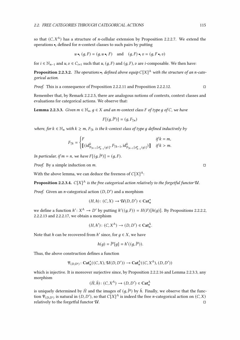
2.2. FREE CATEGORIES THROUGH CATEGORICAL ACTIONS 115

so that (�,-A) has a structure of =-cellular extension by Proposition 2.2.2.7. We extend theoperations r

8 de�ned for =-context classes to such pairs by putting

D r8 (6, � ) = (6,D r

8 � ) and (6, � ) r8 E = (6, � r8 E)

for 8 ∈ N=−1 and D, E ∈ �8+1 such that D, (6, � ) and (6, � ), E are 8-composable. We then have:

Proposition 2.2.3.2. The operations r8 de�ned above equip � [- ]A with the structure of an =-cate-

gorical action.

Proof. This is a consequence of Proposition 2.2.2.11 and Proposition 2.2.2.12. �

Remember that, by Remark 2.2.2.5, there are analogous notions of contexts, context classes andevaluations for categorical actions. We observe that:

Lemma 2.2.3.3. Given< ∈ N= , 6 ∈ - and an<-context class � of type 6 of � , we have

� [(6, �6)] = (6, �↑=)

where, for : ∈ N= with : ≥ <, �↑: is the :-context class of type 6 de�ned inductively by

�↑: =

{� if : =<,È(id:

�↑:−1 [m−:−1 (6) ], �↑:−1, id:�↑:−1 [m+:−1 (6) ]

)É if : > <.

In particular, if< = =, we have � [(6, �6)] = (6, � ).

Proof. By a simple induction on<. �

With the above lemma, we can deduce the freeness of � [- ]A:

Proposition 2.2.3.4. � [- ]A is the free categorical action relatively to the forgetful functorU.

Proof. Given an =-categorical action (�, � ′) and a morphism

(�,ℎ) : (�,- ) → U(�,� ′) ∈ Cat+=

we de�ne a function ℎ′ : -A → � ′ by putting ℎ′((6, � )) = � (� ) [ℎ(6)]. By Propositions 2.2.2.2,2.2.2.13 and 2.2.2.17, we obtain a morphism

(�,ℎ′) : (�,-A) → (�,� ′) ∈ CatA= .

Note that ℎ can be recovered from ℎ′ since, for 6 ∈ - , we have

ℎ(6) = �6 [6] = ℎ′((6, �6)).

Thus, the above construction de�nes a function

Ψ(�,�′) : Cat+= ((�,- ),U(�, � ′)) → CatA= ((�,-A), (�, � ′))

which is injective. It is moreover surjective since, by Proposition 2.2.2.16 and Lemma 2.2.3.3, anymorphism

(�, ℎ) : (�,-A) → (�,� ′) ∈ CatA=is uniquely determined by � and the images of (6, �6) by ℎ. Finally, we observe that the func-tion Ψ(�,�′) is natural in (�, � ′), so that � [- ]A is indeed the free =-categorical action on (�,- )relatively to the forgetful functorU. �

116 CHAPTER 2. THE WORD PROBLEM ON STRICT CATEGORIES

The construction (�,- ) ↦→ � [- ]A of the above proof uniquely extends to a functor

−[−]A : Cat+= → CatA=

which is left adjoint to U. Given (�,ℎ) : (�,- ) → (�,. ) in Cat+= , the =-categorical actionmorphism

� [ℎ]A : � [- ]A → � [. ]A ∈ CatA=is de�ned by

� [ℎ]A8 = �8 and � [ℎ]A=+1((6, � )) = (ℎ(6), � (� ))

for 8 ∈ N= and (6, � ) ∈ -A.

2.2.3.5 — Conduché functors. We now introduce Conduché functors, following the de�nitiongiven in [Gue20]. Let = ∈ N ∪ {l}, �, � ∈ Cat= and � : � → � be an =-functor. We say that � is=-Conduché when it satis�es that, for all 8, : ∈ N= with 8 < : , D ∈ �: , 8-composable E1, E2 ∈ �:such that � (D) = E1 ∗8 E2, there exist unique 8-composable D1, D2 ∈ �: such that

� (D1) = E1 and � (D2) = E2 and D1 ∗8 D2 = D.

The Conduché property implies a unique lifting of identities:

Proposition 2.2.3.6. If � : � → � is =-Conduché, then given 8, : ∈ N= with 8 < : , D ∈ �: ,and E ∈ �8 such that � (D) = id:E , there exists a unique D ′ ∈ �8 such that

� (D ′) = E and D = id:D′

Proof. We have � (D) = id:E = id:E ∗8 id:E and D can be factorized as id:m−8(D) ∗8 D and D ∗8 id:

m+8(D) .

Moreover,� (id:

m−8(D) ) = id:

� (m−8(D)) = id:

m−8(� (D)) = id:E

and similarly,� (id:

m+8(D) ) = id:E

so that, since � is =-Conduché, D = id:m−8(D) . Finally, if D = id:D′ for some D ′ ∈ �8 , then D ′ = m−8 (D),

which shows unicity. �

We can moreover characterize � as an =-Conduché using the precategorical structure of� and � :

Proposition 2.2.3.7. The =-functor � is =-Conduché if and only if for all 8, :1, :2, : ∈ N= with

8 = min(:1, :2) − 1 and : = max(:1, :2),

and cells D ∈ �: , E1 ∈ �:1 , E2 ∈ �:2 such that E1, E2 are 8-composable and � (D) = E1 r8 E2, there exist

unique D1 ∈ �:1 and D2 ∈ �:2 such that D1, D2 are 8-composable and

� (D1) = E1, � (D2) = E2 and D1 r8 D2 = D.

Proof. Suppose that � is =-Conduché and let 8, :1, :2, : ∈ N= satisfying

8 = min(:1, :2) − 1 and : = max(:1, :2),

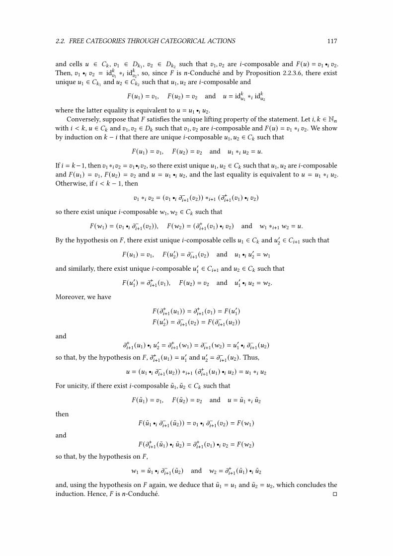
2.2. FREE CATEGORIES THROUGH CATEGORICAL ACTIONS 117

and cells D ∈ �: , E1 ∈ �:1 , E2 ∈ �:2 such that E1, E2 are 8-composable and � (D) = E1 r8 E2.

Then, E1 r8 E2 = id:E1 ∗8 id:E2 , so, since � is =-Conduché and by Proposition 2.2.3.6, there exist

unique D1 ∈ �:1 and D2 ∈ �:2 such that D1, D2 are 8-composable and

� (D1) = E1, � (D2) = E2 and D = id:D1 ∗8 id:D2

where the latter equality is equivalent to D = D1 r8 D2.

Conversely, suppose that � satis�es the unique lifting property of the statement. Let 8, : ∈ N=with 8 < : , D ∈ �: and E1, E2 ∈ �: such that E1, E2 are 8-composable and � (D) = E1 ∗8 E2. We showby induction on : − 8 that there are unique 8-composable D1, D2 ∈ �: such that

� (D1) = E1, � (D2) = E2 and D1 ∗8 D2 = D.

If 8 = :−1, then E1 ∗8 E2 = E1 r8 E2, so there exist uniqueD1, D2 ∈ �: such thatD1, D2 are 8-composable

and � (D1) = E1, � (D2) = E2 and D = D1 r8 D2, and the last equality is equivalent to D = D1 ∗8 D2.

Otherwise, if 8 < : − 1, then

E1 ∗8 E2 = (E1 r8 m−8+1(E2)) ∗8+1 (m+8+1(E1) r8 E2)

so there exist unique 8-composableF1,F2 ∈ �: such that

� (F1) = (E1 r8 m−8+1(E2)), � (F2) = (m+8+1(E1) r8 E2) and F1 ∗8+1 F2 = D.

By the hypothesis on � , there exist unique 8-composable cells D1 ∈ �: and D ′2 ∈ �8+1 such that

� (D1) = E1, � (D ′2) = m−8+1(E2) and D1 r8 D′2 = F1

and similarly, there exist unique 8-composable D ′1 ∈ �8+1 and D2 ∈ �: such that

� (D ′1) = m+8+1(E1), � (D2) = E2 and D ′1 r8 D2 = F2.

Moreover, we have

� (m+8+1(D1)) = m+8+1(E1) = � (D ′1)� (D ′2) = m−8+1(E2) = � (m−8+1(D2))

andm+8+1(D1) r8 D ′2 = m+8+1(F1) = m−8+1(F2) = D ′1 r

8 m−8+1(D2)

so that, by the hypothesis on � , m+8+1(D1) = D ′1 and D ′2 = m−8+1(D2). Thus,

D = (D1 r8 m−8+1(D2)) ∗8+1 (m+8+1(D1) r8 D2) = D1 ∗8 D2

For unicity, if there exist 8-composable D1, D2 ∈ �: such that

� (D1) = E1, � (D2) = E2 and D = D1 ∗8 D2

then� (D1 r

8 m−8+1(D2)) = E1 r

8 m−8+1(E2) = � (F1)

and� (m+8+1(D1) r8 D2) = m+8+1(E1) r8 E2 = � (F2)

so that, by the hypothesis on � ,

F1 = D1 r8 m−8+1(D2) and F2 = m

+8+1(D1) r8 D2

and, using the hypothesis on � again, we deduce that D1 = D1 and D2 = D2, which concludes theinduction. Hence, � is =-Conduché. �

118 CHAPTER 2. THE WORD PROBLEM ON STRICT CATEGORIES

2.2.3.8 — Conduché categorical action morphisms. Let = ∈ N. Anticipating the associatedmonomorphism preservation result for the left adjoint CatA= → Cat=+1, we need to introducea notion of Conduché morphism between =-categorical actions, so that the Conduché prop-erty will also be preserved by −[−]A. Following Proposition 2.2.3.7, given two =-categoricalactions (�,�=+1), (�,�=+1) ∈ CatA= and a morphism (�, 5 ) : (�,�=+1) → (�,�=+1) ∈ CatA= , wesay that the morphism (�, 5 ) is =-Conduché when � is =-Conduché and

(i) for all D ∈ �=+1, if 5 (D) = D ′ r8 E for some 8 ∈ N=−1, D ∈ �=+1 and E ∈ �8+1, then there existunique 8-composable D ′ ∈ �=+1 and E ∈ �8+1 such that

5 (D ′) = D ′, � (E) = E and D = D ′ r8 E ,

(ii) for all E ∈ �=+1, if 5 (E) = D r8 E′ for some 8 ∈ N=−1, D ∈ �8+1 and E ′ ∈ �=+1, then there exist

unique 8-composable D ∈ �8+1 and E ∈ �=+1 such that

� (D) = D, 5 (E ′) = E ′ and E = D r8 E′.

2.2.3.9 — Conduché functors and contexts. Let = ∈ N ∪ {l}. We now show that Conduchéfunctors have several good properties regarding contexts and context classes. First, they lift therelations ≈< that de�ne the<-context classes:

Proposition 2.2.3.10. Let � : � → � be a morphism in Cat= such that � is an =-Conduchéfunctor. Then, given< ∈ N= and an<-context �1 of � of type (D,D ′) and an<-context �2 of � oftype (� (D), � (D ′)) such that � (�1) ≈< �2, there exists an<-context �2 of � of type (D,D ′) suchthat

� (�2) = �2 and �1 ≈< �2.

Proof. We prove this property using an induction on<. The property holds for< ≤ 1, so supposethat< ≥ 2. Let

(;1, �1, A1) = �1 and (;2, �2, A2) = �2.

By Remark 2.2.2.4, it is su�cient to prove the case where � (�1) ≈1< �2. By the symmetry in the

de�nition of≈1< , we can suppose that (≈-L) is veri�ed, so that there exist ; ′8 , A

′8 ∈ �<−1 for 8 ∈ {1, 2}

and an (<−2)-context class � ′ and ; , F, A ∈ �< such that

� (�1) = È(; ′1, � ′, A ′1)É and �2 = È(; ′2, � ′, A ′2)É

satisfying

� (;1) = ; r<−1 (F r<−2 �

′[� (D)] r<−2 A′1) � (A1) = A

;2 = ; A2 = (F r<−2 �

′[� (D ′)] r<−2 A′2) r<−1 A

; ′1 = m+< (F) A ′1 = A

′2

; ′2 = m−< (F).

By induction hypothesis, there is an (<−1)-context (; ′1, � ′1, A ′1) of � such that

� (; ′1) = ; ′1, � (� ′1) = � ′, � (A ′1) = A ′1 and �1 = È(; ′1, � ′1, A ′1)É.

Considering � (;1), since � is =-Conduché, there are unique ;,F ∈ �< and C, C ′ ∈ �<−1 such that

� (;) = ; , � (F) = F, � (C) = � ′[� (D)], � (C ′) = A ′1 and ;1 = ; r<−1 (F r<−2 C r

<−2 C′).

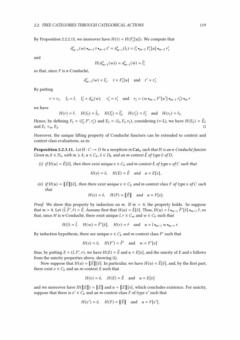
2.2. FREE CATEGORIES THROUGH CATEGORICAL ACTIONS 119

By Proposition 2.2.2.15, we moreover have � (C) = � (� ′1 [D]). We compute that

m+<−1(F) r<−2 C r<−2 C

′ = m+<−1(;1) = ; ′1 r<−2 �

′1 [D] r<−2 A

′1

and� (m+<−1(F)) = m+<−1(F) = ; ′1

so that, since � is =-Conduché,

m+<−1(F) = ; ′1, C = � ′1 [D] and C ′ = A ′1.

By putting

A = A1, ;2 = ;, ; ′2 = m−< (F), A ′2 = A

′1 and A2 = (F r

<−1 �′[D ′] r<−1 A

′2) r< A

we have� (A ) = A , � (;2) = ;2, � (; ′2) = ; ′2, � (A ′2) = A ′2 and � (A2) = A2.

Hence, by de�ning �2 = (; ′2, � ′, A ′2) and �2 = (;2, �2, A2), considering (≈-L), we have � (�2) = �2and �1 ≈< �2. �

Moreover, the unique lifting property of Conduché functors can be extended to context andcontext class evaluations, as in:

Proposition 2.2.3.11. Let� : � → � be a morphism in Cat= such that� is an =-Conduché functor.Given<,: ∈ N= with< ≤ : , D ∈ �: , E ∈ �: and an<-context � of type E of � ,

(i) if � (D) = � [E], then there exist unique E ∈ �: and<-context � of type E of � such that

� (E) = E, � (�) = � and D = � [E],

(ii) if � (D) = È�É[E], then there exist unique E ∈ �: and<-context class � of type E of � suchthat

� (E) = E, � (� ) = È�É and D = � [E].

Proof. We show this property by induction on <. If < = 0, the property holds. So supposethat< > 0. Let (; , � ′, A ) = �. Assume �rst that � (D) = � [E]. Thus, � (D) = ; r<−1 �

′[E] r<−1 A , sothat, since � is =-Conduché, there exist unique ;, A ∈ �< andF ∈ �: such that

� (;) = ; , � (F) = � ′[E], � (A ) = A and D = ; r<−1 F r<−1 A .

By induction hypothesis, there are unique E ∈ �: and<-context class � ′ such that

� (E) = E, � (� ′) = � ′ and F = � ′[E]

thus, by putting � = (;, � ′, A ), we have � (�) = � and D = � [E], and the unicity of � and E followsfrom the unicity properties above, showing (i).

Now suppose that � (D) = È�É[E]. In particular, we have � (D) = � [E], and, by the �rst part,there exist E ∈ �: and an<-context � such that

� (E) = E, � (�) = � and D = � [E]

and we moreover have � (È�É) = È�É and D = È�É[E], which concludes existence. For unicity,suppose that there is E ′ ∈ �: and an<-context class � of type E ′ such that

� (E ′) = E, � (� ) = È�É and D = � [E ′].

120 CHAPTER 2. THE WORD PROBLEM ON STRICT CATEGORIES

Let � ′ be an<-context such that � = È� ′É. So � ≈< � (� ′), and, by Proposition 2.2.3.10, thereexist an<-context � such that

� ≈< � and � (�) = � (� ′)

so we moreover have D = � [E]. Since D = � ′[E ′], by the unicity property of the �rst part, wehave E = E ′ and � = � ′, which implies È�É = � . Hence, (ii) holds. �

In order for monomorphisms to be preserved by the functor −[−]A, one needs the injectiveness oncells of such morphisms to extend to contexts and context classes. This is the case for Conduchémonomorphisms:

Proposition 2.2.3.12. Let � : � → � be a monomorphism in Cat= which is moreover =-Conduché.Given< ∈ N= and an<-type (D,D ′),� induces an injective function between<-contexts (resp.<-con-text classes) of type (D,D ′) of � and<-contexts (resp.<-context classes) of type (� (D), � (D ′)) of � .

Proof. We prove this property by induction on<. When< = 0, the property holds. So supposethat < > 0. Let �1 = (;1, � ′1, A1) and �2 = (;2, � ′2, A2) be two <-contexts of type (D,D ′) suchthat � (�1) = � (�2), i.e.,

� (;1) = � (;2), � (� ′1) = � (� ′2) and � (A1) = � (A2).

Thus, since � is a monomorphism, ;1 = ;2 and A1 = A2, and, by induction hypothesis, � ′1 = �′2.

Now let �1 and �2 be two <-context classes of type (D,D ′) of � such that � (�1) = � (�2).Let �1, �2 be <-contexts of type (D,D ′) such that �1 = È�1É and �2 = È�2É. Thus, we havethat � (�1) ≈< � (�2) and, by Proposition 2.2.3.10, there exists an<-context �1 such that

� (�1) = � (�2) and �1 ≈< �1

By the �rst part, �1 = �2, so that �1 ≈< �2, which implies �1 = �2. �

Finally, since we aim at showing that monomorphic Conduché functors are preserved by −[−]A,we prove that Conduché morphisms have a property of lifting of factorization of contexts andcontext classes analogous to the one on cells:

Proposition 2.2.3.13. Let� : � → � be a morphism in Cat= which is =-Conduché,< ∈ N= , (D,D ′)be an<-type of � , and � be an<-context of type (D,D ′). Suppose that either � is a monomorphismor (D,D ′) is an instantiable type. We then have:

(i) if � (�) = E r8 �′ for some 8 ∈ N<−1, E ∈ �8+1 and<-context � ′ of type (� (D), � (D ′)), then

there exist unique E ∈ �8+1 and<-context � ′ of type (D,D ′) such that

� (E) = E, � (� ′) = � ′ and � = E r8 �′,

(ii) if � (È�É) = E r8 � for some 8 ∈ N<−1, E ∈ �8+1 and<-context class � of type (� (D), � (D ′)),

then there exist unique E ∈ �8+1 and<-context � of type (D,D ′) such that

� (E) = E, � (� ) = � and È�É = E r8 � .

and similarly for compositions on the right of contexts and context classes by cells.

2.2. FREE CATEGORIES THROUGH CATEGORICAL ACTIONS 121

Proof. We show the property by induction on <. The property holds for < ≤ 1 so assumethat < > 1. Let � = (;, � , A ) be an <-context of type (D,D ′) such that � (�) = E r

8 �′ for

some 8 ∈ N<−1, E ∈ �8+1 and<-context � ′ = (; ′, � ′, A ′). If 8 + 1 =<, we then have

� (;) = E r<−1 ;

′, � (� ) = � ′ and � (A ) = A ′

thus, since � is =-Conduché, there are unique E ∈ �8+1 and ; ′ ∈ �< such that

� (E) = E, � (;) = ; ′ and ; = E r8 ;′

so that � = E r8 �′ with � ′ = (; ′, � , A ), and one easily check that the unicity property is veri�ed.

Otherwise, if 8 + 1 < <, we then have

� (;) = E r8 ;′, � (� ) = E r

8 �′, and � (A ) = E r

8 A′.

By induction hypothesis and since � is =-Conduché, there are unique E1, E2, E3 ∈ �8+1, ; ′, A ′ ∈ �<and (<−1)-context class � ′ such that

E = � (E1) E = � (E2) E = � (E3); ′ = � (; ′) � ′ = � (� ′) A ′ = � (A ′); = E1 r

8 ;′ � = E2 r

8 �′ A = E3 r

8 A′.

Moreover,E1 r

8 m+<−1(; ′) = m+<−1(;) = � [D] = E2 r

8 �′[D]

and� (m+<−1(; ′)) = m+<−1(; ′) = � ′[� (D)] = � (� ′[D])

so that, since � is =-Conduché,

E1 = E2 and m+<−1(; ′) = � ′[D]

Similarly,E2 = E3 and � ′[D ′] = m−<−1(A ′)

so that � = E1 r8 �′ where � ′ = (; ′, � ′, A ′), and the unicity of such a factorization is easily deduced

from the unicity of E1, ; ′, A ′ and � ′. Thus (i) holds.Now, suppose that � (È�É) = E r

8 � for some 8 ∈ N<−1, E ∈ �8+1 and (<−1)-context class � .Let � ′ be an<-context such that � = È� ′É. Then, � (�) ≈< E r

8 �′, so that, by Proposition 2.2.3.10,

there exists an<-context � of type (D,D ′) such that

� (�) = E r8 �′ and � ≈< �.

Then, by the �rst part, there exist E ∈ �8+1 and an<-context � ′ of type (D,D ′) such that

� (E) = E, � (� ′) = � ′ and � = E r8 �′.

Thus, by putting � = È� ′É, we have È�É = E r8 � . Suppose now that

� (E) = E, � (� ) = � and È�É = E r8 �

for some E ∈ �8+1 and <-context class � of type (D,D ′). If � is a monomorphism, then, byProposition 2.2.3.12, we have E = E and � = � . Otherwise, if (D,D ′) = (m−<−1(F), m+<−1(F)) forsomeF ∈ �< , then, by Proposition 2.2.2.13 and Proposition 2.2.2.15, we have

E r8 � [F] = � [F] = E r

8 � [F] and � (� [F]) = � [� (F)] = � (� [F])

so that, since � is =-Conduché, we have E = E and � [F] = � [F]. Moreover, since

� (� ) = � = � (� )

we have � = � by Proposition 2.2.3.11. Hence, (ii) holds. �

122 CHAPTER 2. THE WORD PROBLEM ON STRICT CATEGORIES

2.2.3.14 — Monomorphism preservation. Let = ∈ N. From the above properties on contextsand context classes, we �nally deduce a preservation property of monomorphisms of cellularextension by the free action functor:

Proposition 2.2.3.15. Let (�,ℎ) : (�,- ) → (�,. ) be a monomorphism in Cat+= , such that � is=-Conduché. The =-categorical action morphism � [ℎ]A is a monomorphism and an =-Conduchémorphism of CatA= .

Proof. Since (�,ℎ) is a monomorphism, both

� : � → � ∈ Cat= and ℎ : - → . ∈ Set

are monomorphisms. Since � [ℎ]A=+1((6, � )) = (ℎ(6), � (� )) for (6, � ) ∈ -A, we have that � [ℎ]Ais a monomorphism by Proposition 2.2.3.12. And it is =-Conduché as a consequence of Proposi-tion 2.2.3.13. �

2.2.4 Free (n+1)-categories on n-categorical actions

There is a forgetful functorU ′ : Cat=+1 → CatA=

which maps an (=+1)-category� to an =-categorical action (�≤=,�=+1) by forgetting the r= opera-

tion (where we consider the (=+1)-precategory structure of�). SinceU ′ is obviously derived froman essentially algebraic theory morphism, this functor has a left adjoint −[−]≈ : CatA= → Cat=+1by Theorem 1.1.2.7. In this section, given (�,�) ∈ CatA= , we show that the (=+1)-cells of � [�]≈can be described as sequences of composable elements of� that are adequately quotiented. More-over, we prove preservation properties of monomorphisms and Conduché functors for −[−]≈that are analogous to the ones proved in the previous section for −[−]A.

2.2.4.1 — Sequences. Let = ∈ N and (�,�) ∈ CatA= . We de�ne the set �★ of =-composablesequences (or simply, =-sequences) of (�,�) as the set of terms of the form

(D1, . . . , D: )s

for some : ∈ N and D1, . . . , D: ∈ � such that D1, . . . , D: are =-composable. When : = 0, byconvention, there is an empty sequence ( )sD for each D ∈ �= . Given E = (E1, . . . , E: )s ∈ �★, wesay that : is the length of E and we write |E | for : . Moreover, we de�ne a source m−= (E) and atarget m+= (E) for E by putting

m−= (E) = m−= (E1) and m+= (E) = m+= (E: )

where, by convention, if E = ( )sD for some D ∈ �= , then m−= (E) = m+= (E) = D. Thus, we obtain an=-cellular extension whose set of (=+1)-globes is �★ and whose underlying =-category is � . Wenow de�ne composition operations for the =-sequences. Given 8 ∈ N=−1, a cell D ∈ �8+1 and an=-sequence E = (E1, . . . , E; )s ∈ �★ such that D, E are 8-composable, we put

D r8 E = (D r

8 E1, . . . , D r8 E; )s

where, by convention, if E = ( )sE

for some E ∈ �= , then D r8 E = ( )s

D q8 E . Given =-composable=-sequences D = (D1, · · · , D: )s and E = (E1, · · · , E; )s in �★, we put

D r= E = (D1, . . . , D: , E1, . . . , E; )s.

2.2. FREE CATEGORIES THROUGH CATEGORICAL ACTIONS 123

; = G ~ I

5

5 ′

6⇓ D A = G ~ I

5

6

6′

⇓ E

; ′ = G ~ I5 ′

6

6′

⇓ E A ′ = G ~ I

5

5 ′

6′

⇓ D

Figure 2.2 – A con�guration of 2-cells ;, ; ′, A , A ′, D, E such that X(;, ; ′, A , A ′, D, E)

In order to obtain a strict (=+1)-category from � and �★, we need to quotient �★ so that theexchange condition (E) on precategories holds (c.f. Theorem 1.4.3.8). For this purpose, we de�nea relation

X ⊆ �6

such that, given ;, ; ′, A , A ′, D, E ∈ �, X(;, ; ′, A , A ′, D, E) holds when D, E are (=−1)-composable and thefollowing equalities hold in �

; = D r=−1 m

−= (E) A = m−= (D) r=−1 E

; ′ = m+= (D) r=−1 E A ′ = D r=−1 m

+= (E).

In Figure 2.2, we illustrate this condition in the case of a 1-categorical action. Given ;, ; ′, A , A ′ ∈ �,we write X(;, ; ′, A , A ′) when there exist D, E ∈ � such that we have X(;, ; ′, A , A ′, D, E). We de-�ne an equivalence relation ≈ on �★ as the re�exive symmetric transitive closure of ≈1, where,for ; = (;1, . . . , ;: )s and A = (A1, . . . , A: )s in �★, ; ≈1 A when there is 8 ∈ N∗

:−1 such that

X(;8 , ;8+1, A8 , A8+1) and ; 9 = A 9 for 9 ∈ N∗:\ {8, 8 + 1}.

We write �≈ for the quotient set �★/≈ of =-sequence classes and write

È−É : �★→ �≈

for the associated projection. We remark that, ifD, E ∈ �★ are such thatD ≈ E , then |D | = |E |. Thus,the length given for the members of �★ induces a length for the members of �≈.

Remark 2.2.4.2. The relation ≈−1 on�★, which is de�ned by D ≈−1 E when E ≈1 D for all D, E ∈ �★,admits a de�nition which is symmetrical to the one of ≈1. Moreover, ≈ can be equivalentlydescribed as the re�exive transitive closure of ≈1 ∪ ≈−1, so that, in the proofs, by symmetry ofthe de�nitions of ≈1 and ≈−1, we can often reduce a case analysis of D ≈ E to D ≈1 E .

Note that the operations mn= for n ∈ {−, +} on �★ are compatible with the relation ≈, so that theyare well-de�ned on �≈ as well. Thus, we obtain an =-cellular extension � [�]≈ by extending thestrict =-category � with �≈. The operations r

8 for 8 ∈ N=−1 and r= de�ned for �★ are compatible

with the relation ≈, so that they are well-de�ned on � [�]≈=+1 = �≈ as well. We add an identityoperation by putting id=+1D = È( )sDÉ for D ∈ �= . We then have:

Proposition 2.2.4.3. The operations id=+1 and r8 for 8 ∈ N= de�ned above equip � [�]≈ with a

structure of an (=+1)-precategory.

124 CHAPTER 2. THE WORD PROBLEM ON STRICT CATEGORIES

Proof. The axioms of (=+1)-precategories are then easily veri�ed from the de�nition of �★ andsince � [�]≈≤= = � is an =-precategory. �

More importantly, we have

Proposition 2.2.4.4. � [�]≈ has a structure of (=+1)-category.

Proof. We prove the criterion (E) that characterizes (=+1)-categories among (=+1)-precategoriesby Theorem 1.4.3.8. This criterion is already satis�ed by � , so that it is enough to verify it on(=+1)-cells. Given D ∈ � [�]≈=+1 (resp. E ∈ � [�]≈=+1), we write PL(D) (resp. PR(E)) when we have

(D r8−1 m

−8 (E)) r8 (m+8 (D) r8−1 E) = (m−8 (D) r8−1 E) r8 (D r

8−1 m+8 (E)) (2.6)

for all 8 ∈ N∗= and E ∈ � [�]≈8+1 (resp. D ∈ � [�]≈8+1) such that D, E are 8-composable. Note that (E) issatis�ed if and only if PL(D) and PR(D) for allD ∈ � [�]≈=+1. By symmetry, we only prove that PL(D)for all D ∈ � [�]≈=+1. We �rst show that, given D ∈ �= ,

PL(id=+1D ) holds. (2.7)

Indeed, for all 8 ∈ N∗=−1 and E ∈ �8+1 such that D, E are (8−1)-composable, we have

(id=+1Dr8−1 m

−8 (E)) r8 (m+8 (id=+1D ) r8−1 E)

= id=+1(D r8−1 m

−8 (E)) r8 (m+8 (D) r8−1 E)

= id=+1((D r8−1 m

−8 (E)) r8 (m+8 (D) r8−1 E))

= id=+1((m−8 (D) r8−1 E) r8 (D r8−1 m

+8 (E))) (by (E) in �)

= (m−8 (D) r8−1 E) r8 id=+1(D r8−1 m

+8 (E))

= (m−8 (D) r8−1 E) r8 (id=+1(D) r8−1 m+8 (E))

and, for all E ∈ �=+1 such that D, E are (=−1)-composable, we have

(id=+1Dr=−1 m

−= (E)) r= (m+= (id=+1D ) r=−1 E)

= id=+1(D r=−1 m

−= (E)) r= (m+= (id=+1D ) r=−1 E)

= D r=−1 (E)

= (m−= (id=+1D ) r=−1 (E)) r= id=+1(D r=−1 m

+= (E))

= (m−= (id=+1D ) r=−1 (E)) r= (id=+1Dr=−1 m

+= (E))

thus (2.7) holds. Now, we show that, given =-composable D1, D2 ∈ � [�]≈=+1,

PL(D1) and PL(D2) implies PL(D1 r= D2). (2.8)

Indeed, if PL(D1) and PL(D2) hold, then, for 8 ∈ N∗=−1 and E ∈ �8+1 such that D1, E is (8−1)-compo-sable, we have

[(D1 r= D2) r8−1 m

−8 (E)] r8 (m+8 (D1 r

= D2) r8−1 E)= [(D1 r

8−1 m−8 (E)) r= (D2 r

8−1 m−8 (E))] r8 (m+8 (D1 r

= D2) r8−1 E)= [(D1 r

8−1 m−8 (E)) r8 (m+8 (D1 r

= D2) r8−1 E)] r= [(D2 r8−1 m

−8 (E)) r8 (m+8 (D1 r

= D2) r8−1 E)]= [(D1 r

8−1 m−8 (E)) r8 (m+8 (D1) r8−1 E)] r= [(D2 r

8−1 m−8 (E)) r8 (m+8 (D2) r8−1 E)]

= [(m−8 (D1 r= D2) r8−1 E) r8 (D1 r

8−1 m+8 (E))] r= [(m−8 (D1 r

= D2) r8−1 E) r8 (D2 r8−1 m

+8 (E))]

(by PL(D1) and PL(D2))= (m−8 (D1 r

= D2) r8−1 E) r8 [(D1 r8−1 m

+8 (E)) r= (D2 r

8−1 m+8 (E))]

2.2. FREE CATEGORIES THROUGH CATEGORICAL ACTIONS 125

= (m−8 (D1 r= D2) r8−1 E) r8 [(D1 r

= D2) r8−1 m+8 (E)]

and, for E ∈ � [�]≈=+1 such that D1 and E are (=−1)-composable, we have

[(D1 r= D2) r=−1 m

−= (E)] r= (m+= (D1 r

= D2) r=−1 E)= [(D1 r

=−1 m−= (E)) r= (D2 r

=−1 m−= (E))] r= (m+= (D1 r

= D2) r=−1 E)= [(D1 r

=−1 m−= (E)) r= (D2 r

=−1 m−= (E))] r= (m+= (D2) r=−1 E)

= (D1 r=−1 m

−= (E)) r= [(D2 r

=−1 m−= (E)) r= (m+= (D2) r=−1 E)]

= (D1 r=−1 m

−= (E)) r= [(m−= (D2) r=−1 E) r= (D2 r

=−1 m+= (E))] (by PL(D2))

= [(D1 r=−1 m

−= (E)) r= (m+= (D1) r=−1 E)] r= (D2 r

=−1 m+= (E))

= [(m−= (D1) r=−1 E) r= (D1 r=−1 m

+= (E))] r= (D2 r

=−1 m+= (E)) (by PL(D1))

= (m−= (D1 r= D2) r=−1 E) r= [(D1 r

=−1 m+= (E)) r= (D2 r

=−1 m+= (E))]

= (m−= (D1 r= D2) r=−1 E) r= [(D1 r

= D2) r=−1 m+= (E)]

thus, (2.8) holds.

Hence, it is enough to show PL(D) for D = È(D ′)sÉ with D ′ ∈ �. Given 8 ∈ N∗=−1 and E ∈ �8+1 suchthat D, E are (8−1)-composable, the equality (2.6) holds since we have

(D ′ r8−1 m−8 (E)) r8 (m+8 (D ′) r8−1 E) = (m−8 (D ′) r8−1 E) r8 (D ′ r8 m+8+1(E))

by Axiom (A-iv). We show that (2.6) holds for E = È(E1, . . . , E: )sÉ ∈ � [�]≈=+1 such that D, E are(=−1)-composable, using an induction on : ∈ N. The case : = 0 corresponds to E = id=+1E forsome cell E ∈ �= , and, by a similar argument than the one used to show (2.7), we have that (2.6)holds. When : > 0, given E ′ = È(E2, . . . , E: )sÉ, we have

(D r=−1 m

−= (E)) r= (m+= (D) r=−1 E)

= (È(D ′)sÉ r=−1 m

−= (E1)) r= (m+= (D ′) r=−1 È(E1)sÉ) r= (m+= (D) r=−1 E

′) (since E = È(E1)sÉ r= E′)

= È(D ′ r=−1 m−= (E1), m+= (D ′) r=−1 E1)sÉ r

= (m+= (D) r=−1 E′)

= È(m−= (D ′) r=−1 E1, D′ r=−1 m

+= (E1))sÉ r

= (m+= (D) r=−1 E′) (by the de�nition of ≈)

= (m−= (D) r=−1 È(E1)sÉ) r= (D r=−1 m

+= (E1)) r= (m+= (D) r=−1 E

′)= (m−= (D) r=−1 È(E1)sÉ) r= (D r

=−1 m−= (E ′)) r= (m+= (D) r=−1 E

′)= (m−= (D) r=−1 È(E1)sÉ) r= (m−= (D) r=−1 E

′) r= (D r=−1 m

+= (E ′)) (by induction hypothesis)

= (m−= (D) r=−1 E) r= (D r=−1 m

+= (E)) (since E = È(E1)sÉ r

= E′)

thus (2.6) holds, which concludes the proof of PL(D). Hence, � [�]≈ is an (=+1)-precategorysatisfying (E), so it is an (=+1)-category by Theorem 1.4.3.8. �

Finally, we show that this construction is universal:

Proposition 2.2.4.5. � [�]≈ is the free (=+1)-category on the action (�,�) relatively to the forgetfulfunctorU ′.

Proof. Let � be an (=+1)-category and (�, 5 ) : (�,�) → (�≤=, �=+1) be a morphism of =-catego-rical action. We de�ne an (=+1)-functor � : � [�]≈ → � such that �≤= = � . We �rst de�ne �on �★ by putting

� (( )sD) = id=+1� (D) � ((E1, . . . , E: )s) = 5 (E1) r= · · · r= 5 (E: )

126 CHAPTER 2. THE WORD PROBLEM ON STRICT CATEGORIES

for D ∈ �= and =-composable E1, . . . , E: for some : ∈ N∗. Now, given D,D ′ ∈ � that are (=−1)-com-posable, we have [

5 (D) r=−1 � (m−= (D ′))] r=

[� (m+= (D)) r=−1 5 (D ′)

]=

[� (m−= (D)) r=−1 5 (D ′)

] r=

[5 (D) r=−1 � (m+= (D ′))

]by (E) on � . Thus, given D = (D1, . . . , D: )s and E = (E1, . . . , E; )s in �★ such that D ≈ E , wehave � (D) = � (E), so that � is well-de�ned on � [�]≈=+1 = �★/≈, and it is easily shown to be an(=+1)-functor. The operation (�, 5 ) ↦→ � de�ned above induces a function

\� : CatA= ((�,�), (�≤=, �=+1)) → Cat=+1(� [�]≈, �)

which is natural in � . Note that \� is injective, since 5 (D) = � (È(D)sÉ) for every D ∈ �. Itis moreover surjective since a (=+1)-functor � : � [�]≈ → � is uniquely determined by �≤=and (� (È(D)sÉ))D∈�. So � [�]≈ is the free (=+1)-category on the =-categorical action (�,�). �

In the following, for all =-categorical action (�,�), we write � [�]≈ for � [�]≈ as above. Theconstruction (�,�) ↦→ � [�]≈ uniquely extends to a functor

−[−]≈ : CatA= → Cat=+1

which is left adjoint toU ′. Given (�,ℎ) : (�,�) → (�, �) in Cat+= , the (=+1)-functor

� [ℎ]≈ : � [�]≈ → � [�]≈ ∈ Cat=+1

is de�ned by

� [ℎ]≈8 = �8 and � [ℎ]≈=+1(È(D1, . . . , D: )sÉ) = È(ℎ(D1), . . . , ℎ(D: ))sÉ

for 8 ∈ N= and (D1, . . . , D: )s ∈ �★.

2.2.4.6 — Monomorphism preservation. In this section, we complete the monomorphismpreservation result for −[−]A given in Proposition 2.2.3.15 with a similar one for −[−]≈. Likefor −[−]A, the functor −[−]≈ does not have to preserve monomorphisms in general because ofthe quotient with ≈ of the (=+1)-cells. However, as we will prove, it preserves monomorphismsthat are moreover Conduché. Indeed, the latters are well-behaved regarding the relation ≈ sincethey can “lift” it.

Let = ∈ N and (�, 5 ) : (�,�) → (�, �) be a morphism in CatA= . We write

5 ★ : �★→ �★

for the function which maps (D1, . . . , D: )s ∈ �★ to (5 (D1), . . . , 5 (D: ))s ∈ �★. Moreover, we write

5 ≈ : �≈ → �≈

for � [5 ]≈=+1. We �rst prove a lifting property for ≈:

Proposition 2.2.4.7. If (�, 5 ) is a monomorphism and =-Conduché, we then have

(i) for all ;, ; ′ ∈ � and A , A ′ ∈ � such that that X(5 (;), 5 (; ′), A , A ′), there exist unique A, A ′ ∈ �such that 5 (A ) = A , 5 (A ′) = A ′ and X(;, ; ′, A , A ′),

(ii) for all C ∈ �★ and C ′ ∈ �★ such that 5 ★(C) ≈ C ′, there is a unique C ′ ∈ �★ such that 5 ★(C ′) = C ′and C ≈ C ′.

2.2. FREE CATEGORIES THROUGH CATEGORICAL ACTIONS 127

Proof. Let ;, ; ′ ∈ � and A , A ′ ∈ � such that X(5 (;), 5 (; ′), A , A ′). So there exist D, E ∈ � satisfying

5 (;) = D r=−1 m

−= (E) A = m−= (D) r=−1 E

5 (; ′) = m+= (D) r=−1 E A ′ = D r=−1 m

+= (E).

Since (�, 5 ) is =-Conduché and a monomorphism, there exist D, E ∈ � such that

D = 5 (D) ; = D r=−1 m

−= (E)

E = 5 (E) ; ′ = m+= (D) r=−1 E .

By putting A = m−= (D) r=−1E and A ′ = D r=−1m

+=−1(E), we have 5 (A ) = A and 5 (A ′) = A ′ andX(;, ; ′, A , A ′).

The unicity of A, A ′ comes from the fact that 5 is a monomorphism. Thus (i) holds.Now let C ∈ �★ and C ′ ∈ �★ such that 5 ★(C) ≈ C ′. By Remark 2.2.4.2, it is enough handle the

case where 5 ★(C) ≈1 C ′. So suppose that 5 ★(C) ≈1 C ′. By (i), there is C ′ ∈ �★ such that 5 ★(C ′) = C ′and C ≈ C ′. The unicity of C ′ comes from the fact that 5 ★ is a monomorphism. Thus (ii) holds. �

We then deduce a monomorphism preservation result for −[−]≈:

Proposition 2.2.4.8. If (�, 5 ) is a monomorphism and =-Conduché, then the (=+1)-functor � [5 ]≈is a monomorphism.

Proof. Let D,D ′ ∈ �≈ such that 5 ≈(D) = 5 ≈(D ′), and C, C ′ ∈ �★ such that ÈCÉ = D and ÈC ′É = D ′.Note that 5 ★(C) ≈ 5 ★(C ′). By Proposition 2.2.4.7(ii), there exists C ∈ �★ such that

5 ★(C) = 5 ★(C ′) and C ≈ C .Since 5 is injective, 5 ★ is too. Thus, we have C = C ′, so that D = D ′. �

Moreover, Conduché functors are also preserved:

Proposition 2.2.4.9. If (�, 5 ) is a monomorphism and =-Conduché, then the (=+1)-functor � [5 ]≈is (=+1)-Conduché.

Proof. We use the characterization of (=+1)-Conduché functor given by Proposition 2.2.3.7. First,let D ∈ �≈ such that 5 ≈(D) = E r

8 D′ for some 8 ∈ N=−1, E ∈ �8+1 and D ′ ∈ �≈. Given C ∈ �★

and C ′ ∈ �★ such that ÈCÉ = D and ÈC ′É = D ′, we have

5 ★(C) ≈ E r8 C′

so that, by Proposition 2.2.4.7(ii), there exists C ∈ �★ such that

5 ★(C) = E r8 C′ and C ≈ C .

Since (�, 5 ) is monomorphic and =-Conduché, there exist E ∈ �8+1 and C ′ ∈ �★ such that

� (E) = E, 5 ★(C ′) = C ′ and C = E r8 C′.

Hence, putting D ′ = ÈC ′É, we have 5 ≈(D ′) = D ′ and D = E r8 D′. The unicity of E and D ′ is a

consequence of Proposition 2.2.4.8.Now, let D ∈ �≈ such that 5 ≈(D) = D1 r

= D2 for some D1, D2 ∈ �≈. Given C ∈ �★ and C1, C2 ∈ �★such that ÈCÉ = D, ÈC1É = D1 and ÈC2É = D2, we have

5 ★(C) ≈ C1 r= C2

so that, by Proposition 2.2.4.7(ii), there exists C ∈ �★ such that 5 ★(C) = C1 r= C2. Since r

= is de�nedas concatenation of lists on �★, there are C1, C2 ∈ �★ such that

5 ★(C1) = C1, 5 ★(C2) = C2 and C = C1 rC2.

By putting D1 = ÈC1É and D2 = ÈC2É, we have 5 ≈(D1) = D1, 5 ≈(D2) = D2 and D = D1 r= D2. The

unicity ofD1, D2 is a consequence of Proposition 2.2.4.8. We conclude using Proposition 2.2.3.7. �

128 CHAPTER 2. THE WORD PROBLEM ON STRICT CATEGORIES

2.2.5 Another description of free categories on cellular extensions

Let = ∈ N. We can sum up the content of the previous sections to give another description of thefunctor

−[−] : Cat+= → Cat=+1.

Indeed, since its right adjointV= : Cat=+1 → Cat+= is the composite of the right adjoints

U ′ : Cat=+1 → CatA= and U : CatA= → Cat=

we have, by Propositions 2.2.3.4, 2.2.4.5, 1.2.3.14 and 1.2.3.15, that there exists a canonical naturalisomorphism

Φ : −[−] ⇒ (−[−]≈) ◦ (−[−]A) (2.9)

and, writing [ and [ ′ for the units associated to the respective adjunctions

−[−] a V= and (−[−]≈) ◦ (−[−]A) a U ◦ U ′

we moreover have [ ′ = Φ ◦ [.

2.2.5.1 — Some properties of free extensions. This description allows us to prove severalproperties of the functor −[−]. First, we show that (=+1)-generators of an =-cellular extensionare injectively embedded in the associated free (=+1)-category:

Proposition 2.2.5.2. Given an =-cellular extension (�,- ), [ (�,- ) is a monomorphism.

Proof. Since [ ′ = Φ ◦ [, it is enough to prove that [ ′ is a monomorphism. By de�nition of thefunctors −[−]A and −[−]≈, [ ′(�,- ) : (�,- ) → � [-A]≈ is the identity on the 8-cells for 8 ∈ N= .Moreover, given 6 ∈ - , [ ′(�,- ) maps 6 to

[ ′(�,- ) (6) = È((6, �6))sÉ.

By the de�nition of ≈, the restriction of ≈ to sequences of length 1 is the identity relation. So,given generators 6,6′ ∈ - such that [ ′(�,- ) (6) = [

′(�,- ) (6

′), we have ((6, �6))s = ((6′, �6′))s, andin particular 6 = 6′. Thus, [ ′(�,- ) is a monomorphism and so is [ (�,- ) . �

Given an =-cellular extension (�,- ), the above proposition justi�es that, given 6 ∈ - , we di-rectly write 6 for [ (�,- ) . Our description of −[−] also induces a decomposition property for the(=+1)-cells of free extensions:

Proposition 2.2.5.3. Given an =-cellular extension (�,- ) and D ∈ � [- ]=+1, D can be written

�1 [61] ∗= · · · ∗= �: [6: ]

where : ∈ N, 68 ∈ - and �8 is an =-context class of type 68 for 8 ∈ N∗: . Moreover, : is unique for D.

Proof. By the isomorphism (2.9), it is su�cient to prove this property in (-A)≈. First note that,given 6 ∈ - and an =-context class � of type 6, by Lemma 2.2.3.3, we have the following equalitiesin (-A)≈:

È((6, � ))sÉ = � [È((6, �6))sÉ] = � [[ ′(�,- ) (6)].

By de�nition of (-A)≈, D ∈ (-A)≈ is of the form

D = È(D1, . . . , D: )sÉ

2.2. FREE CATEGORIES THROUGH CATEGORICAL ACTIONS 129

for some D8 ∈ -A for 8 ∈ N∗:. Moreover, each D8 is of the form

D8 = (68 , �8)

for some 68 ∈ - and =-context class �8 of type 68 . Thus, we have

D = È(D1)sÉ ∗= · · · ∗= È(D: )sÉ= �1 [[ ′(�,- ) (61)] ∗= · · · ∗= �: [[ ′(�,- ) (6: )]

which is the wanted form. Moreover, since the length of an =-sequence is preserved by ≈, : isunique for D. �

Finally, we can combine the monomorphism preservation results given for the functors −[−]Aand −[−]≈ to deduce a monomorphism preservation property for −[−]:

Proposition 2.2.5.4. Given a morphism (�, 5 ) : (�,- ) → (�,. ) ∈ Cat+= such that (�, 5 ) isa monomorphism and � is =-Conduché, we have that � [5 ] is a monomorphism and (=+1)-Conduché.

Proof. This is a consequence of Propositions 2.2.4.8, 2.2.4.9 and 2.2.3.15. �

2.2.5.5 — Monomorphisms of polygraphs. We conclude this section with a criterion for mono-morphisms of polygraphs which will be useful to prove that the word problem instance on apolygraph reduces to a word problem instance on a �nite subpolygraph. First, we adapt Proposi-tion 2.2.5.4 to polygraphs:

Proposition 2.2.5.6. Given = ∈ N∪{l} and a morphism � : P→ Q ∈ Pol= such that �8 : P8 → Q8is injective for 8 ∈ N= , then � ∗ : P∗ → Q∗ is a monomorphism and =-Conduché.

Proof. By a simple induction on = ∈ N, using Proposition 2.2.5.4. The property moreover holdsfor = = l since, given an l-functor � : � → � , � is a monomorphism (resp. l-Conduché) if andonly if �≤: is a monomorphism (resp. :-Conduché) for : ∈ N. �

We can now deduce the following criterion for monomorphisms of polygraphs, which alreadyappears in the work of Makkai:

Proposition 2.2.5.7 ([Mak05, Lemma 5.(9)(ii)]). Given = ∈ N ∪ {l} and a morphism � : P→ Qin Pol= , the following are equivalent:

(i) � is a monomorphism in Pol= ,

(ii) for 8 ∈ N= , �8 : P8 → Q8 is a monomorphism in Set,

(iii) � ∗ is a monomorphism in Cat= ,

(iv) for 8 ∈ N= , � ∗8 : P∗8 → Q∗8 is a monomorphism of Set.

Proof. We prove this property using an induction on = ∈ N. We can observe that the propertyholds for = = 0. So suppose that the property holds for some = ∈ N. We show that it holdsfor = + 1. So let (�, 5 ) : (P, - ) → (Q, . ) be a morphism of Pol=+1 with � : P → Q ∈ Pol=and 5 : - → . ∈ Set.

Proof that (i) implies (ii): Since (−)Pol≤= is a right adjoint, � is a monomorphism, so that, by induction

hypothesis, � ∗= is injective. Let 61, 62 ∈ - such that 5 (61) = 5 (62). Then, for n ∈ {−, +},

� ∗(dn= (61)) = � ∗(dn= (62)).

130 CHAPTER 2. THE WORD PROBLEM ON STRICT CATEGORIES

Since � ∗= is injective, we have dn= (61) = dn= (62). Let . = {∗} and (%,. ) be the (=+1)-polygraphsuch that

d−= (∗) = d−= (61) and d+= (∗) = d+= (61).

Denoting 5 8 : . → - for the functions such that 5 8 (∗) = 68 for 8 ∈ {1, 2}, 5 1 and 5 2 inducesmorphisms of polygraphs (idP, 5 1), (idP, 5 2) : (P, . ) → (P, - ) and we have

(�, 5 ) ◦ (idP, 5 1) = (�, 5 ) ◦ (idP, 5 2).

Since (�, 5 ) is a monomorphism, it implies 5 1 = 5 2, i.e., 61 = 62. Thus, 5 is an injective function.

Proof that (ii) implies (i): This is trivial.

Proof that (iii) implies (iv): For 8 ∈ N=+1, the functor (−)8 : Cat=+1 → Set is derived from amorphism of essentially algebraic theories. Thus, by Theorem 1.1.2.7, it is a right adjoint, andas such, it preserves monomorphisms. Hence, if � ∗ [5 ] is a monomorphism, then � ∗ [5 ]8 is amonomorphism for 8 ∈ N=+1.

Proof that (iv) implies (iii): A morphism � : � → � ∈ Cat=+1 is completely determined bythe �8 : �8 → �8 for 8 ∈ N=+1. Thus, if � ∗ [5 ]8 is a monomorphism for 8 ∈ N=+1, then � ∗ [5 ]is a monomorphism.

Proof that (ii) implies (iv): This is a consequence of Proposition 2.2.5.6.

Proof that (iv) implies (ii): By the induction hypothesis, �8 : P8 → Q8 is a monomorphism of setfor 8 ∈ N= . Moreover, we have the commutative diagram

- .

P∗ [- ]=+1 Q∗ [. ]=+1

5

[ (P∗,- ) [ (Q∗,. )

� ∗ [5 ]=+1

where [ (P∗,- ) is injective by Proposition 2.2.5.2, and � [5 ]=+1 is injective. Thus, 5 is injective.

For the extension to = = l , note that the functors (−)Pol≤:,l : Poll → Pol: for : ∈ N preserves

monomorphisms (since they are right adjoints by Proposition 1.3.3.12) and jointly re�ect them(since Poll is a limit cone on the categories Pol: ). Thus, � is a monomorphism in Poll if andonly if �≤: is a monomorphism in Pol: for : ∈ N. We then conclude using the same remark asthe one in the proof of Proposition 2.2.5.6. �

2.3 Computable free extensions

In order to consider decidability problems on strict categories, like the word problem, we must �rstclarify the notion of computability on these structures and, in particular, how to represent themcomputationally. In classical computable model theory [Har98; AK00], computable models arestructures whose sets are subsets ofN and whose operations are recursive functions between thosesubsets. However, this approach would be inadequate for our purposes since the constructionswe introduced for strict categories, like the functor −[−] : Cat+= → Cat=+1, do not produce strict(=+1)-categories whose sets of cells are subsets of N. Instead, we use encodings to witness thatthese sets can be represented as subsets of N and the structural operations (sources, targets,identities, compositions) as recursive functions between these subsets.

After recalling the de�nition of recursive functions, we introduce the setting of computabilitywith encodings that will then allow to de�ne computational descriptions of strict =-categories

2.3. COMPUTABLE FREE EXTENSIONS 131

(Section 2.3.1). Using this formalism, we give su�cient conditions for the free extension on acellular extension to be computable (Section 2.3.2). The constructive content of the proofs willultimately lead to a concrete computational implementation, as we will see in Section 2.4. Wethen consider the special case of polygraphs and give a more e�cient procedure to compute thefree strict category on a polygraph (Section 2.3.3).

2.3.1 Computability with encodings

In this section, we introduce the formalism of computability with encodings, after recallingsome elementary de�nitions and facts about recursive functions. The latter are essentially thefunctionsN→ Nwhose values can be computed by a program or an algorithm. We then introducecomputational descriptions for the higher categorical objects that we will manipulate (=-globularsets, =-categories, =-precategories and =-cellular extensions, etc.). These descriptions will consistin encodings and recursive functions that represent the structural operations of these objects bythe mean of the encodings. Using such descriptions, higher categorical objects can then be inputsand outputs of programs.

2.3.1.1 — Recursive functions. We recall the de�nition and several elementary properties ofrecursive functions. We refer the reader to existing monographs (like [Rog87]) for a more completepresentation.

Given two sets -,. , we write Part(-,. ) for the set of partial functions between - and . .A function 5 ∈ Part(-,. ) is total when it is de�ned on all - . There are several operations whichcan be de�ned between the partial functions in the sets Part(N: ,N).For : ∈ N and (;8)8∈N∗

:∈ N: , there is a composition operation

◦:,(;8 )8 : Part(N: ,N) ×∏8∈N∗

:

Part(N;8 ,N) → Part(N;1+···+;: ,N)

so that, given partial functions 6 ∈ Part(N: ,N) and 58 ∈ Part(N;8 ,N) for 8 ∈ N∗:, the partial

function ℎ = ◦:,(;8 )8 (6, (58)8) is such that, for G1 ∈ N;1, . . . , G: ∈ N;: , ℎ(G1, . . . , G: ) is de�ned if andonly if 58 (G8) is de�ned for 8 ∈ N∗

:and 6(51(G1), . . . , 5: (G: )) is de�ned, and in this case,

ℎ(G1, . . . , G: ) = 6(51(G1), . . . , 5: (G: )).

For : ∈ N, there is a recursion operation

d: : Part(N: ,N) × Part(N:+2,N) → Part(N:+1,N)

so that, given 5 ∈ Part(N: ,N) and 6 ∈ Part(N:+2,N), the partial function ℎ = d: (5 , 6) is suchthat, for all G1, . . . , G: ∈ N,

– ℎ(G1, . . . , G: , 0) is de�ned if and only if 5 (G1, . . . , G: ) is de�ned, and, in this case,

ℎ(G1, . . . , G: , 0) = 5 (G1, . . . , G: ),

– for = ∈ N, ℎ(G1, . . . , G: , = + 1) is de�ned if and only if both

ℎ(G1, . . . , G: , =) and 6(G1, . . . , G: , =, ℎ(G1, . . . , G=))

are de�ned and, in this case,

ℎ(G1, . . . , G: , = + 1) = 6(G1, . . . , G: , =, ℎ(G1, . . . , G=)).

132 CHAPTER 2. THE WORD PROBLEM ON STRICT CATEGORIES

For : ∈ N, there is a minimization operation

`: : Part(N:+1,N) → Part(N: ,N)

such that, given 5 ∈ Part(N:+1,N), the partial function 6 = `: (5 ) is so that, for all G1, . . . , G: ∈ N,

– if there exists a smallest number = ∈ N such that 5 (G1, . . . , G: , =) is non-zero or unde�ned,then

6(G1, . . . , G: ) = 5 (G1, . . . , G: , =)

(if 5 (G1, . . . , G: , =) is unde�ned, then 6(G1, . . . , G: ) is unde�ned),

– otherwise, 6(G1, . . . , G: ) is unde�ned.

We de�ne subsets Rec: ⊆ Part(N: ,N) for : ∈ N as the smallest family of subsets of Part(N: ,N)such that

– for all : ∈ N and 2 ∈ N, the total function (G1, . . . , G: ) ↦→ 2 is in Rec: ,

– for all : ∈ N∗ and 8 ∈ N∗:, the total function (G1, . . . , G: ) ↦→ G8 is in Rec: ,

– the total function G ↦→ G + 1 is in Rec1,

– given : ∈ N and (;8)8∈N∗:∈ N: , 6 ∈ Rec: , 58 ∈ Rec;8 for 8 ∈ N∗

:, the partial func-

tion ◦:,(;8 )8 (6, (58)8) is in Rec;1+···+;: ,

– given : ∈ N, 5 ∈ Rec: , 6 ∈ Rec:+2, the partial function d: (5 , 6) is in Rec:+1,

– given : ∈ N and 5 ∈ Rec:+1, the partial function `: (5 ) is in Rec: .

Given : ∈ N, a partial function 5 : N: → N is said to be recursive when 5 ∈ Rec: . It is well-known [Tur37] that 5 is recursive when one of the following equivalent conditions hold:

– there exists a Turing machingM such that 5 is de�ned on (G1, . . . , G: ) ∈ N: if and onlyifM halts on input (G1, . . . , G: ) and, in this case, 5 (G1, . . . , G: ) is the output ofM on thisinput;

– there exists a lambda-term C such that 5 (G1, . . . , G: ) is de�ned if and only if there existsG ∈ Nsuch that C [G1] . . . [G: ] is beta-equivalent to [G] and, in this case, 5 (G1, . . . , G: ) = G (where,for 8 ∈ N, [8] denotes Church-encoding of 8).

So, intuitively, recursive functions are the partial functions that can be computed by a program.In particular, functions like addition, multiplication, division are recursive. For every : ∈ N, thereexists a recursive function

h: : N:+1 → N

which is universal for recursive functions with : arguments, i.e., for every function 5 ∈ Rec: ,there exists 2 ∈ N, such that, for all G ∈ N: , h: (2, G) is de�ned if and only if 5 (G) is de�ned, and,in this case, h: (2, G) = 5 (G). We say that such 2 is a code for 5 . Moreover, the recursive function h:can be chosen such that there are recursive functions

◦:,(;8 )8 : N:+1 → N and d: : N2 → N and ¯: : N→ N

for : ∈ N and (;8)8 ∈ N: satisfying

2.3. COMPUTABLE FREE EXTENSIONS 133

– for 5 ∈ Rec: , 5 # ∈ N, 68 ∈ Rec;8 and 6#8 ∈ N for 8 ∈ N∗

:, if 5 # is a code for 5 and 6#

8 is a codefor 68 , then ◦:,(;8 )8 (5 #, (6#

8 )8) is a code for ◦:,(;8 )8 (5 , (68)8),

– for 5 ∈ Rec: , 5 # ∈ N, 6 ∈ Rec:+2, 6# ∈ N if 5 # is a code for 5 and 6# is a code for 6,then d: (5 #, 6#) is a code for d: (5 , 6),

– for 5 ∈ Rec:+1 and 5 # ∈ N, if 5 # is a code for 5 , then ¯(5 #) is a code for ` (5 ).

In the following, we suppose �xed a sequence of such universal function h: for : ∈ N. Finally, werecall that a subset ( ⊆ N: is said recursive or decidable when the characteristic function

1( : N: → {0, 1} ⊂ N

is recursive.

2.3.1.2 — Bijections on integers. In order to represent tuples of elements of N as one elementofN so that these tuples can be manipulated by recursive functions, one needs bijectionsN: → Nfor : ∈ N that have good properties regarding computability. We de�ne such bijections below.

Let \2 : N × N→ N be the function such that, for (21, 22) ∈ N2,

\2(21, 22) = 21 +(21 + 22) (21 + 22 + 1)

2.

We have that:

Proposition 2.3.1.3. \2 is bijective and both \2 and \−12 are recursive.

Proof. We de�ne a function \2 : N → N2 as follows: for every 2 ∈ N, we put \2(2) = (21, 22)where 21, 22 ∈ N are unique such that

(i) there is a unique : ∈ N which is the smallest integer such that 2 < : (:+1)2 ,

(ii) 21 = 2 − (:−1):2 ,

(iii) 22 =: (:+1)

2 − 2 − 1.

The function \2 is injective since, for 2, 21, 22, : as above, we have

: = 21 + 22 + 1 and 2 = 21 +(: − 1):

2.

Moreover, for (21, 22) ∈ N2 and : = 21 + 22 + 1, we have

(: − 1):2

≤ \2(21, 22) < 21 + 22 + 1 + (: − 1):2

=: (: + 1)

2

so that \2(\2(21, 22)) = (21, 22). Thus, \2 is a section of \2, so \2 is bijective and \−12 = \2. Moreover,

by their respective de�nitions, both \2 and \−12 are recursive. �

The following property will be useful for showing that an algorithm that takes tuples as inputsand involving recursion (i.e., the algorithm calls itself) is terminating:

Proposition 2.3.1.4. For all 21, 22 ∈ N, max(21, 22) ≤ \2(21, 22).

Proof. For all 21, 22 ∈ N, it is clear that 21 ≤ \2(21, 22) by de�nition of \2. Moreover, if 22 ∈ N∗,then we have 21 + 22 + 1 ≥ 2 so that 221 + 22 ≤ \2(21, 22), and the conclusion follows. �

134 CHAPTER 2. THE WORD PROBLEM ON STRICT CATEGORIES

We de�ne functions \= : N= → N for = ≥ 2. The function \2 was de�ned above and we put

\=+1 = \2 ◦ (1N × \=)for = ≥ 2. We easily verify by induction that

Proposition 2.3.1.5. For every = ∈ N with = ≥ 2, \= is bijective and both \= and \−1= are recursive.

Moreover, for all (21, . . . , 2=) ∈ N= , we have max(21, . . . , 2=) ≤ \= (21, . . . , 2=).

2.3.1.6 — Encodings. Given a set - , an encoding for - is the data of a relation E- ⊆ N ×- suchthat

(i) for all G ∈ - , there exists G# ∈ N such that G# E- G ,

(ii) for all G, G ′ ∈ - and 2 ∈ N such that 2 E- G and 2 E G ′, we have G = G ′.

The G# ∈ N such that G# E- G for some G ∈ - are called codes of G and the set

{2 ∈ N | there exists G ∈ - such that 2 E- G}is called the support of E- . The encoding - is said

– injective when, for all G ∈ - , there is a unique 2 ∈ N such that 2 E G ,

– decidable when the set{2 ∈ N | ∃G ∈ -, 2 E G}

is decidable,

– equality-decidable when the set

{(2, 2 ′) ∈ N × N | ∃G ∈ -, 2 E G and 2 ′ E G} (2.10)

is decidable.

We note that:

Proposition 2.3.1.7. Given a set - and an encoding E- of - , we have:

(i) if E- is equality-decidable, then it is decidable,

(ii) if E- is injective and decidable, then it is equality-decidable.

Proof. For (i), given 2 ∈ N, deciding whether “there exists G ∈ - such that 2 E- G” is equivalentto deciding whether “(G, G) belongs to the set (2.10)”. For (ii), given 21, 22 ∈ N, deciding whether“(21, 22) belongs to the set (2.10)” is equivalent to, since E- in injective, deciding whether “21 = 22and there exists G ∈ - such that 21 E- G”. �

Example 2.3.1.8. The set N admits a trivial encoding EN which is the identity relation. Thisencoding is injective, decidable and equality-decidable.Given two sets - and . equipped with respective encodings E- and E. , and a partial function

5 : - → .

we say that 5 is computable when there exists a recursive function 5 : N → N such that, forall G ∈ - and G# ∈ N with G# E- G , we have that if 5 (G) is de�ned, then 5 (G#) is de�ned, and, inthis case,

5 (G#) E. 5 (G).Such a function 5 is called a recursive model of 5 . Moreover, a code for 5 is a code of such afunction 5 . We easily verify that the sets equipped with encodings and the computable functionsbetween them form a category.

2.3. COMPUTABLE FREE EXTENSIONS 135

2.3.1.9 — Datatypes. As we will see in Section 2.3.2, the formalism of encodings allows statingin a precise sense how di�erent constructions on higher categories are computable. However,it is a rather low-level perspective which would likely di�er from the one taken by an actualimplementation of these constructions. Indeed, in common programming languages, a set isusually not encoded as a subset of N but as a subset of the inhabitants of some datatype. Thetwo approaches are essentially equivalent since a datatype t induces an encoding for the setof inhabitants of t (in a way we will not explain, since it is technical and depends on how theconsidered programming language is compiled). We shall mention this more concrete perspectiveon computability in parallel to the one with encodings by provinding hints on how to encode thedi�erent encountered sets with datatypes of OCaml. In the following, given a set ( , we say that (is encoded by a datatype t when ( is equipped with an inclusion from ( to the inhabitants of t .In this case, the restriction of the encoding on t induces an encoding on ( .

Remark 2.3.1.10. In the current implementation of OCaml, the int datatype can only encodenatural numbers up to 262 − 1. For simplicity, we shall assume in the following that int canrepresent all the natural numbers, so that N is encoded by int . This approximation should haveno practical consequences since the code for the word problem introduced in the next section isnot expected to be used on examples that require integers beyond 262 − 1.

Example 2.3.1.11. Under the assumption of Remark 2.3.1.10, the set of �nite increasing sequenceson N is naturally encoded by the datatype int list .

2.3.1.12 — Standard derivations of encodings. In order not to spend too much time de�ningencodings, we de�ne several derivations of encodings for several “data structures” that we consideras standard. These derived encodings will equip implicitly the sets associated with the “datastructures”: subset of a set, product of sets, coproduct of sets, set of �nite sequences over a set,set of �nite subsets of a set, dependent sum and functions with �nite domains.

Let- be a set and- ′ be a subset of- and E- be an encoding of- . We derive an encoding E- ′of - ′ by putting 2 E- ′ B when 2 E- B for 2 ∈ N and B ∈ - ′. We easily verify that:

Proposition 2.3.1.13. The following holds:

(i) if E- is injective, then E- ′ is injective,

(ii) if E- ′ is decidable and E- is equality-decidable, then E- ′ is equality-decidable.

Remark 2.3.1.14. If - is encoded by the datatype t , then - ′ is naturally encoded by t as well.

Let -1 and -2 be two sets together with encodings E-1 and E-2 . We derive an encoding E-1×-2

of -1 × -2 from E-1 and E-2 : for all 2 ∈ N and (G,~) ∈ -1 × -2, we put

2 E-1×-2 (G,~)

when, for 21, 22 ∈ N such that (21, 22) = \−12 (2), we have 21 E-1 G and 22 E-2 ~. We easily verify

the following property:

Proposition 2.3.1.15. If the encodings E-1 and E-2 are decidable (resp. equality-decidable, injec-tive), then E-1×-2 is decidable (resp. equality-decidable, injective).

Note that, given sets -1, . . . , -= for = ≥ 3 with encodings E-8 for 8 ∈ N∗= , we can derive similarlyan encoding E-1×···×-= for the product set -1 × · · · × -= , and this encoding satis�es a propertysimilar to Proposition 2.3.1.15.

136 CHAPTER 2. THE WORD PROBLEM ON STRICT CATEGORIES

Remark 2.3.1.16. If-1, . . . , -= are encoded by datatypes t1 , . . . , tn , then-1×· · ·×-= is naturallyencoded by the datatype type t = Tuple of t1 * ... * tn .

We also derive an encoding E-1t-2 of -1 t -2 from E-1 and E-2 : for 2 ∈ N, given G ∈ -1, we put

2 E-1t-2 ]-1 (G)

when 2 = \2(1, G#) for some G# ∈ N such that G# E-1 G ; given ~ ∈ -2, we put

2 E-1t-2 ]-2 (~)

when 2 = \2(2, ~#) for some ~# ∈ N such that ~# E-2 ~. We easily verify that

Proposition 2.3.1.17. If the encodings E-1 and E-2 are decidable (resp. equality-decidable, injec-tive), then E-1t-2 is decidable (resp. equality-decidable, injective).

Note that this de�nition adapts naturally to derive an encoding E-1t···t-= of a coproduct ofsets -1 t · · · t -= , and this encoding satis�es a property similar to Proposition 2.3.1.17.

Remark 2.3.1.18. If-1, . . . , -= are encoded by datatypes t1 , . . . , tn , then-1t· · ·t-= is naturallyencoded by the datatype type t = Inj1 of t1 | ... | Injn of tn .

We derive an encoding E-<l of the set -<l of �nite sequences of elements of - : for 2 ∈ N,given : ∈ N and (G1, . . . , G: ) ∈ -<l , we put

2 E-<l (G1, . . . , G: )

when 2 = \2(:, 2) with 2 = \: (21, . . . , 2: ) for some 2, 21, . . . , 2: ∈ N such that 28 E- G8 for 8 ∈ N∗:

(by convention, \2(0, 0) is the code of the empty sequence). We easily verify that E-<l is indeedan encoding and that:

Proposition 2.3.1.19. If the encoding E- is injective (resp. decidable, equality-decidable), then theencoding E-<l is injective (resp. decidable, equality-decidable).

Remark 2.3.1.20. If- is encoded by the datatype t , then-<l is naturally encoded by the datatypet list .

We derive an encoding EPf (- ) of the set Pf (- ) of �nite subsets of - : for 2 ∈ N, given : ∈ Nand G1, . . . , G: ∈ - with G8 ≠ G 9 for 8 ≠ 9 , we put

2 EPf (- ) {G1, . . . , G: }

when 2 = \2(:, 2) with 2 = \: (21, . . . , 2: ) for some 2, 21, . . . , 2: ∈ N satisfying

21 < · · · < 2:

and such that there exists a permutation f of N∗:

with 28 E- Gf (8) (by convention, \2(0, 0) is thecode for the empty set). The codes of the elements are required to be sorted in order to preservethe injectiveness. We verify:

Proposition 2.3.1.21. If the encoding E- is injective (resp. equality-decidable), then EPf (- ) isinjective (resp. equality-decidable).

2.3. COMPUTABLE FREE EXTENSIONS 137

Proof. The preservation of injectiveness is trivial. So suppose that E- is equality-decidable.Let 21, 22 ∈ N. We exhibit a procedure to decide whether there exists ( ∈ Pf (- ) such that

21 EPf (- ) ( and 22 EPf (- ) (

First, we verify that, for 8 ∈ {1, 2}, 28 EPf (- ) (8 for some (8 ∈ Pf (- ). We compute

(:8 , 28) = \−12 (28)

If :8 = 0, then 28 is a code if and only if 28 = 0 and, in this case, it is the code for the empty subset.Otherwise, if :8 > 0, we compute

(281, . . . , 28: ) = \−1:(28)

If the 281, . . . , 28:

are not sorted, then 28 is not the code of a �nite subset. So suppose that 281, . . . , 28:

are sorted. Then, 28 is the code of an element of Pf (- ) if and only if each 289 is the code of anelement of- for 9 ∈ N∗

:and, for 91, 92 ∈ N∗: with 91 ≠ 92, 2891 and 2892 encodes di�erent elements of- .

These two conditions can be veri�ed computationally since E- is supposed equality-decidable.So suppose that, for 8 ∈ {1, 2}, 28 EPf (- ) (

8 for some (8 ∈ Pf (- ). Then, (1 = (2 if and onlyif :1 = :2 and there exists a bijection f : N∗

:1→ N∗

:1such that 21

9 and 22f ( 9) encode the same

element of - for 9 ∈ N∗:1

. Once again, since E- is equality-decidable, this condition can beveri�ed computationally. Thus, EPf (- ) is equality-decidable. �

Remark 2.3.1.22. Our choice for the encoding of �nite subsets does not preserve decidability ingeneral. Indeed, to decide if 2 ∈ N is the code of a �nite subset of- , where 2 = \2(:, 2) with : ∈ N∗and 2 = \: (21, . . . , 2: ), we need to verify that the 2 9 encode di�erent elements of - , and we cannot do so computationally if we only know that E- is decidable. In fact, it can be easily shownthat if EPf (- ) is decidable, then E- is equality-decidable. However, other choices for EPf (- ) werepossible and, among them, ones that preserve decidability. But the one we proposed preservesinjectivity and that is our main concern for what is following.Remark 2.3.1.23. If - is encoded by the datatype t such that the set of inhabitants of t isequipped with a total order, then Pf (- ) is naturally encoded by the datatype t list . In practice,we can suppose all the datatypes we will consider to be equipped with total orders since OCamlcan automatically derive particular ones for us.Given moreover a �nite set ( and an encoding E( , we derive an encoding EF((,- ) of the setF ((, - )of functions ( → - : for 2 ∈ N and 5 : ( → - , we put

2 EF((,- ) 5

when 2 EPf ((×- ) {(B, 5 (B)) | B ∈ (}, i.e., 2 is the code of the graph of 5 , encoded as a �nite subsetof ( × - . From Proposition 2.3.1.15 and Proposition 2.3.1.21, we deduce that:

Proposition 2.3.1.24. If both E( and E- are injective (resp. equality-decidable), then EF((,- ) isinjective (resp. equality-decidable).

Remark 2.3.1.25. If ( and - are encoded by datatypes s and t respectively, then F ((, - ) isnaturally encoded by the datatype (s * t) list .Finally, given a function S : - → Set (i.e., for G ∈ - , S(G) is a set), and, for each G in - , anencoding ES(G) of S(G), we derive an encoding E∑

G S(G) of the dependent sum∑G ∈-S(G)

138 CHAPTER 2. THE WORD PROBLEM ON STRICT CATEGORIES

as follows: for all 2 ∈ N, G ∈ - and ~ ∈ S(G), we put

2 E∑G S(G) (G,~)

when 2 = \2(G#, ~#) for some G#, ~# ∈ N such that G# E- G and ~# ES(G) ~. We easily verify that:

Proposition 2.3.1.26. If E- is injective and ES(G) is injective for G ∈ - , then E∑G S(G) is injective.

Remark 2.3.1.27. If - is encoded by the datatype t , and, for G ∈ - , S(G) is encoded by thedatatype u , then

∑G ∈- S(G) is naturally encoded by the datatype t * u .

2.3.1.28 — Encodings for quotient sets. Under speci�c conditions, we can also derive encod-ings for quotients sets, and they will play an important role in the algorithm that solves theword problem. Given a set ( and a relation R on ( , R is right-�nite when, for all B ∈ ( , theset {B ′ ∈ ( | B R B ′} is �nite; given an encoding E( of ( , R is e�ectively right-�nite when thereis a computable function ' : ( → Pf (() such that, for all B, B ′ ∈ ( , B R B ′ if and only if B ′ ∈ '(B).Dually, there are notions of left-�nite and e�ectively left-�nite relations. The relationR is decidablewhen the characteristic function

1R : ( × ( → {0, 1} ⊂ N

is computable (where ( × ( is equipped with the encoding for product set given above and Nequipped with the trivial encoding on N).

Let - be a set and ∼ be an equivalence relation on - . Given G ∈ - , we write ÈGÉ ⊆ - for theequivalence class of G with regards to ∼. Let -/∼ be the set {ÈGÉ | G ∈ - }, i.e., the quotient of -by ∼. We say that ∼ has �nite classes when ÈGÉ is �nite for all G ∈ - . Equivalently, ∼ has �niteclasses if and only if ∼ is right-�nite (resp. left-�nite). Given an encoding E- of - , if ∼ has �niteclasses, we can derive an encoding E-/∼ of -/∼ by putting, for all 2 ∈ N and G ∈ - ,

2 E-/∼ ÈGÉ when 2 EPf (- ) ÈGÉ.

We then have:

Proposition 2.3.1.29. Suppose that ∼ has �nite classes. Then, the following hold:

(i) the function which maps an element B ∈ -/∼ to the �nite set of G ∈ - such that ÈGÉ = B iscomputable,

(ii) if E- is injective, then E-/∼ is injective,

(iii) if E- is equality-decidable and the relation ∼ is e�ectively right-�nite, then E-/∼ equality-decidable (and so, decidable) and the function È−É : - → -/∼ is computable.

Proof. Proof of (i): Since the code of B ∈ -/∼ is a code for the equivalence class of - de�ned by B ,the identity function N → N is a recursive model of the function which maps B ∈ -/∼ to theequivalence class de�ned by B .

Proof of (ii): This is a consequence of the fact that EPf (- ) is injective when E- is by Proposi-tion 2.3.1.21.

Proof of (iii): Suppose that E- is equality-decidable and ∼ is e�ectively right-�nite. Then, byProposition 2.3.1.21, EPf (- ) is equality-decidable. Since ∼ is e�ectively right-�nite, the func-tion ' : - → Pf (- ) which maps G ∈ - to its equivalence class is computable, relatively to theencodings E- and EPf (- ) . So, let 21, 22 ∈ N. We give a procedure to decide if there is G ∈ -

2.3. COMPUTABLE FREE EXTENSIONS 139

such that 21 E-/∼ ÈGÉ and 22 E-/∼ ÈGÉ. Let (:, 21) = \−12 (21). If : = 0, then 21 is not a code

for an element of -/∼. So suppose that : > 0. We compute (211, . . . , 2

1:) = \−1

:(2). Since E-

is equality-decidable, we verify that 211 is the code for an element G ∈ - . If it is not the case,

then 21 is not a code for an element of -/∼. Otherwise, since ' is computable, we compute theequivalence class - ′ = '(G) of G . Then, by our de�nition of E-/∼, 21 and 22 encode the sameelement of-/∼ if and only if 21 EPf (- ) -

′ and 22 EPf (- ) -′, which can be decided since EPf (- ) is

equality-decidable by Proposition 2.3.1.21. Moreover, the function È−É : - → -/∼ is computablesince, for G ∈ - , a code of ÈGÉ is given by a code of '(G), which can be computed since ' iscomputable. �

Remark 2.3.1.30. If- is encoded by a datatype t and ∼ has �nite classes, then, by Remark 2.3.1.23,the set -/∼ is naturally encoded by the datatype t list .

We often do not have a direct description of the equivalence relation ∼, and instead have arelation ∼1 such that ∼ is the re�exive transitive closure of ∼1. In such a situation, we will usethe following property:

Proposition 2.3.1.31. Given a set ( with an encoding E( , a relation ∼1 on ( and an equivalencerelation ∼ on ( , such that E( is equality-decidable, ∼1 is e�ectively right-�nite and ∼ has �niteclasses on ( and is the re�exive transitive closure of ∼1, we have that ∼ is e�ectively right-�nite, E(/∼is equality-decidable and the function È−É : ( → (/∼ is computable.

Proof. Let ' : ( → Pf (() be the computable function such that, for all B, B ′ ∈ ( , B ∼1 B ′ if and onlyif B ′ ∈ '(B). Using ', we can compute the equivalence class of B ∈ ( by the following procedure,which is essentially a breadth-�rst search algorithm:

function ComputeClass(B)# ← {B}� ← ∅while # ≠ ∅ do

choose B ′ ∈ ## ← # \{B ′}if B ′ ∉ � then

� ← � ∪ {B ′}# ← # ∪ '(B ′)

end if

end while

return �

end function

Note that this procedure terminates on any B ∈ ( since � contains elements B ′ such that B ∼ B ′and ∼ has �nite classes, and, at each loop turn, either one element is removed from # or oneelement is added to � , so that it gives a function ComputeClass : ( → Pf ((). Moreover, thisfunction is computable since E( is equality-decidable. So ∼ is e�ectively right-�nite and Proposi-tion 2.3.1.29(iii) applies. �

2.3.1.32 — Encodings for recursive functions. For : ∈ N, by our choice of the universal func-tions h: , there are encodings ERec: of Rec: de�ned as follows: for all 5 ∈ Rec: and 5 # ∈ N, 5 # E 5if and only if

h: (5 #,−) = 5 (−).

By standard undecidability theorems on recursive functions, like Rice’s theorem, these encodingsare neither injective, nor equality-decidable. Decidability depends on the choice for h: . However,

140 CHAPTER 2. THE WORD PROBLEM ON STRICT CATEGORIES

the restrictions of the functions ◦:,(;8 )8 , d: and `: for : ∈ N and (;8)8 ∈ N: to recursive functionsare computable: recursive models are given by the function ◦:,(;8 )8 , d: and ¯: . This enables towrite algorithms that take as inputs computable functions and outputs computable functions.

Remark 2.3.1.33. In particular, and this will be important in the following, any constructive proofof a property that concludes that some function 5 is computable under some hypothesis leads toan algorithm which computes a code for 5 from a code for this hypothesis.

2.3.1.34 — Computational categorical descriptions. In this paragraph, we introduce computa-tional descriptions, or codes, for several higher categorical structures: =-globular set, =-categories,=-precategories and =-cellular extensions. Such descriptions are the data of codes of recursivefunctions that are recursive models for the di�erent structural operations that appear in the de�-nition of each structure. These descriptions will enable such higher categorical structures to beinputs and outputs of computable functions.

Let = ∈ N. Given an =-globular set � , an encoding E� of � is the data of encodings E8 ofthe sets �8 for 8 ∈ N=; it is injective (resp. decidable, equality-decidable) when E8 is injective(resp. decidable, equality-decidable) for 8 ∈ N= . Given such an encoding E� , the =-globular set �is computable when the functions m−8 , m

+8 : �8+1 → �8 are computable for 8 ∈ N=−1. A recursive

model of � is the data of recursive models m−8 , m+8 : N→ N of m−8 and m+8 respectively for 8 ∈ N=−1.

A code for� is the data of m−,#8, m+,#8∈ N for 8 ∈ N=−1 such that m−,#

8and m+,#

8are codes for m−8 and m+8

respectively.Given a strict=-category� and an encoding E� of� (seen as an=-globular set),� is computable

when the underlying =-globular set of � is computable and

– for : ∈ N=−1, the function id:+1 : �: → �:+1 is encodable,

– for 8, : ∈ N= with 8 < : , the functions ∗8,: : �: ×8 �: → �: (seen as a partial function oftype �: ×�: → �: ) is computable.

A recursive model of � is the data of a recursive model of the underlying =-globular set of �together with

– for : ∈ N=−1, a recursive model id:+1 : N→ N of id:+1,

– for 8, : ∈ N with 8 < : , a recursive model ∗8,: : N→ N of ∗8,: .

A code of � is the data of a code of the underlying =-globular set of � , together with codes id:+1,#

of id:+1 for : ∈ N=−1, and codes ∗#8,:

of ∗8,: for 8, : ∈ N= with 8 < : . Using \< for the correct valueof< ∈ N, a code of � can be represented as one element of N.

Remark 2.3.1.35. If�0 t · · · t�= is encoded by a datatype cell , then a recursive model of� canbe represented by OCaml functions

– csrc, ctgt : int -> cell -> cell ,

– identity : int -> cell -> cell ,

– comp : int -> int -> cell -> cell -> cell .

Given an =-precategory � and an encoding E� of � (seen as an =-globular set), � is computablewhen the underlying =-globular set of � is computable and

– for : ∈ N=−1, the function id:+1 : �: → �:+1 is computable,

2.3. COMPUTABLE FREE EXTENSIONS 141

– for 8, :, ; ∈ N= with 8 = min(:, ;) −1, the function r:,; : �: ×8 �; → �max(:,;) (seen as a partial

function of type �: ×�; → �max(:,;) ) is computable.

We de�ne the notions of recursive model and code of � as expected.Remark 2.3.1.36. If�0 t · · · t�= is encoded by a datatype cell , then a recursive model of� canbe represented by means of OCaml functions in a way analogous to Remark 2.3.1.35.We verify that the de�nition of “computable” is coherent between =-categories and =-precate-gories:

Proposition 2.3.1.37. Given an =-category � and an encoding E� of � , the =-category � is com-putable if and only if the =-precategory � is computable.

Proof. By Remark 2.3.1.33, the constructive content of the proof of Proposition 1.4.3.2 inducesan algorithm which computes a code of the =-precategory � from a code of the =-category � .Conversely, the proof of Proposition 1.4.3.4 induces an algorithm which computes a code of the=-category � from a code of the =-precategory � . Thus, the proposition holds. �

Given an =-cellular extension (�,- ) ∈ Cat+= , an encoding E (�,- ) of (�,- ) is the data of anencoding E�= (E8)8∈N= of � (seen as an =-globular set) together with an encoding E- of - . Itis injective (resp. decidable, equality-decidable) when both E� and E- are. Given such an encod-ing E (�,- ) , the =-cellular extension (�,- ) is computable when the =-category � is computableand the functions d−= , d

+= : - → �= are computable. A recursive model of (�,- ) is the data of a

recursive model of the =-category � together with recursive models d−= , d+= of the functions d−=

and d+= respectively. A code of (�,- ) is the data of a code of the =-category � together withcodes d−,#= , d+,#= of d−= and d+= respectively.

Finally, given an =-categorical action (�,�) and an encoding E (�,�) of (�,�) (seen as an=-cellular extension), (�,�) is computable when the underlying =-cellular extension of (�,�) iscomputable and, for 8 ∈ N=−1, the functions

r8+1,=+1 : �8+1 ×8 �→ � and r

=+1,8+1 : � ×8 �8+1 → �

are computable (as partial functions on domains �8+1 � and � �8+1 respectively). The notionsof recursive model and of code of (�,�) are de�ned as expected.

2.3.2 Computable free cellular extensions

In this section, we give conditions for which we can compute codes for free (=+1)-categories fromcodes of =-cellular extensions. Using the decomposition of the functor −[−] : Cat+= → Cat=+1given in Section 2.2, this amounts to give conditions for which we can compute codes for theimages of the functors

−[−]A : Cat+= → CatA= and − [−]≈ : CatA= → Cat=+1

The main obstacle for computability of the images of these functors are respectively the quotientsof <-contexts by the equivalence relations ≈< , and the quotient of sequences using the equiv-alence relations ≈. Indeed, in each case, we must ensure that we can compute the equivalenceclasses associated with each equivalence relations. Our plan is to use Proposition 2.3.1.31 on ≈1

<

and ≈1, so that we need to �nd conditions for which ≈1< and ≈1 have �nite classes and are ef-

fectively right-�nite. The conditions we propose are some �nite factorization properties on cellsof =-cellular extension and =-categorical actions, so that there are a �nite number of possibleinstances of the axioms de�ning ≈1

< and ≈1 for each equivalence classes.

142 CHAPTER 2. THE WORD PROBLEM ON STRICT CATEGORIES

2.3.2.1 — Finitely factorizable precategories. Let = ∈ N. Given an =-precategory � , � is�nitely factorizable when we have that

– for all 8 ∈ N=−2 and D ∈ �8+2, there is a �nite number of pairs

(D1, D2) ∈ �8+2 ×8 �8+1 t�8+1 ×8 �8+2 (2.11)

such that D = D1 r8 D2,

– for all 8 ∈ N=−1 and D ∈ �8+1, there is a �nite number of pairs

(D1, D2) ∈ �8+1 ×8 �8+1 (2.12)

such that D = D1 r8 D2.

When � is equipped with an encoding E� , we say that � is e�ectively factorizable when it is�nitely factorizable and moreover

– for 8 ∈ N=−2, there is a computable function

�8+2 → Pf (�8+2 ×�8+1 t�8+1 ×�8+2)

which takes as input D ∈ �8+2 and outputs the �nite set of pairs (D1, D2) as in (2.11) suchthat D = D1 r

8 D2,

– for 8 ∈ N=−1, there is a computable function

�8+1 → Pf (�8+1 ×�8+1)

which takes as input D ∈ �8+1 and outputs the �nite set of pairs (D1, D2) as in (2.12) suchthat D = D1 r

8 D2.

Remark 2.3.2.2. If �0 t · · · t �= is encoded by a datatype cell , then the above computablefunctions can be represented by OCaml functions

– cfact_het_l : int -> cell -> (cell * cell) list ,

– cfact_het_r : int -> cell -> (cell * cell) list ,

– cfact_hom : int -> cell -> (cell * cell) list ,

where, for 8 ∈ N=−2, we identify �nite subsets of �8+2 × �8+1 t �8+1 × �8+2 with pairs of �nitesubsets of �8+2 ×�8+1 and �8+1 ×�8+2.

Since strict categories are canonically precategories by Theorem 1.4.3.8, the notions of �nitefactorizability and e�ective factorizability for precategories directly translate to strict categories.We then verify that the �nite factorizability property on cells induces a �nite factorizabilityproperty with regard to contexts and context classes:

Proposition 2.3.2.3. Given a �nitely factorizable� ∈ Cat= and< ∈ N∗= , for allD, E ∈ �< , there is a�nite number of<-contexts � (resp.<-context class � ) of type (m−<−1(D), m+<−1(D)) such that � [D] = E(resp. � [D] = E).

2.3. COMPUTABLE FREE EXTENSIONS 143

Proof. We prove this property by an induction on<. If< = 0, then the property is trivial. So sup-pose that< ≥ 1. Let D, E ∈ �< and consider the set ( of<-contexts � of type (m−<−1(D), m+<−1(D))such that � [D] = E . By de�nition, the elements of ( are the triples (;, � ′, A ) where ;, A ∈ �< and � ′is an (<−1)-context class of type (m−<−2(D), m+<−2(D)) such that

m+<−1(;) = � ′[m−<−1(D)], � ′[m+<−1(D)] = A and ; r<−1 �′[D] r<−1 A = E .

By the �nite factorization property, the number of triples (;, � ′[D], A ) obtained by iterating on theelements (;, � ′, A ) of ( is �nite. In particular, by Proposition 2.2.2.2, the number of (<−1)-cells

� ′[m−<−1(D)] = m−<−1(� ′[D])

for (;, � ′, A ) ∈ ( is �nite. Thus, by induction hypothesis, there is a �nite number of possible(<−1)-context classes � ′ in the triples (;, � ′, A ) of ( . Hence, ( is �nite. Since<-context classes arequotient of<-contexts, we deduce moreover that there is a �nite number of<-context classes �such that � [D] = E . �

2.3.2.4 — Finitely factorizable actions. Let = ∈ N. An =-categorical action (�,�) is �nitelyfactorizable when the underlying strict =-category � is �nitely factorizable and, in the casewhere = > 0, for every D ∈ �, there is a �nite number of pairs

(D1, D2) ∈ � ×=−1 �= t�= ×=−1 � (2.13)

such that D = D1 r=−1 D2. When (�,�) is equipped with an encoding E (�,�) , we say that (�,�) is

e�ectively factorizable when it is �nitely factorizable, and moreover � is e�ectively factorizable,and there exists a computable function

�→ Pf (� ×=−1 �= t�= ×=−1 �)

which, on input D ∈ �, outputs the �nite set of pairs (D1, D2) as in (2.13) such that D = D1 r=−1 D2.

Remark 2.3.2.5. If �0 t · · · t�= and � are encoded by datatypes cell and cell_top respec-tively, then the computable functions which witness that (�,�) is e�ectively factorizable can berepresented by means of OCaml functions in a way analogous to Remark 2.3.2.2.

2.3.2.6 — Contexts and computability. Let = ∈ N and � be an =-category equipped withan encoding E� which is injective and decidable and such that � is computable and e�ectivelyfactorizable. We prove below several computational properties on the contexts of � . First, thecontexts and contexts classes of � on instantiable types admit encodings derived from E� forwhich several elementary operations on contexts and contexts classes are derivable:

Proposition 2.3.2.7. For< ∈ N= , D ∈ �< and D ′ = (m−<−1(D), m+<−1(D)), the following holds:

(i) there are canonical injective encodings of the<-contexts and<-context classes of type D ′,

(ii) the equivalence classes of<-contexts of type D ′ under ≈< are �nite, and the function mappingan<-context class � of type D ′ to the �nite set of<-context � of type D ′ such that È�É = � iscomputable,

(iii) for 8 ∈ N<−1 and n ∈ {−, +}, the function which takes as input an <-context � (resp. an<-context class � ) of type D ′ and outputs mn8 (�) (resp. mn8 (� )) is computable,

(iv) for : ∈ {<, . . . , =}, the function which takes as input an<-context � (resp.<-context class � )of type D ′ and a cell E ∈ �: of <-type D ′ and outputs the cell � [E] (resp. � [E]) of �: iscomputable.

144 CHAPTER 2. THE WORD PROBLEM ON STRICT CATEGORIES

Proof. We show this property by induction on <. There is a unique 0-context (resp. 0-contextclass) of type D ′ which can be encoded by 0 ∈ N. Thus, the case< = 0 holds. So suppose< ≥ 1.

Proof of (i): We de�ne an encoding for<-contexts (;, � , A ) of type D ′ using the standard derivationof encodings for triples based on the encodings of �< and of (<−1)-context classes obtained byinduction hypothesis, so that we get an encoding which is injective. By Proposition 2.3.2.3, therestriction of the equivalence relation ≈< to<-contexts of type D ′ has �nite classes, so that weobtain an encoding of<-context classes of type D ′ using the standard derivation of encodings forquotient sets based on the encoding of (<−1)-contexts of type D ′, and this encoding is injectiveby Proposition 2.3.1.29(ii).

Proof of (ii): Note that, given two <-contexts �1, �2 of type D ′ such that �1 ≈< �2, we havethat �1 [D] = �2 [D]. Thus, by Proposition 2.3.2.3, the equivalence classes of<-contexts of type D ′under ≈< are �nite. By our choice of encodings in (i), the identity function is a recursive modelof the function which maps an (<−1)-context class � of type D ′ to the �nite list of codes of(<−1)-contexts � of type D ′ such that È�É = � , so that the latter function is computable.

Proof of (iii): Let 8 ∈ N<−1. For all <-context � = (;, � ′, A ), m−8 (�) is de�ned as m−8 (;). Since theoperations m−8 on<-cells of� is computable by hypothesis on� and E� , the function which mapsan <-context � of type D ′ to m−8 (�) is computable. For all <-context class � , m−8 (� ) is de�nedas m−8 (�) where � is an <-context such that È�É = � . Since, by (ii), we have a computablefunction which maps an<-context class � of type D ′ to the (non-empty) set of<-context � suchthat � = È�É, the function which maps an<-context � of type D ′ to m−8 (� ) is computable. Andsimilarly for the target operations.

Proof of (iv): Let : ∈ {<, . . . , =}. Recall that, for an<-context � = (;, � , A ) of type D ′ and E ∈ �:+1of<-type D ′, � [E] is de�ned by

� [E] = ; r<−1 � [E] r<−1 A

so that, by the induction hypothesis, and since � is supposed computable, the function whichtakes as inputs � and E as above, and outputs the cell � [E], is computable. For context classes,recall that, for an<-context class � of type D ′ and E ∈ �:+1 of<-type D ′, � [E] is de�ned by

� [E] = � [E]

where � is some<-context such that È�É = � . Hence, by (ii), the function which takes as inputs �and E as above, and outputs the cell � [E], is computable. �

Remark 2.3.2.8. Note that the proof of Proposition 2.3.2.7 only used the fact that � was �nitelyfactorizable and not e�ectively factorizable.

Remark 2.3.2.9. If �0 t · · · t �= is encoded by a datatype cell , then, by the proof of Proposi-tion 2.3.2.7(i),<-contexts and<-contexts classes on some type D ′ ∈ �= are naturally encoded bythe datatypes

type ctxt =| CtxtZ (* constructor for the 0-context *)| CtxtS of cell * ctxtcl * cell (* constructor for the (m+1)-contexts *)and ctxtcl = ctxt list

as a consequence of Remarks 2.3.1.16 and 2.3.1.30.

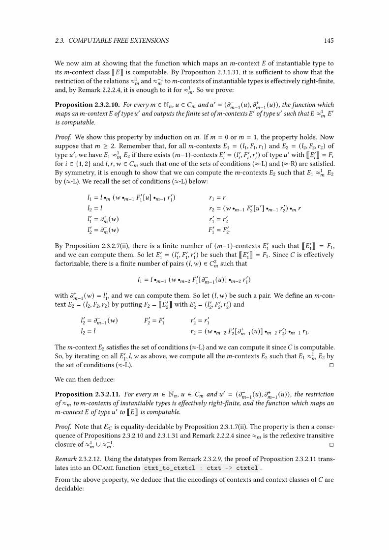
2.3. COMPUTABLE FREE EXTENSIONS 145

We now aim at showing that the function which maps an <-context � of instantiable type toits <-context class È�É is computable. By Proposition 2.3.1.31, it is su�cient to show that therestriction of the relations ≈1

< and ≈−1< to<-contexts of instantiable types is e�ectively right-�nite,

and, by Remark 2.2.2.4, it is enough to it for ≈1< . So we prove:

Proposition 2.3.2.10. For every< ∈ N= , D ∈ �< and D ′ = (m−<−1(D), m+<−1(D)), the function whichmaps an<-context � of typeD ′ and outputs the �nite set of<-contexts � ′ of typeD ′ such that � ≈1

< � ′

is computable.

Proof. We show this property by induction on <. If < = 0 or < = 1, the property holds. Nowsuppose that < ≥ 2. Remember that, for all <-contexts �1 = (;1, �1, A1) and �2 = (;2, �2, A2) oftype D ′, we have �1 ≈1

< �2 if there exists (<−1)-contexts � ′8 = (; ′8 , � ′8 , A ′8 ) of type D ′ with È� ′8É = �8for 8 ∈ {1, 2} and ;, A ,F ∈ �< such that one of the sets of conditions (≈-L) and (≈-R) are satis�ed.By symmetry, it is enough to show that we can compute the<-contexts �2 such that �1 ≈1

< �2by (≈-L). We recall the set of conditions (≈-L) below:

;1 = ; r< (F r<−1 �

′1 [D] r<−1 A

′1) A1 = A

;2 = ; A2 = (F r<−1 �

′2 [D ′] r<−1 A

′2) r< A

; ′1 = m+< (F) A ′1 = A

′2

; ′2 = m−< (F) � ′1 = �

′2.

By Proposition 2.3.2.7(ii), there is a �nite number of (<−1)-contexts � ′1 such that È� ′1É = �1,and we can compute them. So let � ′1 = (; ′1, � ′1, A ′1) be such that È� ′1É = �1. Since � is e�ectivelyfactorizable, there is a �nite number of pairs (;,F) ∈ �2

< such that

;1 = ; r<−1 (F r<−2 �

′1 [m−<−1(D)] r<−2 A

′1)

with m+<−1(F) = ; ′1, and we can compute them. So let (;,F) be such a pair. We de�ne an<-con-text �2 = (;2, �2, A2) by putting �2 = È� ′2É with � ′2 = (; ′2, � ′2, A ′2) and

; ′2 = m−<−1(F) � ′2 = �

′1 A ′2 = A

′1

;2 = ; A2 = (F r<−2 �

′2 [m+<−1(D)] r<−2 A

′2) r<−1 A1.

The<-context �2 satis�es the set of conditions (≈-L) and we can compute it since� is computable.So, by iterating on all � ′1, ;,F as above, we compute all the<-contexts �2 such that �1 ≈1

< �2 bythe set of conditions (≈-L). �

We can then deduce:

Proposition 2.3.2.11. For every < ∈ N= , D ∈ �< and D ′ = (m−<−1(D), m+<−1(D)), the restrictionof ≈< to<-contexts of instantiable types is e�ectively right-�nite, and the function which maps an<-context � of type D ′ to È�É is computable.

Proof. Note that E� is equality-decidable by Proposition 2.3.1.7(ii). The property is then a conse-quence of Propositions 2.3.2.10 and 2.3.1.31 and Remark 2.2.2.4 since ≈< is the re�exive transitiveclosure of ≈1

< ∪ ≈−1< . �

Remark 2.3.2.12. Using the datatypes from Remark 2.3.2.9, the proof of Proposition 2.3.2.11 trans-lates into an OCaml function ctxt_to_ctxtcl : ctxt -> ctxtcl .

From the above property, we deduce that the encodings of contexts and context classes of � aredecidable:

146 CHAPTER 2. THE WORD PROBLEM ON STRICT CATEGORIES

Proposition 2.3.2.13. Given< ∈ N= , D ∈ �< and D ′ = (m−<−1(D), m+<−1(D)), the encoding of the<-contexts (resp.<-contexts classes) of type D ′ given by Proposition 2.3.2.7(i) is decidable.

Proof. We prove this property by induction on<. If< = 0, then the property holds. So supposethat< ≥ 1. Recall that the<-contexts of type D ′ are the triples � = (;, � , A ) where ;, A ∈ �< and �is an (<−1)-context of type (m−<−2(D), m+<−2(D)) such that

m+<−1(;) = � [m−<−1(D)] and � [m+<−1(D)] = m−<−1(A ).

Since E� is injective and decidable, and � is computable, the subset of codes of such triplesis decidable by induction hypothesis and Proposition 2.3.2.7(iv). By Proposition 2.3.1.7(ii), theencoding of<-contexts of type D ′ is moreover equality-decidable, since injective and decidable.Hence, the encoding of <-context classes of type D ′ is decidable since equality-decidable byPropositions 2.3.2.11 and 2.3.1.29. �

Remark 2.3.2.14. Using the datatypes from Remark 2.3.2.9, the proof of Proposition 2.3.2.13 trans-lates into OCaml functions

check_ctxt : ctxt -> boolcheck_ctxtcl : ctxtcl -> bool

which witness that the encodings for contexts and context classes are decidable.

We now prove that the composition operations for contexts and context classes are computable:

Proposition 2.3.2.15. Given< ∈ N∗= , 8 ∈ N<−1,D ∈ �< andD ′ = (m−<−1(D), m+<−1(D)), the functionwhich takes as inputs an (8+1)-cell E ∈ �8+1 and an<-context � (resp.<-context class � ) of type D ′

such that E, � (resp. E, � ) are 8-composable, and outputs E r8 � (resp. E r

8 � ), is computable, andsimilarly for the right composition of<-contexts (resp.<-context classes).

Proof. We prove this by induction on<. The property holds when< = 1. So suppose that< ≥ 2.Given E ∈ �8+1 and an <-context � = (;, � , A ) of type D ′ such that E, � are 8-composable, recallthat E r

8 � is de�ned by

E r8 � =

{(E r

8 ;, � , A ) if 8 =< − 1,(E r

8 ;, E r8 �, E r

8 A ) if 8 < < − 1.

Thus, by the induction hypothesis and since � is computable, we can compute E r8 �. Now, given

an <-context � of type D ′ and E ∈ �8+1 such that E, � are 8-composable, recall that E r8 � is

de�ned by ÈE r8 �É where � is an<-context such that È�É = � . Given the code of an<-context

class � of type D ′, using Proposition 2.3.2.7(ii) we can compute the code of some � of type D ′such that È�É = � . Then, using the �rst part, we can compute the code of E r

8 �. Finally, usingProposition 2.3.2.11, we can compute ÈE r

8 �É = E r8 � . �

Finally, we show that contexts and context classes have some e�ective factorization property:

Proposition 2.3.2.16. Given D ∈ �= and D ′ = (m−=−1(D), m+=−1(D)),

(i) the function which takes as input an =-context � of type D ′, and outputs the �nite set ofpairs (E, �) where E ∈ �= and � is an =-context of type D ′ such that E, � are (=−1)-composableand � = E r

=−1 �, is computable,

2.3. COMPUTABLE FREE EXTENSIONS 147

(ii) the function which takes as input an =-context class � of type D ′, and outputs the �nite set ofpairs (E, � ) where E ∈ �= and � is an =-context class of type D ′ such that E, � are (=−1)-com-posable and � = E r

=−1 � , is computable,

and similarly for right composition of =-contexts and =-context classes.

Proof. Given an =-context � = (;, � ′, A ) and a pair (E, �) such that � = E r=−1 �, we have

that � = (; , � ′, A ) for some ; ∈ �= such that E r=−1 ; = ; . Since � is e�ectively factorizable,

we can compute the possible cells ; . Thus, (i) holds.Now let � be an =-context class and (E, � ) be a pair such that � = E r

=−1 � . There exists an=-context � such that È�É = � . So, ÈE r

=−1 �É = � . We deduce the following procedure for (ii). ByProposition 2.3.2.7(ii), we can compute the �nite set of =-contexts � such that È�É = � . Moreover,by (i), we can compute the pairs (E ′, �) such that � = E ′ r=−1 �. By Proposition 2.3.2.11, wecan compute the value of È�É for such a pair, and the computed pairs (E ′, È�É) are then all thepairs (E, � ) such that � = E r

=−1 � . Thus, (ii) holds. �

2.3.2.17 — Computability of free actions. By the preceding properties and the description ofthe functor −[−]A given in Section 2.2.3, we can conclude a computability preservation propertyof free categorical actions on a cellular extension. Let = ∈ N and (�,- ) be an =-cellular exten-sion equipped with an encoding E (�,- ) which is injective and decidable and such that (�,- ) iscomputable and � e�ectively factorizable. First, we have:

Proposition 2.3.2.18. There exists an injective and decidable encoding E-A such that the =-cate-gorical action � [- ]A is computable.

Proof. Recall that -A is the set of pairs (6, � ) where 6 ∈ - and � is an =-context class oftype (m−=−1(6), m+=−1(6)), the latter being instantiable since mn=−1(6) = mn=−1(d

−= (6)) for n ∈ {−, +}.

By Proposition 2.3.2.7(i) and Proposition 2.3.1.26, since E- is injective, the set -A admits an in-jective encoding E-A obtained using the standard derivation of encodings for dependent sums,and this encoding is moreover decidable since E- is decidable and since the procedure given byProposition 2.3.2.13 can be e�ectively parametrized by (m−=−1(6), m+=−1(6)) for 6 ∈ - . By Proposi-tion 2.3.2.7(iii) and Proposition 2.3.2.15, the operations m−= , m+= , r8,=+1 and r

=+1,8 for 8 ∈ N∗= on -A arecomputable too. Thus, the encodings E� and E-A induce an encoding E� [- ]A of the =-categoricalaction � [- ]A which is injective and decidable, and such that � [- ]A is computable. �

Remark 2.3.2.19. If �0 t · · · t �= and - are encoded by datatypes cell and gen , then, byRemark 2.3.1.27 and using the datatype for context classes from Remark 2.3.2.9, the set -A isnaturally encoded by the datatype

type act_cell = gen * ctxtcl

We verify that the embedding of generators is computable for the above encoding:

Proposition 2.3.2.20. Under the encoding E-A of Proposition 2.3.2.18, the embedding - → -A iscomputable.

Proof. Given 6 ∈ - , since � is computable, id8+1m−8(6) and id8+1

m+8(6) can be computed for 8 ∈ N=−1, so

that we can compute the code of the =-context class �6 using Proposition 2.3.2.11 and the code ofthe pair (6, �6) ∈ -A. Hence, the embedding - → -A is computable. �

Finally, we check the e�ective factorizability of the free action:

Proposition 2.3.2.21. � [- ]A is e�ectively factorizable.

Proof. Since � is e�ectively factorizable, this is a consequence of Proposition 2.3.2.16(ii). �

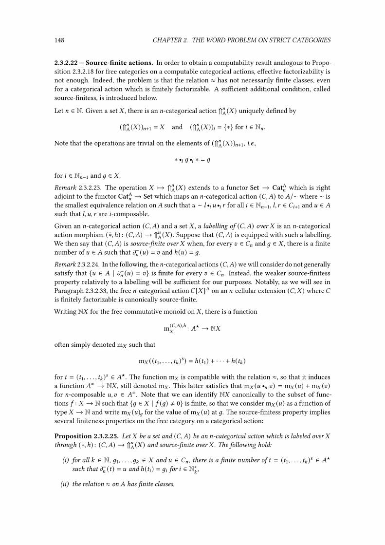
148 CHAPTER 2. THE WORD PROBLEM ON STRICT CATEGORIES

2.3.2.22 — Source-�nite actions. In order to obtain a computability result analogous to Propo-sition 2.3.2.18 for free categories on a computable categorical actions, e�ective factorizability isnot enough. Indeed, the problem is that the relation ≈ has not necessarily �nite classes, evenfor a categorical action which is �nitely factorizable. A su�cient additional condition, calledsource-�nitess, is introduced below.

Let = ∈ N. Given a set - , there is an =-categorical action ⇑=A(- ) uniquely de�ned by

(⇑=A(- ))=+1 = - and (⇑=A(- ))8 = {∗} for 8 ∈ N= .

Note that the operations are trivial on the elements of (⇑=A(- ))=+1, i.e.,

∗ r8 6 r

8 ∗ = 6

for 8 ∈ N=−1 and 6 ∈ - .

Remark 2.3.2.23. The operation - ↦→ ⇑=A(- ) extends to a functor Set → CatA= which is rightadjoint to the functor CatA= → Set which maps an =-categorical action (�,�) to �/∼ where ∼ isthe smallest equivalence relation on� such that D ∼ ; r8 D r

8 A for all 8 ∈ N=−1, ;, A ∈ �8+1 and D ∈ �such that ;, D, A are 8-composable.

Given an =-categorical action (�,�) and a set - , a labelling of (�,�) over - is an =-categoricalaction morphism (∗, ℎ) : (�,�) → ⇑=A(- ). Suppose that (�,�) is equipped with such a labelling.We then say that (�,�) is source-�nite over - when, for every E ∈ �= and 6 ∈ - , there is a �nitenumber of D ∈ � such that m−= (D) = E and ℎ(D) = 6.

Remark 2.3.2.24. In the following, the=-categorical actions (�,�)we will consider do not generallysatisfy that {D ∈ � | m−= (D) = E} is �nite for every E ∈ �= . Instead, the weaker source-�nitessproperty relatively to a labelling will be su�cient for our purposes. Notably, as we will see inParagraph 2.3.2.33, the free =-categorical action� [- ]A on an =-cellular extension (�,- ) where�is �nitely factorizable is canonically source-�nite.

Writing N- for the free commutative monoid on - , there is a function

m(�,�),ℎ-

: �★→ N-

often simply denoted m- such that

m- ((C1, . . . , C: )s) = ℎ(C1) + · · · + ℎ(C: )

for C = (C1, . . . , C: )s ∈ �★. The function m- is compatible with the relation ≈, so that it inducesa function �≈ → N- , still denoted m- . This latter satis�es that m- (D r

= E) = m- (D) + m- (E)for =-composable D, E ∈ �≈. Note that we can identify N- canonically to the subset of func-tions 5 : - → N such that {6 ∈ - | 5 (6) ≠ 0} is �nite, so that we consider m- (D) as a function oftype - → N and write m- (D)6 for the value of m- (D) at 6. The source-�nitess property impliesseveral �niteness properties on the free category on a categorical action:

Proposition 2.3.2.25. Let - be a set and (�,�) be an =-categorical action which is labeled over -through (∗, ℎ) : (�,�) → ⇑=A(- ) and source-�nite over - . The following hold:

(i) for all : ∈ N, 61, . . . , 6: ∈ - and D ∈ �= , there is a �nite number of C = (C1, . . . , C: )s ∈ �★

such that m−= (C) = D and ℎ(C8) = 68 for 8 ∈ N∗: ,

(ii) the relation ≈ on � has �nite classes,

2.3. COMPUTABLE FREE EXTENSIONS 149

(iii) if (�,�) is �nitely factorizable, then � [�]≈ is �nitely factorizable.

Proof. Proof of (i): We do an induction on the length : . There is only one C of length 0 suchthat m−= (C) = D. Now, suppose that the property holds for some : ∈ N. We prove that it holdsfor : + 1. Let 61, . . . , 6:+1 ∈ - , D ∈ �= and C = (C1, . . . , C:+1)s ∈ �★ be such that m−= (C) = D

and ℎ(C8) = 68 for 8 ∈ N∗:+1. Since m−= (C1) = D and ℎ(C1) = 61 and (�,�) is source-�nite, there is a �-

nite number of possible C1. For each of these, by putting C ′ = (C2, . . . , C:+1)s, we have m−= (C ′) = m+= (C1),thus, by induction hypothesis, there is a �nite number of possible C ′, which concludes (i).

Proof of (ii): Let D ∈ �≈, and : ∈ N and C = (C1, . . . , C: )s ∈ �★ be such that ÈCÉ = D. We havethat m- (D) = ℎ(C1) + · · · + ℎ(C: ), so there is a �nite number of possible tuples (ℎ(C1), . . . , ℎ(C: ))relatively to D. Hence, by (i), there is a �nite number of possible C .

Proof of (iii): Let D ∈ �≈. Consider E ∈ �= and F ∈ �≈ such that D = E r=−1 F . Let : ∈ N

and C1, . . . , C: ∈ � such thatF = È(C1, . . . , C: )sÉ. Then,

D = È(E r=−1 C1, . . . , E r

=−1 C: )sÉ.

By (ii), there is a �nite number of possible values for (E r=−1C1, . . . , E r=−1C: )s ∈ �★, and, since (�,�)is �nitely factorizable, there is a �nite number of possible pairs (E, (C1, . . . , C: )). Hence, there isa �nite number of pairs (E,F) ∈ �= × �≈ such that D = E r

=−1 F , and, similarly, there are a�nite number of pairs (E,F) ∈ �≈ × �= such that D = E r

=−1 F . Now consider E,F ∈ �≈ suchthat D = E r

= F . Let :, ; ∈ N and B1, . . . , B: and C1, . . . , C; in � be such that E = È(B1, . . . , B: )sÉandF = È(C1, . . . , C; )sÉ. Then,

D = È(B1, . . . , B: , C1, . . . , C; )sÉ.

Using (ii), we conclude similarly that there is a �nite number of pairs (E,F) ∈ �≈ × �≈ suchthat D = E r

= F . Hence, � [�]≈ is �nitely factorizable. �

2.3.2.26 — Computability of free categories on actions. With source-�niteness, we can de-duce computability properties for free categories on categorical actions. Let = ∈ N, - be a setand (�,�) be an =-categorical action labeled over - through (∗, ℎ) : (�,�) → ⇑=A(- ) and source-�nite over - , and E (�,�) be an injective and decidable encoding of (�,�) such that (�,�) iscomputable and e�ectively factorizable. We introduce �rst an encoding for�★ with the followingproperty:

Proposition 2.3.2.27. The following hold:

(i) there is an injective and decidable encoding E�★ of �★,

(ii) the function which maps D ∈ � to (D)s ∈ �★ is computable,

(iii) the function which maps D ∈ �= to ( )sD ∈ �★ is computable,

(iv) for 8 ∈ N=−1, the function which maps

(D, E) ∈ �★ ×8 �8+1 t�8+1 ×8 �★

to D r8 E is computable,

(v) the function which maps(D, E) ∈ �★ ×= �★

to D r= E is computable.

150 CHAPTER 2. THE WORD PROBLEM ON STRICT CATEGORIES

Proof. The set�★ is canonically isomorphic to�= t�′ where�= is in bijection with the identitiesof �★, and �′ is the subset of �<l consisting of non-empty sequences of =-composable elementsof �. Thus, we derive an encoding E�★ of �★ using the standard derivations of encodings for�nite sequences, subsets and disjoint union, and E�★ is injective since E�= and E� are. Moreover,since (�,�) is computable and E (�,�) is injective and decidable, �′ is a decidable subset of �<l ,so that E�★ is moreover decidable. Thus, (i) holds. By the de�nition of E�★ , (ii) holds. Moreover,by the de�nitions of id=+1(−) and the compositions r

8 and r= on �★ given in Section 2.2.4, (iii), (iv)

and (v) hold. �

Remark 2.3.2.28. If�0t· · ·t�= and� are encoded by datatypes cell and top_cell respectively,then, by the proof of Proposition 2.3.2.27(i) the set �★ is naturally encoded by the datatype

type seq =| SeqZ of cell (* constructor for zero-length sequences *)| SeqP of top_cell list (* constructor for positive-length sequences *)

and the computable function which witnesses that the encoding�★ is decidable can be representedby an OCaml function check_seq : seq -> bool .We now show that �≈ admits an injective and decidable encoding, using the method given byProposition 2.3.1.31. For this purpose, we �rst prove:

Proposition 2.3.2.29. The relation ≈1 on �★ is e�ectively right-�nite.

Proof. By the de�nition of ≈1, it is enough to show that the function which takes an input an=-composable pair (;, ; ′) ∈ �2 and outputs the �nite set of pairs (A, A ′) ∈ �2 such thatX(;, ; ′, A , A ′),is computable. The latter set is indeed �nite by Proposition 2.3.2.25(ii) since (;, ; ′)s ≈ (A, A ′)s.So let (;, ; ′) ∈ � be a pair of =-composable elements. Since (�,�) ∈ CatA= is computable ande�ectively factorizable, and E (�,�) is injective, we can compute all the pairs (D, E) ∈ �2 suchthat D, E are (=−1)-composable and satisfy

; = D r=−1 m

−= (E) and ; ′ = m+= (D) r=−1 E

and, for each such pair, we can compute the pair (A, A ′) where

A = m−= (D) r=−1 E and A ′ = D r=−1 m

+=−1(E).

Hence, we can compute all the pairs (A, A ′) such that X(;, ; ′, A , A ′) which concludes the proof. �

We can now deduce the computability of � [�]≈:

Proposition 2.3.2.30. The following hold:

(i) there is an injective and decidable encoding E�≈ of �≈,

(ii) the function È−É : �★→ �≈ is computable,

(iii) the function which maps D ∈ � to È(D)sÉ ∈ �≈ is computable,

(iv) the function which maps D ∈ �= to id=+1D ∈ �≈ is computable,

(v) for 8 ∈ N=−1, the function which maps

(D, E) ∈ �≈ ×8 �8+1 t�8+1 ×8 �≈

to D r8 E is computable,

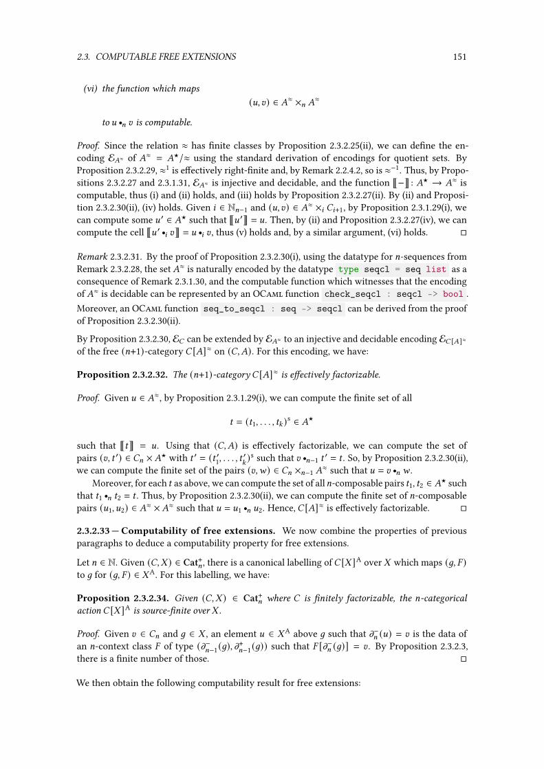
2.3. COMPUTABLE FREE EXTENSIONS 151

(vi) the function which maps(D, E) ∈ �≈ ×= �≈

to D r= E is computable.

Proof. Since the relation ≈ has �nite classes by Proposition 2.3.2.25(ii), we can de�ne the en-coding E�≈ of �≈ = �★/≈ using the standard derivation of encodings for quotient sets. ByProposition 2.3.2.29, ≈1 is e�ectively right-�nite and, by Remark 2.2.4.2, so is ≈−1. Thus, by Propo-sitions 2.3.2.27 and 2.3.1.31, E�≈ is injective and decidable, and the function È−É : �★ → �≈ iscomputable, thus (i) and (ii) holds, and (iii) holds by Proposition 2.3.2.27(ii). By (ii) and Proposi-tion 2.3.2.30(ii), (iv) holds. Given 8 ∈ N=−1 and (D, E) ∈ �≈ ×8 �8+1, by Proposition 2.3.1.29(i), wecan compute some D ′ ∈ �★ such that ÈD ′É = D. Then, by (ii) and Proposition 2.3.2.27(iv), we cancompute the cell ÈD ′ r8 EÉ = D r

8 E , thus (v) holds and, by a similar argument, (vi) holds. �

Remark 2.3.2.31. By the proof of Proposition 2.3.2.30(i), using the datatype for =-sequences fromRemark 2.3.2.28, the set �≈ is naturally encoded by the datatype type seqcl = seq list as aconsequence of Remark 2.3.1.30, and the computable function which witnesses that the encodingof �≈ is decidable can be represented by an OCaml function check_seqcl : seqcl -> bool .Moreover, an OCaml function seq_to_seqcl : seq -> seqcl can be derived from the proofof Proposition 2.3.2.30(ii).

By Proposition 2.3.2.30, E� can be extended by E�≈ to an injective and decidable encoding E� [�]≈of the free (=+1)-category � [�]≈ on (�,�). For this encoding, we have:

Proposition 2.3.2.32. The (=+1)-category � [�]≈ is e�ectively factorizable.

Proof. Given D ∈ �≈, by Proposition 2.3.1.29(i), we can compute the �nite set of all

C = (C1, . . . , C: )s ∈ �★

such that ÈCÉ = D. Using that (�,�) is e�ectively factorizable, we can compute the set ofpairs (E, C ′) ∈ �= ×�★ with C ′ = (C ′1, . . . , C ′: )

s such that E r=−1 C

′ = C . So, by Proposition 2.3.2.30(ii),we can compute the �nite set of the pairs (E,F) ∈ �= ×=−1 �

≈ such that D = E r= F .

Moreover, for each C as above, we can compute the set of all=-composable pairs C1, C2 ∈ �★ suchthat C1 r

= C2 = C . Thus, by Proposition 2.3.2.30(ii), we can compute the �nite set of =-composablepairs (D1, D2) ∈ �≈ ×�≈ such that D = D1 r

= D2. Hence, � [�]≈ is e�ectively factorizable. �

2.3.2.33 — Computability of free extensions. We now combine the properties of previousparagraphs to deduce a computability property for free extensions.

Let = ∈ N. Given (�,- ) ∈ Cat+= , there is a canonical labelling of� [- ]A over - which maps (6, � )to 6 for (6, � ) ∈ -A. For this labelling, we have:

Proposition 2.3.2.34. Given (�,- ) ∈ Cat+= where � is �nitely factorizable, the =-categoricalaction � [- ]A is source-�nite over - .

Proof. Given E ∈ �= and 6 ∈ - , an element D ∈ -A above 6 such that m−= (D) = E is the data ofan =-context class � of type (m−=−1(6), m+=−1(6)) such that � [m−= (6)] = E . By Proposition 2.3.2.3,there is a �nite number of those. �

We then obtain the following computability result for free extensions:

152 CHAPTER 2. THE WORD PROBLEM ON STRICT CATEGORIES

Proposition 2.3.2.35. Let = ∈ N, (�,- ) ∈ Cat+= and E (�,- ) be an injective and decidable encodingof (�,- ) such that (�,- ) is computable and� e�ectively factorizable. Then, there is an injective anddecidable encoding E� [- ] of the (=+1)-category� [- ] that extends E� such that� [- ] is computableand e�ectively factorizable. Moreover, the canonical embedding - → � [- ]=+1 is computable.

Proof. The encoding E� [- ]=+1 of � [- ]=+1 is constructed using Propositions 2.3.2.18, 2.3.2.21,2.3.2.30 and 2.3.2.34, so that, by extending E� with E� [- ]=+1 , we obtain an encoding of � [- ]which makes� [- ] computable and moreover comptationally factorizable by Proposition 2.3.2.32.Moreover, the embedding - → � [- ]=+1 is computable by Proposition 2.3.2.20 and Proposi-tion 2.3.2.30(iii). �

Remark 2.3.2.36. By inspecting the constructive content of the proof of Proposition 2.3.2.35 andof the propositions it uses, we have in fact proved a stronger statement: for = ∈ N, there is acomputable function which takes as inputs

– a code for a computable =-cellular extension (�,- ) that is equipped with an injective anddecidable encoding E (�,- ) ,

– codes of the computable functions that witness that � is e�ectively factorizable,

and which outputs

– a code for the (=+1)-category � [- ], which is equpipped with the injective and decidableencoding E� [- ] given by Proposition 2.3.2.35 that extends E� ,

– a code for the embedding - → � [- ]=+1.

Thus, we can consider that Proposition 2.3.2.35 is “e�ectively parametrized” by (�,- ) and thecomputable functions that witness that � is e�ectively factorizable.

2.3.3 The case of polygraphs

We now consider the special case of polygraphs and show that, when provided with an adequatecomputational description of those, the associated free strict categories are computable. Moreover,we introduce in this case an alternative procedure to compute the context class associated to acontext than the one provided by Proposition 2.3.2.7(ii), enabling faster recursive models for thosefree categories.

2.3.3.1 — Computable polygraphs. For = ∈ N and an =-polygraph P equipped with injectiveand decidable encodings EP8 of P8 for 8 ∈ N= , we de�ne by induction on = the property that P isa computable polygraph, together with a decidable and injective encoding EP∗ of the free =-cate-gory P∗, such that P∗ is computable and e�ectively factorizable for this encoding. A 0-polygraph Pis always computable and we take EP∗ = EP0 . Given = ∈ N, an (=+1)-polygraph P′ = (P, - ) iscomputable when P is and when the functions d−= , d

+= : - → P∗= are computable, relatively to the

encoding EP∗= of P∗= coming with the encoding EP∗ given by the induction. Moreover, we takefor E (P′)∗ the encoding given by Proposition 2.3.2.35. For these encodings, we have the followingcomputability property for free strict categories on computable polygraphs:

Proposition 2.3.3.2. Given = ∈ N and an =-polygraph P equipped with injective and decidableencodings EP8 of P8 for 8 ∈ N= such that P is computable, the =-category P∗ is computable and theembeddings P8 → P∗8 are computable for 8 ∈ N= .

Proof. By induction on =, using Proposition 2.3.2.35. �

2.3. COMPUTABLE FREE EXTENSIONS 153

2.3.3.3 — More e�cient computation of the equivalences classes. Let = ∈ N with = ≥ 2and � be an =-category equipped with an injective and decidable encoding E (�,- ) , such that �is computable and e�ectively factorizable for this encoding. Recall that we de�ned in the proofof Proposition 2.3.2.11 an algorithm which, given an<-context � of � for some< ∈ N= as input,and output È�É. This algorithm is derived by Proposition 2.3.1.31 using the de�nition of ≈1

< , butother algorithms are possible. For concrete applications like the word problem below, it is impor-tant that the algorithm that executes this operation is fast, since it is part of the implementationsof the composition operations r

8 (c.f. Proposition 2.3.2.18). One way to obtain a faster algorithmis to use a more suitable relation ≈1

< that generates ≈< as a re�exive transitive closure, so thatthe algorithm derived by Proposition 2.3.1.31 is more e�cient (when � allows it). We give suchan alternative generating relation in the case where � = P∗ for some computable =-polygraph Pby re�ning a bit the axioms used to de�ne ≈1

< .So let P be an =-polygraph and< ∈ N= . We de�ne a relation ≈< between<-contexts of the

same type of P∗. Given an<-type (D,D ′) and two<-contexts of type (D,D ′)

�1 = (;1, �1, A1) and �2 = (;2, �2, A2)

we write �1 ≈< �2 when there exists (<−1)-contexts (; ′8 , � ′8 , A ′8 ) such that È(; ′8 , � ′8 , A ′8 )É = �8for 8 ∈ {1, 2}, and ;,F, A ∈ P∗< with |F | = 1 (recall the notion of length de�ned in Paragraph 2.2.4.1)and such that either the set of conditions (≈-L) or (≈-R) (the ones de�ning ≈1

<) is satis�ed. Notethat the only di�erence between the de�nitions of ≈1

< and≈1< is that we requireF to be of length 1.

We verify that:

Proposition 2.3.3.4. The re�exive symmetric transitive closure of ≈1< is ≈< .

Proof. Let ≈< be the re�exive symmetric transitive closure of ≈1< . Since we have ≈1

< ⊆ ≈1< , it is

enough to show that ≈1< ⊆ ≈< . Let (D,D ′) be an<-type and

�1 = (;1, �1, A1) and �2 = (;2, �2, A2)

be two <-contexts of type (D,D ′) of P∗ such that �1 ≈1< �2. By de�nition of ≈1

< , there exist(<−1)-contexts (; ′8 , � ′8 , A ′8 ) such that È(; ′8 , � ′8 , A ′8 )É = �8 for 8 ∈ {1, 2}, and ;,F, A ∈ P∗< such that ei-ther (≈-L) or (≈-R) is satis�ed. By symmetry, suppose that (≈-L) is satis�ed. We prove that �1 ≈ �2by induction on the length |F | ofF . If |F | = 0, thenF = idF for some F ∈ P∗<−1, so that �1 = �2,thus �1 ≈< �2. If |F | = 1, then �1 ≈1

< �2 by de�nition of ≈1< . Otherwise, suppose that |F | = : + 1

for some : ∈ N∗. Then, by the de�nition of the functor −[−]≈, we have that F = F ′ r= F ′′ forsomeF ′,F ′′ ∈ P∗< such that |F ′ | = 1 and |F ′′ | = : . Note that

(F ′ r<−1 F′′) r<−2 �

′1 [D] r<−2 A

′1 = (F ′ r<−2 �

′1 [D] r<−2 A

′1) r<−1 (F ′′ r<−2 �

′1 [D] r<−2 A

′1)

so that, by induction hypothesis, we have �1 ≈< �3 where �3 = (;3, �3, A3) is an <-context oftype (D,D ′) with �3 = È(; ′3, � ′3, A ′3)É for some (<−1)-context (; ′3, � ′3, A ′3) de�ned by � ′3 = �

′1 and

; ′3 = m−<−1(F ′′) A ′3 = A

′1

;3 = ; r<−1 (F ′ r<−2 �′1 [D] r<−2) A3 = (F ′′ r<−2 �

′1 [D ′] r<−2 A

′1) r<−1 A .

Thus, we also have �3 ≈1< �2, so that �1 ≈< �2. Hence, ≈< = ≈< . �

Remark 2.3.3.5. We can do a remark similar to Remark 2.2.2.4. Given< ∈ N= , the relation ≈−1<

on the<-context, which is de�ned by �1 ≈−1< �2 if and only if �2 ≈1

< �1 for all<-contexts �1, �2of the same <-type, admits a de�nition by axioms (≈-L)’ and (≈-R)’ which are symmetricalto (≈-L) and (≈-R). Moreover, ≈< can be equivalently described as the re�exive transitive closureof ≈1

< ∪ ≈−1< , so that, in the proofs, by symmetry of the de�nitions of ≈1

< and ≈−1< , we can often

reduce a case analysis of �1 ≈< �2 to �1 ≈1< �2.

154 CHAPTER 2. THE WORD PROBLEM ON STRICT CATEGORIES

Now, suppose that P is equipped with injective and decidable encodings EP8 of P8 for 8 ∈ N= andthat P is computable for these encodings, so that, by the de�nition of “computable” for polygraphs,we derive an injective and decidable encoding EP∗ of P∗ for which P∗ is computable and e�ectivelyfactorizable. For this encoding, we have:

Proposition 2.3.3.6. Given< ∈ N= with< ≥ 2, the function which takes as input an<-cellD ∈ P∗< ,and outputs the �nite set of (<−1)-composable pairs (E,F) ∈ (P∗<)2 such that D = E r

<−1 F

and |F | = 1, is computable.

Proof. Let D ∈ P∗< . Consider E,F ∈ P∗< such that D = E r<−1 F . Then, by putting � = P∗<−1

and � = (P<)A, we have E = ÈBÉ andF = ÈCÉ for some :, ; ∈ N and

B = (B1, . . . , B: )s and C = (C1, . . . , C; )s

in �★. Since |F | = 1, we have ; = 1. Moreover, we deduce that D = È(B1, . . . , B: , C1)sÉ. ByProposition 2.3.1.29(i), we can compute the set of possible representants (B1, . . . , B: , C1)s ∈ �★ of D.For each possible value, by Proposition 2.3.2.30(ii), we can compute the codes of E = È(B1, . . . , B: )sÉandF = È(C1)sÉ, which concludes the proof. �

Hence, we get another proof of Proposition 2.3.2.11:

Proposition 2.3.3.7. For every < ∈ N= , D ∈ �< and D ′ = (m−<−1(D), m+<−1(D)), the restrictionof ≈< to<-contexts of instantiable types is e�ectively right-�nite, and the function which maps an<-context � of type D ′ to È�É is computable.

Proof. By Proposition 2.3.1.31, it is su�cient to prove that the restriction of ≈1< ∪ ≈1

< to<-con-texts of instantiable type is e�ectively right-�nite. By Remark 2.3.3.5, it is enough to show thatthe restriction of ≈1 is e�ectively right-�nite. Using Proposition 2.3.3.6, the proof of the latterproperty is similar to the one of Proposition 2.3.2.10. �

However, the instance of the algorithm of Proposition 2.3.1.31 using the e�ectively right-�nite ≈1<

will be more e�cient than the one using ≈1< . Indeed, given< ∈ N= and an<-context �, we have

{� ′ | � ′<-context such that � ≈1< � ′} ⊆ {� ′ | � ′<-context such that � ≈1

< � ′}

by de�nition of ≈1< and ≈1

< . Thus, intuitively, we iterate on less<-context � ′ per<-context � inthe algorithm of Proposition 2.3.1.31 when using ≈1

< than when using ≈1< .

2.4 Word problem on polygraphs

We now use the computability results of the previous sections to give a solution to the wordproblem on polygraphs of strict categories. Our solution is strongly inspired from the one givenby Makkai in [Mak05]. However, whereas Makkai deemed his procedure “infeasible” in practice,the one we propose admits a relatively fast implementation, that solves rapidly most instances ofthe word problem.

We �rst give a precise statement to this problem after introducing terms on polygraphs (Sec-tion 2.4.1). Then, we give a solution to the word problem on the special case of �nite polygraphs(Section 2.4.2). By Proposition 2.3.3.2, we can already compute recursive models with injectiveencodings for the free strict categories on computable polygraphs and, in particular, �nite poly-graphs, so that the word problem is already essentially solved since one can compare two termsby comparing the codes of their evaluations in the recursive models. But one hardly writes down

2.4. WORD PROBLEM ON POLYGRAPHS 155

a code for a computable polygraph, because of its intrinsically inductive de�nition. Thus, most ofour concerns will be to de�ne a user-friendly way to use polygraphs as inputs of programs. Next,we show how to extend our method to more general polygraphs (possible in�nite, possibly notcomputable). Finally, we illustrate the discussion of this section by providing an implementationin OCaml (Section 2.4.4).

2.4.1 Terms and word problem

Here, we de�ne the terms on polygraphs and give a precise statement to the word problem onpolygraphs.

2.4.1.1 — Terms on polygraphs. Let = ∈ N ∪ {l}. Given an =-polygraph P, for : ∈ N= , wede�ne the sets of :-terms T P

:of P inductively as follows:

– given : ∈ N= and 6 ∈ P: , there is a :-term gen: (6) ∈ T P:,

– given : ∈ N=−1 and a :-term C ∈ T P:, there is a (:+1)-term id:+1

:(C) ∈ T P

:+1,

– given 8, : ∈ N= with 8 < : and :-terms C1, C2 ∈ T P:, there is a :-term C1 ∗8,: C2 ∈ T P

:.

We write T P = t:∈N= T P:

for the set of all terms of P. Given a morphism � : P→ Q ∈ Pol= , thereis a function

T � : T P → TQ

de�ned on C ∈ T P by induction on C :

– for : ∈ N= and 6 ∈ P: , T � (gen: (6)) = gen: (� (6)),

– for : ∈ N=−1 and a :-term C , T � (id:+1:(C)) = id:+1

:(T � (C)),

– for 8, : ∈ N= with 8 < : and :-terms C1, C2, T � (C1 ∗8,: C2) = T � (C1) ∗8,: T � (C2).

We now de�ne subsetsWP:

of T P:

consisting of the :-terms that are well-typed, together with anevaluation function

È−ÉP:

: WP:→ P∗

:

by induction on : ∈ N= . All 0-terms are well-typed and are of the form gen0(6) for some 6 ∈ P0and we put Ègen0(6)ÉP: = 6. For : ∈ N∗= , a :-term is well-typed when there exist D, E ∈ P∗

:−1 suchthat there is a derivation `P

:C : D → E , with `P

:de�ned below:

– given 6 ∈ P: , we have `P:

gen: (6) : d−:−1(6) → d+

:−1(6),

– given a well-typed (:−1)-term C , we have `P:

id::−1(C) : ÈCÉ

P:−1 → ÈCÉ

P:−1,

– given 8 ∈ N:−2 and :-terms C1, C2 such that `P:C1 : D1 → D ′1 and `P

:C2 : D2 → D ′2 for

some D1, D′1, D2, D

′2 ∈ P∗:−1 with m+8 (D1) = m−8 (D2), we have `P

:C1 ∗8,: C2 : D1 ∗8 D2 → D ′1 ∗8 D ′2,

– given :-terms C1, C2 such that `P:C1 : D1 → D2 and `P

:C2 : D2 → D3 for some D1, D2, D3 ∈ P∗:−1,

we have `P:C1 ∗:−1,: C2 : D1 → D3.

We then easily verify the following property by induction on C :

Proposition 2.4.1.2. Given C ∈ WP:, the following hold:

(i) there are unique D,D ′ ∈ P∗:−1 such that `P

:C : D → D ′ is derivable,

156 CHAPTER 2. THE WORD PROBLEM ON STRICT CATEGORIES

(ii) the derivation `P:C : D → D ′ is unique,

(iii) mn:−2(D) = m

n:−2(D

′) for n ∈ {−, +}.

Given a well-typed :-term C with associated derivation `P:C : D → D ′, we de�ne a cell ÈCÉP

:∈ P∗

:

such that m−:−1(ÈCÉ

P:) = D and m+

:−1(ÈCÉP:) = D ′ by induction on the derivation of C :

– if C = gen: (6) for some 6 ∈ P: , then ÈCÉP:= 6,

– if C = id::−1(C) for some C ∈ T P

:−1, then ÈCÉP:= id:ÈCÉP

:

,

– if C = C1 ∗8,: C2 for some 8 ∈ N:−1 and C1, C2 ∈ T P:, then ÈCÉP

:= ÈC1ÉP: ∗8 ÈC2É

P:.

Note that the well-typedness of C ensures that È−ÉP:

is well-de�ned, which concludes the inductivede�nition ofWP

:and È−ÉP

:. We writeWP for t:∈N=WP

:. The above evaluation functions of well-

typed :-terms de�ne a functionÈ−ÉP : WP → P∗.

Given a morphism � : P→ Q in Pol= , the function T � restricts to a functionW� : WP →WQ .We then have the following naturality property:

Proposition 2.4.1.3. Given a morphism � : P→ Q in Pol= ,

È−ÉQ ◦W� = � ∗ ◦ È−ÉP.

Proof. Given C ∈ WP, we prove by induction on C that ÈW� (C)ÉQ = � ∗(ÈCÉP):

– if C = gen: (6) for some : ∈ N= and 6 ∈ P: ,

ÈW� (C)ÉQ = � (6) = � ∗ ◦ ÈCÉP,

– if C = id:+1:(C) for some : ∈ N=−1 and C ∈ T P

:, then,

ÈW� (C)ÉQ = Èid:+1:(W� (C))ÉQ

= id:+1:(ÈW� (C)ÉQ)

= id:+1:(� ∗(ÈCÉQ)) (by induction hypothesis)

= � ∗(id:+1:(ÈCÉQ))

= � ∗(ÈCÉQ),

– if C = C1 ∗8,: C2 for some 8, : ∈ N= with 8 < : and C1, C2 ∈ WP:

, then,

ÈW� (C)ÉQ = ÈW� (C1) ∗8,:W� (C2)ÉQ

= ÈW� (C1)ÉQ ∗8 ÈW� (C2)ÉQ

= � ∗(ÈC1ÉP) ∗8 � ∗(ÈC2ÉP) (by induction hypothesis)= � ∗(ÈC1ÉP ∗8 ÈC2ÉP)= � ∗(ÈCÉP). �

2.4.1.4 —Word problem statement. For = ∈ N ∪ {l} an =-polygraph P, the word problem on Pconsists, given : ∈ N= and C1, C2 ∈ WP

:, in deciding whether ÈC1ÉP = ÈC2ÉP. By “deciding”, we

mean exhibiting a procedure parametrized by P, =, :, C1 and C2 that terminates in a �nite numberof steps and such that this procedure returns “yes” if and only if ÈC1ÉP = ÈC2ÉP and returns “no”otherwise. It is desirable that most of the steps of this procedure be implementable on a computer.

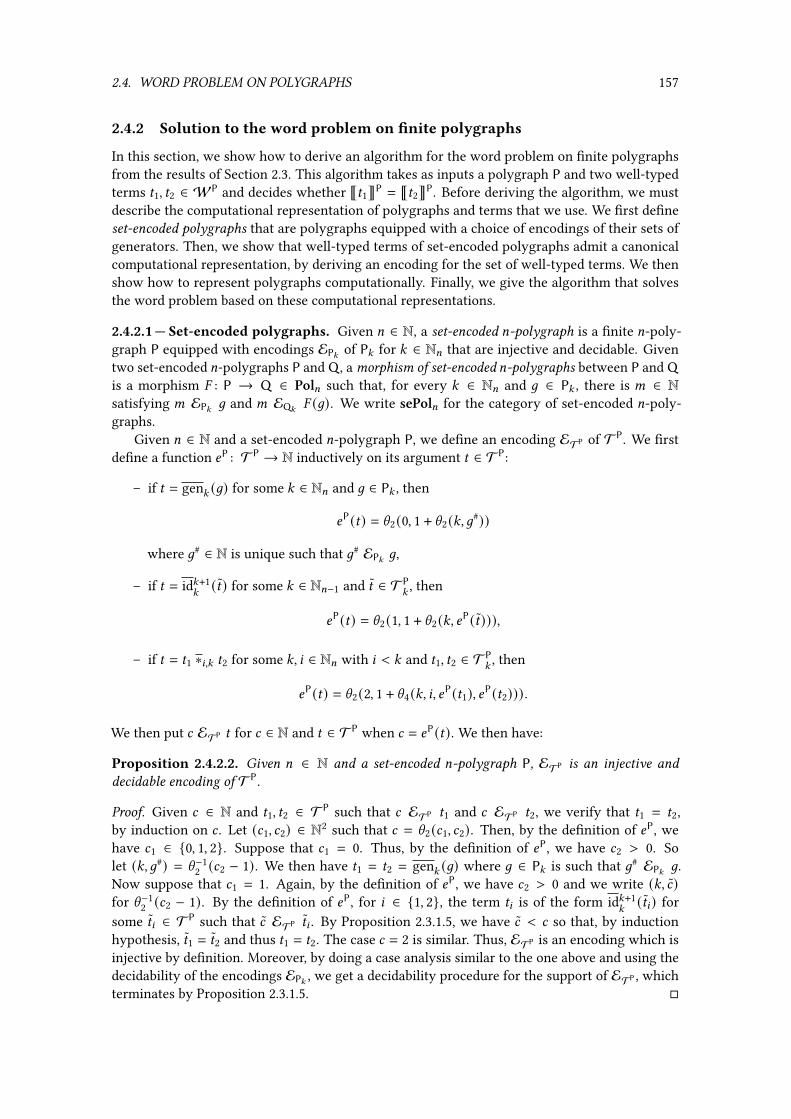
2.4. WORD PROBLEM ON POLYGRAPHS 157

2.4.2 Solution to the word problem on �nite polygraphs

In this section, we show how to derive an algorithm for the word problem on �nite polygraphsfrom the results of Section 2.3. This algorithm takes as inputs a polygraph P and two well-typedterms C1, C2 ∈ WP and decides whether ÈC1ÉP = ÈC2ÉP. Before deriving the algorithm, we mustdescribe the computational representation of polygraphs and terms that we use. We �rst de�neset-encoded polygraphs that are polygraphs equipped with a choice of encodings of their sets ofgenerators. Then, we show that well-typed terms of set-encoded polygraphs admit a canonicalcomputational representation, by deriving an encoding for the set of well-typed terms. We thenshow how to represent polygraphs computationally. Finally, we give the algorithm that solvesthe word problem based on these computational representations.

2.4.2.1 — Set-encoded polygraphs. Given = ∈ N, a set-encoded =-polygraph is a �nite =-poly-graph P equipped with encodings EP: of P: for : ∈ N= that are injective and decidable. Giventwo set-encoded =-polygraphs P and Q , a morphism of set-encoded =-polygraphs between P and Qis a morphism � : P → Q ∈ Pol= such that, for every : ∈ N= and 6 ∈ P: , there is < ∈ Nsatisfying < EP: 6 and < EQ: � (6). We write sePol= for the category of set-encoded =-poly-graphs.

Given = ∈ N and a set-encoded =-polygraph P, we de�ne an encoding ETP of T P. We �rstde�ne a function 4P : T P → N inductively on its argument C ∈ T P:

– if C = gen: (6) for some : ∈ N= and 6 ∈ P: , then

4P(C) = \2(0, 1 + \2(:,6#))

where 6# ∈ N is unique such that 6# EP: 6,

– if C = id:+1:(C) for some : ∈ N=−1 and C ∈ T P

:, then

4P(C) = \2(1, 1 + \2(:, 4P(C))),

– if C = C1 ∗8,: C2 for some :, 8 ∈ N= with 8 < : and C1, C2 ∈ T P:, then

4P(C) = \2(2, 1 + \4(:, 8, 4P(C1), 4P(C2))).

We then put 2 ETP C for 2 ∈ N and C ∈ T P when 2 = 4P(C). We then have:

Proposition 2.4.2.2. Given = ∈ N and a set-encoded =-polygraph P, ETP is an injective anddecidable encoding of T P.

Proof. Given 2 ∈ N and C1, C2 ∈ T P such that 2 ETP C1 and 2 ETP C2, we verify that C1 = C2,by induction on 2 . Let (21, 22) ∈ N2 such that 2 = \2(21, 22). Then, by the de�nition of 4P, wehave 21 ∈ {0, 1, 2}. Suppose that 21 = 0. Thus, by the de�nition of 4P, we have 22 > 0. Solet (:,6#) = \−1

2 (22 − 1). We then have C1 = C2 = gen: (6) where 6 ∈ P: is such that 6# EP: 6.Now suppose that 21 = 1. Again, by the de�nition of 4P, we have 22 > 0 and we write (:, 2)for \−1

2 (22 − 1). By the de�nition of 4P, for 8 ∈ {1, 2}, the term C8 is of the form id:+1:(C8) for

some C8 ∈ T P such that 2 ETP C8 . By Proposition 2.3.1.5, we have 2 < 2 so that, by inductionhypothesis, C1 = C2 and thus C1 = C2. The case 2 = 2 is similar. Thus, ETP is an encoding which isinjective by de�nition. Moreover, by doing a case analysis similar to the one above and using thedecidability of the encodings EP: , we get a decidability procedure for the support of ETP , whichterminates by Proposition 2.3.1.5. �

158 CHAPTER 2. THE WORD PROBLEM ON STRICT CATEGORIES

Remark 2.4.2.3. Given= ∈ N and an=-polygraph P, if P0t· · ·tP= is encoded by the datatype gen ,then the set T P is naturally encoded by the datatype

type term =| TermGen of int * gen| TermId of int * term| TermComp of (int * int * term * term)

We verify that the functions on terms derived from morphisms of set-encoded polygraphs arecompatible with the encodings on terms:

Proposition 2.4.2.4. Given = ∈ N, two set-encoded =-polygraphs P and Q and a morphism ofset-encoded =-polygraphs � : P → Q , for all 2 ∈ N and C ∈ T P, we have 2 ETP C if and onlyif 2 ETQ T � (C).

Proof. This is proved by induction on C . The only non-trivial case is when C = gen: (6) forsome : ∈ N= and 6 ∈ P: . By the de�nition of set-encoded =-polygraph morphism, we havethat, for all 2 ′ ∈ N, 2 ′ EP: 6 if and only if 2 ′ EQ: � (6). Hence, 2 ETP gen: (6) if and onlyif 2 ETQ gen: (� (6)). �

SinceWP is a subset of T P, we derive an injective encoding EWP forWP (but we do not knowthat it is decidable at the moment). We then have:

Proposition 2.4.2.5. Given = ∈ N and a set-encoded =-polygraph P, if P is computable, then

(i) the function È−ÉP is computable,

(ii) the encoding EWP is decidable.

Proof. Proof of (i): Remember that the encoding of P∗ is the one given by Proposition 2.3.3.2.The latter properties also states that P∗ is computable for these encodings and so are the em-beddings P: → P∗

:for : ∈ N= . Thus, the operations ∗8,: and id: are computable for 8, : ∈ N=

with 8 < : , so that the inductive de�nition of È−ÉP witnesses the fact that È−ÉP is computable.

Proof of (ii): Using (i), we give a procedure that decides, given 2 ∈ N, whether 2 EWP C forsome C ∈ WP. By Proposition 2.4.2.2, we can �rst decide whether 2 ETP C for some C ∈ T P. Then,we verify by induction on C that C ∈ WP using the following inductive veri�cation procedure:

– if C = gen: (6) for some : ∈ N= and 6 ∈ P: , then C ∈ WP,

– if C = id:+1:(C) for some : ∈ N=−1 and C ∈ T P

:, then C ∈ WP if and only if C ∈ WP,

– if C = C1 ∗8,: C2 for some 8, : ∈ N= with 8 < : , then C ∈ WP if and only if C1, C2 ∈ WP

and m+8 (ÈC1ÉP) = m−8 (ÈC2ÉP).

Note that the last condition “m+8 (ÈC1ÉP) = m−8 (ÈC2ÉP)” can be computationally veri�ed since È−ÉPis computable by (i), and P∗ is computable by Proposition 2.3.3.2 (thus so are the functions m−8 , m

+8 ),

and EP∗:

is injective. �

Remark 2.4.2.6. In the same spirit as Remark 2.3.2.36, we in fact proved the stronger statementthat Proposition 2.4.2.5 is “e�ectively parametrized” by P, i.e., there is a computable functionwhich takes as inputs

– the codes of the computable functions that decide the support of EP: for : ∈ N= ,

2.4. WORD PROBLEM ON POLYGRAPHS 159

– the codes of the computable functions that witness that P is computable,

and which outputs

– a code for the computable function È−ÉP,

– a code for the function that decides the support ofWP.

2.4.2.7 — Term de�nitions for polygraphs. In order to de�ne algorithms parametrized by�nite polygraphs, we need to de�ne an encodable structure that represents such polygraphs.The di�culty here lies in the fact that the de�nition of (=+1)-polygraphs depends on the free=-category construction to de�ne the source and target of the (=+1)-generators. An encodingfor such free =-category can be de�ned inductively using Proposition 2.3.2.35, but this encodingwould be terrible for practical purposes, since it would require a user to manipulate by handthe complicated internal encodings of Proposition 2.3.2.35. Instead, we de�ne a more naturalstructure that uses well-typed terms to de�ne the source and target of (=+1)-generators.

For = ∈ N, we de�ne the notion of =-term de�nition together with the set-encoded =-polygraphassociated to an =-term de�nition. A 0-term de�nition is a �nite subset �0 ⊂ N and the 0-poly-graph associated to �0 is � with �0 = �0 and E�0 induced by EN. For = ∈ N, an (=+1)-termde�nition is a dependent pair

� = ((� ′, (), (dt,−= , d

t,+= ))

where � ′ is an =-term de�nition, ( is a �nite subset of N, and dt,−= , d

t,+= are functions ( →W�′

=

such thatmn=−1(Èdt,−

= (6)É�′) = mn=−1(Èdt,+

= (6)É�′)

for n ∈ {−, +} and 6 ∈ ( . The set-encoded (=+1)-polygraph � associated to � is de�ned by

�≤= = � ′, �=+1 = ( and dn= (6) = Èdt,n= (6)É�

′

for n ∈ {−, +} and 6 ∈ �=+1. Finally, E�=+1 is the encoding induced by EN. For = ∈ N, wewrite D= for the set of =-term de�nitions. By induction on =, we de�ne an injective encodingon D= . We de�ne the encoding ED0 for D0 from the encoding EN using the standard derivationof encodings for �nite subsets. Given = ∈ N, we de�ne the encoding ED=+1 for D=+1 using thestandard derivation of encodings for dependent pairs where

– the encoding for the pairs (� ′, () is de�ned with the standard derivation of encodings forpairs using ED= and EPf (N) ,

– given a pair (� ′, (), the encoding for the pairs (dt,−= , d

t,+= ) is de�ned with the standard

derivations of encodings for pairs and functions with �nite domains, using, for domain andcodomain of dt,−

= and dt,+= , the encodings E( (induced by EN) and EW�′ respectively.

Remark 2.4.2.8. By Remarks 2.3.1.23 and 2.3.1.27, using the datatype for terms from Remark 2.4.2.3with gen = int , the set t=∈N D= is naturally encoded by the datatype

type term_def =| TermDefZ of int list| TermDefS of term_def * int list * (int * term) list * (int * term) list

Up to isomorphism, term de�nitions encode all �nite set-encoded polygraphs:

160 CHAPTER 2. THE WORD PROBLEM ON STRICT CATEGORIES

Proposition 2.4.2.9. Given = ∈ N and a �nite set-encoded =-polygraph P, there exists an =-termde�nition � ∈ D= and an isomorphism P → � in sePol= . Moreover, � and the isomorphism doesnot depend on � .

Proof. We prove this property by induction on=. If= = 0, then there is a unique� ∈ D0 such that Pis isomorphic to � in sePol= , which is such that�0 is the support of EP0 . So suppose that the prop-erty holds for some = ∈ N. We show that it holds for =+1. Let P be a �nite set-encoded (=+1)-poly-graph. By induction, there is � ′ ∈ D= and an isomorphism � : P≤= → � ′ in sePol= . We nowde�ne the (=+1)-term � = ((� ′, (), (dt,−

= , dt,+= )) ∈ D=+1 and 5 : P=+1 → ( such that (�, 5 ) : P→ �

is an isomorphism in sePol=+1. By the constraints imposed on the morphisms of sePol=+1 andsince E( is the canonical encoding of the subset ( ⊂ N, we necessarily have that ( is the supportof EP=+1 and 5 maps 6 ∈ P=+1 to the unique 6# ∈ ( such that 6# EP=+1 6. For such ( and 5 , we de-�ne dt,n

= for n ∈ {−, +} by choosing =-terms C−6 , C+6 ∈ W%≤= such that ÈCn6É%≤= = dn= (6) for 6 ∈ P=+1(that exist by Proposition 1.4.1.16), and we put dt,n

= (5 (6)) =W� (Cn6 ). Thus, for 6 ∈ P=+1, we have

dn= (5 (6)) = ÈW� (Cn6 )É�′

= � ∗(ÈCn6É%≤= ) (by Proposition 2.4.1.3)

= � ∗(dn= (6))

so that (�, 5 ) is a morphism of sePol=+1 which is moreover an isomorphism. By induction hypoth-esis, � ′ and the isomorphism � does not depend on � ′, and ( and the bijection 5 : P=+1 → ( areuniquely de�ned from P=+1 and EP=+1 . Moreover, the functions d−= , d

+= : �=+1 → �∗= are uniquely

de�ned from P, � and 5 sincedn= (5 (6)) = � ∗(dn= (6))

so that neither � nor (�, 5 ) : P=+1 → � depends on � . �

Moreover, the polygraphs associated to term de�nitions have the required computability proper-ties to solve the word problem:

Proposition 2.4.2.10. Given = ∈ N and � ∈ D= ,

(i) � is computable,

(ii) the function È−É� : W� → �∗ is computable,

(iii) the encoding EW� is decidable.

Proof. We prove the property by induction on =. When = = 0, the property holds. So supposethat the property holds for some = ∈ N. We show that it holds for = + 1.

Proof of (i): Let � = (� ′, (, dt,−= , d

t,+= ) be an (=+1)-term de�nition. By induction hypothesis,

the =-polygraph � ′ is computable. Moreover, note that the functions dt,−= , d

t,+= are computable:

for n ∈ {−, +}, the value of dt,n= at some 6 ∈ ( can be computed by searching for the unique

pair (6, C) with C ∈ W�′ in the graph of dt,n= (which is part of the code of �). By the induction

hypothesis, È−É�′ : W�′ → (� ′)∗ is computable, so that dn= = È−É�′ ◦ dt,n= : �=+1 → �∗= is

computable for n ∈ {−, +}.

Proof of (ii) and (iii): This is a consequence of (i) and Proposition 2.4.2.5. �

Remark 2.4.2.11. In the same spirit as Remark 2.4.2.6, we have in fact proved the stronger statementthat Proposition 2.4.2.10 is “e�ectively parametrized” by � , i.e., there is a computable functionwhich takes � as input and outputs:

2.4. WORD PROBLEM ON POLYGRAPHS 161

– codes for functions that witness that � is a computable =-polygraph,

– a code for È−É� : W� → �∗,

– a code for the computable function that decides the support of EW� .

Finally, we prove that the codes for term de�nitions of polygraphs are decidable:

Proposition 2.4.2.12. For all = ∈ N, the encoding ED= is decidable.

Proof. We show this property by induction on =. When = = 0, ED0 = EPf (N) is decidable. Sup-pose now that the property holds for = ∈ N. We show that it holds for = + 1. So let 2 ∈ N.We give a procedure to decide whether 2 ED=+1 � for some � ∈ D=+1. First, we can decidewhether 2 EN4 (23 , 2B , 2−, 2+) for some 23 , 2B , 2−, 2+ ∈ N. Then, by induction hypothesis, we candecide whether there exists � ∈ D= such that 23 ED= � . By Proposition 2.3.1.21, we can de-cide whether there exists ( ∈ Pf (N) such that 2B EPf (N) ( . By Remark 2.4.2.11, using 23 , wecan compute codes for computable functions that witness that � is a computable =-polygraph,a code for È−É� and a code for a computable function that decides the support of EW� . More-over, using Remark 2.3.2.36, we can compute a code for the =-category �∗. Thus, we can decidewhether 2− and 2+ are codes for functions with �nite domains dt,−

= , dt,+= : ( → W�

= . Moreover,since �∗ and È−É� are computable, and E�∗

=−1is injective, we can verify computationally that

mn=−1(Èdt,−= (B)É� ) = mn=−1(Èdt,+

= (B)� )

for every B ∈ ( and n ∈ {−, +}. If the above equality holds, we have that � ′ = ((�, (), (dt,−= , d

t,+= ))

is a member of D=+1 and 2 ED=+1 �′. Thus, the encoding ED=+1 is decidable. �

2.4.2.13 — Solution to the word problem on �nite polygraphs. Given = ∈ N, an =-wordproblem instance is a dependent pairs (�, (C1, C2)) where � ∈ D= and C1, C2 ∈ W� . We write W=

for the set of =-word problem instances, and we de�ne an injective encoding EW=using the

standard derivation of encodings for dependent pairs, using ED= and EW� for � ∈ D= . There isan algorithm which decides the word problem for word problem instances:

Proposition 2.4.2.14. The function which takes as input an =-word problem instance (�, (C1, C2))and outputs 0 if ÈC1É� ≠ ÈC2É� , and 1 if ÈC1É� = ÈC2É� , is computable.

Proof. By Proposition 2.4.2.10(ii) and Remark 2.4.2.11, we can compute a code of the evalua-tion function È−É� : W� → �∗ from a code of � . Since the encoding of �∗ is injective,given C1, C2 ∈ W� , we can compute ÈC1É� and ÈC2É� and compare the resulting codes. Thus,the property holds. �

Moreover, we can decide the correct inputs for the computable function of Proposition 2.4.2.14:

Proposition 2.4.2.15. For = ∈ N, the encodings EW=are decidable.

Proof. Let = ∈ N and 2 ∈ N. We can decide whether 2 EN3 (23 , 21, 22) for some 23 , 21, 22 ∈ N.By Proposition 2.4.2.12, we can decide whether there exists � ∈ D= such that 23 ED= � . ByRemark 2.4.2.11, we can compute the code of a computable function that decides the supportof EW� from 23 . Thus, we can decide whether there exist C1, C2 ∈ W� such that 2: EW� C:for : ∈ {1, 2}. Hence, EW=

is decidable. �

Thus, given= ∈ N, the following method can be used to decide whether two well-typed terms C1, C2of a �nite =-polygraph P are such that ÈC1ÉP = ÈC2ÉP:

162 CHAPTER 2. THE WORD PROBLEM ON STRICT CATEGORIES

(1) pick injective and decidable encodings EP: of P: for : ∈ N= , making P set-encoded,

(2) using the constructive proof of Proposition 2.4.2.9, build � ∈ D= so that there is an isomor-phism � : P→ � ∈ sePol= ,

(3) decide the=-word problem instance (�,W� (C1),W� (C2)) using the algorithm derived fromProposition 2.4.2.14.

Remark 2.4.2.16. For step (3), the codes ofW� (C1) andW� (C2) that must be transmitted to thealgorithm are exactly the codes of C1 and C2 under the encoding ETP by Proposition 2.4.2.4.

2.4.3 Solution to the word problem on general polygraphs

We now consider the word problem on general polygraphs (i.e., not necessarily �nite) and givea solution that reduces to the case of �nite polygraphs: given two well-typed terms C1, C2 of apolygraph P, we decide the word problem (C1, C2) on a �nite subpolygraph of P that contains C1and C2. In order to prove the correctness of the method, we need to justify that the word problembehaves similarly on this subpolygraph. We �rst de�ne the support function of a polygraph P,that maps a cell D of the associated free category P∗ to the �nite subset of generators of P thatare “present” in D. This function will help us �nd a �nite subpolygraph of P whose free categorycontains D. Then, we justify that the above method is correct.

2.4.3.1 — The support function. Given = ∈ N ∪ {l} and an =-polygraph P, we de�ne thesupport function

suppP : P∗ → Pf (t8∈N=P8)or simply, supp, such that, for6 ∈ P, we have6 ∈ supp(D) if and only if XM

P (D)6 > 0 (by convention,we put supp(∗) = ∅ for the unique (−1)-cell ∗ ∈ P∗−1). The following property gives an inductivede�nition of supp:

Proposition 2.4.3.2. Given = ∈ N ∪ {l} and an =-polygraph P, the following hold:

(i) supp(6) = {6} ∪ supp(m−= (6)) ∪ supp(m+= (6)) for 6 ∈ P,

(ii) supp(id:+1D ) = supp(D) for : ∈ N=−1 and D ∈ P∗: ,

(iii) supp(D1 ∗8 D2) = supp(D1) ∪ supp(D2) for 8, : ∈ N= with 8 < : and 8-composable D1, D2 ∈ P∗: .

Proof. Proof of (i): This holds since XMP (6) = 6 + X

MP (m

−:−1(6)) + X

MP (m

+:−1(6)) for : ∈ N= and 6 ∈ P: .

Proof of (ii): This holds since XMP (id

:+1D ) = XM

P (D) for : ∈ N=−1 and D ∈ P∗:.

Proof of (iii): Given 8, : ∈ N= and 8-composable D1, D2 ∈ P∗: , we have

XMP (D1 ∗8 D2) ≤ XM

P (D1) + XMP (D2)

thus supp(D1 ∗8 D2) ⊆ supp(D1) ∪ supp(D2). Moreover, by Proposition 2.1.2.10(iii), we have

XMP (D 9 ) ≤ X

MP (D1 ∗8 D2)

for 9 ∈ {1, 2}, thus supp(D1) ∪ supp(D2) ⊆ supp(D1 ∗8 D2). �

Given = ∈ N ∪ {l}, we write|−| : Pol= → Set

for the canonical functor mapping P ∈ Pol= to |P| = t:∈N=P: . The function suppP is then naturalin P:

2.4. WORD PROBLEM ON POLYGRAPHS 163

Proposition 2.4.3.3. Given= ∈ N∪{l} and amorphism � : P→ Q ∈ Pol= , for: ∈ N= andD ∈ P∗: ,we have

suppQ (� (D)) = |� | (suppP(D)) .

Proof. We prove this property by induction : and on an expression de�ning D (c.f. Proposi-tion 1.4.1.16):

– if D = 6 for some 6 ∈ P: , then

suppQ (� (6)) = {� (6)} ∪ suppQ (m−:−1(� (6))) ∪ suppQ (m+

:−1(� (6)))(by Proposition 2.4.3.2)

= |� | ({6}) ∪ suppQ (� (m−:−1(6))) ∪ suppQ (� (m+

:−1(6)))= |� | ({6}) ∪ |� | (suppP(m−

:−1(6))) ∪ |� | (suppQ (m+:−1(6)))(by induction on :)

= |� | ({6} ∪ suppP(m−:−1(6)) ∪ suppQ (m+

:−1(6)))= |� | (supp(6)) (by Proposition 2.4.3.2),

– if D = id:D for some D ∈ P∗:−1, then,

suppQ (� (id:D)) = suppQ (id:� (D) )

= suppQ (� (D)) (by Proposition 2.4.3.2)= |� | (suppP(D)) (by induction on :)

= |� | (suppP(id:D)) (by Proposition 2.4.3.2),

– if D = D1 ∗8 D2 for some 8 ∈ N:−1 and D1, D2 ∈ P∗: , then

suppQ (� (D1 ∗8 D2)) = suppQ (� (D1) ∗8 � (D2))= suppQ (� (D1)) ∪ suppQ (� (D2)) (by Proposition 2.4.3.2)= |� | (suppP(D1)) ∪ |� | (suppP(D2)) (by induction on D)= |� | (suppP(D1) ∪ suppP(D2))= |� | (suppP(D1 ∗8 D2)) (by Proposition 2.4.3.2). �

Moreover, the supp function can be used to characterize the image of a free functor � ∗ in the casewhere � is a monomorphism:

Proposition 2.4.3.4. Given = ∈ N∪{l}, a monomorphism � : P→ Q ∈ Pol= , : ∈ N= and D ∈ Q∗: ,there exists D ∈ P∗

:such that � (D) = D if and only if suppQ (D) ⊆ |� | ( |P|).

Proof. If there exists D ∈ P∗:

such that � (D) = D, then, by Proposition 2.4.3.3,

suppQ (D) = |� | (suppP(D)) ⊆ |� | ( |P|)

which proves one implication. We prove the converse one by induction on an expression de�ning D.So suppose that suppQ (D) ⊆ |� | ( |P|). Then,

– if D = 6 for some 6 ∈ Q: , since 6 ∈ suppQ (D), there exists 6 ∈ P: such that � (6) = � (6);

164 CHAPTER 2. THE WORD PROBLEM ON STRICT CATEGORIES

– if D = id:D′ for some D ′ ∈ Q∗:−1, since suppQ (id:D′) = suppQ (D ′), by induction hypothesis,

there exists D ′ ∈ P∗:−1 such that � (D ′) = D ′, thus � (id:D′) = D;

– if D = D1 ∗8 D2 for some 8 ∈ N:−1 and 8-composable D1, D2 ∈ P∗: , since

suppQ (D1) ∪ suppQ (D2) = suppQ (D1 ∗8 D2),

by induction hypothesis, there exist D1, D2 ∈ P∗:

such that � (D 9 ) = D 9 for 9 ∈ {1, 2}.Moreover, since � ∗ is a monomorphism by Proposition 2.2.5.7 and m+8 (D1) = m−8 (D2), wehave m+8 (D1) = m−8 (D2). Thus, � (D1 ∗8 D2) = D. �

2.4.3.5 — Stability. As explained earlier, in order to solve the word problem for a general poly-graph P, given a cell D ∈ P∗, we need to de�ne a �nite “subpolygraph” of P that contains D. Therestriction of P to the generators of supp(D) is a good candidate, but is it a polygraph? Moregenerally, given ( ⊆ |P|, this raise the question of knowing whether the restriction of P to ( isstill a polygraph. Below, we de�ne a property of stability on subsets of |P| and show that it is asu�cient condition for the restriction of P to such subsets to be a polygraph.

Given = ∈ N ∪ {l} and an =-polygraph P, a subset ( ⊆ |P| is stable when, for every : ∈ N∗=and 6 ∈ ( ∩ P: , we have

supp(m−:−1(6)) ∪ supp(m+

:−1(6)) ⊆ (.

As one can expect, supports of cells are stable:

Proposition 2.4.3.6. Given = ∈ N ∪ {l}, an =-polygraph P, : ∈ N= and D ∈ P∗: , supp(D) is stable.

Proof. This is proved by induction on : and on an expression de�ning D. If : = 0, then theproperty holds. So suppose that : ≥ 1. If D = 6 for some 6 ∈ P: , then, by de�nition,

supp(D) = {6} ∪ supp(m−:−1(6)) ∪ supp(m+

:−1(6)).

By induction hypothesis, supp(m−:−1(6)) and supp(m+

:−1(6)) are stable. Moreover, we have

supp(m−:−1(6)) ∪ supp(m+

:−1(6)) ⊆ supp(D)

so that supp(D) is stable. Otherwise, the cases where D = id:D for some D ∈ P∗:−1 or D = D1 ∗8 D2

for some 8 ∈ N:−1 and 8-composable D1, D2 ∈ P∗: are simple and left to the reader. �

Moreover, polygraphs can be restricted to stable subsets:

Proposition 2.4.3.7. Given = ∈ N ∪ {l}, an =-polygraph P and a stable subset ( ⊆ |P|, thereare unique =-polygraph Q and morphism � : Q → P such that Q: = ( ∩ P: for : ∈ N= and suchthat �: : Q: → P: is the embedding of ( ∩ P: in P: .

Proof. We show this property by induction on =. When = = 0, this property holds. So supposethat it holds for some = ∈ N. We show that it holds for =+1. So let P = (P′, P=+1) be an (=+1)-poly-graph and ( be a stable subset ( ⊆ |P|. By induction hypothesis, there are unique =-polygraph Q ′

and morphism � ′ : Q ′→ P′ such that Q ′:= ( ∩ P: for : ∈ N= and such that � ′

:is the embedding

of ( ∩ P: in P: . Let Q=+1 = ( ∩ P=+1 and 5 : Q=+1 → P=+1 be the embedding of ( ∩ P=+1 into P=+1.We now show that there exist unique d−= , d

+= : Q=+1 → Q∗= that equip Q = (Q ′,Q=+1) with a

structure of (=+1)-polygraph and such that (�, 5 ) is a morphism of polygraphs P→ Q . We startwith existence. Given 6 ∈ Q=+1 and n ∈ {−, +}, since 6 ∈ (=+1 and ( is stable, we have

suppP′ (dn= (5 (6))) ⊆ ( ∩ |P′ | = |� ′ | (Q ′).

2.4. WORD PROBLEM ON POLYGRAPHS 165

Then, by Proposition 2.4.3.4, for n ∈ {−, +}, there exists dn= (6) ∈ (Q ′)∗= such that

(� ′)∗(dn= (6)) = dn= (5 (6)).

Moreover, for X ∈ {−, +}, we have

(� ′)∗(mX=−1(d−= (6))) = mX=−1((� ′)∗(d−= (6)))= mX=−1(d−= (5 (6)))= mX=−1(d+= (5 (6)))= mX=−1((� ′)∗(d+= (6)))= (� ′)∗(mX=−1(d+= (6)))

so that, since (� ′)∗ is a monomorphism by Proposition 2.2.5.7, we have

mX=−1(d−= (6)) = mX=−1(d+= (6)).

Thus, d−= , d+= : Q=+1 → (Q ′)∗= as above equip (Q ′,Q=+1) with a structure of (=+1)-polygraph. For

unicity, note that, since (� ′)∗= : (Q ′)∗= → (P′)∗= is a monomorphism by Proposition 2.2.5.7, thefunctions d−= , d

+= : Q=+1 → (Q ′)∗= are uniquely de�ned by (� ′)∗(dn= (6)) = dn= (5 (6)) for n ∈ {−, +}

and 6 ∈ Q=+1.

The case = = l follows from the �nite cases since Poll is a limit cone on the Pol: for : ∈ N byde�nition. �

Up to isomorphism, the subobjects of a polygraph P obtained using Proposition 2.4.3.7 are exactlythe subobjects of P, as a consequence of the following property:

Proposition 2.4.3.8. Given = ∈ N ∪ {l} and a morphism � : P → Q in Pol= , the set |� | ( |P|) isstable.

Proof. Let : ∈ N∗= and 6 ∈ |� | ( |P|) ∩ Q: . Write 6 ∈ P: for a :-generator such that � (6) = 6.For n ∈ {−, +}, we have

supp(dn:−1(6)) = supp(� ∗(dn

:−1(6)))= |� | (supp(dn

:−1(6))) (by Proposition 2.4.3.3)

thus supp(dn:−1(6)) ⊆ |� | ( |P|). �

Finally, we conclude that we can use the supp functions to �nd �nite subpolygraphs whose freecategories contain a particular cell:

Proposition 2.4.3.9. Given = ∈ N ∪ {l}, an =-polygraph P and D ∈ P∗, there exist a �nite =-poly-graph Q , a monomorphism � : Q → P and D ∈ Q∗ such that � ∗(D) = D and |� | ( |Q |) = supp(D).

Proof. By Proposition 2.4.3.6, ( = suppP(D) is stable. By Proposition 2.4.3.7, there exist an =-poly-graph Q and a monomorphism � : Q → P such that Q: = (∩P: and �: is the embedding of (∩P:in P: for : ∈ N= . Thus, |� | ( |Q |) = suppP(D), and, by Proposition 2.4.3.4, there exists D ∈ Q∗ suchthat � (D) = D. �

166 CHAPTER 2. THE WORD PROBLEM ON STRICT CATEGORIES

2.4.3.10 — Support of terms. As suggested by Proposition 2.4.3.2, the support function can bedirectly de�ned on terms of a polygraph, without evaluation. Given= ∈ N∪{l}, an=-polygraph Pand C ∈ T P, we de�ne supp(C) ⊆ |P| by induction on C :

– if C = gen: (6) for some : ∈ N= and 6 ∈ P: , then,

supp(6) = {6} ∪ supp(d−:−1(6)) ∪ supp(d+

:−1(6)),

– if C = id:+1:(C) for some : ∈ N=−1 and C ∈ T P

:, then,

supp(C) = supp(C),

– if C = C1 ∗8,: C2 for some 8, : ∈ N= with 8 < : and C1, C2 ∈ T P:, then,

supp(C) = supp(C1) ∪ supp(C2).

By a simple induction on C ∈ WP, we have:

Proposition 2.4.3.11. Given C ∈ WP, supp(C) = supp(ÈCÉP).

Thus, we can compute the support of a cell D ∈ P∗ directly from a well-typed term C ∈ WP suchthat ÈCÉP = D.

2.4.3.12 — Monomorphisms and terms. Finally, before concluding the correctness of themethod exposed earlier for solving the word problem on general polygraphs by reducing it on�nite polygraphs, we need to justify that the word problem behaves in the same manner (withregard to well-typed terms and their evaluation) on a polygraph Q and on its subpolygraphs. First,we prove that the subpolygraphs P of Q do not miss any well-typed term of Q that evaluatesto D ∈ P∗:

Proposition 2.4.3.13. Given = ∈ N ∪ {l} and a monomorphism � : P → Q ∈ Pol= , for : ∈ N=and D ∈ P∗

:, the functionW� induces a bijection between the subset of well-typed :-terms C ∈ WP

:

such that ÈCÉP = D, and the subset of well-typed :-terms C ∈ WQ:

such that ÈCÉQ = � ∗(D).

Proof. By Proposition 2.2.5.7, �: : P: → Q: is injective for : ∈ N= , soW� is injective, so that weonly have to prove the surjectivity part of the statement. Given : ∈ N= , D ∈ P∗

:and C ∈ WQ

:such

that ÈCÉQ = � ∗(D), we prove by induction on C that there is C ∈ WP such thatW� (C) = C :

– if C = gen: (6) for some 6 ∈ Q: , then, ÈCÉQ = 6 = � ∗(D), so that, by Proposition 2.1.3.4(ii),there exists 6 ∈ P: such that D = 6. Thus,W� (gen: (6)) = C ;

– if C = id::−1(C

′) for some C ′ ∈ WQ:−1, then � ∗(D) = id:ÈC ′ÉQ . By Proposition 2.1.3.4(i), there

exists D ′ ∈ P∗:−1 such that D = id:D′ , so that � ∗(D ′) = ÈC ′ÉQ . By induction hypothesis, there

exists C ′ ∈ WP such thatW� (C ′) = C ′, so thatW� (id::−1(C

′)) = C ;

– if C = C1 ∗8,: C2 for some 8 ∈ N:−1 and C1, C2 ∈ WQ:

, then � ∗(D) = ÈC1ÉQ ∗8 ÈC2ÉQ . Since � ∗ is=-Conduché by Proposition 2.2.5.6, there exist 8-composableD1, D2 ∈ P∗: such thatD = D1∗8D2and � ∗(D 9 ) = ÈC 9ÉQ for 9 ∈ {1, 2}. Then, by induction hypothesis, for 9 ∈ {1, 2}, thereexists C 9 ∈ WP

:such thatW� (C 9 ) = C 9 , and, by Proposition 2.4.1.3, we have moreover

� ∗(ÈC 9ÉP) = ÈW� (C 9 )ÉQ = ÈC 9ÉQ = � ∗(D 9 )

so that ÈC 9ÉP = D 9 by Proposition 2.2.5.6. Since m+8 (D1) = m−8 (D2), we have C = C1 ∗8,: C2 ∈ WP

and moreoverW� (C) = C . �

2.4. WORD PROBLEM ON POLYGRAPHS 167

Moreover, we verify that the evaluation of well-typed terms is the same for Q as for its subpoly-graphs:

Proposition 2.4.3.14. Given = ∈ N ∪ {l} and a monomorphism � : P → Q ∈ Pol= , for : ∈ N=and C1, C2 ∈ WP

:, we have ÈC1ÉP = ÈC2ÉP if and only if ÈW� (C1)ÉQ = ÈW� (C2)ÉQ .

Proof. This is a consequence of the facts that, by Proposition 2.4.1.3, we have

È−ÉQ ◦W� = � ∗ ◦ È−ÉP

and, by Proposition 2.2.5.7, � ∗ is a monomorphism. �

2.4.3.15 — Solution to the word problem on general polygraphs. Given = ∈ N ∪ {l}, an=-polygraph P, : ∈ N= and C1, C2 ∈ WP

:, we combine the properties of the section to describe a

method to decide whether ÈC1ÉP = ÈC2ÉP.

First, let Q = P≤: . By the de�nition ofWQ , we have C1, C2 ∈ WQ and, by the de�nition of È−ÉP,

ÈC1ÉP = ÈC2ÉP if and only if ÈC1ÉQ = ÈC2ÉQ .

Thus, it is su�cient to decide whether ÈC1ÉQ = ÈC2ÉQ . If ÈC1ÉQ = ÈC2ÉQ , then, by Proposi-tion 2.4.3.11, we have supp(C1) = supp(C2). We can easily calculate both supp(C1) and supp(C2)using the inductive de�nition of supp on terms and verify that supp(C1) = supp(C2) by Proposi-tion 2.4.3.11 (otherwise, we conclude that ÈC1ÉP ≠ ÈC2ÉP). Thus, suppose that supp(C1) = supp(C2).

Using the constructive content of the proof of Proposition 2.4.3.9, the subpolygraph R of Qinduced by the stable subset supp(C1) satis�es that, by Proposition 2.4.3.4, there exist D1, D2 ∈ R∗:such that � (D8) = ÈC8ÉQ for 8 ∈ {1, 2}. By Proposition 2.4.3.13 and by considering the canonicalembedding � : R ↩→ Q , we have that C1, C2 ∈ WR

:and, by Proposition 2.4.3.14, we have

ÈC1ÉQ = ÈC2ÉQ if and only if ÈC1ÉR = ÈC2ÉR.

Since R is a �nite :-polygraph, we can use the computational method for �nite polygraphs fromParagraph 2.4.2.13 to decide whether ÈC1ÉR = ÈC2ÉR, which is equivalent to ÈC1ÉP = ÈC2ÉP as wehave shown.

2.4.4 An implementation in OCaml

In this section, we present the cateq program, which implements the solution to the word problemfor �nite polygraphs given in Section 2.4.2 in OCaml. One uses cateq by �rst describing apolygraph P, and then by querying the solution to several word problem instances on P. We �rstdescribe the implementation of cateq and then illustrate how to use it on some examples.

2.4.4.1 — Implementation. The implementation of cateq is obtained from the constructivecontent of the proofs of this section and the already introduced datatypes, together with additionalperformance enhancements that we shall describe below. Our presentation di�ers from the actualimplementation, but it should nevertheless convey the main ideas.

In order to represent the terms of the polygraph we are considering, we use the datatype intro-duced by Remark 2.4.2.3 that we recall below:

168 CHAPTER 2. THE WORD PROBLEM ON STRICT CATEGORIES

(* The type of generators *)type gen = int

(* The datatype of terms *)type term =| TermGen of int * gen| TermId of int * term| TermComp of int * int * term * term

A polygraph P is then described to the program using a term de�nition (c.f. Paragraph 2.4.2.7)which is introduced generator by generator. Concretely, the user creates a new :-generator byspecifying a source (:−1)-term and a target (:−1)-term. A dictionary mapping generators tothese informations is maintained globally, and the following functions are available to retrievethem:

val g_dim : gen -> int (* The dimension of a generator *)val g_src : gen -> term (* The source of a generator *)val g_tgt : gen -> term (* The target of a generator *)

By the description of the functor −[−]= : Cat+= → Cat=+1 we gave in Section 2.2.5, the cells of P∗are classes of sequences of classes of contexts (as de�ned in Paragraphs 2.2.2.1 and 2.2.4.1). Weencode these objects using datatypes adapted from the ones of Remarks 2.3.2.9, 2.3.2.19, 2.3.2.28and 2.3.2.31. The datatypes for contexts and sequences are de�ned as follows:

(* The datatype of contexts of generator type *)type ctxt =| CtxtZ of gen (* a 0-context of the type of a generator *)| CtxtS of seqcl * ctxtcl * seqcl (* an (m+1)-context *)

(* The datatype of m-sequences *)type seq =| SeqZ of seqcl (* a zero-length m-sequence *)| SeqP of ctxtcl list (* a positive-length m-sequence *)

The associated context classes (quotients of contexts under the relations≈<) and sequences classes(quotients of sequences under the relation ≈) are then represented by simple integer identi�ers:

type seqcl = SeqCl of inttype ctxtcl = CtxtCl of int

Note that, contrary to the datatypes of Remarks 2.3.2.9 and 2.3.2.31, we did not de�ne ctxtcl andseqcl as lists of ctxt and seq respectively. The above de�nition allows for quicker comparison

of two classes: one just compares the two identi�ers. In order to retrieve the sets of representativesof context classes, a dictionary between the known context class identi�ers and their contextrepresentatives is maintained and can be queried with

val find_ctxtcl_reps : ctxtcl -> ctxt list option

Conversely, a dictionary between<-contexts and the known<-context class identi�ers is main-tained and can be queried with

val find_ctxt_cl : ctxt -> ctxtcl option

Moreover, a map between a context class identi�er and a set of representatives can be added tothe global dictionary with

2.4. WORD PROBLEM ON POLYGRAPHS 169

val set_ctxt_cl : ctxt list -> ctxtcl -> unit

There are similar functions for sequences and sequence class identi�ers:

val find_seqcl_reps : seqcl -> seq list optionval find_seq_cl : seq -> seqcl optionval set_seq_cl : seq list -> seqcl -> unit

We now present the implementation of the function which computes the set of representatives ofthe class of a particular<-context under the relation ≈< , and then returns the associated contextclass identi�er. First, we introduce the structures that allows to manipulate sets of contexts.In OCaml, this is done with:

(* Module which equips 'ctxt' with a total order *)module Context =

structtype t = ctxtlet compare = compare (* comparison function for 'ctxt' generated by OCaml *)

end

(* Module that defines the types and operations on sets of 'ctxt' *)module ContextSet = Set.Make (Context)

(* The actual type of sets of 'ctxt' *)type ctxt_set = ContextSet.t

Then, the context class identi�er associated to a context is computed with the function

val get_ctxtcl : ctxt -> ctxtcllet get_ctxtcl ctxt =

match find_ctxt_cl ctxt with| Some cl -> cl| None -> let cl = get_ctxtcl' ctxt in cl

It �rst checks with find_ctxt_cl whether the class identi�er has already been computed, andreturns the saved value if it is the case (this is a classical dynamic programming technique, whichis nevertheless critical for e�ciency here). Otherwise, it calls get_ctxtcl' to do the actualcomputation:

val get_ctxtcl' : ctxt -> ctxtcllet get_ctxtcl' ctxt =

match ctxt with(* the case of 0-contexts, which is trivial *)| CtxtZ g ->

(* 0-context classes have only one representative *)let reps = [ctxt] in(* we obtain a fresh identifier for this class *)let cl = fresh_ctxtclid () in(* we associate 'cl' with the singleton set of representatives *)set_ctxt_cl reps cl;(* we return the class identifier *)cl

(* the case of (m{+}1)-contexts *)| CtxtS _ ->

(* BFS that computes the other context of the class *)let rec aux already_done_set = function

(* if there is no other context to handle, we return *)

170 CHAPTER 2. THE WORD PROBLEM ON STRICT CATEGORIES

| [] -> already_done_set(* otherwise, we handle the top context *)| curr :: nexts ->

if ContextSet.mem curr already_done_set then(* if 'curr' already handled, we continue *)aux already_done_set nexts

else(* otherwise, we compute the neighbors of 'curr' and add them

to the list of contexts to explore *)let ngbrs = ContextSet.elements (ctxt_rel_ngbrs curr) inaux (ContextSet.add curr already_done_set) (List.append ngbrs nexts)

in(* the above BFS returns the set of representatives for the class of 'ctxt' *)let reps = ContextSet.elements (aux (ContextSet.empty) [ctxt]) in(* we then get a fresh identifier, set the class and return *)let cl = fresh_ctxtclid () inset_ctxt_cl reps cl;cl

The code of the case CtxtS in get_ctxtcl' is exactly the breadth-�rst search algorithm given inthe proof of Proposition 2.3.1.31, where

val ctxt_rel_ngbrs : ctxt -> ctxt_set

is the function which witnesses that the relations ≈1< ∪ ≈−1

< are e�ectively right �nite for< ∈ N,and which is derived from the proof of Proposition 2.3.2.10. We skip the code of this functionsince it is quite technical.

The computation of the set of representatives of a class of a particular<-sequence is donesimilarly. First, we introduce the structures that allow manipulating sets of sequences:

module Sequence =struct

type t = seqlet compare = compare

end

module SequenceSet = Set.Make (Sequence)

type seq_set = SequenceSet.t

Then, the retrieval of an<-sequence class identi�er associated with a particular<-sequence isdone with the two functions:

val get_seqcl : seq -> seqclval get_seqcl' : seq -> seqcl

let get_seqcl seq =match find_seq_cl seq with| Some cl -> cl| None -> let cl = get_seqcl' seq in cl

let get_seqcl' seq =match seq with| SeqZ _ ->

let reps = [seq] inlet cl = fresh_cid () inset_seq_cl reps cl;cl

2.4. WORD PROBLEM ON POLYGRAPHS 171

| SeqP _ ->let rec aux already_done_set = function

| [] -> already_done_set| curr :: nexts ->

if SequenceSet.mem curr already_done_set thenaux already_done_set nexts

elselet ngbrs = SequenceSet.elements (seq_rel_ngbrs curr) inaux (SequenceSet.add curr already_done_set) (List.append ngbrs nexts)

inlet reps = SequenceSet.elements (aux (ContextSet.empty) [seq]) inlet cl = fresh_cid () inset_seq_cl reps cl;cl

Like for CtxtS , the code of the case of SeqP in get_seqcl' is the procedure given in the proofof Proposition 2.3.1.31, where

val seq_rel_ngbrs : seq -> seq_set

is the function which witnesses that the relation ≈1 ∪ ≈−1 is e�ectively right �nite, and which isderived from the proof of Proposition 2.3.2.29. We also skip the code of this function since it isquite technical.

We then implement the source m−, target m+, identity id and composition ∗ operations for P∗,by unfolding the constructive proofs of Proposition 2.4.2.10(i) and Proposition 2.3.3.2, that jointlyimplies that the strict category P∗ is computable. As a result, we obtain functions

val csrc : int -> seqcl -> seqclval ctgt : int -> seqcl -> seqclval identity : int -> seqcl -> seqclval comp : int -> int -> seqcl -> seqcl -> seqcl

which describe a recursive model of P∗ (c.f. Remark 2.3.1.35). Moreover, unfolding the proof ofProposition 2.3.3.2 again, we obtain an implementation of the embedding function P→ P∗:

val gen_embed : gen -> seqcl

We then code the evaluation function È−ÉP : WP → P∗, following the constructive proof ofProposition 2.4.2.10(ii):

val eval_wtterm : term -> seqcllet rec eval_wtterm term =

match term with| TermGen k gen -> gen_embed gen| TermId k term' ->

let seqcl = eval_wtterm term' inidentity k seqcl

| TermComp (k,i,term_l,term_r) ->let seqcl_l = eval_wtterm term_l inlet seqcl_r = eval_wtterm term_r incomp i k seqcl_l seqcl_r

The function which solves the word problem, given by Proposition 2.4.2.14, is then simply imple-mented as follows:

172 CHAPTER 2. THE WORD PROBLEM ON STRICT CATEGORIES

val solve_word_problem : term -> term -> boollet solve_word_problem term_l term_r =

eval_wtterm term_l = eval_wtterm term_r

Concretely, solve_word_problem computes the seqcl identi�ers of the evaluations of term_l

and term_r and compares them.

2.4.4.2 — Examples. We now show how to use cateq on several examples starting with a simpleone. Consider the 1-polygraph P with P0 = {G} and P1 = {5 , 6 : G → G}. Let’s see how to querycateq whether the cells 5 ∗0 6 and 6 ∗0 5 are equal. We �rst populate the current polygraph withthe following commands:

# x := gen *# f,g := gen x -> x

A command of the form [name] := gen * creates a 0-generator which is called [name] . Thesyntax [name] := gen [src] -> [tgt] creates an (:+1)-generator called [name] of source andtarget the :-cells [src] and [tgt] respectively. Several generators with the same source andtarget can be de�ned by separating their names with commas, like was done for f and g . Wethen formulate our query with the command

# f *0 g = g *0 f

and cateq replies

false

The cells are composed in the query using the composition operation *0 for 0-composable cells.For composing cells in dimension 1, 2, etc. one then uses the operations *1 , *2 , etc. For identities,one uses the syntax id1 , id2 , etc. For example, we can query

# f *0 id1 x = f

and cateq answers true .

Now consider the 2-polygraph P with P0 = {G}, P1 = ∅ and P2 = {U, V,W, X : id1G ⇒ id1

G }. Wede�ne it in cateq with the commands

# x := gen *# alpha,beta,gamma,delta := gen id1 x -> id1 x

We then verify with cateq that U ∗0 V ∗0 W ∗0 X can be expressed with two other expressions:

# alpha *0 beta *0 gamma *0 delta = (alpha *1 beta) *0 (delta *0 gamma)# alpha *0 beta *0 gamma *0 delta = beta *1 alpha *1 gamma *1 delta

And cateq answers true to both queries. We see that alpha *0 beta *0 gamma *0 delta is quitelong to write. To solve this problem, we introduce a variable using the syntax [name] := [expr] :

# X := alpha *0 beta *0 gamma *0 delta

We can then make other queries using X :

2.5. NON-EXISTENCE OF SOME MEASURE ON POLYGRAPHS 173

# X = gamma *1 (alpha *0 beta) *1 delta# X = alpha *1 beta *1 gamma *1 gamma# alpha *0 X = X *1 alpha

to which cateq answers true , false and true respectively.

Remark 2.4.4.3. The representatives of the 2-sequence class of X are in correspondence with the to-tal orders on {U, V,W, X}. Thus, there are 4! representative 2-sequences of X that cateq has to com-pute in order to decide a word problem instance involving X . More generally, in order to decide anequality involving the cell U1 ∗0 · · · ∗0U: for some distinct 2-generators U1, . . . , U: : id1

G ⇒ id1G ∈ P2

of a polygraph P, cateq has to consider all the representative :! 2-sequences of this expression forcomputing the associated 2-sequence class. Thus, the worst-case complexity of cateq is prettybad: at least factorial in the size of the queried expressions. But cateq handles well querieson expressions that do not have too many “bubble” generators like U, V,W or X , so that it is stille�cient on a large class of word problem instances.

In Chapter 3, we will use cateq to justify the correctness of an important counter-example for twopasting diagram formalisms, motivating the rest of that chapter (c.f. Paragraph 3.1.2.13). Moreover,the results the latter will enable writing an extension to cateq which enables a simpler de�nitionof word problem instances (c.f. Paragraph 3.4.1.32).

2.5 Non-existence of some measure on polygraphs

Recall the de�nition of Makkai’s measure given in Paragraph 2.1.2.5. As we have shown there,Makkai’s measure has good properties: it is natural, it is positive, and it admits an inductivede�nition. But, it was remarked by Makkai [Mak05] that his measure has one defect: it double-counts some generators. To some extent, such double-counting is sensible in particular situations.For example, consider a polygraph P with a generator 5 : G → G ∈ P1. Then, XM

P (5 ) = 2G + 5 , so Gis counted twice, but it seems logical since G “appears twice” in 5 as is illustrated in its graphicalrepresentation:

G G5

.

However, in other situations, double-counting does not seem adequate. For example, considerthe polygraph Q with two 0-generators ~, I, two 1-generators 6, ℎ : ~ → I and one 2-gene-rator U : 6⇒ ℎ. Then,

XMQ (U) = 2G + 2~ + 6 + ℎ + U

so that ~ and I get counted twice by XMQ , which does not seem natural since ~ and I “appear once”

in the graphical representation of U :

~ I

6

ℎ

⇓ U .

We call polyplex a cell D ∈ P∗ for some polygraph P such that the generators of P “appear exactlyonce” in D. Intuitively, polyplexes are cells which are “as separated as possible”, i.e., withoutnon-necessary identi�cations between the sources and targets of the generators involved in thesecells. On the one hand, 5 is not a polyplex, since one can conceive a polygraph P′ with a 1-gene-rator 5 ′ : G ′1 → G ′2 with G ′1 ≠ G

′2, so that 5 is a specialization of 5 ′. On the other hand,U is a polyplex,

since all the identi�cations between the sources and targets of the generators seem necessary.Polyplexes were �rst studied by Makkai [Mak05] through the related notion of computope, and

174 CHAPTER 2. THE WORD PROBLEM ON STRICT CATEGORIES

then by Burroni [Bur12] (who introduced the name polyplex) and Henry [Hen18]. It was askedby Makkai [Mak05] whether there exists another measure c on polygraphs with good propertieslike the ones satis�ed by Makkai’s measure and such that generators in polyplexes get countedonly once, i.e., given a polyplex D of a polygraph P,

cP(D) =∑6∈P

6.

Of course, there exist several measures that satisfy the latter property. Among them, we caneven �nd measures with several additional properties, like being positive. The really interestingquestion that is left unanswered is whether there exists a measure c as above that would moreoverbe natural in P. The existence of such a measure would be useful, since it could help characterizepolyplexes in particular.

In this section, we give a negative answer to this question. First, we introduce the de�nitionsof plexes and polyplexes (where plexes are, intuitively, polyplexes of length one), together withsome of their properties (Section 2.5.1). In the process, we answer another open question raisedby Makkai [Mak05] and show that a cell D ∈ P∗ of the free strict category on a polygraph P can bethe specialization of several non-isomorphic polyplexes, and we do so by providing an example.Then, by adapting the latter, we show that there is no natural measure on polygraphs that countsexactly once the generators of polyplexes (Section 2.5.2).

2.5.1 Plexes and polyplexes

In [Mak05], Makkai de�ned the notion of plexes (calling them computopes) using the formalismof concrete categories. We recall this formalism, and show that it can be used to derive both thenotion of plexes and polyplexes.

2.5.1.1 — Concrete categories. A concrete category a category C endowed with a functor

|−|C : C → Set.

In the setting of [Mak05], the above concretization functor should be understood as a candidateset representation of C in order to express C as a presheaf category, in the way suggested by thefollowing canonical example:

Example 2.5.1.2. Let � be a small category. � has a canonical structure of concrete category,where |−|� is de�ned on preasheaves % ∈ � by

|% |� =⊔2∈�0

% (2)

and extended naturally to morphisms between presheaves.

An equivalence of concrete categories between concrete categories (C, |−|C) and (D, |−|D) is thedata of an equivalence of categories E : C → D and a natural isomorphism

Φ : |−|D ◦ E ⇒ |−|C .

If such an equivalence exists, (C, |−|C) and (D, |−|D) are said concretely equivalent. One mightthen consider the following natural question:

When is some concrete category (C, |−|C) concretely equivalentto a presheaf category (�, |−|� ) for some small category �?

2.5. NON-EXISTENCE OF SOME MEASURE ON POLYGRAPHS 175

When it is the case, we say that (C, |−|C) is a concrete presheaf category. In [Mak05], Makkaigave a criterion, that we shall introduce in the coming paragraphs, to answer the above question.He then used this criterion to show that Poll is not a concrete presheaf category, when Poll isequipped with the concretization functor given by the below example:

Example 2.5.1.3. The functor |−| : Poll → Set (already de�ned in Paragraph 2.4.3.1) whichmaps P ∈ Poll to

|P| =⊔:∈N

P:

equips Poll with a structure of concrete category.

Later, we will study the properties of Poll equipped with the above concretization functor. An-other concretization functor on Poll that will be of interest for us is given by the below example:

Example 2.5.1.4. There is a functor | (−)∗ | : Poll → Set which maps P ∈ Poll to

|P∗ | =⊔:∈N

P∗:

and which is extended naturally to morphisms of Poll . This functor also equips Poll with astructure of concrete category.

In order to distinguish with the preceding concrete category structures on Poll , we use theconvention that we write Poll when considering the concrete category structure on Poll givenby |−| and Pol∗l when considering the concrete category structure on Poll given by | (−)∗ |.

2.5.1.5 — Category of elements. Before presenting the criterion of Makkai, we shall �rst in-troduce the category of elements associated with a concrete category. Given a concrete cate-gory (C, |−|C), the category of elements Elt(C) of C is the category

– whose objects are the pairs (-, G) where - ∈ C0 and G ∈ |- |C ,

– and whose morphisms from (-, G) to (.,~) are the morphisms 5 : - → . ∈ C suchthat |5 |C (G) = ~. Given such a morphism 5 : (-, G) → (.,~), we say that ~ is a specializa-tion of G .

An object (-, G) ∈ Elt(C) is principal when, for all morphism 5 : (.,~) → (-, G) ∈ Elt(C) suchthat 5 is a monomorphism in C, we have that 5 is an isomorphism; it is primitive when it isprincipal and, for all 5 : (.,~) → (-, G) ∈ Elt(C) where (.,~) is principal, 5 is an isomorphism.

Example 2.5.1.6. Let� be a small category and consider the canonical concrete category structureon � given by Example 2.5.1.2. The category Elt(�) has

– as objects the pairs (%, ]2 (G)) where % ∈ � and G ∈ % (2),

– and as morphisms from (%, ]2 (G)) to (&, ]3 (~)) the natural transformations U : % ⇒ & suchthat 2 = 3 and U2 (G) = ~.

Given (%, ]2 (G)) ∈ Elt(�), we have that:

– (%, ]2 (G)) is principal when % is the smallest subpresheaf % ′ of % such that G ∈ % ′(2). Inparticular, for all 2 ∈ � , (� (−, 2), ]2 (id2)) ∈ Elt(�) is principal;

– (%, ]2 (G)) is primitive when the natural transformation \ : � (−, 2) → % which maps id2 to Gis an isomorphism.

176 CHAPTER 2. THE WORD PROBLEM ON STRICT CATEGORIES

2.5.1.7 — Characterization of concrete presheaves. The criterion given by Makkai for char-acterizing the concrete categories that are concretely equivalent to presheaf categories is thefollowing:

Theorem 2.5.1.8 ([Mak05, Theorem 4]). Let (C, |−|C) be a concrete category. C is concretelyequivalent to a presheaf category if and only the following conditions are all satis�ed:

(i) |−|C re�ects isomorphisms,

(ii) C is cocomplete and |−|C preserves all small colimits,

(iii) the collection of isomorphism classes of primitive elements of Elt(C) is small,

(iv) for every element (-, G) ∈ Elt(�), there is a morphism (* ,D) → (-, G) for some primitiveelement (* ,D),

(v) given two morphisms 5 , 6 : (* ,D) → (-, G) ∈ Elt(C) where (* ,D) is primitive, we have 5 = 6,

(vi) given two morphisms 5 : (* ,D) → (-, G) and 6 : (+ , E) → (-, G) of Elt(C) where both (* ,D)and (+ , E) are primitive, there is an isomorphism \ : (* ,D) → (+ , E) such that 6 ◦ \ = 5 .

Makkai showed that Poll was not concretely equivalent to a presheaf category by provingthat (v) was not satis�ed in Poll , using the standard Eckmann-Hilton argument in strict cat-egories [Sim11]. However, he did not know whether (vi) was true in Poll . In the following, wewill show that Poll does not satisfy (vi).

2.5.1.9 — Plexes. Consider the category Elt(Poll ). An object of Elt(Poll ) is a pair (P, 6) where Pis an l-polygraph and 6 is a generator of P. By Proposition 2.4.3.9, such an object is principalwhen P is the smallest subpolygraph of P that contains 6 or, equivalently, supp(6) = P. In thiscase, P is �nite and 6 is uniquely determined as the generator of maximal dimension of P. Wedenote by 6P this generator. So “being principal” reduces, in the case of Elt(Poll ), to a propertyon polygraphs: we say that an l-polygraph Q is principal when Q is �nite and Q has a uniquemaximal generator, denoted 6Q , such that Q is the smallest subpolygraph of Q that contains 6Q .We then have directly:

Proposition 2.5.1.10. Given (P, 6) ∈ Elt(Poll ), the following are equivalent:

(i) (P, 6) is principal,

(ii) P is principal and 6 = 6P,

(iii) supp(6) = P.

Following the terminology of [Hen17], a plex is an l-polygraph P such that P is principal andwhich satis�es that (P, 6P) ∈ Elt(Poll ) is primitive. As far as we know, there is no easy character-ization of plexes as there is for principal polygraphs. Intuitively, a plex is a principal l-polygraphwhich is “as separated as possible”.

Example 2.5.1.11. Let P be an l-polygraph such that

P0 = {G,~} P1 = {5 : G → G, 6 : G → ~} P2 = {U : 5 ⇒ 5 }

2.5. NON-EXISTENCE OF SOME MEASURE ON POLYGRAPHS 177

and P: = ∅ for : ≥ 3. P can be pictured by

G G ~

5

5

⇓ U 6.

The l-polygraph P is not principal since it is not the smallest subpolygraph which contains U .However, U is the specialization of the generator U ′ ∈ P′, where P′ is the l-polygraph such that

P′0 = {G ′}, P′1 = {5 ′ : G ′→ G ′}, P′2 = {U ′ : 5 ′⇒ 6′},

and P′:= ∅ for : ≥ 3, and which can be pictured by

G ′ G ′

5 ′

6′

⇓ U ′ .

P′ is principal but it is not a plex since U ′ is the specialization of U ′′ ∈ P′′, where P′′ is thel-polygraph such that

P′′0 = {G ′′, ~ ′′} P′′1 = {5 ′′, 6′′ : G ′′→ ~ ′′} P′′2 = {U ′′ : 5 ′′⇒ 6′′}

and P′′:= ∅ for : ≥ 3, so that the cell U ′′ can be pictured as

G ′′ ~ ′′

5 ′′

6′′

⇓ U ′′

and it can be veri�ed that P′′ is a plex.

2.5.1.12 — Polyplexes. Consider now the category Elt(Pol∗l ) (where, by the convention we intro-duced, Pol∗l denotes Poll equipped with the concretization functor of Example 2.5.1.4). An objectof Elt(Pol∗l ) is a pair (P, D) where P is an l-polygraph and D is a cell of P∗. Such an element isprincipal when P is the smallest subpolygraph Q such that D ∈ Q∗. By Proposition 2.4.3.9, wehave directly:

Proposition 2.5.1.13. Given (P, D) ∈ Elt(Pol∗l ), (P, D) is principal if and only if P = supp(D).

Following again the terminology of [Hen17], a polyplex is an element (P, D) such that (P, D) isboth principal and primitive. Like for plexes, there is no simple characterization of polyplexes weare aware of. Intuitively, they are the elements (P, D) ∈ Elt(Pol∗l ) with P = supp(D) such that thegenerators de�ning D are “as separated as possible”.Example 2.5.1.14. Let P be the l-polygraph such that

P0 = {G}, P1 = {5 : G → G}, P2 = {U : 5 ⇒ 5 },

and P: = ∅ for : ≥ 3, and D = U ∗1 U , which can be pictured by

G G

5

5

5

⇓ U⇓ U

.

178 CHAPTER 2. THE WORD PROBLEM ON STRICT CATEGORIES

The element (P, D) is principal, but it is not a polyplex, since D is the specialization of D ′ ∈ P′∗,where P′ is the l-polygraph such that

P′0 = {G ′, ~ ′} P′1 = {5 ′, 6′, ℎ′ : G ′→ ~ ′} P′2 = {U ′ : 5 ′⇒ 6′, V ′ : 6′⇒ ℎ′}

and P′:= ∅ for : ≥ 3, and D ′ = U ′ ∗1 V ′, which can be pictured by

G ′ ~ ′

5 ′

6′

ℎ′

⇓ U ′

⇓ V ′

and it can be veri�ed that (P, D) is a polyplex.

We writeU : Elt(Poll ) → Elt(Pol∗l ) for the canonical embedding. We then have:

Proposition 2.5.1.15. Let (P, 6) ∈ Elt(Poll ). Then

(i) (P, 6) is principal if and only ifU(P, 6) is principal,

(ii) (P, 6) is a plex if and only ifU(P, 6) is a polyplex.

Proof. By Propositions 2.5.1.10 and 2.5.1.13, (i) holds. Suppose now that both (P, 6) andU(P, 6)are principal. By Proposition 2.1.3.4(ii),U is fully faithful, so that it re�ects isomorphisms. Thus,ifU(P, 6) is a polyplex, then (P, 6) is a plex. For the converse, note that if 5 : (Q, E) → U(P, 6)is a morphism of Elt(Pol∗l ), then, by Proposition 2.1.3.4(ii), E ∈ Q , so that

(Q, E) = U(Q, E) and 5 = U(5 ).

Hence, if (P, 6) is a plex, thenU(P, 6) is a polyplex. �

Conversely, there is a functor

V : Elt(Pol∗l ) → Elt(Poll )

which is described as follows. Given anl-polygraph P andD ∈ P∗:

for some: ∈ N, the image of theelement (P, D) ∈ Elt(Pol∗l ) byV is the element (PD+, 6D), where PD+ is the l-polygraph obtainedfrom P by adding a :-generator ℎD : m−

:−1(D) → m+:−1(D) and an (:+1)-generator 6D : D → ℎD .

Given a morphism � : (P, D) → (Q, E) of Elt(Pol∗l ), V(� ) is the morphism of l-polygraphswhich maps 6 ∈ P to � (6), ℎD to ℎE , and 6D to 6E .

Proposition 2.5.1.16. Given (P, D) ∈ Elt(Pol∗l ), we have that:

(i) (P, D) is principal if and only ifV(P, D) is principal,

(ii) (P, D) is a polyplex if and only ifV(P, D) is a plex.

Proof. We have suppPD+ (6D) = suppP(D) ∪ {ℎD, 6D}, so that, by Propositions 2.5.1.10 and 2.5.1.13,the property (i) holds. Suppose now that both (P, D) and (PD+, 6D) are principal. If (PD+, 6D)is a plex, then, given a morphism � : (Q, E) → (P, D) of Elt(Pol∗l ) with (Q, E) principal, wehave that V(� ) is an isomorphism by (i), which maps ℎE to ℎD and 6E to 6D , so that � is anisomorphism. Conversely, suppose that (P, D) is a polyplex and let � : (Q, 6) → (PD+, 6D) bea morphism of Elt(Poll ) with (Q, 6) principal. Then, we have � ∗(d+(6)) = ℎD , so that, by

2.5. NON-EXISTENCE OF SOME MEASURE ON POLYGRAPHS 179

Proposition 2.1.3.4, d+(6) = ℎ for some ℎ ∈ Q . Let E = d−(6) and Q be the smallest subpolygraphof Q that contains E (given by Proposition 2.4.3.9). We then have:

|� | ( |Q |) = |� | (supp(E)) (since |Q | = supp(E))= supp(� ∗(E)) (by Proposition 2.4.3.3)= supp(D)= |P| (since (P, D) is principal).

Thus, the generators of Q are mapped to the generators of P. Hence, ℎ ∉ Q . Moreover, since Qis principal, Q = Q ∪ {ℎ,6}, so that there are an isomorphism Θ : (QE+, 6E) → (Q, 6) and amorphism � ′ : (Q, E) → (P, D) of Elt(Pol∗l ) such that � ◦ Θ = V(� ′). By (i), (Q, E) is principaland, since (P, D) is a polyplex, � ′ is an isomorphism and so is � . Hence, (ii) holds. �

We now answer the question raised by Makkai and prove that Poll does not satisfy the point (vi)of the characterization of concrete presheaf categories (Theorem 2.5.1.8), giving another proofthat Poll is not a concrete presheaf category. First, we give a counter-example to (vi) for Pol∗l ,proving by the way that it is also not concretely equivalent to a presheaf category:

Proposition 2.5.1.17. There exist (Q, E) ∈ Elt(Pol∗l ) and morphisms

� : (P, D) → (Q, E) and � ′ : (P′, D ′) → (Q, E)

of Elt(Pol∗l ) where (P, D) and (P′, D ′) are polyplexes such that P and P′ are not isomorphic in Poll .

Proof. Consider the l-polygraph Q with

Q0 = {G} Q1 = ∅ Q2 = {U : id1G ⇒ id1

G } Q3 = {� : id2G V U, � : U V id2

G }

and Q: = ∅ for : ≥ 4 together with the 3-cell E = (� ∗0 U) ∗2 (� ∗0 U) : U V U , which can berepresented by

G G

id1G

id1G

⇓ U�∗0U≡≡≡≡V G G G

id1G

id1G

id1G

id1G

⇓ U ⇓ U�∗0U≡≡≡≡V G G

id1G

id1G

⇓ U .

The element (Q, E) is a specialization of the element (P, D) where

P0 = {~} P1 = ∅ P2 = {V,W : id1~ ⇒ id1

~} P3 = {� : id2~ V V, � : V V id2

~}

and D = (� ∗0 W) ∗2 (� ∗0 W), which can be represented by

~ ~

id1~

id1~

⇓ W�∗0W≡≡≡V ~ ~ ~

id1~

id1~

id1~

id1~

⇓ V ⇓ W�∗0W≡≡≡≡V ~ ~

id1~

id1~

⇓ W .

Moreover, (Q, E) is the specialization of the element (P′, D ′) where

P′0 = {~ ′} P′1 = ∅ P′2 = {V ′, W ′ : id1~′ ⇒ id1

~′} P′3 = {� ′ : id2~′ V V ′, � ′ : W ′ V id2

~′}

180 CHAPTER 2. THE WORD PROBLEM ON STRICT CATEGORIES

and D ′ = (� ′ ∗0 W ′) ∗2 (V ′ ∗0 � ′), which can be represented by

~ ′ ~ ′

id1~′

id1~′

⇓ W ′�′∗0W ′≡≡≡≡V ~ ′ ~ ′ ~ ′

id1~′

id1~′

id1~′

id1~′

⇓ V ′ ⇓ W ′V′∗0�′≡≡≡≡≡V ~ ′ ~ ′

id1~′

id1~′

⇓ V ′ .

We verify that (P, D) is a polyplex. By Proposition 2.5.1.13, it is principal. Now let

� : (R,F) → (P, D) ∈ Elt(Pol∗l )

where (R,F) is principal. Then, by Proposition 2.1.2.8, Z� (XMR (F)) = X

MP (D) and we compute that

Z� (XMR (F)) = X

MP (D) = 5~ + V + W +� + � .

Thus, R has exactly two 3-generators � and � and exactly two 2-generators V and W that aremapped to respectively to � , � , V and W by � . By Proposition 2.1.3.4, we can deduce the sourcesand targets of V and W from the ones of V and W :

V : id1(~1) ⇒ id1(~1) and W : id1(~2) ⇒ id1(~2)

for some ~1, ~2 ∈ R0. We can moreover deduce the sources and targets of � and � :

� : id2(~1) V V and � : V V id2(~1).

By computing XMR (�) and XM

R (�) and using Proposition 2.1.2.10(iv), we have

3~1 ≤ XMR (�) ≤ X

MR (F) and 3~2 ≤ XM

R (�) ≤ XMR (F)

so that, if ~1 ≠ ~2, then 6~ ≤ XMP (D), contradicting XM

P (D)~ = 5. Thus ~1 = ~2, and, since (R,F) isprincipal, R0 = {~1}. Hence, � is an isomorphism. We conclude that (P, D) is a polyplex. Usingsimilar techniques, we can prove that (P′, D ′) is a polyplex.

We now verify that P and P′ are not isomorphic. Suppose by contradiction that there is anisomorphism Θ : P→ P′ ∈ Poll . Then, either Θ(�) = � ′ or Θ(�) = � ′. Since

d−2 (Θ(�)) = Θ∗(d−2 (�)) = id2~′ ≠ W

′ = d−2 (� ′)

we necessarily have Θ(�) = � ′, and thus, Θ(�) = � ′. But then,

V ′ = d+2 (� ′) = Θ∗(d+2 (�)) = Θ∗(d−2 (�)) = d−2 (� ′) = W ′

contradicting V ′ ≠ W ′. So P and P′ are not isomorphic. �

Finally, we answer the question of Makkai and conclude that Poll does not verify the condition (vi)of Theorem 2.5.1.8:

Proposition 2.5.1.18. There exist (Q, 6) ∈ Elt(Poll ) and morphisms

� : (P, 6P) → (Q, 6) and � ′ : (P′, 6P′) → (Q, 6)

of Elt(Poll ) where (P, 6P) and (P′, 6P′) are plexes such that P and P′ are not isomorphic in Poll .

2.5. NON-EXISTENCE OF SOME MEASURE ON POLYGRAPHS 181

Proof. By Proposition 2.5.1.17, there are polyplexes (P, D) and (P′, D ′) and morphisms

� : (P, D) → (Q, E) and � ′ : (P′, D ′) → (Q, E)

for some (Q, E) ∈ Elt(Pol∗l ) such that P and P′ are not isomorphic. By applying V , we obtainmorphisms

V(� ) : (PD+, 6D) → (QE+, 6E) and V(� ′) : (P′D′+, 6D′) → (QE+, 6E)

of Elt(Poll ), where (PD+, 6D) and (P′D′+, 6D′) are plexes by Proposition 2.5.1.16. We now showthat PD+ and P′D

′+ are not isomorphic. So suppose by contradiction that there exists an isomor-phism Θ : PD+ → P′D

′+. Since D and D ′ are of the same dimension, 6D and 6D′ are the uniquemaximal generators of PD+ and P′D

′+ respectively, so Θ maps 6D on 6D′ . Thus, Θ maps ℎD = d+(6D)to ℎD′ = d+(6D′). So Θ induces an isomorphism between P and P′ seen as subpolygraphs of PD+and P′D

′+ respectively, which is a contradiction. �

2.5.2 Inexistence of the measure

In this section, we prove that there is no measure on polygraphs which is natural and which doesnot double-counts generators of polyplexes. More precisely, we show that there exists no familyof functions c = (cP : |P∗ | → ZP)P∈Poll such that

(PP-i) for all morphism � : P→ Q in Poll , Z� ◦ cP = cQ ◦ |� ∗ |,

(PP-ii) for every polyplex (P, D) ∈ Elt(Pol∗l ), c (D)6 = 1 for all 6 ∈ P.

2.5.2.1 — Unicity. We �rst prove that the properties (PP-i) and (PP-ii) completely determinethe family c , if it exists. This comes from the fact that every cell of the free l-category on anl-polygraph can be “lifted” by a polyplex.

Let P be an l-polygraph. Given 6 ∈ P, a plex lifting of 6 is a morphism

� : (Q, 6Q) → (P, 6)

in Elt(Poll ) where (Q, 6Q) is a plex. Given D ∈ P∗, a polyplex lifting of D is a morphism

� : (Q, E) → (P, D)

in Elt(Pol∗l ) where (Q, E) is a polyplex. In this situation, we say that (Q, E) lifts D. In [Mak05], itis shown that “there is enough plexes”, i.e.,

Proposition 2.5.2.2 ([Mak05, Theorem 3]). Given an l-polygraph P and 6 ∈ P, there exists a plexlifting of 6.

We deduce the same property for polyplexes:

Proposition 2.5.2.3. Given an l-polygraph P and D ∈ P∗, there exists a polyplex lifting of D.

Proof. By Proposition 2.5.2.2, there exist a plex (Q, 6) and a morphism � : (Q, 6) → (PD+, 6D)in Elt(Poll ). We have � ∗(d+(6)) = ℎD , so d+(6) = ℎ for some ℎ ∈ Q . Let E = d−(6) and Qbe the smallest subpolygraph of Q that contains E . Since � ∗(E) = D, � maps the generatorsof Q to generators of P. Since (Q, 6) is principal, we have Q = Q ∪ {ℎ,6}. So there exists anisomorphism Θ : QE+ → Q and � ′ : Q → P such that � ◦ Θ = V(� ′). By Proposition 2.5.1.16(ii),the element (Q, E) is a polyplex and � ′ : (Q, E) → (P, D) is a morphism of Elt(Pol∗l ). �

182 CHAPTER 2. THE WORD PROBLEM ON STRICT CATEGORIES

We then have the following unicity result:

Proposition 2.5.2.4. There is at most one family of functions c = (cP : |P∗ | → ZP)P∈Poll whichsatis�es (PP-i) and (PP-ii).

Proof. Let P be an l-polygraph and D ∈ P∗. Then, by Proposition 2.5.2.3, there exists a mor-phism � : (Q, E) → (P, D) where (Q, E) is a polyplex. Since c is natural and satis�es (PP-ii), wehave

cP(D) = Z� (cQ (E)) = Z� (∑6∈Q

6)

so (cP)P∈Poll is uniquely determined. �

2.5.2.5 — Designing a counter-example. So a family c that satis�es (PP-i) and (PP-ii) is unique,but does it exist at all? By looking at the proof of Proposition 2.5.2.3, it would require some sortof compatibility between the polyplex liftings of a cell D ∈ P∗ of an l-polygraph P. Proposi-tion 2.5.1.17 is already a bad sign for the existence of c but does not necessarily prevent the exis-tence of c : it could be the case that, for all P,D ∈ P∗, and polyplexes liftings (� 8 : (Q8 , E8) → (P, D))of D for 8 ∈ {1, 2}, we have

Z� 1(∑6∈Q1

6) = Z� 2(∑6∈Q2

6)

even though Q1 and Q2 are not necessarily isomorphic. We show below that it is not the case byexhibiting a counter-example, which re�nes the one of the proof of Proposition 2.5.1.17.

The idea to build such a counter-example is the following. Given an l-polygraph P with3-generators � and � of the form

G G

5

5

⇓U�≡V G G

5

5

⇓U�≡V G G

5

5

⇓U

a polyplex lifting of � ∗2 � is given by the polyplex (P′, �′ ∗2 �′), where �′ and �′ are of the form

G ′ ~ ′

5 ′

6′

⇓U ′�′

≡V G ′ ~ ′

5 ′

6′

⇓V ′�′

≡V G ′ ~ ′

5 ′

6′

⇓W ′

so that 5 has two pre-images in P′ and, if the family c exists, c (� ∗2 �)5 = 2. Now, if P has a2-generator � of the form

G G

5

5

⇓U�≡V G G

5

5

⇓ id5

then, a polyplex lifting of � ∗2 � is given by (P′′, �′′ ∗2 � ′′) where �′′ and � ′′ are of the form

G ′′ ~ ′′

5 ′′

5 ′′

⇓U ′′�′′

≡≡V G ′′ ~ ′′

5 ′′

5 ′′

⇓V ′′�′′

≡≡V G ′′ ~ ′′

5 ′′

5 ′′

⇓ id5 ′′

2.5. NON-EXISTENCE OF SOME MEASURE ON POLYGRAPHS 183

so that 5 has only one pre-image in P′′ and c (� ∗2 �)5 = 1. So, we can control the number ofpreimages of 5 in a polyplex lifting of� ∗2- by choosing the right 3-generator - ∈ P3. From thisremark, we build an l-polygraph P with 3-cells �,� ′, , ′ ∈ P∗3 satisfying

(� ∗2 ) ∗0 (� ′ ∗2 ′) = (� ∗2 ′) ∗0 (� ′ ∗2 )

and such that there are less preimages for some 1-generator 5 ∈ P in the polyplex lifting associatedto the left hand-side than in the one associated to the right hand-side. Thus, this incoherence willcontradict the existence of c .

Consider the l-polygraph P where

P0 = {G} P1 = {5 : G → G}P2 = {_ : idG ⇒ 5 , d : 5 ⇒ idG , U : 5 ⇒ 5 }

P3 = {� : U V U,�′ : id5V U, � : U V U, �′ : U V id

5}

together with the 3-cell

D = (� ∗2 ) ∗0 (� ′ ∗2 ′) = (� ∗0 � ′) ∗2 ( ∗0 ′)

where

� = _ ∗1 � ∗1 d � ′ = _ ∗1 �′ ∗1 d = _ ∗1 � ∗1 d ′ = _ ∗1 �′ ∗1 d

so that D can be represented by

G G G

id1G

5

5

id1G

⇓ _

⇓ d⇓ U

id1G

5

id1G

⇓ _

⇓ d

�∗0� ′≡≡≡≡≡V G G G

id1G

5

5

id1G

⇓ _

⇓ d⇓ U

id1G

5

5

id1G

⇓ _

⇓ d⇓ U

∗0 ′≡≡≡≡V G G G

id1G

5

5

id1G

⇓ _

⇓ d⇓ U

id1G

5

id1G

⇓ _

⇓ d.

In the following, we describe two polyplexes that lift D. First, we prove some technical lemmasrelating Makkai’s measure and decomposition of cells with contexts:

Lemma 2.5.2.6. Let Q be an l-polygraph, : ∈ N and 6 ∈ Q: . Given< ∈ N:−1 and an<-context �of type 6, we have

XMQ (m

+:−1(� [6])) = X

MQ (m

−:−1(� [6])) + X

MQ (d

+:−1(6)) − X

MQ (d

−:−1(6))

and, given an<-context class � of type 6, we have

XMQ (m

+:−1(� [6])) = X

MQ (m

−:−1(� [6])) + X

MQ (d

+:−1(6)) − X

MQ (d

−:−1(6)).

184 CHAPTER 2. THE WORD PROBLEM ON STRICT CATEGORIES

Proof. We prove this by induction on<. If< = 0, then the property holds. So suppose that< > 0and let (;, � ′, A ) = �. We have, using Proposition 2.1.2.9,

XMQ (m

+:−1(� [6])) = X

MQ (; r<−1 m

+:−1(�

′[6]) r<−1 A )= XM

Q (id:−1;∗<−1 m

+:−1(�

′[6]) ∗<−1 id:−1A )

= XMQ (;) + X

MQ (m

+:−1(�

′[6])) + XMQ (A ) − X

MQ (m

+<−1(;)) − XM

Q (m−<−1(A )))

= XMQ (;) + X

MQ (m

−:−1(�

′[6])) + XMQ (A ) − X

MQ (m

+<−1(;)) − XM

Q (m−<−1(A )))

+ XMQ (d

+:−1(6)) − X

MQ (d

−:−1(6)) (by induction hypothesis)

= XMQ (id

:−1;∗<−1 m

−:−1(�

′[6]) ∗<−1 id:−1A )

+ XMQ (d

+:−1(6)) − X

MQ (d

−:−1(6))

= XMQ (; r<−1 m

−:−1(�

′[6]) r<−1 A ) + XMQ (d

+:−1(6)) − X

MQ (d

−:−1(6))

= XMQ (m

−:−1(� [6])) + X

MQ (d

+:−1(6)) − X

MQ (d

−:−1(6)).

Moreover, given the fact that � = È� ′É for some<-context � ′, a similar equality holds for � . �

Lemma 2.5.2.7. Given an l-polygraph Q , : ∈ N and D ∈ Q∗:, if

D = �1 [61] ∗:−1 · · · ∗:−1 �; [6; ]

for some ; ∈ N and 68 ∈ Q: and (:−1)-context classes �8 for 8 ∈ N∗; , then∑6∈Q:

XMQ (D)6 = 61 + · · · + 6; .

Proof. Given 6 ∈ Q: ,< ∈ N:−1 and an<-context � of type 6, a simple induction on< shows that∑6′∈Q:

XMQ (� [6])6′ =

∑6′∈Q:

XMQ (È�É[6])6′ = 6.

Moreover, given (:−1)-composable D1, D2 ∈ Q∗: , by Proposition 2.1.2.9, we have

XMQ (D1 ∗:−1 D2) = XM

Q (D1) + XMQ (D2) − XM

Q (m+:−1(D1))

so that, for all 6′ ∈ Q: ,XMQ (D1 ∗:−1 D2)6′ = XM

Q (D1)6′ + XMQ (D2)6′ .

Thus, the statement holds. �

2.5.2.8 — The �rst polyplex. We now introduce a �rst polyplex of which the element (P, D) isthe specialization. Consider the l-polygraph P1 where

P10 = {G1} P1

1 = {51, 61, ℎ1 : G1 → G1}P1

2 = { _1 : id1G1 ⇒ 51, _′1 : id1

G1 ⇒ ℎ1,

d1 : 61 ⇒ id1G1, d ′1 : ℎ1 ⇒ id1

G1,

U1, U′1, U′′1 : 51 ⇒ 61, V1 : ℎ1 ⇒ ℎ1 }

P13 = {�1 : U1 V U ′1, �

′1 : id

ℎ1V V1, �1 : U ′1 V U ′′1 , �

′1 : V1 V id

ℎ1}

and the 3-cell

D1 = (�1 ∗2 1) ∗0 (� ′1 ∗2 ′1) = (�1 ∗0 � ′1) ∗2 ( 1 ∗0 ′1) ∈ (P1)∗3

2.5. NON-EXISTENCE OF SOME MEASURE ON POLYGRAPHS 185

where

�1 = _1 ∗1 �1 ∗1 d1 � ′1 = _′1 ∗1 �′1 ∗1 d ′1

1 = _1 ∗1 �1 ∗1 d1 ′1 = _′1 ∗1 �′1 ∗1 d1

which can be represented by

G1 G1 G1

id1G1

51

61

id1G1

⇓ _1

⇓ d1

⇓ U1

id1G1

ℎ1

id1G1

⇓ _′1

⇓ d ′1

�1∗0� ′1≡≡≡≡≡V G1 G1 G1

id1G1

51

61

id1G1

⇓ _1

⇓ d1

⇓ U ′1

id1G1

ℎ1

ℎ1

id1G1

⇓ _′1

⇓ d ′1

⇓ V1 1∗0 ′1≡≡≡≡≡V G1 G1 G1

id1G1

51

61

id1G1

⇓ _1

⇓ d1

⇓ U ′′1

id1G1

ℎ1

id1G1

⇓ _′1

⇓ d ′1.

Given the morphism � 1 : P1 → P ∈ Poll de�ned by the mappings

G1 ↦→ G 51, 61, ℎ1 ↦→ 5

_1, _′1 ↦→ _ d1, d

′1 ↦→ d

U1, U′1, U′′1 ↦→ U V1 ↦→ U

�1 ↦→ � �′1 ↦→ �′

�1 ↦→ � �′1 ↦→ �′

we have that (� 1)∗(D1) = D. We moreover verify that:

Proposition 2.5.2.9. (P1, D1) is a polyplex.

Proof. We compute

XMP1 (D1) = 23G1 + 351 + 361 + 4ℎ1 + _1 + _′1 + d1 + d ′1 + U1 + U ′1 + U ′′1 + V1 +�1 +�′1 + �1 + �′1 (2.14)

so that (P1, D1) is principal by Proposition 2.5.1.13. Let � : (Q, E) → (P1, D1) be a morphismin Elt(Pol∗l ) where (Q, E) is principal. Since Z� (XM

Q (E)) = XMP1 (D1) (by Proposition 2.1.2.8), Q3 has

exactly four generators,�, �′, �, �′

respectively mapped to �1, �′1, �1, �′1 by � , and Q2 has exactly eight generators

_, _′, d, d ′, U, U ′, U ′′, V

respectively mapped to _1, _′1, d1, d ′1, U1, U ′1, U ′′1 , V1 by � . Since � is an l-polygraph morphism,by Proposition 2.1.3.4, we deduce that

� : U V U ′ � : U ′ V U ′′ (2.15)�′ : id2

ℎV V �′ : V V id2

ℎ(2.16)

for some preimage ℎ ∈ Q1 of ℎ1. From (2.15) and (2.16), we deduce that

U, U ′, U ′′ : 5 ⇒ 6

for some preimages 5 , 6 of 5 and 6 respectively, and that V : ℎ ⇒ ℎ. We have

�∗(m−2 (E)) = m−2 (D1) = (_1 ∗1 U1 ∗1 d1) ∗0 (_′1 ∗1 d ′1)

186 CHAPTER 2. THE WORD PROBLEM ON STRICT CATEGORIES

and we compute

Z� (XMQ (m

−2 (E))) = XM

P1 (m−2 (D1)) = 9G1 + 51 + 61 + ℎ1 + _1 + _′1 + d1 + d ′1 + U1. (2.17)

By Proposition 2.1.2.10(iv), we deduce that

_ : id2G ⇒ 5 , d : 6⇒ id2

G , _′ : id2G′ ⇒ ℎ′, d ′ : ℎ′⇒ id2

G′,

for some preimages ℎ′, G, G ′ ∈ Q of the generators ℎ, G, G respectively.

We now verify that ℎ = ℎ′. By Proposition 2.2.5.3 and Lemma 2.5.2.7, the cell E can be written

E = �1 [�1] ∗2 �2 [�2] ∗2 �3 [�3] ∗2 �4 [�4]

for some 2-context classes �1, �2, �3, �4 and {�1,�2,�3,�4} = {�, �′, �, �′}. By Lemma 2.5.2.6, wehave

XMQ (m

−2 (�8 [�8])) = XM

Q (m−2 (E)) +

∑1≤ 9<8

[XMQ (d

+2 (� 9 )) − XM

Q (d−2 (� 9 ))

](2.18)

for 8 ∈ {1, 2, 3, 4}. Let ?, @ ∈ {1, 2, 3, 4} be such that �? = �′ and �@ = �′. Since

XMQ (d

−2 (�′))V = 1

we have XMQ (m

−2 (�@ [�@]))V ≥ 1. Moreover, by (2.15) and (2.17),

XMQ (m

−2 (E))V = XM

Q (d+2 (�))V = XM

Q (d+2 (�))V = 0

so that, by (2.18), we have ? < @. Then, since

1 = XMQ (d

−2 (�′))ℎ ≤ XM

Q (m−2 (�? [�?]))ℎ and XM

Q (d+2 (�))ℎ = XM

Q (d+2 (�))ℎ = 0

we have 1 ≤ XMQ (m

−2 (E))ℎ by (2.18) again. Moreover,

1 ≤ XMQ (_

′)ℎ′ ≤ XMQ (m

−2 (E))ℎ′

thus 1 ≤ XMQ (m

−2 (E))ℎ′ . Since both ℎ and ℎ′ are preimages of ℎ and

(Z� (XMQ (m

−2 (E))))ℎ = XM

P1 (m−2 (D1))ℎ = 1

we have ℎ = ℎ′.

We now prove that 5 , 6, ℎ are the only 1-generators of Q . Suppose by contradiction that thereis another preimage 5 ′ ∈ Q1 of 51. Then, since (Q, E) is principal, we have XM

Q (E)5 ′ ≥ 1 so thereexists A ∈ {1, 2, 3, 4} such that XM

Q (�A [�A ])5 ′ ≥ 1. By de�nition of �, �′, �, �′, we have XMQ (�8)5 ′ = 0

for 8 ∈ {1, 2, 3, 4}. We deduce that XMQ (m

−2 (�A [�A ]))5 ′ ≥ 1, and, by (2.18), that XM

Q (m−2 (E))5 ′ ≥ 1. But

XMQ (m

−2 (E))5 = 1, Z� (XM

Q (m−2 (E))) = XM

P1 (m−2 (D)) and XMP1 (m−2 (D))51 = 1

so 5 = 5 ′, contradicting 5 ≠ 5 ′. Thus, 5 is the unique preimage of 5 . The same argument givesthat 6 and ℎ are the unique preimages of 6 and ℎ respectively.

Finally, we have G = G ′ since, otherwise, it would not be possible to compose the 1-, 2- and3-generators of Q together, and, since (Q, E) is principal, there are no other 0-cells. So � is anisomorphism. Hence, (Q, E) is a polyplex. �

2.5. NON-EXISTENCE OF SOME MEASURE ON POLYGRAPHS 187

2.5.2.10 — The second polyplex. We now introduce another polyplex of which can be special-ized to (P, D). Consider the l-polygraph P2 where

P20 = {G2} P2

1 = {52, 62}P2

2 = { _2 : idG2 ⇒ 52, _′2 : idG2 ⇒ 62,

d2 : 52 ⇒ idG2, d ′2 : 62 ⇒ idG2,

U2, U′2 : 52 ⇒ 52, V2, V

′2 : 62 ⇒ 62 }

P23 = {�2 : U2 V U ′2, �

′2 : id2

62 V V2, �2 : V2 V V ′2, �′2 : U ′2 V id2

52}

and the 3-cell

D2 = (�2 ∗2 ′2) ∗0 (� ′2 ∗2 2) = (�2 ∗0 � ′2) ∗2 ( ′2 ∗0 2) ∈ (P2)∗3

where

�2 = _2 ∗1 �2 ∗1 d2 � ′2 = _′2 ∗1 �′2 ∗1 d ′2

′2 = _2 ∗1 �′2 ∗1 d2 2 = _′2 ∗1 �2 ∗1 d ′2

which can be represented by

G2 G2 G2

id1G2

52

52

id1G2

⇓ _2

⇓ d2

⇓ U2

id1G2

62

id1G2

⇓ _′2

⇓ d ′2

�2∗0� ′2≡≡≡≡≡V G2 G2 G2

id1G2

52

52

id1G2

⇓ _2

⇓ d2

⇓ U ′2

id1G2

62

62

id1G2

⇓ _′2

⇓ d ′2

⇓ V2 ′2∗0 2≡≡≡≡≡V G2 G2 G2

id1G2

52

id1G2

⇓ _2

⇓ d2

id1G2

62

62

id1G2

⇓ _′2

⇓ d ′2

⇓ V ′2 .

Given the morphism � 2 : P2 → P ∈ Poll de�ned by the mappings

G2 ↦→ G 52, 62 ↦→ 5

_2, _′2 ↦→ _ d2, d

′2 ↦→ d

U2, U′2 ↦→ U V2, V

′2 ↦→ U

�2 ↦→ � �′2 ↦→ �′

�2 ↦→ � �′2 ↦→ �′

we have

(� 2)∗(D2) = (� ∗0 � ′) ∗2 ( ′ ∗0 )= (� ∗0 � ′) ∗2 [( ′ ∗0 id3

m−1 ( )) ∗1 (id3

m+1 ( ′)∗0 )] (by Axioms (S-iii) and (S-vi))

= (� ∗0 � ′) ∗2 ( ′ ∗1 ) (by Axiom (S-iii))= (� ∗0 � ′) ∗2 [(id3

m−1 ( )∗0 ′) ∗1 ( ∗0 id3

m+1 ( ′))] (by Axiom (S-iii))

= (� ∗0 � ′) ∗2 ( ∗0 ′) (by Axioms (S-iii) and (S-vi))= (� ∗2 ) ∗0 (� ′ ∗2 ′)= D

We then verify that:

Proposition 2.5.2.11. (P2, D2) is a polyplex.

188 CHAPTER 2. THE WORD PROBLEM ON STRICT CATEGORIES

Proof. We compute

XMP2 (D2) = 23G2 + 552 + 562 + _2 + _′2 + d2 + d ′2 + U2 + U ′2 + V2 + V ′2 +�2 +�′2 + �2 + �′2

so that (P2, D2) is principal by Proposition 2.5.1.13. Let � : (Q, E) → (P2, D2) be a morphismof Elt(Pol∗l ) where (Q, E) is principal. Since Z� (XM

Q (E)) = XMP2 (D2) (by Proposition 2.1.2.8), we

deduce that Q has exactly four 3-generators

�, �′, �, �′

mapped to �2, �′2, �2, �

′2 respectively by � , and eight 2-generators

_, _′, d, d ′, U, U ′, V, V ′

mapped to _2, _′2, d2, d ′2, U2, U ′2, V2, V ′2 respectively by� . Since� is an l-polygraph morphism, byProposition 2.1.3.4, we deduce that

� : U V U ′ � : V V V ′ (2.19)�′ : id6 V V �′ : U ′ V id

5(2.20)

for some preimages 5 , 6 ∈ Q1 of 5 and 6 respectively. By (2.19) and (2.20), we have

U, U ′ : 5 ⇒ 5 and V, V ′ : 6⇒ 6.

Moreover,�∗(m−2 (E)) = m−2 (D2) = (_2 ∗1 d2) ∗0 (_′2 ∗1 V2 ∗1 d ′2)

so thatZ� (XM

Q (m−2 (E))) = XM

P2 (m−2 (D2)) = 9G2 + 252 + 62 + _2 + _′2 + d2 + d ′2 + U2.

By Proposition 2.1.2.10(iv), 2 5 ≤ XMQ (U) ≤ X

MQ (m

−2 (E)) thus

_ : idG ⇒ 5 and d : 5 ⇒ idG

for some G ∈ Q0. Similarly, by considering m+2 (E) and XMP2 (m+2 (D2)), we have

_′ : idG′ ⇒ 6 and d ′ : 6⇒ idG′

for some G ∈ Q0. By the same arguments as for (P1, D1), we have that 5 , 6 are the only 1-gene-rators of Q , G = G ′ and G is the only 0-generator of Q . Thus,� is an isomorphism. Hence, (P2, E2)is a polyplex. �

2.5.2.12 — Inexistence of a polyplex-compatible measure. Now that we have built the poly-plex liftings

(P1, D1) and (P2, D2)of (P, D), we can conclude the inexistence of a natural measure c on polygraphs that does notdouble-counts, since c would not be consistently de�ned on D:

Proposition 2.5.2.13. A family of functions c = (cP : |P∗ | → ZP)P∈Poll can not satisfy both (PP-i)and (PP-ii).

Proof. By contradiction, suppose that there exists a family c satisfying both (PP-i) and (PP-ii). Wecompute cP(D) in two di�erent ways. First, note that there are exactly three preimages 51, 61, ℎ1of 5 by � 1, whereas there are two preimages 52, 62 of 5 by � 2. Then, on the one hand, wehave cP(D) = Z� 1(cP1 (D1)), thus cP(D)5 = 3. On the other hand, we have cP(D) = Z� 2(cP2 (D2)),so that cP(D)5 = 2, which is a contradiction. �

Chapter 3

Pasting diagrams

Introduction

Originally, the motivation behind pasting diagrams was to give a simpler description of cells of freestrict categories on polygraphs, and thus, of strict categories in general: the standard descriptionof the cells as classes of well-typed expressions given by Proposition 1.4.1.16, or even the one asclasses of sequences of context classes given in Section 2.2, are quite heavy and di�cult to usewithout computer assistance. Those descriptions seem necessary to handle the full complexitythat general polygraphs can induce, but appear excessive for most simple instances. Indeed, ithas now become common practice in the literature about strict categories (and, in particular,this manuscript) to represent cells of strict categories simply by diagrams of generators, namedpasting diagrams. For example, one can consider the pasting diagram

D E F G ~0

2

1

3

⇓ U

⇓ V5

4

6

ℎ⇓ W

⇓ X(3.1)

in any 2-category� that has 0-cells D, E,F, G,~, 1-cells 0, 1, 2, 3, 4, 5 , 6, ℎ and 2-cells U, V,W, X whosesources and targets satisfy the equalities suggested by the diagram:

m+0 (0) = E = m−0 (1) m+1 (U) = 2 = m−1 (V) m+1 (V) = 3 etc.

From this diagram, one easily �nds expressions that compose “all the cells together” like

id20 ∗0 (U ∗1 V) ∗0 ((W ∗0 id2

ℎ) ∗1 (X ∗0 id2

ℎ))

or(id2

0 ∗0 U ∗0 id24 ∗0 id2

ℎ) ∗1 (id2

0 ∗0 id22 ∗0 W ∗0 id2

ℎ) ∗1 (id2

0 ∗0 V ∗0 X ∗0 id2ℎ).

A remarkable property of (3.1), and of pasting diagrams in general, is that all such expressionsare equivalent modulo the axioms of strict categories (c.f. Paragraph 1.4.1.1), so that the 2-cellobtained by composing “all the cells of the diagram together” is well-de�ned. Moreover, there are

189

190 CHAPTER 3. PASTING DIAGRAMS

subdiagrams of (3.1) that are also pasting diagrams, and they can moreover be composed togetherby simply taking their set union. For example,

E F2

1

3

⇓ U

⇓ Vand F G ~

5

4

ℎ⇓ W

are subdiagrams of (3.1) that are pasting diagrams and that can be composed in dimension 0alongF to produce the subdiagram of (3.1)

E F G ~2

1

3

⇓ U

⇓ V 5

4

ℎ⇓ W

which is also a pasting diagram. However, not all subdiagrams of (3.1) are pasting diagrams. Forexample, the subdiagram

D E F G ~0

2

1

3

⇓ U

⇓ Vℎ (3.2)

is not a pasting diagram, since it is not possible to �nd an expression which composes the gener-ators on the left-hand side with the ones on the right-hand side.

As suggested by the above example, a pasting diagram induces an l-category of the subdia-grams that are pasting diagrams. In fact, this l-category is the free l-category on the canonicall-polygraph associated with the diagram. For instance, the l-category of sub-pasting diagramsof (3.1) is the free l-category on the l-polygraph P where

P0 = {D, E,F, G,~}P1 = {0 : D → E, 1, 2, 3 : E → F, 4, 5 , 6 : F → G, ℎ : G → ~}

P2 = {U : 1 ⇒ 2, V : 2 ⇒ 3, W : 4 ⇒ 5 , X : 5 ⇒ 6}

and P: = ∅ for : ≥ 3. Then, every cell D ∈ P∗ can be faithfully represented by the sub-pastingdiagram of (3.1) associated with the subset supp(D) ⊆ |P|. Thus, the cells of the free l-categoryon an l-polygraph Q associated with a pasting diagram admit a simple description as particularsubsets of |Q |, which contrasts with the complex descriptions as classes of well-typed expressionsor sequences of context classes.

In order for this description to be complete, one needs to be able to characterize the pastingdiagrams among general diagrams. A �rst issue which can prevent a diagram to be a pastingdiagram is that the cells of the diagrams can be composed in several non-equivalent ways. Forexample, the diagram

G

~ I

0

1

2

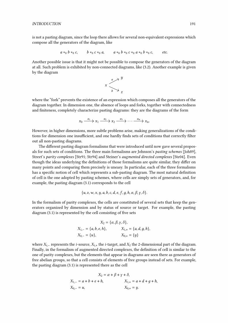
INTRODUCTION 191

is not a pasting diagram, since the loop there allows for several non-equivalent expressions whichcompose all the generators of the diagram, like

0 ∗0 1 ∗0 2, 1 ∗0 2 ∗0 0, 0 ∗0 1 ∗0 2 ∗0 0 ∗0 1 ∗0 2, etc.

Another possible issue is that it might not be possible to compose the generators of the diagramat all. Such problem is exhibited by non-connected diagrams, like (3.2). Another example is givenby the diagram

~

G

I

0

1

where the “fork” prevents the existence of an expression which composes all the generators of thediagram together. In dimension one, the absence of loops and forks, together with connectednessand �niteness, completely characterize pasting diagrams: they are the diagrams of the form

G0 G1 G2 · · · G=01 02 03 0= .

However, in higher dimensions, more subtle problems arise, making generalizations of the condi-tions for dimension one insu�cient, and one hardly �nds sets of conditions that correctly �lterout all non-pasting diagrams.

The di�erent pasting diagram formalisms that were introduced until now gave several propos-als for such sets of conditions. The three main formalisms are Johnson’s pasting schemes [Joh89],Street’s parity complexes [Str91; Str94] and Steiner’s augmented directed complexes [Ste04]. Eventhough the ideas underlying the de�nitions of those formalisms are quite similar, they di�er onmany points and comparing them precisely is uneasy. In particular, each of the three formalismshas a speci�c notion of cell which represents a sub-pasting diagram. The most natural de�nitionof cell is the one adopted by pasting schemes, where cells are simply sets of generators, and, forexample, the pasting diagram (3.1) corresponds to the cell

{D, E,F, G,~, 0, 1, 2, 3, 4, 5 , 6, ℎ, U, V,W, X}.

In the formalism of parity complexes, the cells are constituted of several sets that keep the gen-erators organized by dimension and by status of source or target. For example, the pastingdiagram (3.1) is represented by the cell consisting of �ve sets

-2 = {U, V,W, X},-1,− = {0, 1, 4, ℎ}, -1,+ = {0, 3, 6, ℎ},-0,− = {D}, -0,+ = {~}

where -8,− represents the 8-source, -8,+ the 8-target, and -2 the 2-dimensional part of the diagram.Finally, in the formalism of augmented directed complexes, the de�nition of cell is similar to theone of parity complexes, but the elements that appear in diagrams are seen there as generators offree abelian groups, so that a cell consists of elements of free groups instead of sets. For example,the pasting diagram (3.1) is represented there as the cell

-2 = U + V + W + X,-1,− = 0 + 1 + 4 + ℎ, -1,+ = 0 + 3 + 6 + ℎ,-0,− = D, -0,+ = ~.

192 CHAPTER 3. PASTING DIAGRAMS

The latter de�nition of cell, even though it is less natural at �rst, has the advantage of allowingthe use of tools from group theory and linear algebra in the proofs.

To the best of our knowledge, no formal account of the di�erences between the above threeformalisms was ever made. In particular, it was not known whether one of these formalisms ismore expressive than another. In this chapter, we carry out the task of formally relating them.It turns out that the three notions are incomparable in terms of expressive power (each of thethree allows a pasting diagram which is not allowed by others). In the process, it appearedthat the formalisms of parity complexes and pasting schemes are �awed, in the sense that thesets of conditions provided by the two formalisms are inadequate to �lter out all non-pastingdiagrams, refuting the related freeness properties of these structures claimed in the respectivearticles [Str91; Joh89]. We illustrate this problem by giving an example of a diagram which is nota pasting diagram but still accepted by both formalisms.

This motivated the introduction of a new formalism, called torsion-free complexes, whoseaxiomatic corrects and generalizes the one of parity complexes, and which are able to encompassaugmented directed complexes and �xed versions of parity complexes and pasting schemes. More-over, the good properties of their axiomatic allows for an e�cient computational implementationof torsion-free complexes, so that they can be used as part of a library for manipulating strictcategories.

We shall mention several recent works related to pasting diagrams and their formalisms.In [Buc15], Buckley gave a mechanized Coq proof of several results of [Str91] but stops beforehandling the freeness property of parity complexes, so that the de�ciency we point out in thischapter was missed. In [Cam16], Campbell isolates a common structure behind parity complexesand pasting schemes, called parity structure, and introduces another formalism with strongeraxioms than the ones of parity complexes and pasting schemes, taking an opposite path from thischapter where we introduce a more general formalism. In [Ngu17], Nguyen studies pre-polytopeswith labeled structures and shows that they induce a parity structure that satis�es a variant ofCampbell’s axioms that are enough to obtain another formalism for pasting diagrams.

Outline. This chapter is organized as follows. We �rst recall the de�nitions and the axioms ofeach of the existing formalisms: parity complexes (Section 3.1.2), pasting schemes (Section 3.1.3)and augmented directed complexes (Section 3.1.4). Then, by reusing the de�nitions used in paritycomplexes, we introduce the formalism of torsion-free complexes (Section 3.1.5). We providegeneral axioms for them (Paragraph 3.1.5.1) and also stronger ones that are more amenable tocomputations (Paragraph 3.1.5.5). We relate each of the four formalisms to the unifying notion ofl-hypergraph (Section 3.1.1), so that each formalism can be described as a class ofl-hypergraphs(the ones that satisfy the axioms of the formalism) together with a notion of cell (which representsa pasting diagram) and operations on these cells. We also discuss the counter-example to thefreeness property of parity complexes and pasting schemes (Paragraph 3.1.2.13).

Then, we prove that torsion-free complexes satisfy the properties expected from a pastingdiagram formalism. We �rst show that cells of a torsion-free complex have a structure of anl-category by adapting the results of Street [Str91] (Section 3.2, c.f. Theorem 3.2.3.3), and thenprove that this l-category is the free l-category on a canonical l-polygraph associated with thistorsion-free complex (Section 3.3, c.f. Corollary 3.3.3.5).

Next, we give other possible de�nitions of cells for torsion-free complexes (Section 3.4). Indeed,whereas we reused the de�nition of cells of parity complexes for torsion-free complexes, weshow that the l-category of cells can be equivalently obtained using other de�nitions for cells:maximal-well-formed sets (Theorem 3.4.1.24) and closed-well-formed sets (Theorem 3.4.1.27). Thelatter are similar to the cells of pasting schemes, and allow a more user-friendly approach oftorsion-free complexes. We illustrate this by providing an extension of cateq which enables

3.1. THE FORMALISMS OF PASTING DIAGRAMS 193

to specify cells of free categories on polygraphs using closed-well-formed sets of torsion-freecomplexes (Paragraph 3.4.1.32), after characterizing when a polygraph can be represented by atorsion-free complex (Theorem 3.4.1.29).

Finally, we relate the torsion-free complexes to the three other formalisms (Section 3.4). Weshow that the parity complexes, pasting schemes (after �xing their common de�ciency), andaugmented directed complexes are special cases of torsion-free complexes (Theorem 3.4.2.3, The-orem 3.4.3.9 and Theorem 3.4.4.22). Those are the only embeddings that exist between the fourformalisms and we provide counter-examples to the others (Section 3.4.5).

3.1 The formalisms of pasting diagrams

In this section, we introduce the de�nitions of the formalisms of pasting diagrams that we willconsider in this chapter. We present them through the common perspective of l-hypergraphs,that are structures which encode the information in diagrams of generators like (3.1). Then, thede�nition of each formalism roughly follows the same pattern. First, a de�nition for cells thatrepresent pasting diagrams is introduced, together with an identity and composition operationsthat aim at equipping those cells with a structure of l-category. Then, a class of l-hypergraphsthat are correctly handled by the considered formalism is de�ned by the mean of axioms orconditions.

We �rst introduce l-hypergraphs (Section 3.1.1) and then recall the de�nitions of the threemain existing formalisms for pasting diagrams: parity complexes (Section 3.1.2), pasting schemes(Section 3.1.3) and augmented directed complexes (Section 3.1.4). Then, we introduce the newformalism of torsion-free complexes that share the de�nitions of parity complexes but have di�erentaxioms on l-hypergraphs (Section 3.1.5).

3.1.1 Hypergraphs

In this section, we introduce the structure of l-hypergraph that we will use as a common basisin order to de�ne the pasting diagram formalisms. This notion is essentially the same as the oneof parity structure introduced by Campbell in [Cam16] when de�ning a new formalism whoseinstances are both parity complexes and pasting schemes. It is also similar to the notion oforiented graded poset that, in a related context, Hadzihasanovic used to de�ne presentations ofpolygraphs [Had18].

3.1.1.1 — De�nition. A graded set is a set % together with a partition

% =⊔=∈N

%=

the elements of %= being of dimension =. An l-hypergraph is a graded set % , the elements ofdimension = being called =-generators, together with, for = ∈ N and for each generator D ∈ %=+1,two �nite subsetsD−, D+ ⊆ %= called the source and target ofD. Given a subset* ⊆ % and n ∈ {−, +},we write* n for

* n =⋃D∈*

Dn .

Simple l-hypergraphs can be represented graphically using diagrams, where 0-generators arerepresented by their names, and higher generators by arrows→,⇒, V, etc. that represent re-spectively 1-generators, 2-generators, 3-generators etc.

194 CHAPTER 3. PASTING DIAGRAMS

Example 3.1.1.2. The diagram~

G ⇓ U I

~ ′

20

1 3

(3.3)

represents the l-hypergraph % with

%0 = {G,~,~ ′, I}, %1 = {0, 1, 2, 3}, %2 = {U},

and %= = ∅ for = ≥ 3, sources and targets being

0− = {G}, 0+ = {~}, U− = {0, 2}, U+ = {1, 3},

and so on.

3.1.1.3 — Fork-freeness. Given an l-hypergraph % and = ∈ N, a subset* ⊆ %= is fork-free (alsocalled well-formed in [Str91]) when:

– either = = 0 and |* | = 1,

– or = > 0 and for all D, E ∈ * and n ∈ {−, +}, we have Dn ∩ En = ∅.

For example, the subset {0, 1} of (3.3) is not fork-free since 0− ∩ 1− = {G}, but {0, 2} is.

Remark 3.1.1.4. Note that the de�nition of fork-freeness depends on the intended dimension =.This subtlety is important in the case of the empty set: ∅ is not well-formed as a subset of %0 butit is as a subset of %= when = > 0.

3.1.1.5 — The relation ⊳. Given an l-hypergraph % , = ∈ N∗ and * ⊆ %= , for D, E ∈ * , wewrite D ⊳1

*E when D+ ∩ E− ≠ ∅ and we de�ne the relation ⊳* on * as the transitive closure of ⊳1

*.

Given subsets+ ,, ⊆ * , we write+ ⊳*, when there existD ∈ + and E ∈, such thatD ⊳* E . Wede�ne the relation ⊳ on % by putting D ⊳ E when there exists = ∈ N∗ such that D, E ∈ %= and D ⊳%= E .The l-hypergraph % is then said acyclic when ⊳ is irre�exive.

Example 3.1.1.6. The l-hypergraph represented by

G ~

0

1

(3.4)

is not acyclic since 0 ⊳ 1 ⊳ 0. On the contrary, the l-hypergraph represented by (3.1) is acyclic.

Given a subset + ⊆ * , we say that + is a segment for ⊳* when for all D1, D2, D3 ∈ * such that

D1, D3 ∈ + and D1 ⊳* D2 ⊳* D3,

it holds that D2 ∈ + . For + ⊆ * , we say that + is initial (resp. terminal) in * when, for all D ∈ * ,if there exists E ∈ + such that D ⊳* E (resp. E ⊳* D), then D ∈ + .

Remark 3.1.1.7. In [Str91], ⊳ is de�ned as a transitive and re�exive relation whereas in [Joh89], itis only de�ned as a transitive relation. Here, we prefer the transitive (and not re�exive) de�nition,since it carries more information than the transitive and re�exive de�nition.

3.1. THE FORMALISMS OF PASTING DIAGRAMS 195

3.1.1.8 — Other source and target operations. Given an l-hypergraph % , for = ≥ 2, D ∈ %=and n, [ ∈ {−, +}, we write Dn[ for (Dn )[ . We extend the notation to subsets* ⊆ %= and write* n[for (* n )[ . Moreover, we write D∓ and D± for

D∓ = D− \ D+ and D± = D+ \ D−.

We also extend the notation to subsets* ⊆ %= and write* ∓ and* ± for

* ∓ = * − \* + and * ± = * + \* − .

Example 3.1.1.9. Consider the l-hypergraph represented by the diagram

F

E G

C D F ′ ~ I

E ′ G ′

F ′′

3

⇓ V2

2′′

⇓ U4

⇓ X0

1

1′

3′′

3′′′

⇓ W

5

2′′′

2′

4′

3′

. (3.5)

For this l-hypergraph, we have

U−− = {D, E}, U+− = {D, E ′}, U−∓ = {D}, U+± = {F ′}

and, writting* for the set {0, 1, 2, 3, 4, 5 },

* − = {C,D, E,F, G,~}, * + = {D, E,F, G,~, I},* ∓ = {C}, * ± = {I}

and, writting + for the set {U, V,W, X},

+ − = {1, 2, 2 ′′, 2 ′′′, 3, 3 ′′, 3 ′′′, 4}, + + = {1 ′, 2 ′, 2 ′′, 2 ′′′, 3 ′, 3 ′′, 3 ′′′, 4 ′},+ ∓ = {1, 2, 3, 4}, + ± = {1 ′, 2 ′, 3 ′, 4 ′}.

From the above examples, one can intuitively describe the operations (−)− and (−)+ as computingthe “inner” sources and targets of a set of generators, whereas the operations (−)∓ and (−)±compute the source and target “borders” of a set of generators.

3.1.2 Parity complexes

In this subsection, we recall the formalism of parity complexes developed by Street in [Str91].Most of the content will be reused when de�ning torsion-free complexes. The idea behind theformalism is to represent an (=+1)-cell as a pair of source and target =-cells together with a subsetof %=+1 which “moves” the source =-cell to the target =-cell. Under the axioms of parity complexes,these cells will have a structure of l-category.

196 CHAPTER 3. PASTING DIAGRAMS

3.1.2.1 — Pre-cells. Let % be an l-hypergraph. For = ∈ N, an =-pre-cell of % is a tuple

- = (-0,−, -0,+, . . . , -=−1,−, -=−1,+, -=)

of �nite subsets of % , such that -8,n ⊆ %8 for 8 ∈ N=−1 and n ∈ {−, +}, and -= ⊆ %= . By convention,we often denote -= by -=,− or -=,+. We write PCell(%) for the graded set of pre-cells of % .

Given = ∈ N, n ∈ {−, +} and an (=+1)-pre-cell - of % , we de�ne the =-pre-cell mn= (- ) as

mn= (- ) = (-0,−, -0,+, . . . , -=−1,−, -=−1,+, -=,n ) .

The globular conditions mn= ◦ m−=+1 = mn= ◦ m+=+1 are then trivially satis�ed, so that the functions m−, m+equip PCell(%) with a structure of an l-globular set.

3.1.2.2 — Movement and orthogonality. Let % be an l-hypergraph. Given = ∈ N and �nitesets

" ⊆ %=+1, * ⊆ %= and + ⊆ %= ,

we say that " moves * to + when

* = (+ ∪"−) \"+ and + = (* ∪"+) \"−.

Intuitively, the �rst equation means that* is the subset obtained from + by replacing the targetof " by its source, and the second equation has a dual meaning.

Example 3.1.2.3. In the l-hypergraph (3.5), the set {U, V,W, X} moves the set {0, 1, 2, 3, 4, 5 } to theset {0, 1 ′, 2 ′, 3 ′, 4 ′, 5 }.

3.1.2.4 — Cells. Let % be an l-hypergraph. Given = ∈ N, an =-cell of % is an =-pre-cell of % , suchthat

(i) -8+1,n moves -8,− to -8,+ for 8 ∈ N=−1 and n ∈ {−, +},

(ii) -8,n is fork-free for 8 ∈ N= and n ∈ {−, +}.

We denote by Cell(%) the graded set of cells of % , which inherits the structure of globular setfrom PCell(%). An =-cell - can be represented as on Figure 3.1 where each arrow

* +

"

means that " moves* to + .

Example 3.1.2.5. The l-hypergraph represented by (3.5) has, among others,

– a 0-cell ({C}),

– a 1-cell ({C}, {F ′}, {0, 1, 2 ′′}, {0, 1, 2 ′′′}, {U}),

– a 2-cell ({C}, {I}, {0, 1, 2, 3, 4, 5 }, {0, 1 ′, 2 ′, 3 ′, 4 ′, 5 }, {U, V,W, X}), etc.

Remark 3.1.2.6. In [Str91], cells are de�ned as pairs (", # ) with ", # ⊆ % satisfying conditionssimilar to the fork-freeness and movement conditions. This de�nition is equivalent to the aboveone: given an =-cell (in the sense of Street) (", # ), one obtains an =-cell - (in our sense), bysetting -= = "= and, for 8 ∈ N=−1, -8,− = "8 and -8,+ = #8 , and an inverse translation is de�nedeasily.

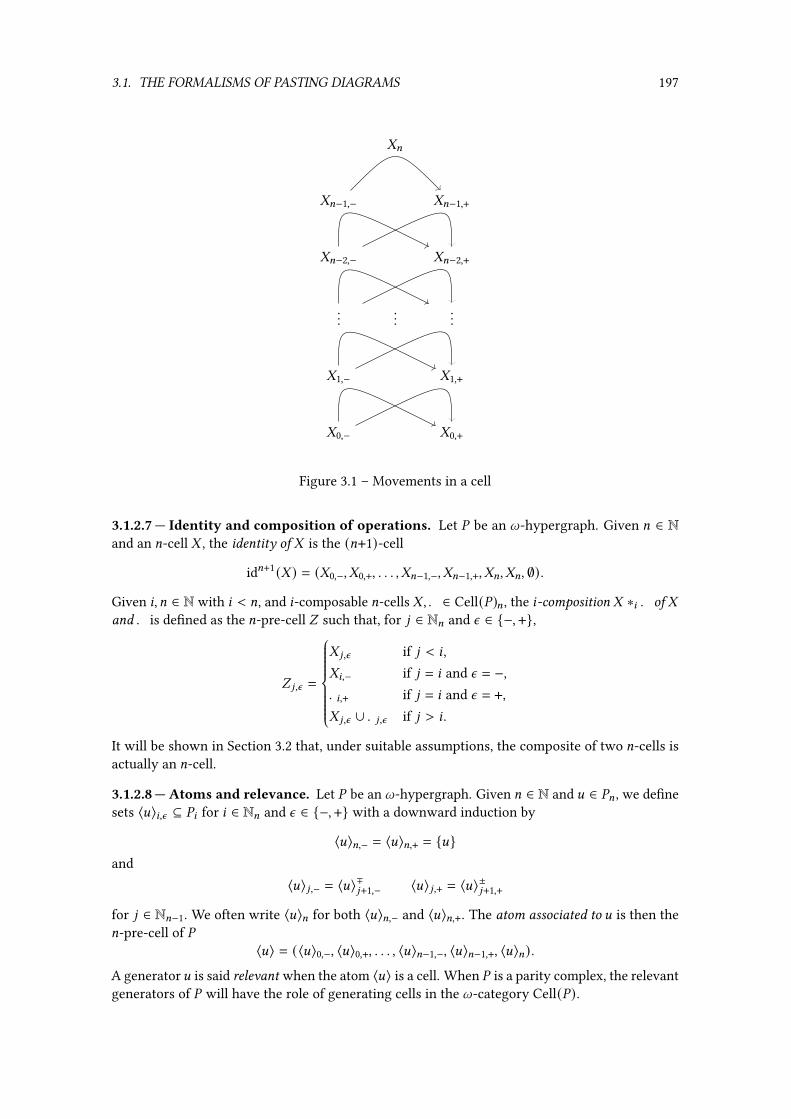
3.1. THE FORMALISMS OF PASTING DIAGRAMS 197

-=

-=−1,− -=−1,+

-=−2,− -=−2,+

......

...

-1,− -1,+

-0,− -0,+

Figure 3.1 – Movements in a cell

3.1.2.7 — Identity and composition of operations. Let % be an l-hypergraph. Given = ∈ Nand an =-cell - , the identity of - is the (=+1)-cell

id=+1(- ) = (-0,−, -0,+, . . . , -=−1,−, -=−1,+, -=, -=, ∅) .

Given 8, = ∈ N with 8 < =, and 8-composable =-cells -,. ∈ Cell(%)= , the 8-composition - ∗8 . of -and . is de�ned as the =-pre-cell / such that, for 9 ∈ N= and n ∈ {−, +},

/ 9,n =

- 9,n if 9 < 8 ,-8,− if 9 = 8 and n = −,.8,+ if 9 = 8 and n = +,- 9,n ∪ .9,n if 9 > 8 .

It will be shown in Section 3.2 that, under suitable assumptions, the composite of two =-cells isactually an =-cell.

3.1.2.8 — Atoms and relevance. Let % be an l-hypergraph. Given = ∈ N and D ∈ %= , we de�nesets 〈D〉8,n ⊆ %8 for 8 ∈ N= and n ∈ {−, +} with a downward induction by

〈D〉=,− = 〈D〉=,+ = {D}and

〈D〉9,− = 〈D〉∓9+1,− 〈D〉9,+ = 〈D〉±9+1,+for 9 ∈ N=−1. We often write 〈D〉= for both 〈D〉=,− and 〈D〉=,+. The atom associated to D is then the=-pre-cell of %

〈D〉 = (〈D〉0,−, 〈D〉0,+, . . . , 〈D〉=−1,−, 〈D〉=−1,+, 〈D〉=).A generatorD is said relevant when the atom 〈D〉 is a cell. When % is a parity complex, the relevantgenerators of % will have the role of generating cells in the l-category Cell(%).

198 CHAPTER 3. PASTING DIAGRAMS

Example 3.1.2.9. The atom associated to U in (3.3) is 〈U〉 with

〈U〉0,− = {D}, 〈U〉1,− = {0, 2}, 〈U〉2 = {U},〈U〉0,+ = {I}, 〈U〉1,+ = {1, 3},

and, since it is a cell, U is relevant.

3.1.2.10 — Tightness. Some defects were found in the �rst de�nition of parity complexes givenin [Str91], so that Street �xed his de�nition in [Str94]. His correction involves the notion oftightness de�ned as follows. Given = ∈ N, a subset* ⊆ %= is said to be tight when, for allD, E ∈ %=such that D ⊳ E and E ∈ * , we have D− ∩* ± = ∅.Example 3.1.2.11. In (3.5), * = {V,W} is not tight since U ⊳W and 2 ′′ ∈ U− ∩ * ±. Howeover, theset* ′ = {U, V,W, X} is tight.

3.1.2.12 — Parity complexes. We can now state the de�nition of a parity complex, reformulatingthe one given in [Str91] by taking into account the corrections introduced in [Str94]. A paritycomplex is an l-hypergraph % satisfying the axioms (C0) to (C5) below:

(C0) for = ∈ N∗ and D ∈ %= , D− ≠ ∅ and D+ ≠ ∅;

(C1) for = ∈ N with = ≥ 2 and D ∈ %= , D−− ∪ D++ = D−+ ∪ D+−;

(C2) for = ∈ N∗ and D ∈ %= , D− and D+ are fork-free;

(C3) % is acyclic;

(C4) for = ∈ N∗, D, E ∈ %= , F ∈ %=+1, if D ⊳ E , D ∈ Fn and E ∈ F[ for some n, [ ∈ {−, +},then n = [;

(C5) for 8, = ∈ N with 8 < = and D ∈ %= , 〈D〉8,− is tight.

Axiom (C0) ensures that each generator has de�ned source and target. Axiom (C1) enforces basicglobular properties on generators. For example, it forbids the l-hypergraph

F G ~ I

0

1

⇓ U (3.6)

since U−− ∪ U++ = {F,~} and U+− ∪ U−+ = {G, I}. Axiom (C2) forbids generators with parallelelements in their sources or targets. For example, the l-hypergraph

G

~I

0 (3.7)

does not satisfy Axiom (C2) since 0− = {G,~} is not fork-free. Axiom (C3) forbids l-hypergraphswith some loops like (3.4). Axiom (C4) can be informally described as forbidding “bridges”. Forinstance, the l-hypergraph

~

G ⇓ U I

~ ′

1

2

0

0′ 1′

(3.8)

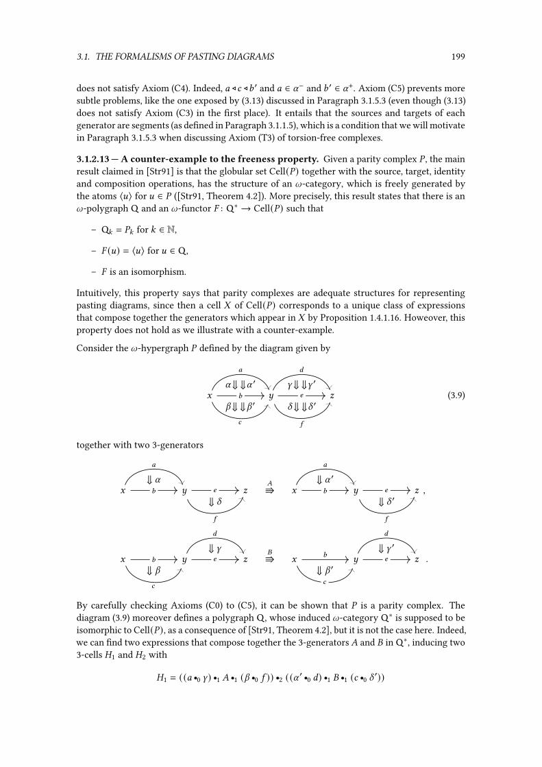
3.1. THE FORMALISMS OF PASTING DIAGRAMS 199

does not satisfy Axiom (C4). Indeed, 0 ⊳ 2 ⊳1 ′ and 0 ∈ U− and 1 ′ ∈ U+. Axiom (C5) prevents moresubtle problems, like the one exposed by (3.13) discussed in Paragraph 3.1.5.3 (even though (3.13)does not satisfy Axiom (C3) in the �rst place). It entails that the sources and targets of eachgenerator are segments (as de�ned in Paragraph 3.1.1.5), which is a condition that we will motivatein Paragraph 3.1.5.3 when discussing Axiom (T3) of torsion-free complexes.

3.1.2.13 — A counter-example to the freeness property. Given a parity complex % , the mainresult claimed in [Str91] is that the globular set Cell(%) together with the source, target, identityand composition operations, has the structure of an l-category, which is freely generated bythe atoms 〈D〉 for D ∈ % ([Str91, Theorem 4.2]). More precisely, this result states that there is anl-polygraph Q and an l-functor � : Q∗ → Cell(%) such that

– Q: = %: for : ∈ N,

– � (D) = 〈D〉 for D ∈ Q ,

– � is an isomorphism.

Intuitively, this property says that parity complexes are adequate structures for representingpasting diagrams, since then a cell - of Cell(%) corresponds to a unique class of expressionsthat compose together the generators which appear in - by Proposition 1.4.1.16. Howeover, thisproperty does not hold as we illustrate with a counter-example.

Consider the l-hypergraph % de�ned by the diagram given by

G ~ I1

0

2

U ⇓ ⇓U ′

V ⇓ ⇓V ′4

3

5

W ⇓ ⇓W ′

X ⇓ ⇓X ′(3.9)

together with two 3-generators

G ~ I1

0

⇓ U4

5

⇓ X

�V G ~ I1

0

⇓ U ′4

5

⇓ X ′,

G ~ I1

2

⇓ V4

3

⇓ W�V G ~ I

1

2

⇓ V ′4

3

⇓ W ′.

By carefully checking Axioms (C0) to (C5), it can be shown that % is a parity complex. Thediagram (3.9) moreover de�nes a polygraph Q , whose induced l-category Q∗ is supposed to beisomorphic to Cell(%), as a consequence of [Str91, Theorem 4.2], but it is not the case here. Indeed,we can �nd two expressions that compose together the 3-generators � and � in Q∗, inducing two3-cells �1 and �2 with

�1 = ((0 r0 W) r1 � r1 (V r0 5 )) r2 ((U ′ r0 3) r1 � r1 (2 r0 X ′))

200 CHAPTER 3. PASTING DIAGRAMS

and�2 = ((U r0 3) r1 � r1 (2 r0 X)) r2 ((0 r0 W ′) r1 � r1 (V ′ r0 5 ))

that share the same source and target

m−2 (�1) = m−2 (�2) = G ~ I1

0

2

⇓U

⇓V4

3

5

⇓W

⇓X

m+2 (�1) = m+2 (�2) = G ~ I1

0

2

⇓U ′

⇓V ′4

3

5

⇓W ′

⇓X ′.

Note that we used a precategorical syntax for �1 and �2 in order to avoid putting too many id3

so that we get more readable expressions. The canonical morphism � : Q∗ → Cell(%) maps �1and �2 to the same 3-cell - de�ned by:

-3 = {�, �},-2,− = {U, V,W, X}, -2,+ = {U ′, V ′, W ′, X ′},-1,− = {0, 3}, -1,+ = {2, 5 },-0,− = {G}, -0,− = {I}.

However, �1 and �2 are di�erent cells in Q∗. Let’s verify this fact with cateq (c.f. Section 2.4.4).First, we de�ne the polygraph Q and the cells �1 and �2 in cateq:

# x,y,z := gen *# a,b,c := gen x -> y# d,e,f := gen y -> z# alpha,alpha' := gen a -> b# beta,beta' := gen b -> c# gamma,gamma' := gen d -> e# delta,delta' := gen e -> f# A := gen alpha *0 delta -> alpha' *0 delta'# B := gen beta *0 gamma -> beta' *0 gamma'# H1 := ((id3 a *0 id3 gamma) *1 A *1 (id3 beta *0 id3 f))

*2 ((id3 alpha' *0 id3 d) *1 B *1 (id3 c *0 id3 delta'))# H2 := ((id3 alpha *0 id3 d) *1 B *1 (id3 c *0 id3 delta))

*2 ((id3 a *0 id3 gamma') *1 A *1 (id3 beta' *0 id3 f))

We then query whether �1 is equal to �2 with the command

# H1 = H2

to which cateq answers false , so that �1 ≠ �2 by Proposition 2.4.2.14 (before cateq wasimplemented, a proof in Agda that �1 ≠ �2 was given in [FM19]).

Hence, the distinct cells �1 and �2 of Q∗ are sent to the same cell of Cell(%) by � as onecould have expected, since the information that makes�1 and�2 di�erent is the order in which�

3.1. THE FORMALISMS OF PASTING DIAGRAMS 201

and � are composed, which can not be expressed by a cell of a parity complex. This refutes [Str91,Theorem 4.2] which asserts that � is an isomorphism. Thus, parity complexes do not necessarilyinduce free l-categories in general.

3.1.3 Pasting schemes

Johnson’s loop-free pasting schemes [Joh89] is another proposed formalism for pasting diagrams.Like parity complexes, they are based on l-hypergraphs, but the cells will now be representedas single subsets of generators instead of tuples like for parity complexes (which is arguably amore natural representation of pasting diagrams compared to the cells of parity complexes). Asa consequence, one will rely on set relations, namely B and E, on the l-hypergraph to de�nethe globular operations on the cells. Concretely, B and E encode which generators to remove toobtain respectively the target and the source of a cell. We introduce the formalism in detail below.

3.1.3.1 — Conventions for relations. First, we set some elementary de�nitions and notationsfor relations. A relation between two sets - and . is a subset L ⊆ - × . . For (G,~) ∈ - × . ,we write G L~ when (G,~) ∈ L. The identity relation on a set - is the relation L ⊆ - × - suchthat G L~ i� G = ~. Given a binary relation L between - and . , and G ∈ - , we write L(G) for theset

L(G) = {~ ∈ . | G L~}.

More generally, given a subset - ′ ⊆ - , we denote by L(- ′) the set

{~ ∈ . | ∃G ∈ - ′, G L~}.

The relation L is said �nitary when, for all G ∈ - , L(G) is a �nite set. If L is a relation on agraded set % = t=∈N%= , given :, ; ∈ N, we write L;

:for the relation between %; and %: de�ned

as L∩(%; × %: ). Similarly, we write L; for the relation between %; and % de�ned as L∩(%; × %).Given relations L between - and . and L′ between . and / , we write LL′ for the relation

between - and / which is the composite relation de�ned as

LL′ = {(G, I) ∈ - × / | ∃~ ∈ ., G L~ and ~ L′ I}.

3.1.3.2 — Pre-pasting schemes. A pre-pasting scheme (%,B, E) is given by a graded set % andtwo relations B, E (for “beginning” and “end”) on % such that

(i) B and E are �nitary,

(ii) for :, ; ∈ N with ; < : , B;:= E;

:= ∅,

(iii) B::

(resp. E::) is the identity relation on %: ,

(iv) for :, ; ∈ N with : < ; , L ∈ {B, E}, D ∈ %;+1 and E ∈ %: , D L;+1:E if and only if

D L;+1;

B;:E and D L;+1

;E;:E .

Example 3.1.3.3. The diagram (3.3) can be encoded as a pre-pasting scheme

B21(U) = {0, 2}, E2

1(U) = {1, 3},B2

0(U) = {~}, E20(U) = {~ ′},

B10(0) = {G}, E1

0(0) = {~} . . .

202 CHAPTER 3. PASTING DIAGRAMS

Note that the relations B and E of a pre-pasting scheme % are completely determined by the dataof B:+1

:(D) and E:+1

:(D) for : ∈ N and D ∈ %: . As a consequence, the data of a pre-pasting scheme

structure on % is equivalent to the data of an l-hypergraph structure on % : the correspondenceis given by

D− = B:+1:(D) and D+ = E:+1

:(D)

for : ∈ N∗ and D ∈ %:+1. In particular, the relation ⊳ on a pasting scheme is de�ned as the one onthe associated l-hypergraph.

3.1.3.4 — Direct loops. Given an l-hypergraph % , % has a direct loop when

(i) either there exist = ∈ N∗ and D, E ∈ %= such that D ⊳ E and E(E) ∩ B(D) ≠ ∅,

(ii) or there existsF ∈ % such that E(F) ∩ B(F) ≠ {F}.

Example 3.1.3.5. The l-hypergraph

~

G I

~

02

1

01

21 22

⇓ U

⇓ V(3.10)

has a direct loop by the �rst criterion, because U ⊳ V and ~ ∈ B(U) ∩ E(V). Examples of directloops by the second condition are given by the l-hypergraphs

%1 = E F

0

0

⇓ U and %2 =

~

G ⇓ V I

~

21

1′ 2′

. (3.11)

Indeed, in %1, we have 0 ∈ B(U) ∩ E(U), and, in %2, we have ~ ∈ B(V) ∩ E(V).

3.1.3.6 — Finite graded subsets. Let % be a pre-pasting scheme. We de�ne the relation R ⊆ %×%as the smallest re�exive transitive relation on % such that, for all : ∈ N and G ∈ %:+1, we have

B(G) ∪ E(G) ⊆ R(G).

Example 3.1.3.7. In the case of the l-hypergraph (3.10), we have

R(U) = {G,~, I, 01, 02, 1, U} and R(V) = {G,~, I, 1, 21, 22, V}.

A �nite graded subset of dimension = of % (abbreviated =-fgs) is an (=+1)-tuple - = (-0, . . . , -=)such that -: ⊆ %: and -: is �nite for : ∈ N= . We often identify the =-fgs - with the set ∪:∈N=-: ,but one should keep in mind that the =-fgs - and the (=+1)-fgs (-0, . . . , -=, ∅) are two di�erentobjects. We say that - is closed when R(- ) = - . Given = ∈ N and an (=+1)-fgs - of % , we de�nethe source and the target of - as the =-fgs’s m−= (- ) and m+= (- ) of % such that

m−= (- ) = - \ E= (- ) and m+= (- ) = - \ B= (. ) .

Example 3.1.3.8. Considering the l-hypergraph (3.10), we have

m−= (R(U)) = R(U) \ {1, U} = {G,~, I, 01, 02} and m+= (R(U)) = R(U) \ {~, 01, 02} = {G, I, 1}.

Remark 3.1.3.9. The fgs’s of the form R(D) for D ∈ % are the analogue of the atoms de�ned forparity complexes.

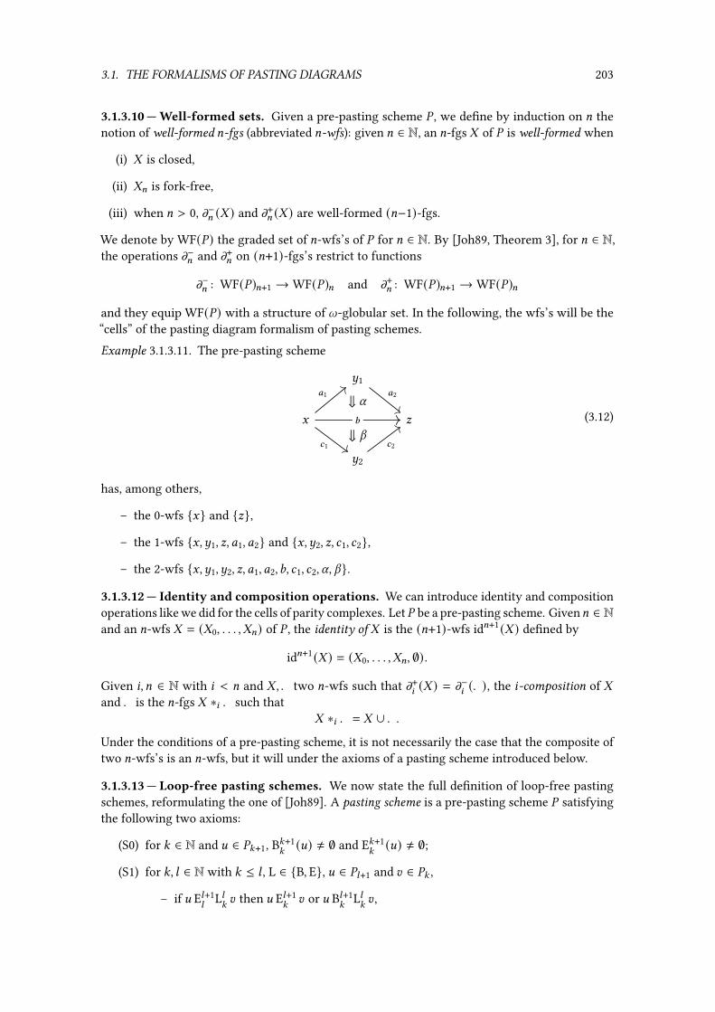
3.1. THE FORMALISMS OF PASTING DIAGRAMS 203

3.1.3.10 —Well-formed sets. Given a pre-pasting scheme % , we de�ne by induction on = thenotion of well-formed =-fgs (abbreviated =-wfs): given = ∈ N, an =-fgs - of % is well-formed when

(i) - is closed,

(ii) -= is fork-free,

(iii) when = > 0, m−= (- ) and m+= (- ) are well-formed (=−1)-fgs.

We denote by WF(%) the graded set of =-wfs’s of % for = ∈ N. By [Joh89, Theorem 3], for = ∈ N,the operations m−= and m+= on (=+1)-fgs’s restrict to functions

m−= : WF(%)=+1 →WF(%)= and m+= : WF(%)=+1 →WF(%)=

and they equip WF(%) with a structure of l-globular set. In the following, the wfs’s will be the“cells” of the pasting diagram formalism of pasting schemes.Example 3.1.3.11. The pre-pasting scheme

~1

G I

~2

02

1

01

21 22

⇓ U

⇓ V(3.12)

has, among others,

– the 0-wfs {G} and {I},

– the 1-wfs {G,~1, I, 01, 02} and {G,~2, I, 21, 22},

– the 2-wfs {G,~1, ~2, I, 01, 02, 1, 21, 22, U, V}.

3.1.3.12 — Identity and composition operations. We can introduce identity and compositionoperations like we did for the cells of parity complexes. Let % be a pre-pasting scheme. Given= ∈ Nand an =-wfs - = (-0, . . . , -=) of % , the identity of - is the (=+1)-wfs id=+1(- ) de�ned by

id=+1(- ) = (-0, . . . , -=, ∅) .

Given 8, = ∈ N with 8 < = and -,. two =-wfs such that m+8 (- ) = m−8 (. ), the 8-composition of -and . is the =-fgs - ∗8 . such that

- ∗8 . = - ∪ . .

Under the conditions of a pre-pasting scheme, it is not necessarily the case that the composite oftwo =-wfs’s is an =-wfs, but it will under the axioms of a pasting scheme introduced below.

3.1.3.13 — Loop-free pasting schemes. We now state the full de�nition of loop-free pastingschemes, reformulating the one of [Joh89]. A pasting scheme is a pre-pasting scheme % satisfyingthe following two axioms:

(S0) for : ∈ N and D ∈ %:+1, B:+1:(D) ≠ ∅ and E:+1

:(D) ≠ ∅;

(S1) for :, ; ∈ N with : ≤ ; , L ∈ {B, E}, D ∈ %;+1 and E ∈ %: ,

– if D E;+1;

L;:E then D E;+1

:E or D B;+1

:L;:E ,

204 CHAPTER 3. PASTING DIAGRAMS

– if D B;+1;

L;:E then D B;+1

:E or D E;+1

;L;:E .

The pasting scheme % is a loop-free pasting scheme when it moreover satis�es the followingaxioms:

(S2) % has no direct loops;

(S3) for D ∈ % , R(D) ∈ WF(%);

(S4) for :, = ∈ N with : < =, - ∈ WF(%): and D ∈ %= ,

– if m−:(R(D)) ⊆ - , then 〈D〉:,− is a segment for ⊳-: ,

– if m+:(R(D)) ⊆ - , then 〈D〉:,+ is a segment for ⊳-: ;

(S5) for = ∈ N, - ∈ WF(%)= and D ∈ %=+1 with m−= (R(D)) ⊆ - , the following hold:

(a) - ∩ E(D) = ∅,(b) for ~ ∈ - , if B(D) ∩ R(~) ≠ ∅, then ~ ∈ B(D).

Axiom (S1) enforces basic globular properties on generators and forbids, for example, thel-hyper-graph (3.6). Axiom (S2) forbids l-hypergraphs with loops like (3.4), (3.10) and (3.11). Axiom (S3)enforces fork-freeness on the iterated sources and targets of a generator (for example, it forbids thel-hypergraph (3.7)). Axiom (S4) relates to Axiom (C5) of parity complexes and prevent situationsin the spirit of (3.13) discussed in Paragraph 3.1.5.3 (even though (3.13) does not satisfy Axiom (S2)in the �rst place). We motivate this axiom in Paragraph 3.1.5.3 when we discuss a similar axiom fortorsion-free complexes. Axiom (S5) can be deduced from the other axioms (c.f. [Joh87, Theorem3.7]) but it simpli�es the proofs of [Joh89]. An example of a sensible pre-pasting scheme thatsatisfy Axioms (S0) to (S3), but neither Axiom (S4) nor Axiom (S5), exists in dimension four(see [Pow91, Example 3.11]).

3.1.3.14 — A counter-example to the freeness property. The main result claimed in [Joh89] issimilar to the one of [Str91]: given a loop-free pasting scheme % , the globular set WF(%) togetherwith the source, target, identity and composition operations has the structure of an l-category,which is freely generated by the wfs’s R(D) for D ∈ % ([Joh89, Theorem 13]), i.e., there exist anl-polygraph Q and an l-functor � : Q∗ →WF(%) such that

– Q: = %: for : ∈ N,

– � (D) = R(D) for D ∈ Q ,

– � is an isomorphism.

But the same �aw as for parity complexes is present here too, which makes the freeness resultwrong. In fact, the counter-example to the freeness property of parity complexes, introduced inParagraph 3.1.2.13, is also a counter-example to the freeness property of pasting schemes: thel-hypergraph % is a loop-free pasting scheme and the canonical morphism � : Q∗ → WF(%)sends �1 and �2 to the same 3-wfs - where

- = {G,~, I, U, V,W, X, U ′, V ′, W ′, X ′, �, �}

refuting the freeness property [Joh89, Theorem 13].

3.1. THE FORMALISMS OF PASTING DIAGRAMS 205

3.1.4 Augmented directed complexes

Augmented directed complexes, designed by Steiner in [Ste04], are not directly based on l-hyper-graphs, but on chain complexes. Under the conditions required by Steiner, it happens that thedata of a chain complex is equivalent to the data of an l-hypergraph. The de�nition of cells forthis formalism strongly resembles the one of parity complexes. The only di�erence is that thecells are tuples of group elements instead of subsets of an l-hypergraph. We recall the formalismin detail below.

3.1.4.1 — Augmented directed complex. A pre-augmented directed complexes ( , d, e) (abbre-viated pre-adc) is the data of

– for = ∈ N, an abelian group = together with a distinguished submonoid ∗= ⊆ = ,

– for = ∈ N, group morphisms called boundary operators

d= : =+1 → =,

– an augmentation, that is, a group morphism

e : 0 → Z.

An augmented directed complex, abbreviated adc, is a pre-adc ( , d, e) such that

e ◦ d0 = 0 and d= ◦ d=+1 = 0 for = ∈ N.

3.1.4.2 — Bases for pre-adc’s. Given a pre-adc ( , d, e), a basis of ( , d, e) is the data of a gradedset % ⊆ ⊔

=∈N = such that each ∗= is the free commutative monoid on %= and each = is the freeabelian group on ∗= . Given a basis % of ( , d, e), every element D ∈ = can be uniquely written as

D =∑6∈%=

D66,

with D6 ∈ Z such that D6 ≠ 0 for a �nite number of 6 ∈ %= . This representation induces a partialorder ≤ where, for = ∈ N and D, E ∈ = , D ≤ E when D6 ≤ E6 for all 6 ∈ %= . Given = ∈ Nand D, E ∈ = we can de�ne a greatest lower bound D ∧ E of D and E by

D ∧ E =∑6∈%=

min(D6, E6)6.

Given = ∈ N and D ∈ =+1, we write D∓, D± ∈ ∗= for the unique elements satisfying

d= (D) = D± − D∓ and D∓ ∧ D± = 0.

Moreover, we write D−, D+ for

D− =∑6∈%=+1

D66∓ and D+ =

∑6∈%=+1

D66±.

Remark 3.1.4.3. The elements D∓ and D± are respectively denoted by m−(D) and m+(D) in [Ste04].We adopt the former notation for consistency with those of Section 3.1.2.

206 CHAPTER 3. PASTING DIAGRAMS

3.1.4.4 — From 8-hypergraphs to pre-adc’s with basis. Given an l-hypergraph % , we de�nethe pre-adc ( , d, e) associated to % as follows. For = ∈ N, ∗= is de�ned as the free commutativemonoid on %= and = as the free abelian group on ∗= . The augmentation e : 0 → Z is de�ned asthe unique morphism such that e(G) = 1 for G ∈ %0. Given = ∈ N and a �nite subset * ⊆ %= , wewrite Σ= (* ) for

∑D∈* D ∈ = . Then, d= : =+1 → = is de�ned as the unique morphism such that

d= (D) = Σ= (D+) − Σ= (D−)

for D ∈ %=+1. Then, canonically admits % as a basis. We say that % is an adc when is an adc.Example 3.1.4.5. We explicitly describe the pre-adc associated to the l-hypergraph (3.12) asfollows. Writting (∗ for the free commutative monoid on a set ( , we put

∗0 = {G,~1, ~2, I}∗, ∗1 = {01, 02, 1, 21, 22}∗, ∗2 = {U, V}∗

and ∗= = {0} for = ≥ 3. 0, 1, 2 and = for = ≥ 3 are then the induced free abelian groupson these monoids. The operations e and d are de�ned by universal property to be the uniquemorphisms such that

e(G) = e(~1) = e(~2) = e(I) = 1and

d0(01) = ~1 − G , d0(02) = I − ~1, d0(1) = I − G ,d0(21) = ~2 − G , d0(22) = I − ~2,d1(U) = 1 − (01 + 02), d1(V) = (21 + 22) − 1.

We can now give some examples for the operations (−)∓ and (−)± operations de�ned above:

(01 + 02)∓ = G, (01 + 02)± = I,(U + V)∓ = 01 + 02, (U + V)± = 21 + 22.

We moreover illustrate the operations (−)− and (−)+:

(01 + 02)− = G + ~1 (01 + 02)+ = ~1 + I(U + V)− = 01 + 02 + 1 (U + V)+ = 1 + 21 + 22.

Thus, the operations (−)∓ and (−)± compute the source and target “borders” of an element of = ,whereas the operations (−)− and (−)+ compute the sum of the “inner” sources and targets ofan element of = . They are the analogues of the operations de�ned for l-hypergraph in Para-graph 3.1.1.8.

3.1.4.6 — Cells. Let be a pre-adc. Given = ∈ N, an =-pre-cell of is given by an (2=+1)-tuple

- = (-0,−, -0,+, . . . , -=−1,−, -=−1,+, -=)

with -= ∈ ∗= and -8,−, -8,+ ∈ ∗8 for 8 ∈ N=−1. For the sake of conciseness, we often referto -= by -=,− or -=,+. We write PCell∗( ) for the graded set of pre-cells of . When = > 0,given n ∈ {−, +}, we de�ne the =-pre-cell mn= (- ) as

mn= (- ) = (-0,−, -0,+, . . . , -=−1,−, -=−1,+, -=,n ) .

The globular conditions mn= ◦ m−=+1 = mn= ◦ m+=+1 are then trivially satis�ed and the functions m−, m+equip PCell∗( ) with a structure of l-globular set.

Given = ∈ N, an =-cell of is an =-pre-cell - of such that

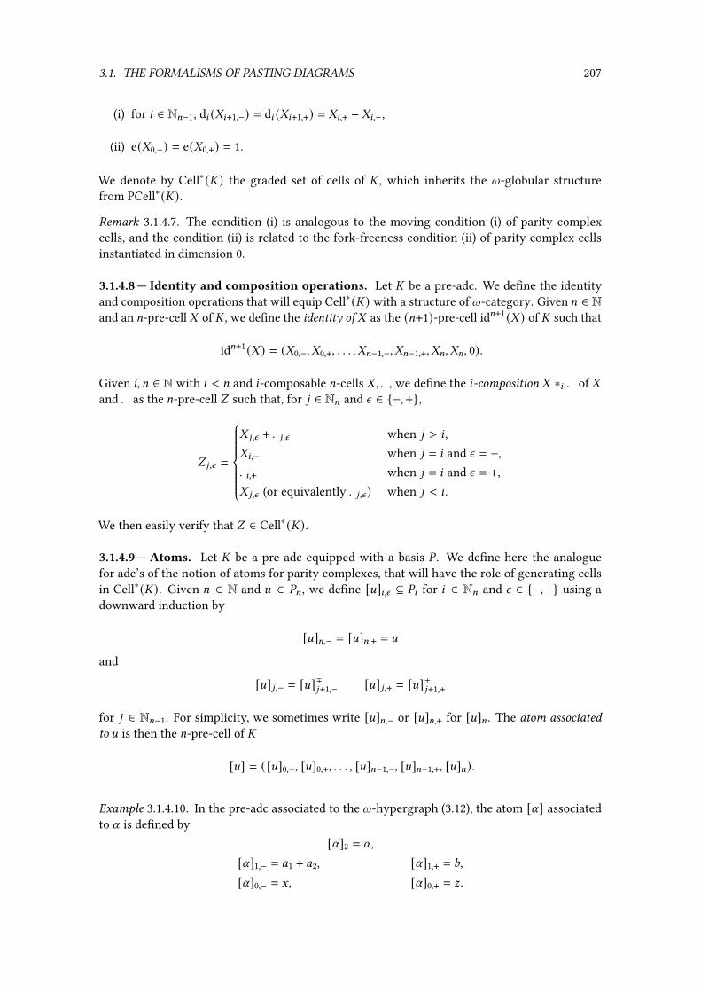
3.1. THE FORMALISMS OF PASTING DIAGRAMS 207

(i) for 8 ∈ N=−1, d8 (-8+1,−) = d8 (-8+1,+) = -8,+ − -8,−,

(ii) e(-0,−) = e(-0,+) = 1.

We denote by Cell∗( ) the graded set of cells of , which inherits the l-globular structurefrom PCell∗( ).

Remark 3.1.4.7. The condition (i) is analogous to the moving condition (i) of parity complexcells, and the condition (ii) is related to the fork-freeness condition (ii) of parity complex cellsinstantiated in dimension 0.

3.1.4.8 — Identity and composition operations. Let be a pre-adc. We de�ne the identityand composition operations that will equip Cell∗( ) with a structure of l-category. Given = ∈ Nand an =-pre-cell - of , we de�ne the identity of - as the (=+1)-pre-cell id=+1(- ) of such that

id=+1(- ) = (-0,−, -0,+, . . . , -=−1,−, -=−1,+, -=, -=, 0).

Given 8, = ∈ N with 8 < = and 8-composable =-cells -,. , we de�ne the 8-composition - ∗8 . of -and . as the =-pre-cell / such that, for 9 ∈ N= and n ∈ {−, +},

/ 9,n =

- 9,n + .9,n when 9 > 8 ,-8,− when 9 = 8 and n = −,.8,+ when 9 = 8 and n = +,- 9,n (or equivalently .9,n ) when 9 < 8 .

We then easily verify that / ∈ Cell∗( ).

3.1.4.9 — Atoms. Let be a pre-adc equipped with a basis % . We de�ne here the analoguefor adc’s of the notion of atoms for parity complexes, that will have the role of generating cellsin Cell∗( ). Given = ∈ N and D ∈ %= , we de�ne [D]8,n ⊆ %8 for 8 ∈ N= and n ∈ {−, +} using adownward induction by

[D]=,− = [D]=,+ = D

and

[D]9,− = [D]∓9+1,− [D]9,+ = [D]±9+1,+

for 9 ∈ N=−1. For simplicity, we sometimes write [D]=,− or [D]=,+ for [D]= . The atom associatedto D is then the =-pre-cell of

[D] = ( [D]0,−, [D]0,+, . . . , [D]=−1,−, [D]=−1,+, [D]=).

Example 3.1.4.10. In the pre-adc associated to the l-hypergraph (3.12), the atom [U] associatedto U is de�ned by

[U]2 = U,[U]1,− = 01 + 02, [U]1,+ = 1,[U]0,− = G, [U]0,+ = I.

208 CHAPTER 3. PASTING DIAGRAMS

3.1.4.11 — Unital loop-free basis. Let be a pre-adc equipped with a basis �. Given 8 ∈ N, wede�ne a relation <8 on � as the smallest transitive relation such that, for :, ; ∈ Nwith 8 < min(:, ;),and D ∈ �: , E ∈ �; with [D]8,+ ∧ [E]8,− ≠ 0, we have D <8 E . The basis � is then said

– unital when for all D ∈ �, e( [D]0,−) = e( [D]0,+) = 1,

– loop-free when, for all 8 ∈ N, <8 is irre�exive.

Example 3.1.4.12. Consider the pre-adc with basis � derived from the hypergraph (3.4). Thebasis � is then unital but not loop-free since 0 <0 1 <0 0. Now, consider the pre-adc with basis �derived from the hypergraph (3.7). The basis � is then not unital since e( [0]0,−) = e(G + ~) = 2,but it is loop-free. Now consider the pre-adc with basis � derived from the hypergraph (3.5).We have, among others, the relations

0 <0 1 <0 2 <0 3 <0 4 <0 5 ,0 <0 U <0 X <0 5 ,

V <1 U <1 W and V <1 X <1 W .

It can be veri�ed that � is unital and loop-free.

3.1.4.13 — The freeness property. In [Ste04], the author shows that, given an adc with a loop-free unital basis �, the globular set Cell∗( ), together with identity and composition operations,has a structure of an l-category which is freely generated by the atoms [D] for D ∈ �, i.e., thereexist an l-polygraph Q and an l-functor � : Q∗ → Cell∗( ) such that

– Q: = �: for : ∈ N,

– � (D) = [D] for D ∈ Q ,

– � is an isomorphism.

Contrary to parity complexes and pasting schemes, the pre-adc with basis associated to thel-hypergraph (3.9) is not a loop-free adc. Indeed, it is an adc with unital basis, but the basisis not loop-free since � <1 � <1 �. Thus, augmented directed complexes are, to the best ofour knowledge, the only formalism of pasting diagrams among the three that we have alreadyintroduced for which the freeness property holds.

3.1.5 Torsion-free complexes

In this section, we introduce torsion-free complexes. They are a new formalism for pasting diagramsbased on parity complexes. More precisely, torsion-free complexes rely on the same notion of cellthan parity complexes, but satisfy di�erent axioms, namely the axioms (T0) to (T4) introduced inParagraph 3.1.5.1. Whereas the axioms (T0) to (T2) were already present in [Str91], Axiom (T3)generalizes Axiom (C4) and Axiom (C5) of parity complexes, and can be thought as an equivalentof Axiom (S4) of pasting schemes. Axiom (T4) prevents diagrams with “torsion” as exhibited bythe counter-example to the freeness property provided for parity complexes and pasting schemes(c.f. Paragraph 3.1.2.13). Under these new axioms, the category of cells (as de�ned in Section 3.1.2)is freely generated by the atoms, as proved in Section 3.3. The proofs will be the object of thefollowing sections.

3.1. THE FORMALISMS OF PASTING DIAGRAMS 209

3.1.5.1 — De�nitions. Here, we give the axiomatics of torsion-free complexes, after giving aconcise reformulation of Axiom (S4), and introducing the notion of torsion, the consideration ofwhich solves the issue of parity complexes and pasting schemes illustrated by the example givenin Paragraph 3.1.2.13.

Let % be an l-hypergraph. Given : ∈ N and D ∈ %: , we say that D satis�es the segmentcondition when, for all = ∈ N:−1 and every =-cell- such that 〈D〉=,− ⊆ -= , it holds that both 〈D〉=,−and 〈D〉=,+ are segments for ⊳-= .

Given =, :, ; ∈ N with 0 < = < min(:, ;), D ∈ %: , E ∈ %; and an =-cell - , D and E are said to bein torsion with respect to - when

〈D〉=,+ ⊆ -=, 〈E〉=,− ⊆ -=, 〈D〉=,+ ∩ 〈E〉=,− = ∅ and 〈D〉=,+ ⊳-= 〈E〉=,− ⊳-= 〈D〉=,+.

We will give some intuition on these de�nitions in the following paragraphs after we gave thede�nition of torsion-free complexes. The l-hypergraph % is then a torsion-free complex when itsatis�es the following axioms:

(T0) (non-emptiness) for all D ∈ % , D− ≠ ∅ and D+ ≠ ∅;

(T1) (acyclicity) % is acyclic;

(T2) (relevance) for all D ∈ % , D is relevant;

(T3) (segment condition) for D ∈ % , D satis�es the segment condition;

(T4) (torsion-freeness) for all =, :, ; ∈ N∗ with = < min(:, ;), D ∈ %: , E ∈ %; and every=-cell - , D and E are not in torsion with respect to - .

We shall now give some intuition about these axioms.

3.1.5.2 — Axioms (T1) and (T2). Axiom (T1) enforces the same notion of acyclicity than forparity complexes, forbidding loops like

G ⇓ U ~

5

5

andG ~

I

5

6ℎ.

Axiom (T2) requires that the generators of the l-hypergraph induce cells, forbidding l-hyper-graphs like (3.6) and (3.7). It can be shown that Axiom (T2) entails Axioms (C1) and (C2) of paritycomplexes.

3.1.5.3 — The segment Axiom (T3). Recall that our goal is to �nd conditions on l-hyper-graphs P so that the l-category of cells Cell(%) is freely generated by the atoms. In particular,every cell should be decomposable as a composite of context classes applied to atoms (c.f. Propo-sition 2.2.5.3). But there are cells of l-hypergraphs satisfying Axioms (T0) to (T2) that can notbe decomposed this way. The problem comes from an incompatibility between two concurrentphenomena:

(i) on the one side, the decomposition property that we want requires that some orders ofcompositions be allowed;

(ii) on the other side, the relation ⊳ imposes restrictions on the orders in which the generatorscan be composed.

210 CHAPTER 3. PASTING DIAGRAMS

I

~

G

F

3 ′

3

0′02

1

1 ′

4

U1⇒⇒U ′1

U4⇒⇒U ′4

U2⇒

U3⇐

I

~

G

3 ′3

0′0 U1⇒

U4⇒�V

I

~

G

3 ′3

0′0 U ′1⇒

U ′4⇒(3.13)

Figure 3.2 – A problematic l-hypergraph

We illustrate this incompatibility in an example. Consider the l-hypergraph % represented onFigure 3.2 where, more precisely,

�− = {U1, U4}, �+ = {U ′1, U ′4},U−1 = U ′1

−= {0}, U+1 = U ′1

+= {0′},

U−4 = U ′4−= {3}, U+4 = U ′4

+= {3 ′}, etc.

One can verify that % satis�es Axioms (T0), (T1) and (T2). In thisl-hypergraph, there is a 2-cell-given by

-2 = {U1, U2, U3, U4},-1,− = {0, 1}, -1,+ = {2, 3 ′, 4},-0,− = {G}, -0,+ = {I},

and a 3-cell . given by

.3 = {�},.2,− = {U1, U2, U3, U4}, .2,+ = {U1, U

′2, U′3, U4},

.1,− = {0, 1}, .1,+ = {2, 3 ′, 4},

.0,− = {G}, .0,+ = {I}

so that - = m−2 (. ). Suppose by contradiction that Cell(%) is an l-category which is freelygenerated by the atoms. Then, by the decomposition property of cells of free extensions (Propo-sition 2.2.5.3), and by the value of .3, . can be written

. = �1 [〈�〉] ∗2 · · · ∗2 �: [〈�〉]

for some 2-context classes �1, . . . , �: of type 〈�〉 (it can moreover be shown that : = 1 but it isnot important at the moment). Since - = m−2 (. ), it implies that - can be written

- = q ∗1 - ′ ∗1 k (3.14)

where - ′ = id25∗0 m−2 (〈�〉) ∗0 id2

6 for some 2-cells q,k and 1-cells 5 , 6 in Cell(%), illustrating (i).Since Cell(%)≤2 ' Cell(% \ {�})≤2 and % \ {�} is a torsion-free complex, using Lemma 3.2.3.1introduced later, the existence of the composite (3.14) implies that

the sets q2, - ′2 andk2 form a partition of -2 = {U1, U2, U3, U4}, (3.15)

3.1. THE FORMALISMS OF PASTING DIAGRAMS 211

and, using Lemma 3.3.3.3 introduced later, that

for (V,W) ∈ (q2 × (- ′2 ∪k2)) ∪ ((k2 ∪ - ′2) ×k2), we have ¬(W ⊳-2 V), (3.16)

or, more simply put, the partition q2, -′2,k2 respects the relation ⊳-2 , illustrating (ii). We show

that (3.15) and (3.16) entails a contradiction. Consider U2 ∈ -2. Since we have

- ′2 = �− = {U1, U4},

by (3.15), either U2 ∈ q2 or U2 ∈ k2. By (3.16), since U1 ⊳1-2U2, we have U2 ∈ k2. Now con-

sider U3 ∈ -2. By (3.15), either U3 ∈ q2 or U3 ∈ k2. By (3.16), since U3 ⊳1-2U4, we have U3 ∈ q2. But

then,U3 ∈ q2, U2 ∈ k2 and U2 ⊳

1-2U3,

contradicting (3.16). Hence, Cell(%) is not an l-category freely generated by the atoms.

Axiom (T3) prevents this kind of problems and, in particular, forbids the l-hypergraph % . Indeed,we have

〈�〉2,− = {U1, U4} ⊆ -2, U1 ⊳-2 U2 ⊳-2 U3 ⊳-2 U4 and U2, U3 ∉ 〈�〉2,−so that 〈�〉2,− is not a segment for ⊳-2 , and � does not satisfy the segment condition.

3.1.5.4 — The torsion-freeness Axiom (T4). The notion of torsion captures the essence of thecounter-example to the freeness property of parity complexes and pasting schemes presentedin Paragraph 3.1.2.13. Indeed, considering the l-hypergraph % represented by (3.9), there is a2-cell - de�ned by

-2 = {U ′, V, W, X ′},-1,− = {0, 3}, -1,+ = {2, 5 },-0,− = {G}, -0,+ = {I},

which is induced by the pasting diagram

G ~ I1

0

2

⇓U ′

⇓V4

3

5

⇓W

⇓X ′.

Then, one can verify that � and � are in torsion with respect to - , so that % does not satisfyAxiom (T4) (on the other hand, it satis�es Axioms (T0) to (T3)).

Intuitively, the situations with torsion are the minimal cases where the freeness property failsfor a parity complex % (and similarly for a pasting scheme % ). When D, E ∈ % are in torsion withrespect to a cell - of % , there are two possible order to compose D and E : �rst D then E , or �rst Ethen D. And both composites produce equal cells in Cell(%). However, this equality can not bededuced from an exchange law, since the torsion says basically that D and E cross each other,preventing to obtain the left-hand side of Axiom (S-vi) of l-categories (c.f. Paragraph 1.4.1.1).

3.1.5.5 — More computable axioms. Axioms (T3) and (T4) happen to be hard to check in prac-tice. Indeed, both involve a quanti�cation on all the cells of an l-hypergraph, and enumeratingthem can be tough since their number is exponential in the number of elements of the l-hyper-graph in the worst case. Here, we give stronger axioms that are simpler to verify, in the sensethat they can be checked using an algorithm with polynomial complexity.

212 CHAPTER 3. PASTING DIAGRAMS

Given an l-hypergraph % , for = ∈ N, D, E ∈ %= , we write D y E when there exists F ∈ %=+1such that D ∈ F− and E ∈ F+ and we write y∗ for the re�exive transitive closure of y.For * ,+ ⊆ %= , we write * y∗ + when there exist D ∈ * and E ∈ + such that D y∗ E .Consider the following axiom on an l-hypergraph % :

(T3’) for :, = ∈ N∗ with : < = and D ∈ %= , we do not have 〈D〉:,+ y∗ 〈D〉:,−.

Then, Axiom (T3) can be replaced by Axiom (T3’) in the axioms of torsion-free complexes:

Lemma 3.1.5.6. Let % be an l-hypergraph satisfying Axioms (T0), (T1) and (T2). If % satis�esAxiom (T3’), then it satis�es Axiom (T3).

Proof. Suppose that % satis�es Axiom (T3’). Let=, : ∈ Nwith= < : ,- be an=-cell andD ∈ %: suchthat 〈D〉=,− ⊆ -= . If = = 0, there is nothing to prove, so we can assume = > 0. By contradiction,suppose that 〈D〉=,− is not a segment for ⊳-= . So there are A ∈ N with A > 2 and D1, . . . , DA ∈ -=such that

D1, DA ∈ 〈D〉=,−, D2, . . . , DA−1 ∉ 〈D〉=,− and D8 ⊳1-=D8+1

for 8 ∈ N∗A−1. In particular, there are E1, . . . , EA−1 ∈ %=−1 such that E8 ∈ D+8 ∩ D−8+1 for 8 ∈ N∗A−1.GivenF ∈ -= such that E1 ∈ F−, since -= is fork-free, we haveF = D2 ∉ 〈D〉=,−. Thus, since D isrelevant by Axiom (T2), E1 ∈ 〈D〉±=,− = 〈D〉=−1,+. Similarly, EA−1 ∈ 〈D〉=−1,−. So 〈D〉=−1,+ y∗ 〈D〉=−1,−,contradicting Axiom (T3’). Hence, % satis�es Axiom (T3). �

Now, consider the following axiom on an l-hypergraph % :

(T4’) for =, :, ; ∈ N∗ with = < min(:, ;), D ∈ %: and E ∈ %; , if 〈D〉=,+ ∩ 〈E〉=,− = ∅, then atmost one of the following holds:

– 〈D〉=−1,+ y∗ 〈E〉=−1,−,

– 〈E〉=−1,+ y∗ 〈D〉=−1,−.

Then, Axiom (T4) can be replaced by Axiom (T4’) in the axioms of torsion-free complexes:

Lemma 3.1.5.7. Let % be an l-hypergraph satisfying Axioms (T0), (T1) and (T2). If % satis�esAxiom (T4’), then it satis�es Axiom (T4).

Proof. Suppose that % satis�es Axiom (T4’). By contradiction, assume that % does not satisfyAxiom (T4). So there are =, :, ; ∈ N∗ with = < min(:, ;), D ∈ %: , E ∈ %; and an =-cell - such that Dand E are in torsion with respect to - . That is,

〈D〉=,+ ⊆ -=, 〈E〉=,− ⊆ -=, 〈D〉=,+ ∩ 〈E〉=,− = ∅ and 〈D〉=,+ ⊳-= 〈E〉=,− ⊳-= 〈D〉=,+.

By the last condition, there are A ∈ N with A > 1, andF1, . . . ,FA ∈ -= such that

F1 ∈ 〈D〉=,+, FA ∈ 〈E〉=,−, F2, . . . ,FA−1 ∉ 〈D〉=,+ ∪ 〈E〉=,−, and F8 ⊳1-=F8+1

for 8 ∈ N∗A−1. Thus, there are F1, . . . , FA−1 ∈ %=−1 such that F8 ∈ F+8 ∩ F−8+1 for 8 ∈ N∗A−1.GivenF ∈ -= with F1 ∈ F−, we haveF = F2 ∉ 〈D〉=,+ since -= is fork-free. Thus,

F1 ∈ 〈D〉±=,+ = 〈D〉=−1,+.

Similarly, FA−1 ∈ 〈E〉=−1,−, so 〈D〉=−1,+ y∗ 〈E〉=−1,−. Likewise, we have 〈E〉=−1,+ y∗ 〈D〉=−1,−, whichcontradicts Axiom (T4’). Hence, % satis�es Axiom (T4). �

3.2. THE CATEGORY OF CELLS 213

3.2 The category of cells

In this section, we show that, given a torsion-free complex % ,the l-globular set Cell(%) has astructure of an l-category. Indeed, even though we de�ned identity and composition operationsin Paragraph 3.1.2.7, we do not know for now that the composition of two cells is a cell. Inorder to show this, we adapt the proofs of [Str91] and take the opportunity to simplify them. Inparticular, we give a detailed proof of the “gluing theorem” (Theorem 3.2.2.3, adapted from [Str91,Lemma 3.2]), which enables to build an (=+1)-cell from an =-cell by gluing a set of (=+1)-gene-rators.

3.2.1 Movement properties

Before being able to show the gluing theorem, we need some technical results about movement(notion which appears in the de�nition of cells). We state and prove here several such properties,some of which coming from [Str91].

In the following, we suppose given an l-hypergraph % . We �rst state a criterion for movement:

Lemma 3.2.1.1 ([Str91, Proposition 2.1]). For = ∈ N, �nite subsets * ⊆ %= and ( ⊆ %=+1, thereexists + ⊆ %= such that ( moves* to + if and only if (∓ ⊆ * and* ∩ (+ = ∅.

Proof. If ( moves* to + , then, by de�nition,

(∓ ⊆ (+ ∪ (−) \ (+ = *

and* ∩ (+ = ((+ ∪ (−) \ (+) ∩ (+ = ∅.

Conversely, if (∓ ⊆ * and* ∩ (+ = ∅, let + = (* ∪ (+) \ (−. Then

(+ ∪ (−) \ (+ = (* ∪ (+ ∪ (−) \ (+

= (* \ (+) ∪ ((− \ (+)= * ∪ (∓ (since* ∩ (+ = ∅)= * (since (∓ ⊆ * )

and ( moves* to + . �

The next property states that it is possible to modify a movement by adding or removing “inde-pendent” elements.

Lemma 3.2.1.2 ([Str91, Proposition 2.2]). Let = ∈ N,* ,+ ⊆ %= and ( ⊆ %=+1 be �nite subsets suchthat ( moves* to + . Then, given -,. ⊆ %= such that

- ⊆ * , - ∩ (∓ = ∅ and . ∩ ((− ∪ (+) = ∅,

we have that ( moves (* ∪ . ) \ - to (+ ∪ . ) \ - .

Proof. By Lemma 3.2.1.1, we have (∓ ⊆ * and * ∩ (+ = ∅. Using the hypothesis, we can re�neboth equalities to

(∓ ⊆ (* ∪ . ) \ - and ((* ∪ . ) \ - ) ∩ (+ = ∅.

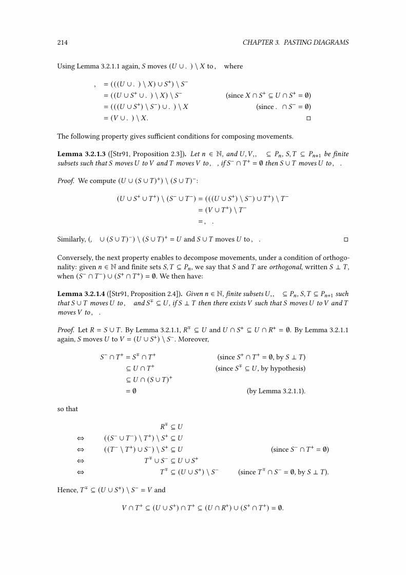
214 CHAPTER 3. PASTING DIAGRAMS

Using Lemma 3.2.1.1 again, ( moves (* ∪ . ) \ - to, where

, = (((* ∪ . ) \ - ) ∪ (+) \ (−

= ((* ∪ (+ ∪ . ) \ - ) \ (− (since - ∩ (+ ⊆ * ∩ (+ = ∅)= (((* ∪ (+) \ (−) ∪ . ) \ - (since . ∩ (− = ∅)= (+ ∪ . ) \ - . �

The following property gives su�cient conditions for composing movements.

Lemma 3.2.1.3 ([Str91, Proposition 2.3]). Let = ∈ N, and * ,+ ,, ⊆ %= , (,) ⊆ %=+1 be �nitesubsets such that ( moves* to + and ) moves + to, , if (− ∩) + = ∅ then ( ∪) moves* to, .

Proof. We compute (* ∪ (( ∪) )+) \ (( ∪) )−:

(* ∪ (+ ∪) +) \ ((− ∪) −) = (((* ∪ (+) \ (−) ∪) +) \) −

= (+ ∪) +) \) −

=, .

Similarly, (, ∪ (( ∪) )−) \ (( ∪) )+ = * and ( ∪) moves* to, . �

Conversely, the next property enables to decompose movements, under a condition of orthogo-nality: given = ∈ N and �nite sets (,) ⊆ %= , we say that ( and ) are orthogonal, written ( ⊥ ) ,when ((− ∩) −) ∪ ((+ ∩) +) = ∅. We then have:

Lemma 3.2.1.4 ([Str91, Proposition 2.4]). Given = ∈ N, �nite subsets* ,, ⊆ %= , (,) ⊆ %=+1 suchthat ( ∪) moves* to, and (∓ ⊆ * , if ( ⊥ ) then there exists + such that ( moves* to + and )moves + to, .

Proof. Let ' = ( ∪ ) . By Lemma 3.2.1.1, '∓ ⊆ * and * ∩ (+ ⊆ * ∩ '+ = ∅. By Lemma 3.2.1.1again, ( moves* to + = (* ∪ (+) \ (−. Moreover,

(− ∩) + = (∓ ∩) + (since (+ ∩) + = ∅, by ( ⊥ ) )⊆ * ∩) + (since (∓ ⊆ * , by hypothesis)⊆ * ∩ (( ∪) )+

= ∅ (by Lemma 3.2.1.1).

so that

'∓ ⊆ *⇔ (((− ∪) −) \) +) \ (+ ⊆ *⇔ (() − \) +) ∪ (−) \ (+ ⊆ * (since (− ∩) + = ∅)⇔ ) ∓ ∪ (− ⊆ * ∪ (+

⇔ ) ∓ ⊆ (* ∪ (+) \ (− (since ) ∓ ∩ (− = ∅, by ( ⊥ ) ).

Hence, ) ∓ ⊆ (* ∪ (+) \ (− = + and

+ ∩) + ⊆ (* ∪ (+) ∩) + ⊆ (* ∩ '+) ∪ ((+ ∩) +) = ∅.

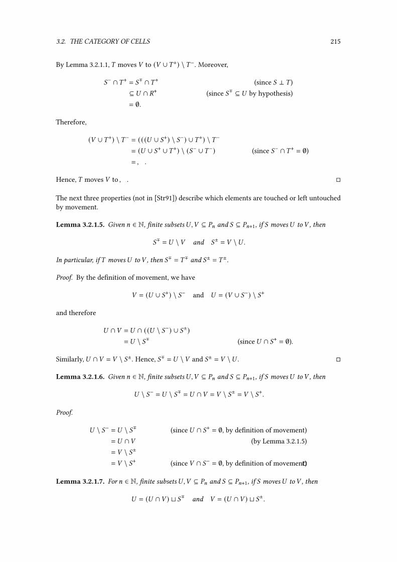
3.2. THE CATEGORY OF CELLS 215

By Lemma 3.2.1.1, ) moves + to (+ ∪) +) \) −. Moreover,

(− ∩) + = (∓ ∩) + (since ( ⊥ ) )⊆ * ∩ '+ (since (∓ ⊆ * by hypothesis)= ∅.

Therefore,

(+ ∪) +) \) − = (((* ∪ (+) \ (−) ∪) +) \) −

= (* ∪ (+ ∪) +) \ ((− ∪) −) (since (− ∩) + = ∅)=, .

Hence, ) moves + to, . �

The next three properties (not in [Str91]) describe which elements are touched or left untouchedby movement.

Lemma 3.2.1.5. Given = ∈ N, �nite subsets* ,+ ⊆ %= and ( ⊆ %=+1, if ( moves* to + , then

(∓ = * \+ and (± = + \* .

In particular, if ) moves* to + , then (∓ = ) ∓ and (± = ) ±.

Proof. By the de�nition of movement, we have

+ = (* ∪ (+) \ (− and * = (+ ∪ (−) \ (+

and therefore

* ∩+ = * ∩ ((* \ (−) ∪ (±)= * \ (∓ (since* ∩ (+ = ∅).

Similarly,* ∩+ = + \ (±. Hence, (∓ = * \+ and (± = + \* . �

Lemma 3.2.1.6. Given = ∈ N, �nite subsets* ,+ ⊆ %= and ( ⊆ %=+1, if ( moves* to + , then

* \ (− = * \ (∓ = * ∩+ = + \ (± = + \ (+.

Proof.

* \ (− = * \ (∓ (since* ∩ (+ = ∅, by de�nition of movement)= * ∩+ (by Lemma 3.2.1.5)= + \ (±

= + \ (+ (since + ∩ (− = ∅, by de�nition of movement)�

Lemma 3.2.1.7. For = ∈ N, �nite subsets* ,+ ⊆ %= and ( ⊆ %=+1, if ( moves* to + , then

* = (* ∩+ ) t (∓ and + = (* ∩+ ) t (±.

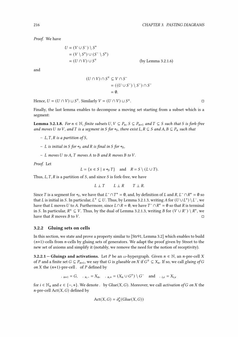
216 CHAPTER 3. PASTING DIAGRAMS

Proof. We have

* = (+ ∪ (−) \ (+

= (+ \ (+) ∪ ((− \ (+)= (* ∩+ ) ∪ (∓ (by Lemma 3.2.1.6)

and

(* ∩+ ) ∩ (∓ ⊆ + ∩ (−

= ((* ∪ (−) \ (−) ∩ (−

= ∅.

Hence,* = (* ∩+ ) t (∓. Similarly + = (* ∩+ ) t (±. �

Finally, the last lemma enables to decompose a moving set starting from a subset which is asegment:

Lemma 3.2.1.8. For = ∈ N, �nite subsets * ,+ ⊆ %= , ( ⊆ %=+1 and ) ⊆ ( such that ( is fork-freeand moves* to + , and ) is a segment in ( for ⊳( , there exist !, ' ⊆ ( and �, � ⊆ %= such that

– !,) , ' is a partition of ( ,

– ! is initial in ( for ⊳( and ' is �nal in ( for ⊳( ,

– ! moves* to �, ) moves � to � and ' moves � to + .

Proof. Let! = {G ∈ ( | G ⊳( ) } and ' = ( \ (! ∪) ).

Thus, !,) , ' is a partition of ( , and since ( is fork-free, we have

! ⊥ ) ! ⊥ ' ) ⊥ '.

Since) is a segment for ⊳( , we have that !−∩) + = ∅, and, by de�nition of ! and ', !−∩'+ = ∅ sothat ! is initial in ( . In particular, !∓ ⊆ * . Thus, by Lemma 3.2.1.3, writing� for (* ∪!+) \!−, wehave that ! moves* to�. Furthermore, since !∩' = ∅, we have) −∩'+ = ∅ so that ' is terminalin ( . In particular, '± ⊆ + . Thus, by the dual of Lemma 3.2.1.3, writing � for (+ ∪ '−) \ '+, wehave that ' moves � to + . �

3.2.2 Gluing sets on cells

In this section, we state and prove a property similar to [Str91, Lemma 3.2] which enables to build(=+1)-cells from =-cells by gluing sets of generators. We adapt the proof given by Street to thenew set of axioms and simplify it (notably, we remove the need for the notion of receptivity).

3.2.2.1 — Gluings and activations. Let % be an l-hypergraph. Given = ∈ N, an =-pre-cell -of % and a �nite set� ⊆ %=+1, we say that� is glueable on - if�∓ ⊆ -= . If so, we call gluing of�on - the (=+1)-pre-cell . of % de�ned by

.=+1 = �, .=,− = -=, .=,+ = (-= ∪�+) \�− and .8,n = -8,n

for 8 ∈ N= and n ∈ {−, +}. We denote . by Glue(-,�). Moreover, we call activation of� on - the=-pre-cell Act(-,�) de�ned by

Act(-,�) = m+= (Glue(-,�))

3.2. THE CATEGORY OF CELLS 217

�

-= (-= ∪�+) \�−

-=−1,− -=−1,+

...

-1,− -1,+

-0,− -0,+

- Act(-,�)

Glue(-,�)

Figure 3.3 – Cells involved and their movements in Theorem 3.2.2.3

We say that� is dually gluable on- when�± ⊆ -= and we de�ne the dual gluing Glue(-,�) andthe dual activation Act(-,�) in a similar fashion. For example, consider the l-hypergraph (3.13)from Paragraph 3.1.5.3 and recall there the de�nitions of - and . . Then {�} is glueable on -and Glue(-, {�}) = . , and Act(-, {�}) is the 2-pre-cell - with

-2 = {U1, U′2, U′3, U4},

-1,− = {0, 1}, -1,+ = {2, 3 ′, 4},-0,− = {G}, -0,+ = {I}.

Conversely, {�} is dually gluable on - , and we have Glue(- , {�}) = . , and Act(- , {�}) = - .

3.2.2.2 — The gluing theorem. We now prove the “gluing theorem”. It is an adaptation of [Str91,Lemma 3.2] which enables to build new cells using the gluing and activation operations. Thetheorem moreover gives additional results concerning intersections with the source and thetarget sets of gluing sets, that will have as consequence that the composition in the category ofcell Cell(%) respects the relation ⊳ (see Proposition 3.3.1.10).

Theorem 3.2.2.3. Let % be an l-hypergraph which satis�es Axioms (T0), (T1), (T2) and (T3).Given = ∈ N, an =-cell - of % and a �nite fork-free set � ⊆ %=+1 such that � is glueable on - , wehave that

(a) Act(-,�) is a cell and �+ ∩ -= = ∅,

(b) Glue(-,�) is a cell,

(c) given a �nite, fork-free subset � ′ ⊆ %=+1 which is dually glueable on - , � ′− ∩�+ = ∅.

and dual properties hold when � is dually gluable on - .

Proof. See Figure 3.3 for a representation of the cells in the statement of the theorem. In thefollowing, write ( for

( = Act(-,�)= = (-= ∪�+) \�−.

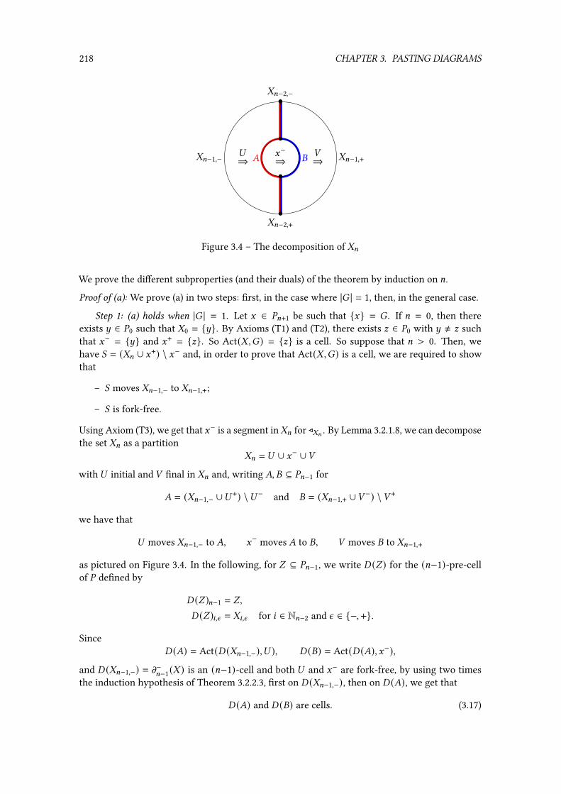
218 CHAPTER 3. PASTING DIAGRAMS

� �

•

•

•

•

-=−1,− -=−1,+

-=−2,−

-=−2,+

G−⇒

*⇒

+⇒

Figure 3.4 – The decomposition of -=

We prove the di�erent subproperties (and their duals) of the theorem by induction on =.

Proof of (a): We prove (a) in two steps: �rst, in the case where |� | = 1, then, in the general case.

Step 1: (a) holds when |� | = 1. Let G ∈ %=+1 be such that {G} = � . If = = 0, then thereexists ~ ∈ %0 such that -0 = {~}. By Axioms (T1) and (T2), there exists I ∈ %0 with ~ ≠ I suchthat G− = {~} and G+ = {I}. So Act(-,�) = {I} is a cell. So suppose that = > 0. Then, wehave ( = (-= ∪ G+) \ G− and, in order to prove that Act(-,�) is a cell, we are required to showthat

– ( moves -=−1,− to -=−1,+;

– ( is fork-free.

Using Axiom (T3), we get that G− is a segment in-= for ⊳-= . By Lemma 3.2.1.8, we can decomposethe set -= as a partition

-= = * ∪ G− ∪+

with* initial and + �nal in -= and, writing �, � ⊆ %=−1 for

� = (-=−1,− ∪* +) \* − and � = (-=−1,+ ∪+ −) \+ +

we have that

* moves -=−1,− to �, G− moves � to �, + moves � to -=−1,+

as pictured on Figure 3.4. In the following, for / ⊆ %=−1, we write � (/ ) for the (=−1)-pre-cellof % de�ned by

� (/ )=−1 = /,

� (/ )8,n = -8,n for 8 ∈ N=−2 and n ∈ {−, +}.

Since� (�) = Act(� (-=−1,−),* ), � (�) = Act(� (�), G−),

and � (-=−1,−) = m−=−1(- ) is an (=−1)-cell and both * and G− are fork-free, by using two timesthe induction hypothesis of Theorem 3.2.2.3, �rst on � (-=−1,−), then on � (�), we get that

� (�) and � (�) are cells. (3.17)

3.2. THE CATEGORY OF CELLS 219

By Axiom (T2), we have thatG+ is fork-free. (3.18)

Since G− moves � to �, by Lemma 3.2.1.1, we get

� ∩ G−+ = ∅. (3.19)

By Axiom (T2), it holds that G+∓ = G−∓ ⊆ �. By (3.17) and (3.18), using the induction hypothesisof Theorem 3.2.2.3 on � (�), we get

� ∩ G++ = ∅. (3.20)By Lemma 3.2.1.1, there exists �′ such that G+ moves � to �′, and

�′ = (� ∪ G++) \ G+−

= (� \ G+−) ∪ (G++ \ G+−)= (� \ G+∓) ∪ G+± (by (3.20))= (� \ G−∓) ∪ G−± (since G+∓ = G−∓, by Axiom (T2))= (� \ G−−) ∪ (G−+ \ G−−) (by (3.19))= (� ∪ G−+) \ G−−

= � (since G− moves � to �).

Hence,G+ moves � to �. (3.21)

Since G+∓ ⊆ � (�)=−1 and* ± ⊆ � (�)=−1, using the induction hypothesis of Theorem 3.2.2.3, by (c)we get

* − ∩ G++ = ∅. (3.22)Similarly, with � (�), we get

G+− ∩+ + = ∅. (3.23)By de�nition,* moves-=−1,− to�, andG+moves� to� by (3.21). Moreover, by (3.22),* −∩G++ = ∅.Using Lemma 3.2.1.3, we deduce that

* ∪ G+ moves -=−1,− to �. (3.24)

Since* and + are disjoint and respectively initial and terminal in -= , we have that* − ∩+ + = ∅.Also, by (3.23), we have (G+− ∩+ +) = ∅, therefore

(* ∪ G+)− ∩+ + ⊆ (* − ∩+ +) ∪ (G+− ∩+ +)= ∅.

Using (3.24) and Lemma 3.2.1.3, knowing that ( = * ∪ G+ ∪+ , we deduce that

( moves -=−1,− to -=−1,+. (3.25)

The set * ∪+ is fork-free as a subset of the fork-free -= , and G+ is fork-free since G is relevantby Axiom (T2). Moreover,

* − ∩ G+− = * − ∩ G+∓ (by (3.22))⊆ * − ∩� (by (3.21) and Lemma 3.2.1.1)= ∅ (since* moves -=−1,− to �),

* + ∩ G++ = * ± ∩ G++ (by (3.22))⊆ � ∩ G++ (by Lemma 3.2.1.1 since* moves -=−1,− to �)= ∅ (by (3.21) and Lemma 3.2.1.1).

220 CHAPTER 3. PASTING DIAGRAMS

So* ⊥ G+. Similarly, G+ ⊥ + . Hence, since ( = * ∪ G+ ∪+ ,

( is fork-free. (3.26)

Then, by (3.25) and (3.26),Act(-,�) is a cell.

Finally, we prove the second part of (a). By Axiom (T1), G− ∩ G+ = ∅ . Since * ⊥ G+ and G+ ⊥ +(by (3.26)), using Axiom (T0), we deduce that

* ∩ G+ = G+ ∩+ = ∅

so that-= ∩ G+ = (* ∪ G− ∪+ ) ∩ G+ = ∅

which concludes the proof of the Step 1.

Step 2: (a) holds. We prove this by induction on |� |. If |� | = 0, then the result is trivial.Moreover, the case |� | = 1 was proved in Step 1. So suppose that |� | ≥ 2. Since the relation ⊳ isacyclic by Axiom (T1), we can consider a minimal G ∈ � for ⊳� . Let

� = � \ {G}, * = (-= ∪ G+) \ G−, + = (* ∪ �+) \ �−

and recall that we de�ned ( as (-= ∪�+) \�−. In order to show that Act(-,�) is a cell, we arerequired to prove that:

– ( moves -=−1,− to -=−1,+;

– ( is fork-free.

For this purpose, we will �rst move -= with {G} to* and use Step 1, then move* by � to+ anduse the induction of Step 2. Finally, we will prove that+ = ( . So, using Step 1 with - and {G}, weget that

– Act(-, {G}) is a cell;

– in particular,* is fork-free and, when = > 0,* moves -=−1,− to -=−1,+;

– -= ∩ G+ = ∅.

By Lemma 3.2.1.1, we deduce that {G } moves -= to* . Moreover,

�∓ = �− \ �+

= (�− \ G−) \ (�+ \ G+) (since fork-freeness implies that �n = tD∈�Dn )⊆ ((�− \ G−) \�+) ∪ G+

= ((�− \�+) \ G−) ∪ G+

⊆ (-= \ G−) ∪ G+ (since �∓ ⊆ -= by Lemma 3.2.1.1)⊆ (-= ∪ G+) \ G− (since G− ∩ G+ = ∅ by Axiom (T1))= * .

Also, � is fork-free as a subset of the fork-free set � . Using the induction hypothesis of Step 2for � , we get that

– Act(Act(-, {G}), �) is a cell;

3.2. THE CATEGORY OF CELLS 221

– In particular, + = (* ∪ �+) \ �− is fork-free, and, when = > 0, + moves -=−1,− to -=−1,+;

– * ∩ �+ = ∅.

By Lemma 3.2.1.1, we deduce that � moves * to + . Also, note that G− ∩ �+ = ∅ since Gwas taken minimal in � . Using Lemma 3.2.1.3, we deduce that � = {G} ∪ � moves -= to + .But ( = (-= ∪�+) \�− so that ( = + .

The second part of (a) is left to show, that is, -= ∩�+ = ∅. We compute that

-= ∩�+ = (* ∪ G− \ G+) ∩�+ (by Lemma 3.2.1.1, since {G } moves -= to* )= ((* ∪ G−) ∩�+) \ G+

= (* ∩�+) \ G+ (since G− ∩� = G− ∩ (G+ ∪ �) = ∅)= (* ∩ �+)= ∅

which concludes the proofs of Step 2 and (a).

Proof of (b): By (a), Act(-,�) is a cell. To conclude, we need to show that � moves -= to ( . Byde�nition of ( , we have that ( = (-= ∪�+) \�−. Moreover,

(( ∪�−) \�+ = (((-= ∪�+) \�−) ∪�−) \�+

= (-= ∪�+ ∪�−) \�+

= (-= \�+) ∪�∓

= -= ∪�∓ (since -= ∩�+ = ∅ by (a))= -= (since � is glueable on - ).

Hence, Glue(-,�) is a cell.

Proof of (c): By contradiction, suppose that � ′− ∩ �+ ≠ ∅. Then, there are G ∈ � ′, ~ ∈ �and I ∈ G− ∩ ~+. Consider

* = {G ′ ∈ � ′ | G ⊳�′ G ′} ∪ {G},+ = {~ ′ ∈ � | ~ ′ ⊳� ~} ∪ {~}.

By the acyclicity Axiom (T1), we have

* + ∩+ − = ∅.

Since* is a terminal set for ⊳�′ , we have in particular* + ∩� ′− ⊆ * −. So,

* + = (* + \� ′−) ∪ (* + ∩� ′−) ⊆ � ′± ∪* −.

Hence, * ± ⊆ � ′± ⊆ -= (since � ′ is dually glueable on - ). Similarly, + ∓ ⊆ -= . Using thedual version of (a), the =-pre-cell . = Act(-,* ) is an =-cell such that .= = (-= ∪* −) \* + (seeFigure 3.5) and we have

+ ∓ = + ∓ \* + (since + − ∩* + = ∅)⊆ -= \* + (since + ∓ ⊆ -=)⊆ (-= ∪* −) \* +

= .= .

222 CHAPTER 3. PASTING DIAGRAMS

-=

I~⇒

I G⇒

� ′⇒

�⇒

*⇒

+⇒

Theorem 3.2.2.3−−−−−−−−−−−−−−−−−−−→ .=

I~⇒

I

+⇒

Figure 3.5 – + ,* and .=

Using Theorem 3.2.2.3(a) with . and + , we get

.= ∩+ + = ∅.

But, since I ∈ * ∓ ⊆ .= (by Axiom (T1)) and * ∓ ⊆ .= , I ∈ .= ∩ + +, which is a contradiction.Hence,

� ′− ∩�+ = ∅

which ends the proof of (c). �

3.2.3 Cell(V) is an 8-category

Here, we prove that Cell(%) has a structure of an l-category. For this purpose, we �rst provethat the composite of two cells is a cell using Theorem 3.2.2.3 shown above. Then, we quicklyverify that the axioms of l-categories are satis�ed by Cell(%) (which is almost immediate by thede�nitions of the operations of Cell(%)).

We �rst show that the (=−1)-composition of two =-cells is a cell, together with several in-tersection results, that we will need for the general case and later for the proof of the freenessproperty.

Lemma 3.2.3.1. Let % be anl-hypergraph satisfying Axioms (T0), (T1), (T2) and (T3). Given= ∈ N∗and two =-cells -,. of % that are (=−1)-composable, the following hold:

(a) -−= ∩ . += = ∅,

(b) -= ∩ .= = ∅,

(c) - ∗=−1 . is an =-cell of % .

Proof. Using Theorem 3.2.2.3(c) with m+=−1(- ), -= and .= , we get

-−= ∩ . += = ∅.

Moreover,

- += ∩ . += = -±= ∩ . += (since -−= ∩ . += = ∅)⊆ -=−1,+ ∩ . +== .=−1,− ∩ . +== ∅ (by Theorem 3.2.2.3(a)).

3.2. THE CATEGORY OF CELLS 223

By Axiom (T0), it implies that -= ∩ .= = ∅. Similarly,

-−= ∩ .−= = ∅

So -= ∪ .= is fork-free. For - ∗=−1 . to be a cell, -= ∪ .= must move -=−1,− to .=−1,+. But,since - and . are cells and are (=−1)-composable, we know that -= moves -=−1,− to -=−1,+, .=moves.=−1,− to.=−1,+ and-=−1,+ = .=−1,−. Since-−= ∩. += , using Lemma 3.2.1.3, we get that-=∪.=moves -=−1,− to .=−1,+. Hence, - ∗=−1 . is a cell. �

We now prove the general case of composition of two cells, together with an intersection result,that will also be useful later in the proof of the freeness property.

Lemma 3.2.3.2. Let % be an l-hypergraph satisfying Axioms (T0), (T1), (T2) and (T3). Let 8, = ∈ Nwith 8 < = and -,. be two =-cells of % that are 8-composable. Then,

(i) for 9 ∈ N with 8 < 9 ≤ =, (-−9,− ∪ -−9,+) ∩ (. +9,− ∪ . +9,+) = ∅,

(ii) - ∗8 . is a cell.

Proof. By induction on = − 8 . If = − 8 = 1, the properties follow from Lemma 3.2.3.1. So supposethat = − 8 > 1. For n, [ ∈ {−, +}, by induction hypothesis with mn=−1(- ) and m[

=−1(. ), we get

-−=−1,n ∩ . +=−1,[ = ∅.

Therefore,(-−=−1,− ∪ -−=−1,+) ∩ (. +=−1,− ∪ . +=−1,+) = ∅.

We moreover obtain

(-−9,− ∪ -−9,+) ∩ (. +9,− ∪ . +9,+) = ∅ for 9 ∈ N with 8 < 9 < = − 1.

Let / = m+=−1(- ) ∗8 m−=−1(. ). By induction, / is a (=−1)-cell and

/=−1 = -=−1,+ ∪ .=−1,−.

Using Theorem 3.2.2.3(c), we get-−= ∩ . += = ∅

which concludes the proof of (i).For (ii), we already know that m−=−1(- ) ∗8 m−=−1(. ) and m+=−1(- ) ∗8 m+=−1(. ) are cells by induction.

So, in order to prove that - ∗8 . is a cell, we just need to show that -= ∪ .= is fork-free andmoves -=−1,− ∪ .=−1,− to -=−1,+ ∪ .=−1,+. But

- += ∩ . += = -±= ∩ . += (by (i))⊆ /=−1 ∩ . +== ∅ (by Theorem 3.2.2.3(a)).

Similarly,-−= ∩ .−= = ∅

so -= ∪ .= is fork-free. Using the dual of Theorem 3.2.2.3(a) with / and -= , we get

-−= ∩ (-=−1,+ ∪ .=−1,−) = -−= ∩ .=−1,− = ∅.

224 CHAPTER 3. PASTING DIAGRAMS

Similarly, if / ′ = m−=−1(- ) ∗8 m−=−1(. ) then / ′=−1 = -=−1,−∪.=−1,−. Using Theorem 3.2.2.3(a) with / ′and -= , we have

- += ∩ (-=−1,− ∪ .=−1,−) = - += ∩ .=−1,− = ∅.

Since -= moves -=−1,− to -=−1,+, using Lemma 3.2.1.2, we deduce that

-= moves -=−1,− ∪ .=−1,− to -=−1,+ ∪ .=−1,−.

Similarly,.= moves -=−1,+ ∪ .=−1,− to -=−1,+ ∪ .=−1,+.

Since -−= ∩ . += = ∅, by Lemma 3.2.1.3, we have

-= ∪ .= moves -=−1,− ∪ .=−1,− to -=−1,+ ∪ .=−1,+.

Hence, - ∗8 . is a cell. �

We can �nally conclude that Cell(%) has a structure of l-category given by the identity andcomposition operations on cells:

Theorem 3.2.3.3. (Cell(%), m−, m+, id, ∗) is an l-category.

Proof. We already know that Cell(%) is a l-globular set. By Lemma 3.2.3.2, the compositionoperation ∗ is well-de�ned on composable cells. Moreover, all the axioms of l-categories (givenin Section 1.4.1), follow readily from the de�nitions of m−, m+, id and ∗. For example, consider theexchange law Axiom (S-v). Given 8, 9, = ∈ N with 8 < 9 ≤ = and -,- ′, . , . ′ ∈ Cell(%)= suchthat -,. are 8-composable, -,- ′ are 9-composable and .,. ′ are 9-composable, let

/ = (- ∗9 . ) ∗8 (- ′ ∗9 . ′) and / ′ = (- ∗8 - ′) ∗9 (. ∗8 . ′).

For : ≤ = and n ∈ {−, +}, we have

/:,n = /′:,n

=

-:,n ∪ - ′:,n ∪ .:,n ∪ .′:,n

when : > 9 ,- 9,− ∪ .9,− when : = 9 and n = −,- ′9,+ ∪ . ′9,+ when : = 9 and n = +,-:,n ∪ .:,n when 8 < : < 9 ,-8,− when : = 8 and n = −,.8,+ when : = 8 and n = +,-:,n when : < 8 ,

so / = / ′. Thus, Cell(%) satis�es Axiom (S-v), and the other axioms are shown as easily. Hence,the identity and composition operations equip Cell(%) with a structure of l-category. �

Remark 3.2.3.4. For the proof of Theorem 3.2.3.3, we did not use Axiom (T4), so that the sameproperty holds for an l-hypergraph which only satis�es Axioms (T0), (T1), (T2), (T3).

3.3. THE FREENESS PROPERTY 225

3.3 The freeness property

In this section, we prove that, given a torsion-free complex % , Cell(%) is freely generated by theatoms, under the form of Corollary 3.3.3.5. More precisely, for = ∈ N, we prove that Cell(%)≤=+1is the free (=+1)-category on the canonical =-cellular extension (Cell(%)≤=, %=+1). For this pur-pose, we will use the characterization of the functor −[−] : Cat+= → Cat=+1 given in Section 2.2.Concretely, we will prove that every (=+1)-cell of Cell(%) can be written as a composite

�1 [G1] r= · · · r= �? [G?]and that this composition is essentially unique, relatively to the relation ≈ de�ned in Section 2.2.We �rst prove that cells of Cell(%) admit such decompositions. Then, we prove the unicity of thedecomposition, �rst handling the case ? = 1 and the general case afterwards.In this section, we write % for a torsion-free complex.

3.3.1 Cell decompositions

Here, we prove that the =-cells of Cell(%) can be written as composites of applied (=−1)-contextclasses. Actually, we prove the stronger statement that such a composite exists for any totalordering, called linear extensions, of the top-level =-generators that respects the relation ⊳.

3.3.1.1 — Linear extensions. Given a �nite poset ((, <), a linear extension of ((, <) is the dataof a bijection f : N∗|( | → ( such that, for 8, 9 ∈ N∗|( | , if f (8) < f ( 9), then 8 < 9 . Given twolinear extensions f, f ′ : N |( | → ( , a morphism of linear extensions of ((, <) between f and f ′ is afunction d : N∗|( | → N

∗|( | such that the triangle

N∗|( | N∗|( |

(

d

f f′

is commutative (in particular, d is a bijection). We write LinExt(() for the category of linearextensions of ( . Given = ∈ N and a bijection d : N∗= → N∗= , we write Inv(d) ∈ N for the numberof inversions of d , i.e.,

Inv(d) = |{(8, 9) ∈ N∗= × N∗= | 8 < 9 and d (8) > d ( 9)}|

Moreover, given 8, 9 ∈ N∗= such that 8 ≠ 9 , we write g8, 9 for the bijection N∗= → N∗= which is thetransposition of 8 and 9 . We show that the morphisms of linear extensions are generated by thetranspositions:

Lemma 3.3.1.2. Given a poset ((, <) and f, f ′ ∈ LinExt(() and d : f → f ′ ∈ LinExt(()1, thereexist ? ∈ N and f0, . . . , f? ∈ LinExt(() with f = f0 and f? = f ′, and d8 : f8−1 → f8 ∈ LinExt(()for 8 ∈ N∗? such that

d = d1 ∗0 · · · ∗0 d? and d8 is a transposition for 8 ∈ N∗? .

Proof. We prove the result by induction on the number Inv(d) of inversions of the bijection d .If Inv(d) = 0, then

d = 1N∗|( | = id1f .

226 CHAPTER 3. PASTING DIAGRAMS

So suppose that Inv(d) > 0. Thus, there exists : ∈ N∗|( |−1 such that d (:) > d (: + 1). Thebijection f = f ◦ g:,:+1 is then a linear extension of ((, <) as in

N∗|( | N∗|( | N∗|( |

(

g:,:+1

f f

d◦g:,:+1

f′.

Indeed, for 8, 9 ∈ N∗|( | such that 8 ≠ 9 and f (8) < f ( 9),

– if {8, 9} ∩ {:, : + 1} = ∅, then f (8) < f ( 9) and 8 < 9 ;

– if 8 = : and 9 ≠ : + 1, then f (8 + 1) < f ( 9) and 8 + 1 < 9 , so 8 < 9 ;

– if 8 = : and 9 = : + 1, then 8 < 9 ;

– if 8 = : + 1 and 9 ≠ : , then f (8 − 1) < f ( 9), so 8 − 1 < 9 , and, since 9 ≠ 8 , 8 < 9 ;

– if 8 = : + 1 and 9 = : , then f (:) < f (: + 1), so f ′(d (:)) < f ′(d (: + 1)) and d (:) < d (: + 1),contradicting the hypothesis;

– if 8 ∉ {:, : + 1} and 9 ∈ {:, : + 1}, then 8 < 9 like when 8 ∈ {:, : + 1} and 9 ∉ {:, : + 1}.

Moreover, the number of inversions of d ◦ g:,:+1 is Inv(d) − 1. By induction hypothesis, d ◦ g:,:+1can be written as

d ◦ g:,:+1 = d2 ∗0 · · · ∗0 d?for some ? ∈ N and transpositions d8 : f8−1 → f8 ∈ LinExt(()1 for 8 ∈ N∗?−1, so that

d = g:,:+1 ∗0 d2 ∗0 · · · ∗0 d?

is of the wanted form. �

3.3.1.3 — Decomposition theorem. In this paragraph, we show that cells can be decomposed ascomposites of applied context classes that respect the relation ⊳. First, we state a simple criterionfor the equality of two cells in Cell(%):

Lemma 3.3.1.4. Given :, = ∈ N with : < =, n ∈ {−, +} and -,. ∈ Cell(%)= such that

mn:(- ) = mn

:(. ) and -8,n = .8,n

for 8 ∈ {: + 1, . . . , =}, we have - = . .

Proof. It is enough to prove the case n = −. Moreover, by induction on = − : , it is su�cient toprove the case : = = − 1. But, since - and . are =-cells, we have

-:,+ = (-:,− ∪ - += ) \ -−= = (.:,− ∪ . += ) \ .−= = .=−1,+

so that - = . . �

Next, we show that we can write a cell as a composition by extracting a minimal element for ⊳:

Lemma 3.3.1.5. Let = ∈ N∗ and - be an =-cell and 6 be a minimal element of -= for ⊳-= . Then,there exist =-cells . and / that are (=−1)-composable such that

.= = {6} /= = -= \ {6} - = . ∗=−1 / .

3.3. THE FREENESS PROPERTY 227

Proof. Since 6 is minimal for ⊳-= , we have {6}∓ ⊆ -=−1,−. Moreover, since - is an =-cell, -= isfork-free so that {6} ⊥ (-= \ {6}). Thus, by Lemma 3.2.1.4, writing + for (-=−1,− ∪ 6+) \ 6−, wehave that

{6} moves -=−1,− to + and -= \ {6} moves + to -=−1,+.

By Theorem 3.2.2.3, the cell . = Glue(m−=−1(- ), {6}) is an =-cell which satis�es that

.= = {6}, m−=−1(. ) = m−=−1(- ) and .=−1,+ = + .

By Theorem 3.2.2.3 again, / = Glue(m+=−1(. ), -= \ {6}) is an =-cell such that

/= = -= \ {6}, m−=−1(/ ) = m+=−1(. ) and /=−1,+ = -=−1,+,

so that m+=−1(/ ) = m+=−1(- ). Then, by the de�nition of ∗=−1, we have - = . ∗=−1 / . �

The previous lemma implies that we can write a cell as a composite of cells with a single top-levelgenerator, that are moreover ordered by a given linear extension:

Lemma 3.3.1.6. Let = ∈ N∗ and - be an =-cell of % , ? = |-= | and f : N∗? → (-=, ⊳-= ) be a linearextension. There exist =-cells - 1, . . . , -? that are (=−1)-composable and such that

- 8= = {f (8)} for 8 ∈ N∗? and - = - 1 ∗=−1 · · · ∗=−1 -? .

Proof. We prove this property by induction on ? . When ? = 0 or ? = 1, then the property istrivial. So suppose that ? > 1. Note that f (1) is minimal in -= for ⊳-= . By Lemma 3.3.1.5, wecan write - = - 1 ∗=−1 -

′ where - 1 and - ′ are (=−1)-composable =-cells such that - 1= = {f (1)}

and - ′= = -= \ {f (1)}. By induction hypothesis, we have that - ′ = - 2 ∗=−1 · · · ∗=−1 -? for some

(=−1)-composable =-cells - 2, . . . , -? such that - 8= = {f (8)} for 8 ∈ {2, . . . , ?}, which concludesthe proof. �

Next, we give a su�cient criterion for a cell to be written as an applied context class:

Lemma 3.3.1.7. Let :, = ∈ N with : < =, 6 ∈ %= and - be an =-cell such that

-8,n = 〈6〉8,n for 8 ∈ {: + 1, . . . , =} and n ∈ {−, +}.

There exists a :-context class � of type 〈6〉 such that - = � [〈6〉].

Proof. We show this property by induction on : . When : = 0, we have that-8,n = 〈6〉8,n for 8 ∈ N∗=and n ∈ {−, +}. Moreover, since - is an =-cell, we have that 〈6〉1,− moves -0,− to -0,+, so that

〈6〉∓1,− = 〈6〉0,− ⊆ -0,−

Since -0,− is fork-free, we have |-0,− | = 1. Thus, -0,− = 〈6〉0,− and, similarly, -0,+ = 〈6〉0,+. Hence,we have - = 〈6〉 and the property of the statement is veri�ed with the unique 0-context class.

So suppose that : > 0. We have that -:+1,n = 〈6〉:+1,n moves -:,− to -:,+, so 〈6〉:,− ⊆ -:,−.By Axiom (T3), 〈6〉:,− is a segment for ⊳-:,− and, by Lemma 3.2.1.8, there exist * ,+ ⊆ -:,−and �, � ⊆ %:−1 such that

– * , 〈6〉:,−,+ is a partition of -:,−,

– * moves -:−1,− to �, 〈6〉:,− moves � to � and + moves � to -:−1,+.

228 CHAPTER 3. PASTING DIAGRAMS

Writing

! = Glue(m−:−1(- ),* ) -: = Glue(m+

:−1(!), 〈6〉:,−) ' = Glue(m+:−1(-

: ),+ )

by Theorem 3.2.2.3, we have that !,-: , ' are :-cells that are (:−1)-composable and such that

m−:(- ) = ! r

:−1 -: r:−1 '

By induction on 8 ∈ {: + 1, =}, we de�ne 8-cells - 8 such that m−8−1(- 8) = - 8−1 and - 88 = 〈6〉8,− byputting

- 8 = Glue(- 8−1, 〈6〉8,−)which is indeed a cell by Theorem 3.2.2.3. Then, -= is an =-cell such that

m−:(-=) = -: and -=8,n = 〈6〉8,n for 8 ∈ {:, . . . , =}.

Moreover, since m−:(-=) = -: ,

!,-=, ' are (:−1)-composable and m−:(! r

:−1 -= r:−1 ') = m−: (- ).

Furthermore, we have that

-8,− = 〈6〉8,− = -=8,− = (! r:−1 -

= r:−1 ')8,−

for 8 ∈ {: + 1, =} so that, by Lemma 3.3.1.4, we have that

- = ! r:−1 -

= r:−1 '.

By induction hypothesis, there exists a (:−1)-context class � ′ such that -= = � ′[〈6〉]. Writting �for the :-context class È(!, � ′, ')É, we have that - = � [〈6〉] as wanted. �

We can now prove the decomposition theorem, which states that every cell of Cell(%) can bewritten as a composite of applied context classes that respects a given linear extension:

Theorem 3.3.1.8. Given = ∈ N∗, an =-cell - , ? = |-= | and a linear extension f : N∗? → (-=, ⊳-= ),there exist (=−1)-context classes �1, . . . , �? of Cell(%) respectively of type 〈f (1)〉, . . . , 〈f (?)〉 suchthat

- = �1 [〈f (1)〉] r=−1 · · · r=−1 �? [〈f (?)〉].

Remark 3.3.1.9. By Axiom (T1), given = ∈ N∗ and a �nite subset ( ⊆ %= , there always exists alinear extension f : N∗|% | → ((, ⊳( ), so that an =-cell - of % has at least one decomposition of theform given by Theorem 3.3.1.8.

Proof. By Lemma 3.3.1.6, - can be written

- = - 1 r=−1 · · · r=−1 -

?

for some=-cells- 1, . . . , -? such that- 8= = {f (8)} for 8 ∈ N∗? . We conclude with Lemma 3.3.1.7. �

We verify with the following property that Theorem 3.3.1.8 does not miss other possible decom-positions:

Proposition 3.3.1.10. Given = ∈ N∗ and - ∈ Cell(%)= such that

- = �1 [〈G1〉] r=−1 · · · r=−1 �: [〈G:〉]

for some : ∈ N, G1, . . . , G: ∈ %= and (=−1)-context classes �1, . . . , �: of Cell(%), we have

3.3. THE FREENESS PROPERTY 229

(i) -= = {G1, . . . , G: },

(ii) for 8, 9 ∈ N∗:with 8 ≠ 9 , we have G8 ≠ G 9 ,

(iii) the function ? ↦→ G? of type N∗: → -= is a linear extension of (-=, ⊳-= ).

In particular, if - satis�es moreover that

- = � ′1 [〈~1〉] r=−1 · · · r=−1 �′;[〈~; 〉]

for some ; ∈ N, ~1, . . . , ~; ∈ %= and (=−1)-context classes � ′1, . . . , � ′; , then : = ; and

{G1, . . . , G: } = {~1, . . . , ~; }.

Proof. Given < < =, G ∈ %= and an <-context class � of type 〈G〉, by a simple induction on <,one can prove that (� [〈G〉])= = {G}. Thus, by de�nition of ∗=−1, we have -= = {G1, . . . , G: }, so (i)holds. Let 8, 9 ∈ N∗

:with 8 < 9 , and ., / be the =-cells de�ned by

. = �1 [〈G1〉] r=−1 · · · r=−1 �8 [〈G8〉] and / = �8+1 [〈G8+1〉] r=−1 · · · r=−1 �: [〈G:〉] .

Then G8 ∈ .= , G 9 ∈ /= and . ,/ are (=−1)-composable. By Lemma 3.2.3.1, we have .= ∩ /= = ∅.Hence, G8 ≠ G 9 , thus (ii) holds. Moreover, by Lemma 3.2.3.1 again, we have (.=)− ∩ (/=)+ = ∅,so that ¬(G 9 ⊳1

-=G8). Thus, by contrapositive, given 8, 9 ∈ N∗

:such that G8 ⊳1

-=G 9 , we have 8 ≤ 9 ,

and in fact 8 < 9 by Axiom (T1). Since ⊳-= is the transitive closure of ⊳1-=

, given 8, 9 ∈ N∗:, we

have that G8 ⊳-= G 9 implies 8 < 9 , so the function ? ↦→ G? is a linear extension of (-=, ⊳-= ), whichconcludes the proof of (iii). �

3.3.2 Freeness of decompositions of length one

In this section, we show the unicity of decomposition of cells of Cell(%) as an applied contextclass, that is, given :, = ∈ N with : < =, 6 ∈ %= and :-context classes �1, �2 of type 〈6〉 of Cell(%),then �1 [〈6〉] = �2 [〈6〉] implies that �1 = �2. In order to show this, we �rst prove two technicallemmas on the manipulation of contexts by mutual induction. The �rst states that, as long as werespect the relation ⊳, we can modify the whiskers of the contexts:

Lemma 3.3.2.1. Let :, = ∈ N∗ with : < =, n ∈ {−, +}, 6 ∈ %= and � = (!, �, ') be a :-context oftype 〈6〉 of Cell(%). Consider the following subsets of %: :

( = !: ∪ ': , ( ′ = ( ∪ 〈6〉:,n ,* = {~ ∈ ( | ~ ⊳(′ 〈6〉:,n }, + = {~ ∈ ( | 〈6〉:,n ⊳(′ ~}.

Then, for every partition * ′ ∪+ ′ of ( such that * ⊆ * ′, + ⊆ + ′, * ′ is initial in ( and + ′ is �nalin ( , there exists a :-context � ′ = (!′, � ′, '′) of type - such that

!′:= * ′, '′

:= + ′, � ≈: � ′.

For : = 2, Lemma 3.3.2.1 states that, given 6 ∈ %= for some = > 2 and a 2-context � = (!, �, ') oftype 〈6〉 Figure 3.6, � is equivalent through ≈2 to a 2-context � ′ = (!′, � ′, '′) as on the right ofFigure 3.6. The second lemma gives su�cient conditions under which two composable contextclasses can be decomposed in a way that allows them to be exchanged by the relations ≈: or ≈de�ned in Section 2.2:

230 CHAPTER 3. PASTING DIAGRAMS

!2

'2

. .. .6

⇓ +

⇓ *

≈2

!′2

'′2

. .. .6

⇓ +

⇓ *

Figure 3.6 – Illustration of Lemma 3.3.2.1

Lemma 3.3.2.2. Let :, =1, =2 ∈ N∗ with : < min(=1, =2), 61 ∈ %=1 , 62 ∈ %=2 , and �1, �2 be :-contextclasses of Cell(%), of type 〈61〉 and 〈62〉 respectively, such that

�1 [m+: (〈61〉)] = �2 [m−: (〈62〉)] and 〈61〉:,+ ∩ 〈62〉:,− = ∅.

There exist :-context classes �1, �2 of type 〈61〉 and 〈62〉 respectively, such that

– either �1, �2 are (:−1)-composable and

�1 = �1 r:−1 �2 [m−: (〈62〉)] �2 = �1 [m+: (〈61〉)] r:−1 �2,

– or �2, �1 are (:−1)-composable and

�1 = �2 [m−: (〈62〉)] r:−1 �1 �2 = �2 r:−1 �1 [m+: (〈61〉)].

Proof. We prove the two lemmas by induction on : .

Proof of Lemma 3.3.2.1. Let ? = |!: |. Since* ′ is initial in ( ,* ′∩!: is initial for ⊳!: , so there existsa linear extension

f : N∗? → (!: , ⊳!: )

such that {8 ∈ N∗? | f (8) ∈ * ′} = {1, . . . , 80} for some 80 ∈ N? . Writting G8 for f (8) for 8 ∈ N∗? , byTheorem 3.3.1.8, ! can be decomposed as

! = �1 [〈G1〉] r:−1 · · · r:−1 �? [〈G?〉]

for some (:−1)-context classes �1, . . . , �? . For 8 ∈ {80 + 1, . . . , ?}, we aim at transferring �8 [G8]from ! to ' using the relation ≈: on :-contexts. If : = 1, then 〈G1〉, . . . , 〈G?〉, mn1 (〈6〉) are 0-com-posable, so that

G1 ⊳(′ · · · ⊳(′ G? ⊳(′ 〈6〉1,nwhich implies that G1, . . . , G? ∈ * ′ and 80 = ? . Thus, we can suppose that : > 1. Assume moreoverthat 80 < ? . To transfer the �8 [G8]’s, our plan is to use Lemma 3.3.2.2. We only need to show howto do this for 8 = ? , and then iterate this procedure for 8 ∈ {80 + 1, . . . , ? − 1}.

Note that �? [m+:−1(〈G?〉)] = � [m−:−1(〈6〉)]. Moreover, since G? ∉ * ′, we have G? ∉ * , so that

〈G?〉:−1,+ ∩ 〈6〉:−1,− = ∅.

Thus, using Lemma 3.3.2.2 inductively, we get (:−1)-context classes �? and � of type 〈G?〉 and 〈6〉such that

3.3. THE FREENESS PROPERTY 231

– either �? , � are (:−2)-composable and

�? = �? r:−2 � [m−:−1(〈6〉)] � = �? [m+:−1(〈G?〉)] r:−2 �

– or � , �? are (:−2)-composable and

�? = � [m−:−1(〈6〉)] r:−2 �? � = � r

:−2 �? [m+:−1(〈G?〉)]

By symmetry, we can suppose that we are in the �rst situation. Then, by axiom (≈-L) of ≈: , weget that � ≈: � where � = (!, � , ') is such that

! = �1 [〈G1〉] r:−1 · · · r:−1 �?−1 [〈G?−1〉]� = �? [m−:−1(〈G?〉)] r:−2 �

' = (�? [〈G?〉] r:−2 � [m+:−1(〈6〉)]) r:−1 '

By iterating the above procedure for 8 ∈ {80 + 1, . . . , ? − 1}, we obtain a :-context � ′ = (!′, � ′, '′)of type 〈6〉 such that

� ≈: � ′ !′:= !: ∩* ′ '′

:= ': ∪ (!: \* ′)

Using a similar method to transfer elements from '′ to !′, we get a :-context � ′′ = (!′′, � ′′, '′′)of type 〈6〉 such that

� ′ ≈: � ′′ !′′:= !′

:∪ ('′

:\+ ′) '′′

:= '′

:∩+ ′

Then, we have � ≈: � ′′ and we compute that

!′′:= !′

:∪ ('′

:\+ ′)

= (!: ∩* ′) ∪ (': \+ ′) ∪ (!: \ (* ′ ∪+ ′))= (!: ∩* ′) ∪ (': ∩* ′) (since !: ∪ ': = * ′ ∪+ ′)= * ′

and, similarly, '′′:= + ′. Thus, � ′′ satis�es the wanted properties.

Proof of Lemma 3.3.2.2. Let �: = (!: , � ′:, ': ) be such that È�:É = �: for : ∈ {1, 2}. Consider

" = �1 [m+: (〈61〉)] (or, equivalently, �2 [m−: (〈62〉)]),(8 = !

8:∪ '8

:for 8 ∈ {1, 2},

( ′ = ": ,

*1 = {G ∈ (1 | G ⊳(′ 〈61〉:,+} +1 = {G ∈ (1 | 〈61〉:,+ ⊳(′ G}*2 = {G ∈ (2 | G ⊳(′ 〈62〉:,−} +2 = {G ∈ (2 | 〈62〉:,− ⊳(′ G}

Since, by Axiom (T4), 61 and 62 are not in torsion with respect to �1 [m+: (〈61〉)], we have

either ¬(〈61〉:,+ ⊳(′ 〈62〉:,−) or ¬(〈62〉:,− ⊳(′ 〈61〉:,+).

By symmetry, we can suppose that ¬(〈62〉:,− ⊳(′ 〈61〉:,+). Since we can use Lemma 3.3.2.1 (whichis proved for the current value of :) to change �1 and �2, we can suppose that

!1:= *1, '1

:= (1 \*1,

!2:= (2 \+2, '2

:= +2.

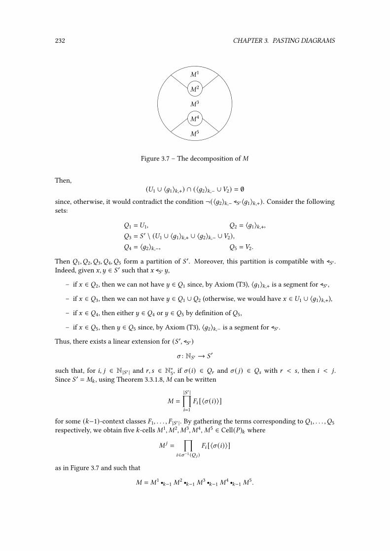
232 CHAPTER 3. PASTING DIAGRAMS

"1

"2

"3

"4

"5

Figure 3.7 – The decomposition of "

Then,(*1 ∪ 〈61〉:,+) ∩ (〈62〉:,− ∪+2) = ∅

since, otherwise, it would contradict the condition ¬(〈62〉:,− ⊳(′ 〈61〉:,+). Consider the followingsets:

&1 = *1, &2 = 〈61〉:,+,&3 = (

′ \ (*1 ∪ 〈61〉:,+ ∪ 〈62〉:,− ∪+2),&4 = 〈62〉:,−, &5 = +2.

Then &1, &2, &3, &4, &5 form a partition of ( ′. Moreover, this partition is compatible with ⊳(′ .Indeed, given G,~ ∈ ( ′ such that G ⊳(′ ~,

– if G ∈ &2, then we can not have ~ ∈ &1 since, by Axiom (T3), 〈61〉:,+ is a segment for ⊳(′ ,

– if G ∈ &3, then we can not have ~ ∈ &1 ∪&2 (otherwise, we would have G ∈ *1 ∪ 〈61〉:,+),

– if G ∈ &4, then either ~ ∈ &4 or ~ ∈ &5 by de�nition of &5,

– if G ∈ &5, then ~ ∈ &5 since, by Axiom (T3), 〈62〉:,− is a segment for ⊳(′ .

Thus, there exists a linear extension for (( ′, ⊳(′)

f : N(′ → ( ′

such that, for 8, 9 ∈ N |(′ | and A, B ∈ N∗5, if f (8) ∈ &A and f ( 9) ∈ &B with A < B , then 8 < 9 .Since ( ′ = ": , using Theorem 3.3.1.8, " can be written

" =

|(′ |∏8=1

�8 [〈f (8)〉]

for some (:−1)-context classes �1, . . . , � |(′ | . By gathering the terms corresponding to &1, . . . , &5respectively, we obtain �ve :-cells "1, "2, "3, "4, "5 ∈ Cell(%): where

" 9 =∏

8∈f−1 (& 9 )�8 [〈f (8)〉]

as in Figure 3.7 and such that

" = "1 r:−1 "

2 r:−1 "

3 r:−1 "

4 r:−1 "

5.

3.3. THE FREENESS PROPERTY 233

Sincem−:−1(!

1) = m−:−1(") = m

−:−1("

1) and !1:= *1 = "

1:,

by Lemma 3.3.1.4, we have !1 = "1. Moreover, since

m−:−1(�

′1 [〈61〉]) = m+:−1(!

1) = m+:−1("

1) = m−:−1("

2) and (� ′1 [m+: (〈61〉)]): = 〈61〉:,+ = "2:,

by Lemma 3.3.1.4, it implies that� ′1 [m+: (〈61〉)] = "2

Similarly, we can show that

� ′2 [m−: (〈62〉)] = "4 and '2 = "5.

Moreover, sincem−:−1(!

2) = m−:−1(") = m

−:−1("

1 r:−1 "

2 r:−1 "

3),

and

!2:= (2 \+2

= ( ′ \ (〈62〉:,− ∪+2)= &1 ∪&2 ∪&3,

by Lemma 3.3.1.4, we have!2 = "1 r

:−1 "2 r:−1 "

3.

Similarly, we have'1 = "3 r

:−1 "4 r:−1 "

5.

Hence, writting

�1 = È(!1, � ′1, id:� ′1 [m+:−1 ( 〈61 〉) ])É and �2 = È("3, � ′2, '

2)É

we have�1 = �1 r

:−1 �2 [m−: (62)] and �2 = �1 [m+: (61)] r:−1 �2

as wanted. �

From these two lemmas, we deduce that applied context classes are completely determined bytheir sources (or targets):

Theorem 3.3.2.3. Given :, = ∈ N with : < =, 6 ∈ %= and :-context classes �1, �2 of type 〈6〉 suchthat

m−:(�1 [〈6〉]) = m−: (�2 [〈6〉]) or m+

:(�1 [〈6〉]) = m+: (�2 [〈6〉]),

we have �1 = �2.

Proof. By symmetry, it is enough to prove the case where m−:(�1 [〈6〉]) = m−: (�2 [〈6〉]). We prove

this property by an induction on : . If : = 0, the result is trivial. So suppose that : > 0. Let

�1 = (!1, � ′1, '1) and �2 = (!2, � ′2, '

2)

be :-contexts such that �8 = È�8É for 8 ∈ {1, 2}. Thus,

!1 r:−1 �

′[m−:(〈6〉)] r:−1 '

1 = !2 r:−1 �

′[m−:(〈6〉)] r:−1 '

2

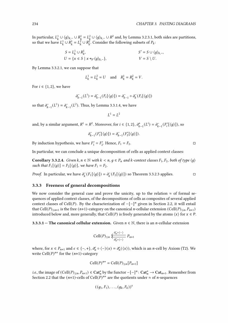
234 CHAPTER 3. PASTING DIAGRAMS

In particular, !1:∪ 〈6〉:,− ∪ '1

:= !2

:∪ 〈6〉:,− ∪ '2 and, by Lemma 3.2.3.1, both sides are partitions,

so that we have !1:∪ '1

:= !2

:∪ '2

:. Consider the following subsets of %: :

( = !1:∪ '1

:, ( ′ = ( ∪ 〈6〉:,−,

* = {G ∈ ( | G ⊳(′ 〈6〉:,−}, + = ( \* .

By Lemma 3.3.2.1, we can suppose that

!1:= !2

:= * and '1

:= '2

:= + .

For 8 ∈ {1, 2}, we have

m−:−1(!

8) = m−:−1(�8 [〈6〉]) = m

−:−1 ◦ m

−:(�8 [〈6〉])

so that m−:−1(!

1) = m−:−1(!

2). Thus, by Lemma 3.3.1.4, we have

!1 = !2

and, by a similar argument, '1 = '2. Moreover, for 8 ∈ {1, 2}, m+:−1(!

8) = m−:−1(�

′8 [〈6〉]), so

m−:−1(�

′1 [〈6〉]) = m−:−1(�

′2 [〈6〉]).

By induction hypothesis, we have � ′1 = �′2. Hence, �1 = �2. �

In particular, we can conclude a unique decomposition of cells as applied context classes:

Corollary 3.3.2.4. Given :, = ∈ N with : < =, 6 ∈ %= and :-context classes �1, �2, both of type 〈6〉such that �1 [〈6〉] = �2 [〈6〉], we have �1 = �2.

Proof. In particular, we have m−:(�1 [〈6〉]) = m−: (�2 [〈6〉]) so Theorem 3.3.2.3 applies. �

3.3.3 Freeness of general decompositions

We now consider the general case and prove the unicity, up to the relation ≈ of formal se-quences of applied context classes, of the decompositions of cells as composites of several appliedcontext classes of Cell(%). By the characterization of −[−]= given in Section 2.2, it will entailthat Cell(%)≤=+1 is the free (=+1)-category on the canonical =-cellular extension (Cell(%)≤=, %=+1)introduced below and, more generally, that Cell(%) is freely generated by the atoms 〈G〉 for G ∈ P.

3.3.3.1 — The canonical cellular extension. Given = ∈ N, there is an =-cellular extension

Cell(%)≤= %=+1m−=◦〈−〉

m+=◦〈−〉

where, for G ∈ %=+1 and n ∈ {−, +}, mn= ◦ 〈−〉(G) = mn= (〈G〉), which is an =-cell by Axiom (T2). Wewrite Cell(%)=+ for the (=+1)-category

Cell(%)=+ = Cell(%)≤= [%=+1]

i.e., the image of (Cell(%)≤=, %=+1) ∈ Cat+= by the functor −[−]= : Cat+= → Cat=+1. Remember fromSection 2.2 that the (=+1)-cells of Cell(%)=+ are the quotients under ≈ of =-sequences

((61, �1), . . . , (6: , �: ))s

3.3. THE FREENESS PROPERTY 235

where 68 ∈ %=+1 and �8 is an =-context class of type m−= (〈6〉) for 8 ∈ N∗:. For conciseness,

given 6 ∈ %=+1 and an =-context class of type m−= (〈6〉), we write � [6] for

� [6] = È((6, � ))sÉ ∈ (Cell(%)=+)=+1.

There is a morphism of =-cellular extension

(Cell(%)≤=, %=+1)(idCell(% )≤= , 〈−〉)−−−−−−−−−−−−→ (Cell(%)≤=,Cell(%)=+1)

which maps G ∈ %=+1 to 〈−〉(G) = 〈G〉. By the universal property of Cell(%)=+ discussed inSection 1.3.2, it induces a unique (=+1)-functor

eval= : Cell(%)=+ → Cell(%)≤=+1

often written eval for conciseness, such that

eval=≤= = idCell(% )≤= and eval(� [6]) = � [〈6〉]

for all 6 ∈ %=+1 and =-context class � of type m−= (〈6〉).

3.3.3.2 — Freeness of Cell(V). We now show the freeness of Cell(%) by proving the unicity ofdecomposition of cells as sequences of applied context classes up to the relation ≈. First, we showan analogous of Theorem 3.3.1.8, i.e., that the decompositions in Cell(%)=+ can also be reorderedby linear extensions:

Lemma 3.3.3.3. Let = ∈ N and - be an (=+1)-cell of Cell(%)=+ such that

- = �1 [G1] r= · · · r= �? [G?]for some ? ∈ N, G1, . . . , G? ∈ %=+1 and =-context classes �1, . . . , �? of Cell(%). Then, we havethat the function @ ↦→ G@ of type N∗@ → -=+1 is a linear extension of (-=+1, ⊳-=+1). Moreover,if f is a linear extension of (-=+1, ⊳-=+1), then there exist =-context classes �1, . . . , �? of respectivetypes 〈f (1)〉, . . . , 〈f (?)〉 such that

- = �1 [f (1)] r= · · · r= �? [f (?)] .Proof. Write d : N? → -=+1 for the function such that

d (8) = G8

for 8 ∈ N∗? . By the functoriality of eval, we have

eval(- ) = �1 [〈G1〉] r= · · · r= �? [〈G?〉]so that d is a linear extension by Proposition 3.3.1.10. We are left to prove the second part of thestatement. We have a morphism of linear extensions

5 = f−1 ◦ d

between f and d . By Lemma 3.3.1.2, we can suppose that 5 = g8,8+1 for some 8 ∈ N∗?−1. Toconclude, we only need to show that G8 and G8+1 can be swapped in the decomposition of -as �1 [G1] r= · · · r= �? [G?]. By contradiction, suppose that 〈G8〉=,+ ∩ 〈G8+1〉=,− ≠ ∅. In particular,we have d (8) ⊳-=+1 d (8 + 1). Since d = f ◦ g8,8+1, it implies f (8 + 1) ⊳-=+1 f (8). Thus, since f is a

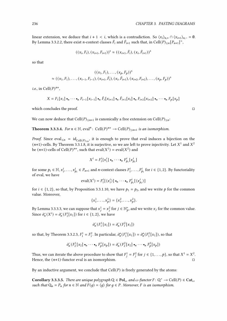
236 CHAPTER 3. PASTING DIAGRAMS

linear extension, we deduce that 8 + 1 < 8 , which is a contradiction. So 〈G8〉=,+ ∩ 〈G8+1〉=,− = ∅.By Lemma 3.3.2.2, there exist =-context classes �8 and �8+1 such that, in Cell(%)≤= [%=+1]≈,

((G8 , �8), (G8+1, �8+1))s ≈ ((G8+1, �8), (G8 , �8+1))s

so that

((G1, �1), . . . , (G? , �?))s

≈ ((G1, �1), . . . , (G8−1, �8−1), (G8+1, �8), (G8 , �8+1), (G8+2, �8+2), . . . , (G? , �?))s

i.e., in Cell(%)=+,

- = �1 [G1] r= · · · r= �8−1 [G8−1] r= �8 [G8+1] r= �8+1 [G8] r= �8+2 [G8+2] r= · · · r= �? [G?]which concludes the proof. �

We can now deduce that Cell(%)≤=+1 is canonically a free extension on Cell(%)≤= :

Theorem 3.3.3.4. For = ∈ N, eval= : Cell(%)=+ → Cell(%)≤=+1 is an isomorphism.

Proof. Since eval≤= = idCell(% )≤= , it is enough to prove that eval induces a bijection on the(=+1)-cells. By Theorem 3.3.1.8, it is surjective, so we are left to prove injectivity. Let - 1 and - 2

be (=+1)-cells of Cell(%)=+, such that eval(- 1) = eval(- 2) and

- 8 = � 81 [G81] r= · · · r= � 8?8 [G8?8 ]for some ?8 ∈ N, G81, . . . , G

8?8∈ %=+1 and =-context classes � 81, . . . , �

8?8

for 8 ∈ {1, 2}. By functorialityof eval, we have

eval(- 8) = � 81 [〈G81〉] r= · · · r= � 8?8 [〈G8?8 〉]for 8 ∈ {1, 2}, so that, by Proposition 3.3.1.10, we have ?1 = ?2, and we write ? for the commonvalue. Moreover,

{G11, . . . , G

1? } = {G2

1, . . . , G2? }.

By Lemma 3.3.3.3, we can suppose that G19 = G

29 for 9 ∈ N∗? , and we write G 9 for the common value.

Since m−= (- 8) = m−= (� 81 [G1]) for 8 ∈ {1, 2}, we have

m−= (� 11 [G1]) = m−= (� 2

1 [G1])

so that, by Theorem 3.3.2.3, � 11 = � 2

1 . In particular, m+= (� 11 [G1]) = m+= (� 2

1 [G1]), so that

m−= (� 12 [G2] r= · · · r= � 1

? [G?]) = m−= (� 22 [G2] r= · · · r= � 2

? [G?])

Thus, we can iterate the above procedure to show that � 19 = �

29 for 9 ∈ {1, . . . , ?}, so that - 1 = - 2.

Hence, the (=+1)-functor eval is an isomorphism. �

By an inductive argument, we conclude that Cell(%) is freely generated by the atoms:

Corollary 3.3.3.5. There are unique polygraphQ ∈ Poll andl-functor � : Q∗ → Cell(%) ∈ Catlsuch that Q= = %= for = ∈ N and � (6) = 〈6〉 for 6 ∈ % . Moreover, � is an isomorphism.

3.4. RELATING FORMALISMS 237

Proof. We show by induction on = ∈ N that there are unique =-polygraph Q= and morphism

�= : (Q=)∗ → Cell(%)≤=

such that Q=:= %: for : ∈ N and �= (6) = 〈6〉 for 6 ∈ Q= , and that �= is moreover an isomorphism.

This is clear for = = 0. So suppose that = > 0. If Q= and �= as above exist, then, by theunicity property of the induction hypothesis, we have Q=

≤=−1 = Q=−1 and �=≤=−1 = �=−1. The=-functor �= is then uniquely de�ned by the universal property of (Q=)∗ = (Q=−1)∗ [Q=] givenby Theorem 1.3.2.3 knowing that �= (6) = 〈6〉 for 6 ∈ Q=

= . Moreover, the =-polygraph structureon Q= is unique since

dn=−1(6) = (�=−1)−1 ◦ mn=−1(〈6〉) (3.27)

for6 ∈ Q== and n ∈ {−, +}. Finally, �= is an isomorphism since, by Theorem 3.3.3.4, (eval=−1)−1◦�=

is the image by −[−]=−1 of the isomorphism

(�=−1, 1%= ) : ((Q=−1)∗,Q== ) → (Cell(%)≤=−1, %=) ∈ Cat+=−1

so that the unicity of Q= and �= , and the fact that �= is an isomorphism are proved. For existence,one de�nes the =-polygraph structure on Q= from the one on Q=−1 and with (3.27), and the=-functor �= is then de�ned by extending �=−1, using the universal property of (Q=)∗.

Thus, by the de�nition of Poll and Proposition 1.2.3.12, we obtain unique l-polygraph Qand l-functor � : Q∗ → Cell(%), such that Q= = %= for = ∈ N and � (6) = 〈6〉, and � is moreoveran isomorphism. �

3.4 Relating formalisms

This section aims at relating all the introduced formalisms together. In particular, we show thatthe formalism of torsion-free complexes is a Rosetta stone that can express the other ones (aftercorrecting the defect of parity complexes and pasting schemes). Embedding parity complexesinto torsion-free complexes is almost direct, since they share the same de�nition of cells andseveral axioms. However, additional developments are needed for translating pasting schemesand augmented directed complexes into torsion-free complexes. Indeed, in the �rst case, oneneeds to show that a de�nition of cells analogous to the ones of pasting schemes can be usedfor torsion-free complexes before being able to relate the axioms of the two formalisms. In thesecond case, one needs to link the abelian group setting of augmented directed complexes to theset setting of torsion-free complexes.

We �rst introduce two other set-based de�nitions of cells for torsion-free complexes: closed-well-formed fgs’s and maximal-well-formed fgs’s (Section 3.4.1). The former is similar to thewell-formed fgs of pasting schemes, while the latter is a convenient intermediate between thecells of torsion-free complexes and closed-well-formed fgs’s. The l-categories of cells inducedby these two other de�nitions is then isomorphic to the one obtained with the initial de�nition(Theorems 3.4.1.24 and 3.4.1.27). Using the more natural de�nition of cells as closed-well-formedfgs’s, we give a characterization of polygraphs that can be represented by torsion-free complex(Theorem 3.4.1.29) and illustrate the use of torsion-free complexes with an extension of cateqthat enables to specify cells more easily (Paragraph 3.4.1.32). Next, we show the embeddings ofparity complexes (Section 3.4.2) and pasting schemes (Section 3.4.3) into torsion-free complexes.Then, we develop the relation between the set-based and group-based de�nitions of cells beforeshowing the embedding augmented directed complexes into torsion-free complexes (Section 3.4.4).Finally, we illustrate that those are the only embeddings between the formalisms by providingcounter-examples to the other ones (Section 3.4.5).

238 CHAPTER 3. PASTING DIAGRAMS

3.4.1 Closed and maximal cells

In this section, we introduce two other set-based de�nitions of cells for torsion-free complexes,namely closed-well-formed fgs’s and maximal-well-formed fgs’s, together with identity and com-positions operations for them. We moreover provide translation functions between the di�erentde�nitions of cells, and show that thel-categories of cells with the new de�nitions are isomorphicto the one with the original de�nition of cells (Theorems 3.4.1.24 and 3.4.1.27). Using this di�erentrepresentation, we characterize the polygraphs that can be represented by torsion-free complexes(Theorem 3.4.1.29). Finally, we illustrate the use of torsion-free complexes by introducing anextension of cateq based on closed-well-formed fgs’s (Paragraph 3.4.1.32).

3.4.1.1 — De�nitions. Let P be an l-hypergraph. Recall the de�nitions of fgs and closed fgsfrom Paragraph 3.1.3.6. We write

Closed(%)for the graded set of closed fgs’s of % . Given an =-fgs - of % , G ∈ - is said to be maximal in- when for all ~ ∈ % such that G R~ and G ≠ ~, it holds that ~ ∉ - . We write max(- ) for the=-fgs of % made of the maximal elements of - . The =-fgs - is then said to be maximal whenmax(- ) = - . We write

Max(%)for the gradet set of maximal fgs. Given = ∈ N and - an =-pre-cell of % , we write ∪- for the =-fgsof % given by

∪- =⋃8∈N=(-8,− ∪ -8,+).

3.4.1.2 — Maximality lemma. Let P be an l-hypergraph. In order to relate the cells of Cell(%)with the fgs’s of Max(%), we give here a simple criterion to characterize the maximal elements ina cell of Cell(%):

Lemma 3.4.1.3 (Maximality lemma). Suppose that % satis�es Axioms (T0), (T1), (T2) and (T3).Let :, = ∈ N with : < = and - ∈ Cell(%)= . For G ∈ -:,− (resp. G ∈ -:,+) with G not maximal in ∪- ,we have G ∈ -∓

:+1,− (resp. G ∈ -±:+1,+).

Proof. We prove this property by induction on ; = = − : . By symmetry, we only prove the casewhere G ∈ -:,−. Since G is not maximal, by de�nition of R, there exist

? ∈ N∗, [ ∈ {−, +}, G0, G1, . . . , G? ∈ % and n1, . . . , n? ∈ {−, +}

such thatG0 = G, G? ∈ -:+?,[ and G8 ∈ Gn8+18+1 for 8 ∈ N?−1.

Suppose that ? = 1. By Lemma 3.2.1.1, we have

-:,− ∩ - +:+1,[ = ∅.

Since G ∈ Gn11 and G1 ∈ -:+1,[ , we have

n1 = − and G ∈ -∓:+1,[ .

so that, by Lemma 3.2.1.5, G ∈ -∓:+1,−.

Otherwise, suppose that ? > 1. Let~ ∈ -:+?,[ be the smallest of-:+?,[ for ⊳-:+?,[ such that~ RG?−1.If G?−1 ∈ ~−, then, by minimality of ~, there is no ~ ∈ -:+?,[ such that G?−1 ∈ ~+. Therefore,

G?−1 ∈ -∓:+?,[ ⊆ -:+?−1,−.

3.4. RELATING FORMALISMS 239

Hence, G is not minimal in m−:+?−1(- ) and we conclude by induction. We now consider the

case G?−1 ∈ ~+. Let

� = {I ∈ -:+?,[ | I ⊳-:+?,[ ~} ∪ {~} and . = Act(m−:+?−1(- ),�).

We have G ∈ .:,− and G?−1 ∈ .:+?−1. Moreover, by Theorem 3.2.2.3, . is a cell. By inductionhypothesis, we have G ∈ .∓

:+1,−. Since -:+1,− and .:+1,− both move -:,− to -:,+, by Lemma 3.2.1.5,we have G ∈ -∓

:+1,− which concludes the proof. �

The above criterion gives a simple description of the set of maximal elements of a cell of Cell(%).

Lemma 3.4.1.4. Suppose that % satis�es Axioms (T0), (T1), (T2) and (T3). Let :, = ∈ N with : < =,an =-cell - ∈ Cell(%)= and n ∈ {−, +}. Then,

max(∪- ) ∩ %: = -:,− ∩ -:,+.

Proof. By Lemma 3.4.1.3,

max(∪- ) ∩ %: = (-:,− \ -∓:+1,−) ∪ (-:,+ \ -±:+1,+) .

By Lemma 3.2.1.6, it can be simpli�ed to

max(∪- ) ∩ %: = -:,− ∩ -:,+. �

3.4.1.5 — The translation functions. We now provide translation functions between the gradedsets Cell(%), Max(%) and Closed(%) and introduce several properties on them. The functions weintroduce are the ones represented on the diagram

Max(%)

PCell(%) Closed(%)

TMPC

TMCl

TPCCl

TPCM

TClM

TClPC

and are de�ned as follows:

– TPCM : PCell(%) → Max(%) is de�ned by

TPCM (- ) = max(∪- ) for - an =-pre-cell of % ,

– TMPC : Max(%) → PCell(%) is such that, for - an =-fgs of % , TM

PC(- ) is the =-pre-cell . of %de�ned by

.= = -=

and.8,− = -8 ∪ .∓8+1,− .8,+ = -8 ∪ .±8+1,+

for 8 ∈ N=−1,

– TMCl : Max(%) → Closed(%) is de�ned by

TMCl(- ) = R(- ) for - a maximal =-fgs of % ,

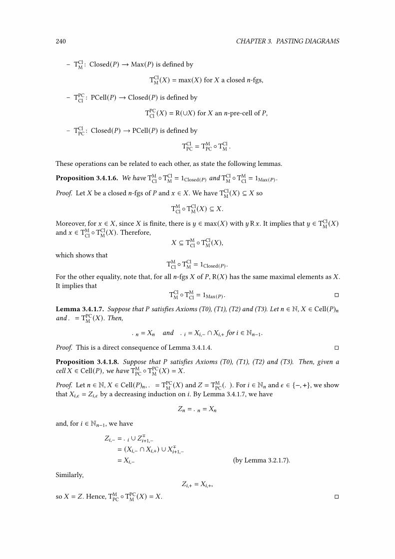
240 CHAPTER 3. PASTING DIAGRAMS

– TClM : Closed(%) → Max(%) is de�ned by

TClM (- ) = max(- ) for - a closed =-fgs,

– TPCCl : PCell(%) → Closed(%) is de�ned by

TPCCl (- ) = R(∪- ) for - an =-pre-cell of % ,

– TClPC : Closed(%) → PCell(%) is de�ned by

TClPC = TM

PC ◦TClM .

These operations can be related to each other, as state the following lemmas.

Proposition 3.4.1.6. We have TMCl ◦TCl

M = 1Closed(% ) and TClM ◦TM

Cl = 1Max(% ) .

Proof. Let - be a closed =-fgs of % and G ∈ - . We have TClM (- ) ⊆ - so

TMCl ◦TCl

M (- ) ⊆ - .

Moreover, for G ∈ - , since - is �nite, there is ~ ∈ max(- ) with ~ RG . It implies that ~ ∈ TClM (- )

and G ∈ TMCl ◦TCl

M (- ). Therefore,- ⊆ TM

Cl ◦TClM (- ),

which shows thatTM

Cl ◦TClM = 1Closed(% ) .

For the other equality, note that, for all =-fgs - of % , R(- ) has the same maximal elements as - .It implies that

TClM ◦TM

Cl = 1Max(% ) . �

Lemma 3.4.1.7. Suppose that % satis�es Axioms (T0), (T1), (T2) and (T3). Let = ∈ N, - ∈ Cell(%)=and . = TPC

M (- ). Then,

.= = -= and .8 = -8,− ∩ -8,+ for 8 ∈ N=−1.

Proof. This is a direct consequence of Lemma 3.4.1.4. �

Proposition 3.4.1.8. Suppose that % satis�es Axioms (T0), (T1), (T2) and (T3). Then, given acell - ∈ Cell(%), we have TM

PC ◦TPCM (- ) = - .

Proof. Let = ∈ N, - ∈ Cell(%)= , . = TPCM (- ) and / = TM

PC(. ). For 8 ∈ N= and n ∈ {−, +}, we showthat -8,n = /8,n by a decreasing induction on 8 . By Lemma 3.4.1.7, we have

/= = .= = -=

and, for 8 ∈ N=−1, we have

/8,− = .8 ∪ /∓8+1,−= (-8,− ∩ -8,+) ∪ -∓8+1,−= -8,− (by Lemma 3.2.1.7).

Similarly,/8,+ = -8,+,

so - = / . Hence, TMPC ◦TPC

M (- ) = - . �

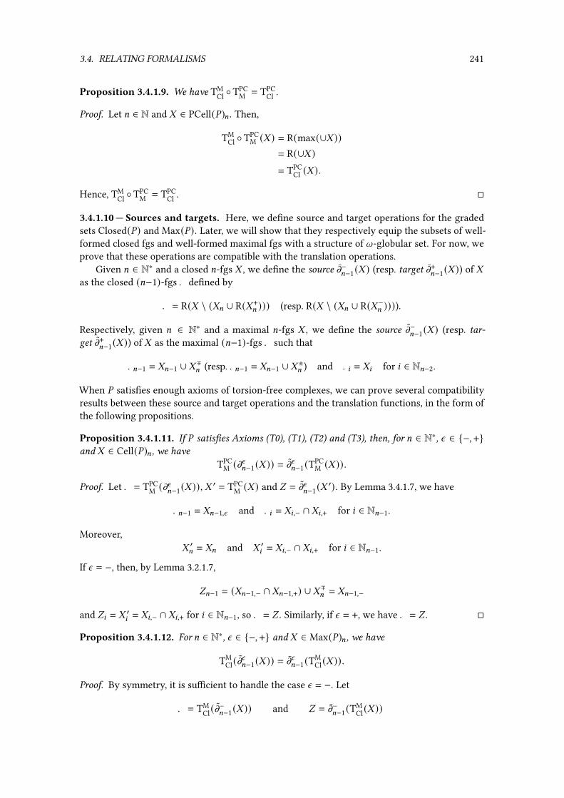
3.4. RELATING FORMALISMS 241

Proposition 3.4.1.9. We have TMCl ◦TPC

M = TPCCl .

Proof. Let = ∈ N and - ∈ PCell(%)= . Then,

TMCl ◦TPC

M (- ) = R(max(∪- ))= R(∪- )= TPC

Cl (- ) .

Hence, TMCl ◦TPC

M = TPCCl . �

3.4.1.10 — Sources and targets. Here, we de�ne source and target operations for the gradedsets Closed(%) and Max(%). Later, we will show that they respectively equip the subsets of well-formed closed fgs and well-formed maximal fgs with a structure of l-globular set. For now, weprove that these operations are compatible with the translation operations.

Given = ∈ N∗ and a closed =-fgs - , we de�ne the source m−=−1(- ) (resp. target m+=−1(- )) of -as the closed (=−1)-fgs . de�ned by

. = R(- \ (-= ∪ R(- += ))) (resp. R(- \ (-= ∪ R(-−= )))).

Respectively, given = ∈ N∗ and a maximal =-fgs - , we de�ne the source m−=−1(- ) (resp. tar-get m+=−1(- )) of - as the maximal (=−1)-fgs . such that

.=−1 = -=−1 ∪ -∓= (resp. .=−1 = -=−1 ∪ -±= ) and .8 = -8 for 8 ∈ N=−2.

When % satis�es enough axioms of torsion-free complexes, we can prove several compatibilityresults between these source and target operations and the translation functions, in the form ofthe following propositions.

Proposition 3.4.1.11. If % satis�es Axioms (T0), (T1), (T2) and (T3), then, for = ∈ N∗, n ∈ {−, +}and - ∈ Cell(%)= , we have

TPCM (m

n=−1(- )) = mn=−1(TPC

M (- )) .

Proof. Let . = TPCM (m

n=−1(- )), - ′ = TPC

M (- ) and / = mn=−1(- ′). By Lemma 3.4.1.7, we have

.=−1 = -=−1,n and .8 = -8,− ∩ -8,+ for 8 ∈ N=−1.

Moreover,- ′= = -= and - ′8 = -8,− ∩ -8,+ for 8 ∈ N=−1.

If n = −, then, by Lemma 3.2.1.7,

/=−1 = (-=−1,− ∩ -=−1,+) ∪ -∓= = -=−1,−

and /8 = - ′8 = -8,− ∩ -8,+ for 8 ∈ N=−1, so . = / . Similarly, if n = +, we have . = / . �

Proposition 3.4.1.12. For = ∈ N∗, n ∈ {−, +} and - ∈ Max(%)= , we have

TMCl(m

n=−1(- )) = mn=−1(TM

Cl(- )) .

Proof. By symmetry, it is su�cient to handle the case n = −. Let

. = TMCl(m

−=−1(- )) and / = m−=−1(TM

Cl(- )).

242 CHAPTER 3. PASTING DIAGRAMS

By unfolding the de�nitions, we have

. = R((- \ -=) ∪ -∓= ) and / = R(R(- ) \ (-= ∪ R(- += ))).

In order to show that . ⊆ / , we only need to prove that . ′ ⊆ / where

. ′ = (- \ -=) ∪ -∓= .

First, we have that . ′ ⊆ R(- ). Moreover,

. ′ ∩ (-= ∪ R(- += ))= ((- \ -=) ∪ -∓= ) ∩ (-= ∪ R(- += ))= ((- \ -=) ∪ -∓= ) ∩ R(- += )= (- \ -=) ∩ R(- += )= - ∩ R(- += )= ∅ (since - is maximal).

So . ′ ⊆ / , which implies that . ⊆ / .

Similarly, in order to show that / ⊆ . , we only need to prove that / ′ ⊆ . where

/ ′ = R(- ) \ (-= ∪ R(- += )).

But/ ′ ⊆ . ⇔ R(- ) ⊆ . ∪ -= ∪ R(- += )

and

. ∪ -= ∪ R(- += ) = R((- \ -=) ∪ -∓= ) ∪ -= ∪ R(- += )= R((- \ -=) ∪ -∓= ∪ - += ) ∪ -== R((- \ -=) ∪ -−= ∪ - += ) ∪ -== R((- \ -=) ∪ -−= ∪ - += ∪ -=)= R(- ) .

So / ′ ⊆ . , which implies that / ⊆ . . Hence, . = / , which concludes the proof. �

Proposition 3.4.1.13. If % satis�es Axioms (T0), (T1), (T2) and (T3), then, for = ∈ N∗, n ∈ {−, +}and - ∈ Cell(%)= ,

TPCCl (m

n=−1(- )) = mn=−1(TPC

Cl (- )) .

Proof. We have

TPCCl (m

n=−1(- )) = TM

Cl ◦TPCM (m

n=−1(- )) (by Proposition 3.4.1.9)

= TMCl(m

n=−1(TPC

M (- ))) (by Proposition 3.4.1.11)= mn=−1(TM

Cl ◦TPCM (- )) (by Proposition 3.4.1.12)

= mn=−1(TPCCl (- ))

which concludes the proof. �

3.4. RELATING FORMALISMS 243

3.4.1.14 — Identities and compositions. Here, we de�ne identity and composition operationsfor the graded sets Max(%) and Closed(%), and prove some compatibility results with the transla-tions functions.

Given = ∈ N and a closed (resp. maximal) =-fgs - , we de�ne the identity of - as the closed(resp. maximal) (=+1)-fgs id=+1(- ) de�ned by

id=+1(- ) = (-0, . . . , -=, ∅) .

Given 8, = ∈ N with 8 < = and two maximal =-fgs -,. , we de�ne the maximal 8-composition of -and . as the maximal =-fgs - ∗M8 . de�ned by

- ∗M8 . = max(R(- ) ∪ R(. )).

Respectively, given 8, = ∈ Nwith 8 < = and two closed=-fgs-,. , we de�ne the closed 8-compositionof - and . as the closed =-fgs - ∗Cl

8 . de�ned by

- ∗Cl8 . = - ∪ . .

For simplicity, we sometimes write ∗Cl (resp. ∗M) for ∗Cl8 (resp. ∗M8 ). We now prove several com-

patibility results of the identity and composition operations with the translation functions.

Proposition 3.4.1.15. For = ∈ N and an =-cell - ∈ Cell(%),

TPCCl (id

=+1(- )) = id=+1(TPCCl (- )) .

Proof. It readily follows from the de�nitions. �

Proposition 3.4.1.16. For = ∈ N and an =-cell - ∈ Cell(%),

TPCM (id

=+1(- )) = id=+1(TPCM (- )) .

Proof. It readily follows from the de�nitions. �

Proposition 3.4.1.17. For 8, = ∈ N with 8 < =, and 8-composable =-cells - and . in Cell(%),

TPCCl (- ∗8 . ) = TPC

Cl (- ) ∗Cl8 TPC

Cl (. ) .

Proof. Let / = - ∗8 . . We haveTPC

Cl (- ∗8 . ) = R(∪/ )

andTPC

Cl (- ) ∗Cl8 TPC

Cl (. ) = R(∪- ) ∪ R(∪. ) = R((∪- ) ∪ (∪. )) .

By de�nition of composition, ∪/ ⊆ (∪- ) ∪ (∪. ), so

TPCCl (- ∗8 . ) ⊆ TPC

Cl (- ) ∗Cl8 TPC

Cl (. ) .

For the other inclusion, note that - 9,n ⊆ / 9,n for 9 ∈ N= and n ∈ {−, +} with ( 9, n) ≠ (8, +), and

-8,+ = (-8,− ∪ - +8+1,−) \ -−8+1,−⊆ /8,− ∪ /+8+1,−⊆ R(∪/ )

244 CHAPTER 3. PASTING DIAGRAMS

so ∪- ⊆ R(∪/ ). Similarly, ∪. ⊆ R(∪/ ), thus

(∪- ) ∪ (∪. ) ⊆ R(∪/ ),

which implies thatTPC

Cl (- ) ∗Cl8 TPC

Cl (. ) ⊆ TPCCl (- ∗8 . ) .

Hence,TPC

Cl (- ) ∗Cl8 TPC

Cl (. ) = TPCCl (- ∗8 . ) . �

Proposition 3.4.1.18. For 8, = ∈ N with 8 < =, and -,. ∈ Closed(%)= ,

TClM (- ∗

Cl8 . ) = TCl

M (- ) ∗M8 TCl

M (. ) .

Proof. We have

TClM (- ) ∗

M8 TCl

M (. ) = max(R(TClM (- )) ∪ R(TCl

M (. )))= max(- ∪ . ) (by Proposition 3.4.1.6)

= TClM (- ∗

Cl8 . )

which concludes the proof. �

Proposition 3.4.1.19. For 8, = ∈ N with 8 < =, and 8-composable =-cells - and . of % ,

TPCM (- ∗8 . ) = TPC

M (- ) ∗M8 TPC

M (. ) .

Proof. We have

TPCM (- ∗8 . ) = TCl

M ◦TPCCl (- ∗8 . ) (by Propositions 3.4.1.6 and 3.4.1.9)

= TClM (T

PCCl (- ) ∗

Cl8 TPC

Cl (. )) (by Proposition 3.4.1.13)

= TClM ◦TPC

Cl (- ) ∗M8 TCl

M ◦TPCCl (. ) (by Proposition 3.4.1.18)

= TPCM (- ) ∗

M8 TPC

M (. ) (by Propositions 3.4.1.6 and 3.4.1.9)

which concludes the proof. �

3.4.1.20 —Well-formed cells. We de�ned above source, target, identity and composition oper-ations for both Closed(%) and Max(%). However, these operations are not expected to equip thegraded sets Closed(%) and Max(%) with a structure of l-category (in fact, not even a structure ofl-globular set). In order to obtain an l-category, we need to restrict to subsets of “well-formed”elements of Closed(%) and Max(%). Then, we can show that the two induced l-category of cellsare isomorphic to Cell(%).

Let % be an l-hypergraph. Given = ∈ N and - ∈ Closed(%)= , we say that - is closed-well-formedwhen

– -= is fork-free,

– m−=−1(- ) and m+=−1(- ) are closed-well-formed,

– if = ≥ 2, m−=−2 ◦ m−=−1(- ) = m−=−2 ◦ m+=−1(- ) and m+=−2 ◦ m−=−1(- ) = m+=−2 ◦ m+=−1(- ).

We write ClosedWF(%) for the graded set of closed-well-formed fgs of % . Respectively, given = ∈ Nand - ∈ Max(%)= , we say that - is maximal-well-formed when

3.4. RELATING FORMALISMS 245

– -= is fork-free,

– m−=−1(- ) and m+=−1(- ) are maximal-well-formed,

– if = ≥ 2, m−=−2 ◦ m−=−1(- ) = m−=−2 ◦ m+=−1(- ) and m+=−2 ◦ m−=−1(- ) = m+=−2 ◦ m+=−1(- ).

We write MaxWF(%) for the graded set of maximal-well-formed fgs of % . We now aim at provingthat both ClosedWF(%) and MaxWF(%) are l-categories isomorphic to Cell(%) when % satis�esenough axioms of torsion-free complexes. We �rst show this property for MaxWF(%) after intro-ducing several technical results.

Lemma 3.4.1.21. If % satis�es Axioms (T0), (T1), (T2) and (T3), then, for = ∈ N and - ∈ Cell(%)= ,we have TPC

M (- ) ∈ MaxWF(%)= .

Proof. We proceed by induction on =. If = = 0, the result is trivial. So suppose that = > 0 andlet . = TPC

M (- ). Since .= = -= , .= is fork-free. Moreover, by Proposition 3.4.1.11, we have

mn=−1(. ) = TPCM (m

n=−1(- )) for n ∈ {−, +}.

By the induction hypothesis, mn=−1(. ) is maximal-well-formed. And, when = ≥ 2, for [ ∈ {−, +},we have

m[

=−2 ◦ m−=−1(. ) = TPC

M (m[

=−2 ◦ m−=−1(- )) (by Proposition 3.4.1.11)

= TPCM (m

[

=−2 ◦ m+=−1(- ))

= m[

=−2 ◦ m+=−1(. ) .

Hence, . is maximal-well-formed. �

Lemma 3.4.1.22. If % satis�es Axioms (T0), (T1), (T2) and (T3), then, for= ∈ N and- ∈ MaxWF(%)= ,there exists an =-cell . ∈ Cell(%)= such that TPC

M (. ) = - .

Proof. We proceed by induction on =. If = = 0, the result is trivial. So suppose that = > 0. Byinduction, let (,) ∈ Cell(%)=−1 be such that TPC

M (() = m−=−1(- ) and TPCM () ) = m+=−1(- ). When

= ≥ 2, for n ∈ {−, +}, we have

mn=−2(() = TMPC ◦TPC

M (mn=−2(()) (by Proposition 3.4.1.8)

= TMPC(m

n=−2(TPC

M (())) (by Proposition 3.4.1.11)= TM

PC(mn=−2 ◦ m−=−1(- ))

= TMPC(m

n=−2 ◦ m+=−1(- )) (because - is maximal-well-formed)

= TMPC(m

n=−2(TPC

M () )))= TM

PC ◦TPCM (m

n=−2() ))

= mn=−2() ) .

Moreover,

((=−1 ∪ - += ) \ -−= = (-=−1 ∪ -∓= ∪ - += ) \ -−== -=−1 ∪ -±== )=−1.

Similarly, ()=−1 ∪ -−= ) \ - += = (=−1 so -= moves (=−1 to )=−1. Hence, the =-pre-cell . de�ned by

.= = -=, .=−1,− = (=−1, .=−1,+ = )=−1 and .8,X = (8,X for 8 ∈ N=−2 and X ∈ {−, +}

246 CHAPTER 3. PASTING DIAGRAMS

is an =-cell. Let / = TPCM (. ). We have /= = -= and

m−=−1(/ ) = m−=−1(TPCM (. ))

= TPCM (m

−=−1(. )) (by Proposition 3.4.1.11)

= TPCM (()

= m−=−1(- ).

So, by de�nition of m−, we have

/=−1 ∪ -∓= = -=−1 ∪ -∓= and /8 = -8 for 8 ∈ N=−2.

Since - and / are maximal, we have

-=−1 ∩ -∓= = /=−1 ∩ -∓= = ∅.

Hence, -=−1 = /=−1 and - = / = TPCM (. ) which concludes the proof. �

Lemma 3.4.1.23. If % satis�es Axioms (T0), (T1), (T2) and (T3), then, TPCM induces a bijection

between Cell(%) and MaxWF(%).

Proof. By Lemma 3.4.1.22, TPCM : Cell(%) → MaxWF(%) is surjective and, by Proposition 3.4.1.8, it

is injective, so it is bijective. �

We can now deduce that maximal-well-formed fgs’s are an adequate alternative de�nition of cellsfor torsion-free complexes:

Theorem 3.4.1.24. If % satis�es Axioms (T0), (T1), (T2) and (T3), then, MaxWF(%) is an l-categoryand TPC

M induces an isomorphism between Cell(%) and MaxWF(%).

Proof. By de�nition of MaxWF(%), the functions m−:, m+:

for : ∈ N equip MaxWF(%) with a struc-ture of l-globular set. We �rst prove that the composition operation ∗M restricts to MaxWF(%).Let 8, = ∈ N with 8 < =, and -,. ∈ MaxWF(%)= be such that m+8 (- ) = m−8 (. ). By Lemma 3.4.1.23,there exist - ′, . ′ ∈ Cell(%)= such that TPC

M (-′) = - and TPC

M (.′) = . . By Proposition 3.4.1.11, we

haveTPC

M (m+8 (- ′)) = m+8 (- ) = m−8 (. ) = TPC

M (m−8 (. ′)),

and, by Lemma 3.4.1.23, m+8 (- ′) = m−8 (. ′) so - ′ and . ′ are 8-composable. By Lemma 3.4.1.23, wehave TPC

M (-′ ∗8 . ′) ∈ MaxWF(%) and, by Proposition 3.4.1.19, - ∗M8 . ∈ MaxWF(%).

By Propositions 3.4.1.11, 3.4.1.16 and 3.4.1.19, TPCM commutes with the source, target, identity

and composition operations and is a bijection when restricted to MaxWF(%), so that MaxWF(%)is an l-category since Cell(%) is (by Theorem 3.2.3.3 and Remark 3.2.3.4), and TPC

M induces anisomorphism of l-categories. �

We prove a similar property for closed-well-formed fgs’s after showing some technical results.

Lemma 3.4.1.25. TMCl induces a bijection between MaxWF(%) and ClosedWF(%).

Proof. We already know that TMCl is a bijection by Proposition 3.4.1.6. For = ∈ N, we show that TM

Clsends a maximal-well-formed =-fgs - to a closed-well-formed =-fgs by induction on =. If = = 0,the result is trivial. So suppose that = > 0. Let . = TM

Cl(- ). Then, .= = -= is fork-free and,

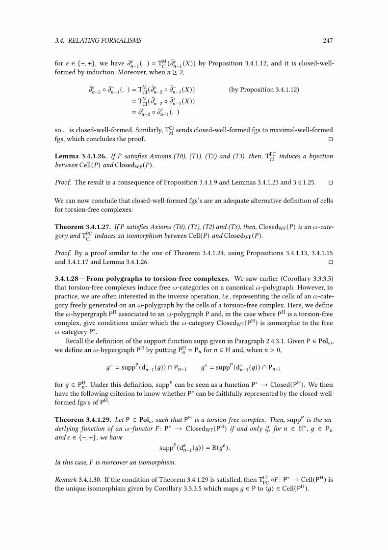
3.4. RELATING FORMALISMS 247

for n ∈ {−, +}, we have mn=−1(. ) = TMCl(m

n=−1(- )) by Proposition 3.4.1.12, and it is closed-well-

formed by induction. Moreover, when = ≥ 2,

mn=−2 ◦ m−=−1(. ) = TMCl(m

n=−2 ◦ m−=−1(- )) (by Proposition 3.4.1.12)

= TMCl(m

n=−2 ◦ m+=−1(- ))

= mn=−2 ◦ m+=−1(. )

so . is closed-well-formed. Similarly, TClM sends closed-well-formed fgs to maximal-well-formed

fgs, which concludes the proof. �

Lemma 3.4.1.26. If % satis�es Axioms (T0), (T1), (T2) and (T3), then, TPCCl induces a bijection

between Cell(%) and ClosedWF(%).

Proof. The result is a consequence of Proposition 3.4.1.9 and Lemmas 3.4.1.23 and 3.4.1.25. �

We can now conclude that closed-well-formed fgs’s are an adequate alternative de�nition of cellsfor torsion-free complexes:

Theorem 3.4.1.27. If % satis�es Axioms (T0), (T1), (T2) and (T3), then, ClosedWF(%) is an l-cate-gory and TPC

Cl induces an isomorphism between Cell(%) and ClosedWF(%).

Proof. By a proof similar to the one of Theorem 3.4.1.24, using Propositions 3.4.1.13, 3.4.1.15and 3.4.1.17 and Lemma 3.4.1.26. �

3.4.1.28 — From polygraphs to torsion-free complexes. We saw earlier (Corollary 3.3.3.5)that torsion-free complexes induce free l-categories on a canonical l-polygraph. However, inpractice, we are often interested in the inverse operation, i.e., representing the cells of an l-cate-gory freely generated on an l-polygraph by the cells of a torsion-free complex. Here, we de�nethe l-hypergraph PH associated to an l-polygraph P and, in the case where PH is a torsion-freecomplex, give conditions under which the l-category ClosedWF(PH) is isomorphic to the freel-category P∗.

Recall the de�nition of the support function supp given in Paragraph 2.4.3.1. Given P ∈ Poll ,we de�ne an l-hypergraph PH by putting PH

= = P= for = ∈ N and, when = > 0,

6− = suppP(d−=−1(6)) ∩ P=−1 6+ = suppP(d+=−1(6)) ∩ P=−1

for 6 ∈ PH= . Under this de�nition, suppP can be seen as a function P∗ → Closed(PH). We then

have the following criterion to know whether P∗ can be faithfully represented by the closed-well-formed fgs’s of PH:

Theorem 3.4.1.29. Let P ∈ Poll such that PH is a torsion-free complex. Then, suppP is the un-derlying function of an l-functor � : P∗ → ClosedWF(PH) if and only if, for = ∈ N∗, 6 ∈ P=and n ∈ {−, +}, we have

suppP(dn=−1(6)) = R(6n ).

In this case, � is moreover an isomorphism.

Remark 3.4.1.30. If the condition of Theorem 3.4.1.29 is satis�ed, then TClPC ◦� : P∗ → Cell(PH) is

the unique isomorphism given by Corollary 3.3.3.5 which maps 6 ∈ P to 〈6〉 ∈ Cell(PH).

248 CHAPTER 3. PASTING DIAGRAMS

Proof. If suppP induces an l-functor � : P∗ → ClosedWF(PH), then we have

suppP(dn=−1(6)) = � (dn=−1(6))= mn=−1(� (6))= mn=−1(R(6))= R(6n ) (by de�nition of mn=−1)

which proves the necessity. For su�ciency, we prove by induction on = ∈ N that suppP is theunderlying function of an =-functor �= : (P∗)≤= → ClosedWF(PH)≤= . This is clear for = = 0, and,when= > 0, we de�ne �= by extending �=−1 and so that �= (6) = R(6) using the universal propertyof (P∗)≤= = (P∗)≤=−1 [P=]. This is possible since the condition of the statement implies that

�=−1(dn=−1(6)) = mn=−1(R(6))

for 6 ∈ P= and n ∈ {−, +}. We then obtain an l-functor � : P∗ → ClosedWF(PH) using Proposi-tion 1.2.3.12, which satis�es that � (6) = R(6) for 6 ∈ P. Then, by Theorem 3.4.1.27, TCl

PC ◦� is anl-functor P∗ → Cell(%) which maps 6 to 〈6〉. It is then an isomorphism by Corollary 3.3.3.5, sothat � is an isomorphism too. �

Example 3.4.1.31. Let P be the l-polygraph with

P0 = {G,~, I} P1 = {5 : G → ~ 6,6′ : ~ → I} P2 = {U, U ′ : 6⇒ 6′}P3 = {� : id2

5∗0 U ⇒ id2

5U ′}

and P: = ∅ for : ∈ N with : ≥ 4 as in

G ~ I5

6

6′

U ⇓ ⇓U ′ and G I

5 ∗06

5 ∗06′

⇓ id25∗0U

�≡V G I

5 ∗06

5 ∗06′

⇓ id25∗0U ′ .

We can verify that PH is a torsion-free complex. But, by Theorem 3.4.1.29, the function suppPdoes not induce an l-functor P∗ → ClosedWF(PH) since

suppP(d−2 (�)) = {G,~, I, 5 , 6, 6′, U} ≠ {~, I, 6, 6′, U} = R(�−).

However, by considering a modi�ed version of P where

P3 = {� : U ⇒ U ′}

it can be veri�ed that PH is still a torsion-free complex and that, by Theorem 3.4.1.29, the func-tion suppP induces an l-functor P∗ → ClosedWF(PH) which is an isomorphism.

3.4.1.32 — A pasting diagram extension for cateq. We illustrate the use of pasting diagramsby describing an extension of cateq that allows specifying cells using pasting diagrams or, moreprecisely, closed-well-formed fgs’s of torsion-free complexes.

For example, consider the l-hypergraph (3.1) on page 189. It can be veri�ed that it is atorsion-free complex. The associated l-polygraph is then described in cateq by the followingcommands:

3.4. RELATING FORMALISMS 249

# u,v,w,x,y := gen *# a := gen u -> v# b,c,d := gen v -> w# e,f,g := gen w -> x# h := gen x -> y# alpha := gen b -> c# beta := gen c -> d# gamma := gen e -> f# delta := gen f -> g

Then, as suggested back there, the cell composing “all the generators together” can be de�nedwith the expressions

# X1 := id2 a *0 (alpha *1 beta)*0 ((gamma *0 id2 h) *1 (delta *0 id2 h))

and

# X2 := (id2 a *0 alpha *0 id2 e *0 id2 h)*1 (id2 a *0 id2 c *0 gamma *0 id2 h)*1 (id2 a *0 beta *0 delta *0 id2 h)

and one can verify that the answer of cateq on the query

# X1 = X2

is true . We can de�ne this cell using pasting diagrams with the syntax {[gen1],[gen2],...}as in

# X3 := {u,v,w,x,y,a,b,c,d,e,f,g,h,alpha,beta,gamma,delta}

and one veri�es that cateq answers true on the query X2 = X3 . In fact, cateq applies theclosure operator R on a pasting diagram input, so that it is su�cient to specify the maximumelements. Thus, we can de�ne

# X4 := {a,alpha,beta,gamma,delta,h}

and verify that X3 = X4 evaluates to true . We are allowed to mix the pasting diagram syntaxwith the usual syntax and write a query like

# id2 a *0 {alpha,beta,gamma,delta} *0 id2 h = X4

which cateq evaluates to true .

Let’s now look at another example and see how to specify the cells �1 and �2 associated withthe l-hypergraph % of Paragraph 3.1.2.13 using pasting diagram syntax. We can already use thissyntax to specify the generators, as in

# x,y,z := gen *# a,b,c := gen x -> y# d,e,f := gen y -> z# alpha,alpha' := gen a -> b

250 CHAPTER 3. PASTING DIAGRAMS

# beta,beta' := gen b -> c# gamma,gamma' := gen d -> e# delta,delta' := gen e -> f# A := gen {alpha,delta} -> {alpha',delta'}# B := gen {beta,gamma} -> {beta',gamma'}

Then, �1 and �2 can be de�ned with

# H1 := {beta,A,gamma} *2 {alpha',B,delta'}# H2 := {alpha,B,delta} *2 {gamma',A,beta'}

which is more economical than the expression used in Paragraph 3.1.2.13. Note that, even though %is not a torsion-free complex, the de�nition of H1 is accepted. Indeed, cateq allows the use ofthe pasting diagram syntax for a local expression when the sub-l-hypergraph induced by the ex-pression is a torsion-free complex. For example, the two sets of generators {V,�,W} and {U ′, �, X ′}induce two sub-l-hypergraphs (by applying the R operation) of P that are torsion-free complexes,so that the de�nition of H1 is accepted by cateq. However, cateq refuses the de�nition of Hdone by command

# H := {A,B}

since the sub-l-hypergraph induced by {�, �} (which is % ) is not a torsion-free complex.Remark 3.4.1.33. In fact, cateq checks that an l-hypergraph is a torsion-free complex using thestronger Axioms (T3’) and (T4’), since they are more e�ciently computed. As a consequence,it might miss some torsion-free complexes that only satisfy Axioms (T3) and (T4) but not thestronger ones.Remark 3.4.1.34. When provided with a command involving a pasting diagram syntax, cateqveri�es that the condition given by Theorem 3.4.1.29 is satis�ed with regard to the current poly-graph, and otherwise refuses the command and alerts the user, so that the use of pasting diagramsyntax in cateq is always safe.

3.4.2 Embedding parity complexes

In this section, we show that parity complexes are a particular case of torsion-free complexes,under two reasonable caveats. Firstly, since parity complexes do not require all the generatorsto be relevant, there are parity complexes that are not torsion-free complexes. But, by [Str91,Theorem 4.2], irrelevant generators of a parity complex % do not play any role in the generatedl-category Cell(%), so that, by restraining % to the l-hypergraph % of relevant generators, wehave Cell(%) = Cell(%). Thus, it is reasonable to assume that all the parity complexes we are con-sidering for embedding in torsion-free complexes have relevant generators, i.e., satisfy Axiom (T2).Secondly, as discussed in Paragraph 3.1.5.4, general parity complexes are not freely generated bytheir atoms and, since the latter property is supposed to be the raison d’être of such structures,it is reasonable to only consider the parity complexes that satisfy this property. We believe thatAxiom (T4) is the minimal additional condition to require for the l-category of cells of a paritycomplex to be freely generated, so we will only consider parity complexes that moreover satisfyAxiom (T4).

Under the assumptions given above, we are only left to derive Axiom (T3) from the axioms of aparity complex. We show below that it is essentially a consequence of the tightness requirementsstated by Axiom (C5). First, we recall from [Str94] the link between tightness and the segmentproperty:

3.4. RELATING FORMALISMS 251

Proposition 3.4.2.1 ([Str94, Proposition 1.4]). Let % be an l-hypergraph. For = ∈ N∗, subsets* ,+ ⊆ %= with* tight, + fork-free and* ⊆ + , we have that* is a segment for ⊳+ .

Proof. Let G,~, I ∈ + such that G, I ∈ * and G ⊳1+~ ⊳+ I. Then, there isF ∈ G+ ∩ ~−. By de�nition

of tightness, since ~ ⊳+ I, we have ~− ∩* ± = ∅. So there is ~ ∈ * such that F ∈ ~−. Since + isfork-free, ~ = ~. Hence,* is a segment for ⊳+ . �

Then, we show how to derive the segment property from the axioms of parity complexes:

Lemma 3.4.2.2. Let % be a parity complex which satis�es Axiom (T2). Given = ∈ N and G ∈ %= , Gsatis�es the segment condition.

Proof. Let :, = ∈ N with : < =, G ∈ %= and - be a :-cell. Suppose �rst that 〈G〉:,− ⊆ -: . ByAxiom (C5), the set 〈G〉:,− is tight, so that, by Proposition 3.4.2.1, 〈G〉:,− is a segment for ⊳-: .

Now suppose that 〈G〉:,+ ⊆ -: . By contradiction, assume that 〈G〉:,+ is not a segment for ⊳-: .By de�nition of ⊳-: , there exist ? > 1 and D0, . . . , D? ∈ -: such that

D0, D? ∈ 〈G〉:,+, D1, . . . , D?−1 ∉ 〈G〉:,+ and D8 ⊳1-:D8+1.

By de�nition of ⊳1-:

, there exist I0, . . . , I?−1 such that I8 ∈ D+8 ∩D−8+1. Note that I0 ∈ 〈G〉±:,+. Indeed,if I0 ∈ E− for some E ∈ -: , then, since -: is fork-free, E = D1, so E ∉ 〈G〉:,+. Similarly, wehave I?−1 ∈ 〈G〉∓:,+. Since G is relevant by Axiom (T2), we have

〈G〉±:+1,+ = 〈G〉:,+ ⊆ -:

By [Str91, Lemma 3.2] (which is the analogous for parity complexes of Theorem 3.2.2.3) andAxiom (T2), we have that

〈G〉:,− ∩ -= ⊆ 〈G〉−:+1,+ ∩ -= = ∅

and the :-pre-cell . = Act(-, 〈G〉:+1,+) is a :-cell. Moreover, by Lemma 3.2.1.6,

.: = (-: ∪ 〈G〉−:+1,+) \ 〈G〉+:+1,+ = (-: \ 〈G〉:,+) ∪ 〈G〉:,−.

Thus, 〈G〉:,− ⊆ .: and, as shown by the �rst part, 〈G〉:,− is a segment for ⊳.: . Since

〈G〉∓:,− = 〈G〉

∓:,+ and 〈G〉±

:,− = 〈G〉±:,+,

there exist D0, D? ∈ 〈G〉:,− such that I0 ∈ D+0 and I?−1 ∈ D−? . So

D0 ⊳1-:D1 ⊳

1-:· · · ⊳1

-:D?−1 ⊳

1-:D?

with D1, . . . , D?−1 ∉ 〈G〉:,− (since 〈G〉−:+1,+ ∩-= = ∅), contradicting the fact that 〈G〉:,− is a segment

for ⊳.: . Thus, 〈G〉:,+ is a segment for ⊳-: . Hence, G satis�es the segment condition. �

We can conclude that parity complexes are embedded into torsion-free complexes:

Theorem 3.4.2.3. Given a parity complex % which satis�es Axiom (T2) and Axiom (T4), % is atorsion-free complex.

Proof. Axiom (T0) is a consequence of Axiom (C0). Axiom (T1) is a consequence of Axiom (C3).And Axiom (T3) is a consequence of Lemma 3.4.2.2. �

Remark 3.4.2.4. Given % as in Theorem 3.4.2.3, the category Cell(%) of cells of the parity complex %is, of course, exactly the category Cell(%) of cells of the torsion-free complex % .

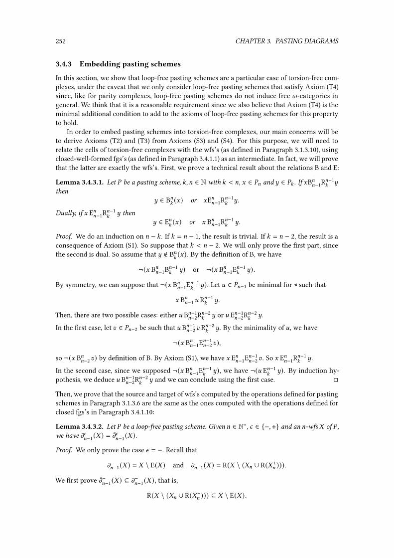
252 CHAPTER 3. PASTING DIAGRAMS

3.4.3 Embedding pasting schemes

In this section, we show that loop-free pasting schemes are a particular case of torsion-free com-plexes, under the caveat that we only consider loop-free pasting schemes that satisfy Axiom (T4)since, like for parity complexes, loop-free pasting schemes do not induce free l-categories ingeneral. We think that it is a reasonable requirement since we also believe that Axiom (T4) is theminimal additional condition to add to the axioms of loop-free pasting schemes for this propertyto hold.

In order to embed pasting schemes into torsion-free complexes, our main concerns will beto derive Axioms (T2) and (T3) from Axioms (S3) and (S4). For this purpose, we will need torelate the cells of torsion-free complexes with the wfs’s (as de�ned in Paragraph 3.1.3.10), usingclosed-well-formed fgs’s (as de�ned in Paragraph 3.4.1.1) as an intermediate. In fact, we will provethat the latter are exactly the wfs’s. First, we prove a technical result about the relations B and E:

Lemma 3.4.3.1. Let % be a pasting scheme, :, = ∈ N with : < =, G ∈ %= and ~ ∈ %: . If GB==−1R=−1:~

then~ ∈ B=

:(G) or GE==−1R=−1

:~.

Dually, if G E==−1R=−1:

~ then~ ∈ E=

:(G) or G B==−1R=−1

:~.

Proof. We do an induction on = − : . If : = = − 1, the result is trivial. If : = = − 2, the result is aconsequence of Axiom (S1). So suppose that : < = − 2. We will only prove the �rst part, sincethe second is dual. So assume that ~ ∉ B=

:(G). By the de�nition of B, we have

¬(G B==−1B=−1:

~) or ¬(G B==−1E=−1:

~).

By symmetry, we can suppose that ¬(G B==−1E=−1:

~). Let D ∈ %=−1 be minimal for ⊳ such that

G B==−1D R=−1:

~.

Then, there are two possible cases: either D B=−1=−2R=−2

:~ or D E=−1

=−2R=−2:

~.

In the �rst case, let E ∈ %=−2 be such that D B=−1=−2 E R=−2

:~. By the minimality of D, we have

¬(G B==−1E=−1=−2 E),

so ¬(G B==−2 E) by de�nition of B. By Axiom (S1), we have G E==−1E=−1=−2 E . So G E==−1R=−1

:~.

In the second case, since we supposed ¬(G B==−1E=−1:

~), we have ¬(D E=−1:

~). By induction hy-pothesis, we deduce D B=−1

=−2R=−2:

~ and we can conclude using the �rst case. �

Then, we prove that the source and target of wfs’s computed by the operations de�ned for pastingschemes in Paragraph 3.1.3.6 are the same as the ones computed with the operations de�ned forclosed fgs’s in Paragraph 3.4.1.10:

Lemma 3.4.3.2. Let % be a loop-free pasting scheme. Given = ∈ N∗, n ∈ {−, +} and an =-wfs - of % ,we have mn=−1(- ) = mn=−1(- ).

Proof. We only prove the case n = −. Recall that

m−=−1(- ) = - \ E(- ) and m−=−1(- ) = R(- \ (-= ∪ R(- += ))).

We �rst prove m−=−1(- ) ⊆ m−=−1(- ), that is,

R(- \ (-= ∪ R(- += ))) ⊆ - \ E(- ) .

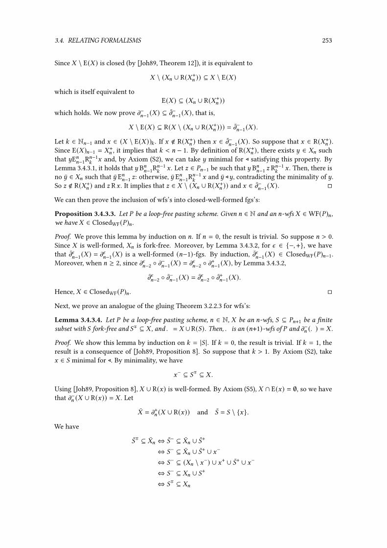
3.4. RELATING FORMALISMS 253

Since - \ E(- ) is closed (by [Joh89, Theorem 12]), it is equivalent to

- \ (-= ∪ R(- += )) ⊆ - \ E(- )

which is itself equivalent toE(- ) ⊆ (-= ∪ R(- += ))

which holds. We now prove m−=−1(- ) ⊆ m−=−1(- ), that is,

- \ E(- ) ⊆ R(- \ (-= ∪ R(- += ))) = m−=−1(- ).

Let : ∈ N=−1 and G ∈ (- \ E(- )): . If G ∉ R(- += ) then G ∈ m−=−1(- ). So suppose that G ∈ R(- += ).Since E(- )=−1 = - += , it implies that : < = − 1. By de�nition of R(- += ), there exists ~ ∈ -= suchthat ~E==−1R=−1

:G and, by Axiom (S2), we can take ~ minimal for ⊳ satisfying this property. By

Lemma 3.4.3.1, it holds that ~ B==−1R=−1:

G . Let I ∈ %=−1 be such that ~ B==−1 I R=−1:

G . Then, there isno ~ ∈ -= such that ~ E==−1 I: otherwise, ~ E==−1R=−1

:G and ~ ⊳~, contradicting the minimality of ~.

So I ∉ R(- += ) and I RG . It implies that I ∈ - \ (-= ∪ R(- += )) and G ∈ m−=−1(- ). �

We can then prove the inclusion of wfs’s into closed-well-formed fgs’s:

Proposition 3.4.3.3. Let % be a loop-free pasting scheme. Given = ∈ N and an =-wfs - ∈ WF(%)= ,we have - ∈ ClosedWF(%)= .

Proof. We prove this lemma by induction on =. If = = 0, the result is trivial. So suppose = > 0.Since - is well-formed, -= is fork-free. Moreover, by Lemma 3.4.3.2, for n ∈ {−, +}, we havethat mn=−1(- ) = mn=−1(- ) is a well-formed (=−1)-fgs. By induction, mn=−1(- ) ∈ ClosedWF(%)=−1.Moreover, when = ≥ 2, since mn=−2 ◦ m−=−1(- ) = mn=−2 ◦ m+=−1(- ), by Lemma 3.4.3.2,

mn=−2 ◦ m−=−1(- ) = mn=−2 ◦ m+=−1(- ).

Hence, - ∈ ClosedWF(%)= . �

Next, we prove an analogue of the gluing Theorem 3.2.2.3 for wfs’s:

Lemma 3.4.3.4. Let % be a loop-free pasting scheme, = ∈ N, - be an =-wfs, ( ⊆ %=+1 be a �nitesubset with ( fork-free and (∓ ⊆ - , and . = - ∪R((). Then, . is an (=+1)-wfs of % and m−= (. ) = - .

Proof. We show this lemma by induction on : = |( |. If : = 0, the result is trivial. If : = 1, theresult is a consequence of [Joh89, Proposition 8]. So suppose that : > 1. By Axiom (S2), takeG ∈ ( minimal for ⊳. By minimality, we have

G− ⊆ (∓ ⊆ - .

Using [Joh89, Proposition 8], - ∪ R(G) is well-formed. By Axiom (S5), - ∩ E(G) = ∅, so we havethat m−= (- ∪ R(G)) = - . Let

- = m+= (- ∪ R(G)) and ( = ( \ {G}.

We have

(∓ ⊆ -= ⇔ (− ⊆ -= ∪ (+

⇔ (− ⊆ -= ∪ (+ ∪ G−

⇔ (− ⊆ (-= \ G−) ∪ G+ ∪ (+ ∪ G−

⇔ (− ⊆ -= ∪ (+

⇔ (∓ ⊆ -=

254 CHAPTER 3. PASTING DIAGRAMS

so (∓ ⊆ - . By induction, - ∪ R(() is well-formed and m−= (- ∪ R(()) = - . Since WF(%) has thestructure of an l-category by [Joh89, Theorem 12], we can compose - ∪ R(G) and - ∪ R((). So

- ∪ R(() = - ∪ R(G) ∪ - ∪ R(()

is well-formed and m−= (- ∪ R(()) = - . �

We can now prove the converse inclusion of closed-well-formed fgs’s into wfs’s:

Proposition 3.4.3.5. Let % be a loop-free pasting scheme. Given = ∈ N and - ∈ ClosedWF(%)= , wehave - ∈ WF(%)= .

Proof. We prove this lemma by induction on =. If = = 0, the result is trivial. So suppose = > 0.Let . = m−=−1(- ). By de�nition of ClosedWF(%), . ∈ ClosedWF(%) and, by induction, . ∈ WF(%).By de�nition of m−, we have -∓= ⊆ . . Moreover, by Lemma 3.4.3.4, . ∪ R(-=) is well-formed.But . = R(- \ (-= ∪ R(- += ))), so that - = . ∪ R(-=) is well-formed. �

We now give a simple form for the sources and targets of atomic wfs’s:

Lemma 3.4.3.6. Let % be a loop-free pasting scheme. Given 8, = ∈ N such that 8 < =, n ∈ {−, +}and G ∈ %= , we have

mn8 (R(G)) = R(〈G〉8,n ) .

Proof. By symmetry, we can suppose that n = −. We have

m−8 (R(G)) = m−8 (TMCl({G}))

= TMCl(m

−8 ({G})) (by Proposition 3.4.1.12 and Lemma 3.4.3.2)

= TMCl(〈G〉8,−)

= R(〈G〉8,−) .

Hence, m−8 (R(G)) = R(〈G〉8,−). �

Using the above lemma, we deduce the relevance of the generators:

Lemma 3.4.3.7. Let % be a loop-free pasting scheme. Given = ∈ N and G ∈ %= , G is relevant.

Proof. By Axiom (S3), R(G) is well-formed. So, for 8 ∈ N=−1 and n ∈ {−, +}, mn8 (R(G)) is well-formed. Then, by Lemma 3.4.3.6, 〈G〉8,− and 〈G〉8,+ are fork-free. We show that 〈G〉±8+1,− = 〈G〉8,+and 〈G〉∓8+1,+ = 〈G〉8,−. We have

〈G〉±=,− = 〈G〉± = G+ = 〈G〉=−1,+

and, similarly, 〈G〉∓=,+ = 〈G〉=−1,−. For 8 ∈ N=−1, we have

〈G〉±8+1,− = (m+8 (R(〈G〉8+1,−)))8 (by de�nition of m+8 )= (m+8 ◦ m−8+1(R(G)))8 (by Lemma 3.4.3.6)= (m+8 (R(G)))8 (by globularity)= (R(〈G〉8,+))8 (by Lemma 3.4.3.6)= 〈G〉8,+

3.4. RELATING FORMALISMS 255

and similarly, 〈G〉∓8+1,+ = 〈G〉8,−. Moreover, we have

(〈G〉8,− ∪ 〈G〉+8+1,−) \ 〈G〉−8+1,− = ((〈G〉−8+1,− \ 〈G〉+8+1,−) ∪ 〈G〉+8+1,−) \ 〈G〉−8+1,−= 〈G〉+8+1,− \ 〈G〉−8+1,− = 〈G〉8,+

and(〈G〉8,+ ∪ 〈G〉−8+1,−) \ 〈G〉+8+1,− = ((〈G〉+8+1,− \ 〈G〉−8+1,−) ∪ 〈G〉−8+1,−) \ 〈G〉+8+1,−

= 〈G〉−8+1,− \ 〈G〉+8+1,− = 〈G〉8,−so 〈G〉8+1,− moves 〈G〉8,− to 〈G〉8,+ and, similarly, so does 〈G〉8+1,+. Hence, 〈G〉 is a cell. �

We now prove that the cells (in the sense of Paragraph 3.1.2.4) of pasting schemes are sent towfs’s by TPC

Cl , and that all the generators satisfy the segement condition:

Lemma 3.4.3.8. Let % be a loop-free pasting scheme and = ∈ N. The following hold:

(i) for G ∈ %= , G satis�es the segment condition,

(ii) for - ∈ Cell(%)= , TPCCl (- ) ∈ WF(%)= .

Proof. We prove this lemma by an induction on =. If = = 0, the result is trivial. So supposethat = > 0.

We �rst prove (i). Let : ∈ N=−1, G ∈ %= , - be a :-cell such that 〈G〉:,− ⊆ -: , and . = TPCCl (- ).

By induction, . ∈ WF(%). Moreover, by Lemma 3.4.3.6,

m−:(R(G)) = R(〈G〉:,−) ⊆ . .

So, by Axiom (S4), 〈G〉:,− is a segment for ⊳.: = ⊳-: . Hence, G satis�es the segment condition.We now prove (ii). Let - ∈ Cell(%)= . By Proposition 3.4.3.5, it is enough to show that TPC

Cl (- )is closed-well-formed. This latter property can be obtained from Theorem 3.4.1.27 which requiresthe full segment axiom. But we can consider the restriction of % to an l-hypergraph % where

%8 = %8 for 8 ≤ = and %8 = ∅ for 8 > =.

By (i), % satis�es Axiom (T3). Then, using Theorem 3.4.1.27, TPCCl (- ) is closed-well-formed and is

still closed-well-formed in % . Hence, by Proposition 3.4.3.5, TPCCl (- ) ∈ WF(%). �

We can conclude the embedding of pasting schemes into torsion-free complexes:

Theorem 3.4.3.9. Let % be a loop-free pasting scheme. Then, % satis�es Axioms (T0), (T1), (T2)and (T3). In particular, if % satis�es Axiom (T4), then % is a torsion-free complex.

Proof. The di�erent axioms of torsion-free complexes can be deduced as follows: Axiom (T0)is a consequence of Axiom (S0), Axiom (T1) is a consequence of Axiom (S2), Axiom (T2) is aconsequence of Lemma 3.4.3.7 and Axiom (T3) is a consequence of Lemma 3.4.3.8. �

Moreover, one translates the cells of the pasting scheme to the wfs’s using the operation TPCCl :

Theorem 3.4.3.10. Let % be a loop-free pasting scheme. TPCCl is an isomorphism between the l-cate-

gories Cell(%) and WF(%). Moreover, for all G ∈ % , TPCCl (〈G〉) = R(G).

Proof. By Propositions 3.4.3.3 and 3.4.3.5, we have

ClosedWF(%) = WF(%)as graded sets and, by Lemma 3.4.3.2 and the de�nition of id, ∗Cl and ∗, the two have the samestructure of l-category. Thus, by Theorems 3.4.3.9 and 3.4.1.27, TPC

Cl : Cell(%) → WF(%) is anisomorphism. Moreover, by Proposition 3.4.1.9, for G ∈ % , we have

TPCCl (〈G〉) = TM

Cl ◦TPCM (〈G〉) = TM

Cl({G}) = R(G). �

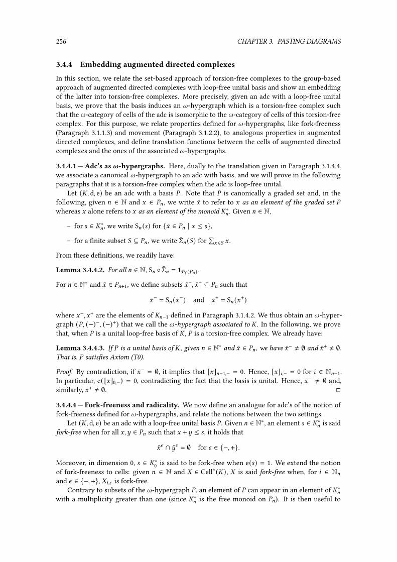
256 CHAPTER 3. PASTING DIAGRAMS

3.4.4 Embedding augmented directed complexes

In this section, we relate the set-based approach of torsion-free complexes to the group-basedapproach of augmented directed complexes with loop-free unital basis and show an embeddingof the latter into torsion-free complexes. More precisely, given an adc with a loop-free unitalbasis, we prove that the basis induces an l-hypergraph which is a torsion-free complex suchthat the l-category of cells of the adc is isomorphic to the l-category of cells of this torsion-freecomplex. For this purpose, we relate properties de�ned for l-hypergraphs, like fork-freeness(Paragraph 3.1.1.3) and movement (Paragraph 3.1.2.2), to analogous properties in augmenteddirected complexes, and de�ne translation functions between the cells of augmented directedcomplexes and the ones of the associated l-hypergraphs.

3.4.4.1 — Adc’s as 8-hypergraphs. Here, dually to the translation given in Paragraph 3.1.4.4,we associate a canonical l-hypergraph to an adc with basis, and we will prove in the followingparagraphs that it is a torsion-free complex when the adc is loop-free unital.

Let ( , d, e) be an adc with a basis % . Note that % is canonically a graded set and, in thefollowing, given = ∈ N and G ∈ %= , we write G to refer to G as an element of the graded set %whereas G alone refers to G as an element of the monoid ∗= . Given = ∈ N,

– for B ∈ ∗= , we write S= (B) for {G ∈ %= | G ≤ B},

– for a �nite subset ( ⊆ %= , we write Σ= (() for∑G ∈( G .

From these de�nitions, we readily have:

Lemma 3.4.4.2. For all = ∈ N, S= ◦ Σ= = 1Pf (%=) .

For = ∈ N∗ and G ∈ %=+1, we de�ne subsets G−, G+ ⊆ %= such that

G− = S= (G−) and G+ = S= (G+)

where G−, G+ are the elements of =−1 de�ned in Paragraph 3.1.4.2. We thus obtain an l-hyper-graph (%, (−)−, (−)+) that we call the l-hypergraph associated to . In the following, we provethat, when % is a unital loop-free basis of , % is a torsion-free complex. We already have:

Lemma 3.4.4.3. If % is a unital basis of , given = ∈ N∗ and G ∈ %= , we have G− ≠ ∅ and G+ ≠ ∅.That is, % satis�es Axiom (T0).

Proof. By contradiction, if G− = ∅, it implies that [G]=−1,− = 0. Hence, [G]8,− = 0 for 8 ∈ N=−1.In particular, e( [G]0,−) = 0, contradicting the fact that the basis is unital. Hence, G− ≠ ∅ and,similarly, G+ ≠ ∅. �

3.4.4.4 — Fork-freeness and radicality. We now de�ne an analogue for adc’s of the notion offork-freeness de�ned for l-hypergraphs, and relate the notions between the two settings.

Let ( , d, e) be an adc with a loop-free unital basis % . Given = ∈ N∗, an element B ∈ ∗= is saidfork-free when for all G,~ ∈ %= such that G + ~ ≤ B , it holds that

Gn ∩ ~n = ∅ for n ∈ {−, +}.

Moreover, in dimension 0, B ∈ ∗0 is said to be fork-free when e(B) = 1. We extend the notionof fork-freeness to cells: given = ∈ N and - ∈ Cell∗( ), - is said fork-free when, for 8 ∈ N=and n ∈ {−, +}, -8,n is fork-free.

Contrary to subsets of the l-hypergraph % , an element of % can appear in an element of ∗=with a multiplicity greater than one (since ∗= is the free monoid on %=). It is then useful to

3.4. RELATING FORMALISMS 257

distinguish the elements of ∗= where generators appear with multiplicity at most one: given= ∈ Nand B ∈ ∗= , B is said radical when for all I ∈ ∗= such that 2I ≤ B , we have I = 0. We then readilyhave:

Lemma 3.4.4.5. For all = ∈ N and B ∈ ∗= radical, Σ= ◦ S= (B) = B

Moreover, fork-freeness implies radicality:

Lemma 3.4.4.6. Given = ∈ N and B ∈ ∗= , if B is fork-free, then B is radical.

Proof. If = = 0, B ∈ ∗= can be written B =∑

1≤8≤: G8 for some : ∈ N and G8 ∈ %0 for 8 ∈ N∗:.

So e(B) = : , and, by fork-freeness, : = 1. Hence, B is radical.Otherwise, assume that = > 0. By contradiction, suppose that there is G ∈ %= such that 2G ≤ B .

By Lemma 3.4.4.3, it means that G− ∩ G− ≠ ∅, contradicting the fact that B is fork-free. Hence, B isradical. �

Like for cells of torsion-free complexes, cells of adc’s with loop-free basis are fork-free:

Lemma 3.4.4.7. Given = ∈ N and - ∈ Cell∗( )= , - is fork-free.

Proof. We prove this lemma using an induction on =. If = = 0, since e(-0) = 1, - is fork-free byde�nition.

Otherwise, suppose that = > 0. By induction, m−=−1(- ) and m+=−1(- ) are fork-free, so -8,n isfork-free for 8 ∈ N=−1 and n ∈ {−, +}. Let G, ~ ∈ %= be such that G + ~ ≤ -= . By contradiction,suppose that there is I ∈ %=−1 such that I ∈ G− ∩ ~−. By [Ste04, Proposition 5.4], there are

: ≥ 1, G1, . . . , G: ∈ %= and - 1, . . . , -: ∈ Cell∗( )

with - 8= = G8 for 8 ∈ N∗:

and such that

- = - 1 ∗=−1 · · · ∗=−1 -:

so -= = G1 + · · · + G: . Hence, there are 1 ≤ 81, 82 ≤ : with 81 ≠ 82 such that G81 = G and G82 = ~. Bysymmetry, we can suppose that 81 < 82. If there is some 8 such that I ∈ G+8 , by [Ste04, Proposition5.4], we have 8 < 81. So, for 81 ≤ 8 ≤ 82, it holds that I ∉ G+8 . Let . = - 81 ∗=−1-

81+1 ∗=−1 · · · ∗=−1-82 .

We have that . ∈ Cell∗( ) and

.=−1,− =∑

81≤8≤82[G8]=−1,− −

∑81≤8≤82

[G8]=−1,+ + .=−1,+

with2I ≤

∑81≤8≤82

[G8]=−1,− and ¬(I ≤∑

81≤8≤82[G8]=−1,+) and .=−1,+ ≥ 0

so 2I ≤ .=−1,−, contradicting the fact that m−=−1(. ) is radical by Lemma 3.4.4.6. Thus G− ∩ ~− = ∅and, similarly, G+ ∩ ~+ = ∅. Hence, - is fork-free. �

We now give several compatibility results for the operations Σ= with sets and the structure ofl-hypergraph on % :

Lemma 3.4.4.8. Let = ∈ N,* ,+ ⊆ %= be �nite subsets and G ∈ %= . The following hold:

(i) if* ∩+ = ∅, then Σ= (* ) ∧ Σ= (+ ) = 0 and Σ= (* ∪+ ) = Σ= (* ) + Σ= (+ ),

(ii) if* ⊆ + , then Σ= (* ) ≤ Σ= (+ ) and Σ= (+ \* ) = Σ= (+ ) − Σ= (* ),

258 CHAPTER 3. PASTING DIAGRAMS

(iii) if = > 0, then Σ=−1(Gn ) = Gn ,

(iv) Suppose that * is fork-free. Then Σ= (* ) is fork-free. Moreover, in the case where = > 0, wehave Σ=−1(* n ) = (Σ= (* ))n .

Proof. (i) and (ii) are direct consequences of the de�nitions. For (iii), note that Gn = S=−1(Gn ). ByLemma 3.4.4.7, [G]=−1,n is fork-free and, by Lemma 3.4.4.6, it is radical. So, by Lemma 3.4.4.5, wehave Σ=−1(Gn ) = Gn .

For (iv), suppose that* ⊆ %= is fork-free. If = = 0, the result is trivial. So suppose that = > 0.Given G,~ ∈ %= with G ≤ Σ= (* ) and ~ ≤ Σ= (* ), I ∈ %=−1 and n ∈ {−, +} such that I ≤ Gnand I ≤ ~n , we have I ∈ Gn and I ∈ ~n . Since * is fork-free, G = ~. Also, Σ= (* ) is radical byde�nition of Σ= , so that ¬(G + ~ ≤ Σ= (* )). Hence, Σ= (* ) is fork-free. For the second part, notethat, for G,~ ∈ * with G ≠ ~, we have Gn ∩ ~n = ∅. Hence,

Σ=−1(* n ) = Σ=−1(∪G ∈* Gn )=

∑G ∈*

Σ=−1(Gn ) (by (i))

=∑G ∈*

Gn (by (iii))

= (Σ= (* ))n . �

We give analogous compatibility results for the operations S= with the group structure of = andthe operations (−)− and (−)+ de�ned on = :

Lemma 3.4.4.9. Let = ∈ N, D, E ∈ ∗= be such that D, E are radical and I ∈ %= . The following hold:

(i) if D ∧ E = 0, then S= (D) ∩ S= (E) = ∅ and S= (D + E) = S= (D) ∪ S= (E),

(ii) if D ≤ E , then S= (D) ⊆ S= (E) and S= (E − D) = (S= (E)) \ (S= (D)),

(iii) if = > 0, then S=−1(In ) = In ,

(iv) Suppose that D is fork-free. Then, S= (D) is fork-free. Moreover, in the case where = > 0, wehave S=−1(Dn ) = (S= (D))n .

Proof. (i), (ii) and (iii) are direct consequences of the de�nitions. For (iv), suppose that D is fork-free. If= = 0, the result is trivial, so suppose that= > 0. Given G, ~ ∈ S= (D), I ∈ P=−1 and n ∈ {−, +}such that I ∈ Gn ∩ ~n , we have I ≤ Gn and I ≤ ~n . By fork-freeness, ¬(G + ~ ≤ D). But G ≤ Dand ~ ≤ D, so that G = ~. Thus, S= (D) is fork-free. For the second part, note that, for G,~ ∈ %=with G ≠ ~, G ≤ D and ~ ≤ D, we have Gn ∧ ~n = 0. Hence,

S=−1(Dn ) = S=−1(∑

G ∈%=,G≤DGn )

=⋃

G ∈%=,G≤DS=−1(Gn ) (by (i))

=⋃

G ∈%=,G≤DGn (by (iii))

= (S= (D))n . �

3.4. RELATING FORMALISMS 259

3.4.4.10 — Movement properties. We now relate the movement properties of l-hypergraphs(Paragraph 3.1.2.2) to properties of augmented directed complexes. Such results will be requiredfor proving the correspondence between the cells of l-hypergraphs and the cells of augmenteddirected complexes.

Let ( , d, e) be an adc with a loop-free unital basis % . We �rst prove a compatibility result ofthe functions Σ= with the operations (−)∓ and (−)± on l-hypergraphs and adc’s:

Lemma 3.4.4.11. Let = ∈ N∗, D ∈ ∗= fork-free and* = S= (D). We have

D∓ = Σ=−1(* ∓) and D± = Σ=−1(* ±) .

Proof. We have

d(D) = D± − D∓

= D+ − D−

= Σ=−1(* +) − Σ=−1(* −) (by Lemma 3.4.4.8)= (Σ=−1(* ±)+ Σ=−1(* + ∩* −))− (Σ=−1(* ∓) + Σ=−1(* + ∩* −)) (by Lemma 3.4.4.8)

= Σ=−1(* ±) − Σ=−1(* ∓) .

Since* ± ∩* ∓ = ∅, we have Σ=−1(* ±) ∧ Σ=−1(* ∓) = ∅. By uniqueness of the decomposition,

D∓ = Σ=−1(* ∓) and D± = Σ=−1(* ±) . �

Now, we show a compatibility of the operations Σ= with movement:

Lemma 3.4.4.12. Let = ∈ N, ( ⊆ %=+1 be a �nite and fork-free set and* ,+ ⊆ %= be �nite sets suchthat ( moves* to + . Then, d(Σ=+1(()) = Σ= (+ ) − Σ= (* ).

Proof. By de�nition of movement, + = (* ∪ (+) \ (−. Hence,

Σ= (+ ) = Σ= ((* ∪ (+) \ (−)= Σ= (* ∪ (+) − Σ= ((−) (by Lemma 3.4.4.8, since (− ⊆ * ∪ (+)= Σ= (* ) + Σ= ((+) − Σ= ((−) (since* ∩ (+ = ∅ by Lemma 3.2.1.1)= Σ= (* ) + (Σ=+1(())+ − (Σ=+1(())− (by Lemma 3.4.4.8)= Σ= (* ) + d(Σ=+1(()) . �

Conversely, we prove su�cient conditions for the operations S= to induce movement:

Lemma 3.4.4.13. Let = ∈ N, B ∈ ∗=+1 fork-free, D, E ∈ ∗= with D, E radical, such that

d(B) = E − D, D ∧ B+ = 0 and B− ∧ E = 0.

Then, S=+1(B) moves S= (D) to S= (E).

Proof. Let ( = S=+1(B),* = S= (D) and + = S= (E). Since d(B) = E − D, we have

B− ≤ B− + E = D + B+

so(− = S= (B−) ⊆ S= (D + B+) = * ∪ (+.

260 CHAPTER 3. PASTING DIAGRAMS

Thus,

Σ= ((* ∪ (+) \ (−) = Σ= (* ∪ (+) − Σ= ((−)= Σ= ◦ S= (D + B+) − B− (by Lemma 3.4.4.8)= D + B+ − B−

= D + d(B)= E

= Σ= (+ )

so, by Lemma 3.4.4.2,+ = (* ∪(+) \(− . Similarly,* = (+ ∪(−) \(+. Hence, ( moves* to+ . �

Finally, we show empty intersection results for cells of Cell∗( ), whose analogous for Cell(%)hold:

Lemma 3.4.4.14. Let = ∈ N∗ and - ∈ Cell∗( )= . Then, for 8 ∈ N=−1 and n ∈ {−, +}, we have

-8,− ∧ - +8+1,n = 0 and -−8+1,n ∧ -8,+ = 0.

Proof. By contradiction, suppose given = ∈ N∗, - ∈ Cell∗( )= , 8 ∈ N=−1 and n ∈ {−, +} that givea counter-example for this property. By applying m−, m+ su�ciently, we can suppose that 8 = =− 1.Also, by symmetry, we only need to handle the �rst case, that is, when there is I ∈ %=−1 suchthat I ≤ -=−1,− ∧ - += . So there is G ∈ %= such that G ≤ -= and I ≤ G+. By the de�nition of a cell,we have d(-=) = -=−1,+ − -=−1,−, thus

-=−1,+ +∑

D∈%=,D≤-=D− = -=−1,− +

∑D∈%=,D≤-=

D+

≥ 2I

and, since -=−1,+ is radical, there is ~ ∈ %= with ~ ≤ -= such that I ≤ ~−. By [Ste04, Proposi-tion 5.1], there are : ∈ N∗, G1, . . . , G: ∈ %= with G1 + · · · + G: = -= , 81, 82 ∈ N∗: with 81 < 82, G81 = Gand G82 = ~, and - 1, . . . , -: ∈ Cell∗( ) with - 8= = G8 for 8 ∈ N∗

:such that - = - 1 ∗=−1 · · · ∗=−1 -

: .Let . = - 1 ∗=−1 · · · ∗=−1 -

81 . Since . is a cell, we have

.=−1,+ +∑

1≤8≤:G−8 = .=−1,− +

∑1≤8≤:

G+8

= -=−1,− +∑

1≤8≤:G+8

≥ 2I.

Moreover, since - is fork-free and I ≤ G−82 , we have ¬(I ≤ G−8 ) for 8 ∈ N81 . So 2I ≤ .=−1,+,contradicting the fact that.=−1,+ is radical by Lemmas 3.4.4.7 and 3.4.4.6. Hence,-8,− ∧ - += = 0. �

3.4.4.15 — The translation operations. We now introduce translation functions between thecells of augmented directed complexes and the cells of their associated l-hypergraphs, and showthat these translations are bijective.

Let ( , d, e) be an adc with a loop-free unital basis % . We extend the operations Σ= and S=to translation functions between the pre-cells of % and the pre-cells of . Given = ∈ N andan =-pre-cell - ∈ PCell(%)= , we de�ne Σ(- ) ∈ Cell∗( ) as the =-pre-cell . such that

.8,n = Σ8 (-8,n ) for 8 ∈ N= and n ∈ {−, +}.

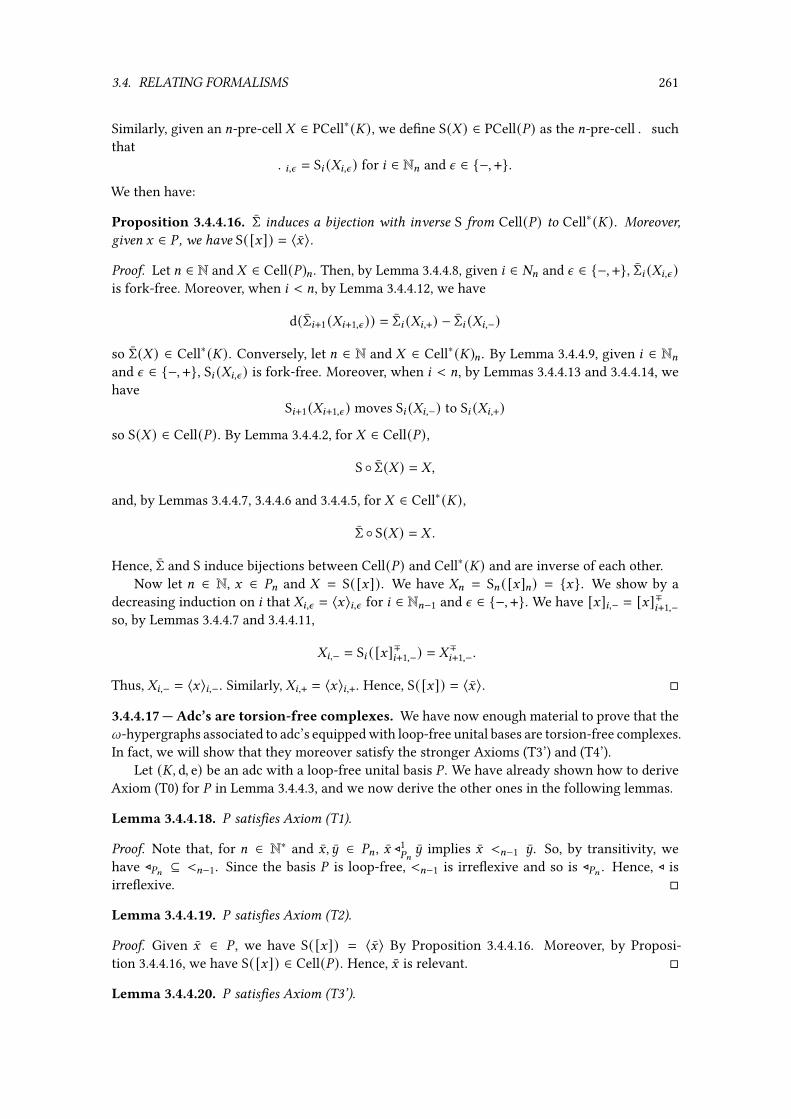
3.4. RELATING FORMALISMS 261

Similarly, given an =-pre-cell - ∈ PCell∗( ), we de�ne S(- ) ∈ PCell(%) as the =-pre-cell . suchthat

.8,n = S8 (-8,n ) for 8 ∈ N= and n ∈ {−, +}.

We then have:

Proposition 3.4.4.16. Σ induces a bijection with inverse S from Cell(%) to Cell∗( ). Moreover,given G ∈ % , we have S( [G]) = 〈G〉.

Proof. Let = ∈ N and - ∈ Cell(%)= . Then, by Lemma 3.4.4.8, given 8 ∈ #= and n ∈ {−, +}, Σ8 (-8,n )is fork-free. Moreover, when 8 < =, by Lemma 3.4.4.12, we have

d(Σ8+1(-8+1,n )) = Σ8 (-8,+) − Σ8 (-8,−)

so Σ(- ) ∈ Cell∗( ). Conversely, let = ∈ N and - ∈ Cell∗( )= . By Lemma 3.4.4.9, given 8 ∈ N=and n ∈ {−, +}, S8 (-8,n ) is fork-free. Moreover, when 8 < =, by Lemmas 3.4.4.13 and 3.4.4.14, wehave

S8+1(-8+1,n ) moves S8 (-8,−) to S8 (-8,+)

so S(- ) ∈ Cell(%). By Lemma 3.4.4.2, for - ∈ Cell(%),

S ◦ Σ(- ) = -,

and, by Lemmas 3.4.4.7, 3.4.4.6 and 3.4.4.5, for - ∈ Cell∗( ),

Σ ◦ S(- ) = - .

Hence, Σ and S induce bijections between Cell(%) and Cell∗( ) and are inverse of each other.Now let = ∈ N, G ∈ %= and - = S( [G]). We have -= = S= ( [G]=) = {G}. We show by a

decreasing induction on 8 that -8,n = 〈G〉8,n for 8 ∈ N=−1 and n ∈ {−, +}. We have [G]8,− = [G]∓8+1,−so, by Lemmas 3.4.4.7 and 3.4.4.11,

-8,− = S8 ( [G]∓8+1,−) = -∓8+1,−.

Thus, -8,− = 〈G〉8,−. Similarly, -8,+ = 〈G〉8,+. Hence, S( [G]) = 〈G〉. �

3.4.4.17 — Adc’s are torsion-free complexes. We have now enough material to prove that thel-hypergraphs associated to adc’s equipped with loop-free unital bases are torsion-free complexes.In fact, we will show that they moreover satisfy the stronger Axioms (T3’) and (T4’).

Let ( , d, e) be an adc with a loop-free unital basis % . We have already shown how to deriveAxiom (T0) for % in Lemma 3.4.4.3, and we now derive the other ones in the following lemmas.

Lemma 3.4.4.18. % satis�es Axiom (T1).

Proof. Note that, for = ∈ N∗ and G, ~ ∈ %= , G ⊳1%=~ implies G <=−1 ~. So, by transitivity, we

have ⊳%= ⊆ <=−1. Since the basis % is loop-free, <=−1 is irre�exive and so is ⊳%= . Hence, ⊳ isirre�exive. �

Lemma 3.4.4.19. % satis�es Axiom (T2).

Proof. Given G ∈ % , we have S( [G]) = 〈G〉 By Proposition 3.4.4.16. Moreover, by Proposi-tion 3.4.4.16, we have S( [G]) ∈ Cell(%). Hence, G is relevant. �

Lemma 3.4.4.20. % satis�es Axiom (T3’).

262 CHAPTER 3. PASTING DIAGRAMS

Proof. By contradiction, suppose that there are = ∈ N∗, 8 ∈ N=−1 and G ∈ %= with 〈G〉8,+ y∗ 〈G〉8,−.So there are : ≥ 1, ~1, . . . , ~: ∈ %8 such that

~1 ∈ 〈G〉8,+, ~: ∈ 〈G〉8,− and ~ 9 y ~ 9+1 for 1 ≤ 9 < : .

By de�nition ofy, it gives I1, . . . , I:−1 ∈ %8+1 with ~ 9 ∈ I−9 and ~ 9+1 ∈ I+9 for 1 ≤ 9 < : . So wehave

G <8 I1 <8 · · · <8 I:−1 <8 G,

contradicting the loop-freeness of the basis % . Hence, % satis�es Axiom (T3’). �

Lemma 3.4.4.21. % satis�es Axiom (T4’).

Proof. By contradiction, suppose that there are 8 ∈ N∗,<,= ∈ N with< > 8 and = > 8 , G ∈ %<and ~ ∈ %= such that

〈G〉8,+ ∩ 〈~〉8,− = ∅, 〈G〉8−1,+ y∗ 〈~〉8−1,− and 〈~〉8−1,+ y

∗ 〈G〉8−1,−.

By the same method as for Lemma 3.4.4.20, we get A, B ∈ N, D1, . . . , DA ∈ %8 , E1, . . . , EB ∈ %8 suchthat

G <8 D1 <8 · · · <8 DA <8 ~ <8 E1 <8 · · · <8 EB <8 G,contradicting the loop-freeness of the basis % . Hence, % satis�es Axiom (T4’). �

We can conclude that:

Theorem 3.4.4.22. The l-hypergraph % associated to is a torsion-free complex.

Proof. This follows from Lemmas 3.4.4.3, 3.4.4.18, 3.4.4.19, 3.4.4.20, 3.1.5.6, 3.4.4.21 and 3.1.5.7. �

Finally, we show that Σ exhibits an isomorphism between the two l-categories of cells:

Theorem 3.4.4.23. Σ induces an isomorphism ofl-categories between Cell(%) and Cell∗( ). More-over, for G ∈ % , we have Σ(〈G〉) = [G].

Proof. By de�nition, Σ commutes with the source, target and identity operations de�ned on thel-categories Cell(%) and Cell∗( ). We show that it commutes with the composition operations.Given 8, = ∈ N with 8 < =, 8-composable cells -,. ∈ Cell(%)= , by Lemma 3.2.3.2, we have

- 9,n ∩ .9,n = ∅ for 9 ∈ N with 8 < 9 ≤ = and n ∈ {−, +}.

Thus, by Lemma 3.4.4.8, it follows readily that Σ= (- ∗8. ) = Σ= (- ) ∗8 Σ= (. ). Thus, Σ is a morphismof l-categories. We conclude with Proposition 3.4.4.16. �

3.4.5 Absence of other embeddings

We conclude our comparison of the pasting diagram formalisms by showing that there are noembeddings between the four formalisms except the ones already proved, that is, that paritycomplexes, pasting scheme and augmented directed complexes are particular cases of torsion-freecomplexes (under the caveats stated for parity complexes and pasting schemes). We show theseinexistence results by simply exhibiting counter-examples to the other embeddings.

Since adc’s are not exactly l-hypergraphs, we should make the following precisions. Whenwe say that “there is no embedding of adc’s with loop-free unital bases into the formalism X”,we mean that, in general, the l-hypergraph obtained from an adc with loop-free unital basis (asdescribed in Paragraph 3.4.4.1) is not an instance of X. Conversely, when we say that “there is noembedding of the formalism X into adc’s with loop-free unital bases”, we mean that, in general,the pre-adc with basis obtained from an l-hypergraph which is an instance of X (as described inParagraph 3.1.4.4) is not an adc with loop-free unital basis.

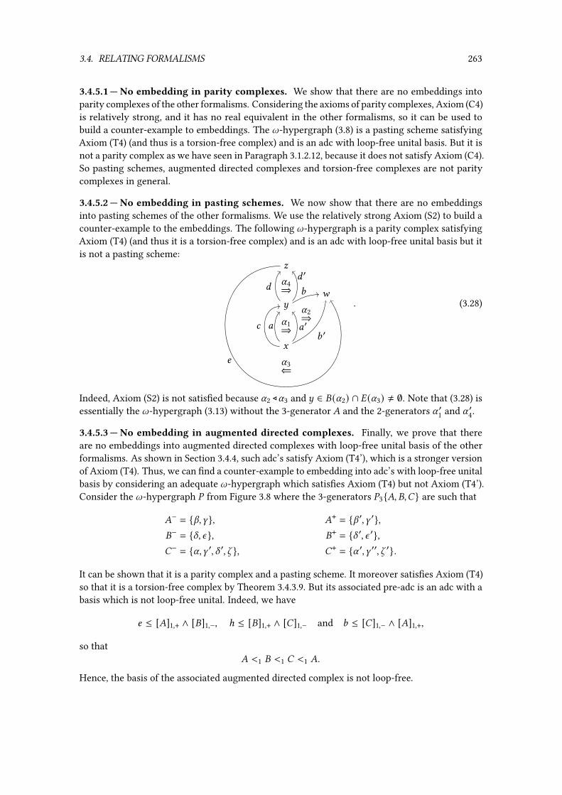
3.4. RELATING FORMALISMS 263

3.4.5.1 — No embedding in parity complexes. We show that there are no embeddings intoparity complexes of the other formalisms. Considering the axioms of parity complexes, Axiom (C4)is relatively strong, and it has no real equivalent in the other formalisms, so it can be used tobuild a counter-example to embeddings. The l-hypergraph (3.8) is a pasting scheme satisfyingAxiom (T4) (and thus is a torsion-free complex) and is an adc with loop-free unital basis. But it isnot a parity complex as we have seen in Paragraph 3.1.2.12, because it does not satisfy Axiom (C4).So pasting schemes, augmented directed complexes and torsion-free complexes are not paritycomplexes in general.

3.4.5.2 — No embedding in pasting schemes. We now show that there are no embeddingsinto pasting schemes of the other formalisms. We use the relatively strong Axiom (S2) to build acounter-example to the embeddings. The following l-hypergraph is a parity complex satisfyingAxiom (T4) (and thus it is a torsion-free complex) and is an adc with loop-free unital basis but itis not a pasting scheme:

I

~

G

F

3 ′

3

0′02

1

1 ′

4

U1⇒

U4⇒

U2⇒

U3⇐

. (3.28)

Indeed, Axiom (S2) is not satis�ed because U2 ⊳U3 and ~ ∈ �(U2) ∩ � (U3) ≠ ∅. Note that (3.28) isessentially the l-hypergraph (3.13) without the 3-generator � and the 2-generators U ′1 and U ′4.

3.4.5.3 — No embedding in augmented directed complexes. Finally, we prove that thereare no embeddings into augmented directed complexes with loop-free unital basis of the otherformalisms. As shown in Section 3.4.4, such adc’s satisfy Axiom (T4’), which is a stronger versionof Axiom (T4). Thus, we can �nd a counter-example to embedding into adc’s with loop-free unitalbasis by considering an adequate l-hypergraph which satis�es Axiom (T4) but not Axiom (T4’).Consider the l-hypergraph % from Figure 3.8 where the 3-generators %3{�, �,�} are such that

�− = {V,W}, �+ = {V ′, W ′},�− = {X, n}, �+ = {X ′, n ′},�− = {U,W ′, X ′, Z }, �+ = {U ′, W ′′, Z ′}.

It can be shown that it is a parity complex and a pasting scheme. It moreover satis�es Axiom (T4)so that it is a torsion-free complex by Theorem 3.4.3.9. But its associated pre-adc is an adc with abasis which is not loop-free unital. Indeed, we have

4 ≤ [�]1,+ ∧ [�]1,−, ℎ ≤ [�]1,+ ∧ [�]1,− and 1 ≤ [�]1,− ∧ [�]1,+,

so that� <1 � <1 � <1 �.

Hence, the basis of the associated augmented directed complex is not loop-free.

264 CHAPTER 3. PASTING DIAGRAMS

F G ~ I1

0

2

U ⇓

V ⇓4

3

5

W ⇓

X ⇓

6

ℎ

8

n ⇓

Z ⇓

�

V

F G ~ I1

0

2

U ⇓

V ′ ⇓4

3

5

W ′ ⇓

X ⇓

6

ℎ

8

n ⇓

Z ⇓

�

V

F G ~ I1

0

2

U ⇓

V ′ ⇓4

3

5

W ′ ⇓

X ′ ⇓

6

ℎ

8

n ′ ⇓

Z ⇓

�

V

F G ~ I1

0

2

U ′ ⇓

V ′ ⇓

3

5

W ′′ ⇓

6

ℎ

8

n ′ ⇓

Z ′ ⇓

Figure 3.8 – The l-hypergraph %

Chapter 4

Coherence for Gray categories

Introduction

Algebraic structures, such as monoids, can be de�ned inside arbitrary categories. In order togeneralize their de�nition to higher categories, the general principle is that one should look fora coherent version of the corresponding algebraic theory: this roughly means that we shouldadd enough higher cells to our algebraic theory so that “all diagrams commute”. For instance,when generalizing the notion of monoid from monoidal categories to monoidal 2-categories,associativity and unitality are now witnessed by 2-cells, and one should add new axioms inorder to ensure their coherence: in this case, those are MacLane’s unit (1.16) and pentagon (1.17)equations, thus resulting in the notion of pseudomonoid. The fact that these are indeed enoughto make the structure coherent constitutes a reformulation of MacLane’s celebrated coherencetheorem for monoidal categories [Mac63]. In this context, a natural question is: how can wesystematically �nd those higher coherence cells?

Rewriting theory provides a satisfactory answer to this question. Namely, if we orient theaxioms of the algebraic structures of interest in order to obtain a rewriting system which issuitably behaved (con�uent and terminating), the con�uence diagrams for critical branchingsprecisely provide us with such coherence cells. This was �rst observed by Squier for monoids,�rst formulated in homological language [Squ87] and then generalized as a homotopical condi-tion [SOK94; Laf95]. These results were then extended to strict higher categories by Guiraud andMalbos [GM09; GM12; GM18] based on a notion of rewriting system adapted to this setting, whichis provided by the polygraphs for strict categories (as introduced in Section 1.4.1). In particular,their work allow to recover the coherence laws for pseudomonoids in this way.

Our aim is to generalize those techniques in order to be able to de�ne coherent algebraicstructures inweak higher categories. We actually handle here the �rst non-trivial case, which is theone of dimension 3. Namely, it is well-known that tricategories are not equivalent to strict 3-cate-gories: the “best” one can do is to show that they are equivalent to Gray categories [GPS95; Gur13],which is an intermediate structure between weak and strict 3-categories, roughly consisting in3-categories in which the exchange law is not required to hold strictly. This means that classicalrewriting techniques cannot be used out of the shelf in this context and one has to adapt thoseto Gray categories, which is the object of this chapter. It turns out that precategories o�er anice setting for rewriting, as could already be intuited from Chapters 2 and 3. Their 2-dimen-

265

266 CHAPTER 4. COHERENCE FOR GRAY CATEGORIES

sional instances, namely sesquicategories, were already advocated by Street in the context ofrewriting [Str96]. Precategories have gained quite some interest recently, by being at the core ofthe graphical proof-assistant Globular [BKV16; BV17], which allows working with several kindsof semi-strict higher categories expressed as precategories. In particular, Gray categories are3-precategories equipped with exchange 3-cells satisfying suitable axioms.

Outline. We �rst give additional results on precategories (Section 4.1), that justify their use asa computational framework for semi-strict higher categories. In particular, we show that thecells of free precategories admit a simple description as sequences of applied whiskers (that areanalogous to contexts and context classes for strict categories), which allows a simple solution tothe word problem on prepolygraphs. Then, we show how Gray categories can be presented bythe mean of precategories after recalling the de�nition of Gray categories as categories enrichedwith strict 2-categories enriched with the Gray tensor product (Section 4.2). Next, we extendthe theory of rewriting to prepolygraphs and, more speci�cally, presentations of Gray categoriesand show that the resulting theory has good properties similar to the ones of term rewritingsystems (Section 4.3). In particular, a �nite presentation of a Gray category always has a �nitenumber of critical branchings, which contrasts with the case of strict categories [Laf03; GM09;Mim14], and the computational properties of precategories enable a mechanized computation ofthose critical branchings. Then, we derive a Squier-type coherence theorem (Theorem 4.3.4.8)and show that, given a presentation where the con�uence diagrams of the critical branchings are“�lled” by coherence cells, the presented Gray category is coherent. Finally, we apply our resultsto several algebraic structures (Section 4.4), which allows us to recover known coherence resultsand �nd new ones, such as for pseudomonoids (Section 4.4.1), pseudoadjunctions (Section 4.4.2),self-dualities (Section 4.4.4) and Frobenius pseudomonoids (Section 4.4.3).

4.1 Precategories for computations and presentations

In Chapter 2, we showed that strict categories could be seen as precategories satisfying additionalequations. This fact allowed us to give a syntactical description of cells of free strict =-cate-gories in the form of sequences of applied context classes, and which is moreover amenable tocomputation. This motivates using precategories as a more general computational frameworkfor studying other semi-strict higher categories, as we will do in the following sections. In thepresent section, we give additional properties and constructions on precategories that will makethem suitable for computations and for presenting other higher categories, like Gray categories.

We �rst give a syntactic description of free precategories by adapting the description of freestrict categories given in Section 2.2. In particular, we de�ne the notion of whisker (Section 4.1.1),which is the analogue of contexts and context classes for prepolygraphs and show that the cells offree precategories can be described as sequences of applied whiskers, which implies that free pre-categories admit a simple computational representation and the word problem on prepolygraphshas a trivial solution (Section 4.1.2). Then, we introduce several notions and constructions thatwill allow us to present precategories by the mean of prepolygraphs (Section 4.1.3).

4.1.1 Whiskers

Here, we de�ne an analogue of contexts and context classes for precategories, called whiskers,and study their properties by closely following what we did in Section 2.2.2.

4.1.1.1 — De�nition. Let = ∈ N∪ {l} and� be an =-precategory. Recall the notion of type fromSection 2.2.2. For every< ∈ N= and<-type (D,D ′), we de�ne by induction on<

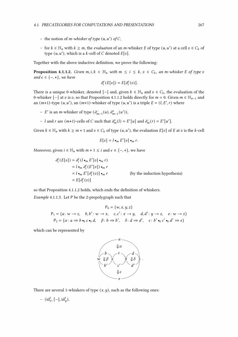
4.1. PRECATEGORIES FOR COMPUTATIONS AND PRESENTATIONS 267

– the notion of<-whisker of type (D,D ′) of � ,

– for : ∈ N= with : ≥ <, the evaluation of an<-whisker � of type (D,D ′) at a cell E ∈ �: oftype (D,D ′), which is a :-cell of � denoted � [E].

Together with the above inductive de�nition, we prove the following:

Proposition 4.1.1.2. Given <, 8, : ∈ N= with < ≤ 8 ≤ : , E ∈ �: , an <-whisker � of type Eand n ∈ {−, +}, we have

mn8 (� [E]) = � [mn8 (E)].

There is a unique 0-whisker, denoted [−] and, given : ∈ N= and E ∈ �: , the evaluation of the0-whisker [−] at E is E , so that Proposition 4.1.1.2 holds directly for< = 0. Given< ∈ N=−1 andan (<+1)-type (D,D ′), an (<+1)-whisker of type (D,D ′) is a triple � = (;, � ′, A ) where

– � ′ is an<-whisker of type (m−<−1(D), m+<−1(D ′)),

– ; and A are (<+1)-cells of � such that m+< (;) = � ′[D] and m−< (A ) = � ′[D ′].

Given : ∈ N= with : ≥ < + 1 and E ∈ �: of type (D,D ′), the evaluation � [E] of � at E is the :-cell

� [E] = ; r< � ′[E] r< A .Moreover, given 8 ∈ N= with< + 1 ≤ 8 and n ∈ {−, +}, we have

mn8 (� [E]) = mn8 (; r< � ′[E] r< A )= ; r< mn8 (� ′[E]) r< A= ; r< � ′[mn8 (E)] r< A (by the induction hypothesis)= � [mn8 (E)]

so that Proposition 4.1.1.2 holds, which ends the de�nition of whiskers.

Example 4.1.1.3. Let P be the 2-prepolygraph such that

P0 = {F, G,~, I}P1 = {0 : F → I, 1, 1 ′ : F → G, 2, 2 ′ : G → ~, 3, 3 ′ : ~ → I, 4 : F → I}P2 = {U : 0 ⇒ 1 r0 2 r0 3, V : 1 ⇒ 1 ′, X : 3 ⇒ 3 ′, n : 1 ′ r0 2 ′ r0 3 ′⇒ 4}

which can be represented by

F G ~ I

0

4

1

1 ′

2

2 ′

3

3 ′⇓V ⇓X

⇓U

⇓n

.

There are several 1-whiskers of type (G,~), such as the following ones:

– (id1G , [−], id1

~),

268 CHAPTER 4. COHERENCE FOR GRAY CATEGORIES

– (1, [−], id1~),

– (id1G , [−], 3),

– �5 ,ℎ = (5 , [−], 6) for 5 ∈ {1,1 ′} and ℎ ∈ {3, 3 ′}.

Note that, for 5 ∈ {1,1 ′} and ℎ ∈ {2, 2 ′}, the evaluation of �5 ,ℎ at 6 ∈ {2, 2 ′} is 5 r0 6 r0 ℎ. Thereare several 2-whiskers of type (2, 2 ′), as the following ones:

– �1 = (U r1 (V r0 2 r0 3) r1 (1 ′ r0 2 r0 X), �1′,3′, n),– �1 = (U r1 (1 r0 2 r0 X) r1 (V r0 2 r0 3 ′), �1′,3′, n),– �2 = (U r1 (1 r0 2 r0 X), �1,3′, (V r0 2 ′ r0 3 ′) r1 n),– �3 = (U r1 (V r0 2 r0 3), �1′,3 , (1 ′ r0 2 ′ r0 X) r1 n),– �4 = (U, �1,3 , (V r0 2 ′ r0 3) r1 (1 ′ r0 2 ′ r0 X) r1 n),– �4 = (U, �1,3 , (1 r0 2 ′ r0 X) r1 (V r0 2 ′ r0 3 ′) r1 n).

The reader is invited to compare the above whiskers with the contexts of Example 2.2.2.3.

4.1.1.4 — Source and target of whiskers. Let = ∈ N ∪ {l} and � be an =-precategory. Givenan integer< ∈ N∗= , an<-type (D,D ′) of� and an<-whisker � = (;, � , A ) of type (D,D ′), the sourceand the target of � are respectively the (<−1)-cells

m−<−1(�) = m−<−1(;) and m+<−1(�) = m+<−1(A ).When< > 1, we moreover have

mn<−2 ◦ m−<−1(�) = mn<−2 ◦ m+<−1(�)for n ∈ {−, +}. Indeed, given (; ′, � ′′, A ′) = � ′,

m+<−1(;) = ; ′ r<−2 �′′[D] r<−2 A

′ and m−<−1(A ) = ; ′ r<−2 �′′[D ′] r<−2 A

′

so that

m−<−2 ◦ m−<−1(�) = m−<−2 ◦ m−<−1(;)= m−<−2 ◦ m+<−1(;)= m−<−2(; ′)= m−<−2 ◦ m−<−1(A )= m−<−2 ◦ m+<−1(A )= m−<−2 ◦ m+<−1(�)

and similarly, m+<−2 ◦ m−<−1(�) = m+<−2 ◦ m+<−1(�). Given 8 ∈ N<−1, n ∈ {−, +}, we write mn8 (�)for mn8 ◦ mn<−1(�). With these notations, for 8 ∈ N=−1, we can extend the notion of 8-composablesequences of globes of globular sets to sequences -1, . . . , -; for some ; ∈ N∗ where -B is either awhisker or a cell of � for B ∈ N∗

;, and say that -1, . . . , -; is 8-composable when

m+8 (-B) = m−8 (-B+1) for B ∈ N∗;−1.

It is immediate that the source and target operations are compatible with the evaluation ofwhiskers:

Proposition 4.1.1.5. Given 8,<, : ∈ N= with 8 < < ≤ : , n ∈ {−, +}, a :-cell D ∈ � and an<-whisker � of type D, we have

mn8 (� [D]) = mn8 (�).

4.1. PRECATEGORIES FOR COMPUTATIONS AND PRESENTATIONS 269

4.1.1.6 — Identity whiskers. Let = ∈ N ∪ {l} and � be an =-precategory. Given< ∈ N= andan<-type (D,D ′) of � , we de�ne an<-whisker � (D,D′) , called the identity whisker on (D,D ′), byinduction on<. When< = 0, we put

� (∗,∗) = [−]and, when< > 0, we put

� (D,D′) = (id<D , � (m

−<−2 (D),m+<−2 (D′)) , id<D′)

If � is part of an =-cellular extension (�,- ) ∈ PCat+= , given 6 ∈ - , we write �6 for

� (m−=−1 (6),m+=−1 (6)) .

The identity whiskers have then trivial evaluations:

Proposition 4.1.1.7. For<,: ∈ N= with< ≤ : , an<-type (D,D ′) and E ∈ �: of type (D,D ′), wehave

� (D,D′) [E] = E .

Proof. This is shown by a simple induction on<. �

4.1.1.8 — Composition operations. Let = ∈ N ∪ {l} and � be an =-precategory. Let 8,< ∈ N=with 8 < <, (D,D ′) be an <-type and � = (;, � ′, A ) be an <-whisker of type (D,D ′). Given acell E ∈ �8+1 such that (E, �) is 8-composable, we de�ne an<-whisker E r

8 � using an inductionon< − 8 by

E r8 � =

{(E r

8 ;, �′, A ) if 8 + 1 =<,

(E r8 ;, E r

8 �′, E r

8 A ) if 8 + 1 < <.

Similarly, when (�, E) is 8-composable, we de�ne an<-whisker � r8 E using an induction on< − 8

by

� r8 E =

{(;, � ′, A r

8 E) if 8 + 1 =<,(; r8 E, � ′ r8 E, A r

8 E) if 8 + 1 < <.

These composition operations satisfy properties similar to the axioms of (=+1)-precategories:

Proposition 4.1.1.9. Given< ∈ N= , an<-type (D,D ′) of� and an<-whisker � of type (D,D ′), wehave

(i) for all 8 ∈ N<−1 and D1 = m−8 (�), D2 = m

+8 (�),

id8+1D1r8 � = � = � r

8 id8+1D2 ,

(ii) for all 8 ∈ N<−1 and D1, D2 ∈ �8+1, if D1, D2, � are 8-composable or D1, �,D2 are 8-composableor �,D1, D2 are 8-composable, then we respectively have

(D1 r8 D2) r8 � = D1 r

8 (D2 r8 �)

or

(D1 r8 �) r8 D2 = D1 r

8 (� r8 D2)

or

(� r8 D1) r8 D2 = � r

8 (D1 r8 D2),

(iii) for all 8, 9 ∈ N<−1 such that 8 < 9 , and D1, D2 ∈ �8+1 and E1, E2 ∈ � 9+1 such that D1, �,D2 are8-composable and E1, �, E2 are 9-composable, we have

D1 r8 (E1 r

9 � r9 E2) r8 D2 = (D1 r

8 E1 r8 D2) r9 (D1 r

8 � r8 D2) r9 (D1 r

8 E2 r8 D2).

270 CHAPTER 4. COHERENCE FOR GRAY CATEGORIES

Proof. By a direct adaptation of the proof of Proposition 2.2.2.11. �

Finally, we prove that the composition operations on whiskers are compatible with evaluation:

Proposition 4.1.1.10. Given 8,<, : ∈ N= with 8 < < ≤ : , D ∈ �8+1, E ∈ �: and an<-whisker � oftype E , if D, � are 8-composable, then

(D r8 �) [E] = D r

8 (� [E])

and otherwise, if �,D are 8-composable, then

(� r8 D) [E] = (� [E]) r8 D.

Proof. By a direct adaptation of the proof of Proposition 2.2.2.13. �

4.1.1.11 —Whiskers and functoriality. Let = ∈ N ∪ {l} and �, � be two =-precategories.Given an =-prefunctor � : � → � , we extend � to <-whiskers. More precisely, given < ∈ N= ,an <-type (D,D ′) of � and an <-whisker � of type (D,D ′), we de�ne an <-whisker � (�) oftype (� (D), � (D ′)) by induction on< as follows. If< = 0, we put

� ( [−]) = [−]

Otherwise, if< > 0, given (;, � ′, A ) = �, we put

� (�) = (� (;), � (� ′), � (A )).

We then have compatibility results between � and the operations on whiskers, analogous to theones shown for contexts and context classes:

Proposition 4.1.1.12. Given<,: ∈ N= with< ≤ : , D ∈ �: and an<-whisker � of type D, we have

� (� [D]) = � (�) [� (D)].

Proof. By a simple induction on<. �

Proposition 4.1.1.13. Given< ∈ N= and an<-type (D,D ′), we have � (� (D,D′) ) = � (� (D),� (D′)) .

Proof. By a simple induction on<. �

Proposition 4.1.1.14. Given 8,< ∈ N= with 8 < <,D ∈ �8+1 and an<-whisker �, ifD, � (resp. �,D)are 8-composable, then

� (D r8 �) = � (D) r8 � (�) (resp. � (� r

8 D) = � (�) r8 � (D)).Proof. By a direct adaptation of the proof of Proposition 2.2.2.17. �

4.1.2 Free precategories

Let = ∈ N. Following what was done in Section 2.2.3 and Section 2.2.4, we give a concretedescription of the functor

−[−]= : PCat+= → PCat=+1

based on whiskers. By adapting the content of Sections 2.3 and 2.4, this description allows asimple computational representation of cells of free precategories, providing a trivial solutionto the word problem. The results of this section thus advocate the use of precategories for thecomputational treatment of semi-strict higher categories like Gray categories.

4.1. PRECATEGORIES FOR COMPUTATIONS AND PRESENTATIONS 271

4.1.2.1 — Free extensions with whiskers. Let (�,- ) ∈ PCat+= be an =-cellular extension. Wewrite � [- ] for the (=+1)-globular set such that � [- ]≤= = � and � [- ]=+1 is the set of sequencesof the form

B = ((61, �1), . . . , (6: , �: ))

for some : ∈ N, called the length of B , and where68 ∈ - and �8 is an=-whisker of type68 for 8 ∈ N∗:

(when : = 0, by convention, there is an empty sequence ( )D for each D ∈ �=). The source andtarget of B as above are de�ned by

m−= (B) = �1 [d−= (61)] and m+= (B) = �: [d+= (6: )]

so that � [- ] is an (=+1)-globular set by Proposition 4.1.1.5.

We now equip � [- ] with a structure of (=+1)-precategory that extends the one of � . Given an=-cell D ∈ �= , we put

id=+1D = ( )D .

Given B = ((61, �1), . . . , (6: , �: )) ∈ � [- ]=+1 and 8 ∈ N=−1, for D ∈ �8+1 such that D, B are 8-compo-sable, we put

D r8 B = ((61, D r

8 �1), . . . , (6: , D r8 �: ))

and, similarly, for E ∈ �8+1 such that B, E are 8-composable, we put

B r8 E = ((61, �1 r

8 E), . . . , (6: , �: r8 E))

and, �nally, for B ′ = ((6′1, � ′1), . . . , (6′; , �′;)) ∈ � [- ]=+1 such that B, B ′ are =-composable, we put

B r= B′ = ((61, �1), . . . , (6: , �: ), (6′1, � ′1), . . . , (6′; , �

′;)).

We check that:

Proposition 4.1.2.2. The operations id=+1 and r8 de�ned above equip � [- ] with a structure of an

(=+1)-precategory.

Proof. The axioms of precategories are easily veri�ed using Proposition 4.1.1.9 and the fact that�is an =-precategory. �

In particular, we can use whiskers and whisker evaluations in � [- ]. We then observe that:

Lemma 4.1.2.3. Given< ∈ N= , 6 ∈ - and an<-whisker � of type 6, we have

� [(6, �6)] = (6, �↑=)

where, for : ∈ N= with : ≥ <, �↑: is the :-whisker of type 6 de�ned inductively by

�↑: =

{� if : =<,(id:

�↑:−1 [m−:−1 (6) ], �↑:−1, id:�↑:−1 [m+:−1 (6) ]

) if : > <.

In particular, if< = =, we have � [(6, �6)] = (6, �).

Proof. By a simple induction on<. �

With the above lemma, we can deduce the freeness of � [- ]:

Theorem 4.1.2.4. The (=+1)-precategory � [- ] is the free (=+1)-precategory relatively to the for-getful functorV: : PCat=+1 → PCat+= .

272 CHAPTER 4. COHERENCE FOR GRAY CATEGORIES

Proof. Let � ∈ PCat=+1 and (�, 5 ) : (�,- ) → (�≤=, �=+1) ∈ PCat+= . We de�ne a function

5 ′ : � [- ]=+1 → �=+1

by putting, for D ∈ �= ,5 ′(( )D) = id=+1

� (D)

and, for B = ((61, �1), . . . , (6: , �: )) ∈ � [- ]=+1,

5 ′(B) = � (�1) [5 (61)] r= · · · r= � (�: ) [5 (6: )]which is well-de�ned since, for 8 ∈ N∗

:−1,

m+= (� (�8) [5 (68)]) = � (�8) [m+= (5 (68))] (by Proposition 4.1.1.2)= � (�8) [� (d+= (68))]= � (�8 [d+= (68)]) (by Proposition 4.1.1.12)= � (�8+1 [d−= (68+1)])= � (�8+1) [� (d−= (68+1))] (by Proposition 4.1.1.12)= � (�8+1) [m−= (5 (68+1))]= m−= (� (�8+1) [5 (68+1)]) (by Proposition 4.1.1.2).

Moreover, a similar computation shows that, for n ∈ {−, +},

mn= (5 ′(B)) = � (�1 [d−= (61)]) = � (m−= (B))

so that (�, 5 ′) : � [- ] → � is a morphism of (=+1)-globular set. We verify that it is an (=+1)-pre-functor. By de�nition, (�, 5 ′) commutes with the identity operations. Let 8 ∈ N=−1, a cell D ∈ �8+1and B = ((61, �1), . . . , (6: , �: )) ∈ � [- ]=+1. If D, B are 8-composable, we compute that

5 ′(D r8 B) = � (D r

8 �1) [5 (61)] r= · · · r= � (D r8 �: ) [5 (6: )]

= (� (D) r8 � (�1)) [5 (61)] r= · · · r= (� (D) r8 � (�: )) [5 (6: )](by Proposition 4.1.1.14)

= (� (D) r8 � (�1) [5 (61)]) r= · · · r= (� (D) r8 � (�: ) [5 (6: )])(by Proposition 4.1.1.10)

= � (D) r8 (� (�1) [5 (61)] r= · · · r= � (�: ) [5 (6: )])= � (D) r8 5 ′(B)

and, similarly, if B,D are 8-composable, we have 5 ′(B r8 D) = 5 ′(B) r8 � (D). Thus, (�, 5 ′) is an

(=+1)-prefunctor.

The operation (�, 5 ) ↦→ (�, 5 ′) de�nes a function

Φ� : PCat+= ((�,- ), (�≤: , �=+1)) → PCat=+1(� [- ], �)

which is natural in � . It is injective since, by Propositions 4.1.1.7 and 4.1.1.13, we have

5 ′(((6, �6))) = 5 (6)

for all 6 ∈ - , and it is surjective since, by Lemma 4.1.2.3 and Proposition 4.1.1.12, a morphism

(� , 5 ) : � [- ] → � ∈ PCat=+1

is completely determined by � and the images of ((6, �6)) ∈ � [- ]=+1 by 5 for 6 ∈ - . Thus, � [- ]is the free (=+1)-precategory on (�,- ). �

4.1. PRECATEGORIES FOR COMPUTATIONS AND PRESENTATIONS 273

The above theorem gives a unique normal form property for the cells of � [- ]:

Corollary 4.1.2.5. Given D ∈ � [- ]=+1, D can be uniquely written as

D = D1 r= · · · r= D:

for some : ∈ N and D1, . . . , D: ∈ � [- ]=+1 such that, for 8 ∈ N∗:,

D8 = ;8,= r=−1 (;8,=−1 r

=−2 · · · r1 (;8,1 r0 68 r0 A8,1) r1 · · · r=−2 A8,=−1) r=−1 A8,= (4.1)

for some 68 ∈ - and ;8, 9 , A8, 9 ∈ � 9 for 9 ∈ N∗= , and the decomposition (4.1) of each D8 is moreoverunique.

Proof. By Theorem 4.1.2.4, D can be uniquely written as

D = �1 [61] r= · · · r= �: [6: ]for some : ∈ N, (=+1)-generators 61, . . . , 6: ∈ - and whiskers �1, . . . , �: . Putting D8 = �8 [68], oneobtains the decomposition (4.1) of D8 by expanding the de�nition of �8 [68]. This decompositionof D8 is unique since �8 is unique relatively to D. �

Anticipating the use of precategories for rewriting in Section 4.3, we call rewriting step an(=+1)-cell of � [- ] of the form (4.1). In the case = = 2 that will mostly concern us in the fol-lowing, a rewriting step of � [- ] is then a 3-cell ( of the form

( = _ r1 (; r0 � r0 A ) r1 dfor some ;, A ∈ �1, _, d ∈ �2 and � ∈ - .Remark 4.1.2.6. By adapting the terminology of Section 2.3.1, if the =-cellular extension (�,- )is equipped with an injective and decidable encoding E (�,- ) , one can de�ne an injective anddecidable encodings for the <-whiskers of � , by taking inspiration from Proposition 2.3.2.7(i).Then, using the standard derivation of encodings for �nite sequences (c.f. Paragraph 2.3.1.12), oneobtains an encoding of the (=+1)-cells of � [- ], and thus, an encoding E� [- ] of the (=+1)-pre-category � [- ] that extends E� . Moreover, our description of � [- ]=+1 turns into a computablefunction which takes as input a code for the =-cellular extension (�,- ), and outputs a code forthe (=+1)-precategory� [- ] and a code for the function which maps 6 ∈ - to ((6, �6)) ∈ � [- ]=+1.

4.1.2.7 — The word problem on prepolygraphs. One can consider an analogue of the wordproblem on strict polygraphs for prepolygraphs, that we shall explicitly describe. Let = ∈ N∪ {l}and P be an =-prepolygraph. For : ∈ N= , we de�ne the sets of :-terms T P

:of P inductively as

follows:

– for : ∈ N= and 6 ∈ P: , there is a :-term gen: (6) ∈ T P:,

– for : ∈ N=−1 and a :-term C ∈ T P:, there is a (:+1)-term id:+1

:(C) ∈ T P

:+1,

– for :, ;,< ∈ N∗= with< = max(:, ;), a :-term C1 ∈ T P:

and an ;-term C2 ∈ T P;, there is an

<-term C1 r:,; C2 ∈ T P

< .

Following Section 2.4, one then de�nes the set WP =⊔:∈N=WP

:of well-typed terms and an

evaluation functionÈ−ÉP : WP → P∗.

The word problem consists in, given C1, C2 ∈ WP, deciding whether ÈC1ÉP = ÈC2ÉP or not.

274 CHAPTER 4. COHERENCE FOR GRAY CATEGORIES

Remember that the key step in our description of a solution to the word problem on polygraphsof strict categories was to show that one can compute the codes of the free (=+1)-categorieson =-cellular extensions (Remark 2.3.2.36). This is rather trivial for precategories, as stated byRemark 4.1.2.6. Thus, by adapting the formalism given in Section 2.4.2, we get an implementablesolution to the word problem on prepolygraphs. More precisely, by directly adapting the no-tions of set-encoded polygraph, term de�nition of polygraphs, and of word problem instance toprepolygraphs, we get a decidable property analogous to Proposition 2.4.2.14:

Proposition 4.1.2.8. The function which takes as input an =-word problem instance (�, (C1, C2))(of prepolygraphs) and outputs 0 if ÈC1É ≠ ÈC2É, and 1 if ÈC1É = ÈC2É, is computable.

Proof. By adapting the content of Section 2.4.2 to prepolygraphs, using Remark 4.1.2.6. �

4.1.3 Presentations of precategories

In this section, we introduce the tools that we will use to present precategories, like Gray cate-gories, by the mean of prepolygraphs. First, we specify in which sense an (=+1)-prepolygraphpresent an =-precategory. Basically, the (=+1)-generators of such prepolygraph induce a relationon the =-cells of the free =-precategory that one can use to quotient those cells, and the quoti-enting operation can be simply de�ned as a left adjoint to (−)PCat

↑=+1,= . Then, since the techniqueswe develop in the next sections will target (3, 2)-Gray categories, i.e., a subset of 3-precategorieswhere each 3-cell is invertible, we moreover recall the classical localization construction in thecase of precategories. Such construction will allow us later to consider the free (3, 2)-precategoryassociated to a 3-precategory presented by the mean of a 4-prepolygraph.

4.1.3.1 — Quotienting top-level cells. Given = ∈ N∗ and an =-precategory � , a congruencefor � is an equivalence relation ∼ on �= such that, for all D,D ′ ∈ �= satisfying D ∼ D ′,

– mn=−1(D) = mn=−1(D ′) for n ∈ {−, +},

– for 8 ∈ N=−1 and E,F ∈ �8+1 such that E,D,F are 8-composable, we have

E r8 D r

8 F ∼ E r8 D′ r8 F.

Given such a congruence for� , there is an =-precategory�/∼ which is the =-precategory � suchthat �8 = �8 for 8 ∈ N=−1 and �= = �=/∼ and where the identities and compositions are inducedby the ones on � . If � = �≤= for some (=+1)-precategory � , there is a canonical congruence ∼�on � which is induced by the (=+1)-cells �=+1, i.e., ∼� is the smallest congruence on � suchthat m−= (D) ∼� m+= (D) for D ∈ �=+1. Writing �//= for �≤=/∼� , there is a quotient functor

È−É� : �≤= → �//=

often simply denoted È−É, which is the identity on �8 for 8 ∈ N=−1, and which maps D ∈ �= to itsclass ÈDÉ under ∼� . The operation � ↦→ �//= extends to a functor

(−)PCat//=,=+1 : PCat=+1 → PCat=

often simply denoted (−)PCat//= , which satis�es that:

Proposition 4.1.3.2. (−)PCat//=,=+1 is a left adjoint to (−)

PCat↑=+1,= .

4.1. PRECATEGORIES FOR COMPUTATIONS AND PRESENTATIONS 275

Proof. Let � ∈ PCat=+1 and � ∈ PCat= . Given an (=+1)-prefunctor

� : � → �↑=+1 ∈ PCat=+1,

we build an =-prefunctor � ′ : �//= → � by putting

� ′≤=−1 = �≤=−1 and � ′(ÈDÉ) = � (D) for D ∈ �= ,

and this is well-de�ned since, for E ∈ �=+1, we have

� (m−= (E)) = m−= (� (E)) = m−= (id=+1� (m−= (E)) ) = m+= (id=+1� (m−= (E)) ) = m

+= (� (E)) = � (m+= (E))

so that �= is compatible with ∼� . Moreover, � ′ is easily shown to be compatible with the structureof =-precategory, so that it is indeed an =-prefunctor.

Conversely, given an =-prefunctor

� : �//= → � ∈ PCat= ,

we build an (=+1)-prefunctor � ′ : � → �↑=+1 by putting

� ′≤= = � ◦ È−É� and � ′(E) = id=+1� (Èm−= (E)É) for E ∈ �=+1.

We now show that this de�nition is compatible with the structures of (=+1)-precategories of �and �↑=+1. Given E ∈ �=+1 and n ∈ {−, +}, we have

� ′(mn= (E)) = � (Èmn= (E)É) = � (Èm−= (E)É) = mn= (id=+1� (Èm−= (E)É) ) = mn= (� ′(E)),

and, given D ∈ �= , we have

� ′(id=+1D ) = id=+1� (Èm−= (id=+1D )É)

= id=+1� (ÈDÉ) .

Moreover, given 8 ∈ N= , E1 ∈ �8+1 and E2 ∈ �=+1 such that E1, E2 are 8-composable, if 8 < =, then

� ′(E1 r8 E2) = id=+1

� (Èm−= (E1 q8E2)É) = E1 r8 id=+1

� (Èm−= (E2)É) = E1 r8 �′(E2)

and, if 8 = =, then

� ′(E1 r= E2) = id=+1

� (Èm−= (E1 q=E2)É)

= id=+1� (Èm−= (E1)É)

= id=+1� (Èm−= (E1)É)

r= id=+1

� (Èm−= (E1)É)

= id=+1� (Èm−= (E1)É)

r= id=+1

� (Èm+= (E1)É) (by de�nition of ∼� )

= id=+1� (Èm−= (E1)É)

r= id=+1

� (Èm−= (E2)É)

= � ′(E1) r= � ′(E2)

and similarly for 8-composable E1 ∈ �=+1 and E2 ∈ �8+1. Thus, � ′ is an (=+1)-prefunctor.

The operations � ↦→ � ′ and � ↦→ � ′ are easily proved to be inverse of each other, so that we geta bijection

Ψ�,� : PCat=+1(�, �↑=+1) → PCat= (�//=, �)

which is natural in � and � . Thus, (−)PCat//=,=+1 is a left adjoint to (−)PCat

↑=+1,= . �

276 CHAPTER 4. COHERENCE FOR GRAY CATEGORIES

4.1.3.3 — Presenting with prepolygraphs. Given = ∈ N, the quotienting operation de�ned isthe previous paragraph naturally de�nes a notion of presentation of =-categories by (=+1)-pre-polygraphs. Consider the functor (−) : Pol=+1 → PCat= de�ned as the composite

Pol=+1 PCat=+1 PCat=(−)∗,=+1 (−)PCat

//=

which, to an (=+1)-prepolygraph P, associates the =-precategory P = P∗/∼P∗ . By the de�nitionof ∼P∗ and the description of −[−]= given in Section 4.1.2, we have that ∼P∗ is the smallestcongruence on P∗ such that d−= (6) ∼P

∗ d+= (6) for 6 ∈ P=+1, so that we often simply write ∼P for ∼P∗ .In the following, we say that an (=+1)-prepolygraph P is a presentation of an =-precategory �when � is isomorphic to P.

4.1.3.4 — (3, 2)-precategories. We now recall the classical localization construction in the caseof precategories, that will allow us later to consider (3, 2)-precategories presented by 4-prepoly-graphs.

Given a 3-precategory � , a 3-cell � : q V q ′ ∈ �3 is invertible when there exists � : q ′ V q suchthat � r2 � = id

qand � r2 � = id

q′ . In this case, � is unique and we write �−1 for � . A (3, 2)-pre-category is a 3-precategory where every 3-cell is invertible. The (3, 2)-precategories form a fullsubcategory of PCat3 denoted PCat(3,2) . There is a forgetful functor

U : PCat(3,2) → PCat3

which admits a left adjoint (−)> also called localization functor described as follows. Given a3-precategory � , for every � : q ⇒ q ′ ∈ �3, we write �+ for a formal element of source q andtarget q ′, and �− for a formal element of source q ′ and target q . A zigzag of � is a list

(�n11 , . . . , �

n::) (4.2)

for some : ∈ N, �1, . . . , �: ∈ �3 and n1, . . . , n: ∈ {−, +} such that

m+2 (�n88) = m−2 (�

n8+18+1 ) for 8 ∈ N∗

:−1

where we use the convention that there is one empty list ( )q for each q ∈ P∗2. The source and thetarget of a zigzag as in (4.2) are m−2 (�

n11 ) and m+2 (�

n::) respectively. Then, we de�ne a 3-globular

set�> such that (�>)≤2 = �≤2 and�>3 is the quotient of the zigzags de�ned above by the followingequalities: for every zigzag (�n1

1 , . . . , �n::),

– if �8 = id3k

for some 8 ∈ N∗:

andk ∈ �2, then

(�n11 , . . . , �

n::) = (�n1

1 , . . . , �n8−18−1 , �

n8+18+1 , . . . , �

n::),

– if n8 = n8+1 = + for some 8 ∈ N∗:−1, then

(�n11 , . . . , �

n::) = (�n1

1 , . . . , �n8−18−1 , (�8 r2 �8+1)+, �n8+28+2 , . . . , �

n::),

– if n8 = n8+1 = − for some 8 ∈ N∗:−1, then

(�n11 , . . . , �

n::) = (�n1

1 , . . . , �n8−18−1 , (�8+1 r2 �8)−, �n8+28+2 , . . . , �

n::),

– if {n8 , n8+1} = {−, +} and �8 = �8+1 for some 8 ∈ N∗:−1, then

(�n11 , . . . , �

n::) = (�n1

1 , . . . , �n8−18−1 , �

n8+28+2 , . . . , �

n::) .

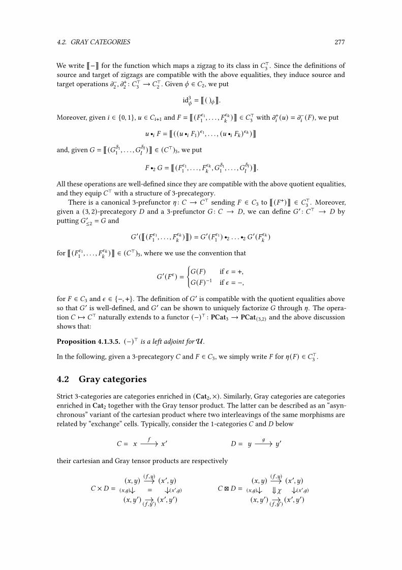
4.2. GRAY CATEGORIES 277

We write È−É for the function which maps a zigzag to its class in �>3 . Since the de�nitions ofsource and target of zigzags are compatible with the above equalities, they induce source andtarget operations m−2 , m

+2 : �>3 → �>2 . Given q ∈ �2, we put

id3q= È( )qÉ.

Moreover, given 8 ∈ {0, 1}, D ∈ �8+1 and � = È(�n11 , . . . , �

n::)É ∈ �>3 with m+8 (D) = m−8 (� ), we put

D r8 � = È((D r

8 �1)n1, . . . , (D r8 �: )n: )É

and, given � = È(�X11 , . . . ,�

X;;)É ∈ (�>)3, we put

� r2 � = È(�n11 , . . . , �

n::,�

X11 , . . . ,�

X;;)É.

All these operations are well-de�ned since they are compatible with the above quotient equalities,and they equip �> with a structure of 3-precategory.

There is a canonical 3-prefunctor [ : � → �> sending � ∈ �3 to È(�+)É ∈ �>3 . Moreover,given a (3, 2)-precategory � and a 3-prefunctor � : � → � , we can de�ne � ′ : �> → � byputting � ′≤2 = � and

� ′(È(�n11 , . . . , �

n::)É) = � ′(�n1

1 ) r2 . . . r2 � ′(�n:: )for È(�n1

1 , . . . , �n::)É ∈ (�>)3, where we use the convention that

� ′(�n ) ={� (� ) if n = +,� (� )−1 if n = −,

for � ∈ �3 and n ∈ {−, +}. The de�nition of � ′ is compatible with the quotient equalities aboveso that � ′ is well-de�ned, and � ′ can be shown to uniquely factorize � through [. The opera-tion � ↦→ �> naturally extends to a functor (−)> : PCat3 → PCat(3,2) and the above discussionshows that:

Proposition 4.1.3.5. (−)> is a left adjoint forU.

In the following, given a 3-precategory � and � ∈ �3, we simply write � for [ (� ) ∈ �>3 .

4.2 Gray categories

Strict 3-categories are categories enriched in (Cat2,×). Similarly, Gray categories are categoriesenriched in Cat2 together with the Gray tensor product. The latter can be described as an “asyn-chronous” variant of the cartesian product where two interleavings of the same morphisms arerelated by “exchange” cells. Typically, consider the 1-categories � and � below

� = G G ′5

� = ~ ~ ′6

their cartesian and Gray tensor products are respectively

� × � =(G,~) (G ′, ~)

(G,~ ′) (G ′, ~ ′)

(5 ,~)

(G,6) = (G′,6)

(5 ,~′)

� � � =(G,~) (G ′, ~)

(G,~ ′) (G ′, ~ ′)

(5 ,~)

(G,6) ⇓ j (G′,6)

(5 ,~′)

278 CHAPTER 4. COHERENCE FOR GRAY CATEGORIES

where the exchange 2-cell j can be invertible or not, depending on whether we consider thepseudo or lax variant of the Gray tensor product. We �rst recall those two variants of the Graytensor product (Section 4.2.1). We then give a more explicit description of Gray categories in termsof generators and relations (Section 4.2.2). Then, we introduce an economical way to describethe structure of a Gray category with Gray presentations (Section 4.2.3), and show that the lattercorrectly present Gray categories (Section 4.2.4).

4.2.1 The Gray tensor products

We recall here the de�nitions of the lax and pseudo variants of the Gray tensor products, that areboth tensor products on the category of strict 2-categories Cat2. We refer the reader to [Gra06,Section I, 4] for details.

4.2.1.1 — The lax Gray tensor product. In the following, we consider the 2-precategoricalsyntax for strict 2-categories, as given by Theorem 1.4.3.8. By the condition (E), a strict 2-categoryis then simply a 2-precategory � such that, for all 0-composable q,k ∈ �2,

(q r0 m−1 (k )) r0 (m+1 (q) r0 k ) = (m−1 (q) r0 k ) r0 (q r0 m+1 (k )) .Given two strict 2-categories �, � ∈ Cat2, we de�ne another strict 2-category � �lax � which ispresented as follows:

– the 0-cells of � �lax � are the pairs (G,~) where G ∈ �0 and ~ ∈ �0,

– the 1-cells of � �lax � are generated by the 1-cells

(5 , ~) : (G,~) → (G ′, ~) and (G, 6) : (G,~) → (G,~ ′),

for 5 : G → G ′ ∈ �1 and 6 : ~ → ~ ′ ∈ �2,

– the 2-cells of � �lax � are generated by the 2-cells

(q,~) : (5 , ~) → (5 ′, ~) and (G,k ) : (G, 6) → (G, 6′)

for G,~ ∈ �0, q : 5 ⇒ 5 ′ ∈ �2 andk : 6⇒ 6′ ∈ �2, and by the 2-cells

(G,~) (G ′, ~)

(G,~ ′) (G ′, ~ ′)

(G,6)

(5 ,~)

⇓ (5 , 6) (G′,6)

(5 ,~′)

for 5 : G → G ′ ∈ �1 and 6 : ~ → ~ ′ ∈ �1,

under the conditions that

(i) the 1-generators are compatible with 0-composition, meaning that

(id1G , ~) = (G, id1

~) = id1(G,~)

(5 r0 5 ′, ~) = (5 , ~) r0 (5 ′, ~)(G,6 r0 6′) = (G, 6) r0 (G,6′)

for all G ∈ �0, ~ ∈ �0, 0-composable 5 , 5 ′ ∈ �1 and 0-composable 6,6′ ∈ �1,

4.2. GRAY CATEGORIES 279

(ii) the 2-generators are compatible with 0-composition, meaning that

(id2G , ~) = (G, id2

~) = id2(G,~)

(q1 r0 q2, ~) = (q1, ~) r0 (q2, ~)(G,k1 r0 k2) = (G,k1) r0 (G,k2)

for all G ∈ �0,~ ∈ �0, 0-composableq, q ′ ∈ �2 and 0-composablek,k ′ ∈ �2, i.e., graphically,

(G,~) (G,~)

(id1G ,~)

(id1G ,~)

⇓ (id2G , ~) = (G,~) (G,~)

(G,id1~ )

(G,id1~ )

⇓ (G, id2~) = (G,~) (G,~)

id1(G,~)

id1(G,~)

⇓ id2(G,~)

(G0, ~) (G2, ~)

(51 q0 52,~)(5 ′1 q0 5 ′2 ,~)⇓(q1 r0q2, ~) = (G0, ~) (G1, ~) (G2, ~)

(51,~)

(5 ′1 ,~)

⇓(q1, ~)

(52,~)

(5 ′2 ,~)

⇓(q2, ~)

(G,~0) (G,~2)

(G,61 q062)

(G,6′1 q06′2)⇓(G,k1 r0k2) = (G,~0) (G,~1) (G,~2)

(G,61)

(G,6′1)

⇓(G,k1)

(G,62)

(G,6′2)

⇓(G,k2) ,

(iii) the 2-generators are compatible with 1-composition, meaning that

(id25, ~) = id2

(5 ,~)

(q1 r1 q2, ~) = (q1, ~) r1 (q2, ~)(G, id2

6) = id2(G,6)

(G,k1 r1 k2) = (G,k1) r1 (G,k2)

for parallel 50, 51, 52 ∈ �1 and parallel 60, 61, 62 ∈ �1 and 2-cells

q8 : 58−1 ⇒ 58 : G → G ′ ∈ �2 and k8 : 68−1 ⇒ 68 : ~ → ~ ′ ∈ �2

for 8 ∈ {1, 2}, and 1-cells 5 : G → G ′ ∈ �1 and 6 : ~ → ~ ′ ∈ �1, i.e., graphically,

(G,~) (G ′, ~)

(5 ,~)

(5 ,~)

⇓ (id25, ~) = (G,~) (G ′, ~)

(5 ,~)

(5 ,~)

⇓ id2(5 ,~)

(G,~) (G ′, ~)

(50,~)

(52,~)

⇓ (q1 r1q2, ~) = (G,~) (G ′, ~)(51,~)

(50,~)

(52,~)

⇓ (q1, ~)

⇓ (q2, ~)

280 CHAPTER 4. COHERENCE FOR GRAY CATEGORIES

(G,~) (G,~ ′)

(G,6)

(G,6)

⇓ (G, id26) = (G,~) (G,~ ′)

(G,6)

(G,6)

⇓ id2(G,6)

(G,~) (G,~ ′)

(G,60)

(G,62)

⇓ (G,k1 r1k2) = (G,~) (G ′, ~)(G,61)

(G,60)

(G,62)

⇓ (G,k1)

⇓ (G,k2),

(iv) the interchangers are compatible with 0-composition, meaning that

(id1G , 6) = id2

(G,6)

(51 r0 52, 6) = ((51, ~) r0 (52, 6)) r1 ((51, 6) r0 (52, ~ ′))(5 , id1

~) = id2(5 ,~)

(5 , 61 r0 62) = ((5 , 61) r0 (G ′, 62)) r1 ((G, 61) r0 (5 , 62))

for all 58 : G8−1 → G8 and 68 : ~8−1 → ~8 for 8 ∈ {1, 2} and 5 : G → G ′ and 6 : ~ → ~ ′, i.e.,graphically,

(G,~) (G,~)

(G,~ ′) (G,~ ′)

(id1G , 6)⇐(G,6)

(id1G ,~)

(G,6)

(id1G ,~)

=

(G,~)

(G,~ ′)

(G,6)id2(G,6)⇐

(G,6)

(G0, ~) (G2, ~)

(G0, ~′) (G2, ~

′)⇓ (51 r0 52, 6)(51 q0 52,~)

(G0,6) (G2,6)

(51 q0 52,~′)=

(G0, ~) (G1, ~) (G2, ~)

(G0, ~′) (G1, ~

′) (G2, ~′)

(G0,6)

(51,~)

⇓ (51, 6) (G1,6)

(52,~)

⇓ (52, 6) (G2,6)

(51,~′) (52,~′)

(G,~) (G ′, ~)

(G,~) (G ′, ~)⇓ (5 , id1

~)(G,id1~)

(5 ,~)

(G′,id1~)

(5 ,~)

= (G,~) (G ′, ~)

(5 ,~)

⇓ id2(5 ,~)

(5 ,~)

(G,~0) (G ′, ~0)

(G,~2) (G ′, ~2)(G,61 q062)

(5 ,~0)

⇓ (5 , 61 r062) (G′,61 q062)

(5 ,~2)

=

(G,~0) (G ′, ~0)

(G,~1) (G ′, ~1)

(G,~2) (G ′, ~2)

(5 ,~0)

(G,61) ⇓ (5 , 61) (G′,61)

(5 ,~1)

(G,62) ⇓ (5 , 62) (G′,62)

(5 ,~2)

,

(v) the interchangers commute with the 2-generators, meaning that

((5 , 6) r1 ((G, 6) r0 (q,~ ′))) = (((q,~) r0 (G ′, 6)) r1 (5 ′, 6))((5 , 6) r1 ((G,k ) r0 (5 , ~ ′))) = (((5 , ~) r0 (G ′,k )) r1 (5 , 6′))

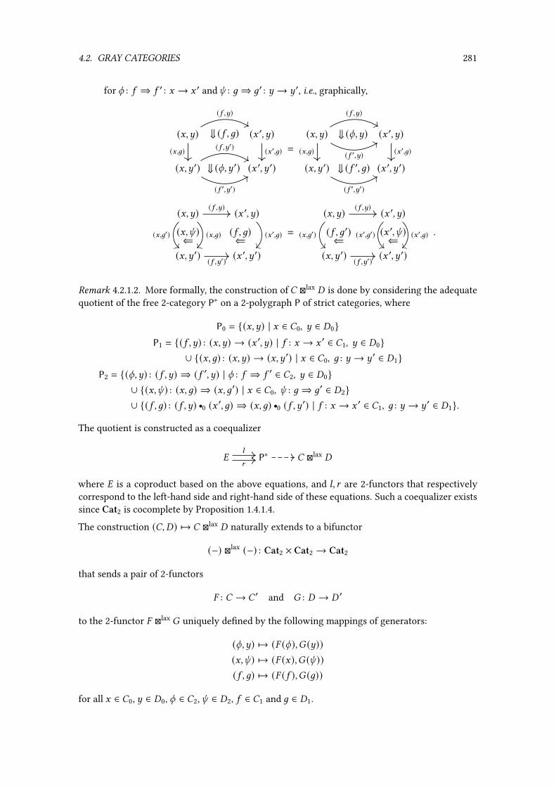
4.2. GRAY CATEGORIES 281

for q : 5 ⇒ 5 ′ : G → G ′ andk : 6⇒ 6′ : ~ → ~ ′, i.e., graphically,

(G,~) (G ′, ~)

(G,~ ′) (G ′, ~ ′)(G,6)

(5 ,~)

(G′,6)(5 ,~′)

⇓ (q,~ ′)

(5 ′,~′)

⇓ (5 , 6)=

(G,~) (G ′, ~)

(G,~ ′) (G ′, ~ ′)

⇓ (q,~)(G,6)

(5 ,~)

(5 ′,~) (G′,6)

(5 ′,~′)

⇓ (5 ′, 6)

(G,~) (G ′, ~)

(G,~ ′) (G ′, ~ ′)

(G,k )⇐(G,6′)

(5 ,~)

(G,6) (G′,6)

(5 ,~′)

(5 , 6)⇐

=

(G,~) (G ′, ~)

(G,~ ′) (G ′, ~ ′)

(G,6′)

(5 ,~)

(G′,6)(G′,6′) (G ′,k )⇐

(5 ,~′)

(5 , 6′)⇐

.

Remark 4.2.1.2. More formally, the construction of � �lax � is done by considering the adequatequotient of the free 2-category P∗ on a 2-polygraph P of strict categories, where

P0 = {(G,~) | G ∈ �0, ~ ∈ �0}P1 = {(5 , ~) : (G,~) → (G ′, ~) | 5 : G → G ′ ∈ �1, ~ ∈ �0}

∪ {(G, 6) : (G,~) → (G,~ ′) | G ∈ �0, 6 : ~ → ~ ′ ∈ �1}P2 = {(q,~) : (5 , ~) ⇒ (5 ′, ~) | q : 5 ⇒ 5 ′ ∈ �2, ~ ∈ �0}

∪ {(G,k ) : (G, 6) ⇒ (G,6′) | G ∈ �0, k : 6⇒ 6′ ∈ �2}∪ {(5 , 6) : (5 , ~) r0 (G ′, 6) ⇒ (G, 6) r0 (5 , ~ ′) | 5 : G → G ′ ∈ �1, 6 : ~ → ~ ′ ∈ �1}.

The quotient is constructed as a coequalizer

� P∗ � �lax �;

A

where � is a coproduct based on the above equations, and ;, A are 2-functors that respectivelycorrespond to the left-hand side and right-hand side of these equations. Such a coequalizer existssince Cat2 is cocomplete by Proposition 1.4.1.4.

The construction (�, �) ↦→ � �lax � naturally extends to a bifunctor

(−) �lax (−) : Cat2 × Cat2 → Cat2

that sends a pair of 2-functors

� : � → � ′ and � : � → � ′

to the 2-functor � �lax � uniquely de�ned by the following mappings of generators:

(q,~) ↦→ (� (q),� (~))(G,k ) ↦→ (� (G),� (k ))(5 , 6) ↦→ (� (5 ),� (6))

for all G ∈ �0, ~ ∈ �0, q ∈ �2,k ∈ �2, 5 ∈ �1 and 6 ∈ �1.

282 CHAPTER 4. COHERENCE FOR GRAY CATEGORIES

Writting 1 for the terminal strict 2-category whose only 0-cell is denoted ∗, for � ∈ Cat2, thereare a 2-functors

_lax� : 1 �lax � → � and d lax

� : � �lax 1→ �

uniquely de�ned by the mappings

_lax� ((∗,k )) = k and d lax

� ((k, ∗)) = k

fork ∈ �2, and both are isomorphisms natural in � .

For �, �, � ∈ Cat2, there is a 2-functor

U lax�,�,� : (� �lax �) �lax � → � �lax (� �lax �)

uniquely de�ned by the following mappings on generators

((q,~), I) ↦→ (q, (~, I)) ((5 , 6), I) ↦→ (5 , (6, I))((G, j), I) ↦→ (G, (j, I)) ((5 , ~), ℎ) ↦→ (G, (6, ℎ))((G,~),k ) ↦→ (G, (~,k )) ((G, 6), ℎ) ↦→ (G, (6, ℎ))

for G ∈ �0, ~ ∈ �0, I ∈ �0, 5 ∈ �1, 6 ∈ �1, ℎ ∈ �1, q ∈ �2, j ∈ �2,k ∈ �2, and U lax�,�,�

is moreoveran isomorphism natural in �, �, �.

By checking coherence conditions (1.16) and (1.17) of monoidal categories (c.f. Paragraph 1.5.1.1),one can verify that:

Proposition 4.2.1.3. (Cat2, 1,�lax, _lax, d lax, U lax) is a monoidal category.

The monoidal structure (Cat2, 1,�lax, _lax, d lax, U lax) is called the lax Gray tensor product.

4.2.1.4 — The pseudo Gray tensor product. The other variant of Gray tensor is called thepseudo Gray tensor product and is the monoidal structure (Cat2, 1,�, _, d, U) such that, given two2-categories �, � ∈ Cat2, � � � is de�ned the same way as � �lax � , except that we moreoverrequire that, for 5 : G → G ′ ∈ �1 and 6 : ~ → ~ ′ ∈ �1, the 2-cell (5 , 6) of � � � be invertiblefor r1. The natural isomorphisms _, d, U are then uniquely de�ned by similar mappings thanthose de�ning _lax, d lax, U lax. By checking the coherence conditions (1.16) and (1.17) of monoidalcategories, one can verify that:

Proposition 4.2.1.5. (Cat2, 1,�, _, d, U) is a monoidal category.

Remark 4.2.1.6. More formally, given �, � ∈ Cat2, � � � is built by adapting the construction ofRemark 4.2.1.2: the strict 2-category � � � is the quotient of the free 2-category Q∗ where Q isthe 2-polygraph of strict categories such that

Q0 = P0 Q1 = P1

Q2 = P2 ∪ {(5 , 6)−1 : (G, 6) r0 (5 , ~ ′) ⇒ (5 , ~) r0 (G ′, 6) | 5 : G → G ′ ∈ �1, 6 : ~ → ~ ′ ∈ �1}

Like for� �lax � , the strict 2-category� �� is then obtained by quotienting Q∗ by the mean of acoequalizer derived from the equations (i) to (v) and moreover the ones of the following additionalcondition:

(vi) for 5 : G → G ′ ∈ �1 and 6 : ~ → ~ ′ ∈ �1,

(5 , 6) r1 (5 , 6)−1 = id2((5 , ~) r0 (G ′, 6)) and (5 , 6)−1 r1 (5 , 6) = id2((G, 6) r0 (5 , ~ ′)).

4.2. GRAY CATEGORIES 283

4.2.2 Gray categories

To each of the two Gray tensor products that we de�ned in the previous section, there is anassociated notion of 3-category, that is a category enriched in Cat2 equipped with one of the twotensor products (c.f. Paragraph 1.5.1.4 for the de�nition of enriched categories). We describe thetwo notions of 3-categories, namely lax Gray categories and pseudo Gray categories. We moreoverintroduce (3, 2)-Gray categories, which are lax Gray categories where every 3-cell is invertible,that we will study in the following sections.

4.2.2.1 — Lax Gray categories. A lax Gray category (as in [Gra06, Section I, 4.25]) is a categoryenriched in the category Cat2 of strict 2-categories equipped with the lax Gray tensor product.Alternatively, we give a more explicit de�nition using generators and relations: a Gray categoryis a 3-precategory � together with, for every pair of 0-composable 2-cells

q : 5 ⇒ 5 ′ : G → ~ and k : 6⇒ 6′ : ~ → I

of � , a 3-cell

-q,k : (q r0 6) r1 (5 ′ r0 k ) V (5 r0 k ) r1 (q r0 6′)called interchanger, which can be represented using string diagrams by

5 6

q

k

5 ′ 6′

V

5 6

q

k

5 ′ 6′

and satisfying the following sets of axioms

(G-i) (compatibility with compositions and identities) given 2-cells

q : 5 ⇒ 5 ′ q ′ : 5 ′⇒ 5 ′′ k : 6⇒ 6′ k ′ : 6′⇒ 6′′

of � and 1-cells 4, ℎ of � such that 4, q,k, ℎ are 0-composable, we have

-id25,k = id3

5 q0k -q q1q′,k = ((q r0 6) r1 -q′,k ) r2 (-q,k r1 (q ′ r0 6′))-q,id2

6= id3

q q06 -q,k q1k ′ = (-q,k r1 (5 ′ r0 k ′)) r2 ((5 r0 k ) r1 -q,k ′)and

-4 q0q,k = 4 r0 -q,k -q,k q0ℎ = -q,k r0 ℎ.Moreover, given q,k ∈ �2 and 5 ∈ �1 such that q, 5 ,k are 0-composable, we have

-q q0 5 ,k = -q,5 q0k ,

(G-ii) (exchange law for 3-cells) given 3-cells

� : q V k ∈ �3 � : k V k ′ ∈ �3

of � such that �, � are 1-composable, we have

(� r1 k ) r2 (q ′ r1 �) = (q r1 �) r2 (� r1 k ′),

284 CHAPTER 4. COHERENCE FOR GRAY CATEGORIES

(G-iii) (compatibility between interchangers and 3-cells) given 3-cells

� : q V q ′ : D ⇒ D ′ and � : k ⇒ k ′ : E ⇒ E ′

of � such that �, � are 0-composable, we have

((� r0 E) r1 (D ′ r0 k )) r2 -q′,k = -q,k r2 ((D r0 k ) r1 (� r0 E ′))((q r0 E) r1 (D ′ r0 �)) r2 -q,k ′ = -q,k r2 ((D r0 �) r1 (q r0 E ′)) .

A morphism between two lax Gray categories � and � is a 3-prefunctor � : � → � such that

� (-q,k ) = -� (q),� (k )

for 0-composable q,k ∈ �2.

4.2.2.2 — Pseudo Gray categories. We similarly have a notion of pseudo Gray category which isa category enriched in the category of 2-categories equipped with the pseudo Gray tensor product.In terms of generators and relations, a pseudo Gray category is a lax Gray category� where -q,kis invertible for 0-composable q,k ∈ �2. A morphism between two pseudo Gray categories �, �is a morphism of lax Gray categories between � and � .

4.2.2.3 — (3, 2)-Gray category. A (3, 2)-Gray category is a lax Gray category whose underlying3-precategory is a (3, 2)-precategory. Note that it is then also a pseudo Gray category. As onecan expect, a localization of a lax Gray category gives a (3, 2)-Gray category:

Proposition 4.2.2.4. If � is a lax Gray category, then �> is a (3, 2)-Gray category.

Proof. Given 1-composable � : q V q ′,� : k V k ′ ∈ �3, by the exchange law for 3-cells, we have,in �>3 ,

(� r1 k ) r2 (q ′ r1 �) = (q r1 �) r2 (� r1 k ′) .By inverting � r1 k and � r1 k ′, we obtain

(q ′ r1 �) r2 (�−1 r1 k ′) = (�−1 r1 k ) r2 (q r1 �) .Similarly,

(q r1 �−1) r2 (� r1 k ) = (� r1 k ′) r2 (q ′ r1 �−1)

and(�−1 r1 k ′) r2 (q r1 �−1) = (q ′ r1 �−1) r2 (�−1 r1 k ).

Now, given general 1-composable � : q V q ′,� : k V k ′ ∈ �>3 , we have that

� = �1 r2 �−12

r2 · · · r2 �2:−1 r2 �−12:

and� = �1 r2 �−1

2r2 · · · r2 �2;−1 r2 �−1

2;

for some :, ; ∈ N∗ and �8 ,� 9 ∈ �3 for 8 ∈ N∗2: and 9 ∈ N∗2; . By applying the formulas above 4:;times to exchange the �8 ’s with the � 9 ’s, we get

(� r1 k ) r2 (q ′ r1 �) = (q r1 �) r2 (� r1 k ′) .A similar argument gives the compatibility between interchangers and 3-cells of �>. Thus, �> isa (3, 2)-Gray category. �

4.2. GRAY CATEGORIES 285

4.2.3 Gray presentations

Starting from a 3-prepolygraph P such as the one of Example 1.4.2.12 on page 69, we want toadd 3-generators to P and relations on the 3-cells of P∗3 so that we obtain a presentation of alax Gray category. This can of course be achieved naively by adding, for each pair of 0-compo-sable 2-cells q,k in P∗2, a 3-generator corresponding to the interchanger “-q,k ”, together withthe relevant relations, but the resulting presentation has numerous generators. We detail belowa more economical way of proceeding in order to present lax Gray categories. The proof thatour notion of presentation of Gray category really induces a Gray category is given in the nextsection.

4.2.3.1 — High-level de�nition. We give here the high-level de�nition of Gray presentationsand defer some technicalities to the next paragraph. A Gray presentation is a 4-prepolygraph Pcontaining the following distinguished generators:

(i) for 0-composable U,6, V with U, V ∈ P2, 6 ∈ P∗1, a 3-generator -U,6,V ∈ P3 called interchangegenerator, which is of type

-U,6,V : (U r0 6 r0 ℎ) r1 (5 ′ r0 6 r0 V) V (5 r0 6 r0 V) r1 (U r0 6 r0 ℎ′)which can be represented using string diagrams by

U

V

· · ·

· · ·

· · ·

· · ·

· · ·

· · ·

5

5 ′

6

6

ℎ

ℎ′

V

U

V

· · ·

· · ·

· · ·

· · ·

· · ·

· · ·

5

5 ′

6

6

ℎ

ℎ′

,

(ii) for every pair of 3-generators �, � ∈ P3 and 4, 4 ′, ℎ, ℎ′ ∈ P∗1 and j ∈ P∗2 as in

G ~

F I

G ′ ~ ′

5

q ⇓�V⇓q ′

6 ℎ4

⇓ j4′

5 ′

k ⇓�V⇓k ′

6′

ℎ′

(4.3)

a 4-generator of type Γ Δ, called independence generator, where

Γ = ((4 r0 � r0 ℎ) r1 j r1 (4 ′ r0 k r0 ℎ′)) r2 ((4 r0 q ′ r0 ℎ) r1 j r1 (4 ′ r0 � r0 ℎ′))and

Δ = ((4 r0 q r0 ℎ) r1 j r1 (4 ′ r0 � r0 ℎ′)) r2 ((4 r0 � r0 ℎ) r1 j r1 (4 ′ r0 k ′ r0 ℎ′)),

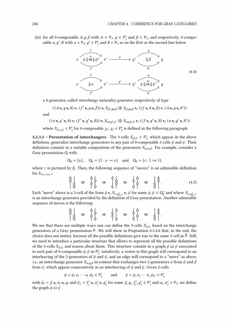
286 CHAPTER 4. COHERENCE FOR GRAY CATEGORIES

(iii) for all 0-composable �,6, V with � ∈ P3, 6 ∈ P∗1 and V ∈ P2, and respectively, 0-compo-sable U,6′, � with U ∈ P2, 6′ ∈ P∗1 and � ∈ P3 as on the �rst or the second line below

G G ′ ~ ′ ~q ⇓�V⇓q ′

5

5 ′

6 ⇓V

ℎ

ℎ′

G G ′ ~ ′ ~⇓U

5

5 ′

6′k ⇓

�V⇓k ′ℎ

ℎ′

(4.4)

a 4-generator, called interchange naturality generator, respectively of type

((� r0 6 r0 ℎ) r1 (5 ′ r0 6 r0 V)) r2 -q′,6 q0V -q,6 q0V r2 ((5 r0 ℎ r0 V) r1 (� r0 6 r0 ℎ′))and((U r0 6′ r0 ℎ) r1 (5 ′ r0 6′ r0 �)) r2 -U q06′,k ′ -U q06′,k r2 ((5 r0 6′ r0 �) r1 (U r0 6′ r0 ℎ′))

where -j1,j2 ∈ P∗3 for 0-composable j1, j2 ∈ P∗2 is de�ned in the following paragraph.

4.2.3.2 — Presentation of interchangers. The 3-cells -q,k ∈ P∗3, which appear in the abovede�nition, generalize interchange generators to any pair of 0-composable 2-cells q andk . Theirde�nition consists in a suitable composition of the generators -U,D,V . For example, consider aGray presentation Q with

Q0 = {G}, Q1 = {1 : G → G} and Q2 = {g : 1⇒ 1}

where g is pictured by . Then, the following sequence of “moves” is an admissible de�nitionfor -g q1g,g q1g :

V V V V . (4.5)

Each “move” above is a 3-cell of the form q r1 -g,id1G ,g

r1 k for some q,k ∈ Q∗2 and where -g,id1G ,g

is an interchange generator provided by the de�nition of Gray presentation. Another admissiblesequence of moves is the following:

V V V V .

We see that there are multiple ways one can de�ne the 3-cells -q,k based on the interchangegenerators of a Gray presentation P. We will show in Proposition 4.2.4.8 that, in the end, thechoice does not matter, because all the possible de�nitions give rise to the same 3-cell in P. Still,we need to introduce a particular structure that allows to represent all the possible de�nitionsof the 3-cells -q,k and reason about them. This structure consists in a graph q �k associatedto each pair of 0-composable q,k in P∗2: intuitively, a vertex in this graph will correspond to aninterleaving of the 2-generators of q and k , and an edge will correspond to a “move” as above,i.e., an interchange generator -U,6,V in context that exchanges two 2-generators U from q and Vfromk , which appear consecutively in an interleaving of q andk . Given 2-cells

q = q1 r1 · · · r1 q: ∈ P∗2 and k = k1 r1 · · · r1 k:′ ∈ P∗2with q8 = 58 r0 U8 r0 68 and k 9 = 5 ′9

r0 U ′9 r0 6′9 for some 58 , 68 , 5 ′9 , 6′9 ∈ P∗1 and U8 , U ′9 ∈ P2, we de�ne

the graph q �k

4.2. GRAY CATEGORIES 287

– whose vertices are the shu�es of the words l1 . . . l: and r1 . . . r:′ on the alphabet

Σq,k = {l1, . . . , l: , r1, . . . , r:′},

– whose edges are of the form XF,F′ : F l8r9F ′→ Fr9 l8F ′ for some 8 ∈ N∗:, 9 ∈ N∗

:′ and somewordsF,F ′ ∈ Σ∗

q,ksuch thatF l8r9F ′ ∈ (q �k )0.

Given 8 ∈ N: , 9 ∈ N:′ , ? ∈ N:−8+1, @ ∈ N:′−9+1 and a shu�e D of the words

l8 . . . l8+?−1 and r9 . . . r9+@−1,

we de�ne [D]8, 9q,k∈ P∗2 (or simply [D]8, 9 ) by induction on ? and @:

[D]8, 9 =

(q8 r0 m+1 (k 9 )) r1 [D ′]8+1, 9 if D = l8D ′,(m+1 (q8) r0 k 9 ) r1 [D ′]8, 9+1 if D = r9D ′,m+1 (q8) r0 m+1 (k 9 ) if D is the empty word,

where, by convention, m+1 (q0) = m−1 (q1) and m+1 (k0) = m−1 (k1). Note that the indices of [D]8, 9 areuniquely determined if D has at least an l letter and an r letter. Intuitively, the letters l8 and r9correspond to the 2-cells q8 r0 (−) and (−) r0k 9 where the 1-cells (−) are most of the time uniquelydetermined by the context, so that [D]1,1 for D ∈ (q � k )0 is an interleaving of the q8 r0 (−)and (−) r0 k 9 . Now, given XD,E : Dl8r9E → Dr9 l8E ∈ (q �k )1, we de�ne the 3-cell

[XD,E]q,k : [Dl8r9E]1,1q,k V [Dr9 l8E]1,1q,k∈ P∗3

by[XD,E]q,k = [D]1,1

q,kr1 (58 r0 -U8 ,68 q0 5 ′9 ,U′9 r0 6′9 ) r1 [E]8+1, 9+1q,k

.

We thus obtain a functor

[−]q,k : (q �k )∗ → P∗(m−1 (q) r0 m−1 (k ), m+1 (q) r0 m+1 (k ))where (q �k )∗ is the free 1-category on q �k considered as a 1-polygraph, and where [−]q,k isde�ned by the mappings

D ∈ (q �k )0 ↦→ [D]1,1q,k ∈ P∗2

XD,E ∈ (q �k )1 ↦→ [XD,E]q,k ∈ P∗3.

For example, forQ de�ned as above andq = k = g r1g , [l1l2r1r2]q,k and [l1r1l2r2]q,k are respectivelythe 2-cells of Q∗2

and

and [Xl1,r2]q,k and [Xl1r1,n ]q,k are respectively the 3-cells of Q∗3

V and V .

We write Xq,k for the path

XD1,E1r1 · · · r1 XD::′ ,E::′ ∈ (q �k )∗(l1 . . . l:r1 . . . r:′, A1 . . . r:′l1 . . . l: )

288 CHAPTER 4. COHERENCE FOR GRAY CATEGORIES

de�ned by induction by

D1 = l1 . . . l:−1 and E1 = r2 . . . r:′

and where D8+1, E8+1 are the unique words of Σ∗q,k

such that

m+0 (XD8 ,E8 ) = D8+1l?r@E8+1 with E8+1 = r@+1 . . . r:′l?+1 . . . l:

for some ?, @ ∈ N. We can �nally end the de�nition of Gray presentations by putting

-q,k = [Xq,k ]q,k .

For example, for Q de�ned as above, -g q1g,g q1g is the composite of 3-cells of Q∗3 given by (4.5).Example 4.2.3.3. We de�ne the Gray presentation of pseudomonoids as the 4-prepolygraph obtainedby extending the 3-prepolygraph for pseudomonoids P introduced in Example 1.4.2.12 on page 69.First, we add to P3 the 3-generators

-`,=,` : V -`,=,[ : V

-[,=,` : V -[,=,[ : V

for = ∈ N. Second, we de�ne P4 as a minimal set of 4-generators such that, given a con�gurationof cells of (P≤3)∗ as in (4.3), there is a corresponding independence generator in P4, and given acon�guration of cells of (P≤3)∗ as in the �rst or the second line of (4.4), there is a correspondinginterchange naturality generator in P4.

4.2.4 Correctness of Gray presentations

Until the end of this section, we suppose given a Gray presentation P. The aim of this section is toprove that our de�nition of Gray presentation is correct, i.e., that P has a structure of a lax Graycategory (Theorem 4.2.4.14). This will moreover implies that the localization of P has a structureof (3, 2)-Gray category (Corollary 4.2.4.15).Recall the de�nition of rewriting steps given in Paragraph 4.1.2.1. We start by showing the ex-change law for the 3-cells of P that we �rst prove on rewriting steps:

Lemma 4.2.4.1. Given rewriting steps '8 : q8 V q ′8 ∈ P∗3 for 8 ∈ {1, 2}, such that '1, '2 are 1-com-posable, we have, in P3,

('1 r1 q2) r2 (q ′1 r1 '2) = (q1 r1 '2) r2 ('1 r1 q ′2) .Proof. Let ;8 , A8 ∈ P1, _8 , d8 ∈ P2, �8 ∈ P3 such that '8 = _8 r0 (;8 r0 �8 r0 A8) r8 d8 for 8 ∈ {1, 2},and `8 , ` ′8 ∈ P2 such that �8 : `8 V ` ′8 for 8 ∈ {1, 2}. In P3, we have

('1 r1 q2) r2 (q ′1 r1 '2)= _1r1 [((;1 r0 �1 r0 A1) r1 d1 r1 _2 r1 (;2 r0 `2 r0 A2))r2 ((;1 r0 ` ′1 r0 A1) r1 d1 r1 _2 r1 (;2 r0 �2 r0 A2))]r1 d2 (by precategories axioms)= _1r1 [((;1 r0 `1 r0 A1) r1 d1 r1 _2 r1 (;2 r0 �2 r0 A2))r2 ((;1 r0 �1 r0 A1) r1 d1 r1 _2 r1 (;2 r0 ` ′2 r0 A2))]r1 d2 (by independence generator)

= (q1 r1 '2) r2 ('1 r1 q ′2). �

4.2. GRAY CATEGORIES 289

We can now conclude the exchange law for 3-cells:

Lemma 4.2.4.2. Given �8 : q8 V q ′8 ∈ P3 for 8 ∈ {1, 2} such that �1, �2 are 1-composable, we have,in P3,

(�1 r1 q2) r2 (q ′1 r1 �2) = (q1 r1 �2) r2 (�1 r1 q ′2) .Proof. For 8 ∈ {1, 2}, as an element of P3, �8 can be written �8 = '8,1 r2 · · · r2 '8,:8 where

'8, 9 = _8, 9 r1 (;8, 9 r0 �8, 9 r0 A8, 9 ) r1 d8, 9for some :8 ∈ N and _8, 9 , d8, 9 ∈ P2, ;8, 9 , A8, 9 ∈ P1, �8, 9 ∈ P3 for 9 ∈ N∗

:8. Note that

�1 r1 q2 = ('1,1 r1 q2) r2 · · · r2 ('1,:1r1 q2)

andq ′1 r1 �2 = (q ′1 r1 '2,1) r2 · · · r2 (q ′1 r1 '2,:2) .

Then, by using Lemma 4.2.4.1 :1:2 times to reorder the '1, 91 ’s after the '2, 92 ’s for 8 ∈ {1, 2}and 98 ∈ N∗:8 , we obtain that

(�1 r1 q2) r2 (q ′1 r1 �2) = (q1 r1 �2) r2 (�1 r1 q ′2). �

We now prove the various conditions on -−,−. First, a technical lemma:

Proposition 4.2.4.3. Given 5 ∈ P∗1, q,k ∈ P∗2 with 5 , q,k 0-composable, there is a canonicalisomorphism (5 r0 q) �k ' q �k and for all ? ∈ (q �k )∗1 , we have

[?]5 q0q,k = 5 r0 [?]q,k .Similarly, given q,k ∈ P∗2 and ℎ ∈ P∗1 with q,k, ℎ 0-composable, we have a canonical isomor-phism q � (k r0 ℎ) ' q �k and for all ? ∈ (q � (k r0 ℎ))∗1 , we have

[?]q,k q0ℎ = [?]q,k r0 ℎ.Finally, given q,k ∈ P∗2 and 6 ∈ P∗1 with q,6,k 0-composable, we have a canonical isomor-phism (q r0 6) �k ' q � (6 r0 k ) and for all ? ∈ ((q r0 6) �k )∗1 , we have

[?]q q06,k = [?]q,6 q0k .Proof. Let 5 ∈ P∗1, q,k ∈ P∗2 with 5 , q,k 0-composable, A, B ∈ N, 58 , 68 ∈ P∗1 and U8 ∈ P2 for 8 ∈ N∗A ,and 5 ′9 , 6

′9 ∈ P∗1 and U ′9 ∈ P2 for 9 ∈ N∗B such that

q = (51 r0 U1 r0 61) r1 · · · r1 (5A r0 UA r0 6A ) and k = (5 ′1 r0 U ′1 r0 6′1) r1 · · · r1 (5 ′A r0 U ′A r0 6′A ).By contemplating the de�nitions of (5 r0 q)�k and q �k , we deduce a canonical isomorphismbetween them. Under this isomorphism, we easily verify that we have [F]5 q0q,k = 5 r0 [F]q,kforF ∈ ((5 r0 q) �k )0. Now, given Dl8r9E ∈ ((5 r0 q) �k )0, we have

[XD,E]5 q0q,k = [D]5 q0q,k r1 (5 r0 58 r0 -U8 ,68 q0 59 ,U′9 r0 6 9 ) r1 [E]5 q0q,k= 5 r0 ( [D]q,k r1 (58 r0 -U8 ,68 q0 59 ,U′9 r0 6 9 ) r1 [E]q,k )= 5 r0 [XD,E]q,k .

By functoriality of [−]5 q0q,k and [−]q,k , we deduce that, for all ? ∈ (5 r0 q) �k ∗,

[?]5 q0q,k = 5 r0 [?]q,k .The two other properties are shown similarly. �

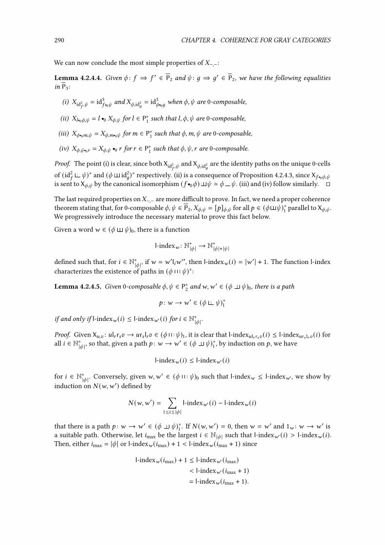
290 CHAPTER 4. COHERENCE FOR GRAY CATEGORIES

We can now conclude the most simple properties of -−,−:

Lemma 4.2.4.4. Given q : 5 ⇒ 5 ′ ∈ P2 and k : 6 ⇒ 6′ ∈ P2, we have the following equalitiesin P3:

(i) -id25,k = id3

5 q0k and -q,id26= id3

q q06 when q,k are 0-composable,

(ii) -; q0q,k = ; r0 -q,k for ; ∈ P∗1 such that ;, q,k are 0-composable,

(iii) -q q0<,k = -q,< q0k for< ∈ P∗1 such that q,<,k are 0-composable,

(iv) -q,k q0A = -q,k r0 A for A ∈ P∗1 such that q,k, A are 0-composable.

Proof. The point (i) is clear, since both Xid25,k and Xq,id2

6are the identity paths on the unique 0-cells

of (id25�k )∗ and (q� id2

6)∗ respectively. (ii) is a consequence of Proposition 4.2.4.3, since X5 q0q,kis sent to Xq,k by the canonical isomorphism (5 r0q)�k ' q�k . (iii) and (iv) follow similarly. �

The last required properties on-−,− are more di�cult to prove. In fact, we need a proper coherencetheorem stating that, for 0-composableq,k ∈ P2,-q,k = [?]q,k for all ? ∈ (q�k )∗1 parallel to Xq,k .We progressively introduce the necessary material to prove this fact below.

Given a wordF ∈ (q �k )0, there is a function

l-indexF : N∗|q | → N∗|q |+ |k |

de�ned such that, for 8 ∈ N∗|q | , if F = F ′l8F ′′, then l-indexF (8) = |F ′ | + 1. The function l-indexcharacterizes the existence of paths in (q �k )∗:

Lemma 4.2.4.5. Given 0-composable q,k ∈ P∗2 andF,F ′ ∈ (q �k )0, there is a path

? : F → F ′ ∈ (q �k )∗1

if and only if l-indexF (8) ≤ l-indexF′ (8) for 8 ∈ N∗|q | .

Proof. Given XD,E : DlA rBE → DrB lAE ∈ (q�k )1, it is clear that l-indexDlA rBE (8) ≤ l-indexDrB lA E (8) forall 8 ∈ N∗|q | , so that, given a path ? : F → F ′ ∈ (q �k )∗1 , by induction on ? , we have

l-indexF (8) ≤ l-indexF′ (8)

for 8 ∈ N∗|q | . Conversely, given F,F ′ ∈ (q � k )0 such that l-indexF ≤ l-indexF′ , we show byinduction on # (F,F ′) de�ned by

# (F,F ′) =∑

1≤8≤ |q |l-indexF′ (8) − l-indexF (8)

that there is a path ? : F → F ′ ∈ (q �k )∗1 . If # (F,F ′) = 0, then F = F ′ and 1F : F → F ′ isa suitable path. Otherwise, let 8max be the largest 8 ∈ N |q | such that l-indexF′ (8) > l-indexF (8).Then, either 8max = |q | or l-indexF (8max) + 1 < l-indexF (8max + 1) since

l-indexF (8max) + 1 ≤ l-indexF′ (8max)< l-indexF′ (8max + 1)= l-indexF (8max + 1).

4.2. GRAY CATEGORIES 291

So we can write F = Dl8maxr9E for some words D, E and 9 ∈ N∗|k | . Thus, there exists a pathgenerator XD,E : F → F ∈ (q �k )1 where F = Dr9 l8maxE . Then,

l-indexF (8) ={l-indexF (8) if 8 ≠ 8max,l-indexF (8max) + 1 if 8 = 8max,

so l-index F ≤ l-indexF ′ and # (F,F ′) < # (F,F ′). Thus, by induction, we get

? ′ : F → F ′ ∈ (q �k )∗1

and we build a path XD,E r0 ? ′ : F → F ′ ∈ (q �k )∗1 as wanted. �

Given 0-composable q,k ∈ P∗2 andF = F1 . . .F |q |+ |k | ∈ (q �k )0, we de�ne Inv(F) as

Inv(F) = |{(8, 9) ∈ (N∗|q |+ |k |)2 | 8 < 9 andF8 = r8′ andF 9 = l9 ′

for some 8 ′ ∈ N∗|k | and 9 ′ ∈ N∗|q |}|.

The function Inv characterizes the length of the paths of (q �k )∗:

Lemma 4.2.4.6. Given 0-composable q,k ∈ P∗2 and ? : F → F ′ ∈ (q �k )∗1 , we have

|? | = Inv(F ′) − Inv(F) .

In particular, givenF,F ′ ∈ (q �k )0, all the paths ? : F → F ′ ∈ (q �k )∗1 have the same length.

Proof. We show this by induction on the length of ? . If ? = id1F , then the conclusion holds.

Otherwise, ? = XD,D′ r0 A for some D,D ′ ∈ Σq,k and A : F → F ′ ∈ (q �k )∗1 . Then, by inductionhypothesis, |A | = Inv(F ′)− Inv(F). Note that, by the de�nition of XD,D′ ,F = Dl8r9D ′ and F = Dr9 l8Afor some 8 ∈ N∗|q | and 9 ∈ N∗|k | . Hence,

|? | = |A | + 1 = Inv(F ′) − Inv(F) + Inv(F) − Inv(F) = Inv(F ′) − Inv(F) . �

Given 0-composable q,k ∈ P∗2, we now prove the following coherence property for (q �k )∗:

Lemma 4.2.4.7. Let ≈ be a congruence on (q �k )∗. Suppose that, for all words D1, D2, D3 ∈ Σq,k ,and 8, 8 ′ ∈ N∗|q | , 9, 9

′ ∈ N∗|k | such that D1l8r9D2l8′r9 ′D3 ∈ (q �k )0, we have

D1l8r9D2l8′r9 ′D3

D1r9 l8D2l8′r9 ′D3 ≈ D1l8r9D2r9 ′l8′D3

D1r9 l8D2r9 ′l8′D3

XD1,D2 l8′ r9′D3 XD1 l8 r9D2,D3

XD1r9 l8D2,D3 XD1,D2r9′ l8′D3

then, for all ?1, ?2 : E → F ∈ (q �k )∗1 , we have ?1 ≈ ?2.

Proof. We prove this by induction on |?1 |. By Lemma 4.2.4.6, we have |?1 | = |?2 |. In particular,if ?1 = id1

E , then ?2 = id1E . Otherwise, ?8 = @8 r0 A8 with @8 : E → E8 and A8 : E8 → F and |@8 | = 1

for 8 ∈ {1, 2}. If @1 = @2, then we conclude with the induction hypothesis on A1 and A2. Otherwise,up to symmetry, we have @1 = XD1,D2l8′r9′D3 and @2 = XD1l8 r9D2,D3 for someD1, D2, D3 ∈ Σ∗q,k , 8, 8 ′ ∈ N∗|q |and 9, 9 ′ ∈ N∗|k | . Let

@′1 = XD1r9 l8D2,D3 @′2 = XD1,D2r9′ l8′D3 E ′ = D1r9 l8D2r9 ′l8′D3.

292 CHAPTER 4. COHERENCE FOR GRAY CATEGORIES

Since we have a path E@1−→ E1

A1−→ F , by Lemma 4.2.4.5, we have l-indexE (B) ≤ l-indexF (B)for B ∈ N∗|q | . Moreover,

l-indexE (8) < l-indexE1 (8) ≤ l-indexF (8) and l-indexE (8 ′) < l-indexE2 (8 ′) ≤ l-indexF (8 ′) .

Also, for B ∈ N∗|q | ,

l-indexE′ (B) ={l-indexE (B) + 1 if B ∈ {8, 8 ′},l-indexE (B) otherwise.

From the preceding properties, we deduce that l-indexE′ (B) ≤ l-indexF (B) for B ∈ N∗|q | . Thus, byLemma 4.2.4.5, there is a path A ′ : E ′→ F ∈ (q �k )∗1 as in

E1

E E ′ F

E2

@′1A1@1

@2

A ′

@′2 A2

.

Since |A8 | = |?8 | − 1 for 8 ∈ {1, 2}, by induction hypothesis, we have A8 ≈ @′8 r0 A ′ for 8 ∈ {1, 2},which can be extended to @8 r0 A8 ≈ @8 r0 @′8 r0 A ′, since ≈ is a congruence. By hypothesis, wehave @1 r0 @′1 ≈ @2 r0 @′2, which can be extended to @1 r0 @′1 r0 A ′ ≈ @2 r0 @′2 r0 A ′. By transitivity of ≈,we get that @1 r0 A1 ≈ @2 r0 A2, that is, ?1 ≈ ?2. �

We then apply this coherence property to [−]−,− and get that “all exchange methods are equiva-lent”, as in:

Proposition 4.2.4.8. Given 0-composable q,k ∈ P2, for all ?1, ?2 : D → E ∈ (q � k )∗1 , we have,in P3,

[?1]q,k = [?2]q,k .

Proof. By Lemma 4.2.4.2, for all words D1, D2, D3 ∈ Σq,k , 8, 8 ′ ∈ N∗|q | and 9, 9 ′ ∈ N∗|k | such that

D1l8r9D2l8′r9 ′D3 ∈ (q �k )0,

we have[D1l8r9D2l8′r9 ′D3]q,k

[D1r9 l8D2l8′r9 ′D3]q,k = [D1l8r9D2r9 ′l8′D3]q,k

[D1r9 l8D2r9 ′l8′D3]q,k

[XD1,D2 l8′ r9′D3 ]q,k [XD1 l8 r9D2,D3 ]q,k

[XD1r9 l8D2,D3 ]q,k [XD1,D2r9′ l8′D3 ]q,k

.

Moreover, the relation ≈ de�ned on parallel ?1, ?2 ∈ (q �k )∗1 by

?1 ≈ ?2 when [?1]q,k = [?2]q,k

is clearly a congruence. Hence, by Lemma 4.2.4.7, we have that [?1]q,k = [?2]q,k for all parallelpaths ?1, ?2 ∈ (q �k )∗1 . �

4.2. GRAY CATEGORIES 293

The preceding property says in particular that -q,k = [?]q,k for all 0-composable q,k ∈ P∗2 andpaths ? ∈ (q �k )∗1 parallel to Xq,k .

Let q,k ∈ P∗2 be 0-composable 2-cells, and q ′,k ′ ∈ P∗2 be 0-composable 2-cells such that q, q ′andk,k ′ are 1-composable. To obtain the last required properties on-−,−, we need to relate q�kand q ′�k ′ to (q r1 q ′) � (k r1 k ′). GivenF ∈ (q �k )0, there is a functor

F ·(−) : (q ′�k ′)∗ → ((q r1 q ′) � (k r1 k ′))∗which is uniquely de�ned by the mappings

D ↦→ F↑(D)XD1,D2 ↦→ -F↑(D1),↑(D2)

for D ∈ (q ′�k ′)0 and XD1,D2 ∈ (q ′�k ′)1 and where, for E = E1 . . . E: ∈ Σ∗q′,k ′ , the word

↑(E) ∈ Σ∗q q1q′,k q1k ′

is de�ned by

↑(E)A ={l |q |+8 if EA = l8 for some 8 ∈ N∗|q′ | ,r |k |+9 if EA = r9 for some 9 ∈ N∗|k ′ | ,

for A ∈ N∗:. Similarly, givenF ∈ (q ′�k ′)0, there is a functor

(−)·F : (q �k )∗ → ((q r1 q ′) � (k r1 k ′))∗which is uniquely de�ned by the mappings

D ↦→ D↑(F)XD1,D2 ↦→ XD1,D2↑(F)

for D ∈ (q �k )0 and XD1,D2 ∈ (q �k )1 and where ↑(−) is de�ned as above. The functors F ·(−)and (−)·F satisfy the following compatibility property:

Lemma 4.2.4.9. Let q,k ∈ P∗2 be 0-composable 2-cells, and q ′,k ′ ∈ P∗2 be 0-composable 2-cells suchthat q, q ′ andk,k ′ are 1-composable. GivenF ∈ (q �k )0, we have the following equalities in P∗3:

(i) [F ·(D)]q q1q′,k q1k ′ = [F]q,k r1 [D]q′,k ′ for D ∈ (q ′�k ′)0,

(ii) [F ·(?)]q q1q′,k q1k ′ = [F]q,k r1 [?]q′,k ′ for ? ∈ (q ′�k ′)∗1 .

Similarly, givenF ∈ (q ′�k ′)0, we have:

(i) [(D)·F]q q1q′,k q1k ′ = [D]q,k r1 [F]q′,k ′ for D ∈ (q �k )0,

(ii) [(?)·F]q q1q′,k q1k ′ = [?]q,k r1 [F]q′,k ′ for ? ∈ (q �k )∗1 .

Proof. We only prove the �rst part, since the second part is similar. We start by (i). We have

[F ·(D)]q q1q′,k q1k ′ = [F↑(D)]1,1q q1q′,k q1k ′ .By a simple induction onF , we obtain

[F↑(D)]1,1q q1q′,k q1k ′ = [F]1,1q q1q′,k q1k ′ r1 [↑(D)] |q |, |k |q q1q′,k q1k ′

294 CHAPTER 4. COHERENCE FOR GRAY CATEGORIES

and, by other simple inductions onF and D, we get

[F]1,1q q1q′,k q1k ′ = [F]1,1q,k = [F]q,k [↑(D)] |q |, |k |

q q1q′,k q1k ′ = [D]1,1q′,k ′ = [D]q,kso that (i) holds.

For (ii), by induction on ? , it is su�cient to prove the equality for ? = XD1,D2 ∈ (q � k )1.Let< = |q |, = = |k |, and

(41 r0 U1 r0 51) r1 · · · r1 (4< r0 U< r0 5<) (61 r0 V1 r0 ℎ1) r1 · · · r1 (6< r0 V< r0 ℎ<)be the unique decomposition as sequences of rewriting steps of q andk respectively (c.f. Corol-lary 4.1.2.5), for some 48 , 58 , 6 9 , ℎ 9 ∈ P∗1 and U8 , V 9 ∈ P2 for 8 ∈ N∗< and 9 ∈ N∗= . We then have

[F ·(XD1,D2)]q q1q′,k q1k ′ = [XF↑(D1),↑(D2) ]q q1q′,k q1k ′= [F↑(D1)]1,1q q1q′,k q1k ′ r1 (48 r0 -U8 ,58 q069 ,V 9 r0 ℎ 9 ) r1 [↑(D2)]:; ,:Aq q1q′,k q1k ′

where 8, 9 are such that D1l8r9D2 ∈ (q ′�k ′)0 and

:; = |q | + 8 + 1 :A = |k | + 9 + 1.

By simple inductions, we obtain

[F↑(D1)]1,1q q1q′,k q1k ′ = [F]1,1q q1q′,k q1k ′ r1 [↑(D1)] |q |, |k |q q1q′,k q1k ′= [F]1,1

q,kr1 [D1]1,1q′,k ′

= [F]q,k r1 [D1]1,1q′,k ′and

[↑(D2)]:; ,:Aq q1q′,k q1k ′ = [D2]8+1, 9+1q′,k ′

so that

[F ·(XD1,D2)]q q1q′,k q1k ′ = [F]q,k r1 [D1]1,1q′,k ′ r1 (48 r0 -U8 ,58 q069 ,V 9 r0 ℎ 9 ) r1 [D2]8+1, 9+1q′,k ′

= [F]q,k r1 [XD1,D2]q′,k ′ . �

We can now conclude the last required properties on -−,−:

Lemma 4.2.4.10. Given 1-composable q, q ′ ∈ P2, 1-composable k,k ′ ∈ P2 such that q,k are0-composable, we have the following equalities in P3:

-q q1q′,k = ((q r0 m−1 (k )) r1 -q′,k ) r2 (-q,k r1 (q ′ r0 m+1 (k )))and

-q,k q1k ′ = (-q,k r1 (m+1 (q) r0 k ′)) r2 ((m−1 (q) r0 k ) r1 -q,k ′) .Proof. We only prove the �rst equality, since the second one is similar. By de�nition of -q q1q′,k ,we have -q q1q′,k = [Xq q1q′,k ]q q1q′,k . Moreover, by Proposition 4.2.4.8, we have

[Xq q1q′,k ]q q1q′,k = [?]q q1q′,kin P3 for all path ? ∈ ((q r1 q ′) �k )1 parallel to Xq q1q′,k . In particular,

[Xq q1q′,k ]q q1q′,k = [(F ·(Xq′,k )) r0 ((Xq,k )·F ′)]q q1q′,k

4.2. GRAY CATEGORIES 295

whereF = l1 . . . l |q | F ′ = l1 . . . l |q′ |

are the only 0-cells of q ′� id2m−1 (q)

and q � id2m+1 (k )

respectively. Thus,

[Xq q1q′,k ]q q1q′,k = [(F ·(Xq′,k )) r0 ((Xq,k )·F ′)]q q1q′,k= [(F ·(Xq′,k ))]q q1q′,k r2 [((Xq,k )·F ′)]q q1q′,k

(by functoriality of [−]q q1q′,k )= ( [F]q,id2

m−1 (k )r1 [Xq′,k ]q′,k ) r2 ( [Xq,k ]q,k r1 [F ′]q′,id2

m+1 (k ))

(by Lemma 4.2.4.9)= ((q r0 m−1 (k )) r1 -q′,k ) r2 (-q,k r1 (q ′ r0 m+1 (k ))

(by de�nition of [−]−,− and -−,−).

Hence,-q q1q′,k = ((q r0 m−1 (k )) r1 -q′,k ) r2 (-q,k r1 (q ′ r0 m+1 (k )). �

We now prove the compatibility between 3-cells and interchangers. We start by proving thecompatibility with 3-generators:

Lemma 4.2.4.11. Given � : q V q ′ : 5 ⇒ 5 ′ ∈ P3 and k : 6 ⇒ 6′ ∈ P2 such that �,k are0-composable, we have, in P3,

((� r0 6) r1 (5 ′ r0 k )) r2 -q′,k = -q,k r2 ((5 r0 k ) r1 (� r0 6′)) .Similarly, given q : 5 ⇒ 5 ′ ∈ P2 and � : k V k ′ : 6⇒ 6′ such that q, � are 0-composable, we have,in P,

-q,k r2 ((6 r0 �) r1 (q r0 5 ′)) = ((q r0 6) r1 (5 r0 �)) r2 -q,k ′ .Proof. We only prove the �rst part of the property, since the other one is symmetric, and we doso by an induction on |k |. If |k | = 0,k is an identity and the result follows. Otherwise,k = F r1 kwhereF = (; r0 U r0 A ) with ;, A ∈ P1, U : ℎ ⇒ ℎ′ ∈ P2 and k ∈ P2 with |k | = |k | − 1. Let 6 = m+1 (F).By Lemma 4.2.4.10, we have

-q,k = (-q,F r1 (5 ′ r0 k )) r2 ((5 r0 F) r1 -q,k ) (4.6)

-q′,k = (-q′,F r1 (5 ′ r0 k )) r2 ((5 r0 F) r1 -q′,k ). (4.7)

Also, by Lemma 4.2.4.4(iv), we have

-q,F = -q,; q0U r0 A -q′,F = -q′,; q0U r0 A (4.8)

so that

((� r0 6) r1 (5 ′ r0 F)) r2 -q′,F=

[((� r0 ; r0 ℎ) r1 (5 ′ r0 ; r0 U)) r2 -q′,; q0U ] r0 A

=[-q,; q0U r2 ((5 r0 ; r0 U) r1 (� r0 ; r0 ℎ′))] r0 A

(by interchange naturality generator)= -q,F r2 ((5 r0 F) r1 (� r0 6′)) .

(4.9)

296 CHAPTER 4. COHERENCE FOR GRAY CATEGORIES

Thus,

((� r0 6) r1 (5 ′ r0 k )) r2 -q′,k= ((� r0 6) r1 (5 ′ r0 F) r1 (5 ′ r0 k ))r2 (-q′,F r1 (5 ′ r0 k )) r2 ((5 r0 F) r1 -q′,k ) (by (4.7))

=

[(((� r0 6) r1 (5 ′ r0 F)) r2 -q′,F) r1 (5 ′ r0 k )]r2 ((5 r0 F) r1 -q′,k )

=

[(-q,F r2 ((5 r0 F) r1 (� r0 6))) r1 (5 ′ r0 k )]r2 ((5 r0 F) r1 -q′,k ) (by (4.9))

= (-q,F r1 (5 ′ r0 k ))r2 ((5 r0 F) r1 (� r0 6) r1 (5 ′ r0 k )) r2 ((5 r0 F) r1 -q′,k )= (-q,F r1 (5 ′ r0 k ))r2 [

(5 r0 F) r1 (((� r0 6) r1 (5 ′ r0 k )) r2 -q′,k )]= (-q,F r1 (5 ′ r0 k ))r2 [

(5 r0 F) r1 (-q′,k r2 ((5 r0 k ) r1 (� r0 6′)))] (by induction)

= (-q,F r1 (5 ′ r0 k )) r2 ((5 r0 F) r1 (-q′,k ))r2 ((5 r0 F) r1 (5 r0 k ) r1 (� r0 6′))= -q,k r2 ((5 r0 k ) r1 (� r0 6′)) (by (4.6)). �

Next, we prove the compatibility between interchangers and rewriting steps:

Lemma 4.2.4.12. Given a rewriting step ' : q V q ′ : 5 ⇒ 5 ′ ∈ P∗3 with ' = _ r1 (; r0 � r0 A ) r1 dfor some ;, A ∈ P∗1, _, d ∈ P∗2, � : ` V ` ′ ∈ P3, andk : 6⇒ 6′ ∈ P∗2 such that ',k are 0-composable,we have, in P3,

((' r0 6) r1 (5 ′ r0 k )) r2 -q′,k = -q,k r2 ((5 r0 k ) r1 (' r0 6′)) . (4.10)

Similarly, given q ∈ P∗2 and a rewriting step ( : k V k ′ : 6⇒ 6′ ∈ P∗3 with ( = _ r1 (; r0 � r0 A ) r1 dfor some _, d ∈ P∗2, ;, A ∈ P∗1, � : a V a ′ ∈ P3 such that q, ( are 0-composable, we have, in P3,

-q,k r2 ((5 r0 �) r1 (q r0 6′)) = ((q r0 6) r1 (5 ′ r0 �)) r2 -q,k ′ .Proof. By symmetry, we only prove the �rst part. Let

˜ = ; r0 ` r0 A ℎ = m−1 (`) ℎ = m−1 ( ˜)˜ ′ = ; r0 ` ′ r0 A ℎ′ = m+1 (` ′) ℎ′ = m+1 ( ˜).

We have

' r0 6 = (_ r0 6) r1 (; r0 � r0 A r0 6) r1 (d r0 6)and, by Lemma 4.2.4.10,

-q,k = (((_ r1 ˜) r0 6) r1 -d,k )r2 (((_ r0 6) r1 - ˜,k r1 (d r0 6′)))r2 ((-_,k r1 (( ˜ r1 d) r0 6′))) (4.11)

4.2. GRAY CATEGORIES 297

and-q′,k = (((_ r1 ˜ ′) r0 6) r1 -d,k )r2 (((_ r0 6) r1 - ˜′,k r1 (d r0 6′)))r2 ((-_,k r1 (( ˜ ′ r1 d) r0 6′))). (4.12)

We start the calculation of the left-hand side of (4.10), using (4.12). We get

((' r0 6) r1 (5 ′ r0 k )) r2 (((_ r1 ˜ ′) r0 6) r1 -d,k )= (_ r0 6)r1 [

((; r0 � r0 A r0 6) r1 (d r0 6) r1 (5 ′ r0 k )) r2 ((` ′ r0 6) r1 -d,k )]= (_ r0 6)r1 [

((` r0 6) r1 -d,k ) r2 ((; r0 � r0 A r0 6) r1 (ℎ′ r0 k ) r1 (d r0 6′))] (by Lemma 4.2.4.2)

= ((_ r0 6) r1 ( ˜ r0 6) r1 -d,k )r2 ((_ r0 6) r1 (; r0 � r0 A r0 6) r1 (ℎ′ r0 k ) r1 (d r0 6′)).Also, we do a step of calculation for the right-hand side of (4.10), using (4.11). We get

(-_,k r1 (( ˜ r1 d) r0 6′)) r2 ((5 r0 k ) r1 (' r0 6′))= ((_ r0 6) r1 (ℎ r0 k ) r1 (; r0 � r0 A r0 6′) r1 (d r0 6′))r2 (-_,k r1 ( ˜ ′ r0 6′) r1 (d r0 6′)) .

Finally, we do the last step of calculation between the left-hand side and the right-hand sideof (4.10). Note that

((; r0 � r0 A r0 6) r1 (ℎ′ r0 k )) r2 - ˜′,k

= ; r0 (((� r0 A r0 6) r1 (ℎ′ r0 A r0 k )) r2 -`′ q0A,k ) (by Lemma 4.2.4.4(ii))= ; r0 (((� r0 A r0 6) r1 (ℎ′ r0 A r0 k )) r2 -`′,A q0k ) (by Lemma 4.2.4.4(iii))= ; r0 (-`,A q0k r2 ((ℎ r0 A r0 k ) r1 (� r0 A r0 6′))) (by Lemma 4.2.4.11)= ; r0 (-` q0A,k r2 ((ℎ r0 A r0 k ) r1 (� r0 A r0 6′))) (by Lemma 4.2.4.4(iii))

= - ˜,k r2 ((ℎ r0 k ) r1 (; r0 � r0 A r0 6′)) (by Lemma 4.2.4.4(ii))

so that

((_ r0 6) r1 (; r0 � r0 A r0 6) r1 (ℎ′ r0 k ) r1 (d r0 6′)) r2 ((_ r0 6) r1 - ˜′,k r1 (d r0 6′))= (_ r0 6) r1 [

((; r0 � r0 A r0 6) r1 (ℎ′ r0 k )) r2 - ˜′,k

] r1 (d r0 6′)= (_ r0 6) r1 [

- ˜,k r2 ((ℎ r0 k ) r1 (; r0 � r0 A r0 6′))] r1 (d r0 6′)= ((_ r0 6) r1 - ˜,k r1 (d r0 6′)) r2 ((_ r0 6) r1 (ℎ r0 k ) r1 (; r0 � r0 A r0 6′) r1 (d r0 6′)) .

By combining the previous equations, we obtain

((' r0 6) r1 (5 ′ r0 k )) r2 -q′,k= ((_ r0 6) r1 (; r0 � r0 A r0 6) r1 (d r0 6) r1 (5 ′ r0 k ))r2 (((_ r1 ˜ ′) r0 6) r1 -d,k )r2 (((_ r0 6) r1 - ˜′,k r1 (d r0 6′)))

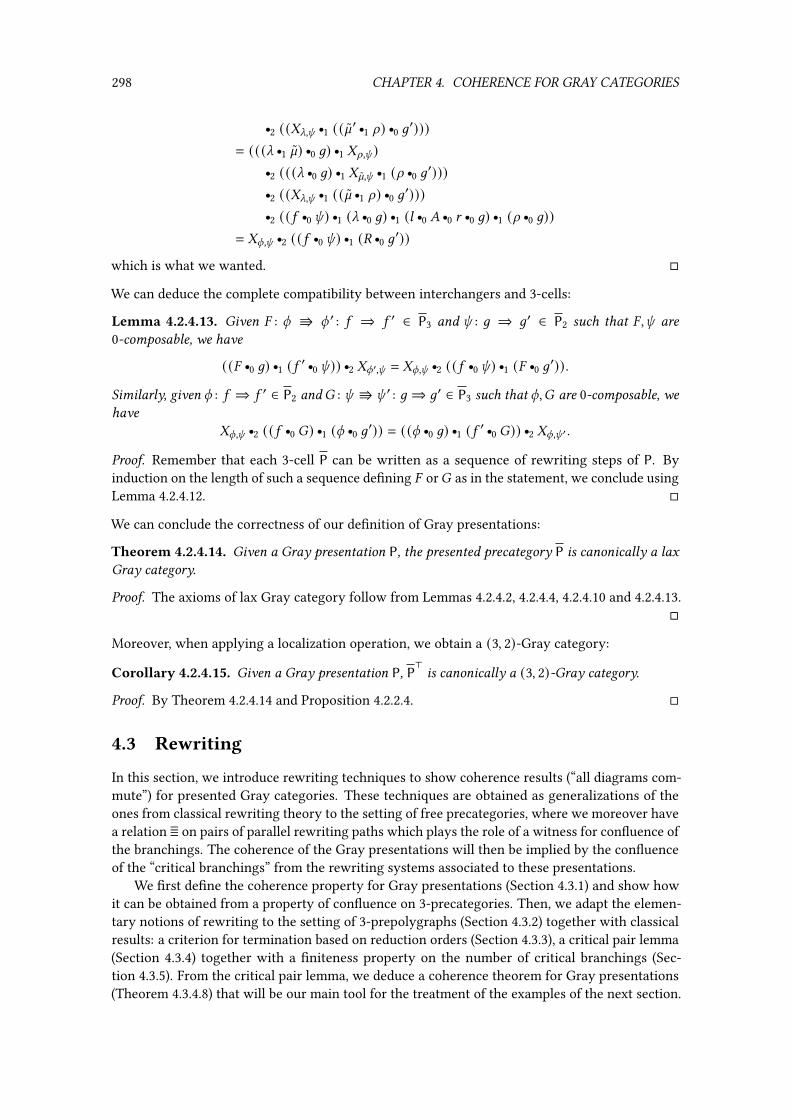
298 CHAPTER 4. COHERENCE FOR GRAY CATEGORIES

r2 ((-_,k r1 (( ˜ ′ r1 d) r0 6′)))= (((_ r1 ˜) r0 6) r1 -d,k )r2 (((_ r0 6) r1 - ˜,k r1 (d r0 6′)))r2 ((-_,k r1 (( ˜ r1 d) r0 6′)))r2 ((5 r0 k ) r1 (_ r0 6) r1 (; r0 � r0 A r0 6) r1 (d r0 6))= -q,k r2 ((5 r0 k ) r1 (' r0 6′))

which is what we wanted. �

We can deduce the complete compatibility between interchangers and 3-cells:

Lemma 4.2.4.13. Given � : q V q ′ : 5 ⇒ 5 ′ ∈ P3 and k : 6 ⇒ 6′ ∈ P2 such that �,k are0-composable, we have

((� r0 6) r1 (5 ′ r0 k )) r2 -q′,k = -q,k r2 ((5 r0 k ) r1 (� r0 6′)).Similarly, given q : 5 ⇒ 5 ′ ∈ P2 and� : k V k ′ : 6⇒ 6′ ∈ P3 such that q,� are 0-composable, wehave

-q,k r2 ((5 r0 �) r1 (q r0 6′)) = ((q r0 6) r1 (5 ′ r0 �)) r2 -q,k ′ .Proof. Remember that each 3-cell P can be written as a sequence of rewriting steps of P. Byinduction on the length of such a sequence de�ning � or� as in the statement, we conclude usingLemma 4.2.4.12. �

We can conclude the correctness of our de�nition of Gray presentations:

Theorem 4.2.4.14. Given a Gray presentation P, the presented precategory P is canonically a laxGray category.

Proof. The axioms of lax Gray category follow from Lemmas 4.2.4.2, 4.2.4.4, 4.2.4.10 and 4.2.4.13.�

Moreover, when applying a localization operation, we obtain a (3, 2)-Gray category:

Corollary 4.2.4.15. Given a Gray presentation P, P>is canonically a (3, 2)-Gray category.

Proof. By Theorem 4.2.4.14 and Proposition 4.2.2.4. �

4.3 Rewriting

In this section, we introduce rewriting techniques to show coherence results (“all diagrams com-mute”) for presented Gray categories. These techniques are obtained as generalizations of theones from classical rewriting theory to the setting of free precategories, where we moreover havea relation == on pairs of parallel rewriting paths which plays the role of a witness for con�uence ofthe branchings. The coherence of the Gray presentations will then be implied by the con�uenceof the “critical branchings” from the rewriting systems associated to these presentations.

We �rst de�ne the coherence property for Gray presentations (Section 4.3.1) and show howit can be obtained from a property of con�uence on 3-precategories. Then, we adapt the elemen-tary notions of rewriting to the setting of 3-prepolygraphs (Section 4.3.2) together with classicalresults: a criterion for termination based on reduction orders (Section 4.3.3), a critical pair lemma(Section 4.3.4) together with a �niteness property on the number of critical branchings (Sec-tion 4.3.5). From the critical pair lemma, we deduce a coherence theorem for Gray presentations(Theorem 4.3.4.8) that will be our main tool for the treatment of the examples of the next section.

4.3. REWRITING 299

4.3.1 Coherence in Gray categories

Recall that the aim of this chapter is to provide tools to study the coherence of presented Graycategories. Below, we de�ne this notion and give a �rst criterion to obtain the coherence of(3, 2)-precategories obtained by the localization functor.

4.3.1.1 — De�nition. A 3-precategory � is coherent when, for every pair of parallel 3-cells

�1, �2 : q V k ∈ �3

we have �1 = �2. A Gray presentation P is then coherent when the underlying (3, 2)-preca-tegory of the (3, 2)-Gray category P

> is coherent (remember that P is a lax Gray category byTheorem 4.2.4.14, which implies that P> is a (3, 2)-Gray category by Proposition 4.2.2.4). Graypresentations P with no other 4-generators than the independence generators and the interchangenaturality generators are usually not coherent. For example, in the Gray presentation P of pseu-domonoids given in Example 4.2.3.3, we do not expect the following parallel 3-cells

to be equal in P>. For coherence, we need to add “tiles” in P4 to �ll the “holes” created by parallel

3-cells as the ones above. A trivial way to do this is to add a 4-generator ' : �1 �2 for every pairof parallel 3-cells �1 and �2 of P∗. However, this method gives quite big presentations, whereaswe aim at small ones, so that the number of axioms to verify in concrete instances is as little aspossible. We expose a better method in Section 4.3.4, in the form of Theorem 4.3.4.8: we will seethat it is enough to add a tile of the form

q

q1 == q2

k

(1 (1

�1 �2

for every critical branching ((1, (2) of P for which we chose rewriting paths �1, �2 that make thebranching ((1, (2) joinable (de�nitions are introduced below).

4.3.1.2 — Coherence from con�uence. We now show how the coherence property can beobtained starting from 3-precategory whose 3-cells satisfy a property of con�uence, motivatingthe adaptation of rewriting theory to 3-prepolygraphs in order to study the coherence of Graypresentations. In fact, we can already prove an analogue of the Church-Rosser property comingfrom rewriting theory in the context of con�uent categories.

A 3-precategory � is con�uent when, for 2-cells q, q1, q2 ∈ �2 and 3-cells

�1 : q V q1 and �2 : q V q2

of � , there exist a 2-cellk ∈ �2 and 3-cells

�1 : q1 V k ∈ �3 and �2 : q2 V k ∈ �3

300 CHAPTER 4. COHERENCE FOR GRAY CATEGORIES

of � such that �1 r2 �1 = �2 r2 �2. The 3-cells of a (3, 2)-precategory associated to a con�uent3-precategory admits a simple form, as in:

Proposition 4.3.1.3. Given a con�uent 3-precategory � , all � : q V q ′ ∈ �>3 can be writ-ten � = � r2 �−1 for somek ∈ �2, � : q V k ∈ �3 and � : q ′ V k ∈ �3.

The above property says that con�uent categories satisfy a “Church-Rosser property” ([BN99,De�nition 2.1.3], for example), and is analogous to the classical result stating that con�uentrewriting systems are Church-Rosser ([BN99, Theorem 2.1.5], for example).

Proof. By the de�nition of �>, all 3-cell � : q V q ′ ∈ �>3 can be written

� = �−11

r2 �1 r2 · · · r2 �−1:

r2 �:for some : ∈ N and 3-cells�8 : j8 V q8−1 and�8 : j8 V q8 of� for 8 ∈ N∗

:withq0 = q andq: = q ′,

as inj1 · · · j:

q0 q1 · · · q:−1 q:

�1 �1 �2 �:−1 �: �: .

We prove the property by induction on : . If : = 0, then � is an identity and the result follows.Otherwise, since� is con�uent, there existsk: ∈ �2,� ′

:: q:−1 V k: ∈ �3 and � ′

:: q: V k: ∈ �3

withj:

q:−1 = q:

k:

�: �:

�′:

� ′:

.

By induction, the morphism

�−11

r2 �1 r2 · · · r2 �−1:−2

r2 �:−2 r2 �−1:−1

r2 (�:−1 r2 � ′: )can be written � r2 �−1 for some 2-cellk and 3-cells � : q0 V k and � : k: V k of � . Since

�: r2 � ′: = �: r2 � ′: ,

we have �−1:

r2 �: = � ′:r2 � ′−1

:. Hence,

� = � r2 �−1 r2 � ′−1:

= � r2 (� ′: r2 � )−1

which is of the wanted form. �

Starting from a con�uent 3-precategory, we have the following simple criterion to deduce thecoherence of the associated (3, 2)-precategory:

Proposition 4.3.1.4. Let � be a con�uent 3-precategory which moreover satis�es that, for everypair of parallel 3-cells �1, �2 : q V q ′ of � , we have �1 = �2 in the localization �>. Then, �>

is coherent. In particular, if � is a con�uent 3-precategory satisfying that, for all pair of parallel3-cells �1, �2 : q V q ′ of � , there exists� : q ′ V q ′′ ∈ �3 such that �1 r2 � = �2 r2 � in �3, then �>

is coherent.

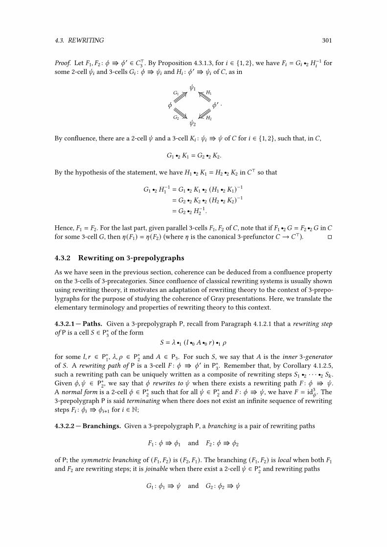
4.3. REWRITING 301

Proof. Let �1, �2 : q V q ′ ∈ �>3 . By Proposition 4.3.1.3, for 8 ∈ {1, 2}, we have �8 = �8 r2 �−18 for

some 2-cellk8 and 3-cells �8 : q V k8 and �8 : q ′ V k8 of � , as in

k1

q q ′

k2

�1

�2

�1

�2

.

By con�uence, there are a 2-cellk and a 3-cell 8 : k8 V k of � for 8 ∈ {1, 2}, such that, in � ,

�1 r2 1 = �2 r2 2.

By the hypothesis of the statement, we have �1 r2 1 = �2 r2 2 in �> so that

�1 r2 �−11 = �1 r2 1 r2 (�1 r2 1)−1

= �2 r2 2 r2 (�2 r2 2)−1

= �2 r2 �−12 .

Hence, �1 = �2. For the last part, given parallel 3-cells �1, �2 of� , note that if �1 r2� = �2 r2� in�for some 3-cell � , then [ (�1) = [ (�2) (where [ is the canonical 3-prefunctor � → �>). �

4.3.2 Rewriting on 3-prepolygraphs

As we have seen in the previous section, coherence can be deduced from a con�uence propertyon the 3-cells of 3-precategories. Since con�uence of classical rewriting systems is usually shownusing rewriting theory, it motivates an adaptation of rewriting theory to the context of 3-prepo-lygraphs for the purpose of studying the coherence of Gray presentations. Here, we translate theelementary terminology and properties of rewriting theory to this context.

4.3.2.1 — Paths. Given a 3-prepolygraph P, recall from Paragraph 4.1.2.1 that a rewriting stepof P is a cell ( ∈ P∗3 of the form

( = _ r1 (; r0 � r0 A ) r1 dfor some ;, A ∈ P∗1, _, d ∈ P∗2 and � ∈ P3. For such ( , we say that � is the inner 3-generatorof ( . A rewriting path of P is a 3-cell � : q V q ′ in P∗3. Remember that, by Corollary 4.1.2.5,such a rewriting path can be uniquely written as a composite of rewriting steps (1 r2 · · · r2 (: .Given q,k ∈ P∗2, we say that q rewrites to k when there exists a rewriting path � : q V k .A normal form is a 2-cell q ∈ P∗2 such that for all k ∈ P∗2 and � : q V k , we have � = id3

q. The

3-prepolygraph P is said terminating when there does not exist an in�nite sequence of rewritingsteps �8 : q8 V q8+1 for 8 ∈ N;

4.3.2.2 — Branchings. Given a 3-prepolygraph P, a branching is a pair of rewriting paths

�1 : q V q1 and �2 : q V q2

of P; the symmetric branching of (�1, �2) is (�2, �1). The branching (�1, �2) is local when both �1and �2 are rewriting steps; it is joinable when there exist a 2-cellk ∈ P∗2 and rewriting paths

�1 : q1 V k and �2 : q2 V k

302 CHAPTER 4. COHERENCE FOR GRAY CATEGORIES

of P; given a congruence == on P∗, if we moreover have that �1 r2 �1 == �2 r2 �2, as in

q

q1 == q2

k

�1 �2

�1 �2

we say that the branching is con�uent for ==.

4.3.2.3 — Rewriting systems. A rewriting system (P,==) is the data of a 3-prepolygraph P to-gether with a congruence == on P∗. (P,==) is (locally) con�uent when every (local) branching iscon�uent for ==; it is convergent when it is locally con�uent and P is terminating.

Given a 4-prepolygraph P, the rewriting system associated to P is (P≤3,∼P) (recall the de�nitionof ∼P given in Section 4.1.3) where ∼P intuitively witnesses that the “space” between two parallel3-cells can be �lled with elementary tiles that are the elements of P4. In the following, most ofthe concrete rewriting systems that we study are of this form.

4.3.2.4 — Newman’s lemma. Our de�nition of rewriting system contrasts with the classicalde�nitions of abstract or term rewriting systems, in which all pairs of parallel paths are equal.Nevertheless, the analogues of several well-known properties of abstract rewriting systems canbe proved in our context. In particular, the classical proof by well-founded induction of Newman’slemma ([BN99, Lemma 2.7.2], for example), can be directly adapted in order to show that:

Theorem 4.3.2.5. A convergent rewriting system is con�uent.

Proof. Let (P,==) be a rewriting system which is convergent. LetV+ ⊆ P∗2×P∗2 be the partial ordersuch thatq V+ k if there exists a rewriting path � : q V k ∈ P∗3 with |� | > 0. Since the underlyingrewriting system is terminating,V+ is well-founded. Thus, we can prove the theorem by inductiononV+. So suppose given a branching �1 : q V q1 ∈ P∗3 and �2 : q V q2 ∈ P∗3. If |�1 | = 0 or |�2 | = 0,then the branching is con�uent. Otherwise, for 8 ∈ {1, 2}, �8 = (8 r2 � ′8 for some rewritingstep (8 : q V q ′8 and rewriting path � ′8 : q ′8 V q8 . Since the rewriting system is locally con�uent,there arek ∈ P∗2 and rewriting paths �8 : q ′8 V k for 8 ∈ {1, 2} such that (1 r2 �1 == (2 r2 �2. Sincethe rewriting system is terminating and == is stable by composition, by composing the�8 ’s with apath� : k V k ′ wherek ′ is a normal form, we can suppose thatk is a normal form. By inductionon q ′1 and q ′2, there are rewriting paths �8 : q8 V k ′8 and � ′′8 : k V k ′8 such that � ′8 r2 �8 == �8 r2 � ′′8for 8 ∈ {1, 2}. Sincek is in normal form, � ′′8 = id3

kand we have �8 : q8 V k for 8 ∈ {1, 2} as in

q

q ′1 q ′2

q1 k q2

==

(1 (2

� ′1 �1 �2 � ′2

�1 �2

== ==

.

Moreover,

�1 r2 �1 == (1 r2 (� ′1 r2 �1)== (1 r2 �1== (2 r2 �2== (2 r2 (� ′2 r2 �2)== �2 r2 �2. �

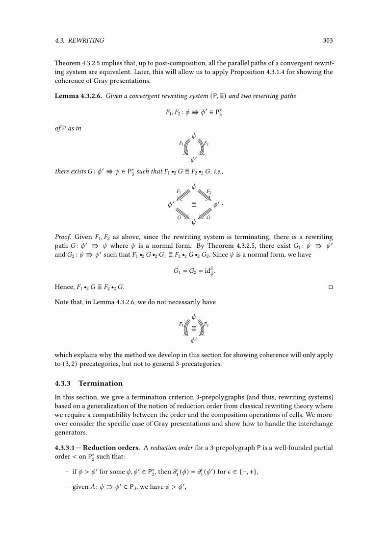
4.3. REWRITING 303

Theorem 4.3.2.5 implies that, up to post-composition, all the parallel paths of a convergent rewrit-ing system are equivalent. Later, this will allow us to apply Proposition 4.3.1.4 for showing thecoherence of Gray presentations.

Lemma 4.3.2.6. Given a convergent rewriting system (P,==) and two rewriting paths

�1, �2 : q V q ′ ∈ P∗3

of P as inq

q ′

�1 �2

there exists � : q ′ V k ∈ P∗3 such that �1 r2 � == �2 r2 � , i.e.,q

q ′ == q ′

k

�1 �2

� �

.

Proof. Given �1, �2 as above, since the rewriting system is terminating, there is a rewritingpath � : q ′ V k where k is a normal form. By Theorem 4.3.2.5, there exist �1 : k V k ′

and �2 : k V k ′ such that �1 r2 � r2 �1 == �2 r2 � r2 �2. Sincek is a normal form, we have

�1 = �2 = id3k

.

Hence, �1 r2 � == �2 r2 � . �

Note that, in Lemma 4.3.2.6, we do not necessarily have

q

q ′

�1 �2==

which explains why the method we develop in this section for showing coherence will only applyto (3, 2)-precategories, but not to general 3-precategories.

4.3.3 Termination

In this section, we give a termination criterion 3-prepolygraphs (and thus, rewriting systems)based on a generalization of the notion of reduction order from classical rewriting theory wherewe require a compatibility between the order and the composition operations of cells. We more-over consider the speci�c case of Gray presentations and show how to handle the interchangegenerators.

4.3.3.1 — Reduction orders. A reduction order for a 3-prepolygraph P is a well-founded partialorder < on P∗2 such that:

– if q > q ′ for some q, q ′ ∈ P∗2, then mn1 (q) = mn1 (q ′) for n ∈ {−, +},

– given � : q V q ′ ∈ P3, we have q > q ′,

304 CHAPTER 4. COHERENCE FOR GRAY CATEGORIES

– given ;, A ∈ P∗1 and q, q ′ ∈ P∗2 such that ;, q, A are 0-composable and q > q ′, we have

; r0 q r0 A > ; r0 q ′ r0 A ,– given 1-composable _, q, d ∈ P∗2, and q ′ ∈ P∗2 such that q > q ′, we have

_ r1 q r1 d > _ r1 q ′ r1 d .

One has then the following criterion to show the termination of a 3-prepolygraph:

Proposition 4.3.3.2. Given a 3-prepolygraph P, if there exists a reduction order for P, then P isterminating.

Proof. The de�nition of a reduction order implies that, given a rewriting step _ r1 (; r0 � r0 A ) r1 dwith ;, A ∈ P∗1, _, d ∈ P∗2 and � : q V q ′ ∈ P3 suitably composable, we have

_ r1 (; r0 q r0 A ) r1 d > _ r1 (; r0 q ′ r0 A ) r1 d.So, given a sequence of 2-composable rewriting steps (�8)8∈N: , where : ∈ N ∪ {l} and

�8 : q8 V q8+1 ∈ P∗3

for some q8 ∈ P∗2 for 8 ∈ N:+1, we have q 9 > q 9+1 for 9 ∈ N: . Since > is well-founded, it impliesthat : ∈ N. Hence, P is terminating. �

4.3.3.3 — The case of Gray presentations. In order to build a reduction order for a Gray presen-tation P, we have to build in particular a reduction order for the subset of P3 made of interchangegenerators. We introduce below a su�cient criterion for the existence of such a reduction order.The idea is to consider the lengths of the 1-cells of the whiskers in the decompositions of 2-cellsand show that they are decreasing in some way when an interchange generator is applied.

Let N<l be the set of �nite sequences of elements of N. We order N<l by <l where

(01, . . . , 0: ) <l (11, . . . , 1; )

when : = ; and there exists 8 ∈ N∗:

such that 0 9 = 1 9 for 9 ∈ N∗8−1 and 08 < 18 . Note that <l is well-founded. Given a 2-prepolygraph P, there is a function Int : P∗2 → N<l such that, given q ∈ P∗2,decomposed uniquely (using Corollary 4.1.2.5) as

q = (;1 r0 U1 r0 A1) r1 · · · r1 (;: r0 U: r0 A: )for some : ∈ N, ;8 , A8 ∈ P∗1 and U8 ∈ P2 for 8 ∈ N∗

:, Int(q) is de�ned by

Int(q) = ( |;: |, |;:−1 |, . . . , |;1 |).

Then, Int induces a partial order <int on P∗2 by putting q <int k when mn1 (q) = mn1 (k ) for n ∈ {−, +}and Int(q) <l Int(k ) for q,k ∈ P∗2.

Given a Gray presentation P, we say that P is positive when |m+1 (U) | > 0 for all U ∈ P2. Underpositiveness, the order <int can be considered as a reduction order for the subset of 3-generatorsof a Gray presentation made of interchangers:

Proposition 4.3.3.4. Let P be a positive Gray presentation. The partial order <int has the followingproperties:

4.3. REWRITING 305

(i) for every U, V ∈ P2 and 5 ∈ P∗1 such that U, 5 , V are 0-composable,

m−2 (-U,5 ,V ) >int m+2 (-U,5 ,V ),

(ii) for q, q ′ ∈ P∗2 and ;, A ∈ P∗1 such that ;, q, A are 0-composable, if q >int q′, then

; r0 q r0 A >int ; r0 q ′ r0 A ,(iii) for q, q ′, _, d ∈ P∗2 such that _, q, d are 1-composable, if q >int q

′, then

_ r1 q r1 d >int _ r1 q ′ r1 d .Proof. Given U, V ∈ P2 and 5 ∈ P∗1 with U, 5 , V are 0-composable, recall that -U,5 ,V is such that

-U,5 ,V : (U r0 5 r0 m−1 (V)) r1 (m+1 (U) r0 5 r0 V) V (m−1 (U) r0 5 r0 V) r1 (U r0 5 r0 m+1 (V)).Thus, we have

Int(m−2 (- )) = ( |m+1 (U) | + |5 |, 0) and Int(m+2 (- )) = (0, |m−1 (U) | + |5 |) .

Since P is positive, we have |m+1 (U) | > 0 so that Int(m−2 (- )) >int Int(m+2 (- )). Now, (ii) and (iii) canreadily be obtained by considering the whisker representations of q and q ′ and observing theaction of ; r0 − r0 A and _ r1 − r1 d on these representations and the de�nition of Int. �

The positiveness condition is required to prevent 2-cells with “�oating components”, since Graypresentations with such 2-cells might not terminate. For example, given a Gray presentation Pwhere P0 and P1 have one element and P2 has two 2-generators and , there are 2-cells of P∗with “�oating bubbles” which induce in�nite reduction sequence with interchange generators asthe following one:

V V V V V · · ·

4.3.4 Critical branchings

In term rewriting systems, a classical result called the “critical pair lemma” states that local con�u-ence is a consequence of the con�uence of a subset of local branchings, called critical branchings.The latter can be described as pairs of rewrite rules that are minimally overlapping (see [BN99,Section 6.2] for details). Here, we show a similar result for rewriting on Gray presentations. Forthis purpose, we �rst give a de�nition of critical branchings similar to the one of term rewrit-ing systems, i.e., as minimally overlapping local branchings, where we moreover �lter out somebranchings that involve interchange generators and that are readily con�uent by our de�nitionof Gray presentation. We then use this adapted critical pair lemma to prove coherence results forGray presentations.

4.3.4.1 — Classi�cation of branchings. Let P be a 3-prepolygraph. Given a local branching

((1 : q V q1, (2 : q V q2)

of P, we say that the branching ((1, (2) is

– trivial when (1 = (2,

306 CHAPTER 4. COHERENCE FOR GRAY CATEGORIES

– minimal when for all other local branching (( ′1, ( ′2) such that

(8 = _ r1 (; r0 ( ′8 r0 A ) r1 dfor 8 ∈ {1, 2} for some 1-cells ;, A and 2-cells _, d , we have that ;, A , _, d are all identities,

– independent when

(1 = ((;1 r0 �1 r0 A1) r1 j r1 (;2 r0 q2 r0 A2)) (2 = ((;1 r0 q1 r0 A1) r1 j r1 (;2 r0 �2 r0 A2))

for some ;8 , A8 ∈ P∗1 and �8 : q8 V q ′8 ∈ P3 for 8 ∈ {1, 2} and j ∈ P∗2.

If moreover P = Q≤3 where Q is a Gray presentation, we say that the branching ((1, (2) is

– natural when either(1 = (� r0 6 r0 ℎ) r1 (5 ′ r0 6 r0 V)

for some � : q V q ′ : 5 ⇒ 5 ′ ∈ P3, 6 ∈ P∗1 and V : ℎ ⇒ ℎ′ ∈ P2, and

(2 = [XD,n ]q,6 q0V with D = l1 . . . l |q |−1

or(1 = (U r0 6′ r0 ℎ) r1 (5 ′ r0 6′ r0 �)

for some U : 5 ⇒ 5 ′ ∈ P2, 6′ ∈ P∗1 and � : k V k ′ : ℎ ⇒ ℎ′ ∈ P3, and

(2 = [Xn,E]U,6′ q0k with E = r2 . . . r |k | ,

– critical when it is minimal, and both its symmetrical branching and it are neither trivialnor independent nor natural.

4.3.4.2 — Critical pair lemma. Let Q be a Gray presentation and write (P,==) for the rewritingsystem (Q≤3,∼Q). Our next goal is to show an adapted version of the classical critical pair lemmato our context. We start by two technical lemmas:

Lemma 4.3.4.3. For all local branching ((1, (2) of P, there is a minimal branching (( ′1, ( ′2) and1-cells ;, A ∈ P∗1 and 2-cells _, d ∈ P∗2 such that (8 = _ r1 (; r0 ( ′8 r0 A ) r1 d for 8 ∈ {1, 2}.

Proof. We show this by induction on # ((1) where # ((1) = |m−2 ((1) | + |m−1 ((1) |. Suppose that theproperty is true for all local branchings (( ′1, ( ′2) with # (( ′1) < # ((1). If ((1, (2) is not minimal,then there are rewriting steps ( ′1, (

′2 ∈ P∗3, ;, A ∈ P∗1 and _, d ∈ P∗2 such that (8 = _ r1 (; r0 ( ′8 r0 A ) r1 d

for 8 ∈ {1, 2}, such that ;, A , _, d are not all identities. Since

|m−1 ((1) | = |; | + |m−1 (( ′1) | + |A | and |m−2 ((1) | = |_ | + |m−2 (( ′1) | + |d |,

we have # (( ′1) < # ((1) so there is a minimal branching (( ′′1 , ( ′′2 ) and ; ′, A ′ ∈ P∗1, _′, d ′ ∈ P∗2 suchthat ( ′8 = _

′ r1 (; ′ r0( ′′8 r0A ′) r1 d ′ for 8 ∈ {1, 2}. By composing with _, d, ;, A , we obtain the conclusionof the lemma. �

Lemma 4.3.4.4. A local branching of P which is either trivial or independent or natural is con�uent.

Proof. A trivial branching is, of course, con�uent. Independent and natural branching are con�u-ent thanks respectively to the independence generators and interchange naturality generators ofa Gray presentation. �

4.3. REWRITING 307

The critical pair lemma adapted to our context is then:

Theorem 4.3.4.5 (Adapted critical pair lemma). The rewriting system (P,==) is locally con�uent ifand only if every critical branching is con�uent.

Proof. The �rst implication is trivial. For the converse, note that, by Lemma 4.3.4.3, in orderto check that all local branchings are con�uent, it is enough to check that all minimal localbranchings are con�uent. Among them, by Lemma 4.3.4.4, it is enough to check the con�uenceof the critical branchings. �

4.3.4.6 — Coherence results. We now state the main result of this section, namely a coherencetheorem for Gray presentations based on the analysis of the critical branchings:

Theorem 4.3.4.7 (Coherence). Let Q be a Gray presentation and (P,==) = (Q≤3,∼Q) be the asso-ciated rewriting system. If P is terminating and all the critical branchings of (P,==) are con�uent,then Q is a coherent Gray presentation.

Proof. By Theorem 4.3.4.5, the rewriting system (P,==) is locally con�uent, and by Theorem 4.3.2.5it is con�uent. Since Q = P∗/==, it implies that Q is a con�uent 3-precategory. To conclude, it issu�cient to show that the criterion in the last part of Proposition 4.3.1.4 is satis�ed. But the latteris a consequence of Lemma 4.3.2.6. �

Note that Theorem 4.3.4.7 requires the rewriting system (P,==) to be con�uent. If it is not thecase, one can still try to apply an analogue of the Knuth-Bendix completion algorithm ([BN99,Section 7], for example) and add 3-generators together with 4-generators to obtain a con�uentGray presentation, and then apply Theorem 4.3.4.7.

Our coherence theorem implies a coherence criterion similar to the ones shown by Squier etal. [SOK94, Theorem 5.2] and Guiraud et al. [GM09, Proposition 4.3.4], which states that addinga tile for each critical branching is enough to ensure coherence:

Theorem 4.3.4.8. LetQ be a Gray presentation and (P,==) = (Q≤3,∼Q) be the associated rewritingsystem. Suppose that, for every critical branching ((1 : q V q1, (2 : q V q2) of (P,==), there existcells k ∈ P∗2 and �8 : q8 V k ∈ P∗3 for 8 ∈ {1, 2}, and a 4-generator � : (1 r2 �1 (2 r2 �2 ∈ Q4.Then, Q is a coherent Gray presentation.

Proof. The de�nition of Q4 ensures that all the critical branchings are con�uent, so that Theo-rem 4.3.4.7 applies. �

Remark 4.3.4.9. In fact, for the conclusion of Theorem 4.3.4.8 to hold, for every critical branch-ing ((1, (2) of (P,==), it is enough to have a 4-generator� as in the statement for either ((1, (2) orthe symmetrical critical branching ((2, (1), so that a stronger statement holds.

4.3.5 Finiteness of critical branchings

In this section, we prove that Gray presentations, under some reasonable conditions, have a �nitenumber of critical branchings (Theorem 4.3.5.8). This property contrasts with the case of strictcategories, where �nite presentations can have an in�nite number of critical branchings [Laf03;GM09]. Our proof is moreover constructive, so that one can derive an algorithm to compute thecritical branchings of such Gray presentations.

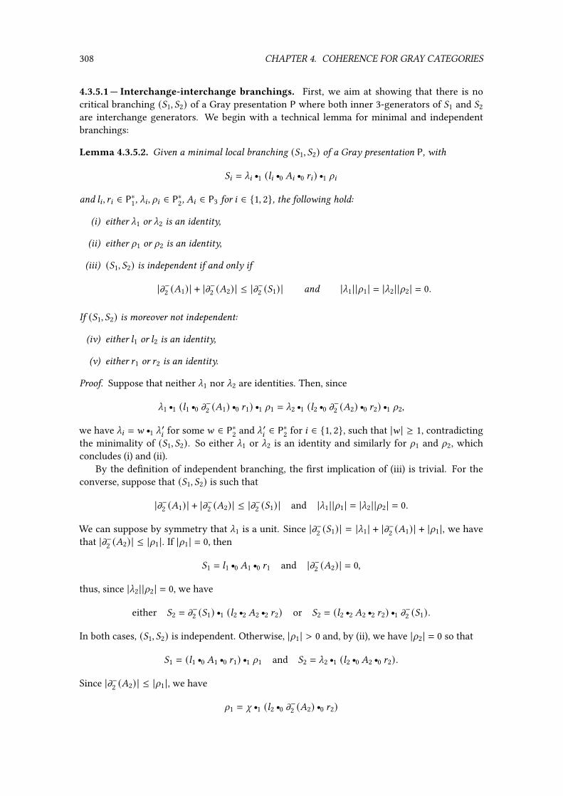
308 CHAPTER 4. COHERENCE FOR GRAY CATEGORIES

4.3.5.1 — Interchange-interchange branchings. First, we aim at showing that there is nocritical branching ((1, (2) of a Gray presentation P where both inner 3-generators of (1 and (2are interchange generators. We begin with a technical lemma for minimal and independentbranchings:

Lemma 4.3.5.2. Given a minimal local branching ((1, (2) of a Gray presentation P, with

(8 = _8 r1 (;8 r0 �8 r0 A8) r1 d8and ;8 , A8 ∈ P∗1, _8 , d8 ∈ P∗2, �8 ∈ P3 for 8 ∈ {1, 2}, the following hold:

(i) either _1 or _2 is an identity,

(ii) either d1 or d2 is an identity,

(iii) ((1, (2) is independent if and only if

|m−2 (�1) | + |m−2 (�2) | ≤ |m−2 ((1) | and |_1 | |d1 | = |_2 | |d2 | = 0.

If ((1, (2) is moreover not independent:

(iv) either ;1 or ;2 is an identity,

(v) either A1 or A2 is an identity.

Proof. Suppose that neither _1 nor _2 are identities. Then, since

_1 r1 (;1 r0 m−2 (�1) r0 A1) r1 d1 = _2 r1 (;2 r0 m−2 (�2) r0 A2) r1 d2,

we have _8 = F r1 _′8 for someF ∈ P∗2 and _′8 ∈ P∗2 for 8 ∈ {1, 2}, such that |F | ≥ 1, contradictingthe minimality of ((1, (2). So either _1 or _2 is an identity and similarly for d1 and d2, whichconcludes (i) and (ii).

By the de�nition of independent branching, the �rst implication of (iii) is trivial. For theconverse, suppose that ((1, (2) is such that

|m−2 (�1) | + |m−2 (�2) | ≤ |m−2 ((1) | and |_1 | |d1 | = |_2 | |d2 | = 0.

We can suppose by symmetry that _1 is a unit. Since |m−2 ((1) | = |_1 | + |m−2 (�1) | + |d1 |, we havethat |m−2 (�2) | ≤ |d1 |. If |d1 | = 0, then

(1 = ;1 r0 �1 r0 A1 and |m−2 (�2) | = 0,

thus, since |_2 | |d2 | = 0, we have

either (2 = m−2 ((1) r1 (;2 r2 �2 r2 A2) or (2 = (;2 r2 �2 r2 A2) r1 m−2 ((1) .

In both cases, ((1, (2) is independent. Otherwise, |d1 | > 0 and, by (ii), we have |d2 | = 0 so that

(1 = (;1 r0 �1 r0 A1) r1 d1 and (2 = _2 r1 (;2 r0 �2 r0 A2) .

Since |m−2 (�2) | ≤ |d1 |, we have

d1 = j r1 (;2 r0 m−2 (�2) r0 A2)

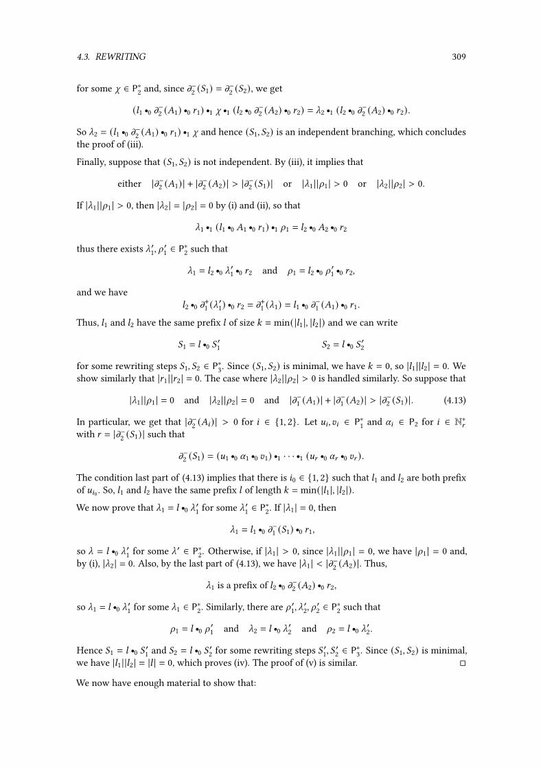
4.3. REWRITING 309

for some j ∈ P∗2 and, since m−2 ((1) = m−2 ((2), we get

(;1 r0 m−2 (�1) r0 A1) r1 j r1 (;2 r0 m−2 (�2) r0 A2) = _2 r1 (;2 r0 m−2 (�2) r0 A2) .

So _2 = (;1 r0 m−2 (�1) r0 A1) r1 j and hence ((1, (2) is an independent branching, which concludesthe proof of (iii).

Finally, suppose that ((1, (2) is not independent. By (iii), it implies that

either |m−2 (�1) | + |m−2 (�2) | > |m−2 ((1) | or |_1 | |d1 | > 0 or |_2 | |d2 | > 0.

If |_1 | |d1 | > 0, then |_2 | = |d2 | = 0 by (i) and (ii), so that

_1 r1 (;1 r0 �1 r0 A1) r1 d1 = ;2 r0 �2 r0 A2

thus there exists _′1, d′1 ∈ P∗2 such that

_1 = ;2 r0 _′1 r0 A2 and d1 = ;2 r0 d ′1 r0 A2,

and we have;2 r0 m+1 (_′1) r0 A2 = m

+1 (_1) = ;1 r0 m−1 (�1) r0 A1.

Thus, ;1 and ;2 have the same pre�x ; of size : = min( |;1 |, |;2 |) and we can write

(1 = ; r0 ( ′1 (2 = ; r0 ( ′2for some rewriting steps (1, (2 ∈ P∗3. Since ((1, (2) is minimal, we have : = 0, so |;1 | |;2 | = 0. Weshow similarly that |A1 | |A2 | = 0. The case where |_2 | |d2 | > 0 is handled similarly. So suppose that

|_1 | |d1 | = 0 and |_2 | |d2 | = 0 and |m−1 (�1) | + |m−1 (�2) | > |m−2 ((1) |. (4.13)

In particular, we get that |m−2 (�8) | > 0 for 8 ∈ {1, 2}. Let D8 , E8 ∈ P∗1 and U8 ∈ P2 for 8 ∈ N∗Awith A = |m−2 ((1) | such that

m−2 ((1) = (D1 r0 U1 r0 E1) r1 · · · r1 (DA r0 UA r0 EA ) .The condition last part of (4.13) implies that there is 80 ∈ {1, 2} such that ;1 and ;2 are both pre�xof D80 . So, ;1 and ;2 have the same pre�x ; of length : = min( |;1 |, |;2 |).We now prove that _1 = ; r0 _′1 for some _′1 ∈ P∗2. If |_1 | = 0, then

_1 = ;1 r0 m−1 ((1) r0 A1,

so _ = ; r0 _′1 for some _′ ∈ P∗2. Otherwise, if |_1 | > 0, since |_1 | |d1 | = 0, we have |d1 | = 0 and,by (i), |_2 | = 0. Also, by the last part of (4.13), we have |_1 | < |m−2 (�2) |. Thus,

_1 is a pre�x of ;2 r0 m−2 (�2) r0 A2,

so _1 = ; r0 _′1 for some _1 ∈ P∗2. Similarly, there are d ′1, _′2, d′2 ∈ P∗2 such that

d1 = ; r0 d ′1 and _2 = ; r0 _′2 and d2 = ; r0 _′2.Hence (1 = ; r0 ( ′1 and (2 = ; r0 ( ′2 for some rewriting steps ( ′1, (

′2 ∈ P∗3. Since ((1, (2) is minimal,

we have |;1 | |;2 | = |; | = 0, which proves (iv). The proof of (v) is similar. �

We now have enough material to show that:

310 CHAPTER 4. COHERENCE FOR GRAY CATEGORIES

Proposition 4.3.5.3. Given a Gray presentation P, there are no critical branching ((1, (2) of P suchthat both the inner 3-generators of (1 and (2 are interchange generators.

Proof. Let ((1, (2) be a local minimal branching such that, for 8 ∈ {1, 2},

(8 = _8 r1 (;8 r0 -U8 ,68 ,V8 r0 A8) r1 d8for some ;8 , A8 , 68 ∈ P∗1, _8 , d8 ∈ P∗2 and U8 , V8 ∈ P2, and let q be m−2 ((1). Since |m−2 (-U1,61,V1) | = 2, wehave |q | ≥ 2.

If |q | = 2, then |_8 | = |d8 | = 0 for 8 ∈ {1, 2}. Thus, since m−2 ((1) = m−2 ((2), we get

(;1 r0 U1 r0 61 r0 m−1 (V1) r0 A1) r1 (;1 r0 m+1 (U1) r0 61 r0 V1 r0 A1)= (;2 r0 U2 r0 62 r0 m−1 (V2) r0 A2) r1 (;2 r0 m+1 (U2) r0 62 r0 V2 r0 A2) .

By the unique decomposition property given by Theorem 4.1.2.4 and corollary 4.1.2.5, we obtain

;1 = ;2, A1 = A2, U1 = U2, V1 = V2 and 61 r0 m−1 (V1) r0 A1 = 62 r0 m−1 (V2) r0 A2.

So 61 r0 m−1 (V1) r0 A1 = 62 r0 m−1 (V1) r0 A1, which implies that 61 = 62. Hence, ((1, (2) is trivial.

If |q | = 3, then |_8 | + |d8 | = 1 for 8 ∈ {1, 2}, and, by Lemma 4.3.5.2,

either |d1 | = |_2 | = 1 or |_1 | = |d2 | = 1.

By symmetry, we can suppose that |d1 | = |_2 | = 1, which implies that |_1 | = |d2 | = 0. By uniquedecomposition of whiskers (Corollary 4.1.2.5), since m−2 ((1) = m−2 ((2), we have

;1 r0 U1 r0 61 r0 m−1 (V1) r0 A1 = _2

;1 r0 m+1 (U1) r0 61 r0 V1 r0 A1 = ;2 r0 U2 r0 62 r0 m−1 (V2) r0 A2

d1 = ;2 r0 m+1 (U2) r0 62 r0 V2 r0 A2

and the second line implies that ;1 r0 m+1 (U1) r061 = ;2, V1 = U2 and A1 = 62 r0 m−1 (V2) r0A2. Since ((1, (2)is minimal, we have |;1 | = |A2 | = 0. So

(1 = (-U1,61,V1r0 62 r0 m−1 (V2)) r1 (m+1 (-U1,61,V1) r0 62 r0 V2)

(2 = (U1 r0 61 r0 m−1 (V1) r0 62 r0 m−1 (V2)) r1 (m+1 (U1) r0 61 r0 -V1,62,V2)

thus ((1, (2) is a natural branching, hence not a critical one.

Finally, if |q | ≥ 4, then, since |_8 | + |d8 | = |q | − 2 ≥ 2 for 8 ∈ {1, 2}, by Lemma 4.3.5.2, we have that

either |_1 | = |d2 | = |q | − 2 or |d1 | = |_2 | = |q | − 2.

In either case,

|_1 | |d1 | = |_2 | |d2 | = 0 and |m−2 (-U1,61,V1) | + |m−2 (-U2,62,V2) | = 4 ≤ |q |

so, by Lemma 4.3.5.2(iii), ((1, (2) is independent, hence not critical. �

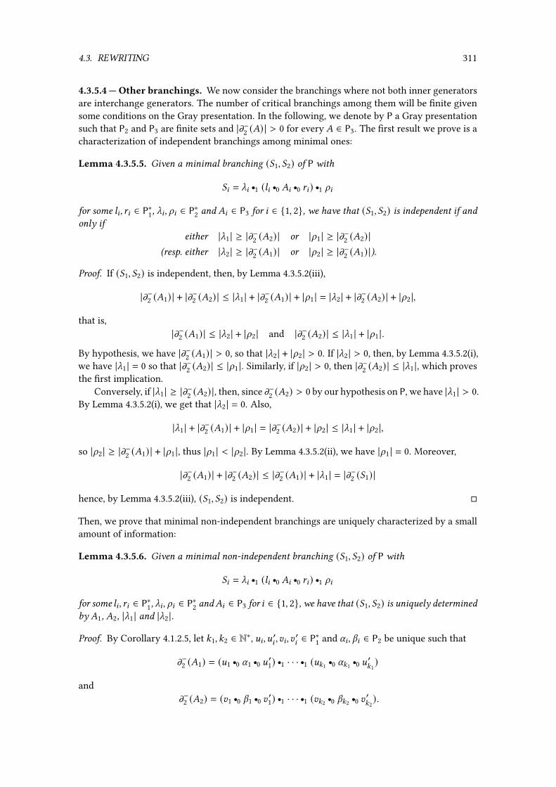
4.3. REWRITING 311

4.3.5.4 — Other branchings. We now consider the branchings where not both inner generatorsare interchange generators. The number of critical branchings among them will be �nite givensome conditions on the Gray presentation. In the following, we denote by P a Gray presentationsuch that P2 and P3 are �nite sets and |m−2 (�) | > 0 for every � ∈ P3. The �rst result we prove is acharacterization of independent branchings among minimal ones:

Lemma 4.3.5.5. Given a minimal branching ((1, (2) of P with

(8 = _8 r1 (;8 r0 �8 r0 A8) r1 d8for some ;8 , A8 ∈ P∗1, _8 , d8 ∈ P∗2 and �8 ∈ P3 for 8 ∈ {1, 2}, we have that ((1, (2) is independent if andonly if

either |_1 | ≥ |m−2 (�2) | or |d1 | ≥ |m−2 (�2) |(resp. either |_2 | ≥ |m−2 (�1) | or |d2 | ≥ |m−2 (�1) |).

Proof. If ((1, (2) is independent, then, by Lemma 4.3.5.2(iii),

|m−2 (�1) | + |m−2 (�2) | ≤ |_1 | + |m−2 (�1) | + |d1 | = |_2 | + |m−2 (�2) | + |d2 |,

that is,|m−2 (�1) | ≤ |_2 | + |d2 | and |m−2 (�2) | ≤ |_1 | + |d1 |.

By hypothesis, we have |m−2 (�1) | > 0, so that |_2 | + |d2 | > 0. If |_2 | > 0, then, by Lemma 4.3.5.2(i),we have |_1 | = 0 so that |m−2 (�2) | ≤ |d1 |. Similarly, if |d2 | > 0, then |m−2 (�2) | ≤ |_1 |, which provesthe �rst implication.

Conversely, if |_1 | ≥ |m−2 (�2) |, then, since m−2 (�2) > 0 by our hypothesis on P, we have |_1 | > 0.By Lemma 4.3.5.2(i), we get that |_2 | = 0. Also,

|_1 | + |m−2 (�1) | + |d1 | = |m−2 (�2) | + |d2 | ≤ |_1 | + |d2 |,

so |d2 | ≥ |m−2 (�1) | + |d1 |, thus |d1 | < |d2 |. By Lemma 4.3.5.2(ii), we have |d1 | = 0. Moreover,

|m−2 (�1) | + |m−2 (�2) | ≤ |m−2 (�1) | + |_1 | = |m−2 ((1) |

hence, by Lemma 4.3.5.2(iii), ((1, (2) is independent. �

Then, we prove that minimal non-independent branchings are uniquely characterized by a smallamount of information:

Lemma 4.3.5.6. Given a minimal non-independent branching ((1, (2) of P with

(8 = _8 r1 (;8 r0 �8 r0 A8) r1 d8for some ;8 , A8 ∈ P∗1, _8 , d8 ∈ P∗2 and�8 ∈ P3 for 8 ∈ {1, 2}, we have that ((1, (2) is uniquely determinedby �1, �2, |_1 | and |_2 |.

Proof. By Corollary 4.1.2.5, let :1, :2 ∈ N∗, D8 , D ′8 , E8 , E ′8 ∈ P∗1 and U8 , V8 ∈ P2 be unique such that

m−2 (�1) = (D1 r0 U1 r0 D ′1) r1 · · · r1 (D:1r0 U:1

r0 D ′:1)

andm−2 (�2) = (E1 r0 V1 r0 E ′1) r1 · · · r1 (E:2

r0 V:2r0 E ′:2).

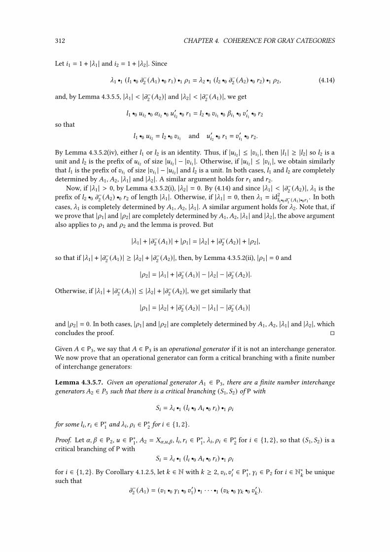
312 CHAPTER 4. COHERENCE FOR GRAY CATEGORIES

Let 81 = 1 + |_1 | and 82 = 1 + |_2 |. Since

_1 r1 (;1 r0 m−2 (�1) r0 A1) r1 d1 = _2 r1 (;2 r0 m−2 (�2) r0 A2) r1 d2, (4.14)

and, by Lemma 4.3.5.5, |_1 | < |m−2 (�2) | and |_2 | < |m−2 (�1) |, we get

;1 r0 D82 r0 U82 r0 D ′82 r0 A1 = ;2 r0 E81 r0 V81 r0 E ′81 r0 A2

so that;1 r0 D82 = ;2 r0 E81 and D ′82

r0 A1 = E′81

r0 A2.

By Lemma 4.3.5.2(iv), either ;1 or ;2 is an identity. Thus, if |D82 | ≤ |E81 |, then |;1 | ≥ |;2 | so ;2 is aunit and ;2 is the pre�x of D82 of size |D82 | − |E81 |. Otherwise, if |D82 | ≤ |E81 |, we obtain similarlythat ;1 is the pre�x of E81 of size |E81 | − |D82 | and ;2 is a unit. In both cases, ;1 and ;2 are completelydetermined by �1, �2, |_1 | and |_2 |. A similar argument holds for A1 and A2.

Now, if |_1 | > 0, by Lemma 4.3.5.2(i), |_2 | = 0. By (4.14) and since |_1 | < |m−2 (�2) |, _1 is thepre�x of ;2 r0 m−2 (�2) r0 A2 of length |_1 |. Otherwise, if |_1 | = 0, then _1 = id2

;1 q0m−1 (�1) q0A1. In both

cases, _1 is completely determined by �1, �2, |_1 |. A similar argument holds for _2. Note that, ifwe prove that |d1 | and |d2 | are completely determined by�1,�2, |_1 | and |_2 |, the above argumentalso applies to d1 and d2 and the lemma is proved. But

|_1 | + |m−2 (�1) | + |d1 | = |_2 | + |m−2 (�2) | + |d2 |,

so that if |_1 | + |m−2 (�1) | ≥ |_2 | + |m−2 (�2) |, then, by Lemma 4.3.5.2(ii), |d1 | = 0 and

|d2 | = |_1 | + |m−2 (�1) | − |_2 | − |m−2 (�2) |.

Otherwise, if |_1 | + |m−2 (�1) | ≤ |_2 | + |m−2 (�2) |, we get similarly that

|d1 | = |_2 | + |m−2 (�2) | − |_1 | − |m−2 (�1) |

and |d2 | = 0. In both cases, |d1 | and |d2 | are completely determined by�1,�2, |_1 | and |_2 |, whichconcludes the proof. �

Given � ∈ P3, we say that � ∈ P3 is an operational generator if it is not an interchange generator.We now prove that an operational generator can form a critical branching with a �nite numberof interchange generators:

Lemma 4.3.5.7. Given an operational generator �1 ∈ P3, there are a �nite number interchangegenerators �2 ∈ %3 such that there is a critical branching ((1, (2) of P with

(8 = _8 r1 (;8 r0 �8 r0 A8) r1 d8for some ;8 , A8 ∈ P∗1 and _8 , d8 ∈ P∗2 for 8 ∈ {1, 2}.

Proof. Let U, V ∈ P2, D ∈ P∗1, �2 = -U,D,V , ;8 , A8 ∈ P∗1, _8 , d8 ∈ P∗2 for 8 ∈ {1, 2}, so that ((1, (2) is acritical branching of P with

(8 = _8 r1 (;8 r0 �8 r0 A8) r1 d8for 8 ∈ {1, 2}. By Corollary 4.1.2.5, let : ∈ N with : ≥ 2, E8 , E ′8 ∈ P∗1, W8 ∈ P2 for 8 ∈ N∗

:be unique

such thatm−2 (�1) = (E1 r0 W1 r0 E ′1) r1 · · · r1 (E: r0 W: r0 E ′: ).

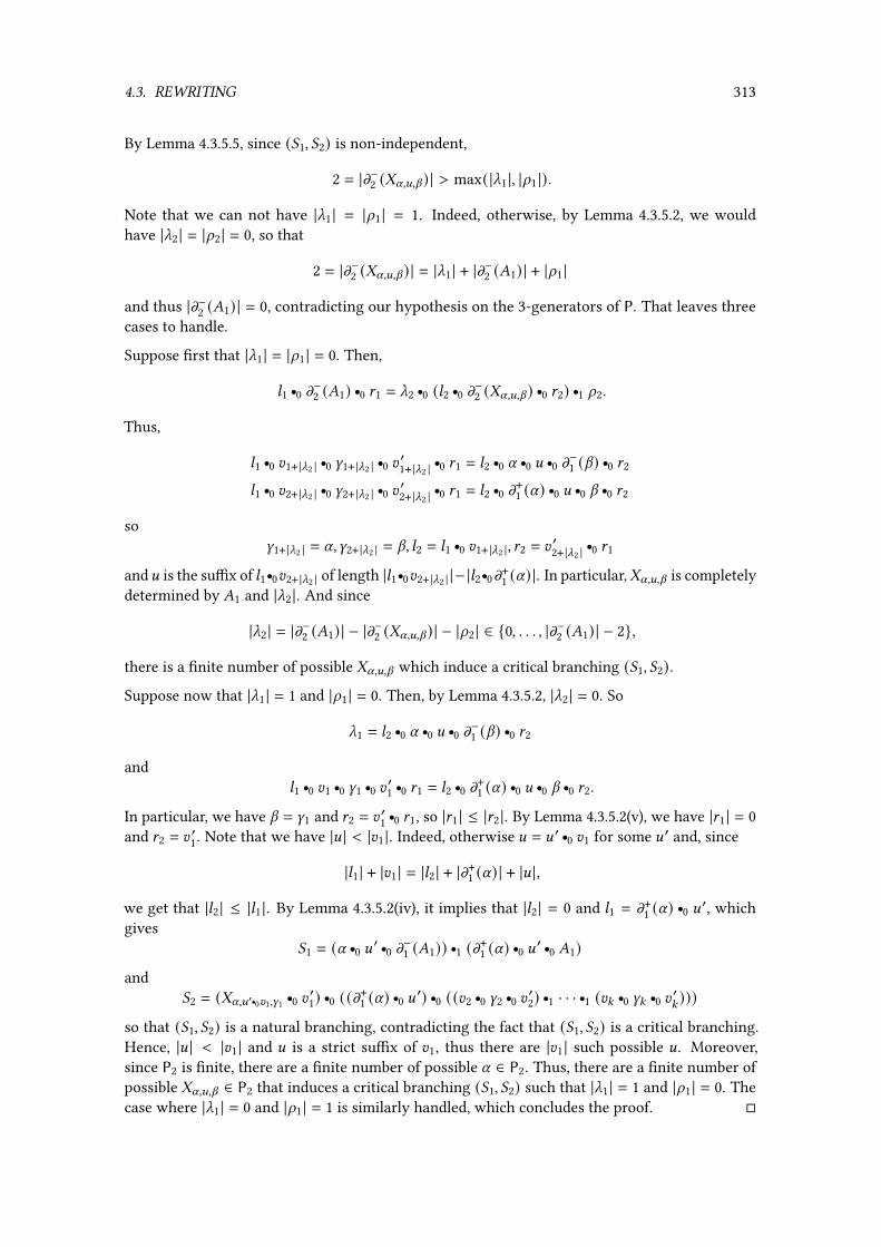
4.3. REWRITING 313

By Lemma 4.3.5.5, since ((1, (2) is non-independent,

2 = |m−2 (-U,D,V ) | > max( |_1 |, |d1 |).

Note that we can not have |_1 | = |d1 | = 1. Indeed, otherwise, by Lemma 4.3.5.2, we wouldhave |_2 | = |d2 | = 0, so that

2 = |m−2 (-U,D,V ) | = |_1 | + |m−2 (�1) | + |d1 |

and thus |m−2 (�1) | = 0, contradicting our hypothesis on the 3-generators of P. That leaves threecases to handle.

Suppose �rst that |_1 | = |d1 | = 0. Then,

;1 r0 m−2 (�1) r0 A1 = _2 r0 (;2 r0 m−2 (-U,D,V ) r0 A2) r1 d2.

Thus,

;1 r0 E1+|_2 | r0 W1+|_2 | r0 E ′1+|_2 |r0 A1 = ;2 r0 U r0 D r0 m−1 (V) r0 A2

;1 r0 E2+|_2 | r0 W2+|_2 | r0 E ′2+|_2 |r0 A1 = ;2 r0 m+1 (U) r0 D r0 V r0 A2

soW1+|_2 | = U,W2+|_2 | = V, ;2 = ;1 r0 E1+|_2 |, A2 = E

′2+|_2 |

r0 A1

andD is the su�x of ;1 r0E2+|_2 | of length |;1 r0E2+|_2 | |− |;2 r0 m+1 (U) |. In particular,-U,D,V is completelydetermined by �1 and |_2 |. And since

|_2 | = |m−2 (�1) | − |m−2 (-U,D,V ) | − |d2 | ∈ {0, . . . , |m−2 (�1) | − 2},

there is a �nite number of possible -U,D,V which induce a critical branching ((1, (2).

Suppose now that |_1 | = 1 and |d1 | = 0. Then, by Lemma 4.3.5.2, |_2 | = 0. So

_1 = ;2 r0 U r0 D r0 m−1 (V) r0 A2

and;1 r0 E1 r0 W1 r0 E ′1 r0 A1 = ;2 r0 m+1 (U) r0 D r0 V r0 A2.

In particular, we have V = W1 and A2 = E′1r0 A1, so |A1 | ≤ |A2 |. By Lemma 4.3.5.2(v), we have |A1 | = 0

and A2 = E′1. Note that we have |D | < |E1 |. Indeed, otherwise D = D ′ r0 E1 for some D ′ and, since

|;1 | + |E1 | = |;2 | + |m+1 (U) | + |D |,

we get that |;2 | ≤ |;1 |. By Lemma 4.3.5.2(iv), it implies that |;2 | = 0 and ;1 = m+1 (U) r0 D ′, whichgives

(1 = (U r0 D ′ r0 m−1 (�1)) r1 (m+1 (U) r0 D ′ r0 �1)

and(2 = (-U,D′ q0E1,W1

r0 E ′1) r0 ((m+1 (U) r0 D ′) r0 ((E2 r0 W2 r0 E ′2) r1 · · · r1 (E: r0 W: r0 E ′: )))so that ((1, (2) is a natural branching, contradicting the fact that ((1, (2) is a critical branching.Hence, |D | < |E1 | and D is a strict su�x of E1, thus there are |E1 | such possible D. Moreover,since P2 is �nite, there are a �nite number of possible U ∈ P2. Thus, there are a �nite number ofpossible -U,D,V ∈ P2 that induces a critical branching ((1, (2) such that |_1 | = 1 and |d1 | = 0. Thecase where |_1 | = 0 and |d1 | = 1 is similarly handled, which concludes the proof. �

314 CHAPTER 4. COHERENCE FOR GRAY CATEGORIES

With the above results, we can conclude the following �niteness property for critical branchingsof Gray presentations:

Theorem 4.3.5.8. Given a Gray presentation P where P2 and P3 are �nite and |m−2 (�) | > 0 forevery � ∈ P3, there is a �nite number of critical branchings of P.

Proof. Let (8 = _8 r1 (;8 r0 �8 r0 A8) r1 d8 with ;8 , A8 ∈ P∗1, _8 , d8 ∈ P∗2 and �8 ∈ P3 for 8 ∈ {1, 2}such that ((1, (2) is a critical branching of P. By Lemma 4.3.5.6, such a branching is uniquelydetermined by �1, �2, |_1 | and |_2 |. By Lemma 4.3.5.5,

|_1 | < |m−2 (�2) | and |_2 | < |m−2 (�1) |.

Hence, for a given pair (�1, �2), there are a �nite number of tuples (;1, ;2, A1, A2, _1, _2, d1, d2)such that ((1, (2) is a critical branching. Moreover, by Proposition 4.3.5.3, either �1 or �2 is anoperational generator. By symmetry, we can suppose that �1 is operational. Since P3 is �nite,there is a �nite number of such�1. Moreover, there are a �nite number of pairs (�1, �2) where�2is operational too. If �2 is an interchange generator, then, by Lemma 4.3.5.7, there are a �nitenumber of possible �2 for a given �1 such that ((1, (2) is a critical branching, which concludesthe �niteness analysis. �

Remark 4.3.5.9. The proof of Theorem 4.3.5.8 happens to be constructive, so that we can extractan algorithm to compute the critical branchings for such Gray presentations. An implementationof this algorithm was used to compute the critical branchings of the examples of the next section.

4.4 Applications

We now illustrate the techniques of the previous section and show the coherence of Gray pre-sentations related to several well-known algebraic structures. For each structure, we introduce aGray presentation and study the con�uence of the critical branchings of the associated rewritingsystem. Then, when the rewriting system is terminating, we can directly apply Theorem 4.3.4.8 todeduce the coherence of the presentation. This will be the case for pseudomonoids (Section 4.4.1),pseudoadjunctions (Section 4.4.2) and Frobenius pseudomonoids (Section 4.4.3) even though, inthe latter example, the termination of the rewriting system is assumed. We moreover study theexample of self-dualities, where the associated rewriting system is not terminating, for which weuse speci�c techniques in order to prove a weak coherence result.

4.4.1 Pseudomonoids

In Example 4.2.3.3, we introduced a Gray presentation P for the theory of pseudomonoids. Theset P4 of 4-generators contains only the required ones in a Gray presentation, so that we do notexpect P to be coherent. Below, we compute the critical branchings of the associated rewritingsystem and show that the latter is terminating. Thus, by Theorem 4.3.4.8, adding a 4-generatorcorresponding to each critical branching will turn the presentation into a coherent one. Ourmethod thus allows recovering a coherent de�nition for pseudomonoids in Gray categories, eventhough in a less compact form than the existing ones [SD97; Mar97; Lac00].

4.4.1.1 — Critical branchings. The critical branching of P can be computed by following theproof of Theorem 4.3.5.8, which is constructive. We obtain, up to symmetrical branchings, �ve

4.4. APPLICATIONS 315

critical branchings:

.

We observe that each of these branchings is joinable, and we de�ne �ve formal new 4-generatorsthat �ll the holes:

'1 '2 '3

'4 '5 .

We then de�ne PMon as the Gray presentation obtained from P de�ned in Example 4.2.3.3 byadding the 4-generators '1, . . . , '5 to P4.

4.4.1.2 — Termination. In order to use our coherence criterion on PMon, we need to show thetermination of the associated rewriting system. For this purpose, we use the tools of Section 4.3and build a reduction order. We �rst de�ne an order that handles the termination of the L,R,Agenerators, and then combine it with the order from Paragraph 4.3.3.3 to obtain a reduction order.For the �rst task, we use a similar technique than the one used in [Laf92]. Given = ∈ N, wewrite <∃ for the partial order on N= such that, given G,~ ∈ N= , G <∃ ~ when G8 ≤ ~8 for all 8 ∈ N∗=and there exists 9 ∈ N∗= such that G 9 < ~ 9 . Let N-Fun be the 2-precategory

– which has only one 0-cell, denoted ∗,

– whose 1-cells ∗ → ∗ are the natural numbers = ∈ N,

– whose 2-cells< ⇒ = for<,= ∈ N are the strictly monotone functions

q : (N<, <∃) → (N=, <∃),

and whose structural operations are such that

316 CHAPTER 4. COHERENCE FOR GRAY CATEGORIES

– id1∗ = 0,

– composition of 1-cells is given by addition,

– given< ∈ N-Fun1, id2< is the identity function on N< ,

– given<,=, :, : ′ ∈ N and j : : → : ′ ∈ N-Fun2, the 2-cell

< r0 j r0 = : < + : + = ⇒< + : ′ + =

is the function j ′ : N<+:+= → N<+:′+= such that, for G ∈ N<+:+= and 8 ∈ N∗<+:′+= ,

j ′(G)8 =

G8 if 8 ≤ <,j (G<+1, . . . , G<+: )8−< if< < 8 ≤ < + : ′,G8−:′+: if 8 > < + : ′,

– given<,=, ? ∈ N, and 2-cells q : < ⇒ = andk : = ⇒ ? of N-Fun, q r1 k is de�ned ask ◦ q .

By checking the condition (E), one easily veri�es that N-Fun is in fact a strict 2-category. Givennatural numbers<,<′, =, =′ ∈ N, and 2-cells q : < ⇒ =,k : <′ ⇒ =′ of N-Fun, we write q <∃ kwhen< =<′, = = =′ and q (G) <∃ k (G) for all G ∈ N< . We then have that:

Proposition 4.4.1.3. <∃ is well-founded on N-Fun2.

Proof. We de�ne a function # : N-Fun2 → N by

# (q) = q (I)1 + · · · + q (I)= for q : < ⇒ = ∈ N-Fun2,

where I is the =-tuple (0, . . . , 0). Now, given a 2-cell k : < ⇒ = of N-Fun2 such that k <∃ q ,we have k (I) <∃ q (I) so that # (k ) < # (k ). Thus, the partial order <∃ on N-Fun2 is well-founded. �

We moreover observe that the partial order <∃ is compatible with the structure of N-Fun:

Proposition 4.4.1.4. Given<,=,<′, =′, :, : ′ ∈ N, and 2-cells

` : <′⇒< a : = ⇒ =′ q, q ′ : : ⇒ : ′

of N-Fun2 such that q >∃ q ′, we have

(i) < r0 q r0 = >∃ < r0 q ′ r0 =,(ii) ` r1 q r1 a >∃ ` r1 q ′ r1 a .

Proof. Given G ∈ N<+:+= , we have q (G<+1, . . . , G<+: ) >∃ q ′(G<+1, . . . , G<+: ) so

(< r0 q r0 =) (G) >∃ (< r0 q ′ r0 =) (G).Thus, (i) holds. Moreover, given ~ ∈ N<′ , we have q (` (~)) >∃ q ′(` (~)). Since a is monotone, wehave a (q (` (~))) >∃ a (q ′(` (~))). Thus, (ii) holds. �

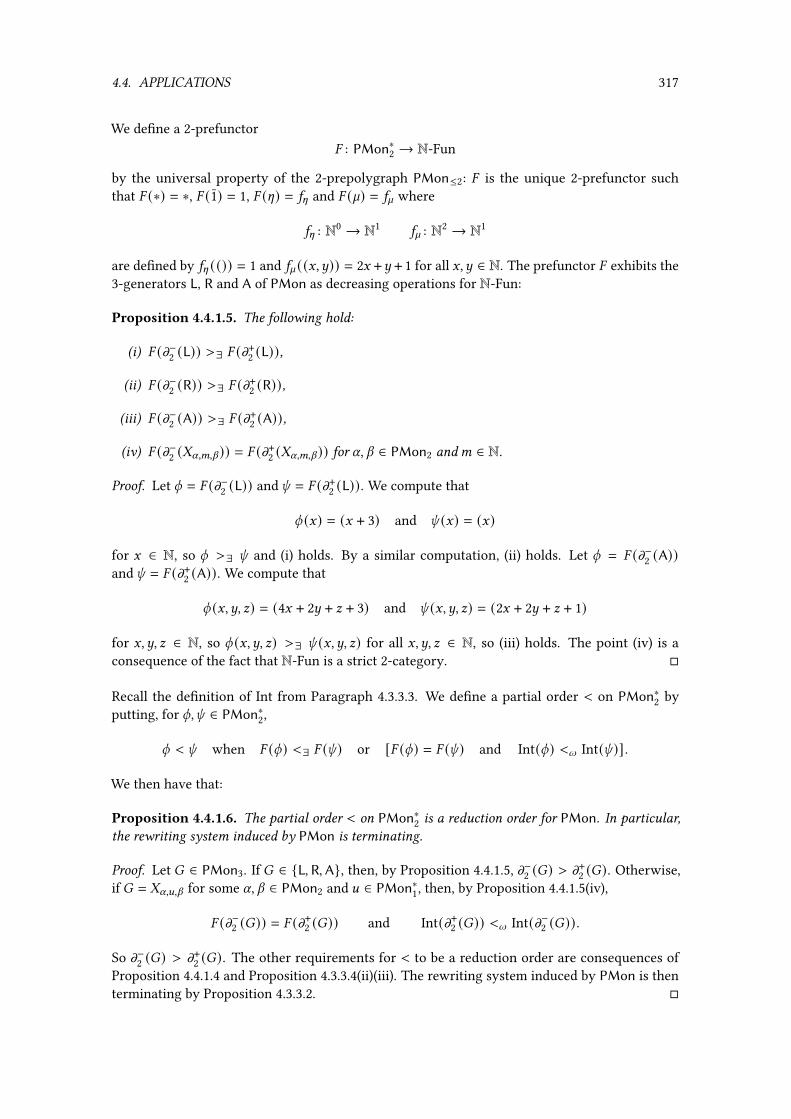
4.4. APPLICATIONS 317

We de�ne a 2-prefunctor� : PMon∗2 → N-Fun

by the universal property of the 2-prepolygraph PMon≤2: � is the unique 2-prefunctor suchthat � (∗) = ∗, � (1) = 1, � ([) = 5[ and � (`) = 5` where

5[ : N0 → N1 5` : N2 → N1

are de�ned by 5[ (()) = 1 and 5` ((G,~)) = 2G +~ + 1 for all G,~ ∈ N. The prefunctor � exhibits the3-generators L, R and A of PMon as decreasing operations for N-Fun:

Proposition 4.4.1.5. The following hold:

(i) � (m−2 (L)) >∃ � (m+2 (L)),

(ii) � (m−2 (R)) >∃ � (m+2 (R)),

(iii) � (m−2 (A)) >∃ � (m+2 (A)),

(iv) � (m−2 (-U,<,V )) = � (m+2 (-U,<,V )) for U, V ∈ PMon2 and< ∈ N.

Proof. Let q = � (m−2 (L)) andk = � (m+2 (L)). We compute that

q (G) = (G + 3) and k (G) = (G)

for G ∈ N, so q >∃ k and (i) holds. By a similar computation, (ii) holds. Let q = � (m−2 (A))andk = � (m+2 (A)). We compute that

q (G,~, I) = (4G + 2~ + I + 3) and k (G,~, I) = (2G + 2~ + I + 1)

for G,~, I ∈ N, so q (G,~, I) >∃ k (G,~, I) for all G,~, I ∈ N, so (iii) holds. The point (iv) is aconsequence of the fact that N-Fun is a strict 2-category. �

Recall the de�nition of Int from Paragraph 4.3.3.3. We de�ne a partial order < on PMon∗2 byputting, for q,k ∈ PMon∗2,

q < k when � (q) <∃ � (k ) or [� (q) = � (k ) and Int(q) <l Int(k )] .

We then have that:

Proposition 4.4.1.6. The partial order < on PMon∗2 is a reduction order for PMon. In particular,the rewriting system induced by PMon is terminating.

Proof. Let � ∈ PMon3. If � ∈ {L,R,A}, then, by Proposition 4.4.1.5, m−2 (�) > m+2 (�). Otherwise,if � = -U,D,V for some U, V ∈ PMon2 and D ∈ PMon∗1, then, by Proposition 4.4.1.5(iv),

� (m−2 (�)) = � (m+2 (�)) and Int(m+2 (�)) <l Int(m−2 (�)) .

So m−2 (�) > m+2 (�). The other requirements for < to be a reduction order are consequences ofProposition 4.4.1.4 and Proposition 4.3.3.4(ii)(iii). The rewriting system induced by PMon is thenterminating by Proposition 4.3.3.2. �

318 CHAPTER 4. COHERENCE FOR GRAY CATEGORIES

4.4.1.7 — Coherence. Since the rewriting system is terminating, we can conclude using ourcoherence criterion:

Theorem 4.4.1.8. PMon is a coherent Gray presentation.

Proof. By Proposition 4.4.1.6, the rewriting system induced by PMon is terminating. By Theo-rem 4.3.4.8, since '1, . . . , '5 ∈ PMon4, PMon is a coherent Gray presentation. �

Remark 4.4.1.9. The original de�nition of pseudomonoids of [SD97] uses a smaller set of 4-gene-rators for the presentation, namely {'1, '4}. Thus, the coherent presentations obtained usingTheorem 4.3.4.8 are not necessarily the smallest ones. The same situation happens in the settingof strict categories [GM09], where the presentation of pseudomonoids obtained through rewritinghas �ve 4-generators, whereas the common de�nition of pseudomonoids in strict 3-categoriesonly requires two 4-generators: MacLane’s pentagon, which is an analogue of '1 in strict cat-egories, and '4 (c.f. the de�nition of monoidal categories in Paragraph 1.5.1.1). Guiraud andMalbos shows that the equalities on the 3-cells associated with '2, '3, '5 can be recovered fromthe ones associated with '1 and '4. Their proof relies on the invertibility of the 3-cells, whichsuggests that '1 and '4 might not be su�cient for a coherent presentation of lax pseudomonoidexpressed in lax Gray categories, where the 3-cells L,R,A are not required to be invertible. Inthis lax context, it would be interesting to know whether the 4-generators '1, '2, '3, '4, '5 stillprovides su�cient equalities for a coherent presentation of lax pseudomonoids and, more gener-ally, whether rewriting techniques can be used to �nd coherent presentations in the context oflax Gray categories.

4.4.2 Pseudoadjunctions

We now show the coherence of the Gray presentation of pseudoadjunctions introduced below.The way we do this is again by using Theorem 4.3.4.8. However, we need a speci�c argument toshow the termination of the interchange generators on the associated rewriting system. For thispurpose, we introduce a notion of “connected” diagrams and use a result of [DV18] saying thatinterchange generators terminate on such connected diagrams.

4.4.2.1 — Gray presentation. We de�ne the 3-prepolygraph for pseudoadjunctions as the 3-pre-polygraph P such that

P0 = {x, y} P1 = {f : x→ y, g : y→ x} P2 = {[ : id1x ⇒ f r0 g, n : g r0 f ⇒ id1

y}

where [ and n are pictured as and respectively, and P3 is de�ned by P3 = {N, N}, where

N : ([ r0 f) r1 (f r0 n) V id2f and N: (g r0 [) r1 (n r0 b) V id2

g

which can be represented by

N : V and N: V .

We then extend P to a Gray presentation by adding 3-generators corresponding to interchangegenerators and 4-generators corresponding to independence generators and interchange natural-ity generators like we did for pseudomonoids in Example 4.2.3.3, following the de�nition of Graypresentation given in Paragraph 4.2.3.1. For coherence, we need to add other 4-generators to P4.Provided that P is terminating, by Theorem 4.3.4.8, it is enough to add 4-generators correspondingto the critical branchings.

4.4. APPLICATIONS 319

4.4.2.2 — Critical branchings. Using the constructive proof of Theorem 4.3.5.8, we compute allthe critical branchings of P. We then obtain, up to symmetrical branchings, two critical branchings

and .

We observe that each of these branchings is joinable, and we de�ne formal new 4-generators that�ll the holes:

'1 '2 .

We then de�ne PAdj as the Gray presentation obtained from P by adding '1 and '2 to P4.

4.4.2.3 — Connectedness. We now aim at showing that the associated rewriting system isterminating. However, we can not build a reduction order using Proposition 4.3.3.4 to handleinterchange generators, like for the case of pseudomonoids, since P is not positive. Instead, weinvoke the result of [DV18] that states the termination of interchange generators on “connected di-agrams”. Given a 2-prepolygraphQ , a 2-cell ofQ∗2 is connected when, intuitively, each 2-generatoron its graphical representation is accessible by a path starting from a top or bottom wire. For exam-ple, given the 3-prepolygraph Q such that Q0 = {∗}, Q1 = {1} and Q2 = { : 0⇒ 2, : 2⇒ 0},we can build the following two 2-cells of Q∗2

and

where the one on the left is connected whereas the one on the right is not, since the two 2-gene-rators of the “bubble” can not be accessed from the top or bottom border.

A more formal de�nition of connectedness can be obtained by computing the “connectedcomponents” of the diagram, together with a map between the top and bottom wires of thediagram to the associated connected components. This is adequatly represented by cospans of Set.Based on this idea, we de�ne a 2-precategory that allows to compute the connected componentsof the 2-cells of Q∗, for a 2-prepolygraph Q .

We de�ne the 2-precategory CoSpan as the 2-precategory

– which has a unique 0-cell, denoted ∗,

– whose 1-cells are the natural numbers, with 0 as identity and addition as composition,

– whose 2-cells< ⇒ = are the classes of equivalent cospans N∗< ( N∗=5 6

in Set,

where two cospans � ( �5 6

and � ( ′ �5 ′ 6′

are said equivalent when thereexists an isomorphism ℎ : ( → ( ′ ∈ Set such that 5 ′ = ℎ ◦ 5 and 6′ = ℎ ◦ 6. Given< ∈ CoSpan1,the identity id2

< ∈ CoSpan2 is the cospan

N∗< N∗< N∗<1N∗< 1N∗<

320 CHAPTER 4. COHERENCE FOR GRAY CATEGORIES

and, given 2-cells q : <1 ⇒<2 andk : <2 ⇒<3 of CoSpan, represented by the cospans

N∗<1 ( N∗<2

5 6and N∗<2 ( ′ N∗<3

5 ′ 6′

respectively, their composite is represented by the cospan

( ′′

( ( ′

N∗<1 N∗<2 N∗<3

ℎ ℎ′

5 6 5 ′ 6′

where the middle square is a pushout. Given q : < ⇒ = ∈ CoSpan2 represented by

N∗< ( N∗=5 6

and ?, @ ∈ CoSpan1, the 2-cell ? r0 q r0 @ is represented by the cospan

N∗? t ( t N∗@

N∗?+<+@ N∗?+=+@

(1N∗?t5 t1N∗@ )◦\?,<,@ (1N∗?t6t1N∗@ )◦\?,=,@

where \?,A,@ : N∗?+A+@ → N∗? t N∗A t N∗@ , for A ∈ N, is the evident bijection. By checking thecondition (E), one easily veri�es that CoSpan is in fact a strict 2-category.

Given a 2-prepolygraph Q , by the universal property of 2-prepolygraph, we de�ne a 2-prefunctor

ConQ : Q∗ → CoSpan

such that

– the image of G ∈ Q0 by ConQ is ∗,

– the image of 0 ∈ Q1 by ConQ is 1,

– the image of U : 5 ⇒ 6 ∈ Q2 by ConQ is represented by the unique cospan

N∗|5 | {∗} N∗|6 |∗ ∗ .

We can now give a formal de�nition for connectedness: a cell q ∈ Q∗2 is connected when ConQ (q)is represented by a cospan

N∗< ( N∗=5 6

with< = |m−1 (q) | and = = |m+1 (q) | such that 5 , 6 are jointly epimorphic. Since the latter propertyis invariant by equivalences of cospan, if q is connected, then for all representant

N∗< ( N∗=5 ′ 6′

of ConQ (q), 5 ′, 6′ are jointly epimorphic.

Connectedness is not changed by 3-generators that are similar to interchange generators, as aconsequence of the following property:

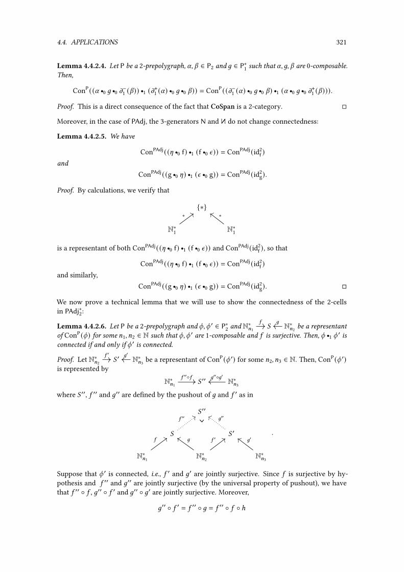
4.4. APPLICATIONS 321

Lemma 4.4.2.4. Let P be a 2-prepolygraph, U, V ∈ P2 and 6 ∈ P∗1 such that U,6, V are 0-composable.Then,

ConP((U r0 6 r0 m−1 (V)) r1 (m+1 (U) r0 6 r0 V)) = ConP((m−1 (U) r0 6 r0 V) r1 (U r0 6 r0 m+1 (V))).Proof. This is a direct consequence of the fact that CoSpan is a 2-category. �

Moreover, in the case of PAdj, the 3-generators N and Ndo not change connectedness:

Lemma 4.4.2.5. We have

ConPAdj(([ r0 f) r1 (f r0 n)) = ConPAdj(id2f )

and

ConPAdj((g r0 [) r1 (n r0 g)) = ConPAdj(id2g).

Proof. By calculations, we verify that

{∗}

N∗1 N∗1

∗ ∗

is a representant of both ConPAdj(([ r0 f) r1 (f r0 n)) and ConPAdj(id2f ), so that

ConPAdj(([ r0 f) r1 (f r0 n)) = ConPAdj(id2f )

and similarly,ConPAdj((g r0 [) r1 (n r0 g)) = ConPAdj(id2

g). �

We now prove a technical lemma that we will use to show the connectedness of the 2-cellsin PAdj∗2:

Lemma 4.4.2.6. Let P be a 2-prepolygraph and q, q ′ ∈ P∗2 and N∗=1 ( N∗=2

5 6be a representant

of ConP(q) for some =1, =2 ∈ N such that q, q ′ are 1-composable and 5 is surjective. Then, q r1 q ′ isconnected if and only if q ′ is connected.

Proof. Let N∗=2 ( ′ N∗=3

5 ′ 6′be a representant of ConP(q ′) for some =2, =3 ∈ N. Then, ConP(q ′)

is represented by

N∗=1 ( ′′ N∗=3

5 ′′◦5 6′′◦6′

where ( ′′, 5 ′′ and 6′′ are de�ned by the pushout of 6 and 5 ′ as in

( ′′

( ( ′

N∗=1 N∗=2 N∗=3

5 ′′ 6′′

5 6 5 ′ 6′.

Suppose that q ′ is connected, i.e., 5 ′ and 6′ are jointly surjective. Since 5 is surjective by hy-pothesis and 5 ′′ and 6′′ are jointly surjective (by the universal property of pushout), we havethat 5 ′′ ◦ 5 , 6′′ ◦ 5 ′ and 6′′ ◦ 6′ are jointly surjective. Moreover,

6′′ ◦ 5 ′ = 5 ′′ ◦ 6 = 5 ′′ ◦ 5 ◦ ℎ

322 CHAPTER 4. COHERENCE FOR GRAY CATEGORIES

where ℎ is a factorization of 6 through 5 (that exists, since 5 is supposed surjective). Thus, weconclude that 5 ′′ ◦ 5 and 6′′ ◦ 6 are jointly surjective.

Conversely, suppose that q r1 q ′ is connected, i.e., 5 ′′ ◦ 5 and 6′′ ◦ 6 are jointly surjective andlet ~ ∈ ( ′. We have to show that ~ is in the image of 5 ′ or 6′. Recall that

( ′′ ' ((∐

( ′)/∼

where ∼ is the equivalence relation induced by 6(G) ∼ 5 ′(G) for G ∈ N∗=2 so either~ is in the imageof 5 ′ or [~ is the only preimage of 6′′(~) by 6′′ and 6′′(~) is not in the image of 5 ′′]. In the formercase, we conclude directly, and in the latter, since 5 ′′ ◦ 5 and 6′′ ◦ 6′ are jointly surjective, thereis G ∈ N∗=3 such that 6′′ ◦ 6′(G) = 6′′(~), so that 6′(G) = ~, which is what we wanted. Thus, 5 ′and 6′ are jointly surjective, i.e., q ′ is connected. �

We can now prove our connectedness result for pseudoadjunctions:

Proposition 4.4.2.7. For every q ∈ PAdj∗2, q is connected.

Proof. Suppose by contradiction that it is not true and let # ∈ N be the smallest such that theset ( = {q ∈ PAdj∗2 | |q | = # and q is not connected} is not empty. Given q ∈ ( , let

(51 r0 U1 r0 ℎ1) r1 · · · r1 (5# r0 U# r0 ℎ# )be a decomposition of q .

Note that there is at least one 8 ∈ N∗#

such that U8 = n . Indeed, given 5 , ℎ ∈ PAdj∗1 such that 5 , [, ℎare 0-composable, a representant

N∗< ) N∗=D E

of ConQ (5 r0 [ r0 ℎ) has the property that E is an epimorphism. Since epimorphisms are stable bypushouts, given q ′ ∈ PAdj∗2 such that q ′ = (5 ′1 r0 [ r0 ℎ′1) r1 · · · r1 (5 ′: r0 [ r0 ℎ′: ) with 5 ′8 , ℎ

′8 ∈ PAdj

∗1

for 8 ∈ N∗:, a representant

N∗<′ ) ′ N∗

=′D′ E′

of ConPAdj(q ′) has the property that E ′ is an epimorphism (by induction on :), and in particular,q ′is connected. So let 80 be minimal such that there is q ∈ ( with U80 = n .

Suppose �rst that 80 = 1. Then, given a representant

N∗<1 )1 N∗<2

D1 E1

of ConPAdj(51 r0 U1 r0 ℎ1), we easily check that D1 is an epimorphism. By Lemma 4.4.2.6, we deducethat

(52 r0 U2 r0 ℎ2) r1 · · · r1 (5: r0 U: r0 ℎ: )is not connected, contradicting the minimality of # .

Thus 80 > 1. By the de�nition of 80, we have U80−1 = [. There are then di�erent cases dependingon |580−1 |:

– if |580−1 | ≤ |580 | − 2, then, since m+1 (580−1 r0 U80−1 r0 ℎ80−1) = m−1 (580 r0 U80 r0 ℎ80), we have

580 = 580−1 r0 m+1 ([) r0 6 and ℎ80−1 = 6 r0 m−1 (n) r0 ℎ80

4.4. APPLICATIONS 323

for some 6 ∈ PAdj∗1. By Lemma 4.4.2.4, we have

ConPAdj(([ r0 6 r0 m−1 (n)) r1 (m+1 ([) r0 6 r0 n)) = ConPAdj((m−1 ([) r0 6 r0 n) r1 ([ r0 6 r0 m+1 (n)))thus, by functoriality of ConPAdj, the morphism q ′ de�ned by

q ′ = (51 r0 U1 r0 ℎ1) r1 · · · r1 (580−2 r0 U80−2 r0 ℎ80−2)r1 (580−1 r0 6 r0 n r0 ℎ80) r1 (580−1 r0 [ r0 6 r0 ℎ80)r1 (580+1 r0 U80+1 r0 ℎ80+1) r1 · · · r1 (5: r0 U: r0 ℎ: )satis�es that ConPAdj(q) = ConPAdj(q ′). So q ′ is not connected, and the (80−1)-th 2-gene-rator in the decomposition of q ′ is n , contradicting the minimality of 80;

– if |580−1 | ≥ |580 | + 2, then the case is similar to the previous one;

– if |580−1 | = |580 | − 1, then, since ConPAdj(([ r0 f) r1 (f r0 n)) = ConPAdj(id2f ) by Lemma 4.4.2.5,

the 2-cell q ′ de�ned by

q ′ = (51 r0 U1 r0 ℎ1) r1 · · · r1 (580−2 r0 U80−2 r0 ℎ80−2)r1 (580+1 r0 U80+1 r0 ℎ80+1) r1 · · · r1 (5: r0 U: r0 ℎ: )satis�es ConPAdj(q) = ConPAdj(q ′) (by functoriality of ConPAdj), so that q ′ is not connected,contradicting the minimality of # ;

– if |580−1 | = |580 | + 1, then the situation is similar to the previous one, since, by Lemma 4.4.2.5,

ConPAdj((g r0 [) r1 (n r0 g)) = ConPAdj(id2g);

– �nally, the case |580−1 | = |580 | is impossible since

580−1 r0 m+1 (U80−1) r0 ℎ80−1 = 580r0 m−1 (U80) r0 ℎ80

andm+1 (U80−1) = f r0 g ≠ g r0 f = m−1 (U80) . �

4.4.2.8 — Termination. We are now able to prove the termination of the rewriting system:

Proposition 4.4.2.9. The rewriting system associated to PAdj is terminating.

Proof. Suppose by contradiction that there is a sequence (8 : q8 V q8+1 for 8 ∈ Nwith (8 rewritingstep in PAdj∗3. Since

|m−2 (N) | = |m−2 ( N) | = 2 and |m+2 (N) | = |m+2 ( N) | = 0,

if the inner 3-generator of (8 is N or N, for some 8 ∈ N, then |q8+1 | = |q8 | − 2. Since

m−2 (-U,5 ,V ) = m+2 (-U,5 ,V ) = 2

for 0-composable U ∈ PAdj2, 5 ∈ PAdj∗1, V ∈ PAdj2, it means that there is 80 ∈ N such that for 8 ∈ Nwith 8 ≥ 80, the inner generator of (8 is an interchanger. By [DV18, Theorem 16], there is noin�nite sequence of rewriting steps made of interchangers. Thus, by Proposition 4.4.2.7, thereis no in�nite sequence of rewriting steps whose inner 3-generator is an interchanger of PAdj,contradicting the existence of ((8)8∈N. Thus, PAdj is terminating. �

324 CHAPTER 4. COHERENCE FOR GRAY CATEGORIES

4.4.2.10 — Coherence. Finally, we can apply our coherence criterion and show that:

Theorem 4.4.2.11. PAdj is a coherent Gray presentation.

Proof. By Proposition 4.4.2.9, the rewriting system associated to PAdj is terminating. By Theo-rem 4.3.4.8, since '1, '2 ∈ PAdj4, the conclusion follows. �

4.4.3 Frobenius pseudomonoid

We now consider the example of Frobenius pseudomonoids [Str04] that categorify the classicalnotion of Frobenius algebras. Sadly, our methods do not apply to show the coherence of thefull structure since the units induce non-joinable critical branchings, so that we only considernon-unitary Frobenius pseudomonoids. Moreover, we were not able to show termination of theassociated rewriting system, so that our coherence result is assuming termination. We still presentthis partial example, hoping it might motivate the developments of termination arguments asfuture works. We refer to [DV16] for a more complete treatment of the coherence of Frobeniuspseudomonoids.

4.4.3.1 — Gray presentation. We de�ne the 3-prepolygraph P of non-unitary Frobenius pseu-domonoids as follows. We put

P0 = {∗} P1 = {1} P2 = {` : 2→ 1, n : 1→ 2}

where we write = for the composite 1 r0 · · · r0 1 of = copies of 1 for = ∈ N. We picture ` and nby and respectively, and we de�ne P3 by P3 = {N, N,A,Aco,M,Mco} where

N : V A : V M : V

N: V Aco : V Mco : V

As before, we then extend P to a Gray presentation by adding 3-generators corresponding to inter-change generators and 4-generators corresponding to independence generators and interchangenaturality generators.

4.4.3.2 — Critical branchings and coherence. Using the constructive proof of Theorem 4.3.5.8,we �nd nineteen critical branchings for the above Gray presentation, which induce nineteenassociated formal 4-generators '1, . . . , '19 shown on Figure 4.1. We then de�ne PFrob as the Graypresentation obtained from P by adding to P4 the above 4-generators '1, . . . , '19. Since we werenot able to show termination, we only conclude that:

Proposition 4.4.3.3. If the rewriting system associated to PFrob is terminating, then PFrob is acoherent Gray presentation.

Proof. This is a consequence of Theorem 4.3.4.8. �

4.4.4 Self-dualities

We now consider the last example of self-dualities, which is an untyped variant of the one ofSection 4.4.2. This example requires a special treatment since the underlying rewriting system isnot terminating, and, more fundamentally, the induces (3, 2)-Gray category is not expected to befully coherent. We show instead a partial coherence result by adapting the general methods ofSection 4.3.

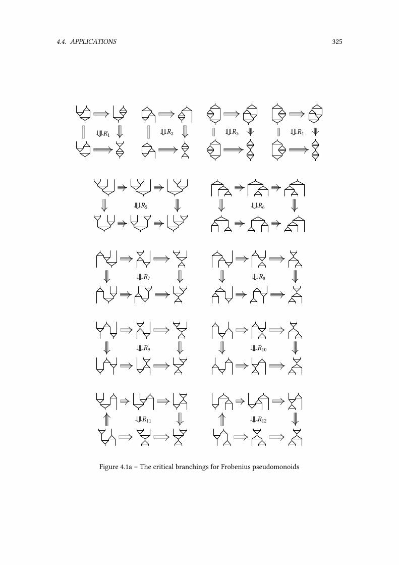
4.4. APPLICATIONS 325

'1 '2 '3 '4

'5 '6

'7 '8

'9 '10

'11 '12

Figure 4.1a – The critical branchings for Frobenius pseudomonoids

326 CHAPTER 4. COHERENCE FOR GRAY CATEGORIES

'13

'14 '15

'16 '17

'18 '19 .

Figure 4.1b – The critical branchings for Frobenius pseudomonoids

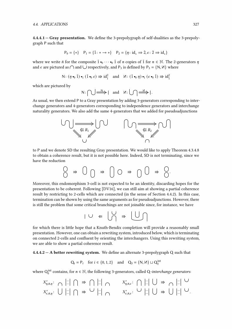
4.4. APPLICATIONS 327

4.4.4.1 — Gray presentation. We de�ne the 3-prepolygraph of self-dualities as the 3-prepoly-graph P such that

P0 = {∗} P1 = {1 : ∗ → ∗} P2 = {[ : id∗ ⇒ 2, n : 2⇒ id∗}

where we write = for the composite 1 r0 · · · r0 1 of = copies of 1 for = ∈ N. The 2-generators [and n are pictured as and respectively, and P3 is de�ned by P3 = {N, N} where

N : ([ r0 1) r1 (1 r0 n) V id21 and N: (1 r0 [) r1 (n r0 1) V id2

1

which are pictured byN : N and N: N .

As usual, we then extend P to a Gray presentation by adding 3-generators corresponding to inter-change generators and 4-generators corresponding to independence generators and interchangenaturality generators. We also add the same 4-generators that we added for pseudoadjunctions

'1 '2

to P and we denote SD the resulting Gray presentation. We would like to apply Theorem 4.3.4.8to obtain a coherence result, but it is not possible here. Indeed, SD is not terminating, since wehave the reduction

V V V V .

Moreover, this endomorphism 3-cell is not expected to be an identity, discarding hopes for thepresentation to be coherent. Following [DV16], we can still aim at showing a partial coherenceresult by restricting to 2-cells which are connected (in the sense of Section 4.4.2). In this case,termination can be shown by using the same arguments as for pseudoadjunctions. However, thereis still the problem that some critical branchings are not joinable since, for instance, we have

W V

for which there is little hope that a Knuth-Bendix completion will provide a reasonably smallpresentation. However, one can obtain a rewriting system, introduced below, which is terminatingon connected 2-cells and con�uent by orienting the interchangers. Using this rewriting system,we are able to show a partial coherence result.

4.4.4.2 — A better rewriting system. We de�ne an alternate 3-prepolygraph Q such that

Q8 = P8 for 8 ∈ {0, 1, 2} and Q3 = {N, N} t Q int3

where Q int3 contains, for = ∈ N, the following 3-generators, called Q-interchange generators:

- ′[,=,[ : V - ′[,=,n : V

- ′n,=,[ : V - ′n,=,n : V .

328 CHAPTER 4. COHERENCE FOR GRAY CATEGORIES

There is a 3-prefunctor Γ : Q∗ → P> uniquely de�ned by Γ(D) = D for 8 ∈ {0, 1, 2} and D ∈ Q∗8

and, for = ∈ N, mapping the 3-generators as follows:

N ↦→ N N↦→ N

- ′[,=,[ ↦→ -−1[,=,[ - ′[,=,n ↦→ -[,=,n

- ′n,=,[ ↦→ -−1n,=,n - ′n,=,n ↦→ -n,=,n .

We get a rewriting system (Q,==) by putting � == � ′ if and only if Γ(� ) = Γ(� ′) for parallel3-cells �, � ′ ∈ Q∗3 . Note that, given � : q V q ′ ∈ Q∗3 , the 2-cell q is connected if and only if q ′ isconnected. Indeed, one easily checks that for every � ∈ Q3, we have

ConQ (m−2 (�)) = ConQ (m+2 (�))

so that ConQ (q) = ConQ (q ′).

4.4.4.3 — Termination. We �rst show a weak termination property for Q , stating that it isterminating on connected 2-cells:

Proposition 4.4.4.4. Given a connected 2-cell q in Q∗2 , there is no in�nite sequence �8 : q8 V q8+1where q0 = q and �8 is a rewriting step for 8 ∈ N.

Proof. Since a rewriting step whose inner 3-generator is N or Ndecrease by two the number of2-generators in a diagram, it is enough to show that there is no in�nite sequence of composablerewriting steps made of elements of Q int

3 . Given a 2-cell q = (<1 r0 U1 r0 =1) r1 · · · r1 (<:r0 U: r0 =: )

of Q∗2 , with U8 ∈ Q2 and<8 , =8 ∈ N for 8 ∈ N∗:, we de�ne #1(q) ∈ N by

#1(q) = |{(8, 9) ∈ (N∗: )2 | 8 < 9 and U8 = [ and U 9 = n}|.

Moreover, if we write ?, @ ∈ N: and 81, . . . , 8? , 91, . . . , 9@ ∈ N∗: for the unique integers such that

81 < · · · < 8? 91 < · · · < 9@ {81, . . . , 8? , 91, . . . , 9@} = N∗:and U8A = [ and U 9B = n for A ∈ N∗? and B ∈ N∗@ , we de�ne #[2 (q) ∈ N? and # n

2 (q) ∈ N@ by

#[

2 (q) = (<8? , . . . ,<81) and # n2 (q) = (= 91, . . . , = 9@ ) .

Finally, we de�ne # (q) ∈ N1+?+@ by

# (q) = (#1(q), #[2 (q), #n2 (q))

and we equip N? , N@ and N1+?+@ with the lexicographical ordering <lex. Now, keeping q as above,let

_ r1 (; r0 � r0 A ) r1 d : q ⇒ q ′ ∈ Q∗3be a rewriting step for some ;, A ∈ Q∗1 , _, d, q ′ ∈ Q∗2 and � ∈ Q3 with

q ′ = (<′1 r0 U ′1 r0 =′1) r1 · · · r1 (<′: r0 U ′: r0 =′: )for some U ′8 ∈ Q2 and <′8 , =

′8 ∈ N for 8 ∈ N∗

:. If � = - ′[,D,n or � = - ′n,D,[ for some D ∈ N,

then #1(q ′) = #1(q) − 1.Otherwise, if � = -[,D,[ for some D ∈ N, then we have #1(q) = #1(q ′) and, writing A

for |_ | + 1, we have <B = <′B for B ∈ N∗:\ {A, A + 1}. Moreover, we have <′A+1 ≤ <A+1 − 2, so

that #[2 (q ′) <lex #[

2 (q).Otherwise, � = - ′n,D,n for some D ∈ N. Then #[2 (q) = #

[

2 (q ′) and, by a similar argument asbefore, # n

2 (q ′) <lex #n2 (q). In any case, we get that # (q) <lex # (q ′). Since <lex is well-founded,

we conclude that there is no in�nite sequence of rewriting steps '8 : q8 V q8+1 for 8 ∈ N with q0connected. �

4.4. APPLICATIONS 329

4.4.4.5 — Con�uence. We now aim at showing the con�uence of the branchings of Q . The ideais to use a critical pair lemma (Theorem 4.3.4.5) and a Newman’s lemma (Theorem 4.3.2.5) adaptedto the speci�c setting of Q where the notion of critical branching is di�erent and where we onlyconsider connected 2-cells as sources.

We say that a branching ((1, (2) of Q is connected when m−2 ((1) is connected. We say thatit is Q-critical when it is local, minimal, not trivial and not independent. We �rst state adaptedversions of the critical pair lemma and Newman’s lemma to the setting of Q:

Lemma 4.4.4.6. If all connected Q-critical branchings ((1, (2) of (Q,==) are con�uent, then allconnected local branchings of (Q,==) are con�uent.

Proof. By a direct adaptation of the proof of Theorem 4.3.4.5 to connected 2-cells and rewritingsteps between connected 2-cells. �

Lemma 4.4.4.7. If all connected local branchings of (Q,==) are con�uent, then all connected branch-ings of (Q,==) are con�uent.

Proof. By a direct adaptation of Theorem 4.3.2.5 to connected 2-cells and rewriting steps betweenconnected 2-cells, using Proposition 4.4.4.4. �

By the above properties, in order to deduce the con�uence of the branchings of Q , it is enough tocheck that the critical branchings of Q are con�uent, fact that we verify in the following property:

Lemma 4.4.4.8. The connected Q-critical branchings of (Q,==) are con�uent.

Proof. We �rst consider the Q-critical branchings ((1, (2) that are structural-structural, i.e., suchthat the inner 3-generators of (1 and (2 are Q-interchange generators. We classify them asseparated, half-separated and not separated. There are eight kinds of separated structural-structuralQ-critical branchings listed below:

(1) W V

(2) W V

(3) W V

(4) W V

(5) W V

(6) W V

(7) W V

(8) W V .

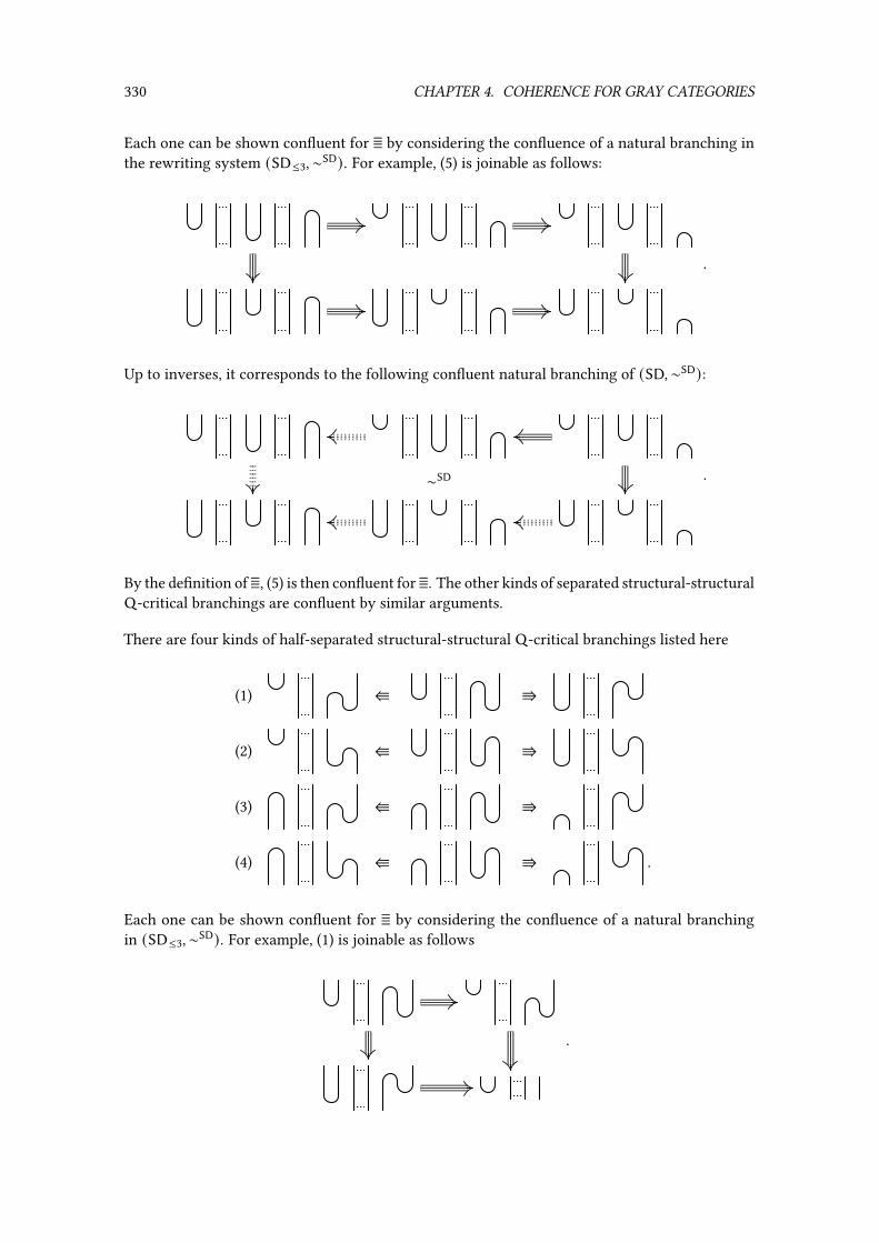
330 CHAPTER 4. COHERENCE FOR GRAY CATEGORIES

Each one can be shown con�uent for == by considering the con�uence of a natural branching inthe rewriting system (SD≤3,∼SD). For example, (5) is joinable as follows:

.

Up to inverses, it corresponds to the following con�uent natural branching of (SD,∼SD):

∼SD .

By the de�nition of ==, (5) is then con�uent for ==. The other kinds of separated structural-structuralQ-critical branchings are con�uent by similar arguments.

There are four kinds of half-separated structural-structural Q-critical branchings listed here

(1) W V

(2) W V

(3) W V

(4) W V .

Each one can be shown con�uent for == by considering the con�uence of a natural branchingin (SD≤3,∼SD). For example, (1) is joinable as follows

.

4.4. APPLICATIONS 331

Up to inverses, it corresponds to the following con�uent natural branching of (SD≤3,∼SD):

∼SD .

By de�nition of ==, it implies that (1) is con�uent for ==.

There are two kinds of not separated structural-structural Q-critical branchings listed below:

(1) W V

(2) W V

.

They are not con�uent but they are not connected branchings.We now consider structural-operational Q-critical branchings, i.e., those Q-critical branch-

ings ((1, (2) such that the inner 3-generator of (1 is a Q-interchange generator and the inner3-generator of (2 is N or N. We classify them as separated and half-separated. There are fourkinds of separated structural-operational Q-critical branchings listed below:

(1) W V

(2) W V

(3) W V

(4) W V .

Each one can be shown con�uent by considering a natural branching of (SD≤3,∼SD), like wasdone above.

There are two kinds of half-separated structural-operational Q-critical branchings listed below:

(1) W V

(2) W V .

As above, each one of them can be proved con�uent by considering the associated critical branch-ing in (SD≤3,∼SD).

Note that there are no operational-operational Q-critical branching, i.e., Q-critical branch-ings ((1, (2) where the inner 3-generators of both (1 and (1 are in {N, N}. Hence, all connectedQ-critical branchings are con�uent. �

332 CHAPTER 4. COHERENCE FOR GRAY CATEGORIES

We can conclude the following weak con�uence property:

Proposition 4.4.4.9. All the connected branchings of (Q,==) are con�uent.

Proof. By Lemmas 4.4.4.6 to 4.4.4.8. �

4.4.4.10 — Coherence. In order to obtain a weak coherence property for SD, we �rst state severaladapted versions of the properties of Section 4.3.1 to the setting of connected 2-cells:

Lemma 4.4.4.11. Given � : q V q ′ ∈ Q>3 where either q or q ′ is connected, we have � = � r2 �−1

for some � : q V k and � : q ′ V k .

Proof. By a direct adaptation of Proposition 4.3.1.3 involving connected 2-cells only, and usingProposition 4.4.4.9. �

Lemma 4.4.4.12. Given �1, �2 : q V q ′ ∈ Q3, if q is connected, then �1 = �2 in Q>3 .

Proof. Since q is connected, q ′ is connected. By Proposition 4.4.4.4, there is � : q ′ V k ∈ Q3such that k is a normal form for Q . By Proposition 4.4.4.9, there is �1, �2 : k V k ′ ∈ Q3 suchthat �1 r2 � r2 �1 = �1 r2 � r2 �2. Since k is a normal form, �1 = �2 = id

k. So �1 r2 � = �2 r2 � ,

thus �1 = �2 in Q>3 . �

Lemma 4.4.4.13. Given �1, �2 : q V q ′ ∈ Q>3 , if q is connected, then �1 = �2 in Q>3 .

Proof. By directly adapting the proof of Proposition 4.3.1.4, using Lemmas 4.4.4.11 and 4.4.4.12. �

We can now conclude with a weak coherence property for SD:

Theorem 4.4.4.14. Given �1, �2 : q V q ′ ∈ SD>3 with q or q ′ connected, we have �1 = �2.

Proof. Let Γ′ : Q> → SD> be the 3-prefunctor which is the factorization of Γ through the canoni-

cal 3-prefunctor (Q≤3)∗ → Q>. By de�nition of SD>, for 8 ∈ {1, 2}, we have

�8 = �8,1 r2 �−18,1

r2 · · · r2 �8,:8 r2 �−18,:8

for some :8 ∈ N, 2-cells q8,0, . . . , q8,:8 ,k8,1, . . . ,k8,:8 ∈ Q∗2 such that q8,0 = q and q8,:8 = q ′, and,for 9 ∈ N∗

:8, 3-cells

�8, 9 : q8, 9−1 V k8, 9 and �8, 9 : q8, 9 V k8, 9

of SD3. Since either q or q ′ is connected, we have that all the q8, 9 ’s and thek8, 9 ’s are connected.Moreover, all the �8, 9 ’s and the �8, 9 ’s are in the image of Γ′. So, for 8 ∈ {1, 2}, �8 = Γ′(� ′8 ) forsome � ′8 : q V q ′ ∈ Q>. By Lemma 4.4.4.13, we have � ′1 = �

′2, so that �1 = �2. �

Bibliography

[AR94] Jiří Adámek and Jiří Rosický. Locally Presentable and Accessible Categories. LondonMathematical Society Lecture Notes Series 189. Cambridge University Press, 1994.

[ABS00] Fahd A. Al-Agl, Ronald Brown, and Richard Steiner. Multiple categories: the equiva-lence of a globular and a cubical approach. 2000. arXiv: math/0007009.

[AM16] Dimitri Ara and Georges Maltsiniotis. Joint et tranches pour les l-catégories strictes.2016. arXiv: 1607.00668.

[AM18] Dimitri Ara and Georges Maltsiniotis. “Un théorème A de Quillen pour les∞-catégo-ries strictes I : la preuve simpliciale”. In: Advances in Mathematics 328 (2018), pp. 446–500.

[AK00] Chris J. Ash and Julia Knight. Computable Structures and the Hyperarithmetical Hier-archy. Studies in Logic and the Foundations of Mathematics 144. Elsevier, 2000.

[BN99] Franz Baader and Tobias Nipkow. Term Rewriting and All That. Cambridge UniversityPress, 1999.

[BS10] John Baez and Mike Stay. “Physics, topology, logic and computation: a Rosetta Stone”.In: New structures for physics. 2010, pp. 95–172.

[BKV16] Krzysztof Bar, Aleks Kissinger, and Jamie Vicary. “Globular: an online proof assistantfor higher-dimensional rewriting”. In: Leibniz International Proceedings in Informatics(LIPIcs). Vol. 52. 2016, 34:1–34:11. arXiv: 1612.01093.

[BV17] Krzysztof Bar and Jamie Vicary. “Data structures for quasistrict higher categories”.In: 32nd Annual Symposium on Logic in Computer Science (LICS). 2017, pp. 1–12. arXiv:1610.06908.

[Bat98a] Michael A. Batanin. “Computads for �nitary monads on globular sets”. In: Contem-porary Mathematics 230 (1998), pp. 37–58.

[Bat98b] Michael A. Batanin. “Monoidal globular categories as a natural environment for thetheory of weak =-categories”. In: Advances in Mathematics 136.1 (1998), pp. 39–103.

[Bec67] Jonathan M. Beck. “Triples, algebras and cohomology”. PhD thesis. Columbia Univer-sity, United States of America, 1967.

[Bén67] Jean Bénabou. “Introduction to bicategories”. In: Reports of the midwest category sem-inar. 1967, pp. 1–77.

333

334 BIBLIOGRAPHY

[Ber99] Clemens Berger. “Double loop spaces, braided monoidal categories and algebraic3-type of space”. In: Contemporary Mathematics 227 (1999), pp. 49–66.

[Bir84] Greg J. Bird. “Limits in 2-categories of locally-presented categories”. PhD thesis. Uni-versity of Sydney, Australia, 1984.

[Bor94a] Francis Borceux. Handbook of Categorical Algebra. Vol. 1: Basic Category Theory. En-cyclopedia of Mathematics and its Applications 50. Cambridge University Press, 1994.

[Bor94b] Francis Borceux. Handbook of Categorical Algebra. Vol. 2: Categories and Structures.Encyclopedia of Mathematics and its Applications 51. Cambridge University Press,1994.

[Bou07] Nicolas Bourbaki. Algèbre. Chapitres 1 à 3. Éléments de mathématique. Springer, 2007.[Buc15] Mitchell Buckley. “A formal veri�cation of the theory of parity complexes”. In: Journal

of Formalized Reasoning 8.1 (2015), pp. 25–48.[Bur93] Albert Burroni. “Higher-dimensional word problems with applications to equational

logic”. In: Theoretical Computer Science 115.1 (1993), pp. 43–62.[Bur12] Albert Burroni. “Automates et grammaires polygraphiques”. In:Diagrammes 67 (2012),

pp. 9–32.[Cam16] Alexander Campbell. “A higher categorical approach to Giraud’s non-abelian coho-

mology”. PhD thesis. Macquarie University, Australia, 2016.[Chu36] Alonzo Church. “An unsolvable problem of elementary number theory”. In: American

journal of mathematics 58.2 (1936), pp. 345–363.[CM17] Pierre-Louis Curien and Samuel Mimram. Coherent presentations of monoidal cate-

gories. 2017. arXiv: 1705.03553.[Deh11] Max Dehn. “Über unendliche diskontinuierliche Gruppen”. In: Mathematische An-

nalen 71 (1911), pp. 116–144.[DV18] Antonin Delpeuch and Jamie Vicary. Normalization for planar string diagrams and a

quadratic equivalence algorithm. 2018. arXiv: 1804.07832.[Dos18] Matěj Dostál. “Two-dimensional universal algebra”. PhD thesis. Czech Technical Uni-

versity in Prague, Czech Republic, 2018.[DV16] Lawrence Dunn and Jamie Vicary. Coherence for Frobenius pseudomonoids and the

geometry of linear proofs. 2016. arXiv: 1601.05372.[Ehr65] Charles Ehresmann. Catégories et structures. Dunod, 1965.[EM42] Samuel Eilenberg and Saunders MacLane. “Natural isomorphisms in group theory”.

In: Proceedings of the National Academy of Sciences of the United States of America28.12 (1942), p. 537.

[EM45] Samuel Eilenberg and Saunders MacLane. “General theory of natural equivalences”.In: Transactions of the American Mathematical Society 58.2 (1945), pp. 231–294.

[FM19] Simon Forest and Samuel Mimram. “Describing free l-categories”. In: 34th AnnualSymposium on Logic in Computer Science (LICS). 2019, pp. 1–13.

[GU06] Peter Gabriel and Friedrich Ulmer. Lokal präsentierbare Kategorien. Lecture Notes inMathematics 221. Springer, 2006.

[GGM15] Stéphane Gaussent, Yves Guiraud, and Philippe Malbos. “Coherent presentations ofArtin monoids”. In: Compositio Mathematica 151.5 (2015), pp. 957–998. arXiv: 1203.5358.

BIBLIOGRAPHY 335

[Göd34] Kurt Gödel. On undecidable propositions of formal mathematical systems. Notes byStephen C. Kleene and Barkely Rosser of lectures given at the Institute for AdvancedStudy. 1934.

[GPS95] Robert Gordon, A. John Power, and Ross Street. Coherence for Tricategories. Memoirsof the American Mathematical Society 558. American Mathematical Society, 1995.

[Gra06] John W. Gray. Formal Category Theory: Adjointness for 2-Categories. Lecture Notes inMathematics 391. Springer, 2006.

[Gue20] Léonard Guetta. “Polygraphs and discrete Conduchél-functors”. In:Higher Structures4.2 (2020).

[GM09] Yves Guiraud and Philippe Malbos. “Higher-dimensional categories with �nite deriva-tion type”. In: Theory and Applications of Categories 22.18 (2009), pp. 420–478.

[GM12] Yves Guiraud and Philippe Malbos. “Coherence in monoidal track categories”. In:Mathematical Structures in Computer Science 22.6 (2012), pp. 931–969.

[GM18] Yves Guiraud and Philippe Malbos. “Polygraphs of �nite derivation type”. In: Mathe-matical Structures in Computer Science 28.2 (2018), pp. 155–201. arXiv: 1402.2587.

[GMM13] Yves Guiraud, Philippe Malbos, and Samuel Mimram. “A homotopical completion pro-cedure with applications to coherence of monoids”. In: 24th International Conferenceon Rewriting Techniques and Applications (RTA). Vol. 21. 2013, pp. 223–238.

[Gur06] M. Nick Gurski. “An algebraic theory of tricategories”. PhD thesis. University ofChicago, United States of America, 2006.

[Gur13] M. Nick Gurski. Coherence in Three-Dimensional Category Theory. Cambridge Tractsin Mathematics 201. Cambridge University Press, 2013.

[Had18] Amar Hadzihasanovic.A combinatorial-topological shape category for polygraphs. 2018.arXiv: 1806.10353.

[Har98] Valentina S. Harizanov. “Pure computable model theory”. In: Studies in Logic and theFoundations of Mathematics 138. Elsevier, 1998, pp. 3–114.

[Hen17] Simon Henry. Non-unital polygraphs form a presheaf category. 2017. arXiv: 1711.00744.

[Hen18] Simon Henry. Regular polygraphs and the Simpson conjecture. 2018. arXiv: 1807 .02627.

[Jan84] Matthias Jantzen. “Thue systems and the Church-Rosser property”. In: InternationalSymposium on Mathematical Foundations of Computer Science. 1984, pp. 80–95.

[Joh87] Michael S. J. Johnson. “Pasting diagrams in =-categories with applications to coher-ence theorems and categories of paths”. PhD thesis. University of Sydney, Australia,1987.

[Joh89] Michael S. J. Johnson. “The combinatorics of =-categorical pasting”. In: Journal ofPure and Applied Algebra 62.3 (1989), pp. 211–225.

[Joy02] André Joyal. “Quasi-categories and Kan complexes”. In: Journal of Pure and AppliedAlgebra 175.1-3 (2002), pp. 207–222.

[JK06] André Joyal and Joachim Kock. Weak units and homotopy 3-types. 2006. arXiv: math/0602084.

[JS93] André Joyal and Ross Street. “Braided tensor categories”. In: Advances in Mathematics102.1 (1993), pp. 20–78.

336 BIBLIOGRAPHY

[KV91a] Mikhail Kapranov and Vladimir Voevodsky. “∞-groupoids and homotopy types”. In:Cahiers de Topologie et Géométrie Di�érentielle Catégoriques 32.1 (1991), pp. 29–46.

[KV91b] Mikhail Kapranov and Vladimir Voevodsky. “Combinatorial-geometric aspects ofpolycategory theory: pasting schemes and higher Bruhat orders (list of results)”. In:Cahiers de Topologie et Géométrie Di�érentielle Catégoriques 32.1 (1991), pp. 11–27.

[KS06] Masaki Kashiwara and Pierre Schapira.Categories and Sheaves. Grundlehren der math-ematischen Wissenschaften 332. Springer, 2006.

[Kel82] G. Max Kelly. Basic Concepts of Enriched Category Theory. London MathematicalSociety Lecture Notes Series 64. Cambridge University Press, 1982.

[Knu72] Donald E. Knuth. “Ancient babylonian algorithms”. In: Communications of the ACM15.7 (1972), pp. 671–677.

[Lac00] Stephen Lack. “A coherent approach to pseudomonads”. In: Advances in Mathematics152.2 (2000), pp. 179–202.

[Laf92] Yves Lafont. “Penrose diagrams and 2-dimensional rewriting”. In: Applications ofCategories in Computer Science 177 (1992), pp. 191–201.

[Laf95] Yves Lafont. “A new �niteness condition for monoids presented by complete rewritingsystems”. In: Journal of Pure and Applied Algebra 98.3 (1995), pp. 229–244.

[Laf03] Yves Lafont. “Towards an algebraic theory of boolean circuits”. In: Journal of Pureand Applied Algebra 184.2 (2003), pp. 257–310.

[Lei98] Tom Leinster. General operads and multicategories. 1998. arXiv: math/9810053.

[Lei04] Tom Leinster. Higher Operads, Higher Categories. London Mathematical Society Lec-ture Notes Series 298. Cambridge University Press, 2004.

[Mac63] Saunders MacLane. “Natural associativity and commutativity”. In: Rice UniversityStudies 49.4 (1963).

[Mac13] Saunders MacLane. Categories for the Working Mathematician. Graduate Texts inMathematics 5. Springer, 2013.

[MP85] Saunders MacLane and Robert Paré. “Coherence for bicategories and indexed cate-gories”. In: Journal of Pure and Applied Algebra 37 (1985), pp. 59–80.

[Mak05] Michael Makkai. The word problem for computads. 2005.

[MP89] Michael Makkai and Robert Paré. Accessible Categories: The Foundations of CategoricalModel Theory. Vol. 104. American Mathematical Society, 1989.

[Mar47] Andreï A. Markov. “Невозможность некоторых алгорифмов в теории ассоци-ативных систем (Impossibility of certain algorithms in the theory of associativesystems)”. In: Доклады Академии наук СССР 55 (1947), pp. 587–590.

[Mar97] Francisco Marmolejo. “Doctrines whose structure forms a fully faithful adjoint string”.In: Theory and Applications of Categories 3.2 (1997), pp. 24–44.

[Mét08] François Métayer. “Co�brant objects among higher-dimensional categories”. In: Ho-mology, Homotopy and Applications 10.1 (2008), pp. 181–203.

[Mim14] Samuel Mimram. “Towards 3-dimensional rewriting theory”. In: Logical Methods inComputer Science (LMCS) 10.1 (2014), pp. 1–47. arXiv: 1403.4094.

[Ngu17] Christopher Nguyen. “Parity structure on associahedra and other polytopes”. PhDthesis. Macquarie University, Australia, 2017.

BIBLIOGRAPHY 337

[Nov55] Pyotr S. Novikov. “Об алгоритмической неразрешимости проблемы тождестваслов в теории групп (On the algorithmic unsolvability of the word problem in grouptheory)”. In: Труды Математического института имени В.А. Стеклова СССР 44(1955), pp. 3–143.

[PV07] Erik Palmgren and Steven J. Vickers. “Partial Horn logic and cartesian categories”. In:Annals of Pure and Applied Logic 145.3 (2007), pp. 314–353.

[Pen99] Jacques Penon. “Approche polygraphique des∞-catégories non strictes”. In: Cahiersde Topologie et Géométrie Di�érentielle Catégoriques 40.1 (1999), pp. 31–80.

[Pos47] Emil L. Post. “Recursive unsolvability of a problem of Thue”. In: The Journal of Sym-bolic Logic 12.1 (1947), pp. 1–11.

[Pow91] A. John Power. “An=-categorical pasting theorem”. In: Category theory. 1991, pp. 326–358.

[Rog87] Hartley Rogers Jr. Theory of Recursive Functions and E�ective Computability. MITPress, 1987.

[Sim98] Carlos Simpson. Homotopy types of strict 3-groupoids. 1998. arXiv: math/9810059.[Sim11] Carlos Simpson. Homotopy Theory of Higher Categories. From Segal Categories to =-Ca-

tegories and Beyond. New Mathematical Monographs 19. Cambridge University Press,2011.

[Sko23] Thoralf Skolem. Begründung der elementaren Arithmetik durch die rekurrierende Denk-weise ohne Anwendung scheinbarer Veränderlichen mit unendlichem Ausdehnungsbere-ich. Dybusach, 1923.

[Squ87] Craig C. Squier. “Word problems and a homological �niteness condition for monoids”.In: Journal of Pure and Applied Algebra 49.1-2 (1987), pp. 201–217.

[SOK94] Craig C. Squier, Friedrich Otto, and Yuji Kobayashi. “A �niteness condition for rewrit-ing systems”. In: Theoretical Computer Science 131.2 (1994), pp. 271–294.

[Ste04] Richard Steiner. “Omega-categories and chain complexes”. In: Homology, Homotopyand Applications 6.1 (2004), pp. 175–200.

[Str72] Ross Street. “The formal theory of monads”. In: Journal of Pure and Applied Algebra2.2 (1972), pp. 149–168.

[Str76] Ross Street. “Limits indexed by category-valued 2-functors”. In: Journal of Pure andApplied Algebra 8.2 (1976), pp. 149–181.

[Str87] Ross Street. “The algebra of oriented simplexes”. In: Journal of Pure and AppliedAlgebra 49.3 (1987), pp. 283–335.

[Str91] Ross Street. “Parity complexes”. In: Cahiers de Topologie et Géométrie Di�érentielleCatégoriques 32.4 (1991), pp. 315–343.

[Str94] Ross Street. “Parity complexes: corrigenda”. In: Cahiers de Topologie et GéométrieDi�érentielle Catégoriques 35.4 (1994), pp. 359–361.

[Str96] Ross Street. “Categorical structures”. In: Handbook of Algebra. Vol. 1. 1996, pp. 529–577.

[Str04] Ross Street. “Frobenius monads and pseudomonoids”. In: Journal of MathematicalPhysics 45.10 (2004), pp. 3930–3948.

[SD97] Ross Street and Brian Day. “Monoidal bicategories and Hopf algebroids”. In: Advancesin Mathematics 129 (1997), pp. 99–157.

338 BIBLIOGRAPHY

[Ter03] Terese. Term Rewriting Systems. Cambridge Tracts in Theoretical Computer Science55. Cambridge University Press, 2003.

[Thu14] Axel Thue. “Probleme über Veränderungen von Zeichenreihen nach gegebenen Re-geln”. In: Christiana Videnskabs-Selskabs Skrifter: Mathematisk-naturwidenskabeligklasse. 10. 1914.

[Tur36] Alan M. Turing. “On computable numbers, with an application to the Entschei-dungsproblem”. In: Proceedings of the London Mathematical Society (2) 42.1 (1936),pp. 230–265.

[Tur37] Alan M. Turing. “Computability and _-de�nability”. In: The Journal of Symbolic Logic2.4 (1937), pp. 153–163.

[Web09] Mark Weber. Free products of higher operad algebras. 2009. arXiv: 0909.4722.

Index

activation, 216acyclic, 194adjunction, 20algebra over a monad, 10algebraic higher category, 2arity of a symbol, 5atom

of a pre-adc, 207of a pre-pasting scheme, 202of an l-hypergraph, 197

augmentation, 205augmented directed complex (adc), 205

basis of an adc, 205bicategory, 2boundary operator, 205branching, 301

cartesian monoidal structure, 78categorical action, 104:-category, 14category of elements, 175cell

of a :-category, 14of a (pre-)adc, 206of an l-hypergraph, 196

:-cellular extension, 40closed fgs, 202closed-well-formed, 244code

of a categorical action, 141of a cellular extension, 141of a function, 132

of a function w.r.t. encodings, 134of a globular set, 140of a precategory, 141of a strict category, 140relatively to an encoding, 134

co�nal functor, 17coherence cell, 2coherent

3-precategory, 299Gray presentation, 299

comparison functor, 11composable, 13, 268composition operation

for (pre-)adc cells, 207for l-hypergraph cells, 197for closed fgs’s, 243for maximal fgs’s, 243for pre-pasting scheme fgs’s, 203

computablecategorical action, 141cellular extension, 141globular set, 140polygraph, 152precategory, 140strict category, 140

computable function, 134concrete category, 174concrete presheaf category, 175concretely equivalent categories, 174concretization functor, 174Conduché functor, 116con�uent

339

340 INDEX

3-precategory, 299branching, 302rewriting system, 302

congruence, 274connected

2-cell, 320branching, 329category, 17

context (class), 106context (for a theory), 5convergent rewriting system, 302critical branching, 306Q-critical branching, 329

datatype, 135decidable

encoding, 134relation, 138subset, 133

diagram, 3direct loop, 202directed, 3

e�ectively factorizablecategorical action, 143precategory, 142strict category, 142

e�ectively right-�nite relation, 138Eilenberg-Moore category, 10encoded by a datatype, 135encoding, 134

of a cellular extension, 141of a globular set, 140

enriched category, 78equality-decidable encoding, 134equivalence of concrete categories, 174equivalent cospans, 319essentially algebraic

category, 7theory, 6

essentially unique factorization, 4evaluation

of a context (class), 106of a whisker, 267

evaluation of termsof precategories, 273strict categories, 155

exchange law, 58

�nitary

functor, 5monad, 5relation, 201

�niteclasses, 138polygraph, 51

�nite graded subset (fgs), 202�nitely factorizable

categorical action, 143precategory, 142strict category, 142

�nitely presentablemonoid, 4object, 4

fork-freefor an l-hypergraph, 194for an adc, 256for an adc cell, 256

free categoryon a cellular extension, 43on a polygraph, 47

free extension, 43Frobenius pseudomonoid, 324=-functor, 58funny tensor product, 79

generatorof a cellular extension, 40of a polygraph, 47of an l-hypergraph, 193

globe, 12globular algebra, 14=-globular group, 89globular set, 12glueable, 216gluing, 216graded set, 193Gray category, 283(3, 2)-Gray category, 284Gray presentation, 285greatest lower bound, 205=-group, 89

Henry’s measure, 99l-hypergraph, 193

identity context (class), 110identity operation

for (pre-)adc cells, 207for l-hypergraph cells, 197

INDEX 341

for closed or maximal fgs’s, 243for pre-pasting scheme fgs’s, 203

identity whisker, 269inclusion

of a globular algebra, 16of a globular set, 13of a strict category, 62of precategory, 68

independence generator, 285independent branching, 306initial set, 194injective encoding, 134inner generator, 301instantiable type, 106interchange generator, 285Q-interchange generator, 327interchange naturality generator, 286interchanger, 283iso�bration, 38

joinable branching, 301

labelling of a categorical action, 148lax Gray category, 283lax Gray tensor product, 282length

for a free precategory, 271for a free strict category, 123of an =-sequence, 122

linear extension, 225linearization of a category, 93local branching, 301localization functor, 276locally �nitely presentable category, 4loop-free basis, 208loop-free pasting scheme, 204

Makkai’s measure, 100maximal

fgs, 238generator, 238

maximal-well-formed, 244minimal branching, 306model of an essentially algebraic theory, 6monadic functor, 11monoidal category, 77morphism

of =-globular groups, 89of =-groups, 90of algebras, 10

of categorical actions, 105of enriched categories, 78of essentially algebraic theories, 8of globular sets, 12of lax Gray categories, 284of linear extensions, 225of models, 7of monads, 11of precategories, 67of set-encoded polygraphs, 157of strict categories, 58

movement, 196

natural branching, 306normal form, 301

operational generator, 312orthogonal, 214

parallel, 13parity complex, 198pasting scheme, 203plex, 176plex lifting, 181polygraph, 47

of precategories, 69of strict categories, 64

polyplex, 177polyplex lifting, 181positive

for a free abelian group, 99Gray presentation, 304

pre-augmented directed complex, 205pre-cell

of a (pre-)adc, 206of an l-hypergraph, 196

pre-pasting scheme, 201precategory, 66(3, 2)-precategory, 276=-prefunctor, 67prepolygraph, 69presentation (of precategories), 276primitive element, 175principal

element, 175polygraph, 176

pseudo Gray category, 284pseudo Gray tensor product, 282

radical, 257

342 INDEX

recursive function, 132recursive model

of a categorical action, 141of a cellular extension, 141of a function, 134of a globular set, 140of a precategory, 141of a strict category, 140

recursive subset, 133relevant, 197rewrite, 301rewriting path, 301rewriting step, 273rewriting system, 302right-�nite relation, 138

segment, 194self-duality, 324=-sequence, 122=-sequence class, 123set-encoded polygraph, 157signature, 5sort, 6source

for an l-hypergraph, 193iterated, 13of a closed fgs, 241of a context (class), 109of a globe, 12of a maximal fgs, 241of a pre-pasting scheme fgs, 202of a whisker, 268

source-�nite, 148specialization, 175split coequalizer, 59stable subset of a polygraph, 164strict category, 57structural-operational branching, 331structural-structural branching, 329support function, 162support of an encoding, 134symbol, 5symmetric branching, 301

targetfor an l-hypergraph, 193iterated, 13of a closed fgs, 241of a context (class), 109

of a globe, 12of a maximal fgs, 241of a pre-pasting fgs, 202of a symbol, 5of a whisker, 268

tensor product, 77term de�nition of a polygraph, 159term on a polygraph

of precategories, 273of strict categories, 155

term on a signature, 5terminal set, 194terminating, 301tight, 198torsion, 209torsion-free complex, 209total function, 131translation function, 239trivial branching, 305(weakly) truncable monad, 31truncation

of a globular algebra, 16of a globular set, 13of a strict category, 61of precategory, 68

type, 106

unital basis, 208

weird 2-category, 15well-formed fgs (wfs), 203well-typed term

of precategories, 273of strict categories, 155

whisker, 267word problem instance, 161word problem on polygraphs

of precategories, 273of strict categories, 156

zigzag (localization), 276zigzag equations (adjunctions), 20

Glossary

C) the Eilenberg-Moore category w.r.t. the monad ) . . . . . . . . . . . . . . . . . . . . . . . . . . . . . . . . . . 10Cq the functor derived from a morphism of monad q . . . . . . . . . . . . . . . . . . . . . . . . . . . . . . . . . 11-: ×8 -; the set of pairs of 8-composable :- and ;-globes . . . . . . . . . . . . . . . . . . . . . . . . . . . . . . 13-−1 by convention, the singleton set of (−1)-globes of a globular set . . . . . . . . . . . . . . . . . . . 13→,⇒,V, arrows which indicate the source and target of globes of a globular set . . . . 13(): , [: , `: ) the :-truncation of a monad ) on globular sets . . . . . . . . . . . . . . . . . . . . . . . . . . . . 14∼� the equivalence relation which describes how connected a category � is . . . . . . . . . . . . 17−[−]: , � [- ] the free functor which maps a :-cellular extension to a (:+1)-category . . . . 43(−)∗,: , P∗ the functor which maps a :-polygraph to the associated free :-category . . . . . . . 47(−):8 , P8 the functor which maps a :-polygraph to its set of 8-generators . . . . . . . . . . . . . . . . 48∗8 the composition operation for strict categories . . . . . . . . . . . . . . . . . . . . . . . . . . . . . . . . . . . . . 57r8 the composition operation for precategories . . . . . . . . . . . . . . . . . . . . . . . . . . . . . . . . . . . . . . . . 66� the funny tensor product . . . . . . . . . . . . . . . . . . . . . . . . . . . . . . . . . . . . . . . . . . . . . . . . . . . . . . . . . 79|−|, |� | the functor which maps an =-category to the disjoint union of the sets of cells . . . 93|−|, |P| the functor which maps a polygraph to the disjoint union of the sets of genera-

tors . . . . . . . . . . . . . . . . . . . . . . . . . . . . . . . . . . . . . . . . . . . . . . . . . . . . . . . . . . . . . . . . . . . . . . . . 97≈< the relation which witnesses that two<-contexts are equivalent . . . . . . . . . . . . . . . . . . . 106−[−]A, � [�]A the functor which maps an =-cellular extension to the associated free

=-categorical action . . . . . . . . . . . . . . . . . . . . . . . . . . . . . . . . . . . . . . . . . . . . . . . . . . . . . . . . . . 116�★ the set of =-sequences over � . . . . . . . . . . . . . . . . . . . . . . . . . . . . . . . . . . . . . . . . . . . . . . . . . . . . 122|D | the length of the cell D . . . . . . . . . . . . . . . . . . . . . . . . . . . . . . . . . . . . . . . . . . . . . . . . . . . . . . . . . . 122≈ the relation which witnesses that two =-sequences are equivalent . . . . . . . . . . . . . . . . . . . . 123�≈ the set of =-sequence classes over � . . . . . . . . . . . . . . . . . . . . . . . . . . . . . . . . . . . . . . . . . . . . . . 123−[−]≈, � [�]≈ the functor which maps an =-categorical action to the associated free

strict (=+1)-category . . . . . . . . . . . . . . . . . . . . . . . . . . . . . . . . . . . . . . . . . . . . . . . . . . . . . . . . 126◦:,(;8 )8 the composition operation on partial functions on natural numbers . . . . . . . . . . . . . . 131-<l the set of �nite sequences of elements of - . . . . . . . . . . . . . . . . . . . . . . . . . . . . . . . . . . . . . . 136⇑=A(- ) the trivial =-categorical action whose set of top cells is - . . . . . . . . . . . . . . . . . . . . . . . 148≈< a relation equivalent to ≈< but with a more e�cient de�nition . . . . . . . . . . . . . . . . . . . . . 153C1 ∗8,: C2 a term representing the 8-composition of C1 and C2 . . . . . . . . . . . . . . . . . . . . . . . . . . . . . 155È−ÉP the evaluation function from well-typed terms on P to cells of P∗ . . . . . . . . . . . . . . . . . 156� the polygraph induced by a term de�nition � . . . . . . . . . . . . . . . . . . . . . . . . . . . . . . . . . . . . . . 159PD+ the polygraph obtained from P by adding a formal generator of source D . . . . . . . . . . . . 178

343

344 GLOSSARY

(−)−, (−)+ the source and target operations of an l-hypergraph . . . . . . . . . . . . . . . . . . . . . . . 193⊳* , ⊳ a pre-order on the generators of an l-hypergraph . . . . . . . . . . . . . . . . . . . . . . . . . . . . . . . 194(−)∓, (−)± the border operations for sets of generators of an l-hypergraph . . . . . . . . . . . . . 195〈D〉 the atom associated to the generator D . . . . . . . . . . . . . . . . . . . . . . . . . . . . . . . . . . . . . . . . . . . 197(−)∓, (−)± the border operations on a pre-adc . . . . . . . . . . . . . . . . . . . . . . . . . . . . . . . . . . . . . . . . 205D ∧ E the greatest lower bound of D and E . . . . . . . . . . . . . . . . . . . . . . . . . . . . . . . . . . . . . . . . . . . . 205[D] the atom associated to the basis generator D of a pre-adc . . . . . . . . . . . . . . . . . . . . . . . . . . . 207<8 a pre-order on the basis of a pre-adc . . . . . . . . . . . . . . . . . . . . . . . . . . . . . . . . . . . . . . . . . . . . . . 208y a pre-order on the generators of an l-hypergraph . . . . . . . . . . . . . . . . . . . . . . . . . . . . . . . . . 212( ⊥ ) the property that ( and ) are orthogonal . . . . . . . . . . . . . . . . . . . . . . . . . . . . . . . . . . . . . . . 214∗M8 the composition operation on maximal fgs’s . . . . . . . . . . . . . . . . . . . . . . . . . . . . . . . . . . . . . . 243∗Cl8 the composition operation on closed fgs’s . . . . . . . . . . . . . . . . . . . . . . . . . . . . . . . . . . . . . . . . . 243PH the l-hypergraph associated to the polygraph P . . . . . . . . . . . . . . . . . . . . . . . . . . . . . . . . . . . 247∼� the canonical congruence on �≤= derived from the (=+1)-precategory � . . . . . . . . . . . . 274(−) the functor which maps an (=+1)-prepolygraph to the presented =-precategory . . . . . 276∼P the equivalence relation ∼P∗ . . . . . . . . . . . . . . . . . . . . . . . . . . . . . . . . . . . . . . . . . . . . . . . . . . . . . 276(−)> the localization functor of 3-precategories . . . . . . . . . . . . . . . . . . . . . . . . . . . . . . . . . . . . . . 276�lax the lax Gray tensor product . . . . . . . . . . . . . . . . . . . . . . . . . . . . . . . . . . . . . . . . . . . . . . . . . . . . . 278� the pseudo Gray tensor product . . . . . . . . . . . . . . . . . . . . . . . . . . . . . . . . . . . . . . . . . . . . . . . . . . . 282q �k the graph of the shu�es of words on q andk . . . . . . . . . . . . . . . . . . . . . . . . . . . . . . . . . . 286[−]q,k the interpretation functor for shu�es of words on q andk . . . . . . . . . . . . . . . . . . . . . . 287

Act(-,�) the activation of � on - . . . . . . . . . . . . . . . . . . . . . . . . . . . . . . . . . . . . . . . . . . . . . . . . . . 216adc “augmented directed complex” . . . . . . . . . . . . . . . . . . . . . . . . . . . . . . . . . . . . . . . . . . . . . . . . . . 205A: the functor which maps a :-cellular extension to its underlying :-algebra . . . . . . . . . . . 40Alg: the category of :-algebras . . . . . . . . . . . . . . . . . . . . . . . . . . . . . . . . . . . . . . . . . . . . . . . . . . . . . 14(−)Alg≤:,; , �≤: the truncation functor for globular algebras . . . . . . . . . . . . . . . . . . . . . . . . . . . . . . 16

(−)Alg↑;,: , �↑; the inclusion functor for globular algebras . . . . . . . . . . . . . . . . . . . . . . . . . . . . . . . . . 16

(−)Alg⇑=,: , �⇑= the right adjoint to the truncation functor (−)Alg

≤:,= . . . . . . . . . . . . . . . . . . . . . . . . . 35Alg+

:the category of :-cellular extensions . . . . . . . . . . . . . . . . . . . . . . . . . . . . . . . . . . . . . . . . . . . . 40

B the source relation of a pasting scheme . . . . . . . . . . . . . . . . . . . . . . . . . . . . . . . . . . . . . . . . . . . . 201

CatA= the category of =-categorical actions . . . . . . . . . . . . . . . . . . . . . . . . . . . . . . . . . . . . . . . . . . . 105(−)Cat≤:,; , �≤: the truncation functor for strict categories . . . . . . . . . . . . . . . . . . . . . . . . . . . . . . . . 61

(−)Cat↑;,: , �↑; the inclusion functor for strict categories . . . . . . . . . . . . . . . . . . . . . . . . . . . . . . . . . . 62

Cat= the category of strict =-categories . . . . . . . . . . . . . . . . . . . . . . . . . . . . . . . . . . . . . . . . . . . . . . 58Cat+= the category of =-cellular extension for strict categories . . . . . . . . . . . . . . . . . . . . . . . . . . 64V-Cat the category of categories enriched inV . . . . . . . . . . . . . . . . . . . . . . . . . . . . . . . . . . . . . . 79Cell∗( ) the set of cells of the pre-adc . . . . . . . . . . . . . . . . . . . . . . . . . . . . . . . . . . . . . . . . . . . . . 207Cell(%) the graded set of cells of the l-hypergraph % . . . . . . . . . . . . . . . . . . . . . . . . . . . . . . . . . 196Cell(%)=+ the strict (=+1)-category Cell(%)≤= [%=+1] . . . . . . . . . . . . . . . . . . . . . . . . . . . . . . . . . . 234Closed(%) the graded set of closed fgs’s of % . . . . . . . . . . . . . . . . . . . . . . . . . . . . . . . . . . . . . . . . . 238ClosedWF(%) the graded set of closed-well-formed fgs’s of the l-hypergraph % . . . . . . . . . 244ConP the evaluation prefunctor from P∗ to CoSpan . . . . . . . . . . . . . . . . . . . . . . . . . . . . . . . . . . . 320CoSpan the strict 2-category of cospans on sets . . . . . . . . . . . . . . . . . . . . . . . . . . . . . . . . . . . . . . 319

X� the linearization functor for a strict category � . . . . . . . . . . . . . . . . . . . . . . . . . . . . . . . . . . . . 96XP Henry’s measure . . . . . . . . . . . . . . . . . . . . . . . . . . . . . . . . . . . . . . . . . . . . . . . . . . . . . . . . . . . . . . . . 99

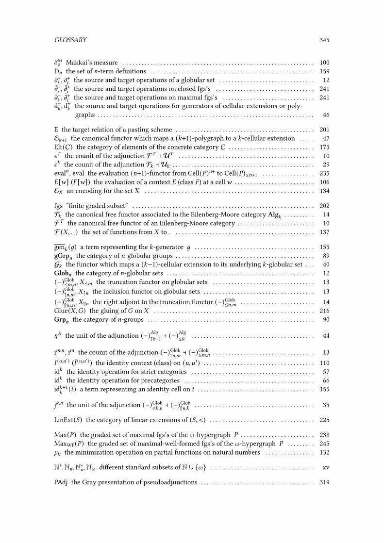
GLOSSARY 345

XMP Makkai’s measure . . . . . . . . . . . . . . . . . . . . . . . . . . . . . . . . . . . . . . . . . . . . . . . . . . . . . . . . . . . . . . 100

D= the set of =-term de�nitions . . . . . . . . . . . . . . . . . . . . . . . . . . . . . . . . . . . . . . . . . . . . . . . . . . . . . 159m−8 , m

+8 the source and target operations of a globular set . . . . . . . . . . . . . . . . . . . . . . . . . . . . . . . 12

m−8 , m+8 the source and target operations on closed fgs’s . . . . . . . . . . . . . . . . . . . . . . . . . . . . . . . . 241

m−8 , m+8 the source and target operations on maximal fgs’s . . . . . . . . . . . . . . . . . . . . . . . . . . . . . . 241

d−:, d+:

the source and target operations for generators of cellular extensions or poly-graphs . . . . . . . . . . . . . . . . . . . . . . . . . . . . . . . . . . . . . . . . . . . . . . . . . . . . . . . . . . . . . . . . . . . . . . 46

E the target relation of a pasting scheme . . . . . . . . . . . . . . . . . . . . . . . . . . . . . . . . . . . . . . . . . . . . . 201E:+1 the canonical functor which maps a (:+1)-polygraph to a :-cellular extension . . . . . 47Elt(C) the category of elements of the concrete category C . . . . . . . . . . . . . . . . . . . . . . . . . . . . 175n) the counit of the adjunction F) a U) . . . . . . . . . . . . . . . . . . . . . . . . . . . . . . . . . . . . . . . . . . . . 10n: the counit of the adjunction F: a U: . . . . . . . . . . . . . . . . . . . . . . . . . . . . . . . . . . . . . . . . . . . . . . 29eval= , eval the evaluation (=+1)-functor from Cell(%)=+ to Cell(%)≤=+1 . . . . . . . . . . . . . . . . . 235� [F] (� [F]) the evaluation of a context � (class � ) at a cellF . . . . . . . . . . . . . . . . . . . . . . . . . . 106E- an encoding for the set - . . . . . . . . . . . . . . . . . . . . . . . . . . . . . . . . . . . . . . . . . . . . . . . . . . . . . . . 134

fgs “�nite graded subset” . . . . . . . . . . . . . . . . . . . . . . . . . . . . . . . . . . . . . . . . . . . . . . . . . . . . . . . . . . . 202F: the canonical free functor associated to the Eilenberg-Moore category Alg: . . . . . . . . . . 14F) the canonical free functor of an Eilenberg-Moore category . . . . . . . . . . . . . . . . . . . . . . . . . 10F (-,. ) the set of functions from - to . . . . . . . . . . . . . . . . . . . . . . . . . . . . . . . . . . . . . . . . . . . . . . 137

gen: (6) a term representing the :-generator 6 . . . . . . . . . . . . . . . . . . . . . . . . . . . . . . . . . . . . . . . 155gGrp= the category of =-globular groups . . . . . . . . . . . . . . . . . . . . . . . . . . . . . . . . . . . . . . . . . . . . . 89G: the functor which maps a (:−1)-cellular extension to its underlying :-globular set . . . 40Glob= the category of =-globular sets . . . . . . . . . . . . . . . . . . . . . . . . . . . . . . . . . . . . . . . . . . . . . . . . 12(−)Glob≤<,= , -≤< the truncation functor on globular sets . . . . . . . . . . . . . . . . . . . . . . . . . . . . . . . . . 13

(−)Glob↑=,< , -↑= the inclusion functor on globular sets . . . . . . . . . . . . . . . . . . . . . . . . . . . . . . . . . . . . 13

(−)Glob⇑<,= , -⇑= the right adjoint to the truncation functor (−)Glob

≤=,< . . . . . . . . . . . . . . . . . . . . . . . . 14Glue(-,�) the gluing of � on - . . . . . . . . . . . . . . . . . . . . . . . . . . . . . . . . . . . . . . . . . . . . . . . . . . . . 216Grp= the category of =-groups . . . . . . . . . . . . . . . . . . . . . . . . . . . . . . . . . . . . . . . . . . . . . . . . . . . . . . 90

[A the unit of the adjunction (−)Alg↑:+1 a (−)

Alg≤: . . . . . . . . . . . . . . . . . . . . . . . . . . . . . . . . . . . . . . . . 44

i<,= , i< the counit of the adjunction (−)Glob↑=,< a (−)

Glob≤<,= . . . . . . . . . . . . . . . . . . . . . . . . . . . . . . . . . 13

� (D,D′) (� (D,D′) ) the identity context (class) on (D,D ′) . . . . . . . . . . . . . . . . . . . . . . . . . . . . . . . . . . . . 110

id: the identity operation for strict categories . . . . . . . . . . . . . . . . . . . . . . . . . . . . . . . . . . . . . . . . 57id: the identity operation for precategories . . . . . . . . . . . . . . . . . . . . . . . . . . . . . . . . . . . . . . . . . . 66id:+1:(C) a term representing an identity cell on C . . . . . . . . . . . . . . . . . . . . . . . . . . . . . . . . . . . . . . 155

j:,= the unit of the adjunction (−)Glob≤:,= a (−)

Glob⇑=,: . . . . . . . . . . . . . . . . . . . . . . . . . . . . . . . . . . . . . . . 35

LinExt(() the category of linear extensions of ((, <) . . . . . . . . . . . . . . . . . . . . . . . . . . . . . . . . . . 225

Max(%) the graded set of maximal fgs’s of the l-hypergraph % . . . . . . . . . . . . . . . . . . . . . . . . 238MaxWF(%) the graded set of maximal-well-formed fgs’s of the l-hypergraph % . . . . . . . . . 245`: the minimization operation on partial functions on natural numbers . . . . . . . . . . . . . . . . 132

N∗,N=,N∗=,Nl di�erent standard subsets of N ∪ {l} . . . . . . . . . . . . . . . . . . . . . . . . . . . . . . . . . . xv

PAdj the Gray presentation of pseudoadjunctions . . . . . . . . . . . . . . . . . . . . . . . . . . . . . . . . . . . . . 319

346 GLOSSARY

Part(-,. ) the set of partial functions from - to . . . . . . . . . . . . . . . . . . . . . . . . . . . . . . . . . . . . . 131(−)PCat≤:,; , �≤: the truncation functor for precategories . . . . . . . . . . . . . . . . . . . . . . . . . . . . . . . . . . 68

(−)PCat↑;,: , �↑; the inclusion functor for precategories . . . . . . . . . . . . . . . . . . . . . . . . . . . . . . . . . . . . 68

(−)PCat//=,=+1, �//= the left adjoint to the inclusion functor (−)PCat

↑=+1,= . . . . . . . . . . . . . . . . . . . . . . . 274PCat(E)= the category of precategories which satisfy the exchange condition (E) . . . . . . . . . 71PCat= the category of =-precategories . . . . . . . . . . . . . . . . . . . . . . . . . . . . . . . . . . . . . . . . . . . . . . . 67PCell∗( ) the set of pre-cells of the pre-adc . . . . . . . . . . . . . . . . . . . . . . . . . . . . . . . . . . . . . . . . 206PCell(%) the graded set of pre-cells of % . . . . . . . . . . . . . . . . . . . . . . . . . . . . . . . . . . . . . . . . . . . . . . 196PFrob the Gray presentation of non-unitary Frobenius pseudomonoids . . . . . . . . . . . . . . . . . 324Pf (- ) the set of �nite subsets of - . . . . . . . . . . . . . . . . . . . . . . . . . . . . . . . . . . . . . . . . . . . . . . . . . . 136PMon the Gray presentation of pseudomonoids . . . . . . . . . . . . . . . . . . . . . . . . . . . . . . . . . . . . . . 315Pol: the category of :-polygraphs . . . . . . . . . . . . . . . . . . . . . . . . . . . . . . . . . . . . . . . . . . . . . . . . . . . 47Poll the category of l-polygraphs . . . . . . . . . . . . . . . . . . . . . . . . . . . . . . . . . . . . . . . . . . . . . . . . . . 49Pol∗l the category Poll equipped with the concretization functor | (−)∗ | . . . . . . . . . . . . . . . . 175(−)Pol≤: , P≤: the truncation functor for polygraphs . . . . . . . . . . . . . . . . . . . . . . . . . . . . . . . . . . . . . 47

pre-adc “pre-augmented directed complex” . . . . . . . . . . . . . . . . . . . . . . . . . . . . . . . . . . . . . . . . . . . 205

R the closure relation for a pasting scheme or, more generally, an l-hypergraph . . . . . . . . 202Rec: the set of recursive functions with : arguments . . . . . . . . . . . . . . . . . . . . . . . . . . . . . . . . . 132d: the recursion operation on partial functions on natural numbers . . . . . . . . . . . . . . . . . . . . 131

S(- ) the l-hypergraph pre-cell associated to the adc pre-cell - . . . . . . . . . . . . . . . . . . . . . . . 261SD the Gray presentation of self-dualities . . . . . . . . . . . . . . . . . . . . . . . . . . . . . . . . . . . . . . . . . . . . 327sePol= the category of set-encoded =-polygraphs . . . . . . . . . . . . . . . . . . . . . . . . . . . . . . . . . . . . . 157Σ(- ) the adc pre-cell associated to the l-hypergraph pre-cell - . . . . . . . . . . . . . . . . . . . . . . . 260Σ= (() the adc element associated to a subset ( of the basis of the adc . . . . . . . . . . . . . . . . . . . 256S= (B) the set associated to an element of an adc with basis . . . . . . . . . . . . . . . . . . . . . . . . . . . . . 256suppP the support function for the polygraph P . . . . . . . . . . . . . . . . . . . . . . . . . . . . . . . . . . . . . . 162

TPCM ,TM

PC,TMCl,T

ClM ,T

PCCl ,T

ClPC translation functions between PCell(%), Max(%) and Max(%) . . 239

\= the recursive bijection from N= to N . . . . . . . . . . . . . . . . . . . . . . . . . . . . . . . . . . . . . . . . . . . . . . 134t: the natural transformation which describes the truncability of a monad on globular

sets . . . . . . . . . . . . . . . . . . . . . . . . . . . . . . . . . . . . . . . . . . . . . . . . . . . . . . . . . . . . . . . . . . . . . . . . 31T P the set of terms on the polygraph P . . . . . . . . . . . . . . . . . . . . . . . . . . . . . . . . . . . . . . . . . . . . . . 155

U: the forgetful functor associated to the Eilenberg-Moore category Alg: . . . . . . . . . . . . . . 14h: the universal function for recursive functions with : arguments . . . . . . . . . . . . . . . . . . . . . 132U) the canonical forgetful functor of an Eilenberg-Moore category . . . . . . . . . . . . . . . . . . . . 10

V: the forgetful functor from a (:+1)-algebra to a :-cellular extension . . . . . . . . . . . . . . . . . 40

Weird the category of weird 2-categories . . . . . . . . . . . . . . . . . . . . . . . . . . . . . . . . . . . . . . . . . . . . 15WF(%) the graded set of well-formed =-fgs’s (or =-wfs’s) on % . . . . . . . . . . . . . . . . . . . . . . . . . 203wfs “well-formed fgs” . . . . . . . . . . . . . . . . . . . . . . . . . . . . . . . . . . . . . . . . . . . . . . . . . . . . . . . . . . . . . . 203W= the set of =-word problem instances . . . . . . . . . . . . . . . . . . . . . . . . . . . . . . . . . . . . . . . . . . . . . 161WP the set of well-typed terms on the polygraph P . . . . . . . . . . . . . . . . . . . . . . . . . . . . . . . . . . . 155

X the exchange relation for the top cells of categorical actions . . . . . . . . . . . . . . . . . . . . . . . . . 123-U,6,V the interchange generator associated to U,6, V . . . . . . . . . . . . . . . . . . . . . . . . . . . . . . . . . . 285-q,k the interchanger of q andk . . . . . . . . . . . . . . . . . . . . . . . . . . . . . . . . . . . . . . . . . . . . . . . . . . . . 283

GLOSSARY 347

XF,F′ the arrow between the wordsF andF ′ in a shu�e graph . . . . . . . . . . . . . . . . . . . . . . . . 287

Z(−), Z� the linearization functor for strict categories . . . . . . . . . . . . . . . . . . . . . . . . . . . . . . . . 93

Titre : Descriptions calculatoires de catégories supérieures

Mots clés : catégories supérieures, catégories strictes, catégories de Gray, réécriture, problème du mot, diagrammes derecollement

Résumé : Les catégories supérieures sont des structuresalgébriques constituées de cellules de différentes dimen-sions et équipées d’opérations de composition. Elles onttrouvé plusieurs applications en mathématiques (en parti-culier, dans le domaine de la topologie algébrique) et eninformatique théorique. Ce sont des structures notoirementcomplexes, dont la manipulation est technique et sujette auxerreurs. Le but de cette thèse est d’introduire plusieurs ou-tils informatiques pour les variantes strictes et semi-strictesdes catégories supérieures qui facilitent l’étude de ces ob-jets. Afin de répresenter les catégories supérieures par desdonnées finies, de sorte que ces dernières puissent êtretransmises comme entrée à un programme, on utilise lastructure de polygraphe, initialement introduite par Streetet Burroni pour les catégories strictes, et généralisée parBatanin à toute théorie algébrique de catégorie supérieure,qui permet de présenter des catégories supérieures par dessystèmes de générateurs. Le premier problème abordé parcette thèse est celui du problème du mot sur les catégo-ries strictes, qui consiste à déterminer si deux composéesformelles de cellules d’une catégorie stricte représentent lamême cellule. On donne une solution implémentable et rela-tivement efficace pour ce problème en améliorant la procé-dure de décision initialement donnée par Makkai. Ensuite,nous traitons les formalismes pour les diagrammes de re-collement. Ces derniers permettent de représenter effica-

cement les cellules de catégories strictes en utilisant desstructures ensemblistes et pour lesquels une implémenta-tion efficace est désirable. On étudie en particulier les troisprincipaux formalismes qui ont été introduits jusqu’ici : lescomplexes de parité de Street, les schémas de recollementde Johnson et les complexes dirigés augmentés de Stei-ner. Notre étude révèle que les axiomatiques des deux pre-miers est défectueuse, ce qui motive l’introduction d’unenouvelle structure, appelée complexe sans torsion, dont lesaxiomes ont de bonnes propriétés et généralisent ceux desautres formalismes. On montre que cette nouvelle structureest adéquate pour représenter informatiquement les caté-gories strictes en en donnant une implémentation. Pour fi-nir, on considère le problème des présentations cohérentesde structures algébriques exprimées dans les catégoriesfaibles de dimension 3, ces dernières étant connues pourêtre équivalentes aux catégories de Gray. En s’inspirantd’un résultat important de Squier dans le context des mo-noïdes, on adapte les résultats classiques de la théorie dela réécriture au contexte des catégories de Gray et relionsla cohérence de présentations de catégories de Gray à laconfluence de branchements critiques d’un système de ré-écriture associé. Avec ce résultat, nous déduisons une pro-cédure semi-automatique pour produire des présentationscohérentes de catégories de Gray, et nous l’appliquons surplusieurs exemples.

Title: Computational Descriptions of Higher Categories

Keywords: higher categories, strict categories, Gray categories, rewriting, word problem, pasting diagrams

Abstract: Higher categories are algebraic structures con-sisting of cells of various dimensions equipped with no-tions of composition, which have found many applications inmathematics (algebraic topology in particular) and theoreti-cal computer science. They are notably complicated struc-tures whose manipulation is technical and error-prone. Thepurpose of this thesis is to introduce several computationaltools for strict and semi-strict variants of higher categoriesthat ease the study of these objects. In order to representhigher categories as finite data, so that they can be givenas input to a program, we use the structure of polygraph,initially introduced by Street and Burroni for strict categoriesand then generalized by Batanin to any algebraic theory ofhigher category, which allows presenting higher categoriesby means of systems of generators. The first problem tack-led by this thesis is then the one of the word problem onstrict categories, which consists in deciding whether two for-mal composites of cells of strict categories represent thesame cell. We give an implementable and relatively effi-cient solution for it by improving the decidability procedureinitially given by Makkai. Then, we turn to pasting diagramformalisms for strict categories, that enable to efficiently

represent cells of strict categories using set-like structuresand for which a reliable implementation is desirable. Weconsider the three main formalisms that have been intro-duced until now, namely Street’s parity complexes, John-son’s pasting schemes and Steiner’s augmented directedcomplexes. Our study reveals that the axiomatics of the firsttwo ones are defective, which motivates the introduction of anew structure, called torsion-free complexes, whose axiomshave nice properties and generalize those of the three otherformalisms. We also show that they are amenable to con-crete computation, by providing an implementation of those.Finally, we consider the problem of coherence of presen-tations of algebraic structures expressed in 3-dimensionalweak categories, the latter being known to be equivalent toGray categories. Taking inspiration from a celebrated resultgiven by Squier in the context of monoids, we adapt the clas-sical tools from rewriting theory to the setting of Gray cate-gories and relate the coherence of presentations of Graycategories to the confluence of the critical branchings of anassociated rewriting system. From this result, we deducea semi-automated procedure to find coherent presentationsof Gray categories that we apply on several examples.

Institut Polytechnique de Paris91120 Palaiseau, France