Computational AeroSciences Branch NASA Langley Research …€¦ · Bypass transition in...

Bypass transition in compressible boundary layers

Pedro Paredes, Meelan Choudhari, Fei Li & Chau-Lyan Chang

Computational AeroSciences BranchNASA Langley Research Center

6th Symp. on Global Flow Instability and ControlSep 28 - Oct 2, 2015, Hersonissos, Crete, GR

https://ntrs.nasa.gov/search.jsp?R=20160006616 2020-04-24T09:35:13+00:00Z

Motivation

Paths to transition1: The rule of transient growthThe non-normality of the NS equations cangive rise to transient energy amplification

The nonnormality of the system can give rise to transient energy amplification.

Even though we experience exponential decay for large times, the non-orthogonal superposition of eigenvectors can lead to short-time growth of energy.

Geometric interpretation:

23. September, 2014 ANADE

Geometric interpretation

Transient growth is a candidate mechanism forseveral cases of bypass transition wherein theroute to laminar-turbulent transition bypassesthe well-known paths to turbulence via modalinstabilities of the underlying laminar basicstate, for example:

I large bluntness cones,I spherical forebodies, ...

1M.V. Morkovin, E. Reshotko, and T. Herbert. “Transition in open flow systems - A reassessment”. In: Bull. Am. Phys.Soc. 39:1882 (1994).

Bypass transition in compressible boundary layers 1 / 21

Motivation

Large bluntness cones2Motivation

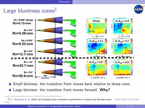
Large bluntness cones2

I n t e g r i t y - S e r v i c e - E x c e l l e n c e Approved for public release, distribution is unlimited.Distribution is unlimited, AEDC PA 2014-087

Model Configurations

10

7° Half-Angle

Reference Length: 1.55-m (5.1-ft)

Base Diameter: 0.381-m (15-in.)

Rn=0.15-mm

Rn=5.08-mm

Rn=9.53-mm

Rn=12.7-mm

Rn=25.7-mm

Rn=50.8-mm

I n t e g r i t y - S e r v i c e - E x c e l l e n c e Approved for public release, distribution is unlimited.Distribution is unlimited, AEDC PA 2014-087

Effect of Bluntness (Re/m ≈ 17×106)

ST/XSW ≈0.4 Delayed 2nd mode and increase length

for growth & breakdown Æ transition moves back vs. sharp

0.1< ST/XSW <0.3 Delayed 2nd mode; start of transition

precedes significant growth Ædifferent transition mechanism?

0.01< ST/XSW <0.07 No 2nd mode before start of transition; Me ≈ 3.3 at start of transition Transition mechanism is not known

Transient growth Entropy layer instability ???

24

Sharp ST/XSW ≈ 0.4

ST/XSW ≈ 0.3

ST/XSW ≈ 0.07 ST/XSW ≈ 0.02

ST/XSW ≈ 0.2

ST

Small blutness: the transition front moves back relative to sharp cone.Large blutness: the transition front moves forward. Why?

2E.C. Marineau et al. Mach 10 boundary-layer transition experiments on sharp and blunted cones. AIAA Paper 2014-3108.2014.


Small blutness: the transition front moves back relative to sharp cone.Large blutness: the transition front moves forward. Why?

2E.C. Marineau et al. Mach 10 boundary-layer transition experiments on sharp and blunted cones. AIAA Paper 2014-3108.2014.


Motivation

Spherical forebodies: the blunt body paradox3,4

Transition observed while the flow is T-S stable, Gortler stable (convexcurvature) and crossflow is negligible. Why?

2Note that images for Re=5.0E6/ft and Re=5.8E6/ft are interchanged.3E. Reshotko and A. Tumin. “The blunt body paradox - A case for transient growth”. In: Proc. of the IUTAM

Laminar-Turbulent Symposium V. ed. by H. Fasel and W. Saric. Sedona, AZ, USA, 2000, p. 403.4B.R. Hollis. Blunt-body entry vhicle aerothermodynamics: transition and turbulence on the CEV and MSL configurations.

AIAA Paper 2010-4984. 2010.Bypass transition in compressible boundary layers 3 / 21

Motivation

Can TG theory explain transition in these cases?7

Reshotko and Tumin5 suggested transient growth as a possible explanationfor transition over blunt nose tips and showed that a transition criterionbased on linear optimal growth provided successful correlation with thePANT database (M ≤ 6).Recent data6 corresponds to higher Mach numbers (M ≥ 6).

Current ongoing work:supersonic and hypersonic Mach numbers

nonlinear effects (nonlinear streak development, streak instabilities, interactionwith boundary layer instabilities, ...)

spatial approach including non-parallel effects

realistic geometries5E. Reshotko and A. Tumin. “Role of Transient Growth in Roughness-Induced Transition”. In: AIAA J. 42 (2004),

pp. 766–770.6E.C. Marineau et al. Mach 10 boundary-layer transition experiments on sharp and blunted cones. AIAA Paper 2014-3108.

2014.7P. Paredes et al. Transient growth analysis of compressible boundary layers with parabolized stability equations. (Submitted

to SciTech 2016). 2016.Bypass transition in compressible boundary layers 4 / 21

Summary

Zero-pressure-gradient flat plate BL at Mach 3Linear optimal disturbances

I Verification against prior results using self-similar base flow solutionI Extension to N-S base flow solution including leading edge shock

Non-linear evolution of finite-amplitude linearly optimal disturbancesInstability analysis of the perturbed flow

Examples of supersonic/hypersonic vehicles with flat plate components:

BOEING X-51A (Mach 5)8 NASA X-43A (Mach 10)9

8http://www.wpafb.af.mil/news/story.asp?id=1233469709http://www.nasa.gov/missions/research/x43-main.html


Theory

Transient growth analysis using PSE10

The optimal initial disturbance, q0, is defined as the inflow condition at x0that leads to maximum energy amplification or gain, G , up to a specifiedposition, x1.Objective function: J(q) = G = E(x1)

E(x0) .Mack’s energy norm: E (ξ) =

∫Ω q(x)HMq(x) dΩ, with

M = diag[

T (x)γρ(x)M2 , ρ(x), ρ(x), ρ(x), ρ(x)

γ(γ − 1)T (x)M2

].

Variational formulation using direct and adjoint PSE,

L(q, q∗) = J(q)− 〈q∗,Lq〉,

where q∗ denotes the vector of adjoint disturbance variables.The PSE approach allows the analysis of a broader class of mean flowsincluding those based on NS solvers.

10J.O. Pralits et al. “Optimal disturbances in three-dimensional boundary-layer flows”. In: Ercoftac Bull. 74 (2007),pp. 23–31.


Theory

Non-linear development of optimal perturbationsThe linearly optimal disturbance is used as inflow condition with finiteamplitude.The nonlinear-perturbation form of the parabolized Navier-Stokes equationsare used, which is equivalent to the nonlinear plane-marching PSE11 for asingle stationary perturbation (N = 0, α0 = 0):

q(x , y , z , t) =N∑

n=−Nqn(x , y , z) exp

[i∫

xαn(x ′)dx ′ − inωt

],

An implicit marching technique is used to facilitate the computation ofnonlinear streaks with large amplitudes.The instability of the resulting modified boundary layer flow is investigatedby the linear form of the plane-marching PSE12.

11P. Paredes et al. “The nonlinear PSE-3D concept for transition prediction in flows with a single slowly-varying spatialdirection”. In: Procedia IUTAM 14C (2015), pp. 35–44.

12P. Paredes. “Advances in global instability computations: from incompressible to hypersonic flow”. PhD thesis.Universidad Politecnica de Madrid, 2014.


Results Optimal disturbances in flat plate boundary layers

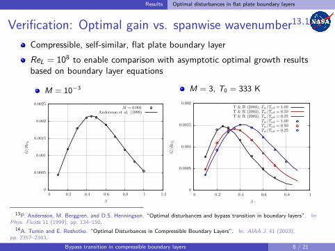
Verification: Optimal gain vs. spanwise wavenumber13,14

Compressible, self-similar, flat plate boundary layerReL = 108 to enable comparison with asymptotic optimal growth resultsbased on boundary layer equations

M = 10−3

0

0.0005

0.001

0.0015

0.002

0.0025

0 0.2 0.4 0.6 0.8 1 1.2

G/Re L

β

M = 0.001Andersson et al. (1999)

M = 3, T0 = 333 K

0

0.0005

0.001

0.0015

0.002

0 0.2 0.4 0.6 0.8 1

G/Re L

β

T & R (2003), Tw/Tad = 1.00T & R (2003), Tw/Tad = 0.50T & R (2003), Tw/Tad = 0.25

Tw/Tad = 1.00Tw/Tad = 0.50Tw/Tad = 0.25

13P. Andersson, M. Berggren, and D.S. Henningson. “Optimal disturbances and bypass transition in boundary layers”. In:Phys. Fluids 11 (1999), pp. 134–150.

14A. Tumin and E. Reshotko. “Optimal Disturbances in Compressible Boundary Layers”. In: AIAA J. 41 (2003),pp. 2357–2363.


Results Optimal disturbances in a Mach 3 flat plate boundary layer

Self-similar vs. full Navier-Stokes solutionsOptimal perturbations are commonly computed from the leading edge,x0 = 0, using the self-similar base flow solution, which ignores both theviscous-inviscid interaction near the leading edge and the weak shock waveemanating from that regionTo assess the effects of this simplification, a realistic basic state based onthe Navier-Stokes (NS) equations is used

NS parameters: Rn = 1 µm,Re′ = 106/m, T0 = 333 K, Tw/Tad = 1

Self-similar vs. NS b.l. profiles(R =

√xU/ν)

0

2

4

6

8

10

12

14

16

0 0.5 1 1.5 2 2.5 3

η=y/√ xν

/U∞

u/U∞, T /T∞

u/U∞, SST /T∞, SS

R = 20, u/U∞, NSR = 20, T /T∞, NSR = 100, u/U∞, NSR = 100, T /T∞, NSR = 316, u/U∞, NSR = 316, T /T∞, NSR = 1000, u/U∞, NSR = 1000, T /T∞, NS


Results Optimal disturbances in a Mach 3 flat plate boundary layer

Effect of initial optimization position, x0The final optimization position is R1 =

√x1U/ν = 1000 with x1 = L = 1 m,

which is used as reference length

Optimal gain using NS base flow

0

0.0005

0.001

0.0015

0.002

0.0025

0 0.2 0.4 0.6 0.8 1

G/Re L

β

x0 = 0.0004x0 = 0.01x0 = 0.04x0 = 0.09x0 = 0.16x0 = 0.25x0 = 0.36

Self-similar vs. NS results

0.0012

0.0014

0.0016

0.0018

0.002

0.0022

0.0024

0 0.05 0.1 0.15 0.2 0.25 0.3 0.35 0.4G/Re L

x0

β = 0.20, NSβ = 0.20, SSβ = 0.25, NSβ = 0.25, SSβ = 0.30, NSβ = 0.30, SS

Optimal β = 0.25 for inflow location at the leading edgeThe overall maximum G/ReL is found for x0 = 0.25 and β = 0.30As expected, the optimal G/ReL results using self-similar and NS base flows agreefor x0 > 0.25, while there is up to 10% deviation for x0 closer to the leading edge


Results Non-linear development of optimal disturbances

Non-linear evolution of streaks initiated near x0 = 0R0 =

√x0U/ν = 20 and β = 0.25

Initial amplitudes defined as A0 =√

E0 = A/√

Gmax with Gmax = 2398Streak amplitude based on u:Asu(x) = [maxy ,z (u(x , y , z))−miny ,z (u(x , y , z))] /2

Streak amplitude, Asu

0

0.1

0.2

0.3

0.4

0.5

0.6

0.7

0 500 1000 1500 2000

As u

R =√xU/ν

A = 0.10.51.02.03.04.05.010.015.0

Energy gain, G = E/E0

0

500

1000

1500

2000

2500

3000

0 500 1000 1500 2000

E/E

0

R =√xU/ν

Linear



Structure of streaks during non-linear evolution


0

0.1

0.2

0.3

0.4

0.5

0.6

0.7

0 500 1000 1500 2000

As u

R =√xU/ν

A = 0.10.51.02.03.04.05.010.015.0

A = 3 A = 10

u

0.95

0.9

0.85

0.8

0.75

0.7

0.65

0.6

0.55

0.5

0.45

0.4

0.35

0.3

0.25

0.2

0.15

0.1

0.05



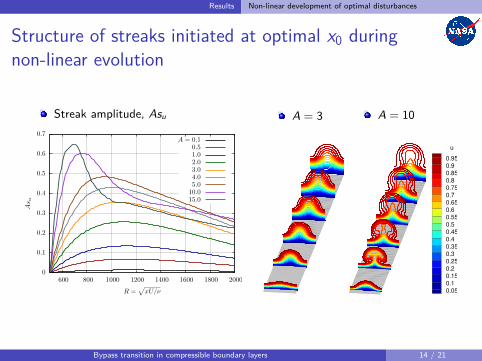
Non-linear streaks initiated at optimal x0

R0 =√

x0U/ν = 500 and β = 0.30


0

0.1

0.2

0.3

0.4

0.5

0.6

0.7

600 800 1000 1200 1400 1600 1800 2000

As u

R =√xU/ν

A = 0.10.51.02.03.04.05.010.015.0

Streak amplitude, Asu, for x0 → 0

0

0.1

0.2

0.3

0.4

0.5

0.6

0.7

0 500 1000 1500 2000

As u

R =√xU/ν

A = 0.10.51.02.03.04.05.010.015.0



Structure of streaks initiated at optimal x0 duringnon-linear evolution


0

0.1

0.2

0.3

0.4

0.5

0.6

0.7

600 800 1000 1200 1400 1600 1800 2000

As u

R =√xU/ν

A = 0.10.51.02.03.04.05.010.015.0

A = 3 A = 10

u

0.95

0.9

0.85

0.8

0.75

0.7

0.65

0.6

0.55

0.5

0.45

0.4

0.35

0.3

0.25

0.2

0.15

0.1

0.05


Results Instability analysis of the perturbed BL flow

Instability of streaks initiated at the leading edgeR0 =

√x0U/ν = 20 and β = 0.25

Spatial PDE based analysis at the final optimization position, R1 = 1000Two types of shear layer modes become unstable, the sinuous (S) and thevaricose (V) modes

Growth rate, −αi , vs. frequency, ω

-0.005

0

0.005

0.01

0.015

0.02

0 0.05 0.1 0.15 0.2 0.25

−αi

ω

A = 6, SA = 6, VA = 5, SA = 5, VA = 4, SA = 3, SA = 2, S

Sinuous,A = 6,ω = 0.115

0 0.01 0.020

0.005

0.01

0.015

0.02

u

0 0.01 0.020

0.005

0.01

0.015

0.02

T

Varicose,A = 6,ω = 0.0958

0 0.01 0.020

0.005

0.01

0.015

0.02

u

0 0.01 0.020

0.005

0.01

0.015

0.02

T


Results Instability analysis of the perturbed BL flow

Amplitude evolution of streak instabilities

R0 =√

x0U/ν = 20 and β = 0.25Plane-marching PSE analysis of the sinuous modeN-factor based on Mack’s energy norm

A = 3

0

2

4

6

8

10

600 800 1000 1200 1400 1600 1800 2000 2200

NE

R =√xU/ν

ω = 0.024ω = 0.048ω = 0.072ω = 0.096ω = 0.120ω = 0.144

A = 5

0

5

10

15

20

25

30

600 800 1000 1200 1400 1600 1800 2000 2200

NE

R =√xU/ν

ω = 0.024ω = 0.048ω = 0.072ω = 0.096ω = 0.120ω = 0.144ω = 0.168


Results Bypass transition in a Mach 3 flat plate BL

Natural transition in the unperturbed BL without streaksTransition prediction based on NE = 9 and 10Oblique first mode NE computed by linear PSE

N-factors based on E

0

2

4

6

8

10

12

14

16

1000 2000 3000 4000 5000 6000

NE

R =√xU/ν

β = 0.025β = 0.030β = 0.035β = 0.040β = 0.045β = 0.050

Transition location, Rex = R2

0

2e+06

4e+06

6e+06

8e+06

1e+07

0 0.0002 0.0004 0.0006 0.0008 0.001

Re x

=xU/ν

E0 = 2LzE0

First mode, N = 10First mode, N = 9

N = 10: Rex = 1.0417× 107, β = 0.040, ω ≈ 0.012N = 9: Rex = 8.3625× 106, β = 0.045, ω ≈ 0.012


Results Bypass transition in a Mach 3 flat plate BL

Bypass transition in a Mach 3 flat plate BLTransition prediction based on NE = 9 and 10Sinuous mode NE computed by linear plane-marching PSE

Asu vs. E0 = 2/Lz E0

0.01

0.1

1

1e-07 1e-06 1e-05 0.0001 0.001 0.01

As u

,max,As u

,R=1000

E0 = 2Lz

E0

Asu,max, R0 = 500Asu,R=1000, R0 = 500

Linear, R0 = 500Asu,max, R0 = 20

Asu,R=1000, R0 = 20Linear, R0 = 20

Transition location, Rex = R2

0

2e+06

4e+06

6e+06

8e+06

1e+07

0 0.0002 0.0004 0.0006 0.0008 0.001

Re x

=xU/ν

E0 = 2LzE0

First mode, N = 10First mode, N = 9R0 = 500, N = 10R0 = 500, N = 9R0 = 20, N = 10R0 = 20, N = 9

R0 = 20: β = 0.25, ω = 0.075− 0.100R0 = 500: β = 0.30, ω = 0.075− 0.100Oblique first mode: β = 0.040− 0.045, ω ≈ 0.012


Summary and Conlusions

Verification of newly developed linear, adjoint-PSE based optimization codefor compressible flows with results from literature.The effects of the viscous-inviscid interaction near the leading edge and theweak shock wave produce a 10% deviation from results based on self-similarbase flow when the initial optimization position is located near the leadingedge.Sinuous mode becomes unstable before the varicose mode for the moderateamplitude streaks studied.A non-linear perturbation form of the parabolized Navier-Stokes equations isdemonstrated for the computation of the downstream development ofhigh-amplitude stationary disturbances.The optimal initial optimization position for maximum energy also leads toearlier/stronger growth of secondary instability and, hence, earlier onset ofbypass transition relative to other inflow locations.Bypass transition via finite-amplitude optimal disturbances is demonstratedfor a zero-pressure-gradient flat plate boundary layer.


Extra charts

Instability of streaks initiated at the optimal x0R0 =

√x0U/ν = 500 and β = 0.30

Spatial PDE based analysis at the final optimization position, R1 = 1000Two types of shear layer modes become unstable, the sinuous (S) and thevaricose (V) modes

Growth rate, −αi , vs. frequency, ω

-0.005

0

0.005

0.01

0.015

0.02

0 0.05 0.1 0.15 0.2 0.25

−αi

ω

A = 5, SA = 5, VA = 4, SA = 4, VA = 3, SA = 3, VA = 2, SA = 1, S

Sinuous,A = 5,ω = 0.11

0 0.01 0.020

0.005

0.01

0.015

u

0 0.01 0.020

0.005

0.01

0.015

T

Varicose,A = 5,ω = 0.11

0 0.01 0.020

0.005

0.01

0.015

u

0 0.01 0.020

0.005

0.01

0.015

T


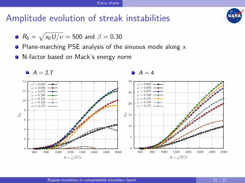
Extra charts

Amplitude evolution of streak instabilitiesR0 =

√x0U/ν = 500 and β = 0.30

Plane-marching PSE analysis of the sinuous mode along xN-factor based on Mack’s energy norm

A = 2.7

0

2

4

6

8

10

12

14

600 800 1000 1200 1400 1600 1800 2000

NE

R =√xU/ν

ω = 0.025ω = 0.050ω = 0.075ω = 0.100ω = 0.125ω = 0.150ω = 0.175

A = 4

0

5

10

15

20

25

30

600 800 1000 1200 1400 1600 1800 2000

NE

R =√xU/ν

ω = 0.025ω = 0.050ω = 0.075ω = 0.100ω = 0.125ω = 0.150ω = 0.175


Computational AeroSciences Branch NASA Langley Research …€¦ · Bypass transition in...

Documents

Transcript of Computational AeroSciences Branch NASA Langley Research …€¦ · Bypass transition in...