Computation1.pdf
18
MISSING DATA IN A POLYGON Surveying Engineering Department Ferris State University COMPUTING MISSING DATA USING THE GEOMETRIC APPROACH The conventional approach of solving the missing data problem is shown in figure 1. On the left is the traverse as it exists in the field. But, two data items are missing. Depending on the situation, a combination of two items given from s 1 , s 2 , α 1 , or α 2 are unknown. Then, one simply draws the sides of the traverse which are known. Then the unknown lines are grouped together. Thus, the traverse consists of an open traverse with line numbers 12, 14 and 15 drawn in a group. The coordinates of points A and C’ are computed by processing this open traverse. Then the distance and directions between A and C’ can be computed and the triangle composed of AB’C’ is computed using coordinate geometry. There are three basic forms in which the missing data problem can be formulated. An example from Hashimi [1988] is shown for each case. = Traverse Station = Distance of line = Line number = Azimuth of line BC 15 EA A EA S S 1 E S DE DE 14 D 2 11 1 12 13 S 2 C BC 11 S B S A E A 15 11 14 D' C' 12 13 B' Figure 1. Traverse showing missing elements. 1. Missing the distance and direction of the same line. This problem is very simple to solve. Determine the X and Y coordinates of each of the points in the traverse. This usually means starting at one known point and going both clockwise and counterclockwise until the unknown line is reached. Once the coordinates are found, inverse between them to find the distance and direction of the line. 6
-
Upload
abdelkhalek-bouanani -
Category
Documents
-
view
15 -
download
2
Transcript of Computation1.pdf

MISSING DATA IN A POLYGON
Surveying Engineering Department Ferris State University
COMPUTING MISSING DATA USING THE GEOMETRIC
APPROACH
The conventional approach of solving the missing data problem is shown in figure 1. On the left is the traverse as it exists in the field. But, two data items are missing. Depending on the situation, a combination of two items given from s1, s2, α1, or α2 are unknown. Then, one simply draws the sides of the traverse which are known. Then the unknown lines are grouped together. Thus, the traverse consists of an open traverse with line numbers 12, 14 and 15 drawn in a group. The coordinates of points A and C’ are computed by processing this open traverse. Then the distance and directions between A and C’ can be computed and the triangle composed of AB’C’ is computed using coordinate geometry. There are three basic forms in which the missing data problem can be formulated. An example from Hashimi [1988] is shown for each case.
= Traverse Station
= Distance of line
= Line number
= Azimuth of line
BC
15
EA
A
EAS
S 1
E S DE DE
14
D
2
11
1
12
13 S 2
C
BC
11
S
B
S
A
E
A
15
11
14 D'
C'
12
13
B'
Figure 1. Traverse showing missing elements. 1. Missing the distance and direction of the same line. This problem is very simple to
solve. Determine the X and Y coordinates of each of the points in the traverse. This usually means starting at one known point and going both clockwise and counterclockwise until the unknown line is reached. Once the coordinates are found, inverse between them to find the distance and direction of the line.
6
SURE 215 – Surveying Calculations Missing Data in a Polygon Page 2
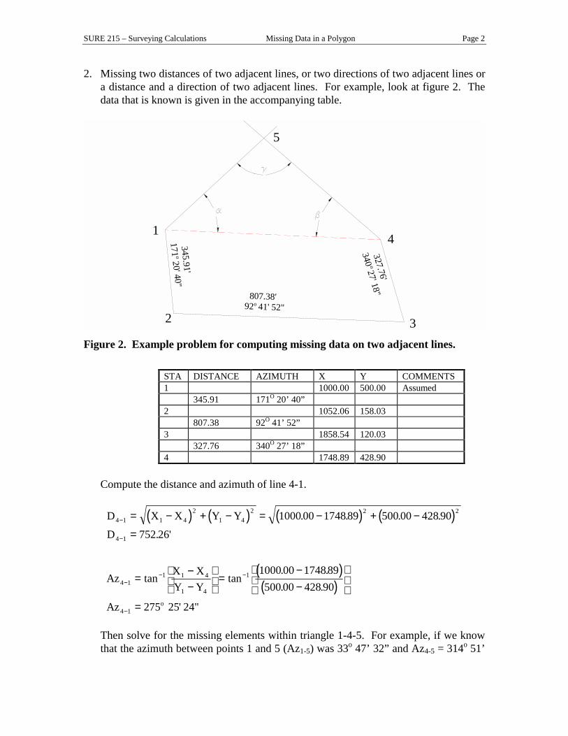
2. Missing two distances of two adjacent lines, or two directions of two adjacent lines or a distance and a direction of two adjacent lines. For example, look at figure 2. The data that is known is given in the accompanying table.
1
2 3
4
5
807.38'92 41' 52"
345.91'171 20' 40"
327.76'
340 27' 18"
o
o
o
Figure 2. Example problem for computing missing data on two adjacent lines.
STA DISTANCE AZIMUTH X Y COMMENTS 1 1000.00 500.00 Assumed 345.91 171O 20’ 40” 2 1052.06 158.03 807.38 92O 41’ 52” 3 1858.54 120.03 327.76 340O 27’ 18” 4 1748.89 428.90
Compute the distance and azimuth of line 4-1.
( ) ( ) ( ) ( )
( )( )
D X X Y Y
D
AzX XY Y
Az o
4 1 1 42
1 42 2 2
4 1
4 11 1 4
1 4
1
4 1
1000 00 1748 89 500 00 428 90
752 26
1000 00 1748 89500 00 428 90
275 25 24
−
−
−− −
−
= − + − = − + −
=
=−−
=
−−
=
. . . .
. '
tan tan. .. .
' "
Then solve for the missing elements within triangle 1-4-5. For example, if we know
that the azimuth between points 1 and 5 (Az1-5) was 33o 47’ 32” and Az4-5 = 314o 51’
SURE 215 – Surveying Calculations Missing Data in a Polygon Page 3
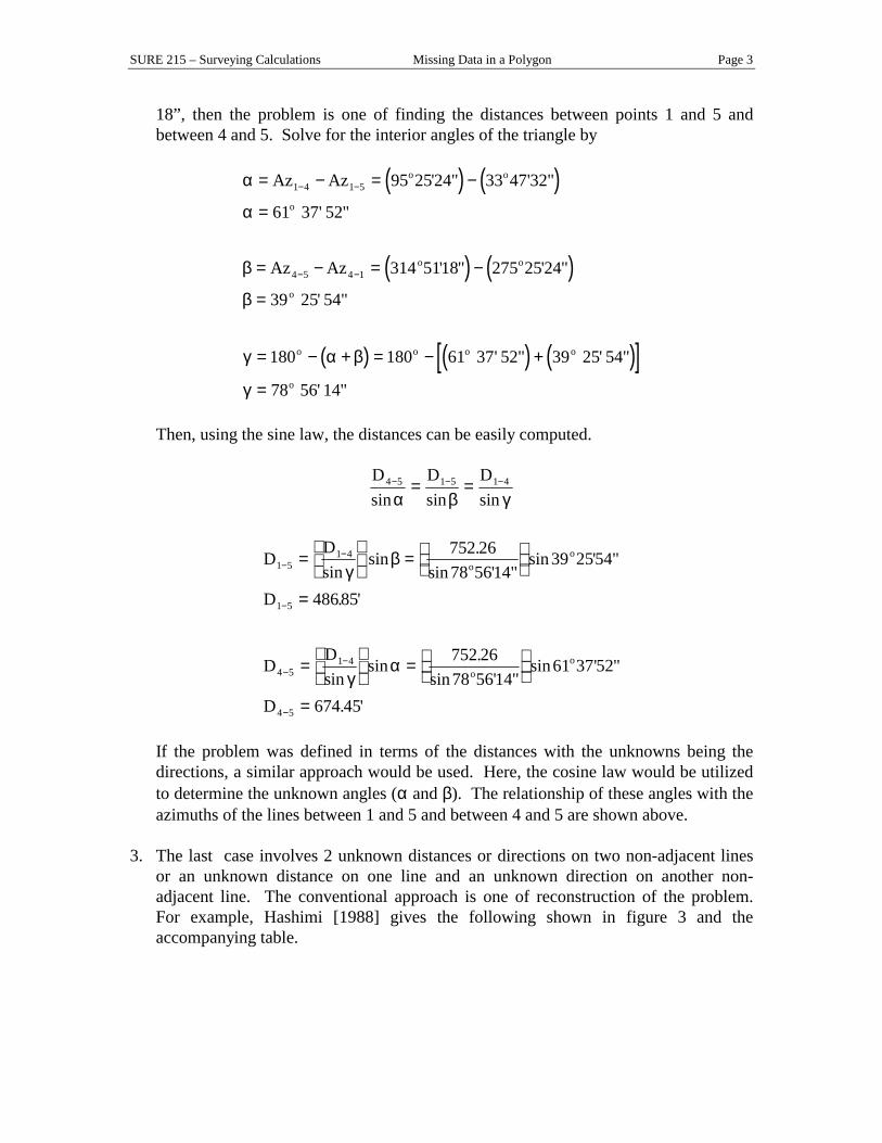
18”, then the problem is one of finding the distances between points 1 and 5 and between 4 and 5. Solve for the interior angles of the triangle by
( ) ( )
( ) ( )
( ) ( ) ( )[ ]
α
α
β
β
γ α β
γ
= − = −
=
= − = −
=
= − + = − +
=
− −
− −
Az Az
Az Az
o o
o
o o
o
o o o o
o
1 4 1 5
4 5 4 1
95 2524 33 47 32
61 37 52
314 5118 275 25 24
39 25 54
180 180 61 37 52 39 25 54
78 56 14
' " ' "
' "
' " ' "
' "
' " ' "
' "
Then, using the sine law, the distances can be easily computed.
D D D4 5 1 5 1 4− − −= =sin sin sinα β γ
DD
D
DD
D
oo
oo
1 51 4
1 5
4 51 4
4 5
752 2678 5614
39 2554
48685
752 2678 5614
61 37 52
674 45
−−
−
−−
−
=
=
=
=
=
=
sinsin .
sin ' "sin ' "
. '
sinsin .
sin ' "sin ' "
. '
γβ
γα
If the problem was defined in terms of the distances with the unknowns being the
directions, a similar approach would be used. Here, the cosine law would be utilized to determine the unknown angles (α and β). The relationship of these angles with the azimuths of the lines between 1 and 5 and between 4 and 5 are shown above.
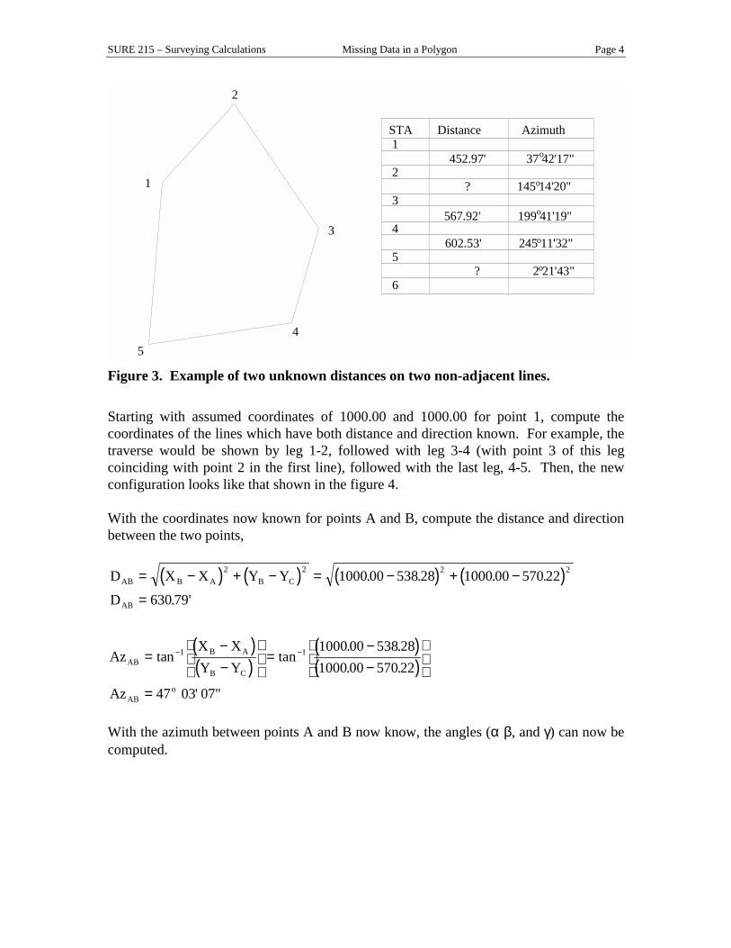
3. The last case involves 2 unknown distances or directions on two non-adjacent lines
or an unknown distance on one line and an unknown direction on another non-adjacent line. The conventional approach is one of reconstruction of the problem. For example, Hashimi [1988] gives the following shown in figure 3 and the accompanying table.
SURE 215 – Surveying Calculations Missing Data in a Polygon Page 4
1
2
3
45
STA Distance Azimuth 1
452.97' 37 42'17" 2
? 145 14'20" 3
567.92' 199 41'19" 4
602.53' 245 11'32" 5
? 2 21'43" 6
o
o
o
o
o
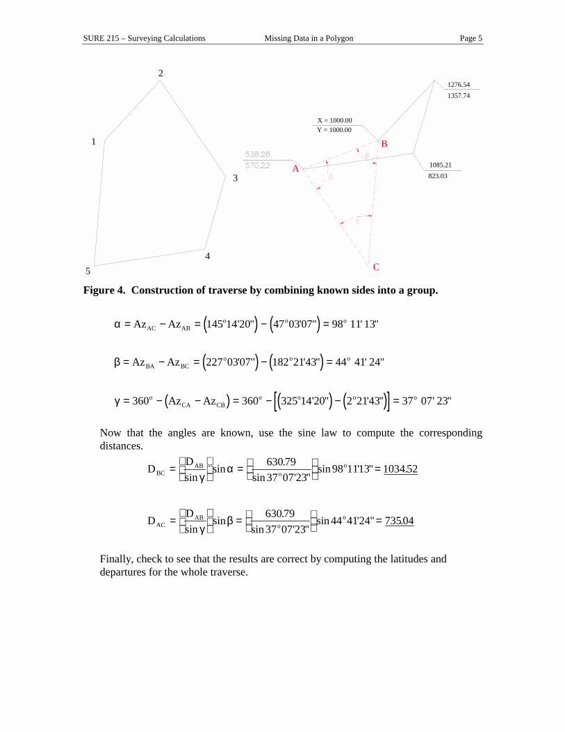
Figure 3. Example of two unknown distances on two non-adjacent lines. Starting with assumed coordinates of 1000.00 and 1000.00 for point 1, compute the coordinates of the lines which have both distance and direction known. For example, the traverse would be shown by leg 1-2, followed with leg 3-4 (with point 3 of this leg coinciding with point 2 in the first line), followed with the last leg, 4-5. Then, the new configuration looks like that shown in the figure 4. With the coordinates now known for points A and B, compute the distance and direction between the two points,
( ) ( ) ( ) ( )
( )( )
( )( )
D X X Y Y
D
AzX XY Y
Az
AB B A B C
AB
ABB A
B C
ABo
= − + − = − + −
=
=−−
=
−−
=
− −
2 2 2 2
1 1
1000 00 538 28 1000 00 570 22
630 79
1000 00 538 281000 00 570 22
47 03 07
. . . .
. '
tan tan. .. .
' "
With the azimuth between points A and B now know, the angles (α β, and γ) can now be computed.
SURE 215 – Surveying Calculations Missing Data in a Polygon Page 5
1
2
3
45
A
B
C
X = 1000.00Y = 1000.00
1276.541357.74
1085.21 823.03
Figure 4. Construction of traverse by combining known sides into a group.
( ) ( )
( ) ( )
( ) ( ) ( )[ ]
α
β
γ
= − = − =
= − = − =
= − − = − − =
Az Az
Az Az
Az Az
AC ABo o o
BA BCo o o
oCA CB
o o o o
145 14 20 47 03 07 98 11 13
227 0307 182 2143 44 41 24
360 360 325 14 20 2 2143 37 07 23
' " ' " ' "
' " ' " ' "
' " ' " ' "
Now that the angles are known, use the sine law to compute the corresponding
distances.
DD
DD
BCAB
oo
ACAB
oo
=
=
=
=
=
=
sinsin .
sin ' "sin ' " .
sinsin .
sin ' "sin ' " .
γα
γβ
630 7937 07 23
98 1113 1034 52
630 7937 07 23
44 4124 73504
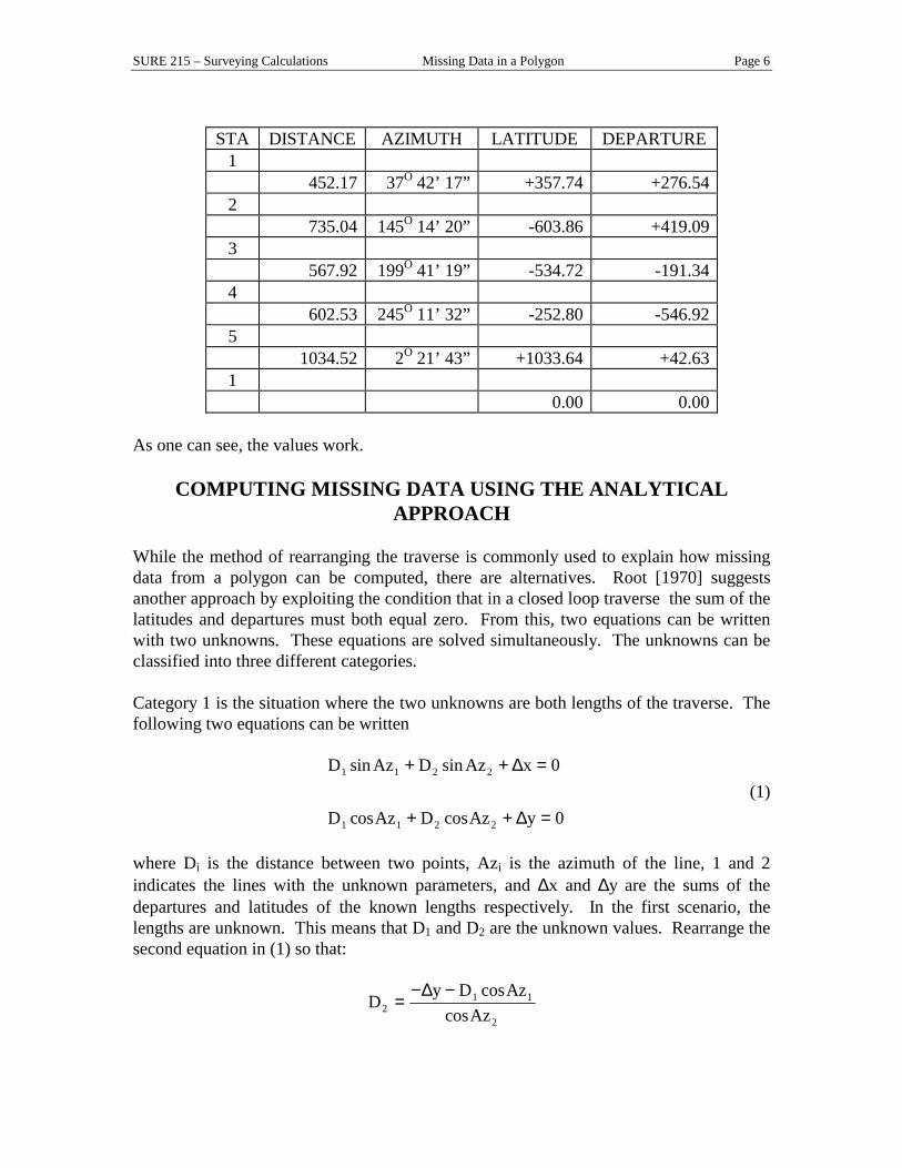
Finally, check to see that the results are correct by computing the latitudes and
departures for the whole traverse.
SURE 215 – Surveying Calculations Missing Data in a Polygon Page 6
STA DISTANCE AZIMUTH LATITUDE DEPARTURE
1 452.17 37O 42’ 17” +357.74 +276.54 2 735.04 145O 14’ 20” -603.86 +419.09 3 567.92 199O 41’ 19” -534.72 -191.34 4 602.53 245O 11’ 32” -252.80 -546.92 5 1034.52 2O 21’ 43” +1033.64 +42.63 1
0.00 0.00 As one can see, the values work.
COMPUTING MISSING DATA USING THE ANALYTICAL APPROACH
While the method of rearranging the traverse is commonly used to explain how missing data from a polygon can be computed, there are alternatives. Root [1970] suggests another approach by exploiting the condition that in a closed loop traverse the sum of the latitudes and departures must both equal zero. From this, two equations can be written with two unknowns. These equations are solved simultaneously. The unknowns can be classified into three different categories. Category 1 is the situation where the two unknowns are both lengths of the traverse. The following two equations can be written
D Az D Az x
D Az D Az y
1 1 2 2
1 1 2 2
0
0
sin sin
cos cos
+ + =
+ + =
∆
∆ (1)
where Di is the distance between two points, Azi is the azimuth of the line, 1 and 2 indicates the lines with the unknown parameters, and ∆x and ∆y are the sums of the departures and latitudes of the known lengths respectively. In the first scenario, the lengths are unknown. This means that D1 and D2 are the unknown values. Rearrange the second equation in (1) so that:
Dy D Az
Az21 1
2
=− −∆ cos
cos
SURE 215 – Surveying Calculations Missing Data in a Polygon Page 7
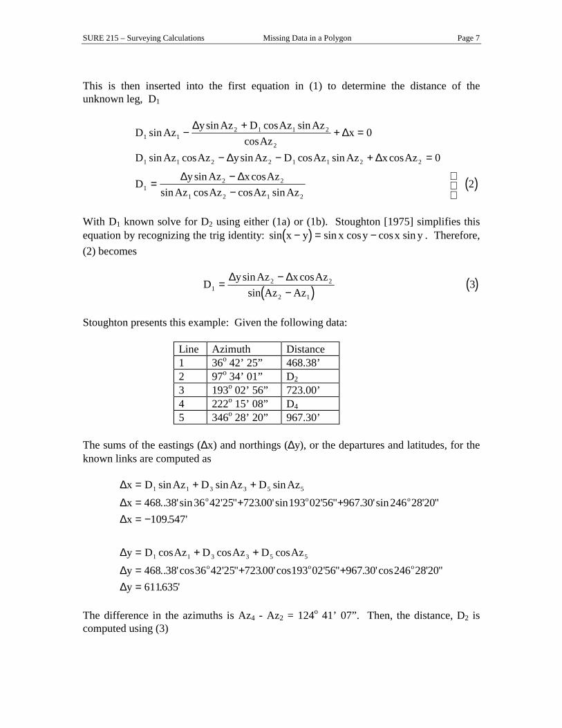
This is then inserted into the first equation in (1) to determine the distance of the unknown leg, D1
( )
D Azy Az D Az Az
Azx
D Az Az y Az D Az Az x Az
Dy Az x Az
Az Az Az Az
1 12 1 1 2
2
1 1 2 2 1 1 2 2
12 2
1 2 1 2
0
0
2
sinsin cos sin
cossin cos sin cos sin cos
sin cossin cos cos sin
−+
+ =
− − + =
=−−
∆∆
∆ ∆
∆ ∆
With D1 known solve for D2 using either (1a) or (1b). Stoughton [1975] simplifies this equation by recognizing the trig identity: ( )sin sin cos cos sinx y x y x y− = − . Therefore, (2) becomes
( ) ( )Dy Az x Az
Az Az12 2
2 1
3=−
−∆ ∆sin cos
sin
Stoughton presents this example: Given the following data:
Line Azimuth Distance 1 36o 42’ 25” 468.38’ 2 97o 34’ 01” D2 3 193o 02’ 56” 723.00’ 4 222o 15’ 08” D4 5 346o 28’ 20” 967.30’
The sums of the eastings (∆x) and northings (∆y), or the departures and latitudes, for the known links are computed as
∆
∆∆
∆
∆∆
x D Az D Az D Azxx
y D Az D Az D Azyy
o o o
o o o
= + +
= + += −
= + +
= + +=
1 1 3 3 5 5
1 1 3 3 5 5
468 38 36 42 25 72300 193 02 56 967 30 246 28 20109 547
468 38 36 42 25 723 00 193 02 56 967 30 246 28 20611635
sin sin sin.. ' sin ' " . ' sin ' " . ' sin ' "
. '
cos cos cos.. 'cos ' " . 'cos ' " . 'cos ' ". '
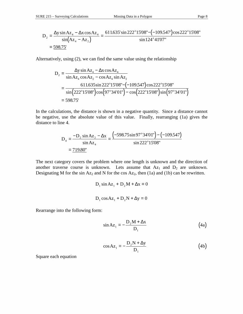
The difference in the azimuths is Az4 - Az2 = 124o 41’ 07”. Then, the distance, D2 is computed using (3)
SURE 215 – Surveying Calculations Missing Data in a Polygon Page 8
( )( )
Dy Az x Az
Az Az
o o
o24 4
4 2
611635 222 1508 109 547 222 1508124 4107
598 75
=−
−=
− −
=
∆ ∆sin cossin
. ' sin ' " . ' cos ' "sin ' "
. '
Alternatively, using (2), we can find the same value using the relationship
( )( ) ( ) ( ) ( )
D y Az x AzAz Az Az Az
o o
o o o o
24 4
4 2 4 2
611635 222 15 08 109 547 222 15 08222 15 08 97 34 01 222 15 08 97 34 01
598 75
= −−
=− −
−
=
∆ ∆sin cossin cos cos sin
. sin ' " . cos ' "sin ' " cos ' " cos ' " sin ' "
. '
In the calculations, the distance is shown in a negative quantity. Since a distance cannot be negative, use the absolute value of this value. Finally, rearranging (1a) gives the distance to line 4.
( ) ( )D
D Az xAz
o
o42 2
4
598 75 97 34 01 109 547
222 1508719 80
=− −
=− − −
=
sinsin
. sin ' " .
sin ' ". "
∆
The next category covers the problem where one length is unknown and the direction of another traverse course is unknown. Lets assume that Az1 and D2 are unknown. Designating M for the sin Az2 and N for the cos Az2, then (1a) and (1b) can be rewritten.
D Az D M x
D Az D N y
1 1 2
1 1 2
0
0
sin
cos
+ + =
+ + =
∆
∆
Rearrange into the following form:
( )
( )
sin
cos
AzD M x
Da
AzD N y
Db
12
1
12
1
4
4
= −+
= −+
∆
∆
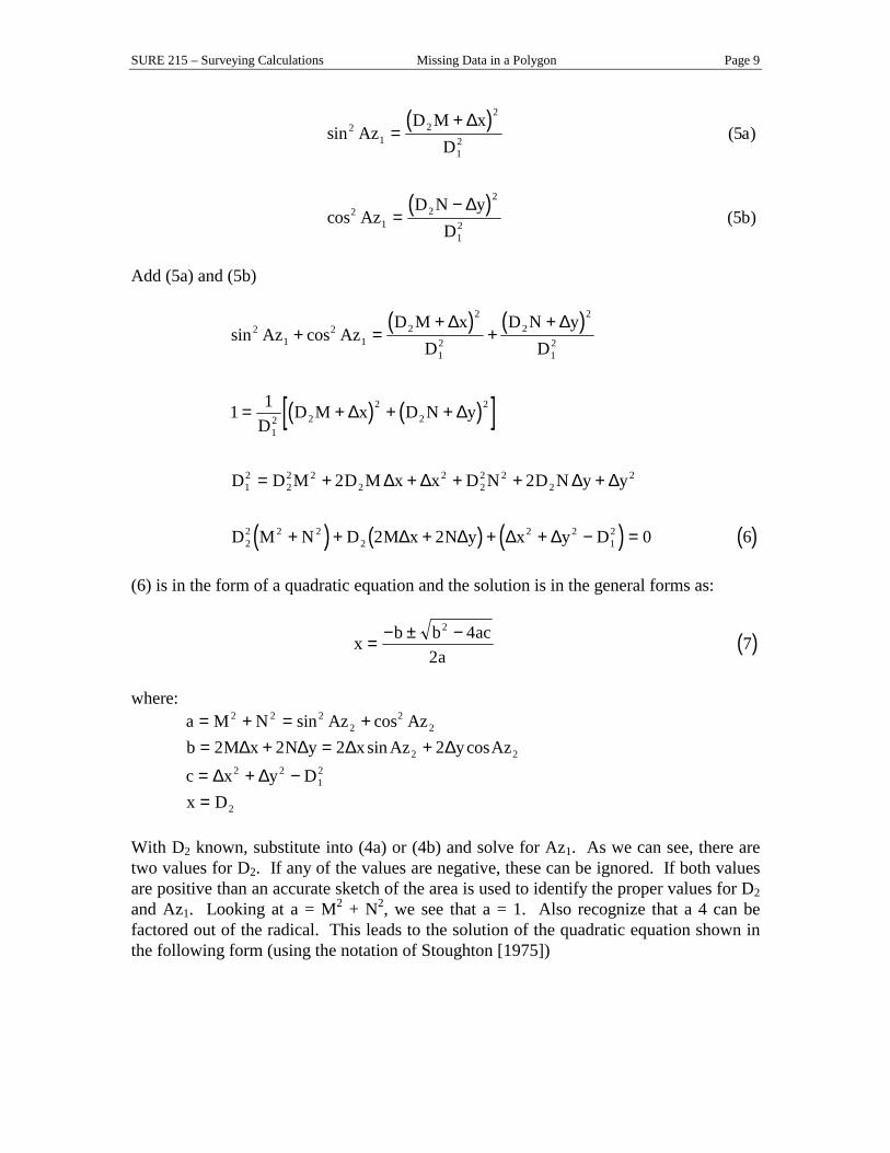
Square each equation
SURE 215 – Surveying Calculations Missing Data in a Polygon Page 9
( )
( )
sin (5 )
cos (5 )
21
22
12
21
22
12
AzD M x
Da
AzD N y
Db
=+
=−
∆
∆
Add (5a) and (5b)
( ) ( )
( ) ( )[ ]
( ) ( ) ( ) ( )
sin cos21
21
22
12
22
12
12 2
22
2
12
22 2
22
22 2
22
22 2 2
22 2
12
1 1
2 2
2 2 0 6
Az AzD M x
DD N y
D
DD M x D N y
D D M D M x x D N D N y y
D M N D M x N y x y D
+ =+
++
= + + +
= + + + + +
+ + + + + − =
∆ ∆
∆ ∆
∆ ∆ ∆ ∆
∆ ∆ ∆ ∆
(6) is in the form of a quadratic equation and the solution is in the general forms as:
( )x b b aca
= − ± −2 42
7
where:
a M N Az Azb M x N y x Az y Azc x y Dx D
= + = += + = +
= + −=
2 2 22
22
2 22 2
12
2
2 2 2 2sin cos
sin cos∆ ∆ ∆ ∆
∆ ∆
With D2 known, substitute into (4a) or (4b) and solve for Az1. As we can see, there are two values for D2. If any of the values are negative, these can be ignored. If both values are positive than an accurate sketch of the area is used to identify the proper values for D2 and Az1. Looking at a = M2 + N2, we see that a = 1. Also recognize that a 4 can be factored out of the radical. This leads to the solution of the quadratic equation shown in the following form (using the notation of Stoughton [1975])

SURE 215 – Surveying Calculations Missing Data in a Polygon Page 10
D V V U
V V U
1
2
2
2 4 42
= − ± −
= − ± −
(8)
where:
U x y D andV xM yN
= + −= +
∆ ∆∆ ∆
2 222 ,
Example, from Stoughton [1975]. Given the following traverse data, compute D2 and Az4.
Line Azimuth Distance 1 36o 42’ 25” 468.38’ 2 97o 34’ 01” D2 3 193o 02’ 56” 723.00’ 4 Az4 719.80 5 346o 28’ 20” 967.30’
The solution is as follows.
( ) ( ) ( )( ) ( )
U x y D
V x Az y Az o o
= + − = − + − = −
= + = − + = −
∆ ∆
∆ ∆
2 242 2 2 2
2 2
109 547 611635 719 80 132 0141216
109 547 97 34 01 611635 97 34 01 189 13588
. . . , .
sin cos . sin ' " . cos ' " . Substitute these values into (8) yields:
( ) ( ) ( )D V V U
or2
2 218913588 18913588 132 0141216
598 75 220 48
= − ± − = − − ± − − −
= −
. . , .
. ' . '
The last value is not possible therefore the solution is D2 = 598.75’. Substitute this value into (4a) or (4b) to solve for the azimuth of line 4.
( )Az
D M xD
o
o
41 2
4
1 598 75 97 34 01 109 547719 80
42 15 08
=+
=
− − −
= −
− −sin sin. sin ' " .
.
' "
∆
This result shows that the azimuth is in either the northwest or southwest quadrant. A good drawing of the traverse would show that it needs to be in the southwest quadrant therefore the azimuth is 222o 15’ 08”. This should be verified by computing the latitudes and departures for the traverse. For example, the azimuth of 222o 15’ 08” results in a closed traverse as shown in the accompanying spreadsheet.
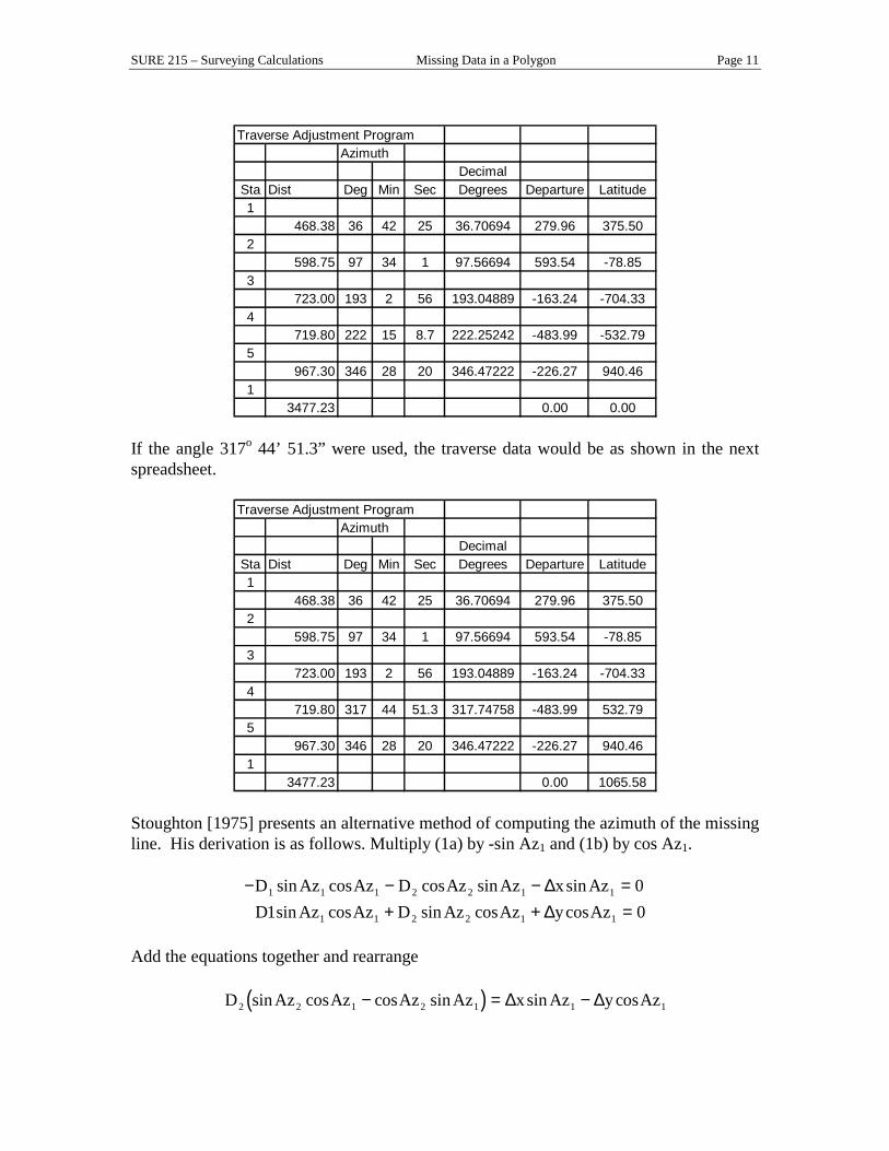
SURE 215 – Surveying Calculations Missing Data in a Polygon Page 11
Traverse Adjustment Program
Azimuth Decimal
Sta Dist Deg Min Sec Degrees Departure Latitude1
468.38 36 42 25 36.70694 279.96 375.502
598.75 97 34 1 97.56694 593.54 -78.853
723.00 193 2 56 193.04889 -163.24 -704.334
719.80 222 15 8.7 222.25242 -483.99 -532.795
967.30 346 28 20 346.47222 -226.27 940.461
3477.23 0.00 0.00 If the angle 317o 44’ 51.3” were used, the traverse data would be as shown in the next spreadsheet.
Traverse Adjustment Program Azimuth Decimal
Sta Dist Deg Min Sec Degrees Departure Latitude1
468.38 36 42 25 36.70694 279.96 375.502
598.75 97 34 1 97.56694 593.54 -78.853
723.00 193 2 56 193.04889 -163.24 -704.334
719.80 317 44 51.3 317.74758 -483.99 532.795
967.30 346 28 20 346.47222 -226.27 940.461
3477.23 0.00 1065.58 Stoughton [1975] presents an alternative method of computing the azimuth of the missing line. His derivation is as follows. Multiply (1a) by -sin Az1 and (1b) by cos Az1.
− − − =+ + =
D Az Az D Az Az x AzD Az Az D Az Az y Az
1 1 1 2 2 1 1
1 1 2 2 1 1
01 0
sin cos cos sin sinsin cos sin cos cos
∆∆
Add the equations together and rearrange
( )D Az Az Az Az x Az y Az2 2 1 2 1 1 1sin cos cos sin sin cos− = −∆ ∆
SURE 215 – Surveying Calculations Missing Data in a Polygon Page 12
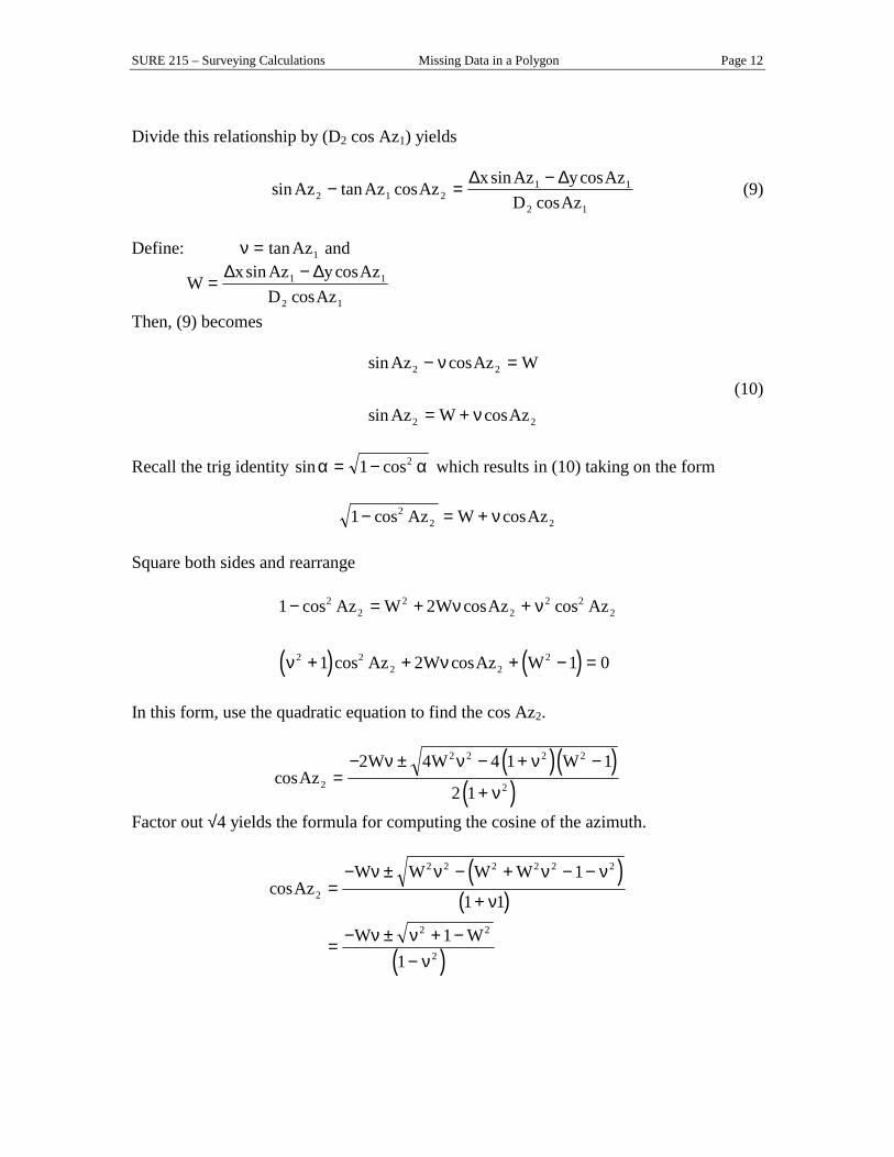
Divide this relationship by (D2 cos Az1) yields
sin tan cossin cos
cosAz Az Az
x Az y AzD Az2 1 2
1 1
2 1
− =−∆ ∆
(9)
Define: ν = tanAz1 and
Wx Az y Az
D Az=
−∆ ∆sin coscos1 1
2 1
Then, (9) becomes
sin cos
sin cos
Az Az W
Az W Az
2 2
2 2
− =
= +
ν
ν (10)
Recall the trig identity sin cosα α= −1 2 which results in (10) taking on the form
1 22 2− = +cos cosAz W Azν
Square both sides and rearrange
( ) ( )
1 2
1 2 1 0
22
22
2 22
2 22 2
2
− = + +
+ + + − =
cos cos cos
cos cos
Az W W Az Az
Az W Az W
ν ν
ν ν
In this form, use the quadratic equation to find the cos Az2.
( )( )( )cosAz
W W W2
2 2 2 2
2
2 4 4 1 1
2 1=
− ± − + −
+
ν ν ν
ν
Factor out √4 yields the formula for computing the cosine of the azimuth.
( )( )
( )
cosAzW W W W
W W
2
2 2 2 2 2 2
2 2
2
1
1 1
11
=− ± − + − −
+
= − ± + −−
ν ν ν ν
ν
ν νν
SURE 215 – Surveying Calculations Missing Data in a Polygon Page 13
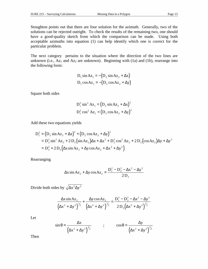
Stoughton points out that there are four solution for the azimuth. Generally, two of the solutions can be rejected outright. To check the results of the remaining two, one should have a good-quality sketch from which the comparison can be made. Using both acceptable azimuths into equation (1) can help identify which one is correct for the particular problem. The next category pertains to the situation where the direction of the two lines are unknown (i.e., Az1 and Az2 are unknown). Beginning with (1a) and (1b), rearrange into the following form:
( )( )
D Az D Az x
D Az D Az y1 1 2 2
1 1 2 2
sin sin
cos cos
= − +
= − +
∆
∆
Square both sides
( )( )
D Az D Az x
D Az D Az y12 2
1 2 22
12 2
1 2 22
sin sin
cos cos
= +
= +
∆
∆
Add these two equations yields
( ) ( )( ) ( )
( )
D D Az x D Az y
D Az D Az x x D Az D Az y y
D D x Az y Az x y
12
2 22
2 22
22 2
2 2 22
22 2
2 2 22
22
2 2 22 2
2 2
2
= + + +
= + + + + +
= + + + +
sin cos
sin sin cos cos
sin cos
∆ ∆
∆ ∆ ∆ ∆
∆ ∆ ∆ ∆
Rearranging
∆ ∆∆ ∆
x Az y AzD D x y
Dsin cos2 2
12
22 2 2
22+ =
− − −
Divide both sides by ∆ ∆x y2 2
( ) ( ) ( )∆
∆ ∆
∆
∆ ∆
∆ ∆
∆ ∆
x Az
x y
y Az
x y
D D x y
D x y
sin cos2
2 21
2
2
2 21
2
12
22 2 2
22 2
122+
++
=− − −
+
Let
( ) ( )sin ; cosθ θ=
+=
+
∆
∆ ∆
∆
∆ ∆
x
x y
y
x y2 21
2 2 21
2
Then
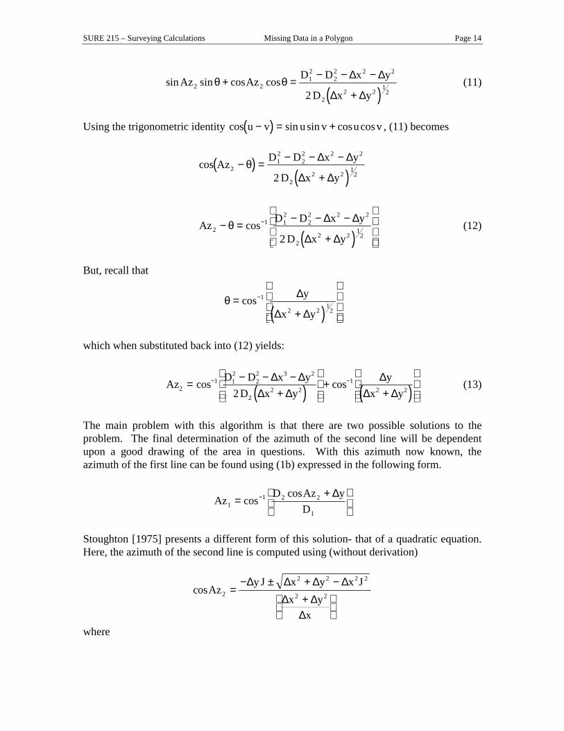
SURE 215 – Surveying Calculations Missing Data in a Polygon Page 14
( )sin sin cos cosAz Az
D D x y
D x y2 2
12
22 2 2
22 2
122
θ θ+ =− − −
+
∆ ∆
∆ ∆ (11)
Using the trigonometric identity ( )cos sin sin cos cosu v u v u v− = + , (11) becomes
( )( )
cos AzD D x y
D x y2
12
22 2 2
22 2
122
− =− − −
+θ
∆ ∆
∆ ∆
( )Az
D D x y
D x y2
1 12
22 2 2
22 2
122
− =− − −
+
−θ cos∆ ∆
∆ ∆ (12)
But, recall that
( )θ =
+
−cos 1
2 21
2
∆
∆ ∆
y
x y
which when substituted back into (12) yields:
( ) ( )Az D D x yD x y
yx y2
1 12
22 3 2
22 2
12 22
= − − −+
++
− −cos cos∆ ∆∆ ∆
∆∆ ∆
(13)
The main problem with this algorithm is that there are two possible solutions to the problem. The final determination of the azimuth of the second line will be dependent upon a good drawing of the area in questions. With this azimuth now known, the azimuth of the first line can be found using (1b) expressed in the following form.
AzD Az y
D11 2 2
1
=+
−coscos ∆
Stoughton [1975] presents a different form of this solution- that of a quadratic equation. Here, the azimuth of the second line is computed using (without derivation)
cosAzy J x y x J
x yx
2
2 2 2 2
2 2=
− ± + −+
∆ ∆ ∆ ∆∆ ∆
∆
where
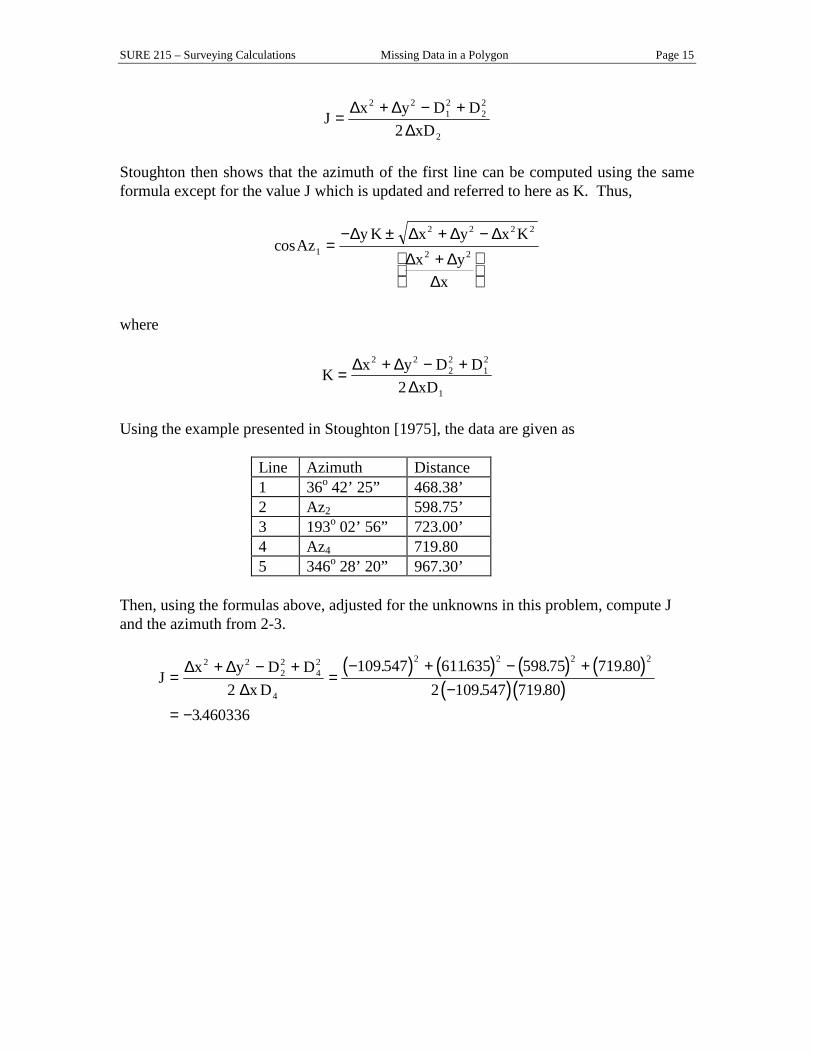
SURE 215 – Surveying Calculations Missing Data in a Polygon Page 15
Jx y D D
xD=
+ − +∆ ∆∆
2 212
22
22
Stoughton then shows that the azimuth of the first line can be computed using the same formula except for the value J which is updated and referred to here as K. Thus,
cosAzy K x y x K
x yx
1
2 2 2 2
2 2=
− ± + −+
∆ ∆ ∆ ∆∆ ∆
∆
where
Kx y D D
xD=
+ − +∆ ∆∆
2 222
12
12
Using the example presented in Stoughton [1975], the data are given as
Line Azimuth Distance 1 36o 42’ 25” 468.38’ 2 Az2 598.75’ 3 193o 02’ 56” 723.00’ 4 Az4 719.80 5 346o 28’ 20” 967.30’
Then, using the formulas above, adjusted for the unknowns in this problem, compute J and the azimuth from 2-3.
( ) ( ) ( ) ( )( )( )J
x y D Dx D
=+ − +
=− + − +
−= −
∆ ∆∆
2 222
42
4
2 2 2 2
2109 547 611635 598 75 719 80
2 109 547 719 803 460336
. . . .. .
.
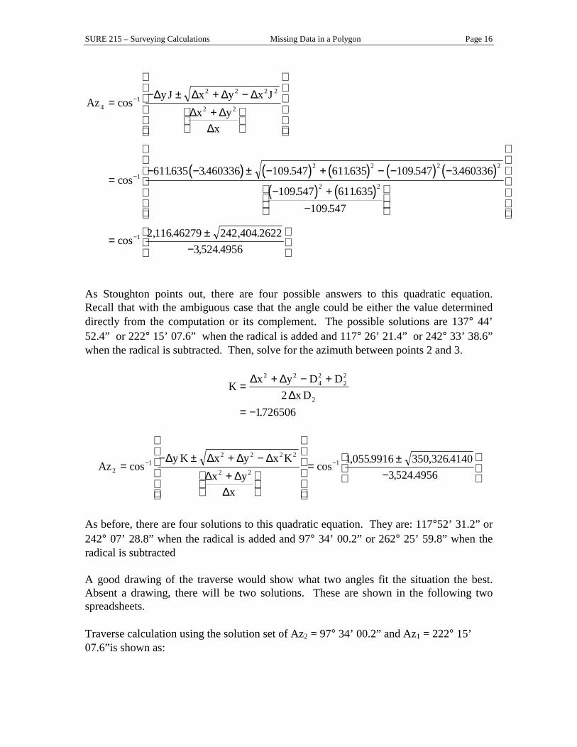
SURE 215 – Surveying Calculations Missing Data in a Polygon Page 16
( ) ( ) ( ) ( ) ( )( ) ( )
Azy J x y x J
x yx
41
2 2 2 2
2 2
12 2 2 2
2 2
1
611635 3 460336 109 547 611635 109 547 3460336
109 547 611635109 547
2 116 46279 242 404 26223 524 4956
=− ± + −
+
=− − ± − + − − −
− +−
= ±−
−
−
−
cos
cos. . . . . .
. ..
cos , . , ., .
∆ ∆ ∆ ∆∆ ∆
∆
As Stoughton points out, there are four possible answers to this quadratic equation. Recall that with the ambiguous case that the angle could be either the value determined directly from the computation or its complement. The possible solutions are 137° 44’ 52.4” or 222° 15’ 07.6” when the radical is added and 117° 26’ 21.4” or 242° 33’ 38.6” when the radical is subtracted. Then, solve for the azimuth between points 2 and 3.
Kx y D D
x D=
+ − +
= −
∆ ∆∆
2 242
22
221726506.
Azy K x y x K
x yx
21
2 2 2 2
2 21 1 055 9916 350 326 4140
3 524 4956=
− ± + −+
=±
−
− −cos cos
, . , ., .
∆ ∆ ∆ ∆∆ ∆
∆
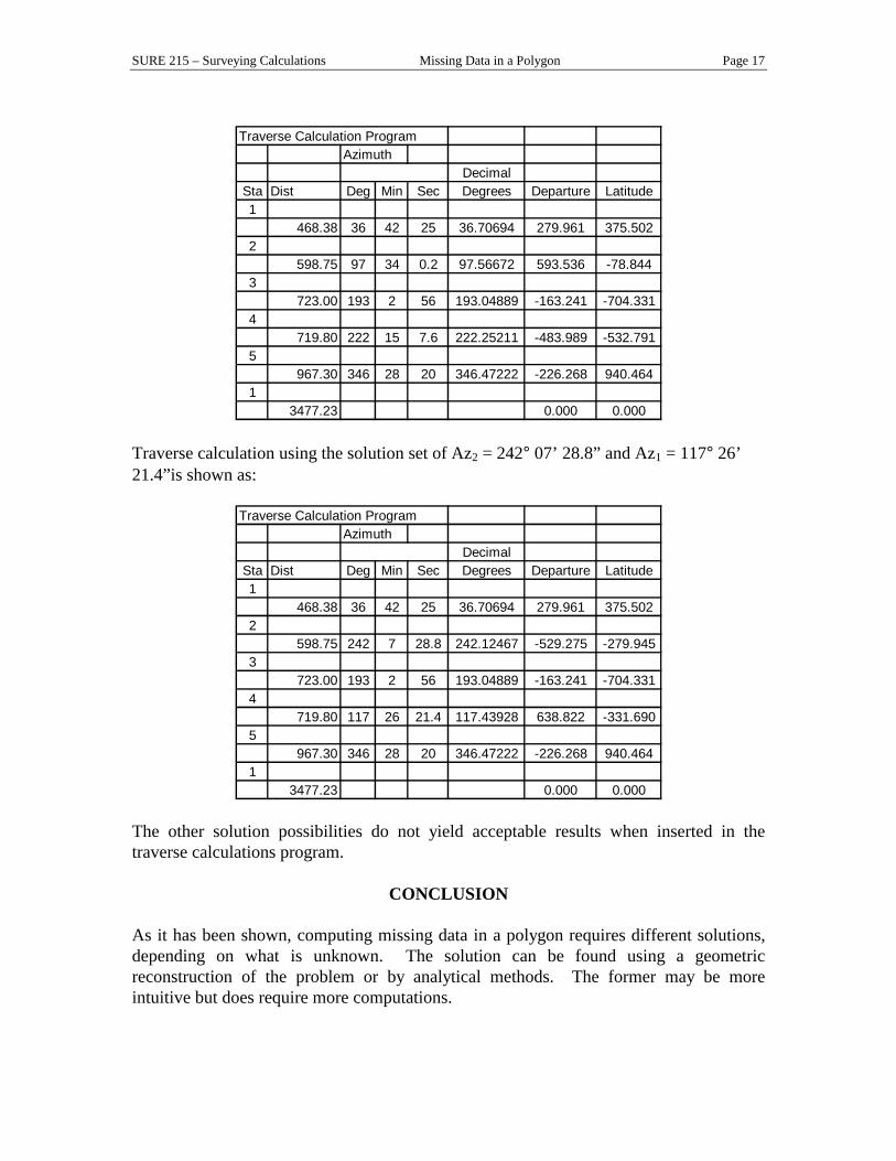
As before, there are four solutions to this quadratic equation. They are: 117°52’ 31.2” or 242° 07’ 28.8” when the radical is added and 97° 34’ 00.2” or 262° 25’ 59.8” when the radical is subtracted A good drawing of the traverse would show what two angles fit the situation the best. Absent a drawing, there will be two solutions. These are shown in the following two spreadsheets. Traverse calculation using the solution set of Az2 = 97° 34’ 00.2” and Az1 = 222° 15’ 07.6”is shown as:
SURE 215 – Surveying Calculations Missing Data in a Polygon Page 17
Traverse Calculation Program
Azimuth Decimal
Sta Dist Deg Min Sec Degrees Departure Latitude1
468.38 36 42 25 36.70694 279.961 375.5022
598.75 97 34 0.2 97.56672 593.536 -78.8443
723.00 193 2 56 193.04889 -163.241 -704.3314
719.80 222 15 7.6 222.25211 -483.989 -532.7915
967.30 346 28 20 346.47222 -226.268 940.4641
3477.23 0.000 0.000 Traverse calculation using the solution set of Az2 = 242° 07’ 28.8” and Az1 = 117° 26’ 21.4”is shown as:
Traverse Calculation ProgramAzimuth Decimal
Sta Dist Deg Min Sec Degrees Departure Latitude1
468.38 36 42 25 36.70694 279.961 375.5022
598.75 242 7 28.8 242.12467 -529.275 -279.9453
723.00 193 2 56 193.04889 -163.241 -704.3314
719.80 117 26 21.4 117.43928 638.822 -331.6905
967.30 346 28 20 346.47222 -226.268 940.4641
3477.23 0.000 0.000 The other solution possibilities do not yield acceptable results when inserted in the traverse calculations program.
CONCLUSION As it has been shown, computing missing data in a polygon requires different solutions, depending on what is unknown. The solution can be found using a geometric reconstruction of the problem or by analytical methods. The former may be more intuitive but does require more computations.

SURE 215 – Surveying Calculations Missing Data in a Polygon Page 18
The problem may have no unique solution. This occurs when the directions of two sides are unknown. In such a situation, a good sketch of the field conditions will be required to resolve this ambiguity.
REFERENCES Hashimi, S., 1988. “SUR 221 - Surveying Calculations Lecture Notes”, Ferris State University, 90p. Root, J.A., 1970. “Computations for Missing Elements of Closed Traverses”, Surveying and Mapping, XXX(1):91-93. Stoughton, H.W., 1975. “Computing Missing Elements of a Polygon”, Surveying and Mapping, XXXV(3):217-222.