Compression Moulding of SMC - DiVA portal999288/... · 2016-09-30 · LICENTIATE THESIS Department...

LICENTIATE T H E S I S

Department of Applied Physics and Mechanical Engineering

Division of Fluid Mechanics

Compression Moulding of SMCExperiments and Simulation

N. E. Jimmy Olsson

ISSN: 1402-1757 ISBN 978-91-7439-184-8

Luleå University of Technology 2010

ISSN: 1402-1757 ISBN 978-91-7439-XXX-X Se i listan och fyll i siffror där kryssen är

Compression Moulding of SMC

Experiments and Simulation

N. E. Jimmy Olsson

Luleå University of TechnologyDepartment of Applied Physics and Mechanical Engineering

Division of Fluid Mechanics

Printed by Universitetstryckeriet, Luleå 2010

ISSN: 1402-1757 ISBN 978-91-7439-184-8

Luleå 2010

www.ltu.se

Abstract

Due to excellent properties and relatively low material and manufacturing costs, the use of fibre reinforced polymer composites have increased during the last decades. One method that is suitable for large scale productions of e.g. lightweight vehicle components is compression moulding of sheet moulding compound (SMC). Although the technique has been considerably improved since it first was introduced, some further improvements need to be done. The main reason why it has not come in wider use in the vehicle industry is unsatisfactory conditions of the surface finish of parts manufactured due to voids. In this work, experiments and numerical simulations has been performed in order to increase the knowledge of the flow behaviour during the compression moulding process and how the flow affect the quality of the finished product. A process parameter experiment of the compression moulding phase, carried out with a design of experiment approach, was performed in order to investigate the effect of vacuum assistance, mould temperature and ram velocity on the void transport and flow behaviour for SMC. The relative amount of voids has been quantified with a high voltage insulation test and the flow behaviour has been quantified with image analysis of samples moulded with coloured SMC. In conclusion, the setting of high vacuum, low ram velocity and low mould temperature creates a homogeneous flow and minimises the amount of voids. In order to further increase the understanding of void removal during compression moulding, a model experiment was performed where a non-Newtonian fluid (grease) with added bubbles was compressed between two plates whereas the motion of the bubbles were tracked and evaluated using Particle Image Velocimetry. The bubble motion was furthermore analytically modelled and coupled to the experimental results. The experiments reveal an increase in bubble speed compared to the surrounding grease during the compression of the plates. During the latter stage of the compression, the particles change form from initially being approximately spherical, to have the characteristic form of a falling raindrop. The change in form coincides with the increase in speed of the bubble. The developed analytical model supports the shown development in the experiments. A full general solution comprising an arbitrary value of the Power Law exponent, for the velocity fraction coefficient representing the relative bubble speed, is however not covered at the present stage. Finally, the commercial software Ansys CFX were used to perform computational fluid dynamics (CFD) modelling of the flow during compression moulding with a two different multiphase models. The first model treats the flow of SMC as purely extensional and dependent on temperature, fibre volume fraction and strain rate. While the other one sees the flow as mainly extensional but also with thin shear layers near the surfaces of the moulding tool. Where the viscosity, in addition to temperature, fibre volume fraction and strain rate, also is dependant on shear strain rate. Of the two models, the latter seems to be more robust in modelling the pressure during moulding.

PREFACE

This thesis was produced at the division of fluid mechanics at Luleå University of Technology, Sweden, as a part of the FYS-project which was financially supported by VINNOVA and is therefore gratefully acknowledged. Compression moulding experiments have been performed at Swerea SICOMP AB, Piteå, Sweden.

I have many to thank who have supported me in different ways during this project for which I am grateful, to mention everyone would be a too long list. However, there are some people that I especially would like to thank.

I would like to thank my main supervisor Professor Staffan Lundström, first for giving me the opportunity to participate in this project which have been very interesting and instructive for me, and also for his patience and guidance during the project.

The staff at Swerea SICOMP AB who have helped out with experiments and especially Kurt Olofsson who have been a co-supervisor for me and contributed with a lot of expertise in various questions.

All the co-workers at the division for making my time here pleasant, and a special thank to those who have supported me during the CFD phase, you know who you are. And of course a special thank to the PIV-expert Torbjörn Green who gave very helpful consulting during my PIV-experiment.

Allan Holmgren, the divisions own inventor who built the experimental setup for the squeeze flow visualisation.

Jerker Åberg, who had very helpful comments about CFD.

All the participants in the FYS-project, a lot of interesting discussions have been taking place.

The printing firm of the University for their charitable approach of my late submission…

I would like to thank my beloved Emma and our son Melvin for your encouraging help, especially the last few weeks!

PUBLICATIONS

A. Olsson, N.E.J., T.S. Lundstrom, and K. Olofsson, Design of experiment study of compression moulding of SMC. Plastics Rubber and Composites, 2009. 38(9-10): p. 426-431.

B. Westerberg, L.G., N.E.J. Olsson, and T.S. Lundstöm. Transport of bubbles during compression in a non-Newtonian fluid. in Proceedings of ITP2009 : Interdisciplinary Transport Phenomena VI: Fluid, Thermal, Biological, Materials and Space Sciences. 2009. Volterra, Italy.

C. Olsson, N.E.J., T.S. Lundstrom, and K. Olofsson, Compression moulding of SMC: Modelling with CFD and validation. Manuscript

Paper A

Pub

lishe

d by

Man

ey P

ublis

hing

(c)

IOM

Com

mun

icat

ions

Ltd

Design of experiment study of compressionmoulding of SMC

N. E. J. Olsson*1, T. S. Lundstrom1 and K. Olofsson2

The effect of vacuum assistance, mould temperature and ram velocity on the void transport and

flow behaviour for sheet moulding compound (SMC) have been investigated with a design of

experiment approach of the compression moulding phase. The relative amount of voids has been

quantified with a high voltage insulation test and the flow behaviour has been quantified with

image analysis of samples moulded with coloured SMC. In conclusion, the setting of high

vacuum, low ram velocity and low mould temperature creates a homogeneous flow and minimises

the amount of voids.

Keywords: SMC, Compression moulding, Vacuum, Flow, Void transport

IntroductionOwing to excellent properties and relatively low materialand manufacturing costs, the use of fibre reinforcedpolymer composites have increased during the latestdecades. One of the cost effective manufacturingmethods suitable for large scale productions, in e.g.the vehicle industry, is compression moulding of sheetmoulding compound (SMC). This manufacturingmethod can be briefly explained as a process with twomajor steps, manufacturing and compression mouldingof SMC prepreg sheets. In the preparation step, a highconcentration (15–35 wt-%) of chopped fibre strands israndomly spread in the plane between two layers of apaste that generally consists of three mixed ingredients:thermosetting resins, filler and additives. For enhancedimpregnation, the sheets are then compounded. This isfollowed by a maturation phase, where the sheets arestored for some time whose length depends on composi-tion of the paste. During the storage, the prepreg ischemically thickened, making the sheets more workable,and the dramatic increase in viscosity that results alsoaids transport of fibres into extremities of the geome-tries1 during compression. In the compression stage, thesheets are cut into pieces and placed inside a heatedmoulding tool at which compression moulding isapplied. During compression moulding, SMC undergoa very complex process with a first lowering of theviscoelastic properties initiated by heat transfer from themoulding tool. This is followed by solidification whichoccurs when the molecules start to grow in size by across-linking process, and a viscoelastic solid is finallyformed through polymerisation.1

Although inventions such as low profile additives andvacuum assisted mouldings have improved the quality

for SMC products considerably since the technique wasintroduced in the 1950s, some further improvementsneed to be carried out. One issue that still concerns theindustry is voids in the material and at the surface. Voidslocated at the surface may cause defects such as pinholesand blowouts2 which require rework or rejection for alarge number of parts which inhibit the success for SMCin the vehicle industry where it is of great importance tohave a surface appearance of high quality. Moreover,internal voids are also undesirable, especially in the highvoltage industry since they decrease the electricalinsulation properties.3

During manufacturing, air may be entrapped in theprepreg manufacturing phase as voids in the paste andfurther by poor fibre impregnation.4 Moreover, voidsmay also originate from the compression mouldingphase, due to air between the sheets in stacks, airentrapments due to complex flow and also boiling ofstyrene.4,5 Different methods have been developed toreduce the amount of voids in the prepreg sheets, inorder to oblique reduce the amount of voids inmanufactured products. However, results by Yamadaet al.6 show that the void content in prepregs has to bevery high to give an increased number of surface voids.This behaviour has also been confirmed by an initialexperiment, carried out by Nilsson at Swerea SICOMPAB, where the effect of a vacuum treatment method forprepregs (Fig. 1) was investigated.7 The experimentrevealed that the amount of voids in the prepregs hadno significant effect on the amount of voids after com-pression moulding even though this method decreasedthe initial void content in the prepreg to approximatelyone-third of the void content for the regular industriallymanufactured prepreg. Hence, it is important to gainknowledge of the flow behaviour during compressionmoulding and thereby diminish the amount of voids inSMC products and also to maintain flow control inorder to achieve in-plane isotropic mechanical proper-ties since the fibres align in the flow direction.8,9

Owing to the anisotropic non-Newtonian behaviourof SMC,10–12 it is difficult to establish a fully accurate

1Division of Fluid Mechanics, Lulea University of Technology, SE-971 87Lulea, Sweden2Swerea SICOMP AB, SE-941 26 Pitea, Sweden

*Corresponding author, email [email protected]

426

� Institute of Materials, Minerals and Mining 2009Published by Maney on behalf of the InstituteReceived 3 November 2009; accepted 3 November 2009DOI 10.1179/146580109X12540995045886 Plastics, Rubber and Composites 2009 VOL 38 NO 9/10

Pub

lishe

d by

Man

ey P

ublis

hing

(c)

IOM

Com

mun

icat

ions

Ltd

model for the complex flow.13 Two practical methodsthat can be utilised to study the flow during compressionmoulding are capturing the flow front with a video andto utilising prepreg layers of various colours in orderto study the final flow pattern. Odenberger et al.5

preformed experimental flow front visualisations of thecompression moulding process and observed threephases during mould flow:

(i) squish: a squish appears closest to the toolsurfaces since a lowering of the temperaturedependant viscosity is initiated there by thetemperature gradient from the warm tool sur-face. Hence, the bulk material has a higherviscosity and has a higher resistance to flow

(ii) flow: a stable plug flow is formed

(iii) boiling: bubbles were observed at the lowpressure region at the flow front. Based onchemical analysis, the gas was assumed tooriginate from boiling styrene.

Costigan et al.14 also observed the squish effect whichfurther became less distinct at higher ram velocitieswhere the flow became more Newtonian and the chargelayers became more disrupted as a consequence ofincreased shear extensional flow while using both of theabovementioned methods. It have also been observedthat a higher ram velocity increases the flow of innerlayers into deep ribs.15 The complexity of the flow isfurther increased by curing, which, for example, havebeen shown by Rabinovich et al.,16 where a spiral flowtool, allowing long flows, were used to characteriseSMC. The test showed that higher mould temperaturesdecreased the flow length for SMC. This is because thechemical cross-linking is accelerated by the elevatedtemperature and thereby solidifies earlier. Le et al.17

used X-ray phase contrast microtomography to analysethe fibre structure and void content in SMC pre- andpost-moulding. A core zone was observed for themoulded plates, sandwiched between upper and lowerskins. The skins contained less fibre bundles andporosity than the core zone, and moreover, the fibrebundles were severely broken up in the skins due to aneffect of high shearing. Furthermore, the porosity was

also found to be a decreasing function of the averagemoulding pressure.

Other than a high pressure, Yamada et al.6 observedthat vacuum assisted mouldings significantly reduce theamount of surface voids and that it is better to use a lowmould temperature. In this paper, it will be studied howthe flow behaviour during compression is affected bydifferent settings of the vacuum level, ram velocity andmould temperature. Furthermore, the void contents willalso be indirectly measured with an electrical insulationtest in order to study how the process parameters andthe flow behaviour affect the final void content aftercompression. All experiments are carried out with adesign of experiment methodology.

Experimental methods and equipmentTwo experimental series have been performed, one withdifferent coloured SMC sheets to visualise the flow andone with sheets of uniform colour where the manufac-tured plates were analysed as to electrical insulation andthus indirectly void content. In the first series, 16 plateswere manufactured and in the second series, 32 weremanufactured. All compression moulding experimentshave been carried out with a circular mould of diameter0?32 m with vacuum assistance capability, mounted in amodified Fjellman 310 ton press with parallel closurecontrol. The SMC prepregs used were professionallymanufactured by Reichhold AS and Polytec CompositesSweden AB where the coloured SMC were manufac-tured by adding different pigments to a mutual recipe.Hence, green, white and black prepregs were obtainedwith equal rheological properties, similar to those of thenon-coloured SMC5412. Circular prepreg sheets weremade by hand with a circular cutting tool with adiameter of 0?15 m, which was placed in air sealedcontainers until moulding in order to prevent dry-out.The charges were prepared by randomly picking sheetsfrom the containers. By exchanging sheets, the chargescould obtain approximately equal weight. For themouldings with coloured SMC, charges containing twogreen, two white and three black randomly picked layerswere centrally placed by hand in the mould, as shown inFig. 2, where aiming marks were used to aid fast andaccurate displacement in the centre of the moulding tool.This was carried out in order to minimise possiblepregelation effects and obtain equal flow conditionssince the placement of the charge can affect the flow.9,18

The uniformed coloured charges were stacked in asimilar fashion. For vacuum assisted mouldings, aswitch was installed to turn on the vacuum so that ithad reached full capacity just before the upper mouldsurface touched the charge.

1 Illustration of vacuum treatment

2 a stacking order for coloured SMC and b charge pattern for coloured stacks

Olsson et al. Design of experiment study of compression moulding of SMC

Plastics, Rubber and Composites 2009 VOL 38 NO 9/10 427

Pub

lishe

d by

Man

ey P

ublis

hing

(c)

IOM

Com

mun

icat

ions

Ltd

The software Minitab was used to facilitate theanalysis of the experiments carried out with a designof experiment methodology. Since the mould tempera-ture is a hard to change factor, split plot designs havebeen used.19 Ninety-five per cent confidence intervalswere utilised to determine important effects with oneexception as mentioned later in the paper. The modelswere set up by first including all possible interaction upto the fourth order and then by removing the effect ofhighest order with the smallest significance one at a time.Moreover, when non-significant effects were removedfrom the model, the hierarchy principle was used, whichmeans that non-significant main effects are remained inthe model if they are involved in significant higher orderinteractions.20

In order to perform statistical analysis, the sampleneeds to be quantified. Two types of measurements havebeen carried out, image analysis to quantify the flow anda high voltage insulation test to quantify the relativeamount of voids. The image analysis was carried outwith the software ImageJ. Images of the surfaces of thecoloured plates were recorded with a regular digitalsystem camera, while cross-sections were scanned with aregular desktop scanner. For the coloured plates createdwith centred circular charge, the area fractions of greenand white were measured on the top (Fig. 3), as well asthe width of the green and white inner layers. In Fig. 4,examples of cross-sections of the outermost 0?05 m canbe seen.

Since the amount of voids highly affects the electricalinsulation properties,3,21 a high voltage insulation test(IEC 60243-1) was performed at ABB AB Plast, Pitea,Sweden, in order to give an indication of the local voidcontent. Because the amount of voids at the surface isroughly proportional to the void content inside amoulded plate,4 this test can also be interpreted as aquantification of surface quality. The test is carried outin an oil bath where the samples are squeezed between

two electrodes, over which a voltage is applied. Thevoltage is increased by y2?2 kV each second until adisruptive discharge. The resulting voltage gradient isthen computed by dividing the discharge voltage withthe local plate thickness. This measurement wasperformed at multiple locations over the diagonal ofthe plates, and the results were thereafter submitted intoeither one inner group, containing all results fromdischarges within the diameter of the original charge(0?15 m), or an outer group containing all results fromoutside the original charge diameter.

Experiments and resultsThe altered parameters for the experiments were thevacuum level, the ram velocity and the mould (topmould half) temperature (Table 1). For the flowvisualisation experiments with coloured SMC, tworeplicates were made for each setting giving a total of16 samples, while the mouldings for void contentmeasurements were made with four replicates of eachprocess setting giving a total of 32 samples. Moreover,since the void contents results were divided into twogroups, an extra factor called section was added to theanalysis where 21 represented the inner section withdiameter 0?15 m, and 1 represented the surroundingarea that the SMC is forced into during compression.

Flow visualisation with coloured SMCA first observation from the compressions with colouredSMC was that SMC from the bottom green layer hadmoved to the top side, while the SMC in the middlegreen layer was sealed within the other layers and didnot penetrate to the top. A high amount of green on thetop side of the moulded plate can therefore beinterpreted as a larger squish effect. Hence, to start

a moulded with vacuum assistance; b moulded without vacuum assistance3 Example of samples moulded with coloured SMC: they are both moulded with low temperature and low velocity

4 Cross-sections of outermost 0?05 m of samples in

Fig. 3 where a is moulded without vacuum assistance

and b is moulded with vacuum assistance

Table 1 Values of design parameters: temperatureindicated is that at top surface; temperature atbottom surface was 3–4uC higher to prevent tooldamage

Vacuum, % Velocity, Mm s21 Temperature, uCPressure,kN

21 1 21 1 21 1 …75 0 2.5 10 144 154 450


428 Plastics, Rubber and Composites 2009 VOL 38 NO 9/10

Pub

lishe

d by

Man

ey P

ublis

hing

(c)

IOM

Com

mun

icat

ions

Ltd

with, the area fraction of green SMC was measured onthe topside of the plates. The analysis of the responsereveals that applying vacuum always reduces the effectof the squish but especially for the low ram velocity andfor the low temperatures (Figs. 5 and 6). In addition,without vacuum assistance, the squish can be reduced byraising the ram velocity or the temperature.

Analysis of the area fraction of white for the topexposed a significant interaction between vacuum andram velocity (Fig. 7). Here, a higher area fraction can beinterpreted as a higher ability to flow. This area fraction

increases with a higher ram velocity for mouldingswithout vacuum assistance. For vacuum assisted mould-ings, the highest area fraction of white is obtained withslow ram velocity and is only slightly lowered with highram velocity.

According to the analysis of variance, a complexthree-way interaction between all factors exists for thewidth of the fifth green layer (Fig. 8). A larger widthmeans a higher ability to flow and can be interpreted asa more homogeneous flow with less squish effect. Byinspection, vacuum level seems to have the largest effectin the interaction, since the width clearly increases whenvacuum is applied. The result is also dependent on theram velocity and mould temperature. For vacuumassisted mouldings at high ram velocities, the widthseems to be facilitated by a higher temperature.However, with vacuum assisted moulding at low ramvelocities, the width decreases with higher temperatures.Without vacuum assistance, the smallest width isachieved when both the temperature and ram velocityare low. The largest width lengthening without vacuumassistance is at high ram velocity and a low mouldtemperature.

For the third layer, white, no effect was found using95% confidence intervals. However, using 93% con-fidence intervals, it can be shown that vacuum assistanceincreases the width at low ram velocities. Withoutvacuum assistance, a clear increase of width can becarried out by increasing the ram velocity (Fig. 9) which

5 Interaction plot for area fraction (%) of green on top-

side, originating from bottom layer

6 Interaction plot for area fraction (%) of green on top-

side, originated from bottom layer

7 Interaction plot for area fraction (%) of topmost white

layer

8 Cube plot presenting interaction effects for width (mm)

of fifth layer: results are marked with red for bad, yel-

low for medium and green for good

9 Interaction plot for width (mm) of third layer



Pub

lishe

d by

Man

ey P

ublis

hing

(c)

IOM

Com

mun

icat

ions

Ltd

is a sign of less resistance to flow and a morehomogeneous flow since the squish effect is minimised.

Void transport during compression mouldingThe high voltage insulation test clearly showed that theouter zone which consists of the SMC that has flown thelongest distance contained less voids than the inner zone.After removing three outliers from the 64 results, a maineffect from the result was better insulating properties inthe outer zone (section 1) than in the inner zone (section21) as indicated with higher values in Fig. 10. Thevalues in this figure are mean results of the dischargegradient (kV mm21) for each setting. Then by scrutinis-ing the results in the inner and outer zones individually,it was found that interaction between temperature andvacuum as well as temperature and velocity behaveddifferently in respective zone. For the inner zone (section21), it was found that the set-ups with high vacuum andhigh temperature dramatically decreased the electricalinsulating properties (Fig. 10). In the outer zone (section1), applied vacuum increased the insulation propertiesfor both temperature levels (Fig. 10). High temperaturecombined with low velocity was found to decrease theinsulation properties, while the combination of hightemperature and low velocity increased the insulationproperties in the inner zone (section 21). In contrary,the effect of high temperature and low velocity increasesthe insulation properties in the outer zone (section 1).The overall interaction effect between vacuum, velocityand temperature over the whole plates (sections 21 and1) shows two process parameter settings that dramati-cally increase the insulation properties. For low tem-peratures, the insulation properties can be dramaticallyincreased either by raising the vacuum to the higher levelwhile keeping the velocity low, or by raising the velocityto the higher level while keeping the vacuum level low(Fig. 10). The set-up that seems to be the superior inorder to increase the electrical insulation properties andhence decrease the void contents in both sections at thesame time is the combination of high vacuum, low ramvelocity and low mould temperature.

DiscussionThe analysis presented indicates that an applied vacuuminfluences the global flow. The mechanism behind this is

not fully understood, but one idea is that a pressurebuild-up by confined air inside the closed moulding toolis prevented. By assuming that higher electrical insula-tion properties can be correlated to a lower amount ofinternal voids and combining the results of the voidtransport test and the results from coloured SMCmoulding, some conclusions can be made. First, flowof the SMC facilitates void removal during compression.Second, usage of vacuum assistance (75% vacuum)results in a less amount of voids in the outer zone.According to the test with coloured SMC, these settingscause a more uniform flow. Hence, a uniform flowshould be used in order to decrease the amount ofinternal voids for freely flowing SMC.

According to the high voltage insulation test, theamount of voids seems to increase in the inner zone withthe combination of high vacuum and high temperature.The reason for this may be due to boiling of styrenesince the boiling point is lowered by the vacuum.22

Given that the curing is initiated at the outer borderwhere the material has had an overall higher tempera-ture due to the flow,23 the material may have started tocure before the boiling starts, explaining why thisparameter combination does not increase the amountof voids in the outer zone to any large extent.

Combining the results from the coloured SMCexperiment and the results from the large void transportexperiment, it seems like the setting of high vacuum, lowram velocity and low mould temperature creates ahomogeneous flow and minimises the amount of voidsin the whole plate.

Finally, SMC have previously been described to havea strong shear thinning behaviour.12,13 This may be thereason why compression moulding without vacuumassistance seems to be more homogeneous with a highram velocity (Figs. 5 and 7–9), and also significantlyincreases the electrical insulation properties in the outerzone (section 1) when low levels of vacuum andtemperature is applied (Fig. 10).

ConclusionsThe design of experiment approach to compressionmoulding of SMC reveals that the three tested factors,vacuum, ram velocity and mould temperature, all affectthe global mould flow behaviour. The compression

10 Double cube plots of mean electrical insulation properties (kV mm21) for each setting: left cube represent inner zone

and right cube represent outer zone; results are marked with red for bad, yellow for medium and green for good


430 Plastics, Rubber and Composites 2009 VOL 38 NO 9/10

Pub

lishe

d by

Man

ey P

ublis

hing

(c)

IOM

Com

mun

icat

ions

Ltd

moulding experiments with coloured SMC shows thathigh ram velocity tends to create a more uniform flow.Moreover, they also show that utilising vacuumassistance during moulding, a more uniform flow canbe obtained also at low ram velocities. By increasing themould temperatures, the inner layers are allowed tostretch further, but this also increase the squish effect.The high voltage insulation test indicates that theamount of voids is decreased by the flow. A minimisa-tion of the amount of voids in both zones seems to beachieved with the setting of high vacuum (75%), low ramvelocity (2?5 mm s21) and low mould temperature(144uC). From the experiment with coloured SMC,these settings seem to homogenise the flow and minimisethe squish effect. Hence, a homogeneous flow ispreferred for creating SMC products with a smallamount of voids.

Acknowledgements

The authors would like to thank VINNOVA whofinanced this work via the PFF programme, participantsin the FYS project for fruitful discussions, and the staffat SWEREA SICOMP. The authors also send theirspecial regards to H. Bernlind from Polytec CompositesSweden AB and J.-E. Karlsen from Reichhold AS whoprovided the SMC. The FYS project is successfullymanaged by D. Stahlberg (PhD) from Scania CV AB.

References1. H. G. Kia (ed.): ‘Sheet molding compounds: science and

technology’, 257; 1993, Munich, Hanser.

2. A. Sjogren: ‘An approach towards avoidance of pinholes and

blowouts in painted SMC’, Internationale AVK-TV, Tagung

Baden, Baden, 2002.

3. M. S. Naidu and V. Kamaraju: ‘High voltage engineering’, 378;

1996, New York, McGraw-Hill.

4. E. Comte, D. Merhi, V. Michaud and J. A. E. Manson: ‘Void

formation and transport during SMC manufacturing: effect of the

glass fiber sizing’, Polym. Compos., 2006, 27, (3), 289–298.

5. P. T. Odenberger, H. M. Andersson and T. S. Lundstrom:

‘Experimental flow-front visualisation in compression moulding

of SMC’, Composites A, 2004, 35A, (10), 1125–1134.

6. H. Yamada, I. Mihata, T. Tomiyama and S. P. Walsh:

‘Investigation of the fundamental causes of pinholes in SMC

moldings’, Proc. 47th Annual Conf., Composites Institute,

Cincinatti, OH, USA, February 1992, The Society of the Plastics

Industry, Inc.

7. G. Nilsson: unpublished work; 2006, Pitea, Swerea SICOMP

AB.

8. K. T. Kim, J. H. Jeong and Y. T. Im: ‘Effect of molding parameters

on compression molded sheet molding compounds parts’, J. Mater.

Process. Technol., 1997, 67, (1–3), 105–111.

9. S. Boylan and J. M. Castro: ‘Effect of reinforcement type and

length on physical properties, surface quality, and cycle time for

sheet molding compound (SMC) compression molded parts’,

J. Appl. Polym. Sci., 2003, 90, (9), 2557–2571.

10. S. Le Corre, L. Orgeas, D. Favier, A. Tourabi, A. Maazouz and

C. Venet: ‘Shear and compression behaviour of sheet moulding

compounds’, Compos. Sci. Technol., 2002, 62, (4), 571–577.

11. S. Le Corre, P. Dumont, L. Orgeas and D. Favier: ‘Rheology of

highly concentrated planar fiber suspensions’, J. Rheol., 2005, 49,

(5), 1029–1058.

12. C. M. Lin, C. I. Weng and C. T. Ho: ‘Anisotropy in sheet molding

compounds during compression molding’, Polym. Compos., 1997,

18, (5), 613–622.

13. B. D. Marjavaara, S. Ebermark and T. S. Lundstrom:

‘Compression moulding simulations of SMC using a multiobjective

surrogate-based inverse modeling approach’, Mech. Compos. Mat.,

2009, 45, (5), 503–514.

14. P. J. Costigan, B. C. Fisher, and M. Kanagendra: ‘The rheology of

SMC during compression molding, and resultant material proper-

ties’, Proc. 40th Annual Conf., Reinforced Plastics/Composites

Institute, Atlanta, GA, USA, January–February 1985, The Society

of the Plastics Industry, Inc, Session 16E, pp. 1–12.

15. D. K. Kim, H. Y. Choi and N. Kim: ‘Experimental investigation

and numerical-simulation of smc in compression molding’,

J. Mater. Process. Technol., 1995, 49, (3–4), 333–344.

16. M. Rabinovich, K. L. Olsavsky, B. Leach, M. Cabrera-Rios and

J. M. Castro: ‘Sheet molding compound characterization using

spiral flow’, J. Appl. Polym. Sci., 2008, 109, (4), 2465–2471.

17. T. H. Le, P. J. J. Dumont, L. Orgeas, D. Favier, L. Salvo and

E. Boller: ‘X-ray phase contrast microtomography for the analysis

of the fibrous microstructure of SMC composites’, Composites A,

2008, 39A, (1), 91–103.

18. P. Dumont, L. Orgeas, D. Favier, P. Pizette and C. Venet:

‘Compression moulding of SMC: in situ experiments, modelling

and simulation’, Composites A, 2007, 38A, (2), 353–368.

19. Minitab: ‘One hard-to-change factor answer#1068’, Technical

support document; available at http://www.minitab.com/en-SE/

support, revised 7 July 2009.

20. D. C. Montgomery: ‘Design and analysis of experiments’, 643;

2005, Hoboken, NJ, John Wiley & Sons.

21. N. E. J. Olsson, T. S. Lundstrom and K. Olofsson: ‘Process study

on compression moulding of SMC using factorial design’, Proc.

19th Int. Symp. on ‘Transport phenomena’ (ISTP-19), Reykjavik,

Iceland, August 2008, University of Iceland, Paper 179.

22. T. S. Lundstrom, B. R. Gebart and C. Y. Lundemo: ‘Void

formation in RTM’, J. Reinf. Plast. Compos., 1993, 12, (12), 1339–

1349.

23. D. Merhi, E. Comte, V. Michaud and J. A. E. Manson:

‘Correlation between sizing formulation and compressive behavior

of concentrated glass bundle suspensions’, Polym. Compos., 2005,

26, (3), 370–376.



Paper B

Interdisciplinary Transport Phenomena VI, Volterra, Italy, 2009 1 Paper No: ITP-09-55

Proceedings of ITP2009 Interdisciplinary Transport Phenomena VI:

Fluid, Thermal, Biological, Materials and Space Sciences October 4-9, 2009, Volterra, Italy

ITP-09-55

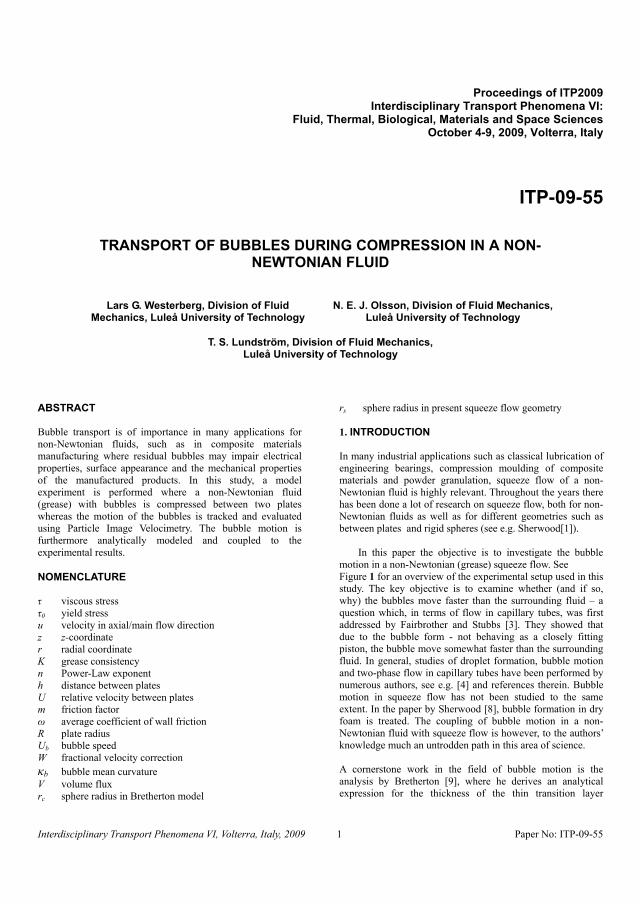
TRANSPORT OF BUBBLES DURING COMPRESSION IN A NON-NEWTONIAN FLUID

Lars G. Westerberg, Division of Fluid Mechanics, Luleå University of Technology

N. E. J. Olsson, Division of Fluid Mechanics, Luleå University of Technology

T. S. Lundström, Division of Fluid Mechanics, Luleå University of Technology

ABSTRACT Bubble transport is of importance in many applications for non-Newtonian fluids, such as in composite materials manufacturing where residual bubbles may impair electrical properties, surface appearance and the mechanical properties of the manufactured products. In this study, a model experiment is performed where a non-Newtonian fluid (grease) with bubbles is compressed between two plates whereas the motion of the bubbles is tracked and evaluated using Particle Image Velocimetry. The bubble motion is furthermore analytically modeled and coupled to the experimental results.

NOMENCLATURE

viscous stress 0 yield stress

u velocity in axial/main flow direction z z-coordinate r radial coordinate K grease consistency n Power-Law exponent h distance between plates U relative velocity between plates m friction factor

average coefficient of wall friction R plate radius Ub bubble speed W fractional velocity correction

b bubble mean curvature V volume flux rc sphere radius in Bretherton model

rs sphere radius in present squeeze flow geometry 1. INTRODUCTION In many industrial applications such as classical lubrication of engineering bearings, compression moulding of composite materials and powder granulation, squeeze flow of a non-Newtonian fluid is highly relevant. Throughout the years there has been done a lot of research on squeeze flow, both for non-Newtonian fluids as well as for different geometries such as between plates and rigid spheres (see e.g. Sherwood[1]).

In this paper the objective is to investigate the bubble motion in a non-Newtonian (grease) squeeze flow. See Figure 1 for an overview of the experimental setup used in this study. The key objective is to examine whether (and if so, why) the bubbles move faster than the surrounding fluid – a question which, in terms of flow in capillary tubes, was first addressed by Fairbrother and Stubbs [3]. They showed that due to the bubble form - not behaving as a closely fitting piston, the bubble move somewhat faster than the surrounding fluid. In general, studies of droplet formation, bubble motion and two-phase flow in capillary tubes have been performed by numerous authors, see e.g. [4] and references therein. Bubble motion in squeeze flow has not been studied to the same extent. In the paper by Sherwood [8], bubble formation in dry foam is treated. The coupling of bubble motion in a non-Newtonian fluid with squeeze flow is however, to the authors’ knowledge much an untrodden path in this area of science. A cornerstone work in the field of bubble motion is the analysis by Bretherton [9], where he derives an analytical expression for the thickness of the thin transition layer


between the bubble and the wall in a pressure driven pipe flow. In this work, the Bretherton solving methodology is applied to a Herschel-Bulkley fluid in squeeze flow geometry. The analytical results covering the bubble motion are coupled to results from experiments for different fluids. The bubble motion is experimentally analyzed using Particle Image Velocimetry (PIV). 2. EXPERIMENTAL Bubbles were observed by visual inspection in initial squeeze flow experiments to move significantly faster than the surrounding non-Newtonian medium. Therefore, the experimental setup was further evolved to render possible flow field measurements with Particle Image Velocimetry (PIV) methodology. During experimenting, two significant behaviours were observed during squeeze flow which will be presented in the results. Firstly, larger bubbles tend to translate faster through the medium than small bubbles. Secondly, bubbles with a higher velocity than the surrounding medium stretches from a circular-like shape into the shape of a falling rain drop, which seems to increase the velocity further. 2.1 SETUP AND PROCEDURE Squeeze flow experiments have been performed with an experimental press which render possible image acquisitions of the flow and associated bubble transport, see Figure 1.

Figure 1: Schematic drawing of the experimental setup. A lump of grease mixed with iron particles, is placed on the lower plate which is pressed towards the upper transparent PMMA plate using the mechanical screwing device. The grease motion is registered by the camera and analysed using PIV software. A grease with non-Newtonian properties was used as fluid, see se §3.1 and Table 1 for data characteristics. In order to facilitate the analysis, PIV was applied to quantify the flow. The basic principle of PIV is to compare sub-images for two master images, recorded with a time interval, with a cross-correlation

algorithm in order to measure how far recognised patterns have travelled between the images (Meinhart et al. [10]). Hence, a velocity vector field can be obtained by adding the results for each sub-image into a master image, see Figure 2 for a schematic drawing of the principle. Since the medium used was homogenous and transparent without cross correlation points, a small amount of particles (iron powder) were evenly distributed in the medium to enable cross correlation. The experimental results presented here contained 7 wt% particles. Moreover, due to the absence of cross-correlation points inside the bubbles, no velocity vectors are obtained within the bubbles. However, since the bubbles affect the surrounding grease, the motion of the bubbles can be estimated for the surrounding flow.

Figure 2: Schematic drawing of the cross-correlation principle. The particle doped grease was placed on the lower plate of the mould to a height of 6.2 mm with aid of a cylinder, with a diameter of 44 mm. The bubbles were then manually added with a syringe and the lower plate was forced to move towards the upper one with the aid of a mechanical screwing device generating a squeezing flow As recording device a Dantec NanoSense MkIII camera was used along with a NIKON 60mm f/2.8D lens, where the image acquisition was controlled by the Motion Studio 2.06.05 software from IDT to 1280x1024 pixel, 8bit and 100 frames per second. The post-processing was performed with the software Dantec Dynamic Studio 2.3 which offered an adaptive cross correlation method, giving more reliable flow fields due to refinement steps through larger sub-images and high accuracy subpixel refinement. In the present case, the final interrogation area size was 8x8 pixel, numerically compiled through 4 refinements steps with 50% overlap from an initial area size of 128x128 pixel. 2.2 RESULTS Experimental results from one designated squeeze flow experiment can be seen in Figure 3-Figure 6, where four different stages are presented in order to demonstrate how the encapsulated bubbles have been affected by the squeeze flow as a function of time. In each figure, three images are presented: the uppermost shows the original recorded image, the middle shows the same image with velocity vectors from the PIV measurements, and in the bottom one a close-up view of the PIV result is presented. Length scales in [mm] can be


seen to the left for respectively magnification and to the right, a colour scale for the vector velocities in [m/s] is placed.

Figure 3: Original, PIV result, and close-up view for stage 1.



A visual inspection of the original images in Figure 3-Figure 6 reveals that a large portion of the encapsulated bubbles in the outer regions are removed during pressing, especially the large bubbles. It can also be seen by inspection of the PIV results, that there is a correlation between areas of increased velocity and position of the bubbles. Comparisons between the original and the PIV image reveal that bubbles having a high velocity relative to the grease, tend to elongates and form a tail which narrows and gives the bubble the shape of a falling raindrop, which further increase the velocity. As a consequence, the grease starts to move inwards towards the bubble tail as seen in the close-up views representing the event history for three bubbles. In the first stage (see Figure 3), the largest bubble, which is also closest to the flow front, has the highest velocity. This bubble seems to affect the bubble above, since the velocity vectors points towards the larger bubble instead of in the radial direction. In the second stage (see Figure 4), the large bubble is elongated and has approached the grease flow front. In the third stage (see Figure 5), the large bubble from the previous stages has escaped the grease which, however, is still affected by its earlier presence since the grease flows towards the area previously occupied by the bubble. Moreover, the other two bubbles have started to elongate, in particular the uppermost which has gained velocity relative to the grease and made a radical approach towards the flow front. As a consequence, grease flows inwards towards the tail as it narrows. In the fourth stage (see Figure 6), this bubble has almost been removed from the grease. The last bubble, which initially had the smallest size of the original three, has formed the shape of a falling raindrop and obtained an increased velocity. Again it can be seen how the grease move inwards towards the tail of the bubble as it narrows. 3. ANALYTICAL MODELING In this section an analytical model for the bubble motion in the grease is sought. 3.1 Grease flow Grease is due to its composition a complex fluid. It consists of a thickener system (usually a metal-soap), base oil and additives. The flow characteristics are dominated by its yield stress behavior, where a critical stress has to be applied in order for the fluid to flow. In a recent study treating grease flow in a rectangular channel, Westerberg et al. [11] showed that the Herschel-Bulkley rheology model can describe the flow well for the greases used in this study. This model is written as

,0

n

zuK (1)


where 0 is the yield stress, K the consistency, and n the Power Law exponent. z is the coordinate perpendicular to the flow direction. Data characteristics for the NLGI2-grease used in this study are presented in Table 1. The NLGI grade indicates the thickness of the grease. As comparison in Table 1, a grease with NLGI grade 1, i.e. a less thick grease, is also presented. The characteristic shear thinning effect – typical for grease, is represented by an n value < 1.

Grease 0 [Pa] K [Pa s]1/n n NLGI1 189 4.1 0.797 NLGI2 650 20.6 0.605

Table 1: Values for the parameters in the Herschel-Bulkley rheology model (Eq. 1). The NLGI2-grease is used in the present study. Values obtained from plate-plate rheometer. From Westerberg et al. [11]. In Westerberg et al. [11] it is shown that there is a very thin shear/slip layer close to the boundaries, where the velocity gradient is very high. Instead of continuously approaching zero velocity at the boundaries, there is a discontinuous behaviour for the velocity in the slip layer. Here we investigate and discuss the influence of this layer on the bubble motion and the original theory by Fairbrother and Stubbs [3] that claims the shape of the bubble as a reason for its different speed; it does not behave like a closely fitting piston in the tube. In contradiction to Newtonian fluids having a parabolic velocity profile, grease take up a plug flow profile where the velocity is constant through a majority of the channel (see Figure 7). The effect of this property is also investigated for its impact on the bubble motion.

Figure 7: Velocity profile for the actual greases across a rectangular channel of width 1.5 mm. Dimensionless velocity

(u) scaled with maximum velocity in the channel. +:NLGI1, ; NLGI2. The third grease (dotted marker) having a Newtonian profile, is a NLGI00 grease. From Westerberg et al. [11]. 3.2 Bubble motion analysis 3.2.1 The Bretherton model Bubble motion in capillary tubes has been studied since the 1930’s when Fairbrother and Stubbs [3] discovered that the velocity of bubbles is slightly higher than the velocity of the surrounding fluid. In his benchmark work, Bretherton [9] showed that the bubble speed Ub exceeds the average speed of the fluid in the tube by an amount UbW, where

.0/ ,29.1/329.1 32

32

UCaCaUW b (2) This result showed to underpredict the thickness of the film formed between the bubble and the tube wall, with a discrepancy being greatest at lowest speeds (Schwartz, Princen and Kiss [12]). However, though the Bretherton theory does not fit experiments in capillary tubes for low speeds, it is a good basis for investigating the bubble motion in the present study. Figure 8 show an overview of a bubble being located between the plates (a) and the situation close to the boundary of one of the plates (b). Using the analogous analysis and notation as Bretherton [9], the bubble geometry and transition layer structure can be directly transferred to the plate-plate geometry following the experiments presented in the previous section. In traditional squeeze flow the two plates move towards each other with identical speed - meaning the origin is fixed in space and located in the middle of the gap between the plates. In the present approach however where the upper plate is fixed in space, the origin is not fixed in space, but moves with the same speed as the lower plate in order to have a fixed coordinate system with respect to the plates. Hence, in terms of this new coordinate system the analysis situation is analogous to traditional squeeze flow. This is most significant when considering the velocity profile in the whole gap between the plates (see Appendix A). For the analysis of the transition layer between the bubble and the plate (see §3.2.2) however, the introduced (local) coordinates are with respect to the plate only. The reason for choosing the upper plate to be fixed in space, is to better and more easily keep focus on the flow when recording it with the camera.

(a)


(b)

Figure 8: Bubble between plates, where the bottom one is moving with velocity U towards the upper plate being fixed in space. (b) Transition region between bubble and lower boundary (cylindrical coordinates). 3.2.2 Transition layer analysis In this section the fractional velocity correction W (Eq. 2) for a Herschel-Bulkley fluid is derived. The analysis follows the methodology by Bretherton [9], where the thin transition layer with thickness b (see Figure 8b) is the subject of investigation. For the transition layer analysis, Bretherton uses the Cartesian coordinates x, y. Here the geometry is cylindrical, and a coordinate transformation is necessary. It is a straightforward approach since no scale factors are introduced when going from (x,y) to (r, z), where r is the radial co-ordinate and z is normal to the plane Considering the bubble/fluid interface (see Figure 8b), zero tangential stress results in

. ,0 1zzz

uz (3)

Normal stress condition at the interface is reduced to

,021

2

11 drzdpp b (4)

applying the lubrication approximation where b is the mean curvature of the bubble (where the curvature of the plate-plate configuration is zero). The Navier-Stokes equation in cylindrical coordinates for a Herschel-Bulkley fluid, and for small Reynolds number, is written as

.01

nr

zuK

zdrdp

(5)

The boundary conditions are determined by the no slip condition at the wall

0 ,0 zur (6)

together with zero tangential stress at the interface (Eq. 3). The volume flux of the fluid is

1

0

,z

r dzuV (7)

where the velocity ur is obtained by integrating Eq. 5, resulting in

2

1/1

11

1

/1 11

),( Czzdrdp

drdpn

nzruKn

rn (8)

using the zero tangential stress B.C. (Eq. 3). Applying the no slip B.C. (Eq. 6) may be written as

.11

),(1/1

11

1/1

11

1

/1n

n

rn

drdpz

zzdrdp

drdpn

nzruK

(9) The resulting volume flux becomes

.121

1

1121

11

,

11/1

1

2/11

/11

/1

1

1/1

11

2/1

11

1

1/1

0

1

zz

znn

drdp

nn

K

zzdrdp

zdrdp

drdpn

n

drdpn

nK

dzuV

n

nn

n

n

n

n

z

r

Differentiating the normal stress condition at the interface (Eq. 4) yields the following expression

,/1

31

3/11

nn

drzd

drdp

(11)

which together with continuity

(10)


czUV b 1 (12) results in

.1113

13

nn

nnb

Kn

nczUdr

zd (13)

Here c and are constants where c is to be determined below, and 1 equals

.1112

1/12/12/111

nnn

nnz (14)

c is determined from the condition

, ,0 131

3

bzdr

zd (15)

which leads to

.bc (16) Eq. 13 can then be written as

,12

21113

13

nnn

nnb zK

nnbzU

drzd

(17)

where

.1112

1/12/12

nn

nn

(18)

Introducing

,13 2* n

n

Kn

n (19)

Eq. 17 then writes as

.321

1

1*

31

3

n

nb

zbzU

drzd

(20)

This equation can be written on universal form by the following variable substitutions:

,3 ,3/1*

32

1b

n Ubrbz (21)

leading to

.1213

3

n

n

dd

(22)

For sufficiently small values of (3μ*Ub/ )1/3 there are regions in which

11

bz

, (23)

resulting in (Eq. 22)

,03

3

(24)

with the solution

.21

322

1 AAA (25)

Returning to the original coordinates (Eq. 20) this solution is written as

.

3321

3

31

3/1*

2321

23/2*

11

bAb

rUAb

rUAz nb

nb

(26) In this region the mean curvature becomes

,13

3211

3/2*

21

2

1s

nb

rb

AUdr

zd (27)

where 1/rs is the mean curvature of a cylinder with radius rs. The surface has constant mean curvature across the plates and can to the first approximation be expressed as a cylinder with radius rs. Eq. 26 and Eq. 27 then yields

.3

1

3/2*321

AU

rb b

s

n

(28)

When n is different from zero it is not straightforward to proceed from this step of the analysis. In region CD (see Figure 8a), z1 approximately equals the transition layer


thickness b, leading to a -value close to unity. This yields (Eq. 22)

,13

3n

dd

(29)

which is not possible to solve analytically for an arbitrary n-values. In this paper the greases have an n-value of approximately 0.6 and 0.8 respectively (c.f. Table 1). So, in order to solve for A1 in Eq. 28, a numerical approach is necessary. Actual values of remaining parameters are however not known at the present stage. To proceed the current analysis, the case n=1 is considered henceforth. In terms of the Herschel-Bulkley rheology model (Eq. 1), this special (Newtonian) case yields the Bingham rheology model which also accounts for the yields stress behavior, but not for the shear thinning/thickening property. How the shear thinning property for the actual greases influences the physics in this study is discussed in §4. 3.2.3 Fractional velocity correction for the plate-plate configuration: Newtonian case (n=1) When n=1, Eq. 28 is written as (c.f. Eq. 19)

,3

1

3/2

AKU

rb b

s

(30)

where A1=0.643 following from the solution to

,13

3

dd

(31)

as shown in the analysis by Breherton [9]. The Bretherton analysis is based on pipe flow geometry (see Figure 9a) with transition layer of thickness b symmetrically near the pipe wall. The fractional velocity correction W as measured by Fairbrother and Stubbs, is the proportion of the cross-sectional area of the pipe occupied by the transition layer [1], i.e.

.329.122 3/2

2

2

2

2b

cccc

c Urb

rb

rb

rbrW

(32) Considering a length l of the plate-plate geometry (Figure 9b), the corresponding proportion is

,3643.022 3/2b

s

KUrb

hb

hlblW (33)

recalling Eq. 30 and that the radius rs approximately is half the distance between the plates h. From Eq. 18 and 19 it is seen that when n equals unity, the introduced apparent viscosity μ* equals K which correspond the viscosity μ of a Newtonian fluid. Hence the result corresponding to n=1 is identical to the result by Bretherton [9], except for a factor two resulting from the change of geometry. Worth noticing is that the yield stress does not affect the solution.

(a)

(b) Figure 9: Cross-sectional view of the transition layer thickness for (a) the pipe flow used by Bretherton [9], and (b) the plate-plate configuration used in this study. 4. DISCUSSION AND COUPLING TO EXPERIMENTS Of certain interest and of vital importance, is to estimate the quality of the performed simplification corresponding to n=1. As measured in the rheometer, the greases used in this paper are shear thinning (n<1). This means that the shear stress decays as the rate of shear is increased - i.e. there is a non-linear relation between the two quantities. For a Newtonian fluid the relation is linear with a shear stress proportional to the shear rate. Furthermore, as shown by Westerberg et al. [11], that for grease it is likely to have a thin shear layer close to the boundaries where the velocity gradient is significantly higher than in the rest of the fluid. Key questions are whether the shear layer and the shear thinning property affect the bubble speed.


From the experimental results presented in §2, it is evident that the bubble speed is higher than for the surrounding grease. The analytical solution yields a velocity fractional correction proportional to the transition layer thickness divided by the mean radius of the bubble. The effective thickness of the layer is found knowing the Capillary number and the curvature radius of the bubble (i.e. approximately the distance between the plates for the squeeze flow case, and the pipe curvature for the pipe flow case). In Bretherton’s experiments [9] a tube with diameter 2 mm was used. In the present study, the distance between the plates at the latter part of the experiment (c.f. Figure 6) where the bubble speed is distinctively higher than the surrounding grease, is of the order of 2 mm. This should be compared to the distance of the order of 4 mm at the initial time of measurement presented in Figure 3, where the bubble speed not differ significantly from the grease speed. As the bubble is highly compressible it is reasonable to assume that the transition layer thickness b between the bubble and the plate wall, remains approximately constant in comparison to the curvature of the bubble which becomes significantly smaller when the plate distance is reduced. According to the relation for the velocity fraction coefficient W in Eq. 33, the value of W then increases. Explicit values of the surface tension and the bubble curvature are not known at present stage. Hence explicit values of the Capillary number are also not known. However, the general behavior for the bubble speed presented in the analysis is to a large extent verified by the experiments. From Eq. 18 and 19 it follows that the introduced apparent viscosity differs from the Newtonian value with a factor directly dependent of the n-value. This factor also affect the solution for z1 and b according to Eq. 21 and 26. For a factor larger than unity, it is not unreasonable to have an increase in the relation b/rs and hence in the bubble speed compared to the surrounding grease. There are several ways to go in order to develop the present study. To study the influence of the non-Newtonian properties, it is of interest to perform the experiments with grease having both thinner and thicker consistency. Furthermore, in order to enhance the coupling to the analytical model, it is of interest to measure the compression (plate) speed, surface tension, and bubble curvature. The natural step of improvement for the analytical model is to make it include a general value of the Power-Law coefficient n. Also, the change of bubble form and how to include this in the model is a subject of great importance. 5. SUMMARY In this paper bubble motion during squeeze flow of a non-Newtonian fluid (grease), is investigated using particle Image Velocimetry (PIV) and an analytical model. The experiments reveal an increase in bubble speed compared to the surrounding grease during the compression (squeeze) of the

plates. During the latter stage of the compression, the particles change form from initially being approximately spherical, to have the characteristic form of a falling raindrop. The change in form coincides with the increase in speed of the bubble. The analytical model is developed from the classical Bretherton analysis [9] for bubbles in pipes. It supports the shown development in the experiments. A full general solution comprising an arbitrary value of the Power Law exponent, for the velocity fraction coefficient representing the relative bubble speed, is however not covered at the present stage.

REFERENCES

[1] J. D. Sherwood and D. Durban, “Squeeze flow of a power-law viscoplastic solid.” J. Non-Newtonian Fluid Mech. 62: 35-54 (1996). [2] J. D. Sherwood and D. Durban, “Squeeze-flow of a Herschel–Bulkley fluid.” J. Non-Newtonian Fluid Mech. 77: 115-121 (1998). [3] F. Fairbrother and A. E. Stubbs, “Studies in electroendomosis Part IV. The bubble-tube method of measurements.” J. Chem. Soc. 1: 527-529 (1935). [4] J. D. Tice, A. D. Lyon and R. F. Ismagilov, “Effects of viscosity on droplet formation and mixing in microfluidic channels.” Analyl. Chem. Acta. 507: 73-77 (2004). [5] P. C. Huzyak and K. W. Koelling, “The penetration of a long bubble through a viscoelastic fluid in a tube.” J. Non-Newtonian Fluid Mech. 71: 73-88 (1997). [6] R. N. Marchessault and S. G. Mason, “Flow of Entrapped Bubbles through a Capillary.” Ind. Eng. Chem. 52(1): 79-84 (1960). [7] A. Serizawa, Z. Feng and Z. Kawara, “Two-phase flows in microchannels.” Exp. Therm. and Fluid Sci. 26: 703-714 (2002). [8] J. D. Sherwood, “Squeeze flow of a dry foam.” J. Non-Newtonian Fluid Mech. 112: 115-128 (2003). [9] F. P. Bretherton, “The motion of long bubbles in tubes.” J. Fluid Mech. 10: 166-188 (1961). [10] C. D Meinhart, S. T. Werely and M. H. B. Gray, “Volume illumination for two dimensional particle image velocimetry.” Meas. Sci. Technol., 11:809–814 (2000). [11] L. G. Westerberg, T. S. Lundström, E. Höglund and P. M. Lugt, ”Investigation of grease flow in a rectangular channel using μPIV.” Trib. Trans. (submitted).


[12] L. W. Schwartz, H. M. Princen & A. D. Kiss, “On the motion of bubbles in capillary tubes.” J. Fluid Mech. 172: 259-275 (1986). [13] H. M. Laun, M. Rady and O. Hassager, “Analytical solutions for squeeze flow with partial wall slip.” J. Non-Newtonian Fluid Mech. 81: 1-15 (1999). APPENDIX A Here solutions for the velocity profile of a Herschel-Bulkley fluid are presented. The velocity development between the plates is not of direct interest in the present approach as it can be treated separately from the flow in the transition layer. However, it is of great interest in general from a fluid mechanical aspect, and the subject for future studies using the μPIV method. In this Appendix a solution for the velocity profile is sought using a methodology analogous to the work by Laun, Rady and Hassager [13]. The governing equations are

,0

01

zdrdp

dzdu

ru

rzr

zr

where

.0

nr

zr zu

K (36)

Integrating (Eq. 34) with respect to r gives

),(zrgur (37) where g(z) is an arbitrary function depending only on the z-coordinate. (ur) in Eq. 35 gives

.0)(2dz

duzg z (38)

Integrating Eq. 36 results in

,)('00nn

nr zgKr

zu

Kdrdpz (39)

using the property

.0 ,0 zzur (40)

Integrating Eq. 39 with respect to r then yields

nn zgr

nKrrpz )('

1)( 1

0 . (41)

As the pressure is not dependent on z, it can be written as an expansion in orders of r such that

... 10

nBrrAp (42) Where A and B are constants. Applying Eq. 42 into Eq. 39 gives after integration with respect to z

,)(')1()1(0nnn zgKrzBrnz (43)

which after integration with respect to z gives

.)1()1(

)1(

11

)(

2

1

0

0

/1

CBznzr

Bnr

nnzgK

nn

n

n

n

Using the partial slip boundary condition

,)(),( sr uRrhrghru (45)

where us is the slip velocity at the boundary, R the radius, and h half the gap distance between the plates, the constant C2 is determined such that

.)1()1(

)1(

11

1

0

0

1

2

nn

n

n

sn

Bhnhr

Bnr

nn

RuKC

which completes Eq. 44. Considering the case n=1 and neglecting the yield stress, g(z) is reduced to Eq. 43 (Power Law fluid) and Eq. 14 (Newtonian fluid) in Laun, Rady and Hassager [13] respectively. Eq. 44 and 46 in Eq. 38 gives after integration

(34)

(35) (44)

(46)


,3

1

120

0

110

0

2

1

1121

1

11

1

11

2

CzRuK

Bzn

zr

nBn

r

zBhnRr

Bnr

nnu

sn

n

n

n

n

n

n

z

where C3 is determined from the boundary condition uz(z=0)=0, giving

.121

11

212

02

03

n

n

n

rn

Bnr

nnC

(48) In order to solve for B, the boundary condition uz(z=h)=dh/dt is utilized, i.e.

.

121

11

22

1

1121

1

11

1

11

2

120

20

1

120

0

110

0

n

n

n

sn

n

n

n

n

n

n

r

nBn

rn

nhRuK

Bhn

hr

nBn

r

hBhnRr

Bnr

nn

dtdh

To solve for B is not possible analytically. However, having explicit numbers on the parameters, a solution for B can be found numerically.

(47)

(49)

Paper C

- 1 -

Compression moulding of SMC: Modelling with CFD and validation

N.E.J. Olsson 1, T.S. Lundström 2, and K. Olofsson 3

1 Division of Fluid Mechanics, Luleå University of Technology, SE-971 87 Luleå, Sweden: [email protected]

2 Division of Fluid Mechanics, Luleå University of Technology, SE-971 87 Luleå, Sweden: [email protected]

3 Swedish Institute of Composites, Swerea SICOMP AB, SE-941 26 Piteå, Sweden: [email protected]

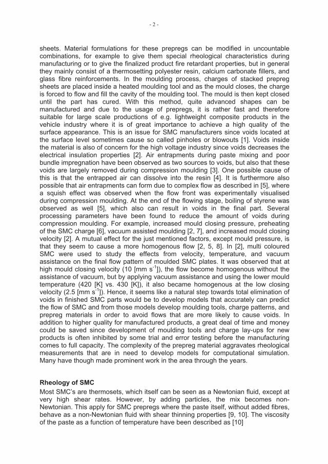
ABSTRACT: Compression moulding experiments of Sheet Moulding Compound (SMC), visual observations of a vacuum test with prepregs, and numerical models for Computational Fluid Dynamics (CFD) for simulations of the present mould filling phase are here presented. The first model sees the flow as only being extensional while the other model sees the flow as mainly extensional but also shearing near the surface of the moulding tool. Pressure comparison with the experiments show that preheating effects can almost be neglected and that the pressure seems to be more accurately predicted if shear layers are present in the viscosity model of SMC. In the experiments it was confirmed that the pressure is predominantly affected by the mould closing velocity during mouldfilling, wherein three phases, separated by two pressure tops, also were observed. Regardless of here applied process settings, the first pressure top always appeared approximately at the logarithmic strain 0.25. The second top was associated with a slow down of the press and a subsequent decrease of the pressure until the applied pressure was reached when the mould was filled. The location at where this occurred was affected by the velocity and the vacuum level. Hence, it is logical to assume that vacuum assistance prevent a build up of back pressure. Furthermore, simple vacuum tests with prepregs indicated that prepreg also desiccate by vacuum, an effect that become more significant for heated prepregs which also swells immediately as vacuum assistance is applied if a critical temperature is reached.

KEYWORDS: SMC, Modelling, CFD

INTRODUCTIONCompression moulding of Sheet Moulding Compound (SMC) is a manufacturing method for composite products. The whole process can briefly be divided into two main steps, preparation and moulding of SMC prepreg, respectively. In the preparation step, prepreg sheets are manufactured which consists of a paste and fibres where the fibres are randomly spread and impregnated in the plane of the

- 2 -

sheets. Material formulations for these prepregs can be modified in uncountable combinations, for example to give them special rheological characteristics during manufacturing or to give the finalized product fire retardant properties, but in general they mainly consist of a thermosetting polyester resin, calcium carbonate fillers, and glass fibre reinforcements. In the moulding process, charges of stacked prepreg sheets are placed inside a heated moulding tool and as the mould closes, the charge is forced to flow and fill the cavity of the moulding tool. The mould is then kept closed until the part has cured. With this method, quite advanced shapes can be manufactured and due to the usage of prepregs, it is rather fast and therefore suitable for large scale productions of e.g. lightweight composite products in the vehicle industry where it is of great importance to achieve a high quality of the surface appearance. This is an issue for SMC manufacturers since voids located at the surface level sometimes cause so called pinholes or blowouts [1]. Voids inside the material is also of concern for the high voltage industry since voids decreases the electrical insulation properties [2]. Air entrapments during paste mixing and poor bundle impregnation have been observed as two sources to voids, but also that these voids are largely removed during compression moulding [3]. One possible cause of this is that the entrapped air can dissolve into the resin [4]. It is furthermore also possible that air entrapments can form due to complex flow as described in [5], where a squish effect was observed when the flow front was experimentally visualised during compression moulding. At the end of the flowing stage, boiling of styrene was observed as well [5], which also can result in voids in the final part. Several processing parameters have been found to reduce the amount of voids during compression moulding. For example, increased mould closing pressure, preheating of the SMC charge [6], vacuum assisted moulding [2, 7], and increased mould closing velocity [2]. A mutual effect for the just mentioned factors, except mould pressure, is that they seem to cause a more homogenous flow [2, 5, 8]. In [2], multi coloured SMC were used to study the effects from velocity, temperature, and vacuum assistance on the final flow pattern of moulded SMC plates. It was observed that at high mould closing velocity (10 [mm s-1]), the flow become homogenous without the assistance of vacuum, but by applying vacuum assistance and using the lower mould temperature (420 [K] vs. 430 [K]), it also became homogenous at the low closing velocity (2.5 [mm s-1]). Hence, it seems like a natural step towards total elimination of voids in finished SMC parts would be to develop models that accurately can predict the flow of SMC and from those models develop moulding tools, charge patterns, and prepreg materials in order to avoid flows that are more likely to cause voids. In addition to higher quality for manufactured products, a great deal of time and money could be saved since development of moulding tools and charge lay-ups for new products is often inhibited by some trial and error testing before the manufacturing comes to full capacity. The complexity of the prepreg material aggravates rheological measurements that are in need to develop models for computational simulation. Many have though made prominent work in the area through the years.

Rheology of SMC Most SMC’s are thermosets, which itself can be seen as a Newtonian fluid, except at very high shear rates. However, by adding particles, the mix becomes non-Newtonian. This apply for SMC prepregs where the paste itself, without added fibres, behave as a non-Newtonian fluid with shear thinning properties [9, 10]. The viscosity of the paste as a function of temperature have been described as [10]

- 3 -

.

TTb

paste e11

00 . (1)

Eq. (1) is often combined with an expression stating that the shear viscosity is a power law function of the shear rate. But it have also been observed that the viscosity of the paste can be described by a Carreau viscosity model [9]. If the viscosity is assumed to be very small at infinitive shear, the Carreau viscosity model can be written as

21

21n

zs(2)

where zs is the zero shear rate viscosity, the time constant, is the shear strain rate and n is the power law constant. This means that the paste behaves as a Newtonian fluid at low shear rates, and as the temperature increases, the Newtonian transition area moves to higher shear rates. It is widely accepted that unreinforced polymers and melts usually have a shear-dominated mould flow and that their flow behaviour can be modelled without considering the extensional viscosity dissipation [11]. However, when modelling materials such as SMC with planar fibre suspensions, it is popular to assume a gapwise velocity profile that is close to a plug flow and that the main viscosity dissipation being in-plane extension since many experiments have shown that SMC deform in a biaxial extensional flow mode with very little mixing between the prepreg layers and extensive slip along the mould walls [12]. It has also been shown that shearing effects can be significant even though the biaxial extension indeed dominates in most cases of fibre suspension squeeze flows [11]. When fibres are added into the plane of sheets, the compression viscosity, or elongation viscosity, is much more affected than the shear viscosity. The compression viscosity of SMC with fibres has been found to be a function of the paste viscosity, Paste and the volume fraction of fibres, added to the paste according to the expression below [10].

ff

f

fn

PastenCompressio ffT

113

1

0

(3)

Where is a constant that was found to be equal to 360, independently of temperature, and is the strain rate ( ). Later, in a subsequent study [13], Eq. (3) was revised into

hh /

2

1000100131

0

ffn

PastenCompressio ffT (4)

which gave a better fit to experiments, especially at low strain rates. It is in the context worth mentioning that the effect of fibres on the shear viscosity is not that dramatic, it have for example been observed that by adding 11.2 volume percent of fibres, the shear viscosity is only increased by a factor of 2.93 [10].

- 4 -

The fibrous microstructure of SMC have been investigated with X-ray phase contrast microtomography and it was observed that the plies before moulding consisted of a core zone with a high amount of fibres between two skins, upper and lower, that consisted of a small amount of fibres [6]. When the charges were moulded, the skins had disappeared for the plies placed inside the charge, creating a core zone with an even and high amount of fibres. However, the skins remained at the upper and lower plies which were in contact with the mould wall. The thickness of the skins remained approximately constant, 0.26 mm for the bottom layer, and 0.22 mm for the upper layer, independently of process settings, placement of charge, and preheat temperature of the charge. This imply that the SMC is highly sheared at the mould walls due to a low viscosity of a compound more or less without fibres and that plug flow models probably can be applied to describe the flow of the core zone [6].

EXPERIMENTAL COMPRESSION MOULDING

Method and Materials Pressure data from compression mouldings were obtained from a process parameter experiments where the altered parameters were vacuum, mould closing speed, and the temperature of the moulding tool. The experiments were performed as a 2-level factorial design experiment with split plot design methodology since it was very time consuming to alter the temperature of the moulding tool, see Table 1 for process settings. Each setting was replicated 4 times, giving a total of 32 samples. The commercial software MiniTab 16 was used to facilitate planning and analysis of the experiments.

Table 1. Settings for the compression moulding experiments. Temperature is on the surface of the lower mould half. The upper surface was 3 °K lower.

Level Low (-1) High (1) Vacuum 0 % 75 % Velocity 2.5[mm s-1] 10 [mm s-1]Temperature 420 [K] 430 [K] Pressure 450 [kN]

An experimental moulding tool of circular geometry with two pressure sensors and with vacuum assistance capability was used for the experiments, see Figure 1. A standard industrial low-profile prepreg was used as experimental material, see Table2 for a summary of the material composition. From this prepreg, circular sheets of diameter 0.16 [m] was prepared. They were thereafter stored in air sealed vessels in order to avoid significant styrene loss before they were randomly picked for the experiments where they were stacked in 7 layers. This resulted in an average height of 14.7 mm. The weight of the stack was controlled before it was placed in the centre of the moulding tool. To increase repeatability and shorten the time that the charge had to lay inside the hot moulding tool before it was moulded, markings were made inside the tool. This facilitated a fast and accurate manual loading of the charge.

- 5 -

Upper mould half

Lower mould half

SMC chargeVacuum vent

Pressure sensors

Figure 1. Schematic illustration of the experimental setup. The radii of the SMC charge and the mould cavity is 80 mm and 159 mm, respectively. As the upper mould half goes down it encapsulates the

cavity which enable the use of vacuum assistance.

Table 2. Composition of the paste. In addition fibres were added to an amount that took up a weight of 26-27 % of the total weight of the paste and fibres.

Resin Mass % Resin 19.3

Low-profile additives 8.9Fillers 66.8

Inhibitor 2MgO 0.77

Internal release agents 1.5Wetting agent 0.46

Experimental results A summary of the experimental pressure response are presented in Figure 2 where each curve is the average pressure response from 4 separate mouldings. As seen in the figure, the pressure rapidly increases until a clear peak forms for the centre pressure sensor approximately at the height of 11.4 mm for both closing velocities. This peak is not as distinct for the outer sensor, instead the increase in pressure is flattened out. The pressure then drops a little at the centre sensor before it then starts to build up again. Interestingly the pressure curves from the outer sensor then border on the ones from the inner sensor indicating that there is a marginal flow and/or very low viscosity flow. During the period visualised in Figure 2, the press was capable of deforming the sample at constant velocity. However, as the press approached the lowest position, it suddenly decelerated and the pressure quickly decreased and finally reached the applied pressure when the press had reached the lowest position and the SMC had completely filled the cavity.

- 6 -

0

10

20

30

40

50

60

70

80

90

3 5 7 9 11 13 15

Height [mm]

Pres

sure

[bar

]

No vacuum, Low temperatureNo vacuum, High temperatureVacuum, High temperatureVacuum, Low temperatureNo vacuum, Low temperatureNo vacuum, High temperatureVacuum, High temperatureVacuum, Low temperature

(a)

0

20

40

60

80

100

120

140

3 5 7 9 11 13

Height [mm]

Pres

sure

[bar

]

15

No vacuum, Low temperatureNo Vacuum, High temperaureVacuum, High temperatureVacuum, Low temperatureNo vacuum, Low temperatureNo Vacuum, High temperaureVacuum, High temperatureVacuum, Low temperature

(b)Figure 2. Average pressure for the 4 replicates at each setting at the low (a) and high (b) mould

closing speed. Solid lines show the pressure readings from the centre sensor and dotted lines show the pressure readings from the outer sensor located at the radii 0.07 m.

Statistical analysis of the experimental results shows several significant results that where found by using a confidence level of 95 %. The results are here divided into two phases during the closing of the moulding tool.

Phase 1 – Start to the first pressure topThe height at where the pressure started to increase, ergo the height where the upper mould half reached the SMC charge, was found to be mainly affected by the vacuum. On average, the pressure for the samples with applied vacuum started to increase 0.64 mm before it started to increase for the samples that were moulded without vacuum assistance. The distance, 0.64 mm is not long, but it was a significant result. Therefore, an additional simple experiment was carried out where prepreg at different temperatures, room temperature, 50 °C, and 80 °C, were placed in a transparent vessel wherein vacuum was applied. For the prepregs at room temperature and 50 °C, nothing extraordinary occurred except that they seemed to dry out after a while. The sample that was preheated to 80 °C, however, immediately and rapidly swelled up when the vacuum was applied. A boiling liquid could also be seen at the surface of the transparent vacuum vessel. It is likely that the observed boiling liquid was styrene that had reached its boiling point due to the applied vacuum [5, 14]. Another significant effect was that the pressure at the first pressure top was mainly affected by the mould closing velocity. No significant effect was found to affect the difference in pressure when the first pressure peak occurred between the two sensors.

Phase 2 – After the first pressure peakThe distance from the first pressure top to the position at where the minimum pressure occurred was found to be significantly affected by the mould closing velocity. At average, the mould had enclosed 1.9 mm further for the slow than for the fast velocity. The distance between the first pressure top and the height at where the pressure reached the same pressure again was manly affected by the velocity. At

- 7 -

average, the press had moved 2.1 [mm] further for the low velocity than for the high before it occurred. The closing velocity of the press was set to go at constant velocity the whole way. However, the press did not manage to do this as discussed previously. According to the statistical analysis there where two main effects, velocity and vacuum, and one interaction effect between velocity and temperature, that affected the height at where the deceleration was initiated. The largest difference was caused by the velocity setting. At the high velocity, the deceleration occurred earlier than at low velocity. The velocity was also involved in an interaction effect with the temperature level. At slow closing velocity, the press was capable to compress the SMC with constant velocity at the same distance for both the high and the low temperature. With the higher closing velocity, the press managed to keep constant velocity further with the higher temperature. Vacuum assistance seemed to aid the press at the end of the moulding phase since the press on average managed to compress the SMC further with constant velocity with applied vacuum assistance. This indicate that vacuum assistance prevent a pressure build up of encapsulated air inside of the moulding tool.

Compression viscosity In [10], a compression viscosity was calculated as

ThresholdnCompressio . (5)

It was found that the result followed a power law. Performing the same operation here with the pressure at the pressure peak registered by the centre sensor for the low and high mould closing velocity and with the average result for each process setting gives the average strain rate sensitivity n=0.33, ranging from 0.28 to 0.36, seeFigure 3.

Figure 3. The compression viscosity at the first pressure peak, derived from average values from each setting. The average n is 0.33, ranging from 0.28 – 0.36.

This result is however not fully trustworthy since a temperature gradient from the moulding tool was present in this work which probably lowers the compression viscosity more for the low closing velocity than for the high velocity due to longer time in contact with the mould before the pressure top was attained. It is therefore

- 8 -

reasonable to assume that if the moulding experiment should have been isothermal, the pressure at the low velocity should have been higher in comparison with the pressure at the high closing velocity than now. As a consequence, n would have approached the expected value 0.3, found from linearization of data in [15]. In [10] a constant strain rate and a homogeneous temperature distribution were applied. Here, the velocity was set to constant which gives an increasing strain rate as the mould closes and the gap between the mould halves decreases. From these results, curves could be plotted, see Figure 4 for one example. In the figure it can be seen that the compression viscosity decreases faster in the beginning, this is probably due to preheating from the moulding tool and the squish effect [5]. At the end, the curve flattens out and n approached the expected value 0.3.

Figure 4. Compression viscosity for a sample from start until the second pressure top seen in Figure2. The highest value occurs at the logarithmic strain 0.25.

NUMERICAL SIMULATION

The commercial software Ansys CFX 12.1 has been used for the simulations. The starting point for this paper was to improve a previously developed viscosity model for CFD simulations of compression moulding of SMC [16].

)( 0)( TTbAeT (6)

With a multiobjective surrogate-based inverse modelling technique Marjavaara et al. managed to obtain simulations that captured the flow behaviour of SMC, and the pressure could successfully be predicted but unfortunately not at two locations simultaneously. Hence, the main goal for his study was to improve the model so that the pressure could be predicted adequately at two locations at the same time. In addition it turned out early that Eq. (6), with only temperature dependence, is not suitable when the mould closing velocity is altered in the experiments as done in the present study. This was not observed in [16] since only one mould closing velocity was used (2 mm/s).

- 9 -

Model Setup Several models were evaluated, and all of them had some geometrical and material properties in common. In the experiments, we have previously shown that there was a pressure top approximately at the same height regardless of processing parameters used. The same behaviour has previously been observed in [10], where it was concluded that the pressure seemed to reach a maximum at the logarithmic strain, = 0.25.( hh /ln 0 ). By observing the SMC charge, it was concluded that the flow of it was initiated after the pressure top [10]. This phenomenon was addressed to air removal. Hence, it is likely that the SMC charge is only compressed until the first pressure top. Therefore, the model is setup to start at 11.4 [mm] which was the average height at where the pressure top occurred. This is actually when =0.25. The cylindrical geometry of the experimental moulding tool is also applied in the numerical model. Since the geometry is axisymmetric, it can be modelled as a slice with symmetry boundary conditions. The slice is, in accordance with the Ansys guidelines, made up of one layer that is extruded 1 degree.

Thermal properties of the material are of great importance, especially when modelling the flow of SMC since the viscosity is directly dependent on the temperature. Thermal conductivity experiments performed on a similar prepreg yielded a value of 0.78 [Wm-

1K-1] during heating up to 80 °C [17]. Later, during cooling from 120 °C to room temperature, the value of 0.98 [Wm-1K-1] was found. The increase was traced to decreased levels of air inside the stack after curing. Therefore, the value 0.78 [Wm-

1K-1] will here be used to reflect the initial conditions in the stack while later during compression the value 0.98 [Wm-1K-1] is applied when much of the air is removed. When calculating these values, the density of the prepreg was measured to 1.816 [g cm-3] and the value 1300 [J kg-1 C-1] was used as specific heat capacity. These data will be applied here as well but, since the stack is assumed to be compressed before the flow is initiated, the density is adjusted to 2.33 [g cm-3].

Heat will be transferred from the tools to the charge before the SMC starts to flow. During the experiment, the charges were placed by hand on the lower mould half before the press were manually started, a process approximated to 5 [s]. In addition we need to account for the time to move the upper mould half down to the height at where the flow is assumed to start, that is = 0.25. In the experimental compression mouldings, the press was programmed to go with very high velocity down to the height 40 [mm], then it slowed down and finally closed at desired constant velocity, 2.5 or 10 [mm s-1]. As a consequence, the preheating time for samples before the actual mould flow was initiated varied between the two mould closing velocities. Initially, this whole time was accounted for before the actual flow actually was initiated in order to obtain accurate initial conditions, see Table 3 for details. However, during the simulations, it could be seen that the overall heat transfer probably was smaller in reality than in the simulation since very large differences in pressure compared to the experiments were predicted for the two velocities when different time was used to simulate the initial temperature in the stack. Instead, when the same initial temperature was used for the two velocities, the temperature became in better agreement with the experiments. It could furthermore also be seen in the simulations that as the time of preheating decreased, the difference in pressure also deceased between the two measuring points, approaching the experimental values. Therefore, the preheating time for the upper and lower side of the SMC were arbitrary set to 0.35 [s] and 1.3 [s], respectively in the final simulations.

- 10 -

Table 3. Initial elapsed time for the heat transfer simulations that were used as initial conditions in the moulding simulations. The time for the lower half is: approximated time from placing the stack inside the mould to start the press+time for the press to reach the upper surface+time to compress the stack to = 0.25.

Velocity [mm s^-1] Lower [s] Upper [s] 2.5 5+12.7+1.3 1.310 5+3.6+0.35 0.35

Two different models for the viscosity have been evaluated. The paste viscosity is assumed to obey the model in equation (1), since it made a nicer fit with the data presented in [9] than equation (6). Fitting equation (1) to the data in [9] gives b the value 11708, significantly higher than reported in [10] and [18] were 4900 and 4500 was found, respectively. The compression viscosity in both models are assumed to follow equation (4) with 0 as 55000 [Pa s] similarly as [10]. The value 0.3 is used for the power law constant n. Hence, the only constant in the models that has been changed during simulation is b. First, a suitable value of b was found for the low velocity and the low temperature for the used pre-heating time. Then the same b was used for the remaining combinations of high and low velocity and temperature at that particular pre-heating time.

Model 1 Due to the common opinion that SMC mainly deforms in extensional flow mode during compression, this model is assumed to only depend on extensional viscosity during flow. The viscosity is based on findings in [10] and [13], where the compression viscosity was described as a function of paste viscosity, strain rate and fibre volume fraction. From [6], the value 0.188 were taken which was the average fibre volume content in the prepreg.

ff

2

1000100131

0

ffn

PastenCompressio ffT (7)

Model 2 Based on the observation in [6], that skins were formed during compression that were highly sheared and an inner core zone with a high volume percent of fibres which seemed to obey extensional flow, a thin layer of shear dominated flow was added to the model, representing the skins. It was observed in [6] that the core had a fibre fraction of 0.2, and that the skins had a ditto of about 0.12. In [10], the shear viscosity was observed to increase by a factor of 2.93 for the fibre fraction 0.112, therefore we simply multiplies the shear viscosity of the paste by 3 in the layers. In order to get rid of problems with shear rates under 1, the Carreau model (Eq. 2) was employed with the static value of 1 for the time constant, giving the curve a power-law-like appearance. Furthermore, the effect of a temperature dependent time constant was tested as well. Here, the data in [9] was used to fit a curve for the time constant. In the core zone, model 1 is still assumed to work. The average thickness of the skins in [6] was in average 0.22 [mm] for the upper one and 0.26 [mm] for the lower one. These thicknesses were unaffected by moulding conditions, the initial prepreg temperature, sample location, and if the prepreg stack were in contact with the mould for 10 [s] before the flow was initiated. The height of the skins in the

- 11 -

present study are for simplicity set to 0.25 [mm]. The viscosity in the core zone obey model 1 (Eq. 7), and the viscosity in the skins is set to follow the following Equation

21

211

0 13 0

nTT

b

Skin e (8)

rty b is matched to get a reasonable rties

ResultsThe modelled pressure for various pressing velocities, preheating times and values on the material property b is here presented. In Figure 5-12, solid lines show the pressure predicted in the centre and dotted lines show the pressure predicted at the radii 0.07 m, representing the location of the outer sensor. The curves named Centre and Outer are the experimental means presented in Figure 2. The preheating time is varied since it was noticed that the initial temperature of the modelled SMC charge highly affected the result while the material propenough initial pressure while the material prope 0 and n were held constant in

duce the number of modelling cases.

decreases. See Figure 5 and Figure 6 where the ressure curves also can be seen when b is adjusted to 7800 for the preheat time 8.6

eorder to re

Model 1For the initial estimated pre-heating times in Table 3 the pressure increases much too rapidly as the mould closes for both closing velocities, see Figure 5 and Figure 6. It can also be seen that the difference in pressure is large between the two points of measurements in comparison with experimental data. However, when the modelled initial temperature for the slow velocity is used, the initial pressure becomes much closer to the experimentally obtained pressure. Hence, it seems like the modelled initial temperature is overestimated even though a lower value of thermal conductivity was used during the period of pure heat transfer. Further modelling reveal that by decreasing the time for the initial temperature modelling, ergo assume that the heat transfer is less than what has been set, the predicted pressure approaches the experimental for both locations since the value of the constant b is allowed to increase as the initial temperaturep[s] (0.35 [s] at the upper surface).

To go one step further it is simulated that the lower surface was heated for 1.3 [s] and the upper surface for 0.35 [s] at the two temperatures 420 and 430 [K] respectively. The result is that for the lower temperature, the simulated pressure follows the experimental results for the low temperature and the low velocity, see Figure 7. But, when the higher temperature was used, the pressure decreased too much as a consequence of the high value of the constant b. For the higher velocity (Figure 8), the pressure increased too rapidly for both temperatures and there was a rather large difference in pressure between the two temperatures. In Figure 7, it can also be seen that the model is sensitive to changes in the value of 0 . By only increasing it to 60 000 [Pa s], the constant b can be increased to 9100, which gives a

t is closer to the experimental values. result tha

Model 2 The modelled pressure for each setting and experimental means can be seen in Figure 9 - Figure 12. The value of the constant b could in this case be dramatically decreased by assuming that the outer layers behave as shear layers. Also for this

- 12 -

model, the predicted pressure came closer to the experimentally obtained pressure if the preheat time was decreased, therefore the preheat time 1.3 [s] for the lower surface and 0.35 [s] for the upper surface was utilized. By assuming that the shear layers have a time constant value of 1, which gives the viscosity curve a power law-like appearance, the constant b could be adjusted to rather low values, see Figure 9and Figure 10. As seen the fit between the predicted pressures and those obtained from the experiments is rather good for both velocities and best for the higher velocity. The low value of b makes the viscosity less dependent on temperature which can be seen for both velocities. In Figure 10 andFigure 11, the predicted pressure can be seen when the time constant is chosen to be a function of the temperature. As a consequence, the shear thinning effect in the layers can almost be neglected due to the high temperature of the SMC in the layers. Therefore, the pressure increase a little too fast for the low velocity (Figure 11), which it also do for the high velocity, but there the initial pressure is too high as well, see Figure 12. The

wer value b, compared to those in model 1, makes the viscosity less temperature dependent and resulting smaller differences in pressure for the two temperatures. lo

-1Figure 5. Model 1 and experimental pressure with velocity 2.5 [mm s ].

- 13 -

Figure 6. Model 1 and experimental pressure with velocity 10 [mm s-1].

Figure 7. Model 1 and experimental pressure with velocity 2.5 [mm s-1].

- 14 -



- 15 -



- 16 -


DISCUSSION

The value of 0 is of course a great source if vagueness, a proper rheological investigation of the paste would have been desirable. The same thing applies for the thickness of the shearing layer. However, both of those material [6, 10] were similar to the one used in these experiments.

The modelling of the initial conditions of the temperature in the stack seemed to overestimate the heat transfer even though a lower number of the thermal conductivity was utilised during this period. When the same initial conditions were used for the two velocities, the pressure approached the experimentally obtained values. Perhaps a more accurate initial condition of the temperature would be to fully neglect preheating effects or in some manner restrict the heat transfer to some limit. Noticeable from the simulations is that as the preheating time is increased, the difference between the pressure readings from the centre and outer pressure increase as well. A more accurate initial condition for the temperature could be found by adjusting the modelled preheating time until the pressure difference in the modelling become equal as it is in the experiments.

In model number 1 [10, 13], shear thinning effects are neglected. However, the high value of b, compared to 4900 and 4500 in [10] and [18], respectively, might cause similar effects as shearing would do. The high values of b applied are not unlikely

- 17 -

and in the same order as the value predicted when fitting Eq. (2) to the data presented in [9] (b=11708).

Model 2 with a time constant equal to 1 showed very good agreement at the high velocity but not as good at the low velocity. It is possible that the time constant should be affected by the temperature, but not as much as in [9] due to the addition of fibres. An effect of this would have been that the shear thinning effect at the low velocity would have decreased due to the increased temperature. This could have made the pressure curve approach the experimental curve.

From this study, it was evident that the viscosity of SMC could not be described by only the temperature as in [16]. However, the approach, multiobjective surrogate-based inverse modelling, may very well be useful if a more advanced viscosity model is to be determined from e.g. model 2, since it turns out that initial conditions and material parameters can be adjusted to get very good fit between simulations and experimental results at different locations in the mould and at different compression speeds.

CONCLUSIONS

From the experiments it is clear that mould closing velocity is the main effect for the pressure. Some kind of yield point that was independent of altered process parameters was found approximately at the logarithmic strain 0.25. The compression viscosity behaves as a power law fluid, but due to the thermal gradients it is not possible to determine the exact value of the power law exponent. Vacuum assistance seems to prevent a pressure build up inside the moulding tool. Heated prepreg (80 °C) momentarily swells as vacuum is applied, hence the full function of vacuum assistance during compression moulding of SMC may be more complex than just removal of air.

The model that seemed most robust in predicting the pressure of the tested models was model number 2, where the SMC obey two deformation modes, extensional flow in the centre (Eq. 7), and shear flow near the surface of the moulding tool (Eq. 8).

ACKNOWLEDGEMENTS

We would like to thank the VINNOVA foundation, participants in the FYS-project for fruitful discussions and material supply, and the staff at Swerea SICOMP.

REFERENCES1. Sjögren, A., An Approach Towards Avoidance of Pinholes and Blowouts in Painted SMC, in

Internationale AVK-TV. 2002: Tagung Baden, Baden. 2. Olsson, N.E.J., T.S. Lundstrom, and K. Olofsson, Design of experiment study of compression

moulding of SMC. Plastics Rubber and Composites, 2009. 38(9-10): p. 426-431. 3. Comte, E., et al., Void formation and transport during SMC manufacturing: Effect of the glass

fiber sizing. Polymer Composites, 2006. 27(3): p. 289-298.

- 18 -

4. Lundstrom, S. and A. Holmgren, Dissolution of Voids During Compression Moulding of SMC.Journal of Reinforced Plastics and Composites, 2009: p. 0731684409336369.

5. Odenberger, P.T., H.M. Andersson, and T.S. Lundstrom, Experimental flow-front visualisation in compression moulding of SMC. Composites Part a-Applied Science and Manufacturing, 2004. 35(10): p. 1125-1134.

6. Le, T.H., et al., X-ray phase contrast microtomography for the analysis of the fibrous microstructure of SMC composites. Composites Part a-Applied Science and Manufacturing, 2008. 39(1): p. 91-103.

7. Yamada, H., et al. Investigation of the Fundamental Causes of Pinholes in SMC Moldings. in 47th Annual Conference, Composites Institute, The Society of the Plastics Industry, Inc. 1992.

8. Kim, D.K., H.Y. Choi, and N. Kim, Experimental Investigation and Numerical-Simulation of Smc in Compression Molding. Journal of Materials Processing Technology, 1995. 49(3-4): p. 333-344.

9. Lee, L.J., L.F. Marker, and R.M. Griffith, The rheology and mold flow of polyester sheet molding compound. Polymer Composites, 1981. 2(4): p. 209-218.

10. Le Corre, S., et al., Shear and compression behaviour of sheet moulding compounds.Composites Science and Technology, 2002. 62(4): p. 571-577.

11. Gibson, A.G. and S. Toll, Mechanics of the squeeze flow of planar fibre suspensions. Journal of Non-Newtonian Fluid Mechanics, 1999. 82(1): p. 1-24.

12. Kia, H.G., ed. Sheet Molding Compounds: Science and Technology. ed. H.G. Kia. 1993, Hanser: Munich. 257.

13. Dumont, P., et al., Anisotropic viscous behavior of sheet molding compounds (SMC) during compression molding. International Journal of Plasticity, 2003. 19(5): p. 625-646.

14. Lundstrom, T.S., B.R. Gebart, and C.Y. Lundemo, Void Formation in RTM. Journal of Reinforced Plastics and Composites, 1993. 12(12): p. 1339-1349.

15. Boylan, S., L.M. Abrams, and J.M. Castro, Predicting molding forces during sheet molding compound (SMC) compression molding. II: Effect of SMC composition. Polymer Composites, 2003. 24(6): p. 731-747.

16. Marjavaara, B.D., S. Ebermark, and T.S. Lundstrom, Compression moulding simulations of SMC using a multiobjective surrogate-based inverse modeling approach. Mechanics of Composite Materials, 2009. 45(5): p. 503-514.

17. Olofsson, K. and E. Sandlund, Mätning av Värmeledningstal i SMC 5412. 2008, SICOMP CR 08-077, Swerea SICOMP AB, Box 271, SE-941 26 Piteå.

18. Dumont, P., et al., Compression moulding of SMC: In situ experiments, modelling and simulation. Composites Part a-Applied Science and Manufacturing, 2007. 38(2): p. 353-368.

Compression Moulding of SMC - DiVA portal999288/... · 2016-09-30 · LICENTIATE THESIS Department...

Documents

Transcript of Compression Moulding of SMC - DiVA portal999288/... · 2016-09-30 · LICENTIATE THESIS Department...