COMPOUND CODES BASED ON IRREGULAR GRAPHS AND THEIR ...

COMPOUND CODES BASED ON IRREGULAR

GRAPHS AND THEIR ITERATIVE DECODING

by

Telex Magloire Ngatched Nkouatchah

University of KwaZulu-Natal

2004

Submitted in fulfilment of the academic requirements for the degree of

Doctor ofPhilosophy in the School ofElectrical, Electronic, and Computer

Engineering, University ofKwaZulu-Natal, 2004.

Abstract

Low-density parity-check (LDPC) codes form a Shannon limit approaching class of

linear block codes. With iterative decoding based on their TaImer graphs, they can

achieve outstanding performance. Since their rediscovery in late 1990's, the design,

construction, and decoding of LDPC codes as well as their generalization have become

one of the focal research points. This thesis takes a few more steps in these directions.

The first significant contribution of this thesis is the introduction of a new class of codes

called Generalized Irregular Low-Density (GILD) parity-check codes, which are

adapted from the previously known class of Generalized Low-Density (GLD) codes.

GILD codes are generalization of irregular LDPC codes, (lnd are shown to outperform

GLD codes. In addition, GILD codes have a significant advantage over GLD codes in

terms of encoding and decoding complexity. They are also able to match and even beat

LDPC codes for small block lengths.

The second significant contribution of this thesis is the proposition of several decoding

algorithms. Two new decoding algolithms for LDPC codes are introduced. In principle

and complexity these algorithms can be grouped with bit flipping algorithms. Two soft

input soft-output (SISO) decoding algorithms for linear block codes are also proposed.

The first algorithm is based on Maximum a Posteriori Probability (MAP) decoding of

low-weight subtrellis centered around a generated candidate codeword. The second

algorithm modifies and utilizes the improved Kaneko's decoding algorithm for soft

input hard-output decoding. These hard outputs are converted to soft-decisions using

reliability calculations. Simulation results indicate that the proposed algorithms provide

a significant improvement in error performance over Chase-based algorithm and

achieve practically optimal perfonnance with a significant reduction in decoding

complexity.

An analytical expression for the union bound on the bit error probability of linear codes

on the Gilbert-Elliott (GE) channel model is also derived. This analytical result is

shown to be accurate in establishing the decoder perfonnance in the range where

obtaining sufficient data from simulation is impractical.

..H

TO GOD BE THE GLORY

111

Dedication

This thesis is dedicated to my father, Elias Nkouatchah, who passed away on November

5, 2002. I thank you for my life and all the love and supported sacrifices you have made

for me. The sense of discipline, independence, hard work, integrity, humility, love and

compassion for all people you awakened and instilled within me at an early age has left

an indelible impression on my life. As a young elementary boy, I remember promising

that I would take my studies all the way and receive a Ph.D. Though I am glad that,

despite the many adversities, I have kept the promise, it is a bitter disappointment that

you did not live long enough to see its completion. No collection of words can express

the deep sense of loss and anger I feel at having lost you prematurely. I am, however,

relieve to know that you are now at peace and will never suffer again.

IV

Preface

The research work discussed in this thesis was performed by Mr. Telex Magloire

Ngatched Nkouatchah, under the supervision of Professor Fambirai Takawira, at the

University of KwaZuluNatal's School of Electrical, Electronic and Computer

Engineering Centre for Radio Access Technologies, which is sponsored by Alcatel and

Telkom South Africa Ltd through the Centre of Excellence Programme.

Parts of this thesis have been presented by the author at the SATNAC 2002 conference

in Drakensberg, South Africa, at the IEEE AFRICON 2002 conference in George,

South Africa, at the IEEE WCNC 2003 conference in New Orleans, Louisiana, U.S.A,

at the SATNAC 2003 conference in George, South Africa, at the SATNAC 2004

conference in Spier Wine Estate, Western Cape, South Africa, at the IEEE AFRICON

2004 in Gaborone, Botswana, and at the IEEE Globecom 2004 conference in Dallas,

Texas, U. S. A. A paper has also been accepted for presentation at the IEEE ICC 2005

in Seoul, Korea. A paper has been published in SAIEEE, and three other papers have

been submitted for review to the journals, "IEEE Transactions on Communications,"

and "IEEE Transactions on Vehicular Technology."

The whole thesis, unless specifically indicated to the contrary in the text, is the author's

work, and has not been submitted in part, or in whole to any other University.

As the candidate's supervisor, I have approved this thesis for submission.

Nan1e: .

Date: .

Signature: ..

v

Acknowledgements

It is impossible to express in words of any length my gratefulness and appreciation to

my supervisor Professor Fambirai Takawira who introduced me to the area of

infOlmation and coding theory. Working with him is a true privilege, and I have

benefited tremendously from his knowledge of science, both in depth and broadness,

and his enthusiasm of doing research. While being a constant source of valuable

insights and advice, he has always allowed me high degree of freedom and

independence to pursue my own research and study. It was, however, his unlimited

encouragement, patience, and availability that kept me focused and made all the

accomplishments in this thesis possible. He is a role model that I can always look up to.

I would like to express my deepest gratitude to Professor Martin Bossert for his

invitation at the department of Telecommunications and Applied Information Theory of

the University of Ulm in Germany, and his readiness to take over the supervision of my

work. I deeply appreciate his insightful ideas and his many hours spent with me

discussing my research.

I would like to thank Dr. Hongju Xu, who has been given me invaluable suggestions

and comments on my research.

My special thanks go to AIcatel and Telkom South Africa for their valued financial

support, to the University of KwaZulu-Natal for the "Doctoral research scholarship",

and to the German Academic Exchange Service (DAAD) for supporting my stay at the

University ofUlm.

I am grateful to all my postgraduate friends for their assistance and for making our time

together enjoyable. Special thanks to Tom Walingo and Dr. Emmanuel Bejide. I thank

our secretaries for their professional help and for their care and kindness. Bruce

Harrison, our system administrator, who devoted great amount of time to maintain the

computers, has been an indispensable resource for my work.

Vi

Above all, I would like to express my greatest gratitude and sincere appreciation to my

family and friends for their support, understanding, love and trust.

Vll

Table of Content

ABSTRACT 11

DEDICATION IV

PREFACE V

ACKNOWLEDGEMENTS VI

TABLE OF CONTENT VIII

LIST OF TABLES XIII

LIST OF FIGURES XIV

ACRONYMS AND NOTATIONS XIX

CHAPTER 1 1

INTRODUCTION 1

1.1 Coding for Digital Data Transmission 1

1.2 Shannon Linlit. 2

1.3 Two Classes of Shannon Limit Approaching Codes 3

1.4 Thesis Objective and Outline 4

1.5 Original Contribution in the Thesis 7

1.6 Published Work 8

CHAPTER 2 11

LOW-DENSITY PARITY-CHECK CODES 11

2.1 LDPC Structure 12

2.1.1 Definition of Low-Density Parity-Check Codes 12

2.1.2 Analytical Properties ofLDPC Codes 15

2.1.2.1 LDPC Codes with j = 3 are Asymptotically Good 15

2.1.2.2 LDPC Codes with j = 2 are not Asymptotically Good 17

2.2 Graphical Representation 19

Vlll

2.3 Irregular Low-Density Parity-Check Codes 21

2.4 Construction of Low-Density Parity-Check Codes 23

2.4.1 Random Construction 23

2.4.2 Algebraic Construction 24

2.4.2.1 Construction Based on Finite Geometries 24

2.4.2.2 Construction Based on Reed-Solomon (RS) Codes 26

2.4.2.3 Construction Based on Combinatorial Designs 26

2.4.2.4 Construction Based on Circulant Decomposition 26

2.4.2.5 Construction Based on Graphs 27

2.5 Conclusion 27

CHAPTER 3 28

DECODING OF LOW-DENSITY PARITY-CHECK CODES 28

3.1 Introduction 28

3.2 Review of Existing Decoding Algorithms 30

3.2.1 Majority-Logic Decoding 30

3.2.2 Bit Flipping Decoding 34

3.2.3 Weighted Majority-Logic and Bit Flipping Decodings 36

3.2.4 Improved Weighted Bit Flipping Decoding 38

3.2.5 Iterative Decoding based on Belief Propagation or Sum-Product

Algorithm 42

3.2.5.1 Reduced Complexity Iterative Decoding 45

3.3 Two New Decoding Algorithms for Low-Density Parity-Check Codes 47

3.3.1 Notation and Basic Definitions 48

3.3.2 Algorithm I 49

3.3.3 Algorithm II 49

3.3.4 Loop Detection 51

3.3.5 Computational Complexity 53

3.4 Simulation Results 54

3.4.1 Perfonnance of Algorithm 1. 54

3.4.2 Impact ofSNR on the Optimal Value of a in Algorithm IJ 54

3.4.3 Impact of Column Weight on the Optimal Value of a in Algorithm 11 55

IX

3.4.4 Impact of the Value of a on the Average Number of Iterations in

Algorithm 11 55

3.4.5 Perfonnance of Algorithm II With Optimal a 55

3.5 Conclusions 69

CHAPTER 4 70

GENERALAZATION OF IRREGULAR LOW-DENSITY PARITY-CHECK

CODES 70

4.1 Introduction 71

4.2 Definition and Construction of GILD Codes 72

4.2.1 Definition 72

4.2.2 Construction 72

4.3 Ensemble Performance 74

4.3.1 Average Weight Distribution of GILD Codes 75

4.3.2 Lower Bound on the Asymptotic Minimum Distance 77

4.3.3 BSC Channel Threshold 85

4.4 Upper Bound on Minimum Distance for a Fixed Length 91

4.5 GILD Codes Based on Different Constituent Codes 93

4.5.1 Definition 93

4.5.2 Contruction 94

4.5.3 Ensemble Performance 95

4.6 ML Decoding Error Probability over the AWGN Channel 97

4.6.1 Union Bound 97

4.6.2 Improved Bound Based on Gallager's Bound 98

4.6.3 Tangential Sphere Bound 99

4.7 Decoding of GILD Codes 101

4.7.1 MAP Decoding of Linear Block Codes 102

4.7.2 Chase-Based Decoding Algorithm 103

4.7.3 Iterative Decoding of GILD Codes 104


4.9 Conclusions 112

CHAPTER 5 113

x

A LOW-WEIGHT TRELLIS-BASED SOFT-INPUT SOFT-OUTPUT

DECODING ALGORITHM FOR LINEAR BLOCK CODE. 113

5.1 Introduction 114

5.2 Preliminaries 115

5.3 Low-Weight Trellis Diagram 116

5.4 Low-Weight Trellis Diagram Using Supercodes 121

5.5 A Low-Weight Soft-Input Soft-Output Decoding Algorithm 122


5.7 Conclusion 126

CHAPTER 6 127

HIGH-PERFORMANCE LOW-COMPLEXITY DECODING OF

GENERALIZED LOW-DENSITY PARITY-CHECK CODES 127

6.1 Introduction 128

6.2 Structure ofGLD Codes 129

6.3 Proposed Algorithm 131

6.3.1 Soft Decision Decoding of Linear Block Codes Using the Improved

Kaneko Algoritru11 131

6.3.2 Test Error Patterns 135

6.3.3 Soft-Input Soft-Output Decoding of Linear Block Codes Using the

Improved Kaneko algorithm 138

6.3.4 Iterative Decoding ofGLD Codes 141

6.3.5 Decoding Complexity 143

6.4 Stopping Criteria for GLD Decoding 144

6.5 Simulation Model and Results 145

6.6 Conclusions 157

CHAPTER 7 158

UNION BOUND FOR BINARY LINEAR CODES ON THE GILBERT-ELLIOTT

CHANNEL MODEL WITH APPLICATION TO TURBO-LIKE CODES 158

7.] Introduction 159

7.2 The Gilbert-Elliott Channel Model. 160

Xl

7.3 Matching the Gilbert-Elliott Channel Model to the Land Mobile Channel.. 163

7.4 Pairwise Error Probability on the Gilbert-Elliott Channel.. 168

7.5 Application to Turbo Codes 171

7.6 Application to GLD Codes 172

7.6.1 Average Weight Distribution of GLD Codes 172

7.6.2 Union Bound on the Bit-Error Probability of GLD Codes on the GE

Chmmel 174

7.6.3 GLD Decoder for the Gilbert-Elliott Cham1el 174

7.7 Simulation Model and Numerical Results 175

7.8 Conclusion 182

CHAPTER 8 183

CONCLUSION 183

8.1 Summary 183

8.2 Future Work 184

.APPENDIX A 186

APPENDIX B 188

APPENDIX C 189

REFERENCES 191

XlI

List of Tables

Table 2.1: Gallager's construction of the parity-check matrix of a (20, 3, 4) regular

LDPC code C 14

Table 3.1: Decoding Complexity per Iteration 53

Table 3.2: Different LDPC codes simulated 56

Table 3.3: Impact of Column Weight on the Optimal a in Algorithm II for Different

LDPC Codes 62

Table 4.1: Asymptotic lower bounds on the normalized minimum hamming distance 6

of some GILD Codes compared with the Gilbert-Varshamov bound 60

, *

indicates that 6 does not exist. 84

Table 4.2: BSC crossover probability threshold p of some GILD codes compared with

the threshold P(C) of the code of the same rate achieving capacity 92


of some GILD Codes based on two different constituent codes compared

with the Gilbert-Varshamov bound 60

, * indicates that 6 does not exist. . 97

Table 5.1: State complexity profile for the full trellis and two subtrellises of the (31, 21,

5) BCH code 120

Table 6.1: An example of decoding procedure for (15, 7, 5) BCH code using the lKA.

.................................................................................................................... 135

Table 6.2: An example of decoding procedure for (15, 7, 5) BCH code of example 3.1

using the IKA with the preprocessing test. 138

Xlll

List of Figures

Figure 2.1: Properties of the parity-check matrix H of regular LDPC codes 12

Figure 2.2: Average asymptotic values of the normalized Hamming distance of the

ensemble of LDPC codes 17

Figure 2.3: Dependency graph of an LDPC code with j = 2 and k = 3 18

Figure 2.4: Graphical representation of an LDPC code with parameters (N,j,k) as a

Tanner random code 20

Figure 3.1: Bit-error-rate of the (2048, 1723) RS-LDPC code with parameters

r = 6, P = 32 based on different hard-decision decoding algorithms 57


r = 3, P = 16 based on different hard-decision decoding algorithms 58

Figure 3.3: Impact of the weighting factor a in Algorithm II on the BER performance

for the decoding of the (2048, 1664) PEG-LDPC code with parameters

r=3, p=16 59


for the decoding of the (2048, 1664) PEG-LDPC code with parameters

r =6, P =32 60


for the decoding of the (2048, 1723) RS-LDPC code with parameters

r=6, p=32 61

Figure 3.6: Impact of the weighting factor a in Algorithm II on the average number of

iterations of the (2048, 1664) PEG-LDPC code with parameters

r = 3, P = 16 63

Figure 3.7: Bit-error-rate of the Type-I 2-D (1023, 781) EG-LDPC code with

parameters r =32, P =32 based on different soft-decision decoding

algoritmns 64

XIV


r = 6, p = 32 based on different soft-decision decoding algorithms 65

Figure 3.9: Bit-en-or-rate of the (2048, 1649) RS-LDPC code with parameters



r =10, P = 32 based on different soft-decision decoding algorithms 67

Figure 3.11: Bit-error-rate of the (2048, 1664) PEG-LDPC code with parameters


Figure 4.1: Example of a low-density matrix of a GILD code for N = 20, n = 4, and

() = 0.8 74

Figure 4.2: Average weight distribution of a GILD code of length N = 961, () = 0.903

based on the (31, 21, 5) BCH code, compared with the binomial

approximation 77

Figure 4.3: lol"(s) for a GILD code based on the (31, 21, 5) BCH component code. () =

0.903 82

Figure 4.4: B(In/''' s) plotted as a function of 10

1'1 for the GILD code based on the (31,

21,5) BCH component code. () = 0.903 83

Figure 4.5: En-or vector e and codeword c .. The 1s of each vector are drawn at the first---:/

positions of the vectors to help understanding 86

Figure 4.6: Upper bounds using (4.71) for GILD codes based on the (31, 21, 5) BCH

component code 94

Figure 4.7: Illustration of the tangential sphere bound 101

Figure 4.8: Simulated performance of four GILD codes and the con"esponding GLD

code built from the (31,21,5) BCH constituent code, length N = 961,

AWGN channel. 106

Figure 4.9: Simulated perfonnance of three GILD codes and the corresponding GLD

code built from two different constituent codes. The (31,21,5) BCH (used

xv

III the first super-code) and the (31,26,3) Hamming code (used in the

second super-code), length N = 961, AWGN channel.. 107

Figure 4.10: Simulated performance of two GILD codes and the corresponding GLD

code built from two different constituent codes. The (31,26,3) Hamming

code (used in the first super-code) and the (31,21,5) BCH code (used in the

second super-code), length N = 961, AWGN channel.. 108

Figure 4.11: Simulated perfonnance of a GILD code of length N =1005 and rate

0.491 (B = 0.910) built from the (15,11,3) Hamming code and two LDPC

codes of length N =1008 and rate 0.5, AWGN chmmel. 110

Figure 4.12: Bit Error Probability upper bounds and simulations results for the GILD

code based on the (31, 21, 5) BCH component code. e = 0.903 111

Figure 5.1: Simulated performance of the GILD code of length N = 961, e = 0.806,

built from the (31, 21, 5) BCH component code, AWGN channel, 8

iterations 124

Figure 5.2: Performance of the simulated GILD Llsing the proposed algorithm with p =

7 (solid) and the MAP algorithm applied to the full trellis (dashed) after 8

iterations in both cases. N = 961, 8 = 0.806, built from the (31, 21, 5) BCH

component code, AWGN channel. 125

Figure 5.3: Performance of the simulated GILD code using the proposed algorithm

(dashed) and the chase-based algorithm (solid) after 8 iterations in both

cases. N = 961, 8 = 0.806, built from the (31, 21, 5) BCH component code,

AWGN channeL 126

Figure 6.1: Structure of a GLD parity-check matrix 130

Figure 6.2: The q-th GLD decoding iteration 143

Figure 6.3: Performance of the proposed decoding algorithm for different number of

iteration (for Code 1). Maximum NBDD for each iteration = 16 148

XVI

Figure 6.4: Perforn1ance of code 1 using the proposed algorithm and the chase-based

algorithm after 8 iterations in both cases. The number of error pattern

generated in both algorithms was made equal to 16 149

Figure 6.5: Comparison of the average number of bounded-distance decoding used by

the proposed algorithm and the Chase-based algorithm for the same number

of error patterns generated (NI' = 16). Code 1. 150

Figure 6.6: Perfonnance of code 1 using the proposed algorithm and the chase-based

algorithm after 8 iterations in both cases. The maximum number bounded

distance decoding for each iteration in both algorithms was made equal to

16 151

Figure 6.7: Percentage of positions using the theoretical value of beta (case 1) for

different BERs after decoding for the proposed algorithm and the Chase-

based algorithm. Code 1 152

Figure 6.8: Comparison of the number of error patterns generated by the two decoding

algorithms for the same number of bounded-distance decoding ( N BDD = 16).

Code 1 153

Figure 6.9: Simulated BER performance for the two terminating schemes and the fixed

method using the proposed algorithm. Maximum NBDD = 16 for each

iteration. Code 1 154

Figure 6.10: Simulated average number of iterations for the two terminating schemes

and the fixed method using the proposed algorithm. Maximum NBDD = 16

for each iteration. Code 1 155

Figure 6.11: PerfOlmance comparison of the trellis-based MAP algorithm and the

proposed algorithm for code 2. 8 iterations 156

Figure 7.1: The Gilbert-Elliott channel model... 160

Figure 7.2: Physical interpretation of the states in the Gi1bert-Elliott model. 161

Figure 7.3: Good state binary symmetric channel 162

Figure 7.4: Bad state binary symmetric channel. 162

XVII

Figure 7.6: Bounds on the bit error rate of 1/3 rate turbo code for various block lengths

N, /m = 0.1 (lower group), and/m = 0.03 (upper group) 176

Figure 7.7: Bounds on the bit error rate of 1/3 turbo code for various values of the

threshold, /m = 0.1 177

Figure 7.8: Transfer function bound versus simulations results for 1/3 rate turbo code,

/m = 0.1 178

Figure 7.9: Transfer function bound versus simulation results for 1/3 rate turbo code,

/m = 0.03 179

Figure 7.10: Transfer function bound versus simulation results for J = 2 GLD code with

Hamming (15, 11, 3) constituent code. N = 420, /,,, = 0.1. 180


Hamming (15,11,3) constituent code. N= 420, /,,, ~ 0.03 181

XVIII

Acronyms and Notations

The main acronyms and notations used in this document are presented here. We try to

keep consistent and homogeneous notations in the entire report. However, in some rare

places, notations do not have their general meaning summarized here. Normally,

acronyms are recalled the first time they appear in any chapter.

Acronyms

APP A Posteriori Probability

AWGN Additive White Gaussian Noise (channel)

bps bit per second

BCH Bose-Chaudhuri-Hocquenghem (code)

BCJR Bahl Cocke Jelinek Raviv

BER Bit Error Rate

BF Bit Flipping

BIAWGN Binary Input Additive White Gaussian Noise

BIBD

BPSK

BSC

DMC

EG

FEC

GE

GF

GILD

GLD

GV

HAD

IDBP

IHAD

iid

Balanced Incomplete Block Design

Binary Phase Shift Keying (modulation)

Binary Symmetric Channel

Discrete Memoryless Channel

Euclidean Geometry

Forward Error Correction

Gilbert-ElIiott (channel)

Galois Field

Generalized Irregular Low Density (code)

Generalized Low density (code)

Gilbert-Varshamov (bound)

Hard Decision Aided

Iterative Decoding Based on Belief Propagation

Improved Hard Decision Aided

independent and identically distributed

XIX

lKA

IOWEF

IWBF

KA

LDPC

LLR

MAP

MDS

ML

MLG

pce

pdf

PEG

RS

SDR

SNR

SPA

spc

SISO

SOYA

SNR

UMP

VA

WBF

WMLG

Improved Kaneko Algorithm

Input-Output Weight Enumerator Function

Improved Weighted Bit Flipping (decoding)

Kaneko Algorithm

Low Density Parity Check (code)

Log Likelihood Ratio

Maximum a posteriori (decoding)

Maximum Distance Separable

Maximum Likelihood (decoding)

Majority Logic (decoding)

parity check equation

probability density function

Progressive Edge Growth

Reed Solomon

Sign Difference Ratio

Signal to Noise Power Ratio

Sum Product Algorithm

single parity check (equation)

Soft-Input Soft-Output (decoder)

Soft-Output Viterbi Algorithm

Signal-to-Noise Ratio

Uniformly Most Powerful

Viterbi Algorithm

Weighted Bit Flipping (decoding)

Weighted Majority Logic (decoding)

Notations

f.-; If not specified, the i-th bit of the considered codeword

f.-, If not specified, the j-th codeword of the considered code

C, If not specified, a codeword of weight I

xx

c

n

N

N(l)

N(l)

Nal2

~\I'

r

R

If not specified, the considered compound code

The minimum Hamming distance of the considered code

Carrier Frequency Energy per information bit

Signal to Noise Ratio per information bit

If not specified, the dimension of the considered constituent code

If not specified, the dimension of the considered compound code

If not specified, the weight of the considered codeword

If not specified the length of the considered constituent code

If not specified, the length of the considered compound code

Weight distribution of the considered code

Average weight distribution of the considered ensemble of codes

Two sided Power Spectral Density of the AWGN

Bit Error Probability (or BER)

Word Error Probability

If not specified, the rate of the considered constituent code

If not specified, the rate of the considered compound code

XXi

CHAPTERl

INTRODUCTION

With the advance of digital logic design, the last decade has observed wide application

and deployment of digital communication and error protection techniques. These

techniques have enabled, and induced explosive demands for, high-quality and high

speed voice-band modems, digital subscriber loops, personal wireless communications,

mobile and direct-broadcast satellite communications. To achieve efficient use of

bandwidth and power and, at the same time, combat against adverse channel conditions,

new engineering challenges have arisen. For example the systems should have low

physical and computational complexity to increase portability and reachability, allow

seamless data rate changes to cope with time-varying channel conditions and higher

level network protocols, and provide unequal error protection to accommodate different

service rates and to differentiate bits of nonuniform importance from advanced source

encoders. In this thesis, new high-performance error correcting techniques with low

system complexity are developed to address these new challenges.

1.1 Coding for Digital Data Transmission

The ever increasing information transmission in the modem world is based on reliably

communicating messages through noisy transmission channels; these can be telephone

lines, deep space, magnetic storing media, etc. Error-correcting codes play a significant

role in correcting errors incurred during transmission; this is carried out by encoding the

message prior to transmission and decoding the corrupted received codeword for

retrieving the original message.

The performance of a coded communication system IS usualIy measured by its

probability of decoding elTor called error probability. There are two types of error

1

probability. Probability of word (frame or block) error is the probability that a decoded

codeword at the output of the decoder is in error. This error probability is commonly

called word error rate (WER), frame error rate (FER), or block error rate (BLER).

Probability of bit error is the probability that a decoded information bit at the output of

the decoder is in error. This error probability is commonly called bit error rate (BER).

Another performance measure of a coded communication system IS coding gam.

Coding gain is defined as the reduction in the required signal-ta-noise ratio (SNR) to

achieve a specific error probability for a coded communication system compared to an

uncoded system that transmit information at the same rate. SNR is defined as the ratio

of the average power of the demodulated message signal to the average power of the

noise measured at the receiver output.

1.2 Shannon Limit

The fundamental approach to the problems of efficiency and reliability in

communication systems is contained in the Noisy Channel Coding Theorem developed

by C. E. Shannon [1] in 1948. Shannon's theorem states that over a noisy channel, if the

transmission rate R, constituted by the ratio between the number of bits in the original

message and the transmitted codeword, is less than the channel capacity C, there exists a

coding scheme of code rate R that achieves reliable communication. Specifically, for

every rate R < C, there exists at least one good code sequence with probability of error

approaching zero while the blocklength, N, approaches infinity. Furthem10re, he proved

that the probability of error is bounded away from zero if the transmission rate is greater

than capacity, no matter how large N is. Shannon's chmmel coding theorem clearly

states that chmmel capacity is a dividing point: at rates below capacity, the probability

of error goes to zero exponentially; at rates above capacity, the probability of error goes

to one exponentially. The proof to the theorem is essentially non-constructive. It shows

that for long block length, almost all codes of rate R « C) would be reliable. However,

it does not give an explicit construction of capacity-approaching codes, nor does it lay

out practical decoding algorithms. Ever since, coding theorists have been trying to find

codes that would achieve Shannon's theoretical limit. Besides good elTor perfonnance,

2

the codes for pratical applications must have realizable and preferably small encoding

and decoding complexity.

1.3 Two Classes of Shannon Limit Approaching Codes

In the 50 years since Shmllion determined the capacity of ergodic noisy channels, the

construction of capacity-approaching coding schemes that are easy to encode and

decode has been the supreme goal of coding research. In the last decade, a breakthrough

was made in this field with the discovery of some practical codes and decoding

algoritlllils which approach considerably the ultimate channel capacity limit. There are

two large classes of such codes.

In 1993, Berrou, Glavieux, and Thitimajshima [2] [3] introduced turbo codes to the

world. They showed that turbo codes provide capacity approaching performance with

suboptimal iterative decoding. These results caused an increased interest in iterative

decoding methods and iteratively decidable codes. Further research led to the

rediscovery of another powerful class of iteratively decodable codes, low-density parity

check (LDPC) codes, by Sipser et al. [9], MacKay et al. [10], and Wiberg [11].

Turbo codes are obtained by parallel or serial concatenation of two or more component

codes with intrleavers between the encoders. The component codes are mainly simple

convolutional codes. Therefore, it is easy to construct and encode turbo codes. As

mentioned, an interleaver is required to permute the input infonnation sequence. It is

shown that the larger the interleaver size, the better the performance of turbo codes. On

the other hand, large interleaver causes large decoding delay. In decoding of a turbo

code, each component code is decoded with a trellis based algorithm. Therefore, for

practical implementations, only codes with simple trellises can be used as component

codes of turbo codes. However, codes with simple trellises normally have small

minimum distances, causing the error floor at medium to high SNR. In turbo decoding,

at each decoding iteration the reliability values and estimates are obtained only for the

infomlation bits. Thus no error detection can be performed to stop the decoding

iteration process. The only way to stop the decoding is to test the decoding

3

convergence, which is usually complex. No error detection results in poor block error

rate and slow termination of iterative decoding.

LDPC codes are block codes. They were discovered by Gallager in early 1960's [2] [3].

After their discovery, they were ignored for a long time and rediscovered recently. It has

been proved that LDPC codes are good, in the sense that sequences of codes exist

which, when optimally decoded, achieve arbitrarily small error probability at nonzero

communication rates up to some maximum rate that may be less than the capacity of the

given channel. Numerous simulation results showed that long LDPC codes with

iterative decoding achieve outstanding performance. Until recently, good LDPC codes

were mostly computer generated. Encoding of these computer generated codes is

usually very complex due to the lack of understanding their structure. On the other

hand, iterative decoding for LDPC codes is not trellis based, and it is not required for

LDPC codes to have simple trellises. Thus, their minimum distances are usually better

that those of turbo codes. For this reason, LDPC codes usually outperform turbo codes

in moderate to high SNR region and exhibit error floor at lower en'or rates. Another

advantage of LDPC codes over turbo codes is that their decoding algorithm provides

reliability values and estimates for every code bit at the end of each iteration, enabling

error detection. The decoding iteration process is stopped as soon as the estimated

sequence is detected as a codeword. Therefore, LDPC codes nom1ally provide better

block error performance and faster termination of the iterative decoding.

1.4 Thesis Objective and Outline

This thesis deals firstly with the design of concatenated codes and reduced complexity

iterative decoding algorithms, and secondly with the characterization of codes in

channels with memory.

The thesis is organized in such a way that different chapters can be read independently.

The outline for the remainder of the thesis is as follows. In Chapter 2, the construction

of the original regular LDPC codes is briefly recalled. Their analytical properties as

derived by Gallager are reviewed. Their graphical representation as Tanner codes on

4

random graphs are also presented, and a review of the different construction methods is

given. The chapter does not claim to be self-contained but its aim is rather to be an

introduction for the generalized irregular low-density (GILD) codes presented in

Chapter 4, whose construction is inspired by irregular LDPC codes and generalized

low-density (GLD) codes, and that share the common properties with them.

In Chapter 3, different existing decoding methods used for decoding of LDPC codes are

described and two new decoding algorithms are presented. The first algorithm is a hard

decision method, and the second one is a modification of the first to include reliability

information of the received symbols. In principle and in complexity, the algorithms

belong to the class of so called bit flipping algorithms. The defining attribute of the

proposed algorithms is the bit selection criterion which is based on the fact that, for low

density matrices, the syndrome weight increases with the number of errors in average

until error weights much larger than half the minimum distance. A loop detection

procedure with minimal computational overhead is also proposed that protects the

decoding from falling into infinite loop traps. Simulation results show that the proposed

algorithms offer an appealing performance/cost trade-offs and may deserve a place in an

LDPC decoding "toolbox".

In Chapter 4, a new class of codes called generalized irregular low-density (GILD)

codes is presented. This family of pseudo-random error correcting codes is built as the

intersection of randomly permuted binary codes. It is a direct generalization of irregular

LDPC codes, and is adapted from the previously known class ofgeneralized low density

(GLD) codes introduced independently by Lentmaier et al.[22], and Boutros et al. [23].

[t is proved by an ensemble performance argument that these codes exist and are

asymptotically good in the sense of the minimum distance criterion, i.e. the minimum

distance grows linearly with the block length. Upper and lower bounds on their

minimum Hamming distance are provided, together with their maximum likelihood

decoding error probability. Two iterative soft-input soft-output decoding for any GILD

code are presented, and iterative decoding of GILD codes for communication over an

AWGN channel with binary antipodal modulation (BPSK) is studied. The results are

compared in tenns of performance and complexity with those of GLD codes. The high

5

flexibility in selecting the parameters of GILD codes and their better performance and

higher rate make them more attractive than GLD codes and hence suitable for small and

large block length forward error correcting schemes. Comparison between simulation

results of a GILD code and the best LDPC code of length 1008 and rate 0.5 shows very

close performances, suggesting that variations of GILD codes may be able to match or

beat LDPC codes for small block lengths.

In Chapter 5, reduced-complexity trellis-based soft-input soft-output (SISO) decoding

of linear block codes is considered. A new low-weight subtrellis based SISO decoding

algorithm for linear block code to achieve near optimal error performance with a

significant reduction in decoding complexity is presented. The proposed scheme is

suitable for iterative decoding and has the following important features. An initial

candidate codeword is first generated by a simple decoding method. A low-weight

subtrellis diagram centered around the candidate codeword is constructed. The MAP

algorithm is then applied to the subtrellis. The generated extrinsic information is used as

apriori information to improve the generation of a candidate codeword for the next stage

of iteration. Simulation results indicate that the proposed algorithm provides a

significant improvement in elTor performance over Chase-based algorithm and achieves

practically optimal performance with a significant reduction in decoding complexity.

In Chapter 6, an efficient list-based soft-input soft-output (SISO) decoding algorithm

for compound codes based on linear block codes is presented. Attention is focused on

GLD codes. The proposed algorithm modifies and utilizes the improved Kaneko's

decoding algorithm for soft-input hard-output decoding. These hard outputs are

converted to soft-decisions using reliability calculations. Compared to the trellis-based

Maximum a Posteriori Probability (MAP) algorithm, the proposed algorithm suffers no

degradation in performance at low bit-error rate (BER), but presents the major

advantages of being applicable in cases where the trellis-based MAP algorithm would

be prohibitively complex and impractical. Compared to the Chase-based algorithm of

[85], [86], [88], [89] the proposed algorithm is more efficient, has lesser computational

complexity for the same performance and provides an effective tradeoff between

performance and computational complexity to facilitate its usage in practical

6

applications. To improve the average decoding speed of the GLD decoder, two simple

criteria for stopping the iterative process for each frame immediately after the bits can

be reliably decoded with no further iterations are proposed.

In Chapter 7, an analytical expression for the pairwise error probability of maximum

likelihood decoding of a binary linear code on the Gilbert-Elliott (GE) channel model is

derived. This expression is used to obtain the union bound on the bit error probability of

linear codes on the GE channel. Comparisons between the results obtained by this

analytical expression and results obtained through computer simulations in the case of

turbo codes and generalized irregular low density (GILD) codes show that the analytical

results are accurate in establishing the decoder performance in the range where


Finally, we summarize our work and comment on some future extensions in Chapter 8.

1.5 Original Contribution in the Thesis

The original contributions in the thesis include:

I. The introduction of two new decoding algorithms for LDPC codes. The first

algorithm is a hard-decision decoding method, and the second one, which is a

modification of the first to include reliability infoffi1ation of the received

symbols, is between hard- and soft-decision decoding methods. In both

algorithms, one bit is flipped in each iteration and the bit to be flipped is chosen

in such a way that the syndrome weight decreases. Thus, the algorithms belong

to the class of so called bit flipping algorithms. Simulations results on the

additive white Gaussian noise channel comparing the proposed algorithms with

other well known decoding algorithms show that the fOffi1er achieve excellent

performances in tenns of the bit-error rate, while requiring lower complexity.

2. The introduction of a new class of pseudo-random error correcting codes called

generalized irregular low-density (GILD) codes built as the intersection of

randomly permuted binary codes. It is a direct generalization of ilTegular LDPC

codes, and is adapted from the previously known class of generalized low-

7

density (GLD) codes. The high flexibility in selecting the parameters of GILD

codes and their better performance and higher rate make them more attractive

than GLD codes.

3. The presentation of a new low-weight subtrellis based soft-input soft-output

decoding algorithm for linear block code suitable for iterative decoding. The

algorithm is applied to GILD codes, and simulation results indicate that the

proposed algorithm provides a significant improvement in error performance

over Chase-based algorithm and achieves practically optimal perfonnance with a

significant reduction in decoding complexity.

4. The presentation of an efficient list-based soft-input soft-output decoding

algorithm for compound codes based on linear block codes. The proposed

algorithm modifies and utilizes the improved Kaneko's decoding algorithm for

soft-input hard-output decoding. These hard outputs are converted to soft

decisions using reliability calculations. An important feature of the proposed

algorithm is the derivation of a condition to rule out useless test error patterns in

the generation of candidate codewords. This rule-out condition reduces many

mmecessary decoding iterations and computations.

5. The derivation of an analytical expression for the pairwise error probability of

maximum likelihood decoding of a binary linear code on the Gilbert-Elliott (GE)

channel model. This expression is used to obtain the union bound on the bit error

probability of linear codes on the GE channel. The analysis is applied to turbo

codes and GILD codes, and it is shown that the analytical results are accurate in

establishing the decoder performance in the range where obtaining sufficient

data from simulation is impractical.

1.6 Published Work

Paris of the material in this thesis have been published, or submitted for possible

publications in transactions [161 ]-[165]:

• T. M. N. Ngatched and F. Takawira, "Improved generalized low-density parity

check codes using irregular graphs," SAIEEE Transactions, vol. 94, pp. 43-49.

8

• T. M. N. Ngatched and F. Takawira, "Generalization of irregular low-density

parity-check codes," submitted to IEEE Trans. Commun., Dec. 2003.

• T. M. N. Ngatched and F. Takawira, "Union bound for binary linear codes on

the Gilbert-Elliott channel with application to turbo-like codes," submitted to

IEEE Trans. Veh. Technol., June. 2004.

• T. M. N. Ngatched, M. Bossert, and A. Fahrner, "Two decoding algorithms for

low-density parity-check codes,"submitted to IEEE Trans. Commun., Jan. 2005.

• T. M. N. Ngatched and F. Takawira, "A low-weight trellis based soft-input soft

output decoding algorithm for binary linear block codes," in preparation. To be

submitted to IEEE Trans. Commun.

Parts have also been presented and submitted for presentation at conferences [153]-

[160]:

• T. M. N. Ngatched, M. Bossert, and A. Fahrner, "Two decoding algorithms for

low-density parity-check codes," accepted for presentation at IEEE International

Conference on Communications (ICC) 2005, 16 - 20 May 2005, Seoul, Korea.

• T. M. N. Ngatched and F. Takawira, "A low-weight trellis based soft-input soft

output decoding algorithm for binary linear block codes with application to

generalized irregular low density codes," in Proc. GLOBECOM 2004, IEEE

Global Telecommunications Conference, vo!. 4, no. 1, pp. 705-710, Nov. 29

Dec. 3, 2004.

• T. M. N. Ngatched and F. Takawira, "Pairwise error probability on the Gilbert

Elliott channel with application to turbo codes," in Proc. IEEE AFRICON 2004,

pp. 279-284, Sept. 2004.

• T. M. N. Ngatched and F. Takawira, "An Iterative Soft-Input Soft-Output

Decoding Algorithm for Linear Block Codes," in Proc. South African

Telecommunication Networks & Applications Conference (SATNAC), Spier

Wine Estate, Western Cape, South Africa, 6-8 Sept. 2004.

• T. M. N. Ngatched and F. Takawira, "Error-Correcting Codes Based on

Irregular Graphs," in Proc. South African Telecommunication Networks &

Applications Conference (SATNAC), George, South Africa, 8-10 Sept. 2003.

9

• T. M. N. Ngatched and F. Takawira, "Efficient Decoding of Generalized Low

Density Parity-Check Codes Based on Long Component codes," in Proc. WCNC

2003, IEEE Wireless Communications and Networking Conference, vol. 4, no.

1, pp. 705-710, Mar. 2003.

• T. M. N. Ngatched and F. Takawira, "Generalized Irregular low-Density

(Tanner) Codes based on Hamming Component Codes," in Proc. IEEE

AFRICON 2002, pp. 193-196, Oct. 2002.

• T. M. N. Ngatched and F. Takawira, "Decoding of GLD Codes in a Rayleigh

Fading Cham1el With Imperfect Channel Estimates," in Proc. South African

Telecommunication Networks & Applications Conference (SATNAC),

Drakensberg, South Africa, 1-4 Sept. 2002.

10

CHAPTER 2

LOW-DENSITY PARITY-CHECK CODES

Introduced by Gallager in 1962 [2][3], low-density parity-check (LDPC) codes are a

class of linear error-correcting block codes. As their name suggests, LDPC codes are

defined in terms of a sparse parity-check matrix. LDPC codes exploit the following

fruitful ideas:

• The use of random pennutations linking simple parity-check codes to build an

efficient low complexity code that imitates random coding.

• An iterative decoding technique where a priori information and channel

observations are both used to compute a posteriori and new a priori information.

Unfortunately, except for the papers by Zyablov and Pinsker [6], Margulis [7] and

Tanner [8], Gallager's work has been forgotten by the majority of the scientific

community during the past three decades, until the recent invention of turbo codes [4]

[5] which share the same above ingredients with LDPC codes.

LDPC codes were then rediscovered by Sipser et al. [9], MacKay et al. [10], and

Wiberg [11].' The past few years have brought many new developments in this area.

Among the recent works, MacKay [14] showed that Gallager's decoding algorithm is

related to Pearl's belief propagation algorithm [15], Luby et al. [16] [17] [18],

Richardson et al. [19], MacKay et al. [20], and Chung et al. [21] extended Gallager's

definition of LDPC codes to include irregular codes. The results have been spectacular,

with performance surpassing the best turbo codes for large code lengths. As a direct

generalization of Gallager's LDPC codes, generalized low-density (GLD) parity-check

codes were independently introduced by Lentmaier [55] and Boutros [56].

1 Similar concepts have also appeared in the physics literature [12] [13].

11

In this chapter, we briefly recall the construction of the original regular LDPC codes,

their analytical properties as derived by Gallager and their iterative decoding. We

present their graphical representation as Tanner codes [8] on random graphs·. This

chapter does not claim to be self-contained but its aim is rather to be an introduction for

the generalized irregular low-density (GILD) codes presented in Chapter 3, whose

construction is inspired by irregular LDPC codes, and that share the common properties

with them. A review of the different construction methods is also given.

2.1 LDPC Structure

2.1.1 Definition of Low-Density Parity-Check Codes

A regular LDPC code C with parameters (N, j, k) is a linear block code of length N

whose parity-check matrix H has.i ones in each column, k ones in each row, and thus

zeros elsewhere. The value of k must divide the block length N of the code. The

numbers.i and k have to remain small with respect to N in order to obtain a sparse

matrix H. Such a matrix is represented in Figure 2.1.

Ncolumns... ~

0 0 0 0

M 0 0 1 0 1 0 k l's per rowrows 0 0 0 0 ...

rj I 's per column

Figure 2. I: Properties of the parity-check matrix H of regular LDPC codes.

12

This matrix has hence M = N - K = Ni /k rows i. e., the number of single parity-check

equations (pce) of the code. Each coded bit belongs to j pces, and any pce involves k

coded bits. If H has full rank the corresponding code has K = N - M = N - N} / k

information symbols and thus the code rate is

R=l-j/k. (2.1)

As a matter of fact there have to be at least (j -1) linear independent rows in Hand

consequently the code has less information symbols, leading to a slightly higher rate.

However, with an increasing block length N a small number of linear dependent rows

has only a minor effect on the rate R and equation (2.1) gives a good approximation of

the actual rate of the code. It should be noted that there exist a lot of different LDPC

codes with the same parameter (N, j, k) . All possible codes with the same values of N,

.I, and le form the ensemble of (N,j,k) LDPC codes. The definition ofLDPC codes

does not imply that all codes within the same ensemble have the same properties.

Gallager's construction of a regular low-density parity-check matrix H with parameters

(N, .I, k) consists of dividing it into j sub-matrices HI"." Hi , each containing a single

one in each of its columns. The first of these, HI, looks like a "flattened" identity matrix

(that is, an identity matrix where each one is replaced by le ones in a row, and where the

number of columns is multiplied accordingly). The .I -1 other sub-matrices H 2 ,' •• , Hi

are derived from HI by .I -1 column-wise random pennutations Jr2,···, Jr

iof HI. Figure

2.2 shows the parity-check matrix of a particular (20, 3, 4) LDPC code. It can be noted

that summing in each sub-matrix all the rows lead to an all-one row. Hence, there are at

least .I -1 dependent rows and hence the rate is greater then 1- .1/k .

A code C can be seen as the intersection of} super-codes C,···, C i whose respective

parity-check matrices are the sub-matrices HI" .. ,Hi . Since each sub-matrix consists

of N / le independent single-parity-check (k, k -1) codes (spec) Co. We have:

J

C= nC i,

i~1

and:

13

(2.2)

N/k

Cl = Efl CO'1=1

(2.3)

Table 2.1: Gallager's construction of the parity-check matrix of a (20, 3, 4) regular

LDPC code C.

1 1 1 1 0 0 0 0 0 0 0 0 0 0 0 0 0 0 0 0

0 0 0 0 1 1 1 1 0 0 0 0 0 0 0 0 0 0 0 0

0 0 0 0 0 0 0 0 1 1 1 1 0 0 0 0 0 0 0 0

0 0 0 0 0 0 0 0 0 0 0 0 1 1 1 1 0 0 0 0

0 0 0 0 0 0 0 0 0 0 0 0 0 0 0 0 1 1 1 1

1 0 0 0 1 0 0 0 1 0 0 0 1 0 0 0 0 0 0 0

0 1 0 0 0 1 0 0 0 1 0 0 0 0 0 0 1 0 0 0

0 0 1 0 0 0 1 0 0 0 0 0 0 1 0 0 0 1 0 0

0 0 0 1 0 0 0 0 0 0 1 0 0 0 1 0 0 0 1 0

0 0 0 0 0 0 0 1 0 0 0 1 0 0 0 1 0 0 0 1

1 0 0 0 0 1 0 0 0 0 0 1 0 0 0 0 0 1 0 0

0 1 0 0 0 0 I 0 0 0 1 0 0 0 0 1 0 0 0 0

0 0 1 0 0 0 0 1 0 0 0 0 1 0 0 0 0 0 1 0

0 0 0 1 0 0 0 0 1 0 0 0 0 1 0 0 1 0 0 0

0 0 0 0 1 0 0 0 0 1 0 0 0 0 1 0 0 0 0 I

It is important to note that the matrix H is not in systematic form. Therefore a

systematisation has to be done, for two reasons. The first one is to compute the actual

dimension, and rate, of the code. The second reason is the ease of encoding. Let us

denote by H' = [p II] the result of the systematisation of H, and ITs the column

permutation applied. H'is no longer a Iow-density parity-check matrix. G = [I I pT] is

the systematic generator matrix associated with H' . If b is the information bits vector,

the corresponding codeword is c = bG . We have cH']' = 0, but also n;l(c)H T = O.

Since Gallager's probabilistic decoding (see Section 2.1.3) takes benefit of the sparsity

of matrix H, an LDPC coding scheme uses the systematic generator matrix G at the

14

encoder and the LDPC matrix H at the decoder. The received symbols must be

interleaved by n;1 . For a large length, the encoding complexity is high, which is a

practical drawback of LDPC codes. Several authors have addressed the encoding

problem of LDPC codes. Sipser et al. [9] and Luby et al. [16] suggested the use of

cascaded rather than bipartite graphs. By choosing the number of stages and the relative

size of each stage carefully one can construct codes which are encodable and decodable

in linear time. One draw back of this approach lies in the fact that each stage (which acts

like a subcode) has a length which is in general considerably smaller than the length of

the overall code. This results, in general, in a performance loss compared to a standard

LDPC code with the same overall length. MacKay et al. suggested forcing the parity

check matrix to have (almost) lower irregular form, i.e., the ensemble of codes is

restricted not only by the degree constraints but also by the constraint that the parity

check matrix has lower triangular shape. This restriction guarantees a linear time

encoding complexity but, in general, it also results in some loss of performance.

Richardson and Urbanke [57] have shown that, even without cascade or restrictions on

the shape of the parity-check matrix, the encoding complexity is quite manageable in

most cases and provably linear in many cases.

2.1.2 Analytical Properties of LDPC Codes

Gallager presented several analytical results on LDPC codes. We only summarize here

those related to the minimum Hamming distance of LDPC codes, since the methods

used to find them are also used in our original work.

2.1.2.1 LDPC Codes with j = 3 are Asymptotically Good

Gallager compared the asymptotic average2 minimum Hamming distance properties of

LDPC codes to the ones of the whole ensemble of binary linear block codes of same

,- "average" means that we consider the ensemble of LDPC codes with same parameters (N, j, k) ,

constructed with all the possible choices for the interleavers 1[2"'" 1[i ' and we average the results on

this ensemble.

15

rate R. By the random coding argument, it is well known that the latter reaches the

Gilbert-Varshamov (GV) bound: asymptotically, when the length N of the parity-check

codes tends to infinity, the average normalized hamming distance of their ensemble

50 = Cl IN satisfies:mill

H(60 ) =(1- R)log(2) ,

where H denotes the natural entropy function.

(2.4)

Computing the average number of codewords Njk (I) of weight I of the LDPC code

ensemble of parameters (N,j, k), Gallager proved that when N is large enough:

where B;k and C(A, N) are defined as follows:

B;k (A) =(j - 1)H (A) - ~ [JL(s) + (k - 1) In 2] + j SA,

C(A, N) = [2nNA(l- A)]~ exp ( j -1 ).12NA(I- A)

(2.5)

(2.6)

(2.7)

Where A = 1/N, li(S) is a function depending only on k, and S is a parameter that has to

be optimized. We omit the details since they can be found in [2] and since we use the

same approach in Chapter 4 to prove that Generalized Irregular Low density codes are

asymptotically good.

Asymptotically, the sign of the exponent function B;k (A) determines the behavior of

N;k (I): if B;k (A.-) > 0, then N jk (I) tends to zero when N tends to infinity. The highest

value of A.- such that B;k(A.-) > 0 gives us an asymptotic lower bound on the average

nom1alized Hamming distance 6;k . We computed the values of 6;k for different choices

of (j,k) and compared them with the GV bound. The results are presented in Figure

2.3. We observe that 6;k > 0 for all the computed values with j 2:: 3. Hence, the LDPC

16

codes are asymptotically good3 if j ?: 3. Furthennore, LDPC codes are close to the GV

bound when j increases.

-- Gilbert-Varshamov bound

0.5

0.45

0.4

Q)() 0.35croUl-0 0.3E::J

Ec 0.25E-0Q) 0.2.!::!roE0 0.15z

0.1

0.05

00 0.1 0.2 0.3 0.4 0.5

Rate

0.6 0.7 0.8 0.9

Figure 2.2: Average asymptotic values of the nonnalized Hamming distance of the

ensemble of LDPC codes.

2.1.2.2 LDPC Codes with j = 2 are not Asymptotically Good

Gallager used a graphical argument to prove that LDPC codes with j = 2 are not

asymptotically good. Let us consider a LDPC code with parameters (N, 2, k). Let us

associate a vertex with each coded bit, and consider the N / k single-parity-check

equations as "super" edges linking the k vertices representing the coded bits that they

involve. Since j = 2 , any vertex belongs to two "super" edges.

} i.e. their minimum Hamming distance increases linearly with the length of the code.

17

I

I

I

I

I

I

I

I

I

I

I

I

I

c=>--.--------- ~---------4

··0---------------I

I

\

\

\

\

\

.-.---- ---- -. -0.,

Level:

1

2

c

Figure 2.3: Dependency graph of an LDPC code with} = 2 and k = 3.

Let us choose any vertex and build the equivalent of the dependency graph which stems

from it: we follow its two edges, and put its 2(k -1) neighbours in the first level. Let us

iterate this process with the bits of the first level as shown in Figure 2.3 for k = 3. We

plot the two different "super" edges of any vertex with two different types of lines in

order to distinguish them easily.

Let us assume that the shortest cycle passing through the summit arises at level c. The f

th level (i < c) contains 2(k -lY vertices. We can roughly bound the number of vertices

at level c - 1 as:

which leads to:

2(k _l)C-1 ~ N, (2.8)

c ~ 1+ logk_l (T) . (2.9)

For the shortest cycle, we consider the set of vertices that are at the intersection of the

"super" edges in the cycle. They are represented in black in Figure 2.3. The word with

18

all coded bits set to zero, except the ones corresponding to the black vertices that we set

to one, is clearly a codeword of C. Its Hamming weight d satisfies:

d = 2e, (2.10)

since there are exactly two black vertices on levels 1 to e -1 plus the summit and the

last vertex. Hence, we have:

d S; 2 + 210gk _1 (.If) . (2.11 )

We just found a nonzero codeword that has a Hamming weight that increase only

logarithmically with N. Hence, LDPC codes with j = 2 cannot be asymptotically good.

2.2 Graphical Representation

One of the very few researchers who studied LDPC codes prior to the recent resurgence

is Michael Tanner [8]. Tanner considered LDPC codes (and a generalization) and

showed how any LDPC code C with parameters (N ,j,k) can be represented effectively

by a so-called bipartite graph 4, now called a Tanner graph. Its properties are the

following: Its left part has N vertices, representing the coded bits. Its right part has

M = Nilk vertices, representing the single-parity-check codes. There is an edge

connecting a bit vertex to a spcc vertex if this bit belongs to the spcc. Hence the degreeS

of the left part is j, and the degree of the right part is k. Figure 2.4 shows this

representation.

4 A bipartite graph is a graph (nodes or vertices connected by undirected edges) whose nodes may be

separated into two classes, and where edges may only connect two nodes residing in the same class. The

two classes of nodes in a tanner graph are the coded bit nodes (or the variable nodes) and the check nodes

(or timction nodes).

5 The degree of a vertex is the number of edges connecting this vertex to others. All the vertices of a

regular graph have the same degree. A regular bipartite graph has two degrees: one for its left part, and

one for its right part.

19

N coded bitvertices

degree:}

degree: k

Nj/k spc

code vertices

N bit vertices }L constituent code vertices

Figure 2.4: Graphical representation of an LDPC code with parameters (N,},k) as a

Tanner random code.

If the parity-check matrix is chosen at random, just satisfying the weight conditions on

the rows and columns, the resulting graph is also purely random: the edges are chosen at

random, just satisfying the degree conditions on the bit and spec vertices. Gallager's

construction (see Section 2.1.1 and Table 2.1) is slightly more specific. Since each

coded bit belongs to one and only one spcc Co of any of thej super-codes C,···, C i , the

right part of the graph is divided in} clumps of N / k spec vertices. Any coded bit vertex

has hence a single edge connecting it to any of the clumps.

Tanner derived bounds linking the minimum Hamming distance, the number of vertices

and the girth6 of the graph, for any compound code defined by graph. Applying these

results to LDPC codes is straightforward.

(, The girth of a TaJU1er graph is the minimum cycle length of the graph. A cycle of length I in a tanner

graph is a path comprised of I edges which closes back on itself.

20

2.3 Irregular Low-Density Parity-Check Codes

The discussion above was restricted to regular LDPC codes as originally introduced by

Gallager. An LDPC code is irregular if the weight per row and/or the weight per column

of the parity-check matrix H is not uniform, but instead governed by an appropriately

chosen distribution of weights. In terms of the Tanner graph, this means that the degrees

of the nodes on each side of the graph can vary widely.

While a good amount of mathematical support exists for the efficacy of irregular codes

(see Luby et al. [18] and Richardson et al. [19]), we provide some intuition as to why

they should be more effective than regular codes. Consider trying to build a regular low

density parity-check code that transmits at fixed rate. It is convenient to think of the

process as a game, with the messages nodes and the check nodes as the players, and

each player trying to choose the right number of edges. A constraint on the game is that

the message nodes and the check nodes must agree on the total number of edges. From

the point of view of a message node, it is best to have high degree, since the more

.information it gets from its check nodes the more accurately it can judge what its correct

value should be. In contrast, from the point of view of a check node, it is best to have

low degree, since the lower the degree of a check node, the more valuable the

information it can transmit back to its neighbours.

These two competing requirements must be appropriately balanced. Previous work has

shown that for regular graphs, low-degree graphs yield the best perfonnance [10], [14].

If one allows irregular graphs, however, there is significantly more flexibility in

balancing these competing requirements. There is reason to believe that a wide spread

of degrees, at least for message nodes, could be useful. Messages nodes with high

degree tend to correct their value quickly. These nodes then provide good information to

the check nodes, which subsequently provide better infonnation to lower degree

message nodes. Irregular graph constructions thus have the potential to lead to a wave

effect, where high degree message nodes tend to get corrected first, and the message

nodes with slightly smaller degree, and so on down the line.

21

This intuition unfortunately does not provide clues as to how to construct appropriate

irregular graphs. A number of researchers have examined the optimal degree

distribution among nodes. The results have been spectacular, with performance

surpassing the best turbo code [21]. A brief literature survey is presented here.

• In [17, 52], attempts to find the profile by linear programming approach are

presented. Given one degree sequence and an initial noise level, a

complementary degree sequence for which the probability of bit error goes to

zero as the number of decoding iteration increases. This analysis is conducted

for a hard decision decoding scheme similar to [3].

• Density evolution is an algorithm for computing the threshold of LDPC codes

with iterative decoding [53]. The decoding threshold is defined as the minimum

channel Eh / No , where Eb is the bit energy and No is the one sided noise power

spectral density for which the iterative decoding algorithm converges. They

convert the infinite-dimensional problem of iteratively calculating message

densities, which is needed to find the exact threshold, to a one dimensional

problem of updating means of Gaussian densities. This approach allows to

calculate the threshold quickly, to understand the behaviour of the decoder

better, and to design good irregular LDPC codes for AWGN channels.

• In [59, 19], Richardson and Urbanke presented a general method for determining

the capacity of message passing decoders applied to LDPC codes used over

binary input memoryless channel with discrete or continuous outputs. They

showed that for almost all codes in a suitably defined ensemble, transmission at

rates below this capacity results in error probabilities that approach zero

exponentially to the code length, whereas for transmission at rates above the

capacity the error probability stays bounded away from zero. Then based on this

theoretical analysis, they found some codes and provided simulation results in

[54].

• In [14, 20], Mackay showed that by using different construction methods, the

performances of the codes with the same profile are different.

22

2.4 Construction of Low-Density Parity-Check Codes

Following their rediscovery, the construction of LDPC codes became a topic of great

interest in coding society, and various construction methods have been proposed.

Construction of LDPC codes can be classified into two general categories: random and

algebraic constructions. In this section, the major methods are briefly reviewed.

2.4.1 Random Construction

Random construction is to construct codes using computer search based on a set of

design rules (or guidelines) and required structures of their Tanner graphs, such as the

degree distributions of the variable and check nodes. In [10], Mackay proposed a

construction method whereby the parity check matrix is generated with a weight r per

column and a uniform weight p per row, and with no two columns having overlap

greater than 1 (more than one non-zero entries of two different columns at the same row

position). Using this constraint, the graph has no cycles of length 4. He also found that

there is no significant improvement in the error performance by removing cycles of

length 6, 8 and higher.

Random LDPC codes in general do not have sufficient structures such as cyclic or

quasi-cyclic structure to allow simple encoding. This lack of any obvious algebraic

structure makes the calculation of minimum distance infeasible for long codes, and most

analyses focus on the average distance function for an ensemble of LDPC codes.

Furthermore, their minimum distances are often poor.

Xiao-Yu Hu et al. presented in [50] a simple and efficient non-algebraic, though not

really random, method for constructing Tallier graphs having a large girth in a best

effort sense by progressively establishing edges between symbol and check nodes in an

edge-by-edge manner, called progressive edge-growth (PEG) construction. When

constructing a graph with a given variable node degree distribution, the main principle

in this method is to optimise the placement of a new edge, connecting a particular

symbol node to specific check node on the graph such that the largest possible local

23

girth is achieved. Thus the placement of a new edge on the graph has an impact on the

girth as small as possible. After this new edge has been determined, the graph with the

new edge is updated, and the procedure continues with the placement of the next edge.

The PEG construction yields graphs with large girth that asymptotically guarantees a

girth at least as large as the Erd6s-Sachs bound [51]. The Erd6s-Sachs bound is a non

constructive lower bound on the girth of random graphs and has the same significance

as the Gilbert-Varshamov bound does in the context of minimum distance of linear

codes.

The advantages of the PEG construction over a random one are twofold. First, it yields a

much better girth distribution, thereby facilitating the task of the belief propagation (BP)

or sum product algorithm (SPA) during the iterative decoding process. The decoding

algorithms for LDPC codes will be explained in detail in the next chapter. Second it

leads (or guarantees) a meaningful lower bound on the minimum distance, providing

insight into the performance of the code at high signal-to-noise ratios. Simulation results

in [50] confirmed that using the PEG algorithm for constructing short-block-length

LDPC codes results in a significant improvement compared to randomly constructed

codes.

2.4.2 Algebraic Construction

Algebraic construction is to construct structured LDPC codes with algebraic and

combinatorial methods. Structured LDPC codes in general have encoding (or decoding)

advantage over the random codes in terms of hardware implementation. Well designed

structured codes can perform just as well as random codes in tenns of bit-error

performance, frame-error performance and error floor, collectively. Algebraic

construction methods include:

2.4.2.1 Construction Based on Finite Geometries

In [22] Kou et al. investigated the construction of LDPC codes from a geometric

approach. The construction is based on lines and points of a finite geometry. Well

24

known finite geometries are Euclidean and Projective geometries over finite fields.

Based on these two families of finite geometries, four classes of LDPC codes are

constructed. Codes of these four classes are either cyclic or quasi-cyclic, and therefore

their encoding can be implemented with linear feedback shift registers based on their

generator (or characterization) polynomials [23, 24]. This linear time encoding is very

important in practice and is not shared by other LDPC codes in general. Codes of these

four classes are called finite geometry LDPC codes.

Finite geometry LDPC codes have relatively good minimum distances and their Tamler

graphs do not contain cycles of length 4. They can be decoded with various decoding

methods, ranging from low to high complexity and from reasonably good to very good

performance. Their error performances either have no error floor or have a low error

floor. Finite geometry LDPC codes of short to moderate lengths outperform equivalent

random computer generated LDPC codes. Long finite geometry LDPC codes, in

general, do not perform as close to the ShalIDon limit as random LDPC codes of the

same lengths and rates in the waterfall region, i.e., in the high bit error range. However,

they perform equally well in the low bit error range and have lower error floor.

A finite geometry LDPC code can be extended by splitting each column of its parity

check matrix into multiple columns. This column splitting results in a new sparse matrix

and hence a new LDPC code of longer length. If column splitting is done properly, the

extended code performs amazingly well using the sum-product algorithm (SPA)

decoding to be described in the next chapter. An error perfoTInance only a few tenths of

a dB away from the Shannon limit can be achieved. New LDPC codes can also be

constructed by splitting each row of the parity check matrix of a finite geometry LDPC

code into multiple rows. Combining column splitting and row splitting of the parity

check matrices of finite geometry LDPC codes, a large class of LDPC codes with a

wide range of code lengths and rates can be obtained. A finite geometry LDPC codes

can also be shortened by puncturing the columns of its parity check matrix that

correspond to the points on a set of lines or a sub-geometry of the geometry based on

which the code is constructed. Shortened finite geometry LDPC codes also perfoffil well

with the SPA decoding. For further results see [25-27].

25

2.4.2.2 Construction Based on Reed-Solomon (RS) Codes

An algebraic method for constructing regular LDPC codes based on Reed-Solomon (RS)

codes is developed in [28]. The construction method is based on the maximum distance

separable (MDS) property of RS codes with two information symbols. It guarantees that

the Tanner graphs of constructed LDPC codes are free of cycles of length 4 and hence

have girth at least 6. The construction results in a class of regular LDPC codes in

Gallager's original fOlID. These codes are simple in structure and have good minimum

distances. They perform well with various decoding algorithms. It can be shown that

certain subclasses of this class are equivalent to some existing LDPC codes, like

Euclidean geometry (EG) Gallager-LDPC codes.

A possible generalization of this construction method is to use a RS code with three

infonnation symbols as the base code. In this case, there will be cycles of length 4 in the

Tanner graph of the constructed code. These short cycles do not necessarily prevent the

code from having good error performance with iterative decoding if the code has large

minimum distance and good cycle structure in its Tanner graph.

2.4.2.3 Construction Based on Combinatorial Designs

Several well-structured LDPC codes based on a branch in combinatorial mathematics,

known as balanced incomplete block designs (BIBDs) [41] are introduced in [42] and

[43]. The bipartite graphs of codes based on BIBDs have girth at least 6 and they

perfonn very well with iterative decoding. Furthermore, several classes of these codes

are quasi-cyclic and hence their encoding can be implemented with simple feedback

shift registers.

2.4.2.4 Construction Based on Circulant Decomposition

In [44] and [45], an algebraic method for constructing regular LDPC codes based on

decomposition of circulant matrices constructed from finite geometries is presented.

Codes constructed on this method perfonn very well with iterative decoding compared

to computer generated LDPC codes. Most importantly, these codes are quasi-cyclic and

26

hence their encoding can be implemented in linear time with linear shift-registers. A

very interesting and maybe significant discovery in these works is the construction of

algebraic codes which have many short cycles in their Tanner graphs but perform

amazingly well with iterative decoding and close to the Shannon limit. This discovery

contradicts the common belief that for a code to perform well with iterative decoding,

its Tanner graph must be free of short cycles (i.e., with a relatively large girth). Its

significant implication is that in search for good and easily encodable LDPC codes, it is

not necessary to focus on construction of codes that have large girths, which is not very

easy. In fact, codes with large girths do not necessarily perfonn well with iterative

decoding if they have poor minimum distances.

2.4.2.5 Construction Based on Graphs

Some twenty years ago G.A. Margulis [46] proposed an algebraic construction ofLDPC

codes. In [47] the performance of the code proposed by Margulis is analysed.

Mimicking the construction of Margulis, the authors described a new powerful regular

LDPC code whose construction is based on a Ramanujan graph [48, 49]. The code

performance with iterative decoding seems to be in a certain sense better than the

performance of a randomly constructed code with the same design parameters.

2.5 Conclusion

In this chapter, we have briefly recalled the construction of the original regular LDPC

codes, and their analytical properties as derived by Gallager. Their graphical

representation as Tanner codes on random graphs is also presented, and a review of the

different construction methods is given.

27

CHAPTER 3

DECODING OF LOW-DENSITY PARITY-CHECK CODES

In this chapter, different existing decoding methods used for decoding LDPC codes are

described and two new decoding algorithms are presented. The first algorithm is a hard

decision decoding method, and the second one is between hard- and soft-decision

decoding method. In both algorithms, one bit is flipped in each iteration and the bit to

be flipped is chosen according to the fact that, for low-density matrices, the syndrome

weight increases with the number of error until error weights much larger than half the

minimum distance. The algorithms are independent of the channel characteristics, and

offer a good performance-complexity tradeoff for any LDPC code whose parity-check

matrix has reasonably large column weights. Simulations results on the additive white

Gaussian noise channel comparing the proposed algorithms with other well known

decoding algorithms show that the former achieve excellent performances in tenns of

the bit-error rate, while requiring lower complexity.

This chapter is organised as follows: in the next section an introduction is presented. A

brief review of the known decoding methods is given in Section 3.2. The decoding

algorithms are presented in Section 3.3. Some simulation results are presented and

discussed in Section 3.4, and finally conclusions are drawn in Section 3.5.

3.1 Introduction

LDPC codes can be decoded with various decoding methods, ranging from low to high

complexity and from reasonably good to very good performance. The simplest decoding

algorithm is majority-logic (MLG) decoding and it belongs to hard-decision decoding

methods [24]. When applied to LDPC codes, it gives relatively good coding gain only

for LDPC codes whose parity-check matrices have relatively large column weight that

28

is close to the minimum distance of the code. Another simple hard-decision decoding

algorithm is bit-flipping (BF) and was introduced by Gallager [2, 3]. It provides good

perfoID1ance and is reasonable to be used when LDPC matrix has relatively small row

weight. These two hard hard-decision algorithms can be modified in various ways to

include reliability information of the received symbols. This increases decoding

complexity, but improves the performance. These modifications include: weighted

MLG decoding (WMLG) [29], weighted BF decoding (WBF) [30], the algorithm

proposed in [31] which we call improved weighted bit flipping (IWBF). Finally, LDPC

codes can be decoded using soft-decision decoding algorithms: a posteriori probability

(APP) decoding [2], and iterative decoding based on belief propagation (IDBP)

(commonly known as sum-product algorithm (SPA)) [14, 19,32 - 34]. IDBP is using

methods on belief propagation over networks [34], but is essentially the same as APP

decoding. It offers the best performance, but has the largest complexity. Each decoding

iteration requires many real number addition, subtraction, multiplication, division,

exponential and logarithm operations. Some approximations of IDBP have been

developed which can reduce the complexity with small loss in performance. In [35], a

reduced complexity IDBP has been proposed for LDPC codes and is referred to as

uniformly most powerful (UMP) BP-based algorithm. Unfortunately, the UMP BP

based algorithm does not work well for codes with check sums of larger weight. A

nOlmalized IDBP algorithm, which can improve the UMP BP-based algorithm by

normalization, is proposed in [36]. However, this algorithm also requires real division

operations.

The above decoding methods provide a wide range of trade-offs among decoding

complexity, decoding speed, and error performance. MLG and BF decoding belong to

hard-decision decoding methods. APP and IDBP/SPA decoding are soft-decision

schemes. They require extensive decoding computation but they provide the best error

performance. WMLG, WBF, and IWBF decoding are between hard and soft-decision

decoding methods. They improve the error performance of the MLG and BF decoding

with some additional computational complexity. They offer a good trade-off between

error performance and decoding complexity. In particular, simulation results on finite

29

geometry LDPC codes in [31] show that, with IWBF, performances less than 1 dB away

from IDBP can be achieved.

In this chapter, two new decoding algorithms for LDPC codes, which are based on the

algoritlun [166, 167], are introduced. The idea for decoding is the fact that in case of

low-density parity-check matrices, the syndrome weight increases with the number of

errors in average until errors weights much larger than half the minimum distance (for

the analysis, see [167]). Therefore, the idea is to flip one bit in each iteration, and the bit

to be flipped is chosen such that the syndrome weight decreases. It should be noted that

not only rows of the parity-check matrix can be used for decoding, but in principle all

vectors of the dual code with minimum (or small) weight as well. While in [168], the

extension of the algorithm in [166, 167] to soft-decision was similar to belief

propagation (BP), in our new variant the scaled reliability value from the channel is

used only through an addition to the corresponding position in the code after calculating

binary operations only. Surprisingly, this low complex method shows excellent

perfonnance which can be further improved by the loop detection mechanism. The new

algorithms belong to the class of so called bit flipping algorithms. The first decoding

algorithm is a hard-decision decoding method. The second algorithm, which is a

modification of the first one to include reliability information of the received syn1bols,

is between hard- and soft-decision decoding. In some cases the changing of bits can

enter a loop, which means that bits are changed and after some steps are changed back

again until infinity if no stop criterion is applied. The loop detection recognizes such

behavior and resolves this situation such that in many cases a correct decoding is

possible.

3.2 Review of Existing Decoding Algorithms

3.2.1 Majority-Logic Decoding

The first majority-logic decoding algorithm was devised in 1954 by Reed [37] for a

class of multiple-error-correcting codes discovered by Muller [38]. Reed's algoritlun

was later generalized and the first unified formulation of majority-logic decoding

30

algorithms was given by Massey [39]. We will describe only one-step majority-logic

decoding, but the algorithm can be generalized to L steps [24].

Consider an (n,k) block code C with parity-check matrix H. The row space of H is an

(n,l1- k) block code Cd' which is the dual code of C. The inner product of any vector

v E C and any vector WE Cd is zero:

(3.1)

The equality (3.1) is called a parity-check equation and clearly, there are 2"-k parity

check equations.

Let v be a transmitted binary code vector and z the hard decision of the received

sequence. Vector z is also binary. Let e =(eo, e" .. .,ell_I) be the error vector. The ith

component of the error vector ei is 0 if Vi = Zi and it is 1 if Vi 7:- Zj . Therefore, z = v +e.

For any vector WE Cd' we can form a parity-check sum:

(3.2)

If z is a codeword, the parity-check sum A is zero. If z is not a codeword, A may not

be zero. Since w· v = 0, we have the following relationship between the check sum A

and error digits in e:

(3.3)

An error digit e, is said to be checked by the check sum A ifthe coefficient w, =1.

The task of any hard-decision decoding algorithm is to determine the error digits in a

way that minimizes the probability of error. Now, we will explain how certain sets of

check sums that possess certain properties can be used for error pattern estimation.

Suppose that for every code digit position l, O:s l < n , there exist J vectors in the dual

code Cd'

31

W 1 = (W1,O' W',I"'" W1,n_l)

W 2 =(W 2,O' W 2.1'···' W 2.11 - 1 ) (3.4)

with the following properties:

1. The lth component of each vector is 1, i.e. wI,I = w2.1 = ... = wJ.I = 1 .

2. For i 7:- I , there is at most one vector whose ith component is 1, i.e. at most one

element in the set {wl,i' w2,i" •• , Wj,i} can be nonzero.

These J vectors are said to be orthogonal on the lth digit position and they can be used

to estimate the Ith error digit. The J parity-check sums can be formed based on the

J orthogonal vectors and they are related to the error digits as follows:

AI = w1,oeo+ wl,lel + + ej + + Wl.n_len_1

Az = w2.0eO + W 2,l el + + ej + + W 2,11_l en_1

These J check sums are said to be orthogonal on the error digit e/ .

(3.5)

Suppose now that LJ /2Jor fewer errors occurred and we want to estimate ej , 0::; I < n .

If ej =1 , the other nonzero components of e can be distributed among at most

LJ /2J-1 check sums orthogonal on ej • Hence, at least J - LJ /2J+1, or more than one

half of the check sums orthogonal on ej are equal to et =1. Hence at least J - LJ /2J'or at least one half of the check sums orthogonal on et are equal to et = O. Thus, the

value of et is equal to the value assumed by a clear majority of the parity-check sums

orthogonal on et . Based on this discussion, the one-step majority-logic decoding

algorithm can be formulated as follows:

The error digit et, for 0::; I < n, is decoded as 1 if a clear majority of the parity-check

sums orthogonal on et is 1.. otherwise, et is decoded as O.

32

Correct decoding of e, is guaranteed if there are LJ /2J or fewer errors. If J is the

maximum number of orthogonal parity-check sums that can be formed on every error

digit, then, by one-step majority logic decoding, any error pattern of LJ /2Jor fewer

errors can be corrected. For this reason, the parameter t ML = LJ /2J is called the

majority-logic error-correcting capability of the code. If dmin denotes the minimum

distance of the code, it is clear that the one-step majority-logic decoding is effective

only if 1ML = LJ /2J is equal or close to the error-correcting capability of the code

t = L(dmin -1)/2J. In other words, J should be equal or close to dmin -1.

Let C be an (n, k) LDPC code that does not have cycles of length 4 in its Tanner graph.

It can be easily shown that C can be decoded using one-step majority-logic decoding.

Let H be the parity-check matrix of C , with 111 rows !to ,111'" . ,1'11I-1' No cycles of

length 4 in the Tanner graph of C imply that no two rows in H have more than one 1

component in common. Each row corresponds to one parity-check sum Si' where

o:::; i < m. Let S denote the set of check sums corresponding to the rows of H ,

S = { So, SI , ... ,Sill_I} . Clearly, no two check sums in S can both check on more than one

error digit. For every bit position I, we can find the set of check sums orthogonal on e"

denoted S(/). Let r(l) be the number of I-components in the lth column of H . Then,

S(/) = {Si'S, ,... ,S, },I 2 r(l)

where '\.1 =1 for {il ,i2 ,· •• ,iY(/l}'

(3.6)

If C is (r, p) -regular LDPC code, each column of its parity-check matrix has the same

number of I-components r, and with one-step majority-logic decoding Lr/2Jor fewer

errors can be corrected. dmin of C is thus, at least r+ 1. However, many regular LDPC

codes have small column weight that is not close to dmin -1 . Therefore, these codes will

not perform well under one-step majority-logic decoding. A class of regular LDPC

codes that offers good performance with one-step majority-logic decoding is a class of

finite geometry LDPC codes [30].

33

Irregular LDPC codes have different column weights in their parity-check matrix. If

r . is the smallest column weight, then for every position I we can fonn at least r 111il1111111

check sums orthogonal on et. Therefore, with one-step majority-logic decoding we can

correct Lrmil1 /2Jor fewer errors. Optimal irregular LDPC codes usually have very small

r · in most cases r . = 2 [19]. Thus, r . +1 is usually much smaller than theIlllll ' . nllll nun

minimum distance of a code and irregular LDPC codes perform poorly with one-step

majority-logic decoding.

3.2.2 Bit Flipping Decoding

Bit flipping decoding algorithm was devised by Gallager [2]. It is a very simple hard

decision decoding scheme designed for LDPC codes. The decoder receives hard

decision z of the received sequence r and computes parity-check sums according to

the parity-check matrix of an LDPC code. Then, it changes, i.e. flips, those code bits

that are contained in more than some fixed number 5 of unsatisfied parity-check sums.

The parity-check sums are recomputed and the process is repeated until all parity-check

sums are satisfied or a predefined maximum number of iterations is reached. The

parameter 5 , called threshold, is a design parameter which should be chosen to optimise

the elTor perfonnance while minimizing the number of computations of parity check

sums. The value of 5 depends on the code parameters p, r, dlllil1 and the signal-to-noise

ratio (SNR).

The number of code bits contained in a parity-check sum is small compared to the code

length. Also, any two parity-check sums contain very small number of code bits in

common, usually none or just one bit in common. Thus, when most of the check sums

containing one bit are not satisfied, there is a strong indication that this code bit is in

error.

If decoding fails for a given value of 5 , then the value of 5 can be reduced to allow

fllliher decoding iterations. For error pattems with number of errors less than or equal to

34

the error correcting capability of the code, the decoding will be completed in few

iterations. Otherwise, more decoding iterations are needed. Therefore, the number of

decoding iterations is a random variable and is a function of the channel SNR. A limit

may be set on the number of iterations. When this limit is reached, the decoding process

is tern1inated to avoid excessive computations. Due to the nature of low-density parity

checks, the above decoding algorithm corrects many error patterns with number of

errors exceeding the error correcting capability of the code.

The most efficient version of bit flipping algorithm is the one without threshold 8 . The

bits that are flipped in each iteration are simply the ones that are contained in the largest

number of unsatisfied parity-check sums. It can be described as the following five-step

procedure:

Step 1) Compute the parity-check sums, i.e. syndrome bits:

N-I

s=""'zA for O'.5,i<M.I ~.1 1,./

;=0

If all the parity check sums are zero, stop the decoding.

Step 2) Find the number of unsatisfied parity-check sums for each bit, denoted ni'

O'.5,i<N.

Step 3) Find the set Q of bits for which ni

is the largest.

Step 4) Flip the bits of z belonging to the set Q.

Step 5) Go back to Step J unless a predefined maximum number of iterations is

reached.

Suppose that this simple decoding scheme described above is applied on an LDPC code

which does not have cycles of length 4 in its Tanner graph and whose parity-check

matrix has column weight at least r. If only one bit is in error, all the check sums that

contain that bit will be unsatisfied. Thus, that bit will be in at least r unsatisfied check

sums. Any other bit can be in at most one unsatisfied check sum, due to the fact that no

two columns in the parity-check matrix of the code can have more than one 1

component in common. If we have two bits in error, those two bits will be in at least

35

r -1 unsatisfied check sums, while any other bit can be in at most 2 unsatisfied check

sums. In general, if 1 bits are in error, each of them will be in at least r -I +1

unsatisfied check sums, while all the other correct bits can be in at most 1 unsatisfied

check sums. Therefore, if r-I + 1> 1 the above algorithm will be flipping only bits in

error. With each iteration, the number of bits in error will decrease and the decoding is

guaranteed to be successful. Consequently, the simplest version of bit flipping algorithm

guarantees correcting Lr/2J errors, the number equal to the majority-logic error

correcting capability tML . However, due to the nature of LDPC codes many error

patterns with number of error exceeding the majority-logic error-capability can be

corrected as well. Simple bit flipping decoding algorithm can be improved by using

adaptive threshold cS , which also increases computational complexity.

3.2.3 Weighted Majority-Logic and Bit Flipping Decodings

The simple hard-decision MLG and BF decodings can be improved to achieve better

error performance by including some kind of reliability infornlation (or measure) of the

received symbols in their decoding decisions. Of course, additional decoding

complexity is required for such performance improvement.

Consider the soft-decision received sequence Y=(Ya'YI""'YN-I)' For the AWGN

channel, a simple measure of the reliability of a received symbol Y, is its magnitude,

IY,I· The larger the magnitude IY,I is, the larger the reliability of the hard-decision digit

2, is. Many algorithms for decoding linear block codes based on this reliability measure

have been devised. In the following, this reliability measure is used to modify the one

step majority logic decoding and the BF decoding.

Again consider an LDPC code specified by a parity-check matrix H with M rows,

"o,lII' ... ,hM _ 1 ·For O::;;I::;;N-l and O::;;j::;;M-I,define

and

I 1

(1) t:. { •Y J . = mm{ly I}:O::;;i::;;N-I h =l}

. 111111 I './,1'

36

(3.7)

(3.8)

(3.9)

where S, is the set of check sums orthogonal on bit-position I. The value E, is simply

a weighted check sum that is orthogonal on the code bit position I . Let

e=(eo,el' ... ,eN _1) be the error pattern to be estimated. Then the one-step MLG

decoding can be modified based on the weighted check sum E, as follows:

e, ={I, for E, > 0,0, for E, ::; 0,

for 0::; I ::; N -1. The above decoding algorithm is called weighted MLG (WMLG)

decoding and was first proposed by Kolesnik in 1971 [29] for decoding majority logic

decodable codes.

The decision rule given by (3.9) can be used in BF decoding. In this case the decoding

is carried out as follows:

Step 1) Compute the check sums. If all the parity-check equations are satisfied, stop

the decoding.

Step 2) Compute E, based on (3.8), for 0::; I ::; N -1.

Step 3) Find the bit position I for which E, is the largest.

Step 4) Flip the bit 2,.

Step 5) Repeat Step 1 to 4. This process of bit flipping continues until all the parity

check equations are satisfied or a preset maximum number of iterations is

reached.

This modified BF algorithm is called weighted BF decoding algorithm (WBF) [22].

The above weighted decoding algorithms are in a way soft-decision decoding

algoritlU11s and require real addition operations to compute the weighted check sums,

E, 's, to make decisions. Since a real addition operation is much more complex than a

logical operation, the computational complexities of both the weighted MLG and BF

decodings are dominated by the total number of real additions needed to decode a

received sequence.

37

3.2.4 Improved Weighted Bit Flipping Decoding

Recently, an improvement of the weighted bit flipping decoding was proposed [31]. The

proposed algorithm which we call improved weighted bit flipping (IWBF), is designed

for high-rate finite geometry codes, but we noticed that it offers good performance for

any LDPC code whose parity-check matrix has reasonably large column weights. IWBF

uses the fact that the codewords of an LDPC code are sparsely distributed in an N

dimensional space over GF(2), where N is the code length. Thus in almost all cases the

decoding leads to either a correct codeword or it cannot find any codeword. IWBF flips

only one bit in each iteration and the bit to be flipped is chosen according to metric that

is supposed to conform well with characteristics of finite geometry LDPC codes, i.e.

redundant check sums and somewhat higher column and row weights. Calculation of

the bit selection metric requires no knowledge of the signal energy or power of AWGN

channel.

Consider a binary (N,K) LDPC code C with M x N parity-check matrix H . In

general, M ::::: N - K since the parity-check matrix may contain some redundant parity

check sums. For each row i, O..s; i < M , define the following index set:

(3.10)

It is clear that Ni is the set of bits that participate in the ith parity-check. Similarly, for

each code bit, i.e. each column j , O..s; j < N, we define the set of parity-check in which

thejth code bit participates:

(3.11 )

Suppose the code is used for error control over AWGN channel with zero mean and

power spectral density N,,/2. Assume binary phase-shift-keying (BPSK) with unit

energy. A codeword c = (co, Cl"'" CN-I ) IS mapped into bipolar sequence

x = (xo' XI"'" X N _1) before its transmission, where Xi = (2c, -1) with O..s; i < N. Let

Y = (Yo' YI"'" YN-I) be the soft-decision received sequence at the output of the receiver

matched filter. For O..s; i ..s; N -1, Yi = Xi + ni where ni is a Gaussian random variable

38

with zero mean and variance N,,/2. An initial binary hard decision of the received

(0) (0) (0) (0))' d t . d J': 11 .sequence, Z = Zo ,ZI , ... , Z N-I ,IS e ermme as 10 ows.

Z(O) = {I, if Yi:2 0I 0, if Y; < 0

(3.12)

For any tentative binary hard decision z made at the end of each decoding iteration, we

can compute the syndrome vector as s = z· HT . We define the log-likelihood ratio

(LLR) for each channel output Yi' 0 S i s N -1 :

(3.13)

The absolute value of L;, IL; I, is called the reliability of the initial decision z~O) •

Vectors z(O) and L = (ILoI,ILl I, ... , ILN - I !) are input to the decoder. For each parity-check

sum, i.e., each row i in H, 0 s i < M , define lower check reliability value I; and upper

check reliability value u; as follows:

I, ~minIL,I, u ~maxlL I./EN, 'jEN,.1

(3.14)

Suppose we are starting the kth iteration, and that at the end of the (k -1)th iteration the

tentative binary hard decision was Z(k-I) with corresponding syndrome vector

S(k-I) = Z(k-I) . HT 7:- O. In the kth, we want to flip one bit in Z(k-I) and create a new

tentative binary hard decision vector Z(k). To chose the bit to flip, we first define for

each bit j, 0 S j < N, the cumulative metric over all checks in M. :. .I

where for each check i EM.I

d-,(k) ~ '" d-,(k) 0 < . < N'f'/ L...J 'f'/.I ' - ) ,

;EM,(3.15)

if S(k-I) = 0, ,

if S(k-I) =1, .(3.16)

The bit to be flipped is the one that has the smallest cumulative metric. Let j(k) denote

the bit position to be flipped at the kth iteration. Then,

39

j(k) =arg min r/J(k) .05,j<N 1

(3.17)

After flipping bit at position j(k) in Z(k-I) , we obtain new tentative hard decision Z(k)

and update the syndrome vector to S(k) . If S(k) = 0, we have a valid codeword and the

decoding stops. Otherwise, we star another decoding iteration.

The bit to be flipped is chosen not only based on the number of unsatisfied check sums

each bit is contained in, but also based on the reliability of each bit with respect to the

reliabilities of the most and the least reliable bits that are contained with it in the same

unsatisfied check sum. Since the metric r/Jjk) maintains linearity with respect to IL,\, for

AWGN channel IL,I can be replaced with IYI \. Thus no knowledge of signal energy or

noise power is required.

In the algorithm described above, the metric r/J(k) , and thus j(k) , are functions of Z(k-I)1

and L. Therefore, if Z(k) = z(ko) for someko < k, j(k) = lko) and Z(k+ p ) = z(ko+p) for any

p > O. The algorithm enters a loop, and since a codeword was not found until the kth

iteration, it will not be found if the search continues. The loop can be detected and

avoided by selecting the bit to be flipped as the one that has the next smallest value of

r/Jjk) , instead of selecting the one with minimum r/Jik

) that would result in a loop.

Loop detection can be done easily. Let us define the vector sum:

k

E(x) ~ L ert', ,i=x+l

(3.18)

where er'k' is the N-dimensional unit vector, i.e. a vector with "1" at position ilk) and

"0" everywhere else. It is easy to show that:

for any 0 s; ko < k . Thus,

(k) (k )Z =z 0 ifandonlyif E(ko)=O.

40

(3.19)

(3.20)

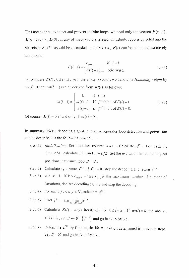
(3.21)

This means that, to detect and prevent infinite loops, we need only the vectors E(k -1),

E(k - 2), "', E(O) . If any of these vectors is zero, an infinite loop is detected and the

bit selection t<k) should be discarded. For 0 ~ 1< k, E(l) can be computed iteratively

as follows:

{

e (kl' if I = kE(l-1)= f

E(l) + e/k)' otherwise.

To compare E(l), 0 ~ I < k , with the all-zero vector, we denote its Hamming weight by

wt(l). Then, wt(l-1) can be derived from wt(l) as follows:

{

1,

wt(l-1) = wt(l) -1,

wt(l) + 1,

if 1= k

if /(I)th bit ofE(l) = 1

if /(I)th bit of E(l) = O.

(3.22)

Of course, E(l) = 0 if and only if wt(l) = 0 .

In summary, IWBF decoding algorithm that incorporates loop detection and prevention

can be described as the following procedure:

Step 1) Initialization: Set iteration counter k = 0 . Calculate z(O) . For each i ,

o~ i < M , calculate l; /2 and ui + li /2. Set the exclusion list containing bit

positions that cause loop B =0 .

Step 2) Calculate syndrome S(k) . If s(k) = 0, stop the decoding and return Z(k) .

Step 3) k ~ k +1. If k > klllax ' where kmax is the maximum number of number of

iterations, declare decoding failure and stop the decoding.

Step 4) For each .i, O..s; j < N, calculate rjJ~k) .

Step 5) Find /(k) = arg min rjJ(k).OSj<N ,jeB }

Step 6) Calculate E(l), wt(l) iteratively for 0 ~ 1< k. If wt(l) = 0 for any I ,

o~ 1< k, set B ~ B U{.f(k)} and go back to Step 5.

Step 7) Determine Z(k) by flipping the bit at position determined in previous steps.

Set B = 0 and go back to Step 2.

41

3.2.5 Iterative Decoding based on Belief Propagation or Sum-Product Algorithm

In 1996, LDPC codes were rediscovered [10]. To achieve near Shannon limit

performance, beliefpropagation (BP) [34] was used for decoding. The goal of the BP

decoder is to compute marginal a posteriori probability p(ci = 1/y,S) that code bit at

position i is 1, conditional on the set of the received symbols y and on the event S that

the transmitted digits satisfy the set of parity-checks given by the parity-check matrix

H. An algorithm for the computation of such marginal probabilities exists for belief

networks [34]. The algorithm is exact when the underlying graph has no cycles. When

applied to an LDPC code, the obtained marginal probabilities will not be exact due to

many cycles in the corresponding Tanner graph. Assuming that the errors introduced

due to the cycles are small, belief propagation was nevertheless applied [10]. This

assumption is reasonable, since as the size of the code increases, it becomes

increasingly easy to produce codes in which there are no cycles of length smaller than

or equal to a specified length.

Iterative decoding based on belief propagation (IDBP), commonly known as sum

product algorithm (SPA), is a symbol-by-symbol soft-in/soft-out decoding algorithm,

the same as maximum a posteriori (MAP) decoding [40]. It processes received symbols

iteratively to improve the reliability of each decoded symbol. The processing is based

on the parity-check matrix which specifies the code. After each iteration, we check

whether the stopping criterion is satisfied. If the stopping criterion is not satisfied, we

use the outputs of the previous iteration as inputs for the next iteration, and continue the

decoding iteration process. If the stopping criteria is satisfied, the decoding stops and

the hard decisions are made based on reliability values for each code bit.

Consider an LDPC code C of length N specified by a parity-check matrix H with

M rows and N columns. For each check sum, i.e. for each row i, 0:::; i < M , we define

the set N, of code bits that participate in the ith check sum as given in (3.10). For each

code bit, i.e. for each column j, 0:::; j < N, we define the set Mj

of parity-checks in

which thejth code bit participates as given in (3.11).

42

The algorithm associates quantities qi,; and r;,; with every non-zero entry in the parity

check matrix, and updates these quantities iteratively. It consists of two steps which are

repeated iteratively. They are called horizontal and vertical pass. Horizontal pass

updates quantities r"i' while vertical pass updates quantities qi,;' Initial values of qi,;

are determined by a posteriori probabilities at the channel output. For each nonzero

entry in the parity-check matrix, we have in fact, two qi,; quantities, q~;, and q:,i' but

they can be computed from one another and their sum is 1. The same is true for 'f,;'

In the lth iteration, quantity q/i represents the pseudo-posterior probability that the jth

code bit has value x given the information coming from code bits that are distance at

most 21 from corresponding variable node in the Tanner graph of a code, excluding

code bits that are connected to thejth code bit trough the ith check-sum,

The quantity r Xrepresents the probability that the ith check sum is satisfied given that1,./

the jth code bit has value x and that the other code bits participating in the check sum

have value x' , x' E {O, I} , with probability q/>, where j' E Ni and j' ~ j .

Initialization: Let p~ be the prior probability that code bit Vi is 0, and let P: = 1- p~ be

the prior probability that code bits Vi is 1. In the case of AWGN channel, these values

are P,O = P (v, = 0/y,) and p,l = P (v, = 1/Y, ) , i.e. probabilities that the transmitted code

bit at position i is ° and 1, respectively, conditional on the received value

corresponding to the ith bit. For every code bit at position j, O:s; j < N, we initialise

° 0 d I I ~ .Cfi.i=Pi an qi.j=Pi,loralllEMi .

Horizontal pass: In the horizontal step of the algorithm, we run through the parity

checks and for each parity-check, i,e. for each row i, and for each j EN,., we compute

two probabilities. One is the conditional probability that the ith check sum is satisfied,

gi ven that thejth transmitted bit is °and the other bi ts ill the set N, ,{c j' /.1' E N, ,.I' :t:- j} ,

43

have separable distribution given by the probabilities {q~/,q;,/} :

fj~i= L p(S/lc,=O,{c(!j'EN"j':;tj}) I1 q;/> ,h.Ij'EJ\(,./*i} j'ENj./*j

(3.23)

where S. denotes the event that the ith check sum is satisfied. The other probability isI

the conditional probability that the ith check sum is satisfied, given that the jth

transmitted bit is 1 and that the other bits in the set Ni have separable distribution:

r/ j = L P (Si Ici = 1, {cl' I j' E Ni' j' :;t j} ) I1 q/~>,{C··Ii'EN,j'*i} j'EN,'/*jI· I,·

(3.24)

These two probabilities can be efficiently computed if we consider Or . = 1'.0 - 1'.1.1,./ t •./ 1•./

instead of 'i~i and fj~i separately. Then we have the following equality:. .

Or . = TI Oq.."1,1 1.1i'EN,'/*j

(3.25)

where Oqi,j = q~j - q:,i . Once 01j,j is computed, r,°i and r,~i are computed as follows:

1'0 =~(1+0r )1,/ 2 1,./ '

1'1 =~(1-0r ).',1 2 1,1

(3.26)

(3.27)

Vertical pass: In the vertical step of the algorithm, we update q/~i and q,l,j based on

computed fj~i and fj~j in the previous step:

ql . = a .pl. I1 1'1/ './ I, I I i', i '

i'EM,.i'=1:i

where ai,j is a constant such that q~j + q:,i = I.

(3.28)

(3.29)

After the vertical step, we also compute the pseudo-posteriori probabilities for each

code bit j , with O:s j < N, given by:

P (c, =0 IY ) =ai p~ TI 1~~, '

iE/vt,

44

(3.30)

P (C i =1Iy ) =a i P~ IT r/ j ,

iEM j

(3.31)

where agam ai

IS chosen so that P (Cl =°Iy) + P (Cl = 11 y) =1 . Based on these

probabilities, we can form a vector z=(zo,zp""ZN_I) as candidate for the decoded

codeword:

z. ={l, forP(c i =1Iy»0.5J 0, otherwise.

(3.32)

From the determined candidate codeword z, z· HT is computed. If z· HT = 0, the

candidate codeword is indeed a codeword and the iterative decoding process is stopped.

Then z is given at the output of the decoder as the decoded codeword. If z· HT :j:. 0 , the

iterative decoding continues, i.e. we are going back to the horizontal pass with updated

values 5qj,j = q,~j - q;,j and we compute new values for 'i~i and 'i~j'

Iterative decoding based on belief propagation is computationally expenSIve. Each

decoding iteration requires many real number computations, If decoding of a particular

code with this algorithm converges slowly, a large number of iterations is required to

achieve the desire performance. This means that the number of computations is large as

well as the decoding delay. In the next section, two reduced complexity IDBP

algorithms [35] are given. Both are based on the fact that IDBP basically consists of

many maximum a posteriori (MAP) decoders for a single parity-check (SPC) code, one

corresponding to each parity-check sum, working in parallel. The MAP algorithm for

SPC codes and its approximation are described in Appendix A.

3.2.5.1 Reduced Complexity Iterative Decoding

IDBP for binary LDPC codes can be shown to be iterative parallel MAP-SPC decoding.

This allows us to apply existing approximations for MAP-SPC to IDBP and yields a

reduced complexity decoding algorithm.

Suppose we have M MAP-SPC decoders, one for each check sum of the parity-check

matrix H of an LDPC code, For each code bit at position .f , we can compute IMII

45

corresponding extrinsic log-likelihood ratios (LLRs), one for each check-sum that

contains thejth bit, where IMI I denotes the cardinaIity of the set M I , i.e. the number of

I-components in the jth column of the parity-check matrix. For every code bit at

position j , O:s j < N , and every check sum i E M; , let Li.; denote the LLR

corresponding to the jth bit that is used as input to the ith MAP-SPC decoder.

For each O:s j < N and each i E M I , initialize L i.; with the chalmel LLR for code bit at

position j, Le (Cl) = In (P (Cl = 11 Y I ) / P (Cl =0 IY I )) . Suppose that during the first step

of the iterative decoding, for O:s i < M , the output of the ith MAP-SPC decoder gives

the extrinsic LLR for every code bit j E Ni as follows:

(3.33)

Suppose that during the second step of the iterative decoding, for every code bit j ,

o:S j < N, and every check sum i E M I , Li .j is updated by adding to the channel LLR

Le(c,) extrinsic values at the output of all MAP-SPC decoders corresponding to check

sums containing thejth bit, except the output of the ith decoder:

L . = L (c) + ~ Lex.1•./ e / ~ 1•./

i'EMI,i'~i

(3.34)

It can be shown that the following relationships exist between 5q. . and L " 5r . and1•./ 1•./ 1,./

Lex.1./ .

!: anI ( I.,.})uql,; =t 1 -2 '

( 1"')51';,./ = tanh - '~I •

(3.35)

(3.36)

Using these relationships, it is straightforward to obtain equation (3.33) from (3.25), as

well as equation (3.34) from (3.28) and (3.29). Thus the above two step iterative

decoding is equivalent to IDBP. However, it is usually referred to as the sum-product

algorithm (SPA).

46

Based on the approximation for the MAP-SPC decoding given in Appendix A, we

obtain the following approximation of the horizontal step:

Lex::: (_l)IN;I. TI sign (Li ,.')', m.i~ {ILi".I}.1•.1 '. ,EN ,.",. .

j'EN,,J',,j . ".

(3.37)

If the channel is AWGN channel, and all the code bits are statistically independent with

the same probability of 0 and 1, we can replace P (Cl =x IYI ) with P (YI Icl =x) ,

N)2 is the noise variance. The term 4/ No can be factored out of all the equations.

Therefore, the algorithm does not depend on the noise variance, and is uniformly most

powerful (UMP). The algorithm is referred to as UMP BP-based iterative decoding

algorithm [35].

Additional approximation can be obtained if we modify the vertical pass as follows:

Li,} = LI = Le (x, )+ L L~~J for all i E M, .i'EM,

(3.38)

In this way, LLRs corresponding to bit j that are passed to the MAP decoders are the

same for every i EM.. This approximation leads to an algorithm called UMP a.I

posteriori probability (APP) based iterative decoding algorithm [35].

3.3 Two New Decoding Algorithms for Low-Density Parity-Check

Codes

In this section, two new decoding algorithms are presented. The first algorithm is a

hard-decision decoding method, and the second one is between hard- and soft-decision

decoding methods. For the sake of convenience and completeness, some notations and

definitions already introduced are repeated here.

47

3.3.1 Notation and Basic Definitions

A binary LDPC code is completely described by its sparse binary parity parity-check

matrix H. For an (N,K) LDPC code, H has N columns and M ~ N - K rows. For a

regular LDPC code, H has a constant column weight y and a constant row weight p.

Suppose a binary (N, K) LDPC code is used for error control over a binary-input

additive white Gaussian noise (BIAWGN) channel with zero mean and power spectral

density No /2. N is the code length and K the code dimension. Assume binary phase-

shift-keying (BPSK) signaling with unit energy. A codeword c = (co'cl' ... 'CN_1)

E {GF(2)t is mapped into bipolar sequence x = (xo,xp ... 'XN _1) before its transmission,

where x; =(2c;-I) with O~i~N-l. Let Y=(Yo,Yp ... ,YN - 1) be the soft-decision

received sequence at the output of the receiver matched filter. For 0 ~ i ~ N -1 ,

v = x + n where n is a Gaussian random variable with zero mean and variance N /2.""' I I I I ()

An initial binary hard decision of the received sequence, lO) = ( z6°) ,z;O) , ... , z~21 ), is

determined as follows:

(0) {I, if Y; ~ 0Z -i - .

0, if Y; < 0(3.39)

(3040)

For any tentative binary hard decision z made at the end of each decoding iteration, we

can compute the syndrome vector as s = z· HT . We define the log-likelihood ratio

(LLR) for each channel output Y;' 0 ~ i ~ N - 1 :

L ~ In P( C, = 11 y,)J P(c; = 0 IyJ .

The absolute value of L;, IL,I, is called the reliability of the initial decision 2;(0). For

any binary vector v = (vo' VI' ... ' V N _1), let wt(v) be the Hamming weight of v . Let u; be

the N-dimensional unit vector, i.e. a vector with "1" at the ith position and "0"

everywhere else.

48

3.3.2 Algorithm I

Step 1) Initialization: Set iteration counter k =° . Calculate z(O) and

S(O) = wt(z(O) . HT) .

Step 2) If S(k) = 0, then go to Step 7).

(k) (k-I) T )Step 3) k+.-k+1.Foreach i=O,1, ... ,N-1,calculate S, =wt (z +uJ·H .

Step 4) Find /k) E {O,l, .. .,N -1} with fk) = arg min S?).. 05,/<N

Step 5) If fk) = fk-1) , then go to Step 8).

Step 6)

Step 7)

Calculate Z(k) = Z(k-I) + U .(ll and S(k) = wt( Z(k) . HT) . Go to Step 2)..I

Stop the decoding and return z(k).

Step 8) Stop the decoding and return Z(k-I) .

So the algorithm flips only one bit at each iteration and the bit to be flipped is chosen

according to the fact that, on average, the weight of the syndrome increases with the

weight of the error. The criterion for the decision of whether or not a position is in error

differs from Gallager's algorithm because here the syndrome weights are compared

where the numbers of errors differ by two. Note that in some cases, the decoder can

choose a wrong position .f, and thus introduce a new error. But there is still a high

likelihood that this new error will be corrected in some later step of the decoding.

3.3.3 Algorithm 11

The above algorithm can be modified, with almost no increase in complexity, to achieve

better error perfonnance, by including some kind of reliability infonnation (or measure)

of the received symbols. Many algorithms for decoding linear block codes based on this

reliability measure have been devised.

Consider the soft-decision received sequence y = (Yo' Y1, .. . , YN-I)' For the AWGN

channel, a simple measure of the reliability, IL,I, of a received symbol Yi

is its

magnitude, IYI I· The larger the magnitude IYi I is, the larger the reliability of the hard-

49

decision digit Zi is. If the reliability of a received sYmbol Yi is high, we want to prevent

the decoding algorithm from flipping this symbol, because the probability of this

symbol being erroneous is less than the probability of this sYmbol being correct. This

can be achieved by appropriately increasing the values Si in the decoding algorithm.

The solution we propose is to increase the values of Si by the following term:

(3.41)

where a > °is some coefficient to be selected. This solution, which is very simple,

happens to be very efficient as will be shown by the simulation results in Section 4. Our

intuitive approach is justified by the following facts:

• A larger IL,I implies that the hard decision Zi is more reliable.

• If there is no overlap between the "non zero" elements of the different columns

of H , each additional column would increase the syndrome weight by y.

• For different values of the signal-to-noise ratio (SNR), the values of IL,I are not

the same. Hence the presence of the weighting factor.

The steps of the soft version of the decoding algorithm are described in detail below:

Step 1) Initialization: Set iteration counter k =° . Calculate z(O) and

S(O) = wt(z(O) . HT).

Step 2) If S(k) =°,then go to Step 7).

Step 3) k +-- k + 1. For each i = 0,1, ... , N -1, calculate

S,<"J = wt((Z(k-IJ +uJ.HT)+axyxILil.

Step 4) Find /k) E {O, 1, ... , N -I} with/ k) = arg min Si(k) .O<;i<N

Step 5) If /k) = /k-I) , then go to Step 8).

Step 6) Calculate Z(k) = z(k-1) + up} and S(k) = wt( Z(k) • HT). Go to Step 2).

Step 7) Stop the decoding and return z(k) .

Step 8) Stop the decoding and return Z(k-J) .

50

It is important to point out that, in both algorithms, the maximum number of iteration

needs not to be specified. The algorithms have an inherent stopping criterion. The

decoding stops either when a valid codeword is obtained (Step 2) or when the minimum

syndrome weight at the kth iteration and the minimum syndrome weight at the (!c-l)th

iteration are found in the same position (Step 5). This has also been verified through

simulations.

3.3.4 Loop Detection

Let fk) denote the bit position to be flipped at the kth iteration. It is clear that if

fk) = f k - I ) , then Z(k) = Z(k-2) and Z(k+u) = Z(k-2+o-) for any (J > O. The algorithm enters a

loop, and since a valid codeword was not found until the kth iteration, it will not be

found if the decoding continues. The loop can be detected and avoided by selecting the

bit to be flipped as the one that has the next smallest value of S?) , instead of selecting

the one with minimum S?) that would result in a loop. A loop detection technique is

introduced in [31] and described in the previous section. It can be applied to any search

algorithm. In the sequel, a somewhat easier implementation is presented.

Suppose that we are in the kth iteration, that positions of bits flipped so far are

fl), f 2), ... , f k

-I), and that the bit position selected for flipping at the !cth iteration is

fk) . For each position .i , 0:::; j < N, and for each !c' , 1:::;!c':::; le, we compute the

number, njk'), of times it appears in the set {fk'),/k'+'), ... ,fk

)} modulo 2. Next we

compute the weight of the binary sum Z(k'-I) + Z(k) , W(k'), as follows:

W(k') = "" n.(k')~ i .

O<;j<N

If VIP") = 0 for any !c' , that indicates the loop.

(3.42)

(k') (For 0:::; j < N , n· can be computed iteratively. Let n(k') = n(k') n(k') n(k'») we.I 0 , I , ... , N-I ,

have:

51

{

n(k'+I) +1 (mod 2) if j = ;lA')(A') _ .I " '

n· - "') ,I (k'+I) 'f' '(nn i ' I J::f:. )

(3.43)

for I::::; k' < k, with initial condition n;k) = 1 for j = fA) , and n;k) = 0 for j::f:. fA), We

can also compute w(k') iteratively as follows:

{

W(k'+I) + 1, ifW(k') =

W(k'+I) -1 if,

for 1 ::::; k' < k, with initial condition W(k) = I,

(k'+I) - 0n ,(k') -.I

(k'+I) -1 'n/ k·) -

(3.44)

In summary, Algorithm II described above that incorporates loop detection and

prevention is as follows:

Step 1) Initialization: Set iteration counter k = 0 , Calculate zeo) and

S(O) = wt(z(O) ,HT), Set the exclusion list containing bit positions that

cause loop B =0,

Step 2) If S(k) =0 , then go to Step 8),

Step 3) k ~ k +1, If k > kmax , where kmax is the maximum number of iterations, go

to Step 9),

Step 4) For each i = 0,1, .. " N -1, calculate S,Ck) = wt ((Z(k-I) + uJ· HT) + ay ILil,

St 5) F ' d '(k) {o I N I} 'th ,(k) 'S(k)ep m.l E " ' , . , - Wl .I = arg mm ' .O';i<NJ"B I

Step 6) Calculate 11(k') and W(k') iteratively for 1::::; k' ::::; k, If w(k') = 0 for any k' ,

set B U{f k)} and go back to Step 5),

Step 7) Calculate z(k) = Z(A-I) + u/kI and S(k) = wt ( z(k) ,HT) , Go to Step 2).

Step 8) Stop the decoding and return Z(k),

Step 9) Stop the decoding and return Z(k-I) ,

Tt is necessary to point out that when loop detection is used, the algorithm no longer has

an inherent stopping criterion. Thus the maximum number of iteration needs to be

specified,

52

3.3.5 Computational Complexity

Neglecting all operations associated with modulo-2 arithmetic as conventionally done,

the computational complexity of the second algorithm described above can be

calculated as follows. During each iteration, N -1 real comparisons are required to

select the bit to be flipped. After the bit is flipped, y x p operations are required to

update the syndrome. The terms axyxlL;1 need to be calculated only once before the

first iteration of the algorithm. Since comparison can be considered as additions, we

need altogether N -1 + Y x P real additions per iteration.

Loop detection, as described in the previous section, requires only bit operations and

integer counter increments/decrements. Most importantly, the total number of loop

detection operations is independent of the block length N and depends only on the

number of executed iterations. In practical applications, the user specified maximum

iteration number is much less than the block length N . Moreover, as the decoding

. converges, the average number of iterations is far less than the user specified maximum

iteration number. Therefore, the cost of loop detection in comparison with the

N -1 + Y x P real additions required by the core decoding procedure can be safely

ignored. The decoding complexity associated with the proposed algorithms and some of

the algorithms mentioned in Sections 3.1 and 3.2 are summarized in Table 3.1.

Table 3.1: Decoding Complexity per Iteration

Algorithm Multiplications Divisions Additions

IDBP algorithm 11Ny-9N N(y +1) N(3y +1)

Normalized BP-based 0 Ny 4N(y -1) + N log2 2y/2

UMP BP-based 0 0 4N(y -1) + N log2 2y/2

WBF 0 0 N-1+yxp

IWBF 0 0 N-1+yxp

Proposed algorithm II 0 0 N-1+yxp

53

3.4 Simulation Results

The elTor performance, in tem1S of bit-elTor rate (BER) as a function of the signal-to

noise ratio (SNR), of the algorithms presented in the previous section is compared with

some existing algorithms for different types of LDPC codes. The different codes studied

are given in Table 3.2. The following algorithms are simulated: MLG, BF (with

adaptive threshold), WBF, IWBF, IDBP, and the algorithms proposed herein. The

maximum number of iteration is set equal to 50 for IDBP, and 200 for the other

algorithms.

3.4.1 Performance of Algorithm I

Figures 3.1 and 3.2 show the performances of the (2048,1723) RS-LDPC code and the

(2048, 1664) PEG-LDPC code based on different hard-decision decoding algorithms. It

can be observed that, at the BER of 10-5, Algorithm I outperforms BF algorithm by

about 0.2 dB and 0.5 dB, respectively. It was observed through simulations of various

LDPC codes that Algorithm I always outperfonns BF algorithm, and that the

performance gap between the two algorithms decreases with column weight of the code.

For the Type-I 2-D (1023, 781) EG-LDPC code for example, the performance gap is

only about 0.1 dB at the BER of 10-5. As mentioned earlier, the criterion for the decision

if whether or not a position is in elTor differs from Gallager's algorithm in that here

syndrome weights are compared where the number of elTors differ by two. It IS

necessary to point out that Algorithm I is slightly more complex than BF decoding.

3.4.2 Impact of SNR on the Optimal Value of a in Algorithm II

For a given LDPC code with given column weight, at a given SNR, the performances of

Algorithm II vary with the value of the weighting factor a . The effect of a on the

BER performances of the (2048, 1664) PEG-LDPC code with column weight 3, the

(2048, 1664) PEG-LDPC code with column weight 6, and the (2048, 1723) RS-LDPC

code with column weight 6 are shown in Figures 3.3 - 3.5 respectively. It can be seen

that the optimal value of a decreases slowly as the SNR increases. It can also be

54

observed that at low SNRs, the perfonnance is not very sensitive to the value of a . The

same observations were made for the different LDPC codes studied.

3.4.3 Impact of Column Weight on the Optimal Value of a in Algorithm II

At a given SNR, or for a given BER, the optimal value of a in Algorithm II for

decoding different LDPC codes may vary with the corresponding column weights. The

optimal values of a at various SNRs for decoding different LDPC codes are given in

Table 3.3. It can be observed that the optimal value of a depends not only on the

column weight, but also on the structure of the code. For example, at a given SNR, or at

a given perfonnance level (BER), the optimal a for the RS-LDPC codes decreases

with the column weight, whereas it increases for the PEG-LDPC codes. On the other

hand, the optimal a is the same for both the (2048, 1723) RS-LDPC code and the

(2048,1664) PEG-LDPC code. The two codes have a column weight 6.

3.4.4 Impact of the Value of a on the Average Number of Iterations in

Algorithm II

Figure 3.6 depicts the effect of a on the average number of iterations for the decoding

of the (2048, 1664) PEG-LDPC code with parameters r =3, P =16. It can be seen that,

for any value of the SNR, the average number of iterations is at its lowest when a is

optimal. It can also be observed that at high SNRs, the average number of iterations is

not very sensitive to the value of a . The same observations were made for the different

LDPC codes studied.

3.4.5 Performance of Algorithm II With Optimal a

Simulation results of Algorithm II with optimal weighting factors (chosen as the

optimal a at BER of 10-5) for decoding various LDPC codes are shown in Figures 3.7 _

3.12. Also shown in these figures are the perfonnances those codes based on different

soft-decision decoding algorithms. It can be observed that, in all cases, Algorithm II

with loop detection (LD) offers a gain of about 0.1 dB over the IWBF, and is always

55

less than 0.6 dB away from IDBP. It can also be seen in Figures 3.7, 3.9, and 3.11 that,

at a BER of 10.5, the loop detection and prevention as described in the previous section

improves the performance of Algorithm II by about 0.3 dB and 0.4 dB respectively. The

same trends apply to other LDPC codes.

Table 3.2: Different LDPC codes simulated

Code type Length (N) Dimension (K) Rate Parameters

(EG)-LDPC code [22] 1023 781 0.763 r =32, p =32

2048 1723 0.841 r = 6, P = 32

2048 1649 0.805 r =8, p=32

(RS)- LDPC code [28] 2048 1605 0.784 r=10, p=32

2048 1561 0.762 r=12, p=32

2048 1664 0.813 r = 3, p = 16

PEG-LDPC code [50] 2048 1664 0.813 . r = 6, P = 32

56

1.E+OO

76.565.5

Eb/No (dB)

54.5

-+- Algorithm I

---+-- BF

~MLG

1. E-06

4

1.E-05

1.E-01

1.E-02

Q)

tu0::'-

1. E-03gw~

al

1.E-04


r = 6, p = 32 based on different hard-decision decoding algorithms.

57

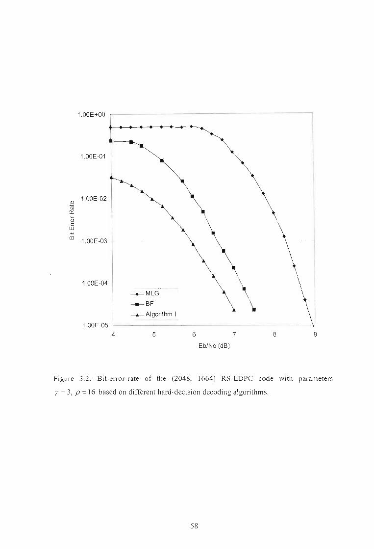
1.00E+OO

1.00E-01

1.00E-04

1.00E-02IDro

0:::....gw......CO

1.00E-03

1.00E-05

4

--+-MLG

---.- BF

--.- Algorithm I

5 6

Eb/No (dB)

7 8 9


r = 3, P = 16 based on different hard-decision decoding algorithms.

58

1.00E-01

1.00E-02

1.00E-03

<lJ 1.00E-04roIX:'-gw.... 1.00E-05co

1.00E-06

1.00E-07

~SNR = 2.5dB

_SNR = 3.5 dB

-+- SNR = 4.0 dB

-SNR = 4.5dB

-+--SNR =5.0 dB

----.-SNR = 3.0 dB

--+-- SNR = 3.75 dB '

~SNR = 4.25 dB,

---er-- SNR = 4.75 dB !

~SNR = 5.25 dB:

1.00E-08

0.2 0.4 0.6 0.8 1.2

Weighting factor

1.4 1.6 1.8 2


for the decoding of the (2048,1664) PEG-LDPC code with parameters r = 3, P = 16.

59

1.00E-01

1.00E-02

1.00E-03

a.> 1.00E-04ro0:::'-gw.....

1.00E-05co

1.00E-06

1.00E-07

_SNR = 2.5 dB

_SNR= 3.5dB

--SNR = 4.0 dB

~SNR= 4.5dB

----..-SNR = 3.0 dB

-+- SNR = 3.75 dB

--*- SNR = 4.25 dB

---A- SNR = 4.75 dB

1.9

1.00E-08

0.9 1.1 1.3 1.5 1.7

Weighting factor

Figure 3.4: Impact of the weighting factor a in Algorithm II on the BER perfonnance

for the decoding of the (2048, 1664) PEG-LDPC code with parameters r = 6, p = 32.

60

1.00E-01 ._-_.-._---_._--

1.00E-02 I--'&--~:t-----€.----e--_-e-_-e-_-&-__----f)

1.00E-03

Q) 1.00E-04ro0:::'-gw.....Cl) 1.00E-05

1.00E-06 ~.

1.00E-07

1.00E-08

--+-SNR = 2.0 dB

--?lE- SNR = 3.0 dB

-e-SNR = 3.75 dB

---4- SNR = 4.25 dB

---A--SNR = 4.75 dB

~

-.-SNR = 2.5 dB

-t-SNR = 3.5 dB

-SNR = 4.0 dB

-e--SNR =4.5 dB

1.2 1.4 1.6 1.8 2

Weighting factor


for the decoding of the (2048, 1723) RS-LDPC code with parameters r = 6, p = 32.

61

Table 3.3: Impact of Column Weight on the Optimal a in Algorithm II for Different

LDPC Codes.

Code type (N, K) WC SNR (dB) BER ao>,(EG)-LDPC code [11] (1023,781) 32 3.5 1.9x10-3 1.1

3.75 2.3xlO-4 1.0

4.0 lAx lO-s 0.9

4.125 3.0xlO-6 0.9

(RS)- LDPC code [22] (2048, 1723) 6 4.0 1.3x1003

1.8

4.25 1.4x10=4 1.6

4.5 1.6xlOos lA

4.75 1.1 X 1006

1.2

(2048, 1649) 8 3.75 4.1xlO03

1.5

4.0 7.1xl0:4 1.5

4.25 5.6xlOo) 1.3

4.5 3.9x10-6 1.2

(2048, 1605) 10 3.75 3.3xlO-3 1.5

4.0 5.3xlO-4 lA

4.25 2.9xlOo) 1.2

4.5 4Ax 10=7 1.2

(2048, 1561) 12 3.75 3.2x1003

1.6

4.0 4.0xlO-4 lA4.25 2.8xlO-s 1.2

4.5 1.3x10061.2

PEG-LDPC code [23] (2048, 1664) 3 4.0 1.5xlO-3 lA4.5 1.5xl0-4 1.3

5.0 1.2x lOoS 1.2

5.25 2.8xl0001.1

(2048, 1664) 6 4.0 3.2x 10-3 1.7

4.25 6.0x 10-4 1.6

4.5 5.2xlOoo lA4.75 4.0x 10-0 1.2

62

200

180

160

140

IIJc0 120~~'+-

1000'-ill.nE:::J 80 - - --

Zillenro'-

60ill>«

o_SNR = 3.5 dB~SNR = 4.0 dB-e-SNR = 4.5 dB-er- SNR =5.0 dB

-.-SNR = 3.75 dB~ SNR = 4.25 dB---+-SNR = 4.75 dB- SNR = 5.25 dB

-20

0.2 0.4 0.6 0.8 1.2 1.4 1.6 1.8 2

Weighting factor

Figure 3.6: Impact of the weighting factor a in Algorithm II on the average number of

iterations of the (2048, 1664) PEG-LDPC code with parameters r = 3, P = 16.

63

---- ------

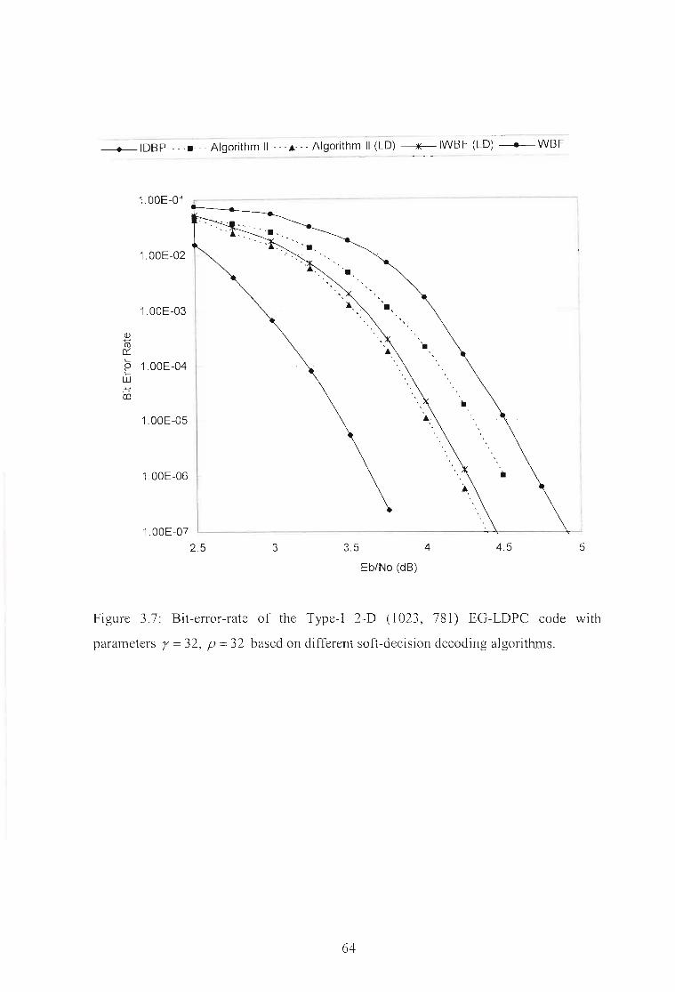
-----+-IDBP . --.--. Algorith~-II -- -.&-- - Algorithm 11 (LD)~ IWBF (LD) • WBF

54.543.53

1.00E-07

2.5

1.00E-06

1.00E-01

1.00E-02

,

1.00E-03

Q)

ma:...

1.00E-04e...w......en

1.00E-05

Eb/No (dB)

Figure 3.7: Bit-error-rate of the Type-I 2-D (1023, 781) EG-LDPC code with

parameters r =32, P =32 based on different soft-decision decoding algorithms.

64

! -+-IDBP - - -~- - - Algorithm 11 (LD) ---..-IWBF (LD) --WBF '

1.00E-01

1.00E-02

Q) 1.00E-03con::....gw~

co 1.00E-04

1.00E-05

1.00E-06

2.5 3 3.5 4 4.5 5 5.5 6

Eb/No (dB)


r = 6, P = 32 based on different soft-decision decoding algorithms.

65

1.00E-01

1.00E-02

1.00E-03QJ

m0:::'-0'-'-w.....co

1.00E-04

1.00E-05

1.00E-06

2

--+--WBF___ IWBF (LD)

- - -~- - - Algorithm 11 (LD)

----*-IDBP

- - - /::,- - - Algorithm 11

3 4

Eb/No (dB)

5 6


r = 8, p = 32 based on different soft-decision decoding algorithms.

66

1.00E-01

• WBF

______ IWBF (LD)

- - -~- - - Algorithm 11 (LD)

)( IDBP

1.00E-02

Q)1.00E-03ro

0::'-0l.:::UJ.....CO

1.00E-04

1.00E-05

1.00E-06

2 2.5 3 3.5 4

Eb/No (dB)

4.5 5 5.5 6

Figure 3.10: Bit-error-rate of the (2048,1605) RS-LDPC code with parameters


67

1.00E-01

1.00E-02

1.00E-03

Q)

ro0::

L...gw 1.00E-04

1.00E-05

1.00E-06

1.00E-07

2

... WBF

___ IWBF (LD)

- - -)1(- - • Algorithm 11 (LD) ,

-----*- lOBP

- . - /:;... Algorithm 11

3 4

Eb/No (dB)

5 6

Figure 3.11: Bit-enor-rate of the (2048, 1664) PEG-LDPC code with parameters


68

3.5 Conclusions

In this Chapter, two new decoding algorithms for LDPC codes are presented. The first

algorithm is a hard-decision method, and the second one is a modification of the first to

include reliability information of the received symbols. In principle and in complexity,

the algorithms belong to the class of bit flipping algorithms. The defining attribute of

the proposed algorithms is the bit selection criterion which is based on the fact that, for

low-density matrices, the syndrome weight increases with the number of errors in

average until error weights much larger than half the minimum distance. A loop

detection procedure with minimal computational overhead is also proposed that protects

the decoding from falling into infinite loop traps. Simulation results show that the

proposed algorithms offer an appealing performance/cost trade-offs and may deserve a

place in an LDPC decoding "toolbox". One drawback of the soft version of the

algorithm is that the optimal weighting factor a is SNR-dependent and code

dependent. However, choosing the optimal a at BER 10-5 and keeping it constant at

any SNR does not cause significant degradation in performance. Therefore, the optimal

weighting factor a can be considered to be only code-dependent

Some modifications can easily be applied to the decoding algorithms to increase the

decoding speed. For example, one can flip more than one bit in each iteration. As

another example, the computation of the syndromes in Step 4) can be done only for the

bit positions whose reliabilities are below a certain threshold.

69

CHAPTER 4

GENERALAZATION OF IRREGULAR LOW-DENSITY

PARITY-CHECK CODES

In this chapter, a new class of codes called generalized irregular low density (GILD)

codes is presented. This family of pseudo-random error correcting codes is built as the

intersection of randomly permuted binary codes. It is a direct generalization of irregular

LDPC codes (see Chapter 2), and is adapted from the previously known class of

generalized low density (GLD) codes introduced independently by Lentmaier et al.[55],

and Boutros et al. [56] [57].

It is proved by an ensemble performance argument that these codes exist and are

asymptotically good in the sense of the minimum distance criterion, i.e. the minimum

distance grows linearly with the block length. Upper and lower bounds on their

minimum Hamming distance are provided, together with their maximum likelihood

decoding error probability.

Two iterative soft-input soft-output (SISO) decoding for any GILD code are presented,

and iterative decoding of GILD codes for communication over an AWGN channel with

binary antipodal modulation (BPSK) is studied. The results are compared in terms of

perfonnance and complexity with those of GLD codes. The high flexibility in selecting

the parameters of GILD codes and their better performance and higher rate make them

more attractive than GLD codes and hence suitable for small and large block length

forward error correcting schemes. Comparison between simulation results of a GILD

code and the best LDPC code of length 1008 and rate 0.5 shows very close

performances, suggesting that variations of GILD codes may be able to match or beat

LDPC codes for small block lengths.

70

This chapter is organised as follows: in the next section an introduction is presented.

The construction of GILD codes is described in Section 4.2. The ensemble performance

of these codes is studied in Section 4.3. It is shown that GILD codes are asymptotically

good and lower bound on their minimum Hamming distance is provided. In Section 4.4,

average upper bounds on the minimum Hamming distance of GILD codes of fixed

length and constituent code are calculated semi-analytically. In Section 4.5, average

bounds for the bit error probability when maximum likelihood decoding is used are

presented. The decoding algorithms are presented in Section 4.6. Simulation results are

presented in Section 4.7 and, finally, conclusions are drawn in Section 4.8.

4.1 Introduction

As a direct generalization of Gallager's LDPC codes, Generalized Low-Density (GLD)

Parity-Check codes were recently introduced by Lentmaier [55] and Boutros [56],

independently. GLD codes are constructed by replacing each single parity check in

Gallager's LDPC codes with the parity check matrix of a small linear block code called

the constituent code. It has been shown that GLD codes are asymptotically good in the

sense of minimum distance and exhibit an excellent performance over both AWGN and

Rayleigh channels [55], [56], [66]. Moreover, Pothier [66] demonstrates that GLD

codes can be considered as a generalization of product codes, and because of their

higher flexibility on the selection of code length, GLD codes turn out to be a promising

alternative to product codes in many applications like digital audio and TV

broadcasting, high speed packet data transmission and deep space applications.

As originally suggested by Tmmer [8], LDPC codes are well represented by bipartite

graphs in which one set of nodes, the variable nodes, corresponds to elements of the

codeword and the other set of nodes, the check nodes, corresponds to the set of parity

check constraints which define the code. Regular LDPC codes are those for which all

nodes of the same type have the same degree. This means that the parity-check matrix

of the code contains the same number of ones in each row and the same number of ones

in each column. Irregular LDPC codes, introduced in [61], [67], and further studied in

[16], [17], [18], [19J, [20], were demonstrated in [18] to substantially outperform

71

similar codes based on regular graphs. For such an irregular LDPC code, the degrees of

the nodes on each side of the graph can vary widely. In terms of the parity-check matrix,

the weight per row and column is not uniform, but instead is governed by an

appropriately chosen distribution of weights. Actually, GLD codes can be considered as

a generalization of regular LDPC codes.

Inspired by these recent results showing that irregular structure improves perfonnance,

the generalization of irregular LDPC codes is introduced, where small linear block

codes are used as component codes instead of single-error detecting parity-check codes.

4.2 Definition and Construction of GILD Codes

It has been shown that binary GLD codes with only J = 2 levels are asymptotically good

[55], [56], [66] (A more detailed description of GLD codes can be found in those

references). Furthermore, GLD codes with only 2 levels have the highest code rate and

simple decoder structure. Thus in this work, only GILD codes_ with two levels are

considered. However, the construction method presented here can be easily applied to

GILD codes with more than two levels.

4.2.1 Definition

A binary GILD code with two levels is defined by three parameters:

• The length of the code N.

• The length n of the component code Co, with dimension k and rate r.

• The fraction, B(B < 1), of the code symbols connected to the second super-code.

It should be noted that both Nand BN must be multiples of n.

4.2.2 Construction

To construct the parity-check matrix H of such a code, a low-density (LD) matrix with

N-;(l+e) rows and N columns, having exactly BN columns with 2 ones, N(l-e)

72

columns with lone, n ones in each row, and zeros elsewhere is first constructed. Then,

in each row of this matrix, the N-n zero elements are replaced by a zero column-vector

of length (n-k), and the nonzero elements by one of the n different columns of the

component code's parity-check matrix, each used once. It is important to note that if

Hamming codes or BCH codes are used as constituent codes, the parity-check matrix of

the resulting GILD code is not low density and may contain many short cycles. This is

because the conventional parity-check matrices of Hamming codes and BCH codes are

not low-density and their Tanner graphs usually contain many short cycles.

The construction of the LD matrix can easily be achieved using a technique similar to

that of [2]. This matrix is divided into 2 submatrices. The first of these submatrices

contains all its l's in descending order; that is, the i th row contains 1's in columns

(i -l)k +1 to ik . The second submatrix is not just merely a permutation of the first, but

a column permutation of the first over a selected number of rows. The permutation is

perfol111ed such that no two parity-check sets would contain more than one digit in

common, i.e. the resulting LD matrix is free of cycle of length 4 in its Tanner graph.

This, in effect, ensures that two constituent codes in the resulting GILD code have not

more than one digit in common. Figure 4.1 shows an example of a LD matrix for a

GILD code of length N = 20, n = 4, and 8 = 0.8. Note that, unlike the interleaver in

regular LDPC codes and GLD codes, re here is an "irregular" interleaver acting only on

a selected number ofrows of the first submatrix, 4 out 5 in this example.

The parity-check matrix H of the GILD code with two levels can be divided into two

submatrices, HI and H 2. HI is a block diagonal matrix and produces the direct sum of

N / n constituent codes, where N is the GILD code length. The second submatrix is

constructed as: H 2= re(H I), where re represents a random column permutation over

(eN/n) rows of HI. A (N, n, B) GILD code C can be considered as the intersection of 2

super-codes Cl and C2

, whose parity check matrices are the two submatrices, HI and

H2

, respectively. If the parity-check matrix H has full rank, the total rate of the GILD

code is:

R=(l+e)r-e.

73

(4.1)

.........>............N.=.2.O' .<.n=4< >

111 1 000 0 0 0 0 0 0 0 0 0 0 0 0 0o 0 0 0 1 1 1 1 000 0 0 0 0 0 0 0 0 0o 0 0 0 0 000 1 1 1 1 0 0 0 0 0 0 0 000000 0 0 0 0 0 001 1 1 100 0 0o 0 0 0 0 0 0 0 0 0 0 0 0 0 0 0 1 1 1 1

100010001 000 1 0 0 0 0 0 0 000000 1 000 1 000 1 001 000001 0 0 0 0 0 0 0 1 000 1 001 0 0000 1 000 1 000 0 0 0 0 1 000 1

Figure 4.1: Example of a low-density matrix of a GILD code for N = 20, n = 4, and

e= 0.8.

In case of smaller rank, the rate is increased accordingly. However, with increasing

block length N, (4.1) gives a good approximation of the actual rate of the code. Note

that the rate of the corresponding GLD code would be:

R' = 2r-1. (4.2)

Clearly R > R' since e< 1. This is the first advantage of GILD codes over GLD codes.

Flexibility in defining the code rate to suit particular applications can be achieved by

changing the value of e. It should be noted that if 8 = 1, we obtain a GLD code.

4.3 Ensemble Performance

In this section, the average weight distribution of GILD codes over all possible

interleavers as a function of the component code Co, and the length N is studied. From

this distribution, an asymptotical upper bound that allows us to prove that GILD codes

are asymptotically good is deduced and their minimum distance is compared with the

Gilbert-Varshamov (GV) bound. The maximum transition probability of the BSC

74

channel that an asymptotical GILD code with fixed rate can achieve with maximum

likelihood decoding is also derived and is compared to the BSC capacity7.

4.3.1 Average Weight Distribution of GILD Codes

The direct computation of the exact weight distribution of GILD code becomes rapidly

intractable when N increases. However, the weight distributions of the constituent codes

used in practical GILD codes (Hamming codes, extended Hamming codes, BCH codes

with error correction capacity t = 2 and extended BCH codes) are well known. See [23]

(p. 142) for Hamming and extended Hamming codes, [68] (p. 451 & p.669), and [69]

(Ch. 16) for the family of BCH codes. The average weight coefficient of a GILD code

can be easily obtained by averaging over all the possible interleavers Tr .

Let us denote by g(s) the moment generating function of the component code, which is

the exponential polynomial whose coefficient gi of degree i is the normalized number

of codewords with weight i. For example, the moment generating function of the (7, 4,

3) Hamming code is:

()1+7e3s+7e4s+e7s

g s =------16

(4.3)

The first super-code, Cl, is the direct sum of N /11 independent constituent codes Co .

Hence, its moment generating function GI (s) is simply a power ofg(s):

G1 (S)=g(st/1I

= LQ(!)e'S,

I

(4.4)

where Q(z) is the probability that a codeword of Cl has weight I. Since the total number

f d d · Cl. (2 k )N/II Io co ewor s m IS , the number of codewords of C having weight 1is:

(4.5)

7 The analyses in this section are similar to those in [56] concerning GLD codes.

75

The second super-code, C2, however, is the sum of eN/n independent constituent codes

Co and a code of length N(l- e) generated by the all zero matrix. Thus its moment

generating function is:

(4.6)

where K(l) is the probability that a codeword in C2 has a weight I. Since the total

number of codewords in C is (2 k YBN/I1) 2N(I-B), the number of codewords of C2 having

weight 1is:

N2(I) =2N(Bk/Il+(H1)) K (I) . (4.7)

Due to the fact that Cl and C2 are totally independent, the probability, P(l), that a vector

of weight 1belongs to C = Cl nC 2 is the product of the probabilities that it belongs to

each super-code, that is:

Finally, the average number of codewords in C having weight 1is:

N[(I+B)~+( I-B)]

N(t)~(nXP(I)~ 2 (;f')K(t)

(4.8)

(4.9)

This formula is the starting point of different analytical or semi-analytical results

presented in the following sections.

76

1.00E+120

1.00E+110,

1.00E+100I

II

1.00E+90\

1.00E+80 IUJ'0I- 1.00E+700~Q)'0 1.00E+600u

'+-0 1.00E+50l-Q).0E 1.00E+40:::lc

1.00E+30

1.00E+20

--GILD1.00E+10

1.00E+00 ... - - - . Binomial

: approximation i1.00E-10

---'---

0 200 400 600 800 1000

code\NOrd \Neight

Figure 4.2: Average weight distribution of a GILD code of length N = 961, () = 0.903

based on the (31, 21, 5) BCH code, compared with the binomial approximation.

4.3.2 Lower Bound on the Asymptotic Minimum Distance

The following theorem gives an upper bound for the average number of codewords of

weight I, NU) .

Theorem 4. J: Let C be a binary GILD code of length N built from a linear (n,k) block

code Co' Let NU) be the average number of codewords of weight 1 in C averaged over

all the possible interleavers 1[. Then for I> 0, NU) is upper bounded by:

N(l) ~ C(..1-, N) x e-NB(A.s) , (4.10)

77

where A = !IN is the normalized weight. The two functions C(A, N) and B(A, s) are

expressed as follows:

and

C(A,N)=~2JrNA(I-A)exp( ~ )],12NA I-A

(4.11)

B(A,S) = H (A)+ 2AS - (1 + B) (,u( s) + k log2) -(I-B)log(1 +eS), (4.12)

n

where H(A) is the natural entropy function and ,u(s) = log(g(s)).

Proof By using exactly the same bounding technique as Gallager [1, pp. 13-17], i.e.

upper bounding roughly each coefficient Q(l) in (4.4) by the entire function G1(s) and

each coefficient K(l) in (4.6) by the entire functionG2 (s), we obtain:

(4.13)

and

(4.14)

Defining ,u(s) = In(g(s)) and the normalized weight A = !IN, (4.13) and (4.14) can be

rewritten respectively as:

(4.15)

(4.17)

and

Let us now lower-bound the denominator in (4.9), which is the binomial coefficient.

Extended Stirling bounds on z! are [70]:

-J2Jr.zz=e-= ~ z! ~ -J2Jr.z z=e-: exp ( 1~z ) ,

and give for the binomial coefficient:

eXP{NH(Al- 12N(\_Al} ~(NJ=(N J< exp{NH(A)}

~2JrNA(I-A) ! AN - J2JrNA(I-A) ,

where H(A) is the natural entropy function:

78

(4.18)

H (1 ) =-1 In (1 ) - (1 - 1) In (I - 1) . (4.19)

Introducing (4.14), (4.15), and (4.18) gives:

N(l)~ !2JrN1(1-1)exp { ~ )}\j 12N1 1-1

. (4.20)

xexp { -N[H(A)+ Hs- (1 :0) (.u(s)+ kln2)-(l-O)ln(l +e')]}

We define:

and

C(1,N)=~2JrN1(1-1)exp( ~ )],12N1 1-1

(4.21 )

(4.23)

B(1,s) = H(1)+ 21s- (1 +8) (p(s)+ k log2)-(1-8)log(1 +es). (4.22)

n

Asymptotically, when the length N tends to infinity, N(l) tends to zero if B(1, s) is

strictly positive. For a given value of 8, our aim is now to find (if it exists) the largest

value 5 of 1 satisfying B(5, s) = 0 and B(1,s) < 0 for 1> 5. This value of 5 would

give us an asymptotical lower bound on the normalized minimum distance of the GILD

code.

B(1, s) is a function of an arbitrary parameter s we have to optimize in order to get the

tightest bound, namely we want B(1, s) as large as possible for each 1. Let us denote

by fA (s) the part of B(1, s) that depends on s:

fA(s)=21s- (1+8) p(s)-(l-8)ln(l+e').n

Finding the value of s that maximizes B(1, s) is equivalent to finding the value that

maximizes fA (s). When we set the derivatives of fA (s) equal to zero, we get:

1 _ (1 + 8) '(.) (1- 8) eS

ofll - I-t .s + .2n 2 1+ eS

79

(4.24)

We do not try to invert this relation. A large range of values of s will be covered, and

(4.24) will give us the value A0

/11 of A for which B(A, s) is optimal. Before doing this,

we have to make sure that (4.24) is one-to-one in order to cover the whole range of

values assumed by A between °and 1/2 and that fA (s) is a convex nfunction of s.

As g(s) is the moment generating function ofthe constituent code, it can be written as:

" . 1" .g(s) = Ig,e

lS= -kI vvie

lS,

i~O 2 i~O

where w, is the number of codewords of Co of weight i. We have:

and

( J( J ( J?

11 11 " -

I i2gieiS I gieiS - I igieiS

;.l'(s) = I~O I~() ? ,~O

(Ig,e'"'J-,~()

where, for each 1E [0, .. " 2n], Ut equals:

I t

Ut =Ilgjgt-j - Ij(l- j)gjgt-jj~O j~()

t

= Igjgt-)(2j -I)j~O

ltJ= I gjgt_jj(2j -I) + (1- j)(I- 2j)

j~O

ltJ=Igjg,_/2j _/)2 .

j~()

80

(4.25)

(4.26)

(4.27)

(4.28)

This proves that each Ut is non-negative, and so is /"/'(s) for all s. Thus, ,.1,01'1 as defined

by (4.24) is a monotonic increasing function of s. We have:

A = (1 + B) " (s) + (1- B) eS

op' 2n J 2 1+ eS

1/

"'" . isL}e(1 + B) ;;\ g, + (1- B) e

1/ 2 1 s'2n "",. is + eL.zg;e;;\

hm ADP' = 0,s~-oo

\im A 1 = 1.S--7+O:> 01'

Figure 4.3 shows Aop,(s) for a specific constituent code.

Let us now show that fA. (s) is a convex nfunction ofs. We have:

/1/(s)=_(I+B) p"(s)-(1-B) eS

?

A. n (1 + eS)-

(4.29)

(4.30)

(4.31)

Hence, f;'(s) is non-positive, and f;(s) is a monotonic increasing function, which is

negative for all values of s such that (1 + B) p'(s) + (1- B) eS

< A, and positive for all2n 2 1+ eS

(1 +B), (1 - B) eS

values of s such that Jt (s) + > A. Consequently, fA. (s) and B(A, s)2n 2 1+ eS

are convex n function ofs, with their maximum value satisfying (4.24).

The behaviour of B ( AOtJ/' s) for a GILD code based on a specific constituent code is

shown in Figure 4.4. The highest value of A such that B(A s) > 0 gives us theopt opt'

average normalized Hamming distance 0 . Hence the asymptotic lower bound on the

minimum distance of GILD codes can now be calculated as follows:

1. Start with positive value ofs.

2. Calculate ADP' using to (4.24).

3. Calculate B ,(s)=B(A ,s).op opt

81

4. If BoP/(s) < 0, decrease the value of S and return to 2, else cS = ADP/ is an

asymptotical lower bound on the normalized minimum distance of the GILD

code.

_.._-_..__...._--_...._-----_.._--------_.._------_._... _._..-._---_._-_.__._.::;--=--------,

i0.9

0.8

0.7a.0 0.6ro-0E~ 0.54-0If)

<lJ 0.4:::l

ro>

0.3

0.2

0.1

0-5 -4 -3 -2 -1 0 2 3 4 5

values of s

Figure 4.3: AoP/(s) for a GILD code based on the (31, 21,5) BCH component code. e =

0.903.

82

0.02

0.015

----ro"'0E 0.01ro::::..CDc0:p 0.005<.)c::l

'+-......cQ)c 000.XQ)

-0.005

______________ ---~--------- -- .----------- ----- - - ---- - ------ - . -------,··-----1

-0.01

o 0.025 0.05 0.075 0.1

normalized weight lamda

Figure 4.4: B (Ao",' s) plotted as a function of AOP1

for the GILD code based on the (31,

21,5) BCH component code. e = 0.903.

Table 4.1 shows the values of 5 found for some constituent codes and different values

of e. The Gilbert-Varshamov bound given by 50 =H;I(I-R) is also shown. All the

values found are strictly positive, which means that GILD codes are asymptotically

good for the corresponding values of e. It can be seen that the asymptoticallower bound

on the normalized minimum distance of the GILD code decreases as the values of edecrease. Also shown in Table 4.1 is, for each constituent code, the value of e for which

we could not find a value of IL satisfying B(IL, s) > O. For this value of e and all the

values below it, the corresponding GILD code is not asymptotically good.

83


of some GILD Codes compared with the Gilbert-Varshamov bound 60 , * indicates that

6 does not exist.

Constituent Code Co Value ofe Rate of the GILD Code 6 50

1 0.143 0.187 0.281

Hamming 0.95 0.164 0.144 0.266

(7,4,3) 0.9 0.186 0.091 0.252

0.875 0.196 * 0.245

1 0.467 0.026 0.121

Hamming 0.975 0.473 0.018 0.119

(15, 11,3) 0.95 0.48 * 0.117

1 0.355 0.116 0.164

0.95 0.371 0.099 0.158

BCH (t=2) 0.9 0.387 0.080 0.151

(31,21,5) 0.85 0.403 0.053 0.145

0.825 0.411 * 0.142

1 0.313 0.143 0.183

0.95 0.330 0.126 0.175

Extended BCH 0.9 0.347 0.107 0.168

(32,21,6) 0.85 0.364 0.083 0.161

0.825 0.373 0.066 0.157

0.8 0.381 * 0.154

1 0.619 0.031 0.074

BCH (t=2) 0.95 0.629 0.021 0.071

(63,51,5) 0.925 0.633 0.015 0.070

0.9 0.638 * 0.069

1 0.594 0.038 0.081

Extended BCH 0.95 0.604 0.029 0.078

(64, 51,6) 0.925 0.609 0.022 0.077

0.9 0.614 * 0.075

84

4.3.3 BSC Channel Threshold

In this section, communication over a BSC channel with transition probability p is

considered, and the maximum value ofp for which the word error probability Pew of an

ML decoder goes to zero when N is large is computed. The following theorem gives an

upper bound for the asymptotic average error probability of ML decoding of GILD

codes over a BSC channel with transition probability p.

Theorem 4.2: Assume a GILD code C of length Nbuilt from a linear (n,k) block code

Co is used on a BSC with crossover probability p, and let the codewords be used with

equal probability. Then the asymptotic average error probability of ML decoding of C is

upper bounded by:

where

_ 1

~: ~ LD(N,A,p,c)exp(-NE(A,S,p)),A.~O

(4.32)

A (I-A) [1 JD N, A S = NcC A N - ex( . , ,p) ( , ) 2 2JrN(p-A/2)(1- p-Aj2) P 12N(1-A) , (4.33)

and

E(A,S,p) = B(A,S)+ H(p)- A log2 -(1- A)H( P- A/2).1- A

(4.34)

Proof As a first step, we will derive an upper bound of Pew for any value of N,

depending only on the weight distribution N(l) of the GILD code. In a second step, we

will use the result (4.10) on the asymptotic average weight distribution of GILD codes

to compute ~:, the asymptotic average error probability of ML decoding of GILD

codes, and compare it with the BSC capacity.

Let us assume that the all-zero word 0 of a linear binary block code C of length N is

transmitted over the BSC chatmel. Let E be the ensemble of all possible error vectors,

that is:

(4.35)

85

where V o is the Voronoi region of O. Let us partition E with respect to the Hamming

N

weight of its vectors E = UEi as:1=1

E, = {~E E/w(~) = i}

= {~E GF(2t /w(~) = i and 3f:t= 0EC/dH (~,d:s dH (~,O)}, (4.36)

where w( ) is the Hamming weight of a vector and d H (,) is the Hamming distance of

two vectors. We have:

N N N

~II' = LP(d =L L p(d =L L pi (1- pt- I=LIEilpi (1- pt- I

• (4.37)~El": ;=1 ~EJ:;i ;=1 ~EJ::, 1=1

Let us denote by Ei (fi ) the set of error vectors of weight i that lead to the decoding of

the codeword f i of weight j:

(4.38)

~ 11 1 I 0 0 I

~ 2.£; 11.. .. ·· .. ·.. ·.. ····· .. ··· ···· .. 1 I 0 0 I

J

Figure 4.5: Error vector ~ and codeword f i . The Is of each vector are drawn at the first

positions of the vectors to help understanding.

Let us denote by 1 the number of 1s that an element ~ of El (fi

) has in common with f1

(see Figure 4.5). Hence, ~ has i -I ones where f i has zeros. The Hamming distance

between e and c. is:- -,/

dH (~, ft·) = .i -I + i -/ = i + .i - 2/ .

86

(4.39)

Equation (4.38) leads to the following inequality for I:

Ii-l :s; 1 :s; min(i, j) . (4.40)

That means that an error occurs when at least half of the I-bits of a codeword are

covered by an error vector. The same argument is used on the ensemble of the linear

binary block codes to derive the random-coding upper bound on the error probability in

[23] pp. 92-99. Hence the cardinality of E; (fi ) equals:

(4.41 )

Let us denote by E . the set of error vectors of weight i that lead to the decoding of aI.)

codeword of weight j. There are N(j) such codewords. Because an error vector ~ of

Ei. i can be closer to two or more codewords of weight .f than the all-zero codeword, we

have the following inequality:

We then have:

and:

IE;I:s;. f N(j)11lIj)(.fJ( ~-.fJ,

.=d . _r ill 1-II !!mlll I-I I

p :s;~ i(l_ )N-I ~ N( .)11l~j)(jJ(N-.fJ .ell' L.P P L. .J L. 1 . 1

i=l j=d"lIlill /=rt1 I -

(4.42)

(4.43)

(4.44)

Note that the bounding occurs in and only in (4.42). The last inequality can be used to

compute the ML decoding word error probability of any linear code of which we know

the weight distribution. It is tighter than the conventional union bound on the error

vectors weight combined with the Chernoff-Bhattacharrya bound on the pairwise error

probability ([71] p. 63):

N I

~"':s; I N(l)~4p(l- p) .

87

(4.45)

We are interested in the maximum crossover probability p of the BSC that leads to an

asymptotically vanishing word error probability p,,: in (4.44) when N tends to infinity.

In (4.37), we have to focus our attention on the term that occurs with the highest

probability. Intuitively, when N grows, the weight J of the error vectors tends to pN .

First, compute the probability that the normalized error weight () = i/N is:

p-E5,()5,P+E, (4.46)

(4.47)

where E is an arbitrary nonnegative value. It is closely related to the Chemoffbound on

the tails of a binomial distribution. If 7J is a random variable with finite moments of all

order and pdf p(7J} we have:

P b( > }<E( "('1- r))= r(s)-srro 7J-T _ e e ,

where s is any non-negative value and ['(s) = In L eS'I p(7J}. Minimizing (4.47) on s'I

results in:

P ob( > }<E( s('1- r ))= r(s)-.,f'(s)r 7J-T _ e e , (4.48)

where T = ['. (s) = d1(s}. We apply this equality to the weight of an error vector ofds

length N. We define

N

7J=w(d= Le",,,=1

(4.49)

where ell are the iid components of the error vector §!. and take the value 0 with

probability 1- p and 1 with probability p. Equality (4.48) can be rewritten in this case:

Prob(77 ~ i) = Prob(ry ~ ()N):S; eN[r(I)-lr'(')]

where

() l(s) I ~ "ey S =N = n L"e "p(eJ =In(1- p + pe').

e"

The optimal value of () is:

S

()=y'(s)= pe ,1- p+ pes

and leads to:

88

(4.50)

(4.51)

(4.52)

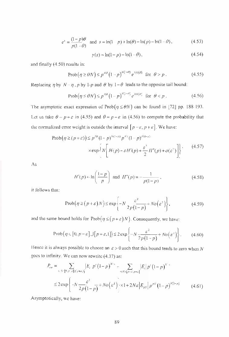
eS = (l-p)B and s=ln(l-p)+ln(B)-ln(p)-ln(l-B), (4.53)p(l-B)

y(s)=ln(l-p)-ln(l-B), (4.54)

and finally (4.50) results in:

Prob(7]~BN)~pN°(l_pt(l-e)eNH(e) for B>p. (4.55)

Replacing 7] by N -7] , p by 1-p and B by 1- B leads to the opposite tail bound:

(4.56)

The asymptotic exact expression of Prob(7] ~ BN) can be found in [72] pp. 188-193.

Let us take B = p + & in (4.55) and B = p - & in (4.56) to compute the probability that

the normalized error weight is outside the interval [p - &, P + &]. We have:

Prob (7] ~ (p + &)) ~ pNp (1- P)N(I-P) pN& (1- P)N(l-.·)

xexp { N[H(p) +sH'(p) + C: W(P)+O(C')]}'

As

H'(p) = In( l-pPJ and H"(p) = 1p(l- p) ,

it follows that:

(4.57)

(4.58)

prob(7]~(P+&)N)~exP{-N &2 +NO(&2)}, (4.59)2p(1-p)

and the same bound holds for Prob ('7 ~ (p + &) N). Consequently, we have:

Prob( 7] E[O,p -£ ]U[p + £,1]) ~ 2exP{-N £2 + No( £2)}. (4.60)2p(1-p)

Hence it is always possible to choose an £ > °such that this bound tends to zero when N

goes to infinity. We can now rewrite (4.37) as:

p =ew

Asymptotically, we have:

89

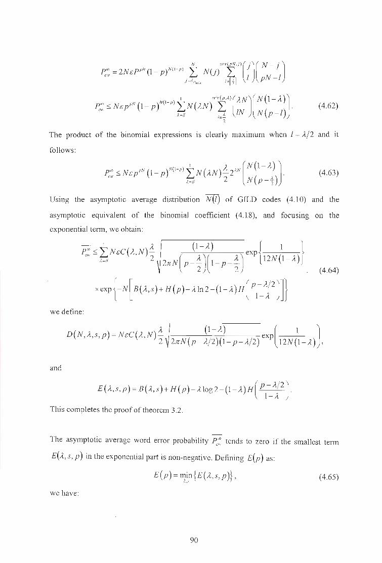
(4.62)

The product of the binomial expressions is clearly maximum when 1= AI2 and it

follows:

poo ~ Ne pN (1- )N(I-P)~ N(AN) A2AN (N (I- A) J. (4.63)ell' P P L... 2 N( A)

A=(j P-2"

Using the asymptotic average distribution N(t) of GILD codes (4.10) and the

asymptotic equivalent of the binomial coefficient (4.18), and focusing on the

exponential term, we obtain:

- I A (I-A) {I}poo <" NcC(A N)- expelV-t-t '2 (A)( A) l2N(1-A)2rcN p-- 1- p--

2 2 . (4.64)

xexp { -N[E(A,s)+ H(p)- Aln2-(I- A)H( Pj-_A2)]}we define:

D(N,A,S,p)=NcC(A,N)A (I-A) exp [ 1 J2 2rcN(p-AI2)(1- p-AI2) l2N(1-A) '

and

E(A,S,p) = B(A,S)+ H(p )-A log2 -(I-A )H(P -AI2).I-A

This completes the proof of theorem 3.2.

The asymptotic average word error probability Pe:' tends to zero if the smallest term

E(A, s, p) in the exponential part is non-negative. Defining E(p) as:

we have:

E (p ) =min {E (A, s, p )} ,A,.I

90

(4.65)

(4.66)

We can now find the BSC crossover probability threshold p which is the highest value

for which E(p) is non-negative, with the following algorithm.

1. Start with a small value ofp.

2. Calculate the minimum value E(p) of E(A,S,p) using to (4.34) and (4.12) by

varying A (and s as they are related).

3. If E(p) > 0, increase the value of p and return to 2, else Pthres = P is an

asymptotical upper bound on the crossover probability of the BSC that leads to a

vanishing word error probability ofML decoding of the GILD code.

Table 4.2 shows the value of p compared withP(C), the probability threshold for a

code achieving the capacity at the same rate for different kinds of GILD codes. GILD

codes thus achieve near-capacity performance on BSC channels when their length is

arbitrarily large.

4.4 Upper Bound on Minimum Distance for a Fixed Length

In this section, expression (4.9) of the average weight distribution of the GILD codes is

used to compute an upper bound on the minimum Hamming distance of the ensemble of

GILD codes with fixed length. The major difference with Section 4.3.2 is that

inequalities (4.13) and (4.14) are not used.

The probability that the minimum distance d H . of a linear block code C of length N111111

is lower than, or equal to, D is the probability that there exists a sequence ~ of length

N and weight I lower than, or equal to, D that is a codeword of C :

Prob (dHmill ::; D) = Prob(::I~ E GF(2)'" / w(~) = I::; D and ~ E C). (4.67)

This probability is clearly less than the sum of the probabilities that the individual

sequences ~ of the considered weight are codewords:

91

Table 4.2: BSC crossover probability threshold p of some GILD codes compared with

the threshold P(C) of the code of the same rate achieving capacity.

Constituent Code Co Value of8 Rate of the GILD Code P p(c)

Hamming 1 0.143 0.278 0.281

(7,4,3) 0.95 0.164 0.260 0.266

0.9 0.186 0.242 0.252

BCH (t=2) 1 0.355 0.164 0.165

(31,21,5) 0.95 0.371 0.156 0.158

0.9 0.387 0.149 0.151

0.85 0.403 0.142 0.145

1 0.313 0.183 0.183

0.95 0.330 0.175 0.175

Extended BCH 0.9 0.347 0.167 0.168

(32,21,6) 0.85 0.364 0.159 0.160

0.825 0.373 0.155 0.157

BCR (t=2) 1 0.619 0.071 0.074

(63,51,5) 0.95 0.629 0.068 0.071

0.925 0.633 0.066 0.070

Extended BCR I 0.594 0.079 0.081

(64,51,6) 0.95 0.604 0.075 0.078

0.925 0.609 0.074 0.077

ProbedHm•• ~ D) ~ ,ft;;, Prob(~ E C) =t(nP(i), (4.68)

where P(l) is defined as the probability that a sequence of weight I is a codeword.

We calculate P(l) for the average ensemble of GILD codes of fixed length N using

(4.8). Applying (4.9) in (4.68) leads to:

f) __

Prob(dHmin s:; D) s:; L N(l).1=1

92

(4.69)

An upper bound for the minimum Hamming distance of C is computed by taking the

right hand side of (4.69) greater than, or equal to, 1. We have:

dHmin

:s:;; ~,

where L1 is the smallest integer such that

It.N(t)J;'l

(4.70)

(4.71 )

Figure 4.6 shows this bound!':. calculated for the GILD code based on the (31, 21, 5)

BCH component code for two values of 8. The granularity of the curves is due to the

fact that all the codes considered do not correspond to the exact values of 8, as the

length of a GILD code has to be a multiple of the constituent code length. The average

minimum distance of these codes is clearly a linear function of their length. It is,

however, observed that GILD codes have lower minimum Hamming distance when

compared with the corresponding GLD codes.

4.5 GILD Codes Based on Different Constituent Codes

The definition and construction in Section 4.2 assume the sane constituent code is used.

However, GILD can also be constructed using different constituent code in the irregular

ensemble.

4.5.1 Definition

A binary GILD code with two levels based on different constituent codes is defined by

four parameters:

••

•

•

The length of the code N.

The length nl of the constituent code Cl' with dimension kl

and rate 1) .

The length n2 of the constituent code C2 , with dimension k2

and rate r2

•

The fraction, fJ (fJ < 1), of the code symbols connected to the second super-code.

93

400 -.---.--------.--.-- ------- --.--..--.-.-- _ - _-- _ ,

350

200

150

300 ..

LlC:::J

a5 250(])uc~IJl(5

E:::J

Ec

::2:

100

50

i --+-GLD

---...- GILD, theta = 0.95

-&- GILD, theta = 0.9

oo 500 1000 1500 2000 2500 3000

Length of the Code

Figure 4.6: Upper bounds using (4.71) for GILD codes based on the (31, 21,5) BCH

component code.

Assuming that Cl is used in the first super-code and C2 is used in the second super-

code, then N must be a multiple of n\ and eN a multiple of n2

.

4.5.2 Contruction

The construction of the code is also achieved through a superposition method. To

construct the parity-check matrix H of such a code, we first construct a low-density

(LD) matrix with N (~+ I~) rows and N columns, having exactly:

• eN columns with 2 ones

• N (1- e) columns with lone

94

•

•

•

N 0 h 0 h- rows WIt nl

ones III eacnl

eN oh . h- rows WIt n2 ones III eacn2

Zeros elsewhere

Then we do the following:

1. In each the N rows with nl ones, we replace the N - nl zero elements by a zeron

J

column-vector of length (nJ

- kJ), and the nonzero elements by one of the n

J

different columns of the constituent code CJ's parity-check matrix, each used

once.

2. In each of the eN rows with n2 ones, we replace the N - n2 zero elements by an2

zero column-vector of length (n2 - k2 ), and the nonzero elements by one of the

n2 different columns of the constituent code C2 's parity-check matrix, each

used once.

The LD matrix should also be constructed such that its Tanner graph contains no cycle

of length 4. If the parity-check matrix H has full rank, the total rate of the GILD code

IS:

R" = fj +er2 - e

If e=1, we obtain a GLD code based on different constituent codes.

4.5.3 Ensemble Performance

(4.72)

Let C be a binary GILD code with two levels based on different constituent codes as

defined above. Following the same reasoning as in Section Ill, it can be shown that the

average number of codewords in C having weight I is given by:

(4.73)

95

(4.74)

For I> 0, N (I) is upper bounded by:

N(I) ~ C (A, N) x e-NB'{,l.s) ,

where C (A, N) is defined by (4.11) and

B' (A,S) = H (A) + 2AS -J..-(Ilt (s) + kllog 2) -~(1l2 (s)+ k210g 2) - (1- e)log(1+ es).

nl n2

(4.75)

In (4.75), III (s)=log(gl (s)) and 1l2(s)=log(g2(s)), where gl(s) and g2(S) are the

moment generating functions of the constituent codes Cl and C2 respectively.

Asymptotically, when the length N tends to infinity, N(I) tends to zero if B'(A, s) is

strictly positive. As in Section ll, the largest value 0 of A satisfying B' (0, s) = 0 and

B' (A, s) < 0 for A > 0 gives an asymptotical lower bound on the normalized minimum

distance of the GILD code. The optimal value of s is related to the weight by:

, Il; (s) eJ1; (s ) (1 - e) eS

A =--+ + x--opl 2 2 2 1 s'n l n2 +e

(4.76)

where J1; (s) and I-t; (s) are the derivative of J11 (s) and 112 (s) relative to s. Table III

shows the values of 0 found for a GILD code based on the Hamming (31, 26, 3)

constituent code and the BCH (31, 21, 5) constituent code. As in Table 4.3, the Gilbert

Varshamov bound is also shown. It can be seen that the order in which the constituent

codes are used affects both the rate and the value of0 . As will be shown by the

simulation results in Section VI, this order also affects the code performance.

96


of some GILD Codes based on two different constituent codes compared with the

Gilbert-Varshamov bound 5 . * indicates that 5 does not exist.o

Constituent Value Rate of the 5 50Codes of8 GILD Code

Cl: Hamming 1 0.516 0.013 0.105

(31,26,3) 0.985 0.521 0.01 0.103

C2 : BCH (t=2) 0.975 0.524 0.007 0.1020.967 0.526 0.004 0.101

(31,21,5)0.965 0.527 * 0.101

Cl : BCH (t=2) 1 0.516 0.013 0.105

(31,21,5) 0.985 0.518 0.011 0.104

C2 : Hamming 0.975 0.52 0.008 0.1030.967 0.521 0.005 0.103

(31,26,3)0.965 0.522 * 0.102

4.6 ML Decoding Error Probability over the AWGN Channel

In this section, the exact average weight distribution N(z) is used to compute the

average bit error probability of maximum likelihood (ML) decoding of GILD codes.

Indeed, the interleaver acts on all the coded bits8 so that they are equally protected.

Hence from any bound on the word error probability over the AWGN channel, we can

derive an upper bound on the average bit error probability ~b without having to

compute the input-output weight enumerator function (IOWEF) as in the conventional

methods to bound the ML decoding performance of turbo-codes.

4.6.1 Union Bound

The Union-Bound (UB) for a transmission over an AWGN channel is given by:

- N I - 1 [F!i:]~b ::;I-xN(l)x-erfc Rl-h ,

H N 2 N- 0

(4.77)

R This is a major difference with classical compound codes such as parallel or serial concatenated codes or

product codes.

97

where E IN is the signal-to-noise ratio per information bit and R the GILD code rate.I> a

The classical drawback of the DB is that it is not tight and even diverges for low values

of the signal-to-noise ratio per information bit.

4.6.2 Improved Bound Based on Gallager's Bound

In [73], Duman & Saheli derived an upper bound on the word (and bit) error probability

of turbo codes with ML decoding using a modified version of Gallager's bound [72]

rather than the standard union bound. Their method is directly applicable to any linear

code, and thus to GILD codes.

The broad outlines of this bound are the partition of the code to constant-weight sub

codes, the application of Gallager's bound on each sub-code and finally the union

bound to get an upper bound on the word (and bit) error probability of the overall code.

The code C is partitioned in the set of sub-codes Cl, 1= 1, .. " N defined as the collection

of the all-zero codeword together with all the codewords of weight I. Note that Cl is not

necessarily linear. Let us denote by D i the Voronoi region associated with

fi,i = 1, .. ·,N when it is considered as a codeword of C, and denote by D; its Voronoi

region when it is considered as a codeword of Cl. It is clear that for all i:

Assuming the all-zero codeword fa is emitted, the union bound gives:

N N N

~w = I f p(y/~())dy~I I f p(y/~())dy ~ I~~:),1=1 YE/), 1=1 'iEC, YE/); 1=1

C,':;f::C"

(4.78)

(4.79)

where p(yI~()) is the likelihood of the codeword fa . Duman & Saheli applied

Gallager's bound to Pe~:,)' and found after some manipulations:

98

NREh

expNo

(4.80)

(4.81)

for the AWGN channel case, where ,B=(1-I/N)/[(1/a)-(l/NX1-p)], 0<ps1, and

0< a s 1/(1- p). a and ,B are two parameters that have to be optimized to find the

lowest value ofPe~:? .

Consequently, using the average weight distribution N(z) of the GILD codes, we have

the following improved upper bound on the ML decoding bit error probabilities:

- ~ I . (/)~h S LJ- lllin ~w,_ N O<pSI

1-1 O<asJ/(I-p)

where Pe~~) is equal to the expression (4.80) where N(z) is replaced by N(z).

4.6.3 Tangential Sphere Bound

An improved version of the tangential bound of Berlekamp [74] has been presented by

Poltyrev ([75] and [76]) and applied to turbo-codes by Sason and Shamai ([77] and

[78]). This tangential sphere bound is tighter than the Duman & Saheli bound, and its

properties follow the central inequality,

Prob( A) s Prob(~ E B, A) + Prob(~ \l B). (4.82)

In the case of the tangential sphere bound, A is an event that represents a message

decoding error, B is an N-dimensional cone with a half angle e and

radius r = JNEs tan e, and ~ is the noise vector added to the transmitted signal. The

tangential sphere bound on the block error probability Pe is based only on the distance

spectrum {N(z)} of the binary linear block code C and it reads:

99

The following parameters are used in (4.83):

cr2 = No with N standing for the one-sided spectral density of the AWGN2 ' 0

, (4.84)

6, is defined to be the Euclidean distance between two signals whose corresponding

. codewords differ in 1 symbols (I::::; N) . Thus for the case of antipodal

signals 6, = 2)LEs Also, y(a,x) designates the normalized incomplete gamma

function defined as:

r (a, x) = 1 ~a) Jot ta-'e-rdt , for positive values of a, and x. (4.85)

A geometric interpretation of the tangential sphere bound is presented in Figure 3.7. The

upper bound (4.83) is valid for all positive values of r and thus the optimal radius ro

(or equivalently Bo )' in the sense of achieving the tightest upper bound, is determined

by nullifying the derivative of the right hand side of the bound (4.83), yielding the

following optimisation equation:

100

(4.86)

f) -I, =COS

6, 12rni21--'-4NEs

The bit error probability bound on the ensemble of GILD code IS obtained by

replacing N(I) by 1/N(z)x N(z) in (4.83) and (4.86).

r

Figure 4.7: Illustration of the tangential sphere bound.

4.7 Decoding of GILD Codes

GILD codes are not LDPC codes, and thus cannot be decoded with the belief

propagation or sum-product algorithm (SPA). The decoding of GILD codes is based on

iterative soft-input soft-output (SISO) decoding of individual constituent codes. For low

rate GILD codes, exploiting the fact that the constituent code usually has a small code

length and high code rate, a trellis-based algorithm can be used to obtain high error-

101

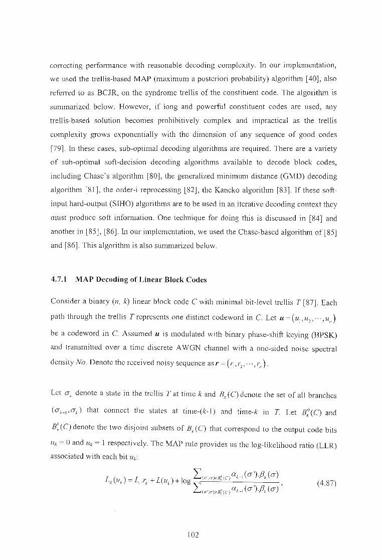
correcting performance with reasonable decoding complexity. In our implementation,

we used the trellis-based MAP (maximum a posteriori probability) algorithm [40], also

referred to as BCJR, on the syndrome trellis of the constituent code. The algorithm is

summarized below. However, if long and powerful constituent codes are used, any

trellis-based solution becomes prohibitively complex and impractical as the trellis

complexity grows exponentially with the dimension of any sequence of good codes

[79]. In these cases, sub-optimal decoding algorithms are required. There are a variety

of sub-optimal soft-decision decoding algorithms available to decode block codes,

including Chase's algorithm [80], the generalized minimum distance (GMD) decoding

algorithm [81], the order-i reprocessing [82], the Kaneko algorithm [83]. If these soft

input hard-output (SIHO) algorithms are to be used in an iterative decoding context they

must produce soft information. One technique for doing this is discussed in [84] and

another in [85], [86]. In our implementation, we used the Chase-based algorithm of [85]

and [86]. This algorithm is also summarized below.

4.7.1 MAP Decoding of Linear Block Codes

Consider a binary (n, k) linear block code C with minimal bit-level trellis T [87]. Each

path through the trellis T represents one distinct codeword in C. Let u= (u U . .. U )l' 2' '11

be a codeword in C. Assumed u is modulated with binary phase-shift keying (BPSK)

and transmitted over a time discrete AWGN channel with a one-sided noise spectral

density No. Denote the received noisy sequence as r = (1' l' ... l' )I' 2' '11·

Let (Jk denote a state in the trellis Tat time-k and Bk (C) denote the set of all branches

((Jk_1' (Jk) that connect the states at time-(k-l) and time-k in T. Let B~ (C) and

B~ (C) denote the two disjoint subsets of Bk (C) that correspond to the output code bits

Uk = 0 and Uk = 1 respectively. The MAP rule provides us the log-likelihood ratio (LLR)

associated with each bit Uk:

(4.87)

102

4Ewhere the channel reliability factor Le = --' (Es denotes the energy per symbol), L(u,J

No

P(uk =1) h' d . (487) tis the a priori value of log about Uk. The t Ir term III . represen sP(uk = 0)

extrinsic information,LexfI'(uk), in which forward recursion metric ak(a) and backward

recursion metric f3k (a) are recursively calculated as:

ak(a) = I ak_l(a').exp«Lc·rk+L(uk))·xk/2) ,(a',a)EBk (C)

and

f3k-1 (a') = I f3k (a).exp«Le·rk + L(uk)).xk/2),(a',a)EBd C )

(4.88)

(4.89)

respectively, where Xk = 2lk - 1 and lk E {O, I} represents the label of the branch

(a',a). In the iterative decoding, only the extrinsic information can be passed on to a

subsequent decoder as a priori value L(u,J.

4.7.2 Chase-Based Decoding Algorithm

The second algorithm described in [80] is used to produce a set of codewords which are

used to calculate the extrinsic information required in iterative decoding. The Chase

decoder generates 2l"Iy,'J test patterns, where d H is the minimum Hamming distance of

the component code. The test patterns form the set of sequences of length n, the length

of the component code, containing all binary combinations in the ld1j{J least reliable

positions in the soft-input to the decoder. The p ~ ld1j{Jleast reliable positions can be

considered as in [85], leading to 2" test patterns. Test sequences are created by adding

the test pattern to the hard threshold decisions on the soft-input (using modulo 2

addition). Each test sequence is then algebraically decoded to produce a list of possible

codewords. If an extended block code is used then the codeword consists of an inner

block code with an overall parity added. Only the inner code is used in the search for the

p least reliable positions. The Chase decoder algebraically decodes the test sequences

for the inner code. It then calculates an overall parity bit for the decoded inner codeword

to produce the extended codeword.

103

Once the set of codewords containing the closest codewords to the received vector is

produced by the Chase decoder, the closest codeword in the Euclidean distance sense to

this vector is selected as the decision. After the decision is obtained, the reliability of

each of its components is calculated to generate soft-decision at the output of the

decoder. The soft-output is required so that the extrinsic information generated can be

passed to the next decoder in an iterative decoding scheme. See [85] and [86] for more

details.

4.7.3 Iterative Decoding of GILD Codes

GILD codes can effectively be decoded using the following decoding scheme. For each

bit, we compute its probability given its received sample considering that it belongs to

the super-code Cl. We use N / n SISO decoders working in parallel on the N / n

independent constituent codes of Cl. Each decoder is implemented using one of the

above algorithms. This step generates for each coded symbol an a posteriori probability

and an extrinsic probability. The latter one is fed through the interleaver to the second

step as a priori information for the ()N / n SISO decoders working on the ()N / n

constituent codes of e2. This process is iterated on each super-code: Cl ~ e2 ~ Cl ~

e2~ Cl ~ ... until the preset maximum iteration number is reached or a stopping

criterion is satisfied.


Iterative decoding of several GILD codes suitable for small frame systems for an

AWGN channel with binary input was simulated. The construction each code is

achieved as described in Section 4.2 using a random interleaver. For each code the

constituent code are decoded using the MAP algorithm. In the decoding process, we

limited the number of iteration to 10 unless otherwise stated. The performances are

given in tenns of the bit-error rate (BER) versus the normalized signal-to-noise ratio

(SNR) per information bit. At each SNR value, at least 100 codeword are detected.

104

The first code has length N =961. Its constituent code is the (31,21,5) BCH code. Its

performance is shown in Figure 4.8 for different values of (), and compared with the

corresponding GLD code. The rate of the GLD code is 0.355 and the rates of the GILD

codes are 0.386, 0.417, 0.428, and 0.438 for () =0.903, () =0.806, () =0.774, and

() = 0.742 respectively. This corresponds to an increase in the code rate of about 9%,

17%, 21 %, and 23% respectively. It can be observed that the GILD codes with

() =0.903 and () =0.806 outperform the GLD code, with an improvement of about 0.3

dB and 0.6 dB at a BER of 10-4 respectively. It can also be observed that the

performances of the GILD code with () = 0.774 and () = 0.742 start to degrade at

medium to high signal-to-noise ratio. This is probably due to the fact that for this values

of () , the GILD code has a much smaller minimum distance.

In Figure 4.9, the performance ofa GILD code oflength N= 961 based on two different

constituent codes is shown for different values of (). The constituent codes are the

(31,21,5) BCH code and the (31,26,3) Hamming code. The BCH code is used in the

first super-code and the Hamming code is used in the second super-code. Compared to

the first case where the BCH code is used in both super-codes, this results in higher rate

codes. The rate of the GLD code is 0.516 and the rates of the GILD codes are 0.532,

0.547, and 0.558 for () =0.903, () =0.806, and () =0.742 respectively. It can be

observed that, at a BER of 10-4, the GILD code with () = 0.806 outperforms the GLD

code by about 0.25 dB. In Figure 4.10, the constituent codes are used in the reverse

order, i.e. the Hamming code is used in the first super- code and the BCH code is used

in the second super-code. For the same value of () , this results in further increase in the

code rate. However, there is a degradation in the code's performance and the allowable

values of (). This reveals the interesting finding that if two different constituent codes

are used, the stronger code should be used in the first super-code.

105

1.00E-01

1.00E-02Q)

roCl::....gw~

II)

1.00E-03

1.00E-04

1.00E-05

0.5

~GLD

- GILD, theta = 0.903

,-.- GILD, theta =0.806

---*- GILD, theta = 0.774

-lIE-GILD, theta = 0.742

1.5

SNR (dB)

2 2.5 3

Figure 4.8: Simulated performance of four GILD codes and the corresponding GLD

code built from the (31,21,5) BCH constituent code, length N = 961, AWGN channel.

106

1.00E+00

1.00E-02

(\)

&....g 1.00E-03w

1.00E-04 -

1.00E-05

1.00E-06

0.5

I--+-- GLD

.__GILD, theta = 0.903!

~ GILD, theta =0.8061

- - -+- -- GILD, theta =0.742!

1.5

SNR (dB)

2 2.5

Figure 4.9: Simulated perfonnance of three GILD codes and the corresponding GLD

code built from two different constituent codes. The (31,21,5) BCH (used in the first

super-code) and the (31,26,3) Hamming code (used in the second super-code), length

N = 961, AWGN channel.

107

1.00E+00

-+-GLD

----.- GILD, theta = 0.935

. ----*"- GILD, theta = 0.903.

1.00E-04

1.00E-01 ~=;;;;;;;;;=t-_

1.00E-02IDm

0:::'-e'-

UJ......co

1.00E-03

2.521.5

SNR (dB)

1.00E-05 '------------------------------'

0.5

Figure 4.10: Simulated performance of two GILD codes and the corresponding GLD

code built from two different constituent codes. The (31,26,3) Hamming code (used in

the first super-code) and the (31,21,5) BCH code (used in the second super-code),

length N = 961, AWGN channel.

108

In Figure 4.11, a GILD code of length N =1005, e= 0.910, and rate 0.491 built from

the (15,11,3) Hamming code is compared with two LDPC codes of length 1008 and

rate 0.5 constructed using the progressive edge growth (PEG) algorithm [50, 169]. The

PEG construction creates matrices with very large girth and, to the best of our

knowledge, yields the best binary LDPC codes at short block lengths. The regular

LDPC code has a column weight of 3. The code-node degree distributions used by the

PEG algorithm to generate the LDPC code are designed by the density evolution [19]

approach and are given in [60]. Note that, in the PEG algorithm, the check-node

distribution is not needed as the check-degree sequence is made as uniform as possible

by the algorithm. To the best of our knowledge, this irregular PEG LDPC code is the

best known code of this block length and rate to date [169, 170]. The LDPC codes are

decoded using the SPA algorithm with the maximum number of iterations in each

simulation set to 100 and the maximum number of iterations in the decoding process of

the GILD code is set to 20. It can be observed that, at a BER of 10-5, the GILD code

outperfonns the regular LDPC code by about 0.25 dB and is less than 0.1 dB from the

irregular one. The significance of this result should not be underestimated, considering

that the GILD code is constructed using a random interleaver. It can be anticipated that

if the code is carefully designed, using a deterministic interleaver that presents good

properties in terms of iterative decoding, its performance can be further improved. Thus,

variations of GILD codes may be able to match and even beat the best LDPC codes for

small block lengths.

109

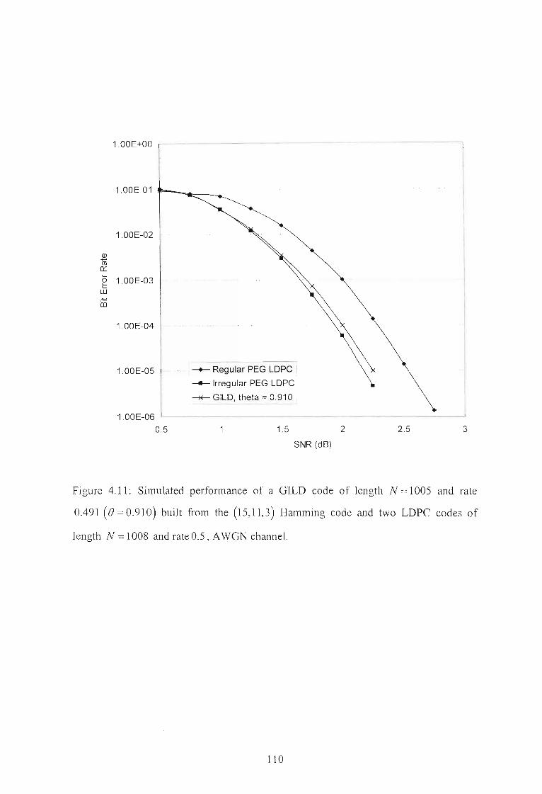
1.00E+00

1.OOE-O1 r-""*=:----...

1.00E-02

Q)

ro0::L-

1.00E-030L-

w-05

1.00E-04

1.00E-05 -'. - Regular PEG LOPC i .- Irregular PEG LDPC i

- GILD, theta =0.910

32.51.5 2

SNR (dB)

1.00E-06 '-- ---'- ~_ ____J

0.5

Figure 4.11: Simulated performance of a GILD code of length N = 1005 and rate

0.491 (B=0.910) built from the (15,11,3) Hamming code and two LDPC codes of

length N =1008 and rate 0.5, AWGN channel.

110

In Figure 4.12, the performance of the first code with 8 = 0.903 is shown for different

iteration steps, and compared to the various bounds described in Section 4.5. It can be

seen that there is a loss in a large range of Eh / No between the simulation results and

the bounds. This loss is probably due to the interleaver choice and the decoding. The

influences of the interleaver choice and the decoding algorithm on the performance of

GILD codes are subject of further research.

43.531.5 2 2.5

SNR (dB)

-----,____ Iteration # 2 I

~ Iteration # 4

--Union Bound

- - - - Tangential Sphere Bound--------

• Iteration # 1

,---...- Iteration # 3

)lE Iteration # 10

- - - - - . Duman & Saheli Bound---

1.00E+OO

1.00E-01 .""

1.00E-02 \\

\QJ

ro 1.00E-03 \n::

L... \0L...L... \ill..... 1.00E-04

\ro\

1.00E-05

1.00E-06

1.00E-07

0 0.5

Figure 4.12: Bit Error Probability upper bounds and simulations results for the GILD

code based on the (31,21,5) BCH component code. 8 = 0.903.

III

4.9 Conclusions

In this chapter, we have investigated the construction of new families of error-correcting

codes based on irregular low-density parity-check codes which we called GILD codes,

where small linear block codes are used as component codes instead of single-error

detecting parity-check codes. It is proved that there exist such GILD codes for which

the minimum Hamming distance is growing with the block length, and a lower bound of

the minimum distance is given. It is shown that GILD codes performance approaches

the channel capacity limit. The decoding of GILD codes is based on SISO decoding of

the component code and the appropriate algorithm to achieve this depends on the length

and dimension of the component code. Iterative decoding of GILD codes after

transmission over an AWGN channel indicates they perform better than the

corresponding GLD codes. GILD codes also have a higher rate than the corresponding

GLD codes. On the other hand, like GLD codes, GILD codes have fewer problems with

an error floor because of their large minimum distance. Simulation results also show

that variations of GILD codes may be able to match or beat the best LDPC codes for

small block lengths.

112

CHAPTERS

A LOW-WEIGHT TRELLIS-BASED SOFT-INPUT SOFT

OUTPUT DECODING ALGORITHM FOR LINEAR

BLOCK CODE

In this chapter, reduced-complexity trellis-based soft-input soft-output (SISO) decoding

of linear block codes is considered. A new low-weight subtrellis based SISO decoding

algorithm for linear block code to achieve near optimal error performance with a

significant reduction in decoding complexity is presented. The proposed scheme is

suitable for iterative decoding and has the following important features. An initial

candidate codeword is first generated by a simple decoding method that guarantees a

sllccessful decoding. By successful decoding, we mean that the candidate codeword is

indeed a codeword, but not necessarily the transmitted codeword. A low-weight

subtrellis diagram centered around the candidate codeword is constructed. The MAP

algorithm is then applied to the subtrellis. The generated extrinsic information is used as

apriori information to improve the generation of a candidate codeword for the next stage

of iteration. Simulation results indicate that the proposed algorithm provides a

significant improvement in error performance over Chase-based algorithm and achieves

practically optimal performance with a significant reduction in decoding complexity.

The organization of this chapter is as follows: in the next section an introduction is

presented. The trellis representation of linear block codes is briefly discussed in Section

5.2. An algorithm for purging a minimal trellis diagram of a linear block code to yield a

subtrellis diagram is presented in Section 5.3. In Section 5.4 a method to build a

subtrellis diagram using supercodes is described. The SISO algorithm is presented in

Section 5.5. Simulation results on the error performance of a GILD code are presented

in Section 5.6, and finally, conclusions are drawn in Section 5.7.

113

5.1 Introduction

The problem of finding computationally efficient and practically implementable soft

input soft-output (SISO) decoding algorithms for block codes is still an open and

challenging problem. Any SISO decoding of block codes using a full code trellis can be

primitively complex. This is especially true if these codes are used as component codes

in compound coding scheme such as GILD and GLD codes discussed in this thesis. One

alternative approach is to use a list-based decoding algorithm as discussed in the next

chapter. List-based decoding algorithms try to produce a list containing the closest

codewords to the soft input by encoding or decoding test sequences and calculate

extrinsic information using this list. However, this method cannot be extended

effectively to all classes of codes. Moreover, it is sub-optimal.

To overcome the state and branch complexity problems of large trellises for long block

codes, several new approaches have been proposed [146]-[151]. Most recently, Moorthy

et al. [95] have shown that the minimum-weight subtrellis of a code is sparsely

.connected and has much simpler state and branch complexities than the full code trellis.

Based on this fact, they proposed a minimum-weight subtrellis-based iterative decoding

algorithm for linear block codes to achieve suboptimum error performance with a

drastic reduction in decoding complexity compared with a trellis-based MLD algorithm,

using a full code trellis. This algorithm was improved by Koumoto et al.[152].

In this chapter a new low-weight subtrellis based SISO decoding algorithm for linear

block code to achieve near optimal error performance with a significant reduction in

decoding complexity is presented. By Iow-weight subtrellis, we mean a subtrellis of the

code trellis that consists of only codewords of Iow weights with respect to a given

codeword. The proposed scheme is suitable for iterative decoding and has the following

important features. An initial candidate codeword is first generated by a simple

decoding method that guarantees a successful decoding. By successful decoding, we

mean that the candidate codeword is indeed a codeword, but not necessarily the

transmitted codeword. The decoding method is basically the syndrome computation of

test pattems that are constructed based on the reliability of the soft-decision received

symbols. In contrast to the algorithm in [95], no algebraic decoding algorithm is used. A

114

low-weight subtrellis diagram centered around the candidate codeword is constructed.

The subtrellis diagram is sparsely connected and much simpler than the full trellis

diagram of the code. The MAP algorithm is then applied to the subtrellis. The generated

extrinsic information is used as apriori information to improve the generation of a

candidate codeword for the next stage of iteration. Instead of a theoretical analysis of

the proposed algorithm some simulation results that indicate that it achieves practically

optimal performance with a significant reduction in decoding complexity compared

with the MAP based on the full trellis diagram of the code are presented.

5.2 Preliminaries

In this section the trellis representation of linear block codes is briefly discussed. In

1978, Wolf [128] showed that every (n,k) linear block code has an n-section trellis

diagram. In recent years, there have been exciting developments in trellis structure of

linear block codes [129] - [139]. Some well-known codes have been proved to have

relatively simple trellis structures. A trellis is a directed graph T = (S, W), where the

set S = {o-} of nodes (states) of the graph is decomposed into a un~on of n +1disjoints

subsets S = So USI U... USII that are called levels of the trellis. Similarly, there exists a

partitioning of the sets of branches (edges) W = {wJ = ~ UW; U... U~, . A node 0- E S,

of level t may be connected with a node 0-' E S'+l of the level t +1 by one or several

branches. Each branch w, is directed from a node 0- of level t to a node 0-' of the next

level t +1. We assume that the end levels have only one node, namely So = {o-o} and

SII = {o-II }· A trellis is a compact method to represent all codewords of a code. Each

branch of the trellis wr is labeled by a code symbol v, (w/). Each distinct codeword

corresponds to a distinct path in the trellis, i.e., there is a one-to-one correspondence

between each codeword C III the code and a path JV III the trellis:

c( JV) = Cl (wl ), ... , clI(w

lI) •

For a linear code, a minimal trellis can be obtained using its parity-check matrix [128].

Such a trellis is called syndrome trellis. Let H = (hi'···' h,J denote the parity-check

115

matrix of C, where h; denotes the ith column vector. The term minimal trellis indicates

that this trellis has the minimal possible number ISI of nodes. The nodes of the trellis are

identified by (n - k) -tuples with elements from the binary field IF2 = {O, I}, with 0

referring to the all zero n - k -tuple. At level t = °and level t = n the trellis contains

one node, the all zero node CYa = CY" = O. The following algorithm describes a trellis

construction which differs from that of [128], but results in the same graph.

• Step 1: construct the head of the trellis, i.e., all states and branches of the levels

t = 0"",L"~I J. Set CYa= O. For each t =1,.··,L"~I J, the collection of nodes at

level t +1 is obtained from the collection of nodes at level t by CY'+J = CY, + c,lt,

• Step 2: Construct the tail of the trellis, i.e., all states and branches of the levels

t = n n -1 ... L.!.'..±lJ Set CY = 0 For each t = n -1 ... L.!.'..±lJ the collection of"'2· 11· "2'

nodes at level t -1 is obtained from the collection of nodes at level t by

• Step 3: Connect the head and tail of the trellis. We connect the collection of

nodes at level t = L"~J Jwith the collection of nodes at level t +1 by

5.3 Low-Weight Trellis Diagram

In the following, we considered, according to [95], purging the minimal n-section trellis

diagram T for a linear block code C to obtain a subtrellis diagram, denoted Tp

(0) ,

which consist of only the all-zero codeword and the codewords c of C such that

dll(c,O)~p, where dH (,) is the Hamming distance of two vectors. Such a trellis is

called the p -weight trellis diagram for C. We say that this p -weight trellis diagram is

centered around the all-zero codeword O.

116

For two adjacent states 0" and 0"' , with 0" E 5, and 0"' E 5'+1' let 1(0",0"') denote the set

of parallel branches connecting states 0" and 0"' . Let w, be a branch in I (0",0"') and

,,1,(w, ) denote the Hamming weight of wl

• Let a (l (0",0"')) denote the minimum

hamming weight of the parallel branches in 1(0",0"').

For any state 0" E SI with 0 ~ t ~ n, let (0") denote the mllllmum of the Hamming

weights of all paths from 0"0 to 0". We call (0") the minimum path weight to the state

0". Clearly, (0"0) =O. For every state 0" ET, (0") can be computed by an algorithm

very similar to the well-known Viterbi algorithm as follows: Assume that (0") is known

for every state in S. for 0 ~ j < t . Let 0"' be a state in SI . Then (0"') is given by:J

where

(0"') = min {(O") + a (1(0", O"'))},1'(<5')

F(O"') = {O" E SI _ I : 1(0",0"'):;t: sb}.

(5.1 )

(5.2)

The process begins with 0"0' Once (0") is determined for every state 0" E Sf' the states

in the (t + 1) th-Ievel state space 5(1+1) can be processed. This computation is repeated

unti1 (0"11) = 0 is determined.

For any state 0" E 5/ with 0 ~ t ~ n, let [0"] denote the mllllmum of the Hamming

weights of all paths from 0" to the final state 0"11' We call [0"] the minimum path weight

from 0". For every state 0" in T , [0"] can be computed recursively from O"n as follows:

assume that [0"] is known for every state 0" E Si for t < j :s; n. Let 0"' be a state in Sf'

Then [0"'] is given by:

with

[0"'] = min {[O"] + a (l(0",0"1))} ,( ;(<5')

G(0"') = {O" E 5(1+1) : I (0"',0") :;t: sb} .

(5.3)

(5.4)

Note that among all the paths passing through a given state 0" , there is a least one path

with Hamming weight (0")+[0"] and no path passing through that state has Hamming

117

weight less than (er) + [er] . Let the all-zero path be denoted by the state sequence

rT" = ero ero ... ero = er . It is clear that (ero) = [ero] =0 for O.s t .s n and for any stateVo 0' I' '11 " I f

er not in this sequence, (er) + [er] > 0 .

A systematic method of deleting states and branches in T to obtain a subtrellis which

contains all the codewords with weight up to and including p where p is a nonzero

weight in the weight profile OJ of code C is now described. This method consists of the

following rules [95].

• Rule 1: If for any state er ET, (er) + [er] > p, delete that state and all the

branches to and from er .

• Rule 2: Let er, er' be any two connected states at depths t and (t +1), O.s t .s n,

respectively. Let w, be a single branch from er to er'. If (er) + [er'] + A.(w,) > p

then, delete the branch w,.

• Rule 3: If as a result of application of Rules 1 and 2 to all the states and branches

of T any state in T has no incoming branches, then that state and all the

outgoing branches from that state are deleted. The above purging rules are

applied repeatedly until further application leaves the trellis unaltered. Let

Tp (0) denote the resultant purged trellis.

The subtrellis Tp (0) contains the following codewords of C: 1) All codewords of

weights up to and including p and 2) possibly some codewords of weight greater than

p which correspond to nonzero paths in T that diverges from and remerges with the

all-zero path more than once. For each of these paths, the weight of the partial path

between the adjacent diverging and merging states, called the side-loop, is p or less but

not zero.

Now the subtrellis diagram Tp (0) is modified so that the resultant trellis contains only

the all-zero path and all the paths which correspond to codewords of weight up to and

118

including p of C (no other paths). This resultant trellis, denoted Tp (0), is called the

p -weight trellis diagram for C. The modification of Tp (0) is done as follows:

• Step 1: Create n -1 new states q,°2"",°"_1 one at each level except the oth

and nth levels.

• Step 2: For 1::::; t < n -1, connect the state 0, to state 0'+1 by a single branch with

the 0 label. Also, connect the state 0"_1 to the final state (J" by a single zero

branch.

• Step 3: For every branch with label w:;t 0 in Tp (0) that merges into one of the

states, (J,o on the zero path (JIO, (J~," " (J~_I from any state (J , delete that branch

and create a new branch w' with the same label from (J to the state 0, .

Steps 1)-3) ensure that there is no path in the new trellis Tp(O) that after merging with

the all-zero path diverges from it again before terminating at the final state (J" .

Consequently, Tp (0) contains only the all-zero codeword and the codewords of weight

. up to and including p of C. Therefore Tp(O) is the desired p -weight trellis diagram

for C. Let Tp (0) = (S, W), where S is the set of active nodes and W is the set of

active branches. By active nodes and active branches, we mean the nodes and branches

which have not been deleted.

The p -weight trellis diagram for a linear block code C is sparsely connected and has

much smaller state and branch complexities than those of the full trellis diagram for C.

Table 5.1 shows the state complexity profile for the full trellis and two subtrellises of

the (31, 21, 5) BCH code. For this code, the minimum-weight trellis diagram (p = 5)

has a total of 1860 branches, and the 7-weight trellis diagram (p = 7) has a total of

6640 branches, whereas the full trellis has a total of 26620 branches. This reduction in

number of states and branches contributes to a significant reduction in computational

complexity.

119

Table 5.1: State complexity profile for the full trellis and two subtrellises of the (31, 21,

5) BCH code.

Trellis level Full trellis Subtrellis (p = 5) Subtrellis (p = 7)

0 1 1 1

1 2 2 2

2 4 4 4

3 8 7 8

4 16 12 16

5 32 20 28

6 64 29 47

7 128 42 75

8 256 56 116

9 512 71 170

10 1024 86 238

11 1024 102 302

12 1024 115 362

13 1024 129 408

14 1024 136 408

15 1024 139 434

16 1024 139 434

17 1024 136 427

18 1024 129 408

19 1024 115 362

20 1024 102 302

21 1024 86 238

22 512 71 170

23 256 56 116

24 128 42 75

25 64 29 47

26 32 20 28

27 16 12 1628 8 7 829 4 4 430 2 2 231 1 1 1

120

5.4 Low-Weight Trellis Diagram Using Supercodes

A low complexity approach to construct a low-weight trellis diagram is to use

supercodes. A supercode [140] of a linear code C is a linear code er such that C c er .

For the sake of simplicity, we consider only the case where we have two supercodes.

Let H ~ (~J be the parity-check matrix of the code C, where the submatrix

HI consists of the upper In;k 1row vectors of H , and H 2 consists of the lower

Ln;k Jrow vectors. Then the sub-matrices HI and H 2 define the supercodes Cl and C2 ,

respectively. Let ~(I)(O) and ~(2)(0) denote the p -weight trellies diagram of Cl and

C2

' respectively. That is, ~(I) (0) = (S(I), W(I») and ~(2) (0) = (S(2), W(2») . The

following algorithm constructs a trellis Tp (0) representing the set ~ (I) (0) n~(2) (0) . A

node in this trellis is represented by an n - k tuple (JI = ((J1(1)(J1(2») , where (JI(I) is an

I ";k 1tuple and (J?) is an L";k Jtuple.

• Step 1: set So = {O} and set t =1.

• Step 2: the set SI is constructed from the set Sf-1' the parity-check matrices HI

and H 2 , and sets ~(I) and ~(2). The collection of nodes at level t is obtained

from the collection of nodes at level t -1 by:

(J(I) = (J(I) +chI I-I I "1,1

(J(2) = (J(2) + chI I-I I 2,1

for all (JI_I E SI_I and c E IF such that (J(I) E S(I) and (J(2) E S-(2)1 2 f 1 f I'

•

•

Step 3: If t < n, then continue with the next level, i.e., increment t by one and go

to step 2.

Step 4: Remove all nodes (except (J,,) which have no outgoing branch, and

remove the corresponding incoming branches.

121

5.5 A Low-Weight Soft-Input Soft-Output Decoding Algorithm

In this section, a low-weight soft-input soft-output decoding algorithm suitable for

iterative decoding of linear block codes when they are used as component codes in a

compound or concatenated coding scheme is described. Candidate codewords are

generated one at a time based on syndrome computation of test sequences which are

constructed in a manner similar to list-based decoding algorithm. To be more specific,

error patterns are generated in a serial fashion in increasing order of bit reliability

values. Thus the ith (i =0,1,2, ... ,2" -1 , where n is the length of the codewords) error

pattern corresponds to number i in the binary number system. The bit positions are

arranged in the order of their reliabilities such that the least reliable bit is the least

significant bit and so on. After generating an error pattern, the error pattern is added to

the hard decision corresponding to the received vector, and syndrome computation is

performed on the resultant test sequence. It is important to note that, contrary to list

based decoding algorithms, no algebraic decoding algorithm is used. If the syndrome of

the test sequence is zero, then it is considered as the candidate codeword. Otherwise, the

next test sequence is generated and tested using syndrome computation.

When a candidate codeword c is generated, a subtrellis diagram T (c) that containsp

only the codewords of weight up to and including p centered around c is constructed.

First Tp (0) centered around the all-zero codeword 0 is constructed before the decoder

implementation (or design). A method of constructing Tp

(0) was presented in the

previous section. Tp (c) is isomorphic to Tp (0) and is obtained by adding the candidate

codeword c to every codeword in Tp(O). The MAP (maximum a posteriori probability)

algorithm [40], also referred to as BCJR, is then applied to the subtrelis diagram Tp

(c) .

The algorithm was summarized in Chapter 4. Other trellis-based SISO decoding

algorithms, optimal or suboptimal, such as Log-MAP, Max-Iog-MAP [141] or even

SOYA [142], can also be used. The generated extrinsic information is used a priori

information to improve the generation of a candidate codeword for the next stage of

iteration.

122


The proposed low-weight subtrellis based SISO decoding algorithm has been applied to

GILD codes discussed in the previous chapter. The GILD code of length N = 961, () =

0.806 based on the (31, 21, 5) BCH code was used. We assumed AWGN channel BPSK

signaling. The BER performance of this code using the proposed algorithm is shown in

Figure 5.1 for p = 6, and p = 7. It is observed that the performance improves with p,

with diminishing return. No significant improvement in performance was observed for

greater values of p. The performance of the proposed algorithm is now compared with

the MAP algorithm applied to the full code trellis. For the proposed algorithm p = 7.

The performance of both algorithms is shown in Figure 5.2. We see that the error

performance of this code based on the proposed algorithm falls on top of its

performance using the MAP algorithm applied to the full code trellis. Thus the proposed

algorithm achieves practically optimal error performance with a significant reduction in

computational complexity. In Figure 5.3 the BER performance of the proposed

algorithm is compared to that of the Chased-based algorithm presented in the previous

chapter, with each Chase decoder using a set of 16 test sequences. The results show that

the proposed algorithm performs better than the Chase-based algorithm. At a BER of

10-5, the improvement in performance is about 0.13 dB.

123

1.00E+00 r·· ..···········..··..·· ..·· ·..·..·..··········..·•········ ····..·····..·····..········ ..··1

1.00E·01

1.00E-02

a:wco

1.00E-03

1.00E·04-+-Rho = 6

---e-- Rho = 5

252

Eb/No (dB)

1.5

1.00E-05 '---------------------------'

1

Figure 5.1: Simulated performance of the GILD code of length N = 961, e = 0.806,

built from the (31,21,5) BCH component code, AWGN channel, 8 iterations.

124

0:::wco

1.00E+OO

1.00E-01

1.00E-02

1.00E-03

1.00E-04 _.

1.00E-05

1 1.5

..... ~ .-

2

Eb/No (dB)

2.5

Figure 5.2: Performance of the simulated GILD using the proposed algorithm with p =

7 (solid) and the MAP algorithm applied to the full trellis (dashed) after 8 iterations in

both cases. N = 961, 8 = 0.806, built from the (31, 21, 5) BCH component code,

AWGN channel.

125

1.00E+OO

1.00E-01

'G),

1.00E-02

0:::Wa::J

1.00E-03

o.

1.00E-04

1.00E-05

1.5 2

Eb/No (dB)

2.5

Figure 5.3: Performance of the simulated GILD code using the proposed algorithm

(dashed) and the chase-based algorithm (solid) after 8 iterations in both cases. N = 961,

e = 0.806, built from the (31, 21, 5) BCH component code, AWGN channel.

5.7 Conclusion

In this chapter, a soft-input soft-output decoding algorithm for binary linear block codes

based on low-weight trellis to achieve practically optimum error performance with a

significant reduction in decoding complexity has been presented. The algorithm is

suitable for iterative decoding and can be applied to any compound/concatenated code

based on linear block codes.

126

CHAPTER 6

HIGH-PERFORMANCE LOW-COMPLEXITY DECODING

OF GENERALIZED LOW-DENSITY PARITY-CHECK

CODES

In this chapter, an efficient list-based soft-input soft-output (SISO) decoding algorithm

for compound codes based on linear block codes is presented. Attention is focused on

GLD codes. The proposed algorithm modifies and utilizes the improved Kaneko's

decoding algorithm for soft-input hard-output decoding. These hard outputs are

converted to soft-decisions using reliability calculations. Compared to the trellis-based

Maximum a Posteriori Probability (MAP) algorithm, the proposed algorithm suffers no

degradation in performance at low bit-error rate (BER), but presents the major

advantages of being applicable in cases where the trellis-based MAP algorithm would

be prohibitively complex and impractical. Compared to the Chase-based algorithm of

[85], [86], [88], [89] the proposed algorithm is more efficient, has lesser computational

complexity for the same performance and provides an effective tradeoff between

performance and computational complexity to facilitate its usage in practical

applications.

This chapter is organized as follows: First, a brief introduction to motivate the problem

is presented. Then a short review of GLD codes structure is given. The decoding

algorithm is presented in Section 6.3. In Section 6.4 the stopping criteria proposed for

preventing unnecessary computations and decoding delay are described. The simulation

model and results are presented in Section 6.5 and, finally, conclusions are drawn in

Section 6.6.

127

6.1 Introduction

GLD codes can effectively be decoded based on iterative SISO decoding of individual

constituent codes, where the code performance and decoding complexity are heavily

dependent on the employed SISO decoding algorithm. For low rate GLD codes,

exploiting the fact that the constituent code usually has a small code length and high

code rate, a trellis-based algorithm can be used to obtain high error-correcting

performance with reasonable decoding complexity. In [55], the Johansson-Zigangirov A

Posteriori Probability (APP) algorithm [90], which operates with one forward recursion

through a syndrome trellis was used, whereas the MAP algorithm [40], also referred to

as BCJR, was used in [56] and [66]. However, if long and powerful constituent codes

are used, these trellis-based solutions become prohibitively complex and impractical as

the trellis complexity grows exponentially with the dimension of any sequence of good

codes [79]. In these cases sub-optimal decoding algorithms are required. There are a

variety of sub-optimal soft-decision decoding algorithms available to decode block

codes, including Chase's algorithm [80], the generalized minimum distance (GMD)

decoding algorithm [81], the order-i reprocessing [82], the Kaneko algorithm [83], and

the improved Kaneko algorithm [91]. If these soft-input hard-output (SIHO) algorithms

are to be used in an iterative decoding context they must produce soft information. One

technique for doing this is discussed in [84] and another in [85], [88], [89]. In particular,

the Chase algorithm and the Kaneko algorithm have been considered for the decoding

of block turbo codes (BTCs) in [85] and [92] respectively.

In this chapter, an efficient SISO iterative decoding algorithm for GLD codes is

proposed. The algorithm modifies and utilizes the improved Kaneko's decoding

algorithm for SIHO decoding. Similar to the decoding strategy presented in [85], [88],

[89], [92], a list of codewords containing the closest codewords to the soft input is

generated by decoding test sequences using a simple algebraic decoder. The codeword

that is most likely is selected from the list, followed by reliability calculations to obtain

soft-decisions based on the remaining codewords in the list. To avoid algebraic

decoding resulting in a codeword already found, a simple test is proposed before

decoding of each test sequence. Each time when a new test sequence is generated, it is

tested. If the test holds, then this test sequence CaImot produce a candidate codeword

128

different from the candidate codewords already generated and hence it is useless. In this

case, the test sequence is ruled out for decoding and the next test sequence is generated

unless the test error patterns have been exhausted. This preprocessing test is very

effective since its complexity is considerably smaller than that of an algebraic decoding

operation. This procedure avoid useless decoding iterations and hence reduces the

complexity of the algorithm when compare to those used in [85], [88], [89], [92]. To

improve the average decoding speed of the GLD decoder, two simple criteria for

stopping the iterative process for each frame immediately after the bits can be reliably

decoded with no further iterations are proposed. For each decoded frame, the number of

iterations performed is determined by the number of passes before a certain condition or

rule for stopping is satisfied. The stopping conditions are hard-decision rules and are

computed based on the data available to the decoder at each iteration during the

decoding of each specific frame. Thus they require no extra data storage. More

explicitly, at the end of each iteration, the decoder performs a check on the condition for

stopping. If the condition is true, the iterative process on the frame is terminated, and

the decoded sequence from the current iteration is sent to the output; otherwise, the

iterative process continues to the next iteration. To prevent an endless loop should the

stopping rule never be satisfied, it is required that the decoder cease after the maximum

number of iterations, M.

6.2 Structure of GLD Codes

In the following the construction of GLD codes according to [56] is briefly described.

As a generalization of LDPC codes, GLD codes are also defined by a sparse parity

check matrix H, constructed by replacing each row in LDPC parity check matrix with

(11 - k) rows including one copy of the parity check matrix Ho of the constituent code

Co(n,k) , of a k-dimensional linear code of length n. The structure of the GLD parity

check matrix H is depicted in Figure 6.1. We divide H into J submatrices, HI, ... , H J ,

each containing a single column of constituent parity check matrix Ho in each column.

HI is a block diagonal matrix and produces the direct sum of N / n constituent codes,

where N is the GLD code length. All other submatrices are constructed as:

129

Hj = Tr /-1 (H I) forj = 2, ... , J, where Tr j _ 1 represents a random column permutation. A

(N, J, n) GLD code C can be considered as the intersection of J super-codes Cl, ... , C,

whose parity check matrices are the Jsubmatrices, HI, ... , HJ

, respectively. If Co(n,k)

has a rate r = k/n and the parity check matrix H has full rank, the total rate of the GLD

code is:

R=l-J(l-r). (6.1)

In case of smaller rank, the rate is increased accordingly. However, with increasing

block length N, (6.1) gives a good approximation of the actual rate of the code.

It has been shown that binary GLD codes with only J = 2 levels are asymptotically good

[55], [56], [66]. Furthermore, GLD codes with 2 levels have the highest code rate and

simple decoder structure. Thus in this work, only the decoding of (N, 2, n) binary GLD

codes based on primitive binary BCH codes is considered. For practical applications,

efficient GLD codes can be built from primitive shortened or extended binary BCH

codes.

")

if

N

Figure 6.1: Structure of a GLD parity-check matrix.

130

6.3 Proposed Algorithm

In the proposed algorithm, each component code is decoded using the improved Kaneko

algorithm [91], followed by reliability calculation to convert the hard-output of the

decoder to a soft-output.

The improved Kaneko algorithm (IKA), which is summarized below, is a candidate

codeword generation algorithm. The basic concept is to reduce the average complexity

by selecting input vectors for hard-decision bounded-distance decoding so that the

resultant codewords are likely to be transmitted. This concept is quite similar to that of

Chase algorithms [80] except that the complexity of Chase algorithms is fixed while its

complexity is probabilistic.

6.3.1 Soft Decision Decoding of Linear Block Codes Using the Improved Kaneko

Algorithm

Suppose a binary linear block code C of length 11, message length k, and minimum

distance d, denoted as an (n, k, d) code is used for error control over the additive white

Gaussian (AWGN) channel using binary phase-shift keying (BPSK) signalling. Let

C = (Cl' c2 , ... , c lI ) be the transmitted codeword which is the output of the encoder, where

Cj is an element of GF(2). For BPSK transmission, C is mapped into a bipolar sequence

x = (XI'X 2 , ... , xJ with x j = S(c,) E {± I} for 1::; i::; n, where S is a function defined as:

{

-IS(c j ) = '

+1,

Cj =0

c j = 1(6.2)

Suppose x is transmitted; at the receiver, the demodulator generates the reliability

sequence a = (ai' a 2 , ••• , an) from the received sequence Y = (YI' Y2 ,... ,Yn), where Yj

is the received signal when Xi is transmitted. The reliability of the component Yj is

defined using the log-likelihood ratio (LLR) of the decision Yi as:

131

The received vector y at the output of the AWGN channel is given by:

y=x+g,

(6.3)

(6.4)

where components gi of g = (gp g 2"'" gJ are AWGN samples of standard deviation

a. Let yH =(yt ,Y~ ,... , y:,-I )be the binary hard decision received sequence obtained

from y using the hard decision function given by:

H ={O,Yi 1,

i = 1,2, ... , n. (6.5)

We refer to lail as the reliability ofYiH . A larger la,l implies that the hard decision YiH

is more reliable. We use jYi I as the reliability measure of the received symbol Yi since

this value is proportional to the log-likelihood ratio associated with the symbol hard

decision. It is known that the maximal-likelihood decoder selects cm as an estimate if

S(Cm)·a~S(Cm.)·a for all m':j:.m [93], [94]. The objective becomes to find a

codeword maximizing the dot productS(c m )·a.

For some positive integer t ~ L(d -1);2J, a hard-decision bounded-distance decoder

decodes yH to a codeword C satisfying d Ii (y H ,C ) ~ t if it exist, where LxJdenotes the

largest integer not greater than x, and dIi (a, b), the Hamming distance between a and

b . If no codeword C satisfying d Ii (y H ,C ) ~ t exist, decoding failure occurs. The

positive integer t is the error-correcting capability of the code with hard-decision

bounded-distance decoding. In the following, bounded-distance decoding always means

hard-decision bounded-distance decoding and it is assumed that there exists an efficient

bounded-distance decoding for C with error correcting capability t. Furthennore, for

convenience, it is assumed that components of all vectors are numbered in the order of

increasing reliability, so that if i ~ j , la,1 ~ la} I.

132

L t { (r)} = °12 ... e(r) = (e(r) e(r) ... e(r)) be a sequence of binary vectors of lengthe e ,r "" 1 , 2' '"

. . fI (r) (r+l) fI 11 .n. Let J; and 11 be two functIons WhICh trans er e to e as 0 ows.

and

{

a, i < A,{' ( (r)) _ (,.+1) ("+1) = 1 i = 1

J 1 e - e , ej , /'1 '

e~") i > A,

(6.6)

where

{

a,f ( (,.)) = (r+l) (,.+1) = 1

2 e e, e, ,(,. )

ei

i<~

i=~ ,

i>~

(6.7)

and

') =min(ile(r)=O ande(r) =1 2~i~n-t)./L.:2 I' 1-1'

(6.8)

(6.9)

Note that J; is a simple binary counting function.

For each eH, °~ r < 2/1-1, define a vector

-(,.) _ (-(r) -(r) ... -(r))e - el , e2 , , ell

such that

(6.10)

where

{(,.)e. ,

-(,.) = I'ej ,

0,

i < J-l

f.-l~i<f.-l+t,

i?'f.-l+t

(6.11)

J-l=max(ile~r) =1, l~i~n-t)

for r ? 1 and f.-l = 0 for r = 0 .

(6.12)

Let c(r) be the output of the bounded-distance decoder when yH EB e(r) is an input

vector. If the output of the bounded-distance decoder is not a codeword (for example,

when decoding failure occurs), c(r) is not defined. Then define ,1,. by:

133

t'1r

= max S (c(i)). 0. .O~I$r

(6.13)

The improved Kaneko algorithm is described as follows, where W H (a) denotes the

Hamming weight of a and c the estimation of the transmitted codeword, respectively.

1. Initialization: set r =0, Lt_I = -CXJ .

2. Repeat the following procedure in order r = 0,1,2,···:

If Ltr

_1

< S(yU EBe(I')).o., then

Update LtI' and c=c (I') if LtI' > Ltr _1 .

Otherwise, set e(I'+I) =.f2 (e(r)).

The main difference between this algorithm and the one in [83] is the use of the

functions It and .f2 to generate input vectors for hard-decision bounded-distance

decoding. The algorithm in [83] uses only It .The function .f2 avoids trial by which the

bounded-distance decoder never outputs a codeword maximizing the likelihood

function.

Example J: Suppose code C is the (15, 7, 5) Bose-Chaudhuri-Hocquengham (BCH)

code, whose generator polynomial is g(x) = x 7 + x 4 + x 2 + X + lover GF(2). We now

decode y whose reliability vector, without reordering components, is 0.' = (-1.82, -1.26,

-0.08, -1.24, -0.70, -1.42, -0.70, -1.42, -0.54, -0.40, -0.36, -1.66, 0.24, -2.02, -0.32, 1.04,

-0.48). The reliability vector, whose components are numbered in the order of

increasing reliability, is 0. = (-0.08, 0.24, -0.32, -0.36, -0.40, -0.48, -0.54, -0.70, 1.04, -

1.24, -1.26, -1.42, -1.66, -1.82, -2.02) and the hard-decision vector of y is yU =

(010000001000000). The process of the decoding algoritlm1 with a bounded-distance

decoder with error-correcting capability t = 2 is presented in Table 6.1. In this example,

134

the bounded-distance decoding is applied seven times and the number of e' s generated

during the decoding is 12.

Table 6.1: An example of decoding procedure for (15, 7, 5) BCH code using the IKA.

r err) S(yH EEl e(r»).a ~r-Ix(r) S(x(r»).a function

0 000000000000000 12.94 -co 000000000000000 11.02 ;;

1 100000000000000 12.30 11.02 failure - ;;

2 010000000000000 11.74 11.02 000000000000000 11.02 ;;

3 110000000000000 11.58 11.02 000000000000000 11.02 ;;

4 001000000000000 11.42 11.02 failure - ;;

5 101000000000000 11.26 11.02 111100001001000 9.22 ;;

6 011000000000000 10.94 11.02 - ;;

7 000100000000000 11.10 11.02 010111001000000 11.10 ;;

8 100100000000000 10.94 11.10 - ;;

9 010100000000000 10.62 11.10 - 12

10 001100000000000 10.46 11.10 - ;;11 000010000000000 10.74 11.10 halt

6.3.2 Test Error Patterns

A key element in the above algorithm is a set of test error patterns and their efficient

utilization in the generation of candidate codewords through a simple algebraic

decoding. The choice of the test error patterns detennines the perfonnance and

effectiveness of the above algorithm. It is obvious that only the most probable error

patterns should be used as the test error patterns. Moreover, if many test error patterns

generate the same codeword, only one should be used to decrease the time complexity

of the algorithm.

135

Again, Let err) be the output of the bounded-distance decoder when yH EB err) is an

input vector. If the output of the bounded-distance decoder is not a codeword (for

example, when decoding failure occurs), err) is not defined. A test error pattern err) is

said to be decodable if err) is defined. Two distinct error patterns, err) and eCt ) , are said

to be equivalent if they are both decodable and if err) = e Ci ). Let err) be a decodable

error pattern and let Q(e(r)) denote the set of all test error patterns, which are equivalent

to e(r). Since all the test error patterns in an equivalence class generate the same

candidate codeword, only one should be used. How to partition the set of error patterns

into equivalent classes affect the efficiency of any decoding algorithm that utilizes test

pattern set such as the one described above and those in [80], [81], and [83]. Lemma 6.1

characterizes a simple test, which can be performed before the decoding of each test

sequence to determine whether the associated test error pattern is equivalent to a test

error pattern already used.

Lemma 6.1: For some r such that r > 0 and some j such that 0 :S j < r, assuming that

the error patterns err) and eCt )are both decodable, i.e. err) and eCl )are both defined, then

e(r) and eCl ) are equivalent if and only if d H(y(r) EB e(r), eCl)):s t .

Proof First, we show that if err) and eCl ) are equivalent, then

d H(y(r) EB e(r), eCl)):s t .

Since

dH (y(r) EB e(r), e(/)):s dH (y(r) EB e(r), e(r)) + dH

(e(r), eCi))

:S t + d H ( e(r), eCi ))

Suppose

:S t . (6.14)

t<dH(y(r)EBe(r), eU)), (6.15)

equations (6.14) and (6.15) would then imply that t < t . This contradiction shows that

d ( (r) r.:p (r) Ct))< h (r) d Cl) . .I-I Y Q7 e , e - t w enever e an e are eqUIvalent. ThIS proves the first part

of the Lemma.

136

Next, we show that if the condition d H(y(r) EB e(r), e(j)).:s; t holds, then e(r) and e(j) are

equivalent.

dH(y(r)EBe(r), e(I)).:s;dH(y(r) EBe(r), e(r))+dH(e(r), e(l))

.:s;t+dH(e(r), eU)). (6.16)

Suppose e(r) and e(j) are not equivalent, i.e. e(r) and e(j) are different. We show in

Appendix B that

(6.17)

(6.18)

Hence, (6.17) becomes:

dH(/r) EBe(r), eU)).:s;dH (e(r), e(I))+3t,

contradicting the fact that the bounded distance decoder can correct at most terrors.

This contradiction shows that whenever d H(y (r) EB e er) , e (j) ).:s; t holds, e(r) and e(j) are

equivalent. This proves the second part of the Lemma.

Assume that yH EB e(r) IS decoded by bounded-distance decoding m the

order r = 0, 1, 2, "', then Lemma 6.1 provides a simple preprocessing test which can be

used to avoid bounded-distance decoding resulting in a codeword already found. Prior

to the decoding of each test sequence, it is required to check the Hamming distances

between yH EB e(r) and the codewords already found. If any of these Hamming

distances is less than or equal to t, then bounded-distance decoding of yH EB e(r) is not

needed. This procedure decreases the number of times to apply bounded-distance

decoding and hence the decoding delay of the algorithm. We will see that it improves

the perfonnance of the iterative decoding algorithm as well. Note that this test for

eliminating useless test error patterns requires considerably less computational

complexity than that of the bounded distance-t decoding. A different procedure for

generating test error patterns is also presented in [95].

In Table 6.2, the process of the decoding algorithm with the above preprocessing test

applied to example 1 is presented. It can be noticed that the bounded-distance decoding

137

is applied five times instead of seven, thus reducing the time complexity of the decoding

algorithm.

Table 6.2: An example of decoding procedure for (15, 7, 5) BCH code of example 3.1

using the IKA with the preprocessing test.

r e(r) S(yH EEl e(r)).a ~r-Ix(r) S(x(r)).a function

0 000000000000000 12.94 -00 000000000000000 11.02 J;

1 100000000000000 12.30 11.02 failure - J;

2 010000000000000 11.74 11.02 - 11.02 J;

3 110000000000000 11.58 11.02 - 11.02 J;

4 001000000000000 11.42 11.02 failure - J;

5 101000000000000 11.26 11.02 111100001001000 9.22 J;

6 011000000000000 10.94 11.02 - 12

7 000100000000000 11.10 11.02 010111001000000 11.10 J;

8 100100000000000 10.94 11.10 - J;

9 010100000000000 10.62 11.10 - J;

10 001100000000000 10.46 11.10 - J;

11 000010000000000 10.74 11.10 halt

6.3.3 Soft-Input Soft-Output Decoding of Linear Block Codes Using the

Improved Kaneko algorithm

Once a list of codewords containing the closest codewords to the received vector is

generated by the decoder, the closest codeword in the Euclidean distance sense to this

vector is selected as the decision. Let d = (d l ,cl2"'" dl1

) be the decoded codeword.

After d is obtained, the reliability of each of the components of vector d is calculated

to generate soft-decisions at the output of the decoder. The soft-output is required so

that the extrinsic information generated can be sent to the next decoder in an iterative

decoding scheme. The reliability of the decision di

(jth bit of d) is calculated taking

138

into account the fact that d is one of the codeword of C and is defined as the LLR of

the transmitted symbol x· (jth bit of x) which is given by:J

A d = in ( pr {(xi = +1)/ y} I.( J) pr {(Xi = -1)jy })

(6.19)

Applying Bayes' rule, and assummg that the different codewords are uniformly

distributed, the LLR can be expressed as:

(6.20)

where Bt IS the set of codewords {c'} such that S«) = +1 , B71is the set of

codewords {c'} such that S(c~) = -1, and p{y /(x = sk ))} is the probability density

function of y conditioned on x and is defined by the particular channel in

consideration. For an AWGN channel p{y/(x = S(c' ))} is given by:

(6.21)

The LLR gives the soft-output for every decision and can be used for calculating the

extrinsic information and hence, the soft-input for the next stage of iteration. The

calculation of the LLR using (6.20) can be very tedious and often impractical. Thus,

some level of approximation can be introduced in the reliability calculations. The sub

optimal decoder approximates this by considering only the candidate codewords

generated.

Now we assume equiprobable codewords and nOlmalize the soft-output by dividing

through by 2/ (J2 . Using the approximation log(e' +er )~ max(x, y) of [96] and some

algebra, the soft-output can be approximated by:

(6.22)

139

where C is the concurrent codeword defined as the codeword closest to the receivedc

vector given that d. =I:: c·. With some algebra the soft output of (6.22) can be expressedJ J

as:

(6.23)

The extrinsic information gained by the decoder for the jth bit is defined as:

w. =A'. - y.I J J

fI

= S (d; ) L S (d, ) y,'=I,/*j,d,*c,

where

fI

P; = L S (d, ) y, ''=I,/*j,d,*c,

(6.25)

For 1::; j ::; n , and each position j, the value w; can be sent to the next decoder in an

. iterative decoding scheme as extrinsic LLR, with a scaling factor a c ' so that

y'. =y.+a w.J J c J

(6.26)

is computed as the soft-input to the next decoder. The factor a c is used to compensate

for the difference in the variance of the Gaussian random variables y. and y' .J J

Equation (6.25) is the theoretical value for p. and is used when the decoder has found aJ

competing codeword for the jth position (d. =I:: c.). This will be called case 1. When aJ J

competing codeword, cc' is not available an approximation to P; is required. Two

main cases need to be considered as follows:

•

•

The decoder has found at least 2 distinct codewords, but no competing codeword

is produced with d. =I:: c .. This will be called case 2.J J

Only one codeword is found by the decoder, so there are no competing

codewords for any positions in the current received component codeword. This

will be called case 3.

140

In case 2, fJ is calculated USing (6.25) for some positions In the codeword. It is1

important not to overestimate the extrinsic information when using iterative decoding as

it may cause significantly slower average convergence in the decoding. So the following

conservative approximation to (6.25) is used in case 2 [86], [89]

fJ = min (fJ, >°),1 ,

where the minimum is over all positive values of 13· calculated using (6.25).1

(6.27)

In case 3, (6.25) cannot be used to calculate j3j for any position In the decoded

codeword d . Since it is important not to overestimate the extrinsic information, an

average value can be used. We use the mean of the absolute value of the soft input to

the decoder.

In summary, fJ· can be written as:1

11

L S(d,)y" Cc found withc; *d j

13· = min(fJ, > 0),1 ,

m~an (IY, /)'

c found, but c = dc 1 1

no c * d found.

(6.28)

The extrinsic information is then given for all instances by (6.24).

Now that the soft-output of the block decoder has been defined, in the next section the

iterative decoding of GLD codes using the above algorithm shall be considered.

6.3.4 Iterative Decoding of GLD Codes

GLD codes can be effectively decoded using the following decoding scheme. For each

bit, we compute its probability given its received sample considering that it belongs to

the super-code Cl. We use N / n SISO decoders working in parallel on the N/ n

independent constituent codes of Cl. Each decoder is implemented using the above

algorithm. This step .generates for each coded bit an a posteriori probability and

extrinsic probability. The later one is fed through the interleaver to the second step as a

141

priori infonnation for the N / n SISO decoders working on the N / n constituent codes of

C2 . This process is iterated on each super-code: Cl ~ Cl ~ Cl ~ Cl ~ Cl ~ ... until

the preset maximum iteration number is reached or a stopping criterion is satisfied. The

q-th iteration of the decoding scheme is presented in Figure 5.2.

For each component code, the soft-input corresponding to the ith bit position is defined

as:

and

y;(I) (q) =Yi + a~l) (q) W}2) (q-l),

y;(2) (q ) =Yi + a~2) (q) W}I) (q) ,

(6.29)

(6.30)

where Yi is the ith received sample from the channel, w?)(q -1) is the extrinsic

infonnation for the ith bit position from the previous decoding of super-code c2 and

W}I)(q) is the extrinsic infonnation for the ith bit position from the current decoding of

super-code Cl.

In (6.29) and (6.30) a: il (q) ,j = 1, 2, is a damping or scaling factor used to compensate

for the difference in the variances of the Gaussian random variables Yi and Y; . In [86],

[89] it is shown that the correction factorsa;i)(q),j = 1,2, can be computed adaptively

based on the statistics of the processed codewords as:

and

(I) () Jl,vI"(q_l) a;'a, q = 2

ILy a",12I(q_l)(6.31)

(6.32)

where IL,v I21 (q_l) is the mean and a,~,(21(q_l) the variance of the absolute value of

w(2)(q-1) , 1-l",II'(q) is the mean and a2

(11( ) the variance of the absolute value ofHI q

W(I)(q ) and fly is the mean and a;' the variance of the absolute value of y.

142

Delay Line

A~(q)

sC(q.l/2}

Figure 6.2: The q-th GLD decoding iteration.

6.3.5 Decoding Complexity

decoders

y

s~, )cl,>?

Now the complexity of the decoding algorithm is discussed. Most of the complexity

required by decoding algorithms in the class that uses algebraic decoding to generate a

set of candidate codewords is the computational complexity performed by the algebraic

decoder. Thus the decoding complexity is defined to be the number of times one applies

bounded-distance or the number of e(r)'s generated during the decoding of y. Denote

the number of times to apply bounded distance decoding as NSDD, the number of e(r)'s

generated during the decoding of y as Nr, and their averages as N BOO and N r

respectively. Note that for the Chase-based algorithm of [85], [86], [88], [89] and the

algorithm of [92], N r = N BOO as each test sequence is algebraically decoded to

produce a possible codeword. For the proposed algorithm, however, N BOO < N r. This is

mainly due to the preprocessing test, which is used to avoid algebraic decoding of test

sequences that would result in a codewords already found. This claim will be

substantiated by computer simulation results in Section 6.5.

143

6.4 Stopping Criteria for GLD Decoding

Iterative decoding is a key feature of GLD codes. As the number of iteration increases,

the bit error rate (BER) of the decoder decreases and the incremental improvement

gradually diminishes. Each decoding iteration results in additional computations and

decoding delay. Often, a fixed number M is chosen and each frame is decoded for M

iterations (called "FIXED" in the following). Usually M is set with the worst corrupted

frames in mind. Most frames need fewer iterations to converge. It would reduce the

average computation and decoding delay substantially without performance degradation

if the decoder tenninated the iterations for each individual frame immediately after the

bits are correctly estimated. For each decoded frame, the number of iterations performed

is determined by the number of passes before a certain condition or rule for stopping is

satisfied. The stopping condition attempts to determine when a frame can be reliably

decoded with no further iterations, and it is computed based on the data available to the

decoder during the decoding of each specific frame. More explicitly, at the end of each

iteration, the decoder performs a check on the condition for stopping. If the condition is

true, the iterative process on the frame is terminated, and the decoded sequence from the

CUlTent iteration is sent to the output; otherwise, the iterative process continues to the

next iteration. To prevent an endless loop should the stopping rule never be satisfied, we

require that the decoding ceases after the maximum number of iterations, M.

Although iterative decoding improves the log-likelihood-ratio (LLR) value for each

received bit through iterations, the hard decision of the received bit is ultimately made

based on the sign of its LLR value. The hard decisions of the received sequence at the

end of each iteration provide information on the convergence of the iterative decoding

process. At each iteration the hard decisions of the received sequence at the output of

each super-code are compared and the iterative process is terminated if they agree with

each other for the entire block. This stopping criterion, called the hard-decision-aided

(HDA) criterion, has been used in [97] for turbo decoding. Unlike the HDA proposed in

[98], it requires no storage from the previous iteration and is very simple to implement.

At each iteration, it requires N binary additions of sign bits and a counter not greater

than N to check the sign changes. Whenever a sign change happens, the criterion is

violated and the iterative process continues.

144

To save more iteration, at the cost of some degradation in performance, the number of

bit difference in the hard decisions at the output of each super-code can be counted and

the iterative process is terminated if this number is below a predefined threshold. We

call this stopping criterion the improved hard-decision-aided (IHDA) criterion. Let D I2

be the number of sign differences between the LLR at the output of each super-code, the

IHDA terminating scheme is:

{

?: px N,DI2

<pxN,

continue the iteration

stop the iteration(6.33)

where p is the sign difference ratio, and N is the block length. It should be noted that

this is different from the technique used in [99] where D I2 is the number of sign

differences between the extrinsic of the two SISO modules. Flexibility in performance

versus computational complexity and decoding delay can be achieved simply by

changing the value of p. Generally speaking, the smaller p is, the smaller the

degradation in BER, but the larger the average number of required iterations.

6.5 Simulation Model and Results

Iterative decoding of two GLD codes for an AWGN channel with binary input using the

above algorithm was simulated. The interleaver was chosen such that two component

codes had not more than one digit in common. The algebraic decoder used by the

improved Kaneko's algorithm was implemented using the Berlekamp-Massey algorithm

as described in [100], [24]. The first code has length N= 3969, and rate R = 0.6190. Its

constituent code is the (63, 51, 5) BCH code. It should be noted that the trellis

complexity of this constituent code makes it impractical to be decoded with a trellis

based algorithm. The second code has length N = 3969, and rate R = 0.8095. Its

constituent code is the (63, 57, 3) BCH code. These codes are referred to as code 1 and

code 2 respectively.

The performance of the proposed algorithm for code I is shown in Figure 6.3 for

different iteration steps, where Eh is the energy per coded bit and No is the noise

spectral density. The maximum number of times to apply bounded distance decoding

145

for each iteration was set to 16. It is clearly seen that performance improves with each

iteration, with diminishing returns. The Shannon limit for rate R = 0.6190 is == 0.8 dB.

It is observed that for this code, the Eh / No for a bit error rate of 10-5

is at less than 1.8

dB of its Shannon's limit after 8 iterations. In Figure 6.4 the BER performance of the

proposed algorithm is compared to that of the Chase-based algorithm with ~. = 16 in

both cases. The results show that both algorithms exhibit similar performances. The

complexity of both algorithms in terms of the average number of bounded-distance

decoding per component code per iteration is shown in Figure 6.5. This number is

closely related to the BER after decoding, and therefore, it is plotted against the BER

after decoding rather than against the signal-to-noise ratio (SNR). It is observed that the

proposed algorithm reduces N BDD by about 50% at a BER of 10-4• This is of practical

meaning since less decoding delay may be required to achieve satisfactory performance

for a given application, thereby allowing for higher data rates.

Next, let consider the case where the maximum number of times to apply bounded

distance decoding for our decoding algorithm is the same as that for Chase-based

algorithm. The performances of both algorithms are shown in Figure 6.6 for N BDD =

16. The results show that the proposed algorithm performs better than the Chase-based

algorithm. At a BER of 10-5, the improvement in performance is about 0.13 dB. This

improvement can be explained by the fact our decoding algorithm can remove wasteful

trials in Chase-based algorithm and can utilize part of the complexity to generate other

codewords. Thus, our decoding algorithm increases the probability that the set of

codewords generated will contain the codeword that is most likely. In addition, because

our decoding algorithm generates more distinct codewords, the percentage of computing

the f3 s using the theoretical value of (6.25) and hence, the extrinsic information is

increased. Figure 6.7 shows the percentage of positions using the theoretical value of f3

for different BERs after decoding for both algoritluns. This percentage is also related to

the BER after decoding. It can be observed that, as the BER decreases, the Chase-based

algorithm uses the theoretical value less and less compared to our algorithm. It should

be noted, however, that this improvement in perfonnance observed is at the cost of an

increase in N r. However, since the complexity of generating an error pattern is far less

146

than that of bounded-distance decoding, this increase in N r is not an issue. Flexibility

in performance versus computational complexity can be achieved simply by changing

the maximum number of error patterns to be generated or the maximum number of

bounded-distance decoding to be used. It should be noted, however, that this

improvement in performance observed is at the cost of an increase in N r as

demonstrated in Figure 6.8. However, since the complexity of generating an error

pattern is far less than that of bounded-distance decoding, this increase in N r is not an

issue.

Let now evaluate the efficiency of the stopping criteria proposed to improve the average

decoding speed of the GLD decoder using the proposed algorithm. In Figure 6.9, the

performance of the BER using the two terminating schemes is shown for code 1. It is

observed that the HDA technique exhibit similar performance to the IHDA technique

when q = 0.001. The performance of the IHDA degrades as the value of q increases.

Compared to the fixed method, both the HDA and the IHDA (with q = 0.001) suffer a

degradation in performance of less than 0.1 dB at a BER of 2.0* 10-5. In Figure 6.10, the

average number of iterations versus the signal-to-noise ratio is shown. It is observed

that the IHDA technique is as efficient as the HDA method in terms of the average

number of iteration when q = 0.001. As the value of q increases, the IHDA method

saves more and more iterations but at the cost of some degradation in performance.

These two figures show that the proper range of q, for which flexibility in performance

versus computational complexity and decoding delay can be achieved, is 0.001 :s q :s0.01. The number of sign inconsistency pN increases as N grows. For a given N, p

should be smaller for higher Et/No. At BER < 10-6 region, the performance is not

degraded when pN :S: I .

The proposed algorithm is now compared with the trellis-based MAP algorithm as used

in [56] and [66]. To this end, we use code 2. The performances of both algorithms are

shown in Figure 6.11 after 8 iterations in each case. The maximum number of times to

apply bounded distance decoding for each iteration was set to 16. We can observe that

the MAP algorithm converges earlier than the proposed algorithm, but that the slope of

147

the latter is much steeper. As a result, both algorithms exhibit similar performance at a

BER of IQ-5.

1.00E+OO r--------------------·------·-·--·-·.--·-·-----.,

2.625 2.752.52.25 2.375

Eb/No (dB)

2.125

1.00E-D6 l --'-__~ ____1----'

2

1.00E-D5

1.00E-{)2I-.-Iteration 1 II i

w I __ Iteration 21I-

' --I..--Iteration 31«0:::0::: ---*-Iteration 410 1.00E-D3 ,0::: ~ Iteration 5 I0:::w --.-Iteration 6 !I

I--+-Iteration 71ClJ

1.00E-D4 --- _Iteration 81-----

Figure 6.3: Performance of the proposed decoding algorithm for different number of

iteration (for Code 1). Maximum NBDD for each iteration = 16.

148

1.00E+OO

1.00E-{)1

1.00E-{)2Wt-

~0::~ 1.00E-{)31---0::w...:.in

1.00E-{)4 -

1.00E-{)5 - - ------------\-----

__Chase-based iI.__ Proposed '

2.752.25

1.00E-{)6 '----~------------------'

1.75

EbiNo(dB)

Figure 6.4: Performance of code 1 using the proposed algorithm and the chase-based

algorithm after 8 iterations in both cases. The number of error pattern generated in both

algorithms was made equal to 16.

149

18

16 •

'-~~~~~~~~-7.A--~~~·

4--~-------------~

------- - -------------/---_._._---

8

6 --

-+- Chase-based

------.- Proposed

----- -------~-

--- -----~~----------i!

----- .----~-----_____;,L_---------- -----.

Q; 12c.

"Cc::cv 10Q)

"Co(.)..Q)c.oo1IIZQ)Clcv..~

2

o1.E-D6 1.E-D5 1.E-04 1.E-03 1.E-02 1.E-01 1.E+OO

BIT-ERROR RATE

Figure 6.5: Comparison of the average number of bounded-distance decoding used by

the proposed algorithm and the Chase-based algorithm for the same number of error

patterns generated (~. = 16). Code 1.

150

1.00E+OO -----.------.-----------------

1.00E-D1 t-.lI=::F:.::----------------

-+- Chase-based II

--.- Proposed

32.75

- --------:

2.25 2.5

Eb/No (dB)

2

1.00E-D6

1.75

1.00E-D4 f---------

1.00E-D3

1.00E-D5 - -- -----------'\-----\---------;

1.00E-D2wI-«0:::0:::o0:::0:::W~CO

Figure 6.6: Performance of code 1 using the proposed algorithm and the chase-based

algorithm after 8 iterations in both cases. The maximum number bounded-distance

decoding for each iteration in both algorithms was made equal to 16.

151

40

30

<lJ<flro()

roillCD 20 I-------------r-----a

<lJOlro<fl

:::><f2.

, i

,-+- Chase-based I----*- Proposed

10 ._--- --- - _..

O'--------------------~

lE-06 lE-D5 1.E-04 1.E-03 lE-D2 1.E-01 1.E+00

BIT-ERRCR RA1E

Figure 6.7: Percentage of positions using the theoretical value of beta (case 1) for

different BERs after decoding for the proposed algorithm and the Chase-based

algorithm. Code 1.

152

30

co

~.~ 25'-ID0..

ID"0oU'-ID0..'-z~ 20~ID>«

I"-+-- Chase-based 'I

--.- Proposed

• • • • ••

lE-05 lE-04 1.E-03 1.E-02 1.E-Q1 lE+OO

BIT-ERROR RATE

15 i- ~--.--------,----'

l E-06

Figure 6.8: Comparison of the number of error patterns generated by the two decoding

algorithms for the same number of bounded-distance decoding ( N BDO = 16). Code 1.

153

1.00E-05

1.75

1.00E-03

--IHDA, q = 0.001 :

i···.··· IHDA, q = 0.05I

-.-IHDA, q = 0.01

,"'x", IHDA, q = 0.1.---.-HDA

--FIXED

,···+···IHDA,q=0.04,,; ~ IHDA, q = 0.03

1 - IHDA, q = 0.02'--------- - -----'----

3

""···1

2.752.25 2.5

Eb/No (dB)

2

I

I'+'. ~

···<:.-.,.·······x.. 1

1••; : .. .•. . : : : .... x· ....,.+ ....• ""'X I". :;:~ ..+ : ........• ::: )K

"'~ "+ I', ....--.~-.-~

'..... 'Q .••~ ""'+" I'~ ~ .. .+'- '- -. ""~" ..l

1.00E+OO

1.00E-01

1.00E-04

w~ 1.00E-020:::0:::o0:::0:::w,Ien

Figure 6.9: Simulated BER performance for the two terminating schemes and the fixed

method using the proposed algorithm. Maximum NBDD = 16 for each iteration. Code 1.

154

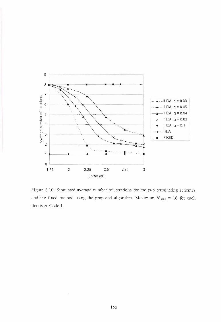
,_. *. -IHDA, q = 0.0011I·_·.··-IHDA, q =0.05

---..-IHDA, q =0.04

I ------?(--IHDA, q = 0.03

__ IHDA, q = 0.1

._.+.. - HDA

__FIXED

i------j

II1

-<''-.. , I-',.---,,---------'-'~

I-~- .-

~ - ---,:--",~,

\.___'. --"'I.", _

",,\.

9

8

en 7c0

ro 6m-'+-0 5L-

Cll..0

E 4::JC

Cll

W3Cll><{

2

-, .. __ .•........ -.

o1.75 2 2.25 2.5 2.75 3

Eb/No (dB)

Figure 6.10: Simulated average number of iterations for the two terminating schemes

and the fixed method using the proposed algorithm. Maximum NBDD = 16 for each

iteration. Code 1.

155

I-+-MAP Algorithm

,---.- Proposed Algorithm

43.532.521.50.5

100E-06 '----------------------'

o

1.00E-02

100E-05

100E+00

1.00E-04

wf«c::c::o 1.00E-03c::c::w,fro

Eb/No (dB)

Figure 6.11: Perfonnance companson of the trellis-based MAP algorithm and the

proposed algorithm for code 2. 8 iterations.

156

6.6 Conclusions

In this chapter, an efficient list-based decoding algorithm for GLD codes is proposed.

The decoding algorithm modifies and utilizes improved Kaneko's algorithm for soft

input hard-output decoding. In contrast to the improved Kaneko algorithm, three

modifications are introduced. First, list decoding is performed, i.e., all codewords

generated are stored. Secondly, a simple preprocessing test to avoid algebraic decoding

resulting in a codeword already found is proposed. This preprocessing test greatly

reduces the complexity of the proposed algorithm when compare to those used in [85],

[88], [89], [86]. Moreover, a method to generate soft-outputs is presented. To improve

the average decoding speed of the GLD decoder, two simple criteria for stopping the

iterative process for each frame immediately after the bits can be reliably decoded with

no further iterations are proposed.

Compared to the trellis-based MAP decoding algorithm, the proposed algorithm suffers

no degradation in performance at low bit-error rate, but has the additional advantages

that it can be used in cases where the trellis-based MAP algorithm would be

prohibitively complex and impractical. Compared to the Chase-based algorithm, the

proposed algorithm is more efficient, has lesser computational complexity for the same

performance, and provides an effective tradeoff between performance and

computational complexity to facilitate its usage in practical applications.

The proposed algorithm can easily be applied to different concatenated or compound

codes.

157

CHAPTER 7

UNION BOUND FOR BINARY LINEAR CODES ON THE

GILBERT-ELLIOTT CHANNEL MODEL WITH

APPLICATION TO TURBO-LIKE CODES

In this chapter, an analytical expression for the pairwise error probability of maximum

likelihood decoding of a binary linear code on the Gilbert-Elliott (GE) channel model is

derived. This expression is used to obtain the union bound on the bit error probability of

linear codes on the GE channel. Comparisons between the results obtained by this

analytical expression and results obtained through computer simulations in the case of

turbo codes and generalized irregular low density (GILD) codes show that the analytical

results are accurate in establishing the decoder performance in the range where


This chapter is organized as follows: A brief introduction to motivate the problem is

first presented. In Section 7.2, the GE channel model is described; some known

properties of the channel model are recapitulated, and useful statistical properties of the

chalmel are derived. Section 7.3 describes how the GE model can be matched to the

land mobile channel. In Section 7.4, the pairwise error probability on the GE channel is

derived, and this expression is used in Section 7.5 and Section 7.6 to obtain union

bound on the bit error probability of turbo codes and generalized irregular low density

(GILD) codes respectively. The simulation model and results are presented in Section

7.7, and finally conclusions are drawn in Section 7.8.

158

7.1 Introduction

It is well known that the real-world communication channel has memory, often

introducing noise distortion in a bursty fashion. In order to study the performance of

error correcting codes for such a channel, it is sometimes practical to use a model whose

properties are both complex enough to closely capture the real channel statistical

characteristics and simple enough to allow mathematically tractable system analysis.

For a channel with memory, the Gilbert-Elliott (GE) channel, which emerges from the

early 1960's and is due to Gilbert [101] and Elliott [102], is a useful and one of the

simplest discrete models that has been studied in considerable detail in the literature. In

this model, for a slowly varying channel, the channel is assumed to either be in a good

state, where the probability of error is small, or in a bad state, where the probability of

error is significantly larger. The dynamics of the channel are modelled as a first-order

Markov chain, a model which Wang and Moayeri [103] and Wang and Chang [104], in

spite of its simplicity, showed to be very accurate for a Rayleigh fading channel. In

[105], Ahlin presented a way to match the parameters of the GE model to the land

mobile chalmel, an approach that was generalized in [103] to a Markov model with

more than two states. This approach was also used by Sharma et al. in [106] and [107]

where error trapping decoders are studied.

Elliott [102] first analyzed the performance of error-correcting codes on a GE channel

by establishing a series of recursions for P(m, n), the probability of m transmission

errors in a block of n symbols. Recently Yee and Weldon [108] presented a

combinatorial analysis for a simplified GE channel that replaced the recursions with

closed-form expressions. An altemate norirecursive teclmique for approximate

evaluation of P(m, n) on simplified GE channels has also been presented by

Wilhelmsson and Milstein [109] and by Wong and Leung [110]. These analyses

considered block-coded transmission and are useful when the elTor correcting capability

of the code is known.

159

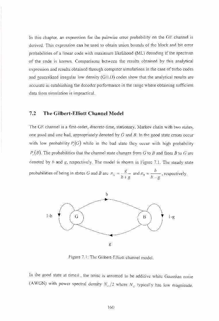
In this chapter, an expression for the pairwise error probability on the GE channel is

derived. This expression can be used to obtain union bounds of the block and bit error

probabilities of a linear code with maximum likelihood (ML) decoding if the spectrum

of the code is known. Comparisons between the results obtained by this analytical

expression and results obtained through computer simulations in the case of turbo codes

and generalized irregular low density (GILD) codes show that the analytical results are

accurate in establishing the decoder performance in the range where obtaining sufficient

data from simulation is impractical.

7.2 The Gilbert-Elliott Channel Model

The GE chmmel is a first-order, discrete-time, stationary, Markov chain with two states,

one good and one bad, appropriately denoted by G and B. In the good state errors occur

with low probability ~(G) while in the bad state they occur with high probability

p., (B). The probabilities that the channel state changes from G to B and from B to G are

denoted by band g, respectively. The model is shown in Figure 7.1. The steady state

probabilities of being in states G and Bare JrG =-g- and JrB = _b_, respectively.b+g b+g

l-b

g

l-g

Figure 7.1: The Gilbert-Elliott channel model.

In the good state at time k , the noise is assumed to be additive white Gaussian noise

(AWGN) with power spectral density N()2 where N G typically has low magnitude.

160

Similarly, in the bad state, the noise is white Gaussian with power spectral density

Nu l2 where NB > Nc ·

Figure 7.2 is useful in interpreting the significance of the two ,states. It shows the

received SNR, r, vs. time. If the SNR drops below some pre-determined threshold rT'

then the channel goes into the bad state else it resides in the good state. In either state,

the channel exhibits the properties of a binary symmetric channel. Figures 7.3 and 7.4

show the channel bit error characteristics in the two states respectively. In the bad state,

the probability of error is P"(B) and in the good state the probability of error is P"(G).

NOlmally, P"(G)« P"(B).

rtSNR

Good Bad state Good

t

time

Figure 7.2: Physical interpretation of the states in the Gilbert-Elliott model.

161

1-~(G)

o~---------------::?'"' o

~(G)

~(G)

1..::::::..----------------'"1-~(G)

1

Figure 7.3: Good state binary symmetric channel.

1- ~(B)o~------------~ 0

~(B)

1 ..c:::....- ~

1- ~(B)

Figure 7.4: Bad state binary symmetric channel.

(7.1){I ,

Y=0,

Let T(G) and T(B) be the number of time units the channel spends in the good and bad

state respectively. Their averages, f(G) and f(B) , can be obtain as follows:

Assume the channel is in the good state and let

if the next transition IS from G to B

if the next transition IS from G to G

f(G) = E[T(G)J = E[ E[T(G)/ YJ]

=E[T(G) / Y =1JPr {Y = I} + E[T(G) / Y = 0JPr {Y = o}

=bE[T(G)/Y = IJ+(l-b)E[T(G)/Y = OJ

=b+(I-b)(l+E[T(G)J) .

Therefore

162

{I ,

X=0,

Likewise, assume the channel is in the bad state and let

if the next transition IS from B to G

if the next transition IS from B to B

f (B) = E[T( B)J = E[E[T(B)/ XJJ=E[T(B)/ X =1JPr{X = I} + E[T(B)/ X =0JPr{X = o}

= gE [ T (B) / X = 1J+ (1- g) E [T (B) / X = 0J= g +(1- g )(1 + E[T(B)J).

Therefore

1f(B)=E[T(B)J=-.

g

(7.2)

(7.3)

(7.4)

(7.5)

In words T(G) and T(B) are geometric random variables with parameter band g

respectively.

7.3 Matching the Gilbert-Elliott Channel Model to the Land Mobile

Channel

In this section the generative GE model is related to the analogue Rayleigh fading

model, where the correlation function is given by the zeroth-order Bessel function, a

model commonly used for the land mobile channel, e.g. [111]. To do this, some results

concerning the memory of the analogue model are needed. As can be seen in Figure 7.5,

the signal envelope only occasionally experiences very deep fades. Shallow fades are

more likely to occur. A quantitative expression of this property is the level crossing rate,

h(), which is defined as the expected rate at which the envelope crosses a specified

threshold, rT' in the positive direction. If the SNR, r, is used instead of the signal

envelope level, R, the following expression for the level crossing rate is obtained [111],

h(r,) ~ 1")2,,~ exp(-r, IV),

163

where r T is the specified SNR threshold and r is the average SNR of the received

signal. The maximum Doppler shift, ID' is given by

ID =V/A, (7.6)

where v is the velocity of the moving vehicle and A is the carrier wavelength. Related

to the level crossing rate is the expected duration of the fade below the specified

threshold, r T' which is given by:

(7.7)

I

---I

10

1

0::: 0.1zCl) 0.01

0.001

0.00010 200 400 600 800 1000 1200 1400 1600 1800 2000

Time(in channel symbols)

Figure 7.5: An example of the received signal envelope on a typical simulated Rayleigh

fading (I,,, =0.001).

In (7.7), pr [r s Yr] represents the fraction of time the Rayleigh fading channel is below

Yr and is given by:

(7.8)

where /(r) is the distribution of the received SNR. It should be noted that the Rayleigh

fading results in an exponentially distributed multiplicative distortion of the signal. As a

result, the probability density function of the signal-to-noise ration (SNR), r, is given

by:

164

f(r)= ~exp(-r/r),r~O.r

Substituting (7.9) into (7.8) we obtain

pr [r ~ rT ] = 1- exp(- p ) ,

(7.9)

(7.10)

where p = r T / r .So the expected fade duration in a Rayleigh fading environment is

(7.11)

In the same way, the average non-fade duration E[r g] above the threshold is given by

1=-----==fD~2Jrp .

(7.12)

We want to relate the discrete channel model to the analogue one in such a way that the

discrete model should generate approximately the same error distribution as the

analogue channel (including the modulator and the demodulator). A natural way to

match the two models is to relate the state sequence to the fading signal envelope. Let

the bad state represents the situation when the signal envelope is below some threshold

and let the good state represents the situation when the signal envelope is above the

threshold. We then let the average number of time units the channel spends in the Good

(Bad) states be equal to the expected non-fade (fade) duration, normalized with the

symbol time-interval Ts '

f(G)=E[rgJ; ,s

f(B) =E[rh ]_1 .Ts

Hence, the transition probabilities are given by:

b = fj)1'.~)27[p ,

and

g = ,0)1'., /hP .exp(p) -1

165

(7.13)

(7.14)

(7.15)

(7.16)

The next step is to calculate the error probabilities in each state. They are taken to be the

conditional error probabilities of the Rayleigh fading channel, conditioned on being in

the respective state, i.e.

and

~(B)=_l rrr f(y)P(y)dy,7T: Jo

8

(7.17)

(7.18)

where p(y) is the symbol error probability for a given value of r, which depends on

the modulation format used. For BPSK modulation with coherent demodulation, the

conditional probability of a code symbol error, conditioned on the received SNR, is

given by [112]

~ (y) = ~erfc( fY),

where erfc(x) = ]-; rexp(- e~t is the complementary error function.

(7.19)

Substituting (7.9) and (7.19) into (7.17), the probability of error in the bad state, Pc(B)

IS

r~erfc(JY)~ exp(-rFf)drP (B)= 2 r

c Ir-=exp(-r/Y)drr

fYT1(f oo

2 (2)) 1 I_ 0"2 JYJ;exp -t dt yexP(-Ylr) dr

exp (- r / r) I~T

(7.20)

The integral, I, in the numerator defined as

(7.21)

can be evaluated by re'sorting to integration by parts.

166

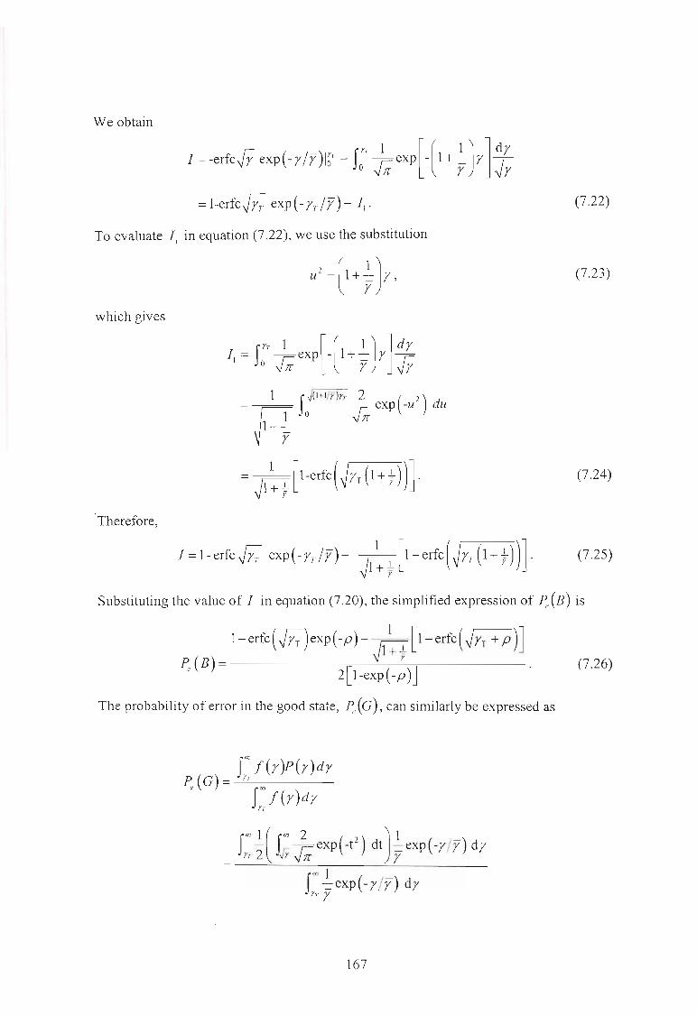
We obtain

kerfc'[y exp(-rjr)I:' - J:' );eX{(l+ ~)r]1r=l-erfcjY; exp(-rT/r)- 1,.

To evaluate 11

in equation (7.22), we use the substitution

which gives

fY1' 1 [( 1)] drJ1

= - exp - 1+-= r -o j; r JY

1 fJ(I+IIY)y, 2 (2 )= -exp -u du

~I+ ~ 0 Jff

.Therefore,

(7.22)

(7.23)

(7.24)

J =l-erfcF: exp(-r,jr) - A[1-erfC(Jr, (I +y))l (7.25)

Substituting the value of J in equation (7.20), the simplified expression of ;:'(B) is

I-erfc(F:)exp(-p)-A[1-erfcUrT +p )]

~(B)= 2[1-exp(-;)] (7.26)

The probability of error in the good state, Pe(G), can similarly be expressed as

fa) f(r)P(r)drPe (G) = -.-:.Y-,---1'-a)---

L,f(r)dr

_s:Hf;,-j;exp(-t') dt)~exp(-rjr) dr

fa) ~exp(-r/r) drY1' r

167

~I2 2

= exp(-Yrlr)'

where

12 = J"'(I'" ~exp(-t2) dtJ ~exp(-rlr) dr·Y1 JY -v Jr r

12can also be integrated by parts as was done for I yielding

12 = -erfcJY exp(-rIr) I; - J'" ~ exp[-(1+t )rJ dr::1 Y7" -V Jr \I r

c- 1 J'" 2 ?=erfc\lYr exp(-rTlr)-R I~) ,exp(-u-)du1+ -1 \/\1+ Yr}YT -V Jr

Y

Hence, ;:(C) can be expressed in the following form:

7.4 Pairwise Error Probability on the Gilbert-Elliott Channel

(7.27)

(7.28)

(7.29)

(7.30)

In this section we derive the expression of the pairwise ML decoding error probability

on the GE channel for two codewords/paths in a code trellis which differ in d symbols

when the channel state is known exactly to the decoder. If the channel state is known

exactly to the decoder we assume that amongst the d bits in which the wrong path and

the correct path differ, there are d a in the bad state and de = d - da in state C.

Amongst the bits in the bad state, there are ea bits in error and amongst the "good" bits

ee are in error. Let CM(I) and CM(O) be the likelihood metric of the wrong path and the

correct path respectively, restricted over the d positions in which the two paths differ;

CM(I) = eR log(l-;: (B)) +(dR -eR )log;: (B)

+ee 10g(1-;: (G) )+(de -ee )log~ (G)'

168

(7.31)

and

CM(O) = (dB -eB)log(1- ~ (B)) + eBlog~ (B)

+(de -ee)log(l-~(G))+ee log~(G)(7.32)

The probability of error in the pairwise comparison of the likelihood metrics CM(I) and

CM(O) is:

P2 (d) = Pr(CM(I) > CM(O)). (7.33)

If both metric values are equal, a random choice is made with probability 1/2. If

equations (7.31) and (7.32) are substituted into (7.33) we obtain:

where C is the metric ratio defined as

C = log [(1-~ (B)) / ~, (B)]log[(l-~(G))/~(G)J .

(7.34)

(7.35)

To evaluate P2(d), the probability distribution for being in the bad state dB times out of

d and the distribution for being in the good state de times out ofd is needed. It is

shown in Appendix C that

( )d-I

1-b 1[e' dB =0

[~I (dB/GG)+ ~I (dB/GB)J1[(; +[~I (dB/ BG)+ ~I (dB / BB)J1[B,l ~ dB < d

( )d-I

l-g 1[B'

(7.36)

where

(7.37)

(7.38)

(7.39)

(7.40)

169

Here, pAdB IGG) is the conditional probability of being dB times in the bad state,

conditioned on being in the good state both the first and the last instants of time. The

other probabilities are defined accordingly.

Following the same reasoning, it is easy to show that,

(l-g)d-'1rB

, dc=O

~I (dc;) = [~I (dci IGG)+ P" (dci 1GB )J1rCi + [~I (dci IBG) + P" (dci IBB)J1rH,l :-:; dc; < d

(l-b)"-I 1rC ' dc=d

(7.41)

where

1'" (d,)GG) ~ mi"ht,d,,·'t ~ ~G2-ldiG_~I)(1-b)',,-i bi-' (1- gt''' .. gi-i ,

Pd

(d,)GB) ~ mi"(d~_d"t~~Gl-ldt_~I)(I-b)',,-i bi(1-gt,,,-i g'-' ,

1'" (d,)BG) ~ mi"('~_d") (d -i~~ -ItiG_~ I)(1- b)',,-i bi' (1- gt,,,-i gi ,

1'" (d,) BB) ~ mi"(d'~d-d") ( d -i~Gl-l~c~~I} 1-bj"'-i" bi-' (1- gt',,-i gi-' ,

Thus

(7.42)

(7.43)

(7.44)

(7.45)

In (7.46), the summation over eB and ec is restricted to those values eB and ec which

fulfil the inequality in (7.34) and the factor 1/2 is introduced in case of equality. This

expression can be used to compute the union bound on the word and bit-error

probability of linear codes with maximum-likelihood decoding on the GE channel. In

the next two sections, it is applied to turbo codes and generalized irregular low density

(GILD) codes respectively.

170

7.5 Application to Turbo Codes

Since its introduction in 1993 by Berrou et al. [4], [5] turbo coding has raised great

interest in the communication community. A turbo encoder is formed by two parallel

concatenated recursive convolutional encoders connected by an interleaver. The

interleaver performs permutation of the input sequence. The decoder consists of two

iterative maximum-a-posteriori (MAP) decoders connected by an interleaver and

deinterleaver. Turbo codes have excellent bit error rate (BER) performance at low

SNRs. Performance near Shannon capacity limit can be obtained with large interleavers,

and comparatively good performance is possible for any interleaver size. However, at

high SNR, a flattening phenomenon of the BER curves has been observed [113]. This is

called the "error floor" of turbo codes. It is believed that the "error floor" is caused by a

small minimum distance. In general, it is very difficult to characterize the behaviour of

the "error floor" using simulation (the computational cost is too high). Instead, one

resorts to theoretical bounds. Many researchers have studied performance bounds for

turbo codes [113]-[118], [73], [78]. Although these works are studied on AWGN

channels, performance analysis of turbo codes over fading channels have also been

investigated [119], [120]. More recently, Kang et al. [121] and Garcias-Frias and

Villasenor [122] considered the design and performance of turbo codes on a GE channel

and proposed the necessary modifications to the turbo decoder. No analytical work on

the BER was done in these papers.

In this section, using the expression of the pairwise error probability derived in the

previous section, an expression for the union bound on the bit error probability of turbo

codes on the GE channel is obtained. With the assumption of uniform interleaver (a

collection of deterministic interleavers, each of which occurs with equal probability),

the key of union bound analysis of turbo codes largely depends on the weight

enumerating function (WEF) of the constituent codes. Although Benedetto et al. were

the first to introduce the concept of a unifonn interleaver, their method of calculating

the WEF is not accurate and not straightforward to comprehend. Divsalar et al. [116]

presented a recursive method, based on the transfer function method [123], to obtain the

WEF. Consider the traditional union upper bound for the ML decoding of a (N,K)

171

block code. Without loss of generality, it is assumed that the all-zeros codeword was

sent. The expression for the average bit error probability for the two constituent rate 1/2

convolutional codes is given by [116]

(7.47)

In (7.47), P2 (d) is the probability of incorrectly decoding a codeword with weightd ,

M = 3N , N being the input block length and d = i + d] + d2 • To calculate the

expression of equation (7.47), the distribution of the parity sequences d l and d 2 IS

required. This distribution can be given by [116]

(.)_ t(N,i,dp ) _ t(N,i,dp ) {}

Pdp/l -" (. )- (NJ ,pE 1,2L. t l,l,dpdfl .

1

(7.48)

where t(l, i, d p ), which can be found from the code's transfer function, is the number of

paths of length I , input weight i , and output weight d p' starting and ending in the all

zero state. With P(dp / i), the performance of turbo codes can be studied on various

statistical channels by formulating the two-codeword probability P2 (d) for the channel

of interest and using (7.47). For the GE channel, P2 (d) is given by equation (7.46).

7.6 Application to GLD Codes

GLD codes independently introduced by Lentmaier [55] and Boutros [56] were

presented in the previous chapter. In this section, using the expression of the pairwise

error probability derived in Section 7.4, an expression for the union bound on the bit

error probability of GLD codes on the GE channel is obtained.

7.6.1 Average Weight Distribution of GLD Codes

The direct computation of the exact weight distribution of a GLD code becomes rapidly

intractable when the length of the code N increases. The average weight coefficients of

a GLD code can be easily obtained by averaging over all the possible interleavers 7r ..J

172

Let us denote by g(s) the moment generating function of the component code, which is

the exponential polynomial whose coefficient gi of degree i is the normalized number

of codewords with weight i. As the J super-codes C. of length N are the direct sum of1

N / n independent constituent codes Co, their moment generating function Gc. (s) areJ

simply a power ofg(s):

Gc (s) = g (s )NIn = IQ (I) els,

II

(7.49)

where Q(l) is the probability that a codeword of C i has weight I. We assume without

loss of generality that all super-codes are built from the same constituent code. Since the

total number of codewords in C i is (2 k tin, the number of codewords of Ci

having

weight I is:

(7.50)

Thanks to the fact that CI"", CJ are randomly permuted versions of the same super

code, and thus independent, the probability p(l) that a vector of weight I belongs to

C = Cl n···nCJ , is the product of the probabilities that it belongs to each code:

(7.51)

Finally, the average number of codewords in C having weight I is:

(7.52)

Only GLD codes with two levels are considered for three major reasons. First, it was

shown that GLD codes with only J = 2 are asymptotically good [55], [56], [66].

Second, two levels is the best choice in terms of rate, as it decreases with J(6.1). Third,

the structure, graphical representation and decoding are simpler.

173

7.6.2 Union Bound on the Bit-Error Probability of GLD Codes on the GE

Channel

The average weight distribution of GLD codes (7.52) can be used for computing the

average bit error probability of ML decoding of GLD codes on various statistical

channels by formulating the two-codeword probability for the channel of interest.

Actually, the interleaver acts on all coded bits, so that they are equally protected. Thus

we obtain the following Union-Bound (UB) for transmission over the GE channel:

- N d --J:bsI-xN(d)xP2(d), (7.53)

d=l N

where P2 (d) is given by equation (7.46).

7.6.3 GLD Decoder for the Gilbert-Elliott Channel

The decoding of GLD codes is based on iterative soft-input soft-output (SISO) decoding

of individual constituent codes. In this chapter, only low rate GLD codes are

considered. Hence, exploiting the fact that the constituent code usually has a small code

length and high code rate, a trellis-based algorithm can be used to obtain high error

correcting performance with reasonable decoding complexity. In our implementation,

we used the trellis-based MAP (maximum a posteriori probability) algorithm [40], also

referred to as BCJR, on the syndrome trellis of the constituent code. The algorithm was

summarized in Chapter 4.

The modification of the GLD decoding algorithm for the Gilbert-Elliott channel is

dependent on what information is available to the GLD decoder. In this chapter, we

only consider the case of known channel state. If the state, G or B, is known, then the

modification to the GLD decoder is straightforward. Equations (4.87), (4.88), and (4.89)

still apply for the decoding of the component codes, where the relevant channel

reliability factor is given by:

L = 4E, { }c iEG,B.

N,

174

(7.54)

7.7 Simulation Model and Numerical Results

For all simulation and numerical results on turbo code, the component encoders are rate

one-half, recursive systematic convolutional encoders with memory two (four states)

and octal generators (7,S). The frame size is N = 1024 bits unless otherwise specified.

Perfect side information is assumed and the MAP algorithm is used as decoding

algorithm with the branch transition probabilities modified accordingly [121]. A two

level GLD code oflengthN = 420, rateR = 0.467, built from the (15,11,3) Hamming

code is considered. In order to represent a wide range of mobile communication

environments, the product fD~ was considered as an independent parameter /,,, and

numerical analysis and simulations were performed for /,,, = 0.1, and 0.03. Unless

otherwise specified, the signal-to-noise ratio threshold on the GE channel was set to 0.1

so that a SNR of 10 dB below the average SNR represents the transition to the bad state.

In Figure 7.6, the bound on the bit error rate of turbo code is evaluated for the above

values of the normalized Doppler frequency and for various block lengths. It can be

noticed that the bound diverges at low SNR. This behaviour mimics that of similar

bounds applied to totally random codes, which turbo codes resemble. This divergence is

an artifact of the bound, as the actual performance of the system does not diverge at low

SNR. In computing these bounds, we realized that only a handful of terms

i :s; 10, cl p :s; 20 are needed for convergence, and that this is almost independent of both

the values of the frame size N and the normalized Doppler frequency /,,, . In Figure 7.7,

the effect of the threshold on the accuracy of the bound is assessed. It can be observed

that a minor variation in this parameter does not dramatically affect the accuracy of the

bound. A comparison of the bound with simulated results in Figures 7.8 and 7.9

confimls the accuracy of the former at medium to high SNR. Thus the bound can be

used to predict the system performance in the range where obtaining sufficient data

from simulations is impractical and hence to detennine the coding gain.

In Figures 7.10 and 7.11, we compare the bound and the simulation results for the GLD

code. It can also be observed again that the bound is accurate at medium to high SNR.

175

1.00E-05

1.00E-09

'.

""

" I

... .1

I

1---...---... i

'..J',. -. I' .

iII

I'!... " I" ',I

- - _. - - -~. - -.., '

-.---N=10

·---··N=100

--N = 1024

1.00E-11

1.00E-13

1.00E-03

1.00E-01

.0Cl.c 1.00E-07o"0C::Jo

CO

20161284

1.00E-15 '----------------------------'

oMean SNR (dB)

Figure 7.6: Bounds on the bit error rate of 1/3 rate turbo code for various block lengths

N, fill = 0.1 (lower group), andfm = 0.03 (upper group).

176

-------------_._------

1.00E-01

1.00E-03 -

1.00E-05

.00..

§ 1.00E-07 ~

-ac:Jo

CO 1.00E-09

--......-'i----

'. ,-'. \

",\. '

- - - -.-,'. \

'. \--. "_." .. - ~

.- ---.......... ---.... .

'. '-.... ..:.~.<". . ......,

,.... ....

1.00E-11

1.00E-13--- ... -Threshold = 8 dB

--Treshold = 10 dB

- -_.- Threshold = 12 dB,

"\~,,~ ..,..~

"''1:..\>.;, -\,

20161284

1.00E-15 L-===============- --..i

oMean SNR (dB)

Figure 7.7: Bounds on the bit error rate of 1/3 turbo code for various values of the

threshold, fill = 0.1.

177

0.1

0.001

1E-05

2~ 1E-07g<lJ

co 1E-09 -

1E-11

1E-13 ~ ..

1E-15

o

'-~-+- Iteration # 1

i-.-Iteration # 6

i--Bound I

4 8 12 16 20

Mean SNR (dB)

Figure 7.8: Transfer function bound versus simulations results for 1/3 rate turbo code,

fill = 0.1.

178

0.1

0.001 ~.

1E-05(])

"§....e....(]) 1E-07......co

1E-09

1E-11 -+--Iteration # 1

----.-Iteration # 61

-Bound

1E-13

o 4 8 12

Mean SNR (dB)

16 20 24

Figure 7.9: Transfer function bound versus simulation results for 1/3 rate turbo code,

fill = 0.03.

179

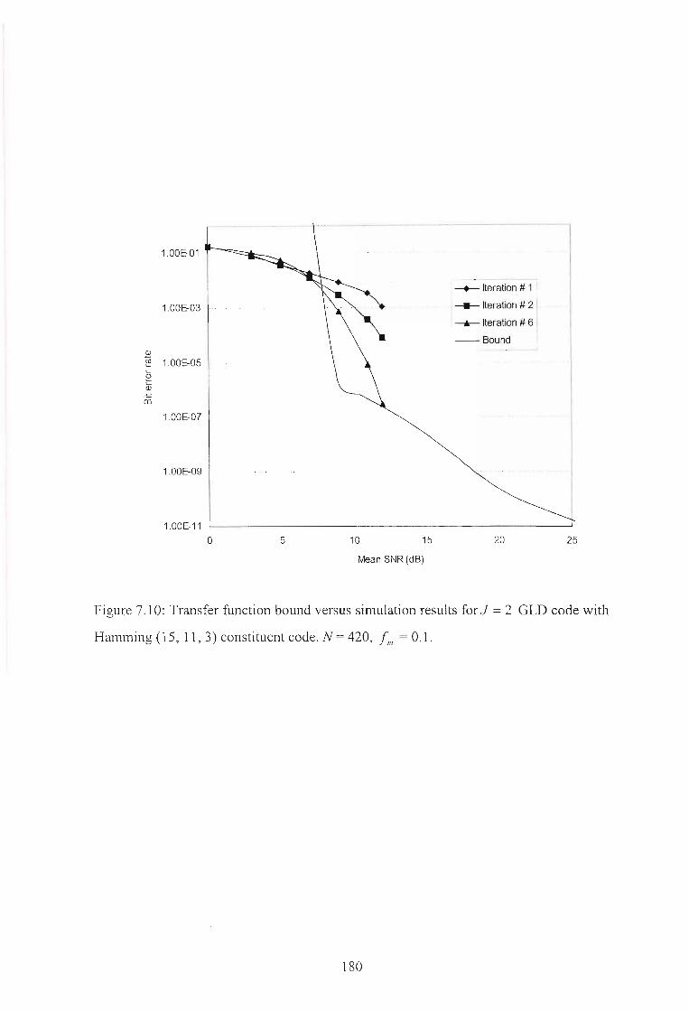
100E-01

1.00E-03

ID

"§ 1.00E-05~

ew

1.00E-07

1.00E-09

1.00E-11

o 5 10 15

,-+- Iteration # 1 '

. !--- Iteration # 21'---.- Iteration # 6

--Bound

20

I

·1I!

I--- --i

I

1!

--I

II

25

Mean SNR (dB)


Hamming (15,11,3) constituent code. N= 420, fill = 0.1.

180

1.00E+00

1.00E-02

1.00E-04

IDroI-

I-

e 1.00E-06I-

ID......(lJ

1.00E-08

1.00E-10

r--------I--------..------.---.--.----.--.~

I - I

-+-- Iteration # 1I.---..- Iteration # 2 I

- Iteration # 6,

:-Bound

1.00E-12

o 5 10 15 20 25

Mean SNR (dB)

30 35 40


Hamming (15,11,3) constituent code. N= 420, fill = 0.03.

181

7.8 Conclusion

In this chapter, an analytical expression for the pairwise error probability of maximum

likelihood decoding of a binary linear code on the GE channel model is derived. This

expression can be used to obtain the union bound on the bit error probability of linear

codes with maximum-likelihood decoding on the GE channel. The expression is used to

obtain union bound for turbo codes and GLD codes on the GE channel. Comparisons

between the results obtained by this analytical expression and results obtained through

computer simulation showed that, in both cases, the analytical results are accurate in

establishing the decoder performance in the range where obtaining sufficient data from

simulation is impractical.

182

CHAPTERS

CONCLUSION

8.1 Summary

This thesis deals with the design of concatenated codes and decoding algorithms as well

as their characterization in fading channel.

Inspired by recent results showing that irregular structure improves performance, the

generalization of irregular LDPC codes, called GILD codes, is introduced. GILD codes

are both an adaptation of, and an attractive alternative to GLD codes. The high

flexibility in selecting the parameters of GILD codes and their better performances and

. higher rates make them more attractive than GLD codes and hence suitable for small

and large block length forward error correcting schemes.

Two new decoding algorithms for LDPC codes are proposed. The first algorithm is a

hard-decision method, and the second one is a modification of the first to include

reliability information of the received symbols. In principle and in complexity, the

algorithms belong to the class of so called bit flipping algorithms. The defining attribute

of the proposed algorithms is the bit selection criterion which is based on the fact that,

for low density matrices, the syndrome weight increases with the number of errors in

average until error weights much larger than half the minimum distance. A loop

detection procedure with minimal computational overhead is also proposed that protects

the decoding from falling into infinite loop traps. Simulation results show that the

proposed algorithms offer an appealing performance/cost trade-offs.

Two new soft-input soft-output iterative decoding algorithms for compound codes

based on linear block codes are also proposed. The first algoritlun is based on MAP

decoding of low-weight subtrellis centered around a generated candidate codeword.

183

Simulation results indicate that the proposed algorithm provides a significant

improvement in error performance over Chase-based algorithm and achieves practically

optimal performance with a significant reduction in decoding complexity. The second

algorithm is a list based decoding algorithm. It modifies and utilizes the improved

Kaneko's decoding algorithm for soft-input hard-output decoding. These hard outputs

are converted to soft-decisions using reliability calculations. An important feature of

this algorithm is the derivation of a condition to rule out useless test error patterns in the

generation of candidate codewords. This rule-out condition reduces many unnecessary

decoding iterations and computations. Compared to the Chase-based algorithm, this

algorithm is more efficient, has lesser computational complexity for the same

perfonnance and provides effective tradeoff between performance and computational

complexity.

The characterization of linear codes in channel with memory is also investigated. An

analytical expression for the pairwise error probability of maximum likelihood decoding

of a binary linear code on a channel with memory modelled by the regenerative GE

chmmel model is derived. This expression is used to obtain the union bound on the bit

error probability of linear codes on the GE channel. Comparisons between the results

obtained by this analytical expression and results obtained through computer

simulations in the case of turbo codes, and GLD codes show that the analytical results

are accurate in establishing the decoder performance in the range where obtaining

sufficient data from simulation is impractical.

8.2 Future Work

Further investigations need to be carried out. It has been observed in Chapter 4 that, on

AWGN channel, there is a loss in a large range of SNR between the simulation results

for a fixed GILD code and the upper bound on the ML decoding error of the average

ensemble of GILD codes of the same length. It is well known that the interleaver is a

key component, which plays an important role in enhancing the performance of

compound codes. Future work should aim at designing appropriate interleavers for

GILD codes.

184

Another point that has not been studied is the encoding algorithm of GILD codes. As

with GLD codes, the parity check matrix is systematized to produce the associated

generator matrix. Even if the systematization is done offline once and that the encoding

complexity is not too high for small block length, this method is a drawback of GILD

codes and GLD codes compared to other compound codes for medium length. An

efficient encoding process taking account the graphical representation of GILD codes

may be found, to avoid the explicit construction of the generator matrix.

In Chapter 5, a new low-weight subtrellis based soft-input soft-output decoding

algorithm for linear block code suitable for iterative decoding is presented. This

algorithm can be improved in several ways. Furthermore a theoretical analysis of the

proposed algorithm and its complexity is to be studied. The two new decoding

algorithms for LDPC codes introduced in Chapter 3 can also be improved in several

ways.

Future research should also extend the work presented in Chapter 7 to derive improved

bounds that are accurate at low signal-to-noise ratio.

185

Appendix A

The MAP Algorithm for SPC Codes

Single parity-check (SPC) code is the simplest code together with the repetition code. If

it has length n, the code dimension is n -1 , and it its rate is R = (n -1)/ n . The nth bit is

parity bit, and it is computed by taking modulo 2 sum of all information bits. Maximum

a posteriori (MAP) decoding of an SPC code operates on log-likelihood ratios (LLRs)

of each received bit. Based on the received value corresponding to each bit, channel

LLRs are computed for each code bit position i, with O:s i < n :

(A.I)

MAP decoding algorithm computes the so-called extrinsic LLR for each bit. Expression

for the extrinsic LLR for code bit at position i is similar to the one for the channel LLR.

The difference is that probabilities are conditioned on all components of the received

sequence y, except the component Yi that corresponds to the ith code bit itself.

Consider first the case when we have only two information bits, Co and Cl' and parity

bit c2 • Then, c2 = Co EB Cl ' where EB indicates addition modulo 2. The extrinsic LLR for

Co is obtained as follows:

eL,(C,) + eL,(C,)= In ---,---1+ eL,(c,leL,(c,)

=-2 tanh -I ( tanh ( 1.,;(1»). tanh ( /" ~C'»))

The two last lines of (A.2) are obtained after some mathematical manipulation.

(A.2)

Extrinsic LLRs for bits Cl and c2 are obtained in the same way. For each bit, channel

LLR is improved by adding extrinsic LLR to it. Based on the sum

186

L (Cl) = Le (C; ) + Lex (c;) decision is made for bit c;. If L (c; ) > 0, the hard decision for

the ith bit is 1, Zi = 1, and if L (c; ) < 0, Zi = °.

Good approximation of the extrinsic LLR in (A.2) is given by the following expression:

The exact extrinsic LLR in (A.2) can be generalized to an SPC code of arbitrary length

n:

(AA)

The generalization of the approximation for extrinsic LLR given in (A.3) to an SPC of

length n is:

(A.S)

187

Appendix B

This appendix derives an upper bound on the Hamming distance between two distinct

codewords. For any two non equivalent error patterns, e(r) and eU) , define

z(r) = yH EB c(r) EB e(r) and zU) = yH EB c Ci ) EB eU). First we note that wH(z(r)):::; t and

wH (zCi)):::; t because of bounded distance decoding.

dH

(c(r) ,cU)) =dH

(z(r) EB e(r), zU) EB eU))

= wH

(z(r) EB e(r), zU) EB eel))

:::; wH

(e(r) EB il)) + wH

(z(r)) + wH

( z(J))

:::; d H (e(r) ,eel)) + 2t . (RI)

188

Appendix C

Derivation of Pd (d B) and Pd (dG) for the Pairwise Error Probability

Recall that we want to find the probability of being in state B exactly dB out of d times,

pAd IJ)' and the probability of being in state G exactly de out of d times, Pt! (de;)·

Consider Pt! (d IJ). For the cases d = 0 and d = n, the result is trivial, since d = 0 means

that the channel starts in the good state and never leaves it, which will happen with

probability (1- by-I 7t e , and d = n means that the channel starts in the bad state and

remains there, which will happen with probability (1 - gt l7t B. Henceforth, we may

therefore assume that I :s; d :s; n.

The channel behaviour can be depicted by one of the following four cases:

The channel starts in the good state and ends in the good state, which will

happen with probability pAdlJ/GG).

The channel starts in the good state and ends in the bad state, which will happen

with probability ~,(dH / GB).

The channel starts in the bad state and ends in the bad state, which will happen

with probability ~I (d H / BB).

The channel starts in the bad state and ends in the good state, which will happen

with probability ~l (d H / BG).

Pt! (d /j) is found by summing the conditional probabilities, weighted appropriately, i.e.

P" (d/j) = [p" (dH/GG) + Pt! (du/GB) ] !rei + [p" (d/j/BG) + P" (dlJ / BB)J!rH

. (C.I)

Now, consider P,,(dH/GG), and let i be the number of sojourns in the good state. The

number of sojourns in the bad state is then i-I. If the channel is in the bad state exactly

dB out of d times, then it is in the good state exactly d-dB. Clearly i:S; d - dB' otherwise

the channel would be in the good state too many times, and i-I :S dB' otherwise the

189

channel would be in the bad state too many times. The probability, apart from dB and d,

depends on the number of times the channel state changes, not on the exact behaviour of

the channel. In this case, we will have:

i-I transitions from a good state to a bad state, each of which will happen with

probability b.

d-dB-i transitions from a good state to a good state, each of which will happen

with probability I-b.

i-I transitions from a bad state to a good state, each of which will happen with

probability g.

dB-i+ 1 transitions from a bad state to a bad state, each of which will happen with

probability I-g.

The probability for this specific channel behaviour is given by:

(C.2)

Now, since the number of ways dB can be expressed as a sum of i-I positive intergers is

(C.3)

and the number of ways that d-dB can be expressed as a sum of i positive integers is

(CA)

we have that

By usmg similar arguments, it is straightforward to derive the other conditional

probabilities, and hence Pd (d R ), which concludes the proof.

~J (d(;) is also derived similarly.

190

References

[1] C. E. Shannon, "A Mathematical Theory of Communication," Bell System

Technical Journal, 1948.

[2] R. G. Gallager, Low-density parity-check codes, Cambridge, MA USA, MU

Press, 1963. Also available online at http://justice.mit.edulpeople/pubs/ldpc.ps.

[3] R. G. Gallager, "Low-density parity-check codes," IRE Trans. On Information

Theory, vol. 8, no. 1, pp. 21-28, Jan. 1962.

[4] C. Berrou, A. Glavieux, and P. Thitimajishima, "Near Shannon limit error

correcting coding and decoding: Turbo codes," in Proc. 1993 Int. Con! on

Communications, pp. 1064 -1070.

[5] C. Berrou and A. Glavieux, "Near optimum error correcting coding and

decoding: Turbo codes," IEEE Trans. Commun.. vol. 44, pp. 1261-1271, Oct.

1996.

[6] V. Zyab10v and M. Pinsker, "Estimation of the error-correction complexity of

Gallager low-density codes," Problemy Peradachi Informatsii, vol. 11, pp. 23

26, Jan. 1975.

[7] G. A. Margulis, "Explicit construction of graphs without short cycles and low

density codes," Combinatorica, vol. 2, no. 1, pp. 71-78,1982.

[8] R. M. Tanner, "A recursive approach to low complexity codes," IEEE Trans.

Inform. Theory, vol. 27, pp. 553-547, Sept. 1981.

[9] M. Sipser and D. A. Spielman, "Expander codes," IEEE Trans. Inform. Theory,

vol. 46, no. 6, pp. 1710-1722, Nov. 1996.

191

[10] D. J. C MacKay and R. M. Neal, "Near Shannon limit performance of low

density parity-check codes," Electronics Letters, vol. 32, pp. 1645-1646, Aug.

1996.

[11] N. Wiberg, Codes and Decoding on General graphs, PhD thesis, Linkoping

University, S-581 83, Linkoping Sweden, 1996.

[12] N. Sourlas, "Spin-glass models as error-correcting codes," Nature, vol. 339, pp.

693-695, June 1989.

[13] 1. Kantor and D. Saad, "Error-correcting codes that nearly saturate Shannon's

bound," Phys. Rev. Lett., vol. 83, pp. 2660-2663, 1999.

[14] D. J. C. MacKay, "Good Error-Correcting Codes based on Very Sparse

Matrices," IEEE Trans. Inform. Theory, vol. 45, no. 2, pp. 399-431, Mar. 1999.

[15] J. Peral, "Fusion, propagation, and structuring in belief networks," Artif. Intell.,

vol. 29, pp. 241-288, 1986.

[16] M. Luby, M. Mitzenmacher, M. A. ShokroUahi, D. A. Spielman, "Improved low

density parity-check codes using irregular graphs and belief propagation," in

Proc. International Symposium on Information Theory (ISIT'98), p. 117, Aug.

16-21, 1998. Also available online at

http://www.icsi.berkerly.edu/luby/PAPERS/belerr.ps.

[17] M. Luby, M. Mitzenmacher, M. A. Shokrollahi, D. A. Spielman, "Analysis of

low-density codes and improved designs using irregular graphs," Proc. Of the

30th

ACM STOC, May 23-26, 1998. Also available online at

http://www.icsi.berkerly.edu/luby/PAPERS/anaerr.ps.

192

[18] M. Luby, M. Mitzenmacher, M. A. Shokrollahi, D. A. Spielman, "Improved low

density parity-check codes using irregular graphs," IEEE Trans. Inform. Theory,

vol.47,no.2,pp.585-598,Feb.2001.

[19] T. Richardson, A. Shokrollahi and R. Urbanke, "Design of capacity-approaching

irregular low-density parity-check codes," IEEE Trans. Inform. Theory, vol. 47,

no.2,pp.619-637,Feb.2001.

[20] D. J. C. MacKay, S. T. Wilson, M. C. Davey, "Comparison of constructions of

irregular Gallager codes," IEEE Trans. Comm, vol. 47, pp. 1449-1454, Oct.

1999.

[21] S. -Y. Chung, G. D. Forney, T. J. Richardson, and R. Urbanke, "On the design

of low-density parity-check codes within 0.0045 dB of the Shannon limit," IEEE

Comm. Letters, vol. 5, no. 2, Feb. 2001.

[22] Y. Kou, S. Lin, and M. Fossorier, "Low-density parity-check codes based on

finite geometries: a rediscovery and new results," IEEE Trans. Inform. Theory,

vol. 47, no. 7, pp. 2711-2736, Nov. 2001.

[23] W. W. Peterson and E. J. Weldon, Jf., Error-Correcting Codes, 2nd ed., MIT

Press, Cambridge, MA., 1972.

[24] S. Lin and D. 1. Costello, Jf., Error Control Coding: Fundamentals and

Applications, Prentice Hall, Englewood Cliffs, New Jersey, 1983.

[25] H. Tang, 1. Xu, Y. Kou, S. Lin, and K. Abdel-Ghaffar, "On algebraic

construction of Gallager and circulant low-density parity-check codes," IEEE

Trans.Inform. Theory,vol. 50,no.6,pp. 1269-1279,June.2004.

[26] H. Tang, J. Xu, S. Lin, K. Abdel-Ghaffar, "Codes on finite geometries," accepted

for publication.in IEEE Trans. Inform. Theory, 2004.

193

[27] R. M. Tanner, D. Srkdhara, and T. Fuja, "A class of group-structured LDPC

codes," Proc. ofISTA 2001, Ambleside, England, 2001.

[28] 1. Djurdjevic, J. Xu, K. Abdel-Ghaffar, and S. Lin, "Construction of low-density

parity-check codes based on Reed-Solomon codes with two information

symbols," IEEE Commun. Lett., vo!. 7, no. 7, pp. 317-319, July 2003.

[29] V. D. Kolesnik, "Probability decoding of majority codes," Prob. Peredachi

Inform., vo!. 7, pp. 3-12, July 1971.

[30] Y. Kou, S. Lin, and M. P. C. Fossorier, "Low-density parity-check codes based

on finite geometries: A rediscovery and new results," IEEE Trans. Inform.

Theory, vo!. 47, pp. 2711-2736, Nov. 2001.

[31] Z. Liu and D. A. Pados, "A decoding algorithm for finite geometry LDPC

codes," submitted to IEEE Trans. Commun.

[32] F. R. Kschischang, B. J. Frey and H. -A. Loeliger, "Factor Graphs and the sum

product algorithm," IEEE Trans. Inform. Theory, vo!. 47, pp. 498-519, Feb.

2001.

[33] R. Lucas, M. Fossorier, Y. Kou, and S. Lin, "Iterative decoding of one-step

majority logic decodable codes based on belief propagation," IEEE Trans.

Commun., vo!. 48, pp. 931-937, June 2000.

[34] J. Pearl, Probabilistic Reasoning in Intelligence Systems: Netwroks ofPlausible

Inference, Morgan Kaufmann, San Mateo, 1988.

[35] M. Fossorier, M. Mihaljevic, and H. Imai, "Reduced complexity iterative

decoding oflow-density parity-check codes," IEEE Trans. Commun., vo!. 47, pp.

673-680, May 1999.

194

[36] 1. Chen and M. P. C. Fossorier, "Near optimum universal belief propagation

based decoding of low-density parity check codes," IEEE Trans. Commun., vol.

50, pp. 406-414, March 2002.

[37] 1. S. Reed, "A class of multiple-error-correcting codes and the decoding

scheme," IRE Trans., IT-4, pp. 38-49, Sept. 1954.

[38] D. E. Muller, "Application of Boolean algebra to switching circuit design and to

error detection," IRE Trans., EC-3, pp. 6-12, Sept. 1954.

[39] J. L. Massey, Threshold Decoding, Cambridge, MA: MIT Press, 1963.

[40] L. Bahl, J. Cocke, F. Jelinek, and J. Raviv, "Optimal decoding of linear codes for

minimizing symbol error rate", IEEE Trans. Inform. Theory, vol. IT-20, pp. 284

287, March 1974.

[41] T. Beth, D. Jungnickel, and H. Lenz, Design Theory, Cambridge, U.K:

Cambridge Univ. Press, 1986.

[42] B. Vasic and O. Milenkovic, "Combinatorial construction of low-density parity

check codes for iterative decoding," IEEE Trans. Inform. Theory, vol. 50, no. 6,

pp. 1156-1176, June 2004.

[43] B. Ammar, B. Honary, Y. Kou, J. Xu, and S. Lin "Construction of low-density

parity-check codes based on balanced incomplete block designs," IEEE Trans.

Inform. Theory, vol. 50, no. 6, pp. 1257-1268, June 2004.

[44] S. Lin, L. Chen, 1. Djurdjevic, 1. Xu, "Near Shannon limit quasi-cyclic low

density parity-check codes," in Proc. IEEE GlobeCom '2003, pp. 2030-2035, San

Francisco, CA, Dec. 2003.

195

[45] L. Chen, J. Xu, 1. Djurdjevic, and S. Lin, "Near Shannon limit quasi-cyclic low

density parity-check codes," IEEE Trans. Commun., vol. 52, no. 7, July 2004.

[46] G. A. Margulis, "Explicit construction of graphs without short cycles and low

density codes," Combinatorica, 2(1): 71-78, 1982.

[47] J. Rosenthal and P. O. Vontobel, "Construction ofLDPC codes using Ramanujan

graphs and ideas from Margulis," in Proc. The 38th Allerton Con! On Commun.,

Control and Computing, pp. 248-257, Monticello, IL, Octo 4-6, 2001.

[48] A. Lubotzky, R. Phillips, and P. Samak, "Ramanujan graphs," Combinatorica,

8(3):261-277,1988.

[49] P. Samak, Some applications of modular forms, Cambridge University Press,

Cambridge, 1990.

[50] X. Y. Hu, E. Eleftheriou, and D. M. Amold, "Progressive edge-growth Tanner

graph," IBM Research, Zurich Research Laboratory, 8803, Rlischlikon,

Switzerland.

[51] P. Erdos and H. Sachs, Regulare Graphen gegebener Taillenweite mit minimaler

Knotenzahl, Wiss. Z. Univ. Hall Martin Luther Univ. Halle-Wittenberg Math.

Natur. Reine, 12:251-257, 1963.

[52] D. A. Spielman, "Finding good LDPC codes," 36th Annual Allerton Conference

on Communication, Control, and Computing, 1998. http://www-

math.mit.edu/spielman/theory/research ecc.html.

[53] S. y. Chung, T. Richardson, and R. Urbanke, "Analysis of sum-product

decoding of low-density parity-check codes using a Gaussian approximation,"

IEEE Trans. Inform. Theory, vol. 47, pp. 638-656, Jan. 2000.

196

[54] T. Richardson, A. Shokrollahi, and R. Urbanke, "Design of provably good low

density parity-check codes, tech. Rep., Bell Labs, Lucent Technologies, Murray

Hill, NJ 07947, Apr. 1999.

[55] M. Lentmaier and K. Sh. Zigangirov, "On generalized low-density check codes

based on Hamming component codes," IEEE Commun. Left., vo!. 3, no. 8, pp.

248-250, August 1999.

[56] J. Boutros, O. Pothier, and G. Zemor, "Generalized low density (Tanner) codes,"

in Proc. ICC'99, Houston, July 1999.

[57] T. Richardson and R. Urbanke, "Efficient encoding of low-density parity-check

codes," IEEE Trans. Inform. Theory, vo!. 47, pp. 638-656, Feb. 2000.

[58] J. -F. Cheng and R. J. McEliece, "Some high-rate near capacity codecs for the

Gaussian channel," in 34th Allerton Con! Communications, Controls and

Computing, 1996.

[59] M. C. Davey and D. J. C. Mackay, "Low-density parity-check codes over

GF(q)," IEEE Commun. Left., vo!. 2, pp. 165-167, June 1998.

[60] T. Richardson and R. Urbanke, "The capcity of low-density parity-check codes

under message-passing decoding," IEEE Trans. Inform. Theory, vo!. 47, pp. 599

618, Feb. 2001.

[61] M. Luby, M. Mitzenmacher, M. A. Shokrollahi, D. A. Spielman, and V. Stemann

"Practical loss-resilient codes," in Proc. 29th Annu. Symp. Theory ofComputing,

1957, pp. 150-159.

[62] M. Luby, M. Mitzenmacher, M. A. Shokrollahi, D. A. Spielman, "Analysis of

random processes via and-or trees," in Proc. 9th Annu. ACM-SIAM Symp.

Discrete Algorithms, 1998, pp. 364-373.

197

[63] N. Wiberg, H. -A. Loe1iger, and R. K6tter, "Codes and iterative decoding on

general graphs," Euro. Trans. Telecommun., vo!. 6, pp. 513-526, Sept. 1995.


"Efficient erasure correcting codes," IEEE Trans. Inform. Theory, vol. 47, pp.

569-584, Feb. 2001.

[65] D. J. C. MacKay. (1998) Turbo codes are low-density parity-check codes.

Available on line at: http://www.cs.toronto.edu/~mackav/abstracts/-turbo

ldpc.html.

[66] O. Pothier, Compound codes based on graphs and their iterative decoding, Ph.D.

thesis, Ecole Nationale Superieure des Telecommunications, Jan. 2000.


"Practical loss-resilient codes," IEEE Trans. Inform. Theory, vo!. 47, pp. 569

584, Feb. 2001.

[68] FJ. MacWilliams, NJ.A. Sloane: The theory of error-correcting codes, North

Holland, Englewood Cliffs, eighth impression, 1993.

[69] E. R. Berlekamp: Algebraic Coding Theory, Aegean Park Press, Revised 1984

Edition.

[70] M. Abramowitz and 1. Stegun, Handbook of mathematical functions, Dover

publications !nc, New York, ninth printing, 1972, p. 257.

[71] A. J. Viterbi, J. K. Omura, Principles of digital communications and coding,

McGraw-Hill, 1979.

198

[72] R. G. Gallager, Information theory and reliable communication, John Wi1ey &

Sons, 1968.

[73] T. M. Duman, and M. Sahe1i, "New performance bounds for turbo codes," IEEE

Trans. Commun., vol. 46, no. 6, June 1998, pp. 717-723.

[74] E. R. Berlekamp, "The technology of error-correcting codes," Proceeding of the

IEEE, vol. 68, no. 5, pp. 564-593, May 1980.

[75] G. Poltyrev, "Bounds on the decoding error probability of binary linear codes via

their spectra," IEEE Trans. On In! Theory, vol. 40, no. 4, July 1994, pp. 1284

1292.

[76] H. Herzberg and G. Poltyrev, "The error probability of m-ary PSK block coded

modulation schemes," IEEE Trans. Commun., vol. 44, no. 4, April 1996, pp.

427-433.

[77] 1. Sason and S. Shamai (Shitz), "Bounds on the error probability ofML decoding

of block and turbo-block codes," Annales des Telecommunications, vol. 5, no. 3

4, Mars-April 1999, pp. 183-200.

[78] 1. Sason and S. Shamai (Shitz), "Improved upper bounds on the ML decoding

error probability of parallel and serial concatenated turbo codes via their

ensemble distance spectrum," IEEE Trans. On In! Theory, vol. 46, no. 1,

January 2000, pp. 24-47.

[79] A. Lafourcade and A. Vardy, "Asymptotically good codes have infinite trellis

complexity," IEEE Trans. on Inf. Theory, vol. 41, pp. 555-559, Mar. 1995.

[80] D. Chase, "A class of algorithms for decoding block codes with channel

measurement information," IEEE Trans. on In! Theory, vol. 18, pp. 170-182,

Jan. 1972.

199

[81] G. D. Fomey Jr., "Generalized minimum distance decoding," IEEE Trans. on

In! Theory, vol. 12, pp. 125-131, Apr. 1966.

[82] M. P. C. Fossorier and S. Lin, "Soft-decision decoding of linear block codes

based on ordered statistics," IEEE Trans. on In! Theory, vol. 41, pp. 1379-1396,

Sept. 1995.

[83] T. Kaneko, T. Nishijima, H. Inazumi, and S. Hirasawa, "An efficient maximum

likelihood-decoding algorithm for linear block codes with algebraic decoder,"

IEEE Trans. Inform. Theory, vol. 40, pp. 320-327, Mar. 1994.

[84] M. P. C. Fossorier and S. Lin, "Soft-input soft-output decoding of linear block

codes based on ordered statistics," Globecom, 1998.

[85] R. M. Pyndiah, "Near-optimum decoding of product codes: Block turbo codes,"

IEEE Trans. Commun., vol. 46, pp. 1003-1010, Aug. 1998.

[86] P. A. Martin and D. P. Taylor, "On adaptive reduced-complexity iterative

decoding," Proc. 2000 IEEE Global Telecomm. Conf. (GLOBECOM'OO), pp.

772-776, 2000.

[87] S. Lin, T. Kasami, T. Fujiwara, and M. Fossorier, Trellisses and trellis-based

Decoding Algorithm for Linear Block Codes, Kluwer Academic Publishers,

1998.

[88] A. Picart and R. Pyndiah, "Adapted iterative decoding of product codes," in

Proc. Globecom, 1999, pp. 2357-2362.

[89] P. A. Martin and D. P. Tay1or, "On multi1evel codes and iterative multistage

decoding," IEEE Trans. Commun., vol. 49, No. 11, pp. 1916-1925, Nov. 2001.

200

[90] T. Johanson and K. Zigangirov, "A simple one sweep algorithm for optimal APP

symbol decoding of linear block codes," IEEE Trans. Inform. Theory, vol. 44,

pp. 3124-3129, Nov. 1998.

[91] T. Kaneko, T. Nishijima, and S. Hirasawa, "An improvement of soft-decision

likelihood decoding algorithm using hard-decision bounded-distance decoding"

IEEE Trans. Inform. Theory, vol. 43, pp. 1314-1319, July. 1997.

[92] S. Dave, J. Kim and S. C. Kwatra, "An efficient decoding algorithm for block

turbo codes," IEEE Trans. Commun., vol. 49, pp. 41-46, Jan. 2001.

[93] T. Y. Hwang, "Decoding linear block codes for minimizing word error rate,"

IEEE Trans. Inform. Theory, vol. IT-25, pp. 733-737, Nov. 1979.

[94] G. D. Fomey, Jr., Concatenated codes (MIT research monograph no. 37).

Cambridge, MA: MIT Press, 1966.

[95] H. T. Moorthy, S. Lin, and T. Kasami, "Soft-decision decoding of binary linear

block codes based on an iterative search algorithm," IEEE Trans. Inform.

Theory, vol. 43, pp. 1030-1040, May 1997.

[96] J. Hagenauer, E. Offer, and L. Papke, "Iterative decoding of binary block and

convolutional codes," IEEE Trans. on Inf Theory, vol. 44, pp. 429-445, Mar.

1996.

[97] T. M. N. Ngatched and F. Takawira, "A simple stopping criterion for turbo

decoding," lEE Electronic Letters, vol. 37, no. 22, pp. 1350-1351, Get. 25, 2001.

[98] R. Y. Shao, S. Lin, and M. P. C. Fossorier, "Two simple stopping criteria for

turbo decoding," IEEE Trans. Commun., vol. 47, pp. 1117-1120, Aug. 1999.

201

[99] Yufei Wu, B. D. Woemer and W. J. Ebel, "A simple stopping criterion for turbo

decoding" IEEE Communications Letters, vol. 4, No. 8, pp. 258-260, August

2000.

[100] R. H. Morelos-Zaragoza, The art oferror correcting coding, First edition, Jolm

Wiley & Sons, 2002.

[101] E. N. Gilbert, "Capacity ofa burst-noise channel," Bell Syst. Tech. J, vol. 39, pp.

1253-1265, Sept. 1960.

[102] E. O. Elliott, "Estimates of error rates for codes on burst-noise channels," Bell

Syst. Tech. J., vol. 42, pp. 1977- 1997, Sept. 1963.

[103] H. S. Wang and N. Moayeri, "Finite-state Markov channel-A useful model for

radio communication channels," IEEE. Trans. Veh. Technol., vol. 44, pp. 163

171, Feb. 1995.

[104] H. S. Wang and P. C. Chang, "On verifying the first-order Markovian

assumption for a Rayleigh fading channel model," IEEE trans. Veh. Technol.,

vol. 45, pp. 353-357, May 1996.

[105] L. Ahlin, "Coding methods for the mobile radio channel," presented at Nordic

Seminar on Digital Land Mobile Communications, Espoo, Findland, Feb. 1985.

[106] G. Sharma, A. Dholakia, and A. A. Hassan, "Simulation of error trapping

decoders on a fading channel," in Proc. 1996 IEEE Vehicular Technology Coni,

Atlanta, GA, Apr. 28-May 1, 1996, pp. 1361-1365.

[107] G. Sharma, A. A. Hassan and A. Dholakia, "Performance evaluation of burst

error correcting codes on a Gilbert-Elliott channel," IEEE Trans. Comm. Vol. 46,

No. 7, July 1998.

202

[108] J. R. Yee and E. J. Weldon, "Evaluation of the performance of error-correcting

codes on a Gilbert Channel," IEEE Trans. Comm. Vol. 43, No. 8, August 1995.

[109] L. Wilhelsson and L. B. Milstein, "On the effect of imperfect interleaving for the

Gilbert-Elliott channel," IEEE Trans. Comm. Vol. 47, No. 5, pp. 681-688, May

1999.

[110] B. Wong and C. Leung, "On computing undetected error probabilities on the

Gilbert channel," IEEE Trans. Commun., vol. 43, pp. 2657-2661, Nov. 1995.

[111] W. C. lakes, Ed., Microwave Mobile Communications. New York: IEEE Press,

1974.

[112] J.G Proakis, Digital Communications. New York: McGraw-Hill, 1989.

[113] P. Robertson, "Illuminating the structure of code and decoder of parallel

concatenated recursive systematic (turbo) codes," in Proc. GLOBECOM 94, pp.

1298-1303, Dec. 1994.

[114] S. Benedetto and G. Montorsi, "Unveilling turbo codes: some results on parallel

concatenated coding schemes," IEEE Transactions on Information Theory, vol.

42, No. 2, pp. 409-428, March 1996.

[115] S. Benedetto and G. Montorsi, "Performance evaluation of turbo-codes,"

Electronics Letters, vol. 31, No. 3, pp. 163-165, Feb. 1995.

[116] D. Divsalar, S. Do1inear, F. Pollara and R. J. McEliece, "Transfer function

bounds on the performance of turbo codes," JPL TDA progress Reports, 42-122,

pp. 44-45, Aug. 1995.

[117] 1. Sason and S. Shamai (Shitz), "Improved upper bounds on the decoding error

probability of parallel and serial concatenated turbo codes via their ensemble

203

distance spectrum," Proceeding ofIEEE International Synposium on Information

Theory, p. 30, MIT, Cambridge, MA, USA, Aug. 1998.

[118] Y. V. Sirid, "Weight distributions and bounds for turbo codes," European

Transaction on Telecommunication and Related Technologies, vol. 6, No. 5, pp.

543-555, Sept. - Oct. 1995.

[119] E. K. Hall and S. G. Wilson, "Designing and analysis of turbo codes on Rayleigh

fading channels," IEEE Journal of Selected Area in Communications, pp. 160

174, Feb. 1998.

[120] J. Y. Kim, "Performance of OFDM/CDMA system with turbo coding in a

multipath fading channel," IEEE Trans. On Consumer Electronics, vol. 45, No.

2, pp. 372-379, May 1999.

[121] 1. H. Kang, W. E. Stark and A. O. Hero, "Turbo codes for fading and burst

channels," Proceedings of the Communications Theory Miniconference,

Globecom'99, pp. 40-45, Nov. 1998.

[122] 1. Garcias-Frias and J. D. Villasenor, "Turbo decoding of Gilbert-Elliott

channels," IEEE Trans. Commun., vol. 50, No. 3, pp. 357-363, Mar. 2002.

[123] R. J. McEliece, "How to compute weight enumerators for convolutional codes,"

Communications and coding, pp. 121-141, M. Damell and B. Honary, eds.

Tauton Sumerest, England: Research Studies Press Ltd., 1998.

[124] S. A. Barbulescu, Iterative decoding of turbo and other concatenated codes,

Ph.D. thesis, School of Electrical Engineering, Faculty of Engineering,

University of South Australia, Feb. 1996.

204

[125] E. K. Hall and S. G. Wilson, "Design and analysis of turbo codes for

noncoherent channels," in Proc. IEEE Communication Theory Mini-conference,

Phoenix, USA, Nov. 1997, pp. 66-70.

[126] P. Frenger, "Turbo decoding on Rayleigh fading channel with noisy channel

estimates," in Proc. IEEE VTC'99, Houston, TX, May 1999, pp. 884-888.

[127] O. Edfors, M. Sandell, JJ. Van de Beek, S.K. Wilson, and P.O. Brjesson,

"OFDM channel estimation by singular value decomposition," in Proc. IEEE

Vehicular technology Con!, Atlanta, GA, Apr. 28-May 1, 1996, pp. 924-927.

[128] J. K. Wolf, "Efficient maximum likelihood decoding of linear block codes using

a trellis," IEEE Trans. Inform. Theory, vol. IT-24, pp. 76-80, Jan. 1978.

[129] G. D. Fomey, Jr., "Coset codes II: Binary lattices and related codes," IEEE

Trans. Inform. Theory, vol. IT-28, pp. 1152-1187, Sept. 1988.

[130] A. Vardy and Y. Be'ery, "Maximum likelihood soft-decision decoding of BCH

codes," IEEE Trans. Inform. Theory, vol. 40, pp. 546-554, Mar. 1994.

[131] D. J. Muder, "Minimal trellises for block codes," IEEE Trans. Inform. Theory,

vol. 34, pp. 1049-1053, Sept. 1988.

[132] T. Kasami, T. Takata, T. Fujiwara, and S. Lin, "On the optimum bit orders with

respect to the state complexity of trellis diagrams of binary linear codes," IEEE

Trans. Inform. Theory, vol. 39, pp. 242-245, Jan. 1993.

[133] T. Kasami, T. Takata, T. Fujiwara, and S. Lin, "On complexity of trellis

structure of linear block codes," IEEE Trans. Inform. Theory, vol. 39, pp. 1057

1064, May. 1993.

205

[134] Y. Berger and Y. Be'ery, "Bounds on the trellis size of linear block codes,"

IEEE Trans. Inform. Theory, vol. 39, pp. 203-209, Jan. 1993.

[135] V. V. Zyablov and V. R. Sideroko, "Bounds on the complexity of trellis

decoding of linear block codes," Probl. Pred. Inform., vol. 29, July/Sept. 1993.

[136] T. Kasami, T. Takata, T. Fujiwara, and S. Lin, "On structural complexity of the

L-section minimal trellis diagrams for binary linear block codes," IEICE Trans.

Fundamentals of Elec., Comm. Comp. Sci., vol. E76-A, no. 9, pp. 1411-1421,

Sept. 1993.

[137] T. Kasami, T. Takata, T. Fujiwara, and S. Lin, "On branch labels of parallel

components of the L-section minimal trellis diagrams for binary linear block

codes," IEICE Trans. Fundamentals ofElec., Comm. Comp. Sci., vol. E77-A, no.

9, pp. 1058-1068, June. 1994.

[138] G. D. Fomey, Jr., "Dimension/length profiles and trellis complexity of linear

block codes," IEEE Trans. Inform. Theory, vol. 40, pp. 1741-1772, Nov. 1994.

[139] G. D. Fomey, Jr. and M. D. Trott, "The dynamics of group codes: State spaces,

trellis diagrams and canonical encoders," IEEE Trans. Inform. Theory, vol. 39,

pp. 1491-1513, 1993.

[140] A. Barg, E. Krouk, and H. C. A. van Tilborg, "On the complexity of minimum

distance decoding oflong linear codes," IEEE Trans. Inform. Theory, vol. IT-45,

pp. 1392-1405, July 1999.

[141] P. Robertson, P. Hoeher, and E. Villebrun, "Optimal and sub-optimal a posteriori

algorithms suitable for turbo decoding," European Trans. On

Telecommunications, vol. 8, no. 2, Mar-Apr. 1997, pp. 119-125.

206

[142] J. Hagenauer, E. Offer, L. Papke, "A viterbi algorithm with soft-decision outputs

and its applications," Proceedings of GLOBECOM'89, Dallas, Texas, pp.

47.1.1-47.1.7, Nov. 1989.

[143] S. M. Kay, Fundamentals of Statistical Signal Processing: Estimation Theory,

Prentice Hall, 1993.

[144] A. Papoulis, Probability, Random variables, and stochastic Processes, McGraw

Hill, 3rd edition, 1991.

[145] S. K. Wilson, Digital audio broadcasting in a fading and dispersive channel,

PhD thesis, Dept. of Electrical Engineering, Stanford University, Aug. 1994.

[146] A. Vardy and Y. Be'ery, "Maximum likelihood soft-decision decoding of BCH

codes," IEEE Trans. Inform. Theory, vol. 40, pp. 546-554, Mar. 1994.

[147] Y. Berger and Y. Be'ery, "Soft trellis-based decoder for linear block codes,"

IEEE Trans. Inform. Theory, vol. 40, pp. 764-773, May 1994.

[148] L. Ekroot and S. Dolinear, "A decoding of block codes," IEEE Trans. Commun.,

vol. 50, No. 9, pp. 1052-1056, Sep. 1996.

[149] Y. S. Han, C. R. P. Hartmann, and c.-C. Chen, "Efficient priority-first search

maximum-likelihood soft-decision decoding of linear block codes," IEEE Trans.

Inform. Theory, vol. 39, no. 5, pp. 1541-1523, Sep. 1993.

[150] A. Lafourcade and V. Vardy, "Optimum sectionalization of a trellis," IEEE

Trans. Inform. Theory, vol. 42, no. 3, pp. 689-702, May 1996.

[151] R. J. McEliece, "On the BCJR trellis for linear block codes," IEEE Trans.

Inform. Theory, vol. 42, no. 4, pp. 1072-1092, Jul. 1996.

207

[152] T. Koumoto, T. Takata, T. Kasami and S. Lin, "A low-weight trellis based

iterative soft-decision decoding algorithm for binary linear block codes," IEEE

Trans. Inform. Theory, vol. 42, no. 3, pp. 1072-1092, Mar. 1999.

[153] T. M. N. Ngatched and F. Takawira, "Decoding of GLD Codes in a Rayleigh

Fading Channel With Imperfect Channel Estimates," in Proc. South African

Telecommunication Networks & Applications Conference, Drakensberg, South

Africa, 1-4 Sept. 2002.

[154] T. M. N. Ngatched and F. Takawira, "Generalized Irregular low-Density

(Tanner) Codes based on Hamming Component Codes," in Proc. IEEE

AFRICON 2002, pp. 193-196, Octo 2002.

[155] T. M. N. Ngatched and F. Takawira, "Efficient Decoding of Generalized Low

Density Parity-Check Codes Based on Long Component codes," in Proc. WCNC

2003, IEEE Wireless Communications and Networking Conference, vo!. 4, no. 1,

pp. 705 - 710, Mar. 2003.

[156] T. M. N. Ngatched and F. Takawira, "Error-Correcting Codes Based on Irregular

Graphs," in Proc. South African Telecommunication Networks & Applications

Conference, George, South Africa, 8-10 Sept. 2003.

[157] T. M. N. Ngatched and F. Takawira, "A low-weight trellis based soft-input soft

output decoding algorithm for binary linear block codes with application to

generalized Irregular low-density codes," in Proc. GLOBECOM 2004, IEEE

Global Telecommunications Conference, vo!. 4, no. 1, pp. 705-71 0, Nov. 29

Dec. 3, 2004.

[158] T. M. N. Ngatched and F. Takawira, "An Iterative Soft-Input Soft-Output

Decoding Algorithm for Linear Block Codes," in Proc. South African

Telecommunication Networks & Applications Conference, Spier Wine Estate,

Western Cape, South Africa, 6-8 Sept. 2004.

208

[159] T. M. N. Ngatched and F. Takawira, "Pairwise error probability on the Gilbert

Elliott channel with application to turbo codes," in proc. IEEE AFRICON 2004,

pp. 279-284, Sept. 2004.

[160] T. M. N. Ngatched, M. Bossert, and A. fahrner, "Two decoding algorithms for

low-density parity-check codes," accepted for presentation at IEEE International

Conference on Communications (ICC) 2005, 16 - 20 May 2005, Seoul, Korea.

[161] T. M. N. Ngatched and F. Takawira, "Improved generalized low-density parity

check codes using irregular graphs," SAIEEE Transactions, vol. 94: pp. 43-49.

[162] T. M. N. Ngatched and F. Takawira, "High-performance low-complexity

decoding of generalized low-density (GLD) parity-check codes," submitted to

IEEE Trans. Commun., Aug. 2003.

[163] T. M. N. Ngatched and F. Takawira, "Generalization of irregular low-density

parity-check codes," submitted to IEEE Trans. Commun., Dec. 2003.

[164] T. M. N. Ngatched and F. Takawira, "Union bound for binary linear codes on the

Gilbert-Elliott channel with application to turbo-like codes," submitted to IEEE

Trans. Veh. Technol., June. 2004.

[165] T. M. N. Ngatched, M. Bossert, and A. fahrner, "Hard- and soft-decision

decoding algorithms for low-density parity-check codes," in preparation, to be

submitted to IEEE Trans. Commun.

[166] M. Bossert and F. Hergert, "Hard- and soft-decision decoding beyong the half

minimum distance - An algorithm for linear codes," IEEE Trans. Inform.

Theory, vol. IT-32, no. 5, Sept. 1986.

209

[167] M. Bossert, Channel coding for Telecommunications, Wiley, New York, 1999,

pp. 165-167.

[168] R. Lucas, M. Bossert, and M. Breitbach, "On Iterative soft-decision decoding of

linear binary block codes and product codes" IEEE J Select. Areas Commun.,

vol. 16, no. 2, pp. 276-296, Feb. 1998.

[169] X. Y. Hu, E. Eleftheriou, and D. M. Arnold, "Regular and irregular progressive

edge-growth Tanner graphs," IEEE Trans. Inform. Theory, vol. 51, no. 1, pp.

386-398, Jan. 2005.

[170] D.J. C. Mackay, ..http://www.inference.phy.cam.ac.uk/mackay/PEG ECC.html."

210

COMPOUND CODES BASED ON IRREGULAR GRAPHS AND THEIR ...

Documents

Transcript of COMPOUND CODES BASED ON IRREGULAR GRAPHS AND THEIR ...