•

COMPLEX: CO A COMPLEMENTARY SLACK ESS,

OUT-OF-KILTER ALGORITHM FOR U EAR PROGRAMMING

OPER JIO

by

William $. Je ell

RESEARCH CE TER

COLLEGE vr: E GINEERI G

~ p<odt. bv 1 CLEARINGHOUSE

'O< f der x en ' leer,. lnrormat ., Sp< "01 d 0 ll S

U IVERSiTY

0 67-6 MARCH 1967

qb

_-__„_— wmmim~~~*^^mmmm

^

>

COMPLEX:

A COMPLEMENTARY SLACKNESS, OUT-OF-KILTER

ALGORITHM FOR LINEAR PROGRAMMING

by

William S. Jewell Department of Industrial Engineering

and Operations Research University of California, Berkeley

•

March 1967 CRC 67-6

This research has been partially supported by the Office of Naval Research under Contract Nonr-222(83), the National Science Foundation under Grant GP-7A17, and the U.S. Army Research Office-Durham, Contract DA-31-12A-ARO-D-331 with the University of CuHfomia. Reproduction in whole or in part is permitted for any purpose of the iV.lted States Government.

N

f

ABSTRACT

An algorithm has been developed which uses the complementary slackness principle to take completely arbitrary primal and dual solutions to a linear program with doubly-bounded variables Into the optimal solutions. The algorithm Is not a new method; viewed In the proper context, It can be thought of either as an elaboration of the primal-dual, composite, breakpoint-tracing, or complementary pivot algorithms: as an extension of the out-of-kilter or black-box methods for network floWs; or, finally, even as a special way of looking at the original simplex algorithm. However, It possesses certain pedagogical advantages:

1. Proper emphasis Is placed on complementary slackness as the fundamental constructive principle of linear programming, and Infeaslblllty and unboundedness are related to secondary roles.

2. Arbitrary starting solutions are allowed, and arbitrary lower and upper bounds on the variables are handled naturally.

3. One activity at a time Is "worked on;" complementary slackness always Indicates what operations are necessary; no artificial distinction is made between "real," "artificial," or "slack" variables.

4. The imbedded linear program is of an extremely simple type, which reveals the essential nature of simplifications which can be made in models of special structure.

5. Very few set-theoretic proofs and tableaux rules are needed, almost all operations being described on the optlmality diagram for each activity.

Almost all of the simpler procedures, such as Phase I, the dual simplex method, parametric programming, the primal-dual algorithm, etc. can be viewed as special cases of the complex algorithm which use special starting solutions and special heuristics, r

k. ■ ■

' ■' ' ' —" „ ,-

TABLE OF CONTENTS

PAGE

ABSTRACT i

TABLE OF CONTENTS 11

INTRODUCTION 1

1. THE OPTIMALITY PRINCIPLE AND DIAGRAM A

2. THE INCREMENTAL LINEAR PROGRAM 8

3. ACTIVITY SELECTION FOR THE INCREMENTAL LINEAR PROGRAM 12

A. BREAKPOINT STEPPING WITH THE INCREMENTAL LINEAR PROGRAM 15

5. GENERAL OUTLINE OF THE ALGORITHM 20

6. COMPLEX: A COMPLEMENTARY SLACKNESS, OUT-OF-KILTER ALGORITHM FOR LINEAR PROGRAMMING 21

7. CONVERGENCE AND FINITENESS 23

8. ALTERNATIVES FOR THE INCREMENTAL PROGRAM SUBROUTINE 29

9. SYMMETRIC FORMULATIONS 34

10. NETWORK FLOW MODELS 44

11. THE SIMPLEX METHOD AND ITS HEURISTICS 46

12. BREAKPOINT-TRACING ELEMENTARY ACTIVITIES AS BUILDING BLOCKS AND THE BREAKPOINT-THEORY ALGORITHMS OF J. B. DENNIS • • • 47

13. EXTENSIONS 52

REFERENCES 53

APPENDIX A- ORGANIZING THE INCREMENTAL PROGRAM TABLEAU A.l

APPENDIX B: SELECTING THE INITIAL AND SUBSEQUENT BASIS B.l

APPENDIX C: THE INCREMENTAL PROGRAM TABLEAU FOR THE SYMMETRIC PROBLEM ... C.]

APPENDIX D: COMPARISON WITH OTHER SIMPLEX ALGORITHMS D.l

APPENDIX E: AN EXAMPLE '. E.l

11

L

'-■ 1 " ^^—^m^^^^m*

COMPLEX:

A COMPLEMENTARY SLACKNESS, OUT-OF-KILTER

ALGORITHM FOR LINEAR PROGRAMMING

by

William S. Jewell

0. INTRODUCTION

The purpose of this paper Is to present a complementary slacknesst out-of-

kilter algorithm for the following dual linear programs:

n Minimize

(0.1)

C- I ex j-1 3 J

tjixjlkj

(i - 1,2, ..., m)

(J - 1.2 n)

(0.2)

m n n Maximize Ö - I by - I k.u + I Iv

1-1 * 1 J-1 3 J j-1 J 3

y. unrestricted

UJ.WJ ,0

where no restriction is made on the constants except 1. je k for all J . (For

a symmetric form, see Section 9.)

The algorithm to be presented is not a new method; viewed in the proper light

It can be thought of either as an elaboration of the primal-dual, composite, break-

poirt tracing, or complementary pivot algorithms; as an extension of the out-of-

[

■ I ■"■'I1 ' — —,

r 2

kilter or black-box methods for network flows; or finally, even as a special way

of looking at the original simplex algorithm. In fact, each of these methods can

be produced by the use of appropriate heuristics within the procedure presented in

Section 6.

Why, then, another algorithm? When teaching linear programming, one is struck

by the fact that almost all "advanced" topics are merely repetitions of the same

basic concepts of pivoting (to move from one extreme point to another) and pvioing-

out (to determine a desirable direction in which to move), with slightly" different

emphasis on which variable is to be increased or decreased, and by how much that and

other variables are allowed to change. What is needed, it seems, is a general

algorithmic framework in which all the various extreme-point procedures can be

explained as variants of a common procedure which wsa special heuristics.

In the author's opinion, such a common simplex procedure should emphasize the

following points:

(a) Much greater emphasis should be placed on the complementary- elaokneee relationship as the fundamental working principle of programming; questions of feasibility and boundedness should be relegated to a secondary role;

(0.3)

(b) The simplex procedure is a local, or incremental move in which one basis change la made to Improve some functional; the prob- lem Is to know how to make this one move and interpret the results—the remaining steps will always "look" identical;

(c) Arbitrary starting solutions should be allowed, and tedious conventions on signs of variables and constants, form of rnn- straints, "real" versus "artificial" variables, etc. should be eliminated as much as possible;

(d) Less emphasis needs to be given to tableaux and a variety of formal rules for row and column manipulations; the algorithm and the current "state" of the solution should remind one of the correct rule to be used.

Given that the elements for such a development have been available since 1959

[7,8,11], it is remarkable how many variants and elaborations have been presented

(often with intriguing prior arguments for efficiency), but hor little unifying and

B—!■■ mm.

synthesizing work has been done. We do not pretend that the algorithm presented

here will be a definitive one, but only hope that it will begin to reveal the

underlying coherence and harmony between the various approaches, and how simple

and straightforward a general theory is.

The report is in the following main groupings: the first four sections

examine the central ideas of the optimality diagram and the incremental linear

program subroutine; Sections 5-7 present the main algorithm and its proofs;

Section 8 presents some of the many options available in using the algorithm,

followed by a discussion of symmetric formulations in Section 9; Section 10 dis-

cusses the important special case of network flow problems; and Sections 11-13

conclude with a review of the basic ideas of the report, an appreciation of

J. B. Dennis* important work, and a survey of the extensions which are possible.

The Appendices present certain fine points, such as the organization of tableaux,

and the interpretation of classical algorithms as special cases of the common

procedure.

■

,____,

■-"' "

X /

1. THE OPTIMALITY PRINCIPLE AND DIAGRAM

.• To fulfill point (0.3a), we begin by defining the constructive principle which

will be used to solve (0.1) and (0.2) and express this principle as a set of n

2 diagrams In (R , one for each activity.

Until Section 9, we assume:

every set of values of the primal variablee x ■ x. (J ■ 1,2, ..., n) (1.1)

wiiZ always eatiefy the equality constraints \ ^a*^ " ^i ^ " ^»^ "^

either by adjoining slack variables of any sign in the formulation, or by adjoining

error variables of any sign after the initial solution is chosen. These particular

constraints will never be violated during the algorithm and can henceforth be ignored;

however, x. may exceed either of its bounds k or £. .

Let

(1.2)

be the profitability of activity j . For given initial values ix?;yw of the

primal and dual variables satisfying (1.1), we define the state of activity J as

the pair of values [x°;z°) , and partition the state space as shown in (1.3).

(1.3)

,;<*, ^ ■ 4d

ir*°< kj x0 - k xj>kl

'J>CJ J c K' J e K JEK+

•J-^ J c B" J c B JeB+

'J<CJ J t L" J E L J e L |

Partition of State Space for Initial State H;ZJ} , of Activity j

■

'**^m ■ ■ ^"w"

■i i

L^

For convenience, let

(1.4) if - L" or B" or K" ; U - L or B or K ; ü+ - L+ or B+ or K+ .

The state <x.;z.> of a current solution at Iteration t (t ■ 0,1,2, ...) can

be shown most clearly on an optimality diagram (x ;z ) for each activity j ,

shown in Figure 1.1; for example, U consists of the solid horizontal and vertical

lines. Some of the states may be missing in degenerate cases.

The following is Just a restatement of what is usually called the weak theorem

of complementary slackness:

Optimality Principle

For a set of values *x4;z I , satisfying J a-.x. - b. (l,$) I j j J ij J *

(1 ■ 1 m) to be optimal, it is necessary and sufficient

that J e U for all activities J - 1 n .

(The strong theorem of complementary slackness states that there is at least •

one optimal solution which does not have any activities on the corner points,

(B and x - 1.) , (B and x. " k.) ; however, we shall not need this fact in the

sequel.)

An activity in U will be called conforming [14], or in-kilter [9]; a "non-U"

activity in ü" or U is nonaonforming, or out-of-kilter.

The basic idea of the algorithm to be presented in Section 6 is as follows:

The initlai solution determines the state of all activities. An arbitrary non-

conforming activity is selected, and changes in the variables are made by a sub-

routine to make this selected activity more conforming (in a sense to be made

precise in Section 7); these changes leave all currently conforming activities

in-kllter, and no unselected nonconformlng activity becomes more nonconforming.

The primary pedagogical advantage of the optimality diagram is that all features

of the algorithm can be explained directly on the diagram; this simplifies notation

'uAvi

FIGURE 1.1: OPTIMALITY DIAGRAM FOR ACTIVITY J .

■- ' ■ ■ ■ n

and provides a ready visualization and reminder of the rules of the algorithm,

as well as suggesting various heuristic procedures.

MBMM^M

v^w

8

2. THE INCREMENTAL LINEAR PROGRAM

The key procedure In the algorithm is a subroutine which determines the

incremental changes to be made from the current solution. If <x I are the values

determined during the t (t - 0,1,2, ...) iteration, the incremental dieplaae-

ment, 5 of activity J during the next iteration is

(2.1) Cj " XJ " XJ J = 1 n

The subroutine consists of the following incremental linear program:

Maximize A - +£ - 8

(2.2) ilx Vi

(2.3)

Minimize

XJ ^J ± KJ

k VJ - w

ji niaij -^ + -r i 0 jl«8

l+l J-8

(i - 1,2, ..., m)

(J - 1,2 n)

u > 0 , Wj 1 0

r\. unrestricted

The eeleoted activity index, s , will be furnished to the subroutine, as will an

Independent set of column vectors, J , from the matrix (AJJ) • The values of

the bounds provided will always be such that

(2.4) -• £ X £ 0 £ ic < (j - 1,2 n)

So that the Incremental origin is always (bjsic) feae.'ble

—^m

For the selected activity:

If the problem is to maximise £ ,X ■0:0<K<+»: (2.5) ■ • . 8 -

if the problem is to minimize C ,-«»<X <0;ic -0.

The optimality diagram for the incremental program,

(2-6) Cj ' ^ Vij versus Cj ,

for activity j is shown in Figure 2.1. Note that some activities may have part

or all of the C^-axis or the C^-axis as conforming states.

It follows from (2.4) and (2.5) that:

The values C. - 0 » j c J) , oonetitute a basic feasible solution

to (2.2) with n« - 0 , (1 - 1,2, .... m) and ; - 0 ,

(2.7) (j ■ 1,2, ..., n) as corresponding solutions to (2). (As usual,

^■O.J/Jj. Furthermore, this basis and these values can-

not be optimal solutions to (2.2) and (2.3).

The initial Incremental program is, in fact, in complementary pivot form

(Section 9B). There are four possibilities for the optimal solutions,

K} • {<) - Kl!

(a) The optimal value of £ is unbounded (C - +« or -<») .

(b) The optimal value of C reaches its nonzero bound

U* - KB or Xs) .

(2 8) ^C) The 0Ptimal value of C is nonzero, and the displacement

* of some other activity reaches a bound (0 < ( < K or 8 •

* * * X8 < eB < 0 , and ?. - X or C. - ic for some ire),

(d) The optimal value of £ i* zero, but th«-. given «9 Is

not the' index set of the optimal basis.

10 0) N

(0

0) N

*l

&

s (0

Pn

w I Pä o

3

^

w

v S

»'s «

I

<M

L

^^w

11

Appendix A discusses ways In which this special linear program can be organized

In tableau form; Section 8 discusses simplifications which can be used for

problems of special structure, and the possibility of selecting several activities.

In all cases, except (2.8a), we know from the optlmallty diagrams In Figure 2.1:

The finite optimal eolutions to (2.2) and (2.3) satisfy:

* * If x\ * t* < <ä * the* Cj -

(2.9) ••••• •(..... ■

"':s|.::i- then . <«,)

Obvious modifications apply when X. ■ <. « 0 , or one or both of these Is

Infinite.

In particular, we note that not both C and c can be simultaneously

zero. In addition to providing the optimal displacement of the primal variables,

we shall see in Section 4 that the incremental subroutine also furnishes the

optimal gradient of dual displacement.

I m '

^^^^^^B

X 12

\_

3. ACTIVITY SELECTION FOR THE INCREMENTAL LINEAR PROGRAM

The selected activity, s , which is to be "worked upon" in the incremental

subroutine can be chosen from among any of the nonconforming activities which vio-

late the Optimality Principle (1.5). Various heuristic procedures for this

selection are discussed in Section 8.

For "primal-infeasible" activities, it is clear that the rule

(3.1)

s c L , B , or K — maximize C • 8

+ + + s e L , B , or K — minimize ^ ,

s

will move the state of activity s chosen towards feasibility. However, this rule

is also correct if i < x < k and s ^ B , as we shall see in the next section. S — S — 8

How far should the {? } be allowed to move? Clearly, a conforming activity

should not be allowed to leave U . Or, conversely, if some J I U , the

Incremental movement should be stopped when the activity reaches U . Finally, for

finlteness. It Is desirable to prevent "non-U" activities from becoming more so by '

moving counter to the rule (3.1).

This leads to the following rules for specifying the bounds {X.,<.} for the

(t+1) application of the subroutine, in terms of the current values <x.>

(t - 0,1,2, ...) .

IF:

(3.2)

J e L~

J c B" , K"

J c L , K

J E B

j c L+ , B+

SET:

0

0

0

-(XJ - V -(xj - V

-Oc] - kj)

k - x J J

0

0

(J - 1 n)

^

— ' " ' I ^ ■■ -' ■

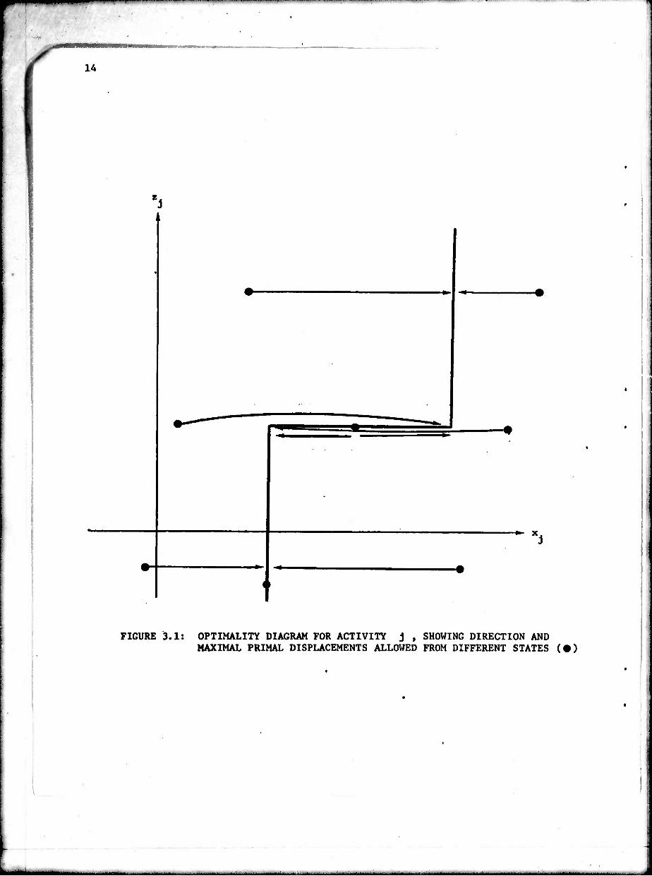
The directions of change and the allowed maximal increments are conveniently

summarized on the Optimality Diagram in Figure 3.1. There are no infinite dis-

placements allowed in the diagram as shown» but if k. - " , or I. ■ -• for some

j , it would be possible to obtain the unbounded solution of (2.8a).

————

1A

t FIGURE 3.1: OPTIHALITY DIAGRAM FOR ACTIVITY J , SHOWING DIRECTION AND

MAXIMAL PRIMAL DISPLACEMENTS ALLOWED FROM DIFFERENT STATES (•)

Mite

•

15

4. BREAKPOINT STEPPING WITH THE INCREMENTAL LINEAR PROGRAM

From the above discussion, the new activity levels x. ■ x. + 5j obtained

by adding the optimal Incremental values from the subroutine to the old activity

levels obviously keep all conforming activities so, and do not move nonconforming

points farther away from or through the optlmallty diagram (see Section 7 for a

discussion of conformity measures). Furthermore, the primal displacement only

permits the following limiting changes of state from iteration t to t + 1 :

r

(A.l)

(a) L" -* L

(b) B" -»- B

(c) K" -^ K

(d) L -•' L

(e) B+ H- B

(f) K+ -^ K

f J ^ Ü lat iteration e)

or

(h) (xj > ij '(■

t+1 j t+1

.)

s) j c B

at Iteration J At least one such change will occur, possibly at a zero-change level.

Hopefully, the selected activity s might undergo a change of type (a) - (f),

but in general, £ may only move partway toward a conforming state, as shown by

the horizontal line in Figure 4.2. In fact, from (2.8d) It is possible that C " <

After these horizontal (primal) movements are made on the various diagrams,

the dual aolution to the incremental linear program fumiehee the appropriate

gradient for vertical (dual) ohangee through the formulae:

(4.2)

(4.3)

t+1

t+1 t *

(1 - 1,2 m)

(J ■ 1»2, ..., n)

and appropriate selection of the gradient etcp size, 6 .

-

mmm —m m

16

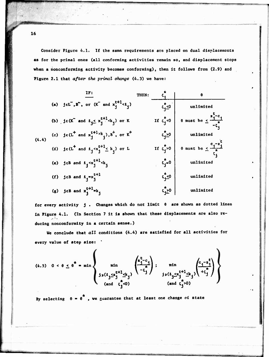
Consider Figure A.l. If the same requirements are placed on dual displacements

as for the primal ones (all conforming activities remain so, and displacement stops

when a nonconformlng activity becomes conforming), then it follows from (2.9) and

Figure 2.1 that after the primal change (4.3) we have:

IF: THEN:

t+1 ü

(A. A)

(a) JeL ,B , or (K and xj ^J

(b) Jc(K and t._< x^ <k ) or K

(c) Je(L+ and xj"*"1^) .B+. or K+

+ t-t-i (d) jc(L and l.<Xj .< k ) or L

(e) jeB and lj<x5+1<kj

(f) jeB and l1-x^+1

(g) jeB and xj"*"1-^

*

V-0

if ct<o

if ^>o

*

<>

te

e

unlimited

6 must be

unlimited

— *

c -z 6 must be < •'■ ■'

J unlimited

unlimited

unlimited

for every activity j . Changes which do not limit 9 are shown as dotted lines

in Figure 4.1. (In Section 7 it is shown that these displacements are also re-

ducing nonconformity in a certain sense.)

We conclude that all conditions (4.4) are satisfied for all activities for

every value of step size: *

(4.5) 0 < 6 £ 0 - min/ min 1*1 ; M M

(and C^O) (and ;.>0)

By selecting 6-6 , we guarantee that at least one change of state

^ _—^ _ 1 " —^^«^-«^^

«*.

17

1

Dual Displace- ments which do not limit 6

-»>Xi

FIGURE 4.1: OPTTMALITY DIAGRAM FOR ACTIVITY j , SHOWING DIRECTION AND MAXIMAL DUAL DISPLACEMENTS ALLOWED FOR DIFFERENT STATES (•)

mmmm

"■I ' —rw^

18

(A.6) (a) K •> B

(b) K~ -»■ B

(c) L H- B

(d) L+ -► B

occurs. If s becomes conforming, then all the ^ may be zero, in which case

* 0 can be set to zero. If the states referred to in (4.5) are nonexistent, and

* 8 is nonconforming, then 9=0°, and the dual solution is unbounded.

Of particular interest is the trajectory traced out by (x .z ) as it is s 8

"worked upon" by the Incremental linear proRram. Suppose first that (x0,z0) e U~ , a s s

an shown in Figure A.2; then the subroutine will maximize C . The result of 8

* * this subroutine will be A = C » creating a nonnegative displacement towards the

right to (x ,z ) , possibly all the way to state K , (or unbounded if »c « •») . 8 8 8

(For z < c , the first step might, of course, be stopped by entry into state L .) s s

* * Then calculation of the dual changes will change z by the amount 6 C

8 8

But, from (2.9) and (3.2), if the horizontal segment does not reach to state K

* * or L , then £ < K , and C B -1 • In other words, the dual change moves the

8 8 S

trajectory'dounuarde by a positive amount 6 to the point (x ,z ) . If 6 *•<*>• t S 6

then the trajectory moves downwards off the diagram, showing dual unboundedness

(I.e., primal infeasibllity—there no basis change at any price which will bring

x up to t ) . B B

The net result Is that, after successive applications of the subroutine, the

trajectory of (x ,z ) describes what Dennis [8] calls the breakpoint curve, a B B

sequence of nonnegative horizontal segments and positive vertical segments which

leads either to unboundedness or infeasibllity, or to an intersection with one of

the conforming "U" states. Similar remarks, "In reverse", apply to the trajectory

traced out by some activity in U , for which the subroutine would minimize £

(See also Section 8 for further possibilities.)

Unselected non-conforming activities also follow a breakpoint curve at each

application of (2.2) and (A.2) upLll conforming, or selected.

^^^i

19 I

.

A* —>

(maximize)

6*

— -z

4. -f i

k .. ,

G nbounded primal

possible only k - «

•—e

(minimize)

:;)

■*• x.

(unbounded dual)

FIGURE A.2: BREAKPOINT STEPPING THE SELECTED ACTIVITY AS A RESULT OF THE INCREMENTAL LINEAR PROGRAM

"^ MM«^..

— -—-—

20

5. GENERAL OUTLINE OF THE ALGORITHM

The «eneral outline of the algorithm should now be apparent. Starting with

an arbitrary solution to the primal and dual, the states of each activity are

identified, using (1.3) and Figure 1.1. An arbitrary nonconforming activity, s ,

is selected and worked upon, using the incremental subroutine. By following the

breakpoint curve. Figure (4.2) either unboundedness or infeasibility is shown, or

s is put in-kilter. Then another nonconforming activity is selected, and so on,

until all activities are in U , and an optimal solution is obtained.

There are still several points to be cleared up, such as the finiteness of

the procedure, both with the regard to the subroutine, and the main algorithm

(Section 7). In addition, there are various options available at each iteration

which can be used in devising various heuristic procedures; these will be

discussed in Section 8 and when comparing the algorithm with others in Appendix D.

We now present the main algorithm.

K*

21

6. COMPLEX; A COMPLEMENTARY SLACKNESS. OUT-OF-KILTER ALGORITHM FOR LINEAR

PROGRAMMING

0. Select arbitrary values of x ■ x. (j ■ 1,2, ..., n)

satisfying (1.1) and y. B y. (i = 1,2, ..., in) . Select an

arbitrary set of m Independent columns for the Initial set

«9- J>0 (Appendix B). Set t - 0 .

1. Identify current states (x ;z ) of activities as J J

U"- L" , B" , or K" ; U - L , B , or K ; U+ - L+ , B+ , or K+

If all J c U , the current solution is optimal.

2. Otherwise, select an arbitrary nonconforming state s .

Solve the Incremental Linear Program

n i

(6.1)

Maximize A - £ c*^* j-1 3 3

(1 - 1,2 n)

(J - 1.2 n)

Minimize k (V:J " W m

u j > 0 , ttj > 0

n. unrestricted

with Initial basis Jt ; starting solution £.

(J-1 n) ;

22

(6.2)

/ 0 J T« 8

1+1 J - s e U~

\^-l j - s e U+

and {X ,K } defined by (3.2).

3. If A ■ +00 , the primal problem (0.1) la unbounded.

4. Otherwise, set

(6.3) xj+1 - *j + ?* (J - 1 n)

5. Find the step size, 6 , from (A.5) and the related

discussion.

6. If 6 - « , the primal problem (0.1) is infeasible.

7. Otherwise, set

(6.A) yj+1 - yj + e*nj , (i - 1,2, ..., m)

(6.5) ej+1 - «J + 6*^ . (J - 1,2 n)

(retain the current optimal basis 4 as the starting basis J

for the next iteration) and repeat Step 1.

, ' ' ' ■ II II

23

7. CONVERGENCK AND FINITENESS

Assume temporarily that the current solution is "primal-feasible", i.e.,

£. £ x. £ k. . By direct substitution, the difference between the primal and

dual functlonals is:

(7.1) ^-C-0- I u.(k. - x.) + I w.(x. - £.) j«! J J i J-l J d J

which will be called the total deviation of the current solution.

In terms of the optimality diagrams, the total deviation is just the Bum of

the individual activity deviations, which are the shaded areas shown in Figure 7.I.

Furthermore, this result does not require k. or I. to be finite, provided

one uses the usual "transfinite algebra" in which the infinite bound is replaced

by a number +M which will be considered larger than any number to which it is

compared during the calculations. Thus to a point like 0 In Figure 7.1, an

area u (M - x ) would be contributed to the total deviation 2> . This is Just

the pricing-in term which would be added to force the point out of the "dual-

infeasible" region above the line z, - c.

A similar device can be used to make arbitrary points "primal-feasible" as

well. For example, if the current x. > k, or < 4. , we may consider that x.

is really an unbounded activity with piecewise linear cost structure

(7.2) cost of activity J ■

VJ +M(W --<*J < ^ VXJ »j IXj^kj

Vkd +M(xj "V "j <XJ-- •

which gives the transfinite extensions to the optimality curves shown in Figure

7.2 (see also Chapter VI, fVj).

"Ufcb «Al MfMHHHI 1 H

■

•

k ..

-,—-»- .IP.... ^i

i

'1 +

FIGURE 7.1: CONTRIBUTION TO THE TOTAL DEVIATION

Z> - C- b FROM "PRIMAL-FEASIBLE" i*yz^

25 r

■ +M

finite portion

transflnlte portion

■•► x.

FIGURE 7.2: CONTRIBUTION TO THE TOTAL DEVIATION -Z?- <J- Ö FROM "PRIMAL-INFEASIBLE" (XJ;ZJ)

■— ——

Direct calculation of^aC-u for the extended problem (7.2) leads again

to the conclusion that the area between the point (x.;z.) and the corresponding

diagram is the deviation due to activity J ; as shown in Figure 7.2, this

deviation may be transfinite only l®| , or may have both finite and transfinite

regions |(g)| .

Thus, as a given activity follows its breakpoint curve, as shown in Figure 7.3,

it follows from the algorithm that:

Every nonzero horizontal or vertical dieplaoement permitted

by the algorithm gives a finite decrease to the total deviation

i7.3)£) = C-B» equal to the decrease in shaded area between the

points (x ;2 ) and the optimality curves, summed over all

activities.

In classical terminology, the displacement from I to II in Figure 7.3

makes activity J "primal-feasible", and from II to III, "optimal" (if k was J

-H» , all vertical displacements reduced "dual-infeasibllity", as well); however,

in our extended definitions, all horizontal displacements decrease C , and all

vertical displacements Increase Ö .

Since the only displacements allowed decrease SO , and since each non-

conforming activity is in the subroutine until it becomes conforming, it is clear

that the algorithm converges.

The only possible source of degeneracy occurs in the incremental subroutine,

where cycling can be avoided by the usual perturbation or lexicographic techniques [A],

Even if the maximal value of A is zero. (2.8), the decrease in SO will be positive,

and a new basis will be selected. Thus the algorithm is finite.

An alternate "finite" proof that an infinite number of steps with 0 finite

■Hi

27

1%0>' Increase In /3

Decrease m <•

FIGURE 7.3: DECREASE IN THE TOTAL DEVIATION JZ>m Q - 0 AS ACTIVITY j BECOMES CONFORMING

28

and with A" » 0 cannot occur is as follows:

(7.A)

(a) Since

(i)

(ii)

(iii)

(iv)

(v)

A ■ 0 , no changes of the type

K K

K

L" -*• L

L+ -> L

(j c B) (x. V (XJ > V (vi) (j t B)

can occur.

(XJ * V (x. V

(b) If an activity moves from L -> B or K -* B during one dual change, its index will enter the basic sgt <0 of the subroutine and remain there as long as A - 0 .

(c) Otherwise, 6 is determined by a transition L -* B or K" -* B decreasing the number of activities which enter Into (A.5).

(d) Since there are a finite number of activities, there can be gnly a finite number of dual changes until either some A is finite ("breakthrough"), or the set in (4.5) is empty (unbounded dual).

'

>

^— ' ■■'— 111 ' >

29

8. ALTERNATIVES FOR THE INCREMENTAL PROGRAM SUBROUTINE

The Incremental linear program (2.2) can, of course, be solved by any method

available; a fairly compact tableau method which utilizes its homogeneous, double-

bounded structure Is given in Appendix A. In this section, we Indicate several

alternative approaches which may be used.

A. Working on Several Nonconforming Activities at the Same Time

If, in fact, a general simplex tableau procedure, as outlined in Appendix A,

is being used to solve the incremental program, then one may wish to do more than

maximize (or minimize) the selected nonconforming activity. In particular, one

may work on all such activities at once, by setting

j c if

(8.1) -c. * i-1 if J e U1"

Instead of (A.l) and (6.2). This does not complicate the subroutine outlined In

Appendix A and may make several activities conforming in one application (with

possibly more pivot steps) of the subroutine.

Or, one may select some of the nonconforming activities to work on—for example,

the activities with transfinite deviations may be worked on first, ss in the usual

"Phase I" ptocedures (Appendix D).

Finally, the magnitude of the coefficients e. is immaterial to convergence

of the algorithm, and one may choose to put more or less pressure on certain non-

conforming activities, based on some heuristic choice; this is the basis for most

proposals which combine "Phase I" and "Phase 11".

B. Primal-Freezing Nonconforming Activities for Single-Step Subroutines

A possibility in the other direction i\ to make the incremental program as

11 "—

30

simple as possible. One way to do this is to "freeze" all nonconforming variables,

other than the one selected, at their current values by setting

(8.2) Xj - ^ - 0 j ^ U + {s}

instead of following (3.2). X or K are set as usual. S 8

In this way, as the subroutine (Appendix A) attempts to increase (or decrease)

£ , only two bounded possibilities occur: 6

(8.3) or

(a) £ reaches one of its own nonzero bounds; the

subroutine terminates with s conforming and the

current basis J) unchanged (but with possibly

* different Cj » J e i) * all c. + c, are un-

changed (equal to e.) .

(b) One (or more) basic £. reaches a bound; s

replaces 1 in the basis by making a pivot on

some a. (A.6). The eubroutine teminatee after Is

one pivot with C, + c. (<1 0 , and all other

0 . J E Jl + {s) . cj + ej

(The usual remarks about ties apply.)

In this simpler, but more restricted procedure, it is clear that no con-

trol is maintained over the sign of ;. , J ^ U + {s} . Thus, other nonconforming

activities may become more BO (i.e., their deviations may increase) at the dual-

changing step which follows. This gives some theoretical problems in convergence,

but in most cases, one can show that one of the functionals is moving in the

correct direction.

mmmmmmm^mi

31

If the resulting value of £ from (8.3) were then such that x were B 8

"primal-feasible", then it would be desirable to choose 6 without regard to the

other nonconforming activities. This would then make s conforming in a eingle

pass through the algorithm, although other activities might "overshoot"—i.e.,

conforming ones might become nonconforming (see D below).

The above procedure is used in the primal simplex algorithm. If several

variables «re brought in at once, the procedure is called "block-pivoting".

C. Dual-Freezing Certain Nonconforming Activities

In a similar way, one can dual-freeze up to m nonconforming variables C. •I

by requiring that their indices be in any basis J of the incremental subroutine.

This restriction then means that the bounds X and K (3.2) for these

variables cannot be effective, and the corresponding (. may have arbitrary sign;

thus these other nonconforming variables may have increasing deviations.

If an attempt is made to make activity s conforming in one step, this may

drive some x. , J c B nonconforming. Thus, this possibility is usually followed

in reverse', i.e., some £ , J e B (c. ■ 0) is moved towards its bound until some

positively or negatively priced C reaches the appropriate bound. This "row-

pivoting" is the procedure used in the dual simplex algorithm (Appendix D).

P. Overshooting Conforming Limit-g

In general, the limits on the £ and et t J 4 U , have been chosen so

that:

(a) no conforming activity passes through a conforming state and then becomes nonconforming again;

(b) no previously conforming activity becomes nonconforming.

As we have seen above, however, when working on a particular activity, or

set of activities, it may be desirable to get this activity conforming "at all

- ■■

-w^- — '"■ ■ ■»

32

costs". This may conceptually be very bad If violating (3.2) or (4.5) makes more

activities nonconforming. However, in certain special cases, we may be able to

argue convergence on one of the functionals.

E. Special Structure Models

Actually, the incremental subroutine, as we see it, is a method for choosing

the direction of the vector {5.} which will maximize the rate of increase of A ,

subject to •][ a^jCa ■ 0 , with certain directions "frozen"; the actual maximum dis-

placement in either primal or dual is of secondary importance.

In problems of special structure, it may be possible to follow through the

effect of changing one variable on the other variables explicitly; then the various

operations of "pivoting" can be carried out in sequential form, without continual

reduction of the matrix to get the current trade-off coefficients ct.. .

The most common example of this kind occurs in network flow models, where the

allowed changes in the {^.} correspond to an incremental increase in arc flows

around a loop including arc s . (Section 10.)

F. Dual-Stepping

Nothing In the algorithm should be construed so as to give a special place to

the primal problem. One can Just as well define the {n.} as the absolute dis-

placements of the {y4) * and work on a selected n through a homogeneous dual

in the incremental subroutine. For example, the pivoting procedure may be clearer

in the transposed matrix (***) •

In this case, nonnegative vertical steps in Figure A.2 are taken first,

followed by positive horizontal displacements, since all degeneracy (at the corner

points of Figure 1.1) arise in the subroutine. Thus, "row pivots" become the

natural changes, and "column pivots" would require looking ahead to the "primal-"

changing step (6.A) and (6.5).

1

33

G. Bound-Tightening

When a given activity is made more conforming, it is possible some other

nonconforming variable may move coherently. If the incremental subroutine makes

several basis changes, it may be worthwhile to "tighten" the bounds on these other

variables as the pivoting progresses to prevent them from "slipping back".

Actually, except for didactic examples, this possibility is quite rare.

H. STARTING SOLUTIONS

In many problems, special starting solutions, basic or not, may be available.

If these are felt to be "reasonable", or near optimal, they certainly should be

used in place of a completely arbitrary solution. On the other hand. If one had

previously found a basic set <0 , and the related Inverse basis in (a..) , then

one should use the corresponding basic solution, feasible or not, solely In the

Interest of efficiency.

I. ARGUMENTS FOR EFFICIENCY

It should be clear from the discussion of this Section and Appendix D that

any prior arguments for efficiency of a certain heuristic, particularly those

based on whether one is moving "inside", "outside" or "on" a certain convex poly-

tope, are doomed to failure.

The COMPLEX algorithm takes any starting solution, basic or not, feasible or

not, and converts it into an extreme point by adding artificial bounds (2.A).

Thus all starting solutions "look alike", in a certain sense, and progress In the

same manner as a basic feasible solution would move over the original polytope.

One would have to make extensive numerical trials for special classes of problems

in order to clearly demonstrate the superiority of one heuristic over another.

Most such experiments have concentrated on how to select a u ^conforming activity

when using the heuristic described In Section 8B above, and starting with laslc

feasible solutions.

■ — '- — 11

s* 34

I

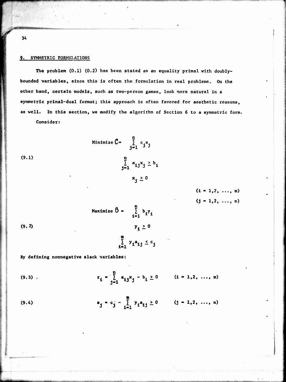
9. SYMMETRIC FORMULATIONS

The problem (0.1) (0.2) has been stated as an equality primal with doubly-

bounded variables, since this Is often the formulation In real problems. On the

other hand, certain models, such as two-person games, look more natural in a

symmetric primal-dual format; this approach Is often favored for aesthetic reasons,

as well. In this section, we modify the algorithm of Section 6 to a symmetric form.

Consider:

(9.1)

(9.2)

Minimize C= \ C4X4 j-1 3 J

X *^ -bi

xj >0

Maximize Ö - \ by 1-1 1 1

Yi 1°

By defining nonnegative slack variables:

(1 " 1,2, •«., m)

(j - 1.2 n)

(9.3) "i " Ji ^J^ ' ^ 1 (1 - 1,2 m)

(9.A) "J " CJ " Ji ^^J '

(j - 1,2 n)

—+

——

n 35

the constraints in (9.1) and (9.2) are changed to equalities; since they will

remain equalities during the algorithm, they are henceforth ignored, and all

attention is focussed on the extended variables:

(9.5)

k-n

(k - 1,2 n)

(k «= n+1, n+2 n-hn)

(9.6)

h rk-n

(k = 1,2 n)

(k ■ n+1, n+2, ..., n+m)

where k runs over the range (1,2, ..., n;n+l, n+2, ..., n+m) to take In the

appropriate real or slack variables. The extended constraint matrix of (9.1)

consists of CaJj) augmented by an m x m negative identity matrix:

(9.7) (o^) - (Ca^), -I)

The restatement of the Optlmality Principle (1.5) is:

Optimality Principle

A feasible solution of nonnegative values Y^.i it.} i vs

optimal if and only if (9.8)

V ft -0

for all k - 1,2 mfn .

The optlmality diagrams corresponding to (9.7) are shown in Figure 9.1. Note

that this figure is reversed and normalized from Figure 1.1. Thus, the breakpoint

trajectories will have reversed "dual" changes. Increasing (decreasing) from left

to right (right to left), tfc keep the same states L , L , L , B~ , B , and

K~ as before ior the current extended state S^yX jfi\ •

p»!! ■■ I , »»■■ ! ■ ^ —I- m,

36

FIGURE 9.1: OPTIMALITY DIAGRAM FOR SYMMETRIC FORM

37

For completeness, we restate the algorithttuof Section 6 In symmetric form;

some details on the extended tableau are given In Appendix C. No proofs of the

algorithm need be given, since the extended problem Is exactly In the form (0.1)

and (0.2). However, some "complementary pivot" Interpretations are given In sub-

section B.

A. Symmetric Form of the Complex Algorithm

0. Select arbitrary values of x. ■ x. (J ■ 1,2, ..., n) and

y - y° (1 - 1,2, ..., m) and use (9.3)(9.4) to calculate

the remaining components of </»..> and <(ri.> •

Select an arbitrary set of m Independent columns Ji , In

the extended constraint matrix, (AJJ) (say, the negative

identity matrix of the last m columns).

Set t - 0 .

1. Identify the current states ML: ^k) of all variables as

U" - L~ , B" , or K" ; U - L or B ; U+ - L+ . If all

k e U , the current solution is optimal.

2. Otherwise, solve the Incremental Linear Program:

tttn Maximise A - I ev^ir

k-1 * *

(9.9) J/iA"0

(1 - 1,2 m)

(K m 1,2, •••, m+n)

,

-■-

38

(9.10)

in+n Minimize I ^W - \\>

k-1

1 ^ ^ailc - Uk + \ "

^ 10 ; «^10

n. unrestricted

-E.

(i - 1,2, ..., m)

(k " 1,2, •••, m+n)

with initial basis Jt , and starting solution Ck - 0

(k ■ 1,2, •••, m+n) •

The coefficients in the functional have arbitrary value

and sign:

I

(9.11)

k e U

elt < 1 0 k c U

< 0 k c UH

selected to work on one or several nonconforming variables at

the same time

The bounds are:

(9.12)

k Xk \

L' 0 K B" 0 -

K" 0 a»

L 0 0

B »i -

L+

< 0

3. If A • -H> , the primal problem (9.1) is unbounded.

4. Otherwise, set:

■^

!^ ' '• "■ ■" m"-

f

39

(9.13) ^r1 - %l + C (k - 1.2 m+n) kk

* 5. Find the step size 6 from

(9.1A) 6* - mln k Wl <**)

(9.15)

where only Indices k are allowed for which: Jjf. >_ 0 ;

the denominator is nonzero; and the numerator and

denominator are of the same sign.

6. If the set of indices in (9.14) is empty, G - " , and

the primal problem (9.1) is infeasible.

7. Otherwise, set:

iit+1 tit * r * !rk -^k-6 ^Vik (k-i.2 »+«)

and repeat Step 1.

B. Complementary Pivot Methods

Appendix C points out how certain of the basis changes in the extended

matrix O^J) can be Interpreted as "dual pivots", in the sense of the row operations

of the dual simplex method (Appendix D.A). This symmetrization is formalized In the

complementary pivot methods of Cottle [3], Dantzig [6], and Lemke [12], which were

developed for a larger class of problems (Section 13).

Instead of the extended variables (9.5)(9.6), attention is focussed on the

variables:

(9.16)

(9. 17)

,.(% (k - 1,2, ..., n)

k ^k-n (k ■ n+1, n+2, ..., n+m)

k lrk-ii

(k - 1,2, .... n)

(k - n+1, n+2, ..., n+m)

" '

AO

This has the effect of reversing the axes on the last m optimallty diagrams of

Figure 9.1, thus making the "real" dual variables y abscissae, together with i

the "real" primal variables x . The problem (9.1) (9.2) is also usually stated

as a combined (mfn) x (mfn) primal-dual problem, together with feasibility

requirements which are identical with the optimality requirements (9.8).

In terms of our model, complementary pivot theory stresses the case when

exactly one pair of complementary variables, say (zh;Mi ) in (9.16) (9.17) is

nonconforming; this Implies exactly one other pair is at the LB comer point, say

2 ■ W " 0 (possibly more than one if there is degeneracy). This point e is

then moved into either L or B in a manner to reduce the nonconformity of the

variable h , some other variable £ then moving into its corner. If i moves

into the corner on B , it leaves on L at the next iteration, and vice versa;

this is what is meant by complementary pivoting, and is a natural observation from

the incremental subroutine of Appendix C. The procedure, of course, terminates,

when variable h becomes conforming.

Actually, starting with Just one nonconforming solution pair (2.; W^) is

quite difficult, in general, and the only starting solution methods proposed [5]

seem to require Introduction of artificial variables. Following the effect of this

proposal through in terms of Figure 9.1 reveals:

(a) All initial and subsequent solutions are in L , B , or B ,

or

(b) The nonconforming point(s) which is(are) currently farthest

away (in a linear sense) are worked upon.

(c) Primal- and dual-freezing are used as needed to keep all

solutions in the above states.

These special rules then reduce the complementary pivot procedure to a combination

of the primal-simplex and dual-simplex procedures, that is, a .:->•. >oslte method

(Appendix D. I;-

(/k <0 ",d afk -0) •

■-.— 1—-— ""•

41

However, we have previously seen (2.7) that the. incremental program, (2.2)

or (9.9), is already In complementary pivot form, since only C " 0 Is noncon- s

forming at the beginning of the incremental subroutine. Thus, the COMPLEX approach

essentially reduces every initial solution to a related complementary pivot problem.

In addition, the nuisance problems of infeasibility and unboundedness are handled

separately.

C. A Doubly Double-Bounded Symmetric Problem

As an ultimate symmetric variant, the reader may wish to try rewriting the

algorithm of subsection A for the following doubly double-hounded Symmetrie problem:

n m Mint" \ c,x - \ [d.max(0,r ) - e.max(0,-r,) ]

J«l J J 1-1 1 1 1 1

(9.18)

}ml aiJXJ " 'l - bl

(1 - 1,2, ..., m)

(j - 1.2 n) m n

Max :Z> - J Ny< + I [l4m«x(0t8.) - k.iii«x(0,-84)l 1«1 x x j«i J J J J

(9.19)

whose optimality diagrams are given In Figure 9.2 a and b.

A2

D. Genoral Piecewlsc-Linear Convex Costs

It is also appropriate to remark that the COMPLEX algorithm can easily be

extended to general pleccwise-llnear convex costs. The resulting optlmallty dia-

grams would then have many horizontal and vortical segments; only a few details

In the algorithm would need to be changed. (Sec also Section 12 and [8].)

■ /

'

: -.—■^. - ,-» ^ ■ - ■

1"

•H

43

i

i

f

£

€<*

-1t*almmallmtumm

——- ■■ ' —'■■ " ■■ii I I I I IIWI, IIIB r-

"

^4

10. NETWORK FLOW MODELS

A special class of problems of great practical Interest are the network

flow models [9,10,14] for which the constraint matrix Is the node-arc Incidence

matrix, giving either Klrchoff's Current or Voltage Laws In the primal or dual.

For these models, the homogeneous Incremental program takes on the following

simple form:

(a^ Find a loop (cycle) of special arcs in the network that can take an Incremental amount of flow;

(10.1) or

(b) Establish a set of potentials on each node, so that the sum of potential differences around any loop of special arcs Is zero.

Either or both of these steps Is handled In netowrk problems by means of a simple

labeling technique, which Is merely a way of "unraveling" ' Jfects of i pivot

change; by changing the flow variables around a loop (adding an Incremental

oiroulation flow), one. Increases or decreases only the variables necessai,. to keep

the flow conservation laws satisfied. (If the problem is stated In single source-

sink form, the pivoting procedure may find a flov-augmenting patl .) As usual,

determining the actual bound on the Increment of flow, or determining the changes

in potential to "break down" a new loop, are secondary calculations which can be

performed independently. Thus, the calculations proceed from a basic solution (a

tree of arcs), adding a new vector (a octree arc which forms a unique loop with the

tree), through a pivot change (determining an arc in the loop to be removed), to

the new basis (another tree).

Viewed in terms of the optimality diagram and the algorithm of Section 6, the

various methods can be viewed as follows:

(a) The stepping-stone methods are primal simplex algorithms which always maintain baf/». primal-feasible solutions as shown in Figure D.I. A set oZ potentialSj placed on the basic tree, -'ekes a cotree arc nonconformlng. Then, flow is rerouted to deLeii.-.tne a new basic solution, and so on until optimal.

'f 45

(b) The Hungarian-Ford-Fulkerson methods were responsible for the development of the general primal-dual method for linear programs discussed in Appendix D and F. Usually all non- conformity is placed on the return arc from sink to source, which starts with zero flow. Thus, incrementally least-cost flow-augmenting paths are sought until all flow is allocated.

(c) The out-of-kilter method is exactly the algorithm of Section 6.

Actually, after the important early papers of Ford and Fulkerson see [9,14] for

references) the state-of-the-art was such that many people realized that the

complementary slackness conditions were the key to dealing with arbitrary initial

condition (Appendix A of [10]). In fact, an independent development of the out-of-

kilter approach may be found in the 1958 thesis of J. B. Dennis [8]. The emphasis

Is on electrical analogues, and elementary activities (Section 12), but his

"black-box" approach, and "breakpoint-tracing" are identical to our notion of a

selected activity, and sequential primal-dual changes needed to force this activity

to bo conforming. This Important paper treats general programming problems in

this same light (Sections 12 and 13).

One can also extend the simplified pivoting of ordinary network flows to

problems where there are arbitrary multipliere of flow on each «re [10a], giving

«rbitraiy coefficients in the node-arc incidence matrix. However, here the

appropriate basis is not a tree, and the appropriate "unwound" form of a pivot

step is to find a flow-abeorhing loop in the network. Extensions to multi-com-

commodity flows have also been suggested (see, for example, [10b]), but here the

efficiency of the algorithms is less satisfactory.

- ■ - ■ ■ ' - ■ ■ - -

A6

11. THE SIMPLEX METHOD AND ITS HEURISTICS

By this point, our central thesis should be evident:

all the extreme point methods of linear pvogramrning are

equivalent to the original simplex method,

modified by the following heuristic choices:

(a) How Is the problem formulated—inequalities, equalities, symmetric form, self-dual, upper or lower bounds, etc.?

(b) What initial solution. If any, is available for the primal and/or dual?

(c) Is the Initial solution basic, or Is a natural starting basis available?

(d) Which group of nonconforming variables Is to be worked on first? Is any subset to be worked on simultaneously, or will they be handled Individually? What criterion of nonconformity selects among these?

(e) What Is the attitude towards the other nonconforming variables? Are they to be bounded towards conformity? Primal- or dual-frozen? Ignored?

(f) Is a general simplex (pivot) subroutine to be used, or a special al- gorithm? Will it do primal steps first, or dual steps?

(g) Are single-pivot changes to conforming states to be made? How much primal- or dual-change overshooting Is to be allowed?

The primary advantage of the algorithm presented here is a pedagogical one,

that different variants are easily presented, and compared. Also, the problem

does not need to be forced Into any artificial format; construction of the ap-

propriate optimallty diagram always "reminds" one of the appropriate procedure

to be followed.

Finally, the COMPLEX algorithm presents a general framework within which new

heuristics can be explored; certainly the basic similarity of the various break-

point curves suggests that questions of relative efficiency must be decided com-

putationally, and not on the basis of whether a solution stays feasible in a

certain sense, or always mrVes some activity conforming at each step. In this way,

we distinguist- between the theory and the art of optimization.

, __. ^^-__.

..**

47

12. BREAKPOINT-TRACING ELEMENTARY ACTIVITIES AS BUILDING BLOCKS AND THE

BREAKPOINT-THEORY ALGORITHMS OF J. B. DENNIS

In this section we will consider the "construction" of an arbitrary linear

program ftom certain elementary activities. In this way, we hope to shed some

light on the pioneering work of J. B. Dennis [8].

As one analyzes the mechanism of the simplex algorithms. It becomes clear

that there are only a certain number of elementary operations performed, and

that each regular activity could be thought of as a composite of simpler

elements. Typically, we have: a "pricing" mechanism which turns an activity

"on" or "off"; a primal (In)equallty; and a dual (in)equality.

The three canonical elementary activities might be:

(s) (a) a no-cost switching variable x^ , which turns other

activities "off" and "on" to arbitrary levels, whenever

the pricing Is negative, or tries to go positive.

(Figure 12.1 a)

(12.1)

«j00 > 0 ; c<8) - 0

.(c) (b) an unbounded oonatant-ooet rate activity *\ • vhlch

"costs" or "profits", as the activity level Is

positive or negative. (Figure 12.1 b)

^ x. i » c. (O .(c) 'J • 'J

.00 (c) a aonatant-level activity, x* , independent of

pricing and costs. (Figure 12.1 c)

xjk) - k ; (c.00 - 0). zj(k) unrestricted.

A8

MM

N a

I

0)

N

PQ M W

8

CM

0) S fc

- ■ ^ ■ - _^_J^__

■'

A9

To build up composite activities, we use the following construction rules

between two arbitrary elements with given optimality diagrams, (x^jz.) and

(x2;z2) , to construct a new activity (x0»0 •

(a) "Series" Combination

Xo " xl " x2 J Zo = Zl + Z2

(b) "Parallel" Combination

(12.2) xo - x1 + x2 ; 2o - z1 - z2

plus the unary operation:

(c) Traneformation

x - Kx. ; z ■ Kz. o 1 * o 1

In this way, compound activities with very general 'btaircase" diagrams can be built

up. For example, the compound activity shown in Figure 12.2 (a) can be built up out

of the five elementary activities shown in Figures 12.2 (b) - (f) by adding the

three constraints

+ x2 + x5

(12.3) 0 - - x2 + x3

0 - -Xj " x3 + x4

and substituting x in whatever other constraints hold for the compound activity.

Rearrangements of (12.3) suggest the various ways in which the "assembly" of

(x • z ) can occur, o» o

L

mr^mmrm

c*t

r-4

Ä. in

N -

CO

en

§

O

I o

M H O

| H

O CJ

N

g

K

.«n

.

•

CM

.

o

r H O

w

s s CO

CM

I u M

51

Such an expanded representation naturally leads to many more elementary

activities than real ones. But, conversely, the various simplex operations

degenerate considerably for the types (12.1), and it may be possible to devise

special algorithms for hand calculations, particularly when the problem is

"weakly connected".

The use of elementary activities is nothing more than a faithful transcription

of the -idedlized current elements (diode, voltage source, current source) in

J. B. Dennis* 1958 thesis [8]. The notion of breakpoint stepping and operating

with the optiroality diagrams are also his; and, from a certain viewpoint, this

entire paper might be said to be a natural interpretation of his method.

But, for some reason which this author does not understand, very little

attention has been paid to this fundamental paper; in the next section we shall

see that Dennis* breakpoint-stepping ideas can also be used in a larger context.

-- - i

■' ■ -—'"■", - . ..

s

WM

-

52

13. EXTENSIONS

Wolfe [16] has shown how quadratic programs can be calculated by applying

complementary slackness conditions to an enlarged problem In which the primal and

dual variables are "coupled" by linear relationships. The basic outline of an out-

of-kilter method for these problems was given by Dennis [8], who Introduced the

idealized elementary activity which has a straight line U, ■ R. 3». optimallty

diagram (a "resistor"); there appears to be no difficulty in extending this

approach in the directions we have outlined here. Recently, Lemke [12] has shown

that bimatrix games can also be put in complementary pivot form, which would then

represent another extension for arbitrary starting solutions. In both these cases,

the breakpoint curve consists of straight lines at arbitrary angles, as well as

horizontal and vertical segments, and the appropriate theory may be found in [8],

Chapters 5 and 6.

In principle, it would also be possible to extend these ideas to general

convex programming, provided that one knew how to move both primal and dual ,

solutions simultaneously along the monotone optimallty curves defined by the

Legendre transformation which gives the dual problem. For this reason, nonlinear

solution methods appear to depend more strongly on special initial conditions than

linear methods do. Another well-exploited procedure is to use quadratic

programming as a local approximation (Chapter 7 of [8]).

-

f 53

REFERENCES

fl] Ballnski, M. L. f and R. E. Gomory, "A Primal Method for Assignment and Transportation Problem," Management Science. Vol. 10, No. 3, pp. 578-593, (April 1964).

[2] Ballnski, M. L. , and R. E. Gomory, "A Mutual Primal-Dual Simplex Method," Recent Advances In Mathematical Programming. R. L. Graves and P. Wolfe . (eds.), McGraw-Hill, New York, pp. 17-26, (1963).

[3] Cottle, R. W., and G. B. Dantzig, "Complementary Pivot Theory of Mathematical Programming," Technical Report No. 16, Department of Operations Research, Stanford University, (June 1967).

[A] Charnes, A., and W. W. Cooper, MANAGEMENT MODELS AND INDUSTRIAL APPLICATIONS OF LINEAR PROGRAMMING, Volume I. John Wiley & Sons, New York, (1961).

[5] Dantzig, G. B. , LINEAR PROGRAMMING AND EXTENSIONS, Princeton University Press, Princeton, (1963).

[6] Dantzig, G. B., and R. W. Cottle, "Positive (Semi-) Definite Matrices and Mathematical Programming," ORC 63-18, Operations Research Center, University of California, Berkeley, (May 1963).

[7] Dantzig, G. B., L. R. Ford, and D. R. Fulkerson, "A Primal-Dual Algorithm," In H. W. Kuhn and A. W. Tucker (eds.), "Linear Inequalities and Related Systems," Annals of Mathematics Study. No. 3, Princeton , University Press, Princeton, pp. 171-181, (1956).

[8] Dennis, J. B. , MATHEMATICAL PROGRAMMING AND ELECTRICAL NETWORKS, John Wiley & Sons, New York, (1959).

[9] Ford, L. R., Jr., and D. R. Fulkerson, FLOWS IN NETWORKS, Princeton University Press, Princeton, (1962).

[10] Jewell, W. S., "Optimal Flow Through Networks," Interim Technical Report No. 8, (Sc.D. Thesis), Operations Research Center, Massachusetts Institute of Technology, Cambridge, Massachusetts, (June 1958). (Out of print.) The two main algorithms of this report were republished as:

a. "Optimal Flow with Gains," Operations Research. Vol. 10, No. A, pp. A76-A22, (July-August 1962).

b. "A Primal-Dual Multicommodity Flow Algorithm," ORC 66-2A, Operations Research Center, University of California, Berkeley, (Septeirber 1966).

[11] Kelley, J. E., "Parametric Programming and the Primal-Dual Algorithm," Operations Research. Vol. 7, No. 3, pp. 327-33A, (May-June 1959).

[12] Lemke, C. E., "Bi Matrix Equilibrium Points and Mathematical Programming," Management Science. Vol. 11, No. 7, pp. 681-689, (May 1965).

[13] Orchard-Hays, W. , MATRICES, ELIMINATION AND THE SIMPLEX METHOD, C-E-?-R, Inc., Arlington, (1961).

WP—IW^Wi^^——^—W^WI I ■! III I 11 I ■■■! I 1

54

[14] Simonnard, M. , LINEAR PROGRAMMING, Prentice-Hall, New York, (1966).

[15] Wolfe, P., "The Composite Simplex Algorithm." SIAM Review. Vol. 7, No. 1, pp. A2-5A, (January 1965).

tl6] Wolfe, P., "The Simplex Method for Quadratic Programming," Econometrlca. Vol. 27, No. 3, (July 1959).

V* I— ■ " ' ■—

A.l

APPENDIX A. ORGANIZING THE INCREMENTAL PROGRAM TABLEAU

Because the incremental program subroutine (2.2) and (2.3) Is In a special

form, in this section we consider how calculations might be carried out in tableau

format. Naturally, to develop an efficient procedure for computer calculations,

■any other factors, such as size of storage, round-off error, matrix sparseness,

etc. must be considered. As discussed in Section 8E, special algorithms may also

be available for problems with special structure. Howevor, the procedure outlined

below is adequate for hand calculations and as a starting point for planning com-

puter organization.

There are two novel features of the Incremental program:

(a) it is homogeneous;

and (b) its variables are doubly bounded.

The first fact gives an easy starting solution in all cases; there is also no

right-hand side to keep track of. To use (b) efficiently, the upper and lower

bounding relationships are calculated outside the main tableau, and we keep

separate track of the current values of the "nonbaslc" variables which are at

their upper or lower bounds.

A suggested format, as it might appear at the start of the first Iteration is

shown In Figure Al. T*16 coefficients UJJ) are placed in the main m x n array.

In the next row above are placed the "pricing" terms, C. + e. , with

(Al) (+ 1 if c 1 s

is to be maximized

S' (-1 l£ C. is to be minimized

V l^.t

But see Section 8A for other possibilities.

—I

A.2 (0 0) U

S n) 0) M

H -H (0 U 0) H u a w 3 rt O O -H Q > > (0

•H MO«

N

H

iH

H

<N

O

O

o

o

<0

w

I ä§ M «

O H 2 H H » H

CO H

go

S i

§S2

M

Uf

+ OJ

a a iH id «o « g 4J (0 9 C a» o a» H P5 e 43 «MM

U M 01 C «Ö .C M > H

g"

0) «J 0

O -H U

45 U-l u at 55

^

A. 3

Since the current values of the variables arc "lost" during an upper- (and lower-)

bounding technique, the U } are displayed, together with the current values of

the {K } and {X } , in three rows above the pricing terms.

For completeness, an m x m unit matrix is adjoined to the matrix of coeffi-

cients so that the dual variables (n.) and the inverse of the current basic are

obtained automatically. In a computer code, a more efficient scheme such as the

product form of the inverse would be used.

Once the initial basic set of variables, Jl = J , is specified, then the

tableau can be reduced to the normal form shown in Figure A2 by the usual Gauss-

Jordan reduction procedure, and the relative prices {; + e.) reduced to zero for

j e J) . This simultaneously gives the inverse of the current basis and dual

variables for the incremental program. Pivoting operations are carried out in each

application of the subroutine using the rules below; the last form of the tableau

in a given Iteration can be used to begin the next application of the subroutine

(Appendix B). ,

In a doubly-bounded procedure, all basic variables satisfy:

(A2) ^ 1 Cj i Kj ; ^j + ej = 0 J e J •

The nonbasic variables are at their upper or lower bound, and, at optimality (2.9):

If ; + £ > 0 C* - ►:. ; (A3) J 3 I •l j ^J.

if ;; + ej < 0 5j - Xj

\

r A.4

I o

§ M H

H

M

I Si w

ii

u/

+ CM • t «CO • •■ • Ö

I ■

A.5

Thus,

Rule for Selection of a Candidate to Enter the Basis

Scan the Pricing Row for Some Nonhasic Activity eiA such that

(a) C + e > 0 and t, < < e e e e (A4) (b) ; + e < 0 and J; > X . or e e e e

(i) If none exist, the current U.) , (n.) and UJ are optimal

(11) Otherwise, £ Is a candidate to enter the basis.

Now, if some ^ Is to enter the basis from Its lower bound, a positive [negative]

trade-off coefficient, a. , In row 1 , column e of the tableau Indicates that

the basic variable Cj/.\ corresponding to row 1 (i.e., the unit matrix has an

entry In column Ä , row 1 ) must decrease [increase]: the bound ^»/i^l^a/■<\1

may thus limit the Increase of C «as will Its own bound, K . Similar remarks

apply If £ Is to enter the basis from its upper bound.

The smallest such change determines the actual change to be made in C :

If it is a basic variable t./.,\ which reaches a bound, £ replaces *•»(*}

in the basis, with a as pivot; if £ goes all the way to its other bound, X6 "

the basic set of variables remains unchanged, and only the values of the £.

are changed. Obvious remarks apply to ties and unböundedness.

Thus follows: *

Rule for Selection of Candidate to Leave the Basis, and for Changing

the Values of the Incremental Variables

1. For a given candidate activity e , a nonzero trade-off coefficient o. ,

(A5) and the corresponding basic activity A(l) , partition A into the following

sets, and define the indicated displacements, 6. , for all J e J + (e)

A.6

111

(A6)

(a) l(i) e J " iff

r, + t > 0 and ou < 0 c e ie

or ; 6, .C + e < 0 and a. > 0 e e ie

fC + e > 0 and a, > 0] e e ie

(b) Hi) EJ iff (or U + e < 0 and a, < 0^ e e ie

>rV/(-aie^

'(^-\)/(-aie)

(c) Otherwise Ä,(i) e J) - / - J" : ^j^ E *

(d) Define 6 K - £ If c + e > 0 e e e e

1 e e e e

2. Compute the allowed displacement, 6 .

(A7) 6 = min ( 6_; miij 60; min 6 e' HCJT ^ilei" "'

(a) If 6 = o0 , the incremental program is unbounded. (Return to main

program with Ä = ^ .)

(b) If the minimum 6 in (A7) is computed from Jl or Jl , then

activity e enters the basis at level 6 < 6 , driving some basic

activity I to its lower or upper bound, whence it leaves the basis.

Pivot on the appropriate a. and reduce all rows of the tableau plus

the pricing row to normal form with the new basis * - Jl + {e} - {J.}

(c) If 6 is determined by 6 , then C goes to a bound, and the c e i

current basis J remains unchanged. Jl « J) .

(d) In case of a tie, the choice is immaterial (avoid a pivot operation,

if possible).

W»*I"^""T— — "—'

:i 3. Compute the new values of the {£; } :

C. - I. + 6

e 1- 6

(C + t > 0)

^ + 6 If j c /

C - 6 if j e J"

= ^J If j e J- J+ - J'

•

Then, a new candidate is selected, using (AA) , and the steps are repeated

until the optlmallty criterion (A3) is satisfied. Control is then returned to the

main routine, with the optimal values U } , {r^J , and (c.) from the appropriate

* r. * points of the tableau, and A ■ ^ t. C- .

The next call for the subroutine will clear U.}, ..., and give new values to

U.} {ic.} and {E.} ; however, the rest of the tableau can be saved in its last

. * (reduced) form, with the optimal basis J from this iteration (Appendix B).

■.

■ ■

■■ ■'■"

—n ig; j

B.l

APPENDIX B. SELECTING THE INITIAL AND SUBSFQUENT BASIf.

To get the incremental program subroutine started, it is necessary to specify

an initial basic set «5 . However, since C. = 0 for all variables at the

beginning of each of the subroutines, any selection of m-independent columns of

(a ) will work. Typically, some slack, or error variables were added in the

formulation which provide convenient unit vectors. At worst, with a full matrix,

an arbitrary element can be selected to clear its column; any dependent columns

will show up as columns of zeroes and cannot be used. Note that "frozen" variables

0 < C. 1 0 (X - ic - 0)

can conveniently be regarded either as basic variables, or as nonbaslc variables

at either bound.

Once the tableau has been put in normal form, It is probably most efficient

and convenient to leave it In that form, making further changes only by pivot

operations. To do this, the following result Is needed:

The optimal basic sett J) , from one iteration of the program

(Bl) subroutine may be used as the starting basic set J for the

next iteration.

The proof Is trivial, once we note (2.9), the fact that all £. are reset

to zero for the next iteration, and the remark about frozen variables itada above.

Suppose the objective coefficients at Iteration t were e. (J - 1, ..., n);

* the optimal values of the (5 } can be determined directly from the pricing row

ti »t* of the first tableau by subtracting {e.} . Then, If the same basic set, J> ,

is kept to start the (t + I)8 iteration, one changes the nontableau rows

mmmmmm

B.2

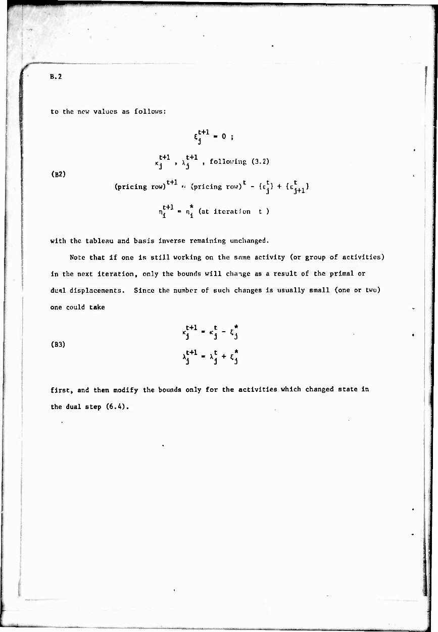
to the new values as follows;

(B2)

^ -0 ;

t+1 t+1 , ,, . /, o\ K , \ , following (3.2)

(pricing row) " (pricing row) - {e.} + {ej+i)

t+1 * n. ■ n. (at iteration t )

with the tableau and basis inverse remaining unchanged.

Note that if one is still working on the same activity (or group of activities)

in the next iteration, only the bounds will change as a result of the primal or

deal displacements. Since the number of such changes is usually small (one or two)

one could take

(B3)

t+1

^t+1 j

t r*

t *

first, and then modify the bounds only for the activities which changed state in

the dual step (6.4).

—

•

•

C.l

APPENDIX C. THE INCREMENTAL PKOf.!:.' ■ i''.l.l .^ } O't TIT SYMMETRIC PROBLEM

In the symmetric problem of Section 9, a negative unit matrix is in the

formulation explicitly; by extending the indc :: of t, from 1 to m + n , we get

the incremental changes on the {r.) as well as the {x } . Figure Cl shows

how the tableau might be organize J; J might as well be taken as the last m

columns. Note that bounds and pricin,' no., apply to all m + n columns; if one

of the last m columns is basic, a slack cliunge may occur. At optimality, the

* + Lk . (1< 1,2. .... n) or -n*_n+ ck , * *

pricing row actually contains r + L. , (1< 1,2. .... n) or ~\_ + E

(k = n+l,n+2. .... n+m) •

If there is a "slack" column in J which prices out incorrectly at some

Iteration, we see that clearing the pricing row to zero in that column will intro-

duce price changes in the first n columns, and thus a nonslack variable will

become a candidate to enter J. This step will in fact be a dual-pivot

as described in the dual simplex algorithm. Appendix D.D. A more compact,

symmetric form could be obtained from a condensed tableau form of Cl with rather

complicated row and column-pivot rules (2]; however, rather than strive for

complete symmetry, we leave the procedure here in its expanded form, so that

the (negative) inverse of the current basis is always available.

■ I

C.2

I o

o

o

J - - - . . ■ | | | | l i M i ■

f-i I

U-l o

in 0) -H in in U (4

> c u u

« 60 0)

<u >

M O

O

o

o

.* u1

■n ■H

&d o £ t>

ss KJ

(0 3 u H c 0) •H ^ u M •H H «M M iM Z 01 M o u <4-< rH o u

•S 1 u 3 u Ü

5 PL,

* * *

g «J m u C^ e oi -H 0» ^ 0) 60 i U3 J3 « c 0* «0 H T3 •H Si TH (i U

U 13 9 Ti Ü « c o u M > (0 ea 04

_u

,.: 1 APPBMDIX I). COMPARISON WITH OTHER SIMPLEX Al.nop.TTHMS

To fully appreciate the relationship between the COMPLEX method and

the many special algorithms which arc in current use, it is instructive to

explain the possible variants in terns of the optimolity diagram.

A. The Primal Simplex Alporith-n

In its primitive form, a problem is formulated using unbounded, nonnegative

variables; nonnegativo "slack" variables arc added at no cost as needed to change

all constraints to equalities. It is assumed that a primal-feasible basis, B

of nonnegative (x } is known; the nonbasic variables have value x. = 0, j ^ B .

Dual variables are determined by solving:

(Dl) V ^ yi a ■ c U J

j e B1"

and thus we may have;

(D2)

< c,

J i Bf

(If z. ■ c. , we may perturb the c. , so that B corresponds only to our

set B ).

On the simplified complementary-slackness diagram (Figure Dl) , all basic

variables © are on B , while nonbasic variables are either conforming in L( CD ),

or nonce iforming Q) (in K )'with x - 0 .

An arbitrary activity, e , of type (3) is selected to enter the basis,

and x B C is maximized while primal-freezing all other nonbasic variables, e e

including the other nonaonforming ones; horizontal movement of £ is unlimited

until some activity t. in B reaches its lower bound zero, and thus leaves

the basis and is considered as an activity of type ® . As discussed in Section 8B,

this means that the incremer^al subroutine consists of a single pivot operation;

the dual changing step öotemines 9 so as to make activity e dual-conforming,

.,.*,

D.2

Decrease in ^

© 4 -- n

©

■* *A

FIGURE Dl: OPTIMALITY DIAGRAM FOR SIMPLEX ALGORITHM SHOWING BASIC AND NONBASIC ACTIVITIES, AND PIVOT STEP

1^"

D.3

since it is "brought into the basis B " (i.e., will be used to calculate the

z from (Dl)). This forced conformity may possibly lead to dual "overshooting,"

some conforming nonbasic activities become nonconforming, and vice versa. (Activity

t , however, will always move into L .)

The single-pivot procedure is repeated with the new (possibly enlarged) set

of nonconforming activities, until all are made conforming, basic or not. At

each step, the decrease in the primal functional C is the shaded area shown,

and convergence (except for degeneracy) argued on this fact.

Sometimes the candidate e is not selected arbitrarily, but Is chosen

from among those which are "highest above B ", or "will give the greatest area"

on their respective diagrams.

B. Artificial Variables

Getting a primal-feasible basis BP can be a nuisance. If a unit matrix

of appropriate sign cannot be found In (a^j) . then nonnegative artificial variables,

x , are placed In BP as needed. Since they must ultimately satisfy x - 0 ,

they are given a transflnlte cost M (Figure D2a) , but are considered conforming.

In this "method of penalties", solution of (Dl) gives transflnlte "nonconformities"

M(z. - c ) to some of the ordinary variables; then application of the primal

simplex algorithm removes these artificial variables, one at a time, to position

(2) In Figure D2a whence they are Ignored. (Assuming primal feasibility). Since

finite z - c discrepancies are Ignored during this procedure, further finite

steps are still needed to correct any activities which are or become finite

nonconforming.

mmt

M

D.A

M L ©

^»

®

-♦ x

(a). Method of Penalties

c = 1 'i

®

©

(b) . Two-Phase Method

■♦ x

i

T z

T

k-i- i

* -

Slack Not Allowed

Slack Allowed

(c). Nonconforming Approach

FIG'J;" D2: OPTIMALITY DIAGRAMS FOR ARTIFICIAL VARIAS L.J

,—^

D.5

In the "two-phase method," transfinlte numbers are avoided, but a separate

cost functional, with:

(1 J artificial (D3) c =

-' ' 0 j ordinary

is used in "Phase 1" (Figure (D2b)). This procedure will (if the problem is

primal-feasible) drive all the x to zero. In "Phase II", these variables

are frozen at zero, and the ordinary functional C is taken up, since a primal"

feasible basis B of ordinary activities is available.

As is well knovn, the above two methods are equivalent.

In the formulation of our algorithm, these variables are treated either as

error variables which are to satisfy x =0 (dotted line in Figure D2c), or aJ

as nonconforming (negative) values of slack variables (solid line in Figure D2c).

In our approach, these would individually (cr jointly) be made conforming, follow-

ing the usual breakpoint procedure. To obtain the same sequence of steps as the

above methods, however, one would need to:

(a) Take all of these artificial variables as (part of) the

initial basic set J ;

(D4) (k) Set t " 1 for these variables in the subroutine (2.1);

and (c) Ignore the nonconformity of the variables not in J) until after

all these special variables have been made conforming (i.e., until

the next application of the subroutine).

C. Combined Methods

In various synthetic methods, it is proposed to combine Phase I and II by

using

(D5) f (w) * I x + w [ c x

■a

D.6

as a single objective function, with w as a parameter. Hopefully, for some

finite w , this would eliminate artificial variables, and still give a solution

not too far from the optimum. If not all x = 0, w would be decreased, and

the minimization continued; in the worst case, it might be necessary to set

w = 0 , and enter a true Phase I to decide if the problem is infeasible.

This approach gives an obvious modification to subsection B above, or may

be thought of as a cost-parametric procedure (Subsection G, below).

D. The Dual Simplex Algorithm

In the dual simplex algorithm, a dual-feasible basis, B , is given, such

that when solving (Dl) , ve have

(D6) JJ ' K a = c

2jicj

D J e B

JO".

The corresponding primal solution:

(D7) JtB1 11J "j " bl

Xj-0

1 m 1, ...| tn

J Ol

must, then, have;

0)8) Some x' < 0 j t B

if optimal basis has not been picked. On the optinmiity diagram of Figure D3,

then have dual-feasible solution points which are: (J) basic, puimal-f. asibV

.); © nonbablc, zero-valu-s (in L); or 0) basic, primal infeasible Kn » )

■•" -T-——

D.7

An arbitrary activity, £ , in B is selected to leave the basis, (i.e., one

maximizes ^ ), while dual-freezing all basic variables. The incremental subroutine

and the dual-changing steps (6.4) (6.5) together constitute a single-pivot operation

in which the basic variable £ is increased until it is conforming (i.e., K - x )

to select the vector to enter the basis, all activities in L which move towards

the right are considered (i.e., all variables x such that Oj/«\ J < 0 » where

i(t) is the row corresponding to basic activity £,). The actual vector e is

chosen to minimize (c - z.)/ | QJ^ON J I I SO that it would be the first to be

conforming again, in state B , i.e., when it enters the basis at the dual-changing

step (6.4) (6.5). (See also Subsection 8F.)

There is no difficulty with the other nonbasic variables, since they are not

selected to enter the basis, and hence remain at level zero; however, if all

a./.x . are >_0 for some i(£) , then no candidate could enter the basis to

replace £ , and the primal problem would be infeasible (an OJ/.N a " ^ cannot

be used as a pivot).

f

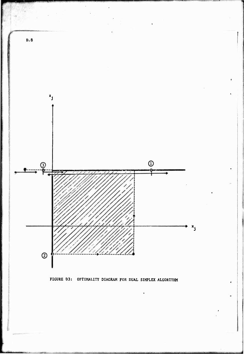
-f

D.8

♦ x.

FIGURE 03: OPTIMALITY DIAGRAM FOR DUAL SIMPLEX ALGORITHM

■,l1" ^ '

*

D.9 1- Forcing x to leave the basis In one pivot may cause "overshooting" in the

sense that some basic variable in B may become primal Infeaslble in B~ , and

hence a future candidate to leave the basis; however, convergence is argued on the

increase In the dual functional D which is equal to the shaded area in Figure

D3. As In the primal simplex algorithm, special rules of choice, such as the

"most nonconforming" (smallest x < 0), or "greatest shaded area" can be used.

E. The Artificial Constraint

The dual simplex method is usually applied because a dual-feasible basis is

known, as in parametric problems. However, if a basis B is known which is

not dual-feasible, then an artificial constraint

5" x. + x - M

may be added, with x a slack activity. This gives an optimality diagram for

x which looks like Figure (D4a) with an enlarged basis for the extended problem

of B0 + {0} .

mm~

D.10

4 1

? I

CO

i 3 u M

M

to

Q

I ■S

cd >

« rH

Nv

1

Now among the non-dual-feasible activities Ji j ^ B , there is one which is

"highest" above line B in Figure D4b, i.e., some k for which

zk- ck- Max [Zj - Cj] .

JeB0

D.ll

(D10)

Vcj

By pivoting on x, in (D9) , all of these points are made conforming on L ,

with x, replacing x in the now dual-feasible extended basis

BD - B0 + {k} (DID

at level

M .

Unless x comes back into the basis at a positive level, the optimal solution

may be unbounded.

F. The Primal-Dual Method

In the primal dual-method [7], one begins with a (not necessarily basic)

dual feasible solution {y^} , and a primal in which nonnegative artificial

variables x have been added to every primal constraint. This gives the

•j optiroallty diagrams shown In Figure D5a and b.

■i ^^^^^■^»^—^—.

D.12

i i

T

I

r-<-4

t

ift a) M

•H u >

(0

^

Q o

i Ö

I

N 4- M ft! a, w

±

O tu

Ö

en

«

u

>

>> M n) c

•H T) M O

o

Q

W

O M tu

D,13

The Initial starting solutions arc the nonbasic variables x = 0 , and

basic variables x = bJ (note that z ^ y,) •

If z. < c. , then all such variables are "frozen" in L ; only variables for

which z ■ c are allowed to vary in an associated restricted primal. The

objective of this general linear programming problem is to minimize the error

terms:

(D12) Minimize E = ^ x aj

while keeping all ordinary variables conforming (in L or B). When E = 0 ,

the optimal solution is obtained.

This method can be directly explained as a special case of the algorithm of

Section 6, when applied to nonnegative unbounded variables.

(a) The indices of the artificial variables are taken as the set J ;

+ these variables are nonconforming in L

(b) The ordinary variables are considered to be conforming in L If

z. - c. < 0 , or in B if z. » c. .

(c) In applying the incremental subroutine, all nonconforming (artificial)

variables are worked on simultaneously (e. ■ - 1 for J nonconforming)

Otherwise, the primal-dual algorithm is identical to our algorithm with no

special freezing or one-pivot rules being used (except possibly between artificial

variables only), Successive applications of the incremental subroutine will

reduce the artificial variables, following the usual breakpoint-stepping procedure,

and the optimal solution to the restricted problem after one pass can be used as

the starting solution for the next pass (the optimal J from one pass can be

used to start the next one).

As is well known, in certain problems one may avoid putting in artificial

D.1A

variables for all constraints; for example, in flow problems, the conservation

equations are never violated, since each (incremental) maximal flow subroutine

only adds loop flows. Also, for this class of problems the subroutine Is solved

by a particularly efficient labelling algorithm.

If no dual-feasible solution exists, then an artificial constraint

(D13)

is added, and

11

I x. + 1=1 ■*

x = M o

(DU)

min [0. c ) J 2

1, m

constitutes a dual-feasible solution to the augmented program.

G. Cost Parametrization

If a certain unit cost, c , is to be studied parmetrically, starting from

an optimal solution (x ; z.) , then the substitution

(D15) CJ " CJ + e

is made with, say, increasing values of 9 . The optimality diagram for this

activity moves upward by an amount 6 , leaving the current solution (x,; z ) « j j

either conforming in L(x. =0) , or nonconforming in L (x. > 0) . (Figure D6)

-

D.15

«

■J

c;.cJ + e- ■

t0 - c i ■ \

J CJ

0 *\

FIGURE D6: OPTIMALITY DIAGRAM FOR COST PARAMETRIZATION

D.16

In the first case, 6 can increase without limit, activity j remaining

nonbasic in L , with no change in C -Z> .

In the second case, J is the only nonconforming activity, so the subroutine

seeks to minimize ^ , keeping all other activities conforming. After a possible

* finite decrease in x. equal to -A. at level c , a dual change is made, moving

* the current solution upwards by an amount 9. , then to the left by an amount

-&„, ..., etc., following the familiar breakpoint curve. Finally, after a finite i

number of steps, the solution will be at the desired level z = c. , or x. = 0 .

Because the starting solution was optimal, except for J , only one basis change

will usually be made in the subroutine as an activity in L changes to B or

vice versa (except for degeneracy).

fi * In the familiar tracing-out of the piecewisc linear curve of t- versus

6 , the vertical displacements Q-i»®?' ■,■' etc' » corresPond t0 intervals between

tuvnxrvg "points of C % and the determination of A corresponds to the basis

change at these turning points. The decrease in *£> at the origin 0 = 0 is

-A-, (c. - z.) , and the increase in C when 9 changes to 9. is 9., (x + A.) ,

etc.

Complementary remarks apply to a decrease in 0

If a vector change in the c is proposed:

(D16) c3 " cj + eej

j • 1,2, ..., n

then the several nonconforming activities are worked upon at the same time by

the incremental subroutine with e - -e. .

H. Right-Hand Side Parametrization

First, suppose some requirements value, b. , is to be changed to:

(D17) bi = bi + *

o . o starting from an optimal solution (x Jz.) . The corresponding equality constraint

can again be satisfied by adding an artificial variable x at level

x = b. - b. : ail

(D18) ^ 'ij XJ + X- ■ bi '

This variable Is now non con forming with z = y. , as shown in Figure D7a.

D.17

mm

D.18

x 11

o A " ■e-

o

o 2 ■ - o

0» I u

cr c

o

I

r •

n

«a N

r -*-d O -H

4- -►—I

r I

4

•

o id

i u

c 0)

l-l

3 cr v

Q

H

O

Q

W

Ü M

Since this is the only nonconforming var iable , s uccessive applications of the

algorithm will always be minimizing ( , and the dual variable a will

D.l9

increase as x decreases ( ~increases). Horizontal displacements correspond a

* * to changes in ~ , while vertical displacements cause changes in ~ , while

(y1

; ~) traces out the familiar breakpoi nt curve.

If the right-hand side change is in an inequality,

(Dl9)

with 0 xj > 0 , then no change will occur for positive, j remaining in B

(Fi gure D7b ). However, for some negative ~ , j will become nonconforming in

B+ , and a breakpoint curve similar to the requirements change above must be traced out.

Obvious remarks apply to vector changes in the {bi} , changes in some ij ,

et c . (SeE: also Section 9.)

I. Composite Methods

In the composite methods, such as he self-dual parametric algorithm [5] ,

or the composite algorithm [13] one permits a starting solution with a basis B0

in wh ich both

(D20) 0 xj < 0 for some (possibly all) ("primal-infeasible" )

(D21) z; > .cj for some (possibly all) j t B0 ("dual-infeasible").

By a combination of the parametric methods of the last two paragraphs:

(a)

and (b)

0 Setting x ai

the activity

• x; , and xj • 0 in equation i

j in (D20), and then driving all

corresponding to

x to zero; ai

Increasing cj temporarily to the level 0 zj , and then decreasing

all of them parametrically to zero, for all j in (D21).

D.20

one can, it is explained, always work with a primal-and-dual-feasible basic

solution and proceed to the optimum "by successive application of either the

primal or dual simplex rules." (Subsection A and C.) These parametric changes

can all be worked on simultaneously, or one at a time (usually Ignoring the

others).

A much simpler explanation is given in terms of the optimality diagram.

Because a basic solution is always given, the nonconforming activities are

either in B or have (z. > c and x = 0) (Figure D8). Application of the

algorithm takes B for «i , and always tries to increase ^ for all j in

(D20) and (D21), either one at a time, or simultaneously. Wolfe [15] gives some

suggestions for efficient choice of the e , based on computational experience.

A composite method is also described by Ballnski and Gomory [2], which avoids

degeneracy through a hierarchy of "sub-primal" and "sub-dual" tableaux.

_^.

D.21

Dual Infeasible

r

.

' ~--------------------

Primal- InfE lasible

f -__..

0

FIGURE D8: OPTIMALITY DIAGRAM IN THE COMPOSITE METHODS

•

■^■W^^PP"

)

E.l

APPENDIX E. AN EXAMPLE

As an example of the COMPLEX approach, consider the following program

Mln (? = 2 max (0, x - 1) + 2 x. - x

Xl + 2 x2 + x3 > 2

x. + 6 x- + 5 x_ = - 4

0 1 "i 1 3r " 1 x2 i ■*"2; lx3l 1 * •

We add variables x, and x,. to the constraints, together with the bounds

Max C • J - {A,5} . After two zero-level pivots, x increases to Its

* * 1 corner point, increasing x,. , and decreasing x, . A ■ 2 • 6 ■ -r 1« limitec

by the downward movement x. • J[ - {2,3} . Activity #3 is now conforming

and take the simple (but poor) starting solutions

x0 - (0, 0, 0, 2, -A)

y0 - (0, 0) C0 - d0 - 0 - 2M + A + 2M + 4M - 8M + A

z0 - (0, 0, 0, 0, 0)

Only activity 91 is initially conforming. The optimality diagrams are shown in

Figure El; note that no prior manipulation of the problem is needed to draw

these diagrams.

The following steps represent a possible sequence of iterations following

a COMPLEX procedure; the appropriate breakpoint trajectories are shown in Figure El.

Iteration 1:

E.2

^* = (1, -^ . 0, 0, 2); i* = (2, 0.- 2, 3, - 1)

x1 - (1, - | , 0. J, 2); z1 - (1. 0, - 1, 3/2, - |)

y1^ (3/2. -|); C1 " ^ = 6M .

Iteration 2:

Max ^ . A zero-level pivot leads to ä" = 0 and the new basis

J = {3, 5} . 6 = T" Is limited by the upward movement of x to a corner point.

C* = (0, 0, 0. 0. 0. 0); c* - (4, A, 0, 5, - 1)

x2 = x1 ; z2 = (2, 1, - 1. ^, - 3/4)

y2 - (^.- 3/A) ; C2 - J2 = 5M .

Iteration 3;

Max Cc • Increasing x drives activity #5 conforming, with A - 2 . Since

all components of c are zero, 6 may take on any value, but does not effect

53 . J3 - {1,3} .

t* - (|, 0, - \t 0, 2); ;* - (0, 0, 0, 0, 0)

x3 - (3/2, -f. -y. 2, 0); z3- z2

y3" (^. -3M); C^-tf ' 3M •

Iteration A:

Min C, • Decreasing x, increases x. to its new corner point, also de-

creasing x-. A - - 6/5 , and J « {3,A) . 6 - 5/A is limited only by the

upward movement of x« into a conforming state

T

E.3

* 3 6 * IL L l\ t - (3/2, 0. - -^ . - I . 0); ? = U' V 0' !• " 5)

U 14 4 U * - (3. - j. - f. f. 0) J z «= (3, 2. - 1, A. - 1)

yA= (A. - 1); C4- 0A=lM •

Iteration 5;

Mln C/ • IncreaslnR x decreases both x„ and x , with & = - 4/5

as activity //4 becomes conforming. «\ ={2,3}. There are no dual changes:

C* - (0, 1, - 6/5. - A/5, 0); q* = (0. 0, 0, 0, 0)

x5 = (3. 4. - 2, 0, 0) 5 4 z = z (3, 2, - 1, 4, - 1) .

Since all states are now conforming, the above solutions are optimal, with

y5 - yA - (A, - 1) and C5 - ft5 " 0 .

Note, In particular, that the trajectories in conforming states need not

be always in the same direction; indeed, they may sometimes pass through the

same corner point several times.

w^ mmmmmmamm

E.4

es in

- - CM

©

©

"cr

0

i

©

© 1

©H 0 0

H ►

ro cv» ^

. . •*

CO

.. «s

m

■- CM

-- H

© ©

<«—■♦■ O W

I ,

CM I

I

I

©

Q

I ■-

0© W

7 ©

1©I

© © © I 4 • 4 ■ ■■ i

©

© t ©

Ir^l I I en CM

V3

I*© r:

ft o

M

Unclassified

Security Classification

DOCUMENT CONTROL DATA • R4D fSecurifv clmuailicaUott ol till«, body at nbitracl and indexing mnnotatton must be enlertd when thm overs// report IM clmtilfted)

I Onir.lNATIN 0 ACT|U|T V (Corporate author)

University of California, Berkeley

2« BCPOBT »ECURI TY CLASSIFICATION

Unclassified 26 CROUP

J REPORT TITLE

A COMPLEMENTARY SLACKNESS, OUT-OF-KILTER ALGORITHM FOR LINEAR PROGRAMMING

4 DESCRIPTIVE NOTES (Tvpt ol »port and Inclutiv* daft)

Research Report S AUTNORCS) d-AX nam*. Ural name. Initial)

JEWELL, William S.

6 REPORT DATE

March 1967 7« TOTAL NO OF PACES

90 76. NO. or neri

16 8« CONTRACT OH CRANT NO.

Nonr-222(83) 6 PROJECT NO

NR 0A7 033 C

Research Project No.: RR 003 07 01

9« ORIOINATOR'S REPORT NUMBERCSJ

0RC 67-6

• 6 OTHER REPORT NOfS; (A ny otharnumbara that may ba attlftad Ihla raporl)

10 AVAILABILITY/LIMITATION NOTICES

Distribution of this document is unlimited.

n SUPPLEMENTARY NOTES Also supported by the Nat'1.Sei.Found, under Grant GP-7A17, and the U.S. Army Res. Office- Durham, Contract DA-31-12A-ARO-D-331.

12 SPONSORING MILITARY ACTIVITY

MATHEMATICAL SCIENCE DIVISION

II ABSTRACT

SEE ABSTRACT

DD .fÄ 1473 Unclassified Security Classification

.—_—.^

f Unclasslfled Security Classification

«« KEY WORDS

Linear Programming

Out-of-kilter

Complementary pivot

Primal-dual

Complementary slackness

LINK A

ROLE

LINK e

ROLt

LINK C

INSTRUCTIONS

1 ORIGINATING ACTIVITY: Enter the name and address of the contractor, subcontractor, granlcr. Department of De- fenae activity or other organization (corporate author) issuing the report.

2a. REPORT SECUHTY CLASSIFICATION: Enter the over- ell aecurity classification of the report. Indicate whether "Reatrictcd Data" is included. Marking is to be in accord- ance with appropriate security regulations.

2b. GROUP: Automatic downgrading is specified In DoD Di- rective 5200.10 and Armed Forces Industrial Manual. Enter the group number. Also, when applicable, ahow that optional markings have been used for Group 3 and Group 4 as author- ized.

3. REPORT TITLE: Enter the complete report title in all capital letters. Titles In all cases should be unclassified. If a meaningful title cannot be selected without classlfica- tiun, show title classification in all capitals in parenthesis immediately following the title.

4. DESCRIPTIVE NOTES: If appropriate, enter the type of nport. e.g., interim, progress, summary, annual, or final. Give the inclusive dates when a specific reporting period Is coveted.

5. AUTHOR(S): Enter the name<s) of authoKs) as shewn on or in the report. Enter Isst nsme, first nsme, middle initial. If xititary, show rank and branch of service. The name of the principal a.ithor is an absolute minimum requirement

6. REPORT DAT£: Enter the date of the report as day, month, year; or month, year. If more than one date appears on the report, use date of publication.

7a. TOTAL NUMBER 0«? PAGES: The total page count should follow normal pagination procedures, i.e., enter the number of pages containing Information.

7b. NUMBER OF REFERENCES: Enter the total number of references cited in the report.

8a. CONTRACT OR GRANT NUMBER: If appropriate, enter the applicable number of the contract or grant under which the report was written.

8b, a , & 8d. PROJECT NUMBER: Enter the appropriate military department identification, auch as project number, sufaproject nuntoer, system numbers, task number, etc.

9a. ORIGINATOR'S REPORT NUMBER(S): Enter the offi- cial report number by which the document will be identified and controlled by the originating activity. Thia number must be unique to this report. 96. OTHER REPORT NUMBER(S): If the report hss been assigned any other report numbers (either by «ha originator or b th ; a, ttsor), also enter this number(s).

10. AVAILABILITY/LIMITATION NOTICES: Enter any lim- itations on further dissemination of the report, other than those

imposed by aecurity classification, using standard statements such as:

(1) "Qualified requesters may obtain copies of this report from DDC"

(2) "Foreign announcement and dissemination of this report by DDC is not authorized."

(3) "U. S. Government agencies may obtain copies of this report directly from DDC. Other qualified DDC users shall request through

ii

(4) "U. S. military agencies may obtain copies of this report directly from DDC Other qualified users shall request through

(5) "All distribution of this report is controlled. Qual- ified DDC users shall request through

If the report has been furnished to the Office of Technical Services, Department of Commerce, for sale to the public, indi- cate this fact and enter the price, if known.

11. SUPPLEMENTARY NOTES: Use for sdditlonol explana- tory notes.

12. SPONSORING MILITARY ACTIVITY: Enter the name of the departmental project office or laboratory sponsoring (pay- ing lor) the research and development Include address.

13. ABSTRACT: Enter sn abstract giving a brief and factual summary of the document indicative of the report, even though it may also appear elsewhere in the body of the technics I re- port. If additional spsce is required, a continuation sheet shall be attached.

It is highly desirable that the abstract of classified reports be unclassified. Esch paragraph of the abstract shall end with an indication of the military security classification of the in- formation in the paragraph, represented as (TS). (S), (C), or (U)

There is no limitation on the length of the abstract. How- ever, the auggested length is from 150 to 225 words.

14- KEY WORDS: Key words are technically meaningful terms or short phra.es that characterize a report and may be used ss indes entries for cataloging the report. Key words must be selected so that no security classification is required. Identi- fiers, such as equipment model designation, trade name, military project code name, geographic location, may be used ss key words but will be followed by an indication of technical con- text. The assignment of links, roles, snd weights is optional.

DD Mfi*.< 1473 (BACK) i

Unclassified Security Classification