Competition After Unbundling: Entry, Industry Structure and Convergence George Ford Chief Economist...
65
-
Upload
margery-bond -
Category
Documents
-
view
216 -
download
1
Transcript of Competition After Unbundling: Entry, Industry Structure and Convergence George Ford Chief Economist...


Competition After Unbundling: Competition After Unbundling: Entry, Industry Structure and Entry, Industry Structure and ConvergenceConvergence
George FordGeorge FordChief EconomistChief EconomistPhoenix CenterPhoenix Center

Basic Setup:Basic Setup:Equilibrium Industry StructureEquilibrium Industry Structure
Firms enter only if they make a profitFirms enter only if they make a profit Entry stops when “the next firm” Entry stops when “the next firm”
expects a negative profitexpects a negative profit When entry stops, the existing When entry stops, the existing
number of firms is the equilibrium number of firms is the equilibrium number of firms (number of firms (NN*)*) No incentive to enterNo incentive to enter No incentive to exitNo incentive to exit

Formal TheoryFormal Theory
ES
N
*
N* = Equilibrium Number of Firms (symmetric) = Weakness of CompetitionS = Market Size in Expenditure (isoelastic demand)E = Sunk Entry Costs
Sources: Sutton, Duvall and Ford (PP10), Beard and Ford
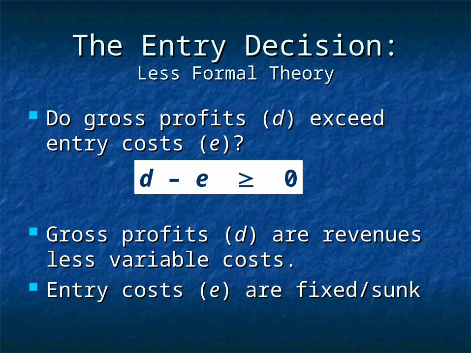
The Entry Decision:The Entry Decision:Less Formal TheoryLess Formal Theory
Do gross profits (Do gross profits (dd) exceed entry ) exceed entry costs (costs (ee)?)?
Gross profits (Gross profits (dd) are revenues less ) are revenues less variable costs.variable costs.
Entry costs (Entry costs (ee) are fixed/sunk) are fixed/sunk
d – e 0

What it MeansWhat it MeansTimeTime RevenueRevenue Discount Discount
FactorFactorDiscounteDiscounte
d d RevenuesRevenues
Entry Entry CostsCosts
00 1.001.00 $500.00 $500.00
11 $100.00 $100.00 0.910.91 $90.91 $90.91
22 $100.00 $100.00 0.830.83 $82.64 $82.64
33 $100.00 $100.00 0.750.75 $75.13 $75.13
44 $100.00 $100.00 0.680.68 $68.30 $68.30
55 $100.00 $100.00 0.620.62 $62.09 $62.09
66 $100.00 $100.00 0.560.56 $56.45 $56.45
77 $100.00 $100.00 0.510.51 $51.32 $51.32
88 $100.00 $100.00 0.470.47 $46.65 $46.65
99 $100.00 $100.00 0.420.42 $42.41 $42.41
1010 $100.00 $100.00 0.390.39 $38.55 $38.55
SumSum $614.46 $614.46 $500.00 $500.00

Want Facilities-based Entry?Want Facilities-based Entry?
Increase Gross ProfitsIncrease Gross Profits
Reduce Entry CostsReduce Entry Costs
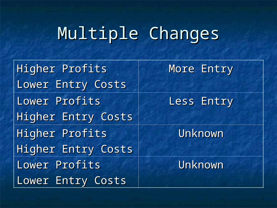
Multiple ChangesMultiple Changes
Higher ProfitsHigher Profits
Lower Entry CostsLower Entry CostsMore EntryMore Entry
Lower ProfitsLower Profits
Higher Entry CostsHigher Entry CostsLess EntryLess Entry
Higher ProfitsHigher Profits
Higher Entry CostsHigher Entry CostsUnknownUnknown
Lower ProfitsLower Profits
Lower Entry CostsLower Entry CostsUnknownUnknown
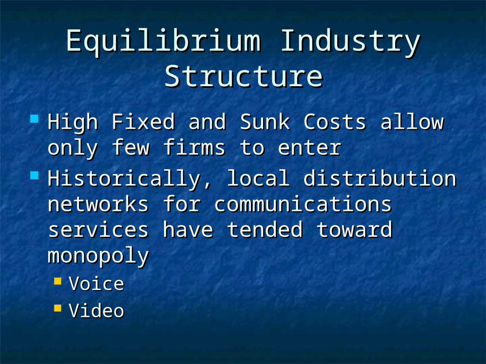
Equilibrium Industry Equilibrium Industry StructureStructure
High Fixed and Sunk Costs allow only High Fixed and Sunk Costs allow only few firms to enterfew firms to enter
Historically, local distribution Historically, local distribution networks for communications networks for communications services have tended toward services have tended toward monopolymonopoly VoiceVoice VideoVideo
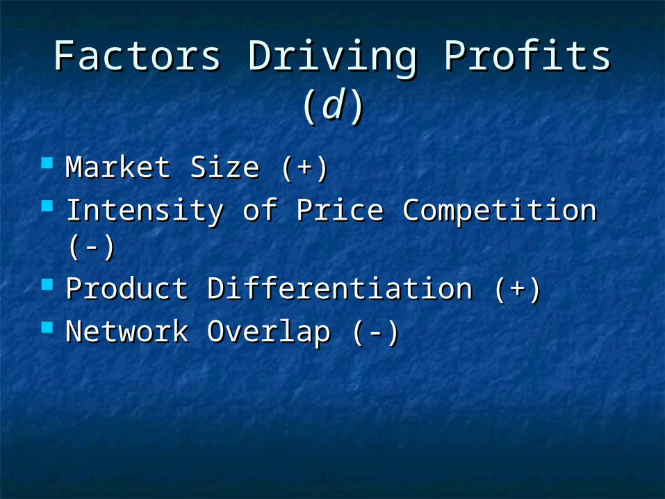
Factors Driving Profits (Factors Driving Profits (dd))
Market Size (+)Market Size (+) Intensity of Price Competition (-)Intensity of Price Competition (-) Product Differentiation (+)Product Differentiation (+) Network Overlap (-)Network Overlap (-)

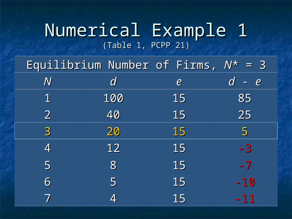
Numerical Example 1Numerical Example 1(Table 1, PCPP 21)(Table 1, PCPP 21)
Equilibrium Number of Firms, Equilibrium Number of Firms, NN* = 3* = 3
NN dd ee dd - - ee
11 100100 1515 8585
22 4040 1515 2525
33 2020 1515 55
44 1212 1515 -3-3
55 88 1515 -7-7
66 55 1515 -10-10
77 44 1515 -11-11

Numerical Example 2Numerical Example 2(Higher Gross Profits)(Higher Gross Profits)
Equilibrium Number of Firms, Equilibrium Number of Firms, NN* = 5* = 5
NN dd ee dd - - ee
11 200200 1515 185185
22 8080 1515 6565
33 4040 1515 2525
44 2424 1515 99
55 1616 1515 11
66 1010 1515 -5-5
77 88 1515 -7-7

Factors Driving Profits (Factors Driving Profits (dd))
Market Size (+)Market Size (+) Intensity of Price Competition (-)Intensity of Price Competition (-) Product Differentiation (+)Product Differentiation (+) Network Overlap (-)Network Overlap (-)

Numerical Example 3Numerical Example 3(Intensity of Price Competition)(Intensity of Price Competition)
NN ee Intense Price Intense Price CompetitionCompetition
Moderate Moderate Price Price
CompetitionCompetition
PerfectPerfect
CollusionCollusion
dd d - ed - e dd d - ed - e dd d - ed - e
11 1515 100100 8585 100100 8585 100100 8585
22 1515 2828 1313 4040 2525 5050 3535
33 1515 1212 -3-3 2020 55 3333 1818
44 1515 66 -9-9 1212 -3-3 2525 1010
55 1515 44 -11-11 88 -7-7 2020 55
66 1515 33 -12-12 55 -10-10 1717 22
77 1515 22 -13-13 44 -11-11 1414 -1-1

Headcount and CompetitionHeadcount and Competition
With large fixed/sunk costs, With large fixed/sunk costs, headcounts can be deceivingheadcounts can be deceiving A large number of firms may indicate A large number of firms may indicate
collusioncollusion A small number of firms may indicate A small number of firms may indicate
intense price competitionintense price competition

Entry and CollusionEntry and Collusion(Based on Post-Convergence Example Above)(Based on Post-Convergence Example Above)
Firm 1Firm 1
EnterEnter Stay OutStay Out
Firm 2Firm 2
EnterEnter 5050
50504040
110110
Stay OutStay Out 110110
4040100100
100100

Factors Driving Profits (Factors Driving Profits (dd))
Market Size (+)Market Size (+) Intensity of Price Competition (-)Intensity of Price Competition (-) Product Differentiation (+)Product Differentiation (+) Network Overlap (-)Network Overlap (-)

Product Differentiation and Product Differentiation and OverlapOverlap
Price
Homes/Overlap50% 100%
P1
P2
P3
More Differentiation
Less Differentiation
Differentiation weakens price competition.
Overlap increases price competition.
Phoenix Center Policy Paper No. 21, Figure 1.
Diversion:Diversion:Competition and SubstitutionCompetition and Substitution
Competition occurs between Competition occurs between goods/services that perform a similar goods/services that perform a similar task for consumerstask for consumers
Good X is a substitute for Good Y if Good X is a substitute for Good Y if the the demanddemand for Good X rises when for Good X rises when the the priceprice of Good Y rises (and vice of Good Y rises (and vice versa)versa)
Diversion:Diversion:Competition and SubstitutionCompetition and Substitution
The relationship of quantities of goods The relationship of quantities of goods is not an indicator of substitutionis not an indicator of substitution Unless we already know the goods are Unless we already know the goods are
perfect substitutesperfect substitutes Substitution is of degreeSubstitution is of degree
Airplanes, Buses, Cars, Trains all provide Airplanes, Buses, Cars, Trains all provide transportation, but we might be concerned transportation, but we might be concerned about a monopoly over any of one of themabout a monopoly over any of one of them

Diversion:Diversion:Competition and SubstitutionCompetition and Substitution
As long as the own-price demand As long as the own-price demand elasticity is less than –1.0 (or inelastic), elasticity is less than –1.0 (or inelastic), then a 5% price increase is profitablethen a 5% price increase is profitable
Cross-price elasticities are not Cross-price elasticities are not indicators of Antitrust marketsindicators of Antitrust markets Large cross price elasticities are indicators Large cross price elasticities are indicators
of good substitution, but if own-price is not of good substitution, but if own-price is not elastic enough, a significant price increase elastic enough, a significant price increase remains profitableremains profitable

ExampleExample
Wireless Substitution and CompetitionWireless Substitution and Competition, by Stephen , by Stephen PociaskPociask
lnlnQQMM = -0.56 = -0.56 ·· ln lnPPMM + 1.97 + 1.97··lnlnPPWW++X+X+ More wrong with the econometrics of this paper than I
could cover in a day, much less an hour “…the models provide compelling empirical evidence
that wireless and wireline services are indeed substitute goods, and are not extraneous or complementary goods (at 15).”
This model indicates substitution (an implausibly large amount of it), but still not enough substitution to place wireless/wireline in the same market.
Q is quantity, P is price, M is mobile, W is wireline, ln is the nat. logarithmic transformation, X is the means of the other variables in the model multiplied by their coefficients.
Types of Entry Costs (Types of Entry Costs (ee))
Technological Entry Costs (+)Technological Entry Costs (+) Strategic Entry Costs (+)Strategic Entry Costs (+) Regulatory Entry Costs (+)Regulatory Entry Costs (+) Spillovers (-)Spillovers (-)

Types of Entry Costs (Types of Entry Costs (ee))
Technological Entry Costs (+)Technological Entry Costs (+) Entry costs that are unavoidable to Entry costs that are unavoidable to
provide serviceprovide service NetworkNetwork Operating CapitalOperating Capital AdvertisingAdvertising Building LeasesBuilding Leases Etc…Etc…

Types of Entry Costs (Types of Entry Costs (ee))
Strategic Entry Costs (+)Strategic Entry Costs (+) Entry costs that arise solely because of Entry costs that arise solely because of
incumbent firm actions intended to raise incumbent firm actions intended to raise entry costsentry costs
Excessive AdvertisingExcessive Advertising Lock-in ContractsLock-in Contracts Strategic PricingStrategic Pricing
Types of Entry Costs (Types of Entry Costs (ee))
Regulatory Entry Costs (+)Regulatory Entry Costs (+) Rules that raise entry costs above Rules that raise entry costs above
technological entry coststechnological entry costs Build-out RequirementsBuild-out Requirements Gold-plating NetworksGold-plating Networks Entry FeesEntry Fees E911 and other social programsE911 and other social programs
If socially-desirable, there may be a trade-off If socially-desirable, there may be a trade-off between entry and the provision of the service between entry and the provision of the service (e.g., E911)(e.g., E911)

Types of Entry Costs (Types of Entry Costs (ee))
Spillovers (-)Spillovers (-) Spillovers exist when a firm can use Spillovers exist when a firm can use
existing assets to enter related markets.existing assets to enter related markets. This firm has lower entry costs than a This firm has lower entry costs than a
firm without existing assets that can be firm without existing assets that can be leveraged into a related marketleveraged into a related market
Network (DSL over Copper; Cable Broadband Network (DSL over Copper; Cable Broadband over Coax; Fiber over existing rights-of-way; over Coax; Fiber over existing rights-of-way; customer relationships)customer relationships)
Numerical Example 1Numerical Example 1(Table 1, PCPP 21)(Table 1, PCPP 21)
Equilibrium Number of Firms, Equilibrium Number of Firms, NN* = 3* = 3
NN dd ee dd - - ee
11 100100 1515 8585
22 4040 1515 2525
33 2020 1515 55
44 1212 1515 -3-3
55 88 1515 -7-7
66 55 1515 -10-10
77 44 1515 -11-11

Numerical Example 4Numerical Example 4(Reduced Entry Costs)(Reduced Entry Costs)
Equilibrium Number of Firms, Equilibrium Number of Firms, NN* = 6* = 6
NN dd ee dd - - ee
11 100100 55 9595
22 4040 55 3535
33 2020 55 1515
44 1212 55 77
55 88 55 33
66 55 55 00
77 44 55 -1-1
Spillovers and ConvergenceSpillovers and Convergence
Convergence is relevant only when it Convergence is relevant only when it reduces entry costs.reduces entry costs.
Effects of convergence are generally Effects of convergence are generally limited to firms with existing assets limited to firms with existing assets that can be “spilled over” into that can be “spilled over” into related markets. related markets.

Numerical Example 5Numerical Example 5(Spillovers and Convergence)(Spillovers and Convergence)
Pre-ConvergencePre-Convergence
Monopoly Monopoly ProfitProfit
Duopoly Duopoly Profit (Profit (dd))
Entry Costs Entry Costs ((ee))
dd – – ee
Market 1Market 1 100100 4040 5050 -10-10
Market 2Market 2 100100 4040 5050 -10-10
Post-ConvergencePost-Convergence
Monopoly Monopoly ProfitProfit
Duopoly Duopoly Profit (Profit (dd))
Entry Costs Entry Costs ((ee))
dd – – ee
Market 1Market 1 100100 4040 3030 1010
Market 2Market 2 100100 4040 3030 1010
No Entry

Equilibrium Industry Equilibrium Industry Structure:Structure:
SummarySummary There will be few local networksThere will be few local networks So, rig the game in favor of entry by So, rig the game in favor of entry by
new firms and expansion by existing new firms and expansion by existing firms into related marketfirms into related market Eliminate regulatory entry barriersEliminate regulatory entry barriers Impede strategic entry barriersImpede strategic entry barriers Expand marketsExpand markets

Phoenix Center Policy Paper Phoenix Center Policy Paper No. 22No. 22
The Consumer Welfare Cost of The Consumer Welfare Cost of Cable “Build-Out” RulesCable “Build-Out” Rules

Build-Out RulesBuild-Out Rules
Unambiguously Bad for EntrantsUnambiguously Bad for Entrants May be good for ConsumersMay be good for Consumers May be good for IncumbentsMay be good for Incumbents But can’t be good for both Consumers But can’t be good for both Consumers
and Incumbents at the same timeand Incumbents at the same time Why do both policymakers and incumbents Why do both policymakers and incumbents
advocate for build-out rulesadvocate for build-out rules??

Build-Out Rule:Build-Out Rule:Graphical ExplanationGraphical Explanation
Price
Homes/OverlapH
homes ordered by capital cost
r(h)
e(h)
e(h): Entry Cost for home ir(h): Expected Revenue for home i
Phoenix Center Policy Paper No. 22, Figure 1.
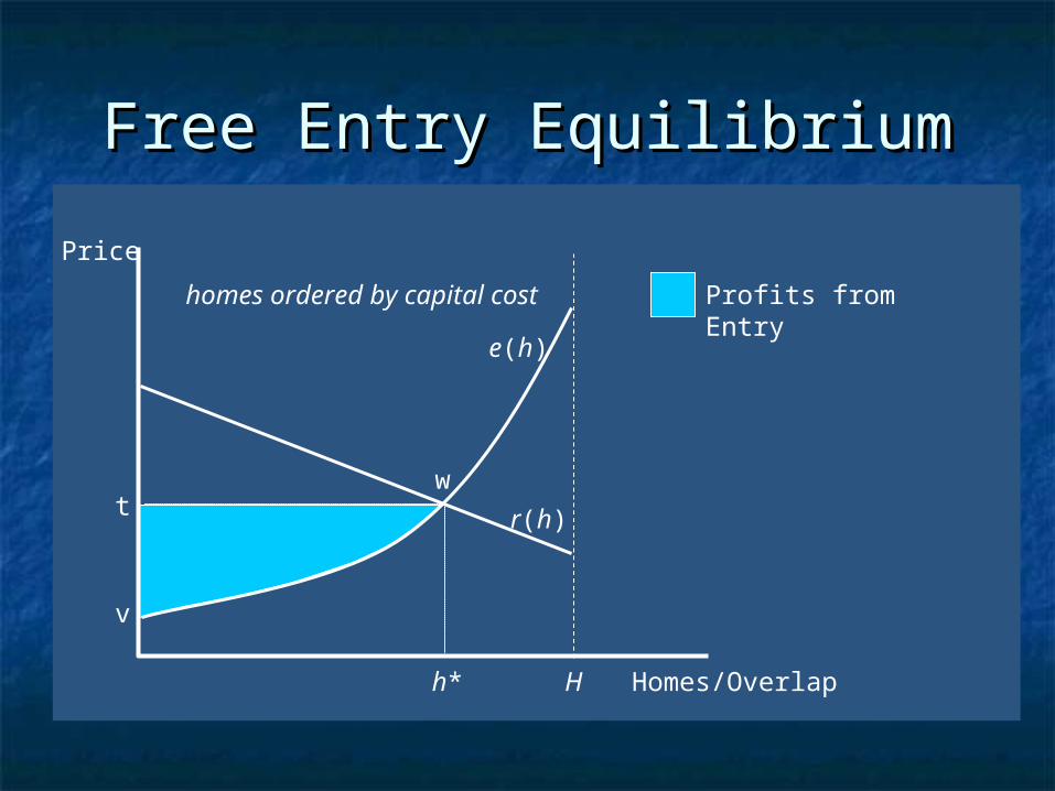
Free Entry EquilibriumFree Entry Equilibrium
Price
Homes/Overlaph* H
homes ordered by capital cost
t
v
w
r(h)
e(h)
Profits from Entry

With Build-Out RuleWith Build-Out Rule
Price
Homes/OverlapH
homes ordered by capital cost
u
v
x
y
z
r(h)
e(h)
Profits from Entry
Losses from Entry
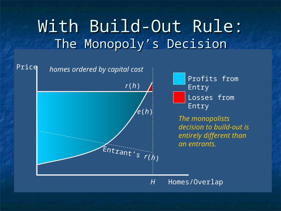
With Build-Out Rule:With Build-Out Rule:The Monopoly’s DecisionThe Monopoly’s Decision
Price
Homes/OverlapH
homes ordered by capital cost
r(h)
e(h)The monopolists decision to build-out is entirely different than an entrants.
Profits from Entry
Losses from Entry
Entrant’s r(h)
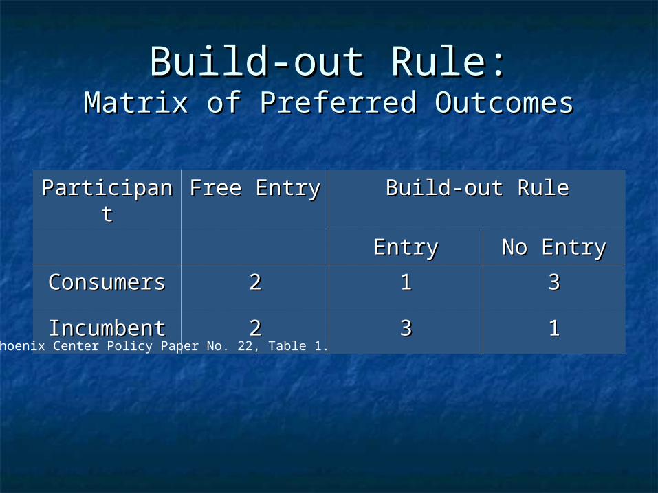
Build-out Rule:Build-out Rule:Matrix of Preferred OutcomesMatrix of Preferred Outcomes
ParticipantParticipant Free EntryFree Entry Build-out RuleBuild-out Rule
EntryEntry No EntryNo Entry
ConsumersConsumers 22 11 33
IncumbentIncumbent 22 33 11
Phoenix Center Policy Paper No. 22, Table 1.
FCC on Build-out RulesFCC on Build-out Rules
““build-out requirements are of central build-out requirements are of central importance to competitive entry importance to competitive entry because these requirements impact because these requirements impact the threshold question of whether a the threshold question of whether a potential competitor will enter the potential competitor will enter the local exchange market at all.” local exchange market at all.” FCC No. FCC No. 97-346 (1997)97-346 (1997)

SimulationSimulation
Summary of ResultsSummary of ResultsEntrantEntrant
H-PassH-PassMarketsMarkets
ServedServedEntrantEntrant
CAPEXCAPEXConsumConsum
er er SurplusSurplus
IncumbenIncumbent Profitt Profit
MonopolMonopolyy
…… …… …… 60M60M 120M120M
Free Free EntryEntry
60,00060,000 100100 18M18M 75M75M 94M94M
Build-outBuild-out 15,00015,000 1515 6M6M 64M64M 113M113MPhoenix Center Policy Paper No. 22, Table 2.Assumptions: Entrant market share = 35%. Price decline for 100% overlap is 20%.
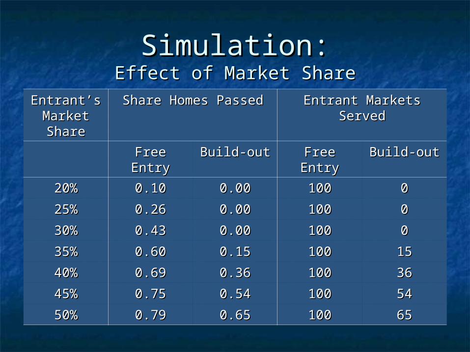
Simulation:Simulation:Effect of Market ShareEffect of Market Share
Entrant’s Entrant’s Market Market ShareShare
Share Homes PassedShare Homes Passed Entrant Markets ServedEntrant Markets Served
Free EntryFree Entry Build-outBuild-out Free EntryFree Entry Build-outBuild-out
20%20% 0.100.10 0.000.00 100100 00
25%25% 0.260.26 0.000.00 100100 00
30%30% 0.430.43 0.000.00 100100 00
35%35% 0.600.60 0.150.15 100100 1515
40%40% 0.690.69 0.360.36 100100 3636
45%45% 0.750.75 0.540.54 100100 5454
50%50% 0.790.79 0.650.65 100100 6565

Simulation:Simulation:Build-out and InvestmentBuild-out and Investment
Entrant’s Entrant’s Market Market ShareShare
Share Homes PassedShare Homes Passed InvestmentInvestment
Free EntryFree Entry Build-outBuild-out Free EntryFree Entry Build-outBuild-out
20%20% 0.100.10 0.000.00 22 00
25%25% 0.260.26 0.000.00 77 00
30%30% 0.430.43 0.000.00 1212 00
35%35% 0.600.60 0.150.15 1818 66
40%40% 0.690.69 0.360.36 2222 1515
45%45% 0.750.75 0.540.54 2626 2323
50%50% 0.790.79 0.650.65 2828 3030
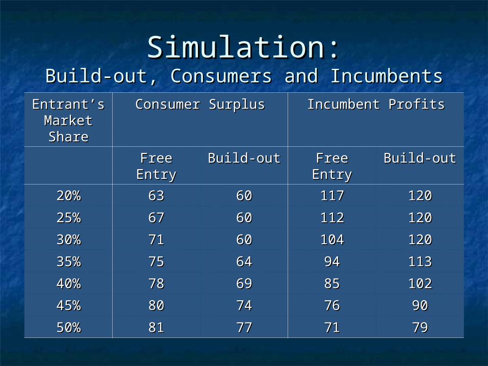
Simulation:Simulation:Build-out, Consumers and IncumbentsBuild-out, Consumers and Incumbents
Entrant’s Entrant’s Market Market ShareShare
Consumer SurplusConsumer Surplus Incumbent ProfitsIncumbent Profits
Free EntryFree Entry Build-outBuild-out Free EntryFree Entry Build-outBuild-out
20%20% 6363 6060 117117 120120
25%25% 6767 6060 112112 120120
30%30% 7171 6060 104104 120120
35%35% 7575 6464 9494 113113
40%40% 7878 6969 8585 102102
45%45% 8080 7474 7676 9090
50%50% 8181 7777 7171 7979

DefectionDefection
What happens if some communities What happens if some communities abandon the build-out rule when others abandon the build-out rule when others maintain it?maintain it? Defection raises the defector’s relative Defection raises the defector’s relative
profitability, increasing the prospects for profitability, increasing the prospects for deployment sooner (rather than later, if deployment sooner (rather than later, if ever)ever)
With 25% defection rates, average increase With 25% defection rates, average increase in profit rank is 38 positions (out of 100)in profit rank is 38 positions (out of 100)

In Defense of Build-out In Defense of Build-out RulesRules
NCTANCTA Incumbent cable firms cross-subsidize Incumbent cable firms cross-subsidize
low value areas with profits from high-low value areas with profits from high-value areasvalue areas
Entry in high-value areas only depletes Entry in high-value areas only depletes source of cross subsidy, threatening source of cross subsidy, threatening upgrades/expansion in low value areasupgrades/expansion in low value areas
Entrants should have to build-out too, Entrants should have to build-out too, regardless of whether it deters entryregardless of whether it deters entry

In DefenseIn DefenseThe Monopoly’s DecisionThe Monopoly’s Decision
Price
HomesH
homes ordered by capital cost
r(h)
e(h)
Profits offset losses forMonopoly build-out.
Profits from Entry
Losses from Entry

In DefenseIn DefenseEntry with Uniform PriceEntry with Uniform Price
Price
Homes/OverlapH
homes ordered by capital cost
r(h)
e(h)
Profits insufficient to cover losses. But, entrant does not enter (50-50 split of the market).
Profits from Entry
Losses from Entry
Entrant’s r(h)
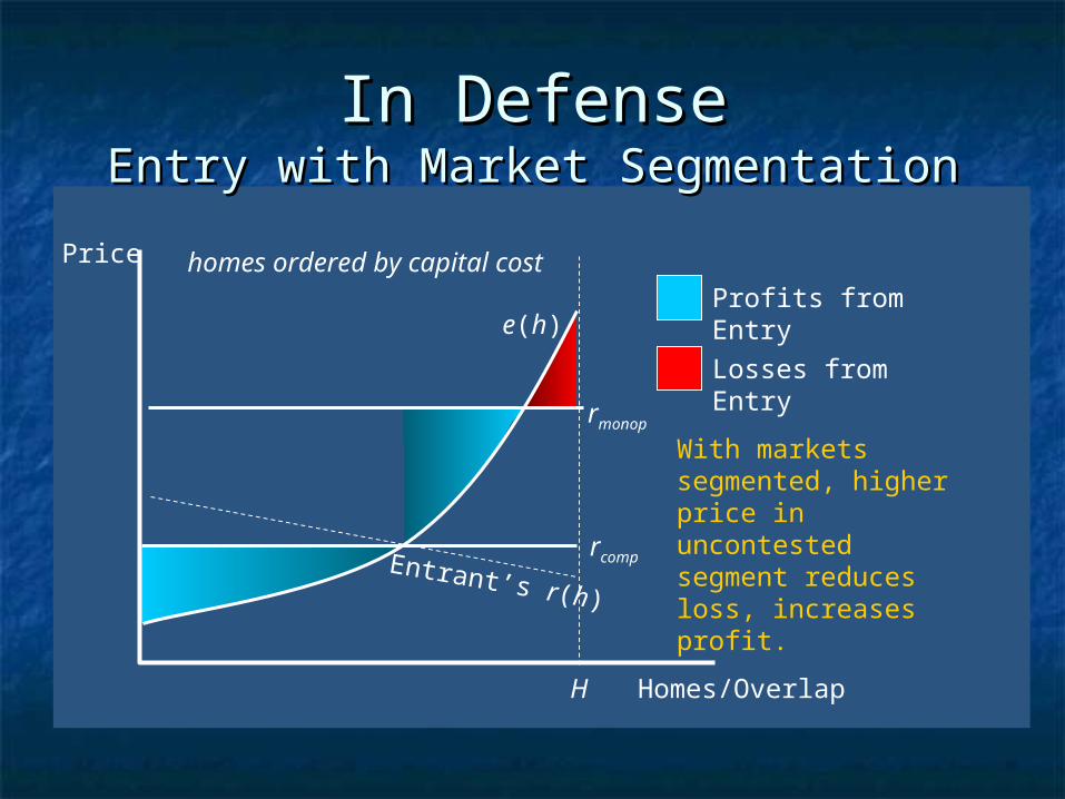
In DefenseIn DefenseEntry with Market SegmentationEntry with Market Segmentation
Price
Homes/OverlapH
homes ordered by capital cost
rcomp
e(h)
With markets segmented, higher price in uncontested segment reduces loss, increases profit.
Profits from Entry
Losses from Entry
Entrant’s r(h)
rmono
p
Evaluation of DefenseEvaluation of Defense
Cable network is sunkCable network is sunk As long as revenues exceed the As long as revenues exceed the
incremental cost of the network incremental cost of the network (programming, maintenance), there is (programming, maintenance), there is no incentive to abandon the networkno incentive to abandon the network
According to NCTA, upgrades are done According to NCTA, upgrades are done at the edge of the network, so initial at the edge of the network, so initial capital cost of network are somewhat capital cost of network are somewhat irrelevantirrelevant
Evaluation: Social GoalEvaluation: Social Goal
NCTA says build-out is a social goalNCTA says build-out is a social goal Build network where we shouldn’t (in a Build network where we shouldn’t (in a
market economy sense)market economy sense) NCTA Solution: NCTA Solution:
Build 2 networks where there shouldn’t Build 2 networks where there shouldn’t be 1be 1
Evaluation: Social GoalEvaluation: Social Goal
Why should buildouts be based on cable Why should buildouts be based on cable franchise markets?franchise markets? Franchise boundaries are arbitrary, not Franchise boundaries are arbitrary, not
economic boundarieseconomic boundaries ILEC territories often don’t matchILEC territories often don’t match
If broadband availability is a function of If broadband availability is a function of video in the bundle, then local video in the bundle, then local governments are interfering with federal governments are interfering with federal role in broadband deploymentrole in broadband deployment
Evaluation: Social GoalEvaluation: Social Goal
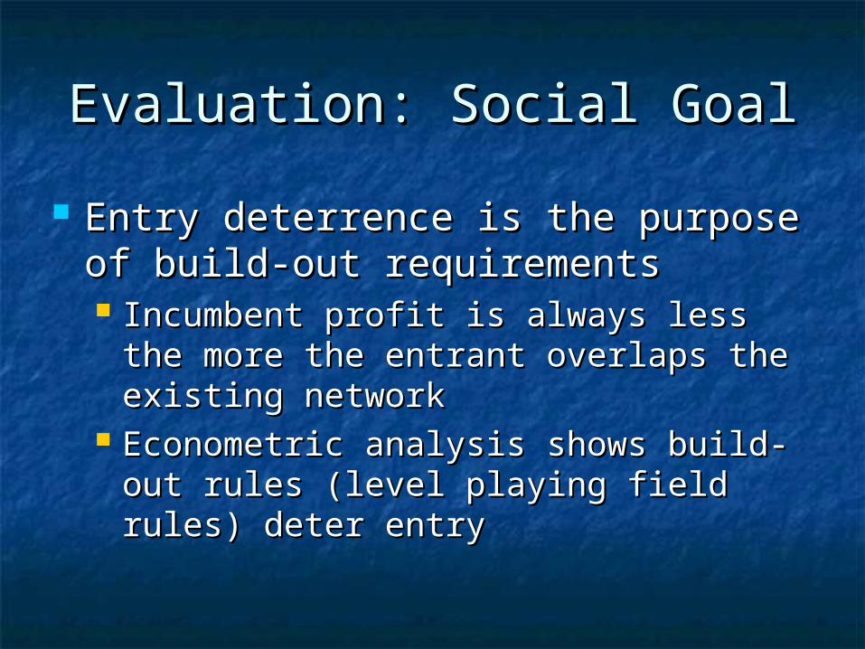
Entry deterrence is the purpose of Entry deterrence is the purpose of build-out requirementsbuild-out requirements Incumbent profit is always less the more Incumbent profit is always less the more
the entrant overlaps the existing the entrant overlaps the existing networknetwork
Econometric analysis shows build-out Econometric analysis shows build-out rules (level playing field rules) deter rules (level playing field rules) deter entryentry

Phoenix Center Policy Paper Phoenix Center Policy Paper No. 23No. 23
Video and Broadband Network Video and Broadband Network DeploymentDeployment

Want Facilities-based Entry?Want Facilities-based Entry?
Increase Gross ProfitsIncrease Gross Profits
Reduce Entry CostsReduce Entry Costs
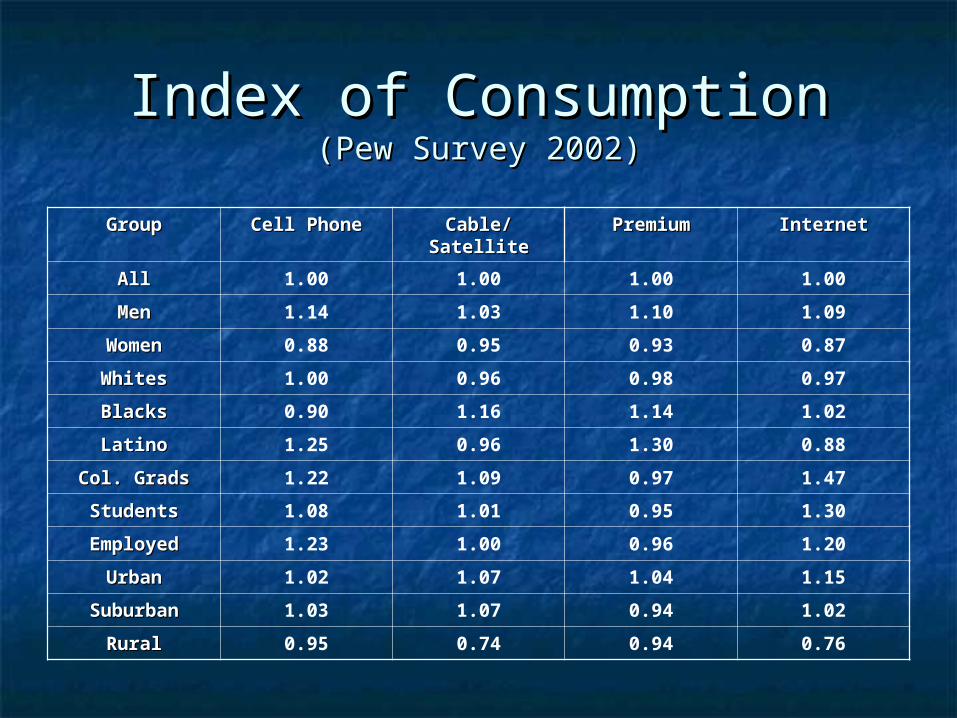
Index of ConsumptionIndex of Consumption(Pew Survey 2002)(Pew Survey 2002)
GroupGroup Cell PhoneCell Phone Cable/Cable/SatelliteSatellite
PremiumPremium InternetInternet
AllAll 1.00 1.00 1.00 1.00
MenMen 1.14 1.03 1.10 1.09
WomenWomen 0.88 0.95 0.93 0.87
WhitesWhites 1.00 0.96 0.98 0.97
BlacksBlacks 0.90 1.16 1.14 1.02
LatinoLatino 1.25 0.96 1.30 0.88
Col. GradsCol. Grads 1.22 1.09 0.97 1.47
StudentsStudents 1.08 1.01 0.95 1.30
EmployedEmployed 1.23 1.00 0.96 1.20
UrbanUrban 1.02 1.07 1.04 1.15
SuburbanSuburban 1.03 1.07 0.94 1.02
RuralRural 0.95 0.74 0.94 0.76
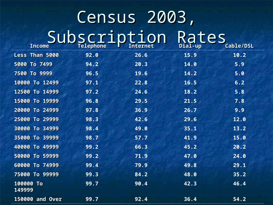
Census 2003, Subscription Census 2003, Subscription RatesRates
IncomeIncome TelephoneTelephone InternetInternet Dial-upDial-up Cable/DSLCable/DSL
Less Than 5000Less Than 5000 92.0 26.6 15.9 10.2
5000 To 74995000 To 7499 94.2 20.3 14.0 5.9
7500 To 99997500 To 9999 96.5 19.6 14.2 5.0
10000 To 1249910000 To 12499 97.1 22.8 16.5 6.2
12500 To 1499912500 To 14999 97.2 24.6 18.2 5.8
15000 To 1999915000 To 19999 96.8 29.5 21.5 7.8
20000 To 2499920000 To 24999 97.8 36.9 26.7 9.9
25000 To 2999925000 To 29999 98.3 42.6 29.6 12.0
30000 To 3499930000 To 34999 98.4 49.0 35.1 13.2
35000 To 3999935000 To 39999 98.7 57.7 41.9 15.0
40000 To 4999940000 To 49999 99.2 66.3 45.2 20.2
50000 To 5999950000 To 59999 99.2 71.9 47.0 24.0
60000 To 7499960000 To 74999 99.4 79.9 49.8 29.1
75000 To 9999975000 To 99999 99.3 84.2 48.0 35.2
100000 To 100000 To 149999149999
99.7 90.4 42.3 46.4
150000 and 150000 and OverOver
99.7 92.4 36.4 54.2
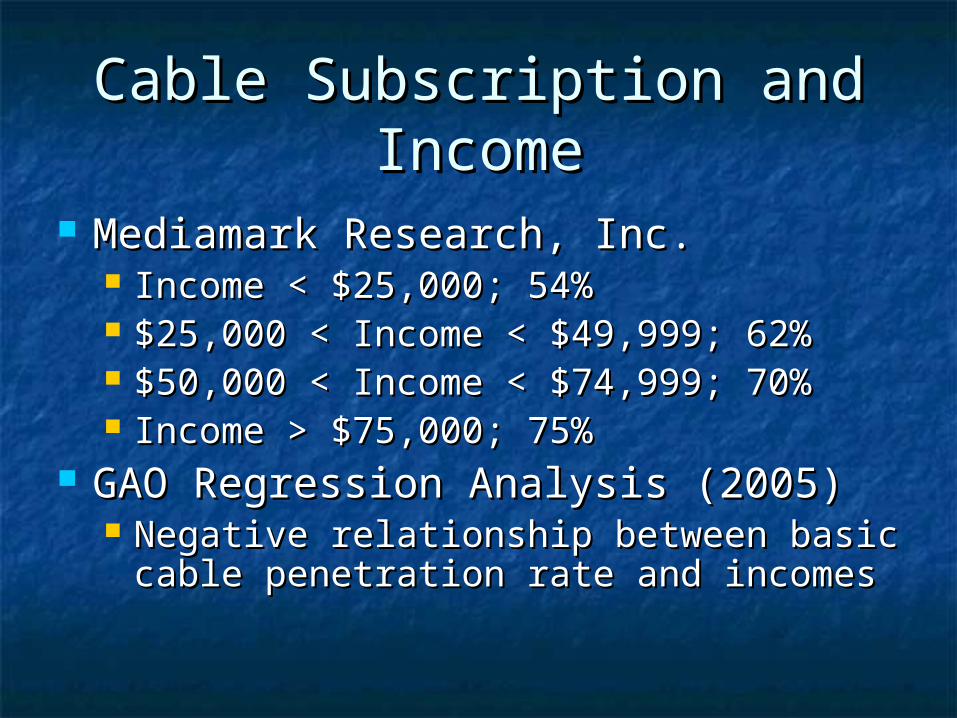
Cable Subscription and Cable Subscription and IncomeIncome
Mediamark Research, Inc. Mediamark Research, Inc. Income < $25,000; 54%Income < $25,000; 54% $25,000 < Income < $49,999; 62%$25,000 < Income < $49,999; 62% $50,000 < Income < $74,999; 70%$50,000 < Income < $74,999; 70% Income > $75,000; 75%Income > $75,000; 75%
GAO Regression Analysis (2005)GAO Regression Analysis (2005) Negative relationship between basic Negative relationship between basic
cable penetration rate and incomescable penetration rate and incomes

Video, Income, DeploymentVideo, Income, Deployment
$
Income (y)
homes ordered by income
r(y): Expected Revenue for home i, which is a function of income y
k: Capital Cost per Home Passed
Phoenix Center Policy Paper No. 23, Figure 1.
y*
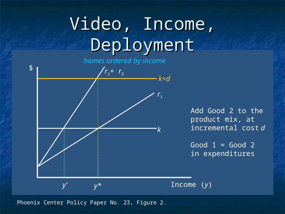
Video, Income, DeploymentVideo, Income, Deployment
$
Income (y)
homes ordered by income
r1
k
Phoenix Center Policy Paper No. 23, Figure 2.
y*y’
r1+ r2k+d
Add Good 2 to the product mix, at incremental cost d
Good 1 = Good 2 in expenditures

Video, Income, DeploymentVideo, Income, Deployment
$
Income (y)
homes ordered by income
r1
k = r3
Phoenix Center Policy Paper No. 23, Figure 3.
y*
r1+ r3
k+d
Add Good 3 to the product mix with Good 1, at incremental cost d
Average of Good 1 = Good 3, but Good 3 has no relationship to income
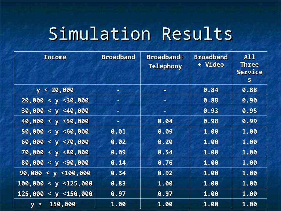
Simulation ResultsSimulation ResultsIncomeIncome BroadbandBroadband Broadband+Broadband+
TelephonyTelephonyBroadbanBroadband + Videod + Video
All All Three Three
ServiceServicess
y < 20,000y < 20,000 - - 0.84 0.88
20,000 < y <30,00020,000 < y <30,000 - - 0.88 0.90
30,000 < y <40,00030,000 < y <40,000 - - 0.93 0.95
40,000 < y <50,00040,000 < y <50,000 - 0.04 0.98 0.99
50,000 < y <60,00050,000 < y <60,000 0.01 0.09 1.00 1.00
60,000 < y <70,00060,000 < y <70,000 0.02 0.20 1.00 1.00
70,000 < y <80,00070,000 < y <80,000 0.09 0.54 1.00 1.00
80,000 < y <90,00080,000 < y <90,000 0.14 0.76 1.00 1.00
90,000 < y <100,00090,000 < y <100,000 0.34 0.92 1.00 1.00
100,000 < y 100,000 < y <125,000<125,000
0.83 1.00 1.00 1.00
125,000 < y 125,000 < y <150,000<150,000
0.97 0.97 1.00 1.00
y > 150,000 y > 150,000 1.00 1.00 1.00 1.00

SummarySummary
We are now faced with a facilities-based We are now faced with a facilities-based only entry method into local markets only entry method into local markets (video, voice, and data)(video, voice, and data)
We must eliminate any unnecessary We must eliminate any unnecessary barriers to facilities-based entry if we are barriers to facilities-based entry if we are to have competitionto have competition Market limitationsMarket limitations Build-out RulesBuild-out Rules Etc.Etc.

SummarySummary
Consider the source of policy proposalsConsider the source of policy proposals Build-out rules are only good for cable Build-out rules are only good for cable
incumbents if entry is deterred; thus, they incumbents if entry is deterred; thus, they are betting on entry deterrenceare betting on entry deterrence
Cross-subsidy is the enemy of Cross-subsidy is the enemy of competition, because competition is competition, because competition is the entry of cross-subsidythe entry of cross-subsidy Social agendas may need to be re-Social agendas may need to be re-
evaluated and refinancedevaluated and refinanced