Comparison of transcription factor binding sites from ChIP-seq experiments

by

Colin Diesh

The University of Colorado, Boulder Department of Computer Science

May, 2013

 

 

The Thesis Committee for Colin Diesh Certifies that this is the approved version of the following thesis (or report):

SUPERVISING COMMITTEE:

Debra Goldberg

Robin Dowell

Andrzej Ehrenfeucht

 

   

 

 

Comparison of transcription factor binding sites from ChIP-seq experiments

by

Colin Diesh

A thesis submitted in partial fulfillment of requirements of the Degree of Bachelor of Science in Computer Science

The University of Colorado, Boulder May, 2013

   

 

 

Comparison of transcription factor binding sites using ChIP-seq experiments

Abstract

Transcription factors play an important role in gene regulation by binding and interacting with DNA. Identifying the DNA-binding activity for transcription factors and other proteins has become an important problem for understanding gene regulation. Chromatin immunoprecipitation combined with high-throughput sequencing (ChIP-seq) has been used to analyze DNA-protein interactions, such as transcription factor binding, experimentally. Unfortunately, the metrics for identifying transcription factor binding sites are not directly comparable across experiments, which makes it difficult to assess the significance of the conserved and differential binding sites. We created software for comparing ChIP-seq experiments using a hypothesis testing approach, and apply our method to reveal differential binding sites among yeast strains.

 

 

Table of Contents Section 1: Introduction Subsection 1.1: Chromatin immunoprecipitation, ChIP-chip, and ChIP-seq Subsection 1.2: Finding transcription factor binding sites Subsection 1.3: Existing algorithms for comparing ChIP-seq data Section 2: Approach Subsection 2.1: Description of dataset Subsection 2.2: Analyzing the parent strains Subsection 2.3: Processing of data Subsection 2.4: Normalizing using scaling by read counts Subsection 2.5: Comparison of replicate experiments Subsection 2.6: Comparison of different strains Subsection 2.7: Normalization using NormDiff Section 3: Testing for differential binding sites Subsection 3.1: Statistical characterization of the ordinary t-test Subsection 3.2: Statistical characterization of the moderated t-test Subsection 3.3: Identifying differential peaks Subsection 3.4: Comparison with other programs Subsubsection 3.4.1: Comparison with DIME Subsubsection 3.4.2: Comparison with MACS Subsection 3.5: Considerations Section 4: Future work Section 5: Conclusions

 

 

1 Introduction The study of eukaryotic genomes has revealed a complex world of proteins that bind to DNA to regulate gene expression. Transcription factors are one type of DNA-binding protein that is important for regulating genes. Most transcription factors tend to bind to specific DNA sequences and influence the expression of nearby genes. Finding these binding sites and profiling the activity of transcription factor binding under different conditions has become important for understanding gene regulation, however, studies have shown that these binding sites can vary significantly between related species, and even between closely related individuals [20, 9]. These types of changes in DNA-binding are studied to reveal clues about how the genome regulatory system works. Chromatin immunoprecipitation is an experimental methodology that is used to profile the binding sites of DNA-binding proteins. Essentially, chromatin immunoprecipitation uses specific antibodies to isolate a particular protein and the DNA it is attached to. The DNA fragments can then be analyzed to show where these binding sites are on the genome. One such method uses chromatin immunoprecipitation combined with high throughput sequencing (ChIP-seq) to sequence the DNA fragments produced from chromatin immunoprecipitation. ChIP-seq produces millions of short DNA sequence reads that are enriched for particular DNA-binding sites. After aligning the short reads to a reference genome, this method can provide a whole-genome view of a particular transcription factor’s binding sites. New computational techniques have been developed to address problems of analyzing high-throughput data. In the area of ChIP-seq in particular, there have been many algorithms for finding transcription factor binding sites, but many of these algorithms are only used to analyze individual experiments, and are not used to compare experiments [17]. While it is important to be able to identify features from individual high-throughput experiments, it has not been clear how the metrics that characterize the binding sites from peak finders can be compared across different experiments. In order to compare results from different ChIP-seq experiments, normalization can be used to account for different experimental variables. Different types of normalizations have been developed to account for variables in ChIP-seq, and one common method for normalizing high-throughput sequencing data is scaling for read depth [19, 20]. Other methods for normalizing have been developed to estimate the background noise to improve scaling factors [3, 7], to use a linear model to scale read depth [12], and to estimate changes in the variance of the data across the genome to reduce bias [20, 19, 6]. These normalization methods are helpful for comparing the results from different ChIP-seq experiments, and also just for comparing a ChIP-seq against a control.

 

 

Another consideration for comparing experiments is the appropriate use of statistical testing. A variety of statistical models have been developed for finding binding sites from individual experiments (see [17]), but there are also some methods that focus on comparing ChIP-seq experiments. The methods that have been used for comparing ChIP-seq experiments include a Bayesian Poisson model to find conserved binding sites [12], negative binomial models to model variance across experiments [11, 4, 6], estimating mixture-model for evaluating differential binding sites [16], using the variance of the read scores across experiments to find variable binding regions [20], and by directly comparing experiments using a dynamic Poisson [19]. Each of these methods have unique approaches that address different concerns, and each is suited to particular applications, but some of these methods have drawbacks such as not being able to incorporate replicate experiments into their analysis [12, 19, 16]. We created software for comparing ChIP-seq experiments using a hypothesis testing approach to reveal differential binding sites among yeast strains. We adopted a statistical framework from the limma package [13] that uses a “moderated t-test”, which was developed for comparing gene expression data for microarrays, to compare ChIP-seq data [13]. This framework has some advantages over other methods for comparing ChIP-seq experiments, including the ability to incorporate replicates. We use the moderated t-test to find significant differential binding sites from ChIP-seq experiments and this approach offers flexible options for data analysis and experimental design.

1.1 Chromatin immunoprecipitation, ChIP-chip, and ChIP-seq

Chromatin immunoprecipitation (ChIP) is an experimental methodology that can be used to find the binding sites of DNA-binding proteins. ChIP uses a special antibody to target a protein of interest, and then the protein and the DNA to which it is bound are precipitated from the mixture. Then, the proteins are unlinked from the DNA, resulting in a DNA library that is enriched for the binding sites of that particular protein. Many different variations of the ChIP protocol have been developed [2] but the main outline of the protocol is shown in Figure 1↓. In order to interpret the DNA fragments from a ChIP experiment, additional steps can be applied. Classical methods for analyzing DNA fragments have used PCR (polymerase chain reaction) and electrophoresis gel, but newer “high-throughput” techniques are now popular which can analyze many different fragments of DNA simultaneously. Different types of high throughput technologies have been developed which, when used with ChIP, can provide a large scale or whole-genome view of DNA-protein interactions [2]. DNA microarrays are one type of high-throughput technology that can analyze the DNA fragments from a ChIP experiment (ChIP-chip). ChIP-chip applications utilize microarrays

 

 

which are covered with short DNA probes that hybridize to the DNA fragments. Microarrays have been developed for yeast to cover the whole genome, but for other genomes such as mouse and human, the microarrays are printed with oligonucleotides from upstream regions of the target genes in order to detect the transcription factors that are the most likely regulators [9]. Using so-called tiled arrays or high-density microarrays increases the resolution that binding sites can be detected. Another method known as ChIP-seq uses high-throughput sequencing to analyze the DNA fragments of a ChIP experiment. High-throughput sequencing creates millions of short DNA reads (20-50bp) which are produced from sequencing the 3’ end of the DNA fragments. A general overview of the ChIP-seq workflow is shown in Figure 1↓. Essentially, the ChIP-seq protocol uses high-throughput sequencing of the ChIP DNA fragments and uses DNA alignment algorithms to map the short reads to the genome. This produces millions of short reads that are enriched for the DNA associated with a particular DNA-binding protein and can be used to find the binding sites. The data is also fairly noisy because ChIP is an enrichment protocol. To estimate the significance of the peaks, control data can be generated by sequencing the DNA without any anti-body targets, which is called input control DNA. There are many problems for analyzing this data and for finding transcription factor binding sites. The main idea is that many of the short read sequences repetitively cover a particular region of the DNA forming peaks where there are binding sites These peak finding algorithms are common for detecting transcription factor binding sites from ChIP-seq data and we discuss them in the next section.

 

 

Figure 1 The ChIP-seq workflow: chromatin immunoprecipitation and aligning sequences. The outline of the ChIP-seq protocol including chromatin immunoprecipitation with sequencing and alignment of DNA (Wikipedia:ChIP-seq).

1.2 Finding transcription factor binding sites

To find transcription factor binding sites, peak finding algorithms are commonly used to find regions of the genome where ChIP-seq read counts exceed a certain threshold. The statistical problem of peak finding is a classic one: peak finders must be discriminative enough to avoid false positives, but they must also be sensitive enough to avoid false negatives. We looked at a popular and open-source software package for peak finding called MACS (Model-based analysis

 

 

of ChIP-seq) to see how potential binding sites are identified from ChIP-seq data [19]. A brief overview of peak finding algorithm that MACS uses is as follows: The first step MACS uses is to build a peak model to estimate the original size of the DNA fragments. This step is important for peak calling because, conceivably, the transcription factor can bind to any location on the DNA fragment, and so using only the short reads to find binding sites might misrepresent their true location. To estimate the size of the original DNA fragments, a peak model is used to estimate the distance between the bi-modal distribution of sense and anti-sense reads (Figure 2↓). Small peaks are found using a naïve peak finder based on fold-changes on each strand, and then the median distance between pairs of peaks is used to represent the DNA fragment length.

Figure 2 Fragment size estimation using the distribution of paired-end reads. Estimating the fragment size can be used to improve peak finding and is often used for identifying transcription factor binding sites [10].

 

 

After building a peak model, MACS uses a “dynamic” Poisson rate parameter to estimate the background distribution of reads for the whole-genome as well as for local regions. The estimation of the background from local regions can help reduce the bias that has been observed in the promoter regions or from other sources of bias [6, 8]. If control data exists, then the Poisson parameters are estimated from the control data, otherwise, the ChIP-seq data itself is used to estimate the background. Since the number of reads might be different between ChIP-seq and control, the lambda parameter is scaled by the ratio between the total number of reads in the ChIP-seq/total number of reads in the control. The size of the scanning window is equal to 2d, where d is the estimated DNA fragment size (default is d = 100bp). Peaks are identified when the number of reads in the scanning window exceeds a certain likelihood, and then nearby windows that exceed the given threshold are merged together to form peaks.

Figure 3 Peak calling using the Poisson distribution with example peak (Left) The probability of observing a large number of reads for a given Poisson parameter lambda is used to find peaks in the ChIP-seq data using programs like MACS (Wikipedia:Poisson distribution). (Right) An example of a peak identified from yeast ChIP-seq data that shows the repetitive coverage of DNA sequences by short paired-end reads (blue and red) [17]. Identifying peaks is important for finding potential transcription factor binding sites, but it can be difficult to compare these results between experiments. For instance, the number of reads in a peak region can depend on non-biological variables such as the ChIP-seq enrichment and the library size. Other metrics such as the false discovery rate (FDR) and p-value also represent confidence in the peaks, but this is explicitly related to the confidence compared with the background, which makes comparisons of data difficult. Performing a more direct comparison of the ChIP-seq data by including normalization and statistical comparisons can give a better assessment of how transcription factor binding sites vary across experiments.

1.3 Existing algorithms for comparing ChIP-seq data

 

 

A variety of methods have been proposed for comparing transcription factor binding sites from different ChIP-seq experiments. For example, by comparing the overlapping and non-overlapping genome regions using the peaks identified from individual ChIP-seq experiments, one can get an idea of the qualitative differences of the binding sites. One can also look at the “target” gene for each peak by annotating the peaks with the nearest genes, and look at the overlapping set of gene IDs [20, 9]. These approaches are useful to get an overall sense of the binding site similarities and differences, but it does not provide a sense of differential quantification. MACS can perform a comparison of ChIP-seq experiments to find differential binding sites in addition to calling peaks on individual experiments. In order to find these differential binding sites, one ChIP-seq experiment is used as a false control data (instead of the typical use of a input DNA as a control), and another ChIP-seq experiment is used to compare against it as usual. Then, differential peaks are found when large peaks in the data are found to exceed the false control. This technique is possible because the background variation of the Poisson, assuming that the background variation is comparable across experiments. This method has some intuitive advantages for finding differential peaks, however, it does not satisfy some problems. One of the problems with the approach that MACS uses is that it does not necessarily incorporate replicate data into its findings. To incorporate replicates into MACS, the reads from the replicate experiments can be pooled simply by concatenating the read files. Pooling replicate experiments will increase the “saturation” and total sequencing depth however it does not give you testing intuition that could be derived for replicate experiments. Alternatively, the overlapping or non-overlapping peaks from replicate experiments could be used to incorporate the high confidence peaks, however this still doesn’t necessarily increase confidence for these peaks since it will also increase the background noise. Replicates have been shown to be important in measuring differential gene expression using microarrays [18], and we considered methods that use similar techniques that would help us compare ChIP-seq data to find differential binding sites. The statistical problem that arises from doing comparisons from high-throughput data is the “small n, large p” problem. This problem exists because typically there are few samples (n) for high throughput data, but a lot of hypothesis tests (p) about which sites are significantly different [18].

2 Approach To tackle the problem of comparing these large high-throughput sequencing datasets for ChIP-seq data we first conducted exploratory analysis and describe the dataset being used (2.1, 2.2). Then we do preprocessing of the data to build a datastructure for comparing ChIP-seq experiments (2.3). Then we performed a simple normalization of our data using scaling by

 

 

median read depth (2.4). We looked for evidence for differential binding sites by looking at the read counts of the overlapping and non-overlapping peaks that are found from different experiments (2.5, 2.6). Finally, we evaluated the NormDiff algorithm [20] for comparing experiments (2.7).

2.1 Description of dataset

We looked at ChIP-seq experiments for two different strains of yeast for a transcription factor Ste12 accessed from Zheng et al. [20]. The two different strains of yeast are called S96, which is isogenic to the reference S288c strain of “baker’s yeast”, and HS959, which is isogenic to the YJM789 strain (a clinical isolate).. The reads from both S96 and HS959 were aligned to the same reference genome, S288c, and these mapped short-read sequences are used by our algorithm. Aligning to the same reference genome makes a reasonable simplifying assumption about the similarity of both genomes. In this work we do not consider the alignment of the YJM789 genome to S288c for comparing the ChIP-seq reads.

2.2 Analyzing the parent strains

Goal: In the original analysis of these genomes, Zheng et al. observed “extensive Ste12 binding variation among individuals” [20]. This variation refers to not only differences between the two parent strains, but also variations in the cross-strains from the parent strains. To show just the differences between the parent strains, Zheng et al. obtained the target genes for the binding sites that are found using MACS by annotating the peaks with the nearest gene ID. We wanted to reproduce these results in order to see if the binding site differences between the parent strains are found from non-overlapping gene IDs from the peak finding results. Methods: We obtained the published set of peaks that are called using MACS that were published by Zheng et al. in the GEO repository. The peak annotations were made using the nearest promoter ID from the nearest gene using annotations from the sacCer3 genome database. Results: We found similar results using the gene annotations of the peak set with the gene set that Zheng et al. published (Table 2↓). There is a similar distribution from the overlapping and non-overlapping gene IDs.

 

 

Genome Annotated target genes

S96 unique 292

Overlap 843/820 non-redundant

HS959 unique 336

Figure 4 Comparison of our annotation of the target genes compared with original published results (Top) Results from peak annotation of the peaks published by Zheng et al. with sacCer3 annotation (Bottom) Original results from Zheng et al. showing the overlap of the gene sets identified from the peaks in S96 and HS959 [20]

2.3 Processing of data

Goal: In order to do our own analysis of the ChIP-seq experiments, we needed to produce data that has a suitable format. After analyzing read counts, the data is in ragged arrays with each chromosome having its own array. We joined the data from each array from all of the ChIP-seq experiments into a single data table to make comparing the data easier. Method: We counted the number of reads that overlap small non-overlapping bins of length n = 10bp for each experiment over the whole genome using MACS [19]. Then we merged the set of read counts from each experiment into a single data table by using an inner-join relationship, matching on genome position. Reads that have zero counts are considered missing data and they are omitted from the data table. Result: The result of joining the experiments together is a large data table with columns that correspond to the chromosome, genome position, and read counts for each experiment. We used approximately 118mb for this table (in memory) for the yeast ChIP-seq experiments, only including the parent strain replicates (genome size 1.2*10^7bp, bin size n = 10bp).

 

 

Caveat: We use an inner-join of the read positions because empty bins are considered missing data, so we simply omit these from processing. Note that if we performed an outer-join instead of an inner-join, then it would include empty bins and they could be filled in with zero reads and it could be included for downstream processing. We omit these because positions with zero mapped reads often indicates a problem with mappability of the genome, and because this causes problems with taking log-ratios of the genes.

2.4 Normalizing using scaling by read counts

Goal: The data from different ChIP-seq experiments have different total library sizes of the number of sequenced reads, and this can influence the results of comparing the experiments. We wanted to normalize the data based on the median read depth so that the “background” distribution that represents the majority of the data would be equalized. Method: We took each column of the data table and calculated the average values of the median of each column’s distribution. Then, the difference between the column’s median and the average value over all columns is used to scale the read depth. Result:

Figure 5 Comparison of the read depth before and after normalizing (Left) The boxplot for the read depth of 2 replicates for S96 versus 2 replicates for HS959 (Right) The boxplot after normalizing for the median read depth across all distributions.

 

 

ChIP-seq data file Total library size (number of reads)

S96ChIP_rep1 2218566

S96ChIP_rep2 1292603

S96input 1335253

HS959ChIP_rep1 1106212

HS959ChIP_rep2 1300837 HS959input 1024275

Table 2 Listing of total number of sequenced reads for ChIP-seq and control data created for each experiment Interpretation: After normalizing, the median values are equalized across all the experiment (Figure 5↑). The normalization has the effect of making the median read depths equal, but note that the median read depth is not necessarily correlated with the total library size. For example HS959rep1 has a greater average read depth (Figure 5↑) but it does not have a larger library size (Table 2↑), which indicates that the enrichment of the ChIP protocol can vary across experiments causing different signal to noise ratios. Caveats: Our method of equalizing the distributions based on median read depth might be seen as more aggressive than some other methods such as just scaling by the total library size, however, it is less aggressive than a full quantile normalization. Additionally, more sophisticated normalizations have been developed that can estimate the background [3, 7]. However, scaling by median read depth is not too uncommon, and in fact, was also used by Zheng et al. [20] for comparing ChIP-seq and control data.

2.5 Comparison of replicate experiments

Goal: For each of the strains of yeast that Zheng et al. used, at least two biological replicate experiments were performed using ChIP-seq. We specifically wanted to see if we could find any differences between the overlapping or non-overlapping peaks that were identified using MACS. Methods: We used ChIP-seq read counts from bins with matching genome positions in two S96 replicates and compared the counts from the bins that are in the overlapping peaks and non-overlapping

 

 

peaks. Note that bins with zero reads are excluded, but even bins with low read counts can fall within peak regions. Results: We found that the read counts from the replicates have high correlation (ρ > 0.9). With regard to the peak read counts, the non-overlapping peaks have smaller read counts compared with the read counts of the overlapping peaks. However, notably, even for the non-overlapping peaks, there do not appear to be large differences between the read counts (Figure 6↓). Interpretation: From our analysis of the peaks from these replicates, even the non-overlapping peaks seem to have similar read counts based on our figure, which suggests that simply using the non-overlapping peaks to represent differences might be misrepresenting the data. Note that the reads from the replicate 1 appear higher in some of the peaks in replicate 2 (Figure 6↓), and vice versa, because after normalizing by median read depth S96rep2 gets an average increase in read counts (see Figure 5↓).

Figure 6 Comparison of S96 replicates showing the distribution of read counts in the overlapping peaks and non-overlapping peaks. (Left) The replicates have a high correlation (>0.9) across the whole genome and peaks that are non-overlapping are clustered about y=x showing that they are not very different. (Right) The log2-transform does not show large differences either (lines indicate fold-change>4).

2.6 Comparison of different strains

Goal:

 

 

We wanted to compare the different strains of yeast to see if we could find differential binding sites from overlapping and non-overlapping peaks that are identified using MACS. This comparison might show more interesting features because, while the replicate experiments are biological/conditional copies of each other, finding differences in the binding sites from different strains might show some functional or regulatory change in their genomes. Methods: Similar to our analysis of the replicates, we use the read counts from the peaks called by MACS from one replicate in each strain of S96 and HS959, and look at how the read counts from overlapping and non-overlapping peaks compare. Note that the ChIP-seq data from both strains is aligned to the same reference genome, so we use the same genome coordinates when comparing the experiments. Results: By comparing the raw read counts, there appear to be clear differences between the peaks that are unique to each dataset (Figure 7↓). Looking at the log-transform shows large fold-change differences too. The read counts from the non-overlapping peaks are significantly differentiated from the overlapping peaks, albeit with smaller read counts. Interpretation: Our plot shows evidence for differential binding sites simply from looking at the non-overlapping peaks. The read counts from the non-overlapping peaks are significantly differentiated from the overlapping peaks, albeit with smaller read counts. The significance of the differential binding sites can’t be assessed using this figure, but it provides a qualitative overview of the differences between the binding sites from each strain.

 

 

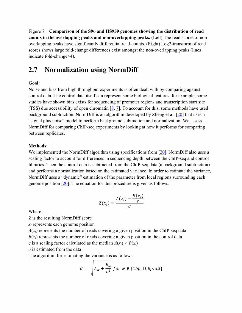
Figure 7 Comparison of the S96 and HS959 genomes showing the distribution of read counts in the overlapping peaks and non-overlapping peaks. (Left) The read scores of non-overlapping peaks have significantly differential read-counts. (Right) Log2-transform of read scores shows large fold-change differences exist amongst the non-overlapping peaks (lines indicate fold-change>4).

2.7 Normalization using NormDiff

Goal: Noise and bias from high throughput experiments is often dealt with by comparing against control data. The control data itself can represent some biological features, for example, some studies have shown bias exists for sequencing of promoter regions and transcription start site (TSS) due accessibility of open chromatin [8, 7]. To account for this, some methods have used background subtraction. NormDiff is an algorithm developed by Zheng et al. [20] that uses a “signal plus noise” model to perform background subtraction and normalization. We assess NormDiff for comparing ChIP-seq experiments by looking at how it performs for comparing between replicates. Methods: We implemented the NormDiff algorithm using specifications from [20]. NormDiff also uses a scaling factor to account for differences in sequencing depth between the ChIP-seq and control libraries. Then the control data is subtracted from the ChIP-seq data (a background subtraction) and performs a normalization based on the estimated variance. In order to estimate the variance, NormDiff uses a “dynamic” estimation of the parameter from local regions surrounding each genome position [20]. The equation for this procedure is given as follows:

𝑍 𝑥! =𝐴 𝑥! − 𝐵 𝑥!

𝑐𝜎

Where- Z is the resulting NormDiff score xi represents each genome position A(xi) represents the number of reads covering a given position in the ChIP-seq data B(xi) represents the number of reads covering a given position in the control data c is a scaling factor calculated as the median A(xi) ⁄ B(xi) σ is estimated from the data The algorithm for estimating the variance is as follows

𝜎 =   𝐴! +𝐵!𝑐!  𝑓𝑜𝑟  𝑤 ∈ {1𝑏𝑝, 10𝑏𝑝,𝑎𝑙𝑙}

 

 

We implemented the NormDiff algorithm using specifications from Zheng et al. [20] using the R programming language. We assessed the fit of NormDiff to compare replicate ChIP-seq experiments from the S96 strain of yeast. Additionally, we looked at how NormDiff compares to other types of normalization such as background subtraction without normalization and a modified NormDiff with only global variance estimation. Results: The result of these comparisons is that NormDiff with local variance estimation has better normalizing properties than the global variance estimation, or a comparison of reads without normalization, and it results in a less biased normalization than the other methods (Figure 8↓). Interpretation: The NormDiff algorithm is well-suited to normalizing the “binding signal” and removes bias caused by differences in read depth and other variables. The result of the normalization can be made clear by observing that the total number of reads from replicate 1 is almost twice the number of reads from replicate 2 (see Table 2↑). Even so, NormDiff effectively normalizes both experiments which can be seen by comparing the differences between all positions (Figure 8↓).and observing that the least squares best fit line has slope close to zero (slope=0.02). NormDiff does not perform any between-experiment normalizations, but by estimating the binding signal and by performing a background subtraction, it tries to make the ChIP-seq experiments comparable. Caveat: One problem with NormDiff is that it has increased noise due to the additive effect of the variance in the background subtraction. While it controls the bias of the signal, it also increases the variance, which is known as the Bias-Variance trade-off. Since the quantitative trait should accurately measure the variance it’s possible that the background subtraction techniques introduce too much noise.

 

 

Figure 8 The sum versus the difference of S96 replicates read counts using different normalization techniques and including the line of best fit (a) Using background subtraction with scaling for read depth (b) NormDiff with variance parameter estimated from all points (c) NormDiff with local variance estimation parameter.

3 Testing for differential binding sites

3.1 Statistical characterization of the ordinary t-test

Goal: In order to find differential binding sites from ChIP-seq data, we wanted to find where the difference between the read counts was statistically significant. We wanted to apply a two-sample t-test to find the differences between experiments, however we found problems from the basic methods of the t-test and we sought to characterize these drawbacks. Methods: One method for the statistical comparisons of two groups is Student’s t-test [18], which finds the significance of the mean difference between groups. Student’s t-test has the form

 

 

𝑡 =𝑋! − 𝑋!

𝑠! 1𝑁!+ 1𝑁!

where- Xi is the sample mean s is the pooled sample variance Ni is the sample size Two main features of Student’s t-test should be noted. The first is that the difference between the groups is estimated using the mean difference of the samples. In our application, the differences correspond to the log ratio of the read counts, because log(R/G)=log(R)-log(G). The second is that the t-test assumes that read counts are approximately normally distributed. Results: We looked at the distribution of the log-ratios from each group over the whole genome and found that they follow tend to follow a normal distribution (Figure 9↓). The plots have comparison between genomes has heavy tails, while the comparison of two replicates shows a higher than expected distribution which might come from the fact that no very large differences exist to even out the bell curve. Interpretation: Even though these distributions log-ratios across the whole genome appear normal, this is a heuristic view of the desired distribution. This is because we are not necessarily interested in comparing different positions in the genome, but rather that the distribution of the read counts at a particular genome position across experiments. Caveats: Overall, the ordinary Student’s t-test is not well suited for our data for several reasons. One problem is that we have a small number of samples, so it is difficult to estimate the variance from the binned read counts at a particular genome position. Another problem is that the variance of the read counts is small for most of the genome because and this low variability causes problems.

 

 

Figure 9 The distribution of the log-ratios for comparing different ChIP-seq experiments is approximately normal. The quantiles of the log-ratios of binned read counts of (left) S96rep1/HS959rep1 and (right) S96rep1/S96rep2 versus the expected quantiles of the standard Normal distribution (red).

3.2 Statistical characterization of the moderated t-test

Goal: While the classical t-test methods were insufficient for comparing ChIP-seq data, we noted that some algorithms that are used for comparing differential gene expression microarrays have used different types of t-tests that address the shortcomings of the classical t-test for high-throughput data [5, 14]. We sought to apply methods from the limma package to improve finding differential binding sites from ChIP-seq data [13]. Methods: The limma package uses a linear model that analyzes the errors vs the log ratios of all the data in a high throughput experiment and then performs a moderated t-test based on the estimation of the variances [14]. We used the log ratios of pairs of each replicate as input to the algorithm, e.g. the log-base-two of the normalized read scores of S96rep1/HS959rep1 and S96rep2/HS959rep2. The linear model for each position that is calculated as

𝐸 𝑦! = 𝑋𝛼! Where- yg is the set of inputted log ratios X is the design matrix αg is the set of log-ratios to estimate from the linear model In our two-sample comparison, each set of log-ratios is treated as a replicate, so the design matrix is simply a vector of ones with length n=number of pairs of replicates. Then the

 

 

coefficients of αg are used to estimate the expected log ratios E(yg). Then the errors of this linear model are used to estimate the standard deviations for the t-test. The moderated t-test uses the mean standard deviation across all the entire dataset s0 and adds it to the estimated standard deviation at each position. The moderated t-test “has the same interpretation as an ordinary t-statistic except that the standard errors have been moderated across genes, i.e., shrunk towards a common value, using a simple Bayesian model.” [14]. Therefore, the values with small variance will be scaled up from 0 to receive larger variance. Results: The moderated t-test results have a good model fit (Figure 10↓) and it prevents many of the errors that were previously encountered with the ordinary t-test. We looked at a histogram of the FDR adjusted p-values and found many significant differential binding sites with (P<0.05). Interpretation: The moderated t-test helps to correct small variance in the background region by using the mean standard deviation s0 to the variance pool that represents a common standard deviation for the whole dataset. This addresses the issue of small sample size by using distribution of the variance across the entire genome to get a better estimate of the variance of a particular genome position that is compared with the t-test.

Figure 10 Statistical distributions of moderated t-tests, and the selection of the most highly significant differential binding sites. (left) The distribution of the moderated t-tests follows the expected quantiles of the t-distribution (right) The distribution of the moderated t-tests follows the expected quantiles of the t-distribution (right) FDR adjusted p-values calculated from limma showing many differential binding sites (P<0.05).

3.3 Identifying differential peaks

 

 

Goal: After performing statistical tests, we wanted to inspect the results of our hypothesis testing to identify significant differential binding sites and merge nearby bins with differential read counts bins into differential peaks Methods: We selected an arbitrary number of significantly differential read count bins that are reported by limma. Then nearby bins that are less than 20bp apart from each other that are also significantly differential are merged together to form differential peaks. Other algorithms have used more sophisticated merging methods for combining genome regions by including moving average or hidden Markov models [5]. We do not take this approach and simply combine the nearby read count bins. Results: We selected significant differential peaks by selecting the most significant read counts according to the log-odds ratios given by the empirical Bayes functions of limma from the moderated t-test (Figure 12↓). Then we highlighted the selected positions in the strain vs strain comparison plot to show that the t-test finds significantly differential read counts. After merging the nearby bins from our selection, we obtained 158 unique differential peaks with FDR adjusted P-value <0.01. We inspected the signal tracks of the differential peaks by plotting the number of reads that overlap each genome position (Figure 12↓). Interpretation: The sites that are highlighted in the strain vs strain comparison plot from the differential binding sites that we found correspond with intuition about which sites are differential . Many of the differential binding sites are merged with nearby neighbors to produce differential peaks (Figure 11↓).

 

 

Figure 11 Selecting differential read count bins and merging nearby bins to form differential peaks (left) Selection of an arbitrary number of the most significant differential binding sites from the moderated t-test. (right) The differential read counts from the moderated t-test in a strain vs strain comparison

Figure 12 The differential read counts from the moderated t-test correspond with highly differential peaks (Left) Signal track for a differential peak identified using our algorithm (P<0.0001, log fold-change 4.13) (Right) A broad differential peak identified using limma.

. Figure 13 Comparison of the number of merged peaks versus the number sites inputted to the merge algorithm. (Left) The merged peaks accumulate faster than the number of sites that are inputted (Right) The ratio between the input to the output of the merge algorithm is small and decreases as the p-value threshold adds more inputs to the algorithm.

3.4 Comparison with other programs

Goal: We sought to compare the set of differential peaks that we identified with other programs including DIME and MACS. DIME uses an expectation maximization (EM) for a mixture model to identify a differential component of a mixture model of distributions [15]. The MACS

 

 

approach for finding differential binding sites uses estimation of the background from a false control (a ChIP-seq experiment instead of input controls) [19].

3.4.1 Comparison with DIME  

Methods: We used the same median scale normalized log-ratio inputs to DIME to calculate the most significant differences. DIME calculates the best fit from several types of mixture models including a normal plus uniform distribution (NUDGE), K-normal plus uniform (iNUDGE) or GNG (gamma-normal-gamma). We ran the EM algorithm for 50 iterations and used the best model for downstream processing. Then we merged nearby read count bins to form differential peaks, Results: In our trial, with 50 iterations of the EM algorithm, DIME uses is not able to find a differential component of the mixture model. Still, the results of the model can still be useful. The claim is made is that “applicability of DIME is greatly extended beyond uniform or exponential since any distribution can be well approximated by a mixture of normals” [15]. DIME classified 20116 read count bins as differential, and after merging nearby read count bins, we identified 4280 differential binding sites (P<0.01). Interpretation: We use the iNUDGE model from DIME with K=2 normal components which shows a good model fit and use default sigma thresholds for identifying differential binding from the normal components. The differential components that are identified from the strain vs strain comparison plot are intuitively what we expect as differential. Additionally, we found some good differential peaks with reasonable confidence. One binding site we found with DIME shows a binding site that appears to have moved between one genome position to the other (Figure 16↓), a rather unique occurrence. Caveats: We were able to identify some differential sites using DIME, however there were some problems. There are some problems that S96rep2 and HS959rep2 nearly overlap, however, we only comparing log-ratios of S96rep1 and HS959rep1 in our analysis.Another problem is that the p-values we calculated with DIME appear to be blocky (Figure 15↓), making it hard to perform a threshold by p-value.

 

 

Figure 14 Differential binding sites identified by DIME using the iNUDGE model for the S96 vs HS959 read scores. (Left) The strain vs strain comparison plot shows many differential binding sites (Right) QQ-plot of the iNUDGE model vs log-ratios of S96rep1/HS959rep1

Figure 15 The p-values from DIME calculated show a blocky distribution (Left) Histogram of p-values calculated from iNUDGE algorithm (Right) The number of merged peaks grows differential binding sites.

Figure 16 ChIP-seq signal tracks for several differential binding sites identified using DIME (Left) A well characterized differential peak identified by DIME where the position

 

 

appears to have moved between S96 and HS959 (P=0.002). (Right) A differential binding site identified by DIME that is probably actually conserved.

3.4.2 Comparison with MACS  

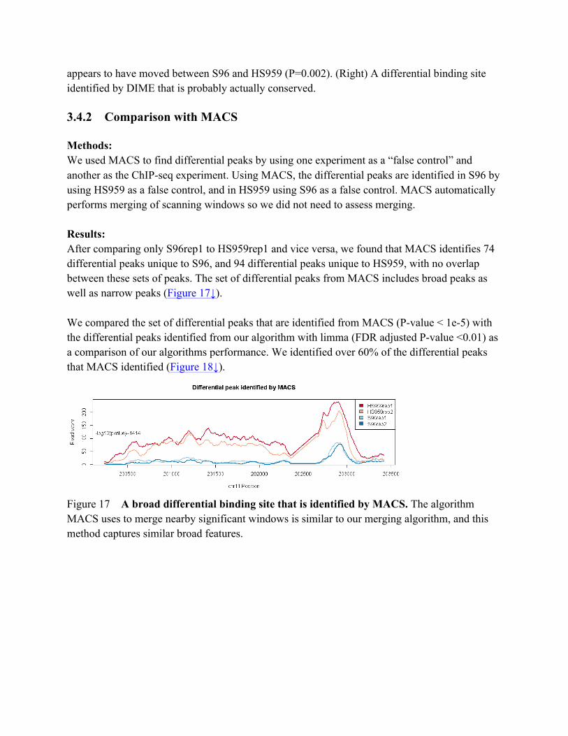
Methods: We used MACS to find differential peaks by using one experiment as a “false control” and another as the ChIP-seq experiment. Using MACS, the differential peaks are identified in S96 by using HS959 as a false control, and in HS959 using S96 as a false control. MACS automatically performs merging of scanning windows so we did not need to assess merging. Results: After comparing only S96rep1 to HS959rep1 and vice versa, we found that MACS identifies 74 differential peaks unique to S96, and 94 differential peaks unique to HS959, with no overlap between these sets of peaks. The set of differential peaks from MACS includes broad peaks as well as narrow peaks (Figure 17↓). We compared the set of differential peaks that are identified from MACS (P-value < 1e-5) with the differential peaks identified from our algorithm with limma (FDR adjusted P-value <0.01) as a comparison of our algorithms performance. We identified over 60% of the differential peaks that MACS identified (Figure 18↓).

Figure 17 A broad differential binding site that is identified by MACS. The algorithm MACS uses to merge nearby significant windows is similar to our merging algorithm, and this method captures similar broad features.

 

 

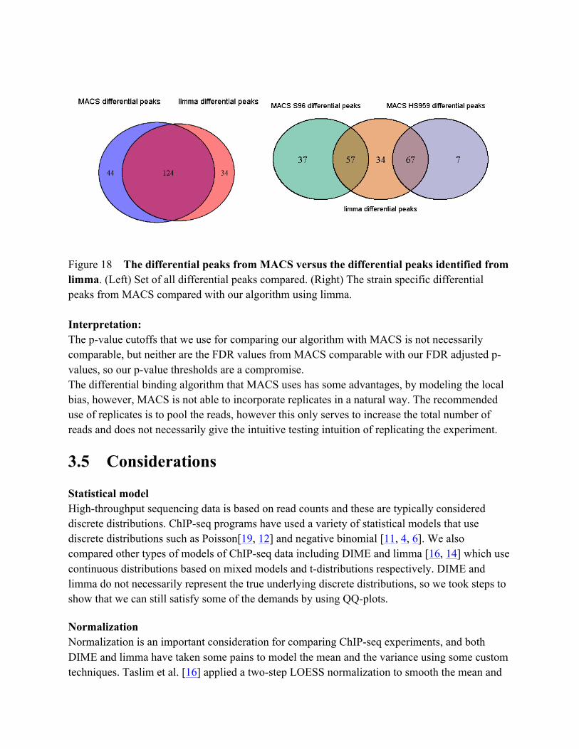
Figure 18 The differential peaks from MACS versus the differential peaks identified from limma. (Left) Set of all differential peaks compared. (Right) The strain specific differential peaks from MACS compared with our algorithm using limma. Interpretation: The p-value cutoffs that we use for comparing our algorithm with MACS is not necessarily comparable, but neither are the FDR values from MACS comparable with our FDR adjusted p-values, so our p-value thresholds are a compromise. The differential binding algorithm that MACS uses has some advantages, by modeling the local bias, however, MACS is not able to incorporate replicates in a natural way. The recommended use of replicates is to pool the reads, however this only serves to increase the total number of reads and does not necessarily give the intuitive testing intuition of replicating the experiment.

3.5 Considerations

Statistical model  High-throughput sequencing data is based on read counts and these are typically considered discrete distributions. ChIP-seq programs have used a variety of statistical models that use discrete distributions such as Poisson[19, 12] and negative binomial [11, 4, 6]. We also compared other types of models of ChIP-seq data including DIME and limma [16, 14] which use continuous distributions based on mixed models and t-distributions respectively. DIME and limma do not necessarily represent the true underlying discrete distributions, so we took steps to show that we can still satisfy some of the demands by using QQ-plots.

Normalization Normalization is an important consideration for comparing ChIP-seq experiments, and both DIME and limma have taken some pains to model the mean and the variance using some custom techniques. Taslim et al. [16] applied a two-step LOESS normalization to smooth the mean and

 

 

the variance separately for comparing ChIP-seq data using DIME. Limma also has a method called voom: mean-variance modelling at the observational level, that uses a LOESS curve to give weights for limma’s linear models. We did not employ these methods of normalization in favor of more simple normalization, scaling median read depth, but there is evidence that these are important for comparing across experiments.

4 Future work Comparisons of ChIP-seq would be improved by better characterizing the variance of the binding sites across experiments. In our approach, we assume a normal distribution in order to apply a t-test, and while we showed a good fit, other distributions that represent the underlying discrete data can be used. One approach that MACS and others have used is to model the local variations of the ChIP-seq data across the genome. This method might be more effective than a whole-genome estimation of variance that limma uses. Others have shown that the Poisson is not as effective at modeling the overdispersion of the variance across experiments, and call for the use of a alternative statistical models [11, 4, 6]. Properly normalizing and characterizing the binding signals from the noisy background would also improve the comparison of ChIP-seq data and help understand the genetic causes of variations in transcription factor binding. Zheng et al. [20] revealed local cis-factors and long-range trans-factors associated with variations in transcription factor binding by using NormDiff to quantify binding. NormDiff uses scaling by median read depth, but better normalization that is used to estimate the background noise separately from the read depth has been shown to be an effective for ChIP-seq data analysis. Applying these methods might help characterize the transcription factor binding sites from the noisy binding signals and reduce the need for background subtraction. Finding the relationship between the binding site changes and gene expression changes can reveal the underlying regulatory patterns for gene expression. Modeling the binding signals more accurately and analyzing the biological variations would be valuable for these types of comparisons. Zheng et al. (2010) compared binding with gene expression to show that the binding sites are highly correlated with gene expression in general (Figure 19↓). We did a comparison of the differential binding with differential gene expression to demonstrate that differential binding is correlated with differential gene expression. We obtained gene expression data for S96 and HS959 using the GEOQuery and GEO2R interface [1]. We used the set of differential binding sites that we identified and compared the log ratios of the differential binding sites with the log ratios of the nearest target gene. This analysis showed that changes to the binding sites influence the expression of the nearby genes.

 

 

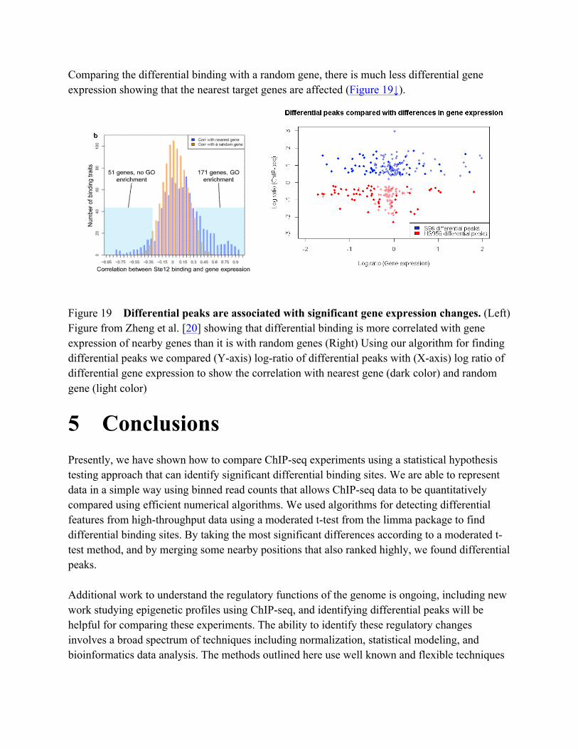
Comparing the differential binding with a random gene, there is much less differential gene expression showing that the nearest target genes are affected (Figure 19↓).

Figure 19 Differential peaks are associated with significant gene expression changes. (Left) Figure from Zheng et al. [20] showing that differential binding is more correlated with gene expression of nearby genes than it is with random genes (Right) Using our algorithm for finding differential peaks we compared (Y-axis) log-ratio of differential peaks with (X-axis) log ratio of differential gene expression to show the correlation with nearest gene (dark color) and random gene (light color)

5 Conclusions Presently, we have shown how to compare ChIP-seq experiments using a statistical hypothesis testing approach that can identify significant differential binding sites. We are able to represent data in a simple way using binned read counts that allows ChIP-seq data to be quantitatively compared using efficient numerical algorithms. We used algorithms for detecting differential features from high-throughput data using a moderated t-test from the limma package to find differential binding sites. By taking the most significant differences according to a moderated t-test method, and by merging some nearby positions that also ranked highly, we found differential peaks. Additional work to understand the regulatory functions of the genome is ongoing, including new work studying epigenetic profiles using ChIP-seq, and identifying differential peaks will be helpful for comparing these experiments. The ability to identify these regulatory changes involves a broad spectrum of techniques including normalization, statistical modeling, and bioinformatics data analysis. The methods outlined here use well known and flexible techniques

 

 

for identifying differential features from high-throughput data and provides a flexible platform for analyzing different types of experiments.

 

 

References [1] T. Barrett, S. E. Wilhite, P. Ledoux, C. Evangelista, I. F. Kim, M. Tomashevsky, K. A. Marshall, K. H. Phillippy, P. M. Sherman, M. Holko, A. Yefanov, H. Lee, N. Zhang, C. L. Robertson, N. Serova, S. Davis, A. Soboleva. NCBI GEO: archive for functional genomics data sets—update. Nucleic Acids Research, 41(D1):D991—D995, 2012. URL http://nar.oxfordjournals.org/content/41/D1/D991.full.

[2] Philippe Collas. Chromatin Immunoprecipitation Assays: Methods and Protocols. Humana Press, aug 2009.

[3] Aaron Diaz, Kiyoub Park, Daniel A. Lim, Jun S. Song. Normalization, bias correction, and peak calling for ChIP-seq. Statistical Applications in Genetics and Molecular Biology, 11(3), 2012. URL http://www.ncbi.nlm.nih.gov/pmc/articles/PMC3342857/. PMID: 22499706 PMCID: PMC3342857.

[4] Hongkai Ji, Hui Jiang, Wenxiu Ma, David S. Johnson, Richard M. Myers, Wing H. Wong. An integrated software system for analyzing ChIP-chip and ChIP-seq data. Nature Biotechnology, 26(11):1293—1300, 2008. URL http://www.nature.com/nbt/journal/v26/n11/abs/nbt.1505.html.

[5] Hongkai Ji, Wing Hung Wong. TileMap: create chromosomal map of tiling array hybridizations. Bioinformatics (Oxford, England), 21(18):3629—3636, 2005. PMID: 16046496.

[6] Pei Fen Kuan, Dongjun Chung, Guangjin Pan, James A. Thomson, Ron Stewart, Sunduz Keles. A Statistical Framework for the Analysis of ChIP-Seq Data. Journal of the American Statistical Association, 106(495):891—903, 2011. URL http://www.tandfonline.com/doi/abs/10.1198/jasa.2011.ap09706.

[7] Kun Liang, Sunduz Keles. Normalization of ChIP-seq data with control. BMC Bioinformatics, 13(1):199, 2012. URL http://www.biomedcentral.com/1471-2105/13/199/abstract. PMID: 22883957.

[8] David A Nix, Samir J Courdy, Kenneth M Boucher. Empirical methods for controlling false positives and estimating confidence in ChIP-Seq peaks. BMC bioinformatics, 9:523, 2008. PMID: 19061503.

[9] Duncan T Odom, Robin D Dowell, Elizabeth S Jacobsen, William Gordon, Timothy W Danford, Kenzie D MacIsaac, P Alexander Rolfe, Caitlin M Conboy, David K Gifford, Ernest Fraenkel. Tissue-specific transcriptional regulation has diverged significantly between human

 

 

and mouse. Nature genetics, 39(6):730—732, 2007. URL http://www.ncbi.nlm.nih.gov/pubmed/17529977. PMID: 17529977.

[10] Peter J. Park. ChIP-seq: advantages and challenges of a maturing technology. Nat Rev Genet, 10(10):669—680, 2009. URL http://dx.doi.org/10.1038/nrg2641.

[11] Mark D Robinson, Davis J McCarthy, Gordon K Smyth. edgeR: a Bioconductor package for differential expression analysis of digital gene expression data. Bioinformatics (Oxford, England), 26(1):139—140, 2010. PMID: 19910308.

[12] Zhen Shao, Yijing Zhang, Guo-Cheng Yuan, Stuart H. Orkin, David J. Waxman. MAnorm: a robust model for quantitative comparison of ChIP-Seq data sets. Genome Biology, 13(3):R16, 2012. URL http://genomebiology.com/2012/13/3/R16/abstract.

[13] Gordon K. Smyth. Limma: linear models for microarray data. In Bioinformatics and Computational Biology Solutions Using R and Bioconductor (Gentleman, R. and Carey, V. and Dudoit, S. and Irizarry, R. and Huber, W., ed.). Springer, 2005.

[14] Gordon K Smyth. Linear models and empirical bayes methods for assessing differential expression in microarray experiments. Statistical applications in genetics and molecular biology, 3:Article3, 2004. PMID: 16646809.

[15] Cenny Taslim, Tim Huang, Shili Lin. DIME: R-package for identifying differential ChIP-seq based on an ensemble of mixture models. Bioinformatics, 27(11):1569—1570, 2011. URL http://bioinformatics.oxfordjournals.org/content/27/11/1569. PMID: 21471015.

[16] Cenny Taslim, Jiejun Wu, Pearlly Yan, Greg Singer, Jeffrey Parvin, Tim Huang, Shili Lin, Kun Huang. Comparative study on ChIP-seq data: normalization and binding pattern characterization. Bioinformatics, 25(18):2334—2340, 2009. URL http://bioinformatics.oxfordjournals.org/content/25/18/2334.

[17] Elizabeth G. Wilbanks, Marc T. Facciotti. Evaluation of Algorithm Performance in ChIP-Seq Peak Detection. PLoS ONE, 5(7):e11471, 2010. URL http://dx.doi.org/10.1371/journal.pone.0011471.

[18] Ernst Wit. Statistics for Microarrays: Design, Analysis and Inference. John Wiley & Sons, jul 2004.

[19] Yong Zhang, Tao Liu, Clifford A. Meyer, Jérôme Eeckhoute, David S. Johnson, Bradley E. Bernstein, Chad Nusbaum, Richard M. Myers, Myles Brown, Wei Li, X. Shirley Liu. Model-based Analysis of ChIP-Seq (MACS). Genome Biology, 9(9):R137, 2008. URL http://genomebiology.com/2008/9/9/R137/abstract.

 

 

[20] Wei Zheng, Hongyu Zhao, Eugenio Mancera, Lars M. Steinmetz, Michael Snyder. Genetic analysis of variation in transcription factor binding in yeast. Nature, 464(7292):1187—1191, 2010. URL http://www.nature.com/nature/journal/v464/n7292/full/nature08934.html.