Comparison of the discrete singular convolution algorithm ...yzhou/papers/ZhouY2001a.pdf · for...

Computer Physics Communications 143 (2002) 113–135www.elsevier.com/locate/cpc

Comparison of the discrete singular convolution algorithm andthe Fourier pseudospectral method for solving

partial differential equations

S.Y. Yang, Y.C. Zhou, G.W. Wei∗Department of Computational Science, National University of Singapore, 117543 Singapore

Received 28 May 2001; received in revised form 10 September 2001

Abstract

This paper explores the utility, tests the accuracy and examines the limitation of the discrete singular convolution (DSC)algorithm for solving partial differential equations (PDEs). The standard Fourier pseudospectral (FPS) method is alsoimplemented for a detailed comparison so that the performance of the DSC algorithm can be better evaluated. Three two-dimensional PDEs of different nature, the heat equation, the wave equation and the Navier–Stokes equation, are employedto make our assessment. Either the fourth-order Runge–Kutta or the Crank–Nicolson scheme is employed for the temporaldiscretization. The DSC algorithm is projected into the Fourier domain for analyzing its numerical resolution. It is demonstratedthat the accuracy of the DSC algorithm is controllable. Comprehensive comparisons are given based on a variety of timeincrement, grid spacing, wavenumber, and Reynolds number. It is found that the DSC algorithm is an accurate, stable androbust approach for solving these PDEs. 2002 Elsevier Science B.V. All rights reserved.

1. Introduction

There has been an ongoing interest in computational methodology in the past few decades, due to theavailability of inexpensive high-performance computers, which has given tremendous impetus to scientific andengineering computing. Most effort has been focused on developing either global methods [1–7] or local methods[8–17] for solving a variety of partial differential equations (PDEs). There has been much debate among thenumerical computation communities over the advantages and disadvantages of various numerical methods overthe past few decades. In general, the local methods, such as methods of finite differences, finite volumes andfinite elements, are highly localized in the spatial domain, yet delocalized in their spectral domain. In contrast,global methods, such as the Fourier spectral method, are highly localized in their spectral representations anddelocalized in the spatial domain. As a consequence, global methods appear to be more accurate than localmethods. The main advantage of local methods is their flexibility for satisfying special boundary conditionsand for treating complex geometries. For example, methods of finite elements are the dominant approach in

* Corresponding author.E-mail address:[email protected] (G.W. Wei).

0010-4655/02/$ – see front matter 2002 Elsevier Science B.V. All rights reserved.PII: S0010-4655(01)00427-1

114 S.Y. Yang et al. / Computer Physics Communications 143 (2002) 113–135

structural analysis in association with unstructured grids. Finite volume methods are commonly used in fluidflow simulations. Finite difference methods are the major approach for electromagnetic wave propagations.Nevertheless, spectral methods have had tremendous success in several areas, where a high computational accuracyis of particular importance while the geometry of the underlying problem is relatively simple. Typical examplesof these areas include weather prediction, nonlinear waves, simulation of turbulence and seismic modeling.It is desirable to have methods which combine the accuracy of global methods and the flexibility of localmethods.

Discrete singular convolution (DSC) algorithm [18–20] has been proposed as a potential numerical approachfor numerically handling singular integrations. In particular, it has emerged as an intriguing alternative in manysituations—and as a superior one in a few cases for solving partial differential equations. The DSC algorithmhas been applied to a number of scientific and engineering problems, including eigenvalue problems of bothquantum [21] and classical [22] origins, analysis of stochastic process [18,19], simulation of fluid flow in simple[23,24] and complex [25] geometries, and nanoscale pattern formation in a circular domain [26]. It facilitated asynchronization scheme for shock capturing [27] and was utilized to integrate the sine-Gordon equation with initialvalues being close to the homoclinic orbit for which numerically induced chaos can easily occur [28]. In structuralanalysis, the DSC algorithm is the only available numerical method for solving a class of pressing structural designproblems which require the prediction of high-frequency vibration levels [22,29–32]. The underlying mathematicalstructure of the DSC approach is the theory of distributions [33] and the theory of wavelet analysis [20,34]. Oneof the distributions used in the aforementioned applications is the Dirac delta function which is a generalizedfunction following from the fact that it is integrable inside a particular interval but it does not have a valuein the interval. Dirac was the first person who explicitly discussed the properties ofδ in his classic text onquantum mechanics, thusδ is often called Dirac delta function. The general orthogonal series analysis of thedelta distribution was studied by Walter [35], who discussed the numerical use of delta sequences as probabilitydensity estimators.

The connection of various numerical methods has always been a topic of great concern. The relation betweenthe Galerkin algorithm and the Ritz variational principle was studied [36]. The reduction from a global Galerkinmethod to a global collocation method was made [5]. A unified view of finite difference and spectral collocationwas given [6]. The connection of the finite-element, finite-difference and finite-volume methods is now wellunderstood [37]. Recently, it was demonstrated that methods of global, local, Galerkin method, collocation andfinite difference can be derived from a single starting point in the framework of the DSC algorithm [19].

The purpose of this paper is to make a detailed comparison of the performance between the DSC algorithm andthe Fourier pseudospectral (FPS) method aiming at a better understanding of both approaches. This is illustratedby applying both approaches to three two-dimensional (2D) PDEs: the heat equation, the wave equation and theNavier–Stokes equation. These problems are selected because they differ in nature. Moreover, these problems arechosen in favor of the FPS method, which solves problems with periodic boundary conditions. Since the DSCalgorithm is a local approach in general, there is no doubt that it is much more flexible than the FPS method indealing with complex geometry and boundary conditions. Computational accuracy is of particular concern in thiswork. Overall, the DSC method is found to be competitive with, or even better than the spectral method on manycomputational aspects.

This paper is organized as follows. A brief description of both the DSC algorithm and FPS method is givenin Section 2. The treatment of spatial discretizations by using both the DSC and the FPS methods is presented.These methods are further discussed in connection with the Runge–Kutta scheme for the temporal discretization.The numerical resolution of the DSC kernel is analyzed by discrete Fourier representation. Section 3 is devotedto numerical experiments and discussion. Three 2D problems are solved by using both numerical approaches,with a variety of parameters and time increments. Results are compared against accuracy. This paper ends with aconclusion.

S.Y. Yang et al. / Computer Physics Communications 143 (2002) 113–135 115

2. Numerical methods

In this section, we give brief reviews to various spatial and temporal discretization schemes used in this work.The Fourier pseudospectral method is described after a short introduction to the discrete singular convolutionalgorithm. The latter is analyzed by using the discrete Fourier transform for its numerical resolution. Both methodsare discussed in connection with the fourth-order Runge–Kutta scheme for the temporal discretization.

2.1. Discrete singular convolution

Singular convolutions are a special class of mathematical transformations, which occur in many science andengineering problems, such as Hilbert transform, Abel transform and Radon transform. It is most convenient todiscuss the singular convolution in the context of the theory of distributions. The latter has a significant impactin mathematical analysis. It not only provides a rigorous justification for a number of informal manipulationsin physical and engineering sciences, but also opens a new area of mathematics, which in turn gives impetusto many other mathematical disciplines, such as operator calculus, differential equations, functional analysis,harmonic analysis and transformation theory. In fact, the theory of wavelets and frames, a new mathematical branchdeveloped in recent years, can also find its root in the theory of distributions.

Let T be a distribution andη(t) be an element of the space of test functions. A singular convolution is definedas

F(t)= (T ∗ η)(t)=∞∫

−∞T (t − x)η(x)dx. (1)

HereT (t − x) is a singular kernel. Depending on the form of the kernelT , the singular convolution is the centralissue for a wide range of science and engineering problems. For example, the singular kernels of Hilbert type havea general form of

T (x)= 1

xn, n= 1,2, . . . . (2)

Here, kernelT (x)= 1/x commonly occurs in electrodynamics, theory of linear response, signal processing, theoryof analytic functions, and the Hilbert transform. Whenn = 2, T (x) = 1/x2 is the kernel used in tomography.Another interesting example is the singular kernels of Abel type

T (x)= 1

xβ, 0< β < 1. (3)

These kernels can be recognized as the special cases of the singular integral equations of Volterra type of thefirst kind. The singular kernels of Abel type have applications in the area of holography and interferometry withphase objects (of practical importance in aerodynamics, heat and mass transfer, and plasma diagnostics). Theyare intimately connected with the Radon transform, for example, in determining the refractive index from theknowledge of a holographic interferogram. The other important example is the singular kernels of delta type

T (x)= δ(n)(x), n= 0,1,2, . . . . (4)

Here, kernelT (x)= δ(x) is of particular importance for the interpolation of surfaces and curves (including atomic,molecular and biological potential energy surfaces, engineering surfaces and a variety of image processing andpattern recognition problems involving low-pass filters). Higher-order kernels,T (x)= δ(n)(x), n= 1,2, . . . , areessential for numerically solving partial differential equations and for image processing, noise estimation, etc.However, since these kernels are singular, they cannot be directly digitized in computers. Hence, the singularconvolution, (1), is of little numerical merit. To avoid the difficulty of using singular expressions directly incomputer, we construct sequences of approximations (Tα) to the distributionT

limα→α0

Tα(x)→ T (x), (5)


whereα0 is a generalized limit. Obviously, in the case ofT (x) = δ(x), each element in the sequence,Tα(x),is a delta sequence kernel. Note that one retains the delta distribution at the limit of a delta sequence kernel.Computationally, the Fourier transform of the delta distribution is unity. Hence, it is auniversal reproducing kernelfor numerical computations and anall pass filterfor image and signal processing. Therefore, the delta distributioncan be used as a starting point for the construction of either band-limited reproducing kernels or approximatereproducing kernels. By the Heisenberg uncertainty principle, exact reproducing kernels have bad localization inthe time (spatial) domain, whereas, approximate reproducing kernels can be localized in both time and frequencyrepresentations. Furthermore, with a sufficiently smooth approximation, it is useful to consider adiscrete singularconvolution(DSC)

Fα(t)=∑k

Tα(t − xk)f (xk), (6)

whereFα(t) is an approximation toF(t) and{xk} is an appropriate set of discrete points on which the DSC, Eq. (6),is well defined. Note that, the original test functionη(x) has been replaced byf (x). The mathematical propertyor requirement off (x) is determined by the approximate kernelTα . In general, the convolution is required to beLebesgue integrable.

The delta distribution or the so-called Dirac delta function (δ) is a generalized function which is integrable insidea particular interval but itself needs not to have a value. It is given as a continuous linear functional on the space oftest functions,D(−∞,∞),

〈δ,φ〉 = δ(φ)=∞∫

−∞δφ = φ(0). (7)

A delta sequence kernel,{δα(x)}, is a sequence of kernel functions on(−∞,∞) which is integrable over everycompact domain and their inner product with every test functionφ converges to the delta distribution

limα→α0

∞∫−∞

δαφ = 〈δ,φ〉, (8)

where the (real or complex ) parameterα approachesα0, which can either be∞ or a limit value, depending on thesituation (such a convention forα0 is used throughout this paper). Ifα0 represents a limit value, the correspondingdelta sequence kernel is a fundamental family. Depending on the explicit form ofδα , the condition onφ can berelaxed. For example, ifδα is given as

δα(x)={α for 0< x < 1/α, α = 1,2, . . . ,

0 otherwise,(9)

then Eq. (8) makes sense for everyφ in C(−∞,∞).There are many delta sequence kernels arising in the theory of partial differential equations, Fourier transforms

and signal analysis, with completely different mathematical properties. The delta sequence kernels of Dirichlettype have very distinct mathematical properties and have been used in the present work. Let{δα} be a sequence offunctions on(−∞,∞) which are integrable over every bounded interval. We call{δα} a delta sequence kernel ofDirichlet type if

(1)∫ a−a δα → 1 asα → α0 for some finite constanta.

(2) For every constantγ > 0: (∫ −γ−∞ + ∫ ∞

γ)δα → 0 asα → α0.

(3) There are positive constantsC1 andC2 such that∥∥δα(x)∥∥ � C1

‖x‖ +C2

for all x andα.


Shannon’s delta sequence kernel (or Dirichlet’s continuous delta sequence kernel) is one of the most importantexamples of the delta sequence kernel of Dirichlet type and is given by the following (inverse) Fourier transformof the characteristic function,χ[−α/2π,α/2π],

δα(x)=∞∫

−∞χ[−α/2π,α/2π]e−i2πξx dξ = sin(αx)

πx. (10)

Alternatively, Shannon’s delta sequence kernel can be given as an integration

δα(x)= 1

π

α∫0

cos(xy)dy, (11)

or as the limit of a continuous product

δα(x)= limN→∞

α

π

N∏k=1

cos

(α

2kx

)= limN→∞

1

2Nπ

sin(αx)

sin( α2Nx). (12)

Numerically, Shannon’s delta sequence kernel is one of the most important cases, because of its property of beingan element of the Paley–Wiener reproducing kernel Hilbert spaceB2

1/2

f (x)=∞∫

−∞f (y)

sinπ(x − y)

π(x − y)dy, ∀f ∈B2

1/2, (13)

where∀f ∈ B21/2 indicates that, in its Fourier representation, theL2 function f vanishes outside the interval

[−12,

12]. The Paley–Wiener reproducing kernel Hilbert spaceB2

1/2 is a subspace of the Hilbert spaceL2(R).Shannon’s delta sequence kernel is also known as a wavelet scaling functionφ(x)= δπ(x). Shannon’s mother

wavelet can be constructed from the scaling function as

ψ(x)= sin2πx − sinπx

πx, (14)

with its Fourier expression

ψ(ω)= χ[−1,1](ω)− χ[−1/2,1/2](ω). (15)

This is recognized as the ideal band pass filter and it satisfies the orthonormality conditions∞∑

n=−∞ψ(ω+ n)= 1 (16)

and∞∑

n=−∞

∥∥ψ(ω+ n)∥∥2 = 1. (17)

Technically, it can be shown that a system of orthogonal wavelets are generated from a single function, the “mother”waveletψ , by standard operations of translation and dilation

ψmn(x)= 2−m/2ψ(x

2m− n

), m,n ∈ Z. (18)

Shannon’s delta sequence kernel can be derived from the generalized Lagrange interpolation formula

Sk(x)= G(x)

G′(xk)(x − xk), (19)


whereG(x) is an entire function given by

G(x)= (x − x0)

∞∏k=1

(1− x

xk

)(1− x

x−k

), (20)

andG′ denotes the derivative ofG. For a function bandlimited toB, the generalized Lagrange interpolation formulaSk(x) of Eq. (19) can provide an exact result

f (x)=∑k∈Z

f (yk)Sk(x), (21)

whenever the set of non-uniform sampling points satisfies

supk∈Z

∣∣∣∣xk − kπ

B

∣∣∣∣< π

4B, (22)

where the symbolZ denotes the set of all integers. This is called the Paley and Wiener sampling theorem in theliterature.

If {xk}k∈Z are limited to a set of points on a uniform infinite grid (xk = k%= −x−k), Eq. (20) can be simplifiedas

G(x)= x

∞∏k=−∞, k �=0

(1− x

k%

)= x

∞∏k=1

(1− x2

k2%2

)=%

sin π%x

π. (23)

SinceG′(xk) reduces to

G′(xk)= (−1)k (24)

on a uniform grid, Eq. (19) gives rise to

Sk(x)= G(x)

G′(xk)(x − xk)= (−1)k sin π

%x

π%(x − k%)

= sin π%(x − xk)

π%(x − xk)

. (25)

Obviously,sin(π/%)(x−xk)(π/%)(x−xk) is an approximation to the delta distribution

lim%→0

sin π%(x − xk)

π%(x − xk)

→ δ(x − xk). (26)

In fact, the generalized Lagrange interpolation formula directly gives rise to the delta distribution under anappropriate limit

limmax%x→0

Sk(x)= limmax%x→0

G(x)

G′(xk)(x − xk)→ δ(x − xk), (27)

where max%x is the largest%x on the grid.Bothφ(x) and its associated wavelet play a crucial role in information theory and the theory of signal processing.

However their usefulness is limited by the fact thatφ(x) andψ(x) are infinite impulse response (IIR) filters andtheir Fourier transformsφ(ω) and ψ(ω) are not differentiable. From the computational point of view,φ(x) andψ(x) do not have finite moments in the coordinate space; in other words, they are de-localized. This non-localfeature in the coordinate space is related to its bandlimited character in the Fourier representation by the Heisenberguncertainty principle.

According to the theory of distributions, the smoothness, regularity and localization of a temper distribution canbe improved by a function of the Schwartz class. We apply this principle to regularize singular convolution kernels

δα,σ (x)=Rσ (x)δα(x), σ > 0, (28)


whereRσ is aregularizerwhich has properties

limσ→∞Rσ (x)= 1 (29)

and

Rσ (0)= 1. (30)

Here Eq. (29) is a general condition that a regularizer must satisfy, while Eq. (30) is specifically for adeltaregularizer, which is used in regularizing a delta kernel. Various delta regularizers can be used for numericalcomputations. A good example is the Gaussian

Rσ (x)= exp

[− x2

2σ 2

]. (31)

Gaussian regularizer is a Schwartz class function and has excellent numerical performance. However, we noted thatin certain eigenvalue problems, no regularization is required if the potential is smooth and bounded from below(e.g., the harmonic oscillator potential1

2x2).

The spatial discretization by using the DSC algorithm is discussed for solving PDEs. Consider a PDE of thegeneral form

∂u

∂t= F(u, t), (32)

whereu(x, y, t) ∈ R2 × (0,∞). It is assumed that the part of Eq. (32) that involves differential operators can bewritten as

D =∑n=0

∑m=0

cnm

(∂

∂x

)n(∂

∂y

)mu(x, y, t), (33)

wherecnm are constant coefficients. The task of spatial discretization is to provide discrete approximations to thesedifferential operators. In the DSC algorithm, the differentiations are approximated as

Dij =∑n=0

∑m=0

cnm

i+Mx∑k=i−Mx

j+My∑l=j−My

δ(n)α,σ (xi − xk)δ(m)α,σ (yj − yl)uij , (34)

whereuij = u(xi, yj , t), Mx andMy are the half length of supports in thex- andy-directions, respectively. Wechoose a simple example of the DSC kernel, the regularized Shannon’s kernel (RSK)

δα,σ (x)= sin(π/%)(x − xk)

(π/%)(x − xk)exp

[− (x − xk)

2

2σ 2

](35)

to carry our study, although many other excellent DSC kernels can also be used [23]. The derivatives of the DSCkernels are directly given by

δ(n)α,σ (xi − xj )=[

dn

dxnδα,σ (x − xj )

]x=xi

,

(36)

δ(n)α,σ (yi − yj )=[

dn

dynδα,σ (y − yj )

]y=yi

,

whereδα,σ (x − xj ) is given by Eq. (35).


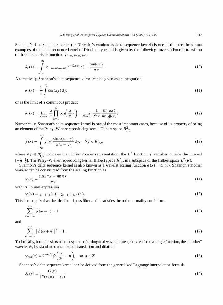
2.2. Fourier pseudospectral method

In this subsection, we present a brief description of the Fourier pseudospectral method by Sanders et al. [38].In general, spectral methods refer to all those global methods that can be interpreted as projection methods overa finite-dimensional space of polynomials with respect to an appropriate inner product. Three most importantspectral formulations are theGalerkin, tau, andcollocationmethods. The spectral method employed in the presentwork is the collocation scheme with the discrete Fourier basis as the trial functions and is referred as the Fourierpseudospectral (FPS) method [6,38,39].

In general, the Fourier pseudospectral method is implemented with the use of the periodic boundary conditions.A spatial domain,[0,Lx] × [0,Ly], is discretized intoNx andNy equidistance points in thex- andy-directionswith grid spacings%x = Lx/Nx and%y = Ly/Ny . The forward discrete Fourier transform (DFT) of a functionu(x, y, t) is defined as

ul,m =Nx−1∑j=0

Ny−1∑k=0

uj,ke2π i(lj/Nx+mk/Ny),

l = −Nx/2,−Nx/2+ 1, . . . ,Nx/2− 1; (37)

m= −Ny/2,−Ny/2+ 1, . . . ,Ny/2− 1

and its inverse discrete Fourier transform is given by

uj,k = 1

NxNy

Nx/2−1∑l=−Nx/2

Ny/2−1∑m=−Ny/2

ul,me−2π i(j l/Nx+km/Ny),

(38)j = 0,1, . . . ,Nx − 1; k = 0,1, . . . ,Ny − 1.

In the present periodic boundary condition, what is actually needed is not the Fourier expansion coefficients, but afast way to compute convolutions. The fast Fourier transform (FFT) is the natural solution and is thus used in thepresent work. As such, the number of the grid pointsNx andNy are taken to be the power of 2.

What is required for solving PDEs is the approximation of the differential operators. In the FPS methods, such anapproximation is given by algebraic multiplications. Ifu(x, y, t) is a sufficiently smooth function of its variables,its spatial derivatives can be evaluated as

[dnu

dxn

]j,k

= 1

NxNy

Nx/2−1∑l=−Nx/2

Ny/2−1∑m=−Ny/2

(2π il

Lx

)nul,me−2π i(j l/Nx+km/Ny),

(39)[dnu

dyn

]j,k

= 1

NxNy

Nx/2−1∑l=−Nx/2

Ny/2−1∑m=−Ny/2

(2π im

Ly

)nul,me−2π i(j l/Nx+km/Ny).

This global approximation is very efficient as long asNx andNy are not too large.

2.3. Temporal discretization

As the fourth-order Runge–Kutta (RK4) scheme is a robust approach for the temporal discretization, it isemployed for both the heat equation and the wave equation. However, the Navier–Stokes equation with theincompressible condition is an ill-posed problem and a Poisson equation for pressure is derived by using theincompressible condition. The resulting equations of velocity and pressure are updated by using the Crank–Nicolson scheme and details are given in the next section. Here, we describe the RK4 scheme.


For the time discretization of the heat and wave equations, we rewrite the spatially discretized Eq. (32) in itsmatrix form as

dudt

= F(u, t), (40)

where u is a vector having components [u11, u21, . . . , uNx1, u12, . . . , uNxNy ]T. The fourth-order Runge–Kuttascheme (RK4) is used to solve foru at each time stepn+ 1,

un+1 = un + 16(r1 + 2r2 + 2r3 + r4),

r1 =%tF(un, tn),

r2 =%tF(un + 1

2r1, tn + 12%t

),

r3 =%tF(un + 1

2r2, tn + 12%t

),

r4 =%tF(un + r3, tn +%t

). (41)

Except for specified cases, the RK4 is used in association with both the DSC algorithm and the FPS method in thepresent work.

2.4. Discrete Fourier analysis of the DSC kernels

In general, discrete Fourier basis isexact for time-independent problems whose solutions are given bybandlimited, periodicL2 functions. The use of discrete Fourier analysis for characterizing the errors ofdifference approximations has been extensively described [40–42]. Indeed, the Fourier analysis characterizesthe Fourier resolution of an interpolation or differential scheme applied to a class of bandlimited periodicfunctions. In this subsection, we discuss the discrete Fourier analysis of DSC kernels in association withthe approximation of bandlimited periodic functions and their derivatives. Such an analysis is to projectthe DSC kernel into the discrete Fourier basis. The result provides us an idea about accuracy of the DSCkernels used for bandlimited periodic functions. It is point out that such a result does not hold when thefunction is not bandlimited periodic. The analysis in this subsection is carried out in one-dimensional spatialcoordinate.

Using discrete Fourier analysis, the DSC kernel function, i.e. the RSK (35), and itsnth derivative{δ(n)α,σ (xj )}N−1j=0

can be transformed into the Fourier representationδ(n)α,σ (l)

δ(n)α,σ (l)=N−1∑j=0

δ(n)α,σ (xj )ei2πlj/N,

(42)l = −N/2,−N/2+ 1, . . . ,N/2− 1.

Here, δα,σ (l) are a set of low pass filter coefficients which are distributed over the discrete wave numbers{2πl/L}N/2−1

l=−N/2, i.e. the wave numbers that can be resolved range from−π/% to π/%. The quantityπ/% isthe Nyquist frequency, which is the maximum wave number that can be distinguished by the discretization withmesh size%. Similarly, δ(1)α,σ (l), δ

(2)α,σ (l), . . . are sets of high pass filter coefficients. For convenience, we introduce

a scaled wavenumberωl = 2πl%/L = 2πl/N and a scaled coordinatesj = xj/%. The Fourier modes in termsof these new definitions are simply exp(iωlsj ). Therefore, the domain of the scaled wavenumber is converted into[−π,π]. As such, the Dirichlet kernel generated from the discrete Fourier basis will be an ideal low pass filter inthe domain[−π,π], i.e. it is exact for periodicL2 functions bandlimited toπ . It is noted that all other spectralbases cannot give exact interpolation for periodicL2 functions bandlimited toπ .

For the first order derivative, the FPS provides the exact response function iω within the frequency band[−π,π].In Fig. 1, the response functions ofδ(1)σ,α(l) are plotted for a few differentM andr = σ/% values. WhenM = 16,


Fig. 1. The Fourier resolutions of the first order derivative approximated by using a few kernels.

the DSC kernel gives accurate response at relatively low frequency. As the frequency increases, the kernelresponse decreases gradually to zero. At a largerM value (M = 32), the DSC kernel gives accurate responseup to higher frequency components. The responses obtained at a few differentr values are depicted in Fig. 1.It appears that for a sufficiently largeM, the larger ther is, the better the response is. However, one has to bevery careful since errors that are smaller than 1% cannot be noticed from the plot. A more detailed plot, Fig. 2,indicates that if ther is too large, the accuracy of the DSC kernel might degrade. It is found that there existssome optimal range ofr, depending on the value ofM. In Fig. 2, the differences between the DSC responsesat M = 32 and the exact response are plotted for the parameterr being 4, 5, 6 and 7. As shown in the plot,the larger the value ofr, the better the approximation to high frequency will be. Therefore, it implies we canachieve a better approximation to the high frequency range when we use a large enoughr. However, there isa trade off between the accuracy for the high frequency part and that for the low frequency part. As seen fromFig. 2, the larger the value ofr, the larger the errors in the low frequency responses. Therefore, from Figs. 1and 2, it can be concluded that the optimal valuer should be chosen depending on the nature of problems tobe solved, and a compromise between the high frequency resolution and the low frequency resolution should beachieved.

Accuracy is one of the most important factors in choosing a computational method for a practical application.In the Fourier space, the FPS basis provides the most accurate (i.e. exact) representation. However, the sameFPS basis is not the best basis in a polynomial space, where the finite difference approximation can be provedto be the most accurate basis. Depending on the nature of problems under study, there exist different numericalmethods which are the most accurate. Although the DSC algorithm is not as accurate as the FPS method forapproximating bandlimited periodic functions, it can be more accurate than the FPS method for many otherproblems.


Fig. 2. The errors of a few kernels in approximating the first order derivative.

3. Results and discussion

In this section, we employ three two-dimensional (2D) problems, the heat equation, the wave equation, and theNavier–Stokes equation, to make a detailed comparison between the Fourier pseudospectral (FPS) method andthe DSC algorithm. The DSC algorithm is realized by using the regularized Shannon’s kernel (RSK) (35). Thespatial computational support in the DSC is set to 2M + 1, i.e. each local spatial grid makes use of the values ofits 2M nearest neighbors and the point itself. We take three values forM, 8, 16 and 32, to compare the accuracyand stability of the DSC and the FPS method. The FFT is utilized for the FPS method. The fourth-order Runge–Kutta (RK4) scheme is used for time integrations in solving the heat and the wave equations. For simplicity, wetake a square domain (Lx = Ly ) with the same number of grid points in each direction(N = Nx = Ny) in ourcomputations. For a fair comparison, both methods are tested with the same grid spacings% = %x = %y in thesquare domain.

To compare the accuracy of both methods, we calculate the errors of numerical approximationsu with respect tothe exact analytical solutionsu of each test problem. Two kinds of numerical error measures, i.e.L∞ andL2 errors,are used in this work. These error measures are defined asL∞ = max|uij −uij | andL2 = (%2 ∑

ij (uij −uij )2)1/2,

respectively. Some brief discussions are given based on the detailed comparison of both methods in terms ofaccuracy and stability.

3.1. The heat equation

We consider the 2D heat equation or diffusion equation

∂u(x, y, t)

∂t= a2

(∂2u(x, y, t)

∂x2 + ∂2u(x, y, t)

∂y2

). (43)

The heat equation is a good test problem because it admits an exact solution of the form


Fig. 3. Plot of solution of the heat equation at timet = 0.1 anda = 0.7. The figure on the right is the Fourier Transform of the left one.

Fig. 4. Plot of solution of the heat equation at timet = 1 anda = 0.7. The figure on the right is the Fourier Transform of the left one.

u(x, y, t)= 1

4a2πte−(x2+y2)/(4a2t ). (44)

Note that, the Fourier transform of Eq. (44) is still a Gaussian, i.e.

u(ωx,ωy, t)= 1√2π

∫ ∞∫−∞

u(x, y, t)eixωx+iyωy dx dy = 1

2πe−a2t (ω2

x+ω2y ). (45)

To utilize the FPS method for this problem, we have to cast the problem to a large computational domain so that theperiodic boundary condition is applicable. We consider the heat equation in a 2D square domain[0,10] × [0,10].The parametera in the heat equation (43) is set to 0.7 in all computations. Since it is difficult to accurately representthe initial condition, a delta pulse on a grid, we choose the initial value as the Gaussian wave att = 0.1

u0(x, y)= 1

4a2πte−[(x−x0)

2+(y−y0)2]/(4a2t ), (46)


Table 1Numerical solutions of the heat equation (%t = 0.001)

N t Periodical b.c. Dirichlet b.c.

FPS RSK-8 RSK-16 RSK-8 RSK-16

16 0.5 L2 2.69E−2 2.36E−2 2.61E−2 2.36E−2 2.61E−2

L∞ 2.45E−2 1.55E−2 2.15E−2 1.55E−2 2.15E−2

1.0 L2 1.36E−2 1.32E−2 1.36E−2 1.32E−2 1.36E−2

L∞ 7.62E−3 6.50E−3 7.48E−3 6.50E−3 7.48E−3

1.5 L2 1.00E−2 9.94E−3 1.00E−2 9.94E−3 1.00E−2

L∞ 4.30E−3 4.03E−3 4.29E−3 4.03E−3 4.29E−3

2.0 L2 8.29E−3 8.24E−3 8.29E−3 8.24E−3 8.29E−3

L∞ 2.97E−3 2.87E−3 2.97E−3 2.87E−3 2.97E−3


32 0.5 L2 1.93E−7 8.09E−6 2.36E−7 8.09E−6 2.36E−7

L∞ 1.70E−7 5.86E−6 9.81E−8 5.86E−6 9.81E−8

1.0 L2 9.12E−7 2.68E−7 2.45E−7 1.37E−7 7.96E−8

L∞ 4.69E−7 9.06E−8 9.06E−8 5.55E−8 2.89E−8

1.5 L2 5.08E−5 2.27E−5 2.26E−5 1.02E−5 1.01E−5

L∞ 2.20E−5 2.33E−6 7.34E−6 3.38E−6 3.34E−6

2.0 L2 3.72E−4 2.10E−4 2.10E−4 1.14E−4 1.13E−4

L∞ 1.38E−4 6.06E−5 6.06E−5 3.36E−5 3.33E−5

where the point(x0, y0) is the center of the 2D square domain. This initial value is depicted in Fig. 3 (a = 0.7). TheFourier transform of the Gaussian initial wave is also shown in Fig. 3. The corresponding plots ofu(x, y, t = 1) inboth the coordinate space and the Fourier space are shown in Fig. 4. As can be seen from these plots, the Gaussianwave grows wider as time increases, whereas the corresponding Fourier transform of the Gaussian wave becomesnarrower as time increases.

We use both the DSC and FPS methods to approximate the 2nd order derivatives in Eq. (43). The DSCdiscretization (34) of the heat equation is given as

duijdt

= a2

[i+M∑k=i−M

δ(2)α,σ (xi − xk)+j+M∑l=j−M

δ(2)α,σ (yj − yl)

]ui,j . (47)

The DSC algorithm is implemented with both periodic and Dirichlet boundary conditions (b.c.). Here, the Dirichletboundary condition assumes that the function values outside the boundaries of 2D domain[0,10]× [0,10] vanish.We use the RK4 scheme (41) for the time integration of above (47) to solve for a set ofuij at each time step. Timeincrement used in our computations is usually very small so that most errors are due to spatial discretizations. Thetime integration cannot be too long for this problem so as to avoid significant boundary effects.

The computational errors with respect to the exact solution are listed in Tables 1 and 2. The FPS methodis compared with the DSC algorithm with both the periodic and Dirichlet boundary conditions. Both the time


Table 2Numerical solutions of the heat equation (%t = 0.01)

N t Periodical b.c. Dirichlet b.c.


16 0.5 L2 2.69E–2 2.36E–2 2.61E–2 2.36E–2 2.61E–2

L∞ 2.44E–2 1.55E–2 2.15E–2 1.55E–2 2.15E–2

1.0 L2 1.36E–2 1.32E–2 1.36E–2 1.32E–2 1.36E–2

L∞ 7.62E–3 6.50E–3 7.48E–3 6.50E–3 7.48E–3

1.5 L2 1.00E–2 9.94E–3 1.00E–2 9.94E–3 1.00E–2

L∞ 4.13E–3 4.03–E3 4.29E–3 4.03–E3 4.29E–3

2.0 L2 8.29E–3 8.24E–3 8.28E–3 8.24E–3 8.28E–3

L∞ 2.97E–3 2.87E–3 2.97E–3 2.87E–3 2.97E–3


32 0.5 L2 2.35E–7 8.06E–6 2.64E–7 8.05E–6 2.64E–7

L∞ 2.16E–7 5.82E–6 1.05E–7 5.82E–6 1.05E–7

1.0 L2 9.12E–7 2.67E–7 2.45E–7 1.35E–7 8.00E–7

L∞ 4.69E–7 9.06E–8 9.06E–8 5.40E–8 2.89E–8

1.5 L2 5.08E–5 2.26E–5 2.26E–5 1.02E–5 1.01E–5

L∞ 3.72E–4 2.10E–4 2.10E–4 1.22E–4 1.21E–4

2.0 L2 1.49E–3 1.14E–4 1.13E–4 6.66E–4 6.62E–4

L∞ 1.38E–4 6.06E–5 6.06E–5 3.36E–5 3.33E–5

increment%t and the number of grid pointsN are varied to test the performance of both methods. We employ anequal spatial discretization alongx- andy-directions, i.e.N =Nx =Ny . AlthoughN can take any integer value inthe DSC algorithm, in order to compare with FPS in whichN is required to be powers of 2, we chooseN = 16 andN = 32 for our computations. In the DSC scheme, we have one more parameterM which determines the supportsize of the DSC kernels. The value ofM is usually set smaller thanN , therefore we chooseM = 8 andM = 16.The corresponding DSC methods are referred to as RSK-8 and RSK-16, respectively.

From Tables 1 and 2, we observe that the DSC with the periodic boundary condition gives the same order ofaccuracy as the FPS (see the RSK-16 with periodic b.c. and the FPS in Table 2). The comparison has been donefor two time steps%t = 0.001 and%t = 0.01 with two spatial discretizationsN = 16 andN = 32. The resultsindicate that, DSC algorithm is competitive with the FPS method.

Moreover, a careful comparison indicates that the boundary condition used in the DSC algorithm affects theaccuracy of the method. As in Tables 1 and 2, all the RSK-8, RSK-16 and RSK-32 with the Dirichlet boundarycondition are similar to the corresponding DSC schemes with the periodical boundary condition, and more accuratethan the FPS method with the sameN value. The importance of boundary condition is most obvious for a largerN value. Note that, for a large enoughN = 32, the support sizeM has less effect on the accuracy of the DSCalgorithm in this problem. The dominant factor that affects the accuracy of the DSC algorithm is the boundarycondition atN = 32.


Obviously, as a local method, the DSC algorithm is more robust than the FPS method in choosing the numberof grid points, and in dealing with complex geometry and boundary condition. However, it is not so obvious whythe DSC algorithm is even more accurate than the FPS method for the heat equation. In general, global methodsshould be more accurate than local ones. Indeed, we have shown in the last section that the discrete Fourier basis ismore accurate than the DSC kernels. In the present case, the solution of the heat equation is the Gaussian which isinvariant with respect to the Fourier transform, i.e. it is also a Gaussian in the Fourier domain as shown in Eq. (45).As a result, the Gaussian is not bandlimited, nor is it periodic. In such a case, the FPS method does not provide oneof the best approximations for solving the heat equation. In contrast, the DSC algorithm is indeed not as accurateas the FPS method for approximating the bandlimited periodic function as illustrated by the earlier discrete Fourieranalysis. However, for some non-bandlimited functions, the DSC algorithm turns out to be more accurate.

3.2. The wave equation

Propagation of electromagnetic wave is governed by Maxwell’s equations. In a charge-free homogeneousmedium, the wave equation can be used to describe the motion of an electric or magnetic field. For simplicity,we consider the 2D wave equation of the form

∂2u(x, y, t)

∂t2= v2

(∂2u(x, y, t)

∂x2+ ∂2u(x, y, t)

∂y2

), (48)

wherev is the velocity of the wave. A general solution to Eq. (48) has form off (x ± y ± vt).The wave equation is different from the heat equation (43) due to the second order derivative in time. To use the

RK4 scheme (41) for the time evolution of Eq. (48), we rewrite the wave equation as two coupled PDEs

∂w(x, y, t)

∂t= v2

(∂2u(x, y, t)

∂x2+ ∂2u(x, y, t)

∂y2

),

(49)∂u(x, y, t)

∂t= w(x,y, t).

The spatial discretizations using both the FPS method and the DSC algorithm are described in Section 2.In our computation, we set the velocityv = 1.0 in all test cases. The computational domain is set to

[0,2π] × [0,2π], on which the periodic boundary condition is imposed. We choose the initial condition asu(x, y,0)= cos(x + y) and thus, the exact solution of the wave equation (48) is given by

u(x, y, t)= cos(x + y + vt). (50)

Both the DSC and FPS methods are employed to compute the numerical solution of the wave equation (48)and their performance is compared. In Fig. 5, the waveform of the solution is plotted. Two types of spatialdiscretizations (N = 32 andN = 64) and time increments (%t = 0.0005 and%t = 0.01) are considered in ournumerical tests. The computational errors with respect to the exact solution (50) are listed in Table 3.

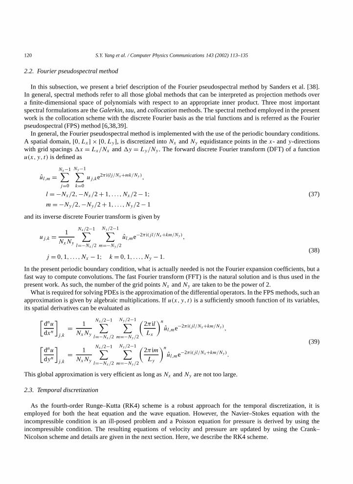
The results in the first part of Table 3 are obtained with a very small time increment(%t = 0.005) so that allerrors are mainly originated from the spatial discretization. The comparison is done for the timet up to 100. It isseen that whenM = 32, both the DSC and the FPS give the same order of accuracy and both methods can achievethe machine precision. Next, we consider a slightly larger time increment (%t = 0.01). We still observe that theaccuracy of both the DSC and the FPS is of the same order as shown in second part of Table 3.

Another important parameter is the support sizeM in the DSC kernel. The accuracy of the DSC algorithm iscontrollable by adjusting theM value. It is seen that the DSC algorithm is very accurate whenM = 16. In fact, itachieves machine precision with a large support sizeM = 32 at a small time increment (%t = 0.0005). However, ata large time increment (%t = 0.01), all the three schemes, the FPS, the RSK-16 and the RSK-32, give same orderof accuracy, and the choice ofM does not affect the accuracy of the DSC algorithm. This is due to the fact that, fora large%t , the main errors come from the time discretization.


Fig. 5. The solution of the wave equation.

3.3. The Navier–Stokes equation

The Navier–Stokes (NS) equation is the governing equation for aerodynamics and fluid dynamics and hasapplications in various problems, including weather forecasting, turbulence simulation, and chemical reaction,etc. Some of these problems invoke complicated boundary conditions, which cause difficulties for global methods,including the FPS method. There is no general analytical solution to the Navier–Stokes equation, except for afew simple cases. Recently, the DSC algorithm has been employed to solve the Navier–Stokes equation withsimple [23] and complex geometries [25]. In this work, we consider the Taylor problem, i.e. the Navier–Stokesequation with periodic boundary conditions, to make a comparison of the DSC and FPS methods. This problemadmits an analytical solution and can be solved by using both the FPS and the DSC, and thus, the performance ofboth methods can be compared in detail. Both approaches are formulated in association with the Crank–Nicolsonscheme.

3.3.1. The problem and solution schemeWe consider the Navier–Stokes equation in its primitive variable, describing an incompressible fluid flow

∂u∂t

+ u · ∇u = −∇p+ 1

Re∇2u, (51)

∇ · u = 0, (52)

whereu = (u, v) is the velocity vector having itsx- andy-componentsu(x, y, t) andv(x, y, t), respectively. Here,p is the pressure. We are interested in the Navier–Stokes equation with periodic boundary conditions, i.e. the Taylorproblem, in a 2D square domain[0,2π] × [0,2π]. The initial values for the velocity are taken as

u(x, y,0)= −cos(kx)sin(ky),(53)

v(x, y,0)= sin(kx)cos(ky),


Table 3Errors of the numerical solutions of the wave equation

%t = 0.0005

N t L2 L∞RSK-16 RSK-32 FPS RSK-16 RSK-32 FPS

64 0.1 3.02E–11 3.02E–15 2.79E–15 6.73E–12 2.11E–15 1.78E–15

1 2.72E–09 2.30E–13 2.44E–13 6.02E–10 5.31E–14 5.69E–14

10 2.90E–08 3.59E–12 3.32E–12 6.43E–09 8.01E–13 7.43E–13

100 3.01E–07 1.34E–09 1.34E–09 6.73E–08 2.96E–10 2.95E–10

32 0.1 3.96E–11 3.08E–15 1.87E–15 8.63E–12 1.67E–15 7.49E–16

1 3.54E–09 2.15E–13 2.42E–13 7.72E–10 4.77E–14 5.60E–14

10 3.78E–08 4.07E–12 3.27E–12 8.24E–09 8.93E–13 7.38E–13

100 3.97E–07 1.36E–09 1.31E–09 8.65E–08 2.97E–10 2.95E–10

%t = 0.01

64 0.1 4.69E–11 3.76E–11 3.70E–11 1.04E–11 8.33E–12 8.33E–12

1 2.51E–09 3.76E–10 3.70E–10 5.56E–10 8.33E–11 8.33E–11

10 2.53E–08 3.76E–09 3.70E–09 5.60E–09 8.33E–10 8.33E–10

100 2.68E–07 3.77E–08 3.71E–08 5.93E–08 8.35E–09 8.34E–09

1000 2.67E–06 3.73E–07 3.67E–07 5.91E–07 8.26E–08 8.26E–08

32 0.1 5.34E–11 3.82E–11 3.70E–11 1.16E–11 8.33E–12 8.30E–12

1 3.33E–09 3.82E–10 3.70E–10 7.25E–10 8.33E–11 8.33E–11

10 3.40E–08 3.82E–09 3.70E–09 7.41E–09 8.33E–10 8.33E–10

100 3.60E–07 3.83E–08 3.71E–08 7.84E–08 8.35E–09 8.34E–09

1000 3.58E–06 3.79E–07 3.67E–07 7.81E–07 8.26E–08 8.26E–08

wherek is the wavenumber taking an integer value. The case ofk = 1 was treated by using the DSC algorithm [23].In this work, we study the cases fork � 1 which involve higher frequency. The corresponding numerical solutionis compared with the exact one

u(x, y, t)= −cos(kx)sin(ky)e−2k2t/Re,

v(x, y, t)= sin(kx)cos(ky)e−2k2t/Re, (54)

p(x, y, t)= −14

[cos(2kx)+ cos(2ky)

]e−4k2t/Re.

We adopt the Adams–Bashforth–Crank–Nicolson (ABCN) scheme [43] for the time discretization and treatmentof pressure

1

2Re∇2un+1 − 1

%tun+1 = ∇pn+1/2 + Sn,

(55)∇2pn+1/2 + ∇ · Sn = 0,

where the source vectorSn is given by


Fig. 6. The solutions of the NS equation (k = 1 and Re= 100). Left:t = 1; right t = 30.

Sn = − un

%t+ 3(un · ∇)un − (un−1 · ∇)un−1

2− 1

2Re∇2un. (56)

The aspect of ensuring divergence-free velocity field in the scheme was discussed by Le Queéré and Alziary deRoquefort [44]. The error expression,L∞, is calculated to evaluate the accuracy of both numerical methods as inthe previous two numerical problems. Our calculations are conducted for a variety of Reynolds number Re,k andtime increment.

3.3.2. Numerical experimentsTwo algorithms, the DSC and the FPS, are applied to solve the NS equation for different values ofk from 1

to 5. In each case, Reynolds number Re varying from 100 to 1010 is used in computation. We also compare thetwo algorithms for different time increment%t and spatial discretizationN . Here, for simplicity, we set equalspatial discretization inx- andy-directions. AlthoughN can be set to any integer values for the DSC algorithm,for the purpose of comparing with the FPS in whichN is required to be powers of 2, we chooseN = 32 in ourcomputations. Numerical solutions to the NS equation are obtained for a long time. In the DSC algorithm, wehave one more parameterM which determines the support size of DSC kernels. The value ofM is usually smallerthanN , therefore we chooseM = 16 or 32. The corresponding DSC algorithm are denoted by the RSK-16 andRSK-32, respectively.

The solutions of the present problem are of sin(kx) and cos(kx) type, which are the basis functions of Fourierpseudospectral methods. The periodic boundary conditions are also suitable for the FPS method. Therefore, it isexpected that the FPS should achieve the highest possible accuracy in this case.

We first study the case ofk = 1 in Eq. (55). The solutionsu(x, y, t) (55) of the NS equation at timet = 1 andt = 30 are depicted in Fig. 6. TheL∞ errors of the numerical results obtained using the DSC and FPS methods fortime up to 30 are listed in Table 4. The number of grid points is set asN = 32 in each dimension, and the resultsobtained by using the FPS is compared with those of the RSK-16 and RSK-32.

For the case of Re= 1010, it is observed in Table 4 that the accuracy of the DSC algorithm depends on thechoice of support sizeM, as the DSC algorithm is a local method. We have shown again that the accuracy ofthe DSC algorithm is controllable. The DSC algorithm becomes more accurate as the support sizeM increasesfrom 16 to 32. It is interesting to note that the RSK-32 is even more accurate than the FPS method for both timeincrements. In the same table, the computations are shown for smaller Reynolds numbers. For two intermediateReynolds numbers, the FPS method performs slightly better than the DSC algorithm, as in the same table. In


Table 4L∞ error of the numerical solutions for the NS equation withk = 1

Re t %t = 0.001 %t = 0.01

RSK-16 RSK-32 FPS RSK-16 RSK-32 FPS

102 1 1.27E–07 1.80E–12 1.95E–10 1.26E–07 6.53E–11 1.95E–08

10 1.06E–06 1.03E–11 1.52E–10 1.01E–06 5.46E–10 1.58E–08

20 1.74E–06 1.42E–11 1.15E–10 1.64E–06 8.94E–10 1.25E–08

30 2.11E–06 1.54E–11 8.68E–11 1.99E–06 1.08E–09 1.01E–08

104 1 2.91E–09 1.37E–12 7.91E–13 3.51E–08 2.27E–13 1.93E–12

10 2.02E–08 2.84E–11 7.59E–12 2.67E–07 5.13E–12 1.30E–12

20 4.01E–08 1.11E–10 1.48E–11 5.31E–07 2.38E–11 6.87E–13

30 5.77E–08 2.05E–10 2.23E–11 7.65E–07 7.39E–11 5.68E–13

106 1 3.58E–09 7.38E–13 9.02E–13 3.57E–08 1.53E–13 8.89E–14

10 2.75E–08 1.18E–11 8.65E–12 2.76E–07 4.00E–12 8.46E–13

20 5.51E–08 5.85E–11 1.70E–11 5.52E–07 3.80E–11 1.66E–12

30 7.99E–08 1.38E–10 2.56E–11 8.01E–07 1.70E–10 2.46E–12

1010 1 3.59E–09 2.96E–13 9.9-E–13 3.57E–08 2.75E–14 9.90E–14

10 2.76E–08 2.18E–12 9.46E–12 2.76E–07 2.49E–13 9.42E–13

20 5.52E–08 4.47E–12 1.86E–11 5.52E–07 5.68E–13 1.83E–12

30 8.01E–08 6.50E–12 2.79E–11 8.28E–07 9.28E–13 2.70E–12

these three cases, the results obtained from%t = 0.01 are generally better than those from%t = 0.001 for boththe RSK-32 and the FPS. This phenomenon follows naturally from the fact that at a high Reynolds number, thesolution does not vary much with time. Therefore, the numerical solution is not so sensitive to the size of the timeincrement%t . A larger time increment implies a smaller number of iterations to reach a given total time, whichleads to higher accuracy. When the Reynolds number is reduced to 100, as expected, a smaller time incrementyields higher accuracy for both methods. In this case, the DSC algorithm outperforms the FPS method again. It isobvious that both methods perform extremely well for this case.

We next consider the case ofk = 2. The solutionsu(x, y, t) (55) of the NS equation at timet = 1 andt = 30are plotted in Fig. 7. TheL∞ errors obtained by both the FPS and DSC are given in Table 5. Similar to theprevious case, the numerical study is performed at two different time increments%t = 0.001 and%t = 0.01 forfour Reynolds numbers Re= 1010, 106, 104 and 100.

We observe that, for small value oft (t < 10), both the RSK-32 and the FPS give similar order of accuracy.However, whent is large and approaches 30, the DSC scheme gives much better results than the FPS does. Thishappens for both time increments%t = 0.001 and 0.01. For example, The DSC algorithm performs about a 1000times better than the FPS att = 30. At a low Reynolds number, Re= 100, the DSC algorithm still performs100 times better than the FPS method at early times. However, both the FPS and the DSC give the same level ofaccuracy at a late timet = 30. It is noted that the factor e−2k2t/Re in the analytical solution (55) becomes verysmall for largek and/ort , and small Re. Therefore, the small errors in both methods are in part due to the smallmagnitude of the exact solutions of the NS equation.


Fig. 7. The solutions of the NS equation withk = 2 and Re= 100. The left plot is the solution at timet = 1. The right plot is the one attime t = 30.


Re t %t = 0.001 %t = 0.01

RSK-32 FPS RSK-32 FPS

102 1 4.01E–11 2.91E–09 3.93E–09 2.91E–07

10 1.93E–10 1.24E–09 1.91E–08 1.25E–07

20 1.74E–10 4.72E–10 1.72E–08 4.74E–08

30 1.24E–10 1.73E–10 1.21E–08 1.74E–08

104 1 9.32E–13 3.33E–13 1.82E–13 3.19E–11

10 4.51E–11 6.64E–12 6.78E–12 3.13E–11

20 1.39E–09 4.41E–09 4.50E–10 5.91E–10

30 5.99E–08 4.07E–06 3.12E–08 9.55E–07

106 1 5.07E–13 5.28E–13 8.59E–14 5.01E–14

10 1.76E–11 7.36E–12 5.36E–12 1.34E–12

20 3.99E–10 3.80E–09 3.45E–10 1.38E–09

30 1.71E–08 4.99E–06 2.38E–08 3.17E–06

1010 1 4.20E–13 5.94E–13 8.63E–14 3.97E–14

10 5.09E–12 6.65E–12 1.02E–12 1.14E–12

20 6.41E–11 4.58E–09 1.61E–11 1.05E–09

30 2.33E–09 6.99E–06 1.00E–09 1.42E–06

Finally, we consider the case ofk = 5. Obviously, this case requires very high spatial accuracy (or Fourierresolution). In all the previous cases, the parameterσ = 3.2% is used as it gives very accurate approximations.However, in the present case, a largeσ value is required to take better care of the high frequency component.



Re t %t = 0.001 %t = 0.01

RSK-32 FPS RSK-32 FPS

102 1 6.53E–09 6.95E–08 6.32E–07 6.93E–06

10 7.25E–10 1.40E–10 7.02E–08 1.38E–08

20 9.79E–12 3.79E–12 9.46E–10 3.80E–10

104 1 4.25E–11 1.18E–11 4.01E–10 1.24E–09

10 1.18E–06 1.38E–06 1.41E–06 1.41E–07

106 1 4.10E–11 1.15E–12 4.06E–10 7.32E–14

10 7.37E–07 1.86E–06 2.16E–06 5.83E–07

1010 1 4.07E–11 1.02E–12 4.06E–10 7.32E–14

10 4.95E–07 2.49E–06 2.11E–06 5.83E–07

Therefore, we chooseσ = 5.4%. Whenσ = 5.4%, though the DSC algorithm approximates higher frequency partbetter, it is at the sacrifice of the accuracy for approximating low frequency components as seen from Fig. 2. InTable 6, we compare the accuracy of the RSK-32 and the FPS atk = 5. At high Reynolds numbers, the system isdominated by the nonlinear advection. The accuracy of both methods degrades quite fast. It is seen that the FPSmethod performs slightly better than the DSC algorithm. It also can be observed that, for small Reynolds number,the DSC algorithm can compete with the FPS method.

As a short summary of this section, the numerical study on the NS equation with periodic boundary conditionusing both the FPS and DSC methods shows that the DSC can compete with the FPS method in terms of accuracy,though the problem is most suitable for the implementation of the FPS method. This point has been illustratedby using various choices of time increment%t , Reynolds number Re and wavenumberk for arbitrarily long timeevolutiont . Moreover, we have demonstrated that the accuracy of the DSC algorithm is controllable.

4. Conclusion

In this work, we explore the utility, test accuracy and examine the limitation of the discrete singular convolution(DSC) algorithm for solving three types of partial differential equations (PDEs). Particular attention has been givento a detailed comparison of the DSC algorithm and the Fourier pseudospectral (FPS) method for computationalaccuracy and stability. To this end, three two-dimensional PDEs of different nature, the heat equation, the waveequation and the Navier–Stokes equation are solved by using both methods with standard temporal discretizations,i.e. the fourth-order Runge–Kutta or Crank–Nicolson scheme. The numerical resolution of the DSC algorithmfor approximating the spatial derivatives is analyzed by using the discrete Fourier analysis. Extensive numericalexperiments are conducted at a variety of time increment, grid spacing, wavenumber, and Reynolds number (for theNavier–Stokes equation) to give a comprehensive comparison between the two methods. The substantial numericalresults lead to convincing conclusions which are summarized as follows:

(1) There is no doubt that the FPS method gives the most accurate spatial discretization for problems involvingbandlimited periodicL2 functions. The DSC algorithm is not as accurate as the FPS method for the highfrequency component of such functions. However, DSC can perform better than FPS method in many otheraspects.


(2) The accuracy of the DSC algorithm is controllable by adjusting its support parameterM. At a largeM,the DSC algorithm can be even more accurate than the FPS method for approximating non-bandlimitedfunctions, such as the Gaussian solution to the heat equation, and can be nearly as accurate as the FPSmethod for bandlimited periodic functions, such as those in the wave equation and the Taylor problem.

(3) The DSC algorithm can be used as both local and global methods depending on the choice of theparameterM. As a result, it can be used for treating complex geometry and boundary conditions, whereas,the FPS method is a global method and is generally restricted to treating periodic boundary conditions. TheDSC algorithm has been proved useful in treating complex boundary conditions in structural analysis [22,29,31] and complex geometries in handling flow simulations [25].

(4) The number of grid points is limited to the power of 2 in the FPS method. There is no such a limitation inthe DSC algorithm.

(5) The FPS method in association with the FFT algorithm, is faster than the DSC algorithm when the grid isnot very large. For approximating a derivative, the operation of the FFT is proportional toN logN (hereNis the total number of grid points), whereas, the operation for DSC algorithm isN(2M + 1). We found thatwhenN = 512, the DSC algorithm becomes faster than the FPS method.

Acknowledgement

This work was supported in part by the National University of Singapore.

References

[1] C. Lanczos, Trigonometric interpolation of empirical and analytical functions, J. Math. Phys. 17 (1938) 123–199.[2] J.W. Cooley, J.W. Tukey, An algorithm for the machine calculation of complex Fourier series, Math. Comput. 19 (1965) 297–301.[3] B.A. Finlayson, L.E. Scriven, The method of weighted residuals—a review, Appl. Mech. Rev. 19 (1966) 735–748.[4] S.A. Orszag, Comparison of pseudospectral and spectral approximations, Stud. Appl. Math. 51 (1972) 253–259.[5] C. Canuto, M.Y. Hussaini, A. Quarteroni, T.A. Zang, Spectral Methods in Fluid Dynamics, Springer, Berlin, 1988.[6] B. Fornberg, A Practical Guide to Pseudospectral Methods, Cambridge University Press, Cambridge, 1996.[7] L.N. Trefethen, Spectral Methods in Matlab, Oxford University, Oxford, England, 2000.[8] G.E. Forsythe, W.R. Wasow, Finite-Difference Methods for Partial Differential Equations, Wiley, New York, 1960.[9] E. Isaacson, H.B. Keller, Analysis of Numerical Methods, Wiley, New York, 1966.

[10] O.C. Zienkiewicz, The Finite Element Method in Engineering Science, McGraw-Hill, London, 1971.[11] C.S. Desai, J.F. Abel, Introduction to the Finite Element Methods, Van Nostrand Reinhold, New York, 1972.[12] J.T. Oden, The Finite Elements of Nonlinear Continua, McGraw-Hill, New York, 1972.[13] B. Nath, Fundamentals of Finite Elements for Engineers, Athlone Press, London, 1974.[14] R.T. Fenner, Finite Element Methods for Engineers, Imperial College Press, London, 1975.[15] Y.K. Cheung, Finite Strip Methods in Structural Analysis, Pergamon Press, Oxford, 1976.[16] S.S. Rao, The Finite Element Method in Engineering, Pergamon Press, New York, 1982.[17] J.N. Reddy, Energy and Variational Methods in Applied Mechanics, John Wiley, New York, 1984.[18] G.W. Wei, Discrete singular convolution for the Fokker–Planck equation, J. Chem. Phys. 110 (1999) 8930–8942.[19] G.W. Wei, A unified approach for solving the Fokker–Planck equation, J. Phys. A 33 (2000) 4935–4953.[20] G.W. Wei, Wavelets generated by using discrete singular convolution kernels, J. Phys. A 33 (2000) 8577–8596.[21] G.W. Wei, Solving quantum eigenvalue problems by discrete singular convolution, J. Phys. B 33 (2000) 343–352.[22] G.W. Wei, Vibration analysis by discrete singular convolution, J. Sound Vibration 244 (2001) 535–553.[23] G.W. Wei, A new algorithm for solving some mechanical problems, Comput. Methods Appl. Mech. Engrg. 190 (2001) 2017–2030.[24] G.W. Wei, A unified method for computational mechanics, in: C.M. Wang, K.H. Lee, K.K. Ang (Eds.), Computational Mechanics for the

Next Millennium, Elsevier, New York, 1999, pp. 1049–1054.[25] D.C. Wan, G.W. Wei, Discrete singular convolution-finite subdomain method for the solution of incompressible viscous flows, J. Comput.

Phys., in press.[26] S. Guan, C.-H. Lai, G.W. Wei, Bessel–Fourier analysis of patterns in a circular domain, Physica D 151 (2001) 83–98.[27] G.W. Wei, Synchronization of single-side averaged coupling and its application to shock capturing, Phys. Rev. Lett. 86 (2001) 3542–3545.


[28] G.W. Wei, Discrete singular convolution method for the sine-Gordon equation, Physica D 137 (2000) 247–259.[29] G.W. Wei, Discrete singular convolution for beam analysis, Engrg. Structures 23 (2001) 1045–1053.[30] G.W. Wei, Y.B. Zhao, Y. Xiang, The determination of the natural frequencies of rectangular plates with mixed boundary conditions by

discrete singular convolution, Int. J. Mech. Sci. 43 (2001) 1731–1746.[31] Y.B. Zhao, G.W. Wei, Y. Xiang, Plate vibration under irregular internal supports, Int. J. Solids Structures, in press.[32] G.W. Wei, Y.B. Zhao, Y. Xiang, Discrete singular convolution and its application to the analysis of plates with internal supports. I. Theory

and algorithm, Int. J. Numer. Methods Engrg., in press.[33] L. Schwartz, Theore des Distribution, Hermann, Paris, 1951.[34] G.W. Wei, Quasi wavelets and quasi interpolating wavelets, Chem. Phys. Lett. 296 (1998) 215–222.[35] G.G. Walter, J. Blum, Probability density estimation using delta sequences, Ann. Statist. 7 (1979) 328–340.[36] B.A. Finlayson, The Method of Weighted Residuals and Variational Principles, Academic, New York, 1972.[37] J.O. Dow, A Unified Approach to the Finite Element Method and Error Analysis Procedures, Academic, San Diego, CA, 1999.[38] B.F. Sanders, N.O. Katoposes, J.P. Boyd, Spectral modeling of nonlinear dispersive waves, J. Hydraulic. Engrg. ASCE 124 (1998) 2–12.[39] H.-O. Kreiss, J. Oliger, Comparison of accurate methods for the integration of hyperbolic systems, Tellus 24 (1972) 199–215.[40] K.V. Roberts, N.O. Weiss, Math. Comput. 20 (1966) 272.[41] B. Swartz, B. Wendroff, The relation between the Galerkin and collocation methods using smooth splines, SIAM J. Numer. Anal. 11

(1974) 994.[42] R. Vichnevetsky, J.B. Bowles, Fourier Analysis of Numerical Approximations of Hyperbolic Equations, SIAM, Philadelphia, 1982.[43] H.H. Yang, B. Shizgal, Chebyshev pseudospectral multi-domain technique for viscous flow calculation, Comput. Methods Appl. Mech.

Engrg. 118 (1994) 47.[44] P. Le Quéré, T. Alziary de Roquefort, Computation of natural convection in two-dimension cavities, J. Comput. Phys. 57 (1985) 210.

Comparison of the discrete singular convolution algorithm ...yzhou/papers/ZhouY2001a.pdf · for...

Documents

Transcript of Comparison of the discrete singular convolution algorithm ...yzhou/papers/ZhouY2001a.pdf · for...