Comparison of risk assessment methods for polluted …764650/FULLTEXT01.pdf · Comparison of risk...

Master’s thesisPhysical Geography and Quaternary Geology, 30 Credits

Department of Physical Geography and Quaternary Geology

Comparison of risk assessment methods for polluted soils in Sweden, Norway and Denmark

Viktor Plevrakis

NKA 1052014

Preface

This Master’s thesis is Viktor Plevrakis' degree project in Physical Geography and Quaternary

Geology at the Department of Physical Geography and Quaternary Geology, Stockholm

University. The Master’s thesis comprises 30 credits (one term of full-time studies).

Supervisor has been Jerker Jarsjö at the Department of Physical Geography and Quaternary

Geology, Stockholm University. Extern supervisor has been Johanna Moreskog, URS Nordic.

Examiner has been Andrew Frampton at the Department of Physical Geography and

Quaternary Geology, Stockholm University.

The author is responsible for the contents of this thesis.

Stockholm, 19 November 2014

Lars-Ove Westerberg

Director of studies

i

Abstract

Land contamination is an acknowledged problem around the world due to its

potentially adverse impacts on human health and the environment. Specifically in

Europe there are estimated to be 2,500,000 potentially contaminated sites. The risk

that contaminated sites pose is investigated by risk assessments. The methods and

the models though used in risk assessments, vary both on a national and an

international level.

In this study, the risk assessment methods and models for polluted soils used in

Scandinavia and issued by the Environmental Protection Agencies were compared.

The comparison aimed to (i) identify similarities and differences in the risk

assessment methodology and risk assessment methods and to (ii) investigate to

which extend these differences can impact the results of the models and the

implications regarding mitigation measures.

The method and model comparison showed that Sweden and Norway have great

similarities in assessing risks for contaminated soil. However, there are differences

with Denmark on a conceptual level. When a common hypothetical petrol station

with 20 soil samples was assessed, the results and the conclusions of the three risk

assessments were quite different; the site was seen as posing risk to human health

with the Danish model when complied with the quality criteria issued by the

Norwegian model. The Swedish risk assessment concluded that the contaminant

concentration in 3 out of 20 samples was potentially harmful for the environment but

not for human health.

The demonstrated divergence of the conclusions of risk assessments has major

implications and shows great interest for mainly four groups: Land-owners who may

be called to cover the expenses for remedial action. Consultants and companies who

perform risk assessments and land remediation. The countries that have to meet

national and international environmental goals and can also share/ or cover the cost

for remedial action. The people exposed to such environments that could be deemed

as potentially harmful by a neighboring country.

The study was conducted in collaboration with URS Nordic.

ii

Acknowledgments

First of all, I would like to express my gratitude to my two supervisors Jerker Jarsjö

and Johanna Moreskog for the supervision and guidance throughout my thesis.

Jerker has provided me great support at all different levels of our collaboration and

helped me overcome the various difficulties that came up during the thesis. Johanna

opened the door for me to URS Nordic by suggesting the research topic and

contributed with her deep understanding and knowledge on risk assessments.

Big thanks goes also to URS Nordic for allocating time and resources to train me,

transfer knowledge and providing me an office to work in the beginning of my

thesis. Ken Jenkins has been the first person that I met from URS Nordic and who

understood the benefits of a potential collaboration of Stockholm University and

URS. I am grateful that he facilitated to start this project. I would like to thank all the

employees of URS Nordic for the fruitful discussions around risk assessments in

Scandinavia but especially Åsa Lindström, Nicklas Gingborn and Sophie Andersson

who helped me with specific parts of the models. Furthermore, I want to thank Sanne

Arildsen who has offered substantial help to topics around the Danish risk

assessment methodology. The support of Aidin Geranmayeh when I was trying to

put all the pieces together is likewise highly appreciated. Our vigorous discussions

helped me to clarify critical aspects of risk assessments.

Finally, I would like to thank my family who has supported me over this two-year

period of my studies and encouraged me to take the next step in my education.

iii

Table of Contents

List of Abbreviations ............................................................................................................. iv

1. Introduction ....................................................................................................................... 1

1.1. Aims of the study....................................................................................................... 3

2. Background information to Risk Assessments .................................................................. 3

2.1. Swedish and Norwegian Risk Assessments .............................................................. 4

2.2. Danish Risk Assessment............................................................................................ 9

3. Methods ........................................................................................................................... 11

3.1. Case study ................................................................................................................ 11

3.1.1. Site description .............................................................................................. 11

3.1.2. CSM and model parameterization ................................................................. 13

3.1.3. Influence of each exposure pathway – conservation goal on site .................. 15

3.1.4. Analysis of the exposure path of consumption of groundwater .................... 16

4. Results ............................................................................................................................. 16

4.1. Method and model comparison ............................................................................... 17

4.2. Case study ................................................................................................................ 18

4.2.1. Compliance of the field concentrations with the quality criteria and

recognition of most influential paths ............................................................................. 18

4.2.2. Analysis of the exposure path of consumption of groundwater .................... 23

5. Discussion ....................................................................................................................... 25

5.1. Method and model comparison ............................................................................... 25

5.2. Case study ................................................................................................................ 27

5.3. Importance of the results ......................................................................................... 29

5.4. Potential sources of errors and limitations of the results ......................................... 31

4. Conclusions ..................................................................................................................... 32

5. References ....................................................................................................................... 34

6. Appendix ......................................................................................................................... 39

iv

List of Abbreviations

CES – Classes of Environmental State

CSM – Conceptual Site Model

EPA – Environmental Protection Agency

IGV – Individual Guideline Value

GGV – Generic Guideline Value

KM – Känslig Markanvändning, Sensitive land use in the Swedish model

MKM – Mindre Känslig Markanvändning, Less sensitive land use in the Swedish model

SSGV – Site Specific Guideline Value

TDI – Tolerable Daily Intake

TPH – Total Petroleum Hydrocarbons

TRV – Toxicity Reference Value

WFD – Water Framework Directive

1

1. Introduction

Land contamination is an acknowledged problem around the world that has to be

managed in an efficient way in order to decrease the threat for human health and the

environment. Contaminated land can have major economic and legal implications

especially in the light of the “pollutant pays principle” introduced in 2012 by the

Waste Framework Directive within the European Union (European Commission

2012).

A contaminated site is defined as a site where the concentration of pollutants

exceeds the background concentration (Naturvårdsverket 2009b). Only in Europe

there are over than 340,000 identified contaminated sites and the number is

constantly increasing as, many sites remain to be identified. Currently, 2,500,000

sites are estimated to be potentially contaminated in Europe (European Commission

2014). Among the Scandinavian countries, there are 80,000 sites suspected to be

contaminated in Sweden (Naturvårdsverket 2012), 4,500 in Norway

(Miljødirektoratet 2014) and there are already 29,000 sites identified as

contaminated in Denmark (Miljøstyrelsen 2014a).

Assessing the risk that contaminated sites entail is complex (e.g. Guyonnet et al.

2003; Labieniec et al. 1997; Paustenbach 2000; Thompson et al. 1992). In order to

assess this risk, and prioritize action, a risk analysis followed by a risk assessment

take place according to the legislation in the Nordic countries (e.g. Miljøstyrelsen

2011, 2013; Miljøverndepartementet 2009; Naturvårdsverket 2006, 2009a 2009b). A

risk analysis is a process where the probability of an undesirable event to happen and

the consequences it has, are identified and quantified. Risk assessment is the

http://www.miljodirektoratet.no/no/Om-Miljodirektoratet/


2

comparison of the results of risk analysis with acceptable criteria or values

(Miljøstyrelsen 2002). The outcome of the risk assessment has often a great effect on

the requirements for remedial action (Cushman et al. 2001; Ferguson et al. 1998;

Guyonnet et al. 2003; Li et al. 2007).

The risk assessment methods can vary from qualitative to quantitative (Linkov et al.

2009), in the degree of complexity (e.g. Peters et al. 1999; Suter 2006), in the models

that are used while investigating a site (Van Straalen 2002) and finally in the results

and the conclusions they produce (Miljøstyrelsen 2012). On a national level, the

local Environmental Protection Agency (EPA) is responsible to publish guidelines

and/or a model that give directions of how such assessments should be carried out in

order to offer a common starting point for discussions and more consistency in the

risk assessment procedure (Miljøstyrelsen 2002; Naturvårdsverket 2002).

On a European level it is known that there are substantial differences in the

underlying site definitions and interpretations of such assessments (European

Commission 2014). More and more effort is put into identifying these differences by

transferring knowledge between the involved parties and establishing common

ground for analysis and discussion (e.g. Ferguson et al. 1998). The work of Network

for Industrially Contaminated Land in Europe (NICOLE) that compares legislation,

risk analysis and risk assessment methods across Europe is an example of such an

attempt from the land-owners side (NICOLE 2004). In Academia, Troldborg (2010)

has compared risk assessment methods for groundwater contamination. From the

EPA’s side there are a few examples of such comparisons among the methods (e.g.

ecological risk assessment methods between Netherlands, Norway, Sweden and UK

by Miljøstyrelsen, 2012). So far, to the best of my knowledge, there has been no

3

comparison in the risk assessment methods and models between the Scandinavian

countries.

1.1. Aims of the study

The main aims of the study are to (i) identify similarities and differences in the risk

assessment methodology and the risk assessment models for contaminated land in

Scandinavia, and (ii) investigate to which extend these differences can impact the

results of the models and the implications regarding mitigation measures.

Addressing aim (ii), the methods are applied to a common investigation site. The

compared countries are Sweden, Norway and Denmark and the models have been

issued by the respective EPAs (Naturvårdsverket, Miljødirektoratet, Miljøstyrelsen).

2. Background information to Risk Assessments

A risk assessment for a contaminated site is an iterative process with several phases

that gradually build up in complexity. In this section basic background information

for risk assessments is provided based on the study of the manuals issued by the

EPAs. The information describes the most important characteristics of a risk

assessment and how do the risk assessment models fit in the picture. As the manuals

of the EPAs are totaling more than a thousand pages this study summarized and

reproduced only a small fragment of them without any ambition to replace them. The

information mainly includes the workflow in a risk assessment study, the different

phases it has, and its most important characteristics in regards to the case study that

was examined. The information is first provided for the Swedish and the Norwegian

model and then for the Danish one. The order of presentation was chosen to have


4

better flow in the text since the Norwegian risk assessment model was constructed

based on the Swedish one and they share common features (Naturvårdsverket 2006).

The first step in a risk assessment is the construction of a Conceptual Site Model

(CSM). Based on the available information, the contaminant sources, the migration

pathways that may apply, the exposure paths to the receptors and finally the

receptors that are exposed are identified. This step is desktop conducted and gives a

qualitative approach to the type of the risk that may exist (Naturvårdsverket 2009a &

2009b; Miljøverndepartementet 1999 & 2009; Miljøstyrelsen 2002 & 2012). If the

outcome of the qualitative risk assessment is that there is a potential risk for humans

and/or the environment the paths of the three models start deviating from each other.

2.1. Swedish and Norwegian Risk Assessments

2.1.1. Guidelines

The next step in Swedish and Norwegian risk assessments is a basic (screening

level) risk assessment. A basic or simplified risk assessment is the first quantitative

assessment of the contaminated site during which the measured concentrations of

contaminants in soil (mg/kg) or the concentrations expected to be found there, are

compared with generic guidelines values (GGVs). The GGVs are thresholds of

values of compounds in the field, below which no adverse effects for the recipients

are expected to occur. They do not though constitute legally binding values. GGVs

refer to normal/typical conditions and are not tailor-made for the site. Moreover,

GGVs are related to protected recipients and the exposure paths through which they

may be reached (Naturvårdsverket 2009b).

5

2.1.2. Land use

In Sweden there is a lower and a higher guideline value given for chemical

compounds for sensitive land-use (Känslig Markanvändning-KM) and less sensitive

land-use (Mindre Känslig Markanvändning-MKM) respectively. Simply put, this

binary categorization refers to two scenarios for land-use where different activities

take place involving different exposure time and concomitantly resulting to a

different exposure to danger.

In Norway the measured concentrations of the contaminants in the field fall into five

Classes of Environmental State (CES) and are labeled from “very good” (CES one)

to “very bad” (CES five). Depending on the future land use (residential area, offices,

industrial area) and the contamination depth (above or below one meter) different

CES can be accepted for the site (Miljøstyrelsen 2012; Miljøverndepartementet

2009).

If the on-site concentrations comply with the GGVs the investigation is finished and

the expected risk for the recipients is acceptable. If the field concentrations are over

the guidelines, a comprehensive risk assessment should be considered. During this

phase, site specific guidelines values (SSGVs) are generated based on a greater level

on the investigated site’s characteristics. This is conducted by the use of the software

supplied by the EPAs. Depending on site characteristics the same concentration of

contaminants may pose a different risk.

2.1.3. Risk Assessments Input Variables

The site description in the Swedish and the Norwegian models is done with the use

of approximately 40 variables. The most important of them are common between the

6

models and describe among others the geometry of the contaminated area and the

buildings, the lithology and the aquifer’s characteristics.

2.1.4. Starting point for calculations in the models

With the site specific input values the chemical processes that take place between a

hot spot and the recipient included in the risk assessment models are calculated. Fate

and contaminant transport include diffusion, dispersion, sorption but this is done in

an inverse way in the Swedish and the Norwegian models; having as a starting point

the accepted quality criteria in the vicinity of the receptor (e.g. toxicological

references for humans in air or groundwater) the contaminant concentration in the

source is calculated. Since some variables may have higher uncertainty in their

values or may be totally unknown this step of the analysis can be performed

additional times to show how the uncertainty impacts the results (Miljøstyrelsen

2012). The chemical compounds are treated individually during the calculations

meaning that no interrelation between the substances takes place.

The measured soil concentrations of contaminants are not used in these calculations

but they can be inserted to give the expected concentration in the other media (pore

water, groundwater, air in soil voids etc.).

2.1.5. Recipients and exposure paths

A risk assessment is always linked to the recipients/ conservation objectives that are

exposed. The Swedish model identifies human health, environment, groundwater

and surface water as conservation objectives. Human health is exposed through

seven pathways: soil intake, skin contact, inhalation of soil particles, inhalation of

vapors, consumption of groundwater (private well), consumption of vegetables

7

cultivated on-site and consumption of fish that come from a lake downstream from

the site. In an MKM study the pathways of consumption of groundwater, vegetables

and fish are opted out as considered unrealistic. The exposure pathway of

consumption of fish is calculated by the model but does not affect the final guideline

value due to the high level of uncertainty in the results. The uncertainty stems from

the long and complex transport pathway from the point source to a nearby surface

water body and the difficulty to relate adverse health effects with consumption of

fish leaving in the water body (Naturvårdsverket 2009b).

It should be commented that the guideline referring to groundwater concerns among

other things the use of groundwater for irrigation, industrial use, how groundwater

contaminants spread to water recipients downstream as lakes and wetlands, the risk

of inhalation of vapors outside of the contaminated site etc. It should not be confused

with the risk of consumption of groundwater which focuses only on the health

impact of drinking groundwater (Naturvårdsverket 2009b).

In the Norwegian risk assessment model, human health is the only identified

receptor. The exposure pathways are the same as in the Swedish model and the

software can be parameterized to disregard certain of them.

2.1.6. Weighing of the recipients – generation of final value

The final SSGV takes into consideration the guidelines from the individual

contaminant pathways and conservation goals. This is done in a different way

depending on the structure of the model.

8

Fig. 1. Simplified schematic representation of how the final SSGV is generated in the Swedish model. The

Individual Guidelines Values from each exposure path and protection goal on the left of the figure are

grouped together in intermediate bigger groups and finally give birth to the SSGV on the right.

In the Swedish model the final guideline is calculated through three intermediate

guidelines as presented in Fig. 1. The first intermediate guideline corresponds to

human health risk and is based on the six exposure pathways. Among the six

pathways only that with the lowest value applies as it is the only one that fulfills the

quality criteria for the rest of the group. (The Individual Guideline Values (IGVs)

Cis, Cdu, Cid, Civ, Ciw and Cig are called envägskoncentration in the Swedish model).

The lowest IGV is further reduced to 50%, 20%, or 10% of the initial value and is

called afterwards health-based guideline value. The percentage of reduction depends

on the nature of the substance and is applied taking into consideration the exposure

of the recipients by other pollutant sources that are currently not explicitly examined

in the risk assessment and may therefore be unknown. Thus only a fragment of the

total daily intake (TDI) should be reached. The health-based guideline value is

screened with the guideline value for environment and the guideline value for

9

spreading of contaminants. The lowest of those three values becomes the final SSGV

and is manually compared with the on-site concentrations (Naturvårdsverket 2009b).

In the Norwegian model only the health based guideline value Che is quantified and

issued by the software. Che is based on all six exposure pathways in Fig. 1 plus the

risk of consumption of fish and is given by the formula:

𝐶ℎ𝑒 =1

1𝐶𝑖𝑠⁄ +1 𝐶𝑑𝑢

⁄ +1 𝐶𝑖𝑑⁄ +1 𝐶𝑖𝑣

⁄ +1 𝐶𝑖𝑤⁄ +1 𝐶𝑖𝑔⁄ +1 𝐶𝑖𝑓⁄

(1)

where Cis is the IGV for soil ingestion, Cdu for skin contact, Cid for inhalation of soil

particles, Civ for inhalation of vapors, Ciw for consumption of groundwater, Cig for

consumption of vegetables and Cif for consumption of fish. This means in practice

that Che is equal to or smaller than the smallest individual guideline value. Finally,

the concentrations in the field are manually compared by the user or inserted into the

software for a comparison (Miljøverndepartementet 1999).

2.2. Danish Risk Assessment

After the construction of the CSM, a Danish risk assessment approaches the

exposure pathways of soil ingestion, skin contact and consumption of vegetables and

fish with GGVs values for soil. The Danish model JAGG 2.0 assesses the risk

related to human exposure through inhalation of dust indoors and outdoors and

consumption of groundwater complimenting the GGVs. JAGG is a conservative

model designed to assess the risk for the most sensitive receptor regardless of land

use. That means that all exposure pathways are assessed despite the CSM. Due to the

structure of the model, fulfillment of the quality criteria for a certain pathway does

not automatically mean that the site satisfies the criteria for the other pathways as

well. Thus all the pathways are investigated individually (Miljøstyrelsen 2012).

10

The input variables are similar to the Swedish and the Norwegian models although

the interface is quite different. The model is consisted of different tabs/ sub-models

corresponding to exposure pathways and work independently to each other. Each

sub-model gives a result for only the specific pathway.

The starting point in the Danish model is to parameterize it to the case study and set

in the measured contaminant concentrations from the field. The expected

concentrations in the final media close to the recipients are calculated with the model

and are compared with inbuilt quality criteria for air and groundwater

(Miljøstyrelsen 2013). The final result is if the site complies with the criteria or not.

Hence the Danish model does not generate any SSGVs.

Regarding the treatment of the chemical compounds in the model, there are two big

groups of substances. “Oil related substances” that treat the substances as a cocktail

mixture, and “single substances” where the contaminants are processed individually

as if no other pollutants exist on site. In the oil related substances the interrelation of

the substances’ concentrations results to an increased difficulty for the user to

understand how the calculations are run for a specific contaminant. During

contaminant transport from the source to the recipient, concentrations of new oil

related compounds (meaning, not used as input) are calculated. For example, based

on the concentration of TPH C6-C35, benzene and toluene, the concentration of

naphthalene, fluoranthene and aromatic hydrocarbons is calculated through the

model.

11

3. Methods

The selection of the countries to compare the risk assessment methodologies was

based on the availability of informative material, the experience of the employees in

URS Nordic who contributed to the study and the field of interests of the company.

The first step of the study was to make a comparison in the structure of the risk

assessment methods and models based on the information provided in the

“Background information to Risk Assessments” section. The comparison is made to

reveal conceptual differences in risk assessments and models across the countries.

The second step was to approach a common contaminated site with the three

methodologies in order to investigate how the expected conceptual differences are

reflected in the results of a risk assessment. The case study refers to a contaminated

petrol station since petrol stations are frequently occurring subjects of risk

assessment studies in all three countries. In particular, the module of consumption of

groundwater was further compared among the models. The comparison aimed to

give an insight of how do the models run the calculations for a common protection

goal.

3.1. Case study

3.1.1. Site description

The case study area is hypothetical and was created and provided by URS Nordic

based on typical data from actual investigations in Scandinavia. The case study

concerns a petrol station active since 2003, with a surface of 1900 m2 that is

asphalted (Appendix Figure 1). On the SW side there are three buildings next to each

12

other with a total surface of 200 m2. They serve as car wash, workshop and

convenience store. The petrol station is located 100 m away from a registered

drinking water well. No schools or kindergartens are situated within a 500 m radius

from it.

The lithology under the station is described by the cores of ten boreholes and is

consisted of fill material for the first 3 m, sand 3-5 m and gravel between 5-7 m. No

data exist for depths greater than 7 m. The layers are homogeneous and do not

differentiate laterally. The groundwater level is at 3 m below the surface and the

hydraulic gradient is 0.001 m/m towards southeast.

Lab analysis results that describe the concentration of contaminants in soil (mg of

contaminants per kg dry weight of soil) are available at two different depths for each

borehole, resulting to 20 samples (Appendix Table 1). The following petroleum

related chemical compounds were measured:

Aliphatic hydrocarbons C5-C35

Aromatic hydrocarbons C5-C35

Benzene

Toluene

Ethylbenzene

Xylenes (m-, o- and p-xylenes) and

Methyl tert-Butyl Ether (MtBE).

13

3.1.2. CSM and model parameterization

Initially a CSM was constructed based on the available information and is presented

in Fig. 2. The exposure pathways of consumption of groundwater, vegetables and

fish were not taken into consideration and are shown with yellow. No well is situated

on site, the petrol station does not constitute cultivated land and there is no lake or

other water body hosting fish as a recipient in the vicinity of the site. The processes

that are applicable are highlighted with green.

To have common ground for comparison, the models were parameterized as far as

possible with the same values. Unique or non-universal variables among the models

were set with reasonable for the site values according to site characteristics. The

basic configuration of the models is given in Appendix (Tables 2, 3 and 4).

Fig. 2. Conceptual Site Model (CSM) for the case study describing the contaminant transport from the

source to the recipients. The natural flow is from left to right and includes the primary and the

secondary contaminant sources, the spreading mechanisms, the contact media, the exposure pathways

and finally the recipients on the far right side. Green boxes stand for applicable processes on our site

and are connected with black lines/ arrows while yellow boxes are interrelated with grey lines/ arrows

and do not apply to the case study. The current CSM is based on a template from URS Nordic.

14

Through the investigation of the site with the Swedish model the site was viewed as

MKM and the exposure pathways that were excluded in the CSM did not apply.

During the simplified risk assessment the GGVs of MKM were used and addressed

the concentration of aliphatic and aromatic hydrocarbons, benzene, toluene, xylenes

and MtBE. Due to fractionation in the hydrocarbons this resulted to guidelines for 13

substances.

In the Norwegian model there was not an option in the software to exclude all the

non- applicable exposure pathways shown in the CSM and this was done by setting

zero values to certain parameters (e.g. 0% of water or vegetable consumption comes

from the studied site). According to the average contamination depth (1.1 m) and the

land use of the site that is industrial, the contaminants’ concentrations had to be in

CES 1-4 to be accepted in a simplified risk assessment. The chemical compounds

that were used in this classification were aliphatic hydrocarbons, benzene, toluene,

ethylbenzene, xylenes and MtBE. Again, the aliphatic hydrocarbons were

fractionated leading to SSGVs for 10 substances.

In the Danish model all the exposure pathways were assessed including the

consumption of groundwater that was disregarded by the other models. This was

done since it is the typical risk assessment procedure in Denmark even if it may

seem inconsistent with the followed procedure in the other two countries. The

measured soil concentrations for the 20 samples were set in the model one at a time

and the calculated concentrations in indoor/ outdoor air and groundwater were

compared with the quality criteria. Total petroleum hydrocarbons C6-C35, benzene,

toluene, ethylbenzene and xylenes were set in the “oil related substances” and treated

15

as cocktail mixtures while MtBE were chosen from the “simple substances” list and

treated individually.

3.1.3. Influence of each exposure pathway – conservation goal on site

The most important exposure pathways in the case study were identified through two

different procedures:

First the pathways/conservation goals that had the largest effect on each

SSGV in the Swedish and the Norwegian model were identified. Since there

are guidelines values for 13 and 10 substances respectively, the influence of

each pathway can be gauged by the number of substances it mostly affects. In

the Swedish model the dominating exposure pathway/ conservation goal

accompanies the final result as given by the software. In the Norwegian

model it was found manually by identifying the lowest guideline value

among the exposure pathways for each substance. According to Eqn (1) the

lowest guideline value has the biggest effect on the final SSGV.

Secondly, see for which exposure pathways the measured concentrations in

soil samples lead to calculated concentrations in the other media higher than

the quality criteria. From this perspective an exposure pathway that poses a

risk in a higher number of boreholes/ samples than another is more

important. This approach was followed with the Danish model based on the

fact that the model does not issue SSGVs and the previous procedure could

not be applied.

16

3.1.4. Analysis of the exposure path of consumption of groundwater

After gauging the influence of each exposure pathway only consumption of

groundwater was further examined considering the time limitations and the

complexity of such an analysis. The certain exposure pathway was selected because

it was present in all models and appealed more to my personal interests than the

other common exposure path (inhalation of vapors).

To compare the models’ results for consumption of groundwater, the Swedish and

the Norwegian model were parameterized to include the additional exposure paths.

The three models had only three common chemical compounds on-site that could be

used as a comparison for the calculations: benzene, toluene and MtBE. The specified

concentration for these three compounds is the same in 18/20 samples (see

Appendix). SB03/1 was one of them and was selected as a representative sample to

be set as input.

4. Results

The result section includes a comparison of the methods and the models in the three

countries and the results of the models in the case study. In the case study it is first

presented if the specified concentrations in soil samples are accepted by each model.

Then the most important exposure pathways/ conservation goals are identified and

finally a comparison of the module for consumption of groundwater among the

models takes place.

17

4.1. Method and model comparison

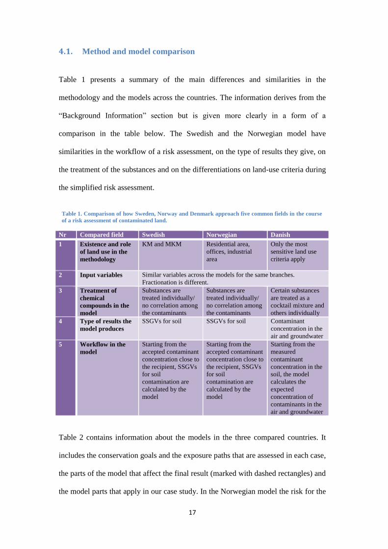
Table 1 presents a summary of the main differences and similarities in the

methodology and the models across the countries. The information derives from the

“Background Information” section but is given more clearly in a form of a

comparison in the table below. The Swedish and the Norwegian model have

similarities in the workflow of a risk assessment, on the type of results they give, on

the treatment of the substances and on the differentiations on land-use criteria during

the simplified risk assessment.

Table 1. Comparison of how Sweden, Norway and Denmark approach five common fields in the course

of a risk assessment of contaminated land.

Nr Compared field Swedish Norwegian Danish

1 Existence and role

of land use in the

methodology

KM and MKM Residential area,

offices, industrial

area

Only the most

sensitive land use

criteria apply

2 Input variables Similar variables across the models for the same branches.

Fractionation is different.

3 Treatment of

chemical

compounds in the

model

Substances are

treated individually/

no correlation among

the contaminants

Substances are

treated individually/

no correlation among

the contaminants

Certain substances

are treated as a

cocktail mixture and

others individually

4 Type of results the

model produces

SSGVs for soil SSGVs for soil Contaminant

concentration in the

air and groundwater

5 Workflow in the

model

Starting from the

accepted contaminant

concentration close to

the recipient, SSGVs

for soil

contamination are

calculated by the

model

Starting from the

accepted contaminant

concentration close to

the recipient, SSGVs

for soil

contamination are

calculated by the

model

Starting from the

measured

contaminant

concentration in the

soil, the model

calculates the

expected

concentration of

contaminants in the

air and groundwater

Table 2 contains information about the models in the three compared countries. It

includes the conservation goals and the exposure paths that are assessed in each case,

the parts of the model that affect the final result (marked with dashed rectangles) and

the model parts that apply in our case study. In the Norwegian model the risk for the

18

environment is qualitatively approached but not addressed by the software. If such a

risk exists, national, general environmental ambitions by the EPA or local

requirements should be met and therefore explicitly investigated

(Miljøverndepartementet 1999).

Table 2. Recipients and exposure paths identified in all the models. The tick sign means that such a value

can be generated by the model while “x” that it cannot. Green cells represent the active parts of the model

in our case study and grey the inactive. The orange rectangles with the dashed outline are the parts of the

software that contribute to the final results. In the Swedish model there are three rectangles instead of one

to show an intermediate calculating step that is absent in the other models. In the Norwegian and in the

Danish model all cells are equally weighed.

Protection goals Exposure paths Swedish Norwegian Danish

Human Soil ingestion x

Skin contact x

Inhalation of soil

particles

x

Inhalation of

vapors

(indoors)

(outdoors)

Consumption of

groundwater

Consumption of

vegetables

x

Consumption of

fish

x

Environment x x

Groundwater x x

Surface water x x

Free phase x

4.2. Case study

4.2.1. Compliance of the field concentrations with the quality criteria and recognition

of most influential paths

The field concentrations exceeded the GGVs in both the Swedish and the Norwegian

model at boreholes SB03, SB05 and SB10. The following advanced risk assessment

generated SSGVs presented in Table 3. For each compound the most influential

pathway/ conservation goal accompanies the SSGV and is shown in the same table.

Despite the different fractionation it is clear that the Swedish model has much lower

SSGVs than the Norwegian model. The Swedish guidelines range from five times

19

lower than the Norwegian in the case of aliphatic hydrocarbons >C8-C10 to up to ten

thousand times more in MtBE.

Table 3. GGVs and SSGVs for the studied petrol station in Sweden and Norway for different chemical

compounds. The concentrations are given in mg of contaminants per kg of soil.

Concerning the most important exposure pathways/ conservation goals in the case

study, the guideline for protection of groundwater has the greatest impact on more

than half of the substances (7/13) in the Swedish model. Protection of environment

comes next by controlling five out of thirteen substances and inhalation of vapors

only one. In the Norwegian model the dominating exposure pathways is the

inhalation of vapors controlling nine out of ten chemical compounds. Soil ingestion

is the most influential pathway in only one substance. The two models coincide in

the identification of the most influential pathway only in aliphatic hydrocarbons

Sweden Norway

Substance SSGV Most

influential

pathway/

conservation

goal

SSGV Most influential

pathway/

conservation goal

Aliphatic hydrocarbons C5-C6 18 Groundwater 406 Inhalation of

vapors

Aliphatic hydrocarbons >C6-C8 120 Groundwater 1,498 Inhalation of

vapors

Aliphatic hydrocarbons >C8-C10 100 Inhalation of

vapors 530

Inhalation of

vapors

Aliphatic hydrocarbons >C10-C12 500 Environment 2,881 Inhalation of

vapors

Aliphatic hydrocarbons >C12-C16 500 Environment - -

Aliphatic hydrocarbons >C16-C35 1,000 Environment - -

Aliphatic hydrocarbons >C12-C35 - - >20,000 Soil ingestion

Aromatic hydrocarbons C8-C10 50 Environment - -

Aromatic hydrocarbons >C10-C16 15 Environment - -

Benzene 0.012 Groundwater 0.66 Inhalation of

vapors

Toluene 15 Groundwater 245 Inhalation of

vapors

Ethylbenzenes 15 Groundwater 906 Inhalation of

vapors

Xylenes 20 Groundwater 812 Inhalation of

vapors

MtBE 0.25 Groundwater 2,588 Inhalation of

vapors

20

>C8-C10 (inhalation of vapors) and have the minimum difference in the issued

guideline.

In Table 4a the SSGV of the Swedish model are compared with the on-site

concentrations. The four samples coming from boreholes SB03, SB05 (both depths)

and SB10 have concentrations of the analyzed parameters in collected soil samples

below the SSGV. The compounds that exceed the values are marked with red and

are:

aliphatic hydrocarbons C5-C6: one sample with double concentration than

SSGV,

aliphatic hydrocarbons >C8-C10: one sample with 11% higher concentration

than SSGV,

aliphatic hydrocarbons >C10-C12: one sample with approximately 10%

concentration over SSGV,

aliphatic hydrocarbons >C12-C16: one sample with higher than double

concentration than the SSGV,

aliphatic hydrocarbons >C16-C35: one sample exceeding the SSGV by 57%,

aromatic hydrocarbons >C10-C16: three samples exceeding the SSGV by 3,

9 and 5 times and

benzene: one sample having approximately 7 times higher concentration than

the SSGV.

In the Norwegian model all analyzed parameters from the collected samples

reported below the SSGVs. Table 4b shows which soil samples (marked with

orange) required further investigation after the simplified risk assessment but

were later on accepted as the risk for human health was acceptable.

21

Samples

Substances SB01/1 SB01/2 SB03/1 SB03/2 SB04/1 SB04/2 SB05/1 SB05/2 SB06/1 SB06/2 SB07/1 SB07/2 SB08/1 SB08/2 SB10/1 SB10/2 SB11/1 SB11/2 SB12/1 SB12/2

Aliphatic hydrocarbons C5-C6 1 1 1.5 1 1 1 1 34.5 1 1 1 1 1 1 10.5 1.5 1 1 1 1

Aliphatic hydrocarbons >C6-C8 1 1 3 1 3.5 1 1 49 1 1 1 1 1 2.5 65 7 1 1 1 1

Aliphatic hydrocarbons >C8-C10 2.5 2.5 79 2.5 2.5 2.5 2.5 134.25 2.5 3.25 2.5 2.5 2.5 4.25 120 14 2.5 2.5 2.5 2.5

Aliphatic hydrocarbons >C10-C12 2.5 2.5 554 2.5 2.5 3.25 2.5 44 2.5 2.5 2.5 33.25 2.5 2.5 90 30 2.5 2.5 2.5 2.5

Aliphatic hydrocarbons >C12-C16 5 5 1155 5 5 35.75 5 282 5 5 5 5 5 5.75 190 20 5 5 5 5

Aliphatic hydrocarbons >C16-C35 10 10 802 10 10 55 32.5 150 69 10 10 32.5 47 10 1577.5 222 10 32.5 10 10

Aromatic hydrocarbons C8-C10 0.80 1.40 6.00 0.80 0.80 0.80 20.00 0.80 0.80 0.80 0.80 0.80 0.80 0.80 7.00 0.80 0.80 0.80 0.80 0.80

Aromatic hydrocarbons >C10-C16 2.00 2.00 62.17 2.00 2.00 2.00 198.67 2.00 2.00 2.00 2.00 2.00 2.00 2.00 88.67 2.00 2.00 2.00 2.00 2.00

Benzene 0.005 0.005 0.005 0.005 0.005 0.005 0.005 0.02 0.005 0.005 0.005 0.005 0.005 0.005 0.1 0.005 0.005 0.005 0.005 0.005

Toluene 0.025 0.025 0.025 0.025 0.025 0.025 0.025 3 0.025 0.025 0.025 0.025 0.025 0.025 0.25 0.025 0.025 0.025 0.025 0.025

Ethylbenzenes 0.025 0.025 0.025 0.025 0.025 0.025 0.025 2 0.025 0.025 0.025 0.025 0.025 0.025 0.025 0.025 0.025 0.025 0.025 0.025

Xylenes 0.05 0.05 0.05 0.05 0.05 0.05 0.05 3.30 0.05 0.05 0.05 0.05 0.05 0.05 0.8 0.05 0.05 0.05 0.05 0.05

MtBE 0.01 0.01 0.01 0.01 0.01 0.01 0.01 0.01 0.01 0.01 0.01 0.01 0.01 0.01 0.01 0.01 0.01 0.01 0.01 0.01

Sweden

Samples

Substances SB01/1 SB01/2 SB03/1 SB03/2 SB04/1 SB04/2 SB05/1 SB05/2 SB06/1 SB06/2 SB07/1 SB07/2 SB08/1 SB08/2 SB10/1 SB10/2 SB11/1 SB11/2 SB12/1 SB12/2

Aliphatic hydrocarbons C5-C6 1 1 1.5 1 1 1 1 34.5 1 1 1 1 1 1 10.5 1.5 1 1 1 1

Aliphatic hydrocarbons >C6-C8 1 1 3 1 3.5 1 1 49 1 1 1 1 1 2.5 65 7 1 1 1 1

Aliphatic hydrocarbons >C8-C10 2.5 2.5 79 2.5 2.5 2.5 2.5 134.25 2.5 3.25 2.5 2.5 2.5 4.25 120 14 2.5 2.5 2.5 2.5

Aliphatic hydrocarbons >C10-C12 2.5 2.5 554 2.5 2.5 3.25 2.5 44 2.5 2.5 2.5 33.25 2.5 2.5 90 30 2.5 2.5 2.5 2.5

Aliphatic hydrocarbons >C12-C35 15 15 1957 15 15 90.75 37.5 432 74 15 15 37.5 52 15.75 1768 242 15 37.5 15 15

Benzene 0.005 0.005 0.005 0.005 0.005 0.005 0.005 0.02 0.005 0.005 0.005 0.005 0.005 0.005 0.1 0.005 0.005 0.005 0.005 0.005

Toluene 0.025 0.025 0.025 0.025 0.025 0.025 0.025 3 0.025 0.025 0.025 0.025 0.025 0.025 0.25 0.025 0.025 0.025 0.025 0.025

Ethylbenzenes 0.025 0.025 0.025 0.025 0.025 0.025 0.025 2 0.025 0.025 0.025 0.025 0.025 0.025 0.025 0.025 0.025 0.025 0.025 0.025

Xylenes 0.05 0.05 0.05 0.05 0.05 0.05 0.05 3.3 0.05 0.05 0.05 0.05 0.05 0.05 0.8 0.05 0.05 0.05 0.05 0.05

MtBE 0.01 0.01 0.01 0.01 0.01 0.01 0.01 0.01 0.01 0.01 0.01 0.01 0.01 0.01 0.01 0.01 0.01 0.01 0.01 0.01

Norway

Table 4. (a) Comparison of the concentration of 13 substances (left side) in 20 different samples with the SSGV generated by the Swedish model. Red cells indicate that the

samples are over both GGVs and SSGVs while the non-highlighted cells mean that they comply with them. (b) Comparison of the concentration of 10 substances with the

GGVs in the Norwegian model. Orange cells are within the fifth CES while the rest concentrations are in lower CES requiring no advanced risk assessment. All the

concentrations comply with the SSGVs in the Norwegian model.

22

In the Danish risk assessment all the samples complied with the GGVs for soil. The

calculated compounds’ concentrations in indoors and outdoors air complied with the

air quality criteria in all boreholes. On the contrary, the estimated groundwater

concentration of the compounds was higher than the drinking norms in every sample.

In Table 5 the results from the groundwater module are presented for three randomly

selected samples: SB03/1, SB05/1 and SB05/2. The TPH concentration in

groundwater is at least 59 times over the limit across the three boreholes, reaching the

highest value in SB05/1. SB05/2 has the highest concentration in aromatic

hydrocarbons which exceed the groundwater criteria by 200 times and has the highest

concentration in toluene. The calculated concentration of MtBE and naphthalene is

over the drinking norms for the three samples. Benzene and fluoranthene

concentration is within the standards whereas toluene exceeds them only in SB05/2.

Table 5. Results of the Danish model for groundwater. The substances presented on the left side are split

into two groups depending on if their soil concentrations are input to the model (first four compounds) or if

they are calculated by the software. The three columns on the right show the ratio of the calculated

groundwater concentration of the substances to the groundwater quality criteria based on the hypothetical

observation data from soil samples SB03/1, SB05/1, SB05/2.

Danish model - Groundwater

Ratio of calculated groundwater concentration to groundwater

criteria

Substance SB03/1

SB05/1 SB05/2

TPH C6 - C35 59.1 83.7 66.6

Benzene 0.014 0.131 0.184

Toluene 0.0094 0.96 3.7

MtBE 6 6 6

Naphthalene 2.7 3 1.5

Fluoranthene 0.39 0.03 0.08

Aromatic hydrocarbons C9 -C10 26.4 65.5 200

23

4.2.2. Analysis of the exposure path of consumption of groundwater

Table 6 presents the calculated pore water and groundwater concentrations based on

the hypothetical observation data from soil sample SB03/1 for benzene, toluene and

MtBE. Quality criteria for groundwater are also presented in the last line for each

compound and they are related to drinking norms. For the Swedish and the Danish

model, the quality criteria have the form of maximum contaminant level (mg/l). The

Norwegian model uses TDI criteria (mg/kg of body weight per day) and therefore

could not be compared with the other two models. For the Swedish and the Danish

model the groundwater concentrations are highlighted with either green or red

depending on if the exceed the maximum contaminant level.

Benzene Swedish Norwegian Danish

Specified concentration in soil (mg/kg) 0.005 0.005 0.005

IGV for groundwater (mg/kg) 0.012 0.0337 -

Calculated pore water concentration (mg/l) 0.0054 0.0054 0.000015

Calculated groundwater concentration (mg/l) 0.0023 0.0015 0.000014

Groundwater criteria (mg/l) 0.0005 - 0.001

Toluene Swedish Norwegian Danish






MtBE Swedish Norwegian Danish






Table 6. Comparison of calculated pore water concentration and groundwater concentration,

groundwater criteria and SSGVs in benzene, toluene and MTBE across the models. The calculations are

based on the hypothetical observation data from soil sample SB03/1. The concentrations in soil and in

groundwater highlighted with green, fulfill the quality criteria or the guidelines while the red ones do not.

24

Additionally, Table 6 shows the IGV for groundwater in the Swedish and the

Norwegian model. When the IGV is higher than the field concentration the sample

complies with the guidelines and the concentration is highlighted with green (first

line). For the Danish model there are no IGVs and the color of highlight depends only

on the groundwater concentration.

For all three substances the soil concentrations are below the SSGVs issued by the

Swedish and the Norwegian model. In the Danish model, benzene and toluene

concentrations are accepted but MtBE has six time higher concentration than the

drinking norms (marked with red). In the case of the Swedish model it is clear that a

compliance with the IGV does not mean that the water quality criteria/ drinking norms

are met; for benzene the calculated groundwater concentration is over the maximum

contaminant level but the soil concentration is still within the guidelines. For toluene

and MtBE both soil and groundwater concentrations comply with the guidelines and

the criteria respectively.

A comparison of the groundwater criteria between the Swedish and the Danish model

shows similar criteria for benzene but considerable differences in toluene and MtBE.

Toluene has 70 times higher acceptable concentration in the Swedish model than in

the Danish model while for MtBE it is 7 times higher.

When it comes to pore- and groundwater concentrations given by the models all three

of them have similar values for MtBE. On the contrary the Danish model gives quite

smaller concentrations for benzene and toluene than the other two models.

25

5. Discussion

The discussion follows the structure of the result section and is consisted of four parts.

First the results of the method and the model comparison are analyzed and then the

case study is on the focus. A discussion of the importance of the results and their

implications on a broader level follows with a brief report to the limitations of the

study.

5.1. Method and model comparison

The Swedish and the Norwegian risk assessment methods for contaminated land show

great similarities. Both countries have a common backbone when they assess the risk

for contaminated land, described by a two-phase risk assessment, use of GGVs,

consideration of land-use, similar fate and transport analysis of the contaminants and a

final generation of SSGVs.

These similarities expand to the models that are used for risk assessment and involve

comparable equations, interfaces and standards (Miljøverndepartementet 1999) in the

calculations.

Overall it can be said that the two countries have very close methods and models to

assess the risk deriving from contaminated areas. This was an expected conclusion

since the Norwegian model is based on an old version of the Swedish one

(Naturvårdsverket 2006).

The Danish risk assessment methodology is more difficult to be compared with the

Swedish and the Norwegian ones for the following reasons.

26

The type of the results given by the models (SSGVs and final

concentration in the vicinity of the recipient) are not comparable.

The inverse calculation path that is followed by the Swedish and

Norwegian model compared to the Danish one.

The cocktail mixture approach in the Danish model that takes into

consideration the interaction between the contaminants while the other

models assume only interaction of the contaminants with the

environment.

The different fractionation of petroleum hydrocarbons both as input to

the model and as output.

Concerning the fractionation of TPH, there is no protocol in Europe. Pinedo (2012)

argues that the fractionation of TPH should be based on their physicochemical

behavior and toxicity and not have a character of TPH as it is in the Danish model.

Peters et al. (1999) suggest to focus on certain petroleum hydrocarbon fractions that

are more dangerous for public health and not use a TPH approach. Park & Park

(2000) are also in favor of using fractions of TPH. For the rest of the differences it

cannot be said that the followed approach from a country is right or wrong as there are

arguments for both sides.

Regardless of the encountered difficulties in the comparison, there are three

conclusions that can be drawn from the theoretical cross-examination of the methods.

1. The Swedish model has the maximum number of recipients generating guideline

values for protection of humans, environment and spreading of the contaminants.

2. The Danish risk assessment is the only one that does not assess ecological risk.

This is in line with the Danish Act on Contaminated Soil (Miljøministeriet 2009)

27

that specifically lists human safety and drinking water as the primary protective

goals from contaminated areas. The Danish EPA has reflected upon the lack of the

ecological risk assessment and has analyzed and compared similar models from

other countries. The study and the comparison of similar models was done to

prepare the ground if the pressure to change the Act on Contaminated Soil

increases from the Water Framework Directive (WFD) and the Habitat Directive

in EU (Miljøstyrelsen 2007 & 2012).

3. Every recipient and exposure path in the models has the same weight in the

calculation of the risk deriving from the contaminated site. For example, the risk

for human health is as important as the risk for the environment in the Swedish

model and all the exposure paths are equated in the Norwegian and the Danish

models. This means that during the use of the models no prioritization according

to paths or recipients takes place.

5.2. Case study

The results of the Swedish and the Norwegian model on the case study are

considerably different. The much lower SSGVs issued by the Swedish model can be

explained by the fact that more exposure paths and recipients are involved into the

calculations than in the Norwegian model. If only the risk for human health was

assessed by the Swedish model, the SSGVs would be higher. This conclusion is

supported by the fact that 12/13 compounds in the Swedish model had the biggest

influence by the exposure paths of spreading of contaminants, and not by the health-

based guideline. When the two models had the same dominating exposure path for a

compound, they had their minimum difference in the SSGVs.

28

The lower SSGVs from the Swedish model resulted to considering the contaminant

concentrations in three boreholes as potentially dangerous for human and/ or the

environment. Thus, further investigation of the site can be considered. While in the

case of the Norwegian model, the site complies with the SSGVs and according to the

available data there is no need for further investigation.

The calculations with the Danish model show a different picture for the contaminated

area with all the samples giving groundwater concentrations over the drinking norms.

This clear exceedance of water quality standards leads to a higher pressure for further

investigation and consideration of remediation than in the case of the Swedish model.

The cross-examination of the module of consumption of groundwater across the

models showed how complicated such a comparison can be. In the first place it

showed that the increased sensitivity of the Danish model cannot be attributed to a

constant overestimation of the concentration of contaminants in the pore-water or in

the groundwater. It also made clear that the disparity in the results is not related to the

drinking norms. The Danish drinking norms for toluene though are remarkably more

demanding than in Sweden. The Danish EPA mentions that toluene’s reference values

are based on the Chemical Abstract Service (Miljøstyrelsen 2014b) while the Swedish

EPA uses values from World Health Organization (Naturvårdsverket 2009a).

Surprisingly enough, the drinking norm for toluene in groundwater from CAS is 1

mg/l (U.S. EPA 2005) which is far greater than the 0.005 mg/l that the Danish EPA

uses. A possible communication with the Danish EPA could clarify this discrepancy.

The overall picture from the comparison of the module of groundwater is that it is

much more conservative in Denmark. Even if this exposure pathway was taken into

consideration in the other two models, the concentrations of the three examined

29

compounds would comply with the groundwater criteria in at least 18 out of 20

samples. Another point that suggests that the Danish model is more conservative than

the other two, is that a calculated concentration of contaminants in the groundwater

over the quality criteria is not accepted in Denmark whereas in the Swedish model it

can still be within the IGV and be accepted (as demonstrated for benzene in SB03/1).

The higher tolerance in the Swedish model is supported by the fact that the drinking

norms concern parts of the water network that support more than 50 people and lead

to consumption of more than 10m3/ day (Livsmedelseverket 2005). Thus not private

use. Moreover, the drinking norms are not legally binding and they serve as a

recommendation to help in deciding if the water is appropriate or not

(Livsmedelsverket 2006).

The increased sensitivity that Denmark shows for groundwater contamination is well

known both inside the country (e.g. Miljøministeriet 2009; Miljøstyrelsen 2012

&2014b) and abroad (e.g. Naturvårdsverket 2006). The Danish EPA wants to guard

the quality of groundwater as it constitutes the main drinking water resource in the

country. The starting point of discussions for protection of groundwater is that after a

simple treatment of the water with aeration and sand filtration, it should meet EU-

Directive’s standards (Miljøstyrelsen 2014b).

5.3. Importance of the results

The demonstrated divergence of the examined risk assessment methods, models and

finally of the results and the conclusions that on the case-study shows how complex it

is to relate contamination on a site with impact to human health and/ or to ecology.

The complexity derives among other reasons from the existence of many direct and

indirect exposure paths (e.g. Abrahams 2002; Chen et al. 2003; Labieniec et al. 1997;

30

MacLeod et al. 2004; Paustenbach 2000) and effects of multiple contaminants on site

(Brouwer et al. 1990; Houk 1992; Park & Park 2010; Powers et al. 2001). Therefore it

has to be further examined how updated such models are with the current state of

knowledge.

In practice, the displayed divergence has major implications. These differences can

affect the decision to remedy a contaminated site and to prioritize remedial action

among contaminated areas (e.g. Miljøstyrelsen 2011). Therefore they show interest

for land-owners, consultants, the countries where the pollution occurs and, last but not

least, the inhabitants that are exposed to risks that are regarded as unacceptable by a

neighboring country.

The land-owners of a polluted site and/ or the countries where the contaminated areas

are, are legally responsible to pay for the land decontamination. In Sweden, about 1

billion SEK per year is spent on land remediation and half of it comes from the

private sector. In Norway, 170 million SEK per year are allocated for the same cause

(Miljøstyrelsen 2012) while in Denmark it was circa 250 million SEK in 2011

(Miljøstyrelsen 2014c).

For consultants who carry out risk assessments for contaminated sites, it is obvious

that the choice of a used method affects the conclusions of a risk assessment.

Companies that are present as a Nordic entity have reflected upon the varying

outcomes of risk assessments and the consequences they bear. The companies want to

efficiently utilize their funding for land decontamination and maximize risk reduction.

Additional implications for the countries from this comparison, involve which

protective goals are in threat by a contaminated site as this affects the priority for

31

remedial action. Norway and Sweden prioritize equally the ecological and human risk

assessment but they allocate more funding in remediation of sites posing risk for

humans (Miljøstyrelsen 2012). Since the models may not recognize the same

recipients being exposed to danger under a risk assessment, the decision that will be

taken may be affected.

Furthermore the risk assessments are used to see if the environmental goals set by the

EPAs on a national level are met or not. In Sweden for example, the goal to have non-

toxic environment (giftfri miljö) will not be met by 2020 (Naturvårdsverket 2014).

But if a different risk assessment methodology was followed the results could maybe

show another picture. On a European level, the same problems exist when countries

report to WFD. As there is no common risk assessment methodology to gauge the

environmental status of countries the results/ reports are not comparable. This

inconsistency creates an uneven basis for discussions about obligations towards the

WFD and will concomitantly impact the need for taken action and the associated legal

implications.

5.4. Potential sources of errors and limitations of the results

The data and the methods used in the thesis may be prone to errors and therefore pose

limitations for the conclusions.

The study of the risk assessment methods and models was mostly based on online

material provided by the EPAs. The information though was usually fragmented in

different documents even when it was issued by the same EPA. Despite the thorough

research and comparison of different sources, it is possible that newer directions or

guidelines may apply and have partially replaced the ones presented here.

32

The case-study was based on fictive data that resembled real case-studies. Thus, the

construction of the examined case study by URS includes subjective choices

regarding the typical presence of the contaminants and the typical geometry and

characteristics of petrol stations. In order to further examine how representative is the

case study and the results and the conclusions that were drawn from it, additional

contaminated sites could be investigated.

The common ground for comparing certain parts of the models was very limited and

this investigation was one of the most time consuming elements of this study. This led

to comparing only one exposure path, for three compounds, in one soil sample which

corresponds to a quite small fragment of the models. Additional examination of other

common features could produce more concrete results.

4. Conclusions

The Swedish and the Norwegian risk assessment methods and models for

contaminated land show great similarities while the Danish one differs on a

conceptual level.

The present case study showed that the differences between the models affect

the results and the conclusions of a risk assessment. The same site can be seen

as posing risk to human health in one country (Denmark), while it complies

with the quality criteria of another country (Norway).

The differences reflect the priorities set by the EPAs when it comes to

protection goals.

The implications of not having a common method and tool to assess the risk

for contaminated land show great interest and mainly affect four groups: Land-

33

owners who may be called to cover the decontamination expenses. Consultants

and companies who perform risk assessments and land remediation. The

countries that have to meet national and international environmental goals and

can also share/ or cover the cost for decontamination. The people who are

exposed an environment seen as potential harmful by a neighboring country.

Although robust conclusions were obtained for the considered case, the fact

that realistic but hypothetical input data was used in the case study means that

future studies would need to further address questions regarding how frequent

and pronounced such diverging results are.

34

5. References

Abrahams, P.W., 2002, ‘Soils: Their implications to human health’, The Science of

the Total Environment, vol. 291, issue 1-3, p. 1-32, doi: 10.1016/S0048-

9697(01)01102-0.

Brouwer, A., Murk, A.J., Koeman, J.H., 1990, ‘Biochemical and physiological

approaches in ecotoxicology’, Functional Ecology, vol. 4, issue 3, p. 275-281, doi:

10.2307/2389586.

Chen, Z., Huang, G.H., Chakma, A., 2003, ‘Hybrid fuzzy-stochastic modeling

approach for assessing environmental risks of contaminated groundwater systems’,

Journal of Environmental Engineering – ASCE, vol. 129, issue 1, p. 79-88, doi:

10.1061/(ASCE)0733-9372(2003)129:1(79).

Cushman, D.J., Driver, K.S., Ball, S.D., 2001. ‘Risk assessment for environmental

contamination: an overview of the fundamentals and application of risk assessment

at contaminated sites’. Canadian Journal of Civil Engineering 28[1], 155-162.

NRC Research Press. doi: 10.1139/cjce-28-S1-155.

European Commission 2012, Guidance on the interpretation of key provisions of

Directive 2008/98/EC on waste, Directorate-General Environment.

European Commission 2014 – Joint Research Centre (JRC), Progress in the

management of Contaminated Sites in Europe, Institute for Environment and

Sustainability, doi: 10.2788/4658.

Ferguson, C., Darmendrail, D., Freier, K., Jensen, B.K., Jensen, J., Kasamas, H.,

Urzelai, A. and Vegter, J. 1998, ‘Risk Assessment for Contaminated Sites in

Europe’. Scientific Basis. Vol. 1. LQM Press, Nottingham.

Guyonnet, D., Bourgine, B., Dubois, D., Fargier, H., Côme, B., Chilès, J., 2003,

‘Hybrid Approach for addressing Uncertainty in Risk Assessments’, Journal of

35

Environmental Engineering-ASCE, vol. 129, issue 1, p. 68-78, doi:

10.1061/(ASCE)0733-9372(2003)129:1(68).

Houk, V.S., 1992, ‘The genotoxicity of industrial wastes and effluents’, Mutation

Research, vol. 277, issue 2, p. 91-138, doi: 10.1016/0165-1110(92)90001-P.

Labieniec, P.A., Dzombak, D.A., Siegrist, R.L., 1997, ‘Evaluation of uncertainty in

site-specific risk assessment’, Journal of Environmental Engineering –ASCE, vol.

123, Issue 3, p. 234-243, doi: 10.1061/(ASCE)0733-9372(1997)123:3(234).

Li Jianbing, Huang H. Gordon, Zeng Guangming, Maqsood Imran, Huang Yuefei,

2007, ‘An integrated fuzzy-stochastic modeling approach for risk assessment of

groundwater contamination’, Journal of Environmental Management, vol. 82, issue

2, p. 173-188, doi: 10.1016/j.jenvman.2005.12.018.

Linkov, I., Loney, D., Cormier, S., Satterstrom, F.K., Bridges, T., 2009, ‘Weight-of-

evidence evaluation in environmental assessment: Review of qualitative and

quantitative approaches’, Sciences of the Total Environment, vol. 407, issue 19, p.

5199-5205, doi: 10.1016/j.scitotenv.2009.05.004.

Livsmedelsverket – Swedish National Food Agency 2006, Vägledning till

Livsmedelsverkets föreskrifter om dricksvatten (SLVFS 2001:30) [Guidance for

Swedish National Food Agency’s regulations for drinking water (SLVFS 2001:30)]

(In Swedish), Tillsynsavdelningen, Enheten för inspektion.

MacLeod, M., McKone, T.E., Foster, K.L., Maddalena, R.L., Parkerton, T.F.,

MacKay, D., 2004, ‘Applications of Contaminants and Bioaccumulation Models in

Assessing Ecological Risks of Chemicals: A Case Study for Gasoline

Hydrocarbons’, Environmental Science & Technology. vol 38, p. 6225-6233. doi:

10.1021/es049752+.

Miljøministeriet - Danish Ministry of the Environment 2009, Bekendtgørelse af lov

om forurenet jord LBK nr 1427 af 04/12/2009 [Act on Contaminated Soil (No. 1427

of 2009)] (In Danish).

36

Miljøstyrelsen - Danish Environmental Protection Agency 2002, Guidelines on

remediation of contaminated sites, Environmental guidelines no 7.

Miljøstyrelsen - Danish Environmental Protection Agency 2007, Consolidating

Regulation 22-03-2007 No. 282 on Contaminated Soil, LBKG2007282.

Miljøstyrelsen - Danish Environmental Protection Agency 2011, Værktøjer til brug

for risikovurdering og prioritering af grundvandstruende forureninger [Tool for

risk evaluation and prioritization of threat for groundwater pollution] (In Danish),

Environmental Project 1366 2011, Teknologiprogrammet for jord- og

grundvandsforurening.

Miljøstyrelsen - Danish Environmental Protection Agency 2012, Ecological risk

assessment of contaminated sites, Environmental project 1422.

Miljøstyrelsen - Danish Environmental Protection Agency 2013, Manual for program

til risikovurdering –JAGG 2.0 (in Danish), Environmental project 1508.

Miljøstyrelsen - Danish Environmental Protection Agency 2014a, Bilag til

redegørelse om jordforurening 2011, [Appendix of remediation of contaminated

land 2011] (in Danish).

Miljøstyrelsen - Danish Environmental Protection Agency 2014b, Liste over

kvalitetskriterier i relation til forurenet jord og kvalitetskriterier for drikkevand,

[List of quality criteria concerning contaminated soil and quality criteria for

drinking water] (in Danish).

Miljøstyrelsen - Danish Environmental Protection Agency 2014c, Redegørelse om

Jordforurening 2011 [Statement in soil pollution 2011] (In Danish).

Miljøverndepartementet – Norwegian Environmental Protection Agency 1999,

Veiledning om risikovurdering av forurenset grunn [Directions for risk evaluation

of polluted wells] (In Norwegian). Norwegian Pollution Control Authority.

Guidance 99:01a.

37

Miljøverndepartementet – Norwegian Environmental Protection Agency 2009,

Helsebaserte tilstandsklasser for forurenset grunn [Health based classes of

environmental state for polluted wells] (In Norwegian). Norwegian Pollution

Control Authority. Guidance TA-2553.

Naturvårdsverket – Swedish Environmental Protection Agency 2002, Methods for

inventories of Contaminated Sites.

Naturvårdsverket – Swedish Environmental Protection Agency 2006, Fördjupade

riskbedömningar. Erfarenheter av riktvärdesberäkningar och användning av ny

kunskap [Advanced risk assessments. Experiences from generation of guideline

values and use of gained knowledge] (In Swedish). Report 5592.

Naturvårdsverket – Swedish Environmental Protection Agency 2009a, Riktvärden för

förorenad mark [Guideline values for contaminated soil] (In Swedish). Report

5976.

Naturvårdsverket – Swedish Environmental Protection Agency 2009b,

Riskbedömning av förorenade områden [Risk assessment for contaminated sites]

(In Swedish). Report 5977.

Naturvårdsverket – Swedish Environmental Protection Agency 2014, Miljömålen

Årlig uppföljning av Sveriges miljökvalitetsmål och etappmål 2014 [Environmental

goals Annual follow-up of Swedish environmental quality and interim goals] (in

Swedish). Report 6608.

NICOLE, Network for Industrially Contaminated Land in Europe, 2004, Risk

Assessment Comparison Study, NICOLE Project, Appendix F Part 1.

Park, In-Sun, Park, Jae-Woo, 2000, ‘A novel total petroleum hydrocarbon

fractionation strategy for human health risk assessment for petroleum hydrocarbon-

contaminated site management’, Journal of Hazardous Materials, vol. 179, issue 1-

3, p. 1128-1135, doi: 10.1016/j.jhazmat.2010.03.124.

38

Paustenbach, D.J., 2000, ‘The practice of exposure assessment: A state-of-the-art

review’, Journal of Toxicology and Environmental Health, Part B: Critical

Reviews, 3:3, p. 179-291, doi: 10.1080/10937400050045264.

Peters, C.A., Knightes, C.D., Brown, D.G., 1999, ‘Long-Term Composition

Dynamics of PAH-Containing NAPLs and Implications for Risk Assessment’,

Environmental Science & Technology, vol. 33, issue 24, p. 4499-4507, doi:

10.1021/es981203e.

Powers, S.E., Hunt, C.S., Heermann, S.E., Corseuil, H.X., Rice, D., Alvarez, P.J.J.,

2001, ‘The Transport and Fate of Ethanol and BTEX in Groundwater

Contaminated by Gasohol’, Critical Reviews in Environmental Science and

Technology, Vol. 31, Issue 1, p. 79-123. Doi: 10.1080/20016491089181.

Pinedo, J., Ibanez, R. Prima, O. and Irabien Gulias, A., 2012, ‘Hydrocarbons Analysis

for Risk Assessment in Polluted Soils’, Chemical Engineering Transactions, The

Italian Association of Chemical Engineering, Vol. 28, p. 79-84. doi:

10.3303/CET1228014.

Suter II, G.W., 2006, Ecological Risk Assessment. CRC Press, Boca Raton, USA.

Thompson, K.M., Burmaster, D.E., Crouch, E.A.C., 1992, ‘Monte Carlo Techniques

for Quantitative Uncertainty Analysis in Public Health Risk Assessments’, Risk

Analysis, vol. 12, issue 1, p. 53-63, doi: 10.1111/j.1539-6924.1992.tb01307.x.

Troldborg, M., 2010, Risk assessment models and uncertainty estimation of

groundwater contamination from point sources, PhD thesis, Technical University

of Denmark.

U.S. EPA - United States Environmental Protection Agency, 2005, Toxicological

review of toluene. CAS No. 108-88-3.

Van Straalen, N.M., 2002, ‘Assessment of soil contamination’, Biodegradation, vol.

13, issue 1, p. 41-52, doi: 10.1023/A:1016398018140.

39

6. Appendix

Fig. 1. Map of the hypothetical petrol station. The location of the boreholes is designated with black circles

accompanied by the code of the bore sample. The outline of the buildings is marked with grey.

40

Table 1. Chemical analysis from the soil samples at the petrol station. The lab results refer to the concentration of 72 compounds in soil (left side) at ten boreholes (SB01-SB12). Each

borehole has two samples at different depths e.g. SB01/1 and SB01/2 for borehole SB01. Concentrations are given in mg/kg dry weight soil.

Sample SB01/01 SB01/02 SB03/01 SB03/02 SB04/01 SB04/02 SB05/01 SB05/02 SB06/01 SB06/02 SB07/01 SB07/02 SB08/01 SB08/02 SB10/01 SB10/02 SB11/01 SB11/02 SB12/01 SB12/02

SubstanceLimit of Depth (m)

detection (mg/kg) 2 5 0.7 4.2 0.8 3.2 1.5 3 0.8 2 1.5 2.8 1 2.5 1 4 1.5 3 2 4.2

Aliphatic hydrocarbons C5 1 0.5 0.5 0.5 0.5 0.5 0.5 0.5 0.5 0.5 0.5 0.5 0.5 0.5 0.5 0.5 0.5 0.5 0.5 0.5 0.5

Aliphatic hydrocarbons C6 1 0.5 0.5 1 0.5 0.5 0.5 0.5 34 0.5 0.5 0.5 0.5 0.5 0.5 10 1 0.5 0.5 0.5 0.5

Aliphatic hydrocarbons C7 1 0.5 0.5 1 0.5 3 0.5 0.5 44 0.5 0.5 0.5 0.5 0.5 2 15 2 0.5 0.5 0.5 0.5


Aliphatic hydrocarbons C9 2.5 1.25 1.25 43 1.25 1.25 1.25 1.25 133 1.25 2 1.25 1.25 1.25 3 50 6 1.25 1.25 1.25 1.25

Aliphatic hydrocarbons C10 2.5 1.25 1.25 36 1.25 1.25 1.25 1.25 1.25 1.25 1.25 1.25 1.25 1.25 1.25 70 8 1.25 1.25 1.25 1.25

Aliphatic hydrocarbons C11 2.5 1.25 1.25 7 1.25 1.25 1.25 1.25 21 1.25 1.25 1.25 32 1.25 1.25 60 10 1.25 1.25 1.25 1.25

Aliphatic hydrocarbons C12 2.5 1.25 1.25 547 1.25 1.25 2 1.25 23 1.25 1.25 1.25 1.25 1.25 1.25 30 20 1.25 1.25 1.25 1.25

Aliphatic hydrocarbons C13 2.5 1.25 1.25 547 1.25 1.25 1.25 1.25 23 1.25 1.25 1.25 1.25 1.25 1.25 20 5 1.25 1.25 1.25 1.25

Aliphatic hydrocarbons C14 2.5 1.25 1.25 568 1.25 1.25 32 1.25 2 1.25 1.25 1.25 1.25 1.25 2 50 8 1.25 1.25 1.25 1.25




Aliphatic hydrocarbons C18 1 0.5 0.5 0.5 0.5 0.5 0.5 0.5 0.5 4 0.5 0.5 0.5 0.5 0.5 700 100 0.5 0.5 0.5 0.5

Aliphatic hydrocarbons C19 1 0.5 0.5 0.5 0.5 0.5 0.5 0.5 0.5 0.5 0.5 0.5 0.5 0.5 0.5 200 50 0.5 0.5 0.5 0.5

Aliphatic hydrocarbons C20 1 0.5 0.5 0.5 0.5 0.5 0.5 0.5 0.5 0.5 0.5 0.5 23 0.5 0.5 100 20 0.5 0.5 0.5 0.5

Aliphatic hydrocarbons C21 1 0.5 0.5 3 0.5 0.5 0.5 0.5 0.5 0.5 0.5 0.5 0.5 0.5 0.5 50 30 0.5 0.5 0.5 0.5


Aliphatic hydrocarbons C23 1 0.5 0.5 3 0.5 0.5 23 0.5 0.5 0.5 0.5 0.5 0.5 0.5 0.5 1 0.5 0.5 0.5 0.5 0.5

Aliphatic hydrocarbons C24 1 0.5 0.5 2 0.5 0.5 0.5 0.5 0.5 0.5 0.5 0.5 0.5 0.5 0.5 0.5 0.5 0.5 0.5 0.5 0.5

Aliphatic hydrocarbons C25 1 0.5 0.5 2 0.5 0.5 0.5 0.5 4 0.5 0.5 0.5 0.5 0.5 0.5 0.5 0.5 0.5 0.5 0.5 0.5



Aliphatic hydrocarbons C27 1 0.5 0.5 2 0.5 0.5 0.5 0.5 34 56 0.5 0.5 0.5 0.5 0.5 0.5 0.5 0.5 0.5 0.5 0.5

Aliphatic hydrocarbons C28 1 0.5 0.5 0.5 0.5 0.5 0.5 0.5 34 0.5 0.5 0.5 0.5 0.5 0.5 0.5 0.5 0.5 0.5 0.5 0.5

Aliphatic hydrocarbons C29 1 0.5 0.5 3 0.5 0.5 23 0.5 0.5 0.5 0.5 0.5 0.5 0.5 0.5 0.5 0.5 0.5 0.5 0.5 0.5


Aliphatic hydrocarbons C31 1 0.5 0.5 46 0.5 0.5 0.5 0.5 34 0.5 0.5 0.5 0.5 34 0.5 0.5 0.5 0.5 23 0.5 0.5


Aliphatic hydrocarbons C33 1 0.5 0.5 0.5 0.5 0.5 0.5 23 0.5 0.5 0.5 0.5 0.5 4 0.5 0.5 0.5 0.5 0.5 0.5 0.5


Aliphatic hydrocarbons C35 1 0.5 0.5 0.5 0.5 0.5 0.5 0.5 0.5 0.5 0.5 0.5 0.5 0.5 0.5 0.5 0.5 0.5 0.5 0.5 0.5

Aromatic hydrocarbons C5 0 0 0 0 0 0 0 0 0 0 0 0 0 0 0 0 0 0 0 0 0




Aromatic hydrocarbons C9 0.4 0.40 1.00 4.00 0.40 0.40 0.40 10.00 0.40 0.40 0.40 0.40 0.40 0.40 0.40 2.00 0.40 0.40 0.40 0.40 0.40


41







Aromatic hydrocarbons C17 4 0.1 0.1 0.1 0.1 0.1 0.1 0.1 0.1 0.1 0.1 0.1 0.1 0.1 0.1 0.1 0.1 0.1 0.1 0.1 0.1




















Bensen 0.01 0.005 0.005 0.005 0.005 0.005 0.005 0.005 0.02 0.005 0.005 0.005 0.005 0.005 0.005 0.1 0.005 0.005 0.005 0.005 0.005

Toluene 0.05 0.025 0.025 0.025 0.025 0.025 0.025 0.025 3 0.025 0.025 0.025 0.025 0.025 0.025 0.25 0.025 0.025 0.025 0.025 0.025

Etylbensen 0.05 0.025 0.025 0.025 0.025 0.025 0.025 0.025 2 0.025 0.025 0.025 0.025 0.025 0.025 0.025 0.025 0.025 0.025 0.025 0.025

m-Xylen 0.025 0.0125 0.0125 0.0125 0.0125 0.0125 0.0125 0.0125 0.3 0.0125 0.0125 0.0125 0.0125 0.0125 0.0125 0.1 0.0125 0.0125 0.0125 0.0125 0.0125

o-Xylen 0.025 0.0125 0.0125 0.0125 0.0125 0.0125 0.0125 0.0125 2 0.0125 0.0125 0.0125 0.0125 0.0125 0.0125 0.2 0.0125 0.0125 0.0125 0.0125 0.0125

p-Xylen 0.05 0.025 0.025 0.025 0.025 0.025 0.025 0.025 1 0.025 0.025 0.025 0.025 0.025 0.025 0.5 0.025 0.025 0.025 0.025 0.025

Xylener 0.1 0.05 0.05 0.05 0.05 0.05 0.05 0.05 3.3 0.05 0.05 0.05 0.05 0.05 0.05 0.8 0.05 0.05 0.05 0.05 0.05

MtBE 0.02 0.01 0.01 0.01 0.01 0.01 0.01 0.01 0.01 0.01 0.01 0.01 0.01 0.01 0.01 0.01 0.01 0.01 0.01 0.01 0.01

42

Table 2. Configuration and report of the Swedish model

Konceptuell förorenings- och spridningsmodell Naturvårdsverket, version 1.00

Eget scenario: MKM Gas station

Generellt scenario: MKM

Frigörelse-/

Föroreningskällor spridningsmekanismer Exponeringsvägar

Ytlig mark- Utlakning till Hudkontakt Människor Miljö Naturresurser

förorening grundvatten och jord

ytvatten

Djupt liggande Intag av jord

markförorening Spridning via Boende på platsen: Mark- Grundvatten

grundvatten -Vuxna ekosystem

Inandning -Barn

Markförorening damm

under grund- Spridning via

vattenyta ytvatten Regelbundet verk-

Inandning av samma på platsen:

ånga från jord -Vuxna

Förorening Förångning -Barn Ytvatten- Ytvatten

i grundvatten ekosystem

Intag av dricks-

Vinderosion vatten Besökande:

Förorening -Vuxna

i sediment -Barn

Vattenerosion, Intag av frukt,

ras och skred bär, svamp,

Förorening rot- & grönsaker Närboende:

som fri fas -Vuxna Sediment- Övrigt

Frifasspridning -Barn ekosystem

Intag av fisk

Förorening finns

i/omkring: Upptag i växter Övrigt

-Lagringstankar Bevattning

-Rörledningar

-Avfall/deponi Övrigt

-Ledningsgravar Intag av mjölk,

-Övrigt kött och ägg Övrigt

Hudkontakt

Pågående med sediment

verksamhet

Övrigt

Övrigt

Skyddsobjekt

I detta blad kan en konceptuell förorenings- och spridningsmodell utarbetas för ett objekt.

Vägledning för hur denna tas fram finns i Naturvårdsverkets rapport Riskbedömning av

förorenade områden (rapport 5977), se www.naturvardsverket.se/ebh. Avsikten är att initialt

göra en kvalitativ bedömning av vilka föroreningskällor, frigörelsemekanismer, spridningsvägar,

möjliga exponeringsvägar och skyddsobjekt som är aktuella och behöver beaktas i projektet. En

del av exponeringsvägarna kan beräkningsprogrammet hantera (röd text nedan). Risker kopplade

till andra exponeringsvägar måste hanteras utanför programmet. Den konceptuella modellen kan

användas som underlag vid diskussioner mellan olika parter i projektet.

Återställ formulär

43

Indata för beräkning av riktvärden Naturvårdsverket, version 1.00

Scenariots namn: MKM Gas station Hämta generellt scenario:

Hämta eget scenario:

MKM

Exponeringstid barn 60 60 dag/år

Exponeringstid vuxna 200 200 dag/år




MKM Exponeringstid vuxna 200 200 dag/år

Andel inomhusvistelse 1 1 -



Andel inomhusvistelse 1 1 -

Konsumtion, barn 0 0 kg/dag

Konsumtion, vuxna 0 0 kg/dag

Andel från odling på plats 0 0 -

MKM

Halt löst/mobilt organiskt kol 0.000003 0.000003 kg/dm3 MKM

Torrdensitet 1.7 1.5 kg/dm3 Områdets längd 40 50 m

Halt organiskt kol 0.01 0.02 kg/kg Områdets bredd 19 50 m

Vattenhalt 0.3 0.32 dm3/dm3

Andel porluft 0.1 0.08 dm3/dm3

Total porositet 0.4 dm3/dm3 Mäktighet under gv-ytan 1 m

Standardscenario för mindre känslig markanvändning, enligt

Naturvårdsverkets generella riktvärden för förorenad mark.Val av eget scenario (data till vita inmatningsceller)

Val av generellt scenario (gulbruna celler)

Val av ämnen

Ämne 1:

Ämne 2:

Ämne 3:

Ämne 4:

Ämne 5:

Ämne 6:

Ämne 7:

Ämne 8:

Ämne 9:

Ämne 10:

Ämne 11:

Ämne 12:

Ämne 13:

Ämne 14:

Ämne 15:

Ämne 16:

Ämne 17:

Ämne 18:

Ämne 19:

Ämne 20:

Ämne 21:

Ämne 22:

Ämne 23:

Ämne 24:

Jord- och grundvattenparametrar

Förorenat område

Val av exponeringsvägar

Intag av förorenad jord

Hudkontakt med jord/damm

Inandning av damm

Inandning av ånga

Intag av växter

Beskrivning av scenariot

Beskrivning:

Scenariospecifika modellparametrar

Exponeringsparametrar

Riktvärdet avser endast jord under

Intag av jord

Hudkontakt med jord/damm

Inandning av damm

Inandning av ånga

Intag av dricksvatten

Intag av växter

Uppskattning av halt i fisk

grundvattenytan

Använd KM-värden i modellen

Använd MKM-värden i modellen

44

MKM MKM

Luftvolym inne i byggnad 380 240 m3 Grundvattenbildning 100 100 mm/år

Luftomsättning i byggnad 12 12 1/dag Hydraulisk konduktivitet 5.00E-05 1.00E-05 m/s

Yta under byggnad 160 100 m2 Hydraulisk gradient 0.001 0.03 m/m

Djup till förorening 1.1 0.35 m Akviferens mäktighet 10 10 m

Utspädning till inomhusluft 17338 Avstånd till brunn 200 200 m

Utspädning till utomhusluft 3744324 Utspädning till grundv. (brunn) 29 ggr

MKM MKM

6000 ~6000 ggr

600000 ~600000 ggr

47 47 ggr

Sjöns volym 1000000 1000000 m3 4000 4000 ggr

Sjöns omsättningstid 1 1 år

Flöde i rinnande vattendrag 0.03171 0.03171 m3/s

Modellens utspädning 13158 ggr Flöde genom föroren. massor 76.0 m3/år

Flöde genom akviferen 299.6 m3/år

MKM

MKM

MKM MKM

Avstånd till skyddat gv 200 200 m

Egen utspädningsfaktor 47 47 ggr

Utspädning till skyddat gv 29 ggr

MKM Gas station

0

7.6 m3/dag

7.6 m3/dag

Arsenik-mod

Transportmodeller - Egna utspädningsfaktorer

Transportmodell - Ånga till inom- och utomhusluft

Transportmodell - Ytvatten

Sjö

Rinnande vattendrag

Skydd av markmiljö

Skydd av grundvatten samt justeringar

Använd KM-värden i ämnesdatabas

Använd MKM-värden i ämnesdatabas

Skapa ämne

Ta bort ämne

Skapa, ta bort eller ändra eget ämne

Spara ändring

Ändra modellparameter

Spara ändring

Transportmodell - Grundvatten

Porluft till inomhusluft

Porluft till utomhusluft

Porvatten till grundv. (brunn)

Porvatten till ytvatten

Markmiljö beaktas i sammanvägning hälsa/miljö

Justering för aktuttoxicitet

Justering för bakgrundshalt

Skydd av grundvatten beaktas Egen utspädningsfaktor

Skydd av grundvatten - Utspädning:

Lägg till, spara eller ta bort scenario

Ta bort scenario

Lägg till nytt/sparascenarioÄndra scenariots namn längst upp på

bladet (cell C4).

Välj scenario som ska tas bort:

Skapa eget ämne från befintligt:

Ange namn på eget ämne:

Välj eget ämne som ska tas bort:

Välj eget ämne som ska ändras:

Välj ämnesparameter:

Redigera ämnesparameter:

Välj modellparameter:

Standardvärde:

Redigera modellparameter:

Scenariots namn:

Transportmodeller - Beräknade vattenflöden

Återställ alla

Referens:

Spara referens

Nollställ referenseRedigera referens:

45

Uttagsrapport Eget scenario: MKM Gas station Naturvårdsverket, version 1.00

Generellt scenario: MKM

Beräknade riktvärden

Ämne Riktvärde Styrande för riktvärde Kommentarer (obl = obligatorisk, frv = frivillig)

Alifat >C5-C6 18 mg/kg Skydd av grundvatten

Alifat >C6-C8 120 mg/kg Skydd av grundvatten

Alifat >C8-C10 100 mg/kg Inandning ånga + exp. andra källor

Alifat >C10-C12 500 mg/kg Skydd av markmiljö

Alifat >C12-C16 500 mg/kg Skydd av markmiljö

Alifat >C16-C35 1,000 mg/kg Skydd av markmiljö

Aromat >C8-C10 50 mg/kg Skydd av markmiljö

Aromat >C10-C16 15 mg/kg Skydd av markmiljö

Bensen 0.012 mg/kg Skydd av grundvatten

Toluen 15 mg/kg Skydd av grundvatten

Etylbensen 15 mg/kg Skydd av grundvatten

Xylen 20 mg/kg Skydd av grundvatten

MTBE 0.25 mg/kg Skydd av grundvatten

Avvikelser i scenarioparametrar Eget scenario Generellt scenario

MKM Gas station MKM

Torrdensitet 1.7 1.5 kg/dm3 Fill, sand and gravel (obl)

Halt organiskt kol 0.01 0.02 kg/kg Same preset value in the Norwegian model (obl)

Vattenhalt 0.3 0.32 dm3/dm3 Characteristics for fill material (obl)

Andel porluft 0.1 0.08 dm3/dm3 Characteristics for fill material (obl)

Längd på förorenat område 40 50 m Dimensions of the polluted area according to GGM (obl)

Bredd på förorenat område 19 50 m Dimensions of the polluted area according to GGM (obl)

Luftvolym inne i byggnad 380 240 m3 Based on the map and logical assumptions for building

height (obl)

Yta under byggnad 160 100 m2 Measured on the site map (obl)

Djup till förorening 1.1 0.35 m Average depth from all the boreholes (obl)

Hydraulisk konduktivitet 0.00005 0.00001 m/s Field data (obl)

Hydraulisk gradient 0.001 0.03 m/m Field data (obl)

Avvikelser i modellparametrar Eget värde Standardvärde

Inga avvikelser i modellparametrar. - -

Egendefinierade ämnen

Inga egendefinierade ämnen används.

Standardscenario för mindre känslig markanvändning, enligt Naturvårdsverkets

generella riktvärden för förorenad mark.

Beskrivning

46

Table 3. Configuration of the Norwegian model.

Tabell I. Eksponeringsveier ved aktuell arealbruk. (Kun verdier i gull felt kan endres. Endringer skal begrunnes.)

Parametre Standard

verdi

Anvendt

verdi

Enhet Begrunnelse

(Gule celler må fylles)

365 60 dager/år

8 8 timer/dag

365 200 dager/år

8 8 timer/dag

80 60 dager/år

8 8 timer/dag

45 90 dager/år

8 8 timer/dag

365 60 dager/år

24 8 timer/dag

365 200 dager/år

24 8 timer/dag

365 60 dager/år

24 8 timer/dag

365 200 dager/år

24 8 timer/dag

100% 0% UAKTUELL Exposure pathway not included in the CSM



Parametre Symbol Standard

verdi

Anvendt

verdi

Enhet Begrunnelse

(Gule celler må fylles)

Jordspesifikke data

Vanninnhold i jord qw 0.2 0.3 l vann/l jord Based on fill material characteristics

Luftinnhold i jord qa 0.2 0.1 l luft/l jord Based on fill material characteristics

Jordas tetthet rs 1.7 1.7 kg/l jord

Fraksjon organisk karbon i jord foc 1% 1%

Jorda porøsitet e 40% 40%

Parametre brukt til beregning av konsentrasjon i innedørsluft

Innvendig volum av huset Vhus 240 380 m3 Based on the map and logical assumptions for building height

Areal under huset A 100 160 m2 Measured on the site map

Utskiftingshastighet for luft i huset l 12 12 d-1

Innlekkingshastighet av poreluft L 2.4 2.4 m3/d

Dybde fra kjellergulv til forurensning Z 0.35 1.1 m Average depth from all the boreholes

Diffusiviteten i ren luft Do 0.7 0.7 m2/d

Data brukt til beregning av konsentrasjon i grunnvann

Jordas hydraulisk konduktivitet 0.00001 0.00005 m/s

k 315.36 1576.8 m/år

Avstand til brønn X 0 0 m

Lengden av det forurensende området i

gunnvannsstrømmens retningLgw 50 40 m

Dimensions of the polluted area according to GGM

Infiltrasjons faktor IF 0.141 0.141 år/m

Gjennomsnittlig årlig nedbørmengde P 730 500 mm/år Average value for the three compared countries

Infiltrasjonshastigheten I 0.1 0.1 m/år Beregnet (IF • P2)

Hydraulisk gradient i 0.03 0.001 m/m Field data

Tykkelsen av akviferen da 5 10 m Same preset value in the Swedish model

Tykkelsen av blandingssonen i akviferen dmix 5 6.473789 m Beregnet (ligning (10) i SFT 99:01a)

Data brukt til beregning av konsentrasjon i overflatevann

Vannføring i overflatevann Qsw 500000 1000000 m3/år Same value as in the Swedish model

Bredden av det forurensende området vinkel-

rett på retningen av grunnvannsstrømmenLSW 7.34 19 m

Dimensions of the polluted area according to GGM

Beregnet hastighet på grunnvannstrøming Qdi 347.21136 193.9495 m3/år Beregnet (k • i • dmix • LSW)

Eksponeringstid for oralt inntak av jord (barn)

Same as in the Swedish model




Oppholdstid utendørs (barn)

Fraksjon av inntak av grønnsaker dyrket på lokaliteten

Oppholdstid innendørs (barn)

Eksponeringstid for oralt inntak av jord (voksne) Same as in the Swedish model

Oppholdstid innendørs (voksne)

Tabell II. Transport og reaksjonsmekanismer (tabell 21 s.99 i SFT 99:01A; Kun verdier i gule felt kan endres. Endringer skal begrunnes.)

Fraksjon av inntak av fisk fra nærliggende resipient

Field data

Same as in the Swedish modelOppholdstid utendørs (voksne)

Fraksjon av grunnvann fra lokaliteten brukt som

Eksponeringstid for hudkontakt med jord (barn)

Eksponeringstid for hudkontakt med jord (voksne)



47

Table 4. Configuration and report from the Danish model.

Oliestoffer - fugacitetsberegningerLokalitetenNavn: Lokalitetsnr.:

Adresse: Postnr/by:

Matrikel nr.: Projekt nr.:

Note

JordKommentar Standard data Indtastede data (angives med fed)

Jordtype

Poreluftvolumen VL

Vand-indhold VV

Samlet porøsitet e=VL+VV

Volumen af jordskellet VJ

Kornrumvægt d

Volumenvægt r

Indhold af organisk kulstof foc

Beregning: Fugacitet

Kommentar

Ind

taste

de

væ

rdie

r

Be

reg

ne

t u

d fra

pro

fil

Ind

taste

de

væ

rdie

r

Ove

rskri

de

lse

af kri

teri

et

Be

reg

ne

t u

d fra

fug

acite

t

Gru

nd

va

nd

s-

kri

teri

et

Ove

rskri

de

lse

af kri

teri

et

Be

reg

ne

t u

d fra

fug

acite

t

Afd

am

pn

ing

s-

kri

teri

et

Ove

rskri

de

lse

af kri

teri

et

mg/kg mg/kg mg/kg gange µg/l µg/l gange mg/m³ mg/m³ gange

BTEX'er

Benzen 0.005 0.005 1.5 Nej 0.0146 1 Nej 1.0247 1.3E-04 7,883

Toluen 0.025 0.025 0.0482 5 Nej 1.4241 0.4 3.5603

Ethylbenzen 0.025 0.025 0.0338 0.4475

Sum Xylener 0.005 0.005 0.0066 5 Nej 0.0764 0.1 5.2389

Naphtalen 5.1181 2.7797 1 2.7797 0.5579 0.04 13.947

Kulbrintefraktioner

C6-C10 89 89 25 3.56 31.921 4,499

C10-C15 1,735 1,735 509 156

C15-C20 462 462 0.6399 1.007

C20-C35 377 377 0.0308 1.2E-04

Sum af kulbrinter 2,664 2,664 100 26.64 542 9 60.266 4,667 0.1 46,666

Alkylbenzener

C9-C10 aromatiske kulbrinter 26.622 1 26.9 68.311 0.03 2,319

Polyaromatiske Kulbrinter (PAH)

Benzo(a)pyren 0.15 0.3 Nej 7.4E-05 0.01 Nej 3.9E-10

benzo(b+j+k)fluoranthen 0.3 1.4E-04 3.6E-10

benzo(ghi)perylen 0.15 1.1E-05 5.1E-12

Dibenz(a,h)anthracen 0.01 0.3 Nej 3.4E-06 7.3E-15

Fluoranthen 2.2625 0.0401 0.1 Nej 1.7E-05

indeno(1,2,3-cd)pyren 20.118 0.0011 9.3E-10

Sum af 7 PAH'er jord 22.84 4 5.71

Sum af 4 PAH`er 0.0012 0.1 Nej

NSO-forbindelser

Sum af NSO-forbindelser 0 0.0401 1.155 0.2932

0

0.1

0.6

0

0

O_o

Gas station

Sweden, Norway, Denmark

0

Anvendt brugerdata

Ja

2.6 1.7

1.02

1.0

Fyld

0.3

0.4

Målepunkt Dato Fri fase?

SB03/1 0/1/1900 Nej

Jordkoncentrationer Vandkoncentrationer Poreluft konc.

48

Vertikal transport - oliestofferLokalitetenNavn: Lokalitetsnr.:

Adresse: Postnr/by:


Note

Kommentar

Længde af kildeområdet Y m

Bredde af kildeområdet x m

Standard data Indtastede data (angives med fed)

Nettonedbør N mm/år

Kommune/Egn

Afstand til grundvandsspejl Z m

Longitudinal dispersivitet αL,W

Transversal dispersivitet αT,W

JordparametreKommentar Standard data Indtastede data (angives med fed)

Jordtype

Vandindhold qw

Luftindhold qa

Total porøsitet (VL+VV) n

% organisk indhold foc

Bulkmassefylde r kg/l

Beregning: Vertikal transport

Kommentar

Pore-

vands

konc.

Nedbryd-

nings

konstant

Grund

vands-

kriteriet

50 år

µg/l dage-1 µg/l

BTEX'er

Benzen 0.015 0 1

Toluen 0.048 0 5

Ethylbenzen 0.034 0

Sum Xylener 0.007 0

Sum Xylener+ethylbenzen 0.041 0 5

Naphtalen 2.78 0 1

Kulbrintefraktioner

C6-C10 31.9 0

C10-C15 509 0

C15-C20 0.64 0

C20-C35 0.031 0

Sum af kulbrinter 542 0 9

Alkylbenzener

C9-C10 aromatiske kulbrinter 26.9 0 1


Fluoranthen 0.04 0 0.1

Benzo(a)pyren 0.0 0 0.01

Sum af 4 PAH`er 0.001 0 0.1

NSO-forbindelser

Sum af NSO-forbindelser 1.15 0

Beregningerne udført af Beregningerne kontrolleret /godkendt afFirmanavn URS Nordic Kontrolleret

Navn/initialer Viktor Plevrakis Godkendt

Dato/Underskrift

Beregningerne er udført med de ovenfor angivne data og uden at der er foretaget ændringer af beregningsformler

0

0

Gas station


0 O_o

0

Over-

skridelse

af kriteriet

(stationær

forhold)

0.041 0.041 Nej

#NUM!

gange

Nej

Nej

2.8

26.9

Nej

#NUM!

#NUM!

26.9

31.9

509

0.64

0.031

542

26.9

0.001

1.15

30.5

#NUM!

#NUM!

#NUM!

60.3

0.015

0.048

0.034

0.007

2.78

Fri fase? Anvendt brugerdata

Stationær

porevandkonc. i

toppen af GV

magasin

µg/l

Transient

porevandkonc. i

toppen af GV

magasin efter

µg/l

0.015

0.048

0.034

0.007

2.78

1.02

Målepunkt Dato

0.1

0.4

1.0

Kildeområde

40.0

19.0

300.0 500.0

SB03/1 Nej Ja

Helsingør

2.3

0.0469

0.0003

Fyld

0.3

0.04 #NUM! Nej

0.0 #NUM! Nej

49

Grundvand-OlieLokalitetenNavn: Lokalitetsnr.:

Adresse: Postnr/by:


Note

Kommentar

Areal af det forurenede område A m

Bredde af det forurenede område B m



Kommune/Egn

Det først betydende magasinKommentar Standard data Indtastede data (angives med fed)

Aguifer

Effektiv porøsitet eeff

Porøsitet, vandmættet eW

Bulkmassefylde (rho) b kg/l


Tykkelse af GV-magasin dm_max m

Hydraulisk ledningsevne k m/s

Beregning: Grundvand

Kommentar

Pore-

vands

konc.

Nedbryd-

nings

konstant

Trin 1

C1

Trin 2

C2

Trin 3

C3

Grund

vands-

kriteriet

Over-

skridelse

af kriteriet

µg/l dage-1 µg/l µg/l µg/l µg/l gange

BTEX'er

Benzen 0.015 0 0.014 0.014 0.014 1.0 Nej

Toluen 0.048 0 0.047 0.047 0.047 5.0

Ethylbenzen 0.034 0 0.033 0.033 0.033

Sum Xylener 0.007 0 0.006 0.006 0.006

Sum af xylener+ethylbenzen 0.041 0 0.04 0.04 0.04 5.0

Naphtalen 2.78 0 2.73 2.73 2.73 1.0 2.7

Kulbrintefraktioner

C6-C10 31.9 0 31.3 31.3 31.3

C10-C15 509 0 499 499 499

C15-C20 0.64 0 0.628 0.628 0.628

C20-C35 0.031 0 0.03 0.03 0.03

Sum af kulbrinter 542 0 532 532 532 9.0 59.1

Alkylbenzener

C9-C10 aromatiske kulbrinter 26.9 0 26.4 26.4 26.4 1.0 26.4


Fluoranthen 0.04 0 0.039 0.039 0.039 0.1 Nej

Benzo(a)pyren 0.0 0 0.0 0.0 0.0 0.01 Nej

Sum af 4 PAH`er 0.001 0 0.001 0.001 0.001 0.1 Nej

NSO-forbindelser

Sum af NSO-forbindelser 1.15 0 1.13 1.13 1.13



Dato/Underskrift


0

0

0

O_o

Gas station


0

1.7

Det forurenede område

760

19.0

300 500

Helsingør

Sand, mellemkornet

0.2

0.45

0.01 1.0

10.0

5.00E-05

Anvendt brugerdata

Ja

Målepunkt Dato Fri fase?

SB03/1 Nej

50

Indeklima-OlieNavn: Lokalitetsnr.:

Adresse: Postnr/by:


Note

Jordparametre Indtastede data angives med fed

Kommentar

Membran type Jord type

Tykkelse mm Tykkelse m

Materialekonstant Materialekonstant

Kommentar

Jordtype

Jordlag, Dybde fra m u.t.

Jordlag, Dybde til m u.t.

Poreluftvolumen VL 0.1

Vand-indhold VV 0.3

Materialekonstant

Samlet materialekonstant KW Samlet tykkelse af jordlag m

Terrændæk BygningsdataKommentar Kommentar

Type af terrændæk Rumtype/anvendelse

Betontværsnit (cm) hb 10 Loftshøjde (m) Lh 2.5

Gulvbredde (m) lb 10Trykforskel over

betondæk (Pa) DP 5 Gulvlængde (m) ll 20

Øvrige detaljer se side 3 Luftskifte (m³/s) Ls 8.3E-05

Anvendt brugerdata

Kommentar

BTEX'er

Benzen

Toluen

Ethylbenzen

Sum Xylener

∑Xylener+Ethylbenzen

Naphtalen

Kulbrintefraktioner

C6-C10

C10-C15

C15-C20

C20-C35

Sum af kulbrinter

Aromatiske kulbrinter

C9-C10 aromatiske kulbrinter

Beregningerne udført af Beregningerne kontrolleret /godkendt afFirmanavn Kontrolleret

Navn/initialer Godkendt

Dato/Underskrift


Membran Kapilarbrydende lag

Fyld

0

0.0079

0.0113

4,665 0 0.1 Nej

69.5335 0 0.03 Nej

#VALUE!

#VALUE!

URS Nordic

Viktor Plevrakis

1.007 0

1.16E-04 0

#VALUE!

#VALUE!

4,498 0

156 0

0.5579 0 0.04 Nej#VALUE!

#VALUE!

#VALUE!

Nej

0.4475

Poreluftkonc.

0.7638 0

1.2113 0 0.1 Nej

#VALUE!

#VALUE!

0.7

Fri fase?

0

Poreluftkonc.

under gulv

mg/m3 mg/m3 mg/m3 gange

1.0247 0 1.30E-04 Nej

mg/m3

#VALUE!

#VALUE!

#VALUE!

1.4241 0 0.4

SB03/1 0/1/1900 Nej Ja

Total bidrag til

udeluft

Afdampnings

kriteriet

Over

skridelse

Gas station 0

0Sweden, Norway, Denmark

0

0

O_o

Beregning: IndeklimaMålepunkt Dato

Jordlag 1 Jordlag 2 Jordlag 3 Jordlag 4

0.7

51

Detailoplysninger om terrændæk

Relativ luftfugtighed RF %

Vand/cement-tallet v/c

Cementindhold CM kg/m³

Svindtid ts døgn

Materialekonst. for beton Nb

Armeringsdiameter da mm

Armeringskonstant k

Afstand mellem

armeringsjernDb

mm

Dynamisk viskositet af

luftm

kg/m·s

Elasticitetskoeff. Beton Eb MPa

Elasticitetskoeff. Stål (MPa) Es MPa

Beregnede data om terrændæk

KN

Revnevidde w mm

Gnmsn. Revneafstand lw mm

Total revnelængde ltot mm

Vol. strøm gennem beton qb m³/s

Vol. strøm i bygningen qbyg m³/s

Type af terrændæk

0.0044

Materialekonstant for

terrændæk 0

0

#VALUE!

17.0

1.80E-05

20,000

210,000

Beregnede

værdier

Indtastede

(målte) værdier

52

Udeluft-OlieLokalitetenNavn: Lokalitetsnr.:

Adresse: Postnr/by:

Matrikel nr.: Projekt nr.: O_o

Note

JordparametreKommentar Indtastede data (angives med fed)



Jordtype

Materialekonstant

Samlet ækivalent jordlagtykkelse (app 5.3/lign. 51) 0.0113 m 0.7 m

Det forurenede område Kommentar

Længde af det

forurenede område l m

Opblandingshøjde h/l m

Opblandingshøjde/

længde h/l

Anvendt brugerdata

Oliestofgrupper

BTEX'er

Benzen

Toluen

Ethylbenzen

Sum Xylener

∑Xylener+Ethylbenzen

Naphtalen

Kulbrintefraktioner

C6-C10

C10-C15

C15-C20

C20-C35

Sum af kulbrinter

Aromatiske kulbrinter

C9-C10 aromatiske kulbr.



Dato/Underskrift


Gas station


0

0

0

0

Beregning: Udeluft

19.0

1.52

0.08

Jordlag 1 Jordlag 2 Jordlag 3

Tykkelse af jordlag

1.72E-061.42

mg/m3

1.35E-061.02

0.1

0.04

Nej

Nej

Nej

0.448

0.4

5.04E-07

8.60E-08

Dato Fri fase?

Nej Ja

4,500

5.90E-07

5.72E-06

0.0051

0.558

0.524

0.0764

Jordlag 4

0

0.0079

0.7

Fyld

Målepunkt

156

0.03

URS Nordic

Viktor Plevrakis

SB03/1

0.0012

1.30E-04

Overskridelse

gange

Nej

mg/m3

Total bidrag

til udeluft

Afdampnings

kriterietPoreluftkonc.

mg/m3

69.6

377

1.01

4,670

6.36E-06

6.49E-10

0.0063 0.1

6.34E-04

Nej

Nej

53

FugacitetsberegningerLokalitetenNavn: Lokalitetsnr.:

Adresse: Postnr./by:


Note

JordKommentar Standard data Indtastede data (angives med fed)

Jordtype

Poreluftvolumen VL

Vandindhold VV

Samlet porøsitet e=VL+VV

Volumen af jordskellet VJ

Kornrumvægt d kg/l

Volumenvægt r kg/l

Indhold af organisk kulstof foc %

StofferKommentar

Forureningskomponent

Målepunkt MP

Dato dato

Molmasse m 88.149 g/mol

Damptryk p 33,331 Pa

Vandopløselighed S 51,000 mg/l

log oktanol/vand ford. koeff. log KOW 0.94

KOC KOC 1.37

Henrys konstant KH 0.023

Maksimal ford. luft fl 0.01

Maksimal ford. vand fv 0.95

Maksimal ford. jord fj 0.04

Mættede damptryk CLmax 1,185,865 mg/m³

Kommentar

Målt konc. i poreluft CL mg/m³

Beregnet jordkonc. Ct mg/kg TS

Beregnet vandskonc. CV mg/l

Målt konc. i grundvand CV mg/l

Beregnet poreluftskonc. CL mg/m³

Beregnet jordkonc. Ct mg/kg TS

Målt konc. i jorden Ct 0.01 mg/kg TS

Beregnet poreluftskonc. CL 0.75 mg/m³

Beregnet vandskonc. CV 0.0322 mg/l

Risiko for fri fase?

Anvendt Brugerdata?



Dato/Underskrift

0

1.02

MTBE

Stof 4Stof 3

Gas station


0

0

0

O_o

1.7

1

Stof 2

Fyld

0.1

0.3

0.4

0.6

2.6

Stof 1

SB03/1

Fugacitetsberegninger

nej nej nej nej

Ja, se bemærkning Ja, se bemærkning Ja, se bemærkning Ja, se bemærkning

URS Nordic

Viktor Plevrakis

54

Vertikal transportLokalitetenNavn: Lokalitetsnr.:

Adresse: Postnr/by:

Projekt nr.:

Note

Kommentar

Længde af kildeområdet Y m

Bredde af kildeområdet x m



Kommune/Egn

Afstand til grundvandsspejl Z m

Longitudinal dispersivitet αL,W

Transversal dispersivitet αT,W

JordparametreKommentar Standard data Indtastede data (angives med fed)

Jordtype

Vandindhold qw

Luftindhold qa

Total porøsitet (VL+VV) n


Bulkmassefylde r kg/l

Stoffer og stofegenskaberKommentar


Målepunkt

Dato

Kildekoncentration mg/l

Beregnet værdi anvendt

Testværdi anvendt

1. ordens nedbrydn.konst. aerob 0 dag-1

1. ordens nedbrydn.konst. anaerob 0 dag-1

Diffusionskoefficient (luft) Dda 8.8E-06 m2/s

Diffusionskoefficient (vand) Ddw 8.8E-10 m2/s

KOC KOC 1 mg/l

Henrys konstant KH 0.023

Beregning: Vertikal transportKommentar

Stationær koncentration efter nedsivning igennem den umættede zone (z)

C(z), Porevandkoncentration lige

over grundvand (input til trin 1a)

Grundvandskriterie 0.005 mg/l

Overskridelse af kriteriet gange

Transient koncentration efter nedsivning igennem den umættede zone (z) efter tid (t)

Tid, år

C(z,t), transient porevandkonc.

lige over grundvand efter tid, t

Anvendt Brugerdata?



Dato/Underskrift


mg/l

mg/l

Helsingør

2.7

0.0018

1.75E-04

0.1

0.3

Ler

0.4

Kildeområde

19.0

40.0

300 600

0.1

1.62

Nedbrydningsforhold:

Stof 3 Stof 4

Stof 2

SB03/1

MTBE

Stof 1

0.0322

Nej

Ja

0.0322

50.0

6

0

Ja, se bemærkning

0.0322

Gas station


0

0

O_o

55

GrundvandLokalitetenNavn: Lokalitetsnr.:

Adresse: Postnr/by:


Note

Kommentar

Beregningstypen

Areal af det forurenede område A m Filterlængde l m

Bredde af det forurenede område B m



Kommune/Egn

Det først betydende magasinKommentar Standard data Indtastede data (angives med fed)

Aguifer

Effektiv porøsitet eeff

Porøsitet, vandmættet eW

Bulkmassefylde (rho) b kg/l


Tykkelse af GV-magasin dm_max m

Hydraulisk gradient i m/m

Hydraulisk ledningsevne k m/s

Stoffer og stofegenskaberKommentar


Målepunkt

Dato

Målt GV-koncentration mg/l

Baggrundskoncentration mg/l

Beregning: Grundvand

Kommentar

Kildestyrken anvendt i beregning mg/l


Værdien fra vertikaltransport anvendt

Testværdi anvendt

Grundvandskvalitetskriterie 0.005 mg/l

Grundvandskoncentration: Trin 1 mg/l

Overskridelse af kriteriet Trin 1

Grundvandskoncentration: Trin 2 mg/lOverskridelse af kriteriet Trin 2

Trin 3 inklusive sorption og nedbryding

1. ordens nedbrydningskonst. aerob 0 dage-1

1. ordens nedbrydningskonst. anaerob 0 dage-1

log kOW 0.94

(GV-konc. med kun nedbryd.: Trin 3 ) mg/l

GV-konc. med sorpt. og nedbryd: Trin 3 mg/l

Overskridelse af kriteriet Trin 3

Anvendt brugerdata



Dato/Underskrift


0.032

5.00E-05

SB03/1

0

Stof 1

0.0322

0.45

1.7

00 0

Stof 4

0.01

10.0

Stof 3Stof 1 Stof 2

MTBE

Det forurenede område

760

19

0.2

500300

Helsingør

Sand, mellemkornet

6

Ja, se bemærkning

0.001

0.032

6

0.032

Nedbrydningsforhold:

6

O_o

0

0Gas station


0

0

Stof 4

0.032

Stof 3Stof 2

nej

Nej

Ja

56

Indeklimaberegning LokalitetenNavn: Lokalitetsnr.:

Adresse: Postnr/by:

Matrikel nummer: Projekt nr.:

Note

Jordparametre Indtastede data angives med fed

Kommentar

Membran type Jord type

Tykkelse mm Tykkelse m

Materialekonstant Materialekonstant

Kommentar

Jordtype



Poreluftvolumen VL 0.1

Vand-indhold VV 0.3

Materialekonstant

Samlet materialekonstant KW

Tykkelse af jordlag m

Terrændæk Kommentar

Betontværsnit hb cmØvrige detaljer se side 3

Bygningsdata Kommentar

Rumtype/anvendelse

Loftshøjde Lh m

Gulvbredde/-længde lb/ll 10 20 m

Luftskifte Ls m³/s

Trykforskel over betondæk DP Pa

Stoffer Kommentar forurening Kommentar Indeklimakoncentration

Målepunkt

Dato

Poreluftskoncentration CL mg/m³

Ikkemålt værdi anvendt

Baggrundskoncentration C0 mg/m³

Diffusionskoefficient luft DL 8.8E-06 m²/s

Stofflux gennem beton J 7.4E-08 mg/m²·s

Poreluft koncentration u. gulv Cp mg/m³

Diffusivt bidrag til indeluft Cdi mg/m³

Totalbidrag til indeluft Ci mg/m³

Afdampningskriterie 0.03 mg/m³

Overskridelse af kriteriet

Anvendt brugerdata



Dato/Underskrift


Gas station


0

0

0

O_o

0


1.07E-04

8.30E-05

5.0

-0.00E-01

2.5

MTBE


Membran Kapilarbrydende lag

Fyld

0

0.7

0.0079

0.0113

0.7

10.0

Nej

0.7498

Nej

Type af terrændæk

3.57E-04

Nej

SB03/1

57

Udeluftberegning LokalitetenNavn: Lokalitetsnr.:

Adresse: Postnr/by:

Matrikel nummer: Projekt nr.:

Note

JordparametreKommentar Indtastede data (angives med fed)



Jordtype

Materialekonstant

Samlet ækivalent jordlagtykkelse (app 5.3 - lign. 51) m

Tykkelse af jordlag m

StofferKommentar


Poreluftskoncentration CL mg/m³


Testværdi anvendt

Baggrundskoncentration C0 mg/m³

StofegenskaberDiffusionskoefficient luft DL 8.8E-06 m²/s

Vindhastighed v 0.1 m/s

(stofafhængig)

Det forurenede område Længde af det forurenede

områdel m

Opblandingshøjde h m

Opblandingshøjde/længde h/l

Kommentar

Målepunkt MP

Dato dato

Totalbidrag til udeluft mg/m³

Afdampningskriterie 0.03

Overskridelse af kriteriet

Anvendt brugerdata?



Dato/Underskrift



0

0.7

Fyld

0.0079

0.0113

Stof 4

0.75

MTBE

0.7

Stof 1 Stof 2 Stof 3

Nej

Ja

Beregning: Udeluft

19.0

1.52

0.08

Ja, se bemærkning

Nej

9.27E-06

SB03/1

Stof 4Stof 1 Stof 2 Stof 3

0

Gas station


0

0

0

0

O_o

Comparison of risk assessment methods for polluted …764650/FULLTEXT01.pdf · Comparison of risk...

Documents

Transcript of Comparison of risk assessment methods for polluted …764650/FULLTEXT01.pdf · Comparison of risk...