A COMPARISON OF METHODS

FOR FORECASTING EMERGENCY

DEPARTMENT CROWDING

Miguel Carvalho da Silva, Escola de Engenharia, Universidade do Minho, Portugal

miguelscsilva@gmail.com

M. Teresa Monteiro, DPS, Centro Algoritmi, Universidade do Minho, Portugal

Filipe Sá-Soares, DSI, Centro Algoritmi, Universidade do Minho, Portugal

Sonia Dória Nóbrega, Diretora de Produção do Hospital de Braga, Portugal

Euro Mini Conference

Improving Healthcare: New Challenges, New Approaches

COIMBRA | 30 March - 1 April 2015

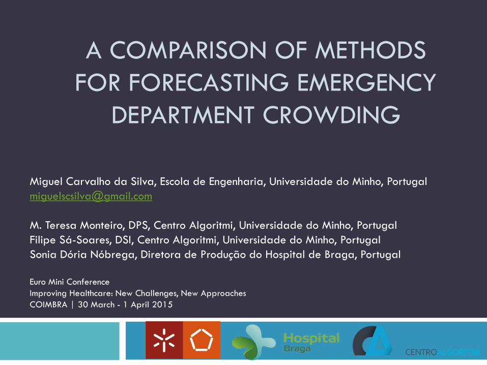
Outline of the talk

Motivation and Objectives

Emergency Department Unit (ED) – Braga’s Hospital

Data

Forecasting Methods

Evaluation Metrics

Computational Tests

Results Analysis

Management Optimization

Limitations & On-going Work

References

Motivation

Patients large influx to ED is an international and

growing problem (Overcrowding), ED arrivals

increase year after year

Great increase in life expectancy, difficulties in

access to primary care, ...

large delays, patient and staff stress, medical errors,

in-hospital infection, abandonment of service, loss of

profit, complaints…

Decrease health service level

Motivation and Objectives

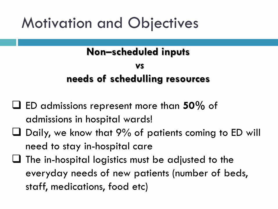
Non–scheduled inputs

vs

needs of schedulling resources

ED admissions represent more than 50% of

admissions in hospital wards!

Daily, we know that 9% of patients coming to ED will

need to stay in-hospital care

The in-hospital logistics must be adjusted to the

everyday needs of new patients (number of beds,

staff, medications, food etc)

Motivation

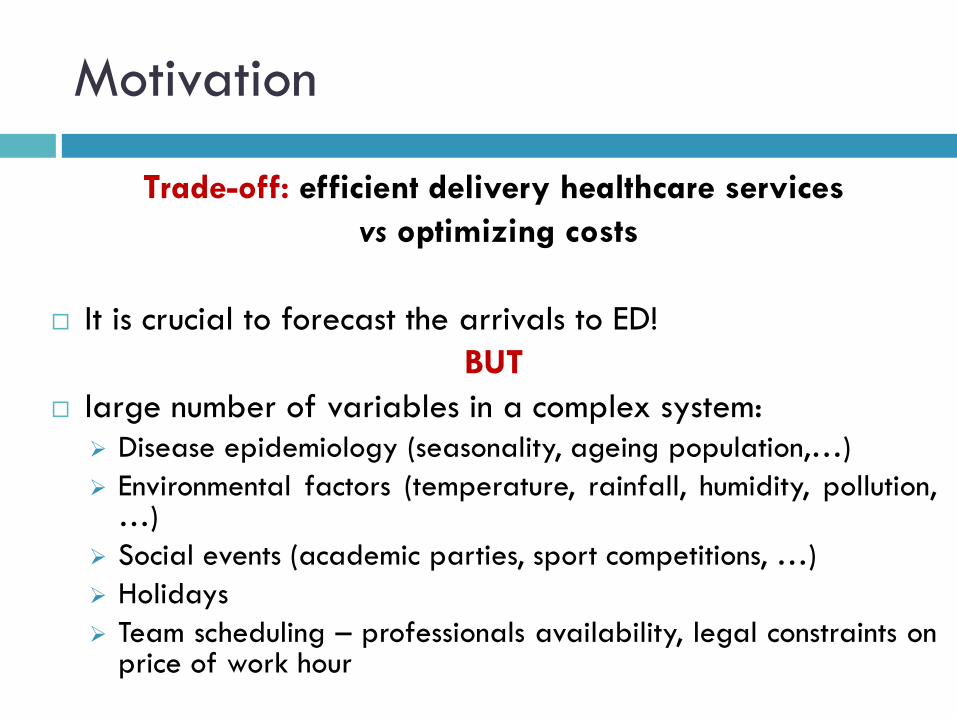
Trade-off: efficient delivery healthcare services

vs optimizing costs

It is crucial to forecast the arrivals to ED!

BUT

large number of variables in a complex system:

Disease epidemiology (seasonality, ageing population,…)

Environmental factors (temperature, rainfall, humidity, pollution, …)

Social events (academic parties, sport competitions, …)

Holidays

Team scheduling – professionals availability, legal constraints on price of work hour

Motivation and Objectives

Metrics based on empirical knowledge can not respond

on time to large variation on arrivals

Forecasting Methods and their comparison:

based on long time series

(use statistical data about recent performance to predict

current and future performance to a short-term)

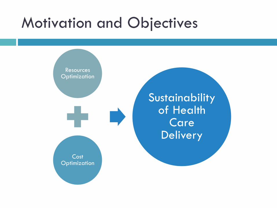
Resources Optimization

Cost Optimization

Sustainability of Health

Care Delivery

Motivation and Objectives

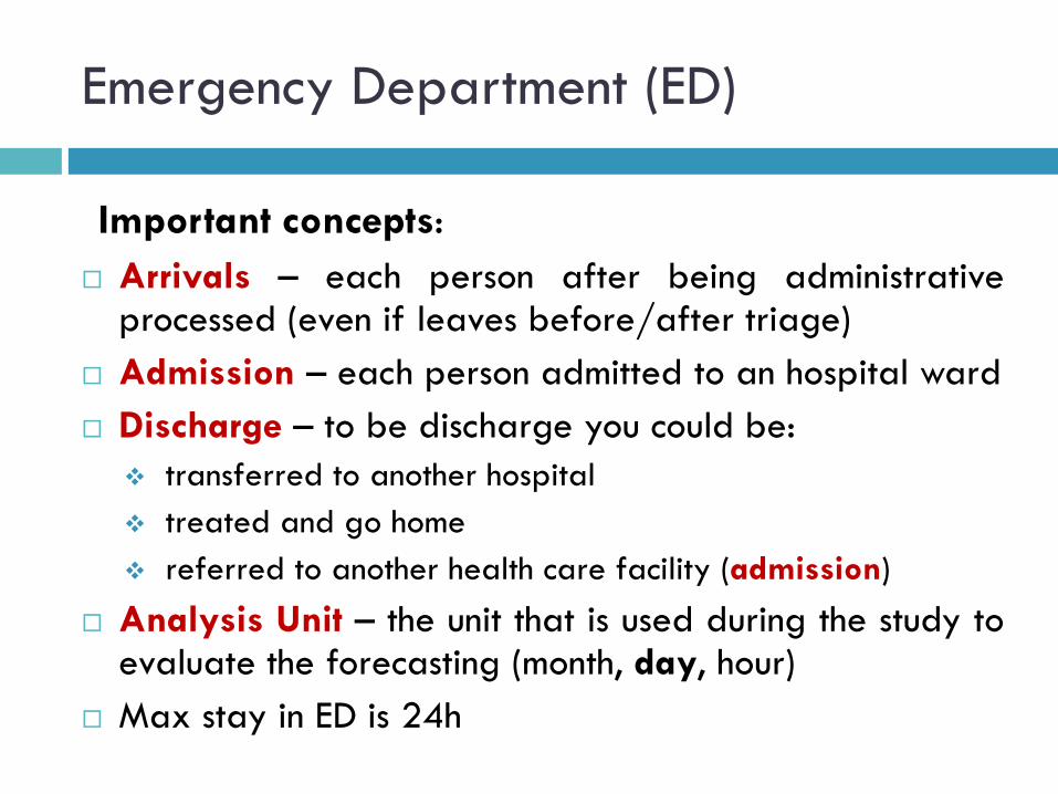
Arrivals – each person after being administrative processed (even if leaves before/after triage)

Admission – each person admitted to an hospital ward

Discharge – to be discharge you could be:

transferred to another hospital

treated and go home

referred to another health care facility (admission)

Analysis Unit – the unit that is used during the study to evaluate the forecasting (month, day, hour)

Max stay in ED is 24h

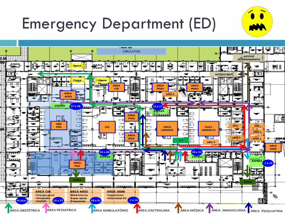
Emergency Department (ED)

Important concepts:

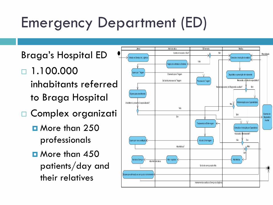
Emergency Department (ED)

Braga’s Hospital ED

1.100.000

inhabitants referred

to Braga Hospital

Complex organization

More than 250

professionals

More than 450

patients/day and

their relatives

Emergency Department (ED)

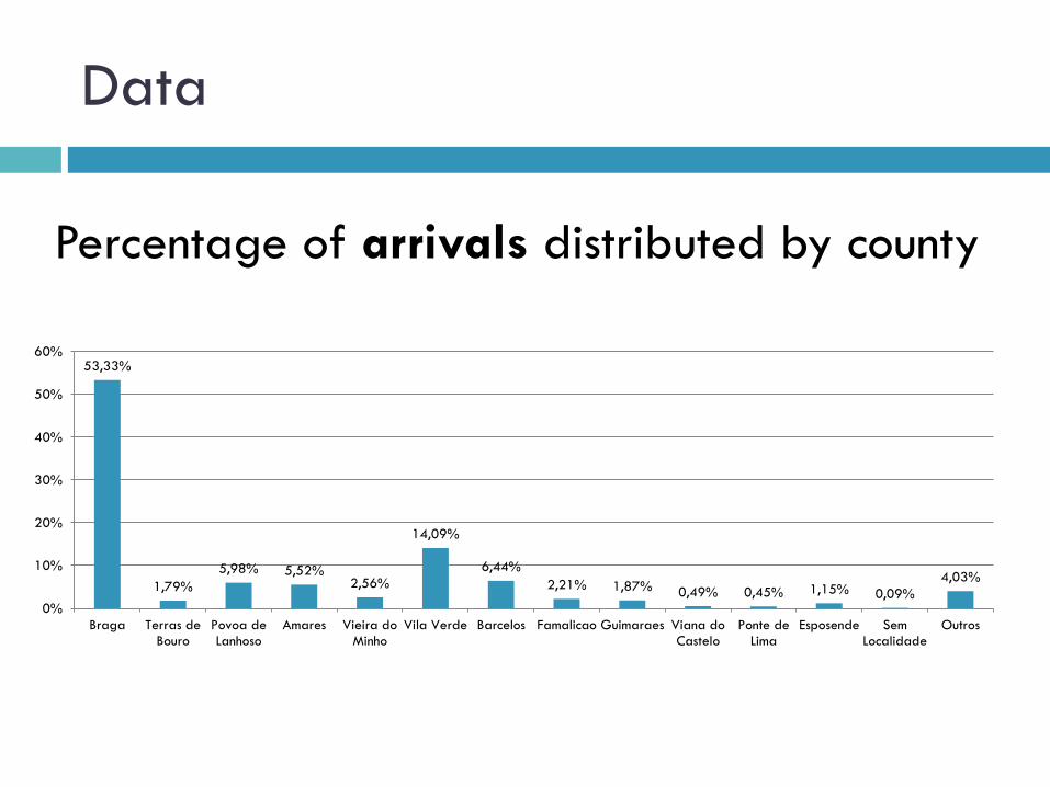
Data

53,33%

1,79%

5,98% 5,52% 2,56%

14,09%

6,44%

2,21% 1,87% 0,49% 0,45% 1,15% 0,09%

4,03%

0%

10%

20%

30%

40%

50%

60%

Braga Terras deBouro

Povoa deLanhoso

Amares Vieira doMinho

Vila Verde Barcelos Famalicao Guimaraes Viana doCastelo

Ponte deLima

Esposende SemLocalidade

Outros

Percentage of arrivals distributed by county

Data

Data collected for users arrivals Jan 2012 - Dec 2014

2012 and 2013 will be used as Test Data

177 769 arrivals in 2012

185 132 arrivals in 2013

Study more than 40 scientific articles: selection the best

methodological choices to the collection and data

analysis

Data collected:

Hour of arrival, triage color, triage destiny, age, sex,

data of arrival, Times between stages inside the ED

department, discharge hour, ...

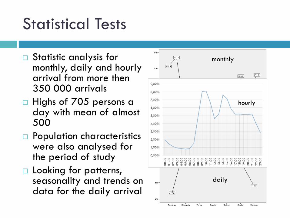
Statistical Tests

Statistic analysis for monthly, daily and hourly arrival from more then 350 000 arrivals

Highs of 705 persons a day with mean of almost 500

Population characteristics were also analysed for the period of study

Looking for patterns, seasonality and trends on data for the daily arrival

daily

monthly

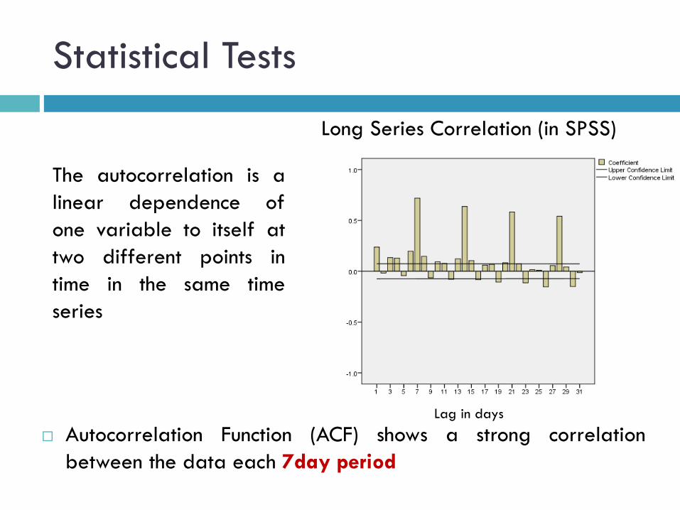
Statistical Tests

Autocorrelation Function (ACF) shows a strong correlation

between the data each 7day period

Long Series Correlation (in SPSS)

Lag in days

The autocorrelation is a

linear dependence of

one variable to itself at

two different points in

time in the same time

series

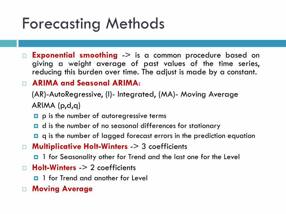
Forecasting Methods

Exponential smoothing -> is a common procedure based on giving a weight average of past values of the time series, reducing this burden over time. The adjust is made by a constant.

ARIMA and Seasonal ARIMA:

(AR)-AutoRegressive, (I)- Integrated, (MA)- Moving Average

ARIMA (p,d,q)

p is the number of autoregressive terms

d is the number of no seasonal differences for stationary

q is the number of lagged forecast errors in the prediction equation

Multiplicative Holt-Winters -> 3 coefficients

1 for Seasonality other for Trend and the last one for the Level

Holt-Winters -> 2 coefficients

1 for Trend and another for Level

Moving Average

Forecasting Methods

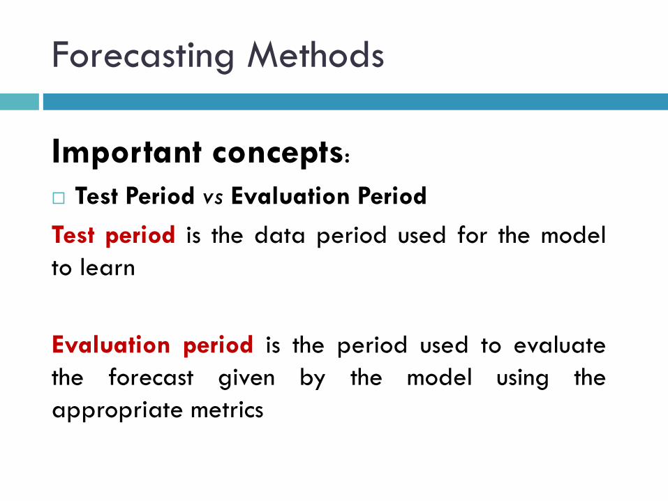
Important concepts:

Test Period vs Evaluation Period

Test period is the data period used for the model

to learn

Evaluation period is the period used to evaluate

the forecast given by the model using the

appropriate metrics

Evaluation Metrics

Evaluation Metrics: to measure and validate the model

forecasting

AIC -> Akaike Information Criteria

BIC -> Bayesian Information Criteria

Based on percentage error:

MAPE -> Mean Absolute Percentage Error

MAD -> Mean Absolute Error

Dependent on the scale

RMSE -> Root Mean Square Error

Evaluation Metrics

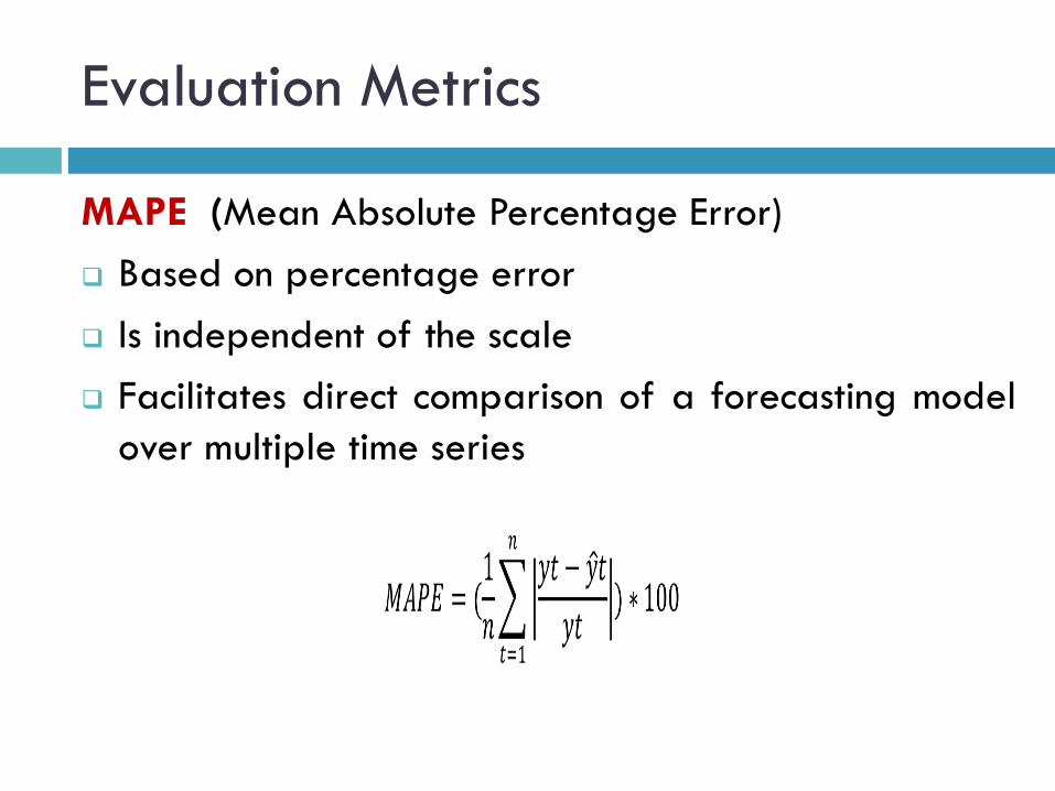
MAPE (Mean Absolute Percentage Error)

Based on percentage error

Is independent of the scale

Facilitates direct comparison of a forecasting model

over multiple time series

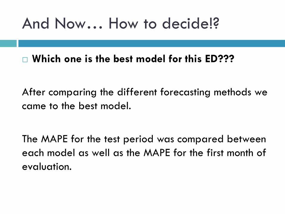
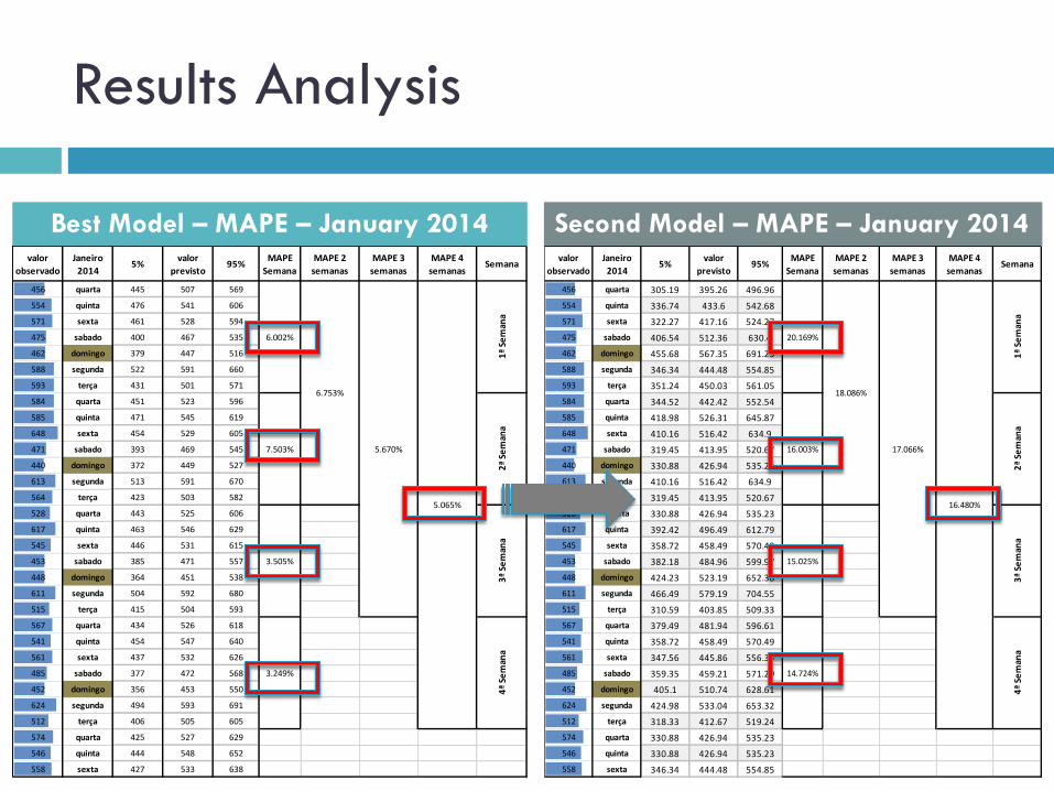
And Now… How to decide!?

Which one is the best model for this ED???

After comparing the different forecasting methods we

came to the best model.

The MAPE for the test period was compared between

each model as well as the MAPE for the first month of

evaluation.

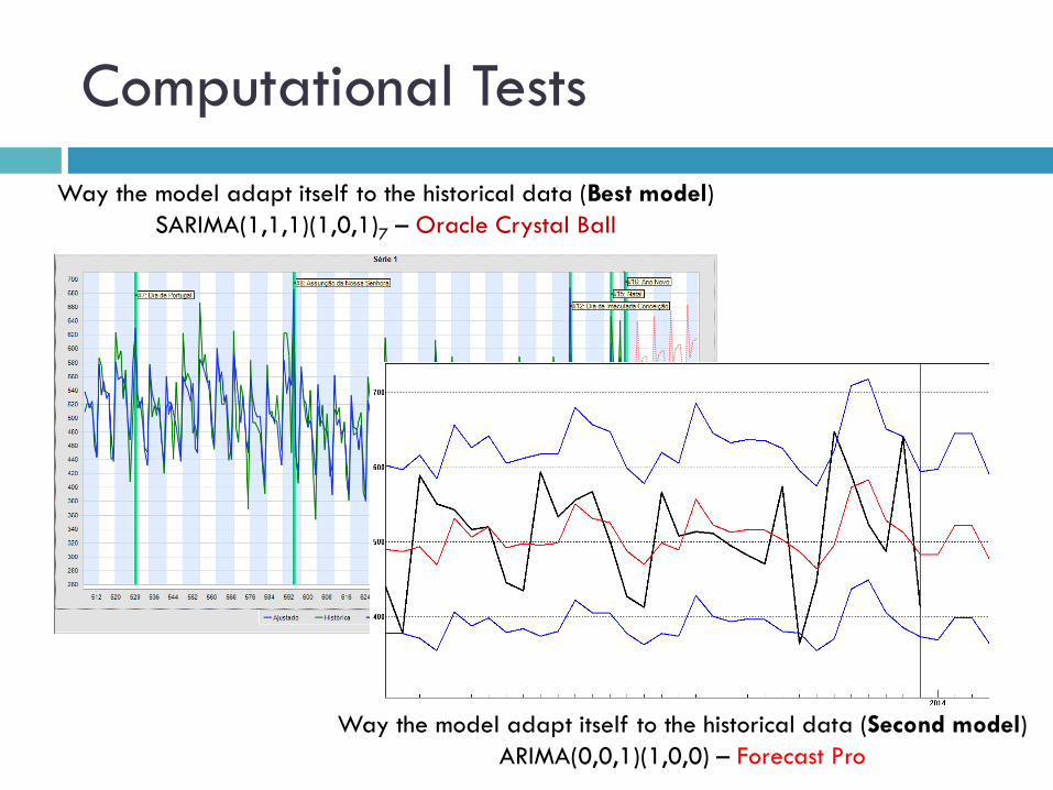
Computational Tests

Way the model adapt itself to the historical data (Best model)

SARIMA(1,1,1)(1,0,1)7 – Oracle Crystal Ball

Way the model adapt itself to the historical data (Second model)

ARIMA(0,0,1)(1,0,0) – Forecast Pro

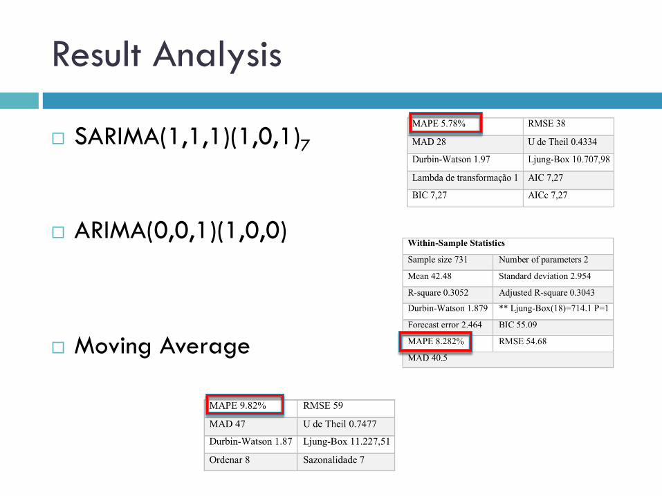
SARIMA(1,1,1)(1,0,1)7

ARIMA(0,0,1)(1,0,0)

Moving Average

Result Analysis

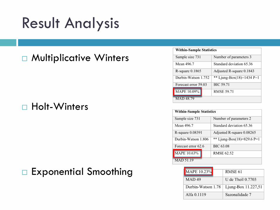
Result Analysis

Multiplicative Winters

Holt-Winters

Exponential Smoothing

Results Analysis

Best Model – MAPE – January 2014 Second Model – MAPE – January 2014 valor

observado

Janeiro

20145%

valor

previsto95%

MAPE

Semana

MAPE 2

semanas

MAPE 3

semanas

MAPE 4

semanasSemana

456 quarta 445 507 569

554 quinta 476 541 606

571 sexta 461 528 594

475 sabado 400 467 535

462 domingo 379 447 516

588 segunda 522 591 660

593 terça 431 501 571

584 quarta 451 523 596

585 quinta 471 545 619

648 sexta 454 529 605

471 sabado 393 469 545

440 domingo 372 449 527

613 segunda 513 591 670

564 terça 423 503 582

528 quarta 443 525 606

617 quinta 463 546 629

545 sexta 446 531 615

453 sabado 385 471 557

448 domingo 364 451 538

611 segunda 504 592 680

515 terça 415 504 593

567 quarta 434 526 618

541 quinta 454 547 640

561 sexta 437 532 626

485 sabado 377 472 568

452 domingo 356 453 550

624 segunda 494 593 691

512 terça 406 505 605

574 quarta 425 527 629

546 quinta 444 548 652

558 sexta 427 533 638

6.002%

7.503%

3.505%

3.249%

6.753%

5.670%

5.065%1

ª Se

man

a2

ª Se

man

a3

ª Se

man

a4

ª Se

man

a

valor

observado

Janeiro

20145%

valor

previsto95%

MAPE

Semana

MAPE 2

semanas

MAPE 3

semanas

MAPE 4

semanasSemana

456 quarta 305.19 395.26 496.96

554 quinta 336.74 433.6 542.68

571 sexta 322.27 417.16 524.27

475 sabado 406.54 512.36 630.4

462 domingo 455.68 567.35 691.25

588 segunda 346.34 444.48 554.85

593 terça 351.24 450.03 561.05

584 quarta 344.52 442.42 552.54

585 quinta 418.98 526.31 645.87

648 sexta 410.16 516.42 634.9

471 sabado 319.45 413.95 520.67

440 domingo 330.88 426.94 535.23

613 segunda 410.16 516.42 634.9

564 terça 319.45 413.95 520.67

528 quarta 330.88 426.94 535.23

617 quinta 392.42 496.49 612.79

545 sexta 358.72 458.49 570.49

453 sabado 382.18 484.96 599.97

448 domingo 424.23 523.19 652.38

611 segunda 466.49 579.19 704.55

515 terça 310.59 403.85 509.33

567 quarta 379.49 481.94 596.61

541 quinta 358.72 458.49 570.49

561 sexta 347.56 445.86 556.39

485 sabado 359.35 459.21 571.29

452 domingo 405.1 510.74 628.61

624 segunda 424.98 533.04 653.32

512 terça 318.33 412.67 519.24

574 quarta 330.88 426.94 535.23

546 quinta 330.88 426.94 535.23

558 sexta 346.34 444.48 554.85

20.169%

16.003%

15.025%

14.724%

18.086%

17.066%

16.480%

1ª

Sem

ana

2ª

Sem

ana

3ª

Sem

ana

4ª

Sem

ana

Results Analysis

501

546 562

350

400

450

500

550

600

650

700

qua

rta

qui

nta

sexta

sab

ado

dom

ing

o

seg

unda

terç

a

qua

rta

qui

nta

sexta

sab

ado

dom

ing

o

seg

unda

terç

a

qua

rta

qui

nta

sexta

sab

ado

dom

ing

o

seg

unda

terç

a

qua

rta

qui

nta

sexta

sab

ado

dom

ing

o

seg

unda

terç

a

qua

rta

qui

nta

sexta

5% Previsto 95% Observado

456

554 571

475 462

588 593 584 585

648

471

440

613

564

528

617

545

453 448

611

515

567

541

561

485

452

624

512

574

546 558

350

400

450

500

550

600

650

700

qua

rta

qui

nta

sexta

sab

ado

dom

ing

o

seg

unda

terç

a

qua

rta

qui

nta

sexta

sab

ado

dom

ing

o

seg

unda

terç

a

qua

rta

qui

nta

sexta

sab

ado

dom

ing

o

seg

unda

terç

a

qua

rta

qui

nta

sexta

sab

ado

dom

ing

o

seg

unda

terç

a

qua

rta

qui

nta

sexta

5% Previsto 95% Observado

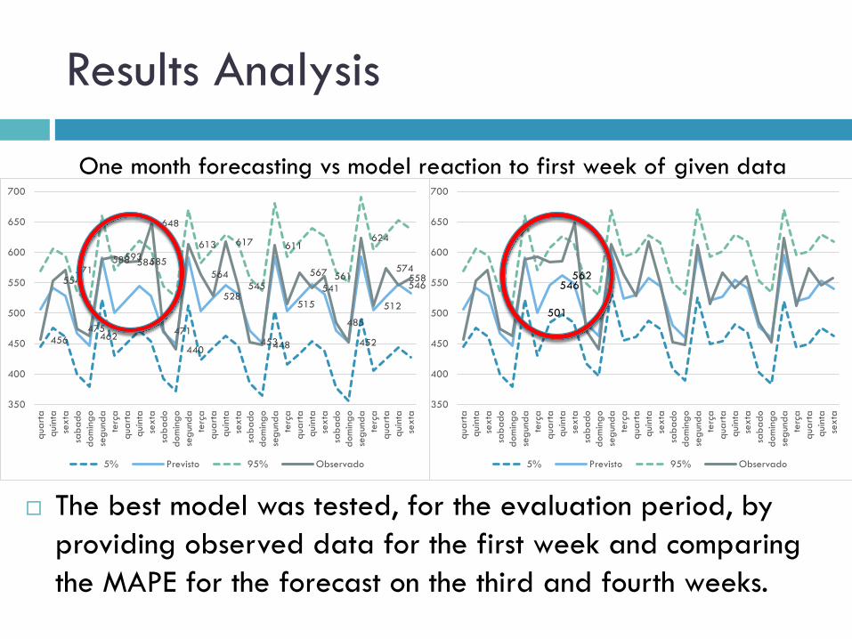
The best model was tested, for the evaluation period, by

providing observed data for the first week and comparing

the MAPE for the forecast on the third and fourth weeks.

One month forecasting vs model reaction to first week of given data

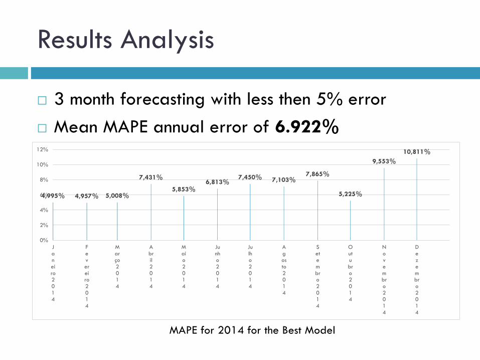
3 month forecasting with less then 5% error

Mean MAPE annual error of 6.922%

4,995% 4,957% 5,008%

7,431%

5,853% 6,813%

7,450% 7,103% 7,865%

5,225%

9,553%

10,811%

0%

2%

4%

6%

8%

10%

12%

Janeiro2014

Fevereiro2014

Março2014

Abril2014

Maio2014

Junho2014

Julho2014

Agosto2014

Setembro2014

Outubro2014

Novembro2014

Dezembro2014

Results Analysis

MAPE for 2014 for the Best Model

350

400

450

500

550

600

650

700

750

qua

rta

terç

ase

gun

da

dom

ing

o

sab

ado

sexta

qui

nta

qua

rta

terç

a

seg

unda

dom

ing

o

sab

ado

sexta

qui

nta

qua

rta

terç

a

seg

unda

dom

ing

o

sab

ado

sexta

qui

nta

qua

rta

terç

a

seg

unda

dom

ing

o

sab

ado

sexta

qui

nta

qua

rta

terç

a

seg

unda

dom

ing

o

sab

ado

sexta

qui

nta

qua

rta

terç

a

seg

unda

dom

ing

o

sab

ado

sexta

qui

nta

qua

rta

terç

a

seg

unda

dom

ing

o

sab

ado

sexta

qui

nta

qua

rta

terç

a

seg

unda

dom

ing

o

sab

ado

sexta

qui

nta

qua

rta

terç

a

seg

unda

dom

ing

o

sab

ado

Observado Previsto

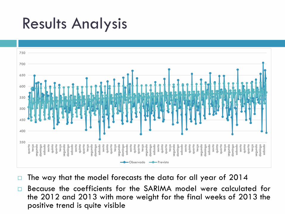
Results Analysis

The way that the model forecasts the data for all year of 2014

Because the coefficients for the SARIMA model were calculated for the 2012 and 2013 with more weight for the final weeks of 2013 the positive trend is quite visible

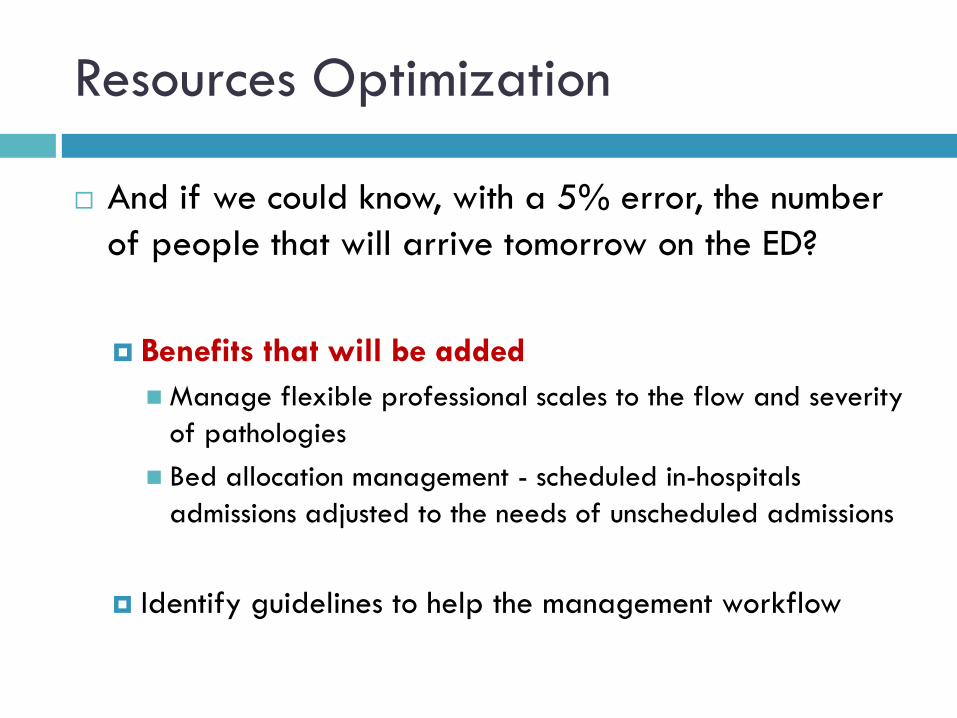
Resources Optimization

And if we could know, with a 5% error, the number

of people that will arrive tomorrow on the ED?

Benefits that will be added

Manage flexible professional scales to the flow and severity

of pathologies

Bed allocation management - scheduled in-hospitals

admissions adjusted to the needs of unscheduled admissions

Identify guidelines to help the management workflow

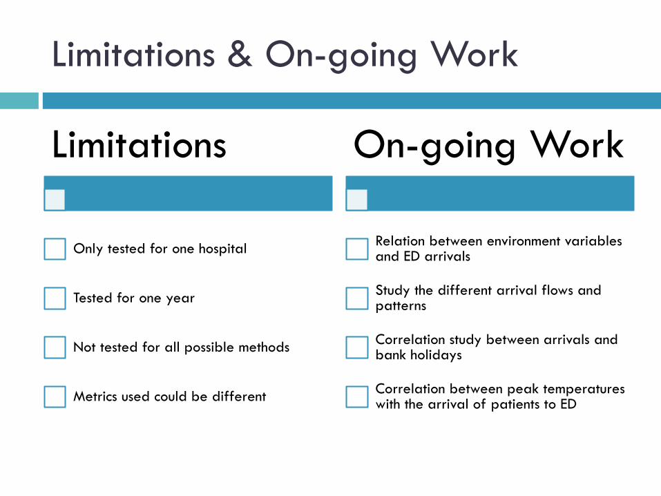
Limitations & On-going Work

Limitations

Only tested for one hospital

Tested for one year

Not tested for all possible methods

Metrics used could be different

On-going Work

Relation between environment variables and ED arrivals

Study the different arrival flows and patterns

Correlation study between arrivals and bank holidays

Correlation between peak temperatures with the arrival of patients to ED

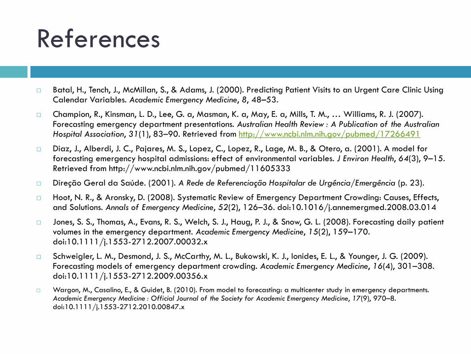
References

Batal, H., Tench, J., McMillan, S., & Adams, J. (2000). Predicting Patient Visits to an Urgent Care Clinic Using Calendar Variables. Academic Emergency Medicine, 8, 48–53.

Champion, R., Kinsman, L. D., Lee, G. a, Masman, K. a, May, E. a, Mills, T. M., … Williams, R. J. (2007). Forecasting emergency department presentations. Australian Health Review : A Publication of the Australian Hospital Association, 31(1), 83–90. Retrieved from http://www.ncbi.nlm.nih.gov/pubmed/17266491

Diaz, J., Alberdi, J. C., Pajares, M. S., Lopez, C., Lopez, R., Lage, M. B., & Otero, a. (2001). A model for forecasting emergency hospital admissions: effect of environmental variables. J Environ Health, 64(3), 9–15. Retrieved from http://www.ncbi.nlm.nih.gov/pubmed/11605333

Direção Geral da Saúde. (2001). A Rede de Referenciação Hospitalar de Urgência/Emergência (p. 23).

Hoot, N. R., & Aronsky, D. (2008). Systematic Review of Emergency Department Crowding: Causes, Effects, and Solutions. Annals of Emergency Medicine, 52(2), 126–36. doi:10.1016/j.annemergmed.2008.03.014

Jones, S. S., Thomas, A., Evans, R. S., Welch, S. J., Haug, P. J., & Snow, G. L. (2008). Forecasting daily patient volumes in the emergency department. Academic Emergency Medicine, 15(2), 159–170. doi:10.1111/j.1553-2712.2007.00032.x

Schweigler, L. M., Desmond, J. S., McCarthy, M. L., Bukowski, K. J., Ionides, E. L., & Younger, J. G. (2009). Forecasting models of emergency department crowding. Academic Emergency Medicine, 16(4), 301–308. doi:10.1111/j.1553-2712.2009.00356.x

Wargon, M., Casalino, E., & Guidet, B. (2010). From model to forecasting: a multicenter study in emergency departments. Academic Emergency Medicine : Official Journal of the Society for Academic Emergency Medicine, 17(9), 970–8. doi:10.1111/j.1553-2712.2010.00847.x

A COMPARISON OF METHODS

FOR FORECASTING EMERGENCY

DEPARTMENT CROWDING

Miguel Carvalho da Silva, Escola de Engenharia, Universidade do Minho, Portugal

miguelscsilva@gmail.com

M. Teresa Monteiro, DPS, Centro Algoritmi, Universidade do Minho, Portugal

Filipe Sá-Soares, DSI, Centro Algoritmi, Universidade do Minho, Portugal

Sonia Dória Nóbrega, Diretora de Produção do Hospital de Braga, Portugal

Euro Mini Conference

Improving Healthcare: New Challenges, New Approaches

COIMBRA | 30 March - 1 April 2015