COMPARISON OF FINITE ELEMENT ANALYSES OF A

PIPING TEE USING NASTRAN AND CORTES/SA

Antonio J. Quezon.and Gordon C. EverstineDavid W. Taylor Naval Ship Research and Development Center

SUMMARY

A comparison of finite element analyses of a 24" x 24" x 10" piping teewas made using NASTRAN and CORTES/SA, a modified version of SAP3 having aspecial purpose input processor for generating geometries for a wide variety oftee joints. Four finite element models were subjected to force, moment, andpressure loadings. Flexibility factors and principal stresses were computedfor each model and compared with results obtained experimentally by CombustionEngineering, Inc. Of the four models generated, the first was generated fromactual measured geometry using GPRIME, a geometric and finite element modelingsystem developed at DTNSRDC. The other three models were generated from anidealized tee using the data generator contained in CORTES/SA.

The generation of an idealized tee proved to be very easy and inexpensivecompared to generation from actual geometry, and, when analyzed by NASTRAN,proved adequate. Results from the NASTRAN analyses were in good agreementwith experimental results for all loadings except internal pressure. TheCORTES/SA analyses gave good results for the internal pressure loading, butpoorer results for out-of-plane bending moments or forces resulting in out-of-plane bending. Two of the basic load cases in CORTES/SA were found to containerrors that could.not be easily corrected. A cost comparison of NASTRAN andCORTES/SA showed NASTRAN to be less expensive to run than CORTES/SA foridentical meshes. Overall, considering modeling effort, cost, and accuracy, itis concluded that tees can be easily and accurately analyzed by NASTRAN usingan idealized mesh generated by CORTES/SA.

BACKGROUND

The designer of a piping system requires a knowledge of the deflectionsand stresses caused throughout the system by anticipated service loads. Ofparticular interest are critical components such as elbows and tees.

The purpose of this paper is to summarize the results of a study (ref. 1)made recently to assess the effectiveness of the finite element method (FEM) inpredicting flexibility factors and stresses in piping tees subjected to force,moment, and pressure loadings. A similar study (ref. 2), performed for pipingelbows, indicated that very good agreement could be expected between FEM

224

https://ntrs.nasa.gov/search.jsp?R=19800025287 2018-04-06T03:39:41+00:00Z

analysis and experiment. Tees, although conceptually no more difficult toanalyze than elbows, are considerably more complicated geometrically. Areducing tee, for example, has in the crotch region a fillet with a variableradius of curvature as well as variable thickness. Moreover, the adjacentstraight sections may not be cylindrical. Thus, geometrical idealizations oftees, although plausible, may be incorrect.

The finite element analyses described here involve idealized models as wellas a model based on actual measured geometry. Two computer programs were usedfor the analyses: NASTRAN, a widely-used general purpose finite elementstructural analysis program, and CORTES/SA (ref. 3), a special purpose finiteelement tee analysis program based on SAPS and written at the University ofCalifornia at Berkeley under the sponsorship of the Oak Ridge NationalLaboratory.* This series of analyses was designed to provide information onthe sensitivity of the results to various mesh densities as well as on theadequacy of the assumed idealizations.

In this paper, the program CORTES/SA will be referred to by theabbreviated name "CORTES".

STATEMENT OF THE PROBLEM

Combustion Engineering, Inc., performed an experimental stress analysis(ref. 4) on an ANSI B16.9 carbon steel tee designated T-12. Pipe extensionswere welded to the branch and run ends of the tee, and the resulting assemblywas placed in a load frame. One of the run ends was built in to represent afixed end, and the other run end and the branch end were used to apply sixorthogonal moments and five orthogonal forces. Internal pressure was alsoapplied. Table 1 and Figure 1 summarize the applied loads. Load case 4 (F3X)was not tested because of strength limitations of the load frame. Stress datafor all twelve load cases were gathered from strain gages fixed on specificrows on the tee (Figure 2) and were plotted against normalized surface distance.

The tee analyzed was a reducing tee with a 24-inch-diameter run end and a10.75-inch-diameter branch. Loads to the run were applied at the free end ofthe run pipe extension, 173 inches from the branch-run intersection (Figure 1).Loads to the branch were applied at the end of the branch pipe extension,77 inches from the branch-run intersection. The run pipe extension consistedof 24-inch-diameter schedule 40 (0.687-inch nominal wall thickness) carbonsteel piping. The branch pipe extension consisted of 10.75-inch-diameterschedule 40 (0.365-inch nominal wall thickness) carbon steel piping.

The finite element analyses of the tee simulated these loading conditionsso that stresses at selected locations could be compared to the experimental

*The CORTES package of computer programs is distributed as program number 759

by the National Energy Software Center (NESC), Argonne National Laboratory,9700 S. Cass Avenue, Argonne, Illinois 60439.

225

results. For most load cases, the strain gage rows (Figure 2) selected forcomparison were those on which the peak stresses occurred.

ANALYSES PERFORMED

NASTRAN analyses were performed for the first three models generated, andCORTES analyses were performed for the third and fourth models. These fivefinite element analyses are summarized in Table 2. In the abbreviations Nl,N2, N3, C3, and C4 used to identify the analyses, the first character (N or C)indicates the analysis program used (NASTRAN or CORTES), and the secondcharacter indicates the mesh used. A typical mesh generated by CORTES isshown in Figure 3. In general, a higher mesh number corresponds to a finermesh, either overall or in selected key regions of the tee.

. The NASTRAN analysis of Mesh 1 was the only analysis performed for a modelgenerated from actual measured geometry. The remaining analyses were performedeither by NASTRAN or by CORTES on meshes generated by CORTES assuming anidealized geometry. In all cases only one-fourth of the actual tee was modeleddue to symmetry.

For the NASTRAN analyses, the tee, including pipe extensions, was modeledwith plate (NASTRAN QUAD2) elements. Flexible beam (BAR) elements werearranged in a spoke formation radiating from an imaginary point in the centerof the cross section at the ends of the tee branch and run to facilitate thecalculation of the average rotation of these cross sections. Rigid (RIGD1)elements were defined at the ends of the pipe extensions for use in loadapplication. The loads were applied to a point in the center of the rigidcross section at the ends of the pipe extensions.

In the CORTES analyses, the tee and pipe extensions were modeled using an8-node hexahedral element. This element, designated ZIB8R9, is a modificationof the standard Zienkiewicz-Irons isoparametric element and, according toGantayat and Powell (ref. 3), has bending properties superior to those of theunmodified isoparametric element.

Mesh 1 was modeled from actual geometry as specified in the CombustionEngineering, Inc., report (ref. 4) which tabulated coordinates of points on theouter surface of the tee and thicknesses at these points. From thesedigitized data, a general B-spline surface was fitted through the suppliedpoints using the geometric and finite element modeling processor GPRIME(refs. 5 and 6). Once this geometric model was defined, GPRIME was used togenerate a finite element mesh which included the effects of variablethicknesses.

Meshes 2 through 4 were modeled as idealized tee joints using the auto-matic mesh generation routine in CORTES. The tee joint is idealized byshallow cones representing the branch and run portions of the tee, connectedto each other through an analytically defined transition fillet (ref. 3).

226

STRESS RESULTS

The results of primary interest are normalized principal stress valuesfor elements in particular locations on the tee. The peak normalizedprincipal stress was plotted against surface distance ratio for each load caseand compared to the experimental results obtained by Combustion Engineering,Inc. (ref. 4).

The tee analyzed by Combustion Engineering, Inc., was heavily instru-mented, both internally and externally, with strain gages in two of the fourquadrants. The gages in each quadrant were arranged in six rows as shown inFigure 2. Since the peak stresses for most load cases occurred on row 1 orrow 6, analytical and experimental results were compared for these rows only.

For each load case, the analytical results for principal stresses werenormalized by a stress calculated from beam theory, as indicated in Table 1.The normalized principal stresses were then plotted against the surface distanceratios of the elements lying on row 1 and row 6.

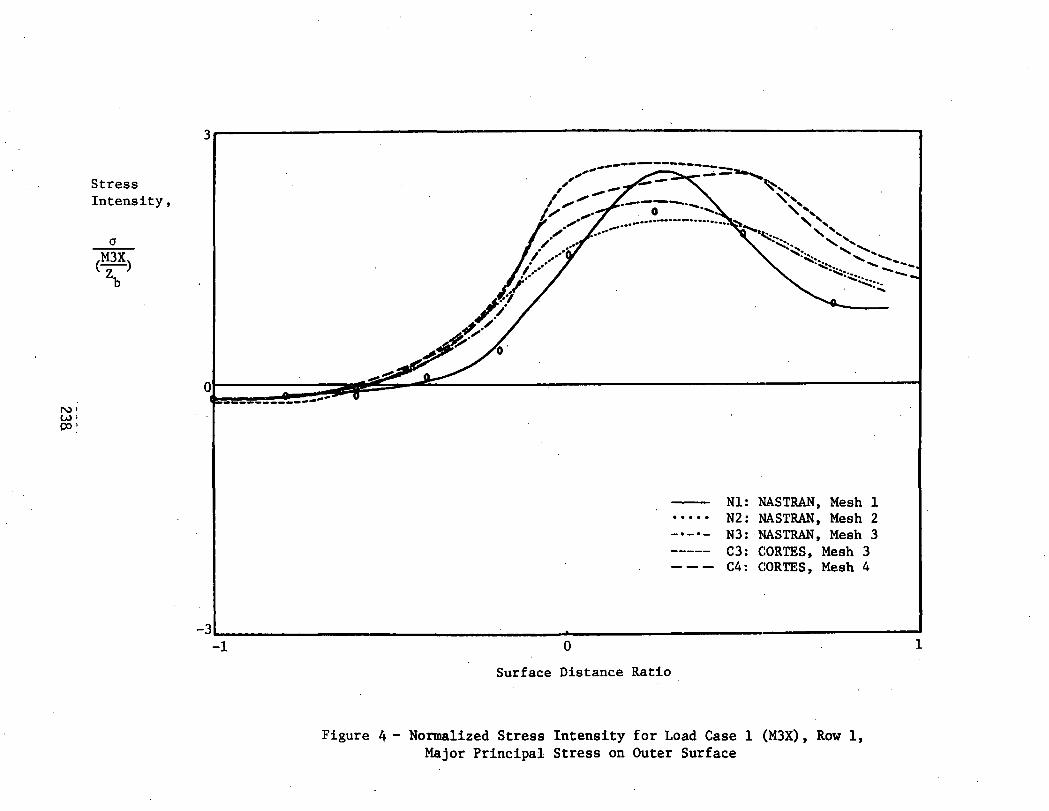
Stress plots for several typical load cases are shown in Figures 4through 8. (Ref. 1 contains plots for all load cases.) All finite elementcurves are smoothed slightly by fitting B-spline curves (refs. 7 and 8) throughthe computed values, which are located at element centroids for the NASTRANresults and at grid points for the CORTES results.

FLEXIBILITY FACTORS

Two ambiguities were encountered in comparing computed flexibility factorswith experimental results obtained by Combustion Engineering, Inc. Theseambiguities involved the definition of flexibility factors and the way in whichthe rotation of branch or run end cross sections was measured. CombustionEngineering, Inc., defined the flexibility factors as

e - e_ meas corr

0nom

where

6 = measured rotation at an intermediate location on the pipeTtlpog • .

extension

6 = rotation correction computed by simple beam theory for the lengthC0rr of pipe between the tee weld line and the location at which the

rotation is actually measured

6 = nominal rotation computed by simple beam theory for the distancebetween the tee weld lines where

227

9 = — (for bending moments) (2)nom c> i

TL6 = — (for torsional moments) (3)nom JG

PL26nom = 2EI (f°r P°int loads) (4)

Since Combustion Engineering, Inc., could not measure the actual rotationsat the branch and run end cross sections, measurements were made at otherlocations on the pipe extensions and then corrected to the branch and run endsusing simple beam theory. On the other hand, the NASTRAN analyses used veryflexible beam elements radiating from an imaginary point in the center of thebranch and run end cross sections to the points on the circumference of thebranch and run ends. This modeling technique allowed an approximate averagerotation for the cross sections to be easily obtained for the imaginary centerpoint. However, because plane sections do not, under loading, remain plane,there is no single rotation for a section, so that different methods forcomputing rotations will yield different results.

For the computation of flexibility factors from the NASTRAN results, therelation

6 ,

k-e^- ' ' (5)nom

was used, where

6 = computed relative rotation of end "a" with respect to end "b"3-D

0 = nominal rotation computed by beam theory for the rotation of endnom "a" with respect to end "b"

Flexibility factors were computed for the free branch and run ends withrespect to the fixed run end for each load case except for F2X (an axial loadon the run) and internal pressure, neither of which causes any significantrotation. For example, the flexibility factor for a rotation about the X-axisof the branch end with respect to the fixed run end is denoted by kx31> wnere

the X in the subscript represents the axis of rotation, the 3 represents thebranch end, and the 1 represents the fixed run end. For each load case,flexibility factors for each cross section were computed.

Table 3 compares the flexibility factors computed from the three NASTRANanalyses to the experimental values. The computed flexibility factors comparereasonably well for most load cases, an exception being -z2I ^or ^oa^ case 5(F3Y) of N2. Combustion Engineering, Inc., did not compute flexibility factorsfor this load case because the stresses and deflections were considered toosmall to give reliable answers. The displacements computed in the threeNASTRAN analyses for load case 5, however, did not appear to be significantlysmaller than those of the other load cases, although the run end of the tee did

228

warp severely in all three analyses. Since the distortions in all threeanalyses were similar, it appears to have been due to chance that the flexibil-ity factors for Nl and N3 were not also negative for this load case. Thisimplies that any method used to compute a single rotation of the run end isinadequate for severely distorted cross sections. Moreover, the usefulness ofa flexibility factor when severe cross-sectional distortion occurs isquestionable.

In general, a negative flexibility factor, whether arising from experimentor analysis, is physically impossible, since such a factor implies a rotationin a direction opposite to that of the applied moment. Negative values canarise experimentally whenever rotations measured at one location have to be"corrected" (using beam theory) to yield rotations elsewhere. Negative valuescan result from a finite element analysis whenever severe cross-sectionaldistortion occurs, in which case the usefulness of an "average" rotation of thecross section is in doubt.

DISCUSSION OF RESULTS AND CONCLUSIONS

The three NASTRAN analyses of the tee joint were generally in very goodagreement with the experimental results and accurately predicted peak stressesfor most loadings except load cases 3 (M3Z) and 13 (pressure). Also, asexpected, the agreement with the experimental results improved with finermeshes. In general, the two CORTES analyses were slightly less accurate thanthe NASTRAN analyses except for load case 13 (pressure). We are unable toexplain this behavior. While the CORTES results for pressure loading weresignificantly better than NASTRANfs, the results for load cases 1 (M3X),8 (M2Y), 10 (F2X), and 12 (F2Z) were worse. Note that most of these load casesinvolve either out-of-plane bending moments or forces resulting in out-of-planebending. The CORTES analyses of load cases 6 (F3Z) and 7 (M2X) were also foundto contain errors in formulation and coding which could not be easilycorrected.

The preparation of the NASTRAN model of mesh 1 (called Nl) was the mosttime-consuming and expensive of all the models, since this mesh was generatedfrom actual geometry. Although the Nl calculations for all load cases exceptpressure (Figure 8) are in very good agreement with the experimental results,they are not significantly better than those obtained from the other analyses,so the extra effort is not justified.

In a comparison of NASTRAN and CORTES analyses of an identical mesh(Mesh 3), the NASTRAN results (N3) were more consistent and predicted peakstresses more accurately than CORTES for ten of the twelve load cases. Onlyfor M3Z and pressure (Fig. 8) did C3 do better than N3. Although N3 was lessexpensive than C3 in computer costs, it required slightly more time for inputpreparation.

Since N3 was in generally better agreement with experimental results thanC3, a coarser mesh (Mesh 2) was also analyzed by NASTRAN (N2) and compared

229

with C3. In all but three of the load cases, M3Z, F3Y, and pressure, N2 wasagain in better agreement with experimental results than C3. Computer costsfrom N2 were significantly less than those for C3, as indicated in Table 2.

In an effort to obtain better results from CORTES, a much finer mesh(Mesh 4) was generated and analyzed, so that the results could be compared withN3. This time, overall performance was about equal for the two analyses,although C4 achieved better results than N3 for M3Z, F3Y, M2Z, F2Y, andpressure.

In conclusion, it is apparent that GPRIME. although well-suited in generalto the generation of tee meshes based on actual geometry, is more difficultand time-consuming to use than the special purpose idealized tee generatorcontained in CORTES. Models based on actual geometry also require geometricdata that would probably not be generally available to the analyst. For thesereasons, CORTES generation of a finite element model based on idealizedgeometry appears to be acceptable. However, if an analyst is interested in anF3Z or an M2X loading, CORTES should not be used as the analyzer because theprogram currently contains errors in the coding of these two load cases. Also,as shown by the comparison of N3 with C4, CORTES requires a mesh about 20%finer to obtain results as accurate as NASTRAN.

Overall, considering modeling effort, cost, and accuracy, it is concludedthat tees can be easily and accurately analyzed by NASTRAN using an idealizedmesh generated by CORTES/SA.

230

REFERENCES

1. Quezon, A.J.; Everstine, G.C.; and Golden, M.E^: Finite Element Analysisof Piping Tees. Report DTNSRDC/CMLD-80/11, David W. Taylor Naval ShipResearch and Development Center, Bethesda, Maryland, June 1980.

2. Marcus, M.S.; and Everstine, G.C.: Finite Element Analysis of Pipe Elbows.Report DTNSRDC/CMLD-79/15, David W. Taylor Naval Ship Research andDevelopment Center, Bethesda, Maryland, Feb. 1980.

3. Gantayat, A.N.; and Powell, G.H.: Stress Analysis of Tee Joints by theFinite Element Method. Report No. US SESM 73-6, Structural EngineeringLaboratory, Univ. of California, Berkeley, California, Feb. 1973.

4. Henley, D.R.: Test Report on Experimental Stress Analysis of a 24"Diameter Tee (ORNL T-12). Report CENC 1237, ORNL-Sub-3310-4, CombustionEngineering, Inc., Chattanooga, Tennessee, Apr. 1975.

5. Golden, M.E.: Geometric Structural Modelling: A Promising Basis for FiniteElement Analysis. Trends in Computerized Structural Analysis andSynthesis, ed. by A.K. Noor and H.B. McComb, Jr., Pergamon Press,Oxford, England, May 1978, pp. 347-350.

6. Golden, M.E.: The Role of a Geometry Processor in Structural Analysis.New Techniques in Structural Analysis by Computer, ed. by R. Melosh andM. Salama, Preprint 3601, ASCE Convention and Exposition (2-6 Apr 1979),American Society of Civil Engineers, Boston, MA, pp. F1-F17.

7. McKee, J.M.; and Kazden, R.J.: G-Prime B-Spline Manipulation Package—Basic Mathematical Subroutines. DTNSRDC Report 77-0036, David W. TaylorNaval Ship Research and Development Center, Bethesda, Maryland, Apr. 1977.

8. McKee, J.M. : Updates to the G—Prime B-Spline Manipulation Package—26 October 1977. Periodic updates available from the author at theDavid W. Taylor Naval Ship Research and Development Center, Bethesda,Maryland 20084.

231

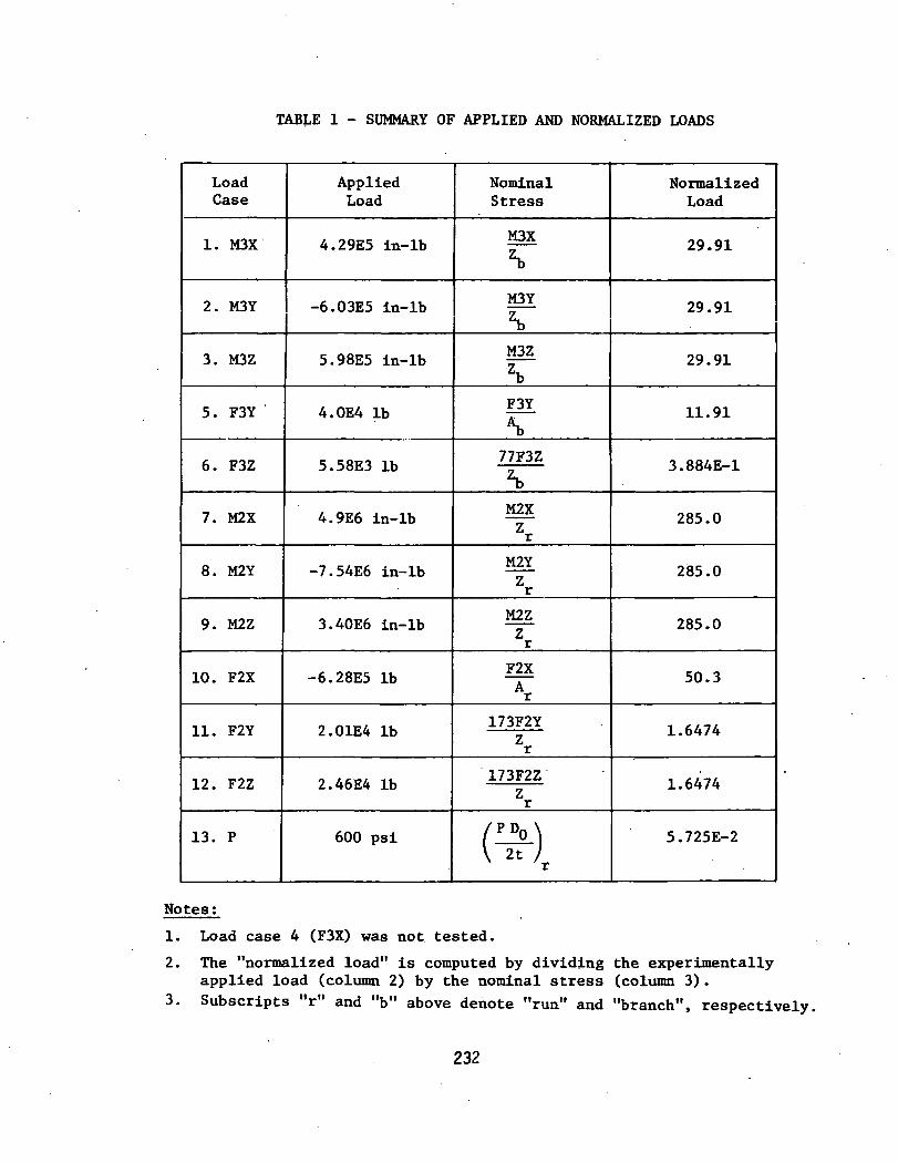
TABLE 1 - SUMMARY OF APPLIED AND NORMALIZED LOADS

LoadCase

1. M3X

2 MO.V

3 wO"7. MoZ,

5 T7O.V• r jl

6 1707. C Jfi

7 KTOV. riZA

8 VTOV• pizi

9 MO 7. MZZ,

1U. rZX

1 1 T?9V11. r/l

1 9 T?071Z . r Lit

13. P

AppliedLoad

4.29E5 in-lb

A fl O.T7 A « 11*.— O.UJHJ in— J.D

5 QQT7C J _ 1 -L. yoKj in— ID

4 ni? /• 11*. Uli't ID

5 CQTJO TV. jtthjj ID

4 Q17^ 4*« 11*. yiib in— lb

i c;/. c-t .«.« iv— / . j'fr.o in— ib

3 /IH17& 4 « 11*.M-Uto in— lb

6 OQTC 1 -r.ZoEj lb

2 m -17 / -i -t. Ulr<4 ib

2 /1 ATT/i 1 V.to Jit ID

600 psi

NominalStress

M3X

Zb

M3YZb

M3ZZb

F3Y

*b

77F3Z

\

M2XZr

M2YZ

M2ZZ

F2XA

173F2YZ

173F2ZZ

F2-),

NormalizedLoad

29.91

OQ Q1zy . yi

OQ Q1/? . yi

n QI. yi

3 0 Q/. i? i.oo'f is— 1

o QC nZOD. U

o be nZo.) .U

OQC rtZoj .U

^n tjU.j

I A/i 7/i.OI/H

1 AA7A.Ot / 1

5.725E-2

Notes;

1. Load case 4 (F3X) was not tested.

2. The "normalized load" is computed by dividing the experimentallyapplied load (column 2) by the nominal stress (column 3).

3. Subscripts "r" and "b" above denote "run" and "branch", respectively.

232

TABLE 2 - COMPARISON OF FINITE ELEMENT ANALYSES:NASTRAN vs. CORTES

NASTRAN orCORTESAnalysis

Idealized orActualGeometry

Number ofElements

Number ofNodes

Number ofDegrees ofFreedom

Total CPSeconds(CDC 6400)

Cost

Nl

NASTRAN

Actual

432

484

2525

2213

$228

N2

NASTRAN

Idealized

420

473

2462

2200

$226

N3

NASTRAN

Idealized

525

583

3047

3135

$335

C3

CORTES

Idealized

549

609

3458

3310

$421

C4

CORTES

Idealized

626

689

3958

4748

$605

233

TABLE 3 - COMPARISON OF FLEXIBILITY FACTORS OFEXPERIMENTAL RESULTS TO NASTRAN RESULTS

LoadCase

1. M3X

2. M3Y

3. M3Z

5. F3Y

6. F3Z

7. M2X

8. M2Y

9. M2Z

11. F2Y

1 0 TPO1?1Z. VLL

kSubscript

X21

X31

Y21

Y31

Z21

Z31

Z21

Z31

X21

X31

X21

X31

Y21

Y31

Z21

Z31

Z21

Z31

Y21

Y31

Experiment

-0.8

1.8

0.5

-0.3

0.5

0.9

1.8

-0.4

-0.5

0.7

0.6

0.9

0.8

0.8

0.8

0.7

0.7

Nl

0.82

2.40

0.72

0.32

0.73

0.90

1.22

1.97

0.85

2.97

0.82

0.82

0.72

0.72

0.73

0.73

0.73

0.83

0.72

0.91

N2

1.00

4.00

0.76

0.33

1.03

0.85

-1.35

0.51

1.09

4.94

1.00

1.00

0.76

0.76

1.01

1.01

1.01

1.08

0.76

0.89

N3

0.85

2.73

0.77

0.32

0,93

0.84

1,53

2.08

0,88

3.40

0.85

0.85

0.77

0.77

0.93

0.93

0.93

1.01

0.77

0.94

234

-J<W

•svO0)0)U1-1O

(aH0)0)H(0

•3TJ0)a.

14-1Oa)•§en

235

Y-AXIS

1I/ Crotchline

— — ^ ^' si' ~~ if \ t ^*^ _ \

-— ^' -•— -i'"^^/ ^^-XL 1

^^, """^^ X.

V^ Xx"\ x.\\ \\l^ \

\ x,\\,\-\

1IS l RUN

1

' R O W 6r^ • >t I

r'' /— i

-1 )

'ROW s

-i'** ROW 4

it-ROW AOWZ ROW 3

X-AXiS

Source: Figure 4, Ref. 4

Figure 2 - Location of Strain Gage Rows on Test Tee

236

CM00

o0)oa)N60c•HCO0)0)H<UT

3

•HCICO0)VI

00

237

o•H4J0)oe0)4-10)•HQQ)Uctf>4-lMCO

X!

en2O)

0)03

O<uM

4J

o a

M-l

O

>> c•u o•HS

O]

CO0)

0)4-1

VIC

*J

H C

O

0) C

O01

O.

M

-H4J

OC

O

C•H•O

H

<U PLI

N•H

JJ

a

(0 0}

co C

(U

(UV

I 4J

4J

C

CM

C

O

\.co coW

W...... H

H

co co co erf prf<! <

! O

O55

Z %

U O

iH

CM

CO

en

<f2! J

S Z

O

U

o>uCO0)oCOM

-lt-l3en

CMI

IinM

PS4-1•H

CO CO

co C

CU 0)

(-1

4-14->

CC

/3 M

Nl

239

co cow

w •

eni coi co 04

p4<J <

J <J O

O

2

Z Jz; O

C

J

rH

CM

f) C

O

%3-

2: z is o

o

<uuen•HQ(UO0)14-1t-l

CO

ooI

4J•H

(0 C

OCO

Pi0)

0)M

4J

4-> C

CO

M

Nl

240

CM

C

O

CO

a ss o

0)uCD(UOCOM

-lHCO

X(U 0)

CO O

cd cd

U

>4-l

cd co

M

8o 5

4J

O•HCO

CO(3

COa)

a)W

M

a j-»M

OT

CO r-l

ca .a)

CD P.

M

i-l•U

U

cn (3•rH

•O

Ma) &N•H

V

Ji-l O

0)

E

CO

co ca

ca G

<o ai

•w C

CO

M 4J

D

241

3g

gS

C

J O

i-H

CM

C

O C

O2: a a o

<uu

O

CD*^

Q0)O01>4-l

3en

CO0)M300

COI

CD CO

CO ti

Q) 0)

«M

242