1

Comparison of computational methods forimputing single-cell RNA-sequencing data

Lihua Zhang and Shihua Zhang

Abstract—Single-cell RNA-sequencing (scRNA-seq) is a recent breakthrough technology, which paves the way for measuring RNAlevels at single cell resolution to study precise biological functions. One of the main challenges when analyzing scRNA-seq data is thepresence of zeros or dropout events, which may mislead downstream analyses. To compensate the dropout effect, several methods havebeen developed to impute gene expression since the first Bayesian-based method being proposed in 2016. However, these methodshave shown very diverse characteristics in terms of model hypothesis and imputation performance. Thus, large-scale comparison andevaluation of these methods is urgently needed now. To this end, we compared eight imputation methods, evaluated their power inrecovering original real data, and performed broad analyses to explore their effects on clustering cell types, detecting differentiallyexpressed genes, and reconstructing lineage trajectories in the context of both simulated and real data. Simulated datasets and casestudies highlight that there are no one method performs the best in all the situations. Some defects of these methods such as scalability,robustness and unavailability in some situations need to be addressed in future studies.

Index Terms—Single-cell RNA-sequencing technique, dropout event, imputation, algorithm, bioinformatics.

F

1 INTRODUCTION

H IGH-throughput RNA sequencing technology hasbeen successfully applied to quantify transcriptome

profiling. However, it usually takes advantages of millionsof cells to quantify gene expression, which is insufficient forstudying heterogeneous systems, e.g. embryo development,brain tissue formation and tumor differentiation. Single-cellRNA-sequencing (scRNA-seq) technology was first reportedby Tang in 2009 [1], and gained widespread attentions until2014 when the protocols become easily accessible. Current-ly, many efficient sequencing technologies are constantlyemerging, such as Smart-seq, Dropseq, CEL-seq, SCRB-seqand the commercial device 10X chromium3.

scRNA-seq has revealed distinct heterogeneous of indi-vidual cells within a seemingly homogeneous cell popula-tion or tissue, and provided insights into cell identity, fateand function [2], [3]. Many computational methods fromtraditional bulk RNA sequencing (bulk-RNAseq) data maybe useful for analyzing the scRNA-seq data. However, thereare some differences between them. One main differencefrom bulk-RNAseq is that scRNA-seq takes each cell as asequencing library. However, the amount of mRNAs in onecell is tiny (about 0.01-0.25pg), and it has up to one millionfold amplification. A low starting amount makes somemRNAs are totally missed during the reverse transcriptionand cDNA amplification step, and consequently cannot bedetected in the latter sequencing step. This phenomenon isthe so-called ‘dropout’ event, which suggests that a gene isobserved in one cell with moderate or high expression level,but not detected in another cell [4], [5].

There are also missing values in bulk-RNAseq or mi-

• Lihua Zhang and Shihua Zhang are with the NCMIS, CEMS, RCSDS,Academy of Mathematics and Systems Science, CAS, Beijing 100190,and School of Mathematical Sciences, University of Chinese Academy ofSciences, Beijing 100049, China.Email: zsh@amss.ac.cn.

croarray data. Many imputation methods have been pro-posed to address this issue [6], [7], [8]. For example, Kim etal. proposed a local least squares imputation method namedLLSimpute [6], which imputes each missing value with alinear combination of similar genes. However, these impu-tation methods may be not directly applicable to scRNA-seqdata. As bulk-RNAseq measures the average gene expres-sion, while scRNA-seq can detect gene expression at singlecell resolution. There would be more data fluctuation inscRNA-seq than that in bulk-RNAseq. Moreover, scRNA-seq data is much sparse than bulk-RNAseq data.

Considering the famous Netflix problem in the area ofrecommendation system: as users only rate a few items, onewould like to infer their preference for unrated ones. Obvi-ously, only a few factors affect an individual’s preference.Thus, the user-rating data matrix should be in low-rank.Interestingly, the single cell gene expression data matrixshould also be in low-rank as the limited cell subpopulation-s and distinct homogeneity in a cell population. Thus, thelow-rank matrix completion method (Low-rank) [9], [10] canalso be applied to the scRNA-seq data imputation problem.

Several imputation methods designed specifically forscRNA-seq data have been proposed in recent studies. BIS-CUIT adopts a Dirchlet process mixture model to iterativelynormalize, impute data, and cluster cells by simultaneous-ly inferring parameters of clustering, capturing technicalvariations (e.g. library size), and learning cluster-specificco-expression structures. Therefore, BISCUIT gives out anormalized and imputed data matrix. However, BISCUIT isa MCMC-based method, which costs lots of time to imple-ment [11]. scUnif is a unified statistical framework for bothsingle cell and bulk RNA-seq data [12]. However, scUnif isa supervised learning method and it needs predefined celltype labels that are often unknown. MAGIC is a Markovaffinity-based graph imputation method, which weightsother cells by a Markov transition matrix [13]. However,

.CC-BY-NC-ND 4.0 International licensenot certified by peer review) is the author/funder. It is made available under aThe copyright holder for this preprint (which wasthis version posted December 31, 2017. . https://doi.org/10.1101/241190doi: bioRxiv preprint

2

it also imputes counts that are not affected by dropout.Therefore, it may introduce new bias into the data and pos-sibly eliminate meaningful biological variations. scImputeseparates genes into two gene sets for cell j (unreliable andreliable categories: Aj , Bj) based on a dropout probabili-ty, which is estimated by a mixture model [14]. scImputeimputes Aj by treating Bj as gold-standard data. And aweighted LASSO model is used on genes in Bj across othercells to find similar cells. Then Aj is imputed by a linearregression model with the most similar cells. scImpute coulddistinguish the dropout zeros and real zeros. However,scImpute assumes that each gene has an overall dropoutrate, while it has been verified that the dropout rate of agene is dependent on many factors such as cell types, RNA-seq protocols [4]. LASSO tends to select just one cell if thereare many cells highly correlated with cell j [15], which mayignore some useful information. DrImpute is an ensemblemethod, which is designed based on a consensus clusteringmethod [16] for scRNAseq data. In other words, it performsclustering for many times and conducts imputation by theaverage value of similar cells [17]. SAVER is a global method[18], which recovers the true expression for each gene ineach cell by a weighted average of the observed count andthe predicted value. The predicted value is estimated bythe observed expression of some informative genes in thesame cell. We summarize these methods in Table 1. Theycan be classified into two categories according to wether it isa Bayesian-based method. BISCUIT, scUnif and SAVER arethree Bayesian-based ones. They can also be categorized intolocal or global methods according to how the imputationinformation is used from the observed data. MAGIC, Low-rank, BISCUIT, scUnif and SAVER are global methods, whilethe remaining ones including LLSimpute, scImpute andDrImpute are local ones.

In this paper, we comprehensively compared and evalu-ated these imputation methods with both simulated and realdata. The rest of this paper is organized as follows. In section2, we describe more details about the eight imputationmethods, datasets used in this study, and the evaluationstrategies employed to make comparison. In section 3, wepresent the performance of these imputation methods ex-tensively. In section 4, we summarize this study and discusspotential directions for imputing scRNA-seq data in future.

2 METHODS AND MATERIALS

2.1 Method details

In the followings, the eight imputation methods are de-scribed in detail. The observed gene expression data of mgenes across n cells is denoted as G ∈ Rm×n, which isobtained from the normalized gene count data (see 2.5).LLSimpute is designed based on a linear regression model,which divides cells into two groups (Ci and Di) for gene i.Ci stores cells in need of imputation (i.e., Ci = a|G(i, a) =0), while cells in Di have reliable gene expression. Supposethere are q missing values for gene i, it finds the K-nearest neighbor gene vectors for gene i based on valuesin Di, which is represented as GKi,Di ∈ RK×(n−q). LetGi,Di ∈ R1×(n−q) denote gene expression of gene i across

cells in Di, and Gi,Diis represented as a linear combination

of rows of GKi,Diby:

minx

∥∥∥GKi,Di

Tx−Gi,Di

∥∥∥2.

Then the missing values of gene i denoted by Gi,Ciare

imputed by GKi,Ci

Tx, where GKi,Cirepresents gene ex-

pression values of genes Ki across cells Ci.Low-rank method adopted here [9] supposes that gene

expression matrix X without dropout events is low-rankand can be approximated by its nuclear-norm, which is itsconvex envelope. The model is summarized as follows,

minX‖X‖∗s.t. ‖XΩ −G‖2F ≤ δ,

where X is the imputed gene expression matrix, G is theobserved one, Ω is the observed space, and δ is errortolerance between the imputed data and the observed one.

BISCUIT is the first approach specially designed forscRNA-seq imputation. Let X ∈ Rm×n denote the log-transformed count matrix with pseudo count 1. BISCUITassumes that each gene expression vector xj of each cellj follows a Gaussian distribution and the likelihood of xjis xj ∼ N(αjµk, βjΣk), where αj , βj are cell-dependentscaling factors, µk, Σk are the mean and covariance ofthe kth mixture component, respectively. The conjugateprior of each µk is normal, Σk is Wishart, αj is normal,and βj is Inverse-gamma. The ideal gene expression ofcell j after removing technical variations is denoted as xj ,xj ∼ N(µk,Σk), which is the jth column of the recoveredmatrix X by BISCUIT.

scUnif is a unified framework and it incorporates singlecell and bulk data together to obtain more accurate expectedrelative expression level E ∈ Rm×k, where m represents thenumber of genes, k denotes the number of cell types, andthe sum of each column of E is 1. We merely depict themodel on scRNA-seq data due to the lack of correspondingbulk-RNAseq data. The gene expression vector for eachcell j denoted as G.j is assumed to follow a multinomialdistribution with probability vector pj and the number trials

Rj , which approximates sequencing depth (Rj =m∑i=1

Gij).

The ith entry of pj is computed as follows,

pij =Ei,Tj

Sijm∑i=1

Ei,TjSij

,

where S is a binary variable which represents dropout sta-tus and follows a Bernoulli distribution with the observedprobability πij of gene i in a single cell j. πij is modeled as alogistic function of expected relative expression Ei,Tj

as fol-lows, πij = logistic(κj + τjEi,Tj

), where Tj ∈ 1, 2, . . . , kis the cell type of cell j, κj and τj are parameters followingκji.i.d.∼ N(µκ, σ

2κ), τj

i.i.d.∼ N(µτ , σ2τ ) for j = 1, 2, . . . , n and

µκ, σκ, µτ , στ are parameters. Finally, the expected relativeexpression profile E is inferred by scUnif. Therefore, thedropout value of gene i in a single cell j is imputed by themultiplication of Ei,Tj

and sequencing depth of cell j.SAVER models the observed count value of gene i in

a single cell j by Gij ∼ Poisson(sjXij), where sj is a cell-specific size factor and Xij is the normalized true expression

.CC-BY-NC-ND 4.0 International licensenot certified by peer review) is the author/funder. It is made available under aThe copyright holder for this preprint (which wasthis version posted December 31, 2017. . https://doi.org/10.1101/241190doi: bioRxiv preprint

3

level of gene i in cell j. Xij is recovered with the help of µijwith a dispersion parameter φi, where µij is predicted fromthe expression of other genes in the same cell. To account forthe recovery uncertainty, a Gamma prior is placed on Xij :Xij ∼ Gamma(αij , βij), where αij and βij are the reparam-eterization of µij and φi. Then the posterior distribution ofXij is also gamma distributed and the posterior mean is:

Xij =sj

sj + βij· Gijsj

+βij

sj + βij· µij .

MAGIC leverages the shared information of similar cellsto impute missing values. Firstly, MAGIC computes cell-cell distance matrix denoted as Ddist based on Euclidiandistance. Then it convertsDdist to an affinity matrix F usingan adaptive Gaussian kernel. After that, MAGIC transformsF to a Markov transition matrix M by symmetrizing andnormalizing each row of F . Finally, MAGIC obtains im-puted data matrix X by information flows from similar

cells in terms of X(i, j) =n∑k=1

G(k, j)×M t(i, k), where G

is the observed gene expression matrix, and t representsthe diffusion time. Smaller t could not capture effectivegene structure information, while larger t will result inover-smoothing and loss of information after imputation.Therefore, choosing an optimal diffusion time t is a keycomponent of MAGIC.

scImpute models the expression levels of gene i as thefollowing mixture model fGi(x) = λiGamma(x;αi, βi) +(1 − λi)Normal(x;µi, σi), where λi represents gene’sdropout rate, αi, βi are parameters of Gamma distribu-tion, and µi, σi are parameters of normal distribution. Thedropout probability is computed as follows,

dij =λiGamma(Gij ; αi, βi)

λiGamma(Gij ; αi, βi) + (1− λi)Normal(Gij ; µi, σi).

Then scImpute divides genes for each cell j into Aj :i : dij ≥ t and Bj : i : dij < t, and genes in Aj are treatedas dropout genes in cell j, while genes in Bj are thought tohave accurate values. scImpute imputes dropout values cell bycell. It constructs a weighted lasso regression model on geneexpression of Bj to select similar cells. Then gene expressionof Aj is imputed by the ordinary least square linear regressionmodel on similar cells. The threshold value t is a key parameterof scImpute.

DrImpute computes the distance of cells using Spearmanand Pearson correlations. Then it performs K-means clusteringon the first 5% principal components of similarity matrix con-verted from the distance matrix with varied cluster numberk. Therefore, clustering results C1, C2, . . . , C2k are obtained,where the first k clusters are based on Spearman correlationdistance and the last k clusters are based on Pearson correla-tion distance. The expected value of the dropout is computedby E(xij |Cl) = mean(xij |xij are in the same cell group inclustering Cl). Finally, DrImpute imputes the dropout valueby averaging the multiple expected values across all clusteringresults.

2.2 Evaluation strategiesWe evaluate the performance of imputation methods from twoangles. Firstly, the imputed value should be similar to theoriginal value, which can be evaluated in the formation of meansquared error (MSE) and Pearson correlation coefficient (PCC).Secondly, a good recovery method should preserve the biolog-ical structures of the data (e.g. cell-type clusters, differently

expressed genes (DEGs), and cell differentiation directions).Methods of dimension reduction, clustering, detecting DEGs,and reconstructing pseudotime trajectory for analyzing scRNA-seq data have been developed [4], [16], [19], [20], [21], [22],[23], [24]. Some of these methods consider or impute dropoutevents, while others do not. In this study, we compared meth-ods considering dropout events or not to study the impact ofimputation methods on scRNA-seq analyses.

High level of noise in both technical and biological aspectswith large gene or cell dimensions makes scRNA-seq dataanalyses difficult. Thus, dimension reduction is essential fordata visualization and analysis. PCA [25] and tSNE [26] are twocommonly used dimension reduction methods. Recently, ZeroInflated Factor Analysis (ZIFA) has been developed to reducedimensions of scRNA-seq data, which considers dropout eventsby modeling dropout rate [19]. CIDR is a dimension reductionand clustering method, which incorporates imputation proce-dure meanwhile [20]. However, the imputation value of a genein a cell is dependent on another cell it pairs up. In this study,we visualized data by PCA, tSNE, ZIFA and CIDR.

De novo discovery of cell-type clusters is one of the mostpromising application of scRNA-seq. SC3 is a consensus clus-tering method with a series of ranks based on spectral clus-tering for analyzing scRNA-seq data [16]. This method doesnot address the dropout events. A multi-kernel learning basedmethod named SIMLR has been suggested to be robust todropout events, which also doesn’t consider to addressingdropout events [21]. We implement SC3, SIMLR and k-meanswith the first two tSNE dimensions (tSNE+kmeans) on rawdata, original data (if available), and imputed data, respectively.

The negative binomial model fits bulk-RNAseq data verywell and several statistical methods have been designed basedon this model. For example, edgeR is one of such methods de-signed for differential expression analysis [27]. However, a rawnegative binomial model does not fit single cell read count datawell due to dropout. Zero-inflated negative binomial modelshave been proposed (e.g. SCDE, MAST) for detecting DEGsfrom scRNA-seq data [4], [22]. SCDE models gene-specificexpression with the mixture of a poisson and negative binomialmodel, and provides the posterior probability of being DEG foreach gene between two biological conditions [4]. MAST usesa Gaussian generalized linear model describes expression con-dition on non-zero expression and tests differential expressionrate between groups [22]. We detected DEGs by edgeR on rawdata, original data (if available) and imputed data, and MAST,SCDE on raw data respectively.

scRNA-seq has already been used to study cellular transi-tions between different states. Monocle 1 and Monocle 2 are twowidely used methods to deduce the underlying developmentaltrajectories [23], [24]. However, it does not address dropout. Inthis study, we applied Monocle 1 and Monocle 2 on raw dataand imputed data respectively.

2.3 Simulated datasetsSplatter and PowsimR are two R Bioconductor packages pro-posed recently for reproducible and accurate simulation ofscRNA-seq data [28], [29]. PowsimR is designed to simulate andevaluate differential expression for bulk and single cell RNA-seq data. Here we adopted Splatter to generate five scRNA-seq datasets including single or multiple cell populations, cellsalong a differentiation path, and cells in various batches withpredefined or estimated parameters (Table 2). Firstly, we simu-lated an observed count matrix with 1000 genes and 100 cellsin a single population (dataset 1), and set the dropout.shapeparameter ranging from 0.05 to 0.25 in step of 0.05 resultingin data with increasing dropout ratios. Then we simulated twodatasets with multiple subpopulations. One dataset (dataset 2)was of small size with 150, 50, 50 cells in each group and theleft parameters were as follows, nGenes = 500, mean.shape =

.CC-BY-NC-ND 4.0 International licensenot certified by peer review) is the author/funder. It is made available under aThe copyright holder for this preprint (which wasthis version posted December 31, 2017. . https://doi.org/10.1101/241190doi: bioRxiv preprint

4

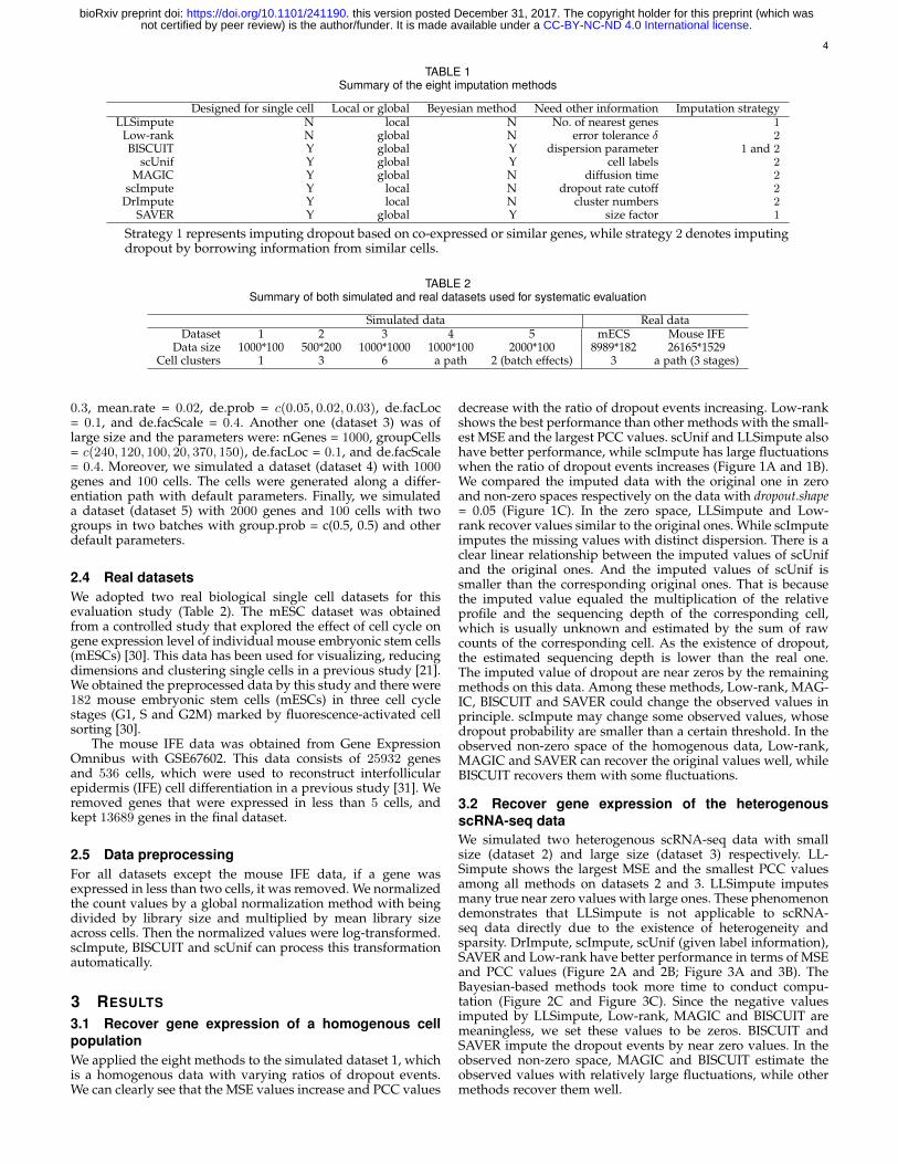
TABLE 1Summary of the eight imputation methods

Designed for single cell Local or global Beyesian method Need other information Imputation strategyLLSimpute N local N No. of nearest genes 1

Low-rank N global N error tolerance δ 2BISCUIT Y global Y dispersion parameter 1 and 2

scUnif Y global Y cell labels 2MAGIC Y global N diffusion time 2

scImpute Y local N dropout rate cutoff 2DrImpute Y local N cluster numbers 2

SAVER Y global Y size factor 1

Strategy 1 represents imputing dropout based on co-expressed or similar genes, while strategy 2 denotes imputingdropout by borrowing information from similar cells.

TABLE 2Summary of both simulated and real datasets used for systematic evaluation

Simulated data Real dataDataset 1 2 3 4 5 mECS Mouse IFE

Data size 1000*100 500*200 1000*1000 1000*100 2000*100 8989*182 26165*1529Cell clusters 1 3 6 a path 2 (batch effects) 3 a path (3 stages)

0.3, mean.rate = 0.02, de.prob = c(0.05, 0.02, 0.03), de.facLoc= 0.1, and de.facScale = 0.4. Another one (dataset 3) was oflarge size and the parameters were: nGenes = 1000, groupCells= c(240, 120, 100, 20, 370, 150), de.facLoc = 0.1, and de.facScale= 0.4. Moreover, we simulated a dataset (dataset 4) with 1000genes and 100 cells. The cells were generated along a differ-entiation path with default parameters. Finally, we simulateda dataset (dataset 5) with 2000 genes and 100 cells with twogroups in two batches with group.prob = c(0.5, 0.5) and otherdefault parameters.

2.4 Real datasetsWe adopted two real biological single cell datasets for thisevaluation study (Table 2). The mESC dataset was obtainedfrom a controlled study that explored the effect of cell cycle ongene expression level of individual mouse embryonic stem cells(mESCs) [30]. This data has been used for visualizing, reducingdimensions and clustering single cells in a previous study [21].We obtained the preprocessed data by this study and there were182 mouse embryonic stem cells (mESCs) in three cell cyclestages (G1, S and G2M) marked by fluorescence-activated cellsorting [30].

The mouse IFE data was obtained from Gene ExpressionOmnibus with GSE67602. This data consists of 25932 genesand 536 cells, which were used to reconstruct interfollicularepidermis (IFE) cell differentiation in a previous study [31]. Weremoved genes that were expressed in less than 5 cells, andkept 13689 genes in the final dataset.

2.5 Data preprocessingFor all datasets except the mouse IFE data, if a gene wasexpressed in less than two cells, it was removed. We normalizedthe count values by a global normalization method with beingdivided by library size and multiplied by mean library sizeacross cells. Then the normalized values were log-transformed.scImpute, BISCUIT and scUnif can process this transformationautomatically.

3 RESULTS

3.1 Recover gene expression of a homogenous cellpopulationWe applied the eight methods to the simulated dataset 1, whichis a homogenous data with varying ratios of dropout events.We can clearly see that the MSE values increase and PCC values

decrease with the ratio of dropout events increasing. Low-rankshows the best performance than other methods with the small-est MSE and the largest PCC values. scUnif and LLSimpute alsohave better performance, while scImpute has large fluctuationswhen the ratio of dropout events increases (Figure 1A and 1B).We compared the imputed data with the original one in zeroand non-zero spaces respectively on the data with dropout.shape= 0.05 (Figure 1C). In the zero space, LLSimpute and Low-rank recover values similar to the original ones. While scImputeimputes the missing values with distinct dispersion. There is aclear linear relationship between the imputed values of scUnifand the original ones. And the imputed values of scUnif issmaller than the corresponding original ones. That is becausethe imputed value equaled the multiplication of the relativeprofile and the sequencing depth of the corresponding cell,which is usually unknown and estimated by the sum of rawcounts of the corresponding cell. As the existence of dropout,the estimated sequencing depth is lower than the real one.The imputed value of dropout are near zeros by the remainingmethods on this data. Among these methods, Low-rank, MAG-IC, BISCUIT and SAVER could change the observed values inprinciple. scImpute may change some observed values, whosedropout probability are smaller than a certain threshold. In theobserved non-zero space of the homogenous data, Low-rank,MAGIC and SAVER can recover the original values well, whileBISCUIT recovers them with some fluctuations.

3.2 Recover gene expression of the heterogenousscRNA-seq dataWe simulated two heterogenous scRNA-seq data with smallsize (dataset 2) and large size (dataset 3) respectively. LL-Simpute shows the largest MSE and the smallest PCC valuesamong all methods on datasets 2 and 3. LLSimpute imputesmany true near zero values with large ones. These phenomenondemonstrates that LLSimpute is not applicable to scRNA-seq data directly due to the existence of heterogeneity andsparsity. DrImpute, scImpute, scUnif (given label information),SAVER and Low-rank have better performance in terms of MSEand PCC values (Figure 2A and 2B; Figure 3A and 3B). TheBayesian-based methods took more time to conduct compu-tation (Figure 2C and Figure 3C). Since the negative valuesimputed by LLSimpute, Low-rank, MAGIC and BISCUIT aremeaningless, we set these values to be zeros. BISCUIT andSAVER impute the dropout events by near zero values. In theobserved non-zero space, MAGIC and BISCUIT estimate theobserved values with relatively large fluctuations, while othermethods recover them well.

.CC-BY-NC-ND 4.0 International licensenot certified by peer review) is the author/funder. It is made available under aThe copyright holder for this preprint (which wasthis version posted December 31, 2017. . https://doi.org/10.1101/241190doi: bioRxiv preprint

5

C

BA

Fig. 1. Direct evaluation of the eight imputation methods on simulated dataset 1. (A) MSE values varies across various dropout ratios. (B) PCCvalues of all single cell pair computed between the imputed data and the original one. (C) Density plot of the imputed values versus the originalones in the zero space (top) and the observed non-zero space (bottom), respectively.

A B C

D

Fig. 2. Direct evaluation of the eight imputation methods on simulated dataset 2. (A) MSE values of each imputation method. (B) PCC values of allsingle cell pair computed between the imputed data and the original one. (C) Computational time (seconds) of running each imputation method. (D)Density plot of the imputed values versus the original ones in the zero space (top) and the observed non-zero space (bottom), respectively.

.CC-BY-NC-ND 4.0 International licensenot certified by peer review) is the author/funder. It is made available under aThe copyright holder for this preprint (which wasthis version posted December 31, 2017. . https://doi.org/10.1101/241190doi: bioRxiv preprint

6

A B C

D

Fig. 3. Direct evaluation of the eight imputation methods on simulated dataset 3. (A) MSE values of each imputation method. (B) PCC valuesof all single cell pair computed between each cell of the imputed data and the original one. (C) Computational time (seconds) of running eachimputation method. (D) Density plot of the imputed values versus the original ones in the zero space (top) and the observed non-zero space(bottom), respectively.

A

B C D E

F G

Fig. 4. Performance of the eight imputation methods on simulated dataset 5. (A) Density plot of the imputed values versus the original ones in thezero space (top) and the observed non-zero space (bottom), respectively. (B) PCA visualization of the raw data and the original one with groupsrepresented by different colors and batches denoted by different shapes. (C) MSE values of each imputation method. (D) PCC values of all singlecell pair computed between the imputed data and the original one. (E) Computational time (seconds) of running each imputation method. (F)Clustering performance of the eight imputation methods on simulated dataset 5. (G) Performance of detecting DEGs.

.CC-BY-NC-ND 4.0 International licensenot certified by peer review) is the author/funder. It is made available under aThe copyright holder for this preprint (which wasthis version posted December 31, 2017. . https://doi.org/10.1101/241190doi: bioRxiv preprint

7

We also simulated a heterogenous scRNA-seq data (dataset5) with batch effect. By PCA visualizing, we can see that thecells in this raw data are mixed together, while the cells inthe full data are separated due to batch effects. Interestingly,the batch effects are stronger than group effects with the for-mer represented as the first component, while another as thesecond component (Figure 4B). Low-rank performs the beston this data with the largest PCC and smallest MSE values.Both imputation methods recover non-zero values well (Figure4A). This might because that many similar cells were clusteredtogether as illustrated by PCA visualization on the normalizeddata. However, BISCUIT and SAVER might fail to capture batcheffect.

3.3 Imputation methods demonstrate diverse ability inpreserving data structuresProper imputation of dropout values should preserve the un-derlying data structures. We assessed the imputation meth-ods in several indirect ways including dimension reduction,cell-type clustering, DEG detection and pseudotime trajectoryreconstruction. CIDR and ZIFA are two dimension reductionmethods, which can address dropout events directly. Comparedwith CIDR and ZIFA, we visualized the raw data, original dataand imputed data by PCA (Figure 5). Low-rank, scImpute,DrImpute, scUnif and SAVER outperform other methods andare consistent with patterns of real data in the first two PCdimensions. Though ZIFA has more divergent clusters thanother methods, it is far from real data in the low dimensionalspace, which might introduce new noise. As the clusters ofsimulated dataset 3 is not separable in the first two principlecomponents, we also visualized dataset 3 with tSNE. Low-rank,scImpute, DrImpute, scUnif and SAVER still discover differentclusters. Interestingly, Low-rank gets the most similar structurewith that in the real data in the low-dimensional space (Figure6B).

Identifying cell subpopulations is a key application ofscRNA-seq and some clustering methods may fail due to theexistence of dropout events. SC3 and SIMLR have been devel-oped for clustering scRNA-seq data, and both of them do notaddress dropout events directly. We evaluated the effectivenessof these imputation methods with impacts on the clusteringperformance of SC3, SIMLR and k-means with the first twotSNE dimensions (tSNE+kmeans). The clustering performancewas assessed by the normalized mutual information (NMI)[32], Jaccard index, purity, and adjusted rand index (ARI). SC3shows better performance than SIMLR and tSNE+kmeans onsimulated datasets 2 and 3. As the first two tSNE componentscapture little information of the simulated dataset 2 (Figure6A), tSNE+kmeans has a worse clustering performance. Low-rank, scImpute, DrImpute, scUnif and SAVER improve theclustering performance of SC3 on simulated datasets 2 and3. In the simulated dataset 2, scUnif and scImpute have thebest performance, but scUnif needs cell labels information inadvance. Low-rank and DrImpute also have better performance(Figure 7). In the large simulated dataset 3, Low-rank, scImpute,DrImpute, scUnif and SAVER also enhance the clustering per-formance of SIMLR and tSNE+kmeans. Interestingly, SIMLRand tSNE+kmeans applied to the imputed data by Low-rank,scImpute, DrImpute, scUnif and SAVER have better perfor-mance than CIDR (Figure 8). However, CIDR outperforms bothof these clustering methods even on the real data on simulateddataset 5 (Figure 4F).

To evaluate the robustness of imputation methods, wedown-sampled 50 cells at random on simulated dataset 2 withfive repetitions. We clustered the down-sampled cells withor without imputing the dropout events by SC3, SIMLR andtSNE+kmeans respectively. The clustering performance showthat scUnif has the best robustness, while scImpute is not asgood as that of using all cells (Figure 9).

A

B

Fig. 5. PCA visualization of the reduced dimensions of the eight imputa-tion methods on simulated datasets 2 (A) and 3 (B).

A

B

Fig. 6. tSNE visualization of the reduced dimensions of the eight impu-tation methods on simulated datasets 2 (A) and 3 (B).

Detecting DEGs is also an important downstream analy-sis of scRNA-seq data. We assessed the recovery power ofimputation methods in identifying DEGs from the raw data.We can see that MAST has the worst performance comparedto other methods in these two simulated datasets 2 and 3.scImpute, DrImpute and scUnif slightly enhance the perfor-mance of edgeR in detecting DEGs, which are better than MASTand SCDE. edgeR has similar performance on raw data withLow-rank, BISCUIT and SAVER on the imputed data. SCDEdemonstrate the best AUPR value than other methods (Figure10). Moreover, the imputation methods have no advantages onimproving the performance of edgeR on the simulated dataset3 (Figure 11). DrImpute and BISCUIT have better performance

.CC-BY-NC-ND 4.0 International licensenot certified by peer review) is the author/funder. It is made available under aThe copyright holder for this preprint (which wasthis version posted December 31, 2017. . https://doi.org/10.1101/241190doi: bioRxiv preprint

8

Fig. 7. Clustering performance of the eight imputation methods on simulated dataset 2.

Fig. 8. Clustering performance of the eight imputation methods on simulated dataset 3.

than other methods, while LLSimpute and MAGIC have theworst performance on simulation dataset 3. Interestingly, im-putation methods except MAGIC and BISCUIT enhance thesensitivity of edgeR in detecting DEGs, while these methodshave smaller AUPR values than those of MAGIC and BISCUIT(Figure 4G).

scRNA sequencing has already shown its power in re-constructing developmental trajectories [33]. We employed thesimulated dataset 4 with a path and no branches to compare theimpacts of imputation methods on inferring pseudotime order.As LLSimput imputed data does not satisfy the requirementof Monocle 2, we did not show the pseudotemporal order ofit. scImpute and SAVER have more consistent trajectories withthat constructed in the original data (Figure 12). The measur-

able indicator of order conformity (named as order correlation)is defined as C/(Nc + C), where C represents the numberof similar orders between the pseudotime and gold standardorders, and Nc denotes the number of dissimilar orders. scIm-pute, DrImpute and SAVER improve the power of Monocle 2in ordering cells along a trajectory in terms of this index. Wedown-sampled 50 cells randomly for five repetitions, imputedthem by these imputation methods and inferred trajectorieswith or without imputing the dropout events. We can see thatLow-rank has the largest order correlations than those of othermethods, enhancing the power of Monocle 2 by imputing thedropout events. Moreover, MAGIC has the worse performancewhen we randomly selected some cells to infer a trajectory.

In summary, Low-rank, scImpute, DrImpute, scUnif and

.CC-BY-NC-ND 4.0 International licensenot certified by peer review) is the author/funder. It is made available under aThe copyright holder for this preprint (which wasthis version posted December 31, 2017. . https://doi.org/10.1101/241190doi: bioRxiv preprint

9

Fig. 9. Clustering performance of the eight imputation methods on the down-sampled cells of simulated dataset 2.

A

B

Fig. 10. Performance of detecting DEGs on simulated dataset 2.

SAVER have better performance in dimension reduction andcell clustering, which are even better than CIDR. scImpute,DrImpute and SAVER improves the performance of Monocle2 in reconstructing pseudotime. However, these imputationmethods have no significant improvement for edgeR in de-tecting DEGs. Only scImpute, DrImpute and scUnif slightlyenhance this performance on simulated dataset 2.

3.4 Imputation methods provide more potential DEGsIn the mECS real data, the 182 mESC cells consist of 59 cells inG1 phase, 58 cells in S phase and 65 cells in G2/M phase. Firstly,BISCUIT and SAVER impute zeros with near zero values, whileLLSimpute and scImpute impute zeros with relatively largevalues. We compared true values with recovered ones by Low-rank, MAGIC, BISCUIT and SAVER, which will change thevalues in the observed space in principle (Figure 13B). Low-rank and SAVER recover the observed values well, while MAG-

A

B

Fig. 11. Performance of detecting DEGs on simulated dataset 3.

IC and BISCUIT change the observed ones in some degree.However, MAGIC improves the clustering performance of SC3.BISCUIT enhances the power of SC3 in clustering slightly.tSNE+kmeans has better clustering performance on DrImputeimputed data than on the raw data, and even better than CIDR,which addresses dropout events directly. edgeR on LLSimputeimputed data tends to treat each genes as a DEG, which isfallacious (Figure 13D). There are 332 DEGs by SCDE withq-value < 0.05, which are included in the DEG set of edgeRon Low-rank imputed data. We downloaded mouse cell cyclestage-specific maker genes from a previous study [31], whichincludes 43 (31) and 54 (51) marker genes of G1/S and G2/M(in the processed data) respectively.

The DEGs of SCDE is significantly enriched with the G1/Sand G2/M marker genes using Fisher’s exact test with FDR< 0.05. However, only PLK1 is regarded as DEG by SCDEwith FDR < 0.01. The activity of PLK1 is indeed regulatedby cell cycle, which is in low activity during interphase but

.CC-BY-NC-ND 4.0 International licensenot certified by peer review) is the author/funder. It is made available under aThe copyright holder for this preprint (which wasthis version posted December 31, 2017. . https://doi.org/10.1101/241190doi: bioRxiv preprint

10

A

C

D

B

Fig. 12. Performance of reconstructing pseudotime order of scRNA-seq data using imputation methods or not on simulated dataset 4. (A)Visualization of the inferred trajectory using each method. Each dot represents a cell. Cells with higher values are in more differentiated states. (B)Order correlation of pseudotime inferred from Monocle 2 on the raw data, original data, and imputed data with golden standard pseudotime. (C)Computational time (seconds) of running each imputation method. (D) Boxplot of order correlation of five repetitions with 50 cells.

high during mitosis [34]. MAGIC enhances the enrichment ofmarker genes with higher fold-changes (Figure 13E). Thereare six G2/M marker genes detected by eageR on MAGICimputed data but ignored by SCDE. These genes indeed havehigher count level in G2 cells recovered by MAGIC (Figure 14).The Bayesian-based imputation methods are still more time-consuming than other methods (Figure 13F).

Fig. 14. Violinplot of the imputed count values of G2/M marker genes,which are detected by edgeR using MAGIC imputed data but ignored bySCDE.

3.5 Imputation methods improve the reconstruction ofepidermal differentiation processThe great regenerative capacity of murine epidermis and itsappendages enable it to be an invaluable model system for

stem cell biology. Recently, the cellular heterogeneity of theadult mouse epidermis has been examined using scRNA-seq.The pseudotemporal order of IFE cells has been obtained bya minimum spanning tree-based method in tSNE space [31].Applied imputation methods to this dataset, we can see thatBISCUIT still imputes zeros with near zero values in this data.MAGIC and SAVER recover non-zero values with large devi-ation, while BISCUIT recover non-zero values well, indicatingthat there is small technical variation detected by BISCUIT inthis data (Figure 15A and 15B).

We inferred the pseudotime of individual cells by Monocle1 [23] and Monocle 2 [24] on the raw data and imputeddata respectively. The transcribed repetitive elements (i.e., genename stated with ”r ”) were removed from the gene list. Thetrajectory reconstructed on the raw data and imputed databy these imputation methods except Low-rank and scUnif aremore consistent with the one inferred by the spanning treemodel visually [31]. Based on the order correlation, MAGIC,BISCUIT and SAVER preserve the differentiation direction well,which starts from IFE basal cells to IFE differentiated cells, thenarrives at IFE keratinized layer (Figure 15D). However, any im-putation methods cannot enhance the performance of Monocle2 due to its efficiency. Interestingly, Monocle 1 is not as effectiveas Monocle 2 on the raw data. SAVER, Low-rank, scUnif andscImpute improve the ability of Monocle 1 clearly (Figure 15E).Therefore, the impact of imputing dropout events may rely onthe downstream analysis method. MAGIC and BISCUIT havemore reliable IFE differentiation process as the pseudotimeorder of the known basal maker (Krt14), mature marker (Krt10),terminally differentiated cell stage marker (Lor) and a transientmarker (Mt4) gradually vary along the trajectory within eachcluster than those of other imputation methods (Figure 16).

.CC-BY-NC-ND 4.0 International licensenot certified by peer review) is the author/funder. It is made available under aThe copyright holder for this preprint (which wasthis version posted December 31, 2017. . https://doi.org/10.1101/241190doi: bioRxiv preprint

11

A

FE

C

Cutoff = 0.05

Cutoff = 0.01

D

B

Low-rank MAGIC BISCUIT SAVER

Imputed value

Tru

e v

alu

e

Fig. 13. Performance of the eight imputation methods on the mESC data. (A) Boxplot of the imputed values of each method on the zero space.(B) Density plot of the recovered values versus original ones in the observed non-zero space using Low-rank, MAGIC, BISCUIT and SAVER withy-axis representing log-transformed observed non-zero values and x-axis denoting log-transformed recovered values. (C) Clustering performanceof CIDR on raw data and SC3, SIMLR, tSNE+k-means on raw data and imputed data in terms of NMI, Jaccard, Purity and ARI respectively. (D)Heatmap of -log10(q) value of MAST, SCDE on raw data and edgeR on raw and imputed data for detecting DEGs. (E) Barplot of -log10(q) andfold-change of Fishers exact test on the enrichment analysis of 82 G1/S, G2/M maker genes. (F) Computational time (seconds) of running eachimputation method.

4 CONCLUSION AND DISCUSSION

The main goal of this study is to provide a straightforward andthorough comparison on the imputation methods for scRNA-seq data. We systematically evaluated eight imputation meth-ods including two for general incomplete data and six speciallydesigned for scRNA-seq data from multiple angles. We summa-rized the impacts of eight imputation methods on the simulatedand real datasets (Table 3). Firstly, LLSimpute designed forthe bulk-RNAseq data performs well in a homogenous cellpopulation, but it fails when the data shows large heterogeneityand sparsity, which are two key characteristics of scRNA-seqdata. Low-rank also performs well in datasets 1 and 5. It isnot affected by batch effect applying to all genes. Secondly,scImpute and DrImpute recover the data well in simulateddatasets. However, they fail on the data with less collinearity(e.g., mESC data). Thirdly, simulation study illustrates that BIS-CUIT and SAVER tend to impute the dropout events with nearzero values. MAGIC and BISCUIT recover non-zero values withlarge fluctuations. MAGIC shows better performance to helpto detect biomarkers in mouse mESC data. MAGIC designedbased on a Markov affinity-based graph could capture the grad-ual variation of genes. Therefore, it enhances the performanceof Monocle 2 to reconstruct marker genes expression change

along differentiation process. However, it fails to improve theability of Monocle 1. These results demonstrate that the impactsof imputing dropout events on downstream analysis depend onthe analysis methods.

Extensive studies highlight that there is no one methodperforms the best in all situations. Current methods still havesome defects such as scalability, robustness and applicabilityin some situations. With the rapid generation of large-scalescRNA-seq data, imputation of dropout events is becoming abasic and routine step in scRNA-seq data analysis. Therefore,efficient methods and powerful tools for imputation are ur-gently needed at present. Moreover, efficient information fromgenes such as co-expressed networks should be used in futurestudies.

ACKNOWLEDGMENT

Shihua Zhang is the corresponding author of this paper. Thiswork has been supported by the National Natural ScienceFoundation of China [No. 61422309, 61379092, 61621003 and11661141019]; the Strategic Priority Research Program of theChinese Academy of Sciences (CAS) [No. XDB13040600], theKey Research Program of the Chinese Academy of Sciences

.CC-BY-NC-ND 4.0 International licensenot certified by peer review) is the author/funder. It is made available under aThe copyright holder for this preprint (which wasthis version posted December 31, 2017. . https://doi.org/10.1101/241190doi: bioRxiv preprint

12

A B

C

Low-rank MAGIC BISCUIT SAVER

D E FMonocle 2 Monocle 1

Imputed value

Tru

e v

alu

e

Fig. 15. Pseudotime reconstruction of IFE data. (A) Boxplot of the log-transformed imputed values of the eight imputation methods on the zerospace. (B) Density plot of the recovered values versus the original ones in the observed non-zero space using Low-rank, MAGIC, BISCUIT andSAVER with y-axis representing log-transformed true values and x-axis denoting log-transformed recovered values. (C) Visualization of the inferredtrajectory of each method. Each dot represents a cell. Cells with higher values are in more differentiated states. (D) Order correlation of pseudotimeinferred from Monocle 2 on the raw data and imputed data with golden standard pseudotime. (E) Order correlation of pseudotime inferred fromMonocle 1 on the raw data and imputed data with golden standard pseudotime. (F) Computational time (seconds) of running each imputationmethod.

[No. KFZD-SW-219] and CAS Frontier Science Research KeyProject for Top Young Scientist [No. QYZDB-SSW-SYS008].

REFERENCES[1] F. Tang, C. Barbacioru, Y. Wang, E. Nordman, C. Lee, N. Xu,

X. Wang, J. Bodeau, B. B. Tuch, A. Siddiqui et al., “mrna-seq whole-transcriptome analysis of a single cell,” Nat. Med., vol. 6, no. 5, pp.377–382, 2009.

[2] G. Kelsey, O. Stegle, and W. Reik, “Single-cell epigenomics:Recording the past and predicting the future,” Science, vol. 358,no. 6359, pp. 69–75, 2017.

[3] M. J. Stubbington, O. Rozenblatt-Rosen, A. Regev, and S. A.Teichmann, “Single-cell transcriptomics to explore the immunesystem in health and disease,” Science, vol. 358, no. 6359, pp. 58–63,2017.

[4] P. V. Kharchenko, L. Silberstein, and D. T. Scadden, “Bayesianapproach to single-cell differential expression analysis,” Nat. Med.,vol. 11, no. 7, pp. 740–742, 2014.

[5] Z. Miao and X. Zhang, “Desingle: A new method for single-cell differentially expressed genes detection and classification,”bioRxiv, p. 173997, 2017.

[6] H. Kim, G. H. Golub, and H. Park, “Missing value estimation fordna microarray gene expression data: local least squares imputa-tion,” Bioinformatics, vol. 21, no. 2, pp. 187–198, 2004.

[7] T. Aittokallio, “Dealing with missing values in large-scale studies:microarray data imputation and beyond,” Brief Bioinform., vol. 11,no. 2, pp. 253–264, 2009.

[8] K. Moorthy, M. Saberi Mohamad, and S. Deris, “A review on miss-ing value imputation algorithms for microarray gene expressiondata,” Curr Bioinform., vol. 9, no. 1, pp. 18–22, 2014.

[9] C. Chen, B. He, and X. Yuan, “Matrix completion via an alternatingdirection method,” IMA J. Numer. Anal., vol. 32, no. 1, pp. 227–245,2012.

[10] E. J. Candes and B. Recht, “Exact matrix completion via convexoptimization,” Found. Comput. Math., vol. 9, no. 6, p. 717, 2009.

[11] S. Prabhakaran, E. Azizi, A. Carr, and D. Peer, “Dirichlet processmixture model for correcting technical variation in single-cell geneexpression data,” Proc. 33nd Int. Conf. Mach. Learn., ICML, pp.1070–1079, 2016.

[12] L. Zhu, J. Lei, B. Devlin, and K. Roeder, “A unified statisticalframework for single cell and bulk rna sequencing data,” bioRxiv,p. 206532, 2017.

[13] D. van Dijk, J. Nainys, R. Sharma, P. Kathail, A. J. Carr, K. R. Moon,L. Mazutis, G. Wolf, S. Krishnaswamy, and D. Pe’er, “Magic: Adiffusion-based imputation method reveals gene-gene interactionsin single-cell rna-sequencing data,” BioRxiv, p. 111591, 2017.

[14] W. V. Li and J. J. Li, “scimpute: accurate and robust imputation forsingle cell rna-seq data,” bioRxiv, p. 141598, 2017.

.CC-BY-NC-ND 4.0 International licensenot certified by peer review) is the author/funder. It is made available under aThe copyright holder for this preprint (which wasthis version posted December 31, 2017. . https://doi.org/10.1101/241190doi: bioRxiv preprint

13

Fig. 16. Validation of pseudotemporal ordering of IFE cells with four marker genes Krt14, Krt10, Lor and Mt4 using the raw data and imputed databy Monocle respectively. Each dot represents a cell. The IFE basal cells, IFE differentiated cells and IFE keratinized layer are denoted by blue,green and red colors respectively. The gene expression of these markers were fitted with cubic smoothing splines.

[15] R. Tibshirani, “Regression shrinkage and selection via the lasso,”J. Royal Statistical Soc. B, pp. 267–288, 1996.

[16] V. Y. Kiselev, K. Kirschner, M. T. Schaub, T. Andrews, A. Yiu,T. Chandra, K. N. Natarajan, W. Reik, M. Barahona, A. R. Greenet al., “Sc3: consensus clustering of single-cell rna-seq data,” Nat.Med., 2017.

[17] I.-Y. Kwak, W. Gong, N. Koyano-Nakagawa, and D. Garry, “Drim-pute: Imputing dropout events in single cell rna sequencing data,”bioRxiv, p. 181479, 2017.

[18] M. Huang, J. Wang, E. Torre, H. Dueck, S. Shaffer, R. Bonasio,J. Murray, A. Raj, M. Li, and N. R. Zhang, “Gene expressionrecovery for single cell rna sequencing,” bioRxiv, p. 138677, 2017.

[19] E. Pierson and C. Yau, “Zifa: Dimensionality reduction for zero-inflated single-cell gene expression analysis,” Genome Biol, vol. 16,no. 1, p. 241, 2015.

[20] P. Lin, M. Troup, and J. W. Ho, “Cidr: Ultrafast and accurate clus-tering through imputation for single-cell rna-seq data,” GenomeBiol, vol. 18, no. 1, p. 59, 2017.

[21] B. Wang, J. Zhu, E. Pierson, D. Ramazzotti, and S. Batzoglou,“Visualization and analysis of single-cell rna-seq data by kernel-based similarity learning,” Nat. Med., vol. 14, no. 4, pp. 414–416,

2017.[22] G. Finak, A. McDavid, M. Yajima, J. Deng, V. Gersuk, A. K. Shalek,

C. K. Slichter, H. W. Miller, M. J. McElrath, M. Prlic et al., “Mast: aflexible statistical framework for assessing transcriptional changesand characterizing heterogeneity in single-cell rna sequencingdata,” Genome Biol, vol. 16, no. 1, p. 278, 2015.

[23] C. Trapnell, D. Cacchiarelli, J. Grimsby, P. Pokharel, S. Li,M. Morse, N. J. Lennon, K. J. Livak, T. S. Mikkelsen, and J. L. Rinn,“The dynamics and regulators of cell fate decisions are revealed bypseudotemporal ordering of single cells,” Nat. Biotechnol., vol. 32,no. 4, pp. 381–386, 2014.

[24] X. Qiu, Q. Mao, Y. Tang, L. Wang, R. Chawla, H. A. Pliner, andC. Trapnell, “Reversed graph embedding resolves complex single-cell trajectories,” Nat. Med., vol. 14, no. 10, pp. 979–982, 2017.

[25] I. T. Jolliffe, “Principal component analysis and factor analysis,”pp. 115–128, 1986.

[26] L. v. d. Maaten and G. Hinton, “Visualizing data using t-sne,” J.Mach. Learn Res., vol. 9, no. Nov, pp. 2579–2605, 2008.

[27] M. D. Robinson, D. J. McCarthy, and G. K. Smyth, “edger: abioconductor package for differential expression analysis of digitalgene expression data,” Bioinformatics, vol. 26, no. 1, pp. 139–140,

.CC-BY-NC-ND 4.0 International licensenot certified by peer review) is the author/funder. It is made available under aThe copyright holder for this preprint (which wasthis version posted December 31, 2017. . https://doi.org/10.1101/241190doi: bioRxiv preprint

14

TABLE 3Summary of systematic evaluation of the eight methods using both simulated and real datasets

Dataset Evaluation strategies LLSimpute Low-rank MAGIC scImpute DrImpute BISCUIT scUnif SAVERDataset 1 PCC 2a 1a 7b 4a 5a 8b 3a 6aDataset 2 PCC 8c 5a 6b 2a 1a 7b 3a 4a

Clustering 7c 3a 8c 2a 4a 6c 1a 5aRobustness 5a 3a 7c 2a 6a 8c 1a 4aDE 8c 6b 7c 3a 1a 5b 2a 4b

Dataset 3 PCC 8c 5a 6b 2a 1a 7b 3a 4aClustering 8c 4a 7c 3a 2a 6b 5a 1aDE 8c 6c 7c 4b 1b 5c 2b 3b

Dataset 4 PCC 8b 5a 6a 2a 1a 7b 3a 4aPseudotime 8c 4b 7c 1a 2a 6b 5b 3aRobustness 8c 1a 7c 3b 5c 6c 4b 2b

Dataset 5 PCC 2a 1a 7b 4a 5a 8b 3a 6bClustering 1a 6b 4b 3a 5b 8b 2a 7bDE 2a 1a 7b 4a 5a 8b 3a 6a

mESC Clustering 8c 5c 1a 4c 3c 2a 7c 6cBiomarker enrichment 6b 4b 1a 8c 7c 3a 2a 5b

IFE Monocle 1 8c 2a 7b 4a 5b 6b 3a 1aMonocle 2 8c 7c 3b 6c 4c 1b 5c 2b

Each entry consists of a combination of an integer number in 1, 2, · · · , 8 and a letter in a, b, c. The numberrepresents the performance rank of each method for a corresponding strategy. Rank 1 and 8 represent the best andworst performance respectively. The letter represents the improvement degree compared to the performance on theraw data: significant increase, no change and significant decrease.

2010.[28] L. Zappia, B. Phipson, and A. Oshlack, “Splatter: simulation of

single-cell rna sequencing data,” Genome Biol, vol. 18, no. 1, p. 174,2017.

[29] B. Vieth, C. Ziegenhain, S. Parekh, W. Enard, and I. Hellmann,“powsimr: Power analysis for bulk and single cell rna-seq experi-ments,” Bioinformatics, vol. 33, no. 21, pp. 3486–3488, 2017.

[30] F. Buettner, K. N. Natarajan, F. P. Casale, V. Proserpio, A. Scial-done, F. J. Theis, S. A. Teichmann, J. C. Marioni, and O. Stegle,“Computational analysis of cell-to-cell heterogeneity in single-cellrna-sequencing data reveals hidden subpopulations of cells,” Nat.Biotechnol., vol. 33, no. 2, pp. 155–160, 2015.

[31] S. Joost, A. Zeisel, T. Jacob, X. Sun, G. La Manno, P. Lonnerberg,S. Linnarsson, and M. Kasper, “Single-cell transcriptomics revealsthat differentiation and spatial signatures shape epidermal andhair follicle heterogeneity,” Cell Sys, vol. 3, no. 3, pp. 221–237, 2016.

[32] I. H. Witten, E. Frank, M. A. Hall, and C. J. Pal, Data Mining:Practical machine learning tools and techniques. Morgan Kaufmann,2016.

[33] S. C. Bendall, K. L. Davis, E.-a. D. Amir, M. D. Tadmor, E. F.Simonds, T. J. Chen, D. K. Shenfeld, G. P. Nolan, and D. Peer,“Single-cell trajectory detection uncovers progression and regula-tory coordination in human b cell development,” Cell, vol. 157,no. 3, pp. 714–725, 2014.

[34] R. M. Golsteyn, K. E. Mundt, A. M. Fry, and E. A. Nigg, “Cellcycle regulation of the activity and subcellular localization of plk1,a human protein kinase implicated in mitotic spindle function.” J.Cell Biol., vol. 129, no. 6, pp. 1617–1628, 1995.

.CC-BY-NC-ND 4.0 International licensenot certified by peer review) is the author/funder. It is made available under aThe copyright holder for this preprint (which wasthis version posted December 31, 2017. . https://doi.org/10.1101/241190doi: bioRxiv preprint