Comparison between Staggered and Unstaggered Finite ... · Comparison between Staggered and...

Journal of Computational Physics161,379–400 (2000)

doi:10.1006/jcph.2000.6460, available online at http://www.idealibrary.com on

Comparison between Staggered andUnstaggered Finite-Difference Time-Domain

Grids for Few-Cycle Temporal OpticalSoliton Propagation

L. Gilles,∗,† S. C. Hagness,∗ and L. Vazquez†∗Department of Electrical and Computer Engineering, University of Wisconsin, 1415 Engineering Drive,

Madison, Wisconsin 53706; and†Departamento de Matematica Aplicada, Escuela Superior deInformatica, Universidad Complutense, E-28040 Madrid, SpainE-mail: [email protected] and [email protected]

Received July 21, 1999; revised January 19, 2000

The auxiliary-differential-equation formulation of the finite-difference time-domain method has become a powerful tool for modeling electromagnetic wavepropagation in linear and nonlinear dispersive media. In the first part of this pa-per, we compare the stability and accuracy of second- and fourth-order-accuratespatial central discretizations on staggered grids with a third-order-accurate spatialdiscretization on an unstaggered grid, combined with a second-order leapfrog timeintegration scheme for modeling linear dispersive phenomena in a one-dimensionalsingle-resonance Lorentz medium. We use on the unstaggered grid the NS2 schemeintroduced by Y. Liu, which combines forward and backward differencing for thespatial derivatives. Phase and attenuation errors are determined analytically acrossthe entire frequency band of the low-loss single-resonance Lorentz model. In thesecond part of the paper, we compare the use of one-dimensional staggered and un-staggered grids for modeling the transient evolution of few-cycle optical localizedpulses in a dispersive Lorentz medium with a delayed third-order nonlinearity. Thefocus of the study is on the decay of higher-order solitons under the combined actionof dispersion, self-phase modulation, self-steepening, and stimulated Raman scatter-ing. Numerical results from the simulations on the unstaggered and staggered gridsare in excellent agreement. This study demonstrates the accuracy of the unstaggeredscheme augmented with a linear/nonlinear dispersive media formulation for temporalsoliton propagation. c© 2000 Academic Press

Key Words:finite-difference time-domain methods; Maxwell’s equations; stag-gered grids; unstaggered grids; material dispersion; nonlinear optics; optical solitons.

379

0021-9991/00 $35.00Copyright c© 2000 by Academic Press

All rights of reproduction in any form reserved.

380 GILLES, HAGNESS, AND VAZQUEZ

1. INTRODUCTION

Finite-difference time-domain (FDTD) modeling of electromagnetic pulse propagation innonlinear optical materials has recently gained much attention [1]. The auxiliary-differential-equation (ADE) formulation, initially developed for linear dispersive mate-rials [2], is currently the most commonly used approach for incorporating the nonlinearrelationship between the polarization vector and the electric field into the FDTD Maxwell’sequation solver [3, 4]. This modeling capability has been applied to a variety of second-and third-order nonlinear phenomena, including temporal and spatial soliton propagation[3, 5, 6], self-focusing of optical beams [4], scattering from linear–nonlinear interfaces [7],pulse propagation through nonlinear corrugated waveguides [8], pulse-selective behaviorin nonlinear Fabry–Perot cavities [9], and second-harmonic generation in nonlinear wave-guides [10].

Stability, numerical dispersion, and artificial dissipation are factors in FDTD-ADE mod-eling that must be accounted for to understand the algorithm’s operation and its accuracylimits. Petropoulos [11], Younget al. [12], and Cummer [13] have analyzed the stabilityand numerical dispersion relations for second-order-accurate central differencing schemesinvolving the Yee [14] staggered grid where the electric and magnetic field vectors areinterleaved. Using a different approach, Petropoulos [15] determined the grid resolution,in terms of a fixed total computation time and desired phase error, for both second- andfourth-order Yee schemes in two dimensions for free-space propagation.

In the past, staggered grids have usually been preferred over unstaggered grids for thefollowing reasons. On an unstaggered grid, the electric and magnetic field vectors are placedon the same primary grid and all vector field components are colocated. Central differenc-ing on an unstaggered grid can lead to undesirable numerical oscillations due to odd–evendecoupling [16]. Moreover, the standard unstaggered scheme produces a relative total nu-merical phase velocity error four times greater than the staggered scheme due to the widerstencil. Despite these problems, the unstaggered grid with its inherently colocated electricfield vector components offers several advantages specific to the modeling of optical wavephenomena. For example, unstaggered schemes enable the use of a moving window coordi-nate frame for tracking long-distance optical pulse propagation [17, 18]. Most importantly,the use of a grid with colocated electric field vector components is essential for efficient andaccurate modeling of nonlinear optical wave propagation in two or three dimensions. Thereason for this is the fact that the presence of the nonlinearity requires calculating higher-order powers of the electric field intensity at a given point in space at every time step. Ifthe electric field vector components are not colocated, as is the case with the staggeredYee scheme, then the field intensity at a given point in space must be interpolated from theknown field components centered around that point. This interpolation is costly in terms ofcomputational efficiency and accuracy, and can be avoided altogether if the electric fieldvectors are colocated.1

Liu [19] suggested an interesting way to combine the desirable properties of the staggeredand unstaggered grids. His approach uses noncentral differencing based on a combination

1 We note that the unstaggered grid is not the only option for colocating the electric field vector components.For example, colocated staggered grids have been proposed where the electric and magnetic field vectors areplaced on dual grids but where all components of any given field vector are colocated [19]. We do not considerthose schemes here because they require about twice the number of operations [19]. Furthermore, a 1D version ofsuch a scheme does not exist.

COMPARISON OF FDTD GRIDS FOR OPTICAL SOLITON PROPAGATION 381

of forward and backward differencing (FD/BD) for the spatial derivatives on an unstaggeredgrid. In this manner, the even–odd coupling is preserved even though the fields are colo-cated; thus spurious oscillations are avoided. The methods referred to as NS2 and NS3 in[19] (NS meaning “nonsymmetric”) are finite-difference (FD) discretizations of first-orderderivatives in Maxwell’s curl equations with third- and first-order accuracy, respectively. In[19], numerical experiments supported the claim that the NS2 and NS3 schemes targetedfourth- and sixth-order accuracy in space, respectively, as is the case for the correspondingwave-equation systems containing second-order derivatives. However, as shown recentlyby Driscoll and Fornberg [20], such noncentral differencing only retains the accuracy ofthe first-order derivatives.

In this paper, we compare the Yee (staggered) and Liu NS2 (unstaggered) schemes formodeling pulse propagation in linear and nonlinear dispersive media. Time integration isperformed for both grid configurations in the usual second-order leapfrog manner. Second-and fourth-order spatial accuracy is considered on the staggered grids and third-orderspatial accuracy on the unstaggered grid. Therefore, we denote the various schemes as Y22,Y24, and NS2. We do not include the NS3 method in this analysis as it is only first-orderaccurate and therefore unable to capture the correct physics in the medium absorption band.

First, we compare the stability and accuracy of the Y22, Y24, and NS2 FDTD-ADEschemes for alinear single-resonance Lorentz medium. We conduct a Von Neumann analy-sis of each approach in order to determine stability criteria. Using CFL numbers below andat the stability limit, we investigate phase and attenuation errors across the entire frequencyband of the Lorentz model. Second, we compare the results from the two grid arrangementsin modeling the transient evolution of few-cycle optical localized pulses in a Lorentz dis-persive medium withnonlinearthird-order delayed response modeling Raman scattering.Since the Courant limit for the nonlinear algorithm is not known, the nonlinear algorithmswere run below their linear CFL limit.

The focus of the numerical experiments is on the decay of linearly polarized fundamen-tal and second-order bright soliton pulses due to the combined action third-order disper-sion (TOD), self-phase modulation (SPM), self-steepening (SS), and Raman self-scattering(RSS) [21]. These numerical experiments provide a rigorous test bed for comparing theaccuracy of the staggered and unstaggered FDTD-ADE schemes. Higher-order solitonsare nonlinear superpositions of single solitons with no binding energy. In the presence ofsmall perturbations, they decay and split into their single-soliton constituents. Their decayhas been investigated for a variety of cases, including the effects of TOD, SS, and SRS[22, 23]. The dynamics of their decay is very rich due to nonlinear interactions amongthe multiple single constitutive solitons. Striking examples include the breakup of higher-order soliton pulses under the action of two-photon absorption (TPA) and the complicatedevolution of these solitons under periodic amplification. Higher-order solitons have re-ceived less attention than fundamental solitons mainly because they are not as robust.However, they exhibit important features like periodic beating [24] due to phase interfer-ence among the constitutive solitons, and therefore offer potential applications in switchingdevices.

2. THE NONLINEAR MAXWELL’S EQUATIONS

Maxwell’s equations describing the propagation of light in nonlinear dispersive envi-ronments with no free charges are expressed in terms of (E, H) the electric and magnetic


fields, respectively, and (D, B) the corresponding electric and magnetic flux densities,as

∇ × E = − ∂∂t

B,(1)

∇ × H = ∂

∂tD.

For nonmagnetic media the constitutive relations take the form

B = µ0H,(2)

D = ε0PTOT,

whereµ0, ε0, are the free space permeability and permittivity. The total polarization

PTOT = P+ PNL (3)

is related to the electric field through the relations

P =∫ t

−∞χ(1)(t − t1)E(t1) dt1, (4)

PNL = E(t)∫ t

−∞χ(3)(t − t1)‖E(t1)‖2 dt1. (5)

Here, for simplicity, we have assumed [27] (i) axially symmetric and isotropic environmentsso that the second-order susceptibility tensorχ(2) is identically zero, (ii)χ(1)=χ(1)yy =χ(1)zz , (iii) χ(3)=χ(3)yyyy=χ(3)zzzz, and (iv) simplification of the third-order susceptibility into asingle nonlinear time convolution involving the field intensity. The susceptibilities can bedecomposed into their instantaneous background and residual parts

χ(1)(t) = ε∞δ(t)+ χ(1)R (t), (6)

χ(3)(t) = a(1− θ)δ(t)+ χ(3)R (t), (7)

whereε∞ is the infinite frequency permittivity,χ(1)R andχ(3)R are the residual susceptibilities,a is the third-order coupling constant, andθ parameterizes the relative strength of theinstantaneous electronic Kerr and residual Raman molecular vibrational responses. Thisdecomposition yields

P = ε∞E+Φ, (8)

PNL = a(1− θ)‖E‖2E+ΦNL, (9)

whereΦ,ΦNL are the residual linear and nonlinear polarizations,

Φ(t) =∫ t

−∞χ(1)R (t − t1)E(t1) dt1 =

∫ ∞0χ(1)R (t1)E(t − t1) dt1,

(10)ΦNL(t) = aθQE,


Q =∫ t

−∞χ(3)R (t − t1)‖E(t1)‖2 dt1. (11)

Q describes the natural molecular vibrations within the dielectric material with frequencymany orders of magnitude less than the optical wave frequency, responding to the fieldintensity. The total third-order nonlinear polarizationPNL reduces to the instantaneousintensity-dependent Kerr response in the limitθ → 0.

In terms of the temporal Fourier transform

E(t) = 1

2π

∫ ∞−∞

E(ω) exp(iωt) dω,

(12)

E(ω) =∫ ∞−∞

E(t) exp(−iωt) dt,

the residual kernel functionsχ(1)R , χ(3)R are modeled by single-resonance Lorentz dipole

oscillators (second-order filters):

χ(1)R (ω) = β1ω

21

ω21 + 2i γω − ω2

,

(13)

χ(3)R (ω) = Ä2

V

Ä2V + 2i γVω − ω2

,

whereω1, γ , ÄV, γV, characterize the resonance frequency and bandwidth of the Lorentzdipole oscillators modeling the medium linear and nonlinear residual response, respectively,andβ1 is the difference between the zero (static) and infinite frequency relative permittivity,β1 = εS−ε∞, which measures the strength of the field coupling to the linear Lorentz disper-sion model. The limitβ1 → 0 corresponds to the limiting analytical linear dispersionlesscase.

In the time domain, the kernel functions obey damped harmonic oscillator ordinarydifferential equations (ODEs) of motion:

χ(1)R (t)+ 2γ χ (1)R (t)+ ω2

1χ(1)R = 0,

(14)χ(3)R + 2γV χ

(3)R +Ä2

Vχ(3)R = 0.

For the initial conditionsχ(1)R (0)=χ(3)R (0)= 0, χ (1)R (0)=ω2p, χ

(3)R (0)=Ä2

V, the solutionstake the form

χ(1)R (t) = ω2

p

ν0exp(−γ t) sin(ν0t)2(t),

(15)

χ(3)R (t) = Ä2

V

νVexp(−γV t) sin(νV t)2(t),

whereν0=√ω2

1 − γ 2, ω2p=β1ω

21 is the plasma frequency, andνV =

√Ä2

V − γ 2V.

We further simplify Maxwell’s equations by considering isotropic and homogeneousmedia, which permits a one-dimensional formulation of the electromagnetic field propaga-tion problem. For electromagnetic plane waves propagating in thex direction, the vector


Maxwell’s equations (1) are expressed as

∂

∂tHy = 1

µ0

∂

∂xEz,

∂

∂tHz = − 1

µ0

∂

∂xEy,

∂

∂tDy = − ∂

∂xHz, (16)

∂

∂tDz = ∂

∂xHy,

D = ε0[ε∞E+ a(1− θ)E

(E2

y + E2z

)+ΦTOT],

whereΦTOT=Φ + ΦNL is the total residual polarization. Assuming linearly polarizedelectromagnetic plane waves, the previous system reduces to

∂

∂tH = 1

µ0

∂

∂xE,

∂

∂tD = ∂

∂xH, (17)

D = ε0[ε∞E + a(1− θ)E3+8TOT],

whereH = Hy, E= Ez, D= Dz, and8TOT=8z+8NLz .

Using Eq. (14), we can treat the memory integrals8, Q as new dependent variablesgoverned by driven damped Lorentz oscillator equations:

8+ 2γ 8+ ω218 = β1ω

21E, (18)

Q+ 2γVQ+Ä2VQ = Ä2

V E2. (19)

Following the ADE method, Eqs. (18) and (19) are coupled simultaneously to Maxwell’scurl equations (17). However, as shown by Petropoulos [11], these second-order ODEsshould be solved as a first-order system in accordance with Maxwell’s equations in orderto avoid instability due to incorrect time centering in the discrete form of the equations.This can be accomplished by introducing the linear polarization currentJ and the nonlinearconductivity termσ . The full nonlinear model equations then become

∂H

∂t= c

∂E

∂x,

∂D

∂t= c

∂H

∂x,

∂8

∂t= J,

∂ J

∂t= −2γ J − ω2

18+ β1ω21E, (20)

∂Q∂t= σ,

∂σ

∂t= −2γVσ −Ä2

VQ+Ä2V E2,

D = ε∞E +8+ a(1− θ)θE3+ aθQ E.


The model system (20) results from the dimensional Maxwell equations by scaling all fieldsand the nonlinear coupling constant on a reference electric fieldE0 as

(H/E0)√µ0/ε0→ H, D/(ε0E0)→ D, 8/E0→ 8, J/E0→ J,

(21)E/E0→ E, Q

/E2

0 → Q, σ/

E20 → σ aE2

0 → a,

where√µ0/ε0 is the free-space impedance. Subsequently scaling time (frequency) on

a reference time (inverse time) scalet0 (t−10 ), and space (wave number) on a reference

distance (inverse distance) scalex0 (x−10 ), results in dimensionless Maxwell’s equations. A

convenient choice that will be made here for the distance unit corresponds to the free-spacedistancex0= ct0.

Before we describe the numerical schemes in more detail, it is useful to derive theeffective linear and nonlinear refractive indices and absorption coefficients. In the timedomain, Eqs. (17) are equivalently expressed in the form of a scaled wave equation:

ε∞∂2

∂t2E + a(1− θ) ∂

2

∂t2E3− ∂2

∂x2E + ∂2

∂t28TOT = 0. (22)

In Fourier space, the dimensionless electromagnetic fields can be expressed in terms of anenvelope and a carrier wave:

E(x, t)

H(x, t)

D(x, t)

= 1

2

q(x, t)

h(x, t)

d(x, t)

exp[i (k0x − ω0t)] + c.c. (23)

Assuming the rotating wave approximation, that is, neglecting the third-harmonic field,the following wave equation for the slowly varying envelope (SVE)q(x, ω − ω0) can bederived,

∂2

∂x2q(x, ω − ω0)+ εTOT

r (ω) ω2 q(x, ω − ω0) = 0, (24)

where the relative dielectric function is given by

εTOTr (ω) = εr + εNL

r ,

εr = ε∞ + χ (1)R (ω), (25)

εNLr = 3

4χ(3)(ω − ω0)a|q|2,

with ε∞≡ 1+ χ (1)∞ . The single-resonance Lorentz model is characterized by an absorp-tion band lying approximately in the range [ω1, ω1

√εS/ε∞]. The nonlinear dimensionless

dispersion relation takes the form

εTOTr (ω) ω2 = k2. (26)

Its real and imaginary parts are related to the refractive indexn(ω) and the absorption loss


coefficientα(ω) through the relationship

εTOTr (ω) =

[n(ω)+ i

α(ω)

2ω

]2

. (27)

Therefore,

n(ω) = n0(ω)+ n2|q|2,(28)

α(ω) = α0(ω)+ α2(ω − ω0)|q|2,

where the linear and nonlinear induced refractive indices are given by

n0(ω) = Re[√

ε∞ + χ (1)R (ω)],

(29)

n2 = 3aχ (3)(0)

8n0(ω0)= 3a

8n0,

while the single- and two-photon dimensionless absorption coefficients are

α0(ω) = ω0

n0(ω0)Im[χ(1)R (ω)

],

(30)

α2(ω − ω0) = aθω0

n0(ω0)Im[χ(3)R (ω − ω0)

].

3. THE NUMERICAL SCHEMES

The Maxwell system (20) is discretized assuming two different spatial configurations:a staggered Yee grid and an unstaggered Liu grid. We consider both second- and fourth-order-accurate approximations to the spatial derivatives on the staggered Yee grids andthird-order spatial accuracy on the unstaggered grid. Time integration is performed with theusual second-order leapfrog method where the electric and magnetic fields are staggered intime by an interval1t/2. As discussed in the previous section, we solve the second-orderauxiliary differential equations as a sequence of first-order differential equations to obtaincorrect time centering.

3.1. Yee Staggered Scheme

In the standard Yee grid, the electric and magnetic fields are staggered in space by half agrid cell. The discretized version of the dimensionless Maxwell curl equations are given by

Hn+1/2j+1/2 − Hn−1/2

j+1/2

1t= A

(En

j+1− Enj

)+ B(En

j+2− Enj−1

)1x

Dn+1j − Dn

j

1t= A

(Hn+1/2

j+1/2 − Hn+1/2j−1/2

)+ B(Hn+1/2

j+3/2 − En+1/2j−3/2

)1x

,

(31)


where (A= 1, B= 0) and (A= 9/8, B=−1/24) correspond respectively to the second-and fourth-order spatially accurate Y22 and Y24 schemes. The discretized version of thedimensionless auxiliary ODEs are given by

8n+1j −8n

j

1t= Jn+1

j + Jnj

2

Jn+1j − Jn

j

1t= −2γ

Jn+1j + Jn

j

2− ω2

1

8n+1j +8n

2+ β1ω

21

En+1j + En

j

2

Qn+1j −Qn

j

1t= σ n+1

j + σ nj

2(32)

σ n+1j − σ n

j

1t= −2γV

σ n+1j + σ n

j

2−Ä2

V

Qn+1j +Qn

j

2+Ä2

V

(En+1

j + Enj

)2

4

Dn+1j −8n+1

j = En+1j

[ε∞ + a(1− θ)(En+1

j

)2+ aθQn+1j

].

3.2. Liu Unstaggered NS2 Scheme

In the unstaggered grid configuration, all field components of each field vector are colo-cated. Furthermore, both the electric and magnetic field vectors are defined at the samespatial points. Using FD/BD for the spatial derivatives yields the following discrete PDEs:

Hn+1/2j − Hn−1/2

j

1t= −

(a−1En

j+1+ a0Enj

)+ (a−2Enj+2+ a1En

j−1

)1x

Dn+1j − Dn

j

1t=(a−1Hn+1/2

j−1 + a0Hn+1/2j

)+ (a−2Hn+1/2j−2 + a1Hn+1/2

j+1

)1x

.

(33)

The discrete auxiliary ODEs are the same as in Eq. (32). For the NS2 scheme,a−1=−1, a0= 1/2, a−2= 1/6,a1= 1/3 [19].

In the next section, the stability and accuracy of the Y22, Y24, and NS2 schemes arecompared for electromagnetic propagation in alinear Lorentz dielectric. Therefore, we seta= 0 in Eq. (20) and omit the nonlinear polarization field.

4. LINEAR STABILITY AND ACCURACY ANALYSIS

Neglecting boundary conditions, the Von Neumann stability analysis [28] assumes a spaceharmonic variationeiknum j1x and complex time eigenvalueξn of all the field solutions ofthe difference equations, i.e.,Xn

j = Xn eiknum j1x. Inserting this spatially harmonic form intothe difference equations yields a linear system of the formAXn+1=BXn, whereX is thecolumn vector containing all the amplitudesX andA, B are matrices involving1t , knum1xand the medium parameters. The field growth per time step (time eigenvalues) can then bedetermined by finding the roots of the characteristic polynomial ofA−1B. If any of theseeigenvalues are outside the unit circle for anyknum1x in the range 0≤ knum1x ≤ π , thenthe scheme is unstable.


The resulting characteristic polynomial is

ξ4

[ε∞(1+ γ1t)+ ω

211t2

4εS

]+ ξ3

[η

(1+ γ1t + ω

211t2

4

)− 2ε∞(2+ γ1t)

]+ ξ2

[η

(−2+ ω

211t2

2

)+ 6ε∞ − ω

211t2

2εS

]+ ξ[η

(1− γ1t + ω

211t2

4

)− 2ε∞(2− γ1t)

]+[ε∞(1− γ1t)+ ω

211t2

4εS

]= 0, (34)

where for the staggered Yee and unstaggered Liu schemes respectively

ηY22 = 4ν2Y22 sin2(knum1x/2),

ηY24 = 4ν2Y24

[98 sin(knum1x/2)− 1

24 sin(3knum1x/2)]2, (35)

ηNS2= ν2NS2

[2518 + 1

9 cos(3knum1x)− 12 cos(2knum1x)− cos(knum1x)

],

andν=1t/1x are the CFL numbers. The characteristic polynomial (34) is fourth-orderin ξ because the second-order Lorentz ODE for the polarization was transformed to a first-order system in accordance with Maxwell’s equations. Its four complex roots may be easilyobtained using a straightforward short Mathematica code. Since even and odd powers ofξ are present in Eq. (34), the even–odd field coupling is preserved by all schemes. Themaximum CFL number for which|ξ | ≤ 1 can be calculated analytically by solving theinequalitiesη ≤ 4ε∞, yielding

νY22 ≤ √ε∞,

νY24 ≤ 6√ε∞

7, (36)

νNS2 ≤ 4√ε∞

3.

Interestingly, all schemes have a stability criterion that depends only onε∞ and is indepen-dent of all other medium parameters. Also, we note that the NS2 scheme has the largestmaximum stable CFL number. The maximum value ofνY22 corresponds to the magic timestep zeroing numerical dispersion when modeling dispersionless media.

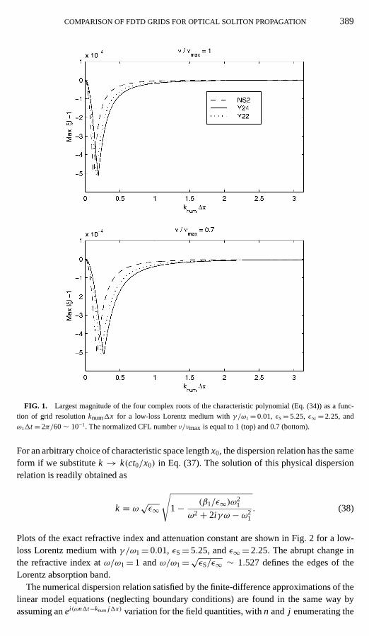
The amount of artificial dissipation introduced by the discrete ODEs is shown in Fig. 1as a function of the grid resolutionknum1x for a fixed normalized CFL numberν/νmax

equal to 1 and 0.7 (this last value lying slightly below the maximum CFL number 1/√

2for the Y22 scheme in 2D [1]). We consider the parameter valuesεS= 5.25,ε∞= 2.25 asin [3] and a medium resonance-frequency resolutionω11t = 2π/60∼ 10−1. The case of alow-loss Lorentz medium withγ /ω1= 0.01 is shown. The discretization-induced numericaldissipation is very small for all schemes, with a peak value of∼5×10−4. We note that NS2has a slightly narrower peak in both graphs.

Assuming a space-time harmonic variationei (ωt−kx) of all fields, the exact (physical)dispersion relation associated with the linear part of Eq. (20) is readily obtained in dimen-sionless form as

ε∞ω4+ 2i ε∞γω3− [k2+ εSω21

]ω2− 2i γ k2ω + k2ω2

1 = 0. (37)


FIG. 1. Largest magnitude of the four complex roots of the characteristic polynomial (Eq. (34)) as a func-tion of grid resolutionknum1x for a low-loss Lorentz medium withγ /ω1= 0.01, εS= 5.25, ε∞ = 2.25, andω11t = 2π/60∼ 10−1. The normalized CFL numberν/νmax is equal to 1 (top) and 0.7 (bottom).

For an arbitrary choice of characteristic space lengthx0, the dispersion relation has the sameform if we substitutek → k(ct0/x0) in Eq. (37). The solution of this physical dispersionrelation is readily obtained as

k = ω√ε∞√

1− (β1/ε∞)ω21

ω2+ 2i γω − ω21

. (38)

Plots of the exact refractive index and attenuation constant are shown in Fig. 2 for a low-loss Lorentz medium withγ /ω1= 0.01, εS= 5.25, andε∞= 2.25. The abrupt change inthe refractive index atω/ω1= 1 andω/ω1=

√εS/ε∞ ∼ 1.527 defines the edges of the

Lorentz absorption band.The numerical dispersion relation satisfied by the finite-difference approximations of the

linear model equations (neglecting boundary conditions) are found in the same way byassuming anei (ωn1t−knum j1x) variation for the field quantities, withn and j enumerating the


FIG. 2. Exact linear refractive index and attenuation coefficient of a Lorentz medium characterized byγ /ω1= 0.01,εS= 5.25, andε∞ = 2.25.

time step and spatial grid point, respectively, yielding

ε∞ω4+ i ε∞γ ω3−[(

η

41t2

)+ εS

ω21

4

]ω2− i γ ω

(η

41t2

)+(

η

41t2

)ω2

1

4= 0, (39)

whereη is given by Eq. (35), ¯ω= sin(ω1t/2)/1t , and the numerical medium relaxationand resonance frequencies are given by

γ = γ cos(ω1t/2), (40)

ω1 = ω1 cos(ω1t/2). (41)

The numerical dispersion relation (39) can be rewritten in the form

√η

21t= ω√ε∞

√1− (β1/ε∞)ω2

1/4

ω2+ i γ ω − ω21/4

, (42)

where√ηY24 andηNS2are cubic complex polynomials inknum1x whose analytical solutions

are known [16].The numerical solution may then be compared with the exact physical one given by

Eq. (38) as a function of the frequency resolutionω1t for fixed normalized CFL numberν/νmax≤ 1, γ /ω1 andω11t . Figure 3 shows plots of the following quantities: normalizedratio between the numerical and the exact phase velocity (also given by the normalized ratiobetween the exact and the numerical refractive index); normalized attenuation constant; nor-malized energy velocity; and normalized group velocity. Parameter values areγ /ω1= 0.01,ω11t = 2π/60,εS= 5.25, andε∞= 2.25. The normalized CFL number is set 30% below its


FIG. 3. Normalized phase velocity, attenuation constant, energy velocity, and group velocity across thepassband and absorption band of the Lorentz medium (γ /ω1= 0.01,ω11t = 2π/60, εS= 5.25, ε∞ = 2.25). Thenormalized CFL number is equal toν/νmax= 0.7.

maximum stability limit, i.e.,ν/νmax= 0.7. In Fig. 3, the data for each normalized quantityhave been graphed across four windows to provide the necessary graphical dynamic rangein each frequency regime. The windows illustrate frequency regimes below resonance, nearresonance, at the upper edge of the medium absorption band, and far above resonance wherethe frequencies are coarsely resolved. Figure 3 illustrates the following salient features:(1) All schemes have their highest normalized phase/dissipation errors at the coarsely re-solved high frequency (approximately given byωc/ω1 ∼ 2/(ω11t) sin−1(ν/νmax) ∼ 14.8)beyond which the fields decay exponentially and have an increasing phase velocity [25].


(2) All schemes have the same error level at the upper edge of the medium absorptionband (atω/ω1=

√εS/ε∞ ∼ 1.527). (3) In comparison to the Y22 scheme, the Y24 and

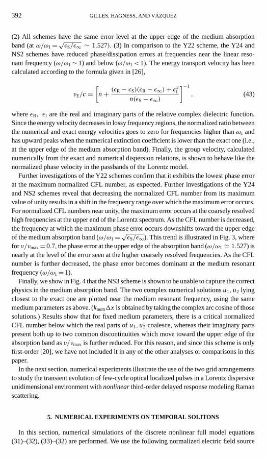
NS2 schemes have reduced phase/dissipation errors at frequencies near the linear reso-nant frequency (ω/ω1∼ 1) and below (ω/ω1< 1). The energy transport velocity has beencalculated according to the formula given in [26],

vE/c =[n+ (εR− εS)(εR− ε∞)+ ε2

I

n(εS− ε∞)]−1

, (43)

whereεR, εI are the real and imaginary parts of the relative complex dielectric function.Since the energy velocity decreases in lossy frequency regions, the normalized ratio betweenthe numerical and exact energy velocities goes to zero for frequencies higher thanωc andhas upward peaks when the numerical extinction coefficient is lower than the exact one (i.e.,at the upper edge of the medium absorption band). Finally, the group velocity, calculatednumerically from the exact and numerical dispersion relations, is shown to behave like thenormalized phase velocity in the passbands of the Lorentz model.

Further investigations of the Y22 schemes confirm that it exhibits the lowest phase errorat the maximum normalized CFL number, as expected. Further investigations of the Y24and NS2 schemes reveal that decreasing the normalized CFL number from its maximumvalue of unity results in a shift in the frequency range over which the maximum error occurs.For normalized CFL numbers near unity, the maximum error occurs at the coarsely resolvedhigh frequencies at the upper end of the Lorentz spectrum. As the CFL number is decreased,the frequency at which the maximum phase error occurs downshifts toward the upper edgeof the medium absorption band (ω/ω1=

√εS/ε∞). This trend is illustrated in Fig. 3, where

for ν/νmax= 0.7, the phase error at the upper edge of the absorption band (ω/ω1 ' 1.527) isnearly at the level of the error seen at the higher coarsely resolved frequencies. As the CFLnumber is further decreased, the phase error becomes dominant at the medium resonantfrequency (ω/ω1= 1).

Finally, we show in Fig. 4 that the NS3 scheme is shown to be unable to capture the correctphysics in the medium absorption band. The two complex numerical solutionsu1, u2 lyingclosest to the exact one are plotted near the medium resonant frequency, using the samemedium parameters as above. (knum1x is obtained by taking the complex arc cosine of thosesolutions.) Results show that for fixed medium parameters, there is a critical normalizedCFL number below which the real parts ofu1, u2 coalesce, whereas their imaginary partspresent both up to two common discontinuities which move toward the upper edge of theabsorption band asν/νmax is further reduced. For this reason, and since this scheme is onlyfirst-order [20], we have not included it in any of the other analyses or comparisons in thispaper.

In the next section, numerical experiments illustrate the use of the two grid arrangementsto study the transient evolution of few-cycle optical localized pulses in a Lorentz dispersiveunidimensional environment withnonlinearthird-order delayed response modeling Ramanscattering.

5. NUMERICAL EXPERIMENTS ON TEMPORAL SOLITONS

In this section, numerical simulations of the discrete nonlinear full model equations(31)–(32), (33)–(32) are performed. We use the following normalized electric field source


FIG. 4. The two complex numerical solutionsu1, u2 of the NS3 scheme lying closest to the exact one.Parameter values areγ /ω1= 0.01,ω11t = 2π/60,εS= 5.25, andε∞ = 2.25.

condition at the left grid boundary,

E(x = 0, t) = f (t) cos(ω0t), (44)

where f (t)= N sech(t/t0), t0 (related to the full width at half-peak intensity bytFWHM '1.76t0) is the characteristic time scale of the initial pulse envelope of normalized peakamplitudeN, and N defines the number of solitons forming the multisoliton pulse [24].The unstaggered grid arrangement requires the additional knowledge of the initialH values,which can be approximately obtained taking into account the linear group velocity (GV)and group velocity dispersion (GVD) of the pulse from the Fourier integral

H(x = 0, t) =∫ ∞−∞

H(ω)eiωt dω, (45)

where

H(ω) = 1

ZE(ω), (46)

and the linear impedance defined as the ratio of the electric over magnetic Fourier mag-nitudes is equal toZ=−ω/k. Performing a Taylor expansion ofk(ω) aroundω=ω0


yields

H(x = 0, t) ' 1

2

[1

Z0f (t)− i

(1

Z0

)′f ′(t)− 1

2

(1

Z0

)′′f ′′(t)

]eiω0t + c.c., (47)

where the impedance and its derivatives are all calculated atω=ω0.In order to obtain solitonlike behavior from the balance of dispersion (GVD) and Kerr

nonlinearity (SPM), the initial normalized peak amplitudeN and pulse widtht0 of thescaled electric field in Eq. (44) have to be properly adjusted according to the nonlinearSchrodinger (NLS) equation. When the electromagnetic fields are assumed to be circularlypolarized, a standard reductive perturbation method (RPM) [29] within the slowly vary-ing envelope approximation (SVEA) is used to reduce them to the NLS equation. Thisasymptotic reduction is carried out in a coordinate system moving with the pulse in space(spatial soliton) or in time (temporal soliton). Formally, this is done by introducing theslowly varying variablesξ = ε(x − ω′0t), τ = ε2t , or equivalently the dual slow variablesξ = ε2x, τ = ε(t−k′0x)which yields the one-dimensional NLS equation respectively in theform

iqτ + 1

2

ξ20

TDqξξ + 1

TNL|q|2q = 0, (48)

iqξ + 1

2

τ 20

LDqττ + 1

LNL|q|2q = 0. (49)

ε is the small perturbation parameterε ∼ O(1ω/ω0)¿ 1 (quasi-monochromatic approx-imation).

The characteristic dispersive and nonlinear length scales [21] are given by

TD = ξ20

ω′′0, TNL = 2k0c2

acircω20ω′0

= c

n2ω0ω′0, (50)

LD = −τ20

k′′0= (ω′0τ0/ξ0)

2ω′0TD, LNL = ω′0TNL, (51)

where we used the fact that for circular polarization, Eq. (29) is replaced byacirc ' 2n0n2,that is,a = (4/3)acirc. The balance between the dispersive and nonlinear length (time)scales, written respectively as

TNL = TD, LNL = LD, (52)

provides the appropriate value for the nonlinear parametera to obtain solitonlike behavior.Note that from the definition of the dual moving frames,ξ0=−ω′0τ0, this value is identical inboth moving coordinate systems. However, for the Maxwell’s equations we have chosen tonormalize space by the free-space velocityc, i.e.,ξ0= x0= ct0, and hence(ω′0t0/x0)

2 6= 1,meaning that the value ofa obtained for the driving boundary conditions (Eqs. (44) and(47)) that is used here will be different by a factor(ω′0/c)

2 from that obtained using initialconditions given by specifying all fields (including the polarization) att = 0 like is done in[17].


FIG. 5. (a) Linear refractive index and (b) the nonlinear Raman gain and nonlinear index (dashed curve)spectra. The pulse spectrum has been superimposed for comparison. Normalized linear Lorentz and Ramanparameters areγ /ω1= 10−6, ω1= 5.84,εS= 5.25,ε∞ = 2.25,θ = 0.3, γV/ÄV ' 0.356, andÄV = 1.28.

5.1. Decay of Higher-Order Temporal Solitons

The physical linear refractive index and the nonlinear Raman gain and nonlinear index(dashed curve) spectra are shown in Fig. 5.

The source spectrum has been superimposed for comparison. The long relaxation time(small dampingγ /ω1= 10−6) of the resonance causes two deep jumps of the linear refractiveindex atω ∼ ω1 andω ∼ ω1

√εS/ε∞, which outside this absorption band increases

slowly with frequency toward its infinite frequency value of√ε∞. The Lorentz medium

exhibits anomalous (normal) dispersionω′′ > 0 (ω′′< 0) over the spectral domain above(below) the absorption band. We have chosen the same pulse parameters as in [3], i.e., aninitial hyperbolic secant bright soliton pulse of duration equal to 25.7 fs (FWHM) (timeconstantt0= 14.6 fs,ct0= 4.38µm) centered atω0/2π = 137 THz (ω0t0= 12.57) (vacuumwavelengthλ0= 2.19µm). Approximately 3.5 modulation cycles are contained within theFWHM. The parameters defining the Raman Lorentz model are [30]ν−1

V = 12.2 fs, γ−1V =

32 fs(νV t0∼ 1.2, γV t0∼ 0.456) (ÄV t0= 1.28). The largest gain occurs at a frequency shiftedupward by aboutÄV t0 corresponding to 13.2 THz, which is of the order of the initial solitonspectral width(ÄV/ω0 ' 0.1).

Figures 6 and 7 display results of the simulations of transient fundamental (N= 1)and second-order (N= 2) temporal soliton evolution, propagating in the nonlinear Ramanenvironment.


FIG. 6. Transient fundamental (N= 1) temporal soliton propagation in the nonlinear Raman environment forthe same medium parameters as in Fig. 5.

The relative strength of the Kerr and Raman interactions is chosen equal toθ = 0.3. Asimple exact 1D one-way ABC was used. Alternative implementations of radiation boundaryconditions for high-order stencils using ghost nodes have been derived by Petropoulos [31]and others. In order to globally preserve the accuracy of the schemes, these were closednear the boundary using fifth- and fourth-order-accurate one-sided approximations as in[32, 33]. All codes were run at half their linear CFL stability limit on a Sun Ultra 10class workstation with run times below 30 min. in all cases tested using dynamic arrays tominimize storage. All schemes are explicit and need only to call a standard Newton solverfor the cubic equation inEn+1.

The pulse central frequency was chosen atω0/ω1∼ 2.15 above the absorption band(anomalous dispersion region). The approximate value ofa required by the Maxwell’ssolver to obtain solitonlike dynamics can be obtained from the NLS balance equation (52)for the circular polarization with the choice of distance unitξ0= x0= ct0. For the drivingboundary condition Eqs. (44) and (47) and taking into account the Raman contribution, thisyieldsacirc(1− θ)= 3.78× 10−2. For the linear polarization,a= (4/3)acirc, which givesfor θ = 0.3 the valuea= 7× 10−2 found by Goorjian and Taflove. Attention must also bepaid to ensure sufficient spatial resolution due to the generation of third harmonics.

Several grid sizes have been used to explore the numerical stability and accuracy ofthe nonlinear codes. A spatial resolution1x ∼ λ0/64 (λ0 being the carrier wavelengthinside the medium) is sufficient to mitigate the effects of numerical dispersion in the cases


FIG. 7. Transient second-order (N= 2) temporal soliton propagation in the nonlinear Raman environmentfor the same medium parameters as in Fig. 5.

treated. To characterize the solitonlike propagation regime, a useful parameter is givenby the product of the peak pulse intensity and the square of its FWHM. For fundamentalsolitons, this measure of the “pulse area” is constant. Numerical results present excellentagreement between the unstaggered and staggered nonlinear FDTD-ADE schemes. Thesmall (less than 1%) deviation in the soliton parameters (width and pulse area) obtainedwith the unstaggered grid scheme can be attributed to the approximate source conditionneeded for the magnetic field colocated with the electric field atx= 0. Figures 6a and7a display the pulseE field at t = 380 fs andt = 871 fs corresponding to a propagationdistance equal tox= 55µm andx= 126µm, respectively. Also shown in Figs. 6b and7b is the transient evolution of the pulse parameters. Figures 6c and 7c and 6d and 7ddepict the pulse fundamental and third-harmonic spectra. The asymptotic height of eachsoliton resulting from the splitting of the initial second-order soliton (Fig. 7) into its com-ponents is roughly 2λI/N= 3/2, 1/2, whereλI are the imaginary eigenvalues obtainedfrom the inverse scattering theory (IST) [24]. Phase velocity mismatch leads to the sep-aration of the transient third-harmonic precursor generated by the initial condition fromthe main pulse traveling at a different group velocity. As a result of the interference be-tween this transient precursor and the stationary third-harmonic pulse continuously gen-erated and traveling with the main pulse, the third-harmonic spectrum exhibits a symmet-ric modulation and a continuous redshift due to the Raman self-scattering of the mainpulse.


6. CONCLUDING REMARKS

We have developed 1D vector Maxwell’s equations solvers based on the staggered gridoriginally proposed by Yee and an unstaggered NS2 scheme proposed by Liu and shownby Driscoll and Fornberg to be third-order-accurate to study the propagation of temporalsolitons in a single-resonance Lorentz medium with third-order Raman-like nonlinearity.The stability and accuracy of the linear version of the various FDTD-ADE schemes havebeen analyzed. We have found that all schemes have a stability criterion that depends onlyon ε∞, and that the stability limit for the NS2 scheme is higher than that for the Y22 andY24 schemes. In comparison to the Y22 schemes, the numerical phase velocity errors forthe higher-order schemes are greatly reduced at frequencies below the Lorentz absorptionband and around the medium resonance frequency. The numerical dissipation levels do notvary much between schemes, and overall are very small.

We have tested the staggered and unstaggered FDTD-ADE schemes on a relativelycomplicated class of third-order nonlinear optical problems: the modeling of higher-ordersolitonlike and third-harmonic dynamics. Numerical results using the unstaggered gridscheme are in excellent agreement with the results obtained using the staggered gridschemes. Use of colocated electric field schemes such as the NS2 unstaggered schemeinvestigated here may prove to be essential for modeling nonlinear optical pulse propa-gation in higher dimensions. For this application, the advantage of using an unstaggeredgrid over an uncolocated staggered grid appears to outweigh any disadvantage of havingto use an approximate boundary condition for the unstaggered grid where the fields arecolocated.

ACKNOWLEDGMENTS

The authors thank Dr. P. G. Petropoulos and the referees for helpful suggestions. L. Gilles acknowledges theHonorary Fellow appointment at the University of Wisconsin. This work was sponsored in part by the MadridAutonome Community (CAM) (Spain) and the Comisi´on Interministerial de Ciencia y Technolog´ıa of Spain(PB95-0426).

REFERENCES

1. A. Taflove and S. C. Hagness,Computational Electrodynamics: The Finite-Difference Time-Domain Method,2nd ed. (Artech House, Norwood, 2000); K. S. Kunz and R. J. Luebbers,The Finite Difference Time DomainMethod for Electromagnetics(CRC Press, Boca Raton, 1993).

2. R. M. Joseph, S. C. Hagness, and A. Taflove, Direct time integration of Maxwell’s equations in linear dispersivemedia with absorption for scattering and propagation of femtosecond electromagnetic pulses,Opt. Lett.16,1412 (1991).

3. P. M. Goorjian, A. Taflove, R. M. Joseph, and S. C. Hagness, Computational modeling of femtosecond opticalsolitons from Maxwell’s equations,IEEE J. Quantum Electron.28, 2416 (1992).

4. R. W. Ziolkowski and J. B. Judkins, Full-wave vector Maxwell’s equation modeling of the self-focusing ofultrashort optical pulses in a nonlinear Kerr medium exhibiting a finite response time,J. Opt. Soc. Am. B10,186 (1993).

5. R. M. Joseph, P. M. Goorjian, and A. Taflove, Direct time integration of Maxwell’s equations in 2-D dielec-tric waveguides for propagation and scattering of femtosecond electromagnetic solitons,Opt. Lett.18, 491(1993).

6. R. M. Joseph and A. Taflove, Spatial soliton deflection mechanism indicated by FDTD Maxwell’s equationsmodeling,IEEE Photon. Technol. Lett.6, 1251 (1994).


7. R. W. Ziolkowski and J. B. Judkins, Applications of the nonlinear finite difference time domain (NL-FDTD)method to pulse propagation in nonlinear media: Self-focusing and linear/nonlinear interfaces,Radio Sci.28,901 (1993).

8. R. W. Ziolkowski and J. B. Judkins, Nonlinear finite-difference time-domain modeling of linear and nonlinearcorrugated waveguides,J. Opt. Soc. Am. B11, 1565 (1994).

9. S. A. Basinger and D. J. Brady, Finite-difference time-domain modeling of dispersive nonlinear Fabry–Perotcavities,J. Opt. Soc. Am. B11, 1504 (1994).

10. R. M. Joseph and A. Taflove, FDTD Maxwell’s equations models for nonlinear electrodynamics and optics,IEEE Trans. Antennas Propag.45, 364 (1997).

11. P. G. Petropoulos, Stability and phase error analysis of FD-TD in dispersive dielectrics,IEEE Trans. AntennasPropag.42, 62 (1994).

12. J. L. Young, A. Kittichartphayak, Y. M. Kwok, and D. Sullivan, On the dispersion errors related to(FD)2TDtype schemes,IEEE Trans. Microwave Theory Technol.43, 1902 (1995).

13. S. A. Cummer, An analysis of new and existing FDTD methods for isotropic cold plasma and a method forimproving their accuracy,IEEE Trans. Antennas Propag.45, 392 (1997).

14. K. S. Yee, Numerical solution of initial boundary value problems involving Maxwell’s equations in isotropicmedia,IEEE Trans. Antennas Propag.14, 302 (1966).

15. P. G. Petropoulos, Phase error control for FD-TD methods of second and fourth order accuracy,IEEE Trans.Antennas Propag.42, 859 (1994).

16. W. H. Press,Numerical Recipes in Fortran: The Art of Scientific Computing, 2nd ed. (Cambridge, Univ. Press,England, 1992).

17. C. V. Hile and W. L. Kath, Numerical solutions of Maxwell’s equations for nonlinear-optical pulse propagation,J. Opt. Soc. Am. B13, 1135 (1996).

18. B. Fidel, E. Heyman, R. Kastner, and R. W. Ziolkowski, Hybrid ray-FDTD moving window approach to pulsepropagation,J. Comput. Phys.138, 480 (1997).

19. Y. Liu, Fourier analysis of numerical algorithms for the Maxwell’s equations,J. Comput. Phys.124, 396(1996); R. Janaswamy and Y. Liu, An unstaggered colocated finite-difference scheme for solving time-domainMaxwell’s equations in curvilinear coordinates,IEEE Trans. Antennas Propag.45, 1584 (1997).

20. T. A. Driscoll and B. Fornberg, Note on nonsymmetric finite differences for Maxwell’s equations,J. Comput.Phys.161, 723 (2000).

21. G. P. Agrawal,Nonlinear Fiber Optics, 2nd ed. (Academic Press, San Diego, 1995).

22. J. R. Taylor,Optical Solitons, Theory and Experiment(Cambridge Univ. Press, England, 1992).

23. L. Gilles, H. Bachiri, and L. V´azquez, Evolution of higher-order bright solitons in a nonlinear medium withmemory,Phys. Rev. E57, 6079 (1998).

24. J. Satsuma and N. Yajima, Initial value problems of one-dimensional self-modulation of nonlinear wavesin dispersive media,Prog. Theor. Phys. (Jpn.)55(suppl.), 284 (1974); F. Abdullaev, S. Darmanyan, andP. Khabibullaev,Optical Solitons(Springer-Verlag, Berlin, 1993).

25. J. B. Schneider and C. L. Wagner, FDTD dispersion revisited: Faster-than-light propagation,IEEE MicrowaveGuided Wave Lett.9, 54 (1999).

26. K. E. Oughstun and S. Shen, Velocity of energy transport for a time-harmonic field in a multiple-resonanceLorentz medium,J. Opt. Soc. Am. B5, 2395 (1988).

27. P. N. Butcher and D. Cotter,The Elements of Nonlinear Optics(Cambridge Univ. Press, England,1990).

28. R. Richtmyer and K. Morton,Difference Methods for Initial-Value Problems(Wiley, New York, 1967).

29. T. Taniuti, Reductive perturbation method and far fields of wave equations,Prog. Theor. Phys. (Jpn.),55(suppl.), 1 (1974); Y. Kodama and A. Hasegawa, Nonlinear pulse propagation in a monomode dielec-tric guide,IEEE J. Quant. Electron.23, 510 (1987); T. Taniuti and K. Nishihara,Nonlinear Waves(Pitman,London, 1983).

30. K. J. Blow and D. Wood, Theoretical description of transient stimulated Raman scattering in optical fibers,IEEE J. Quant. Electron.25, 2665 (1989).


31. P. G. Petropoulos, L. Zhao, and A. Cangellaris, A reflectionless sponge layer absorbing boundary conditionfor the solution of Maxwell’s equations with high-order staggered finite difference schemes,J. Comput. Phys.139, 184 (1998).

32. A. Yefet and P. G. Petropoulos, A non-dissipative staggered fourth-order accurate explicit finite differencescheme for the time-domain Maxwell’s equations, submitted for publication.

33. M. H. Carpenter, D. Gottlieb, and S. Abarbanel, Stable and accurate boundary treatments for compact high-order finite-difference schemes,Appl. Numer. Anal.12, 55 (1993).

Comparison between Staggered and Unstaggered Finite ... · Comparison between Staggered and...

Documents

Transcript of Comparison between Staggered and Unstaggered Finite ... · Comparison between Staggered and...