Comparing Social Networks: Size, Density, and Local Structure
32
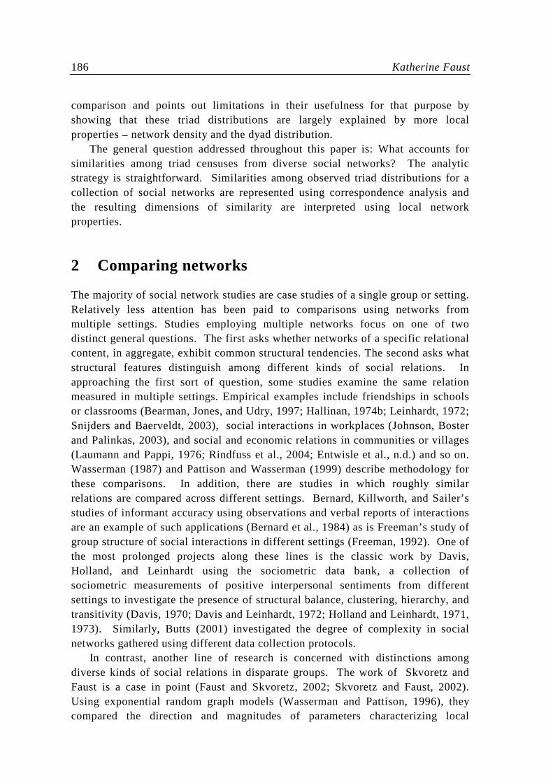
Metodološki zvezki, Vol. 3, No. 2, 2006, 185-216 Comparing Social Networks: Size, Density, and Local Structure Katherine Faust 1 Abstract This paper demonstrates limitations in usefulness of the triad census for studying similarities among local structural properties of social networks. A triad census succinctly summarizes the local structure of a network using the frequencies of sixteen isomorphism classes of triads (sub-graphs of three nodes). The empirical base for this study is a collection of 51 social networks measuring different relational contents (friendship, advice, agonistic encounters, victories in fights, dominance relations, and so on) among a variety of species (humans, chimpanzees, hyenas, monkeys, ponies, cows, and a number of bird species). Results show that, in aggregate, similarities among triad censuses of these empirical networks are largely explained by nodal and dyadic properties – the density of the network and distributions of mutual, asymmetric, and null dyads. These results remind us that the range of possible network-level properties is highly constrained by the size and density of the network and caution should be taken in interpreting higher order structural properties when they are largely explained by local network features. 1 Introduction This paper addresses several issues concerning local structure in social networks. Most generally, it continues the work of Skvoretz and Faust (Faust and Skvoretz, 2002; Skvoretz and Faust, 2002) modeling similarities in the structural features of diverse social networks. It also extends the idea of “structural signatures” for these comparisons (Skvoretz and Faust, 2002). In addition to these methodological contributions, the empirical example provides insights into the local nature of the structures of a diverse collection of social networks and in doing so challenges the basis for comparative modeling of higher order (macro) structures in networks. In particular, this paper uses triad censuses for network 1 Department of Sociology and Institute for Mathematical Behavioral Sciences; University of California, Irvine; Irvine, CA 92697 USA; [email protected]
Transcript of Comparing Social Networks: Size, Density, and Local Structure

Metodološki zvezki, Vol. 3, No. 2, 2006, 185-216
Comparing Social Networks: Size, Density, and Local Structure
Katherine Faust1
Abstract
This paper demonstrates limitations in usefulness of the triad census for studying similarities among local structural properties of social networks. A triad census succinctly summarizes the local structure of a network using the frequencies of sixteen isomorphism classes of triads (sub-graphs of three nodes). The empirical base for this study is a collection of 51 social networks measuring different relational contents (friendship, advice, agonistic encounters, victories in fights, dominance relations, and so on) among a variety of species (humans, chimpanzees, hyenas, monkeys, ponies, cows, and a number of bird species). Results show that, in aggregate, similarities among triad censuses of these empirical networks are largely explained by nodal and dyadic properties – the density of the network and distributions of mutual, asymmetric, and null dyads. These results remind us that the range of possible network-level properties is highly constrained by the size and density of the network and caution should be taken in interpreting higher order structural properties when they are largely explained by local network features.
1 Introduction
This paper addresses several issues concerning local structure in social networks. Most generally, it continues the work of Skvoretz and Faust (Faust and Skvoretz, 2002; Skvoretz and Faust, 2002) modeling similarities in the structural features of diverse social networks. It also extends the idea of “structural signatures” for these comparisons (Skvoretz and Faust, 2002). In addition to these methodological contributions, the empirical example provides insights into the local nature of the structures of a diverse collection of social networks and in doing so challenges the basis for comparative modeling of higher order (macro) structures in networks. In particular, this paper uses triad censuses for network
1 Department of Sociology and Institute for Mathematical Behavioral Sciences; University of
California, Irvine; Irvine, CA 92697 USA; [email protected]
186 Katherine Faust
comparison and points out limitations in their usefulness for that purpose by showing that these triad distributions are largely explained by more local properties – network density and the dyad distribution.
The general question addressed throughout this paper is: What accounts for similarities among triad censuses from diverse social networks? The analytic strategy is straightforward. Similarities among observed triad distributions for a collection of social networks are represented using correspondence analysis and the resulting dimensions of similarity are interpreted using local network properties.
2 Comparing networks
The majority of social network studies are case studies of a single group or setting. Relatively less attention has been paid to comparisons using networks from multiple settings. Studies employing multiple networks focus on one of two distinct general questions. The first asks whether networks of a specific relational content, in aggregate, exhibit common structural tendencies. The second asks what structural features distinguish among different kinds of social relations. In approaching the first sort of question, some studies examine the same relation measured in multiple settings. Empirical examples include friendships in schools or classrooms (Bearman, Jones, and Udry, 1997; Hallinan, 1974b; Leinhardt, 1972; Snijders and Baerveldt, 2003), social interactions in workplaces (Johnson, Boster and Palinkas, 2003), and social and economic relations in communities or villages (Laumann and Pappi, 1976; Rindfuss et al., 2004; Entwisle et al., n.d.) and so on. Wasserman (1987) and Pattison and Wasserman (1999) describe methodology for these comparisons. In addition, there are studies in which roughly similar relations are compared across different settings. Bernard, Killworth, and Sailer’s studies of informant accuracy using observations and verbal reports of interactions are an example of such applications (Bernard et al., 1984) as is Freeman’s study of group structure of social interactions in different settings (Freeman, 1992). One of the most prolonged projects along these lines is the classic work by Davis, Holland, and Leinhardt using the sociometric data bank, a collection of sociometric measurements of positive interpersonal sentiments from different settings to investigate the presence of structural balance, clustering, hierarchy, and transitivity (Davis, 1970; Davis and Leinhardt, 1972; Holland and Leinhardt, 1971, 1973). Similarly, Butts (2001) investigated the degree of complexity in social networks gathered using different data collection protocols.
In contrast, another line of research is concerned with distinctions among diverse kinds of social relations in disparate groups. The work of Skvoretz and Faust is a case in point (Faust and Skvoretz, 2002; Skvoretz and Faust, 2002). Using exponential random graph models (Wasserman and Pattison, 1996), they compared the direction and magnitudes of parameters characterizing local

Comparing Social Networks: Size, Density, and Local Structure 187
structure in graphs and calculated measures of dissimilarity between graphs for a variety of social networks. Results showed differences in the “structural signatures” of different kinds of relations, notably antagonistic relations such as fighting and dominance on the one hand, and relations of affection (friendship, liking) and affiliation on the other. Differences between species were apparent only for the first kind of relation, where humans showed tendencies toward mutuality and in-stars and away from transitivity whereas non-human primates showed tendencies in the opposite direction on these properties (Skvoretz and Faust, 2002).
The current work continues the line of inquiry initiated by Skvoretz and Faust. In particular, it uses the triad census as a vehicle for comparisons to investigate local structural similarities among a collection of 51 networks of different relational contents and measured on different species.
3 Notation
Social networks consist of social relationships between pairs or sets of social units, such as directed friendship choices between school children, victories in antagonistic encounters between fighting deer, or advice seeking between corporate managers. Formally, a social network for a directed dyadic relation consists of a set of social units, referred to as actors, and a set of linkages between pairs of actors, referred to as ties. Social networks are commonly represented by a graph or directed graph. In a directed graph nodes represent the social units in the network and arcs represent the directed ties between pairs of actors. A directed graph with node set V and arc set E is denoted G(V,E), with n the number of nodes in the graph. A social network or its associated directed graph can also be presented in a sociomatrix with n rows and columns indexing actors (in identical order). An entry in the sociomatrix codes the tie from the row actor to column actor. When a tie is either present or absent, the relation is dichotomous, taking on values of 0 or 1. In general self ties are undefined.
4 Local structure, isomorphism classes and subgraph censuses
There has been considerable and enduring interest in local structure in networks since the early years of social network studies. Local structure consists of configurations and properties of small subgraphs of nodes and arcs, most notably dyads and triads. A dyad is a subgraph of two nodes and the possible arcs between them. In a directed graph there are three isomorphism classes of dyads: mutual (M), asymmetric (A) ignoring the direction of the arc, and null (N). A triad is a
188 Katherine Faust
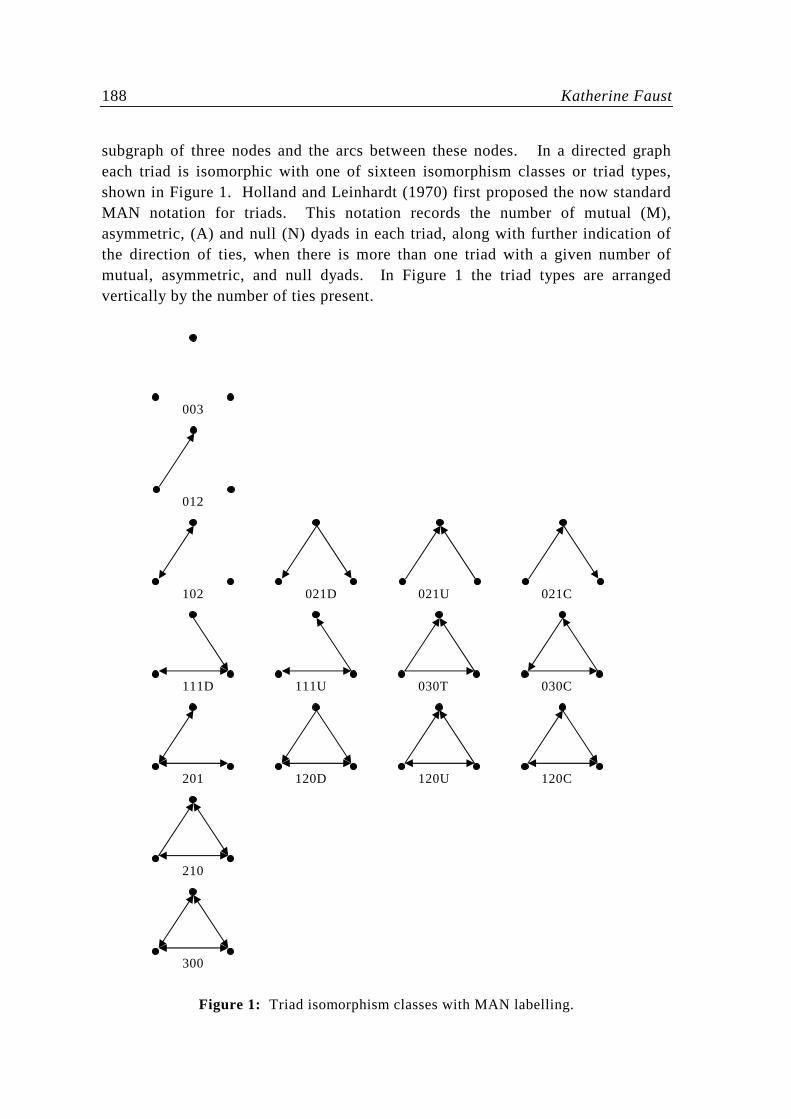
subgraph of three nodes and the arcs between these nodes. In a directed graph each triad is isomorphic with one of sixteen isomorphism classes or triad types, shown in Figure 1. Holland and Leinhardt (1970) first proposed the now standard MAN notation for triads. This notation records the number of mutual (M), asymmetric, (A) and null (N) dyads in each triad, along with further indication of the direction of ties, when there is more than one triad with a given number of mutual, asymmetric, and null dyads. In Figure 1 the triad types are arranged vertically by the number of ties present.
Figure 1: Triad isomorphism classes with MAN labelling.
003
021D 021U 021C
111D 111U 030T 030C
201
210
102
300
120D 120U 120C
012

Comparing Social Networks: Size, Density, and Local Structure 189
A standard vehicle for studying local structure is a subgraph census. A subgraph census records the frequency of each isomorphism class observed in a directed graph or network. For example, a dyad census records the number of mutual, asymmetric, and null dyads in a network. Similarly, a triad census records the number of triads in each of the sixteen triad isomorphism classes.
The appeal of the triad census as a means for investigating structural patterns in social networks lies in the fact that it succinctly summarizes a large amount of information about a network while retaining information about theoretically
important structures. In a directed graph of n nodes there are
3
ntriads. This
quantity increases rapidly as the size of the graph increases, making summary into sixteen isomorphism classes a substantial simplification (Wasserman and Faust, 1994). Nevertheless, this summary retains important information about local features of the network and allows one to test hypotheses about the prevalence of structural properties such as transitivity or intransitivity.
5 Macro structures and the triad census
Research employing triads and triad censuses has proved fruitful and long lived, largely due to the important theoretical properties embodied in triads and the links they afford between local (micro) structures and global (macro) structures (Davis, 1967, 1970; Davis and Leinhardt, 1972; Holland and Leinhardt, 1971; Johnsen, 1985, 1986, 1989, 1998; Friedkin, 1998). Whereas micro structures pertain to small subgraphs and properties measured on them, macro structures characterize the entire graph or network. Usefulness the triad census for testing theoretical macro structures arises because some theoretical macro structures are contradicted by specific configurations of triads. Support for the macro theory is evaluated by examining empirical networks for the occurrence of triads inconsistent with the theory. Theories that have been expressed in triadic terms include structural balance, clusterability, ranked clusters, and transitivity.
Structural balance is one of the most straightforward theories expressed in triadic terms. In early work in this area, Cartwright and Harary (1956) generalized Heider’s (1946) cognitive balance notion to structural balance. As a macro structure, a balanced signed graph has two subgroups where all ties within each subgroup have positive signs and all ties between the two subgroups have negative signs. Structural balance also can be examined using directed rather than signed graphs (Johnsen, 1985, 1986, 1998), where mutual ties take the place of positive ties and null ties take the place of negative ties. In a balanced directed graph all mutual ties are within subgroups and all null ties are between subgroups. In a balanced directed graph only two kinds of triads are permitted: {300 and 102}. Other triads violate the theory.

190 Katherine Faust
The idea of structural balance was extended to the notion of clusterability by Davis (1967) to allow more than two subgroups. In a clusterable signed graph all positive ties are within subgroups and negative ties are between subgroups. In a clusterable directed graph three triads are permitted: {300, 102, 003}. All other triads violate the theory. As a substantive example, clusterability would characterize a relation such as friendship if there were multiple cliques of mutual friendships in a population, but no friendships between cliques.
Further generalizations of these ideas include ranked clusters (Davis, 1970; Davis and Leinhardt, 1972) and transitivity (Holland and Leinhardt, 1971). Ranked clusters extend the clustering model to allow directed ties between clusters. The permitted triads for this model are {300, 102, 003, 120D, 120U, 030T, 021D 021U}. This macro model would represent a population with multiple friendship cliques ranked in prestige or popularity, in which friendships between cliques are directed from lower to higher status clique members. Transitivity holds for a triple of distinct nodes if, whenever the i � j tie and the j � k ties are present, then the i � k tie is present. The transitivity model includes one triad in addition to those for ranked clusters: {300, 102, 003, 120D, 120U, 030T, 021D 021U, 012}. The macro structure for transitivity provides for separate systems of ranked clusters within a population. As a substantive example, this macro model would characterize friendships in a population where different categories of people maintained separate systems of ranked cliques.
Since these structural theories imply different profiles of triads, we expect to observe dissimilar triad distributions for social networks of diverse kinds of social relations. For example, relations of dominance (Chase, 1974) generally exhibit hierarchical patterns and would be expected to contain triads consistent with transitivity. On the other hand, affectionate interpersonal relations, such as friendship, would be expected to form subgroups of mutual ties, consistent with balance or clusterability. Thus, triad distributions should be useful for studying similarities and dissimilarities in the local structural properties of diverse social networks. The following section describes methodology for these comparisons.
6 Data and analysis strategy
6.1 Data The empirical base for this investigation is a collection 51 of social networks representing a variety of types of relations and animal species. This collection includes relations of dominance, friendship, advice seeking, grooming, fights, social grazing, non-agonistic social acts, email communications, and confiding, to name a few. Relations are measured among many different species, including humans, baboons, colobus monkeys, cows, hyenas, ponies, red deer, sparrows,

Comparing Social Networks: Size, Density, and Local Structure 191
willow tits, and vervet monkeys. These networks are a sample of social networks of the sort generally seen in the social network and ethology literatures and were compiled from widely available sources (for example the standard data in UCINET, journal articles, and other published sources). The Appendix lists and describes the networks and their sources. All networks are coded to be dichotomous and the ties are directed. The heterogeneity of relations in this sample is an advantage for the current analysis since the goal is to examine similarities and dissimilarities among the networks, rather than structural tendencies in a single type of relation. The initial expectation is that networks with similar social relations should exhibit similar structural tendencies and thus have similar profiles of triad censuses. Data to investigate this expectation consist of the triad census (expressed as relative frequencies) for each network in the set of 51. This information is arrayed in a matrix with the 51 networks on the rows and 16 triad types on the columns. The entries are the relative frequencies of each triad type for each network.
6.2 Analysis strategy
The logic of the analysis is as follows. The first step represents similarities among the networks based on their triad censuses and among triad types based on their distributions across networks. Correspondence analysis is used to produce a low dimensional representation of the similarities among networks and among types of triads. The second step in the analysis seeks to interpret the spatial configurations of networks and triads using local structural properties of the networks Correspondence analysis (Blasius and Greenacre, 1998; Greenacre and Blasius, 1994; Weller & Romney, 1990) is a method for studying relationships in two-way arrays, and results in a low dimensional representation of similarities in the data. It is accomplished through decomposition of a matrix into its basic structure using singular value decomposition (Clausen 1998; Weller and Romney, 1990; Digby and Kempton, 1987). In practice, a “normalized” version of the matrix is decomposed: entries in the original matrix are divided by the square root of the product of the row and column marginal totals prior to singular value decomposition. Let A be a rectangular matrix of positive entries with g rows and
h columns (where g ≥ h). Two diagonal matrices 2
1−R and 2
1−C have entries equal
to reciprocals of the row and column totals of A:
(6.1)
=+
−
ia
1diag2
1
R

192 Katherine Faust
(6.2)
Correspondence analysis is a singular value decomposition of the normalized
matrix: YXΛACR ′=−−
2
1
2
1
where Λ is a diagonal matrix of singular values, }{ kλ ,
andX and Y are the left and right singular. Graphic displays presented below use principal coordinates, iku (for rows) and jkv (for columns) where:
(6.3)
(6.4)
On each dimension these scores have weighted means equal to 0.0 and
weighted variances equal to the squared singular values: (6.5)
(6.6)
Squared singular values express the amount of variation (chi square distance) that is explained by each dimension in the model. The total amount of variation in the data is referred to as inertia (Greenacre, 1984; Greenacre and Blasius, 1994;
Clausen, 1998) and is equal to the sum of the squared singular values: ∑=
W
kk
1
2λ .
Table 1: Descriptive Statistics for 51 Networks.
Size
Mean Nodal Degree Density
Proportion Mutual
Proportion Asymmetric
Proportion Null
Proportion Transitive
Mean 20.51 5.06 0.37 0.15 0.43 0.42 0.64 Std. Deviation 16.89 2.93 0.20 0.17 0.28 0.30 0.20 Minimum 4 0.55 0.02 0.00 0.01 0.00 0.21 Maximum 73 13.75 0.86 0.81 0.93 0.98 0.98 Percentiles 25 10 2.62 0.21 0.03 0.19 0.15 0.52 50 14 4.64 0.43 0.07 0.40 0.41 0.63 75 28 6.83 0.50 0.23 0.73 0.69 0.80
=+
−
ja
1diag2
1
C
+
++=i
ikkik a
axu λ
jjkkjk a
ayv
+
++= λ
∑∑= ++
+
= ++
+ ==h
i
jjk
g
i
iik a
au
a
au
11
0
∑∑= ++
+
= ++
+ ==h
ik
jjk
g
i
iik a
au
a
au
1
22
1
2 λ
Comparing Social Networks: Size, Density, and Local Structure 193
7 Results
7.1 Descriptive statistics and triad censuses Descriptive statistics for the networks are presented in Table 12. These results show considerable variability among the networks in their size, density, dyadic distributions, and tendencies toward transitivity. Networks range from 4 to 43 members, with densities ranging from 0.02 to 0.86.
The triad censuses for the 51 networks are presented in Table 2. Censuses were calculated using an adapted version of the SAS program described by Moody (1998). Glancing at these distributions shows some notable distinctions among the networks. First, 003 (all null) triads are prevalent in friendships between adolescent boys (cole1 and cole2), grazing preference between cows (cowg), social licking between cows (cowl), and dominance between nursery school boys (kids2), accounting for more than 50% of the triads in these distributions. Completely mutual triads, 300, are rare across the networks, but reach almost 50% in the network of grooming between chimpanzees (chimp3). The 030T transitive triad is prevalent in agonistic bouts between baboons (baboon3), threats between Highland ponies (ponies), fights between adult rhesus monkeys (rhesus1 and rhesus6), dominance between sparrows (sparrow), and aggressive encounters between juvenile vervet monkeys (vervet2a).
7.2 Correspondence analysis, network and triad spaces
Turning now to similarities among the 51 tirad distributions, scores for the first four dimensions of the correspondence analysis of the network-by-triad census array are presented in Table 3, for both networks and triad types. The first four dimensions account for 33.8%, 24.9%, 10.7% and 8.3% of the inertia, respectively (77.7% of the total inertia).
2 The density of a network is the proportion of possible ties that are present. The measure of
mutuality is the proportion of dyads that are mutual: M/(M+A+N). The proportion of dyads that are asymmetric and null are computed similarly. The measure of transitivity is the number of transitive triples divided by the number of triples that meet the condition for possibly being transitive. Specifically, it is the proportion of i, j, k triples where the i�j tie and the j� k ties are present in which the i� k tie is also present.

194 Katherine Faust
Table 2: Triad distributions for 51 Networks, expressed as percentages.
Tryad type Network 003 012 102 021D 021U 021C 111D 111U 030T 030C 201 120D 120U 120C 210 300 baboonf 12 35 02 10 09 07 05 01 14 01 00 03 00 01 01 00 baboonm1 00 00 00 00 00 00 00 00 15 00 00 00 50 00 15 20 baboonm2 00 05 00 10 10 00 00 10 40 00 00 00 20 00 05 00 baboonm3 02 18 02 02 00 08 01 02 51 00 00 03 10 00 01 00 banka 13 36 02 12 08 05 03 01 15 00 01 03 00 01 00 00 bankc 21 33 08 06 12 04 05 04 04 00 01 02 02 00 00 00 bankf 38 29 11 05 04 03 04 02 00 00 00 02 01 00 00 01 banks 07 13 01 19 01 04 00 13 09 00 02 01 14 03 10 03 cattle 12 31 02 13 07 10 02 02 17 00 00 02 01 01 00 00 chimp1 00 08 01 10 19 06 01 04 42 00 00 01 05 02 01 00 chimp2 00 00 00 04 00 00 02 08 06 00 02 12 19 08 27 11 chimp3 00 00 02 00 00 00 04 00 00 00 17 00 01 00 27 49 cole1 81 12 06 00 00 00 00 00 00 00 00 00 00 00 00 00 cole2 79 14 06 00 00 00 00 00 00 00 00 00 00 00 00 00 colobus1 00 00 00 25 00 00 00 25 00 00 00 00 25 00 25 00 colobus2 00 00 10 20 00 00 20 00 00 00 00 10 00 10 20 10 colobus3 02 08 19 00 00 02 10 13 00 00 21 02 02 02 08 08 cowg 93 02 04 00 00 00 00 00 00 00 00 00 00 00 00 00 cowl 87 12 01 00 00 00 00 00 00 00 00 00 00 00 00 00 eiesk1 49 23 15 01 02 01 02 03 00 00 01 00 01 00 01 00 eiesk2 39 23 17 02 03 01 05 04 01 00 02 01 01 00 01 01 eiesm 20 09 12 06 00 01 01 13 01 00 14 01 02 00 08 10 fifth 29 32 21 02 02 01 02 03 01 00 01 02 01 01 01 01 fourth 19 25 28 04 02 02 05 05 01 00 03 02 01 01 03 01 hyenaf 55 31 01 06 01 02 00 01 02 00 00 00 01 00 00 00 hyenam 28 34 02 15 04 05 00 04 07 00 00 00 01 00 00 00 kids1 06 11 13 05 01 04 08 14 03 00 06 03 04 03 12 07 kids2 60 28 04 02 02 02 01 01 01 00 00 00 00 00 00 00 macaca 09 13 21 03 02 02 09 09 00 00 10 02 02 01 10 07 nfponies 21 41 00 12 06 08 00 00 13 00 00 00 00 00 00 00 patasf 00 00 00 03 03 05 00 00 81 01 00 05 02 00 00 00 patasg 38 29 14 02 01 03 03 04 00 00 02 00 00 01 01 01 ponies 00 01 00 02 04 04 01 02 52 00 00 17 12 01 04 00 prison 82 12 05 00 00 00 00 00 00 00 00 00 00 00 00 00 reddeer 06 20 09 06 00 00 00 26 00 00 09 00 11 00 06 09 rhesus1 00 00 00 03 00 09 00 03 74 00 00 03 09 00 00 00 rhesus2 00 10 00 00 00 40 00 00 50 00 00 00 00 00 00 00 rhesus4 01 07 00 10 10 16 01 01 45 01 00 04 01 02 01 00 rhesus5 00 25 00 10 08 16 00 01 37 00 00 01 02 00 00 00 rhesus6 00 03 01 13 01 05 00 02 61 01 00 10 02 01 03 00 silver 00 00 03 06 01 01 02 06 19 01 00 21 09 03 17 12 sparrow 01 08 00 09 05 09 01 01 54 01 00 05 03 01 00 00 third 10 21 19 05 04 04 06 08 03 00 04 05 02 01 06 03 tits 00 00 02 09 00 04 00 05 21 00 00 14 16 04 20 05 vcbf 35 22 20 03 01 02 03 06 01 00 01 02 01 00 01 01 vcg 09 14 17 05 02 02 06 12 03 00 06 05 03 02 08 05 vcw 28 27 14 05 03 04 03 05 02 00 00 03 02 01 01 01 vervet1a 01 11 00 16 08 08 03 03 37 00 00 05 05 02 01 00 vervet1m 02 07 01 15 12 02 04 04 34 00 01 08 05 02 03 00 vervet2a 00 00 01 08 01 00 01 01 71 00 00 14 04 00 01 00

Comparing Social Networks: Size, Density, and Local Structure 195
Table 3: Correspondence analysis of triad censuses, scores for networks and triads.
Dimension Network 1 2 3 4 baboonf 0.078 -0.360 -0.448 0.190 baboonm1 -0.980 1.141 1.395 0.307 baboonm2 -0.803 -0.187 0.378 0.473 baboonm3 -0.656 -0.573 0.110 -0.131 banka 0.133 -0.371 -0.420 0.191 bankc 0.402 -0.166 -0.422 0.283 bankf 0.756 -0.107 -0.175 0.117 banks -0.341 0.388 0.126 0.597 cattle 0.024 -0.411 -0.361 0.172 chimp1 -0.667 -0.563 -0.171 0.105 chimp2 -0.767 1.182 0.542 0.346 chimp3 -0.548 2.390 0.080 -1.675 cole1 1.358 -0.206 0.620 -0.222 cole2 1.336 -0.209 0.582 -0.205 colobus1 -0.641 0.906 0.516 1.320 colobus2 -0.406 1.013 -0.392 0.223 colobus3 -0.014 1.214 -0.841 -0.388 cowg 1.478 -0.225 0.869 -0.314 cowl 1.414 -0.267 0.772 -0.252 eiesk1 0.955 -0.026 -0.018 0.002 eiesk2 0.784 0.077 -0.213 0.037 eiesm 0.208 0.904 -0.289 -0.298 fifth 0.700 0.072 -0.388 0.124 fourth 0.517 0.274 -0.605 0.147 hyenaf 0.971 -0.275 0.242 0.036 hyenam 0.456 -0.286 -0.174 0.273 kids1 -0.102 0.782 -0.397 0.142 kids2 1.092 -0.229 0.250 -0.041 macaca 0.117 0.848 -0.602 -0.084 nfponies 0.304 -0.462 -0.293 0.153 patasf -1.081 -0.965 0.181 -0.570 patasg 0.797 0.011 -0.206 0.078 ponies -0.985 -0.427 0.354 -0.099 prison 1.369 -0.222 0.651 -0.225 reddeer80 0.768 -0.347 0.019 0.023 rhesus1 -1.071 -0.829 0.302 -0.393 rhesus2 -0.750 -1.008 -0.344 -0.644 rhesus4 -0.729 -0.721 -0.217 -0.172 rhesus5 -0.463 -0.695 -0.349 -0.060 rhesus6 -0.938 -0.675 0.094 -0.243 silver -0.799 0.642 0.341 -0.015 sparrow -0.783 -0.710 -0.058 -0.206 third 0.154 0.370 -0.550 0.188 tits -0.837 0.493 0.480 0.299 vcbf 0.725 0.112 -0.235 0.091 vcg 0.045 0.632 -0.461 0.122 vcw 0.539 0.003 -0.266 0.187 vervet1a -0.634 -0.477 -0.136 0.138 vervet1m -0.622 -0.291 -0.100 0.200 vervet2a -1.059 -0.739 0.265 -0.343 vervet2m -0.802 -0.426 -0.041 0.015

196 Katherine Faust
Triad 1 2 3 4 003 1.209 -0.179 0.452 -0.139 012 0.489 -0.207 -0.394 0.183 102 0.542 0.450 -0.657 0.053 021D -0.360 -0.066 -0.166 0.520 021U -0.243 -0.485 -0.399 0.258 021C -0.426 -0.693 -0.437 -0.295 111D -0.011 0.597 -0.738 0.066 111U -0.189 0.606 -0.220 0.623 030T -0.933 -0.760 0.126 -0.302 030C -0.681 -0.460 -0.195 -0.263 201 -0.011 1.538 -0.843 -0.940 120D -0.737 0.017 0.093 0.033 120U -0.859 0.589 0.999 0.732 120C -0.501 0.708 -0.199 0.390 210 -0.603 1.311 0.295 0.181 300 -0.543 1.955 0.256 -1.142
Dimension 1
2.01.51.0.50.0-.5-1.0-1.5
Dim
ensi
on 2
3.0
2.5
2.0
1.5
1.0
.5
0.0
-.5
-1.0
-1.5
Quintiles of Density
5
4
3
2
1
vervet2mvervet2avervet1mvervet1a vcwvcg vcbftits thirdsparrowsilver
rhesus6 rhesus5rhesus4rhesus2rhesus1 reddeer80 prisonponies patasgpatasf nfponiesmacaca
kids2kids1
hyenam hyenaffourthfiftheiesm eiesk2eiesk1 cowlcowgcolobus3colobus2colobus1
cole2cole1
chimp3chimp2chimp1 cattlebanks bankfbankcbankababoonm3baboonm2
baboonm1baboonf
Figure 2a: Correspondence analysis of triad censuses, network space.

Comparing Social Networks: Size, Density, and Local Structure 197
Dimension 1
2.01.51.0.50.0-.5-1.0-1.5
Dim
ensi
on 2
3.0
2.5
2.0
1.5
1.0
.5
0.0
-.5
-1.0
-1.5
Number of Ties
6
5
4
3
2
1
0
300210120C120U120D201
030C030T111U111D
021C021U021D 102012 003
Figure 2b: Correspondence analysis of triad censuses, triad space.
Graphic display of the scores for the first two dimensions are in Figures 2a and 2b, for network and triad spaces respectively. In each figure, points that are close in space have similar profiles. In Figure 2a networks that are close to one another have similar profiles of proportions in their triad censuses, whereas those that are far apart have different triad census profiles. In this figure we see that triad censuses for the networks of fights between yearling rhesus monkeys (rhesus2) and fights between patas monkeys (patasf) are similar to each other and different from networks of grooming between chimpanzees (chimp3). Triad distributions in these three networks are different from the distributions for grazing preference between cows (cowg), social licking between cows (cowl) and friendships in a prison (prison). Figure 2b presents the similarity space for triads. In this figure triad types that occur in similar proportions across the collection of networks are close together. There is a clear diagonal pattern in the similarity space for triad types, related to the number of ties in the triad. Triads with more ties (300) are toward the upper left of the figure whereas triads with fewer ties (003) are toward the lower right. Symbols for points in Figure 2b code the number of ties in the triad (from 0 to 6) and in Figure 2a code the density of the network (in quintiles).
We can also take a joint view of the relationship between networks and triad types, though, for ease of visualization the two configurations are presented in separate plots in Figures 2a and 2b. Viewing the displays in Figures 2a and 2b together, we see in the upper left of the plots that grooming between chimpanzees (chimp3), agonistic encounters between chimpanzees (chimp2), non-agonistic

198 Katherine Faust
social acts between colobus monkeys (colobus3), and dominance between male baboons (baboonm1) are associated with 300 triads. In the lower left of the figures, fights between yearling rhesus monkeys (rhesus2) and fights between female patas monkeys (patasf) are associated with the 030T, 030C, and 021C triads. In the lower right, cows grazing and cows licking (cowg and cowl), friendships between adolescents (cole1 and cole2) and friendships in a prison (prison) are associated with the 003 triad.
7.3 Interpreting the correspondence analysis dimensions
What are the bases for resemblance among these triad censuses? To investigate this question, let us look more closely at the dimensions of the correspondence analysis solution, focusing first on the network space. Specifically, the following correlations and scatterplots explore whether similarities among triad distributions for these networks are largely patterned by nodal and dyadic properties.
Density
1.0.8.6.4.20.0
Dim
ensi
on 1
2.0
1.5
1.0
.5
0.0
-.5
-1.0
-1.5
Figure 3: Scatterplot of correspondence analysis network space dimension 1 and the network density, N = 51 networks.

Comparing Social Networks: Size, Density, and Local Structure 199
Proportion Null Dyads
1.0.8.6.4.20.0-.2
Dim
ensi
on 1
2.0
1.5
1.0
.5
0.0
-.5
-1.0
-1.5
Figure 4: Scatterplot of correspondence analysis network space dimension 1 and the
proportion of null dyads, N = 51 networks.
Proportion Mutual Dyads
1.0.8.6.4.20.0-.2
Dim
ensi
on 2
2.5
2.0
1.5
1.0
.5
0.0
-.5
-1.0
-1.5
Figure 5: Scatterplot of correspondence analysis network space dimension 2 and the proportion of mutual dyads, N = 51 networks.
200 Katherine Faust
Proportion Null Dyads
1.0.8.6.4.20.0-.2
Dim
ensi
on 3
1.5
1.0
.5
0.0
-.5
-1.0
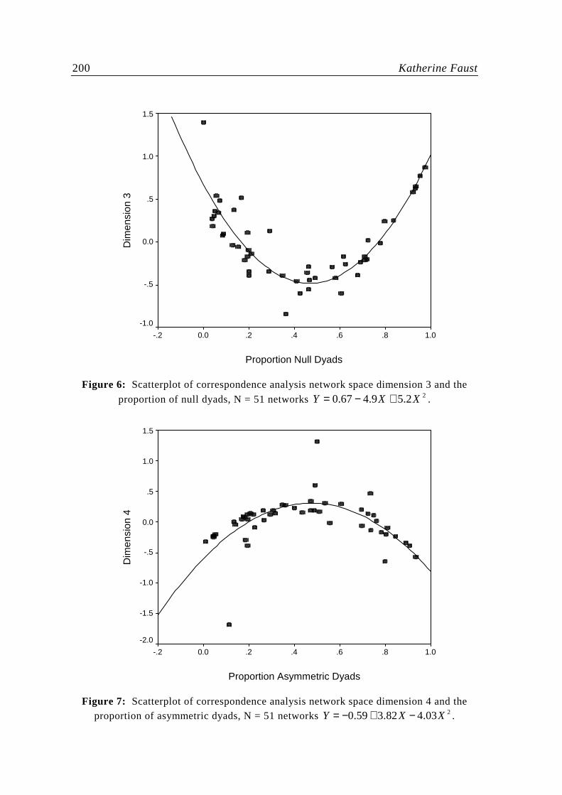
Figure 6: Scatterplot of correspondence analysis network space dimension 3 and the
proportion of null dyads, N = 51 networks 22.59.467.0 XXY +−= .
Proportion Asymmetric Dyads
1.0.8.6.4.20.0-.2
Dim
ensi
on 4
1.5
1.0
.5
0.0
-.5
-1.0
-1.5
-2.0
Figure 7: Scatterplot of correspondence analysis network space dimension 4 and the
proportion of asymmetric dyads, N = 51 networks 203.482.359.0 XXY −+−= .

Comparing Social Networks: Size, Density, and Local Structure 201
As suggested by the patterning of triad space, the first dimension of the correspondence analysis network space is associated with the density of the network – the correlation between coordinates on the first dimension and network density is r = -0.882. However, the correlation is even stronger with the proportion of dyads that are null; r = 0.994. The second dimension is associated with the level of mutuality in the network. This dimension correlates 0.941 with the proportion of dyads that are mutual. The third dimension is quadratic function relating to the proportion of dyads that are null; the best fitting quadratic equation relating scores on dimension three to the proportion of null dyads is
23.59.467.0 XXY +−= with =2r 0.792. The fourth dimension is related in a quadratic form to the asymmetry in the network, albeit weakly
( 203.482.359.0 XXY −+−= , =2r 0.410). Scatterplots of these relationships are shown in Figures 3 through 7.
Turning to the correspondence analysis space for triads, the first dimension correlates 0.962 with the proportion of null dyads in the triad; the second dimension correlates 0.956 with the proportion of mutual dyads; the third dimension is related in a quadratic function to the proportion of null dyads
( 225.321.067.0 XXY −+= , =2r 0.592); and the fourth dimension is a quadratic
function of the proportion of asymmetric dyads ( 206.328.353.0 XXY −+−= , =2r 0.519).
These results demonstrate that similarities among the triad distributions for these social networks are largely explained by very local properties, the nodal and dyadic distributions at most. In other words, modeling resemblance among these triad distributions does not require triadic level properties.
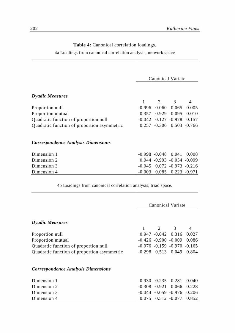
Canonical correlation analysis (Tatsuoka, 1971) provides a way to summarize the overall degree of linear relationship between the dimensions of the correspondence analysis and dyadic properties of the networks. The canonical correlation between two sets of variables is the maximum correlation between linear combinations of the variables in each set. For this analysis the first set consists of the four dyadic measures (the proportion null dyads, the proportion mutual dyads, the best fitting quadratic function of the proportion of asymmetric dyads, and the best fitting quadratic function of the proportion of null dyads) and the second set consists of the scores from the first four dimensions of correspondence analysis. Canonical correlation analysis is repeated separately for the network and the triad spaces.
202 Katherine Faust
Table 4: Canonical correlation loadings.
4a Loadings from canonical correlation analysis, network space
Canonical Variate
Dyadic Measures 1 2 3 4
Proportion null -0.996 0.060 0.065 0.005 Proportion mutual 0.357 -0.929 -0.095 0.010 Quadratic function of proportion null -0.042 0.127 -0.978 0.157 Quadratic function of proportion asymmetric 0.257 -0.306 0.503 -0.766
Correspondence Analysis Dimensions
Dimension 1 -0.998 -0.048 0.041 0.008 Dimension 2 0.044 -0.993 -0.054 -0.099 Dimension 3 -0.045 0.072 -0.973 -0.216 Dimension 4 -0.003 0.085 0.223 -0.971
4b Loadings from canonical correlation analysis, triad space.
Canonical Variate
Dyadic Measures 1 2 3 4
Proportion null 0.947 -0.042 0.316 0.027 Proportion mutual -0.426 -0.900 -0.009 0.086 Quadratic function of proportion null -0.076 -0.159 -0.970 -0.165 Quadratic function of proportion asymmetric -0.298 0.513 0.049 0.804
Correspondence Analysis Dimensions
Dimension 1 0.930 -0.235 0.281 0.040 Dimension 2 -0.308 -0.921 0.066 0.228 Dimension 3 -0.044 -0.059 -0.976 0.206 Dimension 4 0.075 0.512 -0.077 0.852

Comparing Social Networks: Size, Density, and Local Structure 203
For the network space, there are four significant canonical correlations (all with p < .0001), equal to 1.0, 0.999, 0.951, and 0.754, respectively. Together the first four canonical variates account for 86.7% of the variance in the first four dimensions of the correspondence analysis of the network space and 90.4% of the variance in the four dyadic network measures. Canonical loadings for the variables in the two sets are reported in Table 4a (The canonical loading is the correlation of the variable with the linear combination.). For the triad space there are also four significant canonical correlations (the first two with p < .0001, and the second two with p < .001), having values of 0.997, 0.979, 0.825, and 0.714 respectively.
In light of the fact that the first four dimensions of the correspondence analysis network space explain 77.7% of the inertia in the triad census distributions for these 51 networks, and dyadic level network properties account for 86.7% of this space, one might argue that around 67% (0.867 x 0.777) of the similarity among these triad distributions is accounted for by dyadic level network properties. Similarly, around 62% (0.802 x 0.777) of the similarity among triad types is accounted for by dyadic features of these triads.
In summary, these results demonstrate that, in aggregate, similarities in the triad censuses for a wide range of different social networks can largely be accounted for by dyadic level features of the networks. A reasonable estimate is that around two thirds of the variance among the networks’ triad distributions is accounted for by no more than nodal and dyadic features. How are we to interpret these results, and what are their implications for our understanding of social network structure? The following section addresses these questions.
8 Discussion and implications
Two related questions are raised by these results. First, what gives rise to the finding that similarity among triadic distributions is largely accounted for by lower order (nodal or dyadic) properties? Second, what are the implications of these result for comparisons of triad distributions in social networks? Clues to the answer these questions are found throughout the literature on triads and are provided more directly in literature on effects of network size and density on graph level indices. Four points are pertinent: effects of size and density on graph level measures; comparative use of triad censuses; absence of social structure in many social networks; and distinction between triad distributions and configurations of local structural properties.

204 Katherine Faust
8.1 Size and density
Network size has been recognized an issue in studies of triads since their earliest empirical use. In his 1970 paper on clustering and hierarchy, Davis (1970) analyzed 742 sociomatrices and presented results of triad distributions and statistics for triadic cycles separately for networks in five ranges of sizes. However, he does not reveal his rationale for doing so. Davis does note that for the 210 triad, which is not permitted under the ranked clusters model, “results are catastrophic in the larger groups” (1970: 845-846). Davis attributes the surplus of 210 triads in large networks to the frequency of fixed choice data collection designs that force otherwise mutual ties to be asymmetric. Johnsen (1985, 1986, 1998) pays considerably more attention to network size and its impact on possible micro and macro structural models. Picking up on Davis’ (1970) results for networks of different sizes, Johnsen (1985) observes that for network sizes 8 to 13, data perfectly fit the ranked clusters of mutual cliques model. Friedkin (1998: 143) addresses the point more extensively in his discussion of macro models for large networks. With respect to the 003 triad (all null dyads) he notes that “… especially in large groups, the possibility of three N linked actors should not be forbidden” (Friedkin, 1998: 143, emphasis in the original).3 So, authors have recognized the relationship between network size and triadic macro models, but have not addressed the issue directly.
Importantly, network density and not network size, per se, is crucial for understanding the distribution of triadic configurations. The density, d, of a network is the number of arcs in the network divided by the possible number of arcs. If the average number of arcs from each node is fixed, the total number of arcs increases as a linear function of network size but the possible number of arcs increases with the square of network size. Thus, if the average number of arcs from each node is fixed, a reasonable assumption if actors can only maintain a limited number of ties, then network density must decrease with network size. Why is this important?
Given the density of the network, the range of possible triad distributions is heavily constrained. Some triad types have extremely low probabilities, simply because of the density of the network. Formulae for the probability of each of the 16 triad types, given network density, are presented in Skvoretz et al. (2004). To
illustrate, the probability of a 300 triad (all mutual ties) is equal to 6d . In a network with 10 actors and 3 ties per actor, the density is equal to .33, and the probability of a 300 triad is 0.0014. If the size of the network is increased to 100,
3 Network size is also mentioned in discussions of its effect on statistics for testing structural
hypotheses, but largely in the context of its effect on the standard errors. It is easier to detect departures from expected frequencies in larger groups than in smaller groups (Leinhardt 1972, Hallinan 1974a, Holland and Leinhardt 1975).

Comparing Social Networks: Size, Density, and Local Structure 205
but the mean number of ties per actor remains 3, the density decreases to 0.03, and the probability of a 300 triad is 0.0000000008.
Table 5: Triad census of the routing data.
Triad Count Percent
003 322,769,974,374,083 99.99252370409 012 23,955,959,979 0.00742143658 102 175,605,448 0.00005440169 021D 882,596 0.00000027342 021U 109,179 0.00000003382 021C 444,490 0.00000013770 111D 4917 0.00000000152 111U 15,508 0.00000000480 030T 17,107 0.00000000530 030C 111 0.00000000003 201 1002 0.00000000031 120D 899 0.00000000028 120U 1120 0.00000000035 120C 96 0.00000000003 210 121 0.00000000004 300 69 0.00000000002
Total 322,794,107,416,725 Adapted from Vladimir Batagelj and Andrej Mrvar (2001): A subquadratic triad census algorithm for large sparse networks with small maximum degree. Social Networks, 23, 237–243.
To put the effect of size and density in sharper perspective for comparing
empirical networks, consider the network of routing linkages on the internet analyzed by Batagelj and Mrvar (2001). This network has 124,651 nodes and 207,214 edges. The mean number of ties per node is 3.3 and the density is 0.000027. The triad census for the routing network, expressed as a percentage distribution, is in Table 5. There are 322,794,107,416,725 triads in this network, of which 322,769,974,374,083, or 99.99%, are completely null (type 003). This is slightly less than the percent expected, given the density of the network (99.99999999%). In this network 69 triads, 0.00000000002%, are entirely mutual (type 300), which is more than the expected percent of 8.6x10-63%. For comparative purposes, consider what happens when the routing triad census is included in a correspondence analysis with the set of 51 networks analyzed above. The extremely low density of this network severely constrains its possible locations in the space of similarities among networks. Figure 8 presents the first two dimensions of the correspondence analysis of 52 networks (the first four dimensions account for 34.1%, 24.4%, 11.3% and 8.2% of the inertia). As expected, Batagelj and Mrvar’s network is in the far lower right corner with the other low density networks. Given its density, it is virtually impossible for it to occupy any other region of the space.

206 Katherine Faust
Dimension 1
2.52.01.51.0.50.0-.5-1.0-1.5-2.0
Dim
ensi
on 2
3.0
2.5
2.0
1.5
1.0
.5
0.0
-.5
-1.0
-1.5
Batagelj & Mrvar
Figure 8: Correspondence analysis dimensions 1 and 2 for 52 triad censuses including Batagelj and Mrvar’s internet routing network, network space.
In contrast, consider the network of non-agonistic social encounters in a group of 5 colobus monkeys (labeled colobus2 in Figure 2). This network is toward the upper left corner of both correspondence analysis figures for the first two dimensions (Figures 2 and 8). In the colobus monkey network the mean number of ties per monkey is 2.4, less than the mean for the routing network, and its density is 0.6. Of its 10 triads, none is completely null (003), though based on the density of the network 0.4% are expected to be so. This network has one triad that is completely mutual (type 300); 10% compared to an expectation of 4.7%. Given the network’s density it is almost impossible for it to occupy the lower right corner of the correspondence analysis space and be associated with the 003 triad.
Clearly these two illustrative networks are extreme in terms of size and density. However, regardless of other features they might share, because of their vastly different densities their triad distributions can not be similar.
The profound effect of density on graph level indices (GLIs) more generally is clearly demonstrated in Anderson Butts and Carley’s (1999) analyses. They conclude: “As we have seen, both size and density have powerful – and complex – interactions with other GLIs. These interactions stem from fundamental constraints on the space of graphs, constraints that severely limit the combinations of GLI values which can be realized on a given graph” (1999: 257). This is undoubtedly demonstrated in the triad census results presented here.

Comparing Social Networks: Size, Density, and Local Structure 207
8.2 Comparing triad distributions
The fact that, in aggregate, similarities among observed triad censuses are largely patterned by nodal and dyadic properties does not preclude higher order (i.e. triadic) structure in individual networks. In fact, 80% of the networks in the collection of 51, exhibit tendencies toward transitivity more than three standard deviations greater than expected, given their dyadic distributions. (Methodology for these tests is described in Holland and Leinhardt, 1976). Rather, the result suggests that the space of possible triad distributions is so constrained by network density and dyadic properties that comparing these distributions among networks that differ in these tendencies is uninformative. Little higher-order variability among the triad censuses remains to be explained.
8.3 Is there social structure in social networks?
As a third point addressing the questions posed above, it is important not to lose sight of the possibility that many social networks have little or no social structure. Holland and Leinhardt (1979) define social structure in network terms as the presence of higher order properties that are not adequately explained by nodal or dyadic tendencies. In other words, triads are the lowest level at which there is interesting social structure. With respect to the detection of triadic tendencies in the bank of 384 sociomatrices, Holland and Leinhardt (1979) found that when observed triad distributions were compared to those expected under different conditional distributions, a higher level of conditional distribution allowed fewer sociomatrices to exhibit significant tendencies away from intransitivity. They concluded that “… what was previously thought to be structure was spurious” (1979: 77) and that about 40% of the networks had no social structure.
Indeed, there may be many social networks in which there is little or no social structure in Holland and Leinhardt’s sense. This finding is reinforced more recently in Butts’s (2001) examination of the complexity of social networks. If networks exhibit patterns such as structural balance or classes of equivalent actors, then they should relatively “simple” compared to random graphs. They should not be algorithmically complex. However, evidence from networks collected by various methods (observations, self reports, and reports of others’ ties) fails to support this expectation, once network density is taken into account. The observation that graph structure is largely explained by local properties leads Butts to pose the conditional uniform graph distribution hypothesis: “…the aggregate distribution of empirically realized social networks is isomorphic with a uniform distribution over the space of all graphs, conditional on graph size and density” (Butts, 2001: 67). Moreover, if this hypothesis is correct “… much of what will be found—or not found—in any given graph will be driven heavily by density and graph size.” (Butts, 2001: 69).

208 Katherine Faust
Reiterating these observations, once we have taken lower order graph properties into account, there may be very little higher order structure in many social networks.
8.4 Configurations rather than triad distributions
As a final piece of the puzzle, reconsider the theoretically important structural information contained in triads. The discussion in section 5 above highlighted the linkage between macro structural theories and the particular triads that are consistent or inconsistent with them. These macro theories imply different triad census distributions A complementary approach to network structures links local properties and macro theories by focusing on configurations of relational ties between collections of actors rather than on the presence or absence of specific triads types. For example, transitivity is expressed for an ordered triple of distinct actors (i, j, k) such that if the i�j tie is present and the j� k tie is present, then the i� k tie is present. Transitivity is violated for an ordered triple of distinct actors (i, j, k) if the i�j tie is present and the j� k tie is present, but the i� k is absent. A network perfectly characterized by transitivity has transitive triple configurations but not intransitive triple configurations (other triple configurations are moot with respect to transitivity). The problem with using a triad census to examine transitivity is that individual triads types contain multiple configurations of ordered triples, some of which might be transitive and others intransitive. To illustrate, consider the 210 triad which is forbidden for the balance, clustering, ranked clusters, and transitivity macro models. This triad contains three ordered triples that are transitive and one that is intransitive, so on the whole it is shows a greater tendency toward rather than away from transitivity.
A slightly different implication of focusing on configurations of ties rather than triad censuses is presented in Davis’s (1979) review of the Davis, Holland, and Leinhardt work on triadic structure in networks. The persistent presence of the 210 triad led their research toward the study of transitivity and a focus on i,j,k triplets and other configurations rather than on triad distributions. As Davis notes, the focus on transitivity and sentiment patterns in triplets represented, for him, a retreat from a sociological perspective and “drifting back toward psychology” (Davis, 1979: 58) and “a slide from global structure to microanalysis” (1979: 60).
The results presented in this paper need not herald a turn away from sociology toward psychology. Rather, they remind us that system size and density, by mathematical necessity, constrain possible patterns of social organization (Mayhew and Levinger, 1976; Butts, 2001). Moreover, if lower-order properties (density and dyad distributions) account for a substantial portion of the systematic patterning of similarities among networks, parsimony and good scientific practice require that we not exert effort “explaining” the remainder.

Comparing Social Networks: Size, Density, and Local Structure 209
Acknowledgements
I would like to thank Vladimir Batagelj, Carter Butts, Lin Freeman, Kim Romney, John Skvoretz and participants in the UCI Social Network Research Group for comments on this research. I am grateful to Anuška Ferligoj, Andrej Blejec, and Janez Stare for the opportunity to present a version of this paper at the 2005 Applied Statistics Conference, Bled, Slovenia, September 2005.
References
[1] Anderson, B.S., Butts, C., and Carley, K. (1999): The interaction of size and density with graph-level indices. Social Networks, 21, 239-267.
[2] Batagelj, V. and Mrvar, A. (2001): A subquadratic triad census algorithm for large sparse networks with small maximum degree. Social Networks, 23, 237–243
[3] Bearman, P.S., Jones, J., and Udry, J.R. (1997): National Longitudinal Study of Adolescent Health: Research Design. Carolina Population Center. Unpublished manuscript.
[4] Bernard, H.R., Killworth, P., Kronenfeld, D., and Sailer, L. (1984): The problem of informant accuracy: The validity of retrospective data. Annual Review of Anthropology, 13, 495-517.
[5] Blasius, J. and Greenacre, M. (1998): Visualization of Categorical Data. New York: Academic Press.
[6] Butts, C.T. (2001): The complexity of social networks: theoretical and empirical findings. Social Networks, 23, 31-71.
[7] Cartwright, D. and Harary, F. (1956): Structural balance: A generalization of Heider’s theory. Psychological Review, 63, 277-293.
[8] Chase, I.D. (1974): Models of hierarchy formation in animal societies. Behavioral Science, 19, 374-382.
[9] Claussen, S. (1998): Applied Correspondence Analysis. Thousand Oaks: Sage.
[10] Davis, J.A. (1967): Clustering and structural balance in graphs. Human Relations, 20, 181-187.
[11] Davis, J.A. (1970): Clustering and hierarchy in interpersonal relations: Testing two graph theoretical models on 742 sociomatrices. American Sociological Review, 35, 843-851.
[12] Davis, J.A. (1979): The Davis/Holland/Leinhardt studies: An overview. In P.W. Holland and S. Leinhardt (Eds): Perspectives on Social Network Research, 51-62. New York: Academic Press.

210 Katherine Faust
[13] Davis, J.A. and Leinhardt, S. (1972): The structure of positive interpersonal relations in small groups. In J. Berger, M. Zeldith Jr. and B. Anderson (Eds): Sociological Theories in Progress, 2, 218-251. Boston: Houghton Mifflin.
[14] Digby, P.G.N. and Kempton, R.A. (1987): Multivariate Analysis of Ecological Communities. London: Chapman and Hall.
[15] Entwisle, B., Faust, K. Rindfuss, R., and Kaneda, T. (n.d.): Networks and contexts: Variation in the structure of social ties.
[16] Faust, K. and Skvoretz, J. (2002): Comparing networks across space and time, size and species. Sociological Methodology, 32, 267-299.
[17] Freeman, L.C. (1992): The sociological concept of `group': An empirical test of two models. American Journal of Sociology, 98, 152-166.
[18] Friedkin, N. (1998): A Structural Theory of Social Influence. New York: Cambridge University Press.
[19] Gifi, A. (1990): Nonlinear Multivariate Analysis. New York: John Wiley.
[20] Greenacre, M. (1984): Theory and Applications of Correspondence Analysis. New York: Academic Press.
[21] Greenacre, M. and Blasius, J. (Eds) (1994): Correspondence Analysis in the Social Sciences: Recent Developments and Applications. New York: Academic Press.
[22] Hallinan, M.T. (1974a): The Structure of Positive Sentiment. New York: Elsevier.
[23] Hallinan, M.T. (1974b): A structural model of sentiment relations. American Journal of Sociology, 80, 364-378.
[24] Heider, F. (1946): Attitudes and cognitive organization. Journal of Psychology, 21, 107-112.
[25] Holland, P.W. and Leinhardt, S. (1970): A method for detecting structure in sociometric data. American Journal of Sociology, 76, 492-513.
[26] Holland, P.W. and Leinhardt, S. (1971): Transitivity in structural models of small groups. Comparative Group Studies, 2, 107-124.
[27] Holland, P.W. and Leinhardt, S. (1972): Some evidence on the transitivity of positive interpersonal sentiment. American Journal of Sociology, 77, 1205-1209.
[28] Holland, P.W. and Leinhardt, S. (1976): Local structure in social networks. Sociological Methodology, 7, 1-45.
[29] Holland, P.W. and Leinhardt, S. (1979): Structural Sociometry. In P.W. Holland and S. Leinhardt (Eds): Perspectives on Social Network Research, 63-83. New York: Academic Press.
[30] Johnsen, E.C. (1985): Network macrostructure models for the Davis-Leinhardt set of empirical sociomatrices. Social Networks, 7, 203-224.

Comparing Social Networks: Size, Density, and Local Structure 211
[31] Johnsen, E.C. (1986): Structure and process: Agreement models for friendship formation. Social Networks, 8, 257-306.
[32] Johnsen, E.C. (1989): The micro-macro connection: Exact structure and process. In F. Roberts (Ed): Applications of Combinatorics and Graph Theory to the Biological and Social Sciences, 169-201. New York: Springer-Verlag.
[33] Johnsen, E.C. (1998): Structures and processes of solidarity: An initial formalization. In P. Doreian and T. Fararo (Eds): The Problem of Solidarity: Theories and Models, 263-302. Amsterdam: Gordon and Breach.
[34] Johnson, J.C., Boster, J.S., and Palinkas, L.A. (2003): Social roles and the evolution of networks in extreme and isolated environments. Journal of Mathematical Sociology, 27, 89-121,
[35] Laumann, E.O. and Pappi, P. (1976): Networks of Collective Action: A Perspective on Community Influence Systems. New York: Academic Press.
[36] Leinhardt, S. (1972): Developmental change in the sentiment structure of children’s groups. American Sociological Review, 37, 202-212.
[37] Mayhew, B.H. and Levinger, R.L. (1976): Size and density of interaction in human aggregates. American Journal of Sociology, 82, 86-110
[38] Moody, J. (1998): Matrix methods for calculating the triad census. Social Networks, 20, 291-299.
[39] Pattison, P. and Wasserman, S. (1999): Logit models and logistic regressions for social networks: II. Multivariate relations. British Journal of Mathematical and Statistical Psychology, 52, 169-193.
[40] Rindfuss, R.R., Jampaklay, A., Entwisle, B., Sawangdee, Y., Faust, K., and Prasartkul, P. (2004): The Collection and Analysis of Social Network Data in Nang Rong, Thailand. In M. Morris (Ed): Network Epidemiology: A Handbook For Survey Design and Data Collection, 175-200. Oxford: Oxford University Press.
[41] Skvoretz, J., Fararo, T.J., and Agneessens, F. (2004): Advances in biased net theory: Definitions, derivations, and estimations. Social Networks, 26, 113-139.
[42] Skvoretz, J. and Faust, K. (2002): Relations, species, and network structure. Journal of Social Structure, 3. http://zeeb.library.cmu.edu:7850/JoSS/skvoretz/index.html
[43] Snijders T.A.B. and Baerveldt, C. (2003): A Multilevel Network Study of the Effects of Delinquent Behavior on Friendship Evolution. Journal of Mathematical Sociology, 27, 123-151.
[44] Tatsuoka, M.M. (1971): Multivariate Analysis: Techniques for Educational and Psychological Research. New York: John Wiley and Sons.
[45] Wasserman, S.S. (1977): Random directed graph distributions and the triad census in social networks. Journal of Mathematical Sociology, 5, 61-86.

212 Katherine Faust
[46] Wasserman, S.S. and Faust, K. (1994): Social Network Analysis: Methods and Applications. New York: Cambridge University Press.
[47] Wasserman, S.S. and Pattison, P. (1996): Logit models and logistic regressions for social networks: I. An introduction to markov graphs and p*. Psychometrika, 61, 401-425.
[48] Weller, Susan C. and A. Kimball Romney (1990): Metric Scaling: Correspondence Analysis. Newbury Park, CA: Sage.
References for social network data
[1] Anderson, C.J., Wasserman, S., and Crouch, B. (1999): A p* primer: Logit models for social networks. Social Networks, 21, 37-66.
[2] Appleby, M. (1983): The probability of linearity in hierarchies. Animal Behaviour, 31, 600-608.
[3] Clutton-Brock, T.H., Greenwood, P.J., and Powell, R.P. (1976): Ranks and relationships in highland ponies and highland cows. Zeitschrift fur Tierpsychologie, 41, 202-216.
[4] Coleman, J. (1964): Introduction to Mathematical Sociology. New York: Free Press.
[5] Dunbar, R.I.M. and Dunbar, E.P. (1976): Contrasts in social structure among black-and-white colobus monkey groups. Animal Behaviour, 24, 84-92.
[6] Frank, L.G. (1986): Social organization of the spotted hyaena crocuta crocuta. II: Dominance and reproduction. Animal Behaviour, 34, 1510-1527.
[7] Freeman, L.C., Freeman, S.C., and Romney, A.K. (1992): The implications of social structure for dominance hierarchies in red deer. Animal Behaviour, 44, 239-245.
[8] Freeman, S.C. and Freeman, L.C. (1979): The Networkers Network: A Study of the Impact of a New Communications Medium on Sociometric Structure. Social Science Research Reports, 46. Irvine, CA: University of California.
[9] Hall, K.R.L. and DeVore, I. (1965): Baboon social behavior. In I. DeVore (Ed): Primate Social Behavior: Field Studies of Monkeys and Apes, 53-110. New York: Holt, Rinehart, and Winston.
[10] Hausfater, G. (1975): Dominance and Reproduction in Baboons (Papio cynocephalus), a Quantitative Analysis. New York: S. Karger.
[11] Horrocks, J. and Hunte, W. (1983): Maternal rank and offspring rank in vervet monkeys: An appraisal of the mechanisms of rank acquisition. Animal Behaviour, 31, 772-782.
[12] Kaplan, J.R. and Zucker, E. (1980): Social organization in a group of free-ranging patas monkeys. Folia Primatologica, 34, 196-213.

Comparing Social Networks: Size, Density, and Local Structure 213
[13] Kikkawa, J. (1980): Weight change in relation to social hierarchy in captive flocks of silvereyes, zosterops lateralis. Behaviour, 74, 92-100.
[14] Lahti, K., Koivula, K., and Orell, M. (1994): Is the social hierarchy always linear in tits. Journal of Avian Biology, 25, 347-348.
[15] MacRae, D. (1960): Direct factor analysis of sociometric data. Sociometry, 23, 360-371.
[16] McGrew, W.C. (1972): An Ethological Study of Children's Behavior. New York: Academic Press.
[17] Nishida, T. and Kasuhiko H. (1996): Coalition strategies among male chimpanzees of the Mahale Mountains, Tanzania. In W.C. McGrew, L.F. Marchant, and T. Nishida (Eds): Great Ape Societies, 114-134. New York: Cambridge University Press.
[18] Parker, J.G. and Asher, S. (1993): Friendship and friendship quality in middle childhood: Links with per group acceptance and feelings of loneliness and social dissatisfaction. Developmental Psychology, 29, 611-621.
[19] Pattison, P., Wasserman, S., Robins, G., and Kanfer, A.M. (2000): Statistical evaluation of algebraic constraints for social networks. Journal of Mathematical Psychology, 44, 536-568.
[20] Reinhardt, V. and Reinhardt, A. (1981): Cohesive relationships in a cattle herd (bos indicus). Behaviour, 76, 121-151.
[21] Roberts, J.M.Jr. (1994): Fit of some models to red deer dominance data. Journal of Quantitative Anthropology, 4, 249-258.
[22] Roberts, John M.Jr. and Browning, B.A. (1998): Proximity and threats in highland ponies. Social Networks, 20, 227-238.
[23] Robins, G., Pattison, P., and Wasserman, S. (1999): Logit models and logistic regressions for social networks: III. Valued relations. Psychometrika, 64, 371-394.
[24] Sade, D.S. (1967): Determinants of dominance in a group of free-ranging rhesus monkeys. In S.A. Altmann (Ed): Social Communication among Primates, 99-114. Chicago: University of Chicago Press.
[25] Sade, D.S. (1989): Sociometrics of macaca mulatta III: N-path centrality in grooming networks. Social Networks, 11, 273-292.
[26] Schein, M.W. and Fohrman, M.H. (1955): Social dominance relationships in a herd of dairy cattle. The British Journal of Animal Behavior, 3, 45-55.
[27] Strayer, F.F. and Janet Strayer (1976): An ethological analysis of social agonism and dominance relations among preschool children. Child Development, 47, 980-989.
[28] Tufto, J., Solberg, E.J., and Ringgsby, T. (1998): Statistical models of transitive and intransitive dominance structures. Animal Behaviour, 55, 1489-1498.

214 Katherine Faust
[29] Tyler, S.J. (1972): The behaviour and social organization of the new forest pony. Animal Behavior Monographs, Volume 5, Part 2.
[30] Vickers, M. and Chan, S. (1981): Representing Classroom Social Structure. Melbourne: Victoria Institute of Secondary Education.
[31] Wasserman, S.S. and Faust, K. (1994): Social Network Analysis: Methods and Applications. New York: Cambridge University Press.
[32] Watt, D.J. (1986): Relationship of plumage variability, size and sex to social dominance. Animal Behaviour, 34, 16-27.
Appendix: List of social networks
The following list gives the label for each network along with a reference for the source of the data.
• baboonf: dominance interactions between female and one adult male baboons (Figure 3-8, page 69, Hall and DeVore, 1965)
• baboonm1 and baboonm2: dominance between male baboons (Table 3-2, page 60, Hall and DeVore, 1965)
• baboonm3: outcomes of agonistic bouts between male baboons (Table XI, page 39, Hausfater, 1975)
• banka: advice in a bank office (Table 5, page 558, Pattison et al., 2000) • bankc: confiding in a bank office (Table 5, page 558, Pattison et al., 2000) • bankf: close friends in a bank office (Table 5, page 558, Pattison et al.,
2000) • banks: satisfying interaction in a bank office (Table 5, page 558, Pattison
et al., 2000) • cattle: contests between dairy cattle (Figure 1, page 49, Schein and
Fohrman, 1955) • chimp1, chimp2, and chimp3: Three relations between Chimpanzees. pant-
grunt calls (Table 9.3, page 119), initiation of dyadic agonistic confrontations (Table 9.4, page 119), and initiation of grooming (Table 9.14a, page 126). Data from Nishida and Hosaka (1996).
• cole1 and cole2: friendship at two time points between adolescent boys (Table 14.5 pages 450-451, Coleman, 1964)
• colobus1, colobus2, colobus3: non-agonistic social acts between colobus monkeys in a small group (Table I, page 86, Dunbar and Dunbar, 1976)
• cowl, cowg: Two relations between cows, bos indicus. social licking (Figure 7, page 130) and social grazing (Figure 4, page 126). Data from Reinhardt and Reinhardt (1981).
Comparing Social Networks: Size, Density, and Local Structure 215
• eiesk1: EIES data, rating of acquaintanceship between social science researchers at time 1. Recoded 3,4=1, <3=0. (Freeman and Freeman, 1979; Table B.8, page 745, Wasserman and Faust, 1994)
• eiesk2: EIES data, rating of acquaintanceship between social science researchers at time 2. Recoded 3,4=1, <3=0. (Freeman and Freeman, 1979; Table B.9, page 746, Wasserman and Faust, 1994)
• eiesm: EIES data frequency of message sending between social science researchers, Recoded “1” if any message was sent. (Freeman and Freeman, 1979; Table B.10, page 747,Wasserman and Faust, 1994)
• fifth: friendships between fifth graders (Table 3, page 44, Anderson et al., 1999, data from Parker and Asher, 1993)
• fourth: friendships between fourth graders (Table 3, page 44, Anderson et al., 1999, data from Parker and Asher, 1993)
• hyenaf, hyenam: Dominance, among females and among males Hyaena, crocuta crocuta. Dominance among adult females (Table I, page 1513) and dominance among males (Table V, page 1519). Data from Frank (1986).
• kids1: initiated agonism between children (Figure 2, page 986, Strayer and Strayer, 1976)
• kids2: dominance among boys in a nursery school (Figure 5.5, page 125, McGrew, 1972)
• macaca: Grooming between Macaca Mulatta. (Table 1, page 274). Data from Sade (1989).
• nfponies: threats between ponies (Table XIV, page 122, Tyler, 1972) • patasf and patasg: Two relations between Patas monkeys: fighting (Table
III, page 202) and grooming (Table V, page 205). Data from Kaplan and Zucker (1980).
• ponies: Threats between Highland ponies. (Table 2, page 3). Data from Roberts and Browning (1998), originally in Clutton-Brock, Greenwood, and Powell (1976).
• prison: closest friendships in a prison (Table 1, page 363, MacRae, 1960) • reddeer80: Winner and loser in encounters between Red deer stags, Cervus
elaphus L. (Figure 1a, page 601) Data from Appleby (1983). Data also in Freeman, Freeman, and Romney (1992) and Roberts (1994).
• rhesus1: fights between adult female rhesus monkeys (Table 1, page 105, Sade, 1967)
• rhesus2: fights between yearling rhesus monkeys (Table 2, page 107, Sade, 1967)
• rhesus4: fights between adult rhesus monkeys (Table 4, page 108, Sade, 1967)
• rhesus5: fights between adult rhesus monkeys (Table 7, page 110, Sade, 1967)

216 Katherine Faust
• rhesus6: fights between adult rhesus monkeys (Table 8, page 111, Sade, 1967)
• silver: Victories in encounters between Silvereyes, zosterops lateralis. (Table 1, page 94). Data from Kikkawa (1980).
• sparrow: Dominance between Sparrows, zonotrichia querula, including both attacks and avoidances (Figure 2, page 19). Data from Watt (1986).
• third: friendship between third graders (Table 1, page 42, Anderson et al., 1999, data from Parker and Asher, 1993)
• tits: dominance between Willow tits, parus montanus. (Table 1, page 1492). Data from Tufto, Solberg, and Ringgsby (1998). Data originally in Lahti, Koivula, and Orell (1994).
• vcbf: best friends between seventh graders (Table 3, page 385, Robins, Pattison, and Wasserman, 1999, from Vickers and Chan, 1981)
• vcg: get on with between seventh graders (Table 11, page 422, Wasserman and Pattison, 1996, from Vickers and Chan, 1981)
• vcw: work with between seventh graders (Table 12, page 423, Wasserman and Pattison, 1996, from Vickers and Chan, 1981)
• vervet1a and vervet2a: Vervet monkeys (Cercopithecus aethiops sabaeus), juveniles from two troops (1 and 2) dyadic aggressive / submissive interactions, both mothers absent (Table II, page 776), Data from Horrocks and Hunte (1983).
• vervet1m and vervet2m: Vervet monkeys (Cercopithecus aethiops sabaeus), juveniles from two troops (1 and 2) dyadic aggressive/ submissive interactions, both mothers present (Table I, page 775), Data from Horrocks and Hunte (1983).