Comparing Networks Across Space and Time, Size and Species

8COMPARING NETWORKS ACROSSSPACE AND TIME, SIZE ANDSPECIES

Katherine Faust*John Skvoretz†

We describe and illustrate methodology for comparing networksfrom diverse settings. Our empirical base consists of 42 networksfrom four kinds of species (humans, nonhuman primates, nonpri-mate mammals, and birds) and covering distinct types of relationssuch as influence, grooming, and agonistic encounters. The gen-eral problem is to determine whether networks are similarly struc-tured despite their surface differences. The methodology we proposeis generally applicable to the characterization and comparison ofnetwork-level social structures across multiple settings, such as dif-ferent organizations, communities, or social groups, and to theexamination of sources of variability in network structure. We firstfit a p* model (Wasserman and Pattison 1996) to each network toobtain estimates for effects of six structural properties on the prob-ability of the graph. We then calculate predicted tie probabilities foreach network, using both its own parameter estimates and the esti-mates from every other network in the collection. Comparison isbased on the similarity between sets of predicted tie probabilities.We then use correspondence analysis to represent the similaritiesamong all 42 networks and interpret the resulting configurationusing information about the species and relations involved. Results

*University of California, Irvine†University of South CarolinaWe acknowledge the helpful comments of the editor and anonymous review-

ers. For their encouragement and suggestions on the research, we thank H. RussellBernard, Linton Freeman, and A. Kimball Romney. We thank Tracy Burkett and Doug-las Nigh for making their data available to us.

267

show that similarities among the networks are due more to the kindof relation than to the kind of animal.

1. INTRODUCTION

Much of social network analysis examines a single network at a time.Commonly the analyses comprise case studies of network properties orprocesses within a single community. For example, dominance relationsamong chimpanzees are described and the structure of the network ana-lyzed. Or the liking and disliking relations among novices in a monasteryare described and the patterning in these networks related to observationsabout group structure and dynamics. The problem of comparing networksarises more rarely, and when it does the usual context is that of comparingtwo relations mapped on the same population during the same time period.For example, possible associations between friendship and advice seek-ing among corporate managers may be studied by comparing the tworelations.

In this paper we expand the scope of comparison by describing ageneral way in which two, three, . . . , many networks can be comparedat the same time even though they differ widely in size, type of rela-tion, species of the units, and time and space of the observations. Thegeneral question concerns determining whether the networks are simi-larly structured despite their surface differences. The method we pro-pose and illustrate allows us not only to compare two networks at atime but to look at the overall patterning of similarities among a largecollection of networks from diverse settings. Our empirical base con-sists of 42 different networks from four kinds of species~humans, non-human primates, nonprimate mammals, and birds!, varying in size from7 to 103 units, and covering distinct types of relations such as influ-ence, grooming, and agonistic encounters. Although we illustrate themethodology on a collection of relatively exotic networks, it can be eas-ily applied to a wide range of more familiar substantive situations, suchas comparing advice networks among managers in different firms, friend-ships among schoolchildren in different classrooms, referrals betweenservice agencies in various communities, and so on.

Six of these networks are diagrammed in Figure 1. The diversity inour collection is apparent from the figures. All are directed graphs. Insome, the original data refer to counts. We dichotomize these data, regard-ing any nonzero count as indicating the presence of a tie. Network 1~a!derives from the observation of agonistic encounters between red deer: A

268 FAUST AND SKVORETZ

tie exists from animali to animalj if the first defeated the second in anencounter~Appleby 1983!. Network 1~b! diagrams the cosponsorship tiesamong U.S. senators in the Ninety-third Congress~1973–1974!: A tie existsfrom senatori to senatorj if the first cosponsored at least one bill intro-duced by the second~Burkett 1997!. Network 1~c! graphs grooming rela-tions among patas monkeys: The presence of a tie from monkeyi to

FIGURE 1. Graphs of six networks.

COMPARING NETWORKS 269

monkeyj indicates that the first groomed the second at least once~Kaplanand Zucker 1980!. Network 1~d! depicts victories in encounters amongbirds called silvereyes: The presence of a tie fromi to j indicates thatsilvereyei was victorious in at least one encounter withj ~Kikkawa 1980!.Network 1~e! graphs the advice relations among a group of high-tech man-agers: There is a tie from manageri to managerj if i reports going toj foradvice~Krackhardt 1987!. Finally, network 1~f ! diagrams social lickingamong cows: There is a tie from cowi to cowj if the first licks the second~Reinhardt and Reinhardt 1981!.

Our problem of the comparison of networks can now be posedrather dramatically: Is the network of cosponsorship among senatorsstructurally more similar to the network of social licking among cows,the network of grooming among monkeys, or the network of adviceamong managers? Or, are the networks of victory in encounters amongsilvereyes and of dominance among red deer similarly structured? Suchquestions are substantively interesting and theoretically provocative, butthey cannot be addressed systematically without general methods for thecomparison of networks. Such methods would enable us to answer cer-tain questions: What structural features are similar or different amongnetworks of different kinds of organisms or different kinds of relations?Which kinds of networks tend to be similarly structured and which tendto be different? The present work contributes to research on these deeperissues.

In the next section we review the relatively sparse literature on thecomparison of networks. We then outline the formal background for ourapproach. We use the p* modeling framework to build and estimate mod-els for the probability of a graph as a function of its structural properties.The estimates from these models, in turn, form the basis from which thesimilarity or dissimilarity of pairs of networks is calculated. Correspon-dence analysis provides a way of representing the similarities among allnetworks under consideration. We then interpret the resulting configura-tion using information about the networks and their structural properties.We apply this strategy to 42 networks and discuss the results.

2. COMPARING NETWORKS

The vast majority of social network studies are case studies of individualcommunities. Nevertheless, comparison of networks can, and does, pro-ceed along several lines. The most straightforward case is the comparisonof two networks over the same set of actors. For instance, two different


relations could be measured on the same set of actors or the same relationcould be measured on one set of actors at two time points. Methodologyfor comparison of two relations measured on the same set of actors datesto the early years of social network analysis~Katz and Powell 1953! andhas been elaborated by Hubert and colleagues in a matrix permutationcontext~Hubert and Baker 1978; Baker and Hubert 1981!. Moreover, sta-tistical models for multiple relations are well developed~Wasserman 1987;Pattison and Wasserman 1999!. There are also models for longitudinalnetworks, where the same relation is measured on the same set of actors attwo ~or more! points in time~Wasserman and Iacobucci 1988; Snijders1996; Snijders and VanDuijn 1997!.

Another type of comparison, replication, arises when the same rela-tion is measured on two~or more! different sets of actors. Researchers areusually concerned with whether the networks exhibit similar structuralproperties or relationships or whether nonnetwork properties of the groupsare associated with network-level properties. Examples include both clas-sics, such as Laumann and Pappi’s study of elite networks in the commu-nities of Altneustadt and Towertown~Laumann and Pappi 1976! andHallinan’s ~1974! studies of sentiment structures in school groups, andmore recent studies such as Shrader, Lincoln, and Hoffman’s~1989! studyof networks in 36 agencies, Johnson and Boster’s study of winter-overresearch teams at the South Pole~Johnson, Boster, and Palinkas n.d.!, theNational Longitudinal Study of Adolescent Health replication of friend-ship networks across schools~Bearman, Jones, and Udry 1997!, and Rind-fuss and Entwisle’s studies of networks of kinship and social and economicrelations in 51 villages in Nang Rong District, Thailand~Rindfuss et al.2000!. Until recently, methodology for the comparison of replicated net-works was primarily descriptive. For example, Breiger and Pattison’s com-parison of elite structures in two communities used joint homomorphicreduction of the semigroup algebras in the two communities~Breiger andPattison 1978!. Recently, however, Anderson et al.~1999! and Martin~1999! describe statistical approaches that evaluate whether a commonset of parameter estimates provides adequate fit to two or more networks.

A fourth type of comparison arises when data on roughly similarrelations are available from different settings with different sets of actors.Unlike the situation just described, which is “pure” replication, relationsin this case are only roughly comparable. The classic series of studies byDavis~1979! and by Holland and Leinhardt~1978! using the sociometricdata bank of several hundred sociomatrices is a case in point. The studiesasked whether sociometric data from diverse sources tended to exhibit


greater than chance tendencies for transitivity, balance, or clustering. Theycalculated standard transitivity statistics on each network and then exam-ined the distribution of the scores. Another example is studies of infor-mant accuracy in different settings~for example, Bernard and Killworth1977; Bernard, Killworth, and Sailer 1980!, where observational data werecollected in different ways depending on the setting~e.g., monitoring radiotransmissions among ham radio operators, or observing interactions inthe office or fraternity!. Similarly, Freeman~1992! compiled examples ofobservations of interactions among people in seven different communi-ties to explore the question of which of two alternative grouping modelswas more consistent with the observed interactions. In these examples ofcomparison, interest centers on whether hypothesized structural patternsor relationships are found across a range of roughly similar settings.

Common to the examples cited is the fact that the comparisonsinvolve communities of identical actor types, usually humans. Only rarelyhave comparisons been made between networks of different kinds oforganisms—for example, different animal species~Sade and Dow 1994!.A notable exception is Maryanski’s~1987! comparison of weak and strongties in gorilla and chimpanzee social networks.

A more abstract and methodologically more challenging type ofcomparison arises when networks not only have different actor sets butalso vary greatly in size, have substantively different relations, and includeactors that are different kinds of organisms. The methods we proposeaddress this problem. Our overarching question is whether pairs or sets ofnetworks are similarly structured despite being based on substantively dif-ferent relations measured on quite different kinds of organisms. An impor-tant contrast between our approach and previous methods for networkcomparison is that it measures directly the similarity between pairs of net-works rather than simply determining whether~or to what degree! eachexhibits specific structural tendencies. That is, our method provides anindex, akin to a correlation coefficient, that quantifies the degree ofsimilarity between two networks. An additional contrast with previousmethods derives from the number of networks our method compares simul-taneously. In the most straightforward case of comparison—two net-works over the same set of actors—several measures of association canbe calculated and evaluated—for example, using matrix permutation tests~Hubert and Baker 1978; Baker and Hubert 1981! or estimating multiplex-ity parameters in statistical models for multiple relations~Wasserman 1987;Pattison and Wasserman 1999!. Extending comparisons to more than twonetworks requires calculating similarities between all pairs of networks


and analyzing these simultaneously. In the method we propose, the idea isto represent the similarities among all networks in the set being comparedvia scaling or clustering techniques to depict graphically the similarityspace of networks.

In overview, our approach consists of four steps:~1! We character-ize each network in terms of a set of structural properties using a statisti-cal model for the probability of the graph;~2! we measure the similaritybetween networks based on parameter estimates for the structural proper-ties in the models as they predict network tie probabilities;~3! we repre-sent the similarities among the networks using a spatial model; and~4! weinterpret the resulting spatial configuration using information about thenetworks. Each of these steps involves decisions about possible alterna-tive approaches, which we discuss as they arise in our description belowand consider in detail in the discussion.

3. FORMAL BACKGROUND

Our aim is to assess whether two, three, . . ., many networks are similarlystructured despite their surface differences. We argue that two networksare similarly structured to the extent that they exhibit the same structuraltendencies, to the same degree. Obviously there are numerous structuraltendencies that could be used to characterize networks, and selection cen-ters on which properties are argued to be theoretically important for char-acterizing the networks at hand. Some widely used properties provide thebasis for our comparison: mutuality, transitivity, cyclical triples, and starconfigurations~in-stars, out-stars, and mixed stars!, as illustrated below.To be precise, we focus on predicting the probability of a network from aprofile of structural properties of the network. Two networks are similarlystructured to the extent that the probabilities of both networks depend onthe same set of structural properties, used as predictor variables in themodels, and on each property to the same degree.

We draw upon recent developments in the statistical modeling ofnetworks—in particular, the development of models known as p* models~Anderson et al. 1999; Crouch et al. 1998; Pattison and Wasserman 1999;Wasserman and Pattison 1996; Robins, Pattison, and Wasserman 1999!.Statistical models for networks were long based on the assumption ofdyadic independence. Dyadic independence means that the presence orabsence of a tie in theij dyad is independent of the presence or absence ofa tie in any other dyad. It is widely recognized that this assumption clearlyoversimplifies matters. As one example of the inappropriateness of the


dyadic independence assumption, triadic effects such as the presence ofan ij tie being significantly more likely if there are several othersk whohave ties toi and to j abound in real social networks. Modeling theseeffects is beyond the capability of statistical models that assume dyadicindependence. The new statistical approaches, the p* family of models,explicitly model nonindependence among dyads by including parametersfor structural features that capture hypothesized dependencies among ties.

In the p* framework, the probability of a digraph G is expressed asa log-linear function of a vector of parametersu, an associated vector ofdigraph statisticsx~G!, and a normalizing constantZ~u!:

P~G! 5exp~u 'x~G!!

Z~u!+ ~1!

The normalizing constant ensures that the probabilities sum to unity overall digraphs. Theu parameters express how various “explanatory” prop-erties of the digraph affect the probability of its occurrence. Different mod-els use different profiles of digraph properties. Our models use a profileof six structural properties: mutuality, out 2-stars, in 2-stars, mixed 2-stars,transitive triples, and cyclical triples, as diagrammed in Figure 2.

Taken together, these effects constitute a Markov graph model~Frank and Strauss 1986! in which the probability of theij tie dependsonly on other ties in whichi andj might be involved but not on ties thatinvolve neitheri nor j. This model includes substantively interesting dyadicand triadic effects and provides a base to which higher order network prop-erties~such as subgrouping or graph connectivity! might later be added.These effects are assumed to be homogeneous. The homogeneity assump-tion means that a particular structural property has the same effect regard-less of the specific individual nodes involved. Obviously when comparingnetworks of different individuals the homogeneity assumption is desir-able. Under the assumption of homogeneity, then, our model stipulatesthat the probability of a graph is a log-linear function of the number ofmutual dyads, the number of out 2-stars, the number of in 2-stars, etc. Ifthe resulting parameter estimate for a specific property is large and posi-tive, then graphs with that property have large probabilities. For example,if the mutuality property has a positive coefficient, then a graph with manymutual dyads has a higher probability than a graph with few mutual dyads.Or, if the cyclical triple property has a negative coefficient, then a graphwith many cyclical triples has a lower probability than a graph with fewcyclical triples. Thus, the resulting parameter estimates associated with


the structural properties capture the importance of their respective prop-erties for characterizing the network under study.

Conceptually, the models are easy to understand. The real diffi-culty comes in trying to estimate the effect coefficients. Consider theestimation problem. Suppose we assigned a set of values to the effect coef-ficients. Then for each digraph realization over the set of all digraphs for aparticular node set of sizeg, we could calculate the numerator of equa-tion ~1!. Summing the numerator over all realizations yields the normal-izing constant in the denominator of equation~1!. The probability of aparticular digraph realization is then given by the ratio of its numerator tothe normalizing constant. One particular realization is the observeddigraph. The estimation problem can be thought of as finding an assign-

FIGURE 2. Network properties included in the p* models.


ment of values to effect coefficients that maximizes the probability of theobserved digraph. Conceptually, of course, these are the maximum-likelihood estimates of the effect parameters. One could imagine estima-tion by a numerical search procedure through an orthogonal space ofparameter values. But the number of combinations to be searched and thenumber of digraph realizations to be calculated on each pass are so hugefor even relatively small networks that such a procedure is simply notpracticable. Clearly, direct analysis via the solution of simultaneous dif-ferential equations for values that maximize equation~1! is equally out ofthe question.

The literature proposes a way of out of this impasse. The estima-tion approach, suggested by Strauss and Ikeda~1990! and elaborated byWasserman and Pattison~1996!, uses equation~1! to express the proba-bility of tie, conditional on the rest of the digraph:

P~xij 5 16G2ij ! 5P~G1!

P~G1! 1 P~G2!, ~2!

whereG2ij is the digraph including all adjacencies except thei, j th one.The digraphG1 is defined by the adjacency matrix plusxij 5 1 while G2

is defined as the adjacency matrix plusxij 5 0. This equation expressesthe probability thatxij 5 1 conditional on the rest of the graph. Note thatequation~2! does not depend on the normalizing constant because uponrewriting we get

P~xij 5 16G2ij ! 5exp~u 'x~G1!!

exp~u 'x~G1!! 1 exp~u 'x~G2!!+ ~3!

The conditional odds of the presence of a tie fromi to j versus its absenceis expressed by

P~xij 5 16G2ij !

P~xij 5 06G2ij !5

exp~u 'x~G1!!

exp~u 'x~G2!!+ ~4!

From equation~4!, we derive the log of the odds orlogit model:

logit P~xij 5 16G2ij ! 5 u ' @x~G1! 2 x~G2!# + ~5!

The quantity in brackets on the right side is a vector of differences in theprofile of structural properties~which are assumed in equation~1! to affectthe probability of the digraph! whenxij changes from 1 to 0. Finally, we


can derive an equation for the probability thatxij 5 1, conditional on therest of the digraph, from equation~5!:

P~xij 5 16G2ij ! 5exp~u ' ~x~G1! 2 x~G2!!!

11 exp~u ' ~x~G1! 2 x~G2!!!+ ~6!

The estimation method proposed by Strauss and Ikeda~1990! formsa pseudolikelihood function for the graph in terms of the conditional prob-abilities forxij as follows:

PL~u! 5 )ij

P~xij 5 16G2ij !xij P~xij 5 06G2ij !12xij ~7!

Strauss and Ikeda prove that equation 7 can be maximized using maximum-likelihood estimation of the logistic regression, equation~5!, assumingthexij ’s are independent observations. Thus the p* family of models canbe estimated, albeit approximately, using logistic regression routines instandard statistical packages. However, since the logits are not indepen-dent, the model is not a true logistic regression model and statistics fromthe estimation must be used with caution. Because goodness-of-fit statis-tics are pseudolikelihood ratio statistics, it is questionable whether theusual chi-square distributions apply, and standard errors have only “nom-inal” significance~see Crouch and Wasserman 1998!. These reservationshave little or no importance in our use of the p* framework. We are notconcerned with exactly how good a fit a particular model has to a partic-ular network. Nor are we concerned with identifying just those coeffi-cients that are statistically “significant.” Instead we use estimates fromthe model in conjunction with the calculated changes in graph statistics tocalculate an estimated probability for eachij tie in the network.

For each of our data sets, we estimate a p* model that expresses theprobability of a tie being present~conditional on the rest of the graph! as afunction of the six structural properties diagrammed in Figure 2. Fittingthe p* model results in estimates ofu’s for the effects of each of the graphproperties hypothesized to affect the likelihood of a tie. These estimatesexpress the importance of the properties for the probability of the graph,but they can also be used~via equation~6! ! to calculate the probabilitiesof the individual ties in the network. We use all parameter estimates tocalculate predicted probabilities regardless of their level of statisticalsignificance.

With these considerations in hand, we may return to the questionof whether two networks are similarly structured. Consider two networks,


A and B, in which theu’s from the p* model~equation~6! ! are similar indirection and magnitude. We would argue that these two networks aresimilarly structured in that the same structural tendencies are important,and important to the same degree, in predicting tie probabilities in bothnetworks. In such a case we should be able to predict the tie probabilitiesin one network not only from its own parameter estimates but also fromthe parameter estimates of its “twin.” On the other hand, this would not bethe case if the p* models for two networks resulted in quite different esti-mates of theu’s.

An important general principle for comparison is that the magni-tudes of the effects should be independent of scale differences in theexplanatory variables in the models. The networks we compare varywidely in size and density, leading to distributional differences in theexplanatory variables—the change statisticsx~G1! 2 x~G2!. Thus, forcomparison, the effects should be expressed as standardized logisticregression coefficients. Two networks are similarly structured if net-work structural properties have the same impact, net of distributionaldifferences in the explanatory variables; that is, if the impact is the samein standardized terms.

Comparison can now proceed at different levels. First, we coulddirectly compare the standardized parameter estimates from models fordifferent networks. Alternatively, we could use sets of parameter esti-mates to get predicted tie probabilities for the networks and then comparethese predicted probabilities. We use the second mode of comparison forthree reasons:~1! We are interested in the collection of structural effectsthat characterize the network rather than individual parameter compari-sons;~2! we are fundamentally interested in the structure of the networkas manifested in the tie probabilities predicted by the network structuraleffects; and~3! resemblance between networks based on predictions fromthe parameter estimates may be asymmetric; parameter estimates fromnetwork A may predict ties in network B better than parameter estimatesfrom B predict ties in A.

The task of comparing networks proceeds by using the standard-ized parameter estimates for one data set to predict tie probabilities forevery other data set in the collection, in a pair-wise fashion. Predictionsare made using equation~6! but entering the standardized parameter esti-mates from one network and the standardized change statistics~x~G1! 2x~G2!! from the network that is being predicted. We do this for each pairof networks. The result is a set of predicted tie probabilities for each net-work, one based on its own p* parameter estimates and the rest based on


the estimates from the other networks. The next step assesses the relativesimilarity between one set of parameter estimates and another set of esti-mates via their predicted tie probabilities. We now turn to a description ofthis step in the comparison process.

4. DATA AND METHODOLOGY OF COMPARISON

Table 1 lists the 42 data sets we use to illustrate our methodology of com-parison. The networks range in size from 7 red deer stags to 104 U.S.senators. The ties composing the networks also vary from grooming rela-tions and advice seeking to victories in agonistic encounters. Each of thenetworks that we compare is represented by a 0,1 adjacency matrix~cre-ated by dichotomizing all nonzero entries equal 1 if the original relationwas valued!. More details about each of the data sets can be found in theAppendix.

The strategy of comparison consists of four steps:~1! for each dataset, we estimate a p* model that expresses the conditional probability of atie as a function of six structural factors: mutuality, out 2-stars, in 2-stars,mixed 2-stars, transitive triples, and cyclical triples~since we use stan-dardized estimates there is no intercept!; ~2! we use these standardizedparameter estimates and the standardized change scores in these struc-tural factors to calculate the predicted probability of a tie in eachi, j pairin each data set using as coefficients the parameter estimates from its ownmodel and from each of the remaining 41 models. Thus for each data set,we have 42 sets of predicted probabilities, one from each set of parameterestimates including the set of estimates from the focal data set itself. Thethird step calculates a~dis!similarity score between the predicted proba-bilities from the estimates on the focal data set and each of the other 41sets of predicted probabilities. The fourth and final step uses correspon-dence analysis to represent the proximities among all of the networks,using as input the 42 by 42 matrix of~dis!similarity scores. To illustratethe methodology, we can follow through the steps for the six networksdiagrammed in Figure 1.

For these six networks, the results of the p* model estimation aredisplayed in Table 2. The estimates vary considerably and many of thecoefficients are not statistically significant at the p, .05 level. However,all estimates are retained in the prediction equation regardless of theirnominal statistical significance. In one case, “cows, licking,” the full modelcannot be estimated due to multicolinearity among the predictor vari-ables. In that case and three others like it, we use the model that is estima-


TABLE 1List of Networks

p* parameter profile

Label Network Relation mut trans cycle ostar istar mstar N

1. s93 U.S. Senate, 1973–74 Influence0cosponsorship 1 2 1 1 1032. s94 U.S. Senate, 1975–76 Influence0cosponsorship 1 1 1 2 1013. s95 U.S. Senate, 1977–78 Influence0cosponsorship 1 1 1 2 1044. s96 U.S. Senate, 1979–80 Influence0cosponsorship 1 1 1 2 1015. s97 U.S. Senate, 1981–82 Influence0cosponsorship 1 1 1 2 1016. s98 U.S. Senate, 1983–84 Influence0cosponsorship 1 1 2 2 2 1017. s99 U.S. Senate, 1985–86 Influence0cosponsorship 1 1 2 2 2 1028. s100 U.S. Senate, 1987–88 Influence0cosponsorship 1 1 2 2 1019. s101 U.S. Senate, 1989–90 Influence0cosponsorship 1 1 2 2 2 102

10. krack Krackhardt’s managers Advice 1 1 1 2 2111. sampin Sampson’s Monastery Influence, positive 1 1 1 1812. sampnin Sampson’s Monastery Influence, negative 1 2 2 2 1813. sampnpr Sampson’s Monastery Blame 1 2 1 1 1 2 1814. samppr Sampson’s Monastery Praise 1 2 1815. ua02 Athanassiou & Nigh TMT 2 Advice 1 1216. ue02 Athanassiou & Nigh TMT 2 Worked together 1 1217. ua06 Athanassiou & Nigh TMT 6 Advice 1 1118. ue06 Athanassiou & Nigh TMT 6 Worked together 2 1 1119. chimp1 Chimpanzees Pant grunt calls 2 1 2 920. chimp2 Chimpanzees Agonistic 2 2 921. chimp3 Chimpanzees Grooming 1 922. macaca Macaca mulatta Grooming 1 1 2 16

28

0

23. macaqa Macaca sylvanus icarries baby away fromj 1 1 824. macaqb Macaca sylvanus ileaves baby w0j 2 2 825. macaqc Macaca sylvanus iw0baby approachesj 826. macaqd Macaca sylvanus jw0baby approached byi 2 1 1 2 2 2 827. macaqu Macaca artaides Aggression 2 1428. patasf Patas monkeys, female Fight 2 1829. patasg Patas monkeys Groom 1 1 1 1930. vervet1a Vervet monkeys, juveniles Aggressive0submissive 1431. vervet1m Vervet monkeys, juveniles Aggressive0submissive 2 1 1 1432. vervet2a Vervet monkeys, juveniles Aggressive0submissive 2 2 1133. vervet2m Vervet monkeys, juveniles Aggressive0submissive 2 1134. cowg Cows,bos indicus Grazing preference 1 1 2935. cowl Cows,bos indicus Licking 1 1 1 2936. hyenaf Hyaena, female,crocuta crocuta Dominance 1 2 1 2537. hyenam Hyaena, male,crocuta crocuta Dominance 1 1338. ponies Highland ponies Threat 2 1739. reddeer Red deer stags,cervus elaphus L. Dominance 1 740. silver Silvereyes,zosterops lateralis Victory in encounter 1041. sparrow Harris’ sparrows Dominance 2 2 2642. tits Willow tits Dominance 1 8

28

1

ble and contains the greatest number of original structural factors. Theomitted one~s! are set equal to zero. Inspection of the parameter estimatesreveals several similarities and differences. For instance, mutuality has apositive effect in all six networks but “Senate 93rd”. Transitivity has apositive effect in all six networks—that is, completing a triple transitivelytends to be an important property in all of them, although the size of theeffect varies considerably from one network to another.

Table 3 presents six sets of predicted tie probabilities for a portionof the red deer network, one made by its own parameters and the others bythe estimates from the other five networks. In general, if another networkhas a structure similar to the “red deer” network, then its model shouldprovide predicted probabilities that are close to the probabilities predictedfrom the “red deer” model itself. That is, we would expect the averagedifference between predictions to be small.

To calculate the dissimilarity between the predicted probabilities,we use the Euclidean distance function:

d~t, y! 5 !(i, j

~ pt ~i, j ! 2 py~i, j !!2

gt ~gt 2 1!, ~8!

wherept ~i, j ! is the standardized tie probability for pair~i, j ! predictedfrom the target networkt’s model,py~i, j ! is the standardized tie probabil-ity for pair ~i, j ! predicted from networky’s model, andgt is the numberof nodes in networkt. Results for our six illustrative networks are given

TABLE 2p* Parameter Estimates for Six Networks

Red DeerSenate93rd Patas Silvereyes Managers

Cows,Lick

Intercept 4.291 25.773* 22.308* 3.801 23.676* 24.179*Mutual 6.520* 20.074 1.813* 1.057 1.714* 2.032*O-Star 20.795 0.061* 0.152* 20.347 0.260* 0.115I-Star 28.482 0.066* 20.045 20.741 0.249* 0.488*M-Star 2.689 0.002 20.131 20.443 2.152* 20.458Trans 2.085 0.007* 0.092 0.450 0.039 1.402*Cycle 25.973 20.017* 0.647* 0.180 0.102 ...

*Significant at p, .05


in Table 4. We find, for instance, that the model that best predicts the “reddeer” target~other than the “red deer” model itself! is the model forencounters between silvereyes. The model of social licking among cowsbest predicts, as a target, cosponsorship among U.S. senators in the Ninety-

TABLE 3Predicted Tie Probabilities for Red Deer Dominance

Model Providing Predictions

i j Obsxij Red DeerSenate93rd Patas Silvereyes Managers

Cows,Lick

1 2 1 0.99097 0.60750 0.80128 0.78903 0.75413 0.507321 3 1 0.96682 0.60753 0.69805 0.66990 0.82355 0.598761 4 1 0.99978 0.32027 0.66999 0.66996 0.60650 0.403791 5 1 0.99535 0.61614 0.74646 0.74403 0.76769 0.538161 6 1 0.98674 0.32624 0.38869 0.38818 0.37927 0.32661 7 1 0.87031 0.63108 0.40235 0.41386 0.58531 0.485692 1 1 0.99264 0.80810 0.70941 0.74697 0.78741 0.635612 3 1 0.37954 0.52914 0.56319 0.63587 0.53177 0.474842 4 1 0.99802 0.24093 0.66128 0.68044 0.57629 0.426652 5 1 0.99847 0.54663 0.65779 0.72511 0.70561 0.561472 6 0 0.59946 0.62525 0.43461 0.47461 0.66197 0.543922 7 1 0.69987 0.54721 0.40736 0.51333 0.56865 0.536593 1 1 0.60305 0.55773 0.56403 0.44505 0.45961 0.479823 2 0 0.69020 0.65131 0.65062 0.64060 0.66261 0.599073 4 0 0.39391 0.35465 0.44473 0.47845 0.24874 0.351473 5 1 0.89568 0.27196 0.64230 0.70525 0.44261 0.484793 6 0 0.35590 0.36566 0.32775 0.41485 0.34780 0.467093 7 0 0.13754 0.68110 0.35404 0.52912 0.56595 0.65571. . . . . . . . . . . . . . . . . . . . . . . . . . .

TABLE 4Distances Between Networks

Model Providing Predictions

TargetNetwork Red Deer

Senate93rd Patas Silvereyes Managers

Cows,Lick

Red Deer 0 0.07082 0.05098 0.04568 0.05477 0.06412Senate 93rd 0.00505 0 0.00232 0.00229 0.00117 0.00128Patas 0.01969 0.01186 0 0.00714 0.00680 0.00706Silvereyes 0.03438 0.02214 0.00724 0 0.01861 0.01610Managers 0.02386 0.00580 0.00997 0.00977 0 0.00616Cows, Lick 0.01678 0.00565 0.00427 0.00662 0.00533 0


Third Congress. However, that network of cosponsorship ties is best pre-dicted by the model for advice seeking between managers, among the fivealternatives. Note that the matrix of distances is not symmetric. In fact,there is no reason to expect symmetry—the~i, j ! cell expresses the dis-tance between the predicted probabilities of target networki ’s ties fromnetworkj ’s model, while the~ j, i ! cell expresses the distance between thepredicted probabilities of target networkj ’s ties from networki ’s model.The final step takes the full matrix version of Table 4~transformed tosimilarities! and scales it using correspondence analysis. These results arereported and interpreted in the next section.

5. REPRESENTING SIMILARITIES AMONG NETWORKS:CORRESPONDENCE ANALYSIS

We use correspondence analysis to represent the similarities among thenetworks. Correspondence analysis~Greenacre 1984; Weller & Rom-ney, 1990! is a data analytic technique for studying two-way arrays suchas contingency tables or similarity matrices. It is one of several closelyrelated scaling approaches, also including dual scaling~Nishisato 1994!,homogeneity analysis~Gifi, 1990!, and optimal scaling. It aims to rep-resent proximity data in a low-dimensional space using scores for cat-egories of the variables. These scores then serve as coordinates ingraphical displays in which points represent the categories of the vari-ables and the distance between points represents the similarity betweentheir respective entities. We use as input the matrix of distances betweennetworks, appropriately transformed into similarities by subtracting eachvalue from a large positive number. As Carroll, Kumbasar, and Romney~1997! show, this is equivalent to multidimensional scaling of the orig-inal distances. The advantage of correspondence analysis is that it canbe used to analyze nonsymmetric matrices, such as the distances betweenthe target networks and the networks providing the model predictions.In our application, two networks will be close in space if the predic-tions provided by their models are similar, in the sense that they simi-larly predict other networks in the collection.

Correspondence analysis is accomplished through a singular valuedecomposition of an appropriately scaled matrix. Entries in the input matrixare divided by the square root of the product of the row and column mar-ginal totals, prior to singular value decomposition. LetF be a rectangular


matrix of positive entries.R andC are diagonal matrices with entries equalto the row and column totals ofF, respectively. Correspondence analysisconsists of a singular value decomposition of the matrixR102FC102

R102FC102 5 UDV, ~9!

whereD is a diagonal matrix of singular values, andU andV are row andcolumn vectors, respectively. For visual displays,U andV are rescaled.We use principal coordinates, where, on each dimension, the weightedmean is equal to 0 and the weighted variance is equal to the singular valuesquared. In the following graphs we present the column scores from cor-respondence analysis of the matrix of similarities among the networks.Column scores show similarities among networks in terms of the predic-tions they make for other networks. Row scores would show similaritiesamong the targets being predicted. We should note that for our analysesusing the row scores leads to essentially the same results and conclusionsas those presented here.

To interpret the correspondence analysis configuration, we employinformation about the networks and about the species and relations thatare involved. There are four kinds of species: human, nonhuman primate,mammal, and bird. Relations are first categorized by how they were col-lected: observation or report by respondent. Obviously this is confoundedwith the type of animal since only humans provided reports of their ties toothers. We then categorize the relation as either positive or negative.Grooming, advice seeking, cosponsorship, and working together are con-sidered positive, whereas dominance, agonistic encounters, and blamingare negative. This leads to four types: observed positive, observed nega-tive, reported positive, or reported negative.1 We also use information aboutthe structural tendencies exhibited by each network, including the extentand direction of each of the structural properties included in the p* mod-els, based on the nominal significance of the coefficients~u’s! from the p*

model: positive, none, or negative. We use a cutoff value of a .05 signifi-cance level only as a heuristic to determine whether the tendency is posi-tive or negative.

1We also tried a four-category coding for the kind of relation: groom, agonis-tic, influence, and other. The conclusions from that analysis are similar to the onesreported here for the four group categorization.


6. RESULTS OF THE CORRESPONDENCE ANALYSIS

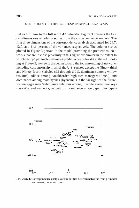
Let us turn now to the full set of 42 networks. Figure 3 presents the firsttwo dimensions of column scores from the correspondence analysis. Thefirst three dimensions of the correspondence analysis accounted for 24.7,12.9, and 11.1 percent of the variance, respectively. The column scoresplotted in Figure 3 pertain to the model providing the predictions. Net-works that are in close proximity in this figure are similar in the extent towhich their p* parameter estimates predict other networks in the set. Look-ing at Figure 3, we see in the center toward the top a grouping of networksincluding cosponsorship in all of the U.S. senates except the Ninety-thirdand Ninety-fourth~labeled s95 through s101!, dominance among willowtits ~tits!, advice among Krackhardt’s high-tech managers~krack!, anddominance among male hyenas~hyenam!. On the far right of the figure,we see aggressive0submissive relations among juvenile vervet monkeys~vervet1a and vervet2a, vervet2m!, dominance among sparrows~spar-

FIGURE 3. Correspondence analysis of similarities between networks from p*modelparameters, column scores.


row!, threats among highland ponies~ponies!, pant-grunt calls betweenchimpanzees~chimp1!, and patas monkeys fighting~patasf!.

In Figure 3 networks that are close to one another tend to exhibitsimilar structural properties. How can we interpret the overall spatial pat-terning in this figure? First, we use information about the structural fea-tures of the networks themselves, as seen in the directions and magnitudesof their p* parameter estimates. For each network, we code it as positive,negative, or none on each of the structural features based on the directionand nominal significance of the estimated coefficient for that property, asdescribed above. Table 1 reports these codings for each network as the p*

parameter profile. For example, we can see that the Ninety-third Senatehas positive tendencies for transitive triples, out-stars, and in-stars and anegative tendency for cyclic triples. We then draw confidence ellipsesaround the networks with each property on the correspondence analysisconfiguration.2 The results for mutuality, transitivity, and cycles are pre-sented in Figures 4 through 6.

We examine the extent to which networks with specific structuraltendencies occupy distinct regions of the correspondence space using ananalysis of variance with the dimension scores as the dependent variablesand the three category classifications of structural tendencies as factors,using the procedure described in Kumbasar, Romney, and Batchelder~1994! and Romney, Batchelder, and Brazill~1995!. An analysis of vari-ance comparing column dimension scores along the first three dimen-sions between three categories of structural properties gives the proportionreduction in error~PRE! in dimension scores due to the categorical group-ing variables, as measured by the correlation ratio squared,h2. Table 5presents these statistics for the first three dimensions of the correspon-dence analysis. From these results it is clear that the first dimension dis-tinguishes networks in which mutuality is an important property from thosein which it is not, or in which there is a tendency away from mutuality~h2 5 0.43!. Transitivity is an important contrast along the second dimen-sion~h2 5 0.27!.

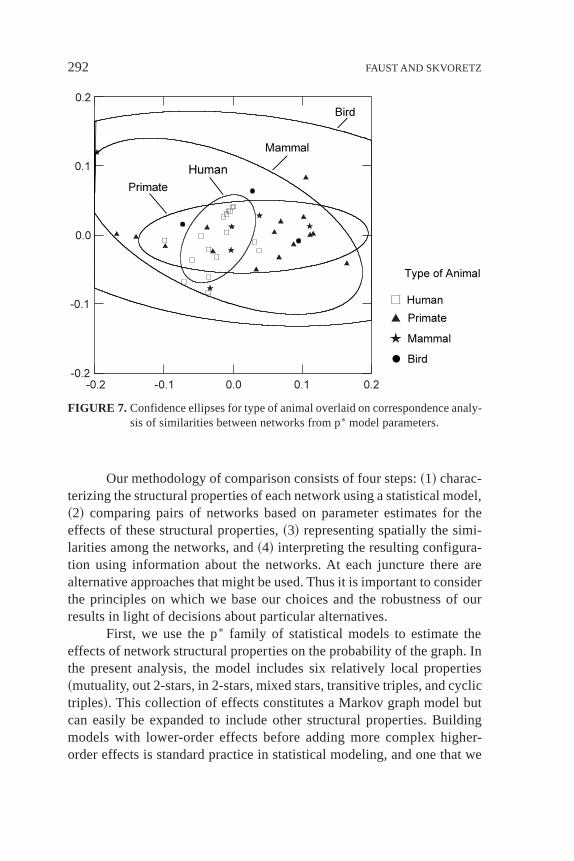
We use the same procedure to study whether similarities amongnetworks are patterned by animal type~human, nonhuman primate, non-primate mammal, or bird! or by relation type~observed positive, observednegative, reported positive, reported negative!. The confidence ellipses

2The confidence ellipse is centered on the means of the dimension 1 and dimen-sion 2 coordinates. Its orientation is determined by the covariance of the two vari-ables. We present 68.27 percent confidence ellipses.


for animal type and for relation type, overlaid on the correspondenceanalysis configurations, are in Figures 7 and 8. Results in Table 5 showthat the kind of animal is not an important distinction along any of thefirst three dimensions of the correspondence analysis. Whether the rela-tion is observed or reported is important along both of the first twodimensions~h2 5 0.10 andh2 5 0.20!, and whether the relation is pos-itive or negative is an important distinction along the first and thirddimensions~h2 5 0.12 andh2 5 0.13!. Relation type, coded into fourcategories, is an important aspect of the second dimension~h2 5 0.26!.Overall the type of relation appears to be more important than the typeof animal in distinguishing among the networks.

Further investigation of the associations between the relation typeand properties of the networks reveals some interesting relationships forour sample of networks. Observed positive relations~for example, groom-ing between nonhuman primates and cosponsorship between senators! tend

FIGURE 4. Confidence ellipses for mutuality overlaid on correspondence analysis ofsimilarities between networks from p* model parameters.


to be mutual, as do reported negative relations~blame and negative influ-ence!. In general, transitivity is characteristic of observed positive rela-tions, and a tendency away from transitivity is characteristic of reportednegative relations. Whether these associations hold in larger samples ofnetworks is a topic for future research.

7. DISCUSSION

We have described a methodology for comparing networks from diversesettings including vastly different species and relational contents. Thismethodology allows one to assess not only what structural features areimportant in a given network but also how similar various networks are interms of these properties. Important features of our approach are the cal-culation of an index of~dis!similarity between each pair of networks, and

FIGURE 5. Confidence ellipses for transitivity overlaid on correspondence analysisof similarities between networks from p* model parameters.


then the representation of these similarities among the diverse networksusing correspondence analysis. Information about characteristics of thenetworks, including the kinds of actors and types of relations, is then usedto interpret this spatial configuration.

In our results it appears that the kind of relation involved ratherthan the species underlies similarities among the networks. It is the natureof relation that determines the structural features of its network. For exam-ple, agonistic relations, whether between red deer or highland ponies, aresimilarly structured. This leads to the speculation that distinctions amongspecies in network structures are due to differences in the distributions ofrelations in which they typically engage. This also naturally suggests thatgreater efforts should be devoted to measuring the typical range of rela-tions for a species. For example, it would be useful to have observationaldata on different kinds of human interactions~though interviewing chim-panzees about who they go to for advice is probably out of the question!.

FIGURE 6. Confidence ellipses for cyclic triples overlaid on correspondence analy-sis of similarities between networks from p* model parameters.


TABLE 5Proportion Reduction in Error Measures~h2! for Correspondence Analysis Dimensions by Network Structural Properties, Type of

Animal, and Type of Relation

Dimension MutualaTransitiveTriplesa

CyclicTriplesa

Type ofAnimalb

Observed orReported Relation

Positive orNegative Relation

Type ofRelationc

1 0.43** 0.00 0.09 0.09 0.10* 0.12* 0.192 0.01 0.27** 0.00 0.05 0.20** 0.00 0.26*3 0.03 0.10 0.13 0.16 0.02 0.13* 0.14

*p , .05**p , .01aMutual, transitive, and cycle coded: positive, none, negative.bHuman, nonhuman primate, non-primate mammal, bird.cObserved positive, observed negative, reported positive, reported negative.

29

1

Our methodology of comparison consists of four steps:~1! charac-terizing the structural properties of each network using a statistical model,~2! comparing pairs of networks based on parameter estimates for theeffects of these structural properties,~3! representing spatially the simi-larities among the networks, and~4! interpreting the resulting configura-tion using information about the networks. At each juncture there arealternative approaches that might be used. Thus it is important to considerthe principles on which we base our choices and the robustness of ourresults in light of decisions about particular alternatives.

First, we use the p* family of statistical models to estimate theeffects of network structural properties on the probability of the graph. Inthe present analysis, the model includes six relatively local properties~mutuality, out 2-stars, in 2-stars, mixed stars, transitive triples, and cyclictriples!. This collection of effects constitutes a Markov graph model butcan easily be expanded to include other structural properties. Buildingmodels with lower-order effects before adding more complex higher-order effects is standard practice in statistical modeling, and one that we

FIGURE 7. Confidence ellipses for type of animal overlaid on correspondence analy-sis of similarities between networks from p* model parameters.


follow here. In addition, there are alternatives to the p* modeling frame-work that also could be used to estimate effects of network structuralproperties—for example, Friedkin’s local density model~Friedkin 1998!could be used to estimate tie probabilities.

The second step is to compare networks based on the structuralparameters in the models. We base our choice here on the principle thatnetworks of different sizes and of different densities can have similarstructures. We view size and density as differences of scale rather thanas differences of theoretical significance. This leads us to use standard-ized regression coefficients and standardized explanatory variables forpredicting tie probabilities. Comparison is then based on predicted tieprobabilities, using a network’s own parameter estimates and the param-eter estimates from other networks. Resemblance between networks ismeasured using Euclidean distance. Other measures of similarity~suchas a correlation coefficient! would also be possible. We have exploredother modes of comparison, using predicted probabilities from unstan-dardized regression coefficients, and using predicted logits rather than

FIGURE 8. Confidence ellipses for type of relation overlaid on correspondence analy-sis of similarities between networks from p* model parameters.


predicted probabilities. In all cases the results and substantive conclu-sions are substantially similar to those we present here. We have onlypreliminarily explored another alternative—namely, direct comparisonof the parameter estimates themselves. Our preliminary investigation onthe current data indicates this comparison would yield the same substan-tive conclusions.

The third step in our methodology represents spatially the~dis!sim-ilarities among the collection of networks. Since the matrix of~dis!simi-larities is not symmetric we use correspondence analysis rather than otherscaling options that require symmetric input data. Finally, we interpret theresulting configuration of similarities among networks by systematicallyexamining which features of the networks are related to the spatial con-figuration from the correspondence analysis.

This research may be extended in several directions. First, themethod can easily be used to compare multiple networks in a wide vari-ety of situations. For example, one could compare friendship networksin multiple schools, communications relations in multiple organiza-tions, or interorganizational transactions in multiple communities. Thusour method can be used to address fundamental questions about variabil-ity or similarity in network structure and organization. Importantly, how-ever, our methodology is not restricted to comparing networks wherethe same relation has been measured in all settings. Second, in futureresearch it will be important to explore two extensions to the modelsfor tie probabilities or strengths. The first extension would handle val-ued relations. In this paper, we have, perhaps somewhat arbitrarily,dichotomized all relations. The second extension would include addi-tional structural features in the p* models used to characterize the net-works. We have used a limited set of relatively local properties in ourmodels. Certainly graph-level properties, such as network centraliza-tion, the diameter of the graph, or the average path length between pointscould also be included. Theoretically, the addition of these long-rangeeffects may prove quite interesting if it turns out that they have differ-ent impacts in the networks of humans as opposed to the networks ofother animals.

APPENDIX: LIST OF DATA SOURCES

This appendix lists the 42 networks, describes the relations, gives a refer-ence for the source of the data, and reports the label used in Table 1 and


Figure 2. Where data are published, the table number and page of thesource are given. Numbers correspond to numbers listed in Table 1.

• 1–9.U.S. Senate. Cosponsorship in nine senates. Records whether sen-ator i cosponsored at least one bill introduced by senatorj during thatsession of the Senate. Data provided by Burkett~1997!. Labels: s93,s94, s95, s96, s97, s98, s99, s100, s101.

• 10. Krackhardt’s high-tech managers. Each manager was asked whothey went to for help or advice at work; Krackhardt~1987!. Data avail-able in Wasserman and Faust~1994! and in UCINET~Borgatti, Everett,and Freeman 1999!. Label: krack.

• 11–14.Sampson’s monastery. Four relations reported between monks inthe monastery: positive influence~Table D15, p. 471!, negative influ-ence ~Table D15, p. 471!, blame ~Table D16, p. 472!, and praise~Table D16, p. 472!; data from Sampson~1968!. Data are also availablein UCINET ~Borgatti, Everett, and Freeman 1999!. Labels: sampin,sampnin, sampnpr, samppr.

• 15–18.Athanassiou and Nigh’s top management teams (TMT). Thereare two teams~02 and 05!and two relations: from whom each managersought advice and how extensively they had worked together; Athanas-siou and Nigh~1999!. Data provided by the second author. Labels: ua02,ua05~advice!, ue02, ue05~work with!.

• 19–21.Chimpanzees. Three relations: pant-grunt calls~Table 9.3, p. 119!,initiation of dyadic agonistic confrontations~Table 9.4, p. 119!, and ini-tiation of grooming~Table 9.14a, p. 126!; data from Nishida and Hosaka~1996!. Labels: chimp1, chimp2, and chimp3.

• 22.Macaca Mulatta. One relation: grooming~Table 1, p. 274!; data arefrom Sade~1989!. Label: macaca.

• 23–26.Macaques, macaca sylvanus.Four relations: male carried babyaway from another~Table 7a, p. 71!, label macaqa; male left anotherwith a baby~Table 7b, p. 71!, label macaqb; male carrying a babyapproached another male~Table 5a, p. 69!, label macaqc; maleapproached another male who was with a baby~Table 5b, p. 69!, labelmacaqd; data from Deag~1980!.

• 27. Stumptail Macaques~Macaca artaides!. The relation is aggression~Table 2, p. 247!; data are from Dow and de Waal~1989!. Label: macaqu.

• 28–29.Patas monkeys. Two relations: fighting~Table III, p. 202! andgrooming~Table V, p. 205!; data from Kaplan and Zucker~1980!. Labels:pataf and patag.


• 30–33.Vervet monkeys~Cercopithecus aethiops sabaeus!, juveniles fromtwo troops~1 and 2! and two conditions~mother present and motherabsent!: dyadic aggressive0submissive interactions, both mothers present~Table I, p. 775!, labels: vervet1m and vervet2m; dyadic aggressive0submissive interactions, both mothers absent~Table II, p. 776!, labels:vervet1a and vervet2a; data from Horrocks and Hunte~1983!.

• 34–35.Cows, bos indicus. Two relations: social licking~Figure 7, p. 130!and social grazing~Figure 4, p. 126!; data from Reinhardt and Rein-hardt~1981!. Labels: cowl, cowg.

• 36–37.Hyaena, crocuta crocuta.Dominance, among females and amongmales. Dominance among adult females~Table I, p. 1513! and domi-nance among males~Table V, p. 1519!; data from Frank~1986!. Labels:hyenaf, hyenam.

• 38. Highland ponies. The relation is threats~Table 2, p. 3!; data fromRoberts and Browning~1998!, originally in Clutton-Brock, Green-wood, and Powell~1976!. Label: ponies.

• 39. Red deer stags, Cervus elaphus L.Winner and loser in encounters~Figure 1~a!, p. 601!; data from Appleby~1983! and also in Freeman,Freeman, and Romney~1992! and Roberts~1994!. Label: reddeer.

• 40.Silvereyes, zosterops lateralis.One relation, victories in encounters~Table 1, p. 94!; data from Kikkawa~1980!. Label: silver.

• 41.Sparrows, zonotrichia querula.One relation: dominance, both attacksand avoidances~Figure 2, p. 19!; data from Watt~1986!. Label: sparrow.

• 42. Willow tits, parus montanus. One relation: dominance~Table 1,p. 1492!; data from Tufto, Solberg, and Ringgsby~1998!. Data origi-nally from Lahti, Koivula, and Orell~1994!. Label: tits.

REFERENCES

Appleby, Michael. 1983. “The Probability of Linearity in Hierarchies.”Animal Behav-iour 31:600–608.

Anderson, Carolyn, J., Stanley Wasserman, and Bradley Crouch. 1999. “A p* Primer:Logit Models for Social Networks.”Social Networks21:37–66.

Athanassiou, Nicholas, and Douglas Nigh. 1999. “The Impact of U.S. Company Inter-nationalization on Top Management Team Advice Networks: A Tacit KnowledgePerspective.”Strategic Management Journal20:83–92.

Baker, Frank, and Lawrence Hubert. 1981. “The Analysis of Social Interaction Data.”Sociological Methods and Research9:339–61.

Bearman, P. S., J. Jones, and J. R. Udry. 1997. “National Longitudinal Study of Ado-lescent Health: Research Design.” Carolina Population Center. Unpublishedmanuscript.


Bernard, H. Russell, and Peter D. Killworth. 1977. “Informant Accuracy in SocialNetwork Data II.”Human Communications Research4:3–18.

Bernard, H. Russell, Peter D. Killworth, and Lee D. Sailer. 1980. “Informant Accu-racy in Social Network Data IV: A Comparison of Clique-Level Structure in Behav-ioral and Cognitive Network Data.”Social Networks2:191–218.

Borgatti, Stephen, Martin Everett, and Linton Freeman. 1999. UCINET 5.0 for Win-dows. Analytic Technologies.

Breiger, R. L., and P. Pattison. 1978. “The Joint Role Structure of Two Communities’Elites.” Sociological Methods and Research7:213–26.

Burkett, Tracy. 1997. “Cosponsorship in the United States Senate: A Network Analy-sis of Senate Communication and Leadership, 1973–1990.” Ph.D. dissertation. Uni-versity of South Carolina.

Carroll, J. Douglas, Ece Kumbasar, and A. Kimball Romney. 1997. “An EquivalenceRelation Between Correspondence Analysis and Classical Multidimensional Scal-ing for the Recovery of Euclidean Distances.”British Journal of Mathematicaland Statistical Psychology50:81–92.

Clutton-Brock, T. H., P. J. Greenwood, and R. P. Powell. 1976. “Ranks and Relation-ships in Highland Ponies and Highland Cows.”Z. Tierpsychol41:202–16.

Crouch, Bradley, and Stanley Wasserman. 1998. “A Practical Guide to Fitting p* SocialNetwork Models.”Connections21:87–101.

Davis, James A. 1979. “The Davis0Holland0Leinhardt Studies: An Overview.” Pages51–62 inPerspectives on Social Network Research, edited by Paul W. Holland andSamuel Leinhardt. New York: Academic Press.

Deag, John M. 1980. “Interactions Between Males and Unweaned Barbary Macaques:Testing the Agonistic Buffering Hypothesis.”Behaviour75:54–81.

Dow, Malcolm M., and Frans B. M. de Waal. 1989. “Assignment Methods for theAnalysis of Network Subgroup Interactions.”Social Networks11:237–55.

Frank, Ove, and David Strauss. 1986. “Markov Graphs.”Journal of the AmericanStatistical Association81:832–42.

Frank, Laurence G. 1986. “Social Organization of the Spotted Hyaena Crocuta Cro-cuta. II: Dominance and Reproduction.”Animal Behaviour34:1510–27.

Freeman, Linton. 1992. “The Sociological Concept of ‘Group’: An Empirical Test ofTwo Models.”American Journal of Sociology98:152–66.

Freeman, Linton C., Sue C. Freeman, and A. Kimball Romney. 1992. “The Implica-tions of Social Structure for Dominance Hierarchies in Red Deer.”Animal Behav-iour 44:239–45.

Friedkin, Noah. 1998.A Structural Theory of Social Influence. Cambridge, UK: Cam-bridge University Press.

Gifi, Albert. 1990.Nonlinear Multivariate Analysis. New York: Wiley.Greenacre, Michael. 1984.Theory and Applications of Correspondence Analysis. New

York: Academic Press.Hallinan, Maureen T. 1974. “A Structural Model of Sentiment Relations.” American

Journal of Sociology80:364–78.Holland, Paul W., and Samuel Leinhardt. 1978. “An Omnibus Test for Social Structure

Using Triads.”Sociological Methods and Research7:227–56.Horrocks, Julia, and Wayne Hunte. 1983. “Maternal Rank and Offspring Rank in Vervet


Monkeys: An Appraisal of the Mechanisms of Rank Acquisition.”Animal Behav-iour 31:772–82.

Hubert, Lawrence, and Frank Baker. 1978. “Evaluating the Conformity of Sociomet-ric Measurements.”Psychometrika43:31–41.

Johnson, Jeffrey C., James S. Boster, and Lawrence Palinkas. n.d. “The Evolution ofNetworks in Extreme and Isolated Environments.” Unpublished manuscript.

Kaplan, J. R., and E. Zucker. 1980. “Social Organization in a Group of Free-rangingPatas Monkeys.”Folia Primatologica34:196–213.

Katz, Leo, and James H. Powell. 1953. “A Proposed Index of the Conformity of OneSociometric Measurement to Another.”Psychometrika18:249–56.

Kikkawa, Jiro. 1980. “Weight Change in Relation to Social Hierarchy in Captive Flocksof Silvereyes, Zosterops Lateralis.” Behaviour74:92–100.

Krackhardt, David. 1987. “Cognitive Social Structures.”Social Networks9:104–34.Kumbasar, Ece, A. Kimball Romney, and William H. Batchelder. 1994. “Systematic

Biases in Social Perception.”American Journal of Sociology100:477–505.Lahti, K., K. Koivula, and M. Orell. 1994. “Is the Social Hierarchy Always Linear in

Tits.” Journal of Avian Biology25:347–48.Laumann, E. O., and F. Pappi. 1976.Networks of Collective Action: A Perspective on

Community Influence Systems. New York: Academic Press.Martin, John. 1999. “A General Permutation-Based QAPAnalysis Approach for Dyadic

Data from Multiple Groups.”Connections22:50–60.Maryanski, A. P. 1987. “African Ape Social Structure: Is There Strength in Weak Ties?”

Social Networks9:191–215.Nishida, Toshisada, and Kasuhiko Hosaka. 1996. “Coalition Strategies Among Male

Chimpanzees of the Mahale Mountains, Tanzania.” Pp. 114–134 inGreat Ape Soci-eties, edited by William C. McGrew, Linda F. Marchant, and Toshisada Nishida.New York: Cambridge University Press.

Nishisato, Shizuhiko. 1994.Elements of Dual Scaling: An Introduction to PracticalData Analysis. Hillsdale, NJ: Lawrence Erlbaum.

Pattison, Philippa, and Stanley Wasserman. 1999. “Logit Models and Logistic Regres-sions for Social Networks: II. Multivariate Relations.”British Journal of Math-ematical and Statistical Psychology52:169–93.

Reinhardt, Viktor, and Annie Reinhardt. 1981. “Cohesive Relationships in a CattleHerd~Bos Indicus!.” Behaviour76:121–51.

Rindfuss, Ronald R., Aree Jampaklay, Barbara Entwisle, Yothin Sawangdee, KatherineFaust, and Pramote Prasartkul. 2000. “The Collection and Analysis of Social Net-work Data in Nang Rong, Thailand.” Presented at the IUSSP Conference on Part-nership Networks, February, Chiang Mai, Thailand.

Roberts, John M., Jr. 1994. “Fit of Some Models to Red Deer Dominance Data.”Jour-nal of Quantitative Anthropology4:249–58.

Roberts, John M., Jr., and Bridget A. Browning. 1998. “Proximity and Threats in High-land Ponies.”Social Networks20:227–38.

Robins, Garry, Philippa Pattison, and Stanley Wasserman. 1999. “Logit Models andLogistic Regressions for Social Networks. III. Valued Relations.”Psychometrika64:371–94.

Romney, A. Kimball, William H. Batchelder, and Timothy Brazill. 1995. “Scaling


Semantic Domains.” Pp. 267–94 inGeometric Representations of Perceptual Phe-nomena: Papers in Honor of Tarow Indow’s 70th Birthday, edited by Duncan Luceet al. Hillsdale, NJ: Lawrence Erlbaum.

Sade, Donald Stone. 1989. “Sociometrics ofMacaca MulattaIII: N-path Centrality inGrooming Networks.”Social Networks11:273–92.

Sade, Donald Stone, and Malcolm Dow. 1994. “Primate Social Networks.” Pp. 152–66in Advances in Social Network Analysis, edited by Stanley Wasserman and JosephGalaskiewicz. Thousand Oaks: Sage.

Sampson, S. 1968. “A Novitiate in a Period of Change: An Experimental and CaseStudy of Social Relationships.” Ph.D. dissertation. Cornell University.

Shrader, Charles B., James R. Lincoln, and Alan N. Hoffman. 1989. “The NetworkStructures of Organizations: Effects of Task Contingencies and Distributional Form.”Human Relations42:43–66.

Snijders, T. A. B. 1996. “Stochastic Actor-Oriented Dynamic Network Analysis.”Jour-nal of Mathematical Sociology21:149–72.

Snijders, T. A. B., and M. A. J. Van Duijn. 1997. “Simulation for Statistical Inferencein Dynamic Network Models.” Pp. 493–512 inSimulating Social Phenomena, editedby R. Conte, R. Hegselmann, and P. Terna. Berlin: Springer.

Strauss, David, and Michael Ikeda. 1990. “Pseudolikelihood Estimation for SocialNetworks.”Journal of the American Statistical Association85:204–12.

Tufto, Jarle, Erling Johan Solberg, and Thor-Harald Ringgsby. 1998. “Statistical Mod-els of Transitive and Intransitive Dominance Structures.”Animal Behaviour55:1489–98.

Wasserman, Stanley. 1987. “Conformity of Two Sociometric Relations.”Psychometrika52:3–18.

Wasserman, Stanley, and Katherine Faust. 1994.Social Network Analysis: Methodsand Applications. Cambridge, England: Cambridge University Press.

Wasserman, Stanley, and Dawn Iacobucci. 1988. “Sequential Social Network Data.”Psychometrika53:261–82.

Wasserman, Stanley, and Philippa Pattison. 1996. “Logit Models and Logistic Regres-sions for Social Networks: I. An Introduction to Markov Graphs and p*.” Psy-chometrika61:401–25.

Watt, Doris, J. 1986. “Relationship of Plumage Variability, Size, and Sex to SocialDominance.”Animal Behaviour34:16–27.

Weller, Susan C., and A. Kimball Romney. 1990.Metric Scaling: CorrespondenceAnalysis. Newbury Park, CA: Sage.


Comparing Networks Across Space and Time, Size and Species

Documents

Transcript of Comparing Networks Across Space and Time, Size and Species