Atmos. Meas. Tech., 11, 3955–3967, 2018https://doi.org/10.5194/amt-11-3955-2018© Author(s) 2018. This work is distributed underthe Creative Commons Attribution 4.0 License.

Comparing OMI-based and EPA AQS in situ NO2 trends: towardsunderstanding surface NOx emission changesRuixiong Zhang1, Yuhang Wang1, Charles Smeltzer1, Hang Qu1, William Koshak2, and K. Folkert Boersma3,4

1School of Earth and Atmospheric Sciences, Georgia Institute of Technology, Atlanta, Georgia, USA2NASA-Marshall Space Flight Center, National Space Science & Technology Center,320 Sparkman Drive, Huntsville, Alabama, USA3Meteorology and Air Quality Group, Wageningen University, Wageningen, the Netherlands4Royal Netherlands Meteorological Institute, De Bilt, the Netherlands

Correspondence: Yuhang Wang (yuhang.wang@eas.gatech.edu)

Received: 13 November 2017 – Discussion started: 25 January 2018Revised: 22 June 2018 – Accepted: 26 June 2018 – Published: 6 July 2018

Abstract. With the improved spatial resolution of the OzoneMonitoring Instrument (OMI) over earlier instruments andmore than 10 years of service, tropospheric NO2 retrievalsfrom OMI have led to many influential studies on the rela-tionships between socioeconomic activities and NOx emis-sions. Previous studies have shown that the OMI NO2 datashow different relative trends compared to in situ measure-ments. However, the sources of the discrepancies need fur-ther investigations. This study focuses on how to appropri-ately compare relative trends derived from OMI and in situmeasurements. We retrieve OMI tropospheric NO2 verticalcolumn densities (VCDs) and obtain the NO2 seasonal trendsover the United States, which are compared with coinci-dent in situ surface NO2 measurements from the Air Qual-ity System (AQS) network. The Mann–Kendall method withSen’s slope estimator is applied to derive the NO2 seasonaland annual trends for four regions at coincident sites dur-ing 2005–2014. The OMI-based NO2 seasonal relative de-creasing trends are generally biased low compared to the insitu trends by up to 3.7 % yr−1, except for the underestima-tion in the US Midwest and Northeast during December, Jan-uary, and February (DJF). We improve the OMI retrievals fortrend analysis by removing the ocean trend, using the Moder-ate Resolution Imaging Spectroradiometer (MODIS) albedodata in air mass factor (AMF) calculation. We apply a light-ning flash filter to exclude lightning-affected data to makeproper comparisons. These data processing procedures re-sult in close agreement (within 0.3 % yr−1) between in situand OMI-based NO2 regional annual relative trends. The re-

maining discrepancies may result from inherent differencebetween trends of NO2 tropospheric VCDs and surface con-centrations, different spatial sampling of the measurements,chemical nonlinearity, and tropospheric NO2 profile changes.We recommend that future studies apply these procedures(ocean trend removal and MODIS albedo update) to ensurethe quality of satellite-based NO2 trend analysis and applythe lightning filter in studying surface NOx emission changesusing satellite observations and in comparison with the trendsderived from in situ NO2 measurements. With these data pro-cessing procedures, we derive OMI-based NO2 regional an-nual relative trends using all available data for the US West(−2.0 %± 0.3 yr−1), Midwest (−1.8 %± 0.4 yr−1), North-east (−3.1 %± 0.5 yr−1), and South (−0.9 %± 0.3 yr−1).The OMI-based annual mean trend over the contiguousUnited States is −1.5 %± 0.2 yr−1. It is a factor of 2 lowerthan that of the AQS in situ data (−3.9 %± 0.4 yr−1); thedifference is mainly due to the fact that the locations of AQSsites are concentrated in urban and suburban regions.

1 Introduction

Nitrogen dioxide (NO2) is an air pollutant. At high concen-trations, it aggravates respiratory diseases and can lead toacid rain formation (e.g., Lamsal et al., 2015). It is also a keyplayer in producing another pollutant, ozone (O3), throughphotochemical reactions in the presence of volatile organiccompounds (VOCs) in sunlight. Tropospheric NO2 is emitted

Published by Copernicus Publications on behalf of the European Geosciences Union.

3956 R. Zhang et al.: Comparing OMI-based and EPA AQS in situ NO2 trends

both anthropogenically and naturally (e.g., Gu et al., 2016).Anthropogenic fossil fuel combustions and biomass burningemit mostly nitrogen monoxide (NO) at high temperature,which is later oxidized by O3 into NO2. Major natural NO2sources include lightning and soils.

Surface NO2 concentrations are regulated by the US En-vironmental Protection Agency (EPA) through the NationalAmbient Air Quality Standards (NAAQS). NO2 is measuredroutinely at the EPA Air Quality System (AQS) sites (Demer-jian, 2000). Although the AQS network continually providesvaluable hourly NO2 measurements, AQS sites are mostly lo-cated in urban and suburban regions, leaving large regions ofrural areas unmonitored. Satellite data provide better spatialcoverage than the in situ measurements.

Several satellites have been launched to monitor tropo-spheric NO2 vertical column densities (VCDs), such asthe SCanning Imaging Absorption spectroMeter for Atmo-spheric CHartographY (SCIAMACHY), the Global OzoneMonitoring Experiment–2 (GOME-2), and the Ozone Moni-toring Instrument (OMI). For trend analysis, the troposphericNO2 products from OMI surpass the others for a relativelyhigh spatial resolution and over 1 decade of continuous op-eration (Boersma et al., 2004, 2011). Thus, OMI NO2 re-trievals are widely applied in NO2 and NOx emission trendstudies (e.g., Lin et al., 2010, 2013; Lin and McElroy, 2011;Castellanos and Boersma, 2012; Russell et al., 2012; Gu etal., 2013; Lamsal et al., 2015; Lu et al., 2015; Tong et al.,2015; Cui et al., 2016; Duncan et al., 2016; de Foy et al.,2016a, b; Krotkov et al., 2016; Liu et al., 2017). Tong etal. (2015) reported that the reduction rates calculated fromOMI NO2 VCDs and AQS surface NO2 data in eight citieswere −35 and −38 % from 2005 to 2012, respectively. Lam-sal et al. (2015) also found the divergence between the an-nual trends inferred from the two datasets, i.e., −4.8 % yr−1

vs. −3.7 % yr−1 during 2005–2008, and −1.2 % yr−1 vs.−2.1 % yr−1 during 2010–2013. There are several potentialfactors that contribute to the discrepancies between trendsfrom satellite and ground-based measurements: interferencesby the oxidation products of NOx from the chemilumines-cent instruments (Lamsal et al., 2008, 2014, 2015), the dif-ferences of sampling time between OMI (∼ 13:30 local time)and AQS (hourly) measurements (Tong et al., 2015), a highsensitivity of NO2 VCDs to high-altitude NO2 in contrast tothe high sensitivity of surface NO2 concentrations to surfaceNOx emissions (Duncan et al., 2013; Lamsal et al., 2015),spatial representativeness of satellite pixels (Lamsal et al.,2015), and high uncertainties of satellite retrievals in cleanregions (Lamsal et al., 2015).

To understand how various factors and the retrieval proce-dure affect the differences between the OMI-derived trendsand those derived from the surface AQS measurements, weutilize a regional 3-D chemistry transport model (CTM),a radiative transfer model (RTM), and the Mann–Kendallmethod (Mann, 1945; Kendall, 1948) to calculate OMI-basedNO2 seasonal relative trends during December, January, and

February (DJF); March, April, and May (MAM); June, July,and August (JJA); and September, October, and November(SON) (Sect. 2). We find that two procedures are essential toensure the quality of trend analysis using OMI troposphericNO2 VCDs, including the ocean trend removal and theModerate Resolution Imaging Spectroradiometer (MODIS)albedo update in calculating the air mass factors (AMFs).The lightning filter (Sect. 3.1) is necessary for comparingOMI-based and in situ AQS NO2 trends. With these proce-dures implemented, the differences between OMI-based andAQS in situ annual relative trends are within 0.3 % yr−1 ofcoincident measurements for all the four regions. Finally, weestimate the OMI-based annual relative trends across the na-tion in Sect. 3.2. Conclusions are given in Sect. 4.

2 Methods

2.1 EPA AQS surface NO2 measurements

The in situ surface NO2 measurements from the US EPAAQS network are used in this research. Sites with a continu-ous measurement gap of more than 50 days are removed, andthe observations of 140 remaining cites are used (Fig. 1). TheAQS chemiluminescent analyzers are equipped with molyb-denum converters to measure ambient NO2 concentrations.These analyzers are known to have high biases, since the con-verters are not NO2 specific and they measure some fractionsof peroxyacetyl nitrate, nitric acid, and organic nitrates (De-merjian, 2000; Lamsal et al., 2008). In addition to chemi-luminescent analyzers, several NO2-specific photolytic in-struments have been deployed since 2013. By utilizing thedata from both chemiluminescent and photolytic measure-ments at coincident sites during the overpassing time of OMI,we calculate the observed NO2 concentration ratio betweenboth measurements in Fig. S1 in the Supplement. The ratiopeaks at 2.3 in June and decreases to 1.3 in November, indi-cating that the chemiluminescent analyzers overestimate by27–132 % as compared to photolytic instruments. This find-ing is in agreement with Lamsal et al. (2008). We correct thechemiluminescent NO2 data by the observed ratio, assum-ing that the interannual change is small and the high bias ofthe chemiluminescent measurements is identical at all sites.This correction may contribute to the differences between insitu and OMI-based absolute NO2 trends but does not signif-icantly affect the relative trends (since the correction is can-celed out in computing relative trends). In this study, we onlyexamine the relative trends, and therefore the analysis resultsare not affected by the uncertainties in the in situ NO2 mea-surement corrections.

2.2 REAM model

We use the 3-D Regional chEmical trAnsport Model(REAM) in the simulation of NO2 profiles. REAM haswidely been used in atmospheric NO2 studies, including ver-

Atmos. Meas. Tech., 11, 3955–3967, 2018 www.atmos-meas-tech.net/11/3955/2018/

R. Zhang et al.: Comparing OMI-based and EPA AQS in situ NO2 trends 3957

Figure 1. The solid black borders in the center map define the four regions used in this study. The colored background shows the OMI-basedNO2 annual relative trends of the “lightning filter” data. Grid cells with 2005–2014 mean NO2 VCD values < 1× 1015 molecules cm−2 areexcluded in this study and are shown in white. The black-bordered circles represent the locations of AQS sites. Panel (a) through (d) showthe regional difference (OMI-based relative trends minus AQS relative trends) of annual relative trends between coincident OMI-based andAQS in situ data. The colored diamonds are for “standard” (orange), “ocean” (blue), “MODIS” (green), and “lightning filter” (red) OMI data.The different OMI VCD data are described in Sect. 2.4.

tical transport (Choi et al., 2005; Zhao et al., 2009; Zhang etal., 2016), emission inversions (Zhao and Wang, 2009; Yanget al., 2011; Gu et al., 2013, 2014, 2016), and regional andseasonal variations (Choi et al., 2008a, b). The model hasa horizontal resolution of 36 km with 30 vertical layers inthe troposphere, 5 vertical layers in the stratosphere, and amodel top of 10 hpa. In this study, the domain of REAM isabout 400 km larger on each side than the contiguous UnitedStates (CONUS). Meteorology inputs driving the transportprocess are simulated by the Weather Research and Fore-casting model (WRF) assimilations constrained by NationalCenters for Environmental Prediction Climate Forecast Sys-tem Reanalysis (NCEP CFSR; Saha et al., 2010) 6-hourlyproducts. The KF-Eta scheme is used for sub-grid convectivetransport in WRF (Kain and Fritsch, 1993). We run the WRFmodel with the same resolution as in REAM but with a do-main 10 grids larger on each side than that of REAM. REAMupdates most of the meteorology inputs every 30 min, whilethose related to convective transport and lightning parameter-ization are updated every 5 min. The chemistry mechanismexpands upon that of the global CTM GEOS-Chem (V9-02)with aromatic chemistry (Bey et al., 2001; Liu et al., 2010,2012a, b; Zhang et al., 2017). For consistency, the GEOS-Chem (V9-02) simulation with 2◦× 2.5◦ resolution is usedto generate initial and boundary conditions for chemical trac-ers.

Anthropogenic emissions of NOx and other chemicalspecies are from the US National Emission Inventory 2008prepared using the Sparse Matrix Operator Kernel Emission(SMOKE) model. Biogenic emissions are simulated online

using the Model of Emissions of Gases and Aerosols fromNature (MEGAN) algorithm (v2.1; Guenther et al., 2012).We parameterize lightning-emitted NOx as a function of con-vective mass flux and convective available potential energy(CAPE) (Choi et al., 2005). NOx production per flash is setto 250 moles NO per flash, and the emissions are distributedvertically following the C-shaped profiles by Pickering etal. (1998). For recent model evaluations of REAM with ob-servations, we refer readers to Zhang et al. (2016), Zhang andWang (2016), Cheng et al. (2017), and Zhang et al. (2017).

2.3 OMI-based NO2 VCDs

We retrieve the tropospheric NO2 VCDs using the tro-pospheric slant column densities (SCDs, without destrip-ing) from the Royal Dutch Meteorological Institute (KNMI)Dutch OMI NO2 product (DOMINO v2; Boersma et al.,2011). OMI on board the Aura satellite was launched in July2004 and is still active. OMI overpasses the Equator at about13:30 local time (LT) and obtains global coverage with a2600 km viewing swath spanning 60 rows. It has a groundlevel spatial resolution up to 13 km× 24 km (at nadir). Thespatial extent of the OMI pixels will not affect our analysisas we focus on regional trend analysis. SCDs are retrievedby matching a modeled spectrum to an observed top-of-atmosphere reflectance with the differential optical absorp-tion spectroscopy (DOAS) technique within a fitting win-dow of 405–465 nm. The stratospheric portion of SCDs isestimated and subsequently removed with the global CTMTM4 with stratospheric ozone assimilation (Dirksen et al.,2011). Deriving tropospheric VCDs from the remaining tro-

www.atmos-meas-tech.net/11/3955/2018/ Atmos. Meas. Tech., 11, 3955–3967, 2018

3958 R. Zhang et al.: Comparing OMI-based and EPA AQS in situ NO2 trends

pospheric SCDs requires the calculation of AMFs. SinceNO2 is an optically thin gas, tropospheric AMF for NO2can be calculated from AMF for each vertical layer (AMFl)weighted by NO2 partial VCDs at the corresponding layer(xl) (Boersma et al., 2004), as shown in Eq. (1).

troposphericAMF=troposphericSCDtroposphericVCD

=

∫AMFlxldl∫

xldl(1)

As the vertical distribution of NO2 is usually unknown, wetypically substitute xl by an a priori profile (xl, apriori) froma CTM. AMFl is the sensitivity of NO2 SCD to VCD at agiven altitude (Eskes and Boersma, 2003) and is computedusing the Double-Adding KNMI (DAK) RTM (Boersma etal., 2011). As a result, the retrieved tropospheric NO2 VCDcomputation depends on the a priori NO2 vertical profile,the surface reflectance, the surface pressure, the temperatureprofile, and the viewing geometry (Boersma et al., 2011).Previous studies have addressed the sources of uncertaintiesin NO2 retrievals, including surface reflectance resolutions(Russell et al., 2011; Lin et al., 2014), lightning NOx (Choiet al., 2005; Martin et al., 2007; Bucsela et al., 2010), a pri-ori CTM uncertainties (Russell et al., 2011; Heckel et al.,2011; Lin et al., 2012; Laughner et al., 2016), surface pres-sure and reflectance anisotropy in rugged terrain (Zhou et al.,2009), cloud and aerosol radiance (Lin et al., 2014, 2015),and boundary layer dynamics (Zhang et al., 2016). In thisstudy, we find that the first two factors are essential in NO2VCD trend analysis, and we will discuss these in the follow-ing sections.

AMFs are derived using the pre-computed altitude-dependent AMF lookup table, which is generated by theDAK RTM. We use the NO2 profiles from REAM, temper-ature and pressure from CSFR, and viewing geometry andcloud information from the DOMINO v2 product. We use theREAM results of 2010 to avoid the uncertainty introducedby yearly variation of NO2 profiles. The yearly variations ofmeteorology and anthropogenic emission changes have littleimpact in polluted areas on trend analysis results using OMIdata (Lamsal et al., 2015). We use the surface reflectancefrom the DOMINO v2 product as a default (Kleipool et al.,2008) and update it using a surface reflectance product witha higher temporal resolution (Sect. 2.3.2). The derived tro-pospheric NO2 VCD relative trends with default surface re-flectance are referred to as “standard”.

2.3.1 Ocean trend removal

For trend and other analyses of OMI tropospheric VCDs, thedata of anomalous pixels must be removed. The row anomalyinitially occurred in June 2007 and subsequently in lateryears affected rows 26–40 (Schenkeveld et al., 2017). Addi-tional anomalies can be found in some years in rows 41–55.For trend analysis from 2005 to 2014, we exclude rows 26–55, consistent with our understanding of the row anomaly(Schenkeveld et al., 2017). In addition, the data of coarse spa-

tial resolution from rows 1 to 5 and rows 56 to 60 are also ex-cluded, as suggested by Lamsal et al. (2015). The selectionof rows 6–25 used in this research is stricter than the dataflags in the DOMINO v2 product. Furthermore, we excludeOMI data with cloud fraction > 0.3 to minimize retrieval un-certainties due to clouds and aerosols (Boersma et al., 2011;Lin et al., 2014).

Figure 2a shows that there is an apparent increasing trendof the averaged tropospheric SCDs in the remote oceanregion (Fig. 2b) with minimal marine traffic. This trendmay reflect the inaccurately simulated stratospheric SCDsor the increase in the magnitude of the stripes (step-wiseSCD variability from one row to another) in time, whichoriginates from the use of a constant (2005-averaged) so-lar irradiance reference spectrum in the DOAS spectral fitsthroughout the mission and the weak increase of noisein the OMI radiance measurements (K. Folkert Boersma,personal communication, 2017; Zara et al., 2018). Fig-ure 2a shows that there is a positive annual trend of1.75± 0.45× 1013 molecules cm−2 yr−1. The ocean trend isinsensitive to the region selection in the remote North Pacific(varies within 10 %). We only analyze OMI tropospheric col-umn trends over the CONUS for grid cells with 2005–2014-averaged VCDs > 1× 1015 molecules cm−2, which tends tominimize the effect of the background noise. However, re-moving this background ocean (absolute) trend has a non-negligible effect in reducing the OMI relative trend (Fig. 1).We treat this trend as a systematic bias. We calculate the con-tribution from the ocean (absolute) annual trend to SCDs foreach year and subtract it from OMI tropospheric NO2 SCDsuniformly in the following analysis. Since the origin of thistrend is not yet clear, the ocean trend removal method mayneed updates in future studies. We refer to such derived (rel-ative) trend data as “ocean”. An alternative method is to sub-tract monthly SCD trends of the remote ocean region (Fig. S2in the Supplement) from the OMI tropospheric SCD data. Al-though the end results (Fig. S3 in the Supplement) are essen-tially the same as the annual trend removal method, noisesare added to the SCD data, making it more difficult to un-derstand the effects of the MODIS albedo update and thelightning filter (next sections). We therefore choose to usethe (absolute) annual trend removal method here.

2.3.2 MODIS albedo update

The albedo data used to calculate the AMFl in stan-dard and ocean versions of trend analysis are from theDOMINO v2 products, which are the climatology of aver-aged OMI measurements during 2005–2009 with a spatialresolution of 0.5◦× 0.5◦ (Kleipool et al., 2008) and are validfor 440 nm. We recalculate the AMFl using the MODIS 16-day MCD43B3 albedo product with 1 km spatial resolution,which combines data from MODIS on board both Aqua andTerra satellites (Schaaf et al., 2002; Tang et al., 2007). Aquaand Terra have an equatorial overpassing time of 13:30 and

Atmos. Meas. Tech., 11, 3955–3967, 2018 www.atmos-meas-tech.net/11/3955/2018/

R. Zhang et al.: Comparing OMI-based and EPA AQS in situ NO2 trends 3959

Figure 2. The black line in panel (a) shows the monthly averaged OMI tropospheric NO2 VCD values in the North Pacific region (red boxin panel b) from 2005 to 2014. The red line in panel (a) represents the ocean trend used in this research, with the 95th-percentile confidenceintervals shaded in red.

10:30 LT, respectively. The band 3 (459–479 nm) is used tomatch the NO2 fitting window (405–465 nm). The albedo isspatially integrated to the geometry of OMI pixels and istemporally interpolated to match OMI overpassing dates. Inorder to maintain the consistency of the DOMINO retrievalalgorithm (Boersma et al., 2011), we only use the MODISdata to improve the temporal variations of albedo data usedin the retrieval. We scale the MODIS albedo data such thatthe mean albedo during 2005–2009 is the same as the OMIclimatology at 0.5◦× 0.5◦. We recalculate OMI troposphericVCDs using the MODIS albedo data as described. We re-calculate the relative OMI trend and remove the ocean (ab-solute) trend (Sect. 2.3.1). We refer to this version of OMIrelative trend data as “MODIS”.

2.3.3 Lightning event filter

Over North America, lightning is a major source of NOx inthe free troposphere, and its simulations in CTMs are un-certain (e.g., Zhao et al., 2009; Luo et al., 2017). The largetemporospatial variations of lightning NOx make it difficultto compute satellite-based NO2 trends by changing the verti-cal distributions of NO2 affecting the AMF calculation (e.g.,Choi et al., 2008b; Lamsal et al., 2010) and the SCD values.Furthermore, accompanying lightning occurrences, the pres-ence of cloud significantly affects the lifetime of NOx andthe partitioning of NO2 to NO in daytime, and convectivetransport exports NOx from the surface and boundary layer tothe free troposphere, changing surface and column NO2 con-centrations. Given the difficulty to simulate lightning NOx

accurately across different years and meteorological effects(vertical mixing) of lightning, we use a lightning filter toremove potential effects of lightning NOx on the basis ofthe flash rate observations of cloud-to-ground (CG) light-ning flash data detected by the National Lightning DetectionNetwork™ (NLDN) (Cummins and Murphy, 2009; Rudloskyand Fuelberg, 2010). NLDN only reports the ground point ofa CG lightning flash, while the CG lightning flash can ex-tend horizontally to tens of kilometers. A CG lightning flash

can affect the NO2 retrievals not only in the model grid cellwhere the CG lightning is located but also the nearby modelgrid cells. The atmospheric lifetime of NOx in the free tropo-sphere can be up to 1 week. Therefore, we exclude the OMINO2 data within a radius of 90 km of the NLDN-reportedCG lightning location (about two model grid cells aroundthe grid cell where the CG lightning is located) for a periodof 72 h after the lightning occurrence. Since lightning usu-ally occurs along the track of a thunderstorm, the 90 km ra-dius is more of a constraint on lightning NOx effects acrossthe track. The extended period of 72 h is to ensure that weexclude data affected by lightning NOx . Figure 4 shows thedistribution of the number of days of 2005–2014 with light-ning detection. The Southwest monsoon and the South re-gions have more lightning days than the other areas. Whilethere are fewer lightning flashes in the Northeast than theSouth (Fig. 3), large amounts of lightning NOx can be pro-duced by high flash ratios of severe thunderstorms, and theycan be transported northward from the South to the Northeast(Choi et al., 2005). We therefore further filter OMI NO2 datain the Northeast on the basis of CG lightning flash rates inthe South. If the average CG flash rate in the South exceedsthe 95th-percentile value of the NLDN observations, which is0.035 flash km−2 day−1 (Fig. S4 in the Supplement), we ex-clude in the analysis the Northeast OMI data in the following72 h. Excluding the OMI data based on CG lightning data im-plicitly removes the data affected by cloud-to-cloud lightningcollocated with CG lightning. The lightning filter removesabout 2, 27, 20, and 19 % of OMI data, which are coincidentwith AQS data for the West, the Midwest, the Northeast, andthe South, respectively. We refer to this version of OMI rela-tive trend data as “lightning filter”.

3 Results and discussion

We group the analysis results into different regions: (a) West,(b) Midwest, (c) Northeast, and (d) South (Fig. 1), followingthe regional divisions by the United States Census Bureau. To

www.atmos-meas-tech.net/11/3955/2018/ Atmos. Meas. Tech., 11, 3955–3967, 2018

3960 R. Zhang et al.: Comparing OMI-based and EPA AQS in situ NO2 trends

Figure 3. Number of days with NLDN-detected cloud-to-ground(CG) lightning per model grid cell per year during 2005–2014. Thelightning occurrences are calculated using the REAM grid resolu-tion.

make a fair comparison between the in situ and OMI-basedtrends, we only use spatially and temporally coincident insitu and OMI NO2 observations in Sect. 3.1. The AQS dataare temporally interpolated based on the overpassing time ofthe available OMI pixels which cover the corresponding AQSsites. Similarly, only OMI pixels covering the correspondingavailable AQS sites are used. The data from each dataset arethen aggregated and averaged on a regional basis into timeseries to calculate the regional trends.

We apply the Mann–Kendall method with Sen’s slopeestimator to calculate the relative trend of NO2 for eachseason – i.e., DJF, MAM, JJA, and SON – during 2005–2014. We compute the uncertainties of the trends with the95th-percentile confidence intervals using the Mann–Kendallmethod. Note that, when we compare in situ and OMI-basedtrends, the lightning filter also removes in situ NO2 data,which are coincident with the OMI NO2 data affected bylightning. This leads to slightly different in situ NO2 trendsbetween Figs. 4 and 6 (Sect. 3.2.3). We first compute thetrends using the standard OMI VCD data. The ocean trendremoval, MODIS albedo update, and lightning filter are thenadded in sequence to compute three different OMI-basedNO2 trends (in addition to standard) to compare to the AQSin situ results. A subtlety in the comparison is that the coin-cident data change when the lightning filter is applied. As aresult, the AQS in situ results in this set of comparisons differfrom those in the other three sets.

3.1 In situ and standard OMI-based trends

Figure 4 shows that both AQS in situ and standard OMI-based seasonal relative trends are negative for all seasonsacross the regions. OMI-based trends generally underesti-mate the decreasing trends by up to 3.7 % yr−1 (the abso-lute difference between relative trends) except for the largeoverestimation in the Midwest and the Northeast regions dur-ing DJF. The overestimates in these two regions are 3.0 and1.1 % yr−1, respectively. On average, the differences betweenOMI-based and in situ seasonal relative trends are 1.6, −0.3,

Figure 4. Seasonal relative trends of NO2 calculated from the AQSin situ measurements (“AQS”, black line) and those derived fromdifferent OMI VCD data (“standard”, orange line; “ocean”, blueline; “MODIS”, green line). The error bars represent 95th-percentileconfidence intervals.

1.0, and 1.4 % yr−1 for the West, the Midwest, the North-east, and the South regions, respectively. Note that the rela-tive trends are calculated using coincident measurements forthe comparisons. The focus of this work is to examine if thedifferences between AQS in situ and OMI-based trends canbe reduced.

3.1.1 Improvement due to ocean trend correction

After removing the ocean trend as discussed in Sect. 2.3.1,the OMI-based NO2 decreasing trends are more pronouncedas shown in Fig. 4 (ocean version, blue line) by 0.1–0.9 % yr−1. The regional relative trends have different sen-sitivities to the ocean trend removal due to different tropo-spheric VCD levels. In general, the discrepancies betweenOMI-based and in situ trends are reduced except for the Mid-west and the Northeast regions during DJF, which are al-ready biased low. The averaged differences between OMI-based and in situ seasonal relative trends for the West, theMidwest, the Northeast, and the South regions are 1.2, −1.1,0.4, and 1.0 % yr−1, respectively. Only in the Midwest regiondoes removing the ocean trend enlarge the difference due tothe large winter bias.

3.1.2 Improvement due to MODIS albedo update

The adoption of the up-to-date MODIS albedo (Sect. 2.3.2)greatly reduces the difference of relative trends in theMidwest during DJF from −3.6 % yr−1 (ocean version) to1.3 % yr−1 (MODIS); the improvement of DJF trend differ-ence is more moderate, from −1.7 to 0.5 % (Fig. 4). There

Atmos. Meas. Tech., 11, 3955–3967, 2018 www.atmos-meas-tech.net/11/3955/2018/

R. Zhang et al.: Comparing OMI-based and EPA AQS in situ NO2 trends 3961

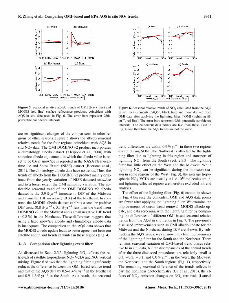
Figure 5. Seasonal relative albedo trends of OMI (black line) andMODIS (red line) surface reflectance products, coincident withAQS in situ data used in Fig. 6. The error bars represent 95th-percentile confidence intervals.

are no significant changes of the comparisons in other re-gions or other seasons. Figure 5 shows the albedo seasonalrelative trends for the four regions coincident with AQS insitu NO2 data. The OMI DOMINO v2 product incorporatesa climatology albedo dataset (Kleipool et al., 2008) withsnow/ice albedo adjustment, in which the albedo value is re-set to be 0.6 if snow/ice is reported in the NASA Near-real-time Ice and Snow Extent (NISE) dataset (Boersma et al.,2011). The climatology albedo data have no trends. Thus, thetrends of albedo from the DOMINO v2 product mainly orig-inate from the yearly variation of NISE-detected snow/iceand to a lesser extent the OMI sampling variation. The no-ticeable seasonal trend of the OMI DOMINO v2 albedodataset is the 3.9 % yr−1 increase in DJF of the Midwestand a smaller DJF increase (1.0 %) of the Northeast. In con-trast, the MODIS albedo dataset exhibits a smaller positiveDJF trend (0.8 % yr−1), 3.1 % yr−1 less than the trend fromDOMINO v2, in the Midwest and a small negative DJF trend(−0.8 %) in the Northeast. These differences suggest thatusing a fixed snow/ice albedo and climatology albedo datais inadequate. The comparison to the AQS data shows thatthe MODIS albedo update leads to better agreement betweensatellite and in suit trends in winter in these regions (Fig. 4).

3.1.3 Comparison after lightning event filter

As discussed in Sect. 2.3.3, lightning NOx affects the re-trievals of satellite tropospheric NO2 VCDs and NO2 verticalmixing. Figure 6 shows that the lightning filter significantlyreduces the difference between the OMI-based relative trendand that of the AQS data by 0.5–1.4 % yr−1 in the Northeastand 0.9–1.3 % yr−1 in the South. As a result, the seasonal

Figure 6. Seasonal relative trends of NO2 calculated from the AQSin situ measurements (“AQS”, black line) and those derived fromOMI data after applying the lightning filter (“OMI (lightning fil-ter)”, red line). The error bars represent 95th-percentile confidenceintervals. The coincident data points are less than those used inFig. 4, and therefore the AQS trends are not the same.

trend differences are within 0.9 % yr−1 in these two regionsexcept during SON. The Northeast is affected by the light-ning filter due to lightning in this region and transport oflightning NOx from the South (Sect. 2.3.3). The lightningfilter has little effect on the West and the Midwest. Whilelightning NOx can be significant during the monsoon sea-son in some regions of the West (Fig. 3), the average tropo-spheric NO2 VCDs are usually < 1× 1015 molecules cm−2,and lightning-affected regions are therefore excluded in trendanalysis.

The effect of the lightning filter (Fig. 6) cannot be shownin Fig. 4 because the coincident OMI and AQS data pointsare fewer after applying the lightning filter. We examine theimprovements of ocean trend removal, MODIS albedo up-date, and data screening with the lightning filter by compar-ing the differences of different OMI-based seasonal relativetrends from the AQS in situ trends in Fig. 7. The previouslydiscussed improvements such as OMI albedo update for theMidwest and the Northeast during DJF are shown. By sub-tracting the AQS trends, we can now find clear improvementsof the lightning filter for the South and the Northeast. Thereremains seasonal variation of OMI-based trend biases rela-tive to in situ data, but the discrepancies of the annual trendsafter the three discussed procedures are relatively small at0.3, −0.3, −0.1, and 0.0 % yr−1, in the West, the Midwest,the Northeast, and the South regions (Fig. 1), respectively.The remaining seasonal difference of the trends reflects inpart the nonlinear photochemistry (Gu et al., 2013), the ef-fects of NOx emission changes on NO2 retrievals (Lamsal

www.atmos-meas-tech.net/11/3955/2018/ Atmos. Meas. Tech., 11, 3955–3967, 2018

3962 R. Zhang et al.: Comparing OMI-based and EPA AQS in situ NO2 trends

Table 1. Annual relative trends calculated with coincident data and all available data. The 95th-percentile confidence intervals from Mann–Kendall method are also listed.

Region Annual relative trends of coincident data (% yr−1) Annual relative trends using all data (% yr−1)

Standard Lightning filtera Standard Lightning filter

AQS OMI AQS OMI AQS OMIb AQS OMIb

West −4.1± 0.5 −3.2± 0.4 −4.2± 0.5 −3.8± 0.4 −4.1± 0.5 −0.9± 0.4 −4.2± 0.5 −2.0± 0.3Midwest −3.4± 0.5 −3.6± 0.4 −2.8± 0.6 −3.1± 0.5 −2.5± 0.5 −0.9± 0.4 −2.2± 0.5 −1.8± 0.4Northeast −5.8± 0.5 −5.0± 0.5 −5.2± 0.6 −5.3± 0.7 −4.7± 0.5 −3.0± 0.4 −4.1± 0.5 −3.1± 0.5South −3.8± 0.4 −2.7± 0.3 −3.0± 0.5 −3.0± 0.5 −3.5± 0.4 −0.2± 0.4 −3.0± 0.5 −0.9± 0.3Nationwide −4.3± 0.4 −3.5± 0.3 −4.1± 0.4 −3.9± 0.3 −4.0± 0.4 −0.7± 0.3 −3.9± 0.4 −1.5± 0.2

a These data include the three data processing procedures of this study, namely, ocean trend correction, MODIS albedo update, and lightning filter screening. b Thespatial coverage is shown in Fig. 1.

Figure 7. Seasonal differences of OMI-based relative trends fromthose computed from AQS in situ data. The error bars represent95th-percentile confidence intervals. The relative trends are shownin Figs. 4 and 6. The figure legends are the same as in Figs. 4 and 6but with the AQS trends subtracted from the OMI-based trends.

et al., 2015), different spatial coverages of the two measure-ments, and the inherent difference between trends of NO2tropospheric VCDs and surface concentrations.

3.2 OMI-based NO2 trends

Table 1 summarizes the regional annual trends of coincidentAQS in situ and OMI data. The standard OMI data (followingthe DOMINO v2 algorithm) tend to show less NO2 reductionthan AQS data. After applying the three data processing pro-cedures discussed in the previous section to the OMI data,the agreement with the AQS trends is within the uncertain-ties of the trends. While lightning NOx is part of OMI NO2observations, we treat the influence of lightning on the OMItropospheric VCD trend as a bias for comparison purposes in

this study. Table 1 shows the effects of data sampling whenboth AQS and OMI data are analyzed and when the lightningfilter is applied.

Without the lightning filter, AQS decreasing trends arestronger than the decreasing trends of OMI data (Fig. 7). Thelightning trend in the NLDN data is unclear due in part tothe changing instrument sensitivity (Koshak et al., 2015). Iflightning NOx is not accounted for in OMI retrieval, tropo-spheric NO2 VCDs are overestimated. On the other hand,lightning accompanies low-pressure systems which mix theatmosphere vertically and tend to reduce surface NO2 con-centrations when anthropogenic emissions are high, such asurban and suburban regions. Therefore, lightning has oppo-site effects on surface and satellite trends. The low-pressuredilution effect on surface NO2 concentrations depends on an-thropogenic emissions (since the end point of dilution is thebackground NO2 value). Therefore, the weaker decreasingsurface trends likely reflect a reduction of the low-pressuredilution effect. Similarly, as anthropogenic emissions de-crease, the positive bias of tropospheric VCDs due to light-ning NOx becomes larger, likely resulting in weaker decreas-ing trends. We consider the lightning effects on surface NO2trends to be mostly meteorologically driven not by light-ning NOx directly (e.g., Ott et al., 2010; Luo et al., 2017),and hence the filtered OMI NO2 data are likely closer toemission-related concentration changes.

The AQS in situ NO2 annual relative trends (co-incident with OMI data with the lightning filter) aremost significant in the Northeast (−5.2± 0.6 % yr−1) andthe West (−4.2± 0.5 % yr−1), followed by the South(−3.0± 0.5 % yr−1) and the Midwest (−2.8± 0.6 % yr−1)regions. The nationwide annual trend is −4.1± 0.4 % yr−1,which is consistent with the previous studies (Lamsal etal., 2015; Lu et al., 2015; Tong et al., 2015; de Foy etal., 2016b; Duncan et al., 2016; Krotkov et al., 2016).The significant NO2 reductions result from updated tech-nologies and strict regulations (Krotkov et al., 2016).The OMI-based NO2 trends with the discussed proce-dures (coincident with AQS data) show similar reduc-

Atmos. Meas. Tech., 11, 3955–3967, 2018 www.atmos-meas-tech.net/11/3955/2018/

R. Zhang et al.: Comparing OMI-based and EPA AQS in situ NO2 trends 3963

Figure 8. Annual relative trends of OMI-based NO2 for “standard” (a) and for “lightning filter” (b) as the colored background. Black-bordered circles indicate corresponding AQS NO2 trends. Grid cells with 2005–2014 mean NO2 VCDs < 1× 1015 molecules cm−2 areexcluded in the analysis and are shown in white.

Figure 9. (a) The “lightning filter” OMI-based NO2 relative trend as a function 2005–2014-averaged OMI tropospheric NO2 VCD binnedevery 1× 1015 molec cm2. The error bars represent 95th-percentile confidence intervals. The red line shows a least-squares regression.(b) The distribution of 2005–2014-averaged OMI tropospheric NO2 VCD. Black-bordered circles represent AQS sites. The OMI troposphericNO2 data (“lightning filter”) are used.

tion rates in the West (−3.8± 0.4 % yr−1), the Midwest(−3.1± 0.5 % yr−1), the Northeast (−5.3± 0.7 % yr−1), andthe South (−3.0± 0.5 % yr−1) regions. The nationwide an-nual trend is −3.9± 0.3 % yr−1.

One advantage of satellite observations over a surfacemonitoring network is spatial coverage. The processed OMIdata (lightning filter) coincident with the AQS data show anational annual trend of −3.9± 0.3 % yr−1, similar to theAQS in situ trend of −4.1± 0.4 % yr−1. Using all data avail-able (Fig. 8, Table 1), the OMI data (lightning filter) showa much lower trend of −1.5± 0.2 % yr−1, about half of theAQS trend (−3.9± 0.4 % yr−1). Figure 9 shows that the AQSsites, which are mostly urban and suburban sites, tend tobe located in regions with high tropospheric NO2 VCDs.The OMI decreasing trend is a function of tropospheric NO2VCDs, increasing from 0 to−6 % yr−1 (Fig. 9). The nationalannual trend is close to the value of clean regions, whichcontribute much more than polluted regions. The larger de-crease near the anthropogenic source regions reflects in partthe nonlinear photochemistry (Gu et al., 2013) and in part a

stronger influence of NOx sources such as soils in rural re-gions.

4 Conclusions

Using data from the DOMINO v2 algorithm, we find thatthe computed OMI-based seasonal NO2 (relative) trends un-derestimate the decreasing trends of the EPA AQS data byup to 3.7 % yr−1. While lightning NOx is part of OMI NO2observations, we treat the influence of lightning on the OMItropospheric VCD trend as a bias for comparison purposesin this study. Furthermore, lightning NOx effects need to beremoved when using satellite observations to understand theeffects of changing anthropogenic emissions.

In this study, we show that removing the backgroundocean trend, adopting MODIS albedo data (with better tem-porospatial resolutions and characterization of snow/ice),and excluding lightning influences can bring OMI tro-pospheric NO2 VCD trends in close agreement (within

www.atmos-meas-tech.net/11/3955/2018/ Atmos. Meas. Tech., 11, 3955–3967, 2018

3964 R. Zhang et al.: Comparing OMI-based and EPA AQS in situ NO2 trends

0.3 % yr−1) with those of the AQS data. Among the correc-tions, the background ocean trend removal is not as signif-icant as the latter two. Since the origin of this trend is notyet clear, the ocean trend removal method may need up-dates in future studies. The remaining differences may resultfrom the inherent differences between trends of NO2 tro-pospheric VCDs and surface concentrations, different spa-tial sampling of the measurements, chemical nonlinearity,and tropospheric NO2 profile changes. The largest effectsof the MODIS albedo update are in winter in the Midwestand Northeast, and those of lightning filter are in the Southand the Northeast. After these data processing procedures areapplied, the derived OMI-based annual regional NO2 trendschange by a factor of > 2 for the South, the Midwest, andthe West, and seasonal changes can be even larger. We de-rive OMI-based NO2 regional annual relative trends using allavailable data for the West (−2.0 %± 0.3 yr−1), the Midwest(−1.8 %± 0.4 yr−1), the Northeast (−3.1 %± 0.5 yr−1), andthe South (−0.9 %± 0.3 yr−1).

The national annual trend of the processed OMIdata is −1.5± 0.2 % yr−1, about half of the AQS trend(−3.9± 0.4 % yr−1). It reflects that the AQS sites are mostlylocated in the urban and suburban regions, where OMI datashow much larger decreasing trends (up to −6 % yr−1) thanrural regions (down to 0 % yr−1). The reasons for the de-pendence of OMI-derived trends on tropospheric NO2 VCDsand the seasonal/regional trend differences are still not com-pletely understood. Further studies are necessary to improveour understanding of these trends. The observation-basedlightning filter implemented in this study is preliminary. In-corporating chemical transport modeling may improve thisfilter. Moreover, the results presented here represent an alter-native and indirect way to assess the importance of lightningNOx for National Climate Assessment (NCA) analyses de-scribed in Koshak et al. (2015) and Koshak (2017). Inversionstudies (e.g., Zhao and Wang, 2009; Gu et al., 2013, 2014,2016) will be needed to quantify the emission and AMFchanges corresponding to the OMI tropospheric NO2 VCDtrends.

Data availability. The datasets used in this research have been ob-tained online as follows:

– DOMINO v2 NO2 retrievals: http://www.temis.nl/airpollution/no2.html (last access: January 2016; Boersma et al., 2011).

– EPA AQS NO2 data: US Environmental Protection Agency.Air Quality System Data Mart (internet database) available at:http://www.epa.gov/ttn/airs/aqsdatamart (last access: January2016).

– NLDN lightning data: https://lightning.nsstc.nasa.gov/data/data_nldn.html (last access: January 2016; Cummins et al.,2016).

– MODIS MCD43B3 data: https://lpdaac.usgs.gov (LP DAAC,2016).

The Supplement related to this article is available onlineat https://doi.org/10.5194/amt-11-3955-2018-supplement.

Competing interests. The authors declare that they have no conflictof interest.

Acknowledgements. This work was supported by the NASA Atmo-spheric Composition Modeling and Analysis Program (ACMAP)and the NASA Climate Indicators and Data Products for FutureNational Climate Assessments (NNH14ZDA001N-INCA). Weacknowledge data sources, including DOMINO v2 OMI data fromKNMI, MODIS data from NASA, and EPA AQS NO2 data fromEPA. In addition, the authors gratefully acknowledge Vaisala Inc.for providing the NLDN data used in this study. K. Folkert Boersmaacknowledges funding from the EU FP7 project QA4ECV (grantno. 607405).

Edited by: Andreas RichterReviewed by: two anonymous referees

References

Bey, I., Jacob, D. J., Yantosca, R. M., Logan, J. A., Field,B. D., Fiore, A. M., Li, Q. B., Liu, H. G. Y., Mickley,L. J., and Schultz, M. G.: Global modeling of troposphericchemistry with assimilated meteorology: Model descriptionand evaluation, J. Geophys. Res.-Atmos., 106, 23073–23095,https://doi.org/10.1029/2001jd000807, 2001.

Boersma, K. F., Eskes, H. J., and Brinksma, E. J.: Error analysis fortropospheric NO2 retrieval from space, J. Geophys. Res.-Atmos.,109, D04311, https://doi.org/10.1029/2003JD003962, 2004.

Boersma, K. F., Eskes, H. J., Dirksen, R. J., van der A, R. J.,Veefkind, J. P., Stammes, P., Huijnen, V., Kleipool, Q. L., Sneep,M., Claas, J., Leitão, J., Richter, A., Zhou, Y., and Brunner, D.:An improved tropospheric NO2 column retrieval algorithm forthe Ozone Monitoring Instrument, Atmos. Meas. Tech., 4, 1905–1928, https://doi.org/10.5194/amt-4-1905-2011, 2011.

Bucsela, E. J., Pickering, K. E., Huntemann, T. L., Cohen, R. C.,Perring, A., Gleason, J. F., Blakeslee, R. J., Albrecht, R. I.,Holzworth, R., Cipriani, J. P., Vargas-Navarro, D., Mora-Segura,I., Pacheco-Hernández, A., and Laporte-Molina, S.: Lightning-generated NOx seen by the Ozone Monitoring Instrument dur-ing NASA’s Tropical Composition, Cloud and Climate Cou-pling Experiment (TC4), J. Geophys. Res.-Atmos., 115, D00J10,https://doi.org/10.1029/2009JD013118, 2010.

Castellanos, P. and Boersma, K. F.: Reductions in nitrogen oxidesover Europe driven by environmental policy and economic reces-sion, Sci. Rep., 2, 265, https://doi.org/10.1038/srep00265, 2012.

Cheng, Y., Wang, Y., Zhang, Y., Chen, G., Crawford, J.H., Kleb, M. M., Diskin, G. S., and Weinheimer, A. J.:Large biogenic contribution to boundary layer O3-CO regres-sion slope in summer, Geophys. Res. Lett., 44, 7061–7068,https://doi.org/10.1002/2017GL074405, 2017.

Atmos. Meas. Tech., 11, 3955–3967, 2018 www.atmos-meas-tech.net/11/3955/2018/

R. Zhang et al.: Comparing OMI-based and EPA AQS in situ NO2 trends 3965

Choi, Y., Wang, Y., Zeng, T., Martin, R. V., Kurosu, T. P.,and Chance, K.: Evidence of lightning NOx and con-vective transport of pollutants in satellite observationsover North America, Geophys. Res. Lett., 32, L02805,https://doi.org/10.1029/2004GL021436, 2005.

Choi, Y., Wang, Y., Zeng, T., Cunnold, D., Yang, E.-S., Martin,R., Chance, K., Thouret, V., and Edgerton, E.: Springtime tran-sitions of NO2, CO, and O3 over North America: Model eval-uation and analysis, J. Geophys. Res.-Atmos., 113, D20311,https://doi.org/10.1029/2007JD009632, 2008a.

Choi, Y., Wang, Y., Yang, Q., Cunnold, D., Zeng, T., Shim,C., Luo, M., Eldering, A., Bucsela, E., and Gleason, J.:Spring to summer northward migration of high O3 over thewestern North Atlantic, Geophys. Res. Lett., 35, L04818,https://doi.org/10.1029/2007GL032276, 2008b.

Cui, Y., Lin, J., Song, C., Liu, M., Yan, Y., Xu, Y., and Huang,B.: Rapid growth in nitrogen dioxide pollution over West-ern China, 2005–2013, Atmos. Chem. Phys., 16, 6207–6221,https://doi.org/10.5194/acp-16-6207-2016, 2016.

Cummins, K. L. and Murphy, M. J.: An Overview of Lightning Lo-cating Systems: History, Techniques, and Data Uses, With an In-Depth Look at the U.S. NLDN, IEEE T. Electromagn. C., 51,499–518, https://doi.org/10.1109/TEMC.2009.2023450, 2009.

Cummins, K. L., Burnett, R. O., Hiscox, W. L., and Pifer, A. E.:Line reliability and fault analysis using the National lightning de-tection network, Preprints, Precise Measurements in Power Con-ference, 27–29 October 1993, Arlington, VA, USA, 1993.

de Foy, B., Lu, Z., and Streets, D. G.: Satellite NO2 re-trievals suggest China has exceeded its NOx reductiongoals from the twelfth Five-Year Plan, Sci. Rep., 6, 35912,https://doi.org/10.1038/srep35912, 2016a.

de Foy, B., Lu, Z., and Streets, D. G.: Impacts of control strategies,the Great Recession and weekday variations on NO2 columnsabove North American cities, Atmos. Environ., 138, 74–86,https://doi.org/10.1016/j.atmosenv.2016.04.038, 2016b.

Demerjian, K. L.: A review of national monitoring net-works in North America, Atmos. Environ., 34, 1861–1884,https://doi.org/10.1016/S1352-2310(99)00452-5, 2000.

Dirksen, R. J., Boersma, K. F., Eskes, H. J., Ionov, D. V., Bucsela,E. J., Levelt, P. F., and Kelder, H. M.: Evaluation of stratosphericNO2 retrieved from the Ozone Monitoring Instrument: Intercom-parison, diurnal cycle, and trending, J. Geophys. Res.-Atmos.,116, D08305, https://doi.org/10.1029/2010JD014943, 2011.

Duncan, B. N., Yoshida, Y., de Foy, B., Lamsal, L. N., Streets,D. G., Lu, Z. F., Pickering, K. E., and Krotkov, N. A.: Theobserved response of Ozone Monitoring Instrument (OMI)NO2 columns to NOx emission controls on power plants inthe United States: 2005–2011, Atmos. Environ., 81, 102–111,https://doi.org/10.1016/j.atmosenv.2013.08.068, 2013.

Duncan, B. N., Lamsal, L. N., Thompson, A. M., Yoshida, Y., Lu,Z., Streets, D. G., Hurwitz, M. M., and Pickering, K. E.: Aspace-based, high-resolution view of notable changes in urbanNOx pollution around the world (2005–2014), J. Geophys. Res.-Atmos., 121, 976–996, https://doi.org/10.1002/2015JD024121,2016.

Eskes, H. J. and Boersma, K. F.: Averaging kernels for DOAS total-column satellite retrievals, Atmos. Chem. Phys., 3, 1285–1291,https://doi.org/10.5194/acp-3-1285-2003, 2003.

Gu, D., Wang, Y., Smeltzer, C., and Liu, Z.: Reductionin NOx Emission Trends over China: Regional and Sea-sonal Variations, Environ. Sci. Technol., 47, 12912–12919,https://doi.org/10.1021/es401727e, 2013.

Gu, D., Wang, Y., Smeltzer, C., and Boersma, K. F.: An-thropogenic emissions of NOx over China: Reconciling thedifference of inverse modeling results using GOME-2 andOMI measurements, J. Geophys. Res.-Atmos., 119, 7732–7740,https://doi.org/10.1002/2014JD021644, 2014.

Gu, D., Wang, Y., Yin, R., Zhang, Y., and Smeltzer, C.: Inverse mod-elling of NOx emissions over eastern China: uncertainties dueto chemical non-linearity, Atmos. Meas. Tech., 9, 5193–5201,https://doi.org/10.5194/amt-9-5193-2016, 2016.

Guenther, A. B., Jiang, X., Heald, C. L., Sakulyanontvittaya,T., Duhl, T., Emmons, L. K., and Wang, X.: The Model ofEmissions of Gases and Aerosols from Nature version 2.1(MEGAN2.1): an extended and updated framework for mod-eling biogenic emissions, Geosci. Model Dev., 5, 1471–1492,https://doi.org/10.5194/gmd-5-1471-2012, 2012.

Heckel, A., Kim, S.-W., Frost, G. J., Richter, A., Trainer, M., andBurrows, J. P.: Influence of low spatial resolution a priori dataon tropospheric NO2 satellite retrievals, Atmos. Meas. Tech., 4,1805–1820, https://doi.org/10.5194/amt-4-1805-2011, 2011.

Kain, J. S. and Fritsch, J. M.: Convective Parameterization forMesoscale Models: The Kain-Fritsch Scheme, in: The Repre-sentation of Cumulus Convection in Numerical Models, editedby: Emanuel, K. A., and Raymond, D. J., Am. Meteorol. Soc.,Boston, MA, USA, 165–170, 1993.

Kendall, M. G.: Rank correlation methods, Rank correlation meth-ods, Griffin, Oxford, UK, 1948.

Kleipool, Q. L., Dobber, M. R., de Haan, J. F., and Lev-elt, P. F.: Earth surface reflectance climatology from 3 yearsof OMI data, J. Geophys. Res.-Atmos., 113, D18308,https://doi.org/10.1029/2008JD010290, 2008.

Koshak, W. J.: Lightning NOx estimates from space-based light-ning imagers, 16th Annual Community Modeling and AnalysisSystem (CMAS) Conference, 23–25 October 2017, Chapel Hill,NC, USA, 2017.

Koshak, W. J., Cummins, K. L., Buechler, D. E., Vant-Hull, B.,Blakeslee, R. J., Williams, E. R., and Peterson, H. S.: Variabil-ity of CONUS Lightning in 2003–12 and Associated Impacts, J.Appl. Meteorol. Clim., 54, 15–41, https://doi.org/10.1175/jamc-d-14-0072.1, 2015.

Krotkov, N. A., McLinden, C. A., Li, C., Lamsal, L. N., Celarier,E. A., Marchenko, S. V., Swartz, W. H., Bucsela, E. J., Joiner,J., Duncan, B. N., Boersma, K. F., Veefkind, J. P., Levelt, P. F.,Fioletov, V. E., Dickerson, R. R., He, H., Lu, Z., and Streets,D. G.: Aura OMI observations of regional SO2 and NO2 pollu-tion changes from 2005 to 2015, Atmos. Chem. Phys., 16, 4605–4629, https://doi.org/10.5194/acp-16-4605-2016, 2016.

Lamsal, L. N., Martin, R. V., van Donkelaar, A., Steinbacher, M.,Celarier, E. A., Bucsela, E., Dunlea, E. J., and Pinto, J. P.:Ground-level nitrogen dioxide concentrations inferred from thesatellite-borne Ozone Monitoring Instrument, J. Geophys. Res.-Atmos., 113, D16308, https://doi.org/10.1029/2007JD009235,2008.

Lamsal, L. N., Martin, R. V., van Donkelaar, A., Celarier,E. A., Bucsela, E. J., Boersma, K. F., Dirksen, R., Luo,C., and Wang, Y.: Indirect validation of tropospheric nitro-

www.atmos-meas-tech.net/11/3955/2018/ Atmos. Meas. Tech., 11, 3955–3967, 2018

3966 R. Zhang et al.: Comparing OMI-based and EPA AQS in situ NO2 trends

gen dioxide retrieved from the OMI satellite instrument: In-sight into the seasonal variation of nitrogen oxides at north-ern midlatitudes, J. Geophys. Res.-Atmos., 115, D05302,https://doi.org/10.1029/2009JD013351, 2010.

Lamsal, L. N., Krotkov, N. A., Celarier, E. A., Swartz, W. H.,Pickering, K. E., Bucsela, E. J., Gleason, J. F., Martin, R. V.,Philip, S., Irie, H., Cede, A., Herman, J., Weinheimer, A., Szyk-man, J. J., and Knepp, T. N.: Evaluation of OMI operationalstandard NO2 column retrievals using in situ and surface-basedNO2 observations, Atmos. Chem. Phys., 14, 11587–11609,https://doi.org/10.5194/acp-14-11587-2014, 2014.

Lamsal, L. N., Duncan, B. N., Yoshida, Y., Krotkov, N.A., Pickering, K. E., Streets, D. G., and Lu, Z.: U.S.NO2 trends (2005–2013): EPA Air Quality System (AQS)data versus improved observations from the Ozone Mon-itoring Instrument (OMI), Atmos. Environ., 110, 130–143,https://doi.org/10.1016/j.atmosenv.2015.03.055, 2015.

Land Processes Distributed Active Archive Center (LP DAAC):MODIS/Terra+Aqua Albedo 16-Day L3 Global 1km SIN GridV004, Sioux Falls, South Dakota, USA, U.S. Geological Survey,V003, available at: https://lpdaac.usgs.gov, last access: January2016.

Laughner, J. L., Zare, A., and Cohen, R. C.: Effects ofdaily meteorology on the interpretation of space-based re-mote sensing of NO2, Atmos. Chem. Phys., 16, 15247–15264,https://doi.org/10.5194/acp-16-15247-2016, 2016.

Lin, J.-T. and McElroy, M. B.: Detection from space of a reductionin anthropogenic emissions of nitrogen oxides during the Chi-nese economic downturn, Atmos. Chem. Phys., 11, 8171–8188,https://doi.org/10.5194/acp-11-8171-2011, 2011.

Lin, J.-T., McElroy, M. B., and Boersma, K. F.: Constraint ofanthropogenic NOx emissions in China from different sec-tors: a new methodology using multiple satellite retrievals, At-mos. Chem. Phys., 10, 63–78, https://doi.org/10.5194/acp-10-63-2010, 2010.

Lin, J.-T., Liu, Z., Zhang, Q., Liu, H., Mao, J., and Zhuang,G.: Modeling uncertainties for tropospheric nitrogen dioxidecolumns affecting satellite-based inverse modeling of nitro-gen oxides emissions, Atmos. Chem. Phys., 12, 12255–12275,https://doi.org/10.5194/acp-12-12255-2012, 2012.

Lin, J.-T., Pan, D., and Zhang, R.: Trend and Interan-nual Variability of Chinese Air Pollution since 2000in Association with Socioeconomic Development: ABrief Overview, Atmos. Ocean. Sci. Lett., 6, 84–89,https://doi.org/10.1080/16742834.2013.11447061, 2013.

Lin, J.-T., Martin, R. V., Boersma, K. F., Sneep, M., Stammes,P., Spurr, R., Wang, P., Van Roozendael, M., Clémer, K., andIrie, H.: Retrieving tropospheric nitrogen dioxide from theOzone Monitoring Instrument: effects of aerosols, surface re-flectance anisotropy, and vertical profile of nitrogen dioxide, At-mos. Chem. Phys., 14, 1441–1461, https://doi.org/10.5194/acp-14-1441-2014, 2014.

Lin, J.-T., Liu, M.-Y., Xin, J.-Y., Boersma, K. F., Spurr, R., Martin,R., and Zhang, Q.: Influence of aerosols and surface reflectanceon satellite NO2 retrieval: seasonal and spatial characteristicsand implications for NOx emission constraints, Atmos. Chem.Phys., 15, 11217–11241, https://doi.org/10.5194/acp-15-11217-2015, 2015.

Liu, F., Beirle, S., Zhang, Q., van der A, R. J., Zheng, B., Tong,D., and He, K.: NOx emission trends over Chinese cities es-timated from OMI observations during 2005 to 2015, Atmos.Chem. Phys., 17, 9261–9275, https://doi.org/10.5194/acp-17-9261-2017, 2017.

Liu, Z., Wang, Y., Gu, D., Zhao, C., Huey, L. G., Stickel, R., Liao, J.,Shao, M., Zhu, T., Zeng, L., Liu, S.-C., Chang, C.-C., Amoroso,A., and Costabile, F.: Evidence of Reactive Aromatics As a Ma-jor Source of Peroxy Acetyl Nitrate over China, Environ. Sci.Technol., 44, 7017–7022, https://doi.org/10.1021/es1007966,2010.

Liu, Z., Wang, Y., Vrekoussis, M., Richter, A., Wittrock, F.,Burrows, J. P., Shao, M., Chang, C.-C., Liu, S.-C., Wang,H., and Chen, C.: Exploring the missing source of glyoxal(CHOCHO) over China, Geophys. Res. Lett., 39, L10812,https://doi.org/10.1029/2012GL051645, 2012a.

Liu, Z., Wang, Y., Gu, D., Zhao, C., Huey, L. G., Stickel, R.,Liao, J., Shao, M., Zhu, T., Zeng, L., Amoroso, A., Costabile,F., Chang, C.-C., and Liu, S.-C.: Summertime photochemistryduring CAREBeijing-2007: ROx budgets and O3 formation, At-mos. Chem. Phys., 12, 7737–7752, https://doi.org/10.5194/acp-12-7737-2012, 2012b.

Lu, Z., Streets, D. G., de Foy, B., Lamsal, L. N., Duncan, B.N., and Xing, J.: Emissions of nitrogen oxides from US ur-ban areas: estimation from Ozone Monitoring Instrument re-trievals for 2005–2014, Atmos. Chem. Phys., 15, 10367–10383,https://doi.org/10.5194/acp-15-10367-2015, 2015.

Luo, C., Wang, Y., and Koshak, W. J.: Development ofa self-consistent lightning NOx simulation in large-scale3-D models, J. Geophys. Res.-Atmos., 122, 3141–3154,https://doi.org/10.1002/2016JD026225, 2017.

Mann, H. B.: Nonparametric Tests Against Trend, Econometrica,13, 245–259, https://doi.org/10.2307/1907187, 1945.

Martin, R. V., Sauvage, B., Folkins, I., Sioris, C. E., Boone, C.,Bernath, P., and Ziemke, J.: Space-based constraints on the pro-duction of nitric oxide by lightning, J. Geophys. Res.-Atmos.,112, D09309, https://doi.org/10.1029/2006JD007831, 2007.

Ott, L. E., Pickering, K. E., Stenchikov, G. L., Allen, D. J., De-Caria, A. J., Ridley, B., Lin, R.-F., Lang, S., and Tao, W.-K.: Production of lightning NOx and its vertical distributioncalculated from three-dimensional cloud-scale chemical trans-port model simulations, J. Geophys. Res.-Atmos., 115, D04301,https://doi.org/10.1029/2009JD011880, 2010.

Pickering, K. E., Wang, Y., Tao, W.-K., Price, C., and Müller, J.-F.: Vertical distributions of lightning NOx for use in regional andglobal chemical transport models, J. Geophys. Res.-Atmos., 103,31203–31216, https://doi.org/10.1029/98JD02651, 1998.

Rudlosky, S. D. and Fuelberg, H. E.: Pre- and Postupgrade Distribu-tions of NLDN Reported Cloud-to-Ground Lightning Character-istics in the Contiguous United States, Mon. Weather Rev., 138,3623–3633, https://doi.org/10.1175/2010mwr3283.1, 2010.

Russell, A. R., Perring, A. E., Valin, L. C., Bucsela, E. J., Browne,E. C., Wooldridge, P. J., and Cohen, R. C.: A high spa-tial resolution retrieval of NO2 column densities from OMI:method and evaluation, Atmos. Chem. Phys., 11, 8543–8554,https://doi.org/10.5194/acp-11-8543-2011, 2011.

Russell, A. R., Valin, L. C., and Cohen, R. C.: Trends in OMINO2 observations over the United States: effects of emissioncontrol technology and the economic recession, Atmos. Chem.

Atmos. Meas. Tech., 11, 3955–3967, 2018 www.atmos-meas-tech.net/11/3955/2018/

R. Zhang et al.: Comparing OMI-based and EPA AQS in situ NO2 trends 3967

Phys., 12, 12197–12209, https://doi.org/10.5194/acp-12-12197-2012, 2012.

Saha, S., Moorthi, S., Pan, H.-L., Wu, X., Wang, J., Nadiga, S.,Tripp, P., Kistler, R., Woollen, J., Behringer, D., Liu, H., Stokes,D., Grumbine, R., Gayno, G., Wang, J., Hou, Y.-T., Chuang, H.-Y., Juang, H.-M. H., Sela, J., Iredell, M., Treadon, R., Kleist,D., Van Delst, P., Keyser, D., Derber, J., Ek, M., Meng, J., Wei,H., Yang, R., Lord, S., Van Den Dool, H., Kumar, A., Wang,W., Long, C., Chelliah, M., Xue, Y., Huang, B., Schemm, J.-K.,Ebisuzaki, W., Lin, R., Xie, P., Chen, M., Zhou, S., Higgins, W.,Zou, C.-Z., Liu, Q., Chen, Y., Han, Y., Cucurull, L., Reynolds, R.W., Rutledge, G., and Goldberg, M.: The NCEP Climate Fore-cast System Reanalysis, B. Am. Meteorol. Soc., 91, 1015–1057,https://doi.org/10.1175/2010BAMS3001.1, 2010.

Schaaf, C. B., Gao, F., Strahler, A. H., Lucht, W., Li, X., Tsang,T., Strugnell, N. C., Zhang, X., Jin, Y., Muller, J.-P., Lewis, P.,Barnsley, M., Hobson, P., Disney, M., Roberts, G., Dunderdale,M., Doll, C., d’Entremont, R. P., Hu, B., Liang, S., Privette, J. L.,and Roy, D.: First operational BRDF, albedo nadir reflectanceproducts from MODIS, Remote Sens. Environ., 83, 135–148,https://doi.org/10.1016/S0034-4257(02)00091-3, 2002.

Schenkeveld, V. M. E., Jaross, G., Marchenko, S., Haffner,D., Kleipool, Q. L., Rozemeijer, N. C., Veefkind, J. P.,and Levelt, P. F.: In-flight performance of the Ozone Mon-itoring Instrument, Atmos. Meas. Tech., 10, 1957–1986,https://doi.org/10.5194/amt-10-1957-2017, 2017.

Tang, J., Zhang, A., and He, Z.: The earth surface reflectance re-trieval by exploiting the synergy of TERRA and AQUA MODISdata, 2007 IEEE International Geoscience and Remote SensingSymposium, 23–28 July 2007, Barcelona, Spain, 1697–1700,https://doi.org/10.1109/IGARSS.2007.4423144, 2007.

Tong, D. Q., Lamsal, L., Pan, L., Ding, C., Kim, H., Lee, P.,Chai, T., Pickering, K. E., and Stajner, I.: Long-term NOx

trends over large cities in the United States during the greatrecession: Comparison of satellite retrievals, ground observa-tions, and emission inventories, Atmos. Environ., 107, 70–84,https://doi.org/10.1016/j.atmosenv.2015.01.035, 2015.

Yang, Q., Wang, Y., Zhao, C., Liu, Z., Gustafson, W. I., and Shao,M.: NOx Emission Reduction and its Effects on Ozone duringthe 2008 Olympic Games, Environ. Sci. Technol., 45, 6404–6410, https://doi.org/10.1021/es200675v, 2011.

Zara, M., Boersma, K. F., De Smedt, I., Richter, A., Peters, E., VanGeffen, J. H. G. M., Beirle, S., Wagner, T., Van Roozendael, M.,Marchenko, S., Lamsal, L. N., and Eskes, H. J.: Improved slantcolumn density retrieval of nitrogen dioxide and formaldehydefor OMI and GOME-2A from QA4ECV: intercomparison, un-certainty characterization, and trends, Atmos. Meas. Tech. Dis-cuss., https://doi.org/10.5194/amt-2017-453, in review, 2018.

Zhang, R., Wang, Y., He, Q., Chen, L., Zhang, Y., Qu, H., Smeltzer,C., Li, J., Alvarado, L. M. A., Vrekoussis, M., Richter, A., Wit-trock, F., and Burrows, J. P.: Enhanced trans-Himalaya pollu-tion transport to the Tibetan Plateau by cut-off low systems, At-mos. Chem. Phys., 17, 3083–3095, https://doi.org/10.5194/acp-17-3083-2017, 2017.

Zhang, Y. and Wang, Y.: Climate-driven ground-level ozone extreme in the fall over the SoutheastUnited States, P. Natl. Acad. Sci., 113, 10025-10030,https://doi.org/10.1073/pnas.1602563113, 2016.

Zhang, Y., Wang, Y., Chen, G., Smeltzer, C., Crawford, J.,Olson, J., Szykman, J., Weinheimer, A. J., Knapp, D. J.,Montzka, D. D., Wisthaler, A., Mikoviny, T., Fried, A., andDiskin, G.: Large vertical gradient of reactive nitrogen oxidesin the boundary layer: Modeling analysis of DISCOVER-AQ2011 observations, J. Geophys. Res.-Atmos., 121, 1922–1934,https://doi.org/10.1002/2015JD024203, 2016.

Zhao, C. and Wang, Y.: Assimilated inversion of NOx emissionsover east Asia using OMI NO2 column measurements, Geophys.Res. Lett., 36, L06805, https://doi.org/10.1029/2008GL037123,2009.

Zhao, C., Wang, Y., Choi, Y., and Zeng, T.: Summertime impact ofconvective transport and lightning NOx production over NorthAmerica: modeling dependence on meteorological simulations,Atmos. Chem. Phys., 9, 4315–4327, https://doi.org/10.5194/acp-9-4315-2009, 2009.

Zhou, Y., Brunner, D., Boersma, K. F., Dirksen, R., and Wang, P.:An improved tropospheric NO2 retrieval for OMI observationsin the vicinity of mountainous terrain, Atmos. Meas. Tech., 2,401–416, https://doi.org/10.5194/amt-2-401-2009, 2009.

www.atmos-meas-tech.net/11/3955/2018/ Atmos. Meas. Tech., 11, 3955–3967, 2018