COMPARING EARLY WARNING SYSTEMS FOR …ephilipdavis.com/earlywarning.pdfCOMPARING EARLY WARNING...

COMPARING EARLY WARNING SYSTEMS

FOR BANKING CRISES

E Philip Davis and Dilruba Karim1 Brunel University and NIESR

West London Abstract: Despite the extensive literature on prediction of banking crises by Early Warning Systems (EWS), their practical use by policy makers is limited, even in the international financial institutions. This is a paradox since the changing nature of banking risks as more economies liberalise and develop their financial systems, as well as ongoing innovation, makes the use of EWS for crisis prevention more necessary than ever. In this context, we assess the logit and signal extraction EWS for banking crises on a comprehensive common dataset. We suggest that logit is the most appropriate approach for global EWS and signal extraction for country specific EWS. Furthermore it is important to consider the policy maker�s objectives when designing predictive models and setting related thresholds since there is a sharp trade-off between correctly calling crises and false alarms. Keywords: Banking crises, systemic risk, early warning systems, logit estimation, signal extraction JEL Classification: C52, E58, G21

1 Davis is Professor of Economics and Finance and Karim is a Doctoral Research Student, Department of Economics and Finance, School of Social Sciences, Brunel University, Uxbridge, Middlesex, UB8 3PH, UK, emails [email protected] and [email protected]. Davis is also Visiting Fellow, NIESR, Dean Trench Street, Smith Square, London SW1.

2

Introduction

Historic episodes of financial crises highlight the need for Early Warning Systems (EWS) for

banking crisis prediction; over 1980-1996, three-quarters of IMF countries experienced

banking distress (Lindgren, Garcia and Saal, 1996). Crises were not restricted to particular

geographic regions, levels of development or banking system structures2. A working

definition of a banking crisis is the �occurrence of severely impaired ability of banks to

perform their intermediary role�. Restriction to a few banks constitutes a localised crisis

whereas collapse of the banking system constitutes a systemic crisis.

Systemic crises have significant direct and indirect costs. According to Caprio and Klingebiel

(1996), bailout costs average 10% of GDP, with some crises much more costly, e.g. the

Mexican Tequila Crisis (1994) cost 20% of GDP whilst the Jamaican crisis (1996) cost 37%

of GDP. There are additional costs of foregone economic output (notably reduced investment

and consumption) owing inter alia to credit rationing and uncertainty. Hoggarth and Sapporta

(2001) estimate that cumulative output losses from banking and twin crises3 were much

greater in OECD countries (23.8% of GDP) than in emerging market economies (13.9%).

Banking crises alone cost an average of 5.6% of GDP and twin crises 29.9%.

The IMF uses an early warning system (EWS) to monitor currency crises but has no explicit

EWS for banking crises. Likewise, private sector institutions focus on currency crisis

prediction. This may partly reflect the historically high prevalence of currency crises; in a

study of 20 countries, Kaminsky and Reinhart (1999) found that during the 1970s there were

26 currency crises and only 3 banking crises (due to financial repression). However, banking

crises quadrupled in the post-liberalisation period of the 1980s and 1990s. Further increases

are foreseeable as additional emerging market countries undergo financial liberalisation, while

in more advanced economies, securitised financial markets develop new financially

engineered products whose behaviour during recessions is not well understood. For example,

Chan et al (2006) note the close relationship between banks and hedge funds which undertake

unregulated investments. Related risks are not well understood, but as the LTCM crisis in

2 Caprio and Klingebiel (1996). 3 Defined as cases where a currency crisis occurs within the period 2 years before and after the banking crisis. Whereas one might anticipate that a currency crisis would mitigate the impact of the banking crisis by increasing the profitability of export and import-competing firms, it seems that this is more than offset by a greater level of financial disruption in a twin crisis, in many cases including a cut-off of international credit, that may aggravate the banking crisis (Kaminsky and Reinhart 1999).

3

1998 demonstrated4, hedge funds with highly leveraged positions can rapidly magnify

domestic and international systemic risks, thereby increasing chances of contagion. Hence the

need to devise a reliable EWS for banking crisis prevention remains more pressing than ever.

Although models have been developed to allow banking crisis prediction, their comparative

performance is difficult to evaluate. Current models have been derived from various historic

datasets and more importantly, by using different dependent variables and overall

methodologies. Consequently, leading indicators may appear inconsistent and in-sample and

out-of-sample results differ. This paper attempts to resolve some of the current ambiguity on

predictive efficiency and indicator robustness. Our contribution includes the following: We

test two of the main EWS in the literature (multivariate logit and signal extraction) using a

single panel dataset. The cross-country and time-series coverage is more extensive than most

previous studies. We also consider refinements to current EWS by considering how banking

crisis theory could help to improve specification and variable choice. In the specific case of

signal extraction work we also distinguish country specific from general effects and construct

composite indicators.

In sum, our results show (1) that given the same underlying data, the choice of EWS does

make a difference to predictive efficiency. (2) Given the EWS model, the choice of dependent

variable determines predictive capacity. (3) Transforming indicators including

standardisation, lags and interaction terms improves the performance of the EWS. (4) Some

models are better for developing country-specific EWS whilst others are suited to global

EWS. (5) Combining variables into composite indicators improves crisis predictive ability.

The remainder of the article proceeds as follows: Section I provides a brief theoretical review

of banking crises which motivates the choice of indicators. Section II explains the

methodology we adopt, including the theory behind the logit and signal extraction methods,

construction of the banking crisis dependent variable and our dataset. Section III presents our

results, whilst section IV concludes.

1 Theoretical overview of banking crises.

This section briefly indicates why the indicators used in EWS models such as Demirguc-Kunt

and Detragiache (1998) (who use the logit method) are associated with banking crises.5 This

enables us to assess the variables� validity and also to recommend extensions.

4 Davis (1999)

4

Generally, banking systemic risk reflects a correlation of performance between institutions.

One possibility is that such crises can be purely self fulfilling, i.e. they materialise through

individual liquidity failures of solvent banks that become contagious. In these cases, crises

can be driven by asymmetric information and associated bank runs. Diamond and Dybvig

(1983) emphasised the role of confidence in precipitating runs and that arbitrary shifts in

investors� risk expectations explain seemingly irrational behaviour of consumers running on

banks; a bank�s underlying financial position is almost irrelevant once panic ensues. Hence

individual bank failure may spread through contagion associated with asymmetric information

and in this context systemic banking crises are self-fulfilling. This view has been criticised on

the view that there is usually a fundamental explanation for such events.

George (1998) suggests that systemic risks arise �through the direct financial exposures6

which tie firms together�. If systemic risk is sufficiently deep, (i.e. if correlations between

individual bank risks are particularly high), then crises could be triggered. Hence a further

possibility is that there could be counterparty claims between banks (e.g. via interbank

exposures) that lead to widespread failures.

EWS to date have typically ignored the possibility of pure self-fulfilling crises and crises

caused simply by counterparty exposures. This can be justified because historically the vast

majority of banking crises have been caused by financial institutions underestimating their

common exposure to economy wide systematic risk (Borio, Furfine and Lowe, 2001). This

may link to asymmetric information as if one significant bank fails, a systemic crisis may

develop because the presence of such asymmetric information means depositors are unable to

evaluate prospects for �similar� banks in terms of balance-sheet exposure to economy wide

systemic risks (Kaufman and Scott, 2003).

Accordingly, macroeconomic movements that crystallise risks particular to banking systems,

namely interest rate, credit, liquidity and market risk have been the key determinants of

banking crises in the last twenty years (Ergungor and Thompson, 2005). Correspondingly, in

most EWS studies, the explanatory variables used mainly capture macroeconomic factors that

could generate systemic risk via such common shocks.

5 We note that Kaminsky and Reinhart (1999) (who use the signal extraction method) use a different set of variables more closely associated with currency crisis prediction. 6 Exposures include inter-bank transactions, counterparty risk, or third party (non-bank institutional) failure.

5

Interest rate risk forms an inherent part of banking activities since assets have longer duration

than liabilities. Term structure shifts towards short-term liabilities (inverted yield curves)

adversely affect bank balance sheets by eroding bank spreads. Simultaneously, banks may

suffer prepayment risk if long-term rates decline and borrowers refinance at lower rates.

These outcomes adversely affect bank balance sheets and if there is significant exposure to

interest rate risk, net worth of the banking system becomes vulnerable.

Oviedo (2004) highlights the counter-cyclicality of interest rates; lower interest rates are

associated with economic booms when crises are less likely. Consequently, during booms,

banks may use low-cost deposit financing to invest heavily in particular sectors which appear

profitable and where collateral values are high. This increased appetite for long-term projects

means duration mismatch and interest rate risk are likely to accumulate during the boom

phase so that unexpected interest rate increases or moves towards inflation targeting in the

downturn could lead systemic interest rate risk to materialise. Hence the inclusion of real

interest rates in EWS and the observed, positive correlation between real interest rates and

banking crisis probability in recent work (Demirguc-Kunt and Detragiache, 1998; Hardy and

Pazarbasioglu, 1998; Kaminsky and Reinhart, 1999; Gourinchas, Valdes and Landerretche,

2001).

Another symptom of banking crises is increased credit risk or the probability that a borrower

will default, converting an asset into a �bad� or non-performing loan (NPL). Although banks

enjoy advantages in screening and monitoring borrowers, both of which reduce credit risk, the

high levels of NPLs associated with crises indicate risk assessment by banks deteriorates

during pre-crisis periods.

One reason for and consequence of inadequate credit risk evaluation is the procyclical

movement of lending and asset prices which allows for interaction of financial cycles and

business cycles. Periods of high output growth raise collateral values and as a result, during

booms loan contracts become less informationally dependent. Asymmetric information does

not restrict credit availability because bank managers succumb to �euphoric� and �herding�

behaviour7, utilising biased information sets to make investment decisions. As a result, they

ignore the potentially high default probabilities that could occur under recessionary states and

under-price credit risk. Borio, Furfine and Lowe (2001) attribute these sub-optimal

behavioural responses to difficulties in measuring time series of credit risk and to incentive

7 Davis (1995).

6

based managerial contracts which reward loan volume. As lending increases, this further

inflates asset prices, which raises collateral values and perpetuates the endogenous cycle

(Davis and Zhu 2004). The boom phase ends when shocks, such as asset price collapses, turn

the process backwards; during recessions managers may overestimate risk so that cyclical

downturns reverse the financial accelerator. As assets markets collapse, collateral values

decline and NPLs rise. Because asymmetric information becomes disproportionately

important for loan officers, lending spreads are artificially high and intermediaries hold excess

capital and provisions. Ultimately, credit rationing prevents borrowers with profitable projects

from obtaining funds and the recession deepens.

Credit risk may be particularly high and correlated between institutions when herding focuses

boom-phase investment to specific sectors of the economy. Over-investment in real estate

(particularly commercial) has been a well-documented feature of banking crises8 because the

value of bank capital increases if real estate forms the asset base. Bank lending therefore

magnifies the real estate cycle, leading to further financial acceleration and financial

instability (Herring and Wachter, 1998; Borio, Furfine and Lowe, 2001, Davis and Zhu 2004,

2005). Furthermore credit risk may be magnified by regulation that limits diversification.9

In the context of banking crises, market risk is intertwined with credit risk. Market risk

reflects the probability that price-volatility of specific assets affects the net worth of banks.

Such adverse price movements may arise through shifts in market expectations in anticipation

of cyclical downturns. Alternatively, specific asset groups may be hit by idiosyncratic factors,

e.g. oil price volatility following political events. Although market risk is diversifiable,

regulation limiting types of assets held may impede this. Alternatively, excessive market risk

may be borne during boom phases, as over-optimism may concentrate portfolios in assets

whose prices move procyclically, e.g. real estate (Gonzalez-Hermosillo, 1999, Craig et al

2005). Since credit risk is also procyclical, the link between the two risks becomes apparent

when asset price collapses realise market risk and low collateral values realise credit risk.

Banks may also be exposed to market risk if their portfolios are concentrated on equities and

currencies; if they fail to adequately provision against price volatility, then adverse price

shocks can jeopardise the net worth of the banking system.

8 See FDIC (1997) for the relationship between commercial real estate and US banking crises during the 1980s and 1990s. 9 The Texan Banking crisis was driven by regulation which forced regional banks and S&Ls to invest within their state. Texan institutions over-invested in the Texan oil industry which entered recession in 1987 (FDIC, 1997).

7

Banking liquidity risk reflects the probability that banks will be unable to satisfy the claims of

depositors because the ratio of illiquid assets relative to liquid liabilities is too high. In the

Diamond and Dybvig (1983) model, liquidity risk drives idiosyncratic bank runs. Liquidity

risk also links to adverse information models of banking crises (Santos, 2000). Chari and

Jagannathan (1988) modify the Diamond and Dybvig model to show that when depositors

assimilate adverse information (e.g. signals of recession or asset market collapses) they

anticipate that bank profitability will suffer. Resulting bank runs generate systemic liquidity

problems. These runs are distinct from the Diamond and Dybvig model where runs on solvent

banks occur even when depositors have no legitimate evidence to suspect insolvency. Rather,

in this case, depositors are more likely to run on genuinely insolvent banks. Hence Gorton�s

(1988) observation that panics are associated with recessions and Jacklin and Bhattacharya�s

(1988) suggestion that the release of information indicating low asset values or poor

performance of a bank can generate liquidity risk.

Financial liberalisation provides another source of the systemic risks mentioned, hence the

well-documented association between liberalisation and crises; in the Kaminsky and Reinhart

(1999) sample, over 70% of banking crises were preceded by financial liberalisation within

the last five years and the probability of banking crisis conditional on financial liberalisation

having occurred is higher than the unconditional probability of banking crisis. Demirguc-Kunt

and Detragiache (1998) also find financial liberalisation increases crisis risk within a few

years of the liberalisation process.

High real interest rates and increased interest rate volatility are typical consequences of

financial liberalisation, especially in developing countries (Honohan, 2000). During financial

repression, imposed ceilings mean real interest rates cannot adjust to clear credit markets and

credit rationing results in �non-market�, usually state-directed, credit allocation. Although

interest rate risk considerations are likely to be subordinate when states allocate credit,

interest rate ceilings have some risk limiting effect. However in post-liberalised environments,

wider spreads and increased competition could cause an accumulation of systemic interest

rate risk which may be more likely to materialise because of higher interest rate volatility.

Another effect of financial liberalisation may be to increase credit risk. In liberalised markets,

increased competition may erode bank charter values so that without adequate supervision

and regulation, banks forgo prudent credit risk assessment in a bid to catch borrowers. Hence

financial liberalisation can exaggerate procyclicality of asset prices by fuelling a consumption

8

boom (Borio, Furfine and Lowe (2002)). Craig et al (2005) suggest that credit risk increases

following liberalisation because the rapid increases in loan volumes constrain credit risk

assessment. This may be exacerbated in the presence of government safety nets; Demirguc-

Kunt and Detragiache (1998) show deposit insurance is a significant leading indicator of

banking crisis and the same authors (2002) show explicit deposit insurance increases the risk

of moral hazard when institutions are weak. Where financial liberalisation does increase asset

price volatility, there may also be increased liquidity risk borne by the system since banks are

unable to sell assets at par when asset prices collapse.

Looking at the indicators typically used in EWS models, in the light of the discussion above,

we would thus expect rapid real credit growth and increases in private sector credit/ GDP10

during pre-crisis periods, indicating credit risk accumulation. Similarly procyclicality of

financial instability implies GDP growth should capture boom and bust cycles. Liquidity risk

is incorporated by bank cash plus reserves as a proportion of total bank assets; the lower this

ratio the higher the systemic liquidity risk. Macroeconomic shocks which could trigger

cyclical downturns thereby increasing NPLs include adverse movements in terms of trade and

correspondingly currency depreciations, especially for small open economies. The latter also

indicates vulnerability to currency crisis, as does M2/ foreign exchange reserves since lower

ratios imply impaired ability to defend the currency. Real interest rates are used as a direct

indicator of interest rate risk. High inflation signals policy mismanagement which causes

higher nominal interest rates at the expense of lenders. Corresponding increases in interest

rate volatility should also capture interest rate risk. Higher inflation may also, to a certain

extent, reflect market risk of asset price booms. Direct use of asset prices such as real estate

for proxying market risk in EWS models has been limited due to lack of data outside the

OECD countries. On the other hand exchange rate based market risk is proxied by the terms

of trade and currency depreciations.

Policy mismanagement is also reflected in low fiscal surpluses/ GDP. Demirguc-Kunt and

Detragiache (1998) include this variable because it indicates governments� reluctance to

restructure fragile banking systems and because high deficits prevent successful financial

liberalisation. Real interest rates also act as a proxy for financial liberalisation. Furthermore,

Demirguc-Kunt and Detragiache rely on the level of GDP per capita as a structural economic

development measure which should be positively related to the quality of banking

10 However, the level of the credit/GDP ratio is rather an indicator of economic and financial development.

9

regulation11. Given these leading indicators, we now turn to describe the construction of the

banking crisis dependent variable and the actual models used to predict banking crises.

2 Data, variables and specifications

2.1 The Banking Crisis Variable

The most commonly-cited problem with EWS developed to date is the inconsistency in the

banking crisis dependent variable, which is necessarily defined with a degree of subjectivity

(Kaminsky and Reinhart, 1999; Demirguc-Kunt and Detragiache 1998, Eichengreen and

Arteta, 2000). There is no unique quantitative variable for banking crisis. The problem lies in

the fact that banking crisis is an event, so proxies for banking crises would not necessarily be

perfectly correlated with banking crises themselves. For instance, if we were to use a measure

for banking insolvency such as aggregate banking capital, we would need to define a lower

bound threshold for a crisis event. However, government intervention or deposit insurance

could prevent crisis and the threshold could still be violated. Another issue is that not all

crises stem from the liabilities side (Kaminsky and Reinhart, 1999); problems in asset quality

can also erode banking capital so that a single proxy variable would not pick up all crisis

events. As a result the dummy is constructed on the basis of several criteria which vary

according to the study. The main classifications are to be found in Caprio and Klingebiel

(1996, 2003), Demirguc-Kunt and Detragiache (1998, 2005), Kaminsky and Reinhart (1999)

and Lindgren, Garcia and Saal (1996).

Caprio and Klingebiel (1996) focus on the solvency side of crisis and define systemic crisis as

an event when �all or most of banking capital is exhausted�12. Insolvency was judged on the

basis of official data and published reports by financial market experts; if official data

recorded positive banking system capital but experts judged it to be negative, they recorded

systemic crisis13. Caprio and Klingebiel (2003) subsequently updated their database to the

period 1980-2002 and identified 93 countries as having experienced systemic crises.

11 Demirguc-Kunt and Detragiache (1998) also incorporate two other institutional variables: a deposit insurance dummy (where explicit deposit insurance means the dummy value is 1) and a law and order dummy. 12 They stipulate that non-performing loans as a proportion of entire loans of the banking system must be in the range of 5�10% or less. 13 On this criterion, they judged 58 countries to have experienced systemic crisis over the post-1970s period with many experiencing repeated episodes.

10

Demirguc-Kunt and Detragiache (1998) used a more specific set of four criteria14 where

achievement of at least one of the conditions was a requirement for systemic crisis, otherwise

bank failure was non-systemic. The authors admitted they relied on judgement if there was

insufficient evidence to support their crisis criteria; on this basis they established 31 systemic

crises in 65 countries over the 1980-1994 period. Demirguc-Kunt and Detragiache (2005)

conducted a follow up study and extended the sample to 1980-2002. Using the same criteria

as before, they find 77 systemic crises over 94 countries.

Kaminsky and Reinhart (1999) and Lindgren, Garcia and Saal (1996) use criteria similar15 to

Demirguc-Kunt and Detragiache (1998). Kaminsky and Reinhart (1999) identified 26

systemic banking crises over 20 countries during the period 1970-1995. Of the 26 crises, 19

are twinned with currency crises and the remaining 7 are pure banking crises.

Even if systemic crises unambiguously occur, identifying their starting and ending dates is

hazardous and the same episode may have a different duration in different studies. Where runs

do not occur and banking system data are either unavailable or unreliable, locating the exact

time when the system became insolvent is impossible. Even if runs do occur, this may be a

culmination of a prolonged period of systemic insolvency, which was either unknown to

depositors or supported by government assistance at and earlier stage. Based on the run, the

start date would �time� the crisis too late.

Kaminsky and Reinhart (1999) note that crises can also be dated too early, since the worst of

the crisis could unfold after the subjective start date. Dating is also problematic when there

are successions of crises episodes; in many such instances it is arguable that later crises are

extensions or re-emergences of previous financial distress as opposed to distinct crises events

(Caprio and Klingebiel, 1996). Judgment is also required to distinguish between periods of

systemic and non-systemic crisis; a degree of banking system insolvency must be decided

upon whereby failure of a few banks is recorded as a localised crisis and beyond this crisis

becomes systemic. Not all studies make this distinction in the same way so that a crisis may

14 The proportion of non-performing loans to total banking system assets exceeded 10%, or the public bailout cost exceeded 2% of GDP, or systemic crisis caused large scale bank nationalisation, or extensive bank runs were visible and if not, emergency government intervention was visible. 15 For Kaminsky and Reinhart (1999), a crisis is systemic if banks runs result in closure or nationalisation of at least one bank, or if there are no runs, large-scale government intervention, merging or nationalisation of one bank marks the beginning of the same for other banks. Lindgren, Garcia and Saal (1996) classify systemic crises on the basis of whether bank runs, portfolio shifts, bank collapses or large-scale government intervention occur. Any other episodes of financial instability are classed as non-systemic crises.

11

be a systemic event in one paper but remain excluded from the banking crisis dummy in

another.

Whichever crisis definition is used, the crisis duration must be handled carefully in order to

avoid endogeneity; once a crisis occurs it is likely to deepen any recession and affect the

explanatory variables. Studies have addressed this feedback in various ways: Demirguc-Kunt

and Detragiache (1998) conduct two sets of regressions, one by discarding all observations

after a crisis begins and another by discarding observations after a crisis has ended16. Others

have arbitrarily assumed a common duration for all crises, e.g. 18 months (Kaminsky and

Reinhart, 1999) or 1 year (Eichengreen and Arteta, 2000; Glick and Hutchinson, 1999).

The subjectivity associated with banking crisis identification may explain why almost all

authors have relied on the studies mentioned above, either wholly or in combination, to

construct their banking crisis variable. The disadvantage of this is that all research has focused

on a few assessments of crisis occurrence. The advantage is that it reduces multiplicity in the

dependent variable amongst studies. In this vein, we will also rely on the Demirguc-Kunt and

Detragiache (2005) and Caprio and Klingebiel (2003) crises lists. Henceforth we refer to the

Demirguc-Kunt and Detragiache (2005) dates/ dummy as DD05 and the Caprio and

Klingebiel (2003) dates/ dummy as CK03.

2.2 The Data Sample

The dataset of independent variables mimics the Demirguc-Kunt and Detragiache (1998)

approach, utilising most of their variables but for a wider selection of countries and for a

longer time span. We have used the same data source they cite: IFS and World Bank

Development Indicators to obtain annual data; full data sources are obtainable in Demirguc-

Kunt and Detragiache (1998). A maximum of 105 countries are included whilst the data spans

the period 1979 to 2003. Under the DD05 dating this yields 72 systemic crisis episodes; under

the less stringent CK03 definitions this yields 102 systemic crisis episodes. Almost half the

countries included in our full sample experienced no systemic crisis based on DD05 dates,

whereas under a fifth were non-crisis countries based on the CK03 dates.

As explained in Part 1, the explanatory variables chosen are macroeconomic, financial and

financial liberalisation indicators of crisis. Table 1 below gives the indicator list.

16 They find the results do not change significantly either way.

12

Table 1: The Demirguc-Kunt and Detragiache (1998) Variables

1. Real GDP Growth (%) 2. Change in Terms of Trade (%) 3. Nominal Depreciation (%) 4. Real Interest Rate (%) 5. Inflation (%)

Macroeconomic Variables

6. Fiscal Surplus/ GDP (%) 7. M2/ Foreign Exchange Reserves (%) 8. Credit to Private Sector/ GDP (%) 9. Bank Liquid Reserves/ Total Bank Assets (%) Financial Variables

10. Real Domestic Credit Growth (%) 11. Real GDP per Capita Institutional Variables 12. Deposit Insurance (binary dummy)

2.3 The Demirguc-Kunt and Detragiache (1998) Mulivariate Logit Model

The multivariate logit approach allowed Demirguc-Kunt and Detragiache (1998) to relate the

likelihood of occurrence or non-occurrence of a banking crisis to a vector of n explanatory

variables. The probability that the banking dummy takes a value of one (crisis occurs) at a

point in time is given by the value of the logistic cumulative distribution evaluated for the

data and parameters at that point in time. Thus,

( ) ( )it

itX'

X'

itit e1eXF1YobPr β

ββ

+=== (1)

where Yit is the banking crisis dummy for country i at time t, β is the vector of coefficients,

Xit is the vector of explanatory variables and F(β Xit) is the cumulative logistic distribution.

The parameters are obtained by maximum likelihood estimation where each possible value of

Yit contributes to the joint likelihood function so that the log likelihood becomes

( )( ) ( ) ( )( )[ ]∑∑= =

−−+=n

i

T

titeititeite XFYXFYLLog

1 1'1log1'log ββ (2)

The parameters obtained by maximising this function are not constant marginal effects of Xi

on the crisis probability since the underlying relationship is non-linear. Rather, the marginal

effect of Xit on Yit is given by the probability of crisis times the probability of no crisis times

13

the coefficient βi17. Since the probabilities depend on the values of Xit, for a given coefficient,

a single explanatory variable can have changing marginal contributions to crisis probability

depending on its starting level. The sigmoidal logistic cumulative distribution shows that an

explanatory variable will make marginally little difference to crisis if the crisis probability is

already at the extreme (low or high) but if crisis probability is around the 0.5 range then a

change in the same variable is more likely to tip the balance and trigger crisis18. The sign on

the coefficient still indicates the direction of change on crisis probability. To directly compare

the individual contributions of each variable to crisis, their marginal effects can be computed

for their mean values (Greene, 2000) or at a specific year before a crisis unfolds.

Demirguc-Kunt and Detragiache (1998) do not use a fixed effects logit model; a fixed effects

model would mean the country specific dummy and the banking crisis dummy would be

perfectly correlated for countries which never experienced a banking crisis. Excluding these

countries would generate a biased sample and biased coefficients. Rather, they use a sample

composed of crisis and non-crisis countries where the latter represent controls. In this way,

variation in the explanatory variables is fully used to explain why crisis will or will not occur.

The advantage of this parametric approach is that it takes into account the interdependencies

of explanatory variables which in combination could trigger crisis. In this sense, the model

corresponds to much of the theory outlined in Part 1 where concurrent increases in real

interest rates, GDP and credit growth in the presence of financial liberalisation seem to

predispose economies to crisis.

2.4 The Kaminsky and Reinhart (1999) Signal Extraction Model

This is a non-parametric approach which assesses the behaviour of single variables prior to

and during crisis episodes. The logic is that if aberrant behaviour of a variable can be

quantitatively defined then whenever that variable moves from tranquil to abnormal activity,

crisis is forewarned. Let

i = a univariate indicator

17 The probit model is also equally valid for the banking crisis context; in this case the normal distribution underlies the likelihood function and the marginal effects are given by the variable�s contribution to crisis. probability times the coefficient. Multivariate probit has been used by Eichengreen and Rose (1998) and Glick and Hutchison (1999) amongst others. 18 Conversely, an improvement in the variable could cause a significant marginal reduction in crisis probability.

14

j = a particular country

S= signal variable

X = indicator

An indicator variable relating to indicator i and country j is denoted by Xij and the threshold

for this indicator is denoted as X*ij A signal variable relating to indicator i and country j is

denoted by: S ij . This is constructed to be a binary variable where S ij = {0,1}. If the variable

crosses the threshold, a signal is emitted and S ij = 1. This happens when

{ S ij = 1 } = { │ Xij │ > │ X*i

j │ } ��..(3)

If the indicator remains within its threshold boundary, it behaves normally and does not issue

a signal so S ij = 0,

{ S ij = 0 } = { │ Xij │ < │ X*i

j │ } ��..(4)

Hence in a global EWS, panel data is used to derive a threshold for each variable, which

distinguishes between normal and aberrant behaviour. Notice the directional sign may vary

depending on whether the indicator in question has an upper or lower bound; hence the

variables and thresholds in equations (3) and (4) are expressed in absolute terms. Thus for a

time series of t observations for country j and indicator i we can obtain a binary time series of

signal or no-signal observations. This series is then checked against actual events to construct

a measure of predictive accuracy. There are four possible scenarios:

CRISIS NO CRISIS

SIG

NA

L

A B

NO

SIG

NA

L

C D

If the indicator signals crisis and this correlates with an actual crisis, the outcome is denoted

�A�. If the signal is not matched by a crisis in reality, the outcome is denoted �B�. If no signal

is emitted by the indicator but there was an actual crisis, the outcome is called �C�. If no

signal is emitted and there really is no crisis, the outcome is �D�.

15

Hence a perfect indicator would produce outcomes A and D only; it would correctly call all

crises and would not issue signals unnecessarily. Outcome C represents a failure to call crisis

(Type I error) and outcome B generates a false alarm (Type II error). Hence a measure of

signalling accuracy can be constructed for each indicator, based on the proportion of false

alarms and missed crises; there are various criteria (e.g. minimise Type I error only) so the

chosen measure will reflect the desires of the policy maker or private institution using the

EWS. This is based on the inherent trade-off between Type I and Type II errors which are

functions of the threshold; changing the threshold to allow more crises to be picked up

necessarily raises the likelihood of false alarms. A policy maker concerned with avoiding

crises at all costs may choose to minimise Type I errors even if this entails unnecessary

intervention (or at least, investigation) due to more Type II errors. Likewise, in currency crisis

models, private sector investors with positions entailing a large amount of exchange rate risk

may prefer wider thresholds giving them time to take alternative investment positions. On the

other hand, policy makers with relatively stable financial systems may prefer avoiding Type II

errors and undue intervention.

Kaminsky and Reinhart (1999) choose to minimise the probability of failing to call crisis and

the probability of false alarms simultaneously. Specifically, the Noise to Signal Ratio

(henceforth NTSR) is given by (Type II error/ 1 � Type I error). As with normal hypothesis

testing, changing the threshold to reduce Type I errors necessarily increases the number of

Type II errors. The NTSR measure takes this trade-off into account; the optimal threshold will

minimise the numerator and maximise the denominator of the NTSR. Different percentiles of

the entire panel (i.e. cross-country) series are taken as thresholds and the corresponding NTSR

is evaluated. The percentile that minimises the NTSR is selected and applied to each country

to produce a country specific threshold which forms the benchmark for the EWS. The

advantage of this non-parametric approach is that it focuses on a particular variable�s

association with crisis and that it can be based on high frequency data.

3 Results

3.1 Replication of Demirguc Kunt and Detragiache (2005)(denoted DD05)

Following the DD05 procedure, regressions were conducted with three sets of explanatory

variables: macroeconomic only (minus fiscal), macroeconomic (minus fiscal) with financial,

16

macroeconomic with financial and institutional. Tables 2-5 show our results against the

benchmark DD05 results. We also report the models� Akaike�s Information Criterion and the

Wald test statistic which tests the null that all coefficients equal zero.

Table 2: Regression 1: Macroeconomic (minus fiscal) Variables Only Original Replication

D&D (2005) Paper D&D (2005) crisis dummy

C&K (2003) crisis dummy

(1980 � 2002) 94 countries,

77 crisis occurrences (1st

crisis year only)

(1979 � 2003) 105 countries, 72

crisis occurrences(1st

crisis year only)

(1979 � 2003) 105 countries,

121 crisis occurrences (1st crisis year only)

Real GDP Growth -0.0967*** (0.0259)

-0.1693***

(0.0332) -0.1177*** (0.0240)

Change in Terms of Trade 0.0005 (0.0061)

-0.0285***

(0.0023) -0.0191*** (0.0016)

Depreciation -0.0675 (0.3892)

0.0000 (0.0011)

0.0000 (0.0003)

Real Interest Rate 0.0006*** (0.0002)

0.0243**

(0.0108) 0.0416* (0.0242)

Inflation 0.0007** (0.0003)

-0.0012 (0.0000)

0.0010 (0.0006)

Real GDP per Capita� -0.0367* (0.0156)

-0.0347* (0.0196)

-0.0391*** (0.0139)

Fiscal Balance/ GDP X X X

M2/ International Reserves X X X

Private Credit/ GDP X X X

Deposit Insurance X X X

Credit Growth (-2) X X X

Wald Test Statistic 412.67*** 264.01***

AIC 593 0.3102 0.5084

Observations 1670 1314 1491

Note: * significant at 10%, ** significant at 5%, *** significant at 1%, standard errors in parenthesis. � indicates a coefficient has been multiplied by 1,000 to overcome scaling issues.

17

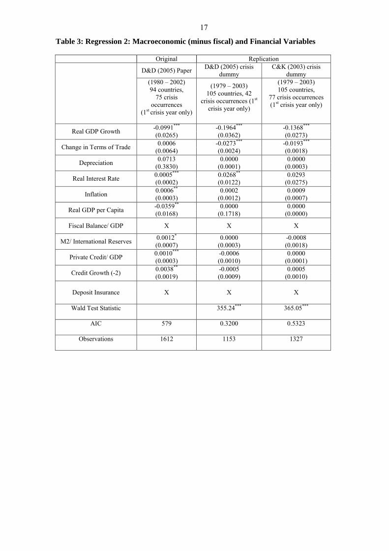
Table 3: Regression 2: Macroeconomic (minus fiscal) and Financial Variables

Original Replication



(1980 � 2002) 94 countries,

75 crisis occurrences

(1st crisis year only)

(1979 � 2003) 105 countries, 42

crisis occurrences (1st crisis year only)

(1979 � 2003) 105 countries,


Real GDP Growth -0.0991***

(0.0265) -0.1964***

(0.0362) -0.1368*** (0.0273)


-0.0273***

(0.0024) -0.0193***

(0.0018)

Depreciation 0.0713 (0.3830)

0.0000 (0.0001)

0.0000 (0.0003)


0.0268**

(0.0122) 0.0293

(0.0275)

Inflation 0.0006**

(0.0003) 0.0002

(0.0012) 0.0009

(0.0007)

Real GDP per Capita -0.0359**

(0.0168) 0.0000

(0.1718) 0.0000

(0.0000)

Fiscal Balance/ GDP X X X

M2/ International Reserves 0.0012* (0.0007)

0.0000 (0.0003)

-0.0008 (0.0018)

Private Credit/ GDP 0.0010*** (0.0003)

-0.0006 (0.0010)

0.0000 (0.0001)

Credit Growth (-2) 0.0038**

(0.0019) -0.0005 (0.0009)

0.0005 (0.0010)



AIC 579 0.3200 0.5323


18

Table 4: Regression 3: Macroeconomic, Financial and Fiscal Variables.




(1980 � 2002) 94 countries,


(1979 � 2003) 105 countries, 42 crisis

occurrences (1st crisis year only)

(1979 � 2003) 105 countries,


Real GDP Growth -0.1115***

(0.0319) -0.1891***

(0.0402)

-0.1677***

(0.0338)

Change in Terms of Trade

-0.0024 (0.0066)

-0.0288***

(0.0030) -0.0150***

(0.0028)


0.0000 (0.0002)

-0.0002 (0.0002)

Real Interest Rate 0.0005***

(0.0002) 0.0313** (0.0128)

0.0034 (0.0138)

Inflation 0.0007**

(0.0003) 0.0002

(0.0014)

-0.0161 (0.0102)

Real GDP per Capita� -0.0414**

(0.0175) -0.0275 (0.0215)

-0.0303**

(0.0147)

Fiscal Balance/ GDP 0.0033**

(0.0016) -0.0498 (0.0348)

0.0402 (0.0314)

M2/ International Reserves

0.0062***

(0.0021) 0.0000

(0.0002)

-0.0001 (0.0004)

Private Credit/ GDP 0.0016***

(0.0004) -0.0007 (0.0010)

0.0000 (0.0001)

Credit Growth (-2) 0.0044* (0.0023)

-0.0004 (0.0010)

-0.0117**

(0.0048)


Wald Test Statistic 293.58***

311.31***

AIC 494 0.3306 0.5276


19

Table 5: Regression 4: All Variables

These regressions (Tables 2-5) show that real GDP growth, real interest rates and real GDP

per capita are consistently and significantly associated with crisis. These results are consistent

with the DD05 findings. However in our case, adding many of the financial variables makes

little difference to the model (the coefficients are not significant) and actually reduce the AIC.

This is in contrast to DD05 who found that increased budget deficits and private credit/ GDP

raised banking crisis probability.




(1980 � 2002) 94 countries,

77 crisis occurrences

(1st crisis year only)

(1979 � 2003) 105 countries, 38

crisis occurrences (1st crisis year only)

(1979 � 2003) 105 countries,


Real GDP Growth

-0.1175***

(0.0332) -0.1925***

(0.0405)

-0.1706***

(0.0340)

Change in Terms of Trade -0.0028 (0.0067)

-0.0302*** (0.0034)

-0.0159***

(0.0030)


0.0000 (0.0002)

-0.0002 (0.0002)


0.0314**

(0.0131)

0.0009 (0.0145)

Inflation 0.0007 (0.0003)

0.0003 (0.0013)

-0.0172*

(0.0105)

Real GDP per Capita� -0.0544*** (0.0184)

-0.0318 (0.0220)

-0.0349**

(0.0154)

Fiscal Balance/ GDP 0.0014** (0.0020)

-0.0496 (0.0352)

0.0440 (0.0318)

M2/ International Reserves 0.0066*** (0.0022)

0.0000 (0.0002)

-0.0001 (0.0005)

Private Credit/ GDP 0.0012*** (0.0005)

-0.0008 (0.0011)

-0.0001 (0.0001)

Credit Growth (-2) 0.0041* (0.0022)

-0.0005 (0.0011)

-0.0120***

(0.0049)

Deposit Insurance 0.5859** (0.2786)

0.3477 (0.3607)

0.3549 (0.2942)


AIC 493 0.3318 0.5283


20

In regression 3, we find inflation may have a weak negative effect on banking crisis which

may reflect procyclical behaviour of asset prices, since during booms, crises are less likely.

The fact that higher real GDP growth is consistently found to reduce banking crisis

probability confirms it is a robust leading indicator of banking crisis. Apart from directly

reducing non-performing loans (and concurrently credit risk), GDP growth may also delay

banking crises, again due to procylicality. The coefficients on real interest rates are positive

and apart from one regression, significant. This suggests interest rate risk materialisation and

financial liberalisation could trigger crises. However the effect of interest rates is not robust to

the banking crisis dummy used; alongside the Caprio and Klingebiel (2003) (CK03) dummy,

interest rates become insignificant. One explanation may the less stringent crisis criteria CK03

use to classify systemic episodes in comparison to DD05. The DD05 crises are more likely to

be fully systemic implying that real interest rates may become a more important trigger if

financial instability is endemic as opposed to more localised insolvency. Lagged real credit

growth is negatively significant in one specification and insignificant in others whereas DD05

found this variable to be significant albeit in one model specification only. Similarly they

found domestic credit/ GDP to be positively associated with crisis, but this variable was not

significant in any of our initial regressions.

In contrast to DD05, we find that positive terms of trade shocks consistently reduce banking

crisis probability. This may be due to the higher number of small open economies in our

sample compared to DD05. Apart from the direct effects on increased loan repayments,

favourable terms of trade are also likely to reduce chances of currency crisis. As Kaminsky

and Reinhart (1999) show, once a banking crisis is underway, the onset of a currency crisis is

likely to deepen banking difficulties.

The Wald test statistics show the coefficients are all significantly different from zero. On the

basis of the AIC it appears the most parsimonious model (regression 1) is the best

specification of the four regressions. However the changing signs on the coefficients and the

insignificance of many variables which DD05 found to be significant indicate the

specification may be improved.

3.2 Improving the Model: Transforming Variables

21

Following the first set of regressions, we experimented with data transformations and lags to

accommodate the dynamics of banking crises. Furthermore, the occurrence of a banking crisis

leaves the economy vulnerable to further crises and may explain the successive crisis episodes

observed in many economies. Omitting observations following crisis onset as in DD05

removes this vulnerability from the data. Hence we repeat the regressions retaining all

observations.

DD05 do not mention heterogeneity of series but inspection of the data shows significant

differences in the magnitude of variables within countries (i.e. between growth and level

variables) and between countries. Accordingly, we standardise each series and log several

variables (other series have been checked for stationarity). The standardising process involves

dividing the deviation of each observation from the pooled mean by the pooled standard

deviation, )(var/)( ,

*

, XXXX titi −= , where tiX ,is the observation for country i at time t, X is

the pooled mean and )(var X is the pooled standard deviation. We remove depreciation since

it is correlated with terms of trade and it was insignificant in the DD05 regressions. Also we

assess for lags in a number of variables, the chosen lags were found from a grid search. Note

in particular that credit growth and deposit insurance take quite long lags prior to the crisis, as

is plausible (i.e. a crisis may be several years after the credit boom�s peak, while deposit

insurance takes time to affect risk-taking behaviour).

Tables 6 shows that more indicators now appear as significant predictors of crisis and more

leading indicators appear robust to the banking dummy specification. Note however that the

lags chosen have also reduced the number of observations compared with Table 5.

Standardising the variables and taking logs where necessary improves significance on many

variables. This suggests that without a fixed effects model, unless data is restricted to a

homogenous country set, some form of adjustment may be necessary to accommodate

variation in the data. This allows a wider cross-country sample to underpin the EWS. We first

discuss the overall significance of the explanatory variables following their transformation

before explaining why we have selected the lags we have and discussing their significance in

the context of banking crisis dynamics in section 3.3.

Real GDP growth remains robustly significantly inversely related to crisis, whichever banking

crisis definition used. High real interest rates now appear to significantly increase the

probability of banking crisis in accordance with DD05. Moreover, the size of the coefficient

22

implies the interest rate risk effect is much stronger in our model. A rise in inflation

substantially increases the chances of crises. Unlike DD05, who did not find this variable to

be significant, we find the inflation coefficient to be the largest of all. A healthy fiscal surplus

seems to signal authorities� general ability to manage policy in a positive sense and their

ability to intervene in the banking system if necessary, which reduces crisis likelihood. The

significance of this variable increases under our specification compared to DD05. Conversely,

the positive coefficient on M2/ Reserves shows an increase in un-backed money adds to the

chances of capital flight and thus to the probability of a pure banking or twin crisis. This

coefficient was insignificant in our previous specifications.

Table 6: Regression 5: All Variables: Standardisation, More Lags and Logs Introduced D&D (2005) crisis

dummy C&K (2003) crisis

dummy

(1979 � 2003) 105 countries, 46 crisis observations (all years)

(1979 � 2003) 105 countries,

81 crisis observations (all crisis years)

Log (Real GDP Growth(-2)) -0.4026***

(0.1443) -0.2978***

(0.1214)


0.0007 (0.0026)

Real Interest Rate (-2) 0.5729*

(0.3499) -0.0354 (0.2851)

Inflation 17.1924***

(4.5638) 3.4592

(3.8379)

Change in Real GDP per Capita -16.6447**

(6.9907) -16.5295***

(5.2466)

Fiscal Balance/ GDP -0.1711***

(0.0525) -0.1238***

(0.0417)

M2/ International Reserves 2.7189**

(1.3164) 1.9731

(1.3653)

Log (Private Credit/ GDP) -0.4394***

(0.1208) -0.3802***

(0.1007)

Credit Growth (-5) 4.2305**

(2.0514) -0.1574 (0.2362)

Deposit Insurance (-10) 0.5755*

(0.3555) 0.1412

(0.2700)


AIC 0.6417 0.9564

Observations 368 368

The negative sign on the private credit/ GDP coefficient indicates that crises are more likely

in lesser-developed economies where bank intermediation is the main mechanism of raising

23

capital and regulation may be of lower quality. The coefficient on credit growth supports the

theory that accumulations in credit risk are a cause of banking crises. The safety net of deposit

insurance significantly raises the likelihood of morally hazardous lending by banks, which

adds to the crisis probability. Again, this effect appears to be much stronger under our

specification compared to DD05. The coefficient on the change in GDP per capita is strongly

negative and significant, indicating that improvements in institutional quality associated with

higher GDP reduce banking crisis risk.

Whilst the above results seem entirely consistent with banking crisis theory, they are not

entirely robust to the choice of baking crisis dummy. Nevertheless, some variables which

were insignificant alongside the CK03 definitions when untransformed data was used

(regressions 1-4) now appear significant under both dummy definitions: fiscal balance/ GDP

and private credit/ GDP. The significance of real GDP per capita now increases for the CK03

dummy in comparison to when data is not standardised. On the other hand, when the CK03

definitions of crisis are used, inflation and credit growth are less significant.

Under the new specification with lags introduced, terms of trade loses significance for both

crisis definitions. This may imply that terms of trade shocks play little part in the

accumulation of systemic risk, but that (as regression 1-4 show), once risk is amassed

systemically, a sudden deterioration in an economy�s terms of trade could precipitate a

banking crisis.

3.3 Improving the Model Further: Investigating Dynamics.

To model the dynamics of banking crises, we now introduce further lags and several

interaction variables so that we use the data to mimic the procyclical build up of risk. Our

banking crisis story unfolds as follows: credit booms are more likely to occur in an

environment which allows imprudent lending, such as following the adoption of deposit

insurance. Hence, after deposit insurance is introduced we expect to see rises in domestic

credit growth being associated with imprudent lending. This may be tempered if agents are

not so reliant on bank intermediation for funds when deposit insurance is installed. To test the

impact of credit growth in the presence of deposit insurance, we interact credit growth and

deposit insurance at different lags. The results in table 7 clearly show the procyclical

behaviour of credit growth. During the boom phase up to four years prior to crisis, credit

growth appears to generate credit risk. From three years prior to crisis, a cyclical downturn

24

seems to occur with the coefficient sign switching so that credit rationing increases the

likelihood of crisis. The fact that the interaction terms are significant (with credit growth

alone insignificant) also demonstrates how moral hazard is more prevalent when deposit

insurance exists so that credit booms generate considerable banking crisis risk.

Table 7: Regression 6: Procyclicality and Moral Hazard D&D (2005) crisis

dummy C&K (2003) crisis

dummy

(1979 � 2003) 105 countries,

70crisis observations (all years)

(1979 � 2003) 105 countries,

100 crisis observations (all years)

Log (Real GDP Growth) -0.1152 (0.1204)

-0.1329 (0.1083)

Change in Terms of Trade 0.0013

(0.0031) 0.0009

(0.0027)

Real Interest Rate 0.0030

(0.3013) 0.0506

(0.2821)

Inflation 5.6593**

(2.7485) -1.6839 (2.9102)

Change in Real GDP per Capita -18.6873***

(6.9503) -18.7623***

(5.9710)

Fiscal Balance/ GDP -0.0466

(0.0361) -0.0843***

(0.0334)

M2/ International Reserves 12.5815***

(4.7478) 5.4025**

(2.7862)

Log (Private Credit/ GDP) -0.2319**

(0.1037) -0.3905***

(0.0941)

Credit Growth*Insurance -6.2798*

(3.5159) -8.3398**

(3.6856)

Credit Growth*Insurance(-1) -10.9812***

(4.2393) -9.2458***

(3.7538)

Credit Growth*Insurance(-2) -8.1842**

(4.1300) -8.5824**

(3.7562)

Credit Growth*Insurance(-3) -2.7540

(2.8714) 0.7778

(3.0085)

Credit Growth*Insurance(-4) 6.4430**

(3.1518) 4.6280

(3.0500)

Credit Growth*Insurance(-5) 7.9458***

(3.1063) 4.7191*

(2.8103)

Credit Growth(-1) -1.3292 (2.5000)

2.4400 (2.3468)

Credit Growth(-2) 2.3022

(2.7396) 4.9375*

(2.6044)

Credit Growth(-3) 0.1518

(1.4265) -1.9288 (1.6528)

Credit Growth(-4) -0.0899 (0.2471)

-0.3865 (0.3933)

Credit Growth(-5) -0.0729 (0.1235)

-0.0251*

(0.0846) AIC 0.7089 0.8722 Wald Statistic 156.07*** 1.35***

Observations 484 484

25

3.3 In Sample Predictive Ability

We now turn to see the relative performances of the different specifications in terms of their

ability to accurately call crises and non-crises episodes. It should be noted that the higher the

probability threshold set for calling a crisis, the higher the probability of Type I errors (failure

to call crisis) and the lower the probability of Type II errors (false alarm). In this regard, we

initially set our threshold much higher than Demirguc-Kunt and Detragiache (1998) who set

their cut off probability at 0.0519. In contrast we set our threshold at 0.5, arguing that from the

policy maker�s perspective, costly intervention on the basis of a crude EWS should be

avoided unless the model seriously calls a crisis (table 8a). However the threshold can be

changed according to a policy maker�s loss function; those that observe a higher historic crisis

frequency or who wish to avoid �potential� crisis at all costs can lower the cut off probability.

Accordingly we re-estimate in sample predictions using a cut-off probability of 0.05 identical

to Demirguc-Kunt and Detragiache (1998). When we reduce our threshold to the Demirguc-

Kunt and Detragiache (1998) level, our models, notably regressions 5 and 6 have dramatically

higher crisis predictive ability (table 8b).

Table 8a: In Sample Predictive Ability: Cut-Off Probability = 0.5

Regression 1 2 3 Our Version Our Version Our Version Probability

cut-off = 0.5 DD05* DD05 CK03 DD05* DD05 CK03 DD05* DD05 CK03 %

crises correct 60 7 13 60 8 15 58 10 9

% no crises correct

67 96 92 70 96 92 70 96 94

% total correct 67 93 87 70 93 87 70 92 89


cut-off = 0.5 DD05* DD05 CK03 DD05* DD05 CK03 DD05* DD05 CK05 %

crises correct 62 10 5 NA 31 34 NA 34 28

% no crises correct

68 96 95 NA 90 80 NA 98 96

% total correct 68 92 89 NA 82 70 NA 89 82

* For DD05 cut-off probability is 0.05

19 They decide this threshold on the basis of the frequency of crisis episodes in their sample.

26

Table 8b: In Sample Predictive Ability: Cut-Off Probability = 0.05


cut-off = 0.05 DD05 DD05 CK03 DD05 DD05 CK03 DD05 DD05 CK03 %

crises correct 60 53 66 60 54 66 58 66 66

% no crises correct

67 78 50 70 78 34 70 76 48

% total correct 67 77 51 70 78 50 70 75 49


cut-off = 0.05 DD05 DD05 CK03 DD05 DD05 CK03 DD05 DD05 CK05 %

crises correct 62 66 66 NA 91 99 NA 91 99

% no crises correct

68 77 45 NA 44 12 NA 32 23

% total correct 68 76 50 NA 50 31 NA 40 39

Table 8(a) shows that with a cut-off probability of 0.5, our models are better at calling non-

crisis periods correctly although the ability to call crisis episodes is substantially lower than

DD05. This is as we would expect given the trade-off between Type I and Type II errors and

the higher cut-off. However once we lower the threshold to the same level as DD05 at 0.05,

our models out-perform the DD05 models in terms of crisis prediction (apart from regressions

1 and 2). This is independent of the crisis dummy used. Moreover, a dynamic model such as

Model 5 is notably better at predicting crisis events with above 90% of crisis episodes being

called correctly.

Both tables also show that given the same threshold, the CK03 crisis dummy generally is

better predicted by these variables that the DD05 dummy. This may be due to the wider

definitions of crisis that CK03 use so that the CK03 dummy is associated with a reduced

ability to call non-crisis periods correctly and therefore a higher chance of Type II errors.

Table 8b shows our models do not appear to lose much in terms of Type II errors when the

cut-off probability is lowered to 0.05 since based on the DD05 dummy, our % of non-crisis

events correctly predicted is marginally higher than the DD05 models. As a result, our models

consistently outperform the DD05 models in term of total correct predictions but only if the

DD05 dummy is used. If the CK03 dummy is used, our models underperform in total; again

this is probably due to the wider crisis definitions of the CK03 dummy which results in

reduced ability to identify non-crisis periods.

27

Overall these results that incorporating dynamics substantially improves crisis predictive

ability with no significant cost in terms of false alarms. It also illustrates the tradeoff of Type I

and Type II errors in logit models.

3.4 Banking crisis prediction using the method of Kaminsky and Reinhart (1999)

Using exactly the same dataset as the previous logit regressions, we now conduct a signal

extraction approach in the manner of Kaminsky and Reinhart (1999), henceforth KR9920. The

KR99 methodology locates the optimal threshold using a common percentile for the cross-

country distribution of each variable. Whilst we will adopt this approach, we also argue that

minimisation of a common percentile may be problematic. If the 20th percentile is chosen as

the optimal threshold across all cross-sections, this is equivalent to the notion that whenever

real GDP growth falls into the lowest 20% of observations in any country, a crisis is

imminent. Whilst for some countries during some time periods this may be reasonably

correct, for other countries it may not; certain countries may undergo structural changes (e.g.

financial liberalisation, move from recession to boom) which generate different distributions

for the indicator and their optimal threshold may differ accordingly. Hence generalisation to a

common percentile threshold may limit the predictive ability of panel based EWS.

Accordingly we test whether country specific and general grid searches give rise to different

optimal thresholds. We then compare the in-sample predictive ability of the two approaches.

To optimise thresholds on the basis of country specific data we compute the NTSR for each

country using a selection of percentiles. We use a forecasting horizon of two years � one year

prior to the crisis and the crisis year itself. Our horizon is considerably more stringent than the

KR99 signalling window which consists of 54 months (18 months before the crisis, an 18

month crisis episode and 18 months after the crisis). We choose a shorter signalling window

because where there are multiple crisis episodes, signalling windows may overlap. Also,

because we use annual data, our signalling window is restricted to yearly increments. The

lowest NTSR given by the threshold corresponding to each country is then aggregated into a

common threshold. Table 9 and Graphs 1-8 show our optimal thresholds (in terms of

percentiles) and the corresponding correct predictions, where �General� refers to the common

percentile approach used by KR99.

20 We therefore abandon the KR99 variable list which is more focused on detecting balance of payments difficulties.

28

Graph 1: REAL GDP GROWTH COUNTRY SPECIFIC THRESHOLD GENERAL THRESHOLD

NTSR for Real GDP Growth

0.49

0.51

0.53

0.55

0.57

0.59

0.61

0.63

10 8 6 4.5 4 3.5 2 1

threshold percentile

NTSR

0.25

0.3

0.35

0.4

0.45

0.5

0.55

0.6

0.65

0.7

20 10 8 6 4.5 4 3.5 2 1

PERCENTILE

NTSR

Graph 2: TERMS OF TRADE COUNTRY SPECIFIC THRESHOLD GENERAL THRESHOLD

0.72

0.74

0.76

0.78

0.8

0.82

0.84

20 10 8 6 4.5 4 3.5 2 1

threshold

NTSR

1

1.05

1.1

1.15

1.2

1.25

1.3

1.35

20 17 15 10 8 5

THRESHOLD

NTSR

29

Graph 3: REAL INTEREST RATE COUNTRY SPECIFIC THRESHOLD GENERAL THRESHOLD

1.07

1.12

1.17

1.22

1.27

1.32

1.37

1.42

20 10 8 6 4.5 4 3.5 2 1

THRESHOLD

NTSR

0.4

0.5

0.6

0.7

0.8

0.9

1

1.1

20 10 8 6 4.5 4 3.5 2 1 0.5

THRESHOLD

NTSR

Graph 4: DEPRECIATION COUNTRY SPECIFIC THRESHOLD GENERAL THRESHOLD

0.55

0.57

0.59

0.61

0.63

0.65

0.67

0.69

0.71

0.73

0.75

20 10 8 6 4.5 4 3.5 2 1

THRESHOLD

NTSR

0.1

0.15

0.2

0.25

0.3

0.35

0.4

0.45

0.5

0.55

20 10 8 6 4.5 4 3.5 2 1 0.5 0.25

PERCENTILE

NTSR

30

Graph 5: INFLATION COUTNRY SPECIFIC THRESHOLD GENERAL THRESHOLD

0.93

0.95

0.97

0.99

1.01

1.03

1.05

1.07

20 10 8 6 4.5 4 3.5 2 1

THRESHOLD

NTSR

0.5

0.6

0.7

0.8

0.9

1

1.1

1.2

20 10 8 6 4.5 4 3.5 2 1

PERCENTILE

NTSR

Graph 6: BUDGET BALANCE COUNTRY SPECIFIC THRESHOLD GENERAL THRESHOLD

0.71

0.72

0.73

0.74

0.75

0.76

0.77

0.78

20 15 10 8 6 4.5 4 3.5 2 1

PERCENTILE

NTSR

0.8

0.85

0.9

0.95

1

1.05

1.1

1.15

1.2

20 15 10 8 6 4.5 4 3.5 2 1

PERCENTILE

NTSR

31

Graph 7: M2 / RESERVES COUNTYR SPECIFIC THRESHOLD GENERAL THRESHOLD

0.85

0.87

0.89

0.91

0.93

0.95

0.97

0.99

1.01

1.03

20 15 10 8 6 4.5 4 3.5 2 1

PERCENTILE

NTSR

0.3

0.4

0.5

0.6

0.7

0.8

0.9

1

1.1

1.2

1.3

20 15 10 8 6 4.5 4 3.5 2 1

PERCENTILE

NTSR

Graph 8: CREDIT / GDP RATIO

COUNTRY SPECIFIC THRESHOLD GENERAL THRESHOLD

1.12

1.14

1.16

1.18

1.2

1.22

1.24

20 15 10 8 6 4.5 4 3.5 2 1

PERCENTILE

NTSR

0.4

0.45

0.5

0.55

0.6

0.65

0.7

0.75

0.8

0.85

20 15 10 8 6 4.5 4 3.5 2 1

PERCENTILE

NTSR

32

Table 9: Comparison of In-Sample Predictive Ability for General and Country Specific Thresholds.

Real GDP Growth Terms of Trade Country Specific General Country Specific General

Optimal Percentile 8 4 10 8 NTSR 0.5904 0.2701 0.7370 1.0284

% crisis correct 12 10 15 7 % no crisis correct 93 97 89 93

% total correct 81 84 76 78 Real Interest Rate Depreciation Country Specific General Country Specific General

Optimal Percentile 4.5 1 4 2.5 NTSR 1.0917 0.4309 0.5667 0.1436


% total correct 80 85 82 84 Inflation Budget Surplus Country Specific General Country Specific General



% total correct 79 83 79 82 M2/ Reserves Credit/ GDP Country Specific General Country Specific General



% total correct 71 84 78 83

The results show there is a big difference between country specific and general thresholds and

that as a result, the optimal percentile differs widely. Using a country specific optimisation

procedure results in a higher percentage of crises being predicted compared to the generalised

threshold method. However, the general threshold procedure is better at calling non-crisis

episodes, so that there are a higher chance of Type I errors with the general method and

conversely, a higher chance of Type II errors with the specific method. Given that there is a

high ratio of non-crisis to crisis observations in the sample, overall the general procedure

performs better in terms of total correct predictions. As a result, the general threshold virtually

always gives a lower NTSR to the specific threshold where values below one indicate the

variables are informative.

In terms of individual leading indicator performance, the best predictors of crisis appear to be

real GDP growth and changes in the terms of trade. This is consistent with the panel logit

33

results. M2/ reserves and budget surpluses are also better than other indicators at calling

crises.

Although we follow the Kaminsky and Reinhart (1999) procedure, we are unable to compare

most of our indicator performances with theirs since they conducted their estimations for a

different sample of countries and different time frames, using mostly different indicators on a

monthly basis21. However comparison of indicators common to our study and theirs (real

interest rates and domestic credit/ GDP) shows our indicators are considerably worse at

calling banking crises correctly compared to theirs. For Kaminsky and Reinhart (1999), real

interest rates are able to call 100% of crises correctly whilst domestic credit/ GDP is able to

call 50% of crises correctly. However the authors do not mention their indicators� ability to

call non-crisis periods correctly or the level of Type II errors that arise with such high

prediction rates.

Overall our results suggest there may be policy implications for the selection of the

optimisation procedure. Policy makers who place emphasis on crisis avoidance may utilise

the country specific approach. However the results also imply that a country specific signal

extraction model, where thresholds are derived from historic data for a single country is more

likely to incorporate more information when selecting the optimal threshold. Much of this

heterogeneity is averaged away when deriving global thresholds. We next turn to investigate

whether combining indicators changes the trade off between Type I and Type II indicators for

our dataset.

3.5 Furthering the Signal Extraction Approach: Composite Indicators

Borio and Lowe (2002) developed the Kaminsky and Reinhart (1999) procedure by

constructing composite indicators22 to extract signals of banking crisis. Their approach is to

select indicators which a priori are thought to contain information for banking crisis

prediction. They then aggregate these variables to generate a composite signal whereby the

indicator is switched on if all constituent variables cross their respective thresholds

simultaneously. Selection of optimal composite thresholds is achieved by a grid search to

21 Kaminsky and Reinhart (1999) base their study on 20 small open economies with a fixed exchange rate or a crawling peg over a period 1970-1995. Their sample contained 26 banking crises, 19 of which were twinned. Because they were investigating balance of payments crises as well as twin crises, the variables they used were predominantly different to ours which are based on the DD05 study. 22 They actually focus on the accumulation of risk by integrating different variables� departures from trend into one composite variable.

34

identify the minimum NTSR. However, the noteworthy difference to the KR99 approach is

that the Borio and Lowe (2002) method implicitly gives more weight to Type II errors, since

they consider the failure to predict crises outweighs the costs of unnecessary intervention.

Their more stringent requirement that all individual indicators in the composite must cross

their thresholds for the composite to signal, means when a crisis is called it is more likely to

happen; the probability of a Type I error is reduced at the cost of higher levels of Type II

errors.

In this section we also generate composite indicators but our method differs from Borio and

Lowe (2002). We do not impose a requirement that all indicators within the composite must

cross their thresholds for the composite to signal. Rather, we construct a composite indicator

in the manner of Kaminsky (1999) which may signal crisis even if some of the individual

indicators have not crossed their thresholds. Although we do not assign any weights to Type I

or II errors, we do construct composites based on the general and specific methodologies

followed in section 3.4. Since these two approaches have been shown to favour Type I and

Type II errors differently, we wish to see if this behaviour persists when we construct

composites. We also investigate whether creating composite indicators affects the

informational content of the indicator.

Kaminsky (1999) constructs the composite (C) by weighting each component variable by the

inverse of its noise to signal ratio (equation 5), where tjS is the signal for variable j at time t

and jω is the noise to signal ratio for variable j.

∑=

=T

1tj

tjS

Cω

��(5)

The Kaminsky (1999) criterion for inclusion in the composite is that the variable must

generate a noise to signal ratio of less than one since this implies the variable contains a

higher proportion of information than noise. In our case, we set stronger criteria; we first

construct a composite indicator using variables that have a noise to signal ratio of 0.5 or less

and then we construct composites using variables where the ratio is 0.75 or less. Table 10 lists

the indicators that qualify for each composite; for the 0.5 cut-off, none of the variables qualify

using the country specific approach and we are left with a composite based on the general

threshold approach. For the 0.75 cut-off we construct two composites based on the general

and country specific approaches.

35

Table 10: Variables Qualifying for the Composite Indicator 0.5 NTSR cut-off 0.75 NTSR cut-off

General General Country Specific Real GDP Growth Real GDP Growth Real GDP Growth Real Interest Rate Real Interest Rate Terms of Trade

Depreciation Depreciation Depreciation M2/ Reserves M2/ Reserves Budget Balance

Domestic Credit/ GDP

Domestic Credit/ GDP

Inflation

Table 11 and Graph 9 show the results for the general and specific approaches based on the

different cut-offs for the NTSRs. In section 3.4 we showed the trade-off between Type I and II

errors when selecting between the general and country specific threshold approach, where the

general (specific) approach reduced Type II errors (Type I errors) at the cost of higher Type I

(Type II) errors. A comparison of the general and specific methods for the composite indicator

based on the NTSR ≤ 0.75 shows that this trade-off persists even if composite indicators are

constructed. Hence the general approach continues to weight Type II errors more heavily

whilst the specific approach remains better for policy makers wishing to avoid unnecessary

intervention costs.

In terms of percentage of crises correctly called, both composites based on the general

approach outperform six of the eight indicators used in section 3.4. On the other hand, the

ability to call non-crisis periods correctly is drastically reduced since the general composite

underperforms against seven of the eight indicators. Similarly, the composite based on the

country specific method outperforms six of the single variables at calling crises but

underperforms all except one in its ability to call non-crisis periods correctly.

The composite method therefore appears to improve crisis prediction whether a country

specific or general threshold approach is used but this occurs at the cost of higher Type II

errors. As a result, the overall percentage observations correctly called deteriorates with both

types of composite so that they outperform only one univariate indicator in this respect. The

composite approach raises Type II errors across the board and the general approach has a

lower chance of Type II errors than the specific approach. Hence, we would expect the

composite method to change the NTSR based on the general approach more than it changes

the specific approach NTSR. The results confirm this since both the general composites are

36

equalised at a NTSR of 0.69 which is higher than virtually all the NTSRs for single indicators

based on the same approach.

Conversely, the specific threshold approach which already yields low Type I errors benefits

from the composite method so that the composite specific threshold approach lowers the

NTSR below that of virtually all the univariate indicators with the same methodology. Graph

9 shows there is a difference in optimal percentile thresholds between the general and country

specific approaches at the 4th percentile and the 10th percentile respectively. However using

different values for the NTSR (0.5 and 0.75) as a criterion for individual indicator acceptance

into the composite makes no difference to the optimal threshold or the optimal NTSR.

To summarise, creating a composite indicator increases the likelihood of correctly calling

crises compared to the univariate approach but raises the chances of false alarms. Although

the general approach benefits in terms of crisis prediction, it is penalised by the higher level of

Type II errors and the NTSR is correspondingly higher than when single variables act as

signallers using the same approach. The gains in crisis identification from using a composite

approach conform to the findings of Borio and Lowe (2002) although these authors found

efficiency increased due to a reduction in Type II errors.

Table 11: Comparison of In Sample Predictive Ability of Composite Indicators Using General and Country Specific Thresholds.

50 NTSR cut-off 75 NTSR cut-off General General Country Specific

Optimal Percentile 4 4 10 NTSR 0.6911 0.6911 0.5541

% crisis correct 7 7 15 % no crisis correct 95 95 88

% total correct 82 82 77

37

Graph 9: Comparison of Noise to Signal Ratios for Composite Indicators

0.5

0.6

0.7

0.8

0.9

1

1.1

1.2

1.3

20 15 10 8 6 4.5 4 3.5 2 1

Percentile Threshold

Nois

e to

Sig

nal R

a

general approach (75% cutoff0 specific approach (75% cutoff)general approach (50% cutoff)

3.6 Comparison of the Signal Extraction and Multivariate Logit Models.

On the basis of in-sample predictive ability, the multivariate logit model outperforms the

signal extraction approach in terms of the percentage of crises correctly predicted. Even the

best leading indicator in the signal extraction approach (M2/ Reserves) is able to call only

23% of crises correctly, whereas our dynamic multivariate models (regressions 5 and 6) are

able to call an average of 32 % of crises, despite us setting our cut-off probability much

higher than DD05 and well over 90% of crises using their 0.05 probability.

Berg and Pattillo (1999) who conducted a comparison of multivariate probit and signal

extraction EWS for currency crisis prediction also found the multivariate approach

outperformed the univariate method. With the signal extraction approach, every indicator

misses a substantial number of crises. Berg and Pattillo (1999) suggest this is because the

signal extraction process assumes that a threshold for a variable is a discrete value and that

whenever this is crossed, a crisis becomes impending. In actual fact, as graphs 1-8 show, the

NTSRs �jump� between thresholds so that there is no smooth relationship between threshold

and crisis probability, something that Berg et al (2004) also note. If the NTSR jumps at

different threshold for different countries, then using cross-country data to derive a common

threshold may not be fruitful; the threshold that minimises the NTSR will fall on either side of

the individual optimal thresholds for most countries. In this case, the percentage of crises

38

correctly called will be sub-optimal compared to where threshold are analysed for individual

countries.

The multivariate logit on the other hand, assumes a specific smooth non-linear form for the

relationship between crisis probability and variable behaviour. As the results suggest, this may

be closer to the truth of banking crises, especially once dynamics are taken into account and

given that a large number of crisis episodes across many countries are being assessed

simultaneously for both models.

Even if indicators are aggregated to a composite, the percentages of crises predicted do not

match the dynamic multivariate logit models, although percentage crisis prediction improves.

An alternative approach to ours would be the Borio and Lowe (2002) methodology where

individual variable thresholds are jointly evaluated. In this sense, composite indicator ability

to predict crises is more comparable to the multivariate logit model than the univariate signal

extraction procedure so the two procedures could be compared on the same dataset. This is a

subject of further research for banking crisis prediction.

4 Conclusion

A comparison of the multinomial logit and signal extraction procedures shows that real GDP

growth and terms of trade are robust leading indicators of banking crisis for our

comprehensive sample. Results for other variables are mixed in terms of robustness and as

comparison with the DD05 model shows, results vary according to the dataset used and the

banking crisis definition adopted. Moreover, given the same dataset we show that the choice

of estimation techniques makes a difference in terms of indicator performance and crisis

prediction. Where a multinomial logit is used, transformations which take into account cross-

country heterogeneity may improve model specification since the use of logit prevents fixed

effects estimation. Where a signal extraction procedure is used, optimising thresholds country

by country improves ability to correctly predict crises. Creating composite indicators may

further improve crisis prediction. Hence the use of the multinomial logit model may be better

suited to a global EWS whereas the signal extraction approach may be better suited to country

specific EWS.

We also show that dynamics of banking crises are an extremely important consideration when

designing an EWS since procyclical variables may have an independent effect on banking

39

crisis and a joint effect with institutional factors. In such cases the sequencing of institutional

reforms and procyclical movements in credit and real GDP growth become important. Using

contemporaneous data for all variables ignores the build up of financial instability that arises

from the procyclical behaviour of many indicators. Once we took theory into account and

used the data to incorporate a more realistic story of crisis, indicator significance improved.

Despite a much higher probability threshold than the DD05 study, our logit model was able to

call a significant proportion of crises correctly.

As noted, international financial institutions do not employ an EWS specifically for banking

crisis. However, given the ongoing liberalisation of emerging market financial sectors as well

as the changing nature of banking risks as more economies move into market and securitised

banking phases, the use of EWS for crisis prevention is more necessary than ever. As we have

shown, it is important to consider the policy maker�s objectives when designing predictive

models since there is a trade of between correctly calling crises and false alarms. In this sense

our study confirms that EWS for banking crises are a necessary but not sufficient tool for

predicting further crisis episodes, since a generalised global model cannot be a substitute for

country-specific macroprudential surveillance.

References:

Berg, Andrew and Pattillo, Catherine, (1999)."Predicting currency crises: The indicators approach and an alternative," Journal of International Money and Finance, Elsevier, vol. 18(4), pages 561-586, August. Berg, Andrew, Borensztein, Eduardo and Pattillo, Catherine, (2004). �Assessing Early Warning Systems: How Have They Worked In Practice?� IMF Working Paper, WP/04/52, International Monetary Fund, Washington. Borio, Claudio, Craig Furfine, and Philip Lowe (2001) 'Procyclicality of the financial system and financial stability: issues and policy options,' BIS Papers No. 1, BIS. Borio, Claudio and Lowe, Philip (2002). �Assessing the Risk of Banking Crisis�, BIS Quarterly Review, December 2002. Caprio, Gerard and Klingebiel, Daniela, (July 1996). "Bank Insolvencies: Cross-Country Experience". World Bank Policy Research Working Paper No. 1620. Caprio, Gerard and Daniela Klingebiel, (2003). �Episodes of Systemic and Borderline Financial Crises.� World Bank Research Dataset. Chan, Getmansky, Haas and Lo (2006). �Systemic Risk and Hedge Funds�, in �The Risks of Financial Institutions�, (p. 235-330), University of Chicago Press. Chari, V V and Jagannathan, Ravi, (1988) " Banking Panics, Information, and Rational Expectations Equilibrium," Journal of Finance, American Finance Association, vol. 43(3), pages 749-61, July. Craig R S, Davis E P and Garcia A (2005), "Sources of procyclicality in East Asian financial systems", in eds S Gerlach and P Gruenwald, �Procyclicality of financial systems in Asia�, Palgrave McMillan

40Das, Udaibir, Quintyn, Marc, G, and Chenard, Kina (2004). �Does Regulatory Governance Matter for Financial System Stability? An Empirical Analysis �. IMF Working Paper No. 04/89, International Monetary Fund, Washington. Davis, E Phillip (1995). �Debt, Financial Fragility and Systemic Risk�. Oxford University Press. Davis E P (1999), "Russia/LTCM and market liquidity risk", The Financial Regulator, 4/2, Summer 1999, 23-28 Davis E P and Zhu H (2004), "Bank lending and commercial property prices, some cross country evidence", BIS Working Paper No 150 Davis E P and Zhu H (2005), "Commercial property prices and bank performance", BIS Working Paper No 175 Demirguc-Kunt, A. and Detragiache, E. (1998). �The Determinants of Banking Crises in Developed and Developing Countries�. IMF Staff Paper, Vol. 45, No. 1, International Monetary Fund, Washington. Demirguc-Kunt, Asli & Detragiache, Enrica, (2002). "Does deposit insurance increase banking system stability? An empirical investigation," Journal of Monetary Economics, Elsevier, vol. 49(7), pages 1373-1406, October. Demirgüç-Kunt, Asli and Detragiache, Enrica (2005). "Cross-Country Empirical Studies of Systemic Bank Distress: A Survey." IMF Working Papers 05/96, International Monetary Fund. Diamond D. and Dybvig P. (1983). �Bank runs, deposit insurance and liquidity�. Journal of Political Economy, 91, 401-19. Eichengreen, B. and Arteta C. (2000). �Banking Crises in Emerging Markets: Presumptions and Evidence�. Centre for International Development and Economics Research Working Paper, C00-115, August. Eichengreen, Barry and Rose, Andrew K. (1998). "Staying Afloat When the Wind Shifts: External Factors and Emerging-Market Banking Crises," NBER Working Papers 6370, National Bureau of Economic Research, Inc. Ergungor, E and Thompson, James (2005). �Systemic Banking Crises�, Policy Discussion Papers, Federal Reserve Bank of Cleveland, Number 9, February 2005. Federal Deposit Insurance Corporation (1997). �Commercial Real Estate and the Banking Crises of the 1980s and Early 1990s�. In �An Examination of the Crises of the 1980s and Early 1990s�, Volume 1, Chapter 3, FDIC. George, E. A. J. (1998). �The New Lady of Threadneedle Street�. Governor�s Speech, Bank of England, London, February 24. Glick, Reuven and Hutchison, Michael (1999). "Banking and currency crises; how common are twins?," Proceedings, Federal Reserve Bank of San Francisco, issue Sep. Gonzalez-Hermosillo, Brenda (1999). �Developing Indicators to Provide Early Warnings of Banking Crises�. Finance and Development, Volume 36, Number 2, IMF Publications, Washington. Gorton, G. (1988). �Banking Panics and Business Cycles�. Oxford Economic Papers, Vol. 40, pp 751-781. Gourinchas, Pierre-Olivier, Valdes, Rodrigo and Landerretche, Oscar, (2001). "Lending Booms: Latin America and the World." NBER Working Papers 8249, National Bureau of Economic Research, Inc. Greene, W. H. (2000). �Econometric Analysis.� Prentice Hall International, Co., London, UK . Hardy, Daniel C. L. and Pazarbasioglu, Ceyla (1998). "Leading Indicators of Banking Crises-Was Asia Different?," IMF Working Papers 98/91, International Monetary Fund. Herring, Richard J. and Wachter, Susan M. (1998). "Real Estate Cycles and Banking Crises: An International Perspective". Zell/Lurie Center Working Papers 298, Wharton School Samuel Zell and Robert Lurie Real Estate Center, University of Pennsylvania. Hoggarth, Glen and Saporta, Victoria (2001). �Costs of Banking System Instability: Some Empirical Evidence.� June, Financial Stability Review.

41Honohan, Patrick, (2000). "How Interest Rates Changed under Financial Liberalization: A Cross-Country Review ". World Bank Policy Research Working Paper No. 2313. Jacklin, C. and Bhattacharya, S. (1988). �Distinguishing Panics and Information-Based Bank Runs: Welfare and Policy Implications�. Journal of Political Economy, vol. 96(3), pages 568-92, June, University of Chicago Press. Kaminsky, Graciela (1999). �"Currency and Banking Crises: The Early Warnings of Distress". IMF Working Paper No. 99/178. Kaminsky L.G. and Reinhart C.M. (1999). �The twin crises; the causes of banking and balance of payments problems�. The American Economic Review, Vol. 89, No. 3, pp 473-500. Kaufman, George, G. and Scott, Kennneth, E. (2003). �What is Systemic Risk and Do Bank Regulators Retard or Contribute to It?� The Independent Review, Volume 7, Number 3, Winter 2003. Lindgren Carl-Johan, Garcia, Gillian and Saal, Matthew, (Eds.) (1996). �Bank Soundness and Macroeconomic Policy�. International Monetary Fund, Washington. Mckinnon, Ronald, I. (1973). �Money and Capital in Economic Development.� Washington, Brookings Institution. Naude, Willem (1996). �Financial liberalisation and interest rate risk management in Sub-Saharan Africa�, Working Paper, Centre for the Study of African Economies, Oxford, WPS/96.12. Oviedo, Pedro Marcelo (2004). "Macroeconomic risk and banking crises in emerging market countries: business fluctuations with financial crashes," Proceedings, Federal Reserve Bank of San Francisco, issue Jun. Santos, Joao (2000). �Bank Capital Regulation in Contemporary banking Theory: A Review of the Literature�. BIS Working Papers, No. 90, September 2000, Bank of International Settlements. Stiglitz, Joseph (1994). �The Role of the State in Financial Markets�, in Bruno and Peskovic eds. Proceedings of the World Bank Annual Conference on Development Economics, Washington, World Bank.

42

APPENDIX: Country List Algeria India Switzerland Antigua/Barbuda Indonesia Syria Argentina Ireland Tanzania Australia Israel Thailand Austria Italy Togo Bahamas Jamaica Trinidad and Tobago Bahrain Japan Tunisia Bangladesh Jordan Turkey Barbados Kenya Uganda Belgium Korea UK Bolivia Laos Ukraine Botswana Lebanon Uruguay Brazil Madagascar USA Burundi Malaysia Venezuela Cameroon Mali Vietnam Canada Mauritius Zambia Chile Mexico Zimbabwe Colombia Mozambique Congo Myanmar Costa Rica Nepal Cyprus Netherlands Czech Republic New Zealand Denmark Nicaragua Dominica Niger Dominican republic Nigeria Ecuador Norway Egypt Panama El Salvador Papua New Guinea Equatorial Guinea Paraguay Ethiopia Peru Finland Philippines France Poland Germany Portugal Ghana Romania Greece Russia Grenada Senegal Guatemala Seychelles Guinea Bissau Sierra Leone Guyana Singapore Haiti South Africa Honduras Spain Hong Kong Sri Lanka Hungary Swaziland Iceland Sweden

COMPARING EARLY WARNING SYSTEMS FOR …ephilipdavis.com/earlywarning.pdfCOMPARING EARLY WARNING...

Documents

Transcript of COMPARING EARLY WARNING SYSTEMS FOR …ephilipdavis.com/earlywarning.pdfCOMPARING EARLY WARNING...