COMPARATIVE STUDY OF STREAM FLOW PREDICTION MODELS … · COMPARATIVE STUDY OF STREAM FLOW...

139

Int. J. LifeSc. Bt & Pharm. Res. 2012 S R Asati and S S Rathore, 2012

COMPARATIVE STUDY OF STREAM FLOWPREDICTION MODELS

S R Asati1* and S S Rathore1

Research Paper

Stream flow prediction is required to provide the information of various problems related to thedesign and effective operation of river balancing system. The evaluation of natural and technicalscience over the past centuries has been closely related to experimental studies and modelingof natural resources. Methods to continuously predict water levels at a site along a river aregenerally its model based. Hydrologist has relied on individual techniques such as determinates,stochastic, conceptual or black box type to model the complex, uncertain rainfall and consecutivewater levels. These techniques provide reasonable accuracy in modeling and prediction of streamflow. River Wainganga has been subjected to water level rise during 2004-2005 and, consequently,the low-laying areas along the bank are in undated, giving problems to local inhabitants, irrigationactivities and people properly. Another river Bagh has been connecting to the said river theproblem of flood arises more. Therefore predicting water levels has started to attract the attentionof the researchers. How this local problem get solved or minimized? An attempt has been madeto use the conventional method such as Autoregressive model, more deterministic approachthrough multi-Linear Regression model and Artificial Neural Network which is capable of identifyingcomplex non-linear relationship between input and output data without attempting to reachunderstanding into the nature of the process. The performances of these approaches werecompared and the best possible result amongst them is the key point of this study.

Keywords: Artificial neural network, Runoff, River, Auto-regressive, Multi-linear regression

*Corresponding Author: S R Asati, [email protected]

ISSN 2250-3137 www.ijlbpr.comVol. 1, No. 2, April 2012

© 2012 IJLBPR. All Rights Reserved

Int. J. LifeSc. Bt & Pharm. Res. 2012

1 Department of Civil Engineering, MIET, Gondia 441614, Maharashtra State.

INTRODUCTIONWater is not lost in undergoing various processes

of hydrological cycle namely, evaporation,

condensation, rainfall, stream flow etc., but gets

converted from one form to another was known

during the Vedic period. Prediction of rainfall

quantity in advance by observation of

natural phenomenon is illustrated Puranas,

Vrahatsamhita (550A.D.), Meghmala (900A.D.),

and reference of rain gauges is available in

Arthshashtra of Kautilya (400B.C.) and Astadhyali

of Panini (700 BC). The quantity of rainfall in

various parts of India was also known to Kautilya.

It means ancient books also reflect the

140


importance and the high stage of development of

water resources and hydrology in ancient India.

Stream flow predictions for a particular section

are required in order to do the attentiveness

against the un-avoidable situation when the water

level rises. The situation may cause due to

improper operation and lack of co-ordination

between the human beings who are directly or

otherwise indirectly involved in the process of

controlling the hydraulic structures. Such stream

flow predictions are invariably based on

observation of rainfall on the upper catchment,

often supplemented by rainfall the intervening

catchment. The quantities of water prediction are

obtained in real time, by using a model to

transform the input functions of time. These can

be upgraded, modified considering the errors

observed in previous prediction up to the time of

making the forthcoming prediction. It has a wide

spectrum of applicability for the recent and future

planning field and the important factor in the

sustainable management of water resources.

The huge amount of water in the rainy season

destructs the mind as well as path of the rivers. If

a river flows with its peak discharge, another river

meet at a certain point with full of discharge, then

what will happen and Up to what extent?

The proper balance is needed to minimize the

losses related with the human beings as well as

other all formal and informal barriers. To

overcome the cause effective modeling must be

adopted. This can be sorted out by using the best

possible, efficient and effective water resources

system. Various types of models being used to

solve the above said problem, these can be

broadly grouped as deterministic models,

stochastic or statically models, neural network

based model, conceptual or lumped parameters

or simplified physical model and distributed

physical models. Of these, some are data

dependence and some requires physical

information about the systems as in the case of

conceptual model.

Morocho and Hart (1964) connected upon the

growth of two distinct approaches to the problem

of establishing the relationship between rainfall

and stream flow which they referred to as physical

hydrology and system investigation. The former

term was used to describe investing into the

behaviour of interdependence between

hydrological processes, the long term objective

being a complete synthesis of the hydrological

cycle. The progress achieved with this approach

has materially assisted with the development of

hydrological model that are both physically based

and spatially distributed.

The ANN is advantageous because even if the

exact relationship between sets of input and

output data is unknown but is acknowledged to

exist, the network can be trained to learn that

relationship, required on a prior knowledge of

catchment characteristics. In the hydrological

context, the input pattern consist of rainfall depths

and the output the discharges at the catchment

outlet. Since the contributions from different parts

of the catchment arrive at the outlet of different

times, the variations in the discharge output may

be considered to be determined by rainfall depths

at both the concurrent and previous time

intervals. Preliminary work (Hall and Mines, 1993)

has indicated that the number of antecedent

rainfall ordinates required is broadly related to the

lag time of the drainage area. Since the ANN

relates the pattern of inputs to the pattern of

output, volume continuity is not a constraint.

AIM OF STUDYThe aims of this study are to develop prediction

141


models as a tool to predict the flows, are as under.

• To develop AR model for conventional

approach for runoff based lead time runoff

prediction of Wainganga sub basin under

Godavari basin.

• To develop MLR model for deterministic

approach for runoff based lead time runoff

prediction of said basin.

• To develop ANN model for runoff based lead

time runoff prediction for same basin.

• To study the effect of input patterns on runoff

prediction.

• To carry out performance evaluation of

developed models using different performance

criteria.

• Comparison of above developed models.

HYDROLOGICAL MODELCLASSIFICATIONHydrological models are commonly classified as

physical models and abstract models. Physical

models include scale models like hydraulic

models of a spillway, analog models which use

another physical system having properties similar

to those of the real system. Abstract models

shows the system in mathematical form. The

system operation is described by a set of

equations &logical statements. A mathematical

model can also be transformed to a computer

programme describing an algorithm for the

system. Almost all useful hydrological models are

in fact implemented as computer programmes.

The models are classified according to three

important criteria such as, a) Randomness

(deterministic or stochastic), b) Spatial variation

(lumped or distributed), and c) Time variability

(time- dependent, time independent).The

simplest type of model will be a deterministic

lumped time-independent model. The most

complex type of model would be a stochastic

model with space variation in three dimensions

and with time variation.

LINEAR REGRESSION MODELSRegression is the procedure of establishing

relationship between two variables, referred to as

the response variable “y” (dependent variable), &

the explanatory variable “x” (independent variable).

Simple Linear Regression Models referred to as

the linearity of the variables associated with the

problem. Regression is performed in order to, i)

Learn something about the relationship between

the two variables, ii) Remove a portion of the

variation in one variable in order to gain a better

understanding of some other, more interesting

portion of the variation, and iii) predict values of

one variable for which data are available.

MULTIPLE LINEARREGRESSIONS (MLR)MLR is the extension of Simple Linear Regression

to the case of multiple explanatory variables. MLR

is the procedure of establishing relationship

between a dependent variable “y”& set of

independent variables x1, x

2, x

3...xn, governing a

phenomenon. In hydrological application, runoff

is considered to be dependent on rainfall at

different stations; runoff at a particular station

depends on runoff at upstream gauging stations,

runoff at current time step & previous time step

as independent variables with runoff at future time

step as dependent variable etc.

STOCHASTIC MODELSIn order to evaluate a new sophisticated model

can be applied to approximate the relationship

142


between a set of inputs and a set of outputs, it is

necessary to compare the predictive capabilities

of new model with the existing approaches. The

comparison of models is usually accomplished

by testing all the models of interest on a data set

from the same watershed.

There are varies regression models like Auto

Regressive {AR (p)}, Auto Regressive Moving

Average {ARMA (p,q)}and Auto Regressive

Integrated Moving Average {ARIMA (p,d,q)} based

on their p,q and d. Since the data available for the

present study is non- stationary, the basic

requirement to develop the AR and ARMA models

could not be satisfied. The ARIMA time series

analysis uses lags and shifts in the historical data

to uncover patterns (e.g. moving averages,

seasonality) and predict the future values. The

ARIMA model was first developed in the late 60s

but it was systemized by Box and Jenkins (1976).

ARIMA is more complex to use than other

statistical prediction techniques but quite powerful

and flexible.

ARTIFICIAL NEURAL NETWORKThe human brain contains billions of

interconnected neurons. Due to the structure in

which the neurons are arranged and operate,

humans are able to quickly recognize patterns

and process data. An ANN is a simplified

mathematical representation of this biological

neural network. It has the ability to learn from

examples, recognize a pattern in the data, adapt

solutions over time, and process information

rapidly.

Rumelhart et al. (1986) first introduced back

propagation algorithm based on gradient descent

search optimization. It is particularly useful as

pattern-recognition tools for generalization of

input-output relationships. The most common

application in water resources includes those for

rainfall runoff relationships and stream flow

prediction.

ANNs are structured is intimately linked with

the learning algorithm used to train the network.

A typical ANN consists of a classifying neural

network is by the number of layers: single

(Hopfield nets), bi-layer (Adaptive Resonance

nets) and multi-layer (most back propagation

nets). ANNs can also be categorized based on

the direction of information flow and processing.

In a Feed Forward Network, the nodes are

generally arranged in layers, starting from a first

input layer and ending at the final output layer.

There can be several hidden layers, with each

layer having one or more neurons. Information

passes from the input to the output side. The

neurons in one layer are connected to those in

the next, but not to those in the same layer. Thus,

the output of a neuron in a layer is dependent

only on the outputs it receives from previous

layers and the corresponding weights. On the

other hand, in a recurrent or feedback ANN, is

vice-versa. This is generally achieved by recycling

previous network outputs as current inputs, thus

allowing for feedback. Sometimes, lateral

connections are used where neurons within a

layer are also connected. ANN formulation stages

are tabulated in “Figure .1”.

STUDY AREA AND DATAPREPARATIONGeneral

The present study emphasizes on runoff-based

runoff prediction for Wainganga River sub-basin

under Godawari basin. Strom information is

obtained from Keolari gauging station. Multiple

Linear Regression (MLR), Autoregressive (AR)

143


and Artificial Neural Network (ANN) models were

used for runoff-based runoff prediction.

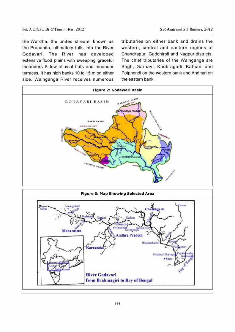
DETAILING OF RIVER BASINSWainganga River sub-basin under Godavari basin

was taken for runoff based runoff forecasting.

Storm values are collected from Keolari gauging

station on Wainganga River. Figures 2 and 3

shows the map of Godavari basin and selected

area respectively.

Wainganga is a river of India, which originates

about 12 km. from Mundara village of

Seoni district in the southern slopes of

the Satpura Range of MP and flows south

through MP and Maharashtra in a very widening

course of approximately 360 miles. After joining

Figure 1: Stages in ANN Formulation

Information Analysis

Stream Flow and Data Series

Statistical Data Analysis

Selection of Neurons in Output Layer

Stream Flow and Data Series

Identification of Pairs for Training and Testing sets

Specification of Model Types

Model Candidates

Statistical Calculation and Analysis of Errors

Evaluation of Model Behavior

Learning and Training Strategy

Model Testing

Comparison of Validation Results

Optimal ModelSelection of

Optimal Model

Lear

ning

Pro

blem

Iden

tific

atio

n P

robl

em

Sele

ctio

n In

put-

Out

put

Pai

rs P

robl

em

Sele

ctio

n In

put

Prob

lem

Dat

a C

onst

itue

ncy

Prob

lem

144


the Wardha, the united stream, known as

the Pranahita, ultimately falls into the River

Godavari. The River has developed

extensive flood plains with sweeping graceful

meanders & low alluvial flats and meander

terraces. It has high banks 10 to 15 m on either

side. Wainganga River receives numerous

tributaries on either bank and drains the

western, central and eastern regions of

Chandrapur, Gadchiroli and Nagpur districts.

The chief tributaries of the Wainganga are

Bagh, Garhavi, Khobragadi, Kathani and

Potphondi on the western bank and Andhari on

the eastern bank.

Figure 2: Godawari Basin

Figure 3: Map Showing Selected Area

145


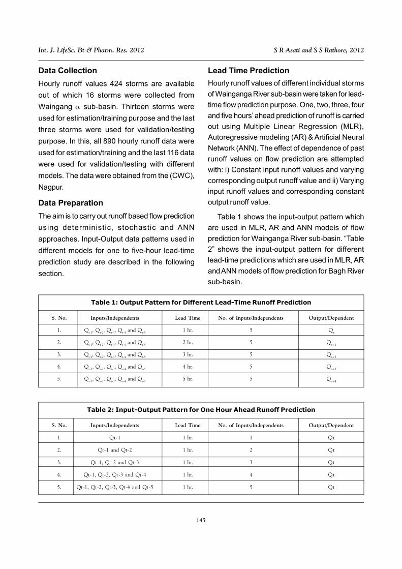
Data Collection

Hourly runoff values 424 storms are available

out of which 16 storms were collected from

Waingang sub-basin. Thirteen storms were

used for estimation/training purpose and the last

three storms were used for validation/testing

purpose. In this, all 890 hourly runoff data were

used for estimation/training and the last 116 data

were used for validation/testing with different

models. The data were obtained from the (CWC),

Nagpur.

Data Preparation

The aim is to carry out runoff based flow prediction

using deterministic, stochastic and ANN

approaches. Input-Output data patterns used in

different models for one to five-hour lead-time

prediction study are described in the following

section.

Lead Time Prediction

Hourly runoff values of different individual storms

of Wainganga River sub-basin were taken for lead-

time flow prediction purpose. One, two, three, four

and five hours’ ahead prediction of runoff is carried

out using Multiple Linear Regression (MLR),

Autoregressive modeling (AR) & Artificial Neural

Network (ANN). The effect of dependence of past

runoff values on flow prediction are attempted

with: i) Constant input runoff values and varying

corresponding output runoff value and ii) Varying

input runoff values and corresponding constant

output runoff value.

Table 1 shows the input-output pattern which

are used in MLR, AR and ANN models of flow

prediction for Wainganga River sub-basin. “Table

2” shows the input-output pattern for different

lead-time predictions which are used in MLR, AR

and ANN models of flow prediction for Bagh River

sub-basin.

S. No. Inputs/Independents Lead Time No. of Inputs/Independents Output/Dependent

1. Qt-1, Qt-2, Qt-3, Qt-4 and Qt-5 1 hr. 5 Qt

2. Qt-1, Qt-2, Qt-3, Qt-4 and Qt-5 2 hr. 5 Qt+1




Table 1: Output Pattern for Different Lead-Time Runoff Prediction

S. No. Inputs/Independents Lead Time No. of Inputs/Independents Output/Dependent

1. Qt-1 1 hr. 1 Qt

2. Qt-1 and Qt-2 1 hr. 2 Qt

3. Qt-1, Qt-2 and Qt-3 1 hr. 3 Qt

4. Qt-1, Qt-2, Qt-3 and Qt-4 1 hr. 4 Qt

5. Qt-1, Qt-2, Qt-3, Qt-4 and Qt-5 1 hr. 5 Qt

Table 2: Input-Output Pattern for One Hour Ahead Runoff Prediction

146


MODEL DEVELOPMENTWainganga Sub-Basin

The main aim of the present research work is to

carry out runoff based flow prediction using three

different prediction approaches such as

Deterministic, Stochastic and ANNs. Three

different models like Multiple Linear Regression

(MLR), Autoregressive (AR) and Artificial Neural

Network (ANN) were developed for flow-prediction

of Wainganga River sub-basin under Godavari

basin.

Multiple Linear Regression Model

Multiple Linear Regression model with different

input-output patterns of two and three hour lead-

time/warning time runoff prediction for Wainganga

River is shown in “Table 3”.

Table 3: Multiple Linear Regression ModelDescription: Wainganga Sub-Basin

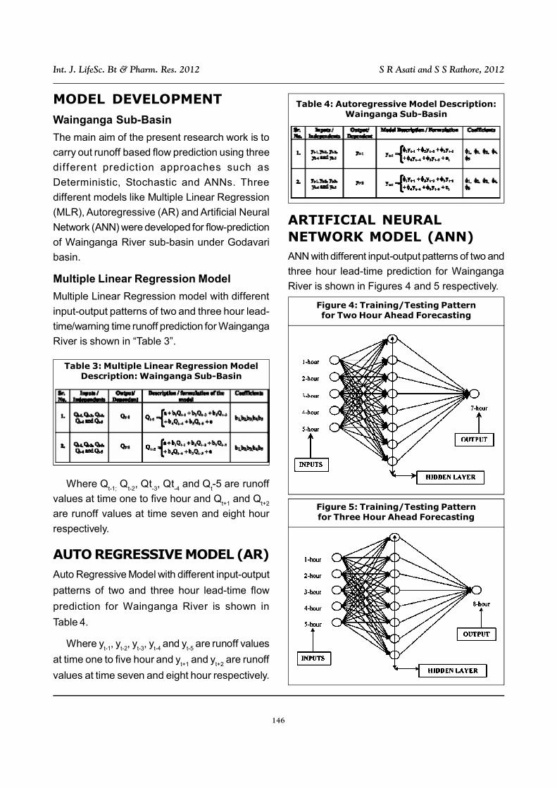
Table 4: Autoregressive Model Description:Wainganga Sub-Basin

Where Qt-1;

Qt-2

, Qt-3, Qt

-4 and Q

t-5 are runoff

values at time one to five hour and Qt+1

and Qt+2

are runoff values at time seven and eight hour

respectively.

AUTO REGRESSIVE MODEL (AR)Auto Regressive Model with different input-output

patterns of two and three hour lead-time flow

prediction for Wainganga River is shown in

Table 4.

Where yt-1

, yt-2

, yt-3

, yt-4

and yt-5

are runoff values

at time one to five hour and yt+1

and yt+2

are runoff

values at time seven and eight hour respectively.

ARTIFICIAL NEURALNETWORK MODEL (ANN)ANN with different input-output patterns of two and

three hour lead-time prediction for Wainganga

River is shown in Figures 4 and 5 respectively.

Figure 4: Training/Testing Patternfor Two Hour Ahead Forecasting

Figure 5: Training/Testing Patternfor Three Hour Ahead Forecasting

147


ANNs configuration, parameters and activation

functions used in the model for Wainganga River

sub-basin are given in Tables 5, 6 and 7

respectively.

Layer No. of Layers No. of Neurons in a Layer

Input 1 5

Hidden 1 8

Output 1 1

Table 5: ANNs Configuration

Parameter Parameter Value

Learning Rate 0.1

Momentum factor 0.1

Table 6: ANNS Parameters

Function Type Function Used

Network Type Feed Forward

Learning Function Back propagation With momentum

Update Function Topological Order

Weights Randomize

Table 7: ANNs Functions

MODELS APPLICATIONMultiple Linear Regressions

Three important approaches like Deterministic,

Stochastic and Artificial Neural Network were

considered. Models such as Multiple Linear

Regression, Auto Regression and Feed Forward

Neural Network were developed for the flow

prediction using hourly runoff values collected

Table 8: MLR Coefficients and Constant: Wainganga Sub-Basin

Lead Time b1 b2 b3 b4 B5 Constant

1-Hour –0.00750 0.005180 0.20408 –0.17235 0.853446 30.179

2-Hour –0.15873 0.128288 0.15214 0.088789 0.555063 60.593

3-Hour –0.12755 –0.04846 0.21831 0.082495 0.561105 81.0432

4-Hour –0.03795 –0.09137 0.05609 0.130349 0.558766 98.745

5-Hour –0.03807 –0.00124 0.01225 –0.031291 0.604362 116.362

from Keolari gauging station on Wainganga River

sub-basin under Godavari basin. One, two, three,

four and five hours’ ahead prediction of

Waingangasub basin was carried out using MLR,

AR and ANNs. A well-known spread-sheet EXCEL

was used for MLR model. Regression analysis

option available in data analysis tools option was

explored. MLR coefficients and constant are listed

in Table 8.

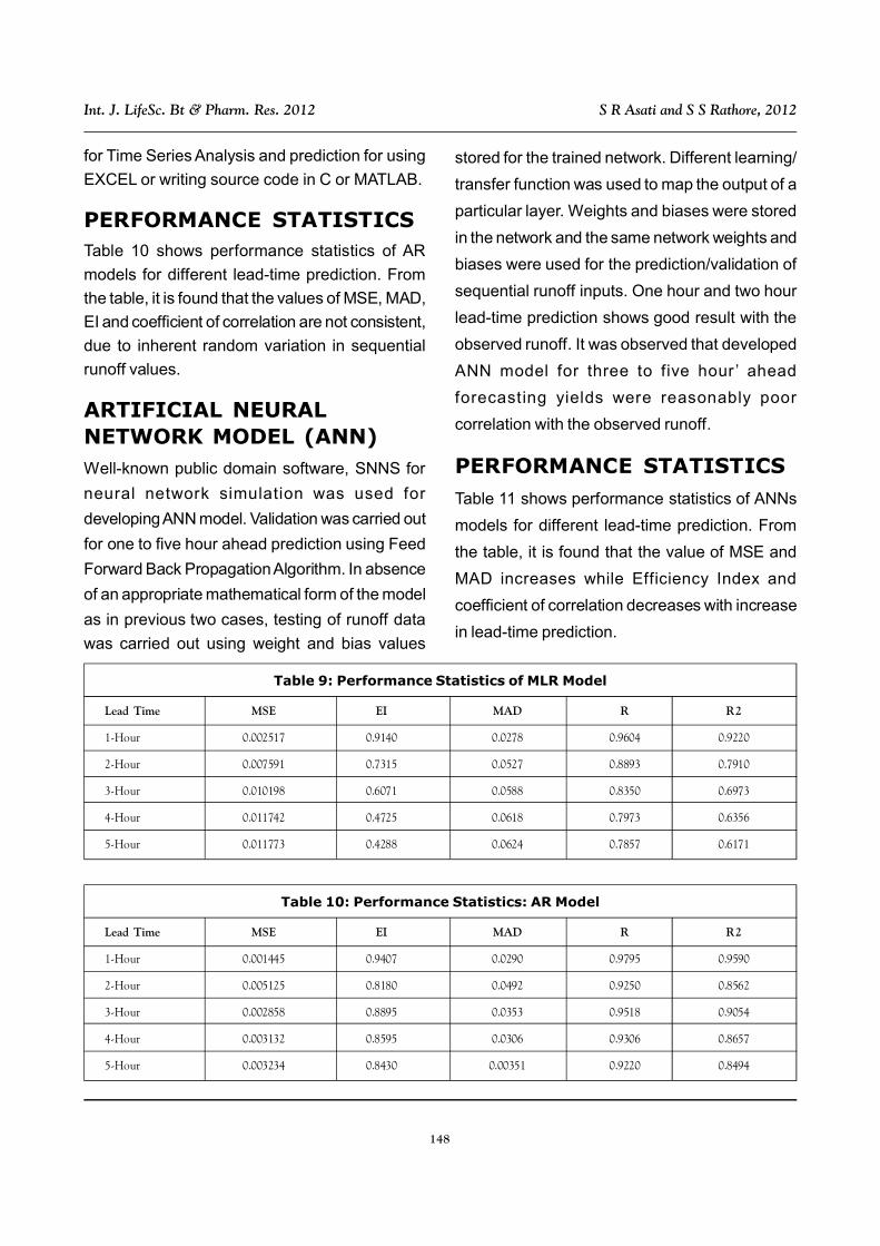
PERFORMANCE STATISTICSThe performance of developed model can be

evaluated with different performance statistics like

Mean Square Error (MSE), Efficiency Index (EI),

Mean absolute deviation (MAD), Coefficient of

Correlation (R) and Coefficient of Determination

(R2). Table 9 shows performance statistics of

MLR models for different lead-time prediction.

From the table, it is found that the value of MSE

and MAD increases while Efficiency Index and

coefficient of correlation decreases with increase

in lead-time prediction. A consistent trend is

observed in the different performance statistics

parameters, which clearly indicates that one and

two hour lead-time prediction gives better predicts

than 3, 4 and 5 hour lead-time for MLR models.

AUTO REGRESSIVE MODEL (AR)AR modeling can be performed with some of the

well-known statistical packages providing facility

148


Table 9: Performance Statistics of MLR Model

Lead Time MSE EI MAD R R2

1-Hour 0.002517 0.9140 0.0278 0.9604 0.9220

2-Hour 0.007591 0.7315 0.0527 0.8893 0.7910

3-Hour 0.010198 0.6071 0.0588 0.8350 0.6973

4-Hour 0.011742 0.4725 0.0618 0.7973 0.6356

5-Hour 0.011773 0.4288 0.0624 0.7857 0.6171

for Time Series Analysis and prediction for using

EXCEL or writing source code in C or MATLAB.

PERFORMANCE STATISTICSTable 10 shows performance statistics of AR

models for different lead-time prediction. From

the table, it is found that the values of MSE, MAD,

EI and coefficient of correlation are not consistent,

due to inherent random variation in sequential

runoff values.

ARTIFICIAL NEURALNETWORK MODEL (ANN)Well-known public domain software, SNNS for

neural network simulation was used for

developing ANN model. Validation was carried out

for one to five hour ahead prediction using Feed

Forward Back Propagation Algorithm. In absence

of an appropriate mathematical form of the model

as in previous two cases, testing of runoff data

was carried out using weight and bias values

Table 10: Performance Statistics: AR Model


1-Hour 0.001445 0.9407 0.0290 0.9795 0.9590

2-Hour 0.005125 0.8180 0.0492 0.9250 0.8562

3-Hour 0.002858 0.8895 0.0353 0.9518 0.9054

4-Hour 0.003132 0.8595 0.0306 0.9306 0.8657

5-Hour 0.003234 0.8430 0.00351 0.9220 0.8494

stored for the trained network. Different learning/

transfer function was used to map the output of a

particular layer. Weights and biases were stored

in the network and the same network weights and

biases were used for the prediction/validation of

sequential runoff inputs. One hour and two hour

lead-time prediction shows good result with the

observed runoff. It was observed that developed

ANN model for three to five hour ’ ahead

forecasting yields were reasonably poor

correlation with the observed runoff.

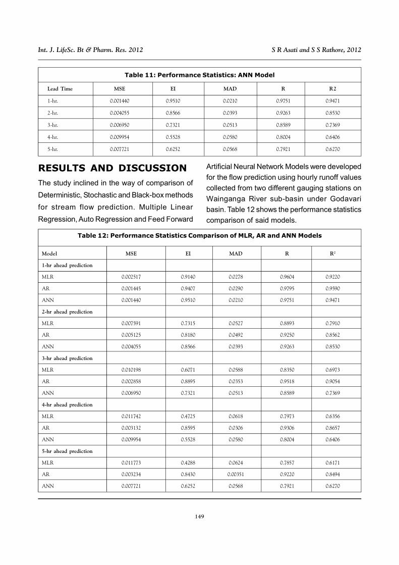
PERFORMANCE STATISTICSTable 11 shows performance statistics of ANNs

models for different lead-time prediction. From

the table, it is found that the value of MSE and

MAD increases while Efficiency Index and

coefficient of correlation decreases with increase

in lead-time prediction.

149


Table 11: Performance Statistics: ANN Model


1-hr. 0.001440 0.9510 0.0210 0.9751 0.9471

2-hr. 0.004055 0.8566 0.0393 0.9263 0.8530

3-hr. 0.006950 0.7321 0.0513 0.8589 0.7369

4-hr. 0.009954 0.5528 0.0580 0.8004 0.6406

5-hr. 0.007721 0.6252 0.0568 0.7921 0.6270

RESULTS AND DISCUSSIONThe study inclined in the way of comparison of

Deterministic, Stochastic and Black-box methods

for stream flow prediction. Multiple Linear

Regression, Auto Regression and Feed Forward

Artificial Neural Network Models were developed

for the flow prediction using hourly runoff values

collected from two different gauging stations on

Wainganga River sub-basin under Godavari

basin. Table 12 shows the performance statistics

comparison of said models.

Model MSE EI MAD R R2

1-hr ahead prediction

MLR 0.002517 0.9140 0.0278 0.9604 0.9220

AR 0.001445 0.9407 0.0290 0.9795 0.9590

ANN 0.001440 0.9510 0.0210 0.9751 0.9471


MLR 0.007591 0.7315 0.0527 0.8893 0.7910

AR 0.005125 0.8180 0.0492 0.9250 0.8562

ANN 0.004055 0.8566 0.0393 0.9263 0.8530


MLR 0.010198 0.6071 0.0588 0.8350 0.6973

AR 0.002858 0.8895 0.0353 0.9518 0.9054

ANN 0.006950 0.7321 0.0513 0.8589 0.7369


MLR 0.011742 0.4725 0.0618 0.7973 0.6356

AR 0.003132 0.8595 0.0306 0.9306 0.8657

ANN 0.009954 0.5528 0.0580 0.8004 0.6406


MLR 0.011773 0.4288 0.0624 0.7857 0.6171

AR 0.003234 0.8430 0.00351 0.9220 0.8494

ANN 0.007721 0.6252 0.0568 0.7921 0.6270

Table 12: Performance Statistics Comparison of MLR, AR and ANN Models

150


CONCLUSIONOne to five hours ahead prediction of Wainganga

river flow is carried out using MLR, AR and ANN.

After analysis, it is observed that AR Model gave

satisfactory results compared to MR and ANN.

Prediction accuracy decreases as lead-time

increases in all these three models except for

four hour ahead prediction. ANN model is found

to be better in simulation and prediction the flow

characteristics under consideration compared to

MLR and AR models for one hour ahead

prediction. However, AR models produce better

predicting results compared to MLR and ANN.

With rigorous exercise on different aspects such

as selection of an appropriate transfer function

best suit to the data, number of hidden layers,

number of neurons in each hidden layers, number

of epochs, ANN models can lead to much better

prediction.

REFERENCES1. A W Minns and M J Hall (1996), “Artificial

Neural Networks as Rainfall Runoff Models,”

Journal Hydrological Sciences, Vol. 41, No.

3, pp. 399-417.

2. Anaund Killingtveit and Nils Roar Saelthun

(1995), “Hydrology,” Norwegian Institute of

Technology, Division of Hydraulic

Engineering, Vol. 7.

3. Asati S R and Rathore S S (2004), “Rainfall

Modelling Using A.N.N.: A case study,”

Proceedings in Hydro- 2004, V.N.I.T.,

Nagpur (M.S.)

4. Asati S R and Rathore S S (2007), “An

Overview on Stream Flow Prediction,”

Proceedings in National Seminar, Ujjain

Engineering College, Ujjain (M.P.).

5. Asati S R and Rathore S S (2007),

“Comparative Study of Stream Flow Models,”

Proceedings in National Conference,

University College of Engineering (A),

Osmania University, Hyderabad.

6. Asati S R and Rathore S S (2008), “Floods

in Gondia Districts: Causes,” Proceedings

in National Conference, B.I.T., Bhilai (C.G.).

7. ASCE Task Committee (2000), “ANN in

Hydrology-I Preliminary Concepts & II

(Hydrologic Applications),” Journal of

Hydrologic Engineering, Vol. 02, pp. 115-

137.

8. Charles T Haan (1995), “Statistical Methods

in Hydrology,” Affiliated East-West Press

Pvt. Ltd., New Delhi.

9. D Achela, K Fernando and A V Jayawerdena

(1998), “Runoff Forecasting Using RBF

Networks with OLS Algorithm”, Journal of

Hydrologic Engg, Vol. 3, pp. 203-209.

10. Dawson C W and Wilby R L (2001),

“Hydrological Modelling Using Artificial Neural

Network,” Progress in physical Geography,

Vol.25, pp.80-108.

11. Dolling O R and Edurardo A V (2002),

“Artificial Neural Networks For Stream Flow

Prediction”, Journal of Hydraulic Research,

Vol. 40, No. 50, pp. 547-554.

12. Gorantiwar S D and Majumdar M (1992),

“Time Series Analysis of Annual Runoff &

Barkar River”, Journal of India Water

Resources Society, Vol. 2, No. 1&2, pp. 117-

121.

13. H Kerem Gigizoglu and Murat Alp (2004),

“Rainfall Runoff Modeling Using Three

Neural Network Methods,” L. Rutkowski et

al (Eds.) ICAISC, pp. 166-171.

14. Huang W, Bing Xu B, and Hiton A (2004),

151


“Forecasting Flows in Apalachicola RiverUsing Neural Networks”, HydrologicalProcesses, 18, pp. 2545-2564.

15. Imric C E, Durcan S and Korre A (2000),“River Flow Prediction Using ANNs:Generalization beyond the CalibrationRange”, Journal of Hydrology, Vol. 233, pp.138-153.

16. Kachroo R K (1992), “River FlowForecasting Part-I-A discussion on thePrinciples,” Journal of Hydrology ElsevierScience, P.B.V., No. 133, pp. 01-15.

17. Karunanithi N, Grenney W J, Whistley D andBovee K (1994), “Neural Network For RiverFlow Prediction”, Journal of Computing inCivil Engineering, ASCE, Vol. 8, No. 2, pp.201-209.

18. Kitadinis P K and Bras R L (1980, a&b),“Real time Forecasting with a ConceptualHydrological Model-Analysis of Uncertainty,”Water Resources Research, Vol. 16, No.6, pp. 1025-1044.

19. M Zakermoshfegh, M Ghodsian and Gh AMontazer (2004), “River Flow ForecastingUsing A NN”, Hydraulics of Dams & Riverstructures -Yazdandoost & Attari (eds.) pp.425–430.

20. Markus M, Salas, J D and Shin H K (1995),“Predicting Stream Flows based on NeuralNetworks”, Proceedings of the 1st

International Conference on WaterResources Engineering, ASCE, New York,pp. 1641-1646.

21. Mutreja K N, Yin A and Martino I (1987),“Flood Forecasting Model for Citandy River”,Flood Hydrology, V.P. Singh, Ed. Reidel,Dordrecht, the Netherlands, pp. 211-220.

22. Nilsson P, Cintia B O and Berndtsson R(2006), “Monthly Runoff Simulation:

Comparing &7 Combining Conceptual &N eural N etw ork M odels”, Journal ofHydrology, Vol.321, pp. 344-363.

23. Raman H and Sunil Kumar N (1995),“Multivariate Modeling of Water ResourcesTime Series Using ANNs”, Journal ofHydrological Sciences, Vol. 40, pp. 145-163.

24. Sarkar A, Agrawal A and Singh R D (2006),“ANNs Models For Rainfall RunoffForecasting in a Hilly Catchments”, Journalof Indian water Resources Society, Vol. 26,No. 3-4, pp. 5-12.

25. Smith J & Eli R.N (1995), “Neural NetworkModels for Rainfall Runoff Process,” Journalof Water Resources Planning &Management, ASCE, Vol. 121, No.6, pp.499-508.

26. Srinivasula S and Jain Ashu (2009), “RiverFlow Prediction Using an IntegratedApproach”, Journal of HydrologicEngineering © ASCE, pp. 75-83.

27. Thirumalaih K and Deo M C (2000),“Hydrological Forecasting Using NeuralNetworks”, Journal of HydrologicEngineering, ASCE, pp. 180-189.

28. Thomas T, Jaiswal R K, Galkate Ravi andSurjeet Singh (2009): “Artificial NeuralNetworks Modeling on Stream Flows forSindh Basin in Madhya Pradesh”, Journalof Indian Water Resources Society, Vol. 29,No.1, pp.08-16.

29. Weeks W Daa et al., (1987), “Tests of ARMAModel for Rainfall Runoff Modelling”, Journalof Hydrology Elsevier Science, Pub. B.V.,pp. 01-15.

30. Zealand C, Burn D, Simonovic S (1999):“Short Term Stream Flow Forecasting UsingArtificial Neural Networks”, Journal of

Hydrology, 214, pp. 32-48.

COMPARATIVE STUDY OF STREAM FLOW PREDICTION MODELS … · COMPARATIVE STUDY OF STREAM FLOW...

Documents

Transcript of COMPARATIVE STUDY OF STREAM FLOW PREDICTION MODELS … · COMPARATIVE STUDY OF STREAM FLOW...