Mixed-Effect Models for Prediction of Tree...
92
Mixed-effects models prediction Mixed-Effect Models for Prediction of Tree Attributes Lauri Mehtätalo 1 1 University of Eastern Finland, School of Computing III Brazilian Mensurationist Meeting Piracicaba, Sao Paulo August 18, 2016 Mehtätalo Mixed-effects models prediction
Transcript of Mixed-Effect Models for Prediction of Tree...

Mixed-effects models prediction
Mixed-Effect Models for Prediction of Tree Attributes
Lauri Mehtätalo1
1University of Eastern Finland, School of Computing
III Brazilian Mensurationist MeetingPiracicaba, Sao Paulo
August 18, 2016
Mehtätalo Mixed-effects models prediction

Mixed-effects models prediction
Outline
1 Introduction
2 Single-level LME with random constantModel formulationParameter estimationA fixed-effects modelExample 1: Eucalyptus volume
3 Mode advanced mixed-effects modelsModel formulationPrediction of random effects
4 2 more examplesExample 2: a model for H-D relationshipExample 3: Eucalyptus volumes on two rotations
5 Discussion and conclusions
Mehtätalo Mixed-effects models prediction

Mixed-effects models prediction
Introduction
Types of forest datasets
Forest datasets are usually grouped e.g.needles within branches,branches within trees,trees within sample plots or aerial images,sample plots within forest stands,forest stand within regionsrepeated observations of trees (e.g., in successive years or on different images)...
A dataset may also have multiple nested or grouped levelsRepeated measurements of trees within sample plots (nested)Tree increments for different calendar years (crossed)
These groups often constitute a sample from a population of groups, and aretherefore naturally modeled using mixed-effect models.
Mehtätalo Mixed-effects models prediction

Mixed-effects models prediction
Single-level LME with random constant
Model formulation
Linear mixed-effect model with random constant
yij = β′x ij + bi + εij ,
where
yij is the observed response for individual j in group i ,
x ij is a vector of fixed predictors,
β includes the fixed parameters,
bi are random group effects for groups i = 1, . . . ,M.
We assume bi ∼ N(0, σ2b) (i.i.d); εij ∼ N(0, σ2) (i.i.d); bi are independent of εij .
Model parameters are β, σ2b , and σ2. Also group effects bi can be predicted.
Can be seen as a marginal model yij = β′x ij + eij , where var(yij ) = σ2b + σ2
and cov(yij , yij′) = σ2b .
Mehtätalo Mixed-effects models prediction

Mixed-effects models prediction
Single-level LME with random constant
Parameter estimation
Parameter estimation
The (restricted) likelihood for the marginal model yij = β′x ij + eij is easy to writeto get (RE)ML estimates of parameters σ2
b and σ2, and GLS/REML/ML estimatesof β.
The random group effects can be predicted using Best Linear UnbiasedPredictor (BLUP)
bi =σ2
b1niσ2 + σ2
b
(yi − ¯β′x ij )
where yi and ¯β′x ij are the means of the ni observed values and fixed-partpredictions for the group in question.
The prediction variance is
var
(bi − bi
)=
(σ2
b1niσ2 + σ2
b
)σ2
ni
In practice, we use Empirical BLUP where the unknown β, σ2b and σ2 are
replaced by their numerical estimates.
Mehtätalo Mixed-effects models prediction

Mixed-effects models prediction
Single-level LME with random constant
A fixed-effects model
A corresponding model with fixed group effects
Consider an otherwise similar model
yij = β′x ij + bi + εij ,
where
bi are fixed group effects for groups i = 1, . . . ,M.
Model parameters are β, σ2, and bi for i = 1, . . . ,M.
Identifiable only if β′x ij does not include a constant term.
The estimate of group effect is
bi = yi − ¯β′x ij
The variance is
var
(bi − bi
)=σ2
ni.
Mehtätalo Mixed-effects models prediction

Mixed-effects models prediction
Single-level LME with random constant
A fixed-effects model
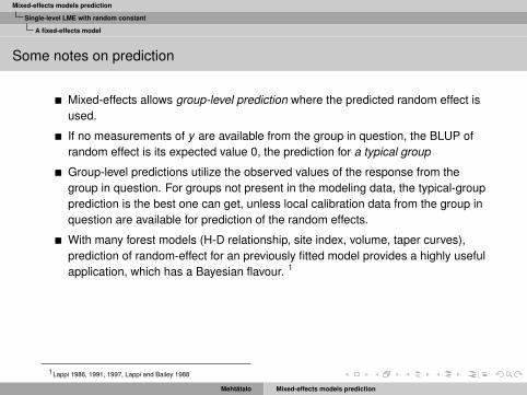
Some notes on prediction
Mixed-effects allows group-level prediction where the predicted random effect isused.
If no measurements of y are available from the group in question, the BLUP ofrandom effect is its expected value 0, the prediction for a typical group
Group-level predictions utilize the observed values of the response from thegroup in question. For groups not present in the modeling data, the typical-groupprediction is the best one can get, unless local calibration data from the group inquestion are available for prediction of the random effects.
With many forest models (H-D relationship, site index, volume, taper curves),prediction of random-effect for an previously fitted model provides a highly usefulapplication, which has a Bayesian flavour. 1
The BLUP of random effects is only marginally unbiased but conditionallybiased. The fixed group effect is also conditionally unbiased.
For a well-formulated linear mixed-effects model, the fixed part has also theinterpretation as the marginal prediction over groups.
1Lappi 1986, 1991, 1997, Lappi and Bailey 1988
Mehtätalo Mixed-effects models prediction

Mixed-effects models prediction
Single-level LME with random constant
A fixed-effects model
Some notes on prediction
Mixed-effects allows group-level prediction where the predicted random effect isused.
If no measurements of y are available from the group in question, the BLUP ofrandom effect is its expected value 0, the prediction for a typical group
Group-level predictions utilize the observed values of the response from thegroup in question. For groups not present in the modeling data, the typical-groupprediction is the best one can get, unless local calibration data from the group inquestion are available for prediction of the random effects.
With many forest models (H-D relationship, site index, volume, taper curves),prediction of random-effect for an previously fitted model provides a highly usefulapplication, which has a Bayesian flavour. 1
The BLUP of random effects is only marginally unbiased but conditionallybiased. The fixed group effect is also conditionally unbiased.
For a well-formulated linear mixed-effects model, the fixed part has also theinterpretation as the marginal prediction over groups.
1Lappi 1986, 1991, 1997, Lappi and Bailey 1988
Mehtätalo Mixed-effects models prediction

Mixed-effects models prediction
Single-level LME with random constant
Example 1: Eucalyptus volume
Example 1: Volume of eucalyptus trees
Modelln(vij ) = β0 + β1 ln(dbhij ) + β2 ln(hij ) + bi + εij
was fitted for the volume of Eucalyptus trees j on farms i , using a stem analysis dataof 1434 stems from 15 farms 2.The parameter estimates for random part were σ2
b = 0.182 and σ2 = 0.622.Therefore, some benefit may be obtained by prediction of random effects, as shownbelow.
2de Souza Vismara et al. 2016Mehtätalo Mixed-effects models prediction

Mixed-effects models prediction
Mode advanced mixed-effects models
Model formulation
More advanced mixed-effects models
One may have other random effects than just constant:
yij = β′x ij + b′i z ij + εij
where z ij includes x ij or part of it, and bi ∼ N(0,D) (i.i.d).
For two nested groups, we specify
yijk = β′x ijk + a′i z(a)ijk + c′ij z
(c)ijk + εijk
where z(a)ijk includes x ijk or part of it, and z(c)
ijk includes z(a)ijk or part of it, and
ai ∼ N(0,Da) (i.i.d) and cij ∼ N(0,Dc) (i.i.d).
Mehtätalo Mixed-effects models prediction

Mixed-effects models prediction
Mode advanced mixed-effects models
Model formulation
More advanced mixed-effects models
For two crossed groups 3, we specify
yijk = β′x ijk + a′i z(a)ijk + c′j z
(c)ijk + εijk
where z(a)ijk and z(c)
ijk includes x ijk or part of it and ai ∼ N(0,Da) (i.i.d) andcj ∼ N(0,Dc) (i.i.d).
A bivariate LMM (with single level of grouping) may be specified by 4
y1ij = β′x1ij + b1′i z1ij + ε1ij
y2ij = β′x2ij + b2′i z2ij + ε2ij
where (b1′k , b2′i )′ ∼ N(0,D) (iid) and (ε1k , ε2k )′ ∼ N(0,R).
The assumption of constant error variance can also be relaxed using variancefunctions/ correlation structures.
Parameter estimation can be based on (RE)ML/GLS.
Prediction of random effect is based on the general formulation of BLUP.
3e.g. Mehtätalo et al 2014, Korpela et al. 20144e.g. Lappi 1991, Mehtätalo 2005, Lappi et al. 2006, Maltamo et al 2012. Korpela et al 2014
Mehtätalo Mixed-effects models prediction

Mixed-effects models prediction
Mode advanced mixed-effects models
Model formulation
More advanced mixed-effects models
For two crossed groups 3, we specify
yijk = β′x ijk + a′i z(a)ijk + c′j z
(c)ijk + εijk
where z(a)ijk and z(c)
ijk includes x ijk or part of it and ai ∼ N(0,Da) (i.i.d) andcj ∼ N(0,Dc) (i.i.d).
A bivariate LMM (with single level of grouping) may be specified by 4
y1ij = β′x1ij + b1′i z1ij + ε1ij
y2ij = β′x2ij + b2′i z2ij + ε2ij
where (b1′k , b2′i )′ ∼ N(0,D) (iid) and (ε1k , ε2k )′ ∼ N(0,R).
The assumption of constant error variance can also be relaxed using variancefunctions/ correlation structures.
Parameter estimation can be based on (RE)ML/GLS.
Prediction of random effect is based on the general formulation of BLUP.3e.g. Mehtätalo et al 2014, Korpela et al. 20144e.g. Lappi 1991, Mehtätalo 2005, Lappi et al. 2006, Maltamo et al 2012. Korpela et al 2014
Mehtätalo Mixed-effects models prediction

Mixed-effects models prediction
Mode advanced mixed-effects models
Prediction of random effects
BLUP - the general case
Consider random vector h which is partitioned as follows:
h =
(h1
h2
)and has the following mean and variance:(
h1
h2
)∼[(
µ1
µ2
),
(V1 V12
V′12 V2
)]Consider a situation where the value of h2 has been observed and one wants topredict the value of unobserved vector h1.The Best Linear Unbiased Predictor (BLUP) of h1 is
BLUP(h1) = h1 = µ1 + V12V−12 (h2 − µ2) (1)
The prediction variance is
var(h1 − h1) = V1 − V12V−12 V′12 (2)
If h has multivariate normal distribution, BLUP is BP.If the mean and variances are estimates, the resulting estimator is calledEstimated or empirical BLUP (EBLUP).
Mehtätalo Mixed-effects models prediction

Mixed-effects models prediction
2 more examples
Example 2: a model for H-D relationship
Example 2: A longitudinal H-D model
H-D relationship varies much amongsample plots, but heightmeasurement is time-consuming.
In a forest inventory, diameter isusually tallied for all trees of a sampleplot, whereas height is measuredonly for 0 – 5 trees per plot.
●
●
●
●
●●
●
●
●
●
●
●
●
●
●
●
●
●
●
●
●
●
●
●
●
●
●
●
●
●
●
●
●
●
●
●
●
●●
●
●
●
●
●
●
●
●
●
●
●
●
●
●
●
●
●
●
●
●
●
●
●
●●
●
●
●
●
●
●
●
●
●
●
●
●
●
●
●
●
●
●●
●
●
●
●
●
●
●
●
●●
●
●
●
●
●
●
●
●
●
●
●
●
●
●
●
●
●
●
●
●
●
●
●
●
●
●
●
●
●
●
●
●
●
●
●
●
●
●
●
●
●
●
●
●
●
●
●
●
●
●
●
●
●
●
●
●
●●
●
●
●
●
●
●
●
●
●
●
●
●
●
●
●
●
●
●
●
●
●
●
●
●
●
●
●
●
●
●
●
●
●
●
●
●
●
●
●
●●
●
●
●
●
●
●
●
●
●
●
●
●
●●
●
●
●
●
●
●
●
●
●
●
●
●
●
●
●
●
●
●
●
●
●
●
●
●
●
●
●
●
●
●
●
●
●
●
●
●
●
●
●●
●
●
●
●
●
●
●
●
●
●
●
●
●
●
●
●
●
●
●
●
●
●
●
●
●
●
●●
●
●
●
●
●
●
●
●
●
●
●
●
●
●
●
●
●
●
●
●
●
●
●
●
●
●
●
●
●
●
●
●●
●
●
●
●
●
●
●
●
●
●
●●
●
●
●
●
●
●
●●
●●
●
●●
●
●
●
●
●
●
●
●
●
●
●
●
●
●
●
●
●
●
●●
●
●
●
●
●
●
●
●
●
●●
●
●
●
●
●
●
●
●
●
●
●
●
●
●
●
●
●
●●
●
●
●
●
●
●
●
●
●
●
●
●
●
●
●
●
●
●
●
●
●
●
●
●
●
●
●
●
●
●
●
●
●
●
●
●
●
●
●
●
●
●
●
●
●
●
●
●
●
●
●
●●
●
●
●
●
●●
●
●
●
●
●
●
●
●
●
●
●
●
●
●
●
●
●
●
●
●
●
●
●
●●
●
●
●
●
●●
●
●
●
●
●
●
●
●
●
●
●
●
●●
●
●
●
●
●
●●
●
●
●
●
●
●●
●
●
●
●
●
●
●
●
●
●
●
●
●
●
●
●
●
●
●
●
●
●
●
●
●
●
●
●
●
●
●
●
●
●
●●
●
●
●
●
●
●
●
●
●
●
●
●
●
●
●
●
●
●
●
●
●
●
●
●
●●
●
●
●
●
●
●
●●
●●
●
●
●
●●
●
●
●
●
●
●
●
●●
●
●●●
●
●
●
●
●
●●
●
●
●
●●
●●●
●
●
●
●
●
●
●
●●
●
●
●●
●
●
●
●
●
●
●
●
●
●
●●
●
●●
●
●
●
●
●
●
●
●
●
●
●
●
●
●
●
●
●
●
●
●●
●
●
●
●
●
●
●
●
●
●
●
●
●
●
●
●
●
●
●
●
●
●
●
●●
●
●
●
●
●
●
●
●
●
●
●
●
●●
●
●
●
●
●
●●
●
●
●
●
●
●
●
●
●
●
●
●
●
●
●●
●
●
●
●
●
●
●
●
●
●●
●
●
●
●
●●
● ●
●
●●
●
●
●
●
●
●
●
●
●
●
●
●●
●
●
●
●
●
●
●
●●
●
●
●
●
●
●
●
●
●
●
●●
●
●●
●
●●
●
●
●
●
●
●
●
●
●
●
●●
●
●
●
●
●
●●
●
●
●
●
●
●
●●
●
●
●
●
●
●
●
●
●
●
●
●
●
●●
●
●
●
●
●
●
●
●
●
●●
●
●
●
●
●
●●
●
●
●
●
●●
●●●
●
●
●
●●
●
●●
●●
●
● ●
●●
●
●
●
●
●
●
●
●
●
●
●
●
●
●
●
●
●
●
●
●
●
●
●
●
●
●
●
●
●●
●●
●
●
●
●
●
●
●
●
●
●
●
●
●
●
●
●
●
●
●
●
●
●
●
●
●
●
●
●
●
●
●
●
●
●
●
●●
●
●
●
●●●
●
●
●
●
●
●
●
●
●
● ●
●
●
●
●
●
●●
●
●
●
●
●
●●
●
●
●
●
●
●
●●
●
●
●
●
●
●●
●
●
●
●
●
●
●
●
●
●
●
●
●●
●
●●●
●
●
●
●●
●
●
●●
●
●●
●●
●
●●
●
●
●
●
●
●
●
●
●●
●●
●
●
●
●
●
●●
●
●
●
●●
●
●
●
●
●
●
●
●
●
●
●
●
●
●
●
●
●●
●●
●
●
●
●
●
●
●
●
●
●
●
●
●
●
●
●
●
●
●
●
●
●
●
●
●
●
●●●
●
●
●
●
●
●●
●●●
●
●
●
●
●●
●
●
●
●
●
●
●
●
●
●
●
●●
●
●
●
●
●●
●
●
●
●
●
●
●
●
●●●
●
●
●
●
●
●
●
●
●●
●
●●
●
●
●
●
●
●
●
●
●
●
●●●
●
●
●
●●
●
●
●
●
●
●
●
●
●
●
●●
●
●
●
●
●●
●●
●
●●
●●
●
●
●
●
●
●
●
●
●
●
●
●
●●
●
●
●
●
●
●
●
●
●
●
●
●
●
●
●●
●
●
● ●●●
●
●●
●
●
●
●
●
●
●●
●
●
●
●
●
●
●
●
●●
●●
●
●●
●
●
●
●
●
●
●●
●
●
●●
●
●
●
●
●
●
●
●
●
●
●
●
●
●
●
●
●●
●
●
●
●
●
●
●
●
●
●
●
●
●
●
●
●
●
●
●
●
●
●
●
●
●
●
●
●
●●
●
●
●
●
●
●
●
●
●
●
●
●
●
●
●●
●●
●
●
●
●
●
●
●
●●
●●
●
●
●
●
●
●
●
●
●
●
●
●
●
●●
●
●
●●
●
●
●●
●●●●
●●●
●
●●
●
●
●
●
●
●
●
●
●●
●
●
●
●
●
●
●
●
●
●
●
●
●
●●
●
●
●
●●
●
●
●
●
●
●
●
●
●
●
●
●●
●
●
●
●●
●
●
●
●
●
●
●
●
●
●
●
●
●
●
●
●
●
●
●
●
●
●●
●
●
●
●
●
●
●
●
●
●
●
●
●
●
●
●
●
●
●
●
●
●
●●●
●●
●
●
●
●
●
●
●
●
●
●
●● ●
●
●
●●
●
●
●
●
●
●
● ●
●
●
●
●●
●
●
●
●●
● ●
●
●●
●
●
●
●
●
●
●
●
●
●
●●
●
●
●
●
●
●
●
●
●
●
●
●
●
●
●
●
●
●
●
●
●
●
●
●
●
●
●●
●
●
●
●
●
●
●●
●
●
●
●
●
●
●
●
●
●
●
●
●
●
●●●
●
●
●
●
●
●
●●
●●
●
●
●
●
●
●
●
●
●
●●●
●
●
●
●
●
●
●●
●
●
●
●
●
●
●
●
●
●
●
●
●●
●
●●
●
●
●
●
●
●
●●
●
●
●
●
●
●
●
●
●●
●
●
●
●
●●
●●● ●
●●
●
●●
●●
●
●
●
●●
●
●
●●
●
●
●
●
●
●
●
●●
●
●
●
●
0 10 20 30 40 500
510
1520
2530
Tree height vs Tree diameter
d, cm
h, m
If a previously fitted H-D model is available, it can be localized, or calibrated, for thenew plot by predicting the random effects using the sampled tree heights.
Mehtätalo Mixed-effects models prediction

Mixed-effects models prediction
2 more examples
Example 2: a model for H-D relationship
The Height-Diameter model
The logarithmic heigth Hijk for tree k in stand i at time j with transformed diameter Dijk
at the breast height is expressed by 5
ln(Hijk ) = β0(DGMij ) + a(1)i + c(1)
ij + (β1(DGMkt ) + a(2)i + c(2)
ij )Dijk + εijk
= β0(DGMij ) + β1(DGMkt )Dijk + a(1)i + a(2)
i Dijk + c(1)ij + c(2)
ij Dijk + εijk ,
where
β0(DGMij ) and β1(DGMij ) are known fixed functions of plot-specific meandiameter DGMij ,
a = (a(1)i , a(2)
i )′ are plot-level random effects
c = (c(1)ij , c
(2)ij )′ are measurement occasion -level random effects
The variances (correlations) were estimated to be
var(ai ) =
[0.1082 (0.269)0.0028 0.09582
]var(cij ) =
[0.01682 (−0.681)−0.0003 0.02232
]εijk are independent normal residuals withvar(εijk ) = 0.4012
(max(Dijk , 7.5)
)−1.068
5Mehtätalo 2004, 2005
Mehtätalo Mixed-effects models prediction

Mixed-effects models prediction
2 more examples
Example 2: a model for H-D relationship
The Height-Diameter model
The logarithmic heigth Hijk for tree k in stand i at time j with transformed diameter Dijk
at the breast height is expressed by 5
ln(Hijk ) = β0(DGMij ) + a(1)i + c(1)
ij + (β1(DGMkt ) + a(2)i + c(2)
ij )Dijk + εijk
= β0(DGMij ) + β1(DGMkt )Dijk + a(1)i + a(2)
i Dijk + c(1)ij + c(2)
ij Dijk + εijk ,
where
β0(DGMij ) and β1(DGMij ) are known fixed functions of plot-specific meandiameter DGMij ,
a = (a(1)i , a(2)
i )′ are plot-level random effects
c = (c(1)ij , c
(2)ij )′ are measurement occasion -level random effects
The variances (correlations) were estimated to be
var(ai ) =
[0.1082 (0.269)0.0028 0.09582
]var(cij ) =
[0.01682 (−0.681)−0.0003 0.02232
]
εijk are independent normal residuals withvar(εijk ) = 0.4012
(max(Dijk , 7.5)
)−1.068
5Mehtätalo 2004, 2005
Mehtätalo Mixed-effects models prediction

Mixed-effects models prediction
2 more examples
Example 2: a model for H-D relationship
The Height-Diameter model
The logarithmic heigth Hijk for tree k in stand i at time j with transformed diameter Dijk
at the breast height is expressed by 5
ln(Hijk ) = β0(DGMij ) + a(1)i + c(1)
ij + (β1(DGMkt ) + a(2)i + c(2)
ij )Dijk + εijk
= β0(DGMij ) + β1(DGMkt )Dijk + a(1)i + a(2)
i Dijk + c(1)ij + c(2)
ij Dijk + εijk ,
where
β0(DGMij ) and β1(DGMij ) are known fixed functions of plot-specific meandiameter DGMij ,
a = (a(1)i , a(2)
i )′ are plot-level random effects
c = (c(1)ij , c
(2)ij )′ are measurement occasion -level random effects
The variances (correlations) were estimated to be
var(ai ) =
[0.1082 (0.269)0.0028 0.09582
]var(cij ) =
[0.01682 (−0.681)−0.0003 0.02232
]εijk are independent normal residuals withvar(εijk ) = 0.4012
(max(Dijk , 7.5)
)−1.068
5Mehtätalo 2004, 2005
Mehtätalo Mixed-effects models prediction

Mixed-effects models prediction
2 more examples
Example 2: a model for H-D relationship
The stand level mixed-effects model
The sample tree heights of a new stand i can be described by model
y i = X iβ + Z i bi + εi ,
wherey i includes the observed sample tree heights,X iβ is the fixed part,bi = ( a(1)
i a(2)i c(1)
i1 c(2)i1 c(1)
i2 c(2)i2 . . .)
′includes the random effects,
Z i is the random part design matrix of the group, andεi includes the residuals.We denote var(bi ) = D and var(εi ) = R i .
Mehtätalo Mixed-effects models prediction

Mixed-effects models prediction
2 more examples
Example 2: a model for H-D relationship
Prediction of random effects
The variances and covariances between random effects and observed heights can bewritten as [
bi
y i
]∼
([0
X iβ
],
[D DZ ′i
Z i D Z i DZ ′i + R i
])The Empirical Best Linear Unbiased Predictor (EBLUP) of random effects is
bi = DZ ′i (Z i DZ ′i + R i )−1(y i − X iβ) .
and the variance of prediction errors is
var(bi − bi ) = D − DZ ′i (Z i DZ ′i + R i )−1Z i D
Mehtätalo Mixed-effects models prediction

Mixed-effects models prediction
2 more examples
Example 2: a model for H-D relationship
Example
Height of one tree was measured 5 years ago and 2 trees at the current year. Thematrices and vectors are
µ =
2.592.112.99
y =
2.772.353.19
Z =
1 −0.36 1 −0.36 0 01 −1.22 0 0 1 −1.221 0.058 0 0 1 0.058
R =
0.008 0 00 0.016 00 0 0.004
β =
αk
βk
αk1
βk1
αk2
βk2
D =
0.0118 0.0028 0 0 0 00.0028 0.0092 0 0 0 0
0 0 0.0003 0.0004 0 00 0 0.0004 0.0005 0 00 0 0 0 0.0003 0.00040 0 0 0 0.0004 0.0005
Mehtätalo Mixed-effects models prediction
Mixed-effects models prediction
2 more examples
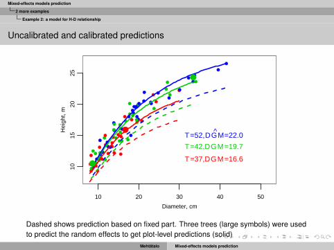
Example 2: a model for H-D relationship
Uncalibrated and calibrated predictions
●
●
●
●
●
●
●
●
●
●
●
●
●
●
●
●
●
●
●
●
●
●
●
●
●
●
●
●
●
●
●
●●
●
●
●
●
●
●
●
●
●●
●
●
●
●
●
●
●
●
●●
●
●
●
●
●
●
●
●
●
●
●
●
●
●
●
●
●
●
●
●●
●
●
●● ●
●
●
●
●
●
●
●
●
●
●●
●
●
10 20 30 40 50
1015
2025
Diameter, cm
Hei
ght,
m
●
●
●
T=52,DGM^ =22.0
T=42,DGM=19.7
T=37,DGM=16.6
Dashed shows prediction based on fixed part. Three trees (large symbols) were usedto predict the random effects to get plot-level predictions (solid)
Mehtätalo Mixed-effects models prediction

Mixed-effects models prediction
2 more examples
Example 3: Eucalyptus volumes on two rotations
Example 3: Eucalyptus volumes on two rotations
A bivariate volume model
ln(v1ij ) = β′1x1ij + b(1)i + ε1ij
ln(v2ij ) = β′2x2ij + b(2)i + ε2ij
was used for rotations 1 and 2 of Eucalyptus plantations 6.The parameter estimates for random part were
var
(b(1)
i
b(2)i
)=
(0.01922 0.0005170176
0.0005170176 0.02722
)=(
C H)
and
var
(ε1ij
ε2ij
)=
(0.0624 0
0 0.05962
)
The correlation between random effects is high (0.99), therefore both models could becalibrated by using observations of first rotation only.The error variance is high compared to that of random effects,→ calibration effectswill be only modest.
6de Souza Vismara, Mehtatalo and Batista 2016
Mehtätalo Mixed-effects models prediction

Mixed-effects models prediction
2 more examples
Example 3: Eucalyptus volumes on two rotations
Example 3: Eucalyptus volumes on two rotations
A bivariate volume model
ln(v1ij ) = β′1x1ij + b(1)i + ε1ij
ln(v2ij ) = β′2x2ij + b(2)i + ε2ij
was used for rotations 1 and 2 of Eucalyptus plantations 6.The parameter estimates for random part were
var
(b(1)
i
b(2)i
)=
(0.01922 0.0005170176
0.0005170176 0.02722
)=(
C H)
and
var
(ε1ij
ε2ij
)=
(0.0624 0
0 0.05962
)The correlation between random effects is high (0.99), therefore both models could becalibrated by using observations of first rotation only.
The error variance is high compared to that of random effects,→ calibration effectswill be only modest.
6de Souza Vismara, Mehtatalo and Batista 2016
Mehtätalo Mixed-effects models prediction

Mixed-effects models prediction
2 more examples
Example 3: Eucalyptus volumes on two rotations
Example 3: Eucalyptus volumes on two rotations
A bivariate volume model
ln(v1ij ) = β′1x1ij + b(1)i + ε1ij
ln(v2ij ) = β′2x2ij + b(2)i + ε2ij
was used for rotations 1 and 2 of Eucalyptus plantations 6.The parameter estimates for random part were
var
(b(1)
i
b(2)i
)=
(0.01922 0.0005170176
0.0005170176 0.02722
)=(
C H)
and
var
(ε1ij
ε2ij
)=
(0.0624 0
0 0.05962
)The correlation between random effects is high (0.99), therefore both models could becalibrated by using observations of first rotation only.The error variance is high compared to that of random effects,→ calibration effectswill be only modest.
6de Souza Vismara, Mehtatalo and Batista 2016
Mehtätalo Mixed-effects models prediction

Mixed-effects models prediction
2 more examples
Example 3: Eucalyptus volumes on two rotations
BLUP in this case
We have now[bi
ln v1i
]∼
([0
X 1iβ1
],
[D CZ ′1i
Z 1i C′ Z 1ivar(b(1)i )Z ′1i + R1i
])Leading to EBLUP:
bi = CZ ′1i
(Z 1ivar(b(1)
i )Z ′1i + R1i
)−1(ln v1i − X 1iβ1) .
etc..
Figure : The RMSE and ME of second-rotation trees as a function of first-rotation sample trees.Mehtätalo Mixed-effects models prediction

Mixed-effects models prediction
Discussion and conclusions
Discussion and conclusions
Random-effect prediction is a widely applicable tool for many different situationsbeyond mixed-effect models and beyond the standard implementations instatistical software. For example, linear regression and kriging are applications ofthe general form BLUP.Random effects may be justified for many different purposes, and modelingprocedures should be adopted for the purpose of modeling.
local predictions through random effects.statistical inference in grouped datasetsvariance partitioning
I do not see (m)any reasons to treat group effects as fixed if not all groups of thepopulation are not represented by the data.
Mehtätalo Mixed-effects models prediction

Mixed-effects models prediction
Discussion and conclusions
References
de Souza Vismara, E., Mehtätalo, L., and Batista, J.L.F. 2016. Linear mixed-effects models and calibration applied tovolume models in two rotations of Eucalyptus grandis plantations. Can. J. For. Res. 46(1): 132-141
Korpela, I., Mehtätalo, L., Markelin, L., Seppänen, A. and Kangas, A. 2014.Tree species identification in aerial image datausing directional reflectance signatures. Silva Fenn. 48(3): 1087
Lappi, J. 1986. Mixed linear models for analyzing and predicting stem form variation of Scots pine. CommunicationesInstituti Forestalis Fenniae 134. 69 p.
Lappi, J. and Bailey, R. L. 1988. A height prediction model with random stand and tree parameters: an alternative totraditional site index methods. For. Sci 34: 907–927.
Lappi, J. 1991. Calibration of height and volume equations with random parameters. For. Sci. 37(3): 781-801.
Lappi, J. 1997. A longitudinal analysis of height/diameter curves. For. Sci. 43. 555–570.
Lappi, J., Mehtätalo, L. and Korhonen, K.T. 2006. Generalizing sample tree information. in Kangas, A. and Maltamo, M(editors) Forest inventory - methodology & applications. Springer.
Mehtätalo, L. 2004. A longitudinal height-diameter model for Norway spruce in Finland. Can. J. For. Res. 34(1): 131-140.
Mehtätalo, L. 2005a. Height-diameter models for Scots pine and birch in Finland. Silva Fennica 39(1): 55-66.
Mehtätalo, L. 2005b. Localizing a Predicted Diameter Distribution Using Sample Information For. Sci. 51(4):292U303.
Mehtätalo, L., Peltola, H., Kilpeläinen, A. and Ikonen, V.-P. 2014. The effect of thinning on the basal area growth of ScotsPine: a longitudinal analysis using nonlinear mixed-effects model. For.Sci. 60(4):636-644
Maltamo, M., Mehtätalo, L., Vauhkonen, J. and Packalén P. 2012. Predicting and calibrating tree attributes by means ofairborne laser scanning and field measurements. Can. J. For. Res. 42: 1896-1907
Mehtätalo Mixed-effects models prediction

Mixed-effects models prediction
Case 2: Extracting effects of silviculturalthinnings
Utilizing a prediction from a linear mixed-effectsmodel with crossed tree and calendar year effects
Mehtätalo, L., Peltola, H., Kilpeläinen, A. and Ikonen, V.-P. 2013. The effect of thinningon the basal area growth of Scots Pine: a longitudinal analysis using nonlinearmixed-effects model. Submitted manuscript.
Mehtätalo Mixed-effects models prediction

Mixed-effects models prediction
Extracting thinning effects
Why thinning effects?
Forest managers use silvicultural thinnings to decrease the competition ofneighboring trees and, consequently, to increase the growth rate of theremaining trees for faster production of sawtimber.
To understand the dynamics of thinning, one may wish to analyse the effect ofthinnings on tree growth.
However, the growth is affected also by other factors, especially by the siteproductivity, tree age, and annual weather.
Mixed-effects models can be used to model out these nuisance effects.
Mehtätalo Mixed-effects models prediction

Mixed-effects models prediction
Extracting thinning effects
Study material
Thinning experiment sample plots were established in naturally generated Scotspine stands at the age of ∼ 25 years in Mekrijärvi, Finland in 1986.
One of the four following thinning treatments were applied to each plot: Nothinning (I, Control), light (II), moderate (III), and heavy (IV) thinnings.
88 trees were felled in 2006, and the complete time series of diameterincrements between 1983 and 2006 was measured for each tree using an X-raydensiometer.
The diameter growths were transformed to basal area growths, becauseVolume ∼ Diameter 2Height)
Mehtätalo Mixed-effects models prediction

Mixed-effects models prediction
Extracting thinning effects
The raw data
1985 1990 1995 2000 2005
020
040
060
080
010
00
Year
Rin
g B
asal
are
a, m
m2
I (control) - black; II (light) - redIII (moderate) - green; IV (heavy) - blue
THICK: treatment-specific trends
THIN: 12 randomly selected trees
One can see
(Age trend)climate-related year effectstree effects
Mehtätalo Mixed-effects models prediction

Mixed-effects models prediction
Extracting thinning effects
Modeling the non-thinned response
A dataset without thinning treatments was produced by including from theoriginal data
The control treatment for whole follow-up periodThe thinned treatments until the year of thinning (1986)
A linear mixed effect model with random year and tree effects was fitted to theunthinned data
ykt = f (Tkt ; b) + αk + αt + εkt (3)
where ykt is the basal area growth of tree k at year t ,f (Tkt ; b) is the age trend (modeled using a spline),αk is a NID tree effect,αt is a NID year effect andεkt is a NID residual.
Mehtätalo Mixed-effects models prediction

Mixed-effects models prediction
Extracting thinning effects
Extracting the thinning effects
Using the estimated age trend and BLUP’s of year and tree effects, the growthwithout thinning, ykt was predicted for treatments II -IV after the thinning year.
The pure thinning effects were estimated by subtracting the prediction from theobserved growth
dkt = ykt − ykt (4)
Mehtätalo Mixed-effects models prediction

Mixed-effects models prediction
Extracting thinning effects
Extracting the thinning effects
Using the estimated age trend and BLUP’s of year and tree effects, the growthwithout thinning, ykt was predicted for treatments II -IV after the thinning year.The pure thinning effects were estimated by subtracting the prediction from theobserved growth
dkt = ykt − ykt (4)
Mehtätalo Mixed-effects models prediction

Mixed-effects models prediction
Extracting thinning effects
The estimated thinning effects
Extracted thinning effects
1985 1990 1995 2000 2005
−20
00
200
400
600
Year
Thi
nnin
g ef
fect
of R
ing
Bas
al A
rea
Raw data
1985 1990 1995 2000 2005
020
040
060
080
010
00
Year
Rin
g B
asal
are
a, m
m2
Line color specifies treatment (I:black, II: red, III: green IV: blue). Thick lines show thetreatment-specific mean trends; thin lines show 12 randomly selected trees.
Mehtätalo Mixed-effects models prediction

Mixed-effects models prediction
Modeling thinning effects using NLME’s
Case 3: Modelling thinning effects usingNLME’s
A nonlinear model to analyze the effect of thinningintensity and tree size on the dynamics of tree-level
thinning effect.Mehtätalo, L., Peltola, H., Kilpeläinen, A. and Ikonen, V.-P. 2013. The effect of thinningon the basal area growth of Scots Pine: a longitudinal analysis using nonlinearmixed-effects model. Submitted manuscript.
Mehtätalo Mixed-effects models prediction

Mixed-effects models prediction
Modeling thinning effects using NLME’s
Modeling the thinning effects
The thinning effects seem to switch on during a short time called Reaction timeand stabilize thereafter at a level of Maximum thinning effect.
To explore what predictors control these two parameters, the thinning effects ofthe thinnend treatments 2-4 were modeled using a nonlinear mixed-effectsmodel.
The random effects were used to take into account the data hierarchy for morereliable inference.
Mehtätalo Mixed-effects models prediction

Mixed-effects models prediction
Modeling thinning effects using NLME’s
Nonlinear mixed-effects model for thinning effect
The thinning effect of tree k at time t was modeled using a logistic curve
dkt = Mk
1+exp(
4−8xktRk
) + ekt
dkt - thinning effect
xkt - time since thinning
Mk =µ0 + µ1T2 + µ2T3 + µ4xkt + mk
- maximum thinning effect
T2, . . . , T3 - treatments
Rk = ρ0 + ρ1zk + rk - reactiontime
zk - standardized diameter[mk
rk
]∼ MVN(0,D2x2)
ekt - normal heteroscedasticresidual with AR(1) structurewithin a tree.
Mehtätalo Mixed-effects models prediction

Mixed-effects models prediction
Modeling thinning effects using NLME’s
The fitted model
The reaction time was 6 years. It did not significantly vary among treatments butwas shorter for large trees.
The maximum thinning effect increased with thinning intensity, being 282 mm/yrfor treatment IV, which indicates a 87% increase in the basal area growthcompared to the control.
Fixed parameters Estimate s.e. p-valueµ0 112.8 23.29 0.0000µ1 91.91 30.45 0.0026µ2 169.2 32.14 0.0000µ3 -3.214 1.006 0.0014ρ0 5.749 0.4458 0.0000ρ1 -1.461 0.4568 0.0014
Random parametersvar(rk ) 93.012
var(mk ) 2.0852cor(rk ,mk ) 0.203Residual
σ2 8.157*10-4δ1 8.746*104δ2 1.886δ3 0.5888
Mehtätalo Mixed-effects models prediction

Mixed-effects models prediction
Modeling thinning effects using NLME’s
The fitted model
The reaction time was 6 years. It did not significantly vary among treatments butwas shorter for large trees.The maximum thinning effect increased with thinning intensity, being 282 mm/yrfor treatment IV, which indicates a 87% increase in the basal area growthcompared to the control.
Fixed parameters Estimate s.e. p-valueµ0 112.8 23.29 0.0000µ1 91.91 30.45 0.0026µ2 169.2 32.14 0.0000µ3 -3.214 1.006 0.0014ρ0 5.749 0.4458 0.0000ρ1 -1.461 0.4568 0.0014
Random parametersvar(rk ) 93.012
var(mk ) 2.0852cor(rk ,mk ) 0.203Residual
σ2 8.157*10-4δ1 8.746*104δ2 1.886δ3 0.5888
Mehtätalo Mixed-effects models prediction

Mixed-effects models prediction
Modelling tree-level reflectance on aerial images
Case 4: Modelling tree-level reflectance onaerial images
A multivariate linear mixed-effects model with crossedgrouping structure was used to analyze the
reflectance of forest trees on overlapping aerialimages.
Korpela Ilkka, Mehtätalo Lauri, Seppänen Anne, Markelin Lauri. Tree speciesclassification using directional reflectance anisotropy signatures in multiple aerialimages. Submitted.
Mehtätalo Mixed-effects models prediction

Mixed-effects models prediction
Modelling tree-level reflectance on aerial images
Motivation
The reflectance (color) of a tree on an image can be used to classify tree species
However, the viewing direction with respect to sunlight affects the spectralcharacteristics of a tree.
This effect is species-specific
Therefore, observing a certain tree from multiple directions (=images) mayprovide more accurate species classification than an observation on one aerialimage only.
Mehtätalo Mixed-effects models prediction

Mixed-effects models prediction
Modelling tree-level reflectance on aerial images
Study material
20 partially overlapping aerial images of a forest area were taken.
The raw data was postprocessed to provide (atmospherically corrected)reflectance data on four channels: RED, GRN, BLU and NIR.
N = 15188 dominant trees discernible in 2-7 images formed the reference treedata (5914 Scots pines, 7105 Norway spruces, 2169 Birches)
Individual trees on different images were using automatically matched.
The individual pixels within tree crowns were divided to sunlit and self-shadedpixels. The mean reflectances in these parts were analyzed separately -> asystem of 8 models (4 channels, shaded and sunlit) for each of the three treespecies.
Mehtätalo Mixed-effects models prediction
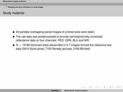
Mixed-effects models prediction
Modelling tree-level reflectance on aerial images
Study material
20 partially overlapping aerial images of a forest area were taken.
The raw data was postprocessed to provide (atmospherically corrected)reflectance data on four channels: RED, GRN, BLU and NIR.
N = 15188 dominant trees discernible in 2-7 images formed the reference treedata (5914 Scots pines, 7105 Norway spruces, 2169 Birches)
Individual trees on different images were using automatically matched.
The individual pixels within tree crowns were divided to sunlit and self-shadedpixels. The mean reflectances in these parts were analyzed separately -> asystem of 8 models (4 channels, shaded and sunlit) for each of the three treespecies.
Mehtätalo Mixed-effects models prediction

Mixed-effects models prediction
Modelling tree-level reflectance on aerial images
Structure of aerial image data on a forest
Observations from a given image are similar due to e.g. the properties of theatmosphere at the time of imaging and the atmospheric correction.
Repeated measurements of a certain tree are correlated due to tree-specificproperties.The model for each response and tree species has the following structure
yit = f (x it |b) + αi + αt + εit ,
where i and t refer to image and tree effects, respectively. σ2i and σ2
t are thecorresponding variances. The predictors are trigonometric transformations of thehorizontal and vertical viewing and Sun angles.The random effects at different levels of grouping are independent, therefore
var(yit ) = σ2i + σ2
t + σ2
cov(yit , yi′ t′) = 0
cov(yit , yit′) = σ2i
cov(yit , yi′ t ) = σ2t
Mehtätalo Mixed-effects models prediction

Mixed-effects models prediction
Modelling tree-level reflectance on aerial images
Structure of aerial image data on a forest
Observations from a given image are similar due to e.g. the properties of theatmosphere at the time of imaging and the atmospheric correction.Repeated measurements of a certain tree are correlated due to tree-specificproperties.
The model for each response and tree species has the following structure
yit = f (x it |b) + αi + αt + εit ,
where i and t refer to image and tree effects, respectively. σ2i and σ2
t are thecorresponding variances. The predictors are trigonometric transformations of thehorizontal and vertical viewing and Sun angles.The random effects at different levels of grouping are independent, therefore
var(yit ) = σ2i + σ2
t + σ2
cov(yit , yi′ t′) = 0
cov(yit , yit′) = σ2i
cov(yit , yi′ t ) = σ2t
Mehtätalo Mixed-effects models prediction

Mixed-effects models prediction
Modelling tree-level reflectance on aerial images
Structure of aerial image data on a forest
Observations from a given image are similar due to e.g. the properties of theatmosphere at the time of imaging and the atmospheric correction.Repeated measurements of a certain tree are correlated due to tree-specificproperties.The model for each response and tree species has the following structure
yit = f (x it |b) + αi + αt + εit ,
where i and t refer to image and tree effects, respectively. σ2i and σ2
t are thecorresponding variances. The predictors are trigonometric transformations of thehorizontal and vertical viewing and Sun angles.
The random effects at different levels of grouping are independent, therefore
var(yit ) = σ2i + σ2
t + σ2
cov(yit , yi′ t′) = 0
cov(yit , yit′) = σ2i
cov(yit , yi′ t ) = σ2t
Mehtätalo Mixed-effects models prediction

Mixed-effects models prediction
Modelling tree-level reflectance on aerial images
Structure of aerial image data on a forest
Observations from a given image are similar due to e.g. the properties of theatmosphere at the time of imaging and the atmospheric correction.Repeated measurements of a certain tree are correlated due to tree-specificproperties.The model for each response and tree species has the following structure
yit = f (x it |b) + αi + αt + εit ,
where i and t refer to image and tree effects, respectively. σ2i and σ2
t are thecorresponding variances. The predictors are trigonometric transformations of thehorizontal and vertical viewing and Sun angles.The random effects at different levels of grouping are independent, therefore
var(yit ) = σ2i + σ2
t + σ2
cov(yit , yi′ t′) = 0
cov(yit , yit′) = σ2i
cov(yit , yi′ t ) = σ2t
Mehtätalo Mixed-effects models prediction

Mixed-effects models prediction
Modelling tree-level reflectance on aerial images
The multivariate model
The multivariate model for a tree species is
y1it = f1(x it |b1) + α1i + α1t + ε1it
y2it = f2(x it |b2) + α2i + α2t + ε2it
...
y8it = f8(x it |b8) + α8i + α8t + ε8it
or simplyy it = f (x it |b) + αi + αt + εit
where the responses 1-8 refer to the sunlit and self-shaded pixels of the four channelsand
(α1i , α2i , . . . , α8i )′ = αi ∼ MVN(0,A8×8) include the random image-effects
(α1t , α2t , . . . , α8t )′ = αt ∼ MVN(0,B8×8) include the random tree-effects
(ε1it , ε2it , . . . , ε8it )′ = εit ∼ MVN(0,E8×8) include the random vector residuals
Now
var(y it ) = A + B + E
cov(y it , y i′ t′) = 0
cov(y it , y it′) = A
cov(y it , y i′ t ) = B
Model fitting (based on REML) yields b, A, B and E
Mehtätalo Mixed-effects models prediction

Mixed-effects models prediction
Modelling tree-level reflectance on aerial images
Estimated variance components (covariances not shown)
sunlit shade sunlit shade sunlit shade sunlit shade
Fixed (Xβ)-% 33 11 32 13 45 29 7 -0
Tree-% 42 42 43 41 18 13 62 64
Image-% 4 12 5 14 27 46 6 2
Residual-% 21 35 20 32 10 13 25 34
Total 100 100 100 100 100 100 100 100
Variance components, real data, 200 000 observations (%)
* Fixed part: The anisotropy trends explained SL >> SS, BLU > GRN > RED > NIR. In NIR, anisotropy is low. * Tree-effect: The correlations are strong, both for SL and SS. A bright tree is bright across views and bands. In NIR > 60% of variance explained!! * Image-effect: Substantial in BLU, SS > SL. Includes effects from solar elevation changes (07-09 GMT), atmospheric correction errors.
Ilkka Korpela, Oct 2012
Mehtätalo Mixed-effects models prediction

Mixed-effects models prediction
Modelling tree-level reflectance on aerial images
The use in classification
Let y it be an observed vector (length=8) of the reflectances of one tree t on the 8channels on one image i . The squared Mahalanobis distance between y it andµit is
d2it = (y it − µit )
′(A + B + E)−1(y it − µit )
This distance takes into account the correlation of reflectance among differentchannels, and is (at least under multivariate normality of the reflectance data) ina way optimal for single tree on single image.
For multiple images, the squared Mahalanobis distance between y ·t and µ·t is
d2·t = (y ·t − µ·t )
′D−1·t (y ·t − µ·t ) ,
where y ·t = (y ′1t , . . . , ymt ) is an observed vector (with length of 8m) of thereflectances of tree t on the 8 channels of m images. The 8m × 8mvariance-covariance matrix is
D·t =
A + B + E B . . . B
B A + B + E B...
. . ....
B B . . . A + B + E
This distance takes into account the correlation arising from the common treeeffectsExtension to many trees and images would be possible as well.
Mehtätalo Mixed-effects models prediction

Mixed-effects models prediction
Modelling tree-level reflectance on aerial images
The use in classification
Let y it be an observed vector (length=8) of the reflectances of one tree t on the 8channels on one image i . The squared Mahalanobis distance between y it andµit is
d2it = (y it − µit )
′(A + B + E)−1(y it − µit )
This distance takes into account the correlation of reflectance among differentchannels, and is (at least under multivariate normality of the reflectance data) ina way optimal for single tree on single image.For multiple images, the squared Mahalanobis distance between y ·t and µ·t is
d2·t = (y ·t − µ·t )
′D−1·t (y ·t − µ·t ) ,
where y ·t = (y ′1t , . . . , ymt ) is an observed vector (with length of 8m) of thereflectances of tree t on the 8 channels of m images. The 8m × 8mvariance-covariance matrix is
D·t =
A + B + E B . . . B
B A + B + E B...
. . ....
B B . . . A + B + E
This distance takes into account the correlation arising from the common treeeffects
Extension to many trees and images would be possible as well.
Mehtätalo Mixed-effects models prediction

Mixed-effects models prediction
Modelling tree-level reflectance on aerial images
The use in classification
Let y it be an observed vector (length=8) of the reflectances of one tree t on the 8channels on one image i . The squared Mahalanobis distance between y it andµit is
d2it = (y it − µit )
′(A + B + E)−1(y it − µit )
This distance takes into account the correlation of reflectance among differentchannels, and is (at least under multivariate normality of the reflectance data) ina way optimal for single tree on single image.For multiple images, the squared Mahalanobis distance between y ·t and µ·t is
d2·t = (y ·t − µ·t )
′D−1·t (y ·t − µ·t ) ,
where y ·t = (y ′1t , . . . , ymt ) is an observed vector (with length of 8m) of thereflectances of tree t on the 8 channels of m images. The 8m × 8mvariance-covariance matrix is
D·t =
A + B + E B . . . B
B A + B + E B...
. . ....
B B . . . A + B + E
This distance takes into account the correlation arising from the common treeeffectsExtension to many trees and images would be possible as well.
Mehtätalo Mixed-effects models prediction

Mixed-effects models prediction
System of mixed-effects model for aerial forest inventory
Motivation
Airborne Laser Scanners (ALS) provide information on the 3D- structure of forest
Majority of large individual trees can be detected from an ALS point cloud
Point cloud characteristics can be assigned to field-measured treecharacteristics to estimate a system of predictive models for tree characteristics,such as stem volume, height, diameter, crown base height, dead crown height.
These tree-specific characteristics are correlated within a forest stand
Also the stand effects are correlated across models
These correlations can be utilized to predict the random effects of amixed-effects model for a given stand for all 5 models using even oneobservation of one characteristics only
Enables improved predictions of hard-to-measure characteristics by usingeasy-to-measure characteristics
Mehtätalo Mixed-effects models prediction

Mixed-effects models prediction
System of mixed-effects model for aerial forest inventory
The model
The model includes a system of 5 mixed-effects models of form for tree i in stand k :
y1ki = a1 + b1x1ki + . . .+ α1k + β1k x1ki + ε1ki
y2ki = a2 + b1x2ki + . . .+ α2k + β2k x2ki + ε2ki
...
y5ki = a5 + b5x5ki + . . .+ α5k + β5k x5ki + ε5ki
where the fixed parts are as with the previous mixed-effects models and include theALS-based predictors.
The assumptions on the random effects and residuals are(α1k , β1k , α2k , β2k , . . . , α5k , β5k )′ ∼ MVN(0,D10x10), and(ε1k1, ε2ki , . . . , ε5ki ) ∼ MVN(0,R5x5)
The intended use of the model is prediction applying the random effects.
The previously presented principles were used to predict the random effects ofthe model system by using 1-10 sample trees per stand and 3 differentmeasurement strategies
Mehtätalo Mixed-effects models prediction

Mixed-effects models prediction
System of mixed-effects model for aerial forest inventory
Results2.
702.
802.
90
RMSE
DB
H,c
m
● ● ● ● ● ● ●●●
●
●
●
●●
● ●
● ●
Fixed part onlyDBHDBH+HCB+HDBDBH+HCB+HDB+H
0.75
0.77
0.79
H,m
● ● ● ● ● ● ●● ● ● ●● ● ●
0.12
00.
130
V,m
3
● ● ● ● ● ● ●
●
●
● ●
● ● ●
1.4
1.6
1.8
2.0
2.2
HD
B,m
● ● ● ● ● ● ●
●● ● ● ● ● ●
1.34
1.38
1.42
HC
B,m
● ● ● ● ●●
●
● ● ● ●● ●
●
1.8
2.0
2.2
2.4
Sample size
HC
B−
HD
B,m
2 4 6 8 10
● ● ● ● ● ● ●
●● ● ● ● ● ●
0.0
0.2
0.4
0.6
bias
● ● ● ● ● ● ●
●
●
●●
●● ●
−0.
03−
0.01
0.01
Sample size
● ● ● ●●
● ●
●
●
●●
●● ●
0.00
0.02
0.04
Sample size
● ● ● ● ● ● ●
●●
● ●● ● ●
−1.
2−
0.8
−0.
40.
0
Sample size
● ● ● ● ● ● ●● ● ● ● ● ● ●
−0.
010.
01
Sample size
t
● ● ●● ● ● ●
●●
●●
● ●●
0.0
0.4
0.8
1.2
Sample size
2 4 6 8 10
● ● ● ● ● ● ●● ● ● ● ● ● ●
Mehtätalo Mixed-effects models prediction