COMPARATIVE ANALYSIS OF ADVANCED · PDF fileof optimizing the mobile radio path loss model is...

http://www.iaeme.com/IJARET/index.asp 50 [email protected]

International Journal of Advanced Research in Engineering and Technology (IJARET) Volume 8, Issue 4, July - August 2017, pp. 50–74, Article ID: IJARET_08_04_006

Available online at http://www.iaeme.com/IJARET/issues.asp?JType=IJARET&VType=8&IType=4

ISSN Print: 0976-6480 and ISSN Online: 0976-6499

© IAEME Publication

COMPARATIVE ANALYSIS OF ADVANCED

STATISTICAL TECHNIQUES FOR

OPTIMIZATION OF HYBRID MOBILE RADIO

PATH LOSS MODEL

A. Bhuvaneshwari

Department of Electronics and Communication Engineering,

Deccan College of Engineering and Technology, Hyderabad, Telangana, India

R. Hemalatha

Department of Electronics and Communication Engineering

Osmania University, Hyderabad, Telangana, India

T. Satya Savithri

Department of Electronics and Communication Engineering

Jawaharlal Nehru Technological University, Hyderabad, Telangana, India

ABSTRACT

Path loss optimization is an important requirement in the design and

implementation phase of mobile radio systems. The accuracy of the propagation

model is improved by optimizing the model parameters to reflect the real time

environment in a better manner. The paper aims at optimizing the proposed hybrid

Walfisch–Ikegami path loss model for cellular signals in urban environment. The

hybrid model is optimised with traditional method of Multiple Linear Regression and

advanced statistical techniques of Ridge and Robust Regression. Although the

techniques are used for other applications, evaluating the performance in the context

of optimizing the mobile radio path loss model is a novel idea. The statistically

developed optimized path loss models are validated by field strength measurements.

The performances of the optimised models are evaluated in terms of path loss, error

metrics and Goodness of Fit (GOF) tests. The Ridge optimized path loss model gives

the least values of Prediction error (1.1701), RMSE (0.0827) and other error metrics.

The Goodness of Fit tests additionally validates the efficient performance of Ridge

optimized path loss model.

Key words: Hybrid Walfisch-Ikegami model, Multiple Linear Regression, Ridge

Regression, Robust Regression, Prediction error, Relative error

Cite this Article: A. Bhuvaneshwari, R. Hemalatha, T. Satya Savithri. Comparative

Analysis of Advanced Statistical Techniques for Optimization of Hybrid Mobile

Radio Path Loss Model. International Journal of Advanced Research in Engineering

and Technology, 8(4), 2017, pp 50–74.

http://www.iaeme.com/IJARET/issues.asp?JType=IJARET&VType=8&IType=4

A. Bhuvaneshwari, R. Hemalatha, T. Satya Savithri


1. INTRODUCTION

The recent advancement in cellular technology has increased the number of mobile phone

users to a large extent. It is required to ensure a better quality of service to the subscribers

with efficient planning and design of mobile radio network. Site specific path loss modeling is

an important aspect of cellular design which involves the signal measurements in a particular

terrain in order to estimate the average signal loss along the propagation path. The

propagation path loss models are mathematical tools that quantify the mean signal strengths at

a given distance from the transmitter in a particular location [1]. The parameters of the

propagation model are tuned or optimized to reflect the exact characteristics of the medium

through which the signals propagate. The model tuning or optimization process aims at

minimizing the differences between the predicted and measured field strengths [2]. The

objective of tuning the propagation model is achieved when the estimations made by the

optimized model has a better agreement with the real time measurements compared to the un

tuned model.

In the earlier work, several tuning approaches are implemented on empirical and semi-

empirical path loss models and their performances are evaluated. The Okumura Hata model is

modified and tuned based on Levenberg-Marquardet algorithm by Akhoondzadeh-Asl, L. and

Noori [3]. An optimized Cost-231 Hata model for suburban and urban environments was

developed by Mardeni and Sivapriya [4]. A linear-iterative method using least square theory

was used to tune Cost-231 Hata model by Chhaya Dalela, Prasad and P. K. Dalela [5]. The

empirical models are not very accurate since they do not consider wave guiding effects and

require large measurement data. On the other hand, the semi deterministic propagation models

combine deterministic aspects along with empirical measurements. The least square method

was used by Mousa etal to tune a macrocell model and semi deterministic Walfisch-Bertoni

model [6]. Tahat and Taha used particle swarm optimization for tuning Walfisch-Ikegami

(WI) model [7]. Statistical tuning of Walfisch Ikegami model was performed by Slawomir J.

Ambroziak and Ryszard J. Katulski [8]. Ambawade, Dayanand, et al have optimized the

parameters of Walfisch-Ikegami model using statistical Multiple Linear Regression [9]. Most

of the discussed optimization techniques are implemented on the existing empirical or semi

empirical propagation models.

In this paper a proposed semi deterministic hybrid Walfisch Ikegami (WI) model is

considered for optimization. The proposed hybrid model combines the statistical variations of

the original Walfisch Ikegami model and the deterministic approach of ray tracing method for

the purpose of modeling multiple reflection losses [10]. The hybrid model has a better

performance in estimating the path loss of the mobile radio signals and the results are

validated by field measurements [10]. Although the hybrid model exhibits a better

performance, there exists a scope of optimizing the model parameters to have more accurate

prediction results.

The highlight of the work is to optimize the proposed semi deterministic hybrid Walfisch

Ikegami path loss model with advanced statistical methods of Ridge and Robust Regressions.

The performance of the optimized models is compared with the traditional tuning of Multiple

Linear Regression. The major drawback of Multiple Linear Regression method is it does not

consider the deviations in the assumptions and compromises on the stability of the estimates.

Secondly the presence of outliers in the data to be analyzed significantly affects the least-

squares linear fitting [11]. Hence advanced statistical methods such as Ridge and Robust

regressions are used to optimize the model parameters. The Ridge Regression improves the

prediction results, in the presence of unstable estimates when a large collinearity exists

Comparative Analysis of Advanced Statistical Techniques for Optimization of Hybrid Mobile

Radio Path Loss Model


between the independent variables [11]. To minimize the influence of data outliers, Robust

Regression is used to optimize the hybrid Walfisch Ikegami model.

Although the Ridge and Robust regression methods are used in various applications,

employing them in the context of optimizing the proposed semi deterministic hybrid mobile

radio path loss model is a novel idea. The optimized models are validated by GSM signal

measurements collected at 900 MHz in the dense urban region of Hyderabad city in

Telangana state. A comparative analysis of the optimized models is made and Ridge

optimized model is found to estimate the path loss in a more precise manner for the specified

scenario. The paper is organized as follows. Section 1 gives the Introduction. Section 2

describes the proposed semi deterministic hybrid Walfisch Ikegami model and the

methodology of optimizing the model. Section 3 explains the optimization procedure with

commonly used Multiple Linear Regression and advanced methods of Ridge Regression and

Robust Regression. Section 4 briefly describes the performance evaluation metrics. Section 5

includes the simulation results, statistical analysis of each method, validation of the optimized

models and comparison. Section 6 has the conclusions and future scope.

2. SEMI DETERMINISTIC HYBRID WALFISCH IKEGAMI MODEL

AND ITS OPTIMISATION

A semi deterministic hybrid Walfisch Ikegami model is developed by merging the statistical

variations of the original WI model and deterministic method of ray tracing. The parameters

in the original WI model which are statistically altered are height of the buildings (hroof),

separation between the buildings (s), and the street orientation angle ( . These parameters

are modelled as Gaussian random variables with specified limits since they are not uniform

and may vary in the dense urban region. The parameters are influenced by the terrain clutter

and are modelled by Gaussian distribution with a mean and standard deviation (σ) to obtain

better prediction. The modified parameters are given as [10]

( (

( (1)

are the normalised random variables, are

the respective means and and are the corresponding standard deviations.

Knowing the modified parameters, the new values of multi screen diffraction loss ( ),

function of street orientation angle( ) and roof top to street diffraction loss ( used in

the path loss calculation of Walfisch Ikegami model are estimated as [7][10]

( ( – ( (2)

( (3)

( ( (4)

The altered terms are substituted in the original Cost 231 Walfisch-Ikegami model and the

statistically modified Walfisch Ikegami path loss equation is given as [10]

(5)

is free space loss, „w‟ is the street width, , „ is the modified separation parameter

between the buildings, is statistically modified building height, is the diffraction

loss factor, is the distance factor, is the frequency factor, „f‟ is the frequency of



operation and „d‟ is the distance factor. Although the modified loss parameters ensure better

path loss prediction, the above equation retains the major drawback of neglecting the multiple

reflection losses from the buildings along the propagation path. In order to overcome this

drawback, a deterministic image method of ray tracing is used to obtain the power received

due to multiple reflections by implementing an N ray tracing model. A detailed image method

of ray tracing is presented in paper [10]. The received power due to multiple reflections

( is estimated using image method of ray tracing by selecting „n‟ valid rays within a

specified threshold and is given as [10].

(

) ∑

(6)

Where ( is the phase difference in terms of path length xi, wavelength

( ), Ri is the reflection coefficient for each path, at and ar are the directional functions of

transmitter, receiver and is the transmitted power. Knowing the transmitted and received

power, the path loss due to multiple reflections is given as

(

) (7)

The path loss due to multiple reflections is included in the statistically modified Walfisch

Ikegami model given in Equation 5 and the expression for the proposed hybrid Walfisch

Ikegami path loss model is given as

( (8)

The path loss estimated by the hybrid model has a better performance compared to the

original model as validated by error metrics [10]. In order to further improve the path loss

prediction, the parameters of the proposed hybrid model is optimised using Multiple Linear

Regression and advanced statistical methods of Ridge and Robust Regressions.

2.1. Optimisation of Semi Deterministic Hybrid Walfisch Ikegami Model

In wireless mobile communications, the optimisation of the propagation model is very useful

for overcoming several constraints and to ensure end to end quality of service to the users.

Model tuning or optimization is a process in which, the model parameters are adjusted or

optimized as per the desired environment in order to have a best agreement between the

predictions and measurements. Tuning a propagation model makes it more accurate for

predicting the received signal strengths [12]. The optimisation of the propagation model

ensures that handoff points closely match with the prediction, the coverage is within the

specified guidelines and the co-channel interference is low at adjacent sites [13].

The major contribution in the paper is optimising the parameters of the proposed hybrid

WI model. The general tuning methodology is described as follows. The proposed hybrid

Walfisch Ikegami model as per Equation 8 is given as

( (9)

Substituting the terms in the above path loss Equation, it is re written as [10]

(

( ( – (

(10)

Knowing the transmitted power ( , equation for received power ( is given as




(

(

( ( ( (11)

is the power lost by multiple reflections computed from the image method of ray

tracing [10]. The free space loss is given as

( ( (12)

Substituting the free space loss, the Equation 11 is re written as

( (

( (

(

( ( (13)

is the received power of the hybrid model, and rearranging the terms in the above

equation gives

( ( (

( ( ( ) (The term with distance parameter)

( ( (The term with the building separation parameter„s‟)

( ( ( (The term representing heights)

( (The term representing the street orientation)

(The power lost by multiple reflections computed by ray tracing) (14)

The above equation is written as

(15)

is the optimised received power and as per Equation 14 it describes the four

terms to be optimised with parameters of distance (d), separation between the buildings (s),

roof height ( , and street orientation angle ( . The corresponding coefficient estimates

( are obtained by traditional method of Multiple Linear Regressions and

comparison is made with estimates obtained by Ridge and Robust regression methods.

Knowing the optimised received power (

and transmitted power ( ) the

optimised hybrid path loss model is given as

(

) (

) (16)

Equation 16 is the optimised hybrid path loss model. Depending on the method of

obtaining the coefficient estimates, three optimised models are developed to estimate the path

loss.



3. STATISTICAL OPTIMISATION TECHNIQUES

The optimization problem is defined by an objective function and a set of constraints on the

variables of the function. It is required to obtain the optimum values of the variables by either

minimizing or maximizing the function, and simultaneously satisfying all the constraints.

Several iterations are done until an optimum result is obtained. This paper analyses the

performances of commonly used MLR technique with advanced statistical methods of Ridge

and Robust Regressions in the context of optimising the path loss. The flow charts and

functional operations of the techniques are discussed in this section.

3.1. Optimisation using Multiple-Linear Regression

Least square regression technique is a simplest and most commonly used prediction method

which provides a linear line fit for a specified set of observations. But it does not provide the

best results when the parameters in the training data have random variations. The least square

method also results in poor predictions when the independent variables are more correlated to

each other [11]. The multiple linear regressions are an extended version of a simple linear

regression model, in which the prediction equation has various independent variables related

to the dependent variable. The multi linear regression equation in general form is given as

[14]

(17)

are the regression coefficients to be estimated for a set of variables. The

regression coefficients are obtained as least square estimates which minimises the residual

sum of squares [14]. The regression model is of the form [15]

(18)

In matrix notation it is given as [14]

[ ]

[

]

[ ]

[ ]

(19)

Y is a n×1 dimensional random vector representing the observations, X is an n×(k×1)

matrix determined by the predictors, is a (k+1)×1 vector of unknown regression coefficients

and e indicates the random errors. The optimisation of a path loss model using Multiple

Linear Regressions requires obtaining solution to the equation given as [14]

(20)

[ ] (21)

[ ] (22)

X is a matrix of independent variables that has to be optimised. Y is a matrix of

measurement data as dependent variables. is a vector of least square estimators or the tuning

coefficients for optimising the model. This optimisation method creates the relationship as per

Equation 18, as a linear line that provides a best approximation of all the data points. The

flowchart for Multiple Linear Regression is shown in Figure 1.




Figure 1 Multiple Linear Regressions

The steps in Multiple Linear Regressions are summarised

The first step is to obtain a matrix (X) of independent variables and a matrix (Y) of a

dependent variable, comprising of the measurement data.

Compute the product of the matrix X with its transpose( .

Apply inverse to the obtained result.

Compute the product of the matrix Y with the transpose of the matrix X.

Multiply the results obtained from steps 3 and 4. The values of gives the regression

coefficients.

Implementing Multiple Linear Regressions for the Hybrid Walfisch Ikegami model, the

equation of the received power in terms of the dependent and independent parameters is

written from Equation 14 as

( ( ( ( (23)

is the received power of MLR optimised hybrid model,

A is a constant term given as

( ( (24)

( ( (

( (

( ( (

(

are the coefficient estimates obtained from Multiple Linear regression. The

optimised received power is converted into path loss as per Equation 16 and the MLR

optimised hybrid path loss model is given as

(

) (

) (25)

Although this technique is a flexible method that provides optimum results, the coefficient

estimates fluctuates due to multi collinearity and the presence of outliers in the data. Hence

advanced statistical methods of Ridge and Robust Regressions are employed for better

optimisation.



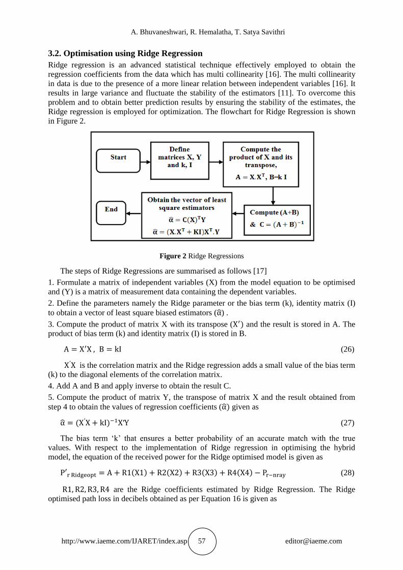
3.2. Optimisation using Ridge Regression

Ridge regression is an advanced statistical technique effectively employed to obtain the

regression coefficients from the data which has multi collinearity [16]. The multi collinearity

in data is due to the presence of a more linear relation between independent variables [16]. It

results in large variance and fluctuate the stability of the estimators [11]. To overcome this

problem and to obtain better prediction results by ensuring the stability of the estimates, the

Ridge regression is employed for optimization. The flowchart for Ridge Regression is shown

in Figure 2.

Figure 2 Ridge Regressions

The steps of Ridge Regressions are summarised as follows [17]

1. Formulate a matrix of independent variables (X) from the model equation to be optimised

and (Y) is a matrix of measurement data containing the dependent variables.

2. Define the parameters namely the Ridge parameter or the bias term (k), identity matrix (I)

to obtain a vector of least square biased estimators ( ) .

3. Compute the product of matrix X with its transpose ( and the result is stored in A. The

product of bias term (k) and identity matrix (I) is stored in B.

(26)

is the correlation matrix and the Ridge regression adds a small value of the bias term

(k) to the diagonal elements of the correlation matrix.

4. Add A and B and apply inverse to obtain the result C.

5. Compute the product of matrix Y, the transpose of matrix X and the result obtained from

step 4 to obtain the values of regression coefficients ( given as

( (27)

The bias term „k‟ that ensures a better probability of an accurate match with the true

values. With respect to the implementation of Ridge regression in optimising the hybrid

model, the equation of the received power for the Ridge optimised model is given as

( ( ( ( (28)

are the Ridge coefficients estimated by Ridge Regression. The Ridge

optimised path loss in decibels obtained as per Equation 16 is given as




(

) (

) (29)

The accuracy of the Ridge estimates largely depends on choosing an accurate value of

Ridge parameter (k) which is generally obtained from the Ridge trace [17]. The Ridge

estimators are biased and more stable than the unbiased least square estimators [18] . This

produces reliable results in the presence of multi collinearity.

3.3. Optimisation using Robust Regression

The experimental data sets used in the analysis, generally consists of missing data, outliers,

unstable variances and deviations from assumptions which result in poor prediction. The

extreme data points or left over data points called outliers have a significant effect on the fit,

because their effects are magnified on squaring the residual errors [19]. Robust Regression is

the best solution to minimize the effect of outliers and is much better than least square

estimation, when the data to be analysed has outliers [19]. This regression method is

insensitive to small deviations in assumptions. A linear model with „n‟ observations, with as the dependent variable, as independent variables is given as [20]

(30)

is the intercept, are the regression coefficients, is the error term that

gives the difference between the predicted values and the dependent variable . The fitted

model of Equation 30 is given as

( (

) (31)

is the objective function to be minimised. A group of estimators called M estimators

was developed by Huber, given as [20].

∑ (

(32)

is a symmetric function with a minimum at zero. The general M-estimator that

minimizes the objective function is given as [21]

∑ ( ∑ (

) (33)

The objective function is differentiated with respect to the coefficients „ ‟ and the partial derivatives set to zero. The derivative of is given as and the resulting k+1

estimating equations for the coefficients are given as

∑ (

(34)

The estimating equations are rewritten by defining a weight function ( (

∑ (

(35)

The estimating equations are solved by Iterative Reweighted Least Squares (IRLS)

method to obtain M Robust estimates [21].

The feasibility of using Robust Regression for improving the path loss prediction is

checked and the expression for Robust optimised received power is given as

( ( ( ( (36)



are the coefficient estimates obtained by Robust Regression.

Knowing the optimised received power the path loss as per Equation 16 is given as

(

) (

) (37)

is the path loss in decibels of the hybrid model optimised by using

Robust regression.

4. PERFORMANCE EVALUATION OF THE OPTIMISATION

TECHNIQUES

The performance of the optimized models is evaluated by comparing the model estimated

path loss with the loss obtained from measurements. Comparisons are made in terms of error

statistics such as Prediction Error ( , Mean Square Error (MSE), Root Mean Square Error

(RMSE), Spread Corrected RMSE (SC-RMSE), and percentage relative error. The

performance of the optimization techniques are also evaluated in terms of Goodness of Fit

(GOF) Tests. The error metrics and statistics of GOF tests are summarized in Table1.

Table 1 Performance Evaluation metrics

The measured path loss is taken as a reference to compute the error metrics. The

prediction error is the difference between the measured path loss and model predicted path

loss. The Root Mean Square Error (RMSE) is an important metric and a value closer to zero

Parameters Formulae

Prediction Error ( ) , is the measured Path Loss, is the model predicted Path Loss, N is the number

of observations

Mean Square Error (MSE)

∑ | |

Root Mean Square Error

(RMSE) √

Standard Deviation (SD)

( σ √

∑ (

ME is the

mean error

Spread Corrected RMSE

(SC-RMSE)

√

∑

Relative Error (%)

Statistics of Goodness of Fit

Sum of Squares Due to

Error (SSE) ∑

| |

R-square

SST is sum squares about

the mean

Adjusted R-square

(

( , v = n-m

v is the residual degrees of freedom, „n‟ are the

number of response values and „m‟ is the number

of fitted coefficients.




indicates a better fit [22]. The Standard Deviation (SD) is a measure of variability or

dispersion. A low standard deviation indicates that the data points are very close to the mean,

and a high standard deviation indicates the spreading of data over a large range of values. The

spread corrected RMSE is a measure of dispersion of overall error [22].

The variation of the model parameters before and after optimisation is evaluated in terms

of Goodness of Fit (GOF) Tests. The GOF statistics are Sum of Squares due to error (SSE),

R-square and Adjusted R-square [23]. The SSE statistical measure indicates the total

deviation of the predicted values from the fit. A value of SSE closer to zero suggests that the

model has a small random error value and the fit is more useful for prediction [23]. The R-

Square statistic explains how good the fit is with respect to the variation of data. R- Square

values lies between 0 and 1and a value close to 1 indicates that there is more variation in the

data with respect to the average. The adjusted R Square is a best measure of the quality of the

fit and a value closer to 1 indicates a better fit [23].

5. RESULTS AND DISCUSSIONS

The propagation models must estimate the path loss with a maximum accuracy to reflect the

actual environment where the propagation takes place. Drive tests are conducted in the region

of interest to find out the correction factors to be included in the model. The model parameters

are tuned using various optimization techniques to obtain better prediction results. The

performances of the optimized models are evaluated by comparison with real time

measurements. In this paper, a drive test is done in the dense urban region of Hyderabad city

of Telangana state in Southern India. The received mobile signal strengths are collected at a

downlink frequency of 947.5 MHz using Test Mobile System (TEMS) tool by traversing

across ten locations of base stations from Ameerpet to Secunderabad in Hyderabad city

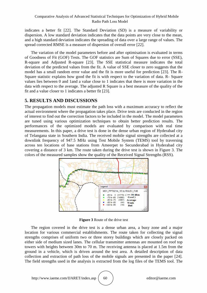
covering a distance of 3 km. The route taken during the drive test is shown in Figure 3. The

colors of the measured samples show the quality of the Received Signal Strengths (RSS).

Figure 3 Route of the drive test

The region covered in the drive test is a dense urban area, a busy zone and a major

location for various commercial establishments. The route taken for collecting the signal

strengths comprises of uniform two or three storey buildings which are closely packed on

either side of medium sized lanes. The cellular transmitter antennas are mounted on roof top

towers with heights between 30m to 70 m. The receiving antenna is placed at 1.5m from the

ground in a vehicle, which is driven around the test area. A detailed description of data

collection and extraction of path loss of the mobile signals are presented in the paper [24].

The field strengths used in the analysis is extracted from the log files of the TEMS tool. The



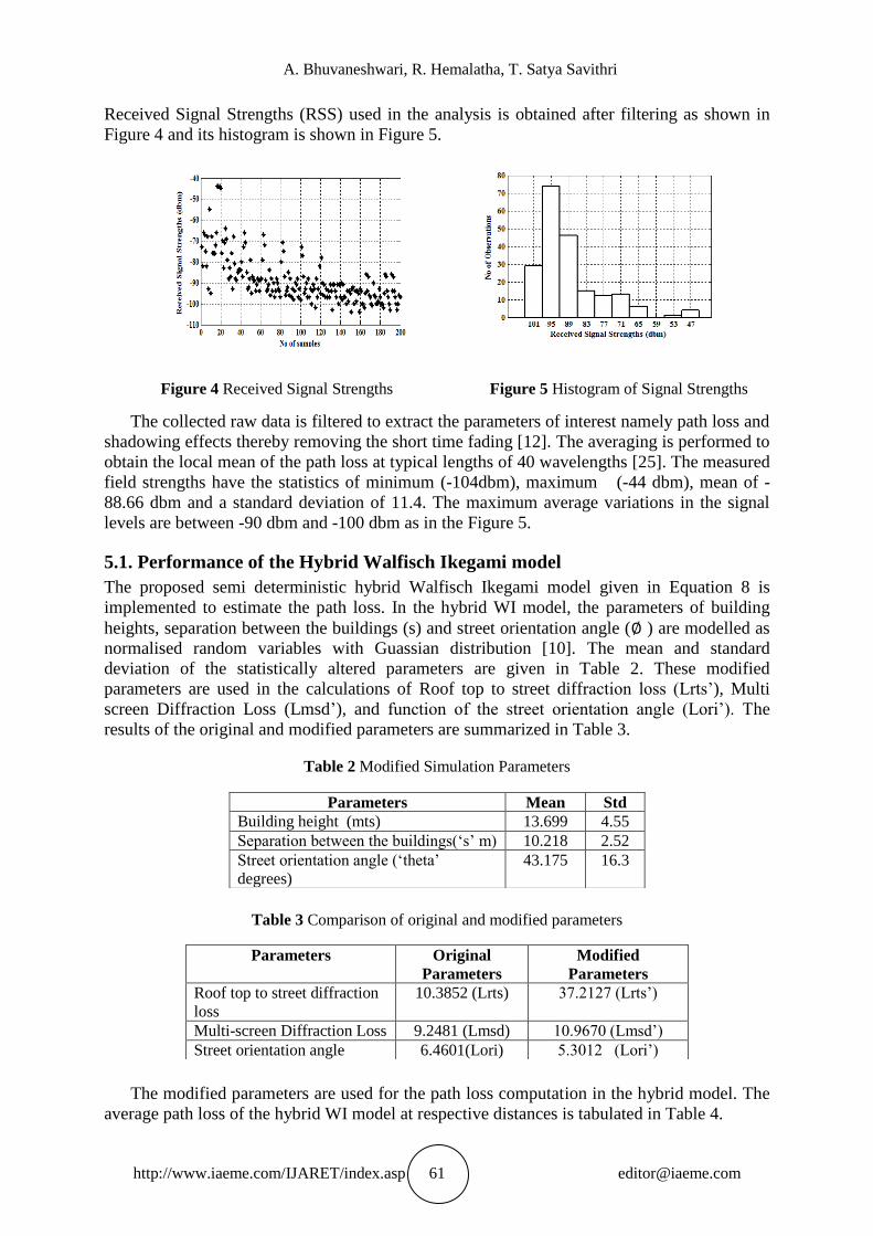
Received Signal Strengths (RSS) used in the analysis is obtained after filtering as shown in

Figure 4 and its histogram is shown in Figure 5.

Figure 4 Received Signal Strengths Figure 5 Histogram of Signal Strengths

The collected raw data is filtered to extract the parameters of interest namely path loss and

shadowing effects thereby removing the short time fading [12]. The averaging is performed to

obtain the local mean of the path loss at typical lengths of 40 wavelengths [25]. The measured

field strengths have the statistics of minimum (-104dbm), maximum (-44 dbm), mean of -

88.66 dbm and a standard deviation of 11.4. The maximum average variations in the signal

levels are between -90 dbm and -100 dbm as in the Figure 5.

5.1. Performance of the Hybrid Walfisch Ikegami model

The proposed semi deterministic hybrid Walfisch Ikegami model given in Equation 8 is

implemented to estimate the path loss. In the hybrid WI model, the parameters of building

heights, separation between the buildings (s) and street orientation angle ( ) are modelled as

normalised random variables with Guassian distribution [10]. The mean and standard

deviation of the statistically altered parameters are given in Table 2. These modified

parameters are used in the calculations of Roof top to street diffraction loss (Lrts‟), Multi

screen Diffraction Loss (Lmsd‟), and function of the street orientation angle (Lori‟). The

results of the original and modified parameters are summarized in Table 3.

Table 2 Modified Simulation Parameters

Table 3 Comparison of original and modified parameters

The modified parameters are used for the path loss computation in the hybrid model. The

average path loss of the hybrid WI model at respective distances is tabulated in Table 4.

Parameters Mean Std

Building height (mts) 13.699 4.55

Separation between the buildings(„s‟ m) 10.218 2.52

Street orientation angle („theta‟

degrees)

43.175 16.3

Parameters Original

Parameters

Modified

Parameters

Roof top to street diffraction

loss

10.3852 (Lrts) 37.2127 (Lrts‟)

Multi-screen Diffraction Loss 9.2481 (Lmsd) 10.9670 (Lmsd‟)

Street orientation angle 6.4601(Lori) 5.3012 (Lori‟)




Table 4 Path Loss of Hybrid Walfisch Ikegami model

The path loss predicted by the hybrid WI model has a mean value of 121.8db as compared

to 125.7 db of the path loss extracted from measurements. It has an improved performance

compared to the original Walfisch Ikegami model and a better match with the measured path

loss [10]. The error metrics computed for the hybrid WI model are found to have values of

Prediction error (3.0945), MSE (0.0479), RMSE (0.2188), Spread corrected-RMSE (0.6433),

Standard deviation of error (0.2177) and percentage relative error (3.19) [10]. The results

suggest an improvement in the performance of the hybrid model with respect to the original

Walfisch Ikegami model [10]. This improvement is due to the statistical modifications in the

original model and the inclusion of multiple reflection losses by ray tracing method. Although

the hybrid model has a better prediction, it can be further improved by optimizing the model

parameters.

5.2. Optimisation of Hybrid WI model by Multiple Linear Regressions

The parameters of the hybrid WI model are optimised using Multiple Linear Regressions. The

equation of the received power is rearranged in terms of four parameters X1, X2, X3, X4

which are to be optimised. The respective optimised coefficients are O1, O2, O3 and O4

which are computed from MLR technique. The term X1 is associated with distance, X2

specifies the separation between the buildings, X3 involves the height of the roof and the

receiving antenna height, which is used for Lrts calculations and X4 term is associated with

the orientation angle. The tuned coefficients obtained by MLR technique are multiplied with

the respective parameters to obtain the modified new values of X1new= X1*O1; X2new=

X2*O2; X3 new= X3*O3; X4new= X4*O4. The coefficients obtained from MLR are given in

Table 5. The absolute values of the parameters before and after tuning are summarised in

Table 6. Table 5 MLR Coefficients

Table 6 Statistics of Parameters before and after tuning

Distance

(kms)

Model predicted PL(db)

Hybrid W-I model

0.526 97.7010

1.012 114.9644

1.599 124.8332

2.077 130.7233

2.527 128.9605

2.880 133.7102

MLR

Coefficients O1 O2 O3 O4 A

0.6296 0.8194 -0.3733 0.6799 -84.0205

Statistics

X1 X2 X3 X4

X1 X1new X2 X2new X3 X3new X4 X4new

Min 0.196 0.124 4.966 4.069 0.021 0.007 0.171 0.116

Max 47.28 29.77 10.94 8.965 42.06 15.7 11.84 8.048

Mean 9.297 5.853 9.063 7.426 4.965 1.853 5.311 3.611

Std 8.079 5.086 0.968 0.793 5.888 2.198 1.975 1.343



From the results of Table 6, it is observed that after optimisation, the mean values of the

parameters are scaled and the variance is reduced.

5.2.1. MLR optimised Path Loss

The Multiple Linear Regression coefficients obtained in Table 5 are substituted in the

Equation 23 to obtain MLR optimised received power. From the optimised received signal

strengths the MLR optimised path loss is computed. A comparison graph showing the un

tuned path loss of the Hybrid WI model, MLR optimised path loss and experimentally

determined path loss are shown in Figure 6. The path loss values are tabulated in Table 7.

The mean value of the MLR optimized path loss is 122.6 which is a closer value to the

measured path loss. The mean path loss of the un tuned hybrid WI model differs by 3.9 db

from the measured value, whereas the MLR optimised path loss differs by 3.1 db.

Figure 6 MLR Optimised Path Loss

Table 7 Path Loss comparison

The optimization provides an improvement of 0.8 db in estimating the path loss. The

MLR optimized power has a standard deviation of 9.93 db as compared to 12.63 db of the

hybrid WI model before optimisation. This suggests that the tuning procedure decreases the

standard deviation. The optimization by Multiple Linear Regression provides reasonably good

results when the observation data is not too large.

5.3. Optimisation of Hybrid WI model by Ridge Regression

The hybrid WI model is optimized using advanced statistical method of Ridge Regression.

This method provides best results if the predictor variables are more linearly related,

indicating the presence of multi collinearity. Initially the extent of linear dependency between

the variables is assessed by correlation matrix, Variance Inflation Factor and Belsley

Collinearity Diagnostics [18][28]. Secondly the ridge trace is plotted to obtain the optimum

values of the Ridge coefficients. The estimated coefficients from the Ridge trace are used to

optimize the Hybrid WI model.

Path Loss

Models

Path Loss (db)

Min Max Mean

Measured PL 81 141 125.7

Hybrid W-I (un tuned) 70 138 121.8

MLR optimised 84 142 122.6




5.3.1. Multi Collinearity Detection

The regression coefficients largely depend on the contributions from the predictor variables. In order to assess

the linear relationships among the variables the multi collinearity diagnostics namely correlation matrix,

Eigen values and Variance Inflation Factors (VIF) are obtained [18]. The statistics are summarised in

Tables 8, 9 and 10.

Table 8 Correlation Matrix

Table 9 Eigen values

Table 10 Variance Inflation Factor

From the correlation matrix it is observed that, the correlation coefficients are very small

values, which suggest less dependency between the independent and dependent variables and

indicates that there is no strong multi collinearity. From the Eigen values, it can be said that at

least if one value differs by one and nearing to zero, there exists multi collinearity in the data

[26]. The Eigen values tabulated do not indicate strong multi collinearity. In Table 10, it is

observed that the values of Variance Inflation Factor are greater than one. Hence it can be

concluded that, there exists moderate multi collinearity in the data to be analyzed [27].

Additional statistics such as Belsley collinearity diagnostics which include singular values,

condition indices and variance decomposition proportion in a matrix form are presented in

Table 11.

Table 11 Belsley Collinearity Diagnostics

Correlation X1 X2 X3 X4

X1 1.000 0.1205 0.0383 0.0752

X2 0.1205 1.0000 0.1108 -0.0118

X3 0.0383 0.1108 1.000 -0.1227

X4 0.0752 -0.0118 -0.1227 1.0000

Eigen Values

=1 .1924

= 1.160

= 0.8553

=0.8363

VIF(X1) VIF(X2) VIF(X3) VIF(X4)

1.0021 1.0515 1.0290 1.0220

Singular

Values

Condition

Index

Var1 (X1) Var2 (X2) Var3(X3) Var4 (X4)

1.76 1 0.032 0.010 0.034 0.012

0.73 2.41 0.117 0.003 0.829 0.014

0.558 3.15 0.824 0.037 0.046 0.103

0.247 7.12 0.027 0.950 0.091 0.871

http://www.mathworks.com/help/econ/collintest.html#bucjrw5



Larger values of condition indices indicate more dependency and thereby do not produce

accurate regression. The variance decomposition proportion in the second row for X3 and last

row for X2 and X4 exceeds the default tolerance of 0.5 [28]. This suggests the presence of

multi collinearity in the parameters X2, X3 and X4 and justifies the use of Ridge Regression.

A plot of the correlations among the variables, their histograms and the scatter plots of the

variables are depicted in Figure 7.

Figure 7 Correlation plots of the variables

5.3.2. Selection of Ridge parameter (k) from the Ridge Trace

The Ridge regression coefficients are estimated by adding a small value of bias term „k‟ to the

diagonal elements of the correlation matrix. The Ridge regression shrinks the estimates

compared to Least Square Regression and the degree of shrinkage is controlled by the Ridge

parameter (k). The best suited value of the Ridge parameter (k) is obtained by a graphic

method called Ridge trace as suggested by Hoerl and Kennard [18]. The plot of Ridge trace is

shown in Figure 8.

Figure 8 Ridge Trace

The Ridge Trace is a graph of standardized regression coefficients ( on y axis and „k‟ values on x axis respectively. The value of „k‟ is chosen from the Ridge trace such that all the

ridge coefficients are stabilized at that value of „k‟ and the estimates do not change

significantly as k increases [29]. The optimum value of „k‟ is selected so that the residual sum

of squares is not too large compared to its minimum value [17]. In Figure 8, the Ridge




coefficients are selected at k=1100, represented by a dotted vertical line, where the Ridge

coefficients are stabilised. The bias increases as the shrinkage parameter (k) increases and

correspondingly the variance decreases. The estimated ridge coefficients at k=1100, for the variables X1,

X2, X3 and X4 are summarised in Table 12.

Table 12 Ridge Coefficients

5.3.3. Ridge Optimised Path Loss

The stabilised Ridge coefficients obtained from the Ridge trace is used to optimise the parameters in the

expression for received power as in Equation 28. The statistics of the parameters before and

after optimisation are summarised in Table 13.

Table 13 Statistics of Parameters before and after tuning

Comparing the parameters before and after tuning as in Table 13, it is found that the mean

values of the optimized parameters and their standard deviation is reduced after optimisation.

The Ridge optimized path loss is obtained according to Equation 29 and is plotted with

respect to the distance as shown in Figure 9. The mean values of the measured and model

predicted path loss in decibels are summarized in Table 14.

Figure 9 Ridge optimised Path Loss

Table 14 Path Loss comparison

Ridge

Coefficients

R1 R2 R3 R4 A

0.4798 0.3876 -0.0287 -0.6239 -84.115

Statistic

s

X1 X2 X3 X4


Min 0.196 0.094 4.966 1.925 0.021 5.961e-4 0.171 -0.072

Max 47.28 22.68 10.94 4.241 42.06 1.209 11.84 5.018

Mean 9.297 4.461 9.063 3.531 4.965 0.147 5.311 2.257

Std 8.079 3.876 0.968 0.3752 5.888 0.1692 1.975 0.839

Path Loss

Models

Path Loss (db)

Min Max Mean


Hybrid WI(un tuned) 70 138 121.8

Ridge optimised 103 136 127.4



The average value of the Ridge optimized path loss has a better agreement with the measured path loss. The

mean value of Ridge optimized path loss differs from the measured path loss by 1.7 db as

compared to 3.9 db for the original Hybrid WI model. The optimization provides a path loss

improvement of 2.2 db with respect to the predictions made with the un tuned model. This

improvement is due to the use of biased estimators in Ridge regression instead of unbiased

estimators as in MLR technique [18]. As a result of optimization, the standard deviation and

hence the variance of the tuned parameters are reduced, thereby increasing the precision of estimation and

the objective of Ridge regression is achieved.

5.4. Optimisation of Hybrid WI model by Robust Regression

Robust Regression is an effective statistical technique that produces accurate estimates while

analysing data in the presence of outliers. The outliers significantly affect the prediction

results. A linear model is created for N observations with data matrix X having the variables

X1, X2, X3 and X4 resulting in Y responses. The data is initially checked for the presence of

outliers. The identified outliers are removed and the optimisation is performed using Robust

Regression to estimate the path loss.

5.4.1. Detection and Removal of Outliers

The outliers can be identified graphically by observing histograms and residual plots.

Analysing the histogram of received signal strengths as plotted earlier in Figure 5, it is found

that the optimum values lie in the range of -66dbm and -110 dbm and the values beyond this

range can be regarded as outliers. The histogram of the collected data shows the presence of

outliers.

The Residuals are the deviations of the dependent variables from the fit. The histogram of

the residuals and its normal probability plot is shown in Figure10 and Figure 11. Analysing

the residual plots, the outliers in the data are detected and must be removed to have precise

estimations.

Figure 10 Histogram of Residuals Figure 11 Probability Plot of Residuals

The histogram of the Residuals in Figure 10 indicates the presence of outliers, as there are

few samples beyond the data point 30 that deviates from the bulk of data. From the

probability plot, it is observed that most of the residuals follow a normal distribution up to a

probability of 0.8 and beyond that the samples deviate. The deviating points indicate the

presence of outliers in the data. The outliers can also be detected quantitatively by interpreting

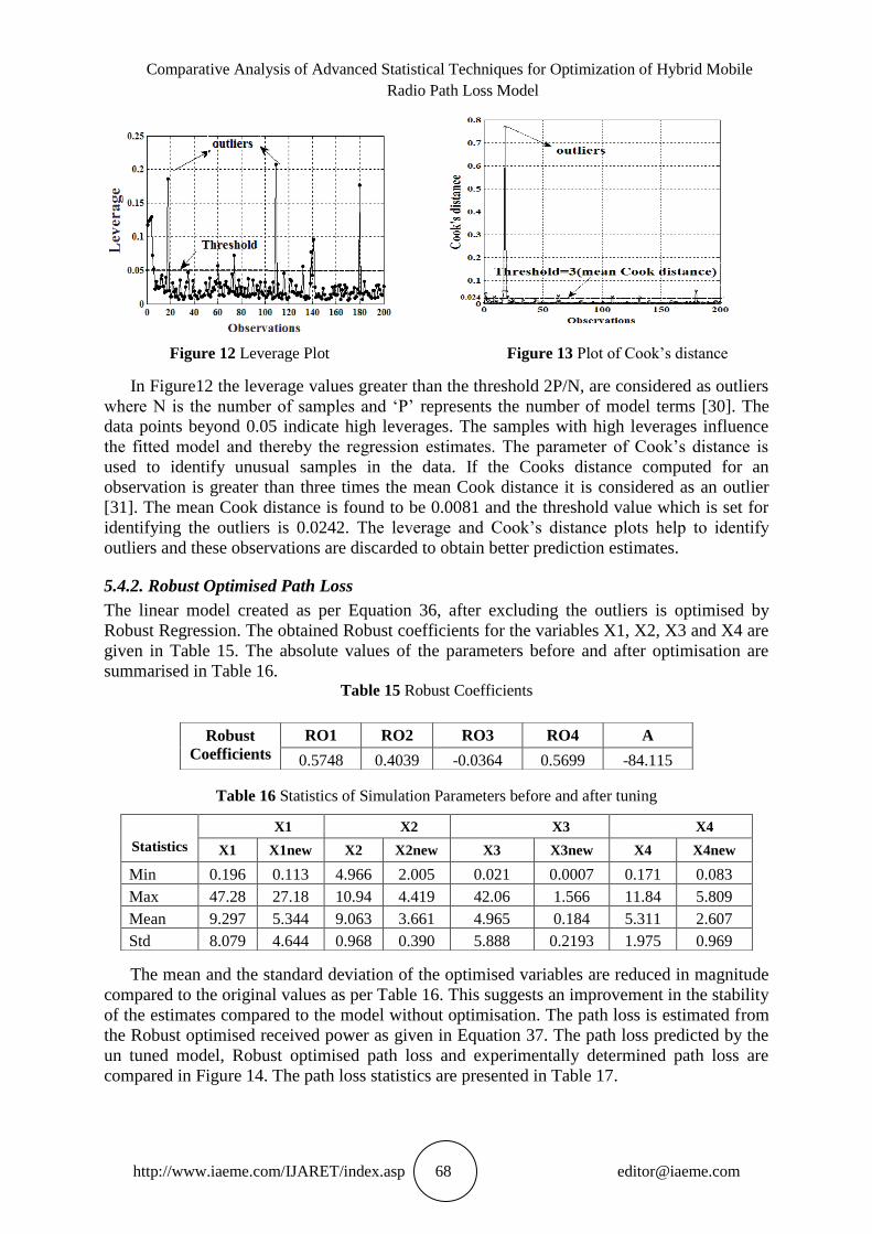
the leverages and cook distances. The plots of cook‟s distance and leverage with respect to

number of samples are shown in Figures 12 and 13.




Figure 12 Leverage Plot Figure 13 Plot of Cook‟s distance

In Figure12 the leverage values greater than the threshold 2P/N, are considered as outliers

where N is the number of samples and „P‟ represents the number of model terms [30]. The

data points beyond 0.05 indicate high leverages. The samples with high leverages influence

the fitted model and thereby the regression estimates. The parameter of Cook‟s distance is

used to identify unusual samples in the data. If the Cooks distance computed for an

observation is greater than three times the mean Cook distance it is considered as an outlier

[31]. The mean Cook distance is found to be 0.0081 and the threshold value which is set for

identifying the outliers is 0.0242. The leverage and Cook‟s distance plots help to identify

outliers and these observations are discarded to obtain better prediction estimates.

5.4.2. Robust Optimised Path Loss

The linear model created as per Equation 36, after excluding the outliers is optimised by

Robust Regression. The obtained Robust coefficients for the variables X1, X2, X3 and X4 are

given in Table 15. The absolute values of the parameters before and after optimisation are

summarised in Table 16. Table 15 Robust Coefficients

Table 16 Statistics of Simulation Parameters before and after tuning

The mean and the standard deviation of the optimised variables are reduced in magnitude

compared to the original values as per Table 16. This suggests an improvement in the stability

of the estimates compared to the model without optimisation. The path loss is estimated from

the Robust optimised received power as given in Equation 37. The path loss predicted by the

un tuned model, Robust optimised path loss and experimentally determined path loss are

compared in Figure 14. The path loss statistics are presented in Table 17.

Robust

Coefficients

RO1 RO2 RO3 RO4 A

0.5748 0.4039 -0.0364 0.5699 -84.115

Statistics

X1 X2 X3 X4


Min 0.196 0.113 4.966 2.005 0.021 0.0007 0.171 0.083

Max 47.28 27.18 10.94 4.419 42.06 1.566 11.84 5.809

Mean 9.297 5.344 9.063 3.661 4.965 0.184 5.311 2.607

Std 8.079 4.644 0.968 0.390 5.888 0.2193 1.975 0.969



Figure 14 Robust optimised Path Loss

Table 17 Path Loss Comparison

From Table 17, it is found that the average path loss estimated by the Robust optimised

model is 128 db which varies from the measured path loss by 2.3 db as compared to 3.9db of

the hybrid WI model prior to optimisation. The optimised result has a good agreement with

the measured data. There is an improvement of 1.6 db as a result of optimisation, and the

variance is reduced compared to the hybrid WI model. The improvement in the prediction

result is due to the identification and removal of outliers before performing the optimisation

by Robust regression.

5.5. Comparison of the Optimised Path Loss models

The optimisation is performed by Multiple Linear Regression and advanced statistical

techniques of Ridge and Robust Regression. The average path loss values predicted from the

optimised models at respective distances are summarised in Table 18.

Table 18 Path Loss Comparison

The model predicted mean path losses from Table 18 are compared with the average path

loss obtained from measurements (125.7 db). It is observed that the path loss estimated by the

Ridge optimized model has the best performance. It has a much closer agreement to the

Path Loss

Models

Path Loss (db)

Min Max Mean


Hybrid W-I (un tuned) 70 138 121.8

Robust optimised 99 137 128

Distance

(kms)

Model Predicted Path Loss (db)

Hybrid W-I

model

Optimised Path Loss

MLR Ridge Robust

0.5260 97.7010 105.4698 115.3125 113.0813

1.012 114.9644 119.6452 124.5484 125.6129

1.599 124.8332 123.0493 128.1521 129.9986

2.077 130.7233 127.5641 130.6667 131.9744

2.527 128.9605 129.0444 132.6111 133.3556

2.880 133.7102 130.1101 133.1143 134.0714

Mean PL 121.8154 122.6137 127.4008 128.0157




measured path loss, than the predictions made by MLR optimized and Robust optimized

models. The results of advanced statistical methods of Ridge and Robust regressions are

almost comparable. In order to validate the results, various error statistics are computed and

are summarised in Table 19.

Table 19 Performance Comparison in terms of Error Metrics

The error metrics quantitatively validate the use of Ridge Regression as the best suited

optimization method for the data under consideration. From Table 19 it is found that, the error

values are reduced for the optimized models compared to the hybrid WI model without

tuning. It is observed that the Prediction Error (PE), MSE, RMSE and other error metrics are

least for the Ridge optimized model. The advanced statistical method of Ridge Regression has

a best performance, since it uses biased estimates as compared to the unbiased estimators of

Multiple Linear Regression. This ensures the prediction of more stable and more reliable

values. The results justify the suitability and efficiency of using Ridge regression in the

context of optimising the mobile radio path loss. A plot of an overall path loss comparison is

shown in Figure 15.

Figure 15 Overall Path Loss Comparisons

5.6. Comparison of Goodness of Fit for the Optimisation Techniques

The improvement in the prediction results can be attributed to the model parameters modified

by optimization. Goodness of fit tests is performed on the model parameters X1, X2, X3 and

X4 to assess the performance before and after optimization. The parameters are fit linearly

and the Goodness of Fit Tests are done using curve fitting tool in Matlab. The major

Goodness of Fit (GOF) statistics of Sum Square Error (SSE) and RMSE are compared for the

original and optimized parameters in the three optimization techniques. The comparison of

GOF statistics are summarized in Table 20.

Error statistics Hybrid W-I

model (db)

Optimised PL models

MLR Robust Ridge

Prediction Error (PE) 3.0945 2.9788 2.6679 1.1701

Mean Square Error (MSE) 0.0479 0.0444 0.0356 0.0068

Root Mean Square Error(RMSE) 0.2188 0.2106 0.1886 0.0827

Spread Corrected (SC) RMSE 0.6433 0.6192 0.5546 0.2432

Standard deviation of Error (SD) 0.2177 0.2096 0.1877 0.0823

Relative Error (%) (RE) 3.1901 3.0711 2.7501 1.2100



Table 20 Comparison of Goodness of Fit Statistics for the parameters

From the Table 20 it is observed that all the optimized parameters have lesser values of

RMSE and Sum Squares of Error (SSE) compared to the original values. The parameters of

Robust optimized model have an improvement compared to MLR. The Ridge optimized

parameters has the least metrics of SSE and RMSE as compared to MLR and Robust

optimised values. The results justify that the Ridge optimized path loss model improves the

prediction compared to MLR and Robust optimised models. Figure 16 shows the linear fit for

the parameters X1, X2, X3 and X4 optimized by Ridge regression.

Figure 16 Linear Fit of the parameters for Ridge Optimised model

The three optimized path loss models are fit linearly and are their performances are

compared in terms of GOF statistics as shown in Table 21.

Table 21 Overall comparisons of GOF Statistics for the optimisation Techniques

In Table 21, it is found that SSE and RMSE values are least for optimization performed

by Ridge regression as compared to Multiple Linear Regressions and Robust results.

Although MLR provides better predictions compared to simple linear regressions, the

estimates are unbiased. The predictions in MLR may not be accurate and the high variance of

Parameter

s

SSE RMSE

Original

Values

Optimised new Values Original

Value

Optimised new Values

MLR Robust Ridge MLR Robust Ridge

X1 5504 2182 1819 1267 5.272 3.319 3.031 2.53

X2 186.2 125 30.37 27.97 0.969 0.794 0.391 0.375

X3 9365 1305 13.88 7.735 6.877 2.567 0.2647 0.197

X4 778.8 360.1 187.6 140 1.983 1.349 0.9734 0.840

Statistics

Optimisation Techniques

MLR Robust Ridge

SSE 7365 1794 1681

R-squared 0.6232 0.7749 0.8245

Adjusted R-Squared 0.6213 0.7738 0.8236

Root Mean Squared Error 6.0990 3.0100 2.9131




the coefficients reduces the precision of estimation. In Robust optimization, the unusual data

that affects the estimates is identified and eliminated. Hence Robust regression provides an

improvement in the values of SSE and RMSE compared to MLR. The measure R- square and

Adjusted R-Squared has the highest value for the Ridge optimized model, followed by Robust

and MLR optimizations. The larger value suggests a better fit with the data and justifies the

purpose of optimization in the context of improving the prediction results. Comparing the

statistical tuning techniques it can be concluded that for the data under analysis, the

optimization performed by Ridge regression is most suitable to obtain accurate path loss

predictions.

6. CONCLUSIONS

The work presented in the paper aims at optimizing the semi deterministic hybrid mobile

radio model to improve the path loss prediction. The statistical techniques are implemented

for tuning the propagation model. In this process, optimized path loss models are developed

using Multiple Linear Regression, Ridge and Robust regression. The performances of the

optimized models are evaluated by error metrics and Goodness of Fit tests. The results

indicate that the prediction error is 1.1701 for Ridge optimized model, 2.6679 for Robust

optimized model and 2.9788 for MLR optimized model. The error metrics are least for the

path loss predictions made by Ridge optimized model compared to MLR and Robust

optimized models. The results of Goodness of Fit tests also justify the efficient performance

of the Ridge optimized path loss model in achieving the best prediction results. As an

extension, further optimization techniques can be implemented to check their feasibility and

improve the prediction results.

REFERENCES

[1] Parsons, J.D., (2000). The mobile radio propagation channel. Wiley.

[2] Klozar, L. and Prokopec, J., (2011) April,‟ Propagation path loss models for mobile

communication‟.In Radioelektronika (RADIOELEKTRONIKA), 2011 21st International

Conference IEEE pp. 1-4.

[3] Akhoondzadeh-Asl, L. and Noori, N., (2007), December. Modification and tuning of the

universal okumura-hata model for radio wave propagation predictions. In Microwave

Conference, 2007. APMC 2007. Asia-Pacific IEEE pp. 1-4.

[4] Priya, T.S., (2010). Optimised COST-231 Hata models for WiMAX path loss prediction

in suburban and open urban environments. Modern Applied Science, 4(9), p.75.

[5] Dalela, C., Prasad, M.V.S.N. and Dalela, P.K., (2012). Tuning of COST-231 Hata model

for radio wave propagation predictions. Academy & Industry Research Collaboration

Center.

[6] Mousa, A., Najjar, M. and Alsayeh, B., (2013). Path Loss Model Tuning at GSM 900 for a

Single Cell Base Station. International Journal of Mobile Computing and Multimedia

Communications (IJMCMC), 5(1), pp.47-56.

[7] Tahat, A. and Taha, M., (2012), November. Statistical tuning of Walfisch-Ikegami

propagation model using particle swarm optimization. In Communications and Vehicular

Technology in the Benelux (SCVT), 2012 IEEE 19th Symposium on (pp. 1-6). IEEE.

[8] Ambroziak, S.J. and Katulski, R.J., (2014) April. Statistical tuning of walfisch-ikegami

model for the untypical environment. In Antennas and Propagation (EuCAP), 2014 8th

European Conference IEEE pp. 2087-2091.

[9] Ambawade, D., Karia, D., Potdar, T., Lande, B.K., Daruwala, R.D. and Shah, A., (2010)

May. Statistical tuning of Walfisch-Ikegami model in urban and suburban environments.

In Mathematical/Analytical Modelling and Computer Simulation (AMS), 2010 Fourth

Asia International Conference IEEE pp. 538-543.



[10] Bhuvaneshwari, A., Hemalatha, R. and Satyasavithri, T.,( 2016). Semi Deterministic

Hybrid Model for Path Loss Prediction Improvement. Procedia Computer Science, (92),

pp.336-344.

[11] NCSS Statistical Software. Chapter 335: Ridge Regression. NCSS, LLC. All Rights

reserved.

[12] Costa, J.C., (2008). Analysis and optimization of empirical path Loss models and

shadowing effects for the Tampa Bay Area in the 2.6 GHz Band.

[13] Joseph, I. and Konyeha, C.C., (2013).Urban Area Path loss Propagation Prediction and

Optimisation Using Hata Model at 800MHz. IOSR Journal of Applied Physics (IOSR-

JAP), 3, pp.8-18.

[14] Brown, S.H.,(2009) Multiple linear regression analysis: a matrix approach with

MATLAB. Alabama Journal of Mathematics, 34, pp.1-3.

[15] Rollin Brant (2007) - “Multiple Linear Regressions”.

[16] El-Dereny, M. and Rashwan, N.I.,(2011). Solving multicollinearity problem using ridge

regression models. Int. J. Contemp. Math. Sciences, 6(12), pp.585-600.

[17] Uslu, V.R., Egrioglu, E. and Bas, E.,(2014). Finding Optimal Value for the Shrinkage

Parameter in Ridge Regression via Particle Swarm Optimization. American Journal of

Intelligent Systems, 4(4), pp.142-147.

[18] Hoerl, A.E. and Kennard, R.W.,(1970). Ridge regression: Biased estimation for non

orthogonal problems. Technometrics, 12(1), pp.55-67.

[19] Dalkilic, T.E., Kula, K.S. and Hanci, B.Y.,(2014). Path Loss Prediction by Robust

Regression Methods. Effects of Skewness on Three Span Reinforced Concrete T Girder

Bridges, pp.26-34.

[20] Peter J. Huber and Elvezio M. Ronchetti (2009) "Robust Statistics”, second edition John

Wiley & Sons, Inc., publication.

[21] Schumacker, R.E., Monahan, M.P. and Mount, R.E., (2002). A comparison of OLS and

robust regression using S-PLUS. Multiple Linear Regression Viewpoints, 28(2), pp.10-13.

[22] Faruk, N., Ayeni, A. and Adediran, Y.A., (2013). On the study of empirical path loss

models for accurate prediction of TV signal for secondary users. Progress In

Electromagnetics Research B, 49, pp.155-176.

[23] https://www.mathworks.com/help/curvefit/evaluating-goodness-of-fit.html

[24] Bhuvaneshwari, A., Hemalatha, R. and Satyasavithri, T., (2013), November. Development

of an empirical power model and path loss investigations for dense urban region in

Southern India. In Communications (MICC), 2013 IEEE Malaysia International

Conference IEEE pp. 500-505.

[25] Lee, W.C., (1985). Estimate of local average power of a mobile radio signal. IEEE

Transactions on Vehicular Technology, 34(1), pp.22-27.

[26] Vinod, H.D. and Ullah, A., (1981). Recent advances in regression methods Vol. 41.

Marcel Dekker Incorporated.

[27] http://support.minitab.com/en-us/minitab/17/topic-library/modeling-statistics/regression-

and-correlation/model-assumptions/what-is-a-variance-inflation-factor-vif/

[28] http://www.mathworks.com/help/econ/collintest.html#btcdtr4.

[29] Cule, E., Vineis, P. and De Iorio, M., (2011). Significance testing in ridge regression for

genetic data. BMC bioinformatics, 12(1), p.372.

[30] https://in.mathworks.com/help/stats/linearmodel.plotdiagnostics.html

[31] http://in.mathworks.com/help/stats/cooks-dis.




AUTHORS DETAILS

A. Bhuvaneshwari, obtained her B.E degree in the field of Electronics and

Communication Engineering (E.C.E), and M. Tech degree with specialization

in Digital Systems and Computer Electronics (D.S.C.E) from Jawaharlal

Nehru Technological University Hyderabad (J.N.T.U.H). She is currently

working as an Associate Professor in Deccan College of Engineering and

Technology (DCET), Hyderabad. She has 17 years of teaching experience.

She is pursuing the Ph.D degree from J.N.T.U.H. Her research interests

include Mobile Communication, Wireless networks, and Image processing.

Dr. Hemalatha Rallapalli, is in the department of Electronics and

Communication Engineering at University college of Engineering, Osmania

University, Hyderabad. She has 20 years of teaching experience. She has

obtained her B.Tech degree from Sri Krishna Deva Raya University,

Ananthapur, Andhra Pradesh, in 1992, her M. Tech degree in Embedded

systems and Ph.D in wireless communication (Cognitive Radio) from

Jawaharlal Nehru Technological University, Hyderabad. She has various

publications to her credit in International conferences and Journals. She is a

member of IEEE and IETE, and her research interests include Wireless

communication, Embedded Systems and Global Positioning System.

Dr. T. Satya Savithri, is presently working as Professor in ECE Department

of JNTUH College of Engineering, Hyderabad. Her research interests include,

Digital Image Processing, Design and Testing of VLSI and also Wireless

communications. She has 38 publications in various national and International

Journals and Conferences. She has 20 years of teaching experience. She has

obtained her B. Tech degree from NIT Warangal, M.E from Osmania and

PhD in Digital Image Processing from JNTU Hyderabad. Presently, she is

guiding 8 students at Ph.D. level.

Simulation Parameters Values

Transmitted power 40 dBm

Transmitted frequency( MHz) 947.5

Length of the buildings (xt) 15 m

Height of the building(hroof) 15m

Separation between the buildings (s) 10m

Street width (w) 20

Receiver height (m) 1.5

Transmitter Height 30-70m

Diffraction loss factor (ka) 54

Cable Loss 3 dB

Distance factor(kd) 18

Frequency factor (kf) -3.9830

Distance power loss Coefficient 33

Propagation constant 19.8444

Permittivity value of floor 7

Reflection coefficient of the ground -0.3656

Reflection coefficient of the wall 0.1667

Optimum Incident angle ( ) 30

COMPARATIVE ANALYSIS OF ADVANCED · PDF fileof optimizing the mobile radio path loss model is...

Documents

Transcript of COMPARATIVE ANALYSIS OF ADVANCED · PDF fileof optimizing the mobile radio path loss model is...