Simple Indoor Path Loss Prediction Algorithm and ...

Noname manuscript No.(will be inserted by the editor)

Simple Indoor Path Loss Prediction Algorithm and

Validation in Living Lab Setting

David Plets · Wout Joseph ·

Kris Vanhecke · Emmeric Tanghe ·

Luc Martens

Received: date / Accepted: date

Abstract A simple heuristic algorithm has been developed for an accurateprediction of indoor wireless coverage, aiming to improve existing models uponmultiple aspects. Extensive measurements on several floors in four buildingsare used as validation cases and show an excellent agreement with the pre-dictions. As the prediction is based on the free-space loss model for everyenvironment, it is generally applicable, while other propagation models areoften too dependent on the environment upon which it is based. The appli-cability of the algorithm to a wireless testbed network in a living lab settingwith WLAN 802.11b/g nodes is investigated by a site survey. The results canbe extremely useful for the rollout of indoor wireless networks.

Keywords indoor propagation · WLAN · algorithm · prediction

1 Introduction

The increasing use of indoor wireless systems, such as WLAN (Wireless LocalArea Network) (broadcast) systems in e.g., conference rooms, office build-ings,. . . or sensor networks [1] for network management, monitoring, secu-rity,. . . gives rise to a need for propagation prediction algorithms that canbe used for different building types (office buildings, exhibition halls, facto-ries,. . . ), with a sufficient accuracy. The characterization of indoor propagationand path loss in indoor environments has been the subject of extensive researchand many models have been proposed to make accurate predictions [2–26]. Dif-ferent prediction approaches have been followed.

David Plets, Wout Joseph, Kris Vanhecke, Emmeric Tanghe, Luc MartensGhent University / IBBT, Dept. of Information TechnologyGaston Crommenlaan 8 box 201, B-9050 Ghent, BelgiumFax: +32 9 33 14899E-mail: [email protected]

2 David Plets et al.

Statistical (site-specific) one-slope models [15–23] (e.g. multi-wall models) pre-dict path loss based on measurements of a specific site or for a specific environ-ment. They are easy to construct when a lot of measurement data is availableand allow a fast prediction. However, the validity of the prediction is mostlylimited to the propagation environment it represents. In order to obtain a reli-able prediction model for a new building type (or a new transmitter location),an additional measurement campaign will most likely have to be executed.In [15,27], indoor path losses have been statistically investigated for differ-ent room categories (adjacent to transmitter room, non-adjacent,. . . ) in 14houses. Path loss in five office environments has been determined and the im-portance of taking wall attenuations into account in the prediction model isindicated in [16]. In [18], low prediction errors are obtained, but the analy-sis was performed for a site-specific validation of the ITU Indoor Path Lossmodel (only indoor office environments), whereas our algorithm is generallyapplicable (office environment, exhibition hall, retirement centre,. . . ). In [20],different propagation models were tuned to a measurement set, but unlike inthis paper, no validation measurements were performed. Tuning a predictionmodel can be understood as adapting the model parameters to make the pre-dictions correspond with the path loss measurements that were performed.Unlike in many other works, no parameter tuning will be executed in the val-idation phase of our prediction model.One-slope models and different multi-wall based models were analyzed andresults have been provided for a typical office environment in [28]. The stan-dard deviation of the model error was around 6 dB for the best model. In [21],a simple one-slope model was constructed for a mostly-LoS environment. Avalue of 2 for the path loss exponent n was obtained. LoS and NLoS measure-ments have been fitted to a one-slope model in [23]. The path loss exponenthere accounted also for the wall losses for the NLoS measurements. However,no model validations in other rooms or buildings were executed. In [22], a sta-tistical path loss model is proposed for different propagation conditions. Novalidation measurements have been performed to test the model.

To avoid the limited prediction validity of statistical models, ray-tracing andray-launching model techniques [2–6] take into account the geometry of thebuilding and the used materials. They usually require a vector based descrip-tion of the environment to identify the reflected and diffracted rays from sur-face and edges [29]. Although ray-tracing solvers claim to be accurate, theresults appear to be very dependent on geometrical details of the ground plan,which force the user to work with very accurate plans [30]. Moreover, theprediction transmission settings (number of interactions (transmissions, reflec-tions, and diffractions) of the rays with the environment) may have a relevantinfluence on the prediction results: differences up to 5 dB have been observedfor the average path loss along a line-of-sight (LoS) path when the number ofinteractions is adapted [31]. Finally, for large buildings, prediction times canrun into several hours.In [2], ray-tracing is used for indoor path loss prediction, with a distinction

Simple Indoor Path Loss Prediction Algorithm and Validation 3

between LoS and NLoS. Procentual prediction errors range from 5% to 10%,which is higher than for our prediction. Different ray-tracing approaches (field-sum and power-sum) have been investigated in [5]. Field-sum appeared to bemost accurate. In [3,4], efficient two-dimensional ray-tracing algorithms for anindoor environment have been presented, resulting in a significant reductionin the computational time, without losing prediction accuracy.

Numerical solver models [7–10] consist of screen or integral methods, Finite-difference time-domain (FDTD),. . . [29]. Numerical solvers also have the dis-advantage of a long calculation time, and the large dependence of the resultson the precision of the ground plan. Also, the dielectric material properties ofthe environment have to be accurately known to obtain a good prediction.A theoretical waveguide model permitting a rigorous modal solution is pro-posed for predicting path loss inside buildings in [7].

Our prediction algorithm can be classified as a heuristic algorithm. Heuris-tic predictions [11–14] are based on one or more rules of thumb in order tomake a path loss prediction.Heuristic approaches have been proposed in [12–14]. An indoor propagationmodel making use of the estimation of the transmitted field at the corners ofeach room is presented in [12]. Good results (mean absolute prediction errorof 2.2 dB) are obtained, but the model is less suitable for environments wherediffraction is the dominant mechanism. A more complex version of the domi-nant path loss model (using more model parameters) is studied and calibratedin order to minimise the prediction errors for a certain building in [13]. In [14],a WLAN planning tool was developed to optimize the position and number ofaccess points, as well as the total cost of the required equipment, according todifferent WLAN suppliers, in indoor and outdoor environments.The heuristic indoor path loss prediction model we are presenting is bothsimple and quick (as the statistical models), but will also prove to be very ac-curate (as numerical and ray-tracing solvers claim to be), although no tuningof the model will be performed in the model validation phase. Furthermore, ourmodel is also valid for different building types. The proposed algorithm avoidsthe quoted problems of the statistical and ray-tracing methods by determiningthe dominant path between transmitter and receiver [11,32]. Compared to [11,32], adaptations such as path loss model simplification, the avoidance of neuralnetworks, and a physically intuitive approach are carried out. The simplifiedapproach is proposed without losing prediction accuracy: the obtained devia-tions are lower than only 3 dB. A measurement campaign has been executedon several floors in four buildings in Belgium for construction and extensivevalidation of the propagation model. As our algorithm is based on free-spaceloss for every environment, the algorithm is generally applicable, while otherpredictions are often too dependent on the environment upon which the usedpropagation model is based. The applicability of the algorithm to a wirelessliving lab with WLAN 802.11b/g nodes is investigated by a site survey. Weaim to provide an physically intuitive, yet accurate prediction of the path loss


for different types of public and office buildings. The prediction algorithm canbe of great interest to anyone who wants to set up a WLAN, sensor, or broad-cast network in either home or professional environments [33].

Section 2 describes the investigated buildings and their use in the propagationmodeling procedure. In Section 3, the measurement setup is described, andin Section 4, the prediction algorithm is presented. The modeling of the pathloss parameters is discussed in Section 5 and Section 6 investigates differentvalidation cases. In Section 7, the applicability of the model to a wireless livinglab is discussed. Finally, conclusions are presented in Section 8.

2 Investigated buildings

In this paper, an indoor path loss model for the 2.4 GHz-band will be formu-lated. To determine the model parameters, PL measurements and simulationshave been performed in four very different buildings, named Zuiderpoort (I),De Vijvers (II), Lamot (III), and Vooruit (IV). The characteristics of the in-vestigated buildings are described hereafter and are summarized in Table 1 atthe end of this section.

Zuiderpoort is a modern three-storey office building, with movable walls(layered drywalls) around a core consisting of concrete walls (Table 1). Fig. 1shows the third floor of this building. Path loss measurements have beenperformed on both floors (1,581 path loss samples on the second floor and5,078 samples on the third floor). The orange walls are layered drywalls, thegrey ones are made of concrete. In order to assure the validity of the predic-tions for the entire building floor, trajectories T1-T5 are chosen to representLoS, obstructed line-of-sight (OLoS), as well as NLoS propagation cases, whilerooms A-H are chosen to investigate propagation through subsequently adja-cent rooms. In rooms A-H, an average path loss in the room is calculated bymoving the receiver antenna randomly through the room during 2 minutes.For the measurements on the third floor (Fig. 1), TA is the access point formeasurement trajectories T1-T5 and TB for measurements in rooms A-H andfor measurement trajectory ’corr’ (corridor).

Fig. 1 Measurement trajectories on the third floor of the Zuiderpoort office building. Thepoints for which the different path loss contributions are investigated in Table 3 are circledon T1, T3, T4, and in rooms E and F.


De Vijvers is a retirement home (Table 1), where 7,095 measurementsamples were collected along twelve trajectories (T1 - T12) on the ground floor(see Fig. 2). The building mainly consists of concrete walls. Both LoS and NLoStrajectories are chosen to investigate the path loss prediction. Trajectory T12is a part of trajectory T1, but for T1, TA was the active transmitter, whereasfor all other trajectories (T2-T12), TB was active.

Fig. 2 Ground plan of ’De Vijvers’ with indication of transmitters TA and TB and themeasurement trajectories T1-T12. The points for which the different path loss contributionsare investigated in Table 3 are indicated on T3, T4, and T6 with a black dot within a whitedot.

Lamot is a multi-storey congress and heritage centre with multipurposerooms for conferences, seminars, workshops, fashion shows, product presen-tations,... Thirteen path loss measurement trajectories (4,070 samples) havebeen executed on the third floor and the fifth floor, both having a similargeometry. The building is mainly constructed with concrete walls. Both LoSand NLoS trajectories are chosen to investigate the path loss prediction.

Vooruit is a polyvalent arts centre for all kinds of events (concerts, par-


ties, debates, . . . ), built between 1911 and 1914. Measurements are performedon three floors (ground floor, first floor, and second floor). This building alsomainly consists of concrete walls, some of them even with a thickness of 50 cm.Seventeen trajectories (4,390 samples) have been traversed for the path lossmeasurements in this building. Mostly NLoS predictions are chosen to inves-tigate the path loss prediction.It is clear that these buildings have very different characteristics. It will beshown that our approach is capable to predict path loss for these differentindoor environments.

ID name and dominant measured goal

description materials floors

I Zuiderpoort layered 2nd PL measurement (tuning)

(office building) drywall, 3rd PL measurement (validation)

concrete

II De Vijvers concrete ground floor PL measurement

(retirement home) (validation+interaction loss tuning)

III Lamot concrete 3rd PL measurement (validation)

(congress centre) 5th PL measurement (validation)

IV Vooruit concrete, ground floor PL measurement (validation)

(arts centre) glass 1st PL measurement (validation)

2nd PL measurement (validation)

Table 1 Overview of the characteristics of the investigated buildings.

3 Path loss measurements

The path loss prediction models incorporated in the prediction algorithm arebased upon, and validated with path loss measurements in different buildings.This section discusses the setup for these path loss measurements and theirreproducibility.

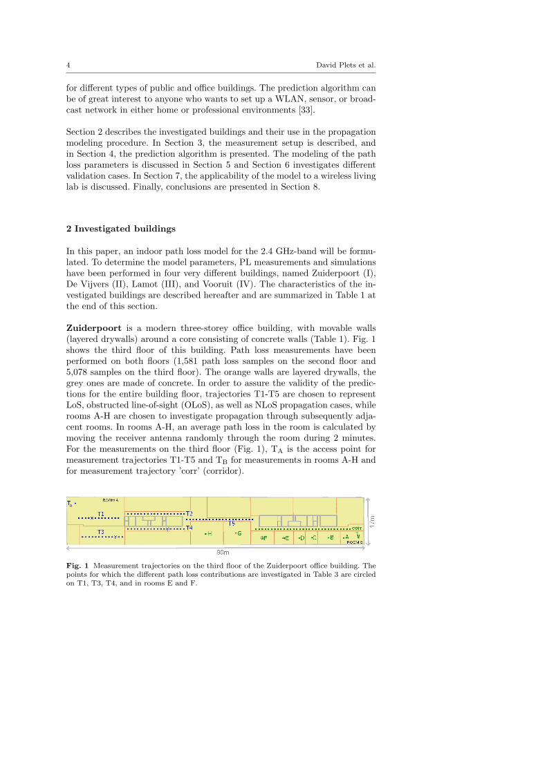
As Tx an omnidirectional Jaybeam antenna type MA431Z00 with a gain of4.2 dBi is used [34]. The Tx is placed at a height of 2.5 m above ground level(typical access point height in public environments). It is fed with a continu-ous sine wave at 2.4 GHz (ISM-band, typical for WLAN communication) withan EIRP of 20 dBm. Possible interfering sources (e.g., WiFi networks) aredesactivated in order not to influence the measurements. The receiver antenna(identical to Tx) is attached to a cart at a height of 1 m (typical user deviceheight) and is connected to a Rohde & Schwarz FSEM30 spectrum analyzerwith a frequency range from 20 Hz up to 26.5 GHz. The output of the SA issampled and stored on a laptop used to record and process the measurementdata. Fig. 3 shows the measurement setup.


Fig. 3 Measurement setup.

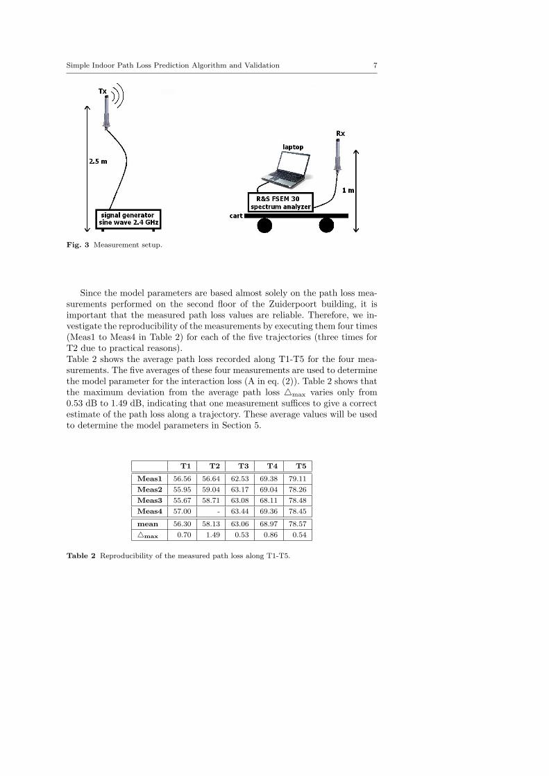
Since the model parameters are based almost solely on the path loss mea-surements performed on the second floor of the Zuiderpoort building, it isimportant that the measured path loss values are reliable. Therefore, we in-vestigate the reproducibility of the measurements by executing them four times(Meas1 to Meas4 in Table 2) for each of the five trajectories (three times forT2 due to practical reasons).Table 2 shows the average path loss recorded along T1-T5 for the four mea-surements. The five averages of these four measurements are used to determinethe model parameter for the interaction loss (A in eq. (2)). Table 2 shows thatthe maximum deviation from the average path loss △max varies only from0.53 dB to 1.49 dB, indicating that one measurement suffices to give a correctestimate of the path loss along a trajectory. These average values will be usedto determine the model parameters in Section 5.

T1 T2 T3 T4 T5

Meas1 56.56 56.64 62.53 69.38 79.11

Meas2 55.95 59.04 63.17 69.04 78.26

Meas3 55.67 58.71 63.08 68.11 78.48

Meas4 57.00 - 63.44 69.36 78.45

mean 56.30 58.13 63.06 68.97 78.57

△max 0.70 1.49 0.53 0.86 0.54

Table 2 Reproducibility of the measured path loss along T1-T5.


4 Algorithm concept and implementation

In this section, the concept and the implementation of the prediction algo-rithm is discussed. Our goal is to develop an accurate and fast algorithm thatdoes not make use of extensive fitting to obtain good predictions, as this oftenleads to results which are only usable for the investigated building.The planning algorithm predicts the indoor coverage by means of a path loss(PL) prediction based on the Indoor Dominant Path Model (IDP) [11,32].This model is a compromise between semi-empirical models only consider-ing the ”direct” ray between transmitter Tx and receiver Rx (e.g., multi-wallmodel) and ray-tracing models where hundreds of rays and their interactionswith the environment are investigated. In the IDP model, propagation focuseson the dominant path between transmitter and receiver, i.e., the path alongwhich the signal encounters the smallest obstruction in terms of path loss.It takes into account the length along the path, the number and type of in-teractions (e.g., reflection, transmission, etc.), the material properties of theobjects encountered along the path, etc. The approach of using the IDP modelis justified by the fact that more than 95% of the energy received is containedin only 2 or 3 rays [11]. According to [11], predictions made by IDP modelsreach the accuracy of ray-tracing models or even exceed it.

4.1 Comparison with the IDP model

Different propagation properties can be chosen to be included into the IDPmodel. We have chosen to take into account the distance along the dominantpath (distance loss), the corresponding wall losses, and the propagation di-rection changes along the dominant path (interaction loss). The IDP modelas presented in [32] also adds other factors, such as waveguiding, transmitterroom size,. . . The more factors used though, the more tuning is needed (lim-ited general use) and the more difficult it is to determine the influence of eachsingle factor on the path loss. As a result, neural networks are mostly neededto construct a path loss model. Also, the more influencing factors included,the higher the dimensions of the problem, and the more training patternsneeded to construct reliable models. Moreover, unlike with neural networks,these contributions are physically in line with the actual path loss caused bythe three factors, which makes it easier to a posteriori adapt e.g., penetra-tion losses based on new measurements or add new wall types to the pathloss model. Therefore, we aimed to construct a model as simple as possible,but as complex as necessary for accurate predictions, this way improving theIDP model from [11,32]. In Sections 5 and 6, it will be demonstrated that theproposed three contributing factors suffice to perform solid predictions.


4.2 General path loss model

The path loss model, based on the three discussed contributions (distance loss,cumulated wall loss, interaction loss), will now be discussed. Path losses aredetermined between the transmit antenna of an access point and a receivingantenna at a certain location. The total path loss for a path between an accesspoint in one room and a receiver location in another room, is the sum of thethe distance loss along the path, the total wall loss along the path, and theinteraction loss along the path. The total path loss of a certain path can thusbe calculated as follows:

PL = PL0 + 10 n log(d

d0)

︸︷︷︸

distance loss

+∑

i

LWi

︸︷︷︸

cumulated wall loss

+∑

j

LBj

︸︷︷︸

interaction loss

, (1)

where PL [dB] is the total path loss along the path, PL0 [dB] is the pathloss at a distance of d0 according to the distance loss model, d [m] is thedistance along the path between access point and receiver, d0 [m] is a referencedistance, and n [-] is the path loss exponent. d0 was chosen 1 m here. Thefirst two terms of the sum represent the path loss due to the distance alongthe considered path, noted here as the ”distance loss”. It is calculated for acertain path as the path loss at a distance equal to the length of the path

that traverses all the walls of the considered path.∑

i

LWiis the ”cumulated

wall loss” along the path (i.e., the sum of the wall losses LWiof all walls Wi

traversed along the path, i = 1,. . ., W, where W is the total number of walls

along the path).∑

j

LBjis the ”interaction loss”, i.e. the cumulated loss LBj

caused by all propagation direction changes Bj of the propagation path fromaccess point to receiver, with j = 1,. . ., B, where B is the number of timesthe propagation path changes its direction. The dominant path is definedas the path for which the sum of the cumulated wall loss, the distance loss,and the interaction loss is the lowest. Values for the model parameters will bedetermined in Section 5. Typical contributions of the distance loss, cumulatedwall loss, and interactions loss for different transmitter-receiver configuratonswill be presented in Section 4.3.

4.3 Judiciously chosen and physically intuitive path

Our model was aimed at an intuitive understanding of how path loss is af-fected, without losing accuracy. The three contributions taken into account inthe model of equation (1) (distance loss, cumulated wall loss, and interactionloss) are selected based on the real physical propagation of a wave betweentransmitter and receiver.


To gain more insight into the model, we will now investigate the contribu-tions to the total path loss of the three factors, for eight different transmitter-receiver configurations: five points circled in Fig. 1, and three points indicatedwith a black dot within a white dot in Fig. 2 in the building of De Vijvers(retirement home in Ghent, Belgium, see Section 2). Table 3 shows the threedifferent contributions to the total path loss for each of these points PB

T, whereB indicates the building where the point is located (Z = Zuiderpoort or V = DeVijvers) and T indicates the trajectory on which or the room in which thepoint is located. This table also shows the dominant path from transmitterto receiver. Different propagation situations are illustrated: LoS (PZ

T1), OLoS(obstructed line-of-sight) with one (PZ

T3) or more (PZE) walls between Tx and

Rx, and propagation through corridors and/or rooms (all other points). In allcases, the distance loss is by far the most dominant factor. As the cumulatedwall loss increases, it becomes more likely that another path (through corri-dors) will be dominant. In the De Vijvers building (containing a lot of concretewalls), the interaction losses can be quite high (up to 17.2 dB for PV

T4).Our model was aimed at an intuitive understanding of how path loss is affected,without losing accuracy.

Rx Tx DL CWL IL PL Dominant path

point [dB] [dB] [dB] [dB]

PZ

T1TA 57.0 0 0 57.0 direct ray

PZ

T3TA 64.1 2.0 0 66.1 direct ray

PZ

T4TA 69.5 4.0 1.9 75.4 through room of PZ

T3

PZ

ETB 67.4 8.0 0 75.4 direct ray

PZ

FTB 70.0 6.0 3.0 79.0 through corridor and room of PZ

E

PV

T3TB 75.2 2.0 17.0 94.2 through corridors along T2 and T3

PV

T4TB 78.7 2.0 17.2 97.9 through corridors along T2, T3, and T4

PV

T6TB 73.8 6.0 15.0 94.8 through corridor along T2,

then crossing the inner yard

Table 3 Overview of the three different contributions (DL = Distance Loss, CWL = Cu-mulated Wall Loss, IL = Interaction Loss) to the total path loss PL between eight receiverpoints and the transmitter in two buildings.

5 Modeling the parameters of the dominant path model

In this section, the model parameters will be determined. The four build-ings described in Section 2 are used for the construction and the validationof the path loss model. We have deliberately chosen different types of build-ings (modern office building, retirement home, modern congress centre withlarge exhibition halls, and old arts centre), in order to investigate the generalapplicability of the model. Path loss measurements on the different investi-


gated building floors are used either for tuning the model parameters or forvalidation purposes (see Table 1, column ’goal’).

5.1 Distance loss

A first limitation we impose ourselves is the use of the free-space loss modelfor the distance loss (see equation (1): n = 2, PL0 = 40 dB, d0 = 1 m),because we aim to use a general model, avoiding fitting and tuning of themodel to agree with existing measurement data of a certain environment. Thisway, we intend to increase the general applicability of equation (1). Changingthese parameters might probably improve the prediction accuracy in the modeltuning phase, but it is more likely that the resulting model would be toospecific for a specific building (type), something we try to avoid in this research.The free-space loss model seemed like a good starting point for a generalprediction model. Results will indicate that this was a feasible choice.

5.2 Cumulated wall loss

For the determination of the term representing the cumulated wall loss (seeequation (1), we have first measured the penetration loss of the two wall typespresent in the Zuiderpoort building, layered drywalls (orange walls in Fig. 1)and concrete walls (grey walls in Fig. 1), and we have used the (rounded)values in the model, 2 dB and 10 dB respectively. For other wall types, wehave based the loss values on available literature. For glass (windows or glassdoors), 2 dB was used [35]. The importance of correct wall penetration lossvalues is demonstrated in [29]. A distinction was made between thin (< 15 cm)and thick (> 15 cm) walls. For thick concrete walls a loss of 15 dB [36] was used.The model’s penetration loss database can easily be extended with penetrationlosses for various other materials using numbers and tables of [35–37].

5.3 Interaction loss

Based on the contribution of the distance loss and wall loss factor obtained asexplained above, the value of the third factor, the interaction loss factor (seeequation (1)), was adjusted in order to match the predictions to measurementsperformed on the second floor of the Zuiderpoort building. The measurementson this building floor were thus used to tune the model (see Table 1, column’goal’) and allowed us to determine the relation between the angle made bya propagation path and the additional loss associated with the propagationdirection change. Because the interaction loss should be the same for e.g., threechanges of 30◦ and one change of 90◦, a linear relationship is proposed.

LBj= A · B̂j (2)


where LBj[dB] is the loss caused by bend Bj, A [dB/◦] is a parameter de-

pending on the dominant material in the building and B̂j [◦] is the anglecorresponding with bend Bj. Based on measurements in two perpendicularcorridors, A was determined at 0.0556 dB/◦ or 5 dB/90◦ for the Zuiderpoort(see Fig. 1) building, consisting mainly of layered drywalls.

5.4 Parameter values for the buildings used for validation

With the model parameters for distance loss, cumulated wall loss, and in-teraction loss now fixed, measurements on the third floor of the Zuiderpoortbuilding were performed as a first validation without any further tuning (seeTable 1), albeit in a very similar environment.However, for the De Vijvers building, an environment mainly consisting ofconcrete walls (vs. the lighter layered drywalls in the Zuiderpoort building),the loss when propagating around corners appeared to be higher than for theZuiderpoort building. The interaction loss for this environment was tuned toa value of 0.1946 dB/◦ or 17.5 dB/90◦ for concrete walls. In fact, it was onlytuned for one of the twelve trajectories (T5, a trajectory where the dominantpath made a propagation direction change), so all other measured trajectoriesin this building can be considered as validation trajectories as well (see Ta-ble 1, column ’goal’).For the remaining two buildings (Lamot and Vooruit), all model parametersfrom the analysis of the Zuiderpoort and De Vijvers buildings were used un-changed. Both buildings mainly consist of concrete, so we could immediatelyuse the interaction loss function from the De Vijvers building, and validate themodel with new measurements, without any additional tuning. Sections 5.5and 6 will demonstrate that these validation results are more than satisfac-tory. Table 1 summarizes the goal (model tuning and/or validation) of themeasurements in the different buildings.

5.5 Model performance for second floor of Zuiderpoort building

The model of eq. (1) with its parameters chosen as explained above is nowused to calculate the deviations between the algorithm predictions and themeasurements for the second floor of the Zuiderpoort building.Table 4 shows for all trajectories on the second floor (used for modeling) andthird floor (used for validation) the measured average path loss PLms [dB], thepredicted path loss PLpr, and the deviation δ [dB] for the considered modelfor Tx and Rx at heights of 2.5 m and 1 m respectively. δ [dB] is defined asfollows.

δ[dB] = PLpr[dB] − PLms[dB] (3)

Small deviations are obtained in Table 4 for the Zuiderpoort building. Anaverage for the absolute value of the deviation |δ| is 1.77 dB for the second


floor. The deviation δ has an average of -1.15 dB with a standard deviationof 2.33 dB. Values for the standard deviation of 3 dB to 6 dB are consideredto be excellent according to [29]. Our prediction model performs much betterthan this requirement.

14 David Plets et al.PL

ms

PL

pr

δPL

ms

PL

pr

δPL

ms

PL

pr

δPL

ms

PL

pr

δ

[dB

][d

B]

[dB

][d

B]

[dB

][d

B]

[dB

][d

B]

[dB

][d

B]

[dB

][d

B]

Zuid

erpoort

Vijvers

Lam

ot

Vooruit

T1(2)

56.3

61.1

-4.8

T1

66.6

66.7

-0.2

T1(3)

64.2

61.4

2.9

T1(0)

61.3

59.6

1.8

T2(2)

58.1

59.9

-1.8

T2

68.8

68.8

0.0

T2(3)

65.2

64.1

1.1

T2(0)

73.4

67.0

6.4

T3(2)

63.1

62.8

0.3

T3

91.3

92.0

-0.7

T3(3)

63.4

62.7

0.8

T3(0)

77.5

78.0

-0.4

T4(2)

69.0

67.7

1.3

T4

96.9

97.0

-0.1

T4(3)

64.1

61.2

2.9

T4(0)

82.8

80.3

2.5

T5(2)

78.6

79.3

-0.7

T5

83.4

83.4

0.0

T5(3)

74.4

74.5

-0.1

T5(0)

60.8

57.8

3.0

A50.3

53.3

-3.0

T6

99.3

96.7

2.6

T6(3)

87.1

85.7

1.4

T6(0)

77.0

76.4

0.7

B61.7

61.4

0.3

T7

84.5

82.0

2.4

T7(3)

83.1

80.2

2.8

T7(0)

81.7

78.2

3.5

C64.1

67.4

-3.3

T8

97.6

99.7

-2.1

T1(5)

60.4

60.4

0.0

T1(1)

71.8

67.0

4.8

D65.9

71.3

-5.4

T9

100.6

95.5

5.1

T2(5)

63.1

63.9

-0.8

T2(1)

68.8

72.1

-3.3

E68.6

75.4

-6.8

T10

96.2

91.7

4.5

T3(5)

62.9

62.1

0.8

T1(2)

74.4

74.1

0.4

F79.6

79.0

0.6

T11

70.4

67.8

2.5

T4(5)

61.1

60.1

1.1

T2(2)

71.1

66.1

5.0

G82.3

78.6

3.7

T12

64.4

63.8

0.6

T6(5)

87.4

85.5

1.9

T3(2)

67.9

63.5

4.4

H84.9

81.8

3.1

T7(5)

79.0

79.1

-0.2

T4(2)

83.1

78.7

4.4

corr

66.9

66.9

0.0

T5(2)

86.2

83.0

3.3

T1(3)

58.1

59.1

-1.0

T6(2)

69.9

65.4

4.4

T2(3)

70.1

70.2

-0.1

T7(2)

66.1

62.4

3.7

T3(3)

65.5

65.2

0.3

T8(2)

71.3

71.7

-0.4

T4(3)

78.9

73.5

5.4

T5(3)

79.7

76.9

2.8

|δ| a

vg

δavg

σ|δ| a

vg

δavg

σ|δ| a

vg

δavg

σ|δ| a

vg

δavg

σ

ZP

(2)

1.7

7-1

.15

2.3

3V

ijvers

1.7

31.2

22.1

9Lam

ot

1.2

91.1

21.2

3Vooruit

3.0

82.6

02.4

9

ZP

(3)

2.5

6-0

.24

3.4

7

Table

4M

easu

red

aver

age

path

loss

PL

ms

[dB

]alo

ng

diff

eren

ttr

aje

ctori

es,pre

dic

ted

aver

age

path

loss

PL

pr

[dB

]and

thei

rdev

iations

δ[d

B]fr

om

PL

ms

info

ur

buildin

gs

(buildin

gfloor

isin

dic

ate

dbet

wee

nbra

cket

sfo

rtr

aje

ctori

esw

ith

the

sam

enam

e).A

ver

age

abso

lute

dev

iations|δ| a

vg,aver

age

dev

iations

δa

vg,

and

standard

dev

iation

σof

the

dev

iations

δ(s

eeeq

.(3

))in

dic

ate

din

bold

(num

ber

bet

wee

nbra

cket

sin

dic

ate

sbuildin

gfloor,

ZP

=Zuid

erpoort

).


6 Validation of path loss model with measurements in other

buildings

The parameter values of our prediction model are based on measurements onone floor of one building (second floor, Zuiderpoort, see Section 5). In this sec-tion, we validate the general applicability of the path loss model constructedin Section 5, by comparing with measurements on another floor of the Zuider-poort building, but also in the three other buildings presented in Section 2.Table 4 summarizes for trajectories in all buildings the measured average pathloss PLms [dB], the predicted path loss PLpr [dB], and the deviation δ [dB] =PLpr - PLms for the considered model for Tx and Rx at heights of 2.5 m and1 m respectively. It also gives a summary of the average absolute deviations|δ|avg, the average deviations δavg, and standard deviation σ of the deviationsfor each of the buildings.The measurement trajectories on the third floor of the Zuiderpoort build-

ing (see Fig. 1) serve as a first validation for the model proposed in Section 5(based on measurements on second floor of Zuiderpoort building). The lowdeviations (|δ| = 2.56 dB, δ = -0.24 dB, σ = 3.47 dB) show that the obtainedprediction model is valid for a similar propagation environment (same build-ing, but other floor, similar materials used) without tuning of the parametersin contrary to e.g., [38].The measurement campaign of twelve trajectories on the ground floor in ’De

Vijvers’ (see Fig. 2), a retirement home, has been considered as a secondvalidation case. Table 4 shows that the predictions match the measurementsexcellently (|δ| = 1.73 dB, δ = 1.22 dB, σ = 2.19 dB). The deviations are smallespecially for the trajectories with the lowest path losses (T1, T2, T11, T12are LoS or OLoS) which will be most relevant for actual networks (locationson trajectories with PL > 90 dB will probably have no WiFi reception).The measurement campaign of thirteen trajectories on the third and fifth floorin congress centre ’Lamot’ has been considered as a third validation case, andthe measurement campaign of seventeen trajectories on three floors of arts cen-tre ’Vooruit’ as a fourth validation case. Just like for ’De Vijvers’, predictionsare very accurate (see Table 4), indicating that the proposed model is also validfor environments for which the model has not been tuned.Table 4 shows the accuracy of our propagation prediction, even for buildingswhere no tuning at all has been performed (Lamot and Vooruit). In e.g.,[11],the obtained deviations are similar, but there, δ was considered, while weused |δ|, which is more correct. Moreover, the values in [11] were obtained fora similar environment, whereas we have investigated different environments,indicating the improvement compared to [11].

7 Applicability to a wireless network in a living lab setting

In this section, it is investigated if the propagation model can be used topredict the path loss at the locations of the (fixed) nodes of a wireless (video)


living lab. The testbed network and the setup for the performed measurementswill be presented, followed by an investigation of the prediction quality.

7.1 Living lab network

34 WLAN nodes have been put up at a height of 2.5 m in different rooms on thethird floor of the Zuiderpoort office building in Ghent, Belgium (see Section 2).Fig. 4 shows the location of all WLAN nodes on this floor (90 m x 17 m).The nodes are Alix 3C3 devices running Linux. These are embedded PC’sequipped with a Compex 802.11b/g WLM series MiniPCI network adapter.The wireless network interface is connected to a vertically polarized quarter-wavelength omnidirectional dipole antenna with a gain of 3 dBi. An 802.11bsignal is transmitted by node 31 (indictated with circle in Figure 4) with apower of 0 dBm at a data rate of 1 Mbps. In total, 9000 packets are broadcastat a rate of 10 packets/s. In this validation procedure, all other nodes arereceiving nodes measuring the Received Signal Strength Indication (RSSI).This RSSI value is then converted to a received power, based on a calibrationperformed in our lab. While space variability will inevitably be present due tothe fixed character of the nodes (see also [39]), this procedure at least allowsto average out the time variability present in the UHF band [40].

Fig. 4 Living lab node locations on third floor of Zuiderpoort building (transmitter locatedroughly in middle of building floor, indicated with circle).

7.2 Results

Path loss measurements with the spectrum analyser are executed close tothese node locations (distance less than 30 cm). These obtained PL values arecompared with the algorithm prediction and with the path loss values PLlab

measured by the nodes themselves (see Section 7.2). Nodes in the same roomor nodes close to each other will also be investigated as a group as shownin Fig. 4 in order to obtain an averaged value, since the node locations aresubject to small-scale fading mechanisms, which are not taken into account inthe algorithm.

Fig. 5 shows the path loss PL2.5 mpred predicted by our algorithm and the path


loss PLSA measured by the spectrum analyzer, as a function of the path lossPLlab measured by the nodes for the different node groups. Perfect agreementis represented by the full line. Table 5 shows the mean deviations δmean andstandard deviations σ between the SA measurement, prediction, and nodemeasurements. Table 5 shows that the mean deviations vary between -0.27and -2.14 dB when all nodes are considered separately, with standard devi-ations between 4.72 and 6.96 dB. When nodes are grouped, both the meandeviations (maximum of 1.56 dB) and the standard deviations (maximum of4.65 dB) are lower (see Fig. 5 and Table 5).In general, the predictions have a good correspondence with the node mea-surements. The mean deviation approaches 0 dB and the standard deviationcorresponds with common shadowing margins. A first reason for the exist-ing deviations is indeed the influence of fading mechanisms. Since in total,we only dispose of 33 measurements executed at one point location, it is im-possible to average out the small-scale fading for each zone (most consideredgroups consist of only 2 to 4 locations, see Fig. 4). This is probably also whythe predictions have lower deviations than the SA measurements, probablybecause the prediction is based on an average path loss in an area, while theSA measurements are more subject to fading mechanisms. Secondly, the pathloss close to the transmitter (low path losses) is somewhat overestimated bythe propagation model (see also T1(2) in Table 4, column ’Zuiderpoort’). Thephenomenon of received powers being higher than expected close to the trans-mitter is also reported in [41].We can thus conclude that it is possible to predict path losses for WLANnodes in a living lab network.

Fig. 5 Comparison of path loss measured by living lab nodes with path loss measuredwith spectrum analyser (SA) and with path loss predicted by propagation model for nodesgrouped as in Fig. 4.


Separate nodes Grouped nodes

δmean [dB] σ [dB] δmean [dB] σ [dB]

PL2.5 mpred

- PLSA -1.87 6.96 -1.56 4.37

PLlab - PLSA -2.14 6.81 -0.99 4.65

PLlab - PL2.5 mpred

-0.27 4.72 0.57 4.34

Table 5 Mean deviations δmean and standard deviations σ of the different predictions andmeasurements for the wireless living lab network.

8 Conclusions

A simple heuristic indoor path loss prediction algorithm for the 2.4 GHz-bandhas been developed. It bases its calculations on the dominant path betweentransmitter and receiver, but increases simplicity, introduces a strictly phys-ical approach, and avoids neural networks and the accompanying need for alot of training patterns. The algorithm, concept, and physical rationale havebeen presented. Measurements have been executed to construct and validatethe model, on different floors of four buildings of different types. In contrary tomany existing models no tuning of the model parameters is performed for thevalidation. Still, excellent correspondence between measurements and predic-tions is obtained: average absolute deviations for the different buildings varybetween 1.29 dB and 3.08 dB, with standard deviations below 3.5 dB. Thealgorithm allows to quickly set up a new WLAN network for different types ofindoor environments. The algorithm has also been applied to a WLAN livinglab network with (fixed) nodes at specific locations. The average deviationsremain low, but due to small-scale fading mechanisms, standard deviationsincrease up to around (maximally) 7 dB.Future research could include an extension of the prediction algorithm forpropagation through floors or ceilings and the development of an algorithmfor automatic network optimization.

Acknowledgements This work was supported by the IBBT−DEUS project, co-fundedby the IBBT (Interdisciplinary institute for BroadBand Technology), a research institutefounded by the Flemish Government in 2004, and the involved companies and institutions.W. Joseph is a Post-Doctoral Fellow of the FWO-V (Research Foundation - Flanders).

References

1. N. R. Prasad and M. Alam, “Security Framework for Wireless Sensor Networks,” Wire-less Personal Communications, vol. 37, no. 3-4, pp. 455–469, 2006.

2. S. Hamzah, M. Baharudin, N. Shah, Z. Abidin, and A. Ubin, “Indoor channel predictionand measurement for wireless local area network (WLAN) system,” in CommunicationTechnology, 2006. ICCT ’06. International Conference on, Guilin, China, November2006, pp. 1–4.


3. Zhong Ji and Bin-Hong Li and Hao-Xing Wang and Hsing-Yi Chen and T.K. Sarkar,“Efficient ray-tracing methods for propagation prediction for indoor wireless communi-cations,” IEEE Antennas and Propagation Magazine, vol. 43, no. 2, April.

4. Zhong Ji and Bin-Hong Li and Hao-Xing Wang and Hsing-Yi Chen and Yaw-Gen Zhau,“A new indoor ray-tracing propagation prediction model,” in Computational Electro-magnetics and Its Applications, 1999. Proceedings. (ICCEA ’99) 1999 InternationalConference on, 1999, pp. 540–542.

5. Yinghua Li and Zhengwei Du and Ke Gong, “Comparison of different calculating meth-ods for path loss in ray-tracing method at 2GHz,” in Microwave and Millimeter WaveTechnology, 2004. ICMMT 4th International Conference on, Proceedings, 18 - 21 Au-gust 2004, pp. 182–184.

6. M. D. R.P. Torres, L. Valle and M. Diez, “CINDOOR: an engineering tool for planningand design of wireless systems in enclosed spaces,” IEEE Antennas and PropagationMagazine, vol. 41, no. 4, pp. 11–22, 1999.

7. G.M. Whitman and Kyu-Sung Kim and E. Niver, “A theoretical model for radio signalattenuation inside buildings,” IEEE Transactions on Vehicular Technology, vol. 44,August 1995.

8. G. de la Roche, P. Flipo, Z. Lai, G. Villemaud, J. Zhang and J.-M. Gorce, “Combinationof Geometric and Finite Difference Models for Radio Wave Propagation in Outdoorto Indoor Scenarios,” in 3rd European Conference on Antennas and Propagation,Barcelona, Spain, 12-16 April 2010.

9. L. Nagy, “Comparison and Application of FDTD and Ray Optical Method for IndoorWave Propagation Modeling,” in 3rd European Conference on Antennas and Propaga-tion, Barcelona, Spain, 12-16 April 2010.

10. J. Moreno Delgado, M. Domingo Gracia, J. Basterrechea Verdeja, J.R. Perez Lopez andL. Valle Lopez, “Automatic Channel and Aps Allocation in WiFi Networks Using RayTracing Techniques and Particle Swarm Optimization,” in 3rd European Conference onAntennas and Propagation, Barcelona, Spain, 12-16 April 2010.

11. G. Wlfle, R. Wahl, P. Wertz, P. Wildbolz, and F. Landstorfer, “Dominant path pre-diction model for indoor scenarios,” in German Microwave Conference (GeMIC), Ulm,Germany, April 2005.

12. A.G. Dimitriou and S. Siachalou and A. Bletsas and J.N. Sahalos, “An Efficient Prop-agation Model for Automatic Planning of Indoor Wireless Networks,” in 3rd EuropeanConference on Antennas and Propagation, Barcelona, Spain, 12-16 April 2010.

13. M.B. Khrouf and M. Ayadi and S. Ben Romdhane and N. Saghrouni and S. Tabbaneand Z. Belhadj, “Indoor Prediction of Propagation Using Dominant Path: Study andCalibration,” in Electronics, Circuits and Systems, 2005. ICECS 2005. 12th IEEE In-ternational Conference on, Gammarth, December 2005.

14. P. Sebastiao, R. Tome, F. Velez, A. Grilo, F. Cercas, D. Robalo, A. Rodrigues, F. F.Varela and C. X. P. Nunes, “WLAN Planning Tool: a Techno-Economic Perspective,”in COST 2100 TD(09)935 meeting, Vienna, Austria, 28-30 September 2009.

15. D. Plets, W. Joseph, L. Verloock, E. Tanghe, and L. Martens, “Evaluation of IndoorPenetration Loss and Floor Loss for a DVB-H Signal at 514 MHz,” in 2010 IEEE In-ternational Symposium on Broadband Multimedia Systems and Broadcasting, Shangai,March 2010, paper No. mm2010-04.

16. S. Todd and M. El-Tanany and G. Kalivas and S. Mahmoud, “Indoor radio path losscomparison between the 1.7 GHz and 37 GHz bands,” in Universal Personal Commu-nications, 1993. Personal Communications: Gateway to the 21st Century. ConferenceRecord., 2nd International Conference on, vol. 2, Ottawa, Ont., October 1993, pp. 621–625.

17. S. Phaiboon, “An empirically based path loss model for indoor wireless channels inlaboratory building,” in TENCON ’02. Proceedings. 2002 IEEE Region 10 Conferenceon Computers, Communications, Control and Power Engineering, vol. 2, October 2002,pp. 1020–1023.

18. T. Chrysikos and G. Georgopoulos and S. Kotsopoulos, “Site-specific validation of ITUindoor path loss model at 2.4 GHz,” in World of Wireless, Mobile and MultimediaNetworks and Workshops, 2009. WoWMoM 2009. IEEE International Symposium ona, Kos, 15-19 June 2009, pp. 1–6.


19. A. Durantini and D. Cassioli, “A multi-wall path loss model for indoor UWB propa-gation,” Vehicular Technology Conference, 2005. VTC 2005-Spring. 2005 IEEE 61st,vol. 1, pp. 30–34, 30 May - 1 June 2005.

20. R.S. de Souza and R.D. Lins, “A new propagation model for 2.4 GHz wireless LAN,” inCommunications, 2008. APCC 2008. 14th Asia-Pacific Conference on, Tokyo, Japan,14-16 October 2008, pp. 1–5.

21. G.J.M. Janssen and R. Prasad, “Propagation measurements in an indoor radio environ-ment at 2.4 GHz, 4.75 GHz and 11.5 GHz,” Vehicular Technology Conference, 1992,IEEE 42nd, vol. 2, pp. 617–620, 10 May - 13 May 1992.

22. C. Perez-Vega and J.L. Garcia, “A Simple Approach to a Statistical Path Loss Modelfor Indoor Communications,” in Microwave Conference, 1997. 27th European, vol. 1,Jerusalem, Israel, 8 - 12 September 1997, pp. 617–623.

23. Jae-Woo Lim and Yong-Sub Shin and Jong-Gwan Yook, “Experimental performanceanalysis of IEEE802.11a/b operating at 2.4 and 5.3 GHz,” in Communications, 2004and the 5th International Symposium on Multi-Dimensional Mobile CommunicationsProceedings. The 2004 Joint Conference of the 10th Asia-Pacific Conference on, vol. 1,29 August - 1 September 2004, pp. 133–136.

24. S. Phaiboon and P. Phokharatkul and S. Somkuarnpanit and S. Boonpiyathud, “Upper-and lower-bound path-loss modeling for indoor line-of-sight environments,” in Mi-crowave Conference Proceedings, 2005. APMC 2005. Asia-Pacific Conference Proceed-ings, vol. 4, 4-7 December 2005.

25. J. Jemai and R. Piesiewicz and T. Kurner, “Calibration of an indoor radio propagationprediction model at 2.4 GHz by measurements of the IEEE 802.11b preamble,” inVehicular Technology Conference, 2005. VTC 2005-Spring. 2005 IEEE 61st, vol. 1,30 May - 1 June 2005, pp. 111–115.

26. R. Tahri and V. Guillet and J.Y. Thiriet and P. Pajusco, “Measurements and CalibrationMethod for WLAN Indoor Path Loss Modelling,” in 3G and Beyond, 2005 6th IEEInternational Conference on, 7-9 November 2005, pp. 1–4.

27. W. Joseph, L. Verloock, D. Plets, E. Tanghe, and L. Martens, “Characterization ofcoverage and indoor penetration loss of DVB-H signal of indoor gap filler in UHF band,”IEEE Transactions on Broadcasting, vol. 55, no. 3, pp. 589–597, 2009.

28. F. Capulli and C. Monti and M. Vari and F. Mazzenga, “Path Loss Models for IEEE802.11a Wireless Local Area Networks,” in Wireless Communication Systems, 2006.ISWCS ’06. 3rd International Symposium on, Valencia, Spain, 6-8 September 2006, pp.621–624.

29. J.-F. Wagen, “Indoor Service Coverage Predictions: How Good is Good enough?” in3rd European Conference on Antennas and Propagation, Barcelona, Spain, 12-16 April2010.

30. L. Stola, G. Urso, and P. Tenani, “Indoor propagation: Experimental validation at 1.7GHz of a UTD-based approach,” Wireless Personal Communications, vol. 3, no. 3, pp.225–241, 1996.

31. D. Plets, W. Joseph, K. Vanhecke, E. Tanghe, and L. Martens, “Development of anAccurate Tool for Path Loss and Coverage Prediction in Indoor Environments,” inEuropean Conference on Antennas and Propagation 2010, Barcelona, 12-16 April 2010.

32. G. Wlfle, F. Landstorfer, R. Gahleitner, and E. Bonek, “Extensions to the field strengthprediction technique based on dominant paths between transmitter and receiver in in-door wireless communications,” 1997.

33. G. Berger, R. Goedeken, and J. Richardson, “Motivation and Implementation of aSoftware H.264 Real-Time CIF Encoder for Mobile TV Broadcast Applications,” IEEETransactions on Broadcasting, vol. 53, no. 2.

34. Mat Equipement, “MA431Z00, 2400..2485 MHz, 4 dBi,” Tech. Rep. [Online]. Available:http://www.gigacomp.ch/pdfs/MatJaybeam MA431Z00.pdf

35. Y. E. Mohammed, A. Abdallah, and Y. A. Liu, “Characterization of Indoor PenetrationLoss At ISM Band,” in Asia-Pasific Conference on Environmental ElectromagneticsCEEM’2003, Hangzhou, China, Nov. 2003, pp. 25– 28.

36. Y. Zhang and Y. Hwang, “Measurements of the characteristics of indoor penetrationloss,” in Vehicular Technology Conference, 1994 IEEE 44th, vol. 3, Stockholm, Sweden,Jun. 1994, pp. 1741–1744.


37. G. Tesserault and N. Malhouroux and P. Pajusco, “Determination of Material Char-acteristics for Optimizing WLAN Radio,” in Wireless Technologies, 2007 EuropeanConference on, Munich, Germany, 8-10 October 2007, pp. 225–228.

38. A. Turkmani and A. de Toledo, “Modelling of radio transmissions into, and withinbuildings at 900, 1800 and 2300 MHz,” IEE Proceedings, vol. 140, no. 6, pp. 462–470,Dec. 1993.

39. N. Papadakis, A. Economou, J. Fotinopoulou, and P. Constantinou, “Radio PropagationMeasurements and Modeling of Indoor Channels at 1800 MHz,” Wireless PersonalCommunications, vol. 9, no. 2, pp. 95–111, 1999.

40. A. Martinez, D. Zabala, I. Pena, P. Angueira, M. Velez, A. Arrinda, D. de la Vega, andJ. Ordiales, “Analysis of the DVB-T Signal Variation for Indoor Portable Reception,”IEEE Transactions on Broadcasting, vol. 55, no. 1, pp. 11–19, March 2009.

41. G. Steinbock, T. Pedersen and B. H. Fleury, “Model for the Path Loss of In-roomReverberant Channels,” in COST 2100 TD(10)11057 meeting, Aalborg, Denmark, 2-4June 2010.

Simple Indoor Path Loss Prediction Algorithm and ...

Documents

Transcript of Simple Indoor Path Loss Prediction Algorithm and ...