Common Methodology Mistakes in Educational Research, Revisited, along with a Primer on Both
126
DOCUMENT RESUME ED 429 110 TM 029 652 AUTHOR Thompson, Bruce TITLE Common Methodology Mistakes in Educational Research, Revisited, along with a Primer on Both Effect Sizes and the Bootstrap. PUB DATE 1999-04-00 NOTE 126p.; Paper presented at the Annual Meeting of the American Educational Research Association (Montreal, Quebec, Canada, April 19-23, 1999). PUB TYPE Numerical/Quantitative Data (110) Reports - Descriptive (141) Speeches/Meeting Papers (150) EDRS PRICE MF01/PC06 Plus Postage. DESCRIPTORS *Analysis of Variance; *Educational Research; *Effect Size; *Research Methodology; Research Problems; *Statistical Significance; Tables (Data) IDENTIFIERS *Bootstrap Methods ABSTRACT As an extension of B. Thompson's 1998 invited address to the American Educational Research Association, this paper cites two additional common faux pas in research methodology and explores some research issues for the future. These two errors in methodology are the use of univariate analyses in the presence of multiple outcome variables (with the converse use of univariate analyses in post hoc explorations of detected multivariate effects) and the conversion of intervally scaled predictor variables into nominally scaled data in the service of the "of variance" (OVA) analyses. Among the research issues to receive further attention in the future is the appropriate use of statistical significance tests. The use of the descriptive bootstrap and the various types of effect size from which the researcher should select when characterizing quantitative results are also discussed. The paper concludes with an exploration of the conditions necessary and sufficient for the realization of improved practices in educational research. Three appendixes contain the Statistical Package for the Social Sciences for Windows syntax used to analyze data for three tables. (Contains 16 tables, 15 figures, and 173 references.) (SLD) ******************************************************************************** * Reproductions supplied by EDRS are the best that can be made * * from the original document. * ********************************************************************************
Transcript of Common Methodology Mistakes in Educational Research, Revisited, along with a Primer on Both

DOCUMENT RESUME
ED 429 110 TM 029 652
AUTHOR Thompson, BruceTITLE Common Methodology Mistakes in Educational Research,
Revisited, along with a Primer on Both Effect Sizes and theBootstrap.
PUB DATE 1999-04-00NOTE 126p.; Paper presented at the Annual Meeting of the American
Educational Research Association (Montreal, Quebec, Canada,April 19-23, 1999).
PUB TYPE Numerical/Quantitative Data (110) Reports - Descriptive(141) Speeches/Meeting Papers (150)
EDRS PRICE MF01/PC06 Plus Postage.DESCRIPTORS *Analysis of Variance; *Educational Research; *Effect Size;
*Research Methodology; Research Problems; *StatisticalSignificance; Tables (Data)
IDENTIFIERS *Bootstrap Methods
ABSTRACTAs an extension of B. Thompson's 1998 invited address to the
American Educational Research Association, this paper cites two additionalcommon faux pas in research methodology and explores some research issues forthe future. These two errors in methodology are the use of univariateanalyses in the presence of multiple outcome variables (with the converse useof univariate analyses in post hoc explorations of detected multivariateeffects) and the conversion of intervally scaled predictor variables intonominally scaled data in the service of the "of variance" (OVA) analyses.Among the research issues to receive further attention in the future is theappropriate use of statistical significance tests. The use of the descriptivebootstrap and the various types of effect size from which the researchershould select when characterizing quantitative results are also discussed.The paper concludes with an exploration of the conditions necessary andsufficient for the realization of improved practices in educational research.Three appendixes contain the Statistical Package for the Social Sciences forWindows syntax used to analyze data for three tables. (Contains 16 tables, 15figures, and 173 references.) (SLD)
********************************************************************************* Reproductions supplied by EDRS are the best that can be made *
* from the original document. *
********************************************************************************

aeraad99.wp1 3/29/99
Common Methodology Mistakes in Educational Research, Revisited,
Along with a Primer on both Effect Sizes and the Bootstrap
Bruce Thompson
Texas A&M University 77843-4225and
Baylor College of Medicine
U.S. DEPARTMENT OF EDUCATIONOffice of Educational Research and improvement
EDUCATIONAL RESOURCES INFORMATIONCENTER (ERIC)
Erer-,:rdocument has been reproduced asreceived from the person or organizationoriginating it.
0 Minor changes have been made toimprove reproduction quality.
Points of view or opinions stated in thisdocument do not necessarily representofficial OERI position or policy. 1
PERMISSION TO REPRODUCE ANDDISSEMINATE THIS MATERIAL HAS
BEEN GRANTED BY
3_0,Lee, slIANO.501
TO THE EDUCATIONAL RESOURCESINFORMATION CENTER (ERIC)
Invited address presented at the annual meeting of theAmerican Educational Research Association (session #44.25),Montreal, April 22, 1999. Justin Levitov first introduced me to thebootstrap, for which I remain most grateful. I also appreciate the
C4 thoughtful comments of Cliff Lunneborg and Russell Thompson on aU, previous draft of this paper. The author and related reprints mayCID
CD be accessed through Internet URL: "http://acs.tamu.edu/-bbt6147/".04CD
2
BEST COPY AVAILABLE
0
Common Methodology Mistakes -2-Abstract
Abstract
The present AERA invited address was solicited to address the theme
for the 1999 annual meeting, "On the Threshold of the Millennium:
Challenges and Opportunities." The paper represents an extension of
my 1998 invited address, and cites two additional common
methodology faux pas to complement those enumerated in the previous
address. The remainder of these remarks are forward-looking. The
paper then considers (a) the proper role of statistical
significance tests in contemporary behavioral research, (b) the
utility of the descriptive bootstrap, especially as regards the use
of "modern" statistics, and (c) the various types of effect sizes
from which researchers should be expected to select in
characterizing quantitative results. The paper concludes with an
exploration of the conditions necessary and sufficient for the
realization of improved practices in educational research.
3

Common Methodology Mistakes -3-Introduction
In 1993, Carl Kaestle, prior to his term as President of the
National Academy of Education, published in the Educational
Researcher an article titled, "The Awful Reputation of Education
Research." It is noteworthy that the article took as a given the
conclusion that educational research suffers an awful reputation,
and rather than justifying this conclusion, Kaestle focused instead
on exploring the etiology of this reality. For example, Kaestle
(1993) noted that the education R&D community is seemingly in
perpetual disarray, and that there is a
...lack of consensus--lack of consensus on goals,
lack of consensus on research results, and lack of a
united front on funding priorities and
procedures.... [T]he lack of consensus on goals is
more than political; it is the result of a weak
field that cannot make tough decisions to do some
things and not others, so it does a little of
everything... (p. 29)
Although Kaestle (1993) did not find it necessary to provide a
warrant for his conclusion that educational research has an awful
reputation, others have directly addressed this concern.
The National Academy of Science evaluated educational research
generically, and found "methodologically weak research, trivial
studies, an infatuation with jargon, and a tendency toward fads
with a consequent fragmentation of effort" (Atkinson & Jackson,
1992, p. 20). Others also have argued that "too much of what we see
in print is seriously flawed" as regards research methods, and that
"much of the work in print ought not to be there" (Tuckman, 1990,
4

Common Methodology Mistakes -4-Introduction
p. 22). Gall, Borg and Gall (1996) concurred, noting that "the
quality of published studies in education and related disciplines
is, unfortunately, not high" (p. 151).
Indeed, empirical studies of published research involving
methodology experts as judges corroborate these impressions. For
example, Hall, Ward and Comer (1988) and Ward, Hall and Schramm
(1975) found that over 40% and over 60%, respectively, of published
research was seriously or completely flawed. Wandt (1967) and
Vockell and Asher (1974) reported similar results from their
empirical studies of the quality of published research.
Dissertations, too, have been examined, and have been found
methodologically wanting (cf. Thompson, 1988a, 1994a).
Researchers have also questioned the ecological validity of
both quantitative and qualitative educational studies. For example,
Elliot Eisner studied two volumes of the flagship journal of the
American Educational Research Association, the American Educational
Research Journal (AERJ). He reported that,
The median experimental treatment time for seven of
the 15 experimental studies that reported
experimental treatment time in Volume 18 of the AERJ
is 1 hour and 15 minutes. I suppose that we should
take some comfort in the fact that this represents a
66 percent increase over a 3-year period. In 1978
the median experimental treatment time per subject
was 45 minutes. (Eisner, 1983, p. 14)
Similarly, Fetterman (1982) studied major qualitative projects, and
reported that, "In one study, labeled fAn ethnographic study of...,
5
Common Methodology Mistakes -5-Introduction
observers were on site at only one point in time for five days. In
a(nother] national study purporting to be ethnographic, once-a-
week, on-site observations were made for 4 months" (p. 17)
None of this is to deny that educational research, whatever
its methodological and other limits, has influenced and informed
educational practice (cf. Gage, 1985; Travers, 1983). Even a
methodologically flawed study may still contribute something to our
understanding of educational phenomena. As Glass (1979) noted,
"Our research literature in education is not of the highest
quality, but I suspect that it is good enough on most topics" (p.
12).
However, as I pointed out in a 1998 AERA invited address, the
problem with methodologically flawed educational studies is that
these flaws are entirely gratuitous. I argued that
incorrect analyses arise from doctoral methodology
instruction that teaches research methods as series
of rotely-followed routines, as against thoughtful
elements of a reflective enterprise; from doctoral
curricula that seemingly have.less and less room for
quantitative statistics and measurement content,
even while our knowledge base in these areas is
burgeoning (Aiken, West, Sechrest, Reno, with
Roediger, Scarr, Kazdin & Sherman, 1990; Pedhazur &
Schmelkin, 1991, pp. 2-3); and, in some cases, from
an unfortunate atavistic impulse to somehow escape
responsibility for analytic decisions by justifying
choices, sans rationale, solely on the basis that
6

Common Methodology Mistakes -6-Introduction
the choices are common or traditional. (Thompson,
1998a, p. 4)
Such concerns have certainly been voiced by others. For
example, following the 1998 annual AERA meeting, one conference
attendee wrote AERA President Alan Schoenfeld to complain that
At [the 1998 annual meeting] we had a hard time
finding rigorous research that reported actual
conclusions. Perhaps we should rename the
association the American Educational Discussion
Association.... This is a serious problem. By
encouraging anything that passes for inquiry to be a
valid way of discovering answers to complex
questions, we support a culture of intuition and
artistry rather than building reliable research
bases and robust theories. Incidentally, theory was
even harder to find than good research. (Anonymous,
1998, p. 41)
Subsequently, Schoenfeld appointed a new AERA committee, the
Research Advisory Committee, which currently is chaired by Edmund
Gordon. The current members of the Committee are: Ann Brown, Gary
Fenstermacher, Eugene Garcia, Robert Glaser, James Greeno, Margaret
LeCompte, Richard Shavelson, Vanessa Siddle Walker, and Alan
Schoenfeld, ex officio, Lorrie Shepard, ex officio, and William
Russell, ex officio. The Committee is charged to strengthen the
research-related capacity of AERA and its members, coordinate its
activities with appropriate AERA programs, and be entrepreneurial
in nature. [In some respects, the AERA Research Advisory Committee
Common Methodology Mistakes -7-Introduction
has a mission similar to that of the APA Task Force on Statistical
Inference, which was appointed in 1996 (Azar, 1997; Shea, 1996).]
AERA President Alan Schoenfeld also appointed Geoffrey Saxe
the 1999 annual meeting program chair. Together, they then
described the theme for the AERA annual meeting in Montreal:
As we thought about possible themes for the upcoming
annual meeting, we were pressed by a sense of
timeliness and urgency. With regard to timeliness,
...the calendar year for the next annual meeting is
1999, the year that heralds the new millennium....
It's a propitious time to think about what we know,
what we need to know, and where we should be
heading. Thus, our overarching theme [for the 1999
annual meeting] is "On the Threshold of the
Millennium: Challenges and Opportunities."
There is also a sense of urgency. Like many
others, we see the field of education at a point of
critical choices--in some arenas, one might say
crises. (Saxe & Schoenfeld, 1998, p. 41)
The present paper was among those invited by various divisions to
address this theme, and is an extension of my 1998 AERA address
(Thompson, 1998a).
Purpose of the Present Paper
In my 1998 AERA invited address I advocated the improvement of
educational research via the eradication of five identified faux
pas:
(1) the use of stepwise methods;
8
Common Methodology Mistakes -8-Purpose of the Paper
(2) the failure to consider in result interpretation the context
specificity of analytic weights (e.g., regression beta
weights, factor pattern coefficients, discriminant function
coefficients, canonical function coefficients) that are part
of all parametric quantitative analyses;
(3) the failure to interpret both weights and structure
coefficients as part of result interpretation;
(4) the failure to recognize that reliability is a characteristic
of scores, and not of tests; and
(5) the incorrect interpretation of statistical significance and
the related failure to report and interpret the effect sizes
present in all quantitative analyses.
Two Additional Methodology Faux Pas
The present didactic essay elaborates two additional common
methodology errors to delineate a constellation of seven cardinal
sins of analytic research practice:
(6) the use of univariate analyses in the presence of multiple
outcomes variables, and the converse use of univariate
analyses in post hoc explorations of detected multivariate
effects; and
(7) the conversion of intervally-scaled predictor variables into
nominally-scaled data in service of OVA (i.e., ANOVA, ANCOVA,
MANOVA, MANCOVA) analyses.
However, the present paper is more than a further elaboration
of bad behaviors. Here the discussion of these two errors focuses
on driving home two important realizations that should undergird
best methodological practice:
9
Common Methodology Mistakes -9-Purpose of the Paper
1. All statistical analyses of scores on measured/observed
variables actually focus on correlational analyses of scores
on synthetic/latent variables derived by applying weights to
the observed variables; and
2. The researcher's fundamental task in deriving defensible
results is to employ an analytic model that matches the
researcher's (too often implicit) model of reality.
These two realization will provide a conceptual foundation for the
treatment in the remainder of the paper.
Focus on the Future: Improving Educational Research
Although the focus on common methodological faux pas has some
merit, in keeping with the theme of this 1999 annual meeting of
AERA, the present invited address then turns toward the
constructive portrayal of a brighter research future. Three issues
are addressed. First, the proper role of statistical significance
testing in future practice is explored. Second, the use of so-
called "internal replicability" analyses in the form of the
bootstrap is described. As part of this discussion some "modern"
statistics are briefly discussed. Third, the computation and
interpretation of effects sizes are described.
Other methods faux pas and other methods improvements might
both have been elaborated. However, the proposed changes would
result in considerable improvement in future educational research.
In my view, (a) informed use of statistical tests, (b) the more
frequent use of external and internal replicability analyses, and
especially (c) required reporting and interpretation of effect
sizes in all quantitative research are both necessary and
10

Common Methodology Mistakes -10-Purpose of the Paper
sufficient conditions for realizing improvements.
Essentials for Realizing Improvements
The essay ends by considering how fields move and what must be
done to realize these potential improvements. In my view, AERA must
exercise visible and coherent academic leadership if change is to
occur. To date, such leadership has not often been within the
organization's traditions.
Faux Pas #6: Univariate as Against Multivariate Analyses
Too often, educational researchers invoke a series of
univariate analyses (e.g., ANOVA, regression) to analyze multiple
dependent variable scores from a single sample of participants.
Conversely, too often researchers who correctly select a
multivariate analysis invoke univariate analyses post hoc in their
investigation of the origins of multivariate effects. Here it will
be demonstrated once again, using heuristic data to make the
discussion completely concrete, that in both cases these choices
may lead to serious interpretation errors.
The fundamental conceptual emphasis of this discussion, as
previously noted, is on making the point that:
1. All statistical analyses of scores on measured/observed
variables actually focus on correlational analyses of scores
on synthetic/latent variables derived by applying weights to
the observed variables.
Two small heuristic data sets are employed to illustrate the
relevant dynamics, respectively, for the univariate (i.e., single
dependent/outcome variable) and multivariate (i.e., multiple
outcome variables) cases.
11

Common Methodology Mistakes -11-Faux Pas #6: Multivariate vs Univariate
Univariate Case
Table 1 presents a heuristic data set involving scores on
three measured/observed variables: Y, Xl, and X2. These variables
are called "measured" (or "observed") because they are directly
measured, without any application of additive or multiplicative
weights, via rulers, scales, or psychometric tools.
INSERT TABLE 1 ABOUT HERE.
However, ALL parametric analyses apply weights to the
measured/observed variables to estimate scores for each person on
synthetic or latent variables. This is true notwithstanding the
fact that for some statistical analyses (e.g., ANOVA) the weights
are not printed by some statistical packages. As I have noted
elsewhere, the weights in different analyses
...are all analogous, but are given different names
in different analyses (e.g., beta weights in
regression, pattern coefficients in factor analysis,
discriminant function coefficients in discriminant
analysis, and canonical function coefficients in
canonical correlation analysis), mainly to obfuscate
the commonalities of [all] parametric methods, and
to confuse graduate students. (Thompson, 1992a, pp.
906-907)
The synthetic variables derived by applying weights to the measured
variables then become the focus of the statistical analyses.
The fact that all analyses are part on one single General
Linear Model (GLM) family is a fundamental foundational

Common Methodology Mistakes -12-Faux Pas #6: Multivariate vs Univariate
understanding essential (in my view) to the informed selection of
analytic methods. The seminal readings have been provided by Cohen
(1968) viz, the univariate case, by Knapp (1978) viz, the
multivariate case, and by Bagozzi, Fornell and Larcker (1981)
regarding the most general case of the GLM: structural equation
modeling. Related heuristic demonstrations of General Linear Model
dynamics have been offered by Fan (1996, 1997) and Thompson (1984,
1991, 1998a, in press-a).
In the multiple regression case, a given person's score on
the measured/observed variable Y. is estimated as the
synthetic/latent variable The predicted outcome score for a
given person equals = a + b1(X1.) + b2(X2.), which for these data,
as reported in Figure 1, equals -581.735382 + [1.301899 x X1] +
[0.862072 x X21]. For example, for person 1, Y1 = [1.301899 x 392]
+ [0.862072 x 573] = 422.58.
INSERT FIGURE 1 ABOUT HERE.
Some Noteworthy Revelations. The "ordinary least squares"
(OLS) estimation used in classical regression analysis optimizes
the fit in the sample of each Y. to each Yi score. Consequently, as
noted by Thompson (1992b), even if all the predictors are useless,A
the means of Y and Y will always be equal (here 500.25), and theA
mean of the e scores (ei = Yi - Y.) will always be zero. These
expectations are confirmed in the Table 1 results.
It is also worth noting that the sum of squares (i.e., the sum
of the squared deviations of each person's score from the mean) of
the Y scores (i.e., 167,218.50) computed in Table 1 matches the
13

Common Methodology Mistakes -13-Faux Pas #6: Multivariate vs Univariate
"regression" sum of squares (variously synonymously called
"explained," "model," "between," so as to confuse the graduate
students) reported in the Figure 1 SPSS output. Furthermore, the
sum of squares of the e scores reported in Table 1 (i.e.,
32,821.26) exactly matches the "residual" sum of squares (variously
called "error," "unexplained," and "residual") value reported in
the Figure 1 SPSS output.
It is especially noteworthy that the sum of squares explained
(i.e., 167,218.50) divided the sum of squares of the Y scores
(i.e., the sum of squares "total" = 167,218.50 + 32,821.26 =
200,039.75) tells us the proportion of the variance in the Y scores
that we can predict given knowledge of the X1 and the X2 scores.
For these data the proportion is 167,218.50 / 200,039.75 = .83593.
This formula is one of several formulas with which to compute the
uncorrected regression effect size, the multiple le.
Indeed, for the univariate case, because ALL analyses are
correlational, an r2 analog of this effect size can always be
computed, using this formula across analyses. However, in ANOVA,
for example, when we compute this effect size using this generic
formula, we call the result eta2 (n2; or synonymously the
correlation ratio [not the correlation coefficient!]), primarily to
confuse the graduate students.
Even More Important Revelations. Figure 2 presents the
correlation coefficients involving all possible pairs of the five
(three measured, two synthetic) variables. Several additional
revelations become obvious.
14
Common Methodology Mistakes -14-Faux Pas #6: Multivariate vs Univariate
INSERT FIGURE 2 ABOUT HERE.
A
First, note that the Y scores and the e scores are perfectly
uncorrelated. This will ALWAYS be the case, by definition, sinceA
the Y scores are the aspects of the Y scores that the predictors
can explain or predict, and the e scores are the aspects of the Y
scores that the predictors cannot explain or predict (i.e., becauseA
ei is defined as Y. - Y., therefore rywax, = 0). Similarly, the
measured predictor variables (here X1 and X2) always have
correlations of zero with the e scores, again because the e scores
by definition are the parts of the Y scores that the predictors
cannot explain.
Second, note that the ry,yma reported in Figure 3 (i.e.,
.9143) matches the multiple R reported in Figure 1 (i.e., .91429),
except for the arbitrary decision by different computer programs to
present these statistics to different numbers of decimal places.A
The equality makes sense conceptually, if we think of the Y scores
as being the part of the predictors useful in predicting/explaining
the Y scores, discarding all the parts of the measured predictors
that are not useful (about which we are completely uninterested,
because the focus of the analysis is solely on the outcome
variable).
This last revelation is extremely important to a conceptual
understanding of statistical analyses. The fact that Rywition, X2 = ryA
xylva means that the synthetic variable, Y, is actually the focus of
the analysis. Indeed, synthetic variables are ALWAYS the real focus
of statistical analyses!
15

Common Methodology Mistakes -15-Faux Pas #6: Multivariate vs Univariate
This makes sense, when we realize that our measures are only
indicators of our psychological constructs, and that what we really
care about in educational research are not the observed scores on
our measurement tools per se, but instead is the underlying
construct. For example, if I wish to improve the self-concepts of
third-grade elementary students, what I really care about is
improving their unobservable self-concepts, and not the scores on
an imperfect measure of this construct, which I only use as a
vehicle to estimate the latent construct of interest, because the
construct cannot be directly observed.
Third, the correlations of the measured predictor variables
with the synthetic variable (i.e., .7512 and -.0741) are called
"structure" coefficients. These can also be derived by computation
(cf. Thompson & Borrello, 1985) as rs = rymitioc / R (e.g., .6868 /
.91429 = .7512). [Due to a strategic error on the part of
methodology professors, who convene annually in a secret coven to
generate more statistical terminology with which to confuse the
graduate students, for some reason the mathematically analogous
structure coefficients across all analyses are uniformly called by
the same name--an oversight that will doubtless soon be corrected.]
The reason structure coefficients are called "structure"
coefficients is that these coefficients provide insight regarding
what is the nature or the structure of the underlying synthetic
variables of the actual research focus. Although space precludes
further detail here, I regard the interpretation of structure
coefficients are being essential in most research applications
(Thompson, 1997b, 1998a; Thompson & Borrello, 1985). Some
16

Common Methodology Mistakes -16-Faux Pas #6: Multivariate vs Univariate
educational researchers erroneously believe that these coefficients
are unimportant insofar as they are not reported for all analyses
by some computer packages; these researchers
believe that SPSS and other computer packages were
sole authorship venture by a benevolent God who
judiciously to report on printouts (a) a// results of interest and
(b) only the results of genuine interest.
The Critical, Essential Revelation. Figure 2 also provides the
basis for delineating a paradox which, once resolved, leads to a
fundamentally important insight regarding statistical analyses.
Notice for these data the r2 between Y and X1 is .68682= 47.17% and
the r2 between Y and X2 is -.06772 = 0.46%. The sum of these two
values is .4763.
Yet, as reported in Figures 2 and 3, the R2 value for these
data is .914292 = 83.593%, a value approaching the mathematical
limen for E2. How can the multiple R2 value (83.593%) be not only
larger, but nearly twice as large as the sum of the r2 values of the
two predictor variables with Y?
These data illustrate a "suppressor" effect. These effects
were first noted in World War II when psychologists used paper-and-
pencil measures of spatial and mechanical ability to predict
ability to pilot planes. Counterintuitively, it was discovered that
verbal ability, which is essentially unrelated with pilot ability,
nevertheless substantially improved the It2 when used as a predictor
in conjunction spatial and mechanical ability scores. As Horst
(1966, p. 355) explained, "To include the verbal score with a
negative weight served to suppress or subtract irrelevant
incorrectly
written in a
has elected
17

Common Methodology Mistakes -17-Faux Pas #6: Multivariate vs Univariate
[measurement artifact] ability [in the spatial and mechanical
ability scores], and to discount the scores of those who did well
on the test simply because of their verbal ability rather than
because of abilities required for success in pilot training."
Thus, suppressor effects are desirable, notwithstanding what
some may deem a pejorative name, because suppressor effects
actually increase effect sizes. Henard (1998) and Lancaster (in
press) provide readable elaborations. All this discussion leads to
the extremely important point that
The latent or synthetic variables analyzed in all
parametric methods are always more than the sum of
their constituent parts. If we only look at observed
variables, such as by only examining a series of
bivariate r's, we can easily under or overestimate
the actual effects that are embedded within our
data. We must use analytic methods that honor the
complexities of the reality that we purportedly wish
to study--a reality in which variables can interact
in all sorts of complex and counterintuitive ways.
(Thompson, 1992b, pp. 13-14, emphasis in original)
Multivariate Case
Table 2 presents heuristic data for 10 people in each of two
groups on two measured/observed outcome/response variables, X and
Y. These data are somewhat similar to those reported by Fish
(1988), who argued that multivariate analyses are usually vital.
The Table 2 data are used here to illustrate that (a) when you have
more than one outcome variable, multivariate analyses may be
18

Common Methodology Mistakes -18-Faux Pas #6: Multivariate vs Univariate
essential, and (b) when you do a multivariate analysis, you must
not use a univariate method post hoc to explore the detected
multivariate effects.
INSERT TABLE 2 ABOUT HERE.
For these heuristic data, the outcome scores of X and Y have
exactly the same variance in both groups 1 and 2, as reported in
the bottom of Table 2. This exactly equal SD (and variance and sum
of squares) means that the ANOVA "homogeneity of variance"
assumption (called this because this characterization sounds
fancier than simply saying "the outcome variable scores were
equally 'spread out' in all groups") was perfectly met, and
therefore the calculated ANOVA F test results are exactly accurate
for these data. Furthermore, the analogous multivariate
"homogeneity of dispersion matrices" assumption (meaning simply
that the variance/covariance matrices in the two groups were equal)
was also perfectly met, and therefore the MANOVA F tests are
exactly accurate as well. In short, the demonstrations here are not
contaminated by the failure to meet statistical assumptions!
Figure 3 presents ANOVA results for separate analyses of the
X and Y scores presented in Table 2. For both X and Y, the two
means do not differ to a statistically significant degree. In fact,
for both variables the pcurmAnm values were .774. Furthermore, the
eta2 effect sizes were both computed to be 0.469% (e.g., 5.0 / [5.0
+ 1061.0) = 5.0 / 1065.0 = .00469). Thus, the two sets of ANOVA
results are not statistically significant and they both involve
extremely small effect sizes.
19
Common Methodology Mistakes -19-Faux Pas #6: Multivariate vs Univariate
INSERT FIGURE 3 ABOUT HERE.
However, as also reported in the Figure 3 results, a
MANOVA/Descriptive Discriminant Analysis (DDA; for a one-way
MANOVA, MANOVA and DDA yield the same results, but the DDA provides
more detailed analysis--see Huberty, 1994; Huberty & Barton, 1989;
Thompson, 1995b) of the same data yields a pcucmAnm value of
.000239, and an eta2 of 62.5%. Clearly, the resulting interpretation
of the same data would be night-and-day different for these two
sets of analyses. Again, the synthetic variables in some senses can
become more than the sum of their parts, as was also the case in
the previous heuristic demonstration.
Table 2 reports these latent variable scores for the 20
participants, derived by applying the weights (-1.225 and 1.225)
reported in Figure 3 to the two measured outcome variables. For
heuristic purposes only, the scores on the synthetic variable
labelled "DSCORE" were then subjected to the ANOVA reported in
Figure 4. As reported in Figure 4, this analysis of the
multivariate synthetic variable, a weighted aggregation of the
outcome variables X and Y, yields the same eta2 effect size (i.e.,
62.5%) reported in Figure 3 for the DDA/MANOVA results. Again, all
statistical analyses actually focus on the synthetic/latent
variables actually derived in the analyses, guod erat
demonstrandum.
INSERT FIGURE 4 ABOUT HERE.
The present heuristic example can be framed in either of two
2 0
Common Methodology Mistakes -20-Faux Pas #6: Multivariate vs Univariate
ways, both of which highlight common errors in contemporary
analytic practice. The first error involves conducting multiple
univariate analyses to evaluate multivariate data; the second error
involves using univariate analyses (e.g., ANOVAs) in post hoc
analyses of detected multivariate effects.
Usina Several Univariate Analyses to Analyze Multivariate
Data. The present example might be framed as an illustration of a
researcher conducting only two ANOVAs to analyze the two sets of
dependent variable scores. The researcher here would find no
statistically significant (both pcurmAnm values = .774) nor
(probably, depending upon the context of the study and researcher
personal values) any noteworthy effect (both eta2 values = 0.469%).
This researcher would remain oblivious to the statistically
significant effect (PCALCULATED = .000239) and huge (as regards
typicality; see Cohen, 1988) effect size (multivariate eta2 =
62.5%).
One potentially noteworthy argument in favor of employing
multivariate methods with data involving more than one outcome
variable involves the inflation of "experimentwise" Type I error
rates (auw; i.e., the probability of making one or more Type I
errors in a set of hypothesis tests--see Thompson, 1994d). At the
extreme, when the outcome variables or the hypotheses (as in a
balanced ANOVA design) are perfectly uncorrelated, am,/ is a
function of the "testwise" alpha level (am) and the number of
outcome variables or hypotheses tested (k), and equals
1 - (1 - anv)k.
Because this function is exponential, experimentwise error rates
21
Common Methodology Mistakes -21-Faux Pas #6: Multivariate vs Univariate
can inflate quite rapidly! [Imagine my consternation when I
detected a local dissertation invoking more than 1,000 univariate
statistical significance tests (Thompson, 1994a).]
One way to control the inflation of experimentwise error is to
use a "Bonferroni correction" which adjusts the arw downward so as
to minimize the final auw. Of course, one consequence of this
strategy is lessened statistical power against Type II error.
However, the primary argument against using a series of univariate
analyses to evaluate data involving multiple outcome variables does
not invoke statistical significance testing concepts.
Multivariate methods are often vital in behavioral research
simply because multivariate methods best honor the reality to which
the researcher is purportedly trying to generalize. Implicit within
every analysis is an analytic model. Each researcher also has a
presumptive model of what reality is believed to be like. It is
critical that our analytic models and our models of reality match,
otherwise our conclusions will be invalid. It is generally best to
consciously reflect on the fit of these two models whenever we do
research. Of course, researchers with different models of reality
may make different analytic choices, but this is not disturbing
because analytic choices are philosophically driven anyway (Cliff,
1987, p. 349).
My personal model of reality is one "in which the researcher
cares about multiple outcomes, in which most outcomes have multiple
causes, and in which most causes have multiple effects" (Thompson,
1986b, p. 9). Given such a model of reality, it is critical that
the full network of all possible relationships be considered
C

Common Methodology Mistakes -22-Faux Pas #6: Multivariate vs Univariate
simultaneously within the analysis. Otherwise, the Figure 3
multivariate effects, presumptively real given my model of reality,
would go undetected. Thus, Tatsuokals (1973b) previous remarks
remain telling:
The often-heard argument, "I'm more interested in
seeing how each variable, in its own right, affects
the outcome" overlooks the fact that any variable
taken in isolation may affect the criterion
differently from the way it will act in the company
of other variables. It also overlooks the fact that
multivariate analysis--precisely by considering all
the variables simultaneously--can throw light on how
each one contributes to the relation. (p. 273)
For these various reasons empirical studies (Emmons, Stallings &
Layne, 1990) show that, "In the last 20 years, the use of
multivariate statistics has become commonplace" (Grimm & Yarnold,
1995, p. vii).
Using Univariate Analyses post hoc to Investigate Detected
Multivariate Effects. In ANOVA and ANCOVA, post hoc (also called "a
posteriori," "unplanned," and "unfocused") contrasts (also called
"comparisons") are necessary to explore the origins of detected
omnibus effects iff ("if and only if") (a) an omnibus effect is
statistically significant (but see Barnette &McLean, 1998) and (b)
the way (also called an OVA "factor", but this alternative name
tends to become confused with a factor analysis "factor") has more
than two levels.
However, in MANOVA and MANCOVA post hoc tests are necessary to
Common Methodology Mistakes -23-Faux Pas #6: Multivariate vs Univariate
evaluate (a) which groups differ (b) as regards which one or more
outcome variables. Even in a two-level way (or "factor"), if the
effect is statistically significant, further analyses are necessary
to determine on which one or more outcome/response variables the
two groups differ. An alarming number of researchers employ ANOVA
as a post hoc analysis to explore detected MANOVA effects
(Thompson, 1999b).
Unfortunately, as the previous example made clear, because the
two post hoc ANOVAs would fail to explain where the incredibly
large and statistically significant MANOVA effect originated, ANOVA
is not a suitable MANOVA post hoc analysis. As Borgen and Seling
(1978) argued, "When data truly are multivariate, as implied by the
application of MANOVA, a multivariate follow-up technique seems
necessary to 'discover' the complexity of the data" (p. 696). It is
simply illogical to first declare interest in a multivariate
omnibus system of variables, and to then explore detected effects
in this multivariate world by conducting non-multivariate tests!
Faux Pas #7: Discarding Variance in Intervally-Scaled Variables
Historically, OVA methods (i.e., ANOVA, ANCOVA, MANOVA,
MANCOVA) dominated the social scientist's analytic landscape
(Edgington, 1964, 1974). However, more recently the proportion of
uses of OVA methods has declined (cf. Elmore & Woehlke, 1988;
Goodwin & Goodwin, 1985; Willson, 1980). Planned contrasts
(Thompson, 1985, 1986a, 1994c) have been increasingly favored over
omnibus tests. And regression and related techniques within the GLM
family have been increasingly employed.
Improved analytic choices have partially been a function of
2 4

Common Methodology Mistakes -24-Faux Pas #7: Discarding Variance
growing researcher awareness that:
2. The researcher's fundamental task in deriving defensible
results is to employ an analytic model that matches the
researcher's (too often implicit) model of reality.
This growing awareness can largely be traced to a seminal article
written by Jacob Cohen (1968, P. 426).
Theory
Cohen (1968) noted that ANOVA and ANCOVA are special cases of
multiple regression analysis, and argued that in this realization
"lie possibilities for more relevant and therefore more powerful
exploitation of research data." Since that time researchers have
increasingly recognized that conventional multiple regression
analysis of data as they were initially collected (no conversion of
intervally scaled independent variables into dichotomies or
trichotomies) does not discard information or distort reality, and
that the "general linear model"
...can be used equally well in experimental or non-
experimental research. It can handle continuous and
categorical variables. It can handle two, three,
four, or more independent variables... Finally, as
we will abundantly show, multiple regression
analysis can do anything the analysis of variance
does--sums of squares, mean squares, F ratios--and
more. (Kerlinger & Pedhazur, 1973, p. 3)
Discarding variance is generally not good research practice.
As Kerlinger (1986) explained,
...partitioning a continuous variable into a
2 5
Common Methodology Mistakes -25-Faux Pas #7: Discarding Variance
dichotomy or trichotomy throws information away...
To reduce a set of values with a relatively wide
range to a dichotomy is to reduce its variance and
thus its possible correlation with other variables.
A good rule of research data analysis, therefore,
is: Do not reduce continuous variables to
partitioned variables (dichotomies, trichotomies,
etc.) unless compelled to do so by circumstances or
the nature of the data (seriously skewed, bimodal,
etc.). (p. 558, emphasis in original)
Kerlinger (1986, p. 558) noted that variance is the "stuff" on
which all analysis is based. Discarding variance by categorizing
intervally-scaled variables amounts to the "squandering of
information" (Cohen, 1968, p. 441). As Pedhazur (1982, pp. 452-453)
emphasized,
Categorization of attribute variables is all too
frequently resorted to in the social sciences.... It
is possible that some of the conflicting evidence in
the research literature of a given area may be
attributed to the practice of categorization of
continuous variables.... Categorization leads to a
loss of information, and consequently to a less
sensitive analysis.
Some researchers may be prone to categorizing continuous
variables and overuse of ANOVA because they unconsciously and
erroneously associate ANOVA with the power of experimental designs.
As I have noted previously,
26
Common Methodology Mistakes -26-Faux Pas #7: Discarding Variance
Even most experimental studies invoke intervally
scaled "aptitude" variables (e.g., IQ scores in a
study with academic achievement as a dependent
variable), to conduct the aptitude-treatment
interaction (ATI) analyses recommended so
persuasively by Cronbach (1957, 1975) in his 1957
APA Presidential address. (Thompson, 1993a, pp. 7-8)
Thus, many researchers employ interval predictor variables, even in
experimental designs, but these same researchers too often convert
their interval predictor variables to nominal scale merely to
conduct OVA analyses.
It is true that experimental designs allow causal inferences
and that ANOVA is appropriate for many experimental designs.
However, it is not therefore true that doing an ANOVA makes the
design experimental and thus allows causal inferences.
Humphreys (1978, p. 873, emphasis added) noted that:
The basic fact is that a measure of individual
differences is not an independent variable [in a
experimental design], and it does not become one by
categorizing the scores and treating the categories
as if they defined a variable under experimental
control in a factorially designed analysis of
variance.
Similarly, Humphreys and Fleishman (1974, p. 468) noted that
categorizing variables in a nonexperimental design using an ANOVA
analysis "not infrequently produces in both the investigator and
his audience the illusion that he has experimental control over the
2 7
Common Methodology Mistakes -27-Faux Pas #7: Discarding Variance
independent variable. Nothing could be more wrong." Because within
the general linear model all analyses are correlational, and it is
the design and not the analysis that yields the capacity to make
causal inferences, the practice of converting intervally-scaled
predictor variables to nominal scale so that ANOVA and other OVAs
(i.e., ANCOVA, MANOVA, MANCOVA) can be conducted is inexcusable, at
least in most cases.
As Cliff (1987, p. 130, emphasis added) noted, the practice of
discarding variance on intervally-scaled predictor variables to
perform OVA analyses creates problems in almost all cases:
Such divisions are not infallible; think of the
persons near the borders. Some who should be highs
are actually classified as lows, and vice versa. In
addition, the "barely highs" are classified the same
as the "very highs," even though they are different.
Therefore, reducing a reliable variable to a
dichotomy [or a trichotomy] makes the variable more
unreliable, not less.
In such cases, it is the reliability of the dichotomy that we
actually analyze, and not the reliability of the highly-reliable,
intervally-scaled data that we originally collected, which impact
the analysis we are actually conducting.
Heuristic Examples for Three Possible Cases
When we convert an intervally-scaled independent variable into
a nominally-scaled way in service of performing an OVA analysis, we
are implicitly invoking a model of reality with two strict
assumptions:
2 8

Common Methodology Mistakes -28-Faux Pas #7: Discarding Variance
1. all the participants assigned to a given level of the way (or
"factor") are the same, and
2. all the participants assigned to different levels of the way
are different.
For example, if we have a normal distribution of IQ scores, and we
use scores of 90 and 110 to trichotomize our interval data, we are
saying that:
1. the 2 people in the High IQ group with IQs of 111 and 145 are
the same, and
2. the 2 people in the Low and Middle IQ groups with IQs of 89
and 91, respectively, are different.
Whether our decision to convert our intervally-scaled data to
nominal scale is appropriate depends entirely on the research
situation. There are three possible situations.
Table 3 presents heuristic data illustrating the three
possibilities. The measured/observed outcome variable in all three
cases is Y.
INSERT TABLE 3 ABOUT HERE.
Case #1: No harm, no foul. In case #1 the intervally-scaled
variable X1 is re-expressed as a trichotomy in the form of variable
X1'. Assuming that the standard error of the measurement is
something like 3 or 6, the conversion in this instance does not
seem problematic, because it appears reasonable to assume that:
1. all the participants assigned to a given level of the way are
the same, and
2. all the participants assigned to different levels of the way
2 9
Common Methodology Mistakes -29-Faux Pas #7: Discarding Variance
are different.
Case #2: Creating variance where there is none. Case #2 again
assumes that the standard error of the measurement is something
like 3 to 6 for the hypothetical scores. Here none of the 21
participants appear to be different as regards their scores on
Table 3 variable X2, so assigning the participants to three groups
via variable X2' seems to create differences where there are none.
This will generate analytic results in which the analytic model
does not honor our model of reality, which in turn compromises the
integrity of our results.
Some may protest that no real researcher would ever, ever
assign people to groups where there are, in fact, no meaningful
differences among the participants as regards their scores on an
independent variable. But consider a recent local dissertation that
involved administration of a depression measure to children; based
on scores on this measure the children were assigned to one of
three depression groups. Regrettably, these children were all
apparently happy and well-adjusted.
It is especially interesting that the highest score
on this [depression] variable.., was apparently 3.43
(p. 57). As... [the student] acknowledged, the PNID
authors themselves recommend a cutoff score of 4 for
classifying subjects as being severely depressed.
Thus, the highest score in... [the] entire sample
appeared to be less than the minimum cutoff score
suggested by the test's own authors! (Thompson,
1994a, p. 24)
3 0
Common Methodology Mistakes -30-Faux Pas #7: Discarding Variance
Case #3: Discarding variance, distorting distribution shape.
Alternatively, presume that the intervally-scaled independent
variable (e.g., an aptitude way in an ATI design) is somewhat
normally distributed. Variable X3 in Table 3 can be used to
illustrate the potential consequences of re-expressing this
information in the form of a nominally-scaled variable such as X3/.
Figure 5 presents the SPSS output from analyzing the data in
both unmutilated (i.e., X3) and mutilated (i.e., X3') form. In
unmutilated form, the results are statistically significant
(pcuemAnm = .00004) and the R2 effect size is 59.7%. For the
mutilated data, the results are not statistically significant at a
conventional alpha level (aCALCULATED = ' 1145) and the eta2 effect size
is 21.4%, roughly a third of the effect for the regression
analysis.
INSERT FIGURE 5 ABOUT HERE.
Criticisms of Statistical Significance Tests
Tenor of Past Criticism
The last several decades have delineated an exponential growth
curve in the decade-by-decade criticisms across disciplines of
statistical testing practices (Anderson, Burnham & Thompson, 1999).
In their historical summary dating back to the origins of these
tests, Huberty and Pike (in press) provide a thoughtful review of
how we got to where we're at. Among the recent commentaries on
statistical testing practices, I prefer Cohen (1994), Kirk (1996),
Rosnow and Rosenthal (1989), Schmidt (1996), and Thompson (1996).
31
Common Methodology Mistakes -31-Criticisms of Significance
Among the classical criticisms, my favorites are Carver (1978),
Meehl (1978), and Rozeboom (1960).
Among the more thoughtful works advocating statistical
testing, I would cite Cortina and Dunlap (1997), Frick (1996), and
especially Abelson (1997). The most balanced and comprehensive
treatment is provided by Harlow, Mulaik and Steiger (1997) (for
reviews of this book, see Levin, 1998 and Thompson, 1998c).
My purpose here is not to further articulate the various
criticisms of statistical significance tests. My own recent
thinking is elaborated in the several reports enumerated in Table
4. The focus here is on what should be the future. Therefore,
criticisms of statistical tests are only briefly summarized in the
present treatment.
INSERT TABLE 4 ABOUT HERE.
But two quotations may convey the tenor of some of these
commentaries. Rozeboom (1997) recently argued that
Null-hypothesis significance testing is surely the
most bone-headedly misguided procedure ever
institutionalized in the rote training of science
students... [I]t is a sociology-of-science
wonderment that this statistical practice has
remained so unresponsive to criticism... (p. 335)
And Tryon (1998) recently lamented,
[T]he fact that statistical experts and
investigators publishing in the best journals cannot
consistently interpret the results of these analyses
3 2
Common Methodology Mistakes -32-Criticisms of Significance
is extremely disturbing. Seventy-two years of
education have resulted in minuscule, if any,
progress toward correcting this situation. It is
difficult to estimate the handicap that widespread,
incorrect, and intractable use of a primary data
analytic method has on a scientific discipline, but
the deleterious effects are doubtless substantial...
(p. 796)
Indeed, empirical studies confirm that many researchers do not
fully understand the logic of their statistical tests (cf. Mittag,
1999; Nelson, Rosenthal & Rosnow, 1986; Oakes, 1986; Rosenthal &
Gaito, 1963; Zuckerman, Hodgins, Zuckerman & Rosenthal, 1993).
Misconceptions are taught even in widely-used statistics textbooks
(Carver, 1978).
Brief Summary of Four Criticisms of Common Practice
Statistical significance tests evaluate the probability of
obtaining sample statistics (e.g., means, medians, correlation
coefficients) that diverge as far from the null hypothesis as the
sample statistics, or further, assuming that the null hypothesis is
true in the population, and given the sample size (Cohen, 1994;
Thompson, 1996). The utility of these estimates has been questioned
on various grounds, four of which are briefly summarized here.
Conventionally, Statistical Tests Assume "Nil" Null
Hypotheses. Cohen (1994) defined a "nil" null hypothesis as a null
specifying no differences (e.g., Ho: SDI - SD2 = 0) or zero
correlations (e.g., R2=0). Researchers must specify some null
hypothesis, or otherwise the probability of the sample statistics
3 3
Common Methodology Mistakes -33-Criticisms of Significance
is completely indeterminate (Thompson, 1996)--infinitely many
values become equally plausible. But "nil" nulls are not required.
Nevertheless, "as almost universally used, the null in Ho is taken
to mean nil, zero" (Cohen, 1994, p. 1000).
Some researchers employ nil nulls because statistical theory
does not easily accommodate the testing of some non-nil nulls. But
probably most researchers employ nil nulls because these nulls have
been unconsciously accepted as traditional, because these nulls can
be mindlessly formulated without consulting previous literature, or
because most computer software defaults to tests of nil nulls
(Thompson, 1998c, 1999a). As Boring (1919) argued 80 years ago, in
his critique of the mindless use of statistical tests titled,
"Mathematical vs. scientific significance,"
The case is one of many where statistical ability,
divorced from a scientific intimacy with the
fundamental observations, leads nowhere. (p. 338)
I believe that when researchers presume a nil null is true in
the population, an untruth is posited. As Meehl (1978, p. 822)
noted, "As I believe is generally recognized by statisticians today
and by thoughtful social scientists, the [nil] null hypothesis,
taken literally, is always false." Similarly, Hays (1981, p. 293)
pointed out that "[t]here is surely nothing on earth that is
completely independent of anything else (in the population]. The
strength of association may approach zero, but it should seldom or
never be exactly zero." Roger Kirk (1996) concurred, noting that:
It is ironic that a ritualistic adherence to null
hypothesis significance testing has led researchers
3 4

Common Methodology Mistakes -34-Criticisms of Significance
to focus on controlling the Type I error that cannot
occur because a// null hypotheses are false. (p.
747, emphasis added)
A pcucmAnm, value computed on the foundation of a false premise
is inherently of somewhat limited utility. As I have noted
previously, "in many contexts the use of a 'nil' hypothesis as the
hypothesis we assume can render me largely disinterested in whether
a result is thonchance" (Thompson, 1997a, p. 30).
Particularly egregious is the use of "nil" nulls to test
measurement hypotheses, where wildly non-nil results are both
anticipated and demanded. As Abelson (1997) explained,
And when a reliability coefficient is declared to be
nonzero, that is the ultimate in stupefyingly
vacuous information. What we really want to know is
whether an estimated reliability is .50'ish or
.80'ish. (p. 121)
Statistical Tests Can be a Tautological Evaluation of Sample
Size. When "nil" nulls are used, the null will always be rejected
at some sample size. There are infinitely many possible sample
effects. Given this, the probability of realizing an exactly zero
sample effect is infinitely small. Therefore, given a "nil" null,
and a non-zero sample effect, the null hypothesis will always be
rejected at some sample size!
Consequently, as Hays (1981) emphasized, "virtually any study
can be made to show significant results if one uses enough
subjects" (p. 293). This means that
Statistical significance testing can involve a
3 5
Common Methodology Mistakes -35-Criticisms of Significance
tautological logic in which tired researchers,
having collected data from hundreds of subjects,
then conduct a statistical test to evaluate whether
there were a lot of subjects, which the researchers
already know, because they collected the data and
know they're tired. (Thompson, 1992c, p. 436)
Certainly this dynamic is well known, if it is just as widely
ignored. More than 60 years ago, Berkson (1938) wrote an article
titled, "Some difficulties of interpretation encountered in the
application of the chi-square test." He noted that when working
with data from roughly 200,000 people,
an observant statistician who has had any
considerable experience with applying the chi-square
test repeatedly will agree with my statement that,
as a matter of observation, when the numbers in the
data are quite large, the P's tend to come out
small... [W]e know in advance the P that will result
from an application of a chi-square test to a large
sample... But since the result of the former is
known, it is no test at all! (pp. 526-527)
Some 30 years ago, Bakan (1966) reported that, "The author had
occasion to run a number of tests of significance on a battery of
tests collected on about 60,000 subjects from all over the United
States. Every test came out significant" (p. 425). Shortly
thereafter, Kaiser (1976) reported not being surprised when many
substantively trivial factors were found to be statistically
significant when data were available from 40,000 participants.
3 6
Common Methodology Mistakes -36-Criticisms of Significance
Because Statistical Tests Assume Rather than Test the
Population, Statistical Tests Do Not Evaluate Result Replicabilitv.
Too many researchers incorrectly assume, consciously or
unconsciously, that the p values calculated in statistical
significance tests evaluate the probability that results will
replicate (Carver, 1978, 1993). But statistical tests do not
evaluate the probability that the sample statistics occur in the
population as parameters (Cohen, 1994).
Obviously, knowing the probability of the sample is less
interesting than knowing the probability of the population. Knowing
the probability of population parameters would bear upon result
replicability, because we would then know something about the
population from which future researchers would also draw their
samples. But as Shaver (1993) argued so emphatically:
[A] test of statistical significance is not an
indication of the probability that a result would be
obtained upon replication of the study.... Carver's
(1978) treatment should have dealt a death blow to
this fallacy.... (p. 304)
And so Cohen (1994) concluded that the statistical significance
test "does not tell us what we want to know, and we so much want to
know what we want to know that, out of desperation, we nevertheless
believe that it does!" (p. 997).
Statistical Significance Tests Do Not Solely Evaluate Effect
Magnitude. Because various study features (including score
reliability) impact calculated p values, PcALcuLATED cannot be used as
a satisfactory index of study effect size. As I have noted

Common Methodology Mistakes -37-Criticisms of Significance
elsewhere,
The calculated p values in a given study are a
function of several study features, but are
particularly influenced by the confounded, joint
influence of study sample size and study effect
sizes. Because p values are confounded indices, in
theory 100 studies with varying sample sizes and 100
different effect sizes could each have the same
single RCALcuIATED, and 100 studies with the same single
effect size could each have 100 different values for
RourmAnm (Thompson, 1999a, pp. 169-170)
The recent fourth edition of the American Psychological
Association style manual (APA, 1994) explicitly acknowledged that
values are not acceptable indices of effect:
Neither of the two types of probability values
[statistical significance tests] reflects the
importance or magnitude of an effect because both
depend on sample size... You are [therefore]
encouraged to provide effect-size information. (APA,
1994, p. 18, emphasis added)
In short, effect sizes should be reported in every quantitative
study.
The "Bootstrap"
Explanation of the "bootstrap" will provide a concrete basis
for facilitating genuine understanding of what statistical tests do
(and do not) do. The "bootstrap" has been so named because this
statistical procedure represents an attempt to "pull oneself up" on
3 8

Common Methodology Mistakes -38-The Bootstrap
one's own, using one's sample data, without external assistance
from a theoretically-derived sampling distribution.
Related books have been offered by Davison and Hinkley (1997),
Efron and Tibshirani (1993), Manly (1994), and Sprent (1998).
Accessible shorter conceptual treatments have been presented by
Diaconis and Efron (1983) and Thompson (1993b). I especially and
particularly recommend the remarkable book by Lunneborg (1999).
Software to invoke the bootstrap is available in most
structural equation modeling software (e.g., EQS, AMOS).
Specialized bootstrap software for microcomputers (e.g., S Plus,
SC, and Resampling Stats) is also readily available.
The Sampling Distribution
Key to understanding statistical significance tests is
understanding the sample distribution and distinguishing the (a)
sampling distribution from (b) the population distribution and (c)
the score distribution. Among the better book treatments is one
offered by Hinkle, Wiersma and Jurs (1998, pp. 176-178). Shorter
treatments include those by Breunig (1995), Mittag (1992), and
Rennie (1997).
The population distribution consists of the scores of the N
entities (e.g., people, laboratory mice) of interest to the
researcher, regarding whom the researcher wishes to generalize. In
the social sciences, many researchers deem the population to be
infinite. For example, an educational researcher may hope to
generalize about the effects of a teaching method on all human
beings across time.
Researchers typically describe the population by computing or
3 9
Common Methodology Mistakes -39-The Bootstrap
estimating characterizations of the population scores (e.g., means,
interquartile ranges), so that the population can be more readily
comprehended. These characterizations of the population are called
"parameters," and are conventionally symbolized using Greek letters
(e.g., A for the population score mean, a for the population score
standard deviation).
The sample distribution also consists of scores, but only a
subsample of n scores from the population. The characterizations of
the sample scores are called "statistics," and are conventionally
represented by Roman letters (e.g., M, SD, r). Strictly speaking,
statistical significance tests evaluate the probability of a given
set of statistics occurring, assuming that the sample came from a
population exactly described by the null hypothesis, given the
sample size.
Because each sample is only a subset of the population scores,
the sample does not exactly reproduce the population distribution.
Thus, each set of sample scores contains some idiosyncratic
variance, called "sampling error" variance, much like each person
has idiosyncratic personality features. (Of course, sampling error
variance should not be confused with either "measurement error"
variance or "model specification" error variance (sometimes modeled
as the "within" or "residual" sum of squares in univariate
analyses) (Thompson, 1998a).] Of course, like people, sampling
distributions may differ in how much idiosyncratic "flukiness" they
each contain.
Statistical tests evaluate the probability that the deviation
of the sample statistics from the assumed population parameters is
4 0

Common Methodology Mistakes -40-The Bootstrap
due to sampling error. That is, statistical tests evaluate whether
random sampling from the population may explain the deviations of
the sample statistics from the hypothesized population parameters.
However, very few researchers employ random samples from the
population. Rokeach (1973) was an exception; being a different
person living in a different era, he was able to hire the Gallup
polling organization to provide a representative national sample
for his inquiry. But in the social sciences fewer than 5% of
studies are based on random samples (Ludbrook & Dudley, 1998).
On the basis that most researchers do not have random samples
from the population, some (cf. Shaver, 1993) have argued that
statistical significance tests should almost never be used.
However, most researchers presume that statistical tests may be
reasonable if there are grounds to believe that the score sample of
convenience is expected to be reasonably representative of a
population.
In order to evaluate the probability that the sample scores
came from a population of scores described exactly by the null
hypothesis, given the sample size, researchers typically invoke the
sampling distribution. The sampling distribution does not consist
of scores (except when the sample size is one). Rather, the
sampling distribution consists of estimated parameters, each
computed for samples of exactly size n, so as to model the
influences of random sampling error on the statistics estimating
the population parameters, given the sample size.
This sampling distribution is then used to estimate the
probability of the observed sample statistic(s) occurring due to
41

Common Methodology Mistakes -41-The Bootstrap
sampling error. For example, we might take the population to be
infinitely many IQ scores normally distributed with a mean, median
and mode of 100 and a standard deviation of 15. Perhaps we have
drawn a sample of 10 people, and compute the sample median (not all
hypotheses have to be about means!) to be 110. We wish to know
whether our statistic or one higher is unlikely, assuming the
sample came from the posited population.
We can make this determination by drawing all possible samples
of size 10 from the population, computing the median of each
sample, and then creating the distribution of these statistics
(i.e., the sampling distribution). We then examine the sampling
distribution, and locate the value of 110. Perhaps only 2% of the
sample statistics in the sampling distribution are 110 or higher.
This suggests to us that our observed sample median of 110 is
relatively unlikely to have come from the hypothesized population.
The number of samples drawn for the sampling distribution from
a given population is a function of the population size, and the
sample size. The number of such different sets of population cases
for a population of size N and a sample of size n equals:
N!
n! (N n)!
Clearly, if the population size is infinite (or even only
large), deriving all possible estimates becomes unmanageable. In
such cases the sampling distribution may be theoretically (i.e.,
mathematically) estimated, rather than actually observed.
Sometimes, rather than estimating the sampling distribution,
estimating an analog of the sampling distribution, called a "test
Common Methodology Mistakes -42-The Bootstrap
distribution" (e.g., F, t, x2) may be more manageable.
Heuristic Example for a Finite Population Case
Table 5 presents a finite population of scores for N=20
people. Presume that we wish to evaluate a sample mean for n=3
people. If we know (or presume) the population, we can derive the
sampling distribution (or the test distribution) for this problem,
so that we can then evaluate the probability that the sample
statistic of interest came from the assumed population.
INSERT TABLE 5 ABOUT HERE.
Note that we are ultimately inferring the probability of the
sample statistic, and not of the population parameter(s). Remember
also that some specific population must be presumed, or infinitely
many sampling distributions (and consequently infinitely pcurmAnm
values) are plausible, and the solution becomes indeterminate.
Here the problem is manageable, given the relatively small
population and samples sizes. The number of statistics creating
this sampling distribution is
N!
n! (N - n)!
20!3! (20 - 3 )!
20!3! (17)!
20x19x18x17x16x15x14x13x12x11x10x9x8x7x6x5x4x3x23 x 2 x (17x16x15x14x13x12x11x10x9x8x7x6x5x4x3x2)
2.433E+186 x 3.557E+14
4 3
Common Methodology Mistakes -43-The Bootstrap
2.433E+182.134E+15
= 1,140.
Table 6 presents the first 85 and the last 10 potential
samples. [The full sampling distribution takes 25 pages to present,
and so is not presented here in its entirety.]
INSERT TABLE 6 ABOUT HERE.
Figure 6 presents the full sampling distribution of 1,140
estimates of the mean based on samples of size n=3 from the Table
5 population of N=20 scores. Figure 7 presents the analog of a test
statistic distribution (i.e., the sampling distribution in
standardized form).
INSERT FIGURES 6 AND 7 ABOUT HERE.
If we had a sample of size n=3, and had some reason to believe
and wished to evaluate the probability that the sample with a mean
of M = 524.0 came from the Table 5 population of N=20 scores, we
could use the Figure 6 sampling distribution to do so. Statistic
means (i.e., sample means) this large or larger occur about 25% of
the time due to sampling error.
In practice researchers most frequently use sampling
distributions of test statistics (e.g., F, 'el x2). rather than the
sampling distributions of sample statistics, to evaluate sample
results. This is typical because the sampling distributions for
many sample statistics change for every study variation (e.g.,
changes for different statistics, changes for each different sample
4 4

Common Methodology Mistakes -44-The Bootstrap
size for even for a given statistic). Sampling distributions of
test statistics (e.g., distributions of sample means each divided
by the population SD) are more general or invariant over these
changes, and thus, once they are estimated, can be used with
greater regularity than the related sampling distributions for
statistics.
The problem is that the applicability and generalizability of
test distributions tend to be based on fairly strict assumptions
(e.g., equal variances of outcome variable scores across all groups
in ANOVA). Furthermore, test statistics have only been developed
for a limited range of classical test statistics. For example, test
distributions have not been developed for some "modern" statistics.
"Modern" Statistics
All "classical" statistics are centered about the arithmetic
mean, M. For example, the standard deviation (SD), the coefficient
of skewness (S), and the coefficient of kurtosis (K) are all
moments about the mean, respectively:
SDx = (E os, 1102) / (n-i) ) = ( ( E 2e) / al-1» 5
Coefficient of Skewnessx (Sx) = (E [(X1-Mx)/SDx)3) / n; and
Coefficient of Kurtosisx (Kx) = ((E [(X1-Mx)/SDx)4) / n) - 3.
Similarly, the Pearson product-moment correlation invokes
deviations from the means of the two variables being correlated:
(E (Xi - Ex)(y4 - My)) / n-1r-XY
(SDx * SDy)
The problem with "classical" statistics invoking the mean is
that these estimates are notoriously influenced by atypical scores
(outliers), partly because the mean itself is differentially
4 5
Common Methodology Mistakes -45-The Bootstrap
influenced by outliers. Table 7 presents a heuristic data set that
can be used to illustrate both these dynamics and two alternative
"modern" statistics that can be employed to mitigate these
problems.
INSERT TABLE 7 ABOUT HERE.
Wilcox (1997) presents an elaboration of some "modern"
statistics choices. A shorter accessible treatment is provided by
Wilcox (1998). Also see Keselman, Kowalchuk, and Lix (1998) and
Keselman, Lix and Kowalchuk (1998).
The variable X in Table 7 is somewhat positively skewed (Sx =
2.40), as reflected by the fact that the mean (Mx = 500.00) is to
the right of the median (Mdx = 461.00). One "modern" method
"winsorizes" (a la statistician Charles Winsor) the score
distribution by substituting less extreme values in the
distribution for more extreme values. In this example, the 4th
score (i.e., 433) is substituted for scores 1 through 3, and in the
other tail the 17th score (i.e., 560) is substituted for scores 18
through 20. Note that the mean of this distribution, 1442 = 480.10,
is less extreme than the original value (i.e., Mx = 500.00).
Another "modern" alternative "trims" the more extreme scores,
and then computes a "trimmed" mean. In this example, .15 of the
distribution is trimmed from each tail. The resulting mean, Mx. =
473.07, is closer to the median of the distribution, which has
remained 461.00.
Some "classical" statistics can also be framed as "modern."
For example, the interquartile range (75th %ile - 25th %ile) might
4 6
Common Methodology Mistakes -46-The Bootstrap
be thought of as a "trimmed" range.
In theory, "modern" statistics may generate more replicable
characterizations of data, because at least in some respects the
influence of more extreme scores, which are less likely to be drawn
in future samples from the tails of a non-uniform (non-rectangular
or non-flat) population distribution, has been minimized. However,
"modern" statistics have not been widely employed in contemporary
research, primarily because generally-applicable test distributions
are often not available for such statistics.
Traditionally, the tail of statistical significance testing
has wagged the dog of characterizing our data in the most
replicable manner. However, the "bootstrap" may provide a vehicle
for statistically testing, or otherwise exploring, "modern"
statistics.
Univariate Bootstrap Heuristic Example
The bootstrap logic has been elaborated by various
methodologists, but much of this development has been due to Efron
and his colleagues (cf. Efron, 1979). As explained elsewhere,
Conceptually, these methods involve copying the data
set on top of itself again and again infinitely many
times to thus create an infinitely large "mega" data
set (what's actually done is resampling from the
original data set with replacement). Then hundreds
or thousands of different samples [each of size n)
are drawn from the "mega" file, and results [i.e.,
the statistics of interest] are computed separately
for each sample and then averaged [and characterized
4 7
Common Methodology Mistakes -47-The Bootstrap
in various ways). (Thompson, 1993b, p. 369)
Table 8 presents a heuristic data set to make concrete
selected aspects of bootstrap analysis. The example involves the
numbers of churches and murders in 45 cities. These two variables
are highly correlated. [The illustration makes clear the folly of
inferring causal relationships, even from a "causal modeling" SEM
analysis, if the model is not exactly correctly "specified" (cf.
Thompson, 1998a).] The statistic examined here is the bivariate
product-moment correlation coefficient. This statistic is
"univariate" in the sense that only a single dependent/outcome
variable is involved.
INSERT TABLE 8 ABOUT HERE.
Figure 8 presents a scattergram portraying the linear
relationship between the two measured/observed variables. For the
heuristic data, r equals .779.
INSERT FIGURE 8 ABOUT HERE.
In this example 1,000 resamples of the rows of the Table 8
data were drawn, each of size n=45, so as to model the sampling
error influences in the actual data set. In each "resample,"
because sampling from the Table 8 data was done "with replacement,"
a given row of the data may have been sampled multiple times, while
another row of scores may not have been drawn at all. For this
analysis the bootstrap software developed by Lunneborg (1987) was
used. Table 9 presents some of the 1,000 bootstrapped estimates of
r.
4 8
Common Methodology Mistakes -48-The Bootstrap
INSERT TABLE 9 ABOUT HERE.
Figure 9 presents a graphic representation of the bootstrap-
estimated sampling distribution for this case. Because r, although
a characterization of linear relation, is not itself linear (i.e.,
r=1.00 is not twice r=.50), Fisher's r-to-Z transformations of the
1,000 resampled r values were also computed as:
r-to-Z = .5 (ln [(1 + r)/(1 - r)) (Hays, 1981, p. 465).
In SPSS this could be computed as:
compute r_to_z=.5 * ln ((1 + r)/(1 - r)).
Figure 10 presents the bootstrap-estimated sampling distribution
for these values.
INSERT FIGURES 9 AND 10 ABOUT HERE.
Descriptive vs. Inferential Uses of the Bootstrap
The bootstrap can be used to test statistical significance.
For example, the bootstrap can be used to estimate, through Monte
Carlo simulation, sampling distributions when theoretical
distributions (e.g., test distributions) are not known for some
problems (e.g., "modern" statistics).
The standard deviation of the bootstrap-estimated sampling
distribution characterizes the variability of the statistics
estimating given population parameters. The standard deviation of
the sampling distribution is called the "standard error of the
estimate" (e.g., the standard error of the mean, SEm) [The
decision to call this standard deviation the "standard error," so'
as to confuse the graduate students into not realizing that SE is
4 9
Common Methodology Mistakes -49-The Bootstrap
an SD, was taken decades ago at an annual methodologists' coven--in
the coven priority is typically afforded to most confusing the
students regarding the most important concepts.] The SE of a
statistic characterizes the precision or variability of the
estimate.
The ratio of the statistic estimating a parameter to the SE of
that estimate is a very important idea in statistics, and thus is
called by various names, such as "t," "Wald statistic," and
"critical ratio" (so as to confuse the students regarding an
important concept). If the statistic is large, but the SE is even
larger, a researcher may elect not to vest much confidence in the
estimate. Conversely, even if a statistic is small (i.e., near
zero), if the SE of the statistic is very, very small, the
researcher may deem the estimate reasonably precise.
In classical statistics researchers typically estimate the SE
as part of statistical testing by invoking numerous assumptions
about the population and the sampling distribution (e.g., normality
of the sampling distribution). Such SE estimates are theoretical.
The SD of the bootstrapped sampling distribution, on the other
hand, is an empirical estimate of the sampling distribution's
variability. This estimate does not require as many assumptions.
Table 10 presents selected percentiles for two bootstrapped r-
to-z sampling distributions for the Table 8 data, one involving 100
resamples, and one involving 1,000 resamples. Notice that
percentiles near the means or the medians of the two distributions
tend to be closer than the values in the tails, and here especially
in the left tail (small z values) where there are fewer values,

Common Methodology Mistakes -50-The Bootstrap
because the distribution is skewed left. This purely heuristic
comparison makes an extremely important conceptual point that
clearly distinguishes inferential versus descriptive applications
of the bootstrap.
INSERT TABLE 10 ABOUT HERE.
When we employ the bootstrap for inferential purposes (i.e.,
to estimate the probability of the sample statistics), focus shifts
to the extreme tails of the distributions, where the less likely
(and less frequent) statistics are located, because we typically
invoke small values of p in statistical tests. These are exactly
the locations where the estimated distribution densities are most
unstable, because there are relatively few scores here (presuming
the sampling distribution does not have an extraordinarily small
SE). Thus, when we invoke the bootstrap to conduct statistical
significance tests, extremely large numbers of resamples are
required (e.g., 2,000, 5,000).
However, when our application is descriptive, we are primarily
interested in the mean (or median) statistic and the SD/SE from the
sampling distribution. These values are less dependent on large
numbers of resamples. This is said not to discourage large numbers
of resamples (which are essentially free to use, given modern
microcomputers), but is noted instead to emphasize these two very
distinct uses of the bootstrap.
The descriptive focus is appropriate. We hope to avoid
obtaining results that no one else can replicate (partly because we
are good scientists searching for generalizable results, and partly
51

Common Methodology Mistakes -51-The Bootstrap
simply because we do not wish to be embarrassed by discovering the
social sciences equivalent of cold fusion). The challenge is
obtaining results that reproduce over the wide range of
idiosyncracies of human personality.
The descriptive use of the bootstrap provides some evidence,
short of a real (and preferred) "external" replication (cf.
Thompson, 1996) of our study, that results may generalize. As noted
elsewhere,
If the mean estimate [in the estimated sampling
distribution] is like our sample estimate, and the
standard deviation of estimates from the resampling
is small, then we have some indication that the
result is stable over many different configurations
of subjects. (Thompson, 1993b, p. 373)
Multivariate Bootstrap Heuristic Example
The bootstrap can also be generalized to multivariate cases
(e.g., Thompson, 1988b, 1992a, 1995a). The barrier to this
application is that a given multivariate "factor" (also called
"equation," "function," or "rule," for reasons that are, by now,
obvious) may be manifested in different locations.
For example, perhaps a measurement of androgyny purports to
measure two factors: masculine and feminine. In one resample
masculine may be the first factor, while in the second resample
masculine might be the second factor. In most applications we have
no particular theoretical expectation that "factors" ("functions,"
etc.) will always replicate in a given order. However, if we
average and otherwise characterize statistics across resamples
5 2
Common Methodology Mistakes -52-The Bootstrap
without initially locating given constructs in the same locations,
we will be pooling apples, oranges, and tangerines, and merely be
creating a mess.
This barrier to the multivariate use of the bootstrap can be
resolved by using Procrustean methods to rotate all "factors" into
a single, common factor space prior to characterizing the results
across the resamples. A brief example may be useful in
communicating the procedure.
Figure 11 presents DDA/MANOVA results from an analysis of Sir
Ronald Fisher's (1936) classic data for iris flowers. Here the
bootstrap was conducted using my DISCSTRA program (Thompson, 1992a)
to conduct 2,000 resamples.
INSERT FIGURE 11 ABOUT HERE.
Figure 12 presents a partial listing of the resampling of
n=150 rows of data (i.e., the resample size exactly matches the
original samples size). Notice in Figure 12 that case #27 was
selected at least twice as part of the first resample.
INSERT FIGURE 12 ABOUT HERE.
First 13 presents selected results for both the first and the
last resamples. Notice that the function coefficients are first
rotated to best fit position with a common designated target
matrix, and then the structure coefficients are computed using
these rotated results. [Here the rotations made few differences,
because the functions by happenstance already fairly closely
matched the target matrix--here the function coefficients from the
5 3
original sample.]
Common Methodology Mistakes -53-The Bootstrap
INSERT FIGURE 13 ABOUT HERE.
Figure 14 presents an abridged map of participant selection
across the 2,000 resamples. We can see that the 150 flowers were
each selected approximately 2,000 times, as expected if the random
selection with replacement is truly random.
INSERT FIGURE 14 ABOUT HERE.
Figure 15 presents a summary of the bootstrap DDA results. For
example, the mean statistic across 2,000 resample is computed along
with the empirically-estimated standard error of each statistic. As
generally occurs, SE's tend to be smaller for statistics that
deviate most from zero; these coefficients tend to reflect real
(non-sampling error variance) dynamics within the data, and
therefore tend to re-occur across samples.
INSERT FIGURE 15 ABOUT HERE.
However, notice in Figure 15 that the SE's for the
standardized function coefficients on Function I for variables X2
and X4 were both essentially .40, even though the mean estimates of
the two coefficients appear to be markedly different (i.e., 11.61
and 12.91). In a theoretically-grounded estimate, for a given n and
a given population estimate, the SE will be identical. But
bootstrap methods do not require the sometimes unrealistic
assumption that related coefficients even in a given analysis with
a common fixed n have the same sampling distributions.
5 4
Common Methodology Mistakes -54-The Bootstrap
Clarification and an Important Caveat
The bootstrap methods modeled here presume that the sample
size is somewhat large (i.e., more than 20 to 40). In these cases
the bootstrap invokes resampling with replacement. For small
samples other methods are employed.
It is also important to emphasize that "bootstrap methods do
not magically take us beyond the limits of our data" (Thompson,
1993b, p. 373). For example, the bootstrap cannot make an
unrepresentative sample representative. And the bootstrap cannot
make a quasi-experiment with intact groups mimic results for a true
experiment in which random assignment is invoked. The bootstrap
cannot make data from a correlational (i.e., non-experimental)
design yield unequivocal causal conclusions.
Thus, Lunneborg (1999) makes very clear and careful
distinctions between bootstrap applications that may support either
(a) population inference (i.e., the study design invoked random
sampling), or (b) evaluation of how "local" a causal inference may
be (i.e., the study design invoked random assignment to
experimental groups, but not random selection), or (c) evaluation
of how "local" non-causal descriptions may be (i.e., the design
invoked neither random sampling nor random assignment). Lunneborg
(1999) quite rightly emphasizes how critical it is to match study
design/purposes and the bootstrap modeling procedures.
The bootstrap and related "internal" replicability analyses
are not magical. Nevertheless, these methods can be useful because
the methods combine the subjects in hand in
[numerous] different ways to determine whether
5 5
Common Methodology Mistakes -55-The Bootstrap
results are stable across sample variations, i.e.,
across the idiosyncracies of individuals which make
generalization in social science so challenging.
(Thompson, 1996, P. 29)
Effect Sizes
As noted previously, pcuemAnm values are not suitable indices
of effect, "because both [types of p values] depend on sample size"
(APA, 1994, p. 18, emphasis added). Furthermore, unlikely events
are not intrinsically noteworthy (see Shaver's (1985) classic
example). Consequently, the APA publication manual now "encourages"
(p. 18) authors to report effect sizes.
Unfortunately, a growing corpus of empirical studies of
published articles portrays a consensual view that merely
"encouraging" effect size reporting (APA, 1994) has not appreciably
affected actual reporting practices (e.g., Keselman et al., 1998;
Kirk, 1996; Lance &Vacha-Haase, 1998; Nilsson & Vacha-Haase, 1998;
Reetz & Vacha-Haase, 1998; Snyder & Thompson, 1998; Thompson,
1999b; Thompson & Snyder, 1997, 1998; Vacha-Haase & Ness, 1999;
Vacha-Haase & Nilsson, 1998). Table 11 summarizes 11 empirical
studies of recent effect size reporting practices in 23 journals.
INSERT TABLE 11 ABOUT HERE.
Although some of the Table 11 results appear to be more
favorable than others, it is important to note that in some of the
11 studies' effect sizes were counted as being reported even if the
relevant results were not interpreted (e.g., an r2was reported but
not interpreted as being big or small, or noteworthy or not). This
5 6
Common Methodology Mistakes -56-Effect Sizes
dynamic is dramatically illustrated in the Keselman et al. (1998)
results, because the reported results involved an exclusive focus
on between-subjects OVA designs, and thus there were no spurious
counts of incidental variance-accounted-for statistic reports. Here
Keselman et al. (1998) concluded that, "as anticipated, effect
sizes were almost never reported along with 2-va1ues" (p. 358).
If the baseline expectation is that effect should be reported
in 100% of quantitative studies (mine is), the Table 11 results are
disheartening. Elsewhere I have presented various reasons why I
anticipate that the current APA (1994, p. 18) "encouragement" will
remain largely ineffective. I have noted that an "encouragement" is
so vague as to be unenforceable (Thompson, in press-b). I have also
observed that only "encouraging" effect size reporting:
presents a self-canceling mixed-message. To present
an "encouragement" in the context of strict absolute
standards regarding the esoterics of author note
placement, pagination, and margins is to send the
message, "these myriad requirements count, this
encouragement doesn't." (Thompson, in press-b)
Two Heuristic Hypothetical Literatures
Two heuristic hypothetical literatures can be presented to
illustrate the deleterious impacts of contemporary traditions.
Here, results are reported for both statistical tests and effect
sizes.
Twenty "TinkieWinkie" Studies. First, presume that a
televangalist suddenly denounces a hypothetical childrens'
television character, "TinkieWinkie," based on a claim that the
57

Common Methodology Mistakes -57-Effect Sizes
character intrinsically by appearance and behavior incites moral
depravity in 4 year olds.
This claim immediately incites inquiries by 20 research teams,
each working independently without knowledge of each others'
results. These researchers conduct experiments comparing the
differential effects of "The TinkieWinkie Show" against those of
"Sesame Street," or "Mr. Rogers," or both.
This work results in the nascent new literature presented in
Table 12. The eta2 effect sizes from the 20 (10 two-level one-way
and 10 three-level one-way) ANOVAs range from 1.2% to 9.9% (M
m=3.00%; SDqm=20%) as regards moral depravity being induced by
"The TinkieWinkie Show." However, as reported in Table 12, only 1
of the 20 studies results in a statistically significant effect.
INSERT TABLE 12 ABOUT HERE.
The 19 research teams finding no statistically significant
differences in the treatment effects on the moral depravity of 4
year olds obtained effect sizes ranging from eta2=1.2% to eta2=4.8%.
Unfortunately, these 19 research teams are acutely aware of how
non-statistically significant findings are valued within the
profession.
They are acutely aware, for example, that revised versions of
published articles were rated more highly by counseling
practitioners if the revisions reported statistically significant
findings than if they reported statistically nonsignificant
findings (Cohen, 1979). The research teams are also acutely aware
of Atkinson, Furlong and Wampold's (1982) study in which
58

Common Methodology Mistakes -58-Effect Sizes
101 consulting editors of the Journal of Counseling
Psychology and the Journal of Consulting and
Clinical Practice were asked to evaluate three
versions, differing only with regard to level of
statistical significance, of a research manuscript.
The statistically nonsignificant and approach
significance versions were more than three times as
likely to be recommended for rejection than was the
statistically significant version. (p. 189)
Indeed, Greenwald (1975) conducted a study of 48 authors and
47 reviewers for the Journal of Personality and Social Psychology
and reported a
0.49 (± .06) probability of submitting a rejection
of the null hypothesis for publication (Question 4a)
compared to the low probability of 0.06 (± .03) for
submitting a nonrejection of the null hypothesis for
publication (Question 5a). A secondary bias is
apparent [as well) in the probability of continuing
with a problem [in future inquiry]. (p. 5, emphasis
added)
This is the well known "file drawer problem" (Rosenthal,
1979). In the present instance, some of the 19 research teams
failing to reject the null hypothesis decide not to even submit
their work, while the remaining teams have their reports rejected
for publication. Perhaps these researchers were socialized by a
previous version of the APA publication manual, which noted that:
Even when the theoretical basis for the prediction
59

Common Methodology Mistakes -59-Effect Sizes
is clear and defensible, the burden of
methodological precision falls heavily on the
investigator who reports negative results. (APA,
1974, p. 21)
Here only the one statistically significant result is published;
everyone remains happily oblivious to the overarching substance of
the literature in its entirety.
The problem is that setting a low alpha only means that the
probability of a Type I error will be small on the average. In the
literature as a whole, some unlikely Type I errors are still
inevitable. These will be afforded priority for publication. Yet
publishing replication disconfirmations of these Type I errors will
be discouraged normatively. Greenwald (1975, pp. 13-15) cites the
expected actual examples of such epidemics. In short, contemporary
practice as regards statistical tests actively discourages some
forms of replication, or at least discourages disconfirming
replications being published.
Twenty Cancer Treatment Studies. Here researchers learn of a
new theory that a newly synthesized protein regulates the growth of
blood supply to cancer tumors. It is theorized that the protein
might be used to prevent new blood supplies from flowing to new
tumors, or even that the protein might be used to reduce existing
blood flow to tumors and thus lead to cancer destruction. The
protein is synthesized.
Unfortunately, given the newness of the theory and the absence
of previous related empirical studies upon which to ground power
analyses for their new studies, the 20 research teams institute
6 0

Common Methodology Mistakes -60-Effect Sizes
inquiries that are slightly under-powered. The results from these
20 experiments are presented in Table 13.
INSERT TABLE 13 ABOUT HERE.
Here all 20 studies yield pcsizmAnm values of roughly .06
(range = .0598 to .0605). As reported in Table 13, the effect sizes
range from 15.1% to 62.8%. In the present scenario, only a few of
the reports are submitted for publication, and none are published.
Yet, these inquiries yielded effect sizes ranging from
eta2=15.1%, which Cohen (1988, pp. 26-27) characterized as "large,"
at least as regards result typicality, up to eta2=62.8%. And a life-
saving outcome variable is being measured! At the individual study
level, perhaps each research team has decided that p values
evaluate result replicability, and remain oblivious to the
uniformity of efficacy findings across the literature.
Some researchers remain devoted to statistical tests, because
of their professed dedication to reporting only replicable results,
and because they erroneously believe that statistical significance
evaluates result replicability (Cohen, 1994). In summary, it would
be the abject height of irony if, out of devotion to replication,
we continued to worship at the tabernacle of statistical
significance testing, and at the same time we declined to (a)
formulate our hypotheses by explicit consultation of the effect
sizes reported in previous studies and (b) explicitly interpret our
obtained effect sizes in relation to those reported in related
previous inquiries.
An Effect Size Primer
61

Common Methodology Mistakes -61-Effect Sizes
Given the central role that effect sizes should play with
quantitative studies, at least a brief review of the available
choices is warranted here. Very good treatments are also available
from Kirk (1996), Rosenthal (1994), and Snyder and Lawson (1993).
There are dozens of effect size estimates, and no single one-
size-fits-all choice. The effect sizes can be divided into two
major classes: (a) standardized differences and (b) variance-
accounted-for measures of strength of association. [Kirk (1996)
identifies a third, "miscellaneous" category, and also summarizes
some of these choices.]
Standardized differences. In experimental studies, and
especially studies with only two groups where the mean is of
primary interest, the differences in means can be "standardized" by
dividing the difference by some estimate of the population
parameter score a. For example, in his seminal work on meta-
analysis, Glass (cf. 1976) proposed that the difference in the two
means could be divided by the control group standard deviation to
estimate A.
Glass presumed that the control group standard deviation is
the best estimate of a. This is reasonable particularly if the
control group received no treatment, or a placebo treatment. For
example, for the Table 2 variable, X, if the second of the two
groups was taken as the control group,
Ax = (12.50 - 11.50) / 7.68 = .130.
In this estimation the variance (see Table 2 note) is computed by
dividing the sum of squares by n-1.
However, others have taken the view that the most accurate
6 2

Common Methodology Mistakes -62-Effect Sizes
standardization can be realized by use of a "pooled" (across
groups) estimate of the population standard deviation. Hedges
(1981) advocated computation of g using the standard deviation
computed as the square root of a pooled variance based on division
of the sum of squares by n-1. For the Table 2 variable, X,
gx = (12.50 - 11.50) / 7.49 = .134.
Cohen (1969) argued for the use of d, which divides the mean
difference by a "pooled" standard deviation computed as the square
root of a pooled variance based on division of the sum of squares
by n. For the Table 2 variable, X,
dx = (12.50 - 11.50) / 7.30 = .137.
As regards these choices, there is (as usual) no one always
right one-size-fits-all choice. The comment by Huberty and Morris
(1988, p. 573) is worth remembering generically: "As in all of
statistical inference, subjective judgment cannot be avoided.
Neither can reasonableness!"
In some studies the control group standard deviation provides
the most reasonable standardization, while in others a "pooling"
mechanism may be preferred. For example, an intervention may itself
change score variability, and in these cases Glass's A may be
preferred. But otherwise the "pooled" value may provide the more
statistically precise estimate.
As regards correction for statistical bias by division by n-1
versus n, of course the competitive differences here are a function
of the value of n. As n gets larger, it makes less difference which
choice is made. This division is equivalent to multiplication by 1
/ the divisor. Consider the differential impacts on estimates

Common Methodology Mistakes -63-Effect Sizes
derived using the following selected choices of divisors.
n 1/Divisor n-1 1/Divisor Difference10 .1000 9 .111111 .011111100 .0100 99 .010101 .000101
1000 .0010 999 .001001 .00000110000 .0001 9999 .000100010 .00000001
Variance-accounted-for. Given the omnipresence of the General
Linear Model, all analyses are correlational (cf. Thompson, 1998a),
and (as noted previously) an r2 effect size (e.g., eta2, B2, omega2
[0; Hays, 1981], adjusted R2) can be computed in all studies.
Generically, in univariate analyses "uncorrected" variance-
accounted-for effect sizes (e.g., eta2, R2) can be computed by
dividing the sum of squares "explained" ("between," "model,"
"regression") by the sum of squares of the outcome variable (i.e.,
the sum of squares "total"). For example, in the Figure 3 results,
the univariate eta2 effect sizes were both computed to be 0.469%
(e.g., 5.0 / (5.0 + 1061.0] = 5.0 / 1065.0 = .00469).
In multivariate analysis, one estimate of eta2 can be computed
as 1 - lambda (X). For example, for the Figure 3 results, the
multivariate eta2 effect size was computed as (1 - .37500) equals
.625.
Correcting for score measurement unreliability. It is well
known that score unreliability tends to attenuate r values (cf.
Walsh, 1996). Thus, some (e.g., Hunter & Schmidt, 1990) have
recommended that effect sizes be estimated incorporating
statistical corrections for measurement error. However, such
corrections must be used with caution, because any error in
estimating the reliability will considerably distort the effect
sizes (cf. Rosenthal, 1991).
6 4
Common Methodology Mistakes -64-Effect Sizes
Because scores (not tests) are reliable, reliability
coefficients fluctuate from administration to administration
(Reinhardt, 1996). In a given empirical study, the reliability for
the data in hand may be used for such corrections. In other cases,
more confidence may be vested in these corrections if the
reliability estimates employed are based on the important meta-
analytic "reliability generalization" method proposed by Vacha-
Haase (1998).
"Corrected" vs. "uncorrected" variance-accounted-for
estimates. "Classical" statistical methods (e.g., ANOVA,
regression, DDA) use the statistical theory called "ordinary least
squares." This theory optimizes the fit of the synthetic/latentA
variables (e.g., Y) to the observed/measured outcome/response
variables (e.g., Y) in the sample data, and capitalizes on all the
variance present in the observed sample scores, including the
"sampling error variance" that it is idiosyncratic to the
particular sample. Because sampling error variance is unique to a
given sample (i.e., each sample has its own sampling error
variance), "uncorrected" variance-accounted-for effect sizes
somewhat overestimate the effects that would be replicated by
applying the same weights (e.g., regression beta weights) in either
(a) the population or (b) a different sample.
However, statistical theory (or the descriptive bootstrap) can
be invoked to estimate the extent of overestimation (i.e., positive
bias) in the variance-accounted-for effect size estimate. [Note
that "corrected" estimates are always less than or equal to
"uncorrected" values.] The difference between the "uncorrected" and
6 5
Common Methodology Mistakes -65-Effect Sizes
"corrected" variance-accounted-for effect sizes is called
"shrinkage."
For example, for regression the "corrected" effect size
"adjusted 112" is routinely provided by most statistical packages.
This correction is due to Ezekiel (1930), although the formula is
often incorrectly attributed to Wherry (Kromrey & Hines, 1996):
1 - ((n - 1) / (n - y - 1)) x (1 - Ile),
where n is the sample size and v is the number of predictor
variables. The formula can be equivalently expressed as:
R2 ((1 JP x (m / (n Y -1))).
In the ANOVA case, the analogous n2 can be computed using the
formula due to Hays (1981, p. 349):
( S SBETwEEN ( is - 1) X MSwminsT ) / ( S STOTAL + MSwrmiN ) ,
where k is the number of groups.
In the multivariate case, a multivariate omega2 due to Tatsuoka
(1973a) can be used as "corrected" effect estimate. Of course,
using univariate effect sizes to characterize multivariate results
would be just as wrong-headed as using ANOVA methods post hoc to
MANOVA. As Snyder and Lawson (1993) perceptively noted,
"researchers asking multivariate questions will need to use
magnitude-of-effect indices that are consistent with their
multivariate view of the research problem" (p. 341).
Although "uncorrected" effects for a sample are larger than
the "corrected" effects estimated for the population, the
"corrected" estimates for the population effect (e.g., omega2) tend
in turn to be larger than the "corrected" estimates for a future
sample (e.g., Herzberg, 1969; Lord, 1950). As Snyder and Lawson
6 6

Common Methodology Mistakes -66-Effect Sizes
(1993) explained, "the reason why estimates for future samples
result in the most shrinkage is that these statistical corrections
must adjust for the sampling error present in both the given
present study and some future study" (p. 340, emphasis in
original).
It should also be noted that variance-accounted-for effect
sizes can be negative, notwithstanding the fact that a squared-
metric statistic is being estimated. This was seen in some of the
omega2 values reported in Table 12. Dramatic amounts of shrinkage,
especially to negative variance-accounted-for values, suggest a
somewhat dire research experience. Thus, I was somewhat distressed
to see a local dissertation in which R2=44.6% shrunk to 0.45%, and
yet it was claimed that still "it may be possible to generalize
prediction in a referred population" (Thompson, 1994a, p. 12).
Factors that inflate sampling error variance. Understanding
what design features generate sampling error variance can
facilitate more thoughtful design formulation, and thus has some
value in its own right. Sampling error variance is greater when:
(a) sample size is smaller;
(b) the number of measured variables is greater; and
(c) the population effect size (i.e., parameter) is smaller.
The deleterious effects of small sample size are obvious. When
we sample, there is more likelihood of "flukie" characterizations
of the population with smaller samples, and the relative influence
of anomalous scores (i.e., outliers) is greater in smaller samples,
at least if we use "classical" as against "modern" statistics.
Table 14 illustrates these variations as a function of
67

Common Methodology Mistakes -67-Effect Sizes
different sample sizes for regression analyses each involving 3
predictor variables and presumed population parameter R2 equal to
50%. These results illustrate that the sampling error due to sample
size is not a monotonic (i.e., constant linear) function of sample
size changes. For example, when sample size changes from n=10 to
n=20, the shrinkage changes from 25.00% (R2=50% - R2*=25.00%) to
9.73% (R2=50% -R2*=40.63%). But even more than doubling sample size
from n=20 to n=45 changes shrinkage only from 9.73% (R2=50% -
R2*=40.63%) to 3.66% (R2=50% - R2*=46.34%).
INSERT TABLE 14 ABOUT HERE.
The influence of the number of measured variables is also
fairly straightforward. The more variables we sample the greater is
the likelihood that an anomalous score will be incorporated in the
sample data.
The common language describing a person as an "outlier" should
not be erroneously interpreted to mean either (a) that a given
person is an outlier on all variables or (b) that a given score is
an outlier as regards all statistics (e.g., on the mean versus the
correlation). For example, for the following data Amanda's score
may be outlying as regards My, but not as regards rxy (which here
equal +1; see Walsh, 1996).
Person I Y.
Kevin 1 2Jason 2 4Sherry 3 6Amanda 48 96
Again, as reported in Table 14, the influence of the number of
6 8
Common Methodology Mistakes -68-Effect Sizes
measured variables on shrinkage is not monotonic.
Less obvious is why the estimated population parameter effect
size (i.e., the estimate based on the sample statistic) impacts
shrinkage. The easiest way to understand this is to conceptualize
the population for a Pearson product-moment study. Let's say the
population squared correlation is +1. In this instance, even
ridiculously small samples of any 2 or 3 or 4 pairs of scores will
invariably yield a sample r2 of 100% (as long as both X and Y as
sampled are variables, and therefore r is "defined," in that
illegal division is not required by the formula r = COVxy / [fAc x
Again as suggested by the Table 14 examples, the influence of
increased sample size on decreased shrinkage is not monotonic.
[Thus, the use of a sample r=.779 in the Table 8 heuristic data for
the bootstrap example theoretically should have resulted in
relatively little variation in sample estimates across resamples.]
Indeed, these three influences on sampling error must be
considered as they simultaneously interact with each other. For
example, as suggested by the previous discussion, the influence of
sample size is an influence conditional on the estimated parameter
effect size. Table 15 illustrates these interactions for examples
all of which involve shrinkage of a 5% decrement downward from the
original R2 value.
INSERT TABLE 15 ABOUT HERE.
Pros and cons of the effect size classes. It is not clear that
researchers should uniformly prefer one effect index over another,
6 9

Common Methodology Mistakes -69-Effect Sizes
or even one class of indices over the other. The standardized
difference indices do have one considerable advantage: they tend to
be readily comparable across studies because they are expressed
"metric-free" (i.e., the division by SD removes the metric from the
characterization).
However, variance-accounted-for effect sizes can be directly
computed in all studies. Furthermore, the use of variance-
accounted-for effect sizes has the considerable heuristic value of
forcing researchers to recognize that all parametric methods are
part of a single general linear model family (cf. Cohen, 1968;
Knapp, 1978).
In any case, the two effect sizes can be re-expressed in terms
of each other. Cohen (1988, p. 22) provided a general table for
this purpose. A d can also be converted to an r using Cohen's
(1988, p. 23) formula #2.2.6:
r = d / [(d2 + 4)3]= 0.8 / [(0.82 + 4)J= 0.8 / [(0.64 + 4).3]= 0.8 / [( 4.64 )i]= 0.8 / 2.154= 0.371 .
An r can be converted to a d using Friedman's (1968, p. 246)
formula #6:
ci = [2 (r) / [ (1 r2) 5]= [2 ( 0.371 )] / [(1 - 0.3712)5]= [2 (0.371)] / [(1 - 0.1376)5]= [2 (0.371)] / (0.8624)5= [2 (0.371)] / 0.9286
0.742 0.92860.799 .
Effect Size Interpretation. Schmidt and Hunter (1997) recently
argued that "logic-based arguments [against statistical testing]
7 0

Common Methodology Mistakes -70-Effect Sizes
seem to have had only a limited impact... [perhaps due to] the
virtual brainwashing in significance testing that all of us have
undergone" (pp. 38-39). They also spoke of a "psychology of
addiction to significance testing" (Schmidt & Hunter, 1997, P. 49).
For too long researchers have used statistical significance
tests in an illusory atavistic escape from the responsibility for
defending the value of their results. Our p values were implicitly
invoked as the universal coinage with which to argue result
noteworthiness (and replicability). But as I have previously noted,
Statistics can be employed to evaluate the
probability of an event. But importance is a
question of human values, and math cannot be
employed as an atavistic escape (1 la Fromm's Escape
from Freedom) from the existential human
responsibility for making value judgments. If the
computer package did not ask you your values prior
to its analysis, it could not have considered your
value system in calculating p's, and so p's cannot
be blithely used to infer the value of research
results. (Thompson, 1993b, p. 365)
The problem is that the normative traditions of contemporary
social science have not yet evolved to accommodate personal values
explication as part our work. As I have suggested elsewhere
(Thompson, 1999a),
Normative practices for evaluating such [values]
assertions will have to evolve. Research results
should not be published merely because the
71

Common Methodology Mistakes -71-Effect Sizes
individual researcher thinks the results are
noteworthy. By the same token, editors should not
quash research reports merely because they find
explicated values unappealing. These resolutions
will have to be formulated in a spirit of reasoned
comity. (p. 175)
In his seminal book on power analysis, Cohen (1969, 1988, pp.
24-27) suggested values for what he judged to be "low," "medium,"
and "large" effect sizes:
Characterization d r2
"low" .2 1.0%"medium" .5 5.9%"large" .8 13.8%
Cohen (1988) was characterizing what he regarded as the typicality
of effect sizes across the broad published literature of the social
sciences. However, some empirical studies suggest that Cohen's
characterization of typicality is reasonably accurate (Glass, 1979;
Olejnik, 1984).
However, as Cohen (1988) himself emphasized:
The terms "small," "medium," and "large" are
relative, not only to each other, but to the content
area of behavioral science or even more particularly
to the specific content and research method being
employed in any given investigation... In the face
of this relativity, there is a certain risk inherent
in offering conventional operational definitions...
in as diverse a field of inquiry as behavioral
science... [This] common conventional frame of
7 2

Common Methodology Mistakes -72-Effect Sizes
reference... is recommended for use only when no
better basis for estimating the ES index is
available. (p. 25, emphasis added)
If in evaluating effect size we apply Cohen's conventions (against
his wishes) with the same rigidity with which we have traditionally
applied the a=.05 statistical significance testing convention we
will merely be being stupid in a new metric.
In defending our subjective judgments that an effect size is
noteworthy in our personal value system, we must recognize that
inherently any two researchers with individual values differences
may reach different conclusions regarding the noteworthiness of the
exact same effect even in the same study. And, of course, the same
effect size in two different inquiries may differ radically in
noteworthiness. Even small effects will be deemed noteworthy, if
they are replicable, when inquiry is conducted as regards highly
valued outcomes. Thus, Gage (1978) pointed out that even though the
relationship between cigarette smoking and lung cancer is
relatively "small" (i.e., r2 = 1% to 2%):
Sometimes even very weak relationships can be
important... [O]n the basis of such correlations,
important public health policy has been made and
millions of people have changed strong habits. (p.
21)
Confidence Intervals for Effects. It often is useful to
present confidence intervals for effect sizes. For example, a
series of confidence intervals across variables or studies can be
conveyed in a concise and powerful graphic. Such intervals might
7 3

Common Methodology Mistakes -73-Effect Sizes
incorporate information regarding the theoretical or the empirical
(i.e., bootstrap) estimates of effect variability across samples.
However, as I have noted elsewhere,
If we mindlessly interpret a confidence interval
with reference to whether the interval subsumes
zero, we are doing little more than nil hypothesis
statistical testing. But if we interpret the
confidence intervals in our study in the context of
the intervals in all related previous studies, the
true population parameters will eventually be
estimated across studies, even if our prior
expectations regarding the parameters are wildly
wrong (Schmidt, 1996). (Thompson, 1998b, p. 799)
Conditions Necessary (and Sufficient) for Change
Criticisms of conventional statistical significance are not
new (cf. Berkson, 1938; Boring, 1919), though the publication of
such criticisms does appears to be escalating at an exponentially
increasing rate (Anderson et al., 1999). Nearly 40 years ago
Rozeboom (1960) observed that Hthe perceptual defenses of
psychologists (and other researchers, too] are particularly
efficient when dealing with matters of methodology, and so the
statistical folkways of a more primitive past continue to dominate
the local scene" (p. 417).
Table 16 summarizes some of the features of contemporary
practice, the problems associated with these practices, and
potential improvements in practice. The implementation of these
"modern" inquiry methods would result in the more thoughtful
7 4
Common Methodology Mistakes -74-Conditions Necessary for Change
specification of research hypotheses. The design of studies with
more statistical power and precision would be more likely, because
power analyses would be based on more informed and realistic effect
size estimates as an effect literature matured (Rossi, 1997).
INSERT TABLE 16 ABOUT HERE.
Emphasizing effect size reporting would eventually facilitate
the development of theories that support more specific
expectations. Universal effect size reporting would facilitate
improved meta-analyses of literature in which cumulated effects
would not be based on as many strong assumptions that are probably
somewhat infrequently met. Social science would finally become the
business of identifying valuable effects that replicate under
stated conditions; replication would no longer receive the hollow
affection of the statistical significance test, and instead the
replication of specific effects would be explicitly and directly
addressed.
What are the conditions necessary and sufficient to persuade
researchers to pay less attention to the likelihood of sample
statistics, based on assumptions that "nil" null hypotheses are
true in the population, and more attention to (a) effect sizes and
(b) evidence of effect replicability? Certainly current doctoral
curricula seem to have less and less space for quantitative
training (Aiken et al., 1990). And too much instruction teaches
analysis as the rote application of methods sans rationale
(Thompson, 1998a). And many textbooks, too, are flawed (Carver,
1978; Cohen, 1994).
7 5

Common Methodology Mistakes -75-Conditions Necessary for Change
But improved textbooks will not alone provide the magic bullet
leading to improved practice. The computation and interpretation of
effect sizes are already emphasized in some texts (cf. Hays, 1981).
For example, Loftus and Loftus (1982) in their book argued that "it
is our judgment that accounting for variance is really much more
meaningful than testing for [statistical] significance" (p. 499).
Editorial Policies
I believe that changes in journal editorial policies are the
necessary (and sufficient) conditions to move the field. As
Sedlmeier and Gigerenzer (1989) argued, "there is only one force
that can effect a change, and that is the same force that helped
institutionalize null hypothesis testing as the sine qua non for
publication, namely, the editors of the major journals" (p. 315).
Glantz (1980) agreed, noting that "The journals are the major force
for quality control in scientific work" (p. 3). And as Kirk (1996)
argued, changing requirements in journal editorial policies as
regards effect size reporting "would cause a chain reaction:
Statistics teachers would change their courses, textbook authors
would revise their statistics books, and journal authors would
modify their inference strategies" (p. 757).
Fortunately, some journal editors have elaborated policies
n requiring" rather than merely "encouraging" (APA, 1994, p. 18)
effect size reporting (cf. Heldref Foundation, 1997, pp. 95-96;
Thompson, 1994b, p. 845). It is particularly noteworthy that
editorial policies even at one APA journal now indicate that:
If an author decides not to present an effect size
estimate along with the outcome of a significance
Common Methodology Mistakes -76-Conditions Necessary for Change
test, I will ask the author to provide specific
justification for why effect sizes are not reported.
So far, I have not heard a good argument against
presenting effect sizes. Therefore, unless there is
a real impediment to doing so, you should routinely
include effect size information in the papers you
submit. (Murphy, 1997, p. 4)
Leadership from AERA
Professional disciplines, like glaciers, move slowly, but
inexorably. The hallmark of a profession is standards of conduct.
And, as Biesanz and Biesanz (1969) observed, "all members of the
profession are considered colleagues, equals, who are expected to
uphold the dignity and mystique of the profession in return for the
protection of their colleagues" (p. 155). Especially in academic
professions, there is some hesitance to change existing standards,
or to impose more standards than seem necessary to realize common
purposes.
As might be expected, given these considerations, in its long
history AERA has been reticent to articulate standards for the
conduct of educational inquiry. Most such expectations have been
articulated only in conjunction with other organizations (e.g.,
AERA/APA/NCME, 1985). For example, AERA participated with 15 other
organizations in the Joint Committee on Standards for Educational
Evaluation's (1994) articulation of the program evaluation
standards. These were the first-ever American National Standards
Institute (ANSI)-approved standards for professional conduct. As
ANSI-approved standards, these represent de facto THE American
77

Common Methodology Mistakes -77-Conditions Necessary for Change
standards for program evaluation (cf. Sanders, 1994).
As Kaestle (1993) noted some years ago,
...[I]f education researchers could reverse their
reputation for irrelevance, politicization, and
disarray, however, they could rely on better support
because most people, in the government and the
public at large, believe that education is
critically important. (pp. 30-31)
Some of the desirable movements of the field may be facilitated by
the on-going work of the APA Task Force on Statistical Inference
(Azar, 1997; Shea, 1996).
But AERA, too, could offer academic leadership. The children
who are served by education need not wait for AERA to wait for APA
to lead via continuing revisions of the APA publication manual.
AERA, through the new Research Advisory Committee, and other AERA
organs, might encourage the formulation of editorial policies that
place less emphasis on statistical tests based on "nil" null
hypotheses, and more emphasis on evaluating whether educational
interventions and theories yield valued effect sizes that replicate
under stated conditions.
It would be a gratifying experience to see our organization
lead movement of the social sciences. Offering credible academic
leadership might be one way that educators could confront the
"awful reputation" (Kaestle, 1993) ascribed to our research. As I
argued 3 years ago, if education "studies inform best practice in
classrooms and other educational settings, the stakeholders in
7 8

Common Methodology Mistakes -78-Conditions Necessary for Change
these locations certainly deserve better treatment from the
[educational] research community via our analytic choices" (p. 29).
7 9

Common Methodology Mistakes -79-References
ReferencesAbelson, R.P. (1997). A retrospective on the significance test ban
of 1999 (If there were no significance tests, they would beinvented). In L.L. Harlow, S.A. Mulaik & J.H. Steiger (Eds.),What if there were no significance tests? (pp. 117-141).Mahwah, NJ: Erlbaum.
Aiken, L.S., West, S.G., Sechrest, L., Reno, R.R., with Roediger,H.L., Scarr, S., Kazdin, A.E., & Sherman, S.J. (1990). Thetraining in statistics, methodology, and measurement inpsychology. American Psychologist, 45, 721-734.
American Educational Research Association, American PsychologicalAssociation, National Council on Measurement in Education.(1985). Standards for educational and psychological testing.Washington, DC: Author.
American Psychological Association. (1974). Publication manual ofthe American Psychological Association (2nd ed.). Washington,DC: Author.
American Psychological Association. (1994). Publication manual ofthe American Psychological Association (4th ed.). Washington,DC: Author.
Anderson, D.R., Burnham, K.P., & Thompson, W.L. (1999). Nullhypothesis testing in ecological studies: Problems, prevalence,and an alternative. Manuscript submitted for publication.
Anonymous. (1998). [Untitled letter). In G. Saxe & A. Schoenfeld,Annual meeting 1999. Educational Researcher, 27(5), 41.
*Atkinson, D.R., Furlong, M.J., &Wampold, B.E. (1982). Statisticalsignificance, reviewer evaluations, and the scientific process:Is there a (statistically) significant relationship? Journal ofCounseling Psychology, 29, 189-194.
Atkinson, R.C., & Jackson, G.B. (Eds.). (1992). Research andeducation reform: Roles for the Office of Educational Researchand Improvement. Washington, DC: National Academy of Sciences.(ERIC Document Reproduction Service No. ED 343 961)
Azar, B. (1997). APA task force urges a harder look at data. TheAPA Monitor, 28(3), 26.
Bagozzi, R.P., Fornell, C., & Larcker, D.F. (1981). Canonicalcorrelation analysis as a special case of a structuralrelations model. Multivariate Behavioral Research, 16, 437-454.
Bakan, D. (1966). The test of significance in psychologicalresearch. Psychological Bulletin, 66, 423-437.
Barnette, J.J., & McLean, J.E. (1998, November). Protected versusunprotected multiple comparison procedures. Paper presented atthe annual meeting of the Mid-South Educational ResearchAssociation, New Orleans.
Berkson, J. (1938). Some difficulties of interpretation encounteredin the application of the chi-square test. Journal of theAmerican Statistical Association, 33, 526-536.
Biesanz, J., & Biesanz, M. (1969). Introduction to sociology.Englewood Cliffs, NJ: Prentice-Hall.
References designated with asterisks are empirical studies ofresearch practices.
8 0
Common Methodology Mistakes -80-References
Borgen, F.H., & Seling, M.J. (1978). Uses of discriminant analysisfollowing MANOVA: Multivariate statistics for multivariatepurposes. Journal of Applied Psychology, 63, 689-697.
Boring, E.G. (1919). Mathematical vs. scientific importance.Psychological Bulletin, 16, 335-338.
Breunig, N.A. (1995, November). Understanding the samplingdistribution and its use in testing statistical significance.Paper presented at the annual meeting of the Mid-SouthEducational Research Association, Biloxi, MS. (ERIC DocumentReproduction Service No. ED 393 939)
Carver, R. (1978). The case against statistical significancetesting. Harvard Educational Review, 48, 378-399.
Carver, R. (1993). The case against statistical significancetesting, revisited. Journal of Experimental Education, 61, 287-292.
Cliff, N. (1987). Analyzing multivariate data. San Diego: HarcourtBrace Jovanovich.
Cohen, J. (1968). Multiple regression as a general data-analyticsystem. Psychological Bulletin, 70, 426-443.
Cohen, J. (1969). Statistical power analysis for the behavioralsciences. New York: Academic Press.
*Cohen, J. (1979). Clinical psychologists' judgments of thescientific merit and clinical relevance of psychotherapyoutcome research. Journal of Consulting and ClinicalPsychology, 47, 421-423.
Cohen, J. (1988). Statistical power analysis for the behavioralsciences (2nd ed.). Hillsdale, NJ: Erlbaum.
Cohen, J. (1994). The earth is round (R < .05). AmericanPsychologist, 49, 997-1003.
Cortina, J.M., & Dunlap, W.P. (1997). Logic and purpose ofsignificance testing. Psychological Methods, 2, 161-172.
Cronbach, L.J. (1957). The two disciplines of scientificpsychology. American Psychologist, 12, 671-684.
Cronbach, L.J. (1975). Beyond the two disciplines of psychology.American Psychologist, 30, 116-127.
Davison, A.C., & Hinkley, D.V. (1997). Bootstrap methods and theirapplications. Cambridge: Cambridge University Press.
Diaconis, P., & Efron, B. (1983). Computer-intensive methods instatistics. Scientific American, 248(5), 116-130.
*Edgington, E.S. (1964). A tabulation of inferential statisticsused in psychology journals. American Psychologist, 19, 202-203.
*Edgington, E.S. (1974). A new tabulation of statistical proceduresused in APA journals. American Psychologist, 29, 25-26.
Efron, B. (1979). Bootstrap methods: Another look at the jackknife.The Annals of Statistics, 7, 1-26.
Efron, B., & Tibshirani, R.J. (1993). An introduction to thebootstrap. New York: Chapman and Hall.
Eisner, E.W. (1983). Anastasia might still be alive, but themonarchy is dead. Educational Researcher, 12(5), 13-14, 23-34.
*Elmore, P.B., &Woehlke, P.L. (1988). Statistical methods employedin American Educational Research Journal, EducationalResearcher, and Review of Educational Research from 1978 to
81

Common Methodology Mistakes -81-References
1987. Educational Researcher, 17(9), 19-20.*Emmons, N.J., Stallings, W.M., & Layne, B.H. (1990, April).Statistical methods used in American Educational Research
Journal. Journal of Educational Psychology. and Sociology ofEducation from 1972 through 1987. Paper presented at the annualmeeting of the American Educational Research Association,Boston, MA. (ERIC Document Reproduction Service No. ED 319 797)Ezekiel, M. (1930). Methods of correlational analysis. New York:Wiley.
Fan, X. (1996). Canonical correlation analysis as a generalanalytic model. In B. Thompson (Ed.), Advances in socialscience methodology (Vol. 4, pp. 71-94). Greenwich, CT: JAIPress.
Fan, X. (1997). Canonical correlation analysis and structuralequation modeling: What do they have in common? StructuralEguation Modeling, 4, 65-79.
Fetterman, D.M. (1982). Ethnography in educational research: Thedynamics of diffusion. Educational Researcher, 11(3), 17-22,29.
Fish, L.J. (1988). Why multivariate methods are usually vital.Measurement and Evaluation in Counseling and Development, 21,130-137.
Fisher, R.A. (1936). The use of multiple measurements in taxonomicproblems. Annals of Eugenics, 7, 179-188.
Frick, R.W. (1996). The appropriate use of null hypothesis testing.Psychological Methods, 1, 379-390.
Friedman, H. (1968). Magnitude of experimental effect and a tablefor its rapid estimation. Psychological Bulletin, 70, 245-251.Gage, N.L. (1978). The scientific basis of the art of teaching. NewYork: Teachers College Press.Gage, N.L. (1985). Hard gains in the soft sciences: The case ofpedagogy. Bloomington, IN: Phi Delta Kappa Center on
Evaluation, Development, and Research.Gall, M.D., Borg, W.R., & Gall, J.P. (1996). Educational research:
An introduction (6th ed.). White Plains, NY: Longman.Glantz, S.A. (1980). Biostatistics: How to detect, correct and
prevent errors in the medical literature. Circulation, 61, 1-7.Glass, G.V (1976). Primary, secondary, and meta-analysis ofresearch. Educational Researcher, 5(10), 3-8.*Glass, G.V (1979). Policy for the unpredictable (uncertaintyresearch and policy). Educational Researcher, 8(9), 12-14.*Goodwin, L.D., & Goodwin, W.L. (1985). Statistical techniques inAERJ articles, 1979-1983: The preparation of graduate studentsto read the educational research literature. EducationalResearcher, 14(2), 5-11.*Greenwald, A. (1975). Consequences of prejudice against the null
hypothesis. Psychological Bulletin, 82, 1020.Grimm, L.G., & Yarnold, P.R. (Eds.). (1995). Reading and
understanding multivariate statistics. Washington, DC: AmericanPsychological Association.
*Hall, B.W., Ward, A.W., & Comer, C.B. (1988). Publishededucational research: An empirical study of its quality.Journal of Educational Research, 81, 182-189.
82 BM COPY MAMA LE
Common Methodology Mistakes -82-References
Harlow, L.L., Mulaik, S.A., & Steiger, J.H. (Eds.). (1997). What ifthere were no significance tests?. Mahwah, NJ: Erlbaum.
Hays, W. L. (1981). Statistics (3rd ed.). New York: Holt, Rinehartand Winston.
Hedges, L.V. (1981). Distribution theory for Glass's estimator ofeffect sizes and related estimators. Journal of EducationalStatistics, 6, 107-128.
Heldref Foundation. (1997). Guidelines for contributors. Journal ofExperimental Education, 65, 95-96.
Henard, D.H. (1998, January). Suppressor variable effects: Towardunderstanding an elusive data dynamic. Paper presented at theannual meeting of the Southwest Educational ResearchAssociation, Houston. (ERIC Document Reproduction Service No.ED 416 215)
Herzberg, P.A. (1969). The parameters of cross-validation.Psychometrika Monograph Supplement, 16, 1-67.
Hinkle, D.E., Wiersma, W., & Jurs, S.G. (1998). Applied statisticsfor the behavioral sciences (4th ed.). Boston: HoughtonMifflin.
Horst, P. (1966). Psychological measurement and prediction.Belmont, CA: Wadsworth.
Huberty, C.J (1994). Applied discriminant analysis. New York: Wileyand Sons.
Huberty, C.J, & Barton, R. (1989). An introduction to discriminantanalysis. Measurement and Evaluation in Counseling andDevelopment, 22, 158-168.
Huberty, C.J, & Morris, J.D. (1988). A single contrast testprocedure. Educational and Psychological Measurement, 48, 567-578.
Huberty, C.J, & Pike, C.J. (in press). On some history regardingstatistical testing. In B. Thompson (Ed.), Advances in socialscience methodology (Vol. 5). Stamford, CT: JAI Press.
Humphreys, L.G. (1978). Doing research the hard way: Substitutinganalysis of variance for a problem in correlational analysis.Journal of Educational Psychology, 70, 873-876.
Humphreys, L.G., & Fleishman, A. (1974). Pseudo-orthogonal andother analysis of variance designs involving individual-differences variables. Journal of Educational Psychology, 66,464-472.
Hunter, J.E., & Schmidt, F.L. (1990). Methods of meta-analysis:Correcting error and bias in research findings. Newbury Park,CA: Sage.
Joint Committee on Standards for Educational Evaluation. (1994).The program evaluation standards: How to assess evaluations ofeducational programs (2nd ed.). Newbury Park, CA: SAGE.
Kaestle, C.F. (1993). The awful reputation of education research.Educational Researcher, 22(1), 23, 26-31.
Kaiser, H.F. (1976). Review of Factor analysis as a statisticalmethod. Educational and Psychological Measurement, 36, 586-589.
Kerlinger, F. N. (1986). Foundations of behavioral research (3rded.). New York: Holt, Rinehart and Winston.
Kerlinger, F. N., & Pedhazur, E. J. (1973). Multiple regression inbehavioral research. New York: Holt, Rinehart and Winston.

Common Methodology Mistakes -83-References
*Keselman, H.J., Huberty, C.J, Lix, L.M., Olejnik, S., Cribbie, R.,Donahue, B., Kowalchuk, R.K., Lowman, L.L., Petoskey, M.D.,Keselman, J.C., & Levin, J.R. (1998). Statistical practices ofeducational researchers: An analysis of their ANOVA, MANOVA andANCOVA analyses. Review of Educational Research, 68, 350-386.
Keselman, H.J., Kowalchuk, R.K., & Lix, L.M. (1998). Robustnonorthogonal analyses revisited: An update based on trimmedmeans. Psychometrika, 63, 145-163.
Keselman, H.J., Lix, L.M., & Kowalchuk, R.K. (1998). Multiplecomparison procedures for trimmed means. Psychological Methods,3, 123-141.
*Kirk, R. (1996). Practical significance: A concept whose time hascome. Educational and Psychological Measurement, 56, 746-759.
Knapp, T. R. (1978). Canonical correlation analysis: A generalparametric significance testing system. Psychological Bulletin,85, 410-416.
Kromrey, J.D., & Hines, C.V. (1996). Estimating the coefficient ofcross-validity in multiple regression: A comparison ofanalytical and empirical methods. Journal of ExperimentalEducation, 64, 240-266.
Lancaster, B.P. (in press). Defining and interpreting suppressoreffects: Advantages and limitations. In B. Thompson, B. (Ed.),Advances in social science methodology (Vol. 5). Stamford, CT:JAI Press.
*Lance, T., & Vacha-Haase, T. (1998, August). The CounselingPsychologist: Trends and usages of statistical significancetesting. Paper presented at the annual meeting of the AmericanPsychological Association, San Francisco.
Levin, J.R. (1998). To test or not to test Ho? Educational andPsychological Measurement, 58, 311-331.
Loftus, G.R., & Loftus, E.F. (1982). Essence of statistics.Monterey, CA: Brooks/Cole.
Lord, F.M. (1950). Efficiency of prediction when a regressionequation from one sample is used in a new sample (ResearchBulletin 50-110). Princeton, NJ: Educational Testing Service.
Ludbrook, J., & Dudley, H. (1998). Why permutation tests aresuperior to t and F tests in medical research. The AmericanStatistician, 52, 127-132.
Lunneborg, C.E. (1987). Bootstrap applications for the behavioralsciences. Seattle: University of Washington.
Lunneborg, C.E. (1999). Data analysis by resampling: Concepts andapplications. Pacific Grove, CA: Duxbury.
Manly, B.F.J. (1994). Randomization and Monte Carlo methods inbiology (2nd ed.). London: Chapman and Hall.
Meehl, P.E. (1978). Theoretical risks and tabular asterisks: SirKarl, Sir Ronald, and the slow progress of soft psychology.Journal of Consulting and Clinical Psychology, 46, 806-834.
Mittag, K. (1992, January). Correcting for systematic bias insample estimates of population variances: Why do we divide byn-l?. Paper presented at the annual meeting of the SouthwestEducational Research Association, Houston, TX. (ERIC DocumentReproduction Service No. ED 341 728)
*Mittag, K.G. (1999, April). A national survey of AERA members'
8 4

Common Methodology Mistakes -84-References
perceptions of the nature and meaning of statisticalsignificance tests. Paper presented at the annual meeting ofthe American Educational Research Association, Montreal.
Murphy, K.R. (1997). Editorial. Journal of Applied Psychology, 82,3-5.
*Nelson, N., Rosenthal, R., & Rosnow, R.L. (1986). Interpretationof significance levels and effect sizes by psychologicalresearchers. American Psychologist, 41, 1299-1301.
*Nilsson, J., & Vacha-Haase, T. (1998, August). A review ofstatistical significance reporting in the Journal of CounselingPsychology. Paper presented at the annual meeting of theAmerican Psychological Association, San Francisco.
*Oakes, M. (1986). Statistical inference: A commentary for thesocial and behavioral sciences. New York: Wiley.
Olejnik, S.F. (1984). Planning educational research: Determiningthe necessary sample size. Journal of Experimental Education,53, 40-48.
Pedhazur, E. J. (1982). Multiple regression in behavioral research:Explanation and prediction (2nd ed.). New York: Holt, Rinehartand Winston.
Pedhazur, E. J., & Schmelkin, L. P. (1991). Measurement. design.and analysis: An integrated approach. Hillsdale, NJ: Erlbaum.
*Reetz, D., & Vacha-Haase, T. (1998, August). Trends and usages ofstatistical significance testing in adult development and agingresearch: A review of Psychology and Aging. Paper presented atthe annual meeting of the American Psychological Association,San Francisco.
Reinhardt, B. (1996). Factors affecting coefficient alpha: A miniMonte Carlo study. In B. Thompson (Ed.), Advances in socialscience methodology (Vol. 4, pp. 3-20). Greenwich, CT: JAIPress.
Rennie, K.M. (1997, January). Understanding the samplingdistribution: Why we divide by n-1 to estimate the populationvariance. Paper presented at the annual meeting of theSouthwest Educational Research Association, Austin. (ERICDocument Reproduction Service No. ED 406 442)
Rokeach, M. (1973). The nature of human values. New York: FreePress.
Rosenthal, R. (1979). The "file drawer problem" and tolerance fornull results. Psychological Bulletin, 86, 638-641.
Rosenthal, R. (1991). Meta-analytic procedures for social research(rev. ed.). Newbury Park, CA: Sage.
Rosenthal, R. (1994). Parametric measures of effect size. In H.Cooper & L.V. Hedges (Eds.), The handbook of research synthesis(pp. 231-244. New York: Russell Sage Foundation.
*Rosenthal, R., & Gaito, J. (1963). The interpretation of level ofsignificance by psychological researchers. Journal ofPsychology, 55, 33-38.
Rosnow, R.L., & Rosenthal, R. (1989). Statistical procedures andthe justification of knowledge in psychological science.American Psychologist, 44, 1276-1284.
Rossi, J.S. (1997). A case study in the failure of psychology as acumulative science: The spontaneous recovery of verbal
8 5

Common Methodology Mistakes -85-References
learning. In L.L. Harlow, S.A. Mulaik & J.H. Steiger (Eds.),What if there were no significance tests? (pp. 176-197).Mahwah, NJ: Erlbaum.
Rozeboom, W.W. (1960). The fallacy of the null hypothesissignificance test. Psychological Bulletin, 57, 416-428.
Rozeboom, W.W. (1997). Good science is abductive, not hypothetico-deductive. In L.L. Harlow, S.A. Mulaik & J.H. Steiger (Eds.),What if there were no significance tests? (pp. 335-392).Mahwah, NJ: Erlbaum.
Sanders, J.R. (1994). The process of developing national standardsthat meet ANSI guidelines. Journal of Experimental Education,63, 5-12.
Saxe, G., & Schoenfeld, A. (1998). Annual meeting 1999. EducationalResearcher, 27(5), 41.
Schmidt, F.L. (1996). Statistical significance testing andcumulative knowledge in psychology: Implications for thetraining of researchers. Psychological Methods, 1, 115-129.
Schmidt, F.L., & Hunter, J.E. (1997). Eight common but falseobjections to the discontinuation of significance testing inthe analysis of research data. In L.L. Harlow, S.A. Mulaik &J.H. Steiger (Eds.), What if there were no significance tests?(pp. 37-64). Mahwah, NJ: Erlbaum.
Sedlmeier, P., & Gigerenzer, G. (1989). Do studies of statisticalpower have an effect on the power of studies? PsychologicalBulletin, 105, 309-316.
Shaver, J. (1985). Chance and nonsense. Phi Delta Kappan, 67(1),57-60.
Shaver, J. (1993). What statistical significance testing is, andwhat it is not. Journal of Experimental Education, 61, 293-316.
Shea, C. (1996). Psychologists debate accuracy of "significancetest." Chronicle of Higher Education, 42(49), Al2, A16.
Snyder, P., & Lawson, S. (1993). Evaluating results using correctedand uncorrected effect size estimates. Journal of ExperimentalEducation, 61, 334-349.
*Snyder, P.A., & Thompson, B. (1998). Use of tests of statisticalsignificance and other analytic choices in a school psychologyjournal: Review of practices and suggested alternatives. SchoolPsychology Quarterly, 13, 335-348.
Sprent, P. (1998). Data driven statistical methods. London: Chapmanand Hall.Tatsuoka, M.M. (1973a). An examination of the statisticalproperties of a multivariate measure of strength of
relationship. Urbana: University of Illinois. (ERIC DocumentReproduction Service No. ED 099 406)
Tatsuoka, M.M. (1973b). Multivariate analysis in educationalresearch. In F. N. Kerlinger (Ed.), Review of research ineducation (pp. 273-319). Itasca, IL: Peacock.
Thompson, B. (1984). Canonical correlation analysis: Uses andinterpretation. Newbury Park, CA: Sage.
Thompson, B. (1985). Alternate methods for analyzing data fromexperiments. Journal of Experimental Education, 54, 50-55.
Thompson, B. (1986a). ANOVA versus regression analysis of ATIdesigns: An empirical investigation. Educational and
8 6

Common Methodology Mistakes -86-References
Psychological Measurement, 46, 917-928.Thompson, B. (1986b, November). Two reasons why multivariate
methods are usually vital. Paper presented at the annualmeeting of the Mid-South Educational Research Association,Memphis.
Thompson, B. (1988a, November). Common methodology mistakes indissertations: Improving dissertation quality. Paper presentedat the annual meeting of the Mid-South Educational ResearchAssociation, Louisville, KY. (ERIC Document ReproductionService No. ED 301 595)
Thompson, B. (1988b). Program FACSTRAP: A program that computesbootstrap estimates of factor structure. Educational andPsychological Measurement, 48, 681-686.
Thompson, B. (1991). A primer on the logic and use of canonicalcorrelation analysis. Measurement and Evaluation in Counselingand Development, 24, 80-95.
Thompson, B. (1992a). DISCSTRA: A computer program that computesbootstrap resampling estimates of descriptive discriminantanalysis function and structure coefficients and groupcentroids. Educational and Psychological Measurement, 52,905-911.
Thompson, B. (1992b, April). Interpreting regression results: betaweights and structure coefficients are both important. Paperpresented at the annual meeting of the American EducationalResearch Association, San Francisco. (ERIC DocumentReproduction Service No. ED 344 897)
Thompson, B. (1992c). Two and one-half decades of leadership inmeasurement and evaluation. Journal of Counseling andDevelopment, 70, 434-438.
Thompson, B. (1993a, April). The General Linear Model (as opposedto the classical ordinary sums of squares) approach to analysisof variance should be taught in introductory statisticalmethods classes. Paper presented at the annual meeting of theAmerican Educational Research Association, Atlanta. (ERICDocument Reproduction Service No. ED 358 134)
Thompson, B. (1993b). The use of statistical significance tests inresearch: Bootstrap and other alternatives. Journal ofExperimental Education, 61, 361-377.
Thompson, B. (1994a, April). Common methodology mistakes indissertations, revisited. Paper presented at the annual meetingof the American Educational Research Association, New Orleans.(ERIC Document Reproduction Service No. ED 368 771)
Thompson, B. (1994b). Guidelines for authors. Educational andPsychological Measurement, 54(4), 837-847.
Thompson, B. (1994c). Planned versus unplanned and orthogonalversus nonorthogonal contrasts: The neo-classical perspective.In B. Thompson (Ed.), Advances in social science methodology(Vol. 3, pp. 3-27). Greenwich, CT: JAI Press.
Thompson, B. (1994d, February). Why multivariate methods areusually vital in research: Some basic concepts. Paperpresented as a Featured Speaker at the biennial meeting of theSouthwestern Society for Research in Human Development(SWSRHD), Austin, TX. (ERIC Document Reproduction Service No.
87

Common Methodology Mistakes -87-References
ED 367 687)Thompson, B. (1995a). Exploring the replicability of a study's
results: Bootstrap statistics for the multivariate case.Educational and Psychological Measurement, 55, 84-94.
Thompson, B. (1995b). Review of Applied discriminant analysis byC.J Huberty. Educational and Psycholoaical Measurement, 55,340-350.
Thompson, B. (1996). AERA editorial policies regarding statisticalsignificance testing: Three suggested reforms. EducationalResearcher, 25(2), 26-30.
Thompson, B. (1997a). Editorial policies regarding statisticalsignificance tests: Further comments. Educational Researcher,26(5), 29-32.
Thompson, B. (1997b). The importance of structure coefficients instructural equation modeling confirmatory factor analysis.Educational and Psychological Measurement, 57, 5-19.
Thompson, B. (1998a, April). Five methodology errors in educationalresearch: The pantheon of statistical significance and otherfaux pas. Invited address presented at the annual meeting ofthe American Educational Research Association, San Diego. (ERICDocument Reproduction Service No. ED 419 023) (also availableon the Internet through URL: "http://acs.tamu.edu/-bbt6147")
Thompson, B. (1998b). In praise of brilliance: Where that praisereally belongs. American Psychologist, 53, 799-800.
Thompson, B. (1998c). Review of What if there were no significancetests? by L. Harlow, S. Mulaik & J. Steiger (Eds.). Educationaland Psychological Measurement, 58, 332-344.
Thompson, B. (1999a). If statistical significance tests arebroken/misused, what practices should supplement or replacethem?. Theory & Psychology, 9(2), 167-183.
*Thompson, B. (1999b). Improving research clarity and usefulnesswith effect size indices as supplements to statisticalsignificance tests. Exceptional Children, 65, 329-337.
Thompson, B. (in press-a). Canonical correlation analysis. In L.Grimm & P. Yarnold (Eds.), Reading and understandingmultivariate statistics (Vol. 2). Washington, DC: AmericanPsychological Association.
Thompson, B. (in press-b). Journal editorial policies regardingstatistical significance tests: Heat is to fire as p is toimportance. Educational Psychology Review.
Thompson, B., & Borrello, G.M. (1985). The importance of structurecoefficients in regression research. Educational andPsychological Measurement, 45, 203-209.
*Thompson, B., & Snyder, P.A. (1997). Statistical significancetesting practices in the Journal of Experimental Education.Journal of Experimental Education, 66, 75-83.
*Thompson, B., & Snyder, P.A. (1998). Statistical significance andreliability analyses in recent JCD research articles. Journalof Counseling and Development, 76, 436-441.
Travers, R.M.W. (1983). How research has changed American schools:A history from 1840 to the present. Kalamazoo, MI: MythosPress.
Tryon, W.W. (1998). The inscrutable null hypothesis. American
8 8
Common Methodology Mistakes -88-References
Psychologist, 53, 796.Tuckman, B.W. (1990). A proposal for improving the quality of
published educational research. Educational Researcher, 19(9),22-24.
Vacha-Haase, T. (1998). Reliability generalization: Exploringvariance in measurement error affecting score reliabilityacross studies. Educational and Psychological Measurement, 58,6-20.
*Vacha-Haase, T., & Ness, C. (1999). Statistical significancetesting as it relates to practice: Use within ProfessionalPsychology. Professional Psychology: Research and Practice, 30,104-105.
*Vacha-Haase, T., & Nilsson, J.E. (1998). Statistical significancereporting: Current trends and usages within MECD. Measurementand Evaluation in Counseling and Development, 31, 46-57.
*Vockell, E.L., & Asher, W. (1974). Perceptions of document qualityand use by educational decision makers and researchers.American Educational Research Journal, 11, 249-258.
Waliczek, T.M. (1996, January). A primer on partial correlationcoefficients. Paper presented at the annual meeting of theSouthwest Educational Research Association, New Orleans. (ERICDocument Reproduction Service No. ED 393 882)
Walsh, B.D. (1996). A note on factors that attenuate thecorrelation coefficient and its analogs. In B. Thompson (Ed.),Advances in social science methodology (Vol. 4, pp. 21-33).Greenwich, CT: JAI Press.
Wampold, B.E., Furlong, M.J., & Atkinson, D.R. (1983). Statisticalsignificance, power, and effect size: A response to thereexamination of reviewer bias. Journal of CounselingPsychology, 30, 459-463.
*Wandt, E. (1967). An evaluation of educational research publishedin iournals (Report of the Committee on Evaluation ofResearch). Washington, DC: American Educational ResearchAssociation.
*Ward, A.W., Hall, B.W., & Schramm, C.E. (1975). Evaluation ofpublished educational research: A national survey. AmericanEducational Research Journal, 12, 109-128.
Wilcox, R.R. (1997). Introduction to robust estimation andhypothesis testing. San Diego: Academic Press.
Wilcox, R.R. (1998). How many discoveries have been lost byignoring modern statistical methods? American Psychologist, 53,300-314.
*Willson, V.L. (1980). Research techniques in AERJ articles: 1969to 1978. Educational Researcher, 9(6), 5-10.
*Zuckerman, M., Hodgins, H.S., Zuckerman, A., & Rosenthal, R.(1993). Contemporary issues in the analysis of data: A surveyof 551 psychologists. Psychological Science, 4, 49-53.
8 9
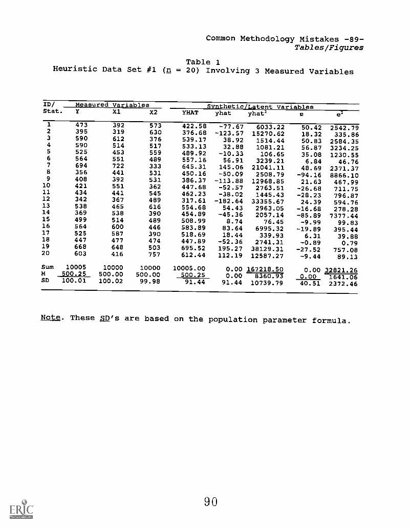
Common Methodology Mistakes -89-Tables/Figures
Table 1Heuristic Data Set #1 (n = 20) Involving 3 Measured Variables
ID/Stat.
Measured Variables Synthetic/Latent VariablesY X1 X2 YHAT yhat yhat2 e e2
1 473 392 573 422.58 -77.67 6033.22 50.42 2542.792 395 319 630 376.68 -123.57 15270.62 18.32 335.863 590 612 376 539.17 38.92 1514.44 50.83 2584.354 590 514 517 533.13 32.88 1081.21 56.87 3234.255 525 453 559 489.92 -10.33 106.65 35.08 1230.556 564 551 489 557.16 56.91 3239.21 6.84 46.767 694 722 333 645.31 145.06 21041.11 48.69 2371.378 356 441 531 450.16 -50.09 2508.79 -94.16 8866.109 408 392 531 386.37 -113.88 12968.85 21.63 467.9910 421 551 362 447.68 -52.57 2763.51 -26.68 711.7511 434 441 545 462.23 -38.02 1445.43 -28.23 796.8712 342 367 489 317.61 -182.64 33355.67 24.39 594.76
13 538 465 616 554.68 54.43 2963.05 -16.68 278.2814 369 538 390 454.89 -45.36 2057.14 -85.89 7377.4415 499 514 489 508.99 8.74 76.45 -9.99 99.8316 564 600 446 583.89 83.64 6995.32 -19.89 395.4417 525 587 390 518.69 18.44 339.93 6.31 39.8818 447 477 474 447.89 -52.36 2741.31 -0.89 0.7919 668 648 503 695.52 195.27 38129.31 -27.52 757.0820 603 416 757 612.44 112.19 12587.27 -9.44 89.13
Sum 10005 10000 10000 10005.00 0.00 167218.50 0.00 32821.26M 500.25 500.00 500.00 500.25 0.00 8360.93 0.00 1641.06SD 100.01 100.02 99.98 91.44 91.44 10739.79 40.51 2372.46
Note. These SD's are based on the population parameter formula.
9 0
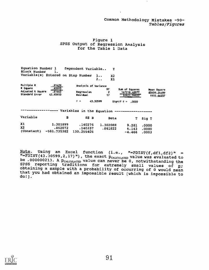
Common Methodology Mistakes -90-Tables/Figures
Figure 1SPSS Output of Regression Analysis
for the Table 1 Data
Equation Number 1 Dependent Variable.Block Number 1.Variable(s) Entered on Step Number 1.. X2
2.. X1
Multiple R .91429 Analysis of VarianceR Square .83593 DF Sum of Squares Mean SquareAdjusted R Square .81662 Regression 2 167218.48977 83609.24489Standard Error 43.93930 Residual 17 321121-:26025- 1930.66237
Variable
43.30599 Signif F = .0000
Variables in the Equation
SE B Beta T Sig T
X1 1.301899 .140276 1.302088 9.281 .0000X2 .862072 .140337 .861822 6.143 .0000(Constant) 581.735382 130.255405 4.466 .0003
Note. Using an Excel function (i.e., "=FDIST(f,dfl,df2)" ="=FDIST(43.30599,2,17)"), the exact pcmzuLATED value was evaluated tobe .000000213. A PCALCUIATED value can never be 0, notwithstanding theSPSS reporting traditions for extremely small values of 2;obtaining a sample with a probability of occurring of 0 would meanthat you had obtained an impossible result [which is impossible todo!].
91

Common Methodology Mistakes -91-Tables/Figures
Figure 2SPSS Output of Bivariate Product-moment Correlation Coefficients
for the 3 Measured and 2 Synthetic Variablesfor Heuristic Data Set #1 (Table 1)
Y X1 X2 E YHATa
Y 1.0000 .6868 -.0677 .4051 .9143( 20) ( 20) ( 20) ( 20) ( 20)P= . P= .001 P= .777 P= .076 P= .000
b cX1 .6868 1.0000 -.7139 .0000 .7512
( 20) ( 20) ( 20) ( 20) ( 20)P= .001 P= . P= .000 P=1.000 P= .000
b cX2 -.0677 -.7139 1.0000 .0000 -.0741
( 20) ( 20) ( 20) ( 20) ( 20)P= .777 P= .000 P= . P=1.000 P= .756
b b bE .4051 .0000 .0000 1.0000 .0000
( 20) ( 20) ( 20) ( 20) ( 20)P= .076 P=1.000 P=1.000 P= . P=1.000
a c c bYHAT .9143 .7512 -.0741 .0000 1.0000
( 20) ( 20) ( 20) ( 20) ( 20)P= .000 P= .000 P= .756 P=1.000 P= .
a A
The bivariate r between the Y and the Y scores is always themultiple R.
AThe measured variables and the synthetic variable Y always have acorrelation of 0 with the synthetic variable e scores.
The structure coefficients for the two measured predictorvariables. This can also be computed as rs= r for a given measuredpredictor with Y / R (Thompson & Borrello, 1985). For example,.6868 / .9143 = .7512.
9 2

Common Methodology Mistakes -92-Tables/Figures
Table 2Heuristic Data Set #2 (n = 20) Involving Scores of 10 People in
Each of Two Groups on 2 Measured Response Variables
Group/ Meas. Vars. LatentStatistic X Y Score
1 1 0 -1.225 aeraa997.wkl 3/8/991 1 0 -1.2251 12 12 0.0001 12 12 0.0001 12 12 0.0001 13 11 -2.4501 13 11 -2.4501 13 11 -2.4501 24 23 -1.2251 24 23 -1.225
2 0 1 1.2252 0 1 1.2252 11 13 2.4502 11 13 2.4502 11 13 2.4502 12 12 0.0002 12 12 0.0002 12 12 0.0002 23 24 1.2252 23 24 1.225
StandardizedDifference 0.137 -0.137 -2.582MI 12.50 11.50 -1.23SDI 7.28 7.28 0.95
M2 11.50 12.50 1.23SD2 7.28 7.28 0.95
12.00 12.00 0.00SD 7.30 7.30 1.55
Note. The tabled SD values are the parameter estimates (i.e., [SOS/ n]'5 = [530.5 / 10]3 = 53.053 = 7.28) . The equivalent valuesassuming a sample estimate of the population a are larger (i.e.,[SOS / (n-1)13 = [530.5 / 9]3 = 58.943 = 7.68).
The latent variable scores were computed by applying the rawdiscriminant function coefficient weights, reported in Figure 3 as-1.225 and 1.225, respectively, to the two measured variables. Forexample, "Latent Scorel" or DSCORE1 equals [(-1.225 x 1) +(1.225 x0)] equals -1.225.
9 3

Common Methodology Mistakes -93-Tables/Figures
Figure 3SPSS Output for 2 ANOVAs and a DDA/MANOVA
for the Table 2 Data
EFFECT .. GROUPMultivariate Tests of Significance (S = 1, M = 0, N = 7 1/2)
Test Name Value Exact F Hypoth. DF Error DF Sig. of F
Pillais .62500 14.16667 2.00 17.00 .000Hotellings 1.66667 14.16667 2.00 17.00 .000Wilks .37500 14.16667 2.00 17.00 .000Roys .62500Note.. F statistics are exact.
Multivariate Effect Size
TEST NAME Effect Size
(All) .625
EFFECT .. GROUP (Cont.)Univariate F-tests with (1,18) D. F.
Variable Hypoth. SS ErrorSSHypoth. MS Error MS F Sig. of FETA Square
X 5.00000 1061.00000 5.00000 58.94444 .08483 .774 .004695.00000 1061.00000 5.00000 58.94444 .08483 .774 .00469
EFFECT .. GROUP (Cont.)Raw discriminant function coefficients
Function No.
Variable 1
-1.2251.225
Note. Using an Excel function (i.e., "=FDIST(f,dfl,df2)" ="=FDIST(14.16667,2,17)"), the exact pcuzuum) value was evaluated tobe .000239. A DCALCULATED value can never be 0, notwithstanding theSPSS reporting traditions for extremely small values of 2;obtaining a sample with a probability of occurring of 0 would meanthat you had obtained an impossible result [which is impossible todo!].

Common Methodology Mistakes -94-Tables/Figures
Figure 4SPSS ANOVA Output for the Multivariate Synthetic Variable
for the DDA/MANOVA Results
Variable DSCOREBy Variable GROUP
Analysis of Variance
Sum of MeanSource D.F. Squares Squares Ratio Prob.
Between Groups 1 30.0125 30.0125 30.0000 .0000Within Groups 18 18.0075 1.0004Total 19 48.0200
Note. The degrees of freedom from this ANOVA of the DDA/MANOVAsynthetic variables (i.e., "DSCORE") are wrong, because thecomputer does not realize that the multivariate synthetic variable,"DSCORE," actually is a composite of two measured variables, and sotherefore the F and p values are also wrong. However, the eta2 canbe computed as 30.0125 / 48.020 = .625 , which exactly matches themultivariate effect size for the DDA/MANOVA reported by SPSS.
95
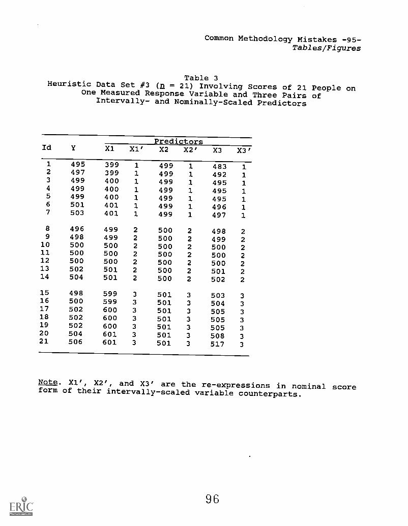
Common Methodology Mistakes -95-Tables/Figures
Table 3Heuristic Data Set #3 (n = 21) Involving Scores of 21 People on
One Measured Response Variable and Three Pairs ofIntervally- and Nominally-Scaled Predictors
PredictorsId Y X1 X1' X2 X2' X3 X3'
1 495 399 1 499 1 483 12 497 399 1 499 1 492 13 499 400 1 499 1 495 14 499 400 1 499 1 495 15 499 400 1 499 1 495 16 501 401 1 499 1 496 17 503 401 1 499 1 497 1
8 496 499 2 500 2 498 29 498 499 2 500 2 499 2
10 500 500 2 500 2 500 211 500 500 2 500 2 500 212 500 500 2 500 2 500 213 502 501 2 500 2 501 214 504 501 2 500 2 502 2
15 498 599 3 501 3 503 316 500 599 3 501 3 504 317 502 600 3 501 3 505 318 502 600 3 501 3 505 319 502 600 3 501 3 505 320 504 601 3 501 3 508 321 506 601 3 501 3 517 3
Note. X1', X2', and X3' are the re-expressions in nominal scoreform of their intervally-scaled variable counterparts.
9 6

Common Methodology Mistakes -96-Tables/Figures
Figure 5Regression (Y, X3) and ANOVA (Y, X3') of Table 3 Data
Regression (Y, X3)
Equation Number 1 Dependent Variable..
Block Number 1. Method: Enter X3
Analysis of VarianceMultiple R .77282 DF Sum of Squares Mean SquareR Square .59725 Regression 1 91.18013 91.18013Adjusted R Square .57605 Residual 19 61.48654 3.23613Standard Error 1.79893
F = 28.17564 Signif F = .0000
ANOVA (Y, X3')
Variable YBy Variable X3A
Analysis of Variance
Sum of Mean F FSource D.F. Squares Squares Ratio Prob.
Between Groups 2 32.6667 16.3333 2.4500 .1145Within Groups 18 120.0000 6.6667Total 20 152.6667
Note. Using an Excel function (i.e., "=FDIST(f,dfl,df2)" ="=FDIST(28.17564,1,19)"), the exact pcLcuu,m) value was evaluated tobe .0000401. For the ANOVA, eta2 was computed to be 21.39% (32.6667/ 152.6667).
97

Common Methodology Mistakes -97-Tables/Figures
Table 4My Most Recent Essays Regarding Statistical Tests
Thompson, B. (1996). AERA editorial policies regarding statisticalsignificance testing: Three suggested reforms. EducationalResearcher, 25(2), 26-30.
Thompson, B. (1997). Editorial policies regarding statisticalsignificance tests: Further comments. Educational Researcher,26(5), 29-32.
Thompson, B. (1998). Statistical significance and effect sizereporting: Portrait of a possible future. Research in theSchools, 5(2), 33-38.
Vacha-Haase, T., & Thompson, B. (1998). Further comments onstatistical significance tests. Measurement and Evaluation inCounseling and Development, 31, 63-67.
Thompson, B. (1998). In praise of brilliance: Where that praisereally belongs. American Psychologist, 53, 799-800.
Thompson, B. (1999). Improving research clarity and usefulness witheffect size indices as supplements to statistical significancetests. Exceptional Children, 65, 329-337.
Thompson, B. (1999). Statistical significance tests, effect sizereporting, and the vain pursuit of pseudo-objectivity. Theory& Psychology, 9(2), 193-199.
Thompson, B. (1999). Why "encouraging" effect size reporting is notworking: The etiology of researcher resistance to changingpractices. Journal of Psychology, 133, 133-140.
Thompson, B. (1999). If statistical significance tests arebroken/misused, what practices should supplement or replacethem?. Theory & Psychology, 9(2), 167-183.
Thompson, B. (in press). Journal editorial policies regardingstatistical significance tests: Heat is to fire as p is toimportance. Educational Psychology Review.

Common Methodology Mistakes -98-Tables/Figures
Table 5Heuristic Data Set #3 Defining a Population of N=20 Scores
3/7/99
ID X
12
3
4
5
67
89
1011121314151617181920
430431432433435438442446451457465474484496512530560595649840
aeraa993.wk4aeraa993.out
A 500.00a 97.73
9 9
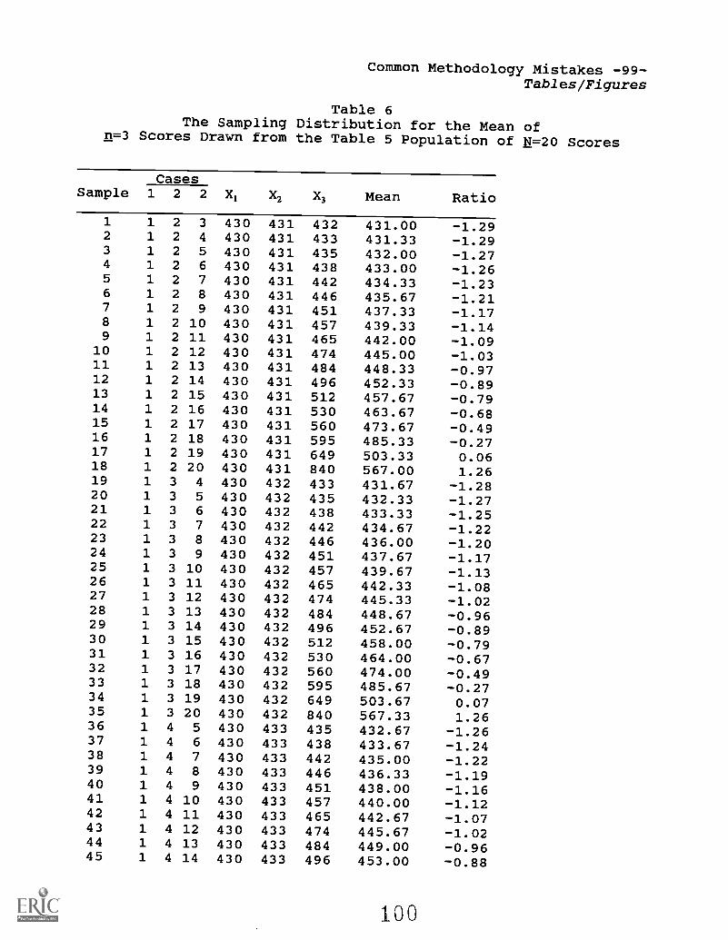
Common Methodology Mistakes -99-Tables/Figures
Table 6The Sampling Distribution for the Mean of
n=3 Scores Drawn from the Table 5 Population of N=20 Scores
SampleCases
X1 X2 X3 Mean Ratio1 2 2
1 1 2 3 430 431 432 431.00 -1.292 1 2 4 430 431 433 431.33 -1.293 1 2 5 430 431 435 432.00 -1.274 1 2 6 430 431 438 433.00 -1.265 1 2 7 430 431 442 434.33 -1.236 1 2 8 430 431 446 435.67 -1.217 1 2 9 430 431 451 437.33 -1.178 1 2 10 430 431 457 439.33 -1.149 1 2 11 430 431 465 442.00 -1.09
10 1 2 12 430 431 474 445.00 -1.0311 1 2 13 430 431 484 448.33 -0.9712 1 2 14 430 431 496 452.33 -0.8913 1 2 15 430 431 512 457.67 -0.7914 1 2 16 430 431 530 463.67 -0.6815 1 2 17 430 431 560 473.67 -0.4916 1 2 18 430 431 595 485.33 -0.2717 1 2 19 430 431 649 503.33 0.0618 1 2 20 430 431 840 567.00 1.2619 1 3 4 430 432 433 431.67 -1.2820 1 3 5 430 432 435 432.33 -1.2721 1 3 6 430 432 438 433.33 -1.2522 1 3 7 430 432 442 434.67 -1.2223 1 3 8 430 432 446 436.00 -1.2024 1 3 9 430 432 451 437.67 -1.1725 1 3 10 430 432 457 439.67 -1.1326 1 3 11 430 432 465 442.33 -1.0827 1 3 12 430 432 474 445.33 -1.0228 1 3 13 430 432 484 448.67 -0.9629 1 3 14 430 432 496 452.67 -0.8930 1 3 15 430 432 512 458.00 -0.7931 1 3 16 430 432 530 464.00 -0.6732 1 3 17 430 432 560 474.00 -0.4933 1 3 18 430 432 595 485.67 -0.2734 1 3 19 430 432 649 503.67 0.0735 1 3 20 430 432 840 567.33 1.2636 1 4 5 430 433 435 432.67 -1.2637 1 4 6 430 433 438 433.67 -1.2438 1 4 7 430 433 442 435.00 -1.2239 1 4 8 430 433 446 436.33 -1.1940 1 4 9 430 433 451 438.00 -1.1641 1 4 10 430 433 457 440.00 -1.1242 1 4 11 430 433 465 442.67 -1.0743 1 4 12 430 433 474 445.67 -1.0244 1 4 13 430 433 484 449.00 -0.9645 1 4 14 430 433 496 453.00 -0.88

Common Methodology Mistakes -100-Tables/Figures
46 1 4 15 430 433 512 458.33 -0.7847 1 4 16 430 433 530 464.33 -0.6748 1 4 17 430 433 560 474.33 -0.4849 1 4 18 430 433 595 486.00 -0.2650 1 4 19 430 433 649 504.00 0.0751 1 4 20 430 433 840 567.67 1.2752 1 5 6 430 435 438 434.33 -1.2353 1 5 7 430 435 442 435.67 -1.2154 1 5 8 430 435 446 437.00 -1.1855 1 5 9 430 435 451 438.67 -1.1556 1 5 10 430 435 457 440.67 -1.1157 1 5 11 430 435 465 443.33 -1.0658 1 5 12 430 435 474 446.33 -1.0159 1 5 13 430 435 484 449.67 -0.9460 1 5 14 430 435 496 453.67 -0.8761 1 5 15 430 435 512 459.00 -0.7762 1 5 16 430 435 530 465.00 -0.6663 1 5 17 430 435 560 475.00 -0.4764 1 5 18 430 435 595 486.67 -0.2565 1 5 19 430 435 649 504.67 0.0966 1 5 20 430 435 840 568.33 1.2867 1 6 7 430 438 442 436.67 -1.1968 1 6 8 430 438 446 438.00 -1.1669 1 6 9 430 438 451 439.67 -1.1370 1 6 10 430 438 457 441.67 -1.0971 1 6 11 430 438 465 444.33 -1.0472 1 6 12 430 438 474 447.33 -0.9973 1 6 13 430 438 484 450.67 -0.9274 1 6 14 430 438 496 454.67 -0.8575 1 6 15 430 438 512 460.00 -0.7576 1 6 16 430 438 530 466.00 -0.6477 1 6 17 430 438 560 476.00 -0.4578 1 6 18 430 438 595 487.67 -0.2379 1 6 19 430 438 649 505.67 0.1180 1 6 20 430 438 840 569.33 1.3081 1 7 8 430 442 446 439.33 -1.1482 1 7 9 430 442 451 441.00 -1.1183 1 7 10 430 442 457 443.00 -1.0784 1 7 11 430 442 465 445.67 -1.0285 1 7 12 430 442 474 448.67 -0.96
1131 16 17 18 530 560 595 561.67 1.161132 16 17 19 530 560 649 579.67 1.491133 16 17 20 530 560 840 643.33 2.691134 16 18 19 530 595 649 591.33 1.711135 16 18 20 530 595 840 655.00 2.901136 16 19 20 530 649 840 673.00 3.241137 17 18 19 560 595 649 601.33 1.901138 17 18 20 560 595 840 665.00 3.091139 17 19 20 560 649 840 683.00 3.431140 18 19 20 595 649 840 694.67 3.65
101

Common Methodology Mistakes -101-Tables/Figures
Figure 6Graphic Presentation of the Sampling Distribution for the Mean of
n=3 Scores Drawn from the Table 5 Population of N=20 Scores
Count Midpoint60 433 1************:**
146 446 1****************:********************160 459 1********************:*******************135 472 1***********************:**********123 465 1**************************:****96 496 1************************97 511 1************************67 524 1*****************38 537 1**********21 550 I*****28 563 I*******50 576 I*********:***35 589 I******:**24 602 I***:**17 615 I**:*17 628 I*:**14 641 I:***6 654 I**4 667 I*1 680 I
1 693 I
0 40 80 120 160 200Histogram frequency
MEANMean 500.000 Std err 1.581 Median 486.000Mode 457.670 Std dev 53.395 Variance 2850.986Kurtosis .418 S E Kurt .145 Skewness 1.052S E Skew .072 Range 263.670 Minimum 431.000Maximum 694.670 Sum 570000.020
Percentile Value Percentile Value Percentile Value1.00 433.330 2.00 435.000 3.00 436.6704.00 437.881 5.00 439.016 6.00 440.0007.00 441.330 8.00 442.425 9.00 443.330
10.00 444.670 11.00 445.670 12.00 446.33025.00 459.000 50.00 486.000 75.00 524.50288.00 577.723 89.00 581.000 90.00 584.96791.00 588.670 92.00 592.908 93.00 597.71394.00 602.210 95.00 610.313 96.00 617.36097.00 625.440 98.00 639.729 99.00 648.865
102

Common Methodology Mistakes -102-Tables/Figures
Figure 7Graphic Presentation of the Test Distribution for the Mean ofn=3 Scores Drawn from the Table 5 Population of N=20 Scores
Count Midpoint39 -1.30 I********** .
143 -1.05 1***************:********************159 -.80 1********************:*******************147 -.55 1***********************:*************125 -.30 1**************************:****105 -.05 I**************************99 .20 1*************************68 .45 I*****************37 .70 1*********21 .95 I*****33 1.20 I********49 1.45 1*********:**35 1.70 I******:**25 1.95 I***:**19 2.20 I**:**12 2.45 I:**14 2.70 I:***5 2.95 I*3 3.20 I*1 3.45 I1 3.70 I
0 40 80 120Histogram frequency
160 200
TRATIOMean .000 Std err .030 Median -.262Mode -.793 Std dev 1.000 Variance 1.001Kurtosis .418 S E Kurt .145 Skewness 1.052S E Skew .072 Range 4.940 Minimum -1.293Maximum 3.647 Sum .000
Percentile Value Percentile Value Percentile Value
1.00 -1.249 2.00 -1.218 3.00 -1.1874.00 -1.164 5.00 -1.143 6.00 -1.1247.00 -1.099 8.00 -1.079 9.00 -1.06210.00 -1.037 11.00 -1.018 12.00 -1.00625.00 -.768 50.00 -.262 75.00 .45988.00 1.456 89.00 1.518 90.00 1.59291.00 1.661 92.00 1.741 93.00 1.83194.00 1.915 95.00 2.067 96.00 2.19997.00 2.350 98.00 2.618 99.00 2.789

Common Methodology Mistakes -103-Tables/Figures
Table 7Two Illustrative "Modern" Statistics
Id X X' X-
12
3
430431432
433433433
----
4 433 433 4335 435 435 4356 438 438 4387 442 442 4428 446 446 4469 451 451 451
10 457 457 45711 465 465 46512 474 474 47413 484 484 48414 496 496 49615 512 512 51216 530 530 53017 560 560 56018 595 560 0119 649 56020 840 560
500.00 480.10 473.07Md 461.00 461.00 461.00SD 100.27 49.34 38.98
2.40 0.72 1.046.54 -1.08 0.30
aera992.wkl 3/6/99
104

Common Methodology Mistakes -104-Tables/Figures
Table 8Heuristic Data Set #4 for use in Illustrating
the Univariate Bootstrap
3/7/99
IDVariables
Churches Murders Population
1
2
3
4
5
6
7
8
9
101112131415161718192021222324252627282930313233343536373839404142
35052023286314752011170913131098937836997582645663
1010875615912559899329
11621372355867
11292441527909
1328921982829
1328133912831439999
1052142813451423
198410569215864474203733262111661511411381341321251138988785249444237272424232219171413121212119
7
6
6
7322564348555727837261027974162990215855771007618736014935393641432589305
1110623579396983403741952672971723959575396573058571059567306576396643955782224529401574932525439600499569396592669527432602993524953574039567496505955572039523085568206524099526199580284
aera994.wkl
105

Common Methodology Mistakes -105-Tables/Figures
43 662 3 52294344 1295 2 53029945 1225 0 521944
Note. The first 15 cases are actual data reported by Waliczek(1996).

Common Methodology Mistakes -106-Tables/Figures
Figure 8Scatterplot of the Table 8 Heuristic Data
PLOT OF MURDERS WITH CHURCHES
2000+
1750+
1500+
1250+
1E 1000+
750+
1
500+1
11
250+1
12 1111
I 2 2 10+1 1 12 21 I 12412 1
250 750 1250 1750 2250 2750 3250 3750CHURCHES
Note. r2 = 60.8%; a = -362.363; b = .468.
107
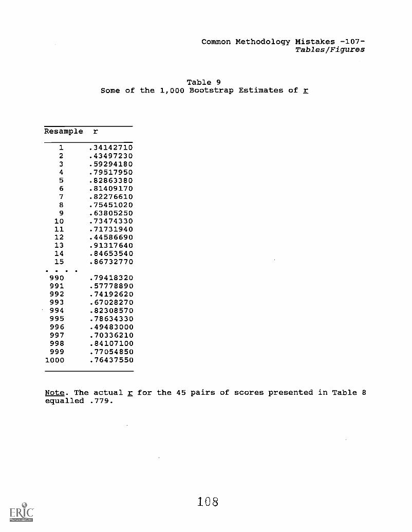
Common Methodology Mistakes -107-Tables/Figures
Table 9Some of the 1,000 Bootstrap Estimates of r
Resample r
1 .341427102 .434972303 .592941804 .795179505 .828633806 .814091707 .822766108 .754510209 .63805250
10 .7347433011 .7173194012 .4458669013 .9131764014 .8465354015 .86732770.
990 .79418320991 .57778890992 .74192620993 .67028270994 .82308570995 .78634330996 .49483000997 .70336210998 .84107100999 .770548501000 .76437550
Note. The actual r for the 45 pairs of scores presented in Table 8equalled .779.
108
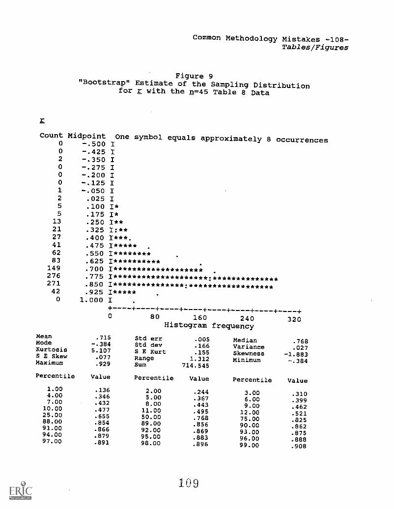
Common Methodology Mistakes -108-Tables/Figures
Figure 9"Bootstrap" Estimate of the Sampling Distribution
for r with the n=45 Table 8 Data
Count Midpoint One symbol equals approximately 8 occurrences0 -.500 I0 -.425 I2 -.350 I0 -.275 I0 -.200 I0 -.125 I1 -.050 I2 .025 I5 .100 I*5 .175 I*
13 .250 I**21 .325 I:**27 .400 I***.41 .475 I*****62 .550 I********83 .625 I**********
149 .700 I*******************276 .775 I********************:**************271 .850 I***************:******************42 .925 I*****0 1.000 I
0 80 160 240Histogram frequency
320
Mean .715 Std err .005 Median .768Mode -.384 Std dev .166 Variance .027Kurtosis 5.107 S E Kurt .155 Skewness -1.883S E Skew .077 Range 1.312 Minimum -.384Maximum .929 Sum 714.545
Percentile Value Percentile Value Percentile Value1.00 .136 2.00 .244 3.00 .3104.00 .346 5.00 .367 6.00 .3997.00 .432 8.00 .443 9.00 .46210.00 .477 11.00 .495 12.00 .52125.00 .655 50.00 .768 75.00 .82588.00 .854 89.00 .856 90.00 .86291.00 .866 92.00 .869 93.00 .87594.00 .879 95.00 .883 96.00 .88897.00 .891 98.00 .896 99.00 .908
109
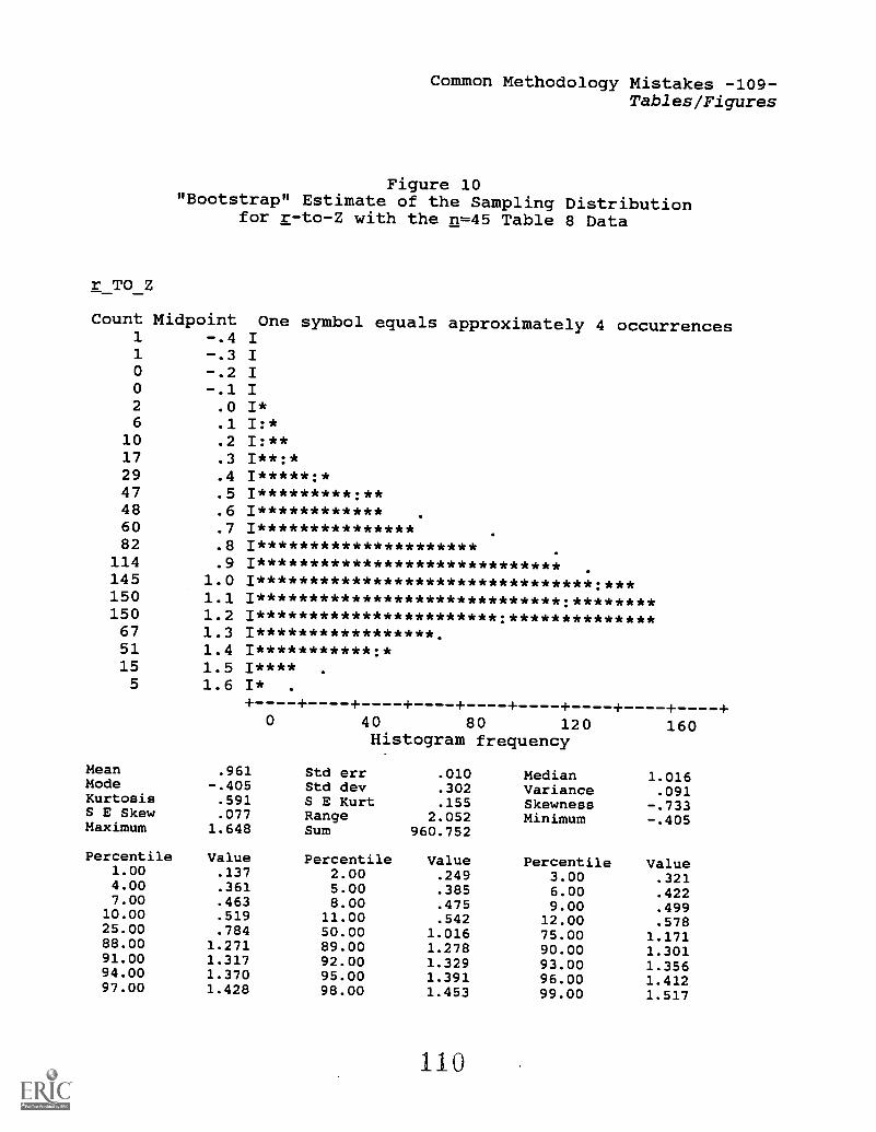
Common Methodology Mistakes -109-Tables/Figures
Figure 10"Bootstrap" Estimate of the Sampling Distribution
for r-to-Z with the n=45 Table 8 Data
r_TO_Z
Count Midpoint One symbol equals approximately 4 occurrences1 -.4 I1 -.3 I0 -.2 I0 -.1 I2 .0 I*6 .1 I:*
10 .2 I:**17 .3 I**:*29 .447 .5 1*********:**48 .6 1************60 .7 1***************82 .8 1*********************
114 .8 1*****************************145 1.0 I********************************:***150 1.1 I*****************************:********150 1.2 1***********************:**************67 1.3 1*****************.51 1.4 1***********:*15 1.5 I**** .
5 1.6 I* .
0 40 80 120Histogram frequency
160
Mean .961 Std err .010 Median 1.016Mode -.405 Std dev .302 Variance .091Kurtosis .591 S E Kurt .155 Skewness -.733S E Skew .077 Range 2.052 Minimum -.405Maximum 1.648 Sum 960.752
Percentile Value Percentile Value Percentile Value1.00 .137 2.00 .249 3.00 .3214.00 .361 5.00 .385 6.00 .4227.00 .463 8.00 .475 9.00 .49910.00 .519 11.00 .542 12.00 .57825.00 .784 50.00 1.016 75.00 1.17188.00 1.271 89.00 1.278 90.00 1.30191.00 1.317 92.00 1.329 93.00 1.35694.00 1.370 95.00 1.391 96.00 1.41297.00 1.428 98.00 1.453 99.00 1.517
110

Common Methodology Mistakes -110-Tables/Figures
Table 10Percentiles of Resampled Sampling Distributions for
r-to-Z Values for the Table 8 Data with100 and 1,000 Resamples
aeraa996.wkl 3/8/99
%ile/ n of ResamplesStatistic 100 1000 Difference
99 1.453 1.517 -0.06498 1.424 1.453 -0.02997 1.405 1.428 -0.02396 1.393 1.412 -0.01995 1.352 1.391 -0.03994 1.341 1.370 -0.02993 1.309 1.356 -0.04792 1.298 1.329 -0.03191 1.294 1.317 -0.02390 1.289 1.301 -0.01289 1.284 1.278 0.00688 1.279 1.271 0.008
75 1.195 1.171 0.024
Mean 1.000 0.961 0.039(SD) (0.267) (0.302)
50 1.063 1.016 0.047
25 0.783 0.784 -0.001
12 0.657 0.578 0.07911 0.654 0.542 0.11210 0.634 0.519 0.1159 0.567 0.499 0.0688 0.553 0.475 0.0787 0.543 0.463 0.0806 0.494 0.422 0.0725 0.476 0.385 0.0914 0.416 0.361 0.0553 0.362 0.321 0.0412 0.337 0.249 0.0881 0.303 0.137 0.166
111

Common Methodology Mistakes -111-Tables/Figures
Figure 11DDA/MANOVA Results for Sir Ronald Fisher's (1936) Iris Data
(k groups = 3; n = 150; p response variables = 4)
DISCRIMINANT FUNCTION CENTROIDS
GroupFunction
I II
1 -5.50285 6.876732 3.93011 5.933673 7.88771 7.17438
DISCRIMINANT FUNCTION COEFFICIENTS
Response Function I Coefs Function II CoefsVariables Function rs Function rs
X1 -0.82940 0.11458 0.02410 0.16000X2 -1.53458 -0.04043 2.16458 0.29337X3 2.20126 0.30383 -0.93196 0.07217X4 2.81058 0.12958 2.83931 0.15087
112
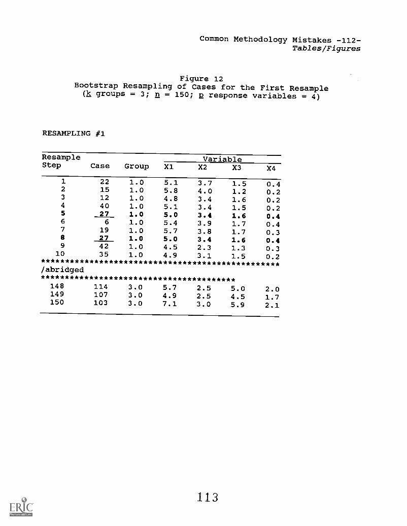
Common Methodology Mistakes -112-Tables/Figures
Figure 12Bootstrap Resampling of Cases for the First Resample(k groups = 3; n = 150; p response variables = 4)
RESAMPLING #1
Resample VariableStep Case Group X1 X2 X3 X4
1 22 1.0 5.1 3.7 1.5 0.42 15 1.0 5.8 4.0 1.2 0.23 12 1.0 4.8 3.4 1.6 0.24 40 1.0 5.1 3.4 1.5 0.25 27 1.0 5.0 3.4 1.6 0.46 6 1.0 5.4 3.9 1.7 0.47 19 1.0 5.7 3.8 1.7 0.38 27 1.0 5.0 3.4 1.6 0.49 42 1.0 4.5 2.3 1.3 0.3
10 35 1.0 4.9 3.1 1.5 0.2*************************************************/abridged****************************************
148 114 3.0 5.7 2.5 5.0 2.0149 107 3.0 4.9 2.5 4.5 1.7150 103 3.0 7.1 3.0 5.9 2.1
113

Common Methodology Mistakes -113-Tables/Figures
Figure 13Resampling Estimates of Statistics for Resamples #1 and #2000
(k groups = 3; n = 150; response variables = 4)
Resample #1
FUNCTION MATRIX BEFORE ROTATION1 -1.53727 0.401132 -0.86791 1.882723 3.02954 -0.963304 1.89711 2.60662
FUNCTION MATRIX AFTER ROTATION1 -1.51555 0.476662 -0.77374 1.923343 2.97819 -1.111944 2.02369 2.50962
STRUCTURE MATRIX BASED ON ROTATED FUNCTION1 0.12341 0.247902 -0.02461 0.347913 0.30382 0.122174 0.13003 0.13888
Resample #2000
FUNCTION MATRIX BEFORE ROTATION1 -1.04205 -0.146412 -1.22630 1.761733 2.47935 -1.280004 2.63734 3.88797
FUNCTION MATRIX AFTER ROTATION1 -1.05126 -0.046472 -1.05290 1.870543 2.34614 -1.510384 2.99575 3.61905
STRUCTURE MATRIX BASED ON ROTATED FUNCTION1 0.10285 0.079362 -0.02377 0.276283 0.28983 -0.007994 0.13456 0.13121
114
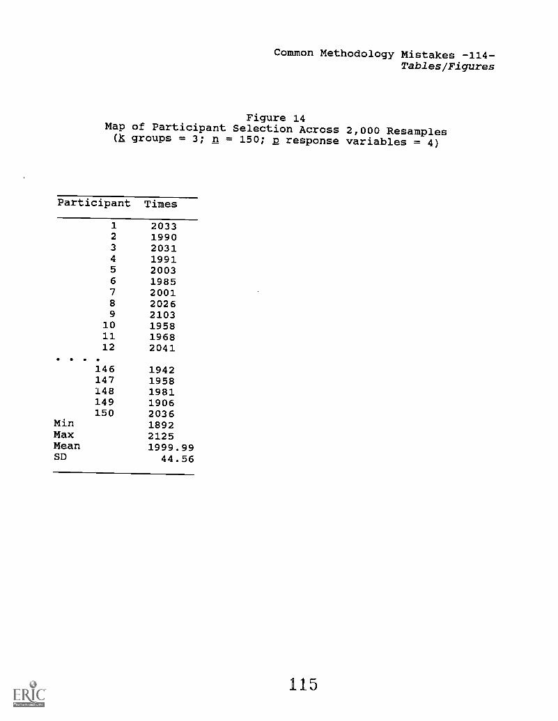
Common Methodology Mistakes -114-Tables/Figures
Figure 14Map of Participant Selection Across 2,000 Resamples(h groups = 3; n = 150; p response variables = 4)
Participant Times
1 20332 19903 20314 19915 20036 19857 20018 20269 2103
10 195811 196812 2041
146 1942147 1958148 1981149 1906150 2036
Min 1892Max 2125Mean 1999.99SD 44.56

Common Methodology Mistakes -115-Tables/Figures
Figure 15Mean (and SD) of Bootstrap Estimates Across 2,000 Resamples
(k groups = 3; n = 150; p response variables = 4)
*** SUMMARY STATISTICS FOR GROUP CENTROIDS:
Group StatisticFunction
1 -5.65456 6.79552SD 1.16636 1.86960
1.63016 -0.2663917.38350 -0.05702
2 4.01345 5.81133SD 1.13114 1.87885
-1.00750 -0.257979.06839 -0.05715
3 8.06143 7.10633SD 1.38417 1.86440
-3.82083 -0.2653649.27710 -0.05739
Var StatisticFunction I Function II
Function rs Function rs
X1 -0.84924 0.10844 0.00669 0.15045SD 0.29921 0.01392 0.61489 0.08020
X2 -1.60807 -0.04132 2.15484 0.278680.39638 0.02294 0.46866 0.02998
X3
SD
2.24008 0.29401 -0.93826 0.06939SD 0.29062 0.01910 0.66124 0.06334
X4 2.91339 0.12619 2.86778 0.14410SD 0.40405 0.01246 0.71420 0.01408
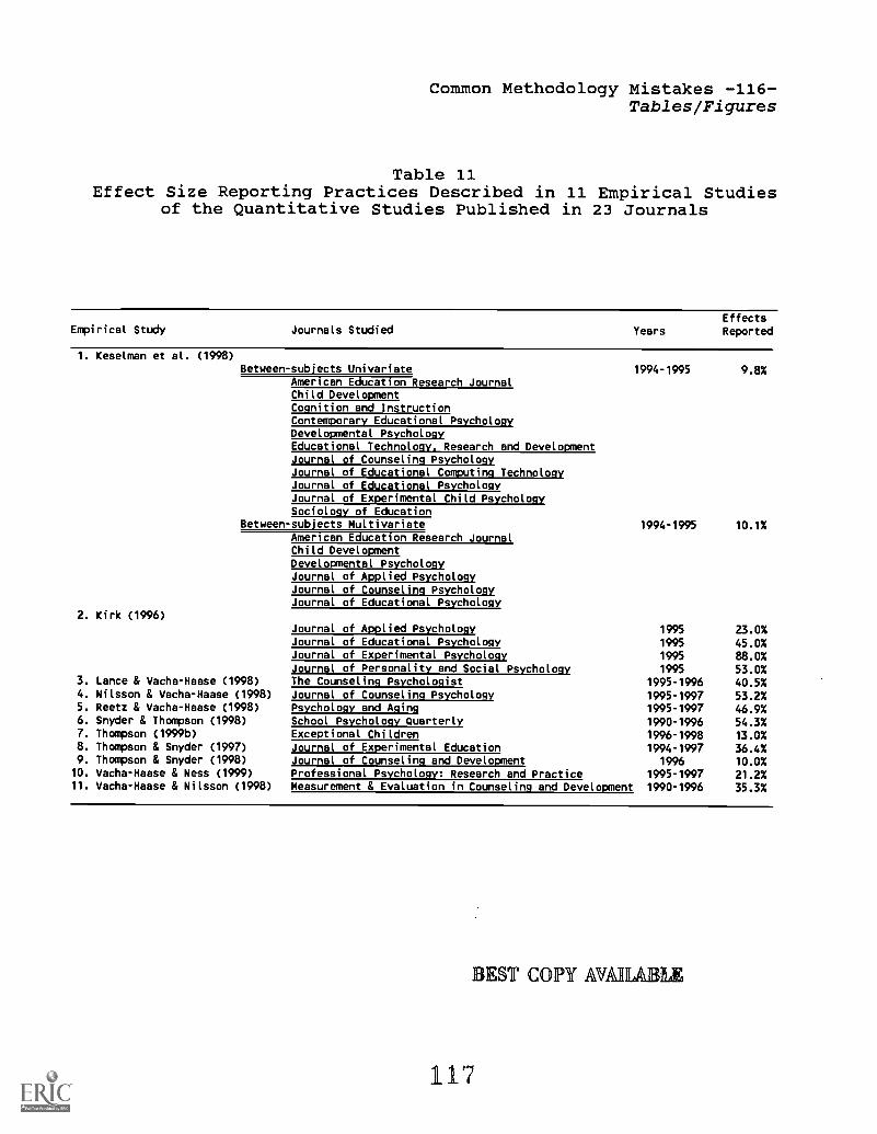
Common Methodology Mistakes -116-Tables/Figures
Table 11Effect Size Reporting Practices Described in 11 Empirical Studies
of the Quantitative Studies Published in 23 Journals
Empirical Study Journals Studied
1. Keselman et al. (1998)Between-subjects Univariate
American Education Research JournalChild DevelopmentCognition and InstructionContemporary Educational PsychologyDevelopmental PsychologyEducational Technology. Research and DevelopmentJournal of Counseling PsychologyJournal of Educational Computing TechnologyJournal of Educational PsychologyJournal of Experimental Child PsychologySociology of Education
Between-subjects MultivariateAmerican Education Research JournalChild DevelopmentDevelopmental PsychologyJournal of Applied PsychologyJournal of Counseling PsychologyJournal of Educational Psychology
2. Kirk (1996)
3. Lance & Vacha-Haase (1998)4. Nilsson & Vacha-Haase (1998)5. Reetz & Vacha-Haase (1998)6. Snyder & Thompson (1998)7. Thompson (1999b)
8. Thompson & Snyder (1997)9. Thompson & Snyder (1998)10. Vacha-Haase & Ness (1999)11. Vacha-Haase & Nilsson (1998)
Journal of Applied PsychologyJournal of Educational PsychologyJournal of Experimental PsychologyJournal of Personality and Social PsychologyThe Counseling PsychologistJournal of Counseling PsychologyPsychology and AgingSchool Psychology QuarterlyExceptional ChildrenJournal of Experimental EducationJournal of Counseling and DevelopmentProfessional Psychology: Research and PracticeMeasurement & Evaluation in Counseling and Development
YearsEffectsReported
1994-1995 9.8%
1994-1995 10.1%
1995 23.0%1995 45.0%1995 asm1995 53.0%
1995-1996 40.5%1995-1997 53.2%1995-1997 46.9%1990-1996 54.3%1996-1998 13.0%1994-1997 36.4%
1996 10.0%1995-1997 21.2%1990-1996 35.3%
BEST COPY AVARLABLE
117
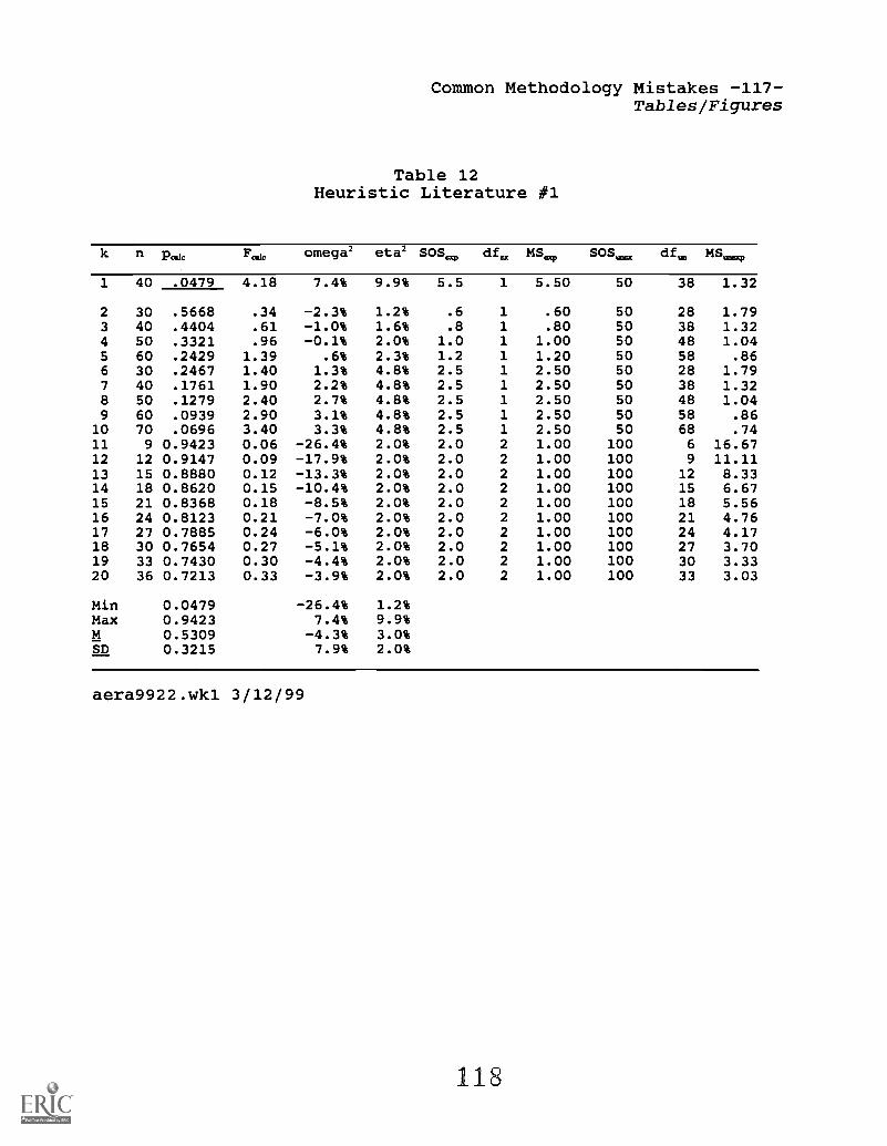
Common Methodology Mistakes -117-Tables/Figures
Table 12Heuristic Literature #1
k n pok F.k omega2 eta2 SOS., df. MS., SOS df. MS
1 40 .0479 4.18 7.4% 9.9% 5.5 1 5.50 50 38 1.32
2 30 .5668 .34 -2.3% 1.2% .6 1 .60 50 28 1.793 40 .4404 .61 -1.0% 1.6% .8 1 .80 50 38 1.324 50 .3321 .96 -0.1% 2.0% 1.0 1 1.00 50 48 1.045 60 .2429 1.39 .6% 2.3% 1.2 1 1.20 50 58 .866 30 .2467 1.40 1.3% 4.8% 2.5 1 2.50 50 28 1.797 40 .1761 1.90 2.2% 4.8% 2.5 1 2.50 50 38 1.328 50 .1279 2.40 2.7% 4.8% 2.5 1 2.50 50 48 1.049 60 .0939 2.90 3.1% 4.8% 2.5 1 2.50 50 58 .86
10 70 .0696 3.40 3.3% 4.8% 2.5 1 2.50 50 68 .7411 9 0.9423 0.06 -26.4% 2.0% 2.0 2 1.00 100 6 16.6712 12 0.9147 0.09 -17.9% 2.0% 2.0 2 1.00 100 9 11.1113 15 0.8880 0.12 -13.3% 2.0% 2.0 2 1.00 100 12 8.3314 18 0.8620 0.15 -10.4% 2.0% 2.0 2 1.00 100 15 6.6715 21 0.8368 0.18 -8.5% 2.0% 2.0 2 1.00 100 18 5.5616 24 0.8123 0.21 -7.0% 2.0% 2.0 2 1.00 100 21 4.7617 27 0.7885 0.24 -6.0% 2.0% 2.0 2 1.00 100 24 4.1718 30 0.7654 0.27 -5.1% 2.0% 2.0 2 1.00 100 27 3.7019 33 0.7430 0.30 -4.4% 2.0% 2.0 2 1.00 100 30 3.3320 36 0.7213 0.33 -3.9% 2.0% 2.0 2 1.00 100 33 3.03
Min 0.0479 -26.4% 1.2%Max 0.9423 7.4% 9.9%M 0.5309 -4.3% 3.0%SD 0.3215 7.9% 2.0%
aera9922.wkl 3/12/99
118
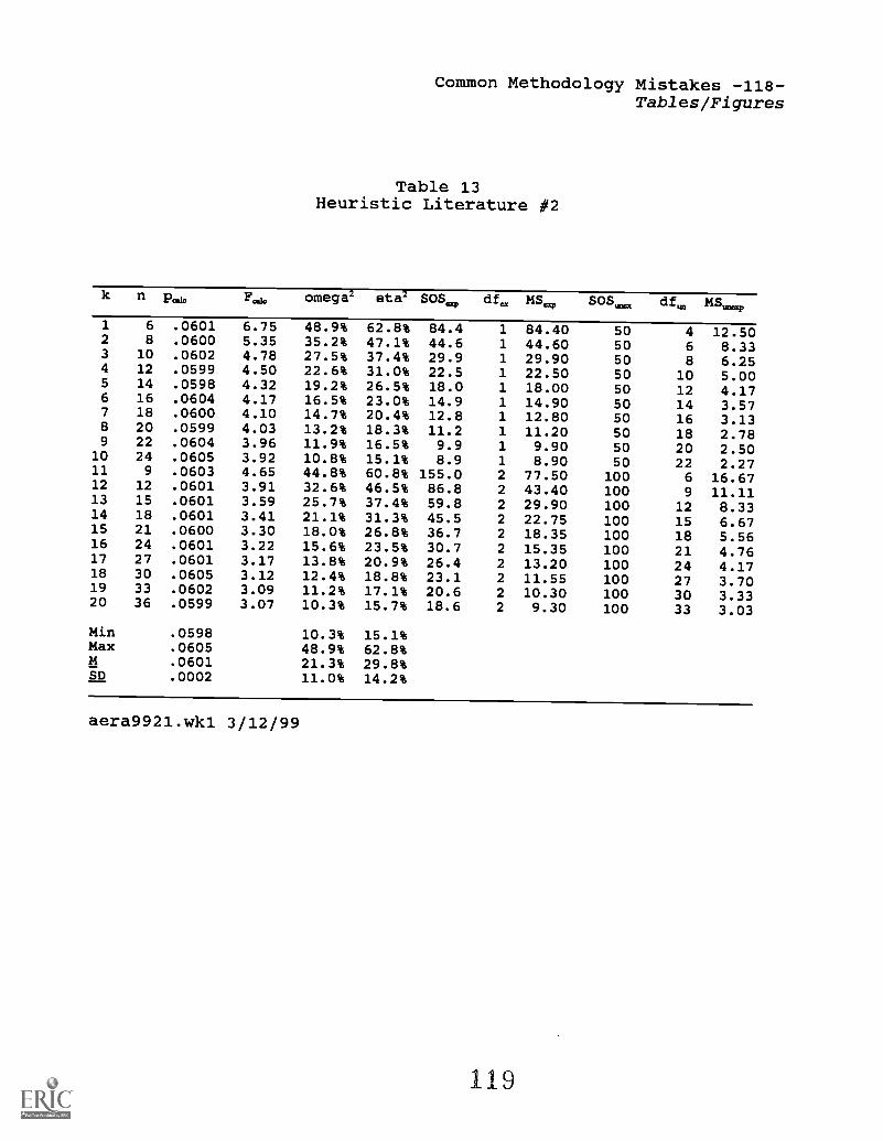
Common Methodology Mistakes -118-Tables/Figures
Table 13Heuristic Literature #2
n pcsk Fad, omega2 eta2 SOS.q, df. MSeip SOS df. MS
1 6 .0601 6.75 48.9% 62.8% 84.4 1 84.40 50 4 12.502 8 .0600 5.35 35.2% 47.1% 44.6 1 44.60 50 6 8.333 10 .0602 4.78 27.5% 37.4% 29.9 1 29.90 50 8 6.254 12 .0599 4.50 22.6% 31.0% 22.5 1 22.50 50 10 5.005 14 .0598 4.32 19.2% 26.5% 18.0 1 18.00 50 12 4.176 16 .0604 4.17 16.5% 23.0% 14.9 1 14.90 50 14 3.577 18 .0600 4.10 14.7% 20.4% 12.8 1 12.80 50 16 3.138 20 .0599 4.03 13.2% 18.3% 11.2 1 11.20 50 18 2.789 22 .0604 3.96 11.9% 16.5% 9.9 1 9.90 50 20 2.5010 24 .0605 3.92 10.8% 15.1% 8.9 1 8.90 50 22 2.2711 9 .0603 4.65 44.8% 60.8% 155.0 2 77.50 100 6 16.67
12 12 .0601 3.91 32.6% 46.5% 86.8 2 43.40 100 9 11.1113 15 .0601 3.59 25.7% 37.4% 59.8 2 29.90 100 12 8.3314 18 .0601 3.41 21.1% 31.3% 45.5 2 22.75 100 15 6.6715 21 .0600 3.30 18.0% 26.8% 36.7 2 18.35 100 18 5.5616 24 .0601 3.22 15.6% 23.5% 30.7 2 15.35 100 21 4.7617 27 .0601 3.17 13.8% 20.9% 26.4 2 13.20 100 24 4.1718 30 .0605 3.12 12.4% 18.8% 23.1 2 11.55 100 27 3.7019 33 .0602 3.09 11.2% 17.1% 20.6 2 10.30 100 30 3.3320 36 .0599 3.07 10.3% 15.7% 18.6 2 9.30 100 33 3.03
Min .0598 10.3% 15.1%Max .0605 48.9% 62.8%M .0601 21.3% 29.8%SD .0002 11.0% 14.2%
aera9921.wkl 3/12/99
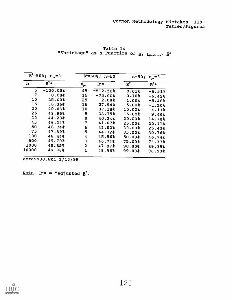
Common Methodology Mistakes -119-Tables/Figures
Table 14"Shrinkage" as a Function of n, nvaham,
R2=50%; niw=3 R2=50%; n=50 n=50; nr,=3
R2* npv R2* R2 R2*5 -100.00% 45 -512.50% 0.01% -6.51%7 0.00% 35 -75.00% 0.10% -6.42%
10 25.00% 25 -2.08% 1.00% -5.46%15 36.36% 15 27.94% 5.00% -1.20%20 40.63% 10 37.18% 10.00% 4.13%25 42.86% 9 38.75% 15.00% 9.46%30 44.23% 8 40.24% 20.00% 14.78%45 46.34% 7 41.67% 25.00% 20.11%50 46.74% 6 43.02% 30.00% 25.43%75 47.89% 5 44.32% 35.00% 30.76%
100 48.44% 4 45.56% 50.00% 46.74%500 49.70% 3 46.74% 75.00% 73.37%
1000 49.85% 2 47.87% 90.00% 89.35%10000 49.98% 1 48.96% 99.00% 98.93%
aera9930.wkl 3/13/99
Note. R2* = "adjusted R2.
120

Common Methodology Mistakes -120-Tables/Figures
Table 15"Shrinkage" as an Interaction Effect
CombinationR2* ShrinkageR2
56 3 13.8% 8.8% 5.0%93 5 13.8% 8.8% 5.0%
128 7 13.8% 8.8% 5.0%166 9 13.8% 8.8% 5.0%200 11 13.8% 8.8% 5.0%19 1 13.8% 8.7% 5.1%38 2 13.8% 8.9% 4.9%56 3 13.8% 8.8% 5.0%74 4 13.8% 8.8% 5.0%93 5 13.8% 8.8% 5.0%50 4 44.0% 39.0% 5.0%40 6 72.5% 67.5% 5.0%30 8 87.0% 82.0% 5.0%
aera9931.wkl 3/13/99
Note. R2* = "adjusted E2. The 13.8% effect size is the value thatCohen (1988, pp. 22-27) characterized as "large," at least asregards result typicality.
121

Table 16
Selected Features of "Classical" and "Modern" Inquiry
"classical" Research Model
Problem
"Modern" Research Model
Introduction
Prior literature is characterized
only as regards whether or not
previous results were statistically
significant.
Hypothesis Formulation
Researchers employ a mindless
"point and click" specification of
"nil" null hypotheses.
Discussion
Results are only evaluated for
statistical significance.
Because p values are confounded
indices jointly influenced by n's
and effect sizes and other factors,
conclusions based on "vote counts"
integrate apples-and-oranges
comparisons.
Hypotheses are not formulated
based on a reflective integration
of theory and specific previous
results.
Studies with large sample sizes and
small effects are overinterpreted;
studies with small sample sizes and
large effects are underinterpreted
(cf. Wampold, Furlong & Atkinson,
1983).
Characterizations of previous
literature include summaries of
prior effect sizes (potentially
including "corrected" effect indices
that adjust for estimated sampling
error).
Null hypotheses are grounded in
specific results from previous
studies.
Effect sizes are always reported and
interpreted in relation to (a) the
valuing of the outcome variable(s) and
(b) the effects reported in the prior
related literature.
CO
PY
AV
AIL
AB
LE
122
Common Methodology Mistakes -121-
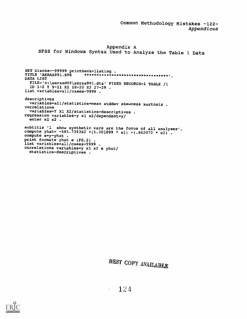
Common Methodology Mistakes -122-Appendices
Appendix ASPSS for Windows Syntax Used to Analyze the Table 1 Data
SET blanks=-99999 printback=listing .
TITLE 'AERAA991.SPSDATA LISTFILE='c:\aeraad99\aeraa991.dta' FIXED RECORDS=1 TABLE /1ID 1-2 Y 9-11 X1 18-20 X2 27-29 .
list variables=all/cases=9999 .
descriptivesvariables=all/statistics=mean stddev skewness kurtosis .
correlationsvariables=Y X1 X2/statistics=descriptives .
regression variables=y xl x2/dependent=y/enter xl x2 .
subtitle '1 show synthetic vars are the focus of all analyses'.compute yhat= -581.735382 +(1.301899 * xl) +(.862072 * x2) .
compute e=y-yhat .
print formats yhat e (F8.2) .
list variables=all/cases=9999 .
correlations variables=y xl x2 e yhat/statistics=descriptives .
BEST COPY AVAILABLE
124
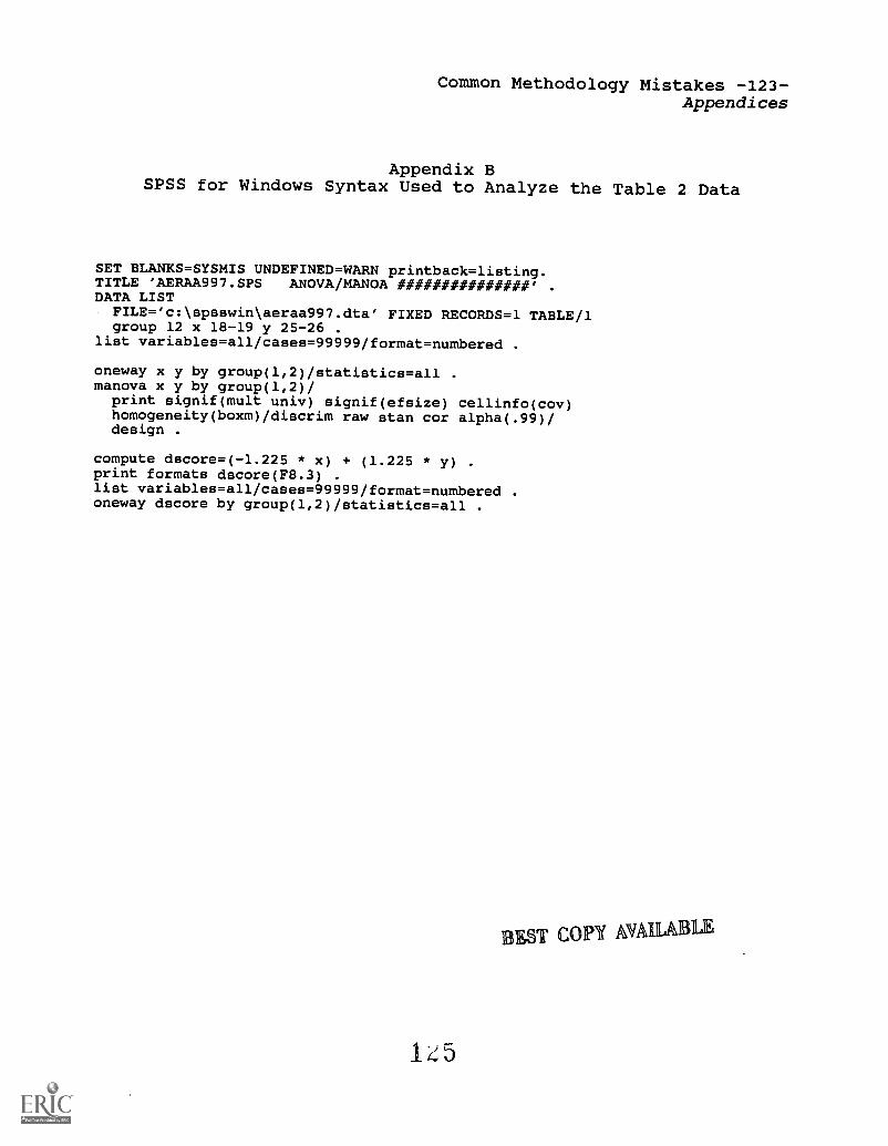
Common Methodology Mistakes -123-Appendices
Appendix BSPSS for Windows Syntax Used to Analyze the Table 2 Data
SET BLANKS=SYSMIS UNDEFINED=WARN printback=listing.TITLE 'AERAA997.SPS ANOVA/MANOA ###############' .
DATA LISTFILE='c:\apsewin\aeraa997.dta' FIXED RECORDS=1 TABLE/1group 12 x 18-19 y 25-26 .
list variables=all/cases=99999/format=numbered .
oneway x y by group(1,2)/statistics=all .
manova x y by group(1,2)/print signif(mult univ) signif(efsize) cellinfo(cov)homogeneity(boxm)/discrim raw stan cor alpha(.99)/design .
compute dscore=(-1.225 * x) + (1.225 * y) .
print formats dscore(F8.3) .
list variables=all/caees=99999/format=numbered .
oneway dscore by group(1,2)/statistics=all .
BEST COPY AVAIUBLE

Common Methodology Mistakes -124-Appendices
Appendix CSPSS for Windows Syntax Used to Analyze the Table 3 Data
SET BLANKS=SYSMIS UNDEFINED=WARN printback=listing.TITLE 'AERA9910.SPS Var Discard ###################'DATA LISTFILE='a:aera9910.dta' FIXED RECORDS=1 TABLE/1id 1-2 y 7-9 x3 14-16 x3a 20 .
list variables=all/cases=99999/format=numbered .
descriptives variables=all/statistics=all .
regression variables=y x3/dependent=y/enter x3 .
oneway y by x3a(1,3)/statistics=all.
EST COPY AVAILABLE

AEA4E- Nv TE b
U.S. DEPARTMENT OF EDUCATIONMace of Educational Research and Improvement 10ER11
Educational Resources information Center (ERIC)
REPRODUCTION RELEASE(Specif ic Document)
I. DOCUMENT IDENTIFICATION:
ICTM029652
Title: COMMON METHODOLOGY MISTAKES IN EDUCATIONAL RESEARCH , REVISITED.ALONG WITH A PRIMER ON_ BOTH EFFECT SIZES AND THE BOOTSTRAP
Autnortsr. BRUCE THOMPSON
Corporate Source: Publication Date:
4/22/99
II. REPRODUCTION RELEASE:
In order to inseminate as widely as Possible timely and significant materials of interest to tne eaucational communn Oocuments
announced in tne monthly abstract tournal ot the ERIC system. Resources in Education(RIE). are usually made evadable to users
in rrneroticne. reproauced paper copy. ana electronic/optical media. and sotd tnrougn the ERIC Document Reproduction Service
(EORS) or otner ERIC vendors. Credit is given to the source ot aeon comment. ana. it reproauctton release is granted, one of
the following notices is affixed to tne aocumern.
If permission is granted to reproduce tne identified document. please CHECK ONE of the followingcantons arta sign the release
beim.
1111 Sample sticker to be affixed to document Sample sticker to be affixed to document 0Check herePermittingmicrofiche(4" x 6" turn.paper cotty.etectrontc.ana optical media
reoroctuction
"PERMISSION TO REPRODUCE THIS
MATERIAL HAS BEEN GRANTED BY
BRUCE THOMPSON
TO THE EDUCATIONAL RESOURCESINFORMATION CENTER (EMI:*
Lovett
-PERMISSION TO REPRODUCE THIS
MATERIAL IN OTHER THAN PAPER
_COPY HAS BEEN GRANTED BY
TO THE EDUCATIONAL RESOURCESINFORMATION CENTER (ERIC):*
Level 2
orhen,
Permittingreproaucuonin otner thanPeet catty.
Sign Here, PleaseDocuments will be processed as indicated Provided reproduction Quality permits. It permission
to repmduce is granted. but
nenner oox IS meow. aocumems will be processed at Leyte 1
"I hereoy grant to the Educational Resources Information Center (ERIC) nonexclusive Permission to reproduce this docuMent as
indicatea aoove. Reproauction from tne ERIC microfiche or electronic:optical media by persons other than ERIC emmoyees ana its
system contractors requires permission from the copyright notelet. Excerition is made tor nonerofit reproduMort by libraries ana other
service agencies to satisfy intormation neeas ot educators in response to discrete inquiries."
Signature: Postern--Z--..-- PROFESSOR
Primed Name: Organization:. BRUCE THOMPSON TEXAS A&M UNIVERSITY
Address: Teleorione murkier:
TAMU DEPT EDUC PSYCCOLLEGE STATION, TX 77843r-4225 Date:
) 845-1335