Commodity currency reactions and the Dutch disease:

The role of capital controls

Kai Chen and Dongwon Lee*

Department of Economics, University of California, Riverside, CA 92521, United States

This version: July 31, 2020

Abstract

Commodity windfall gains generally induce real exchange appreciations in commodity-rich

economies and make other tradable sectors less competitive in global markets. This Dutch

disease phenomenon has been blamed for causing slow growth. Based on the theory, we

hypothesize that applying capital controls may mitigate the transmission of positive commodity

price shocks to the real exchange rate and help shield manufactured exports. Examining a panel

dataset of 37 developing countries over the period from 1980 to 2017, we find that a more

excessive commodity currency appreciation indeed has a more detrimental impact on the export

performance of the manufacturing sector. Restrictions on capital inflows tend to curb real

appreciation pressures and alleviate the severity of the Dutch disease in accordance with our

hypothesis. Our findings suggest the countercyclical use of capital controls in commodity-

exporting countries to foster economic diversification and improve their growth potential.

Keywords: Capital controls; Commodity price; Dutch disease; Manufactured exports; Real

exchange rate

JEL classification: F31; F32; O13; Q33

_______________________

* Corresponding author. Tel.: +1-951-827-1505; fax: +1-951-827-5685.

E-mail addresses: kchen078@ucr.edu (K. Chen), dwlee@ucr.edu (D. Lee).

We are grateful to Marcelle Chauvet, Jana Grittersova, Jean Helwege, Aman Ullah, and conference participants at

the 2019 Workshop on Energy Economics at Sungkyunkwan University, the 2019 Commodity and Energy Markets

Association Annual Meeting, and UC Riverside for helpful comments on the earlier version of this paper.

1

1. Introduction

Commodity-rich economies often face large fluctuations in the value of their currencies

due to volatile global prices of their primary exports. These currency fluctuations can have

detrimental impacts on the local economy. For example, persistent real appreciations could lead

to reduced competitiveness and investment in non-commodity export sectors (e.g.,

manufacturing). Conversely, sharp depreciations could increase the debt burden on domestic

firms with large foreign liabilities. For these reasons, maintaining a competitive and stable

exchange rate may be of special interest to commodity-abundant developing countries pursuing

economic diversification and an export-led growth strategy.

In this paper, we focus on the effectiveness of capital controls in stabilizing the real

exchange rate and preserving the competitiveness of manufactured exports in commodity-

dependent developing economies. Since the manufacturing sector is known for its positive

externalities in production, such as learning-by-doing and knowledge spillovers (van Wijnbergen,

1984; Krugman, 1987; Matsuyama, 1992; Sachs and Warner, 1995; Gylfason et al., 1999; Torvik,

2001), our result has the potential to help design sustained growth policies in developing

countries susceptible to the Dutch disease.1

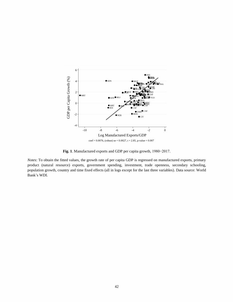
To understand the importance of manufactured exports to economic development, Fig. 1

displays relevant historical evidence in our sample of developing countries over the past three-

and-a-half decades. In the figure, each country has two observations for the log of manufactured

1 The Dutch disease refers to the coexistence of booming and lagging tradable goods sectors in a resource-rich

economy that generally suffers from low economic growth despite its large endowment of raw commodities. The

disease can arise from various forms of shocks such as a large natural resource discovery, a rise in the commodity

price, or large inflows of foreign aid or remittances. For seminal articles in this topic, see Corden and Neary (1982)

and Corden (1984) for theoretical developments and Sachs and Warner (1995, 1999, 2001) for supporting empirical

evidence. Also, see Frankel (2010), van der Ploeg (2011), and Magud and Sosa (2013) for an extensive review of the

literature, and Harding and Venables (2016) for a recent empirical exploration.

2

exports (as a ratio to GDP) and the growth rate of per capita GDP, which are averages for each

period, 1980−1999 and 2000−2017, so that we can trace their temporal changes within the

economy. From the illustration, we detect an apparent positive relationship between those two

variables in our sample when other standard growth determinants are also controlled. In line with

this observation, Hausmann et al. (2007), Jones and Olken (2008), Johnson et al. (2010), Berg et

al. (2012), and Sheridan (2014) argue that growth accelerations are strongly associated with

expansions of the manufacturing export sector.2

[Insert Fig. 1 here]

The result in Fig. 1 suggests that developing countries with heavy reliance on primary

commodity products may have an incentive to diversify their economies with an expansion of the

manufacturing sector that provides momentum for long-run economic growth. The main purpose

of this paper is to explore how those countries may achieve such a development objective by

managing their capital accounts and real exchange rate behavior.

Building on a simple static open macroeconomic model by Obstfeld and Rogoff (1996),

we first present the theoretical underpinnings of the economic structure in a commodity-

abundant country that is assumed to produce exportable commodities and manufactured goods as

well as nontraded goods. In such an economy, a rise in the world price of the country’s

commodity exports tends to appreciate its real exchange rate, whose reaction magnitude depends

on the degree of capital account openness.

The theoretical framework generates two testable hypotheses: First, capital controls

2 In a related vein, Dabla-Norris et al. (2010) show that the impact of foreign direct investment (FDI) on economic

growth is significantly positive only for countries with more diversified economic structures (i.e., lower dependence

on commodity exports).

3

mitigate the transmission of commodity price shocks to the real exchange rate. Second, capital

controls reduce the propensity to crowd out manufactured exports resulting from a commodity

price boom.

To explicitly test these hypotheses, we undertake a systematic panel data analysis based

on a sample of 37 non-oil commodity-exporting developing countries over the years from 1980

to 2017. Using the export volumes of 58 primary commodities and their global prices, we first

construct a country-specific real commodity price index as in Cashin et al. (2004) and Chen and

Lee (2018). We then show that commodity prices and real exchange rates are cointegrated and

exhibit a strong long-run comovement in our sample countries. In addition, we find statistically

significant evidence that capital controls, especially on FDI inflows (most likely toward the

commodity industries), help avoid a sharp real appreciation following a surge in commodity

prices.

Recognizing commodity prices as a driving force in the evolution of real exchange rates,

we find that capital account restrictions tend to shield manufactured exports by reducing the real

appreciation pressures stemming from a steep increase in commodity prices. In support of capital

controls’ positive role of preserving export competitiveness, we also report that the more

excessive the commodity currency appreciation or real overvaluation, the worse the export

performance of manufacturing. These results suggest the countercyclical use of capital controls

in countries whose currency values are strongly tied to their commodity export prices to lower

the intensity of the Dutch disease.

Our baseline results are robust to using alternative measures of capital controls based on

de jure and hybrid financial openness indices and controlling for exchange rate regimes and

major financial crises.

4

This paper contributes to a vast literature on the Dutch disease and real exchange rate in

the following three ways. First, we disentangle the dynamics of the Dutch disease into two key

links—one from commodity prices to real exchange rates and the other from the real exchange

rates to manufactured exports—and jointly address them in this paper. These relationships have

typically been studied separately in the prior literature. For example, the first link has been

analyzed in the commodity currency literature, such as Amano and van Norden (1995), Chen and

Rogoff (2003), Cashin et al. (2004), Coudert et al. (2011), Ricci et al. (2013), Bodart et al. (2012,

2015), and Chen and Lee (2018). The second link has been investigated by Grobar (1993),

Sekkat and Varoudakis (2000), Prasad et al. (2007), and Rajan and Subramanian (2011), who

report the damaging influence of real exchange rate uncertainty or misalignment. Unlike these

studies, we examine the impacts of commodity price shocks on manufactured exports, with the

degree of real exchange rate reaction determining the severity of the Dutch disease.

Second, our findings enrich the debate in the literature regarding how effective capital

controls are at managing unfavorable real exchange rate movements. Bodart et al. (2015) find

that, contrary to our results, an increase in commodity prices is related to stronger real

appreciation when a country has a less open capital account. Magud et al. (2018) survey close to

40 empirical studies and conclude that capital controls may help retain monetary autonomy and

alter the composition of capital flows; however, there are only a few successful cases in reducing

real appreciation pressures: in Chile, Malaysia, and Thailand. By contrast, Erten and Ocampo

(2016) find that capital account regulations are useful to decrease a real appreciation in emerging

economies. Similarly, some studies find that developing countries with higher capital account

openness are more likely to experience real overvaluation (Prasad et al., 2007) or less

undervaluation (Rodrik, 2008). The present paper complements this last strand of the literature.

5

Relative to the prior work, however, we emphasize the role of capital controls in limiting the

transmission of commodity price changes into the real exchange rate, a particularly relevant

concern for commodity-rich developing countries.

Third, we attempt to extend the Dutch disease literature using a sample of non-oil

commodity exporters and their export price movements as a source of foreign exchange windfall

shocks.3 Using such external shocks provides clear identification advantages in the empirical

models of the Dutch disease. This can be justified by the notion that the world commodity price

dynamics are driven mostly by global supply and demand conditions and can serve as an

exogenous terms-of-trade shock to the vast majority of commodity exporters (Chen et al., 2010).

As such, in contrast to the regression models that address a link between remittances and the real

exchange rate (e.g., Amuedo-Dorantes and Pozo, 2004; Lartey et al., 2012) or foreign aid flows

and economic growth (e.g., Rajan and Subramanian, 2005, 2008), it is less likely that our models

suffer from a potential endogeneity bias.4

As is widely known, international financial integration can offer various macroeconomic

benefits. For example, portfolio equity or debt inflows can relieve the financing constraints of

developing countries that otherwise face the high cost of capital with limited borrowing sources.

FDI inflows can bring along state-of-the-art technologies and managerial skills and improve

market accessibility. Growing financial integration also increases diversification opportunities

for both domestic and foreign investors.

Nevertheless, our findings indicate that countercyclical capital controls appear to be a

desirable policy toolkit in commodity-exporting developing countries to effectively manage real

3 Similar to our work, Ismail (2010) evaluates the Dutch disease effects of permanent oil price shocks using a small

set of oil-exporting countries.

4 In the earlier literature, reverse causality was a potential concern because “migrants usually look at exchange rates

in order to decide how much to remit back home” (Lartey et al., 2012); and “aid flows could go to countries that are

doing particularly badly, or to countries that are doing well” (Rajan and Subramanian, 2008).

6

appreciation pressures arising from their export price booms and to implicitly subsidize

economic diversification.5,6 In line with this view, Aizenman et al. (2007) and Prasad et al. (2007)

insist that higher ratios of self-financing may spur faster growth when nonindustrial countries do

not have adequate capacity to absorb foreign resources due to unstable macroeconomic policies

and economic structures that are vulnerable to overvaluations.

In the next section, we present a simple small open economy model and derive two

testable hypotheses. Section 3 describes the data and empirical model specifications. The

baseline estimation results and robustness analyses are reported in Section 4, and finally, Section

5 concludes.

2. A theoretical framework

This section presents a three-sector small open economy model that highlights the

transmission of commodity price shocks to the real exchange rate and the resulting response in

exports of manufactured goods. The model builds on the canonical framework of Obstfeld and

Rogoff (1996, Ch. 4), with relevant implications taken from Corden and Neary (1982) and

Bodart et al. (2015).

For our purposes, we assume that all of the commodity goods produced by the home

country are exported abroad, but the foreign country in the model is not involved in commodity

5 In fact, imposing capital controls can avoid selecting beneficiaries for export subsidies and uniformly provide an

economy-wide incentive to all exporting industries.

6 For capital controls and their role as a macroprudential policy, see the recent surveys provided in Engel (2016) and

Erten et al. (forthcoming).

7

trading at all. As is standard in the literature, we let global commodity prices be determined by

the world market conditions and thus exogenously be given to the domestic commodity sector.

The parsimonious model structure enables us to derive three propositions, which form the

basis of our main hypotheses. The detailed model derivations can be found in Appendix E.

2.1. Production

Consider that the domestic economy produces three types of goods: exportable

commodities or resources (𝑅), exportable manufactured goods (𝑀), and nontraded (𝑁) goods.

The production function in each sector exhibits constant returns to scale and is given by

𝑌𝑅 = 𝐴𝑅𝐿𝑅𝛼 𝐾𝑅

1−𝛼, (1)

𝑌𝑀 = 𝐴𝑀𝐿𝑀𝛽

𝐾𝑀1−𝛽

, (2)

𝑌𝑁 = 𝐴𝑁𝐿𝑁, (3)

where 𝐴𝑖, 𝐿𝑖, and 𝐾𝑖 are the total factor productivity, labor, and capital stock employed in the

production of sector 𝑖 = 𝑅, 𝑀, 𝑁, respectively. Note that both capital and labor are required in the

production of tradable goods, with 𝛼 and 𝛽 capturing the labor share. The nontraded goods’

production is assumed to rely on labor as the only input.

In the benchmark case, we assume that capital is perfectly mobile internationally and

labor is mobile only domestically. Thus, the domestic marginal product of capital is given by the

world interest rate 𝑟∗ , while perfect domestic labor mobility ensures that the wage rate 𝑤 is

8

equalized across sectors. Like Obstfeld and Rogoff (1996), we allow a common rate of

productivity shocks in the exportable sectors.

Under the assumptions above, combining log-differentiated profit-maximization

conditions in three sectors gives

��𝑁 = 𝜏(��𝑅 − ��𝑀) − ��𝑁 (4)

with 𝜏 = 1 (𝜇𝐿,𝑅 − 𝜇𝐿,𝑀)⁄ ,

where 𝑝𝑖 is the price of goods in sector 𝑖; 𝜇𝐿,𝑖 is the labor income share (0 < 𝜇𝐿,𝑖 < 1), defined

as 𝜇𝐿,𝑖 ≡ 𝑤𝐿𝑖/𝑝𝑖𝑌𝑖; and a hat above the variable denotes a logarithmic derivative, �� = d(ln 𝑥).

Note that as long as the commodity sector is more labor-intensive than manufacturing, we have

𝜏 > 0.7 The underlying mechanism in Eq. (4) is that higher commodity prices (relative to prices

in the manufacturing sector) raise the demand for labor and the wage rate in the commodity

sector. This in turn causes a shift of labor out of the other sectors and an increase in the overall

wage rate, eventually boosting the price of labor-intensive nontraded goods.

2.2. Consumption

The representative domestic household in our model economy consumes two types of

goods: nontraded and manufactured products. Accordingly, a domestic consumer’s utility

function takes the following Cobb-Douglas form:

7 Equivalently, the manufacturing sector is assumed to be more capital-intensive than the commodity sector. This

assumption is needed to replicate the main logic of the resource movement effect that follows (as in Corden and

Neary, 1982).

9

𝑈 = 𝛾𝐶𝑁𝜃𝐶𝑀

1−𝜃, (5)

where 𝐶𝑁 and 𝐶𝑀 are the consumption of the two goods, 𝜃 is the share of nontraded goods in the

domestic household’s consumption basket, and 𝛾 = 𝜃−𝜃(1 − 𝜃)−(1−𝜃).

Similarly, the representative household in the foreign country consumes the nontraded

goods as well as imported manufactured goods that are produced by the home country. These

two goods are not perfect substitutes for foreign consumers. A foreign household shows the

following preferences:

𝑈∗ = 𝛾∗𝐶𝑁∗𝜃∗

𝐶𝑀∗1−𝜃∗

, (6)

where 𝛾∗ = 𝜃∗−𝜃∗(1 − 𝜃∗)−(1−𝜃∗) and a superscript asterisk on the variable denotes a foreign

value.

Note that since the supply of nontraded goods satisfies the domestic demand and the

labor supply is fixed in the domestic factor market, the market clearing conditions in the home

country are given by

𝑌𝑁 = 𝐶𝑁, (7)

𝐿 = 𝐿𝑅 + 𝐿𝑀 + 𝐿𝑁. (8)

2.3. Real exchange rate

In the absence of any frictions in international trade, the law of one price is assumed to

hold in the long run for the tradable goods so that

10

𝐸𝑝𝑖 = 𝑝𝑖∗ for 𝑖 = 𝑀, 𝑅, (9)

where 𝐸 is the nominal exchange rate, defined as the price of domestic currency in terms of

foreign currency, and 𝑝𝑖 and 𝑝𝑖∗ are the domestic and foreign currency prices of tradable good 𝑖,

respectively.

Using the consumption-based price index for the home and foreign economies and the

law of one price for tradable goods, we can express the real exchange rate (𝑄), the relative price

of the domestic consumption basket in terms of the foreign consumption basket, as follows:

𝑄 =𝐸𝑃

𝑃∗=

𝐸𝑝𝑁𝜃𝑝𝑀

1−𝜃

(𝑝𝑁∗ )𝜃∗(𝑝𝑀

∗ )1−𝜃∗ , (10)

where 𝑃 and 𝑃∗ are domestic and foreign aggregate price indices, respectively. By construction,

an increase in 𝑄 indicates a real appreciation of the home currency relative to the foreign

currency.

2.4. Model implications

This subsection summarizes three propositions that emerge from the model.

Proposition 1. An increase in world prices of commodities induces real appreciation in a

commodity-exporting country.

11

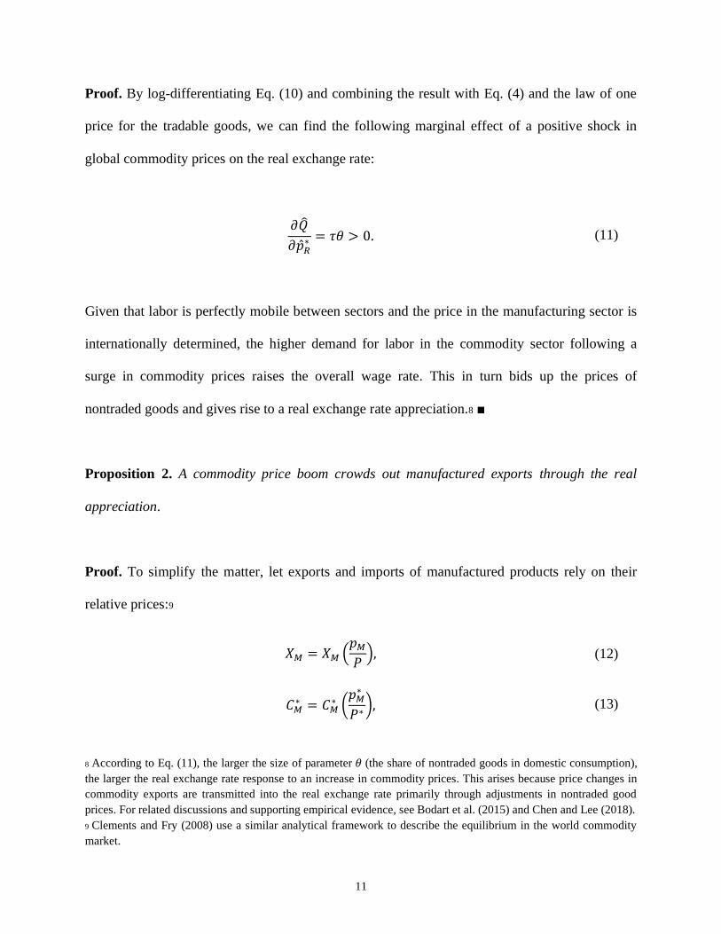
Proof. By log-differentiating Eq. (10) and combining the result with Eq. (4) and the law of one

price for the tradable goods, we can find the following marginal effect of a positive shock in

global commodity prices on the real exchange rate:

𝜕��

𝜕��𝑅∗ = 𝜏𝜃 > 0. (11)

Given that labor is perfectly mobile between sectors and the price in the manufacturing sector is

internationally determined, the higher demand for labor in the commodity sector following a

surge in commodity prices raises the overall wage rate. This in turn bids up the prices of

nontraded goods and gives rise to a real exchange rate appreciation.8 ■

Proposition 2. A commodity price boom crowds out manufactured exports through the real

appreciation.

Proof. To simplify the matter, let exports and imports of manufactured products rely on their

relative prices:9

𝑋𝑀 = 𝑋𝑀 (𝑝𝑀

𝑃), (12)

𝐶𝑀∗ = 𝐶𝑀

∗ (𝑝𝑀

∗

𝑃∗), (13)

8 According to Eq. (11), the larger the size of parameter 𝜃 (the share of nontraded goods in domestic consumption),

the larger the real exchange rate response to an increase in commodity prices. This arises because price changes in

commodity exports are transmitted into the real exchange rate primarily through adjustments in nontraded good

prices. For related discussions and supporting empirical evidence, see Bodart et al. (2015) and Chen and Lee (2018).

9 Clements and Fry (2008) use a similar analytical framework to describe the equilibrium in the world commodity

market.

12

where the definition of manufactured exports is given by subtracting domestic consumption from

production such that 𝑋𝑀 ≡ 𝑌𝑀 − 𝐶𝑀 . Since the two countries, home and foreign, determine

market forces, the world market clears when 𝑋𝑀 = 𝐶𝑀∗ . By log-differentiating this market-

clearing condition, combined with the law of one price for tradable manufacturing sector and the

definition of the real exchange rate, we find

(𝑝𝑀

∗

𝑃∗

) = 𝜂��, (14)

where 𝜂 = 휀𝑠/(휀𝑠 − 휀𝑑), 휀𝑠(≥ 0) is the price elasticity of manufacturing supply, and 휀𝑑(≤ 0) is

the price elasticity of manufacturing demand. Since 0 ≤ 𝜂 ≤ 1 , Eq. (14) shows a positive

relationship between the foreign relative price of manufactured goods and the real exchange rate.

Now, combining a log-differentiated version of Eq. (13) with Eq. (14), we can derive Eq. (15),

which demonstrates a decline in the home country’s manufactured exports in response to rising

global commodity prices, with the size of damage positively depending on the degree of real

appreciation:

𝜕��𝑀∗

𝜕��𝑅∗ = 휀𝑑𝜂 (

𝜕��

𝜕��𝑅∗ ) ≤ 0, (15)

where 𝜕�� 𝜕��𝑅∗⁄ > 0 by Eq. (11). ■

An intuitive interpretation of Eq. (15) is that a surge in commodity prices is expected to

increase the domestic input costs (i.e., wage rates) of producing manufactured goods and squeeze

manufacturers’ profits, thereby reducing their incentives for production. The lower supply is then

followed by a rise in the price of manufactured exports, adversely affecting the foreign demand.

13

Proposition 3. Capital controls restrict the magnitude of the real exchange rate response to a

commodity price shock.

Proof. Deviating from the benchmark model assumption, let us now consider an extreme case of

capital market autarky to study the effect of capital controls. With no cross-border capital flows,

the return to capital 𝑟 is endogenously determined in the domestic capital market. Resolving the

model with only domestically mobile capital and labor, we find the following real exchange rate

response to a commodity price shock:

𝜕��

𝜕��𝑅∗ = 𝜑𝜃 > 0

(16)

with 𝜑 = 1/(𝜇𝐿,𝑅 − (𝜇𝐾,𝑅/𝜇𝐾,𝑀)𝜇𝐿,𝑀),

where 𝜇𝐾,𝑖 is the capital income share (0 < 𝜇𝐾,𝑖 < 1), defined as 𝜇𝐾,𝑖 ≡ 𝑟𝐾𝑖/𝑝𝑖𝑌𝑖 in sector 𝑖. By

comparing Eqs. (11) and (16), we observe that the real exchange rate reaction is smaller in the

presence of capital controls because 𝜑 < 𝜏.10 ■

This result occurs because a given rise in commodity prices boosts the rental rate for

capital as well as the wage rate when cross-border capital movement is restricted, making the

resulting increase in the wage rate smaller than would be the case with free international capital

mobility (see Eqs. (E.7) and (E.13) in Appendix E). As a result, the price of nontraded goods will

increase less under the capital control, mitigating the appreciation pressures of the real exchange

rate.

10 Note that 𝜇𝐾,𝑅 < 𝜇𝐾,𝑀 due to the assumption in Footnote 7.

14

2.5. Testable hypotheses

Combining Propositions 1 and 3 above, our first testable hypothesis is:

Hypothesis 1. Capital controls lessen the transmission of commodity price shocks to the real

exchange rate.

Moreover, combining Propositions 2 and 3 above, the second testable hypothesis is:

Hypothesis 2. Capital controls lower the propensity to crowd out manufactured exports arising

from a commodity price boom.

In the next section, we build empirical models to test the above two hypotheses using a

panel dataset.

3. Data and empirical model specification

Our sample covers 37 non-oil commodity-exporting countries for the period of

1980−2017. See Appendix A for a full list of sample countries. Major energy exporters,

especially oil exporters, are not part of our sample because of their highly volatile export prices

and various strategic pricing behaviors (e.g., possible collusion among OPEC countries), which

can complicate their economies’ transmission mechanisms between resource export prices and

15

real exchange rates. In fact, almost all of the large oil-exporting countries peg their currencies to

the dollar and do not allow nominal exchange rate adjustments to an external shock.

For our purpose, we keep commodity-dependent countries with a non-negligible share of

manufactured exports, so in the vast majority of our sample countries, at least 5% of their total

exports are manufactured products.

In the rest of the section, we briefly explain the definition and source of the variables

used in our empirical analysis and then present the baseline regression models.

3.1. Key variables

3.1.1. Real exchange rate

We use the CPI-based real effective exchange rate, which is the average of the bilateral

real exchange rates between a country and its trading partners weighted by the respective trade

shares of each trading partner. It is measured such that the higher index indicates the real

appreciation of the domestic currency. The monthly and annual real effective exchange rate

series are taken from the Bruegel database released by Darvas (2012).

3.1.2. Real commodity price

The real commodity price index is defined as the world (nominal) price index of a

country’s commodity exports relative to the world price index of manufactured goods exports.

Following Cashin et al. (2004) and Chen and Lee (2018), we construct a country-specific real

commodity price index using 58 commodities as follows:11

11 For a complete list of commodities, see Appendix A.

16

𝑅𝐶𝑃𝑖𝑡 = [∑ 𝑤𝑖𝑗(ln 𝑝𝑗𝑡)𝐽𝑗=1 ] 𝑀𝑈𝑉𝑡⁄ (17)

with 𝑤𝑖𝑗 = (1/𝑇 ∑ 𝑒𝑥𝑖𝑗,𝑡𝑇𝑡=1 ) (1/𝑇 ∑ 𝐸𝑋𝑖𝑡

𝑇𝑡=1 )⁄

where 𝑝𝑗𝑡 is the global price of commodity j at time t, 𝑀𝑈𝑉𝑡 is the unit value index of

manufactured exports for 20 industrial economies, 𝑒𝑥𝑖𝑗,𝑡 is country i’s export volume (in U.S.

dollars) of commodity j, and 𝐸𝑋𝑖𝑡 is the volume of the total commodity exports of country i. We

keep weight 𝑤𝑖𝑗 constant over time to eliminate the quantity effect from the price index

calculation.12 Whenever necessary, we take the average of monthly commodity price indices in

each year to convert them to an annual frequency.

The monthly world commodity price series are extracted from the International Monetary

Fund (IMF) and World Bank’s Pink Sheet data, the unit value index of manufactured exports

from the IMF’s International Financial Statistics, and the annual commodity trade data from the

UN COMTRADE database.

3.1.3. Capital controls

For the baseline regression analysis, we build a capital control variable based on an

annual de facto international financial integration taken from the updated External Wealth of

Nations Mark II database available in Lane and Milesi-Ferretti (2017). Among the integration

indicators proposed by Lane and Milesi-Ferretti (2003), we adopt a measure of cross-border

equity holdings that is defined as follows:

𝐺𝐸𝑄𝑖𝑡 = (𝐸𝑄𝑖𝑡𝐴 + 𝐹𝐷𝐼𝑖𝑡

𝐴 + 𝐸𝑄𝑖𝑡𝐿 + 𝐹𝐷𝐼𝑖𝑡

𝐿 )/𝐺𝐷𝑃𝑖𝑡 (18)

12 More specifically, we use the period-average values of export volume of each commodity over the period of

1986−2010.

17

where 𝐸𝑄𝑖𝑡 and 𝐹𝐷𝐼𝑖𝑡 are respectively country i’s stocks of portfolio equity and foreign direct

investment at time t, with the superscript 𝐴 indicating assets, and the superscript 𝐿, liabilities. A

higher value of 𝐺𝐸𝑄 in Eq. (18) represents a more open capital account.

We limit our attention to the equity-based measure to be broadly consistent with the

model environment in our theoretical framework, excluding debt instruments and foreign

exchange reserves. In fact, as noted by Kose et al. (2009), debt flows tend to be highly volatile

and can magnify the negative impact of adverse shocks in developing economies.13 In order to

create a capital control indicator, we take the inverse of 𝐺𝐸𝑄 so that a higher value of the

indicator (= 1/𝐺𝐸𝑄) corresponds to stricter restrictions on capital flows.14

The considerable time variation for de facto capital controls at the country level makes

them preferable to de jure measures, as it helps identify the intended effect of capital market

regulations in our panel fixed-effect regressions. The de facto indicators also allow us to

distinguish between controls on capital inflows and controls on capital outflows during the

sample period.

3.1.4. Manufactured exports

We use manufactured exports as a share of GDP. The annual data are taken from the

World Bank’s World Development Indicators (WDI).

13 Kose et al. (2009) also acknowledge that de facto financial openness measures tend to better capture the extent of

a country’s integration into global financial markets than de jure ones because the latter cannot capture the degree of

enforcement and effectiveness of capital controls.

14 To mitigate the influence of outliers, we drop the top 1% (inclusive) of observations for capital controls before

conducting a regression analysis.

18

3.2. Other variables

Other control variables in our empirical analysis include government spending (the log of

the ratio of government consumption to GDP), trade openness (the log of the sum of exports and

imports relative to GDP), and investment (the log of the ratio of gross capital formation to GDP).

We obtain the information for these variables from the World Bank’s WDI.

In addition, since sectoral output and employment data are not available for the bulk of

our sample countries, we follow Lane and Milesi-Ferretti (2004) and define relative GDP per

capita as the trade-weighted sum of the log of the home country’s GDP per capita relative to its

trading partners’. It is included to capture relative output levels and control for a Balassa–

Samuelson effect in the real exchange rate regressions. Bilateral trade data are collected from the

IMF’s Direction of Trade Statistics and GDP per capita in constant 2010 U.S. dollars from the

World Bank’s WDI.

Lastly, in order to control for the effect of foreign demand in the manufactured export

regressions, we create foreign income as the trade-weighted sum of the log of trading partners’

GDP per capita. Summary statistics for all variables are presented in Appendix Table B.1.

3.3. Baseline regression model specifications

As a preliminary procedure, we apply the standard panel time-series tests to our dataset

and find the presence of non-stationarity for all annual variables including the real exchange rate

and real commodity price indices. We also find evidence of cointegration among the annual

variables at the conventional significance level (results available in Appendix Tables C.1 and

19

C.2). Accordingly, we employ a panel version of the dynamic ordinary least squares (DOLS)

estimator to efficiently estimate the long-run cointegrating relationship, which uses a parametric

correction for endogeneity by including the leads and lags of the first difference of each

regressor.15

Kao and Chiang (2000) provide evidence that DOLS is superior to the fully modified

ordinary least squares (FMOLS) estimator, another widely used methodology, in removing a

finite sample bias associated with endogeneity as well as serial correlation. Note also that

FMOLS requires a balanced panel, and our estimation would have to rely on a substantially

reduced sample size.

For country i and year t, the first baseline regression model takes the following panel

DOLS(1,1) specification:

𝑅𝐸𝑅𝑖𝑡 = 𝛼1𝑅𝐶𝑃𝑖𝑡 + 𝛼2(𝑅𝐶𝑃𝑖𝑡 × 𝐾𝐶𝑖𝑡) + 𝛼3𝐾𝐶𝑖𝑡 + 𝑿𝒊𝒕𝜸

+ ∑ Δ𝒁𝒊,𝒕+𝒋𝜹𝒋1𝑗=−1 + 𝜙𝑖 + 𝜙𝑡 + 휀𝑖𝑡

(19)

where 𝑅𝐸𝑅𝑖𝑡 is the log of the real effective exchange rate; 𝑅𝐶𝑃𝑖𝑡 is the log of the real commodity

price index; 𝐾𝐶𝑖𝑡 is a measure of capital control; 𝑿𝒊𝒕 is a vector of additional fundamental

determinants, including government spending, relative GDP per capita, and trade openness; 𝒁𝒊𝒕

is a vector of all continuous explanatory variables; 𝜙𝑖 is a country fixed effect; 𝜙𝑡 is a time fixed

effect; 휀𝑖𝑡 is a residual; and Δ is the first-difference operator. By controlling for country and time

fixed effects, the problem of omitted variables bias or misspecification is diminished. To account

15 As noted by Lane and Milesi-Ferretti (2004), “the superconsistency property of cointegrated equations means that

any possible endogeneity running from the real exchange rate to the regressors does not affect the estimated long-

run coefficients.”

20

for potential cross-sectional correlation as well as autocorrelation and heteroscedasticity, we use

Driscoll and Kraay’s (1998) standard errors for statistical inferences.

Our Hypothesis 1 tests whether 𝛼1 > 0 and 𝛼2 < 0 in Eq. (19) so that the positive impact

of RCP shock on RER (or the RCP elasticity of RER) may be reduced through restrictions on

cross-border capital movements. Regarding other control variables, government consumption is

typically spent on nontraded goods, and we expect a positive coefficient for government

spending. Due to the Balassa–Samuelson effect, relative GDP per capita is expected to enter the

RER regression with a positive sign. Trade openness tends to increase the share of tradable goods

in domestic consumption, so we expect it to have a negative effect on RER.

The second baseline regression model takes the following panel fixed-effect estimator:

𝑀𝑋𝑖𝑡 = 𝛽1𝑅𝐶𝑃𝑖𝑡 + 𝛽2(𝑅𝐶𝑃𝑖𝑡 × 𝐾𝐶𝑖𝑡) + 𝛽3𝐾𝐶𝑖𝑡 + 𝒀𝒊𝒕𝜸 + 𝜙𝑖 + 𝜙𝑡 + 𝑒𝑖𝑡 (20)

where 𝑀𝑋𝑖𝑡 is the log of the ratio of manufactured exports to GDP in country i at time t, and 𝒀𝒊𝒕

is a vector of other potential determinants of country i’s exports of manufacturing, including

trade openness, investment, and foreign income.

In order to focus on the long-run effects of commodity price movements on manufactured

exports, we smooth out the business cycle fluctuations by transforming the annual frequency data

into five-year averages, as is standard in the growth literature (e.g., Rodrik, 2008; Aghion et al.,

2009).

Our Hypothesis 2 tests whether 𝛽1 < 0 and 𝛽2 > 0 in Eq. (20) so that the negative impact

of RCP shock on MX may be moderated through restrictions on international capital movements.

Regarding the other regressors, a greater value of investment is likely to promote MX owing to an

increase in available physical capital, which may be required for manufacturing production. The

21

higher level of trade openness is usually associated with lower trade barriers in tariffs and quotas,

likely boosting a country’s foreign trade, including MX. The demand for domestically produced

manufactured goods would increase with trading partners’ purchasing power, so foreign income

is expected to show a positive sign.

4. Empirical results

4.1. Main results

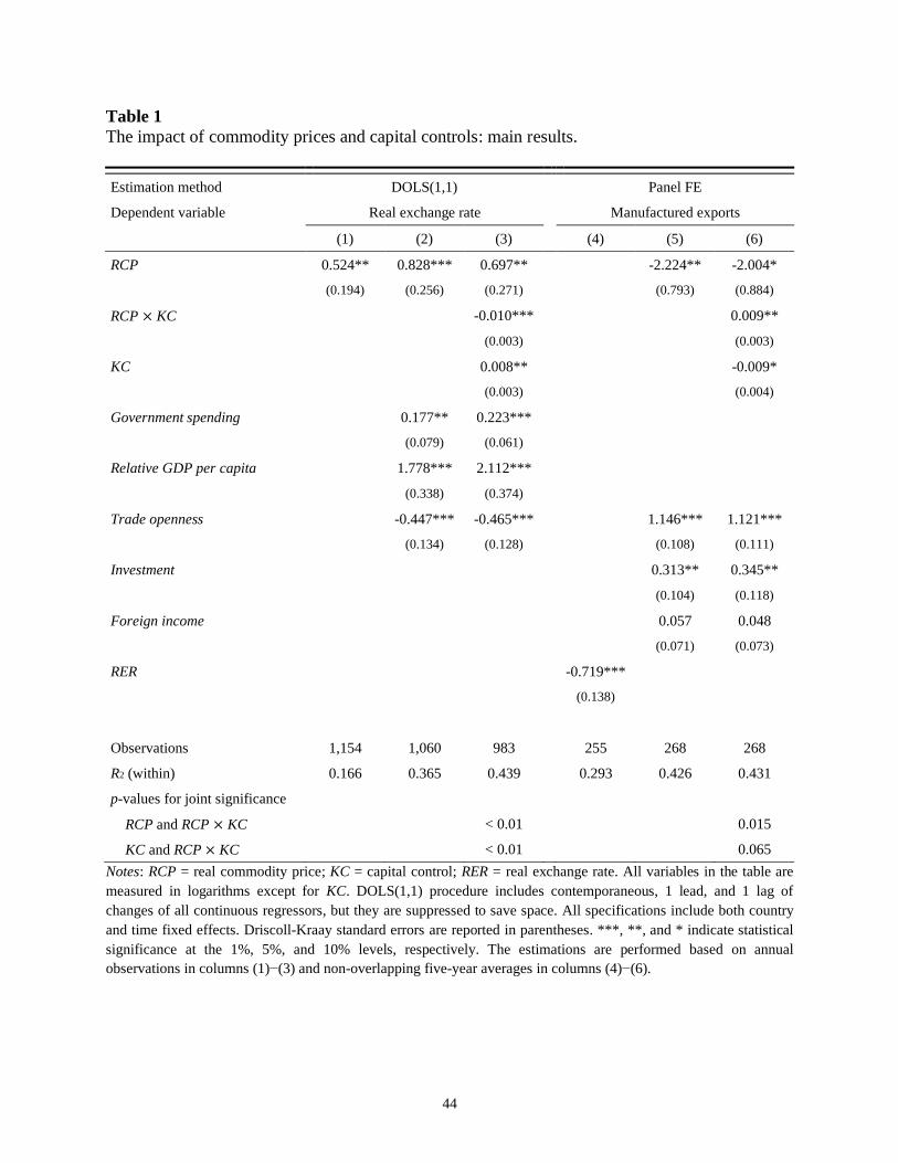
Columns (1)−(3) of Table 1 present the estimation results based on our first baseline

regression model in Eq. (19). The main parameters of our interest are on the coefficients of the

commodity price index RCP and its interaction with capital controls RCP × KC.

[Insert Table 1 here]

Column (1) displays a significantly positive coefficient for RCP, which demonstrates its

long-run cointegrating relationship with RER in our sample countries. This result reinforces the

previous empirical evidence for the commodity currency phenomenon documented in Chen and

Rogoff (2003), Cashin et al. (2004), Coudert et al. (2011), Ricci et al. (2013), Bodart et al. (2012,

2015), and Chen and Lee (2018).

Column (2) extends the specification with additional fundamental determinants of RER,

including government spending, relative GDP per capita, and trade openness. We confirm a

22

positive long-run relationship between RCP and RER, with expected signs for the other control

variables. Indeed, inclusion of the other RER determinants strengthens the magnitude of RCP

elasticity and its statistical significance.

In column (3), we further extend the model with KC and its interaction with RCP.16

Significantly positive RCP and negative RCP × KC coefficient estimates indicate that while an

increase in commodity prices induces real appreciation, a more stringent capital control (a higher

value of KC) appears to reduce the size of appreciation, in support of our Hypothesis 1. In

particular, a 1% rise in RCP would lead to long-run real appreciation of 0.56% when KC is at its

sample average and appreciation of 0.37% when there is a one–standard deviation increase in KC

above its mean value.17

Turning to the MX regressions, we first show in column (4) a statistically significant and

negative response of MX to RER appreciation, consistent with the conventional theory. The

negative coefficient estimate of RER indicates that a 1% increase in RER tends to lower MX by

0.72% in our sample countries.

We now introduce RCP as a determinant of MX while controlling for other relevant

variables. As shown in column (5), a significantly negative RCP coefficient provides empirical

evidence for the Dutch disease, the coexistence of a commodity boom and manufacturing

shrinkage, in commodity-exporting developing countries.18 Other control variables such as trade

16 Note that the source data for KC, the updated External Wealth of Nations Mark II database (Lane and Milesi-

Ferretti, 2017), is available up to 2015, so the specification that includes KC has a smaller sample size.

17 The net effects of a 1% increase in RCP are calculated by 𝛼1 + (𝛼2 × mean𝐾𝐶) and 𝛼1 + (𝛼2 × (mean𝐾𝐶 +

𝜎𝐾𝐶 )), respectively.

18 We have also considered a specification that includes both RER and RCP at the same time to test whether the

former drives out the effect of the latter in the MX regression. The estimation results, available upon request, show

that both variables keep their expected negative signs, but only RER remains strongly significant. This result verifies

the role of RER as an intermediate channel through which an RCP boom may hurt MX in developing countries.

23

openness, investment, and foreign income have the expected positive signs, although foreign

income is not significant at standard confidence levels.

Finally in column (6), we have a full specification, as in our second baseline regression

model in Eq. (20). A negative RCP coefficient and a positive coefficient for the interaction term

between RCP and KC lend support to our Hypothesis 2. Specifically, a 1% rise in RCP would

decrease MX by 1.89% when KC is at its sample average and by 1.73% when KC is at one

standard deviation above its mean value. In other words, capital flow regulations are expected to

slow down a manufacturing downturn in developing countries by resisting the appreciation

pressures associated with a commodity price boom.

The result in column (6) also shows that KC itself has a negative effect on MX, although

it is only marginally significant. Some plausible explanations for this result are as follows: higher

barriers on capital mobility can contract manufacturing production through a limited supply of

inputs in the foreign capital-dependent production process, or through foregone opportunities to

benefit from positive spillovers generated by FDI in the commodity sector. While the net effect

of tighter KC on MX is positive in our sample, the negative standalone effect of KC suggests that

a careful cost–benefit analysis across industries may precede the imposition of KC to exploit

foreign capital more effectively.19

In addition to individual coefficient estimates and their standard errors, Table 1 also

reports p-values for F-statistics to test the null hypothesis that RCP has no effect on RER and MX

in the interaction variable regressions. As seen in Eqs. (19) and (20), this null hypothesis requires

a joint significance test for RCP and its interaction with KC. The consistently low p-values

reported in columns (3) and (6) validate our baseline empirical specifications. Likewise, the

19 Using the result in column (6) of Table 1, the net effect of KC on MX can be evaluated by {exp[(𝛽2 × mean𝑅𝐶𝑃 ×

𝜎𝐾𝐶 ) + (𝛽3 × 𝜎𝐾𝐶 )] − 1} × 100.

24

relatively low p-values for a joint significance test for KC and its interaction with RCP provide

further support for the validity of our specifications.

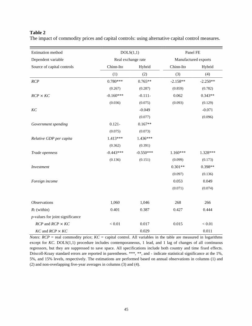
4.2. Alternative capital control indicators

In this subsection, we test whether our main results are sensitive to alternative measures

of capital controls. As a first exercise, we use Chinn and Ito’s (2006) index, which is one of the

most widely used de jure measures of capital account openness. It is built upon the information

about legal or regulatory barriers to international financial transactions reported in the IMF’s

Annual Report on Exchange Arrangements and Exchange Restrictions. As higher values of the

index represent more open capital markets, we define a capital control dummy variable that takes

a value of unity at time t if the Chinn–Ito index for a country is below the 20th percentile in our

sample and zero otherwise.20

In a second exercise, we employ the KOF hybrid financial globalization index, available

at the KOF Swiss Economic Institute (Gygli et al., 2019), which combines de facto and de jure

indices with equal weights.21 The de facto index is based on work of Lane and Milesi-Ferretti

(2007, 2017) and takes a quantity-based measure of stocks of foreign assets and liabilities. More

specifically, it consists of 27.6% international debt, 27.1% international income payments, 26.7%

FDI, 16.5% portfolio investment, and 2.1% international reserves. On the other hand, the de jure

index is based on the indicator developed by Chinn and Ito (2006) and the investment restrictions

published in the World Economic Forum Global Competitiveness Report. It is composed of 38.5%

capital account openness, 33.3% investment restrictions, and 28.2% international investment

20 We have also considered the 10th and 30th percentiles as alternative thresholds and found very similar results.

21 The original KOF globalization index was introduced by Dreher (2006) and later updated by Dreher et al. (2008).

25

agreements. Since a higher value of the index represents that an economy is more financially

globalized, we use the inverse of the KOF hybrid index as a measure of capital controls.

Table 2 reports the estimation results when we construct KC based on the Chinn–Ito

index in columns (1) and (3) and the KOF hybrid index in columns (2) and (4). Indeed, we find

that the interaction effect between RCP and KC retains the expected signs in all cases, though it

is not always statistically significant (the p-value for the interaction term is 0.53 in column (3)).

One of the reasons for the difficulty of identifying the interaction effect in column (3) is the

relatively little time variation in the Chinn–Ito index at the country level.

[Insert Table 2 here]

4.3. Robustness test controlling for exchange rate regimes and financial crises

In order to test the robustness of our main results, we introduce two more factors into the

baseline regression models. The goal is to see if the variable of our main interest, the interaction

of RCP and KC, continues to play an important role when controlling for other variables that

might affect the transmission of RCP changes to RER and MX.

The first variable we add is a country’s choice of a fixed vs. a flexible exchange rate

regime. To do so, we follow Ilzetzki et al. (2019) and define a “flexible regime” dummy variable

using their fine classification code. This dummy takes a value of one in a given year if the code

for a country is between 5 and 14, or zero if the code is below 5. In the case of five-year average

data, we first take the average of classification codes and then generate a binary regime variable

26

following the same rule. By construction, the reference category (i.e., flexible regime = 0) is a de

facto peg or preannounced horizontal band with margins of no larger than ±2%.22

From a theoretical point of view, even if the nominal exchange rate remains fixed in

pegged countries, a more stable real exchange rate in the long run will not be guaranteed because

a priori, we do not know how much domestic prices will react to spikes in commodity prices

relative to the reaction in nonpegged countries. For this reason, the impact of exchange rate

regimes is more of an empirical issue that deserves further investigation.

Columns (1) and (3) of Table 3 show the regression results when flexible regime and its

interaction with RCP are included as additional controls. First of all, we continue to see the

expected signs, with strong significance for the RCP and KC interaction variable, although the

inclusion of multiple interaction variables that may be highly correlated lessens the statistical

significance of the estimates for some of the regressors.

[Insert Table 3 here]

Moreover, in column (1), we find a significantly negative sign for RCP’s interaction with

flexible regime. This result reflects that a flexible nominal exchange rate provides a more

effective RER-stabilizing role in the long run for a country facing a commodity price boom, in

accordance with the findings of Bodart et al. (2015). Nevertheless, the interaction between RCP

and flexible regime does not necessarily help shield manufactured exports, as its coefficient

estimate in column (3) has a negative sign although it is not statistically significant.

22 We exclude episodes of “Dual market in which parallel market data is missing” (fine classification code = 15)

from the sample for regression analysis.

27

The second factor we introduce is a major financial crisis that developing countries in our

sample have undergone during the sample period. We create a “crisis” variable that reflects

country-level banking crises as well as the 2008−09 global financial crisis and define it as the

sum of crisis years divided by the number of years in the corresponding period. Hence, for the

annual data, crisis is a dummy variable to capture a crisis year. It intends to capture severe

financial market instability that has the potential to cause large changes for our dependent

variables. The information for the banking crisis years comes from the World Bank’s Global

Financial Development database.

Columns (2) and (4) of Table 3 report the results when controlling for the interaction

between RCP and crisis. While we find no significant effects of the financial crisis on the

transmission of RCP changes into RER and MX, the RCP and KC interaction effects stay

significant with the expected signs, confirming the robustness of our main results.

4.4. Quantile regression evidence for nonlinearity

The main focus of our analysis is on the Dutch disease resulting from a commodity price

boom, so we looked into two relationships in Tables 1−3: one between RCP and RER, and the

other between RCP and MX, with KC playing a dampening role in both relationships. By the

model’s design, the operative channel through which a country suffers from the Dutch disease is

the extent of its real appreciation.

In this subsection, we test the possible nonlinearity between commodity currency

responses and their impact on manufactured exports using the following quantile regression

model:

28

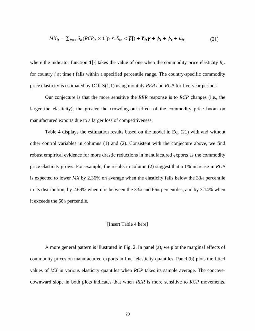
𝑀𝑋𝑖𝑡 = ∑ 𝛿𝑘(𝑅𝐶𝑃𝑖𝑡 × 𝟏[p ≤ 𝐸𝑖𝑡 < p])𝑘=1 + 𝒀𝒊𝒕𝜸 + 𝜙𝑖 + 𝜙𝑡 + 𝑢𝑖𝑡 (21)

where the indicator function 𝟏[∙] takes the value of one when the commodity price elasticity 𝐸𝑖𝑡

for country i at time t falls within a specified percentile range. The country-specific commodity

price elasticity is estimated by DOLS(1,1) using monthly RER and RCP for five-year periods.

Our conjecture is that the more sensitive the RER response is to RCP changes (i.e., the

larger the elasticity), the greater the crowding-out effect of the commodity price boom on

manufactured exports due to a larger loss of competitiveness.

Table 4 displays the estimation results based on the model in Eq. (21) with and without

other control variables in columns (1) and (2). Consistent with the conjecture above, we find

robust empirical evidence for more drastic reductions in manufactured exports as the commodity

price elasticity grows. For example, the results in column (2) suggest that a 1% increase in RCP

is expected to lower MX by 2.36% on average when the elasticity falls below the 33rd percentile

in its distribution, by 2.69% when it is between the 33rd and 66th percentiles, and by 3.14% when

it exceeds the 66th percentile.

[Insert Table 4 here]

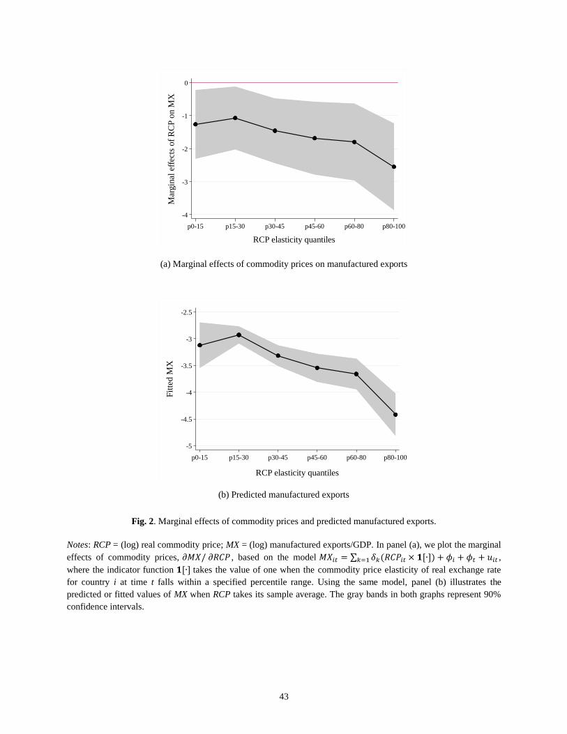
A more general pattern is illustrated in Fig. 2. In panel (a), we plot the marginal effects of

commodity prices on manufactured exports in finer elasticity quantiles. Panel (b) plots the fitted

values of MX in various elasticity quantiles when RCP takes its sample average. The concave-

downward slope in both plots indicates that when RER is more sensitive to RCP movements,

29

there is a more severe crowding-out effect on MX given a commodity price shock. 23 This

observation, in combination with the main results in Table 1, suggests the countercyclical use of

capital controls in countries whose currency values strongly co-move with their commodity

export prices in order to protect non-commodity tradable sectors.

[Insert Fig. 2 here]

4.5. Real exchange rate misalignments and manufactured exports

Although our interpretations have focused on the case of real appreciations, the results

presented thus far do not reveal a possible asymmetry in MX responses following changes in

RER. We thus investigate the cases for under- and overvaluations of RER relative to its

equilibrium levels and their possibly different impacts on MX. Three versions of RER

misalignments are considered here.

Our first approach is to follow Rodrik (2008) and define a misalignment as a difference

between the actual RER and the rate adjusted for the Balassa–Samuelson effect based on a

pooled regression. Specifically, we regress RER on relative GDP per capita and a time fixed

effect. We then subtract the fitted value from the actual RER to arrive at the overvaluation if the

difference is greater than zero and the undervaluation if it is smaller than zero.

Our second approach is to calculate the misalignment series as the departures of the

actual RER from a Hodrick–Prescott (H-P) filtered series that represents an estimated

23 Fig. D.1 in the Appendix displays a similar pattern when the estimations are performed using a model that also

controls for the other macroeconomic determinants of MX.

30

equilibrium RER. As in Goldfajn and Valdés (1999), the H-P filter-based misalignment (𝑀𝐼𝑆)

for each country is computed as follows:

𝑀𝐼𝑆𝑡 = 100 + 100 × (𝑅𝐸𝑅𝑡 − 𝑅𝐸𝑅 𝑡)/𝑅𝐸𝑅

𝑡 (22)

where 𝑅𝐸𝑅 𝑡 is the H-P filtered series. From Eq. (22), we can see that the estimated misalignment

series captures the cyclical component of the RER movements and takes a value greater than 100

for overvaluation and less than 100 for undervaluation.

Our third approach is to find the predicted RER for each country based on the

cointegrating relationship between RER and a set of nonstationary fundamentals such as RCP,

government spending, relative GDP per capita, and trade openness. We then use Eq. (22) with

𝑅𝐸𝑅 𝑡 being the fitted RER series to calculate fundamental-based misalignment series. Note that,

like Goldfajn and Valdés (1999), we use H-P filtered fundamentals to calculate the fitted RER.

To test whether RER misalignments would crowd out manufactured exports, Table 5 sets

out the estimation results with overvaluation in the upper panel and undervaluation in the lower

panel.

[Insert Table 5 here]

The upper panel of Table 5 reports significant and robust evidence for a negative impact

of overvaluation on manufactured exports, with a misalignment calculation accounting for the

Balassa−Samuelson effect in column (1), a H-P filtered equilibrium in column (2), and

cointegrated fundamentals in column (3). These results are consistent with those of Prasad et al.

(2007), who also emphasize a negative association between real overvaluation and the growth of

exportable manufacturing sectors.

31

By contrast, the results in the lower panel show no consistent patterns of statistical

significance or coefficient sign, suggesting that RER undervaluation may not have a definite

effect on manufactured exports. Overall, a central lesson we learn from the results in Table 5 is

that excessive real appreciation is key to deterring export promotion in the manufacturing sector.

4.6. Evidence from different types of capital controls

The KC variable used in the analysis in Tables 1 and 3 is an index that uses the

information for cross-holdings of portfolio equity and direct investment combined. As an

aggregate measure, it does not distinguish capital inflows from outflows or portfolio equity from

FDI flows. To identify the primary driving forces behind the dampening role of capital controls,

we disaggregate the KC variable into FDI vs. portfolio equity and outward vs. inward for each

asset category.

We first generate the following financial integration indicators using the External Wealth

of Nations dataset (Lane and Milesi-Ferretti, 2017): FDI overall, FDI inward, FDI outward,

(portfolio) equity overall, equity inward, equity outward, GEQ inward, and GEQ outward.24

Inward (outward) indicators are defined as the ratio of the liabilities (assets) of the corresponding

capital categories to GDP, and overall indicators as the sum of inward and outward indicators.

We then follow the procedure in Section 3.1.3 and create a proxy for capital controls by taking

the inverse of the financial integration indicators for either direction for each category.

Table 6 summarizes the results when we redefine the KC variable at the disaggregate

level with RER as the dependent variable in columns (1)−(5) and MX as the dependent variable

in columns (6)−(10). As you may notice, we do not report the results with outward indicators, as

24 GEQ overall is what we have used as the baseline measure of KC.

32

all estimation results that involve them are less statistically and economically significant (results

available in Appendix Table D.1). This is in line with our findings in Table 5 in that RER

overvaluation is more of a concern than undervaluation, and overvaluation is more related to

inward, rather than outward, capital movements.

[Insert Table 6 here]

Reviewing the results for RER regressions with FDI regulations between columns (1) and

(2), we find that the magnitude and significance levels of coefficient estimates are very similar.

The same is true for the results for MX regressions between columns (6) and (7).

When looking at the results in columns (3), (4), (8), and (9), we find little evidence for a

strong effect of portfolio equity flow regulations; even if the coefficient estimates of the

interaction term are statistically significant, their magnitude is too small to have any meaningful

economic impacts. 25 This is not surprising because stock markets in our sample countries

represent a relatively small fraction of the domestic economy.

Furthermore, we see that the results in columns (5) and (10) are very close to those in

columns (3) and (6) of Table 1, confirming the patterns we observed between FDI overall and

inward regulations from Table 6. The main message emerging from these results is that

restrictions on inward FDI are mostly responsible for reducing RCP’s transmissions to RER and

MX in the long run in commodity-dependent developing countries.

25 Note also that due to the missing observations for portfolio equity in some of our sample countries, regressions in

columns (3) and (4) rely on 35 countries, and those in (8) and (9) on only 34 countries.

33

5. Conclusion

Slow economic growth in developing countries that rely heavily on raw commodity

products has been a long-standing topic in economics. Indeed, the empirical literature on the

Dutch disease extensively documents that while commodity windfall gains have positive short-

run impacts on economic growth, their long-term effects tend to be negative. Unsurprisingly,

even if a country has a comparative advantage in producing primary commodities, it may have

an incentive to expand the manufacturing sector, which can provide momentum for long-run

growth due to learning-by-doing and knowledge spillovers (van Wijnbergen, 1984; Krugman,

1987; Matsuyama, 1992; Sachs and Warner, 1995; Gylfason et al., 1999; Torvik, 2001).

How then can commodity-abundant countries promote their economic diversification?

We address this question with a particular focus on the merits of capital controls in stabilizing

real exchange rates and alleviating the intensity of the Dutch disease in response to a sharp

increase in commodity prices.

Consistent with the theory-based hypotheses, we find significant evidence that there is a

strong positive association between real exchange rates and commodity export prices in the long

run, with the extent of this relation weaker when the cross-border capital flows, particularly of

inward FDI, are more strictly regulated. Capital controls in turn seem to attenuate the propensity

to crowd out manufactured exports by reducing real appreciation pressures following a surge in

commodity prices.

Our results highlight the importance of countercyclical capital controls to lessen the

adverse effects of terms-of-trade movements on the exchange rate and trade, thereby accelerating

export diversification and industrialization in resource-rich developing countries.

34

We acknowledge that exchange rate stabilization through capital account managements is

not the only industrialization policy available in commodity-dependent countries. Policies

facilitating investments in infrastructure, education, and R&D can also encourage production of

the manufacturing sectors and complement capital controls to further enhance growth potential.

35

References

Aghion, P., Bacchetta, P., Ranciere, R., Rogoff, K., 2009. Exchange rate volatility and

productivity growth: the role of financial development. Journal of Monetary Economics 56,

494-513.

Aizenman, J., Pinto, B., Radziwill, A., 2007. Sources for financing domestic capital – is foreign

saving a viable option for developing countries? Journal of International Money and Finance

26, 682-702.

Amano, R.A., van Norden, S., 1995. Terms of trade and real exchange rates: the Canadian

evidence. Journal of International Money and Finance 14, 83-104.

Amuedo-Dorantes, C., Pozo, S., 2004. Workers’ remittances and the real exchange rate: a

paradox of gifts. World Development 32, 1407-1417.

Berg, A., Ostry, J.D., Zettelmeyer, J., 2012. What makes growth sustained? Journal of

Development Economics 98, 149-166.

Bodart, V., Candelon, B., Carpantier, J.F., 2012. Real exchanges rates in commodity producing

countries: a reappraisal. Journal of International Money and Finance 31, 1482-1502.

Bodart, V., Candelon, B., Carpantier, J.F., 2015. Real exchanges rates, commodity prices and

structural factors in developing countries. Journal of International Money and Finance 51,

264-284.

Cashin, P., Céspedes, L.F., Sahay, R., 2004. Commodity currencies and the real exchange rate.

Journal of Development Economics 75, 239-268.

Chen, Y.-c., Lee, D., 2018. Market power, inflation targeting, and commodity currencies. Journal

of International Money and Finance 88, 122-139.

36

Chen, Y.-c., Rogoff, K., 2003. Commodity currencies. Journal of International Economics 60,

133-160.

Chen, Y.-c., Rogoff, K., Rossi, B., 2010. Can exchange rates forecast commodity prices?

Quarterly Journal of Economics 125, 1145-1194.

Chinn, M.D., Ito, H., 2006. What matters for financial development? Capital controls,

institutions, and interactions. Journal of Development Economics 81, 163-192.

http://web.pdx.edu/~ito/Chinn-Ito_website.htm.

Choi, I., 2001. Unit root tests for panel data. Journal of International Money and Finance 20,

249-272.

Clements, K.W., Fry, R., 2008. Commodity currencies and currency commodities. Resources

Policy 33, 55-73.

Corden, M., 1984. Booming sector and Dutch disease economics: survey and consolidation.

Oxford Economic Papers 36, 359-380.

Corden, W.M., Neary, J.P., 1982. Booming sector and de-industrialisation in a small open

economy. Economic Journal 92, 825-848.

Coudert, V., Couharde, C., Mignon, V., 2011. Does euro or dollar pegging impact the real

exchange rate? The case of oil and commodity currencies. World Economy 34, 1557-1592.

Dabla-Norris, E., Honda, J., Lahreche, A., Verdier, G., 2010. FDI flows to low-income countries:

global drivers and growth implications. IMF Working Paper 10/132.

Darvas, Z., 2012. Real effective exchange rates for 178 countries: a new database. Bruegel

Working Paper 2012/06.

Dreher, A., 2006. Does globalization affect growth? Evidence from a new index of globalization.

Applied Economics 38, 1091-1110.

37

Dreher, A., Gaston, N., Martens, P., 2008. Measuring globalisation – gauging its consequences.

New York: Springer.

Driscoll, J.C., Kraay, A.C., 1998. Consistent covariance matrix estimation with spatially

dependent panel data. Review of Economics and Statistics 80, 549-560.

Engel, C., 2016. Macroprudential policy under high capital mobility: policy implications from an

academic perspective. Journal of the Japanese and International Economics 42, 162-172.

Erten, B., Korinek, A., Ocampo, J.A., forthcoming. Capital controls: theory and evidence.

Journal of Economic Literature.

Erten, B., Ocampo, J.A., 2016. Macroeconomic effects of capital account regulations. IMF

Economic Review 65, 193-240.

Frankel, J.A., 2010. The natural resource curse: a survey. NBER Working Paper 15836.

Goldfajn, I., Valdés, R.O., 1999. The aftermath of appreciations. Quarterly Journal of

Economics 114, 229-262.

Grobar, L.M., 1993. The effect of real exchange rate uncertainty on LDC manufactured exports.

Journal of Development Economics 41, 367-376.

Gygli, S., Haelg, F., Potrafke, N., Sturm, J.-E., 2019. The KOF globalization index – revisited.

Review of International Organizations 14, 543-574.

https://kof.ethz.ch/en/forecasts-and-indicators/indicators/kof-globalisation-index.html.

Gylfason, T., Herbertsson, T.T., Zoega, G., 1999. A mixed blessing: natural resources and

economic growth. Macroeconomic Dynamics 3, 204-225.

Harding, T., Venables, A.J., 2016. The implications of natural resource exports for nonresource

trade. IMF Economic Review 64, 268-302.

38

Hausmann, R., Hwang, J., Rodrik, D., 2007. What you export matters. Journal of Economic

Growth 12, 1-25.

Ilzetzki, E., Reinhart, C., Rogoff, K., 2019. Exchange arrangements entering the twenty-first

century: which anchor will hold? Quarterly Journal of Economics 134, 599-646.

https://www.ilzetzki.com/irr-data.

Im, K.S., Pesaran, M.H., Shin, Y., 2003. Testing for unit roots in heterogeneous panels. Journal

of Econometrics 115, 53-74.

Ismail, K., 2010. The structural manifestation of the ‘Dutch Disease’: the case of oil exporting

countries. IMF Working Paper 10/103.

Johnson, S., Ostry, J.D., Subramanian, A., 2010. Prospects for sustained growth in Africa:

benchmarking the constraints. IMF Staff Papers 57, 119-171.

Jones, B.F., Olken, B.A., 2008. The anatomy of start-stop growth. Review of Economics and

Statistics 90, 582-587.

Kao, C., 1999. Spurious regressions and residual-based tests for cointegration in panel data.

Journal of Econometrics 90, 1-44.

Kao, C., Chiang, M.H., 2000. On the estimation and inference of a cointegrated regression in

panel data. Advances in Econometrics 15, 179-222.

Kose, M.A., Prasad, E.S., Rogoff, K., Wei, S.J., 2009. Financial globalization: a reappraisal. IMF

Staff Papers 56, 8-62.

Krugman, P., 1987. The narrow moving band, the Dutch disease, and the competitive

consequences of Mrs. Thatcher: notes on trade in the presence of dynamic scale economies.

Journal of Development Economics 27, 41-55.

39

Lane, P.R., Milesi-Ferretti, G.M., 2003. International financial integration. IMF Staff Papers 50,

82-113.

Lane, P.R., Milesi-Ferretti, G.M., 2004. The transfer problem revisited: net foreign assets and

real exchange rates. Review of Economics and Statistics 86, 841-857.

Lane, P.R., Milesi-Ferretti, G.M., 2007. The external wealth of nations mark II: revised and

extended estimates of foreign assets and liabilities, 1970–2004. Journal of International

Economics 73, 223-250.

Lane, P.R., Milesi-Ferretti, G.M., 2017. International financial integration in the aftermath of the

global financial crisis. IMF Working Paper 17/115.

Lartey, E.K., Mandelman, F.S., Acosta, P.A., 2012. Remittances, exchange rate regimes and the

Dutch disease: a panel data analysis. Review of International Economics 20, 377-395.

Levin, A., Lin, C.F., Chu, C., 2002. Unit root tests in panel data: asymptotic and finite-sample

properties. Journal of Econometrics 108, 1-24.

Magud, N., Reinhart, C., Rogoff, K., 2018. Capital controls: myth and reality. Annals of

Economics and Finance 19, 1-47.

Magud, N., Sosa, S., 2013. When and why worry about real exchange rate appreciation? The

missing link between Dutch disease and growth. Journal of International Commerce,

Economics and Policy 4, 1350009.

Matsuyama, K., 1992. Agricultural productivity, comparative advantage, and economic growth.

Journal of Economic Theory 58, 317-334.

Obstfeld, M., Rogoff, K., 1996. Foundations of International Macroeconomics. MIT Press,

Cambridge, MA.

40

Pedroni, P., 2004. Panel cointegration: asymptotic and finite sample properties of pooled time

series tests with an application to the PPP hypothesis. Econometric Theory 20, 597-625.

Prasad, E., Rajan, R., Subramanian, A., 2007. Foreign capital and economic growth. Brookings

Papers on Economic Activity 1, 153-209.

Rajan, R., Subramanian, A., 2005. What undermines aid’s impact on growth? NBER Working

Paper 11657.

Rajan, R., Subramanian, A., 2008. Aid and growth: what does the cross-country evidence really

show? Review of Economics and Statistics 90, 643-665.

Rajan, R., Subramanian, A., 2011. Aid, Dutch disease, and manufacturing growth. Journal of

Development Economics 94, 106-118.

Ricci, L.A., Milesi-Ferretti, G.M., Lee, J., 2013. Real exchange rates and fundamentals: a cross-

country perspective. Journal of Money, Credit and Banking 45, 845-865.

Rodrik, D., 2008. The real exchange rate and economic growth. Brookings Papers on Economic

Activity 2, 365-412.

Sachs, J.D., Warner, A.M., 1995. Natural resource abundance and economic growth. NBER

Working Paper 5398.

Sachs, J.D., Warner, A.M., 1999. The big push, natural resource booms and growth. Journal of

Development Economics 59, 43-76.

Sachs, J.D., Warner, A.M., 2001. The curse of natural resources. European Economic Review 45,

827-838.

Sekkat, K., Varoudakis, A., 2000. Exchange rate management and manufactured exports in Sub-

Saharan Africa. Journal of Development Economics 61, 237-253.

41

Sheridan, B.J., 2014. Manufacturing exports and growth: when is a developing country ready to

transition from primary exports to manufacturing exports? Journal of Macroeconomics 42, 1-

13.

Torvik, R., 2001. Learning by doing and the Dutch disease. European Economic Review 45,

285-306.

Van der Ploeg, F., 2011. Natural resources: curse or blessing? Journal of Economic Literature 49,

366-420.

Van Wijnbergen, S., 1984. The ‘Dutch disease’: a disease after all? Economic Journal 94, 41-55.

Westerlund, J., 2007. Testing for error correction in panel data. Oxford Bulletin of Economics

and Statistics 69, 709-748.

42

Fig. 1. Manufactured exports and GDP per capita growth, 1980−2017.

Notes: To obtain the fitted values, the growth rate of per capita GDP is regressed on manufactured exports, primary

product (natural resource) exports, government spending, investment, trade openness, secondary schooling,

population growth, country and time fixed effects (all in logs except for the last three variables). Data source: World

Bank’s WDI.

ARG

ARGBGD

BGD

BOL

BOL

BRA

BRA

BDIBDI

CAF

CAF

CHLCHL

CRI

CRI

CIV

CIV

GHA

GHA

GTM

GTM

HND

HND

IND

IND

KEN

KEN

MDG

MDGMWI

MWIMLI

MLI

MRT

MRT

MUSMUS

MAR

MAR

MOZ

MOZ

NER

NER

PAKPAK

PNG

PNGPRY

PRY

PER

PER

PHL

PHL

SEN

SEN

ZAF

ZAF

LKA

LKA

SDN

SDN

THA

THA

TGO

TGO

TUR

TUR

UGA

UGA

URY

URY

ZMB

ZMB

0

-4

-2

4

6

2

GD

P p

er C

apit

a G

row

th (

%)

-10 -8 -6 -4 -2 0

Log Manufactured Exports/GDP

coef = 0.0076, (robust) se = 0.0027, t = 2.85, p-value = 0.007

43

(a) Marginal effects of commodity prices on manufactured exports

(b) Predicted manufactured exports

Fig. 2. Marginal effects of commodity prices and predicted manufactured exports.

Notes: RCP = (log) real commodity price; MX = (log) manufactured exports/GDP. In panel (a), we plot the marginal

effects of commodity prices, 𝜕𝑀𝑋/ 𝜕𝑅𝐶𝑃 , based on the model 𝑀𝑋𝑖𝑡 = ∑ 𝛿𝑘(𝑅𝐶𝑃𝑖𝑡 × 𝟏[∙])𝑘=1 + 𝜙𝑖 + 𝜙𝑡 + 𝑢𝑖𝑡 ,

where the indicator function 𝟏[∙] takes the value of one when the commodity price elasticity of real exchange rate

for country i at time t falls within a specified percentile range. Using the same model, panel (b) illustrates the

predicted or fitted values of MX when RCP takes its sample average. The gray bands in both graphs represent 90%

confidence intervals.

-4

-3

-2

-1

0

Mar

gin

al e

ffec

ts o

f R

CP

on M

X

p0-15 p15-30 p30-45 p45-60 p60-80 p80-100

RCP elasticity quantiles

-5

-4.5

-4

-3.5

-3

-2.5

Fit

ted M

X

p0-15 p15-30 p30-45 p45-60 p60-80 p80-100

RCP elasticity quantiles

44

Table 1

The impact of commodity prices and capital controls: main results.

Estimation method DOLS(1,1) Panel FE

Dependent variable Real exchange rate Manufactured exports

(1) (2) (3) (4) (5) (6)

RCP 0.524** 0.828*** 0.697** -2.224** -2.004*

(0.194) (0.256) (0.271) (0.793) (0.884)

RCP × KC -0.010*** 0.009**

(0.003) (0.003)

KC 0.008** -0.009*

(0.003) (0.004)

Government spending 0.177** 0.223***

(0.079) (0.061)

Relative GDP per capita 1.778*** 2.112***

(0.338) (0.374)

Trade openness -0.447*** -0.465*** 1.146*** 1.121***

(0.134) (0.128) (0.108) (0.111)

Investment 0.313** 0.345**

(0.104) (0.118)

Foreign income 0.057 0.048

(0.071) (0.073)

RER -0.719***

(0.138)

Observations 1,154 1,060 983 255 268 268

R2 (within) 0.166 0.365 0.439 0.293 0.426 0.431

p-values for joint significance

RCP and RCP × KC < 0.01 0.015

KC and RCP × KC < 0.01 0.065

Notes: RCP = real commodity price; KC = capital control; RER = real exchange rate. All variables in the table are

measured in logarithms except for KC. DOLS(1,1) procedure includes contemporaneous, 1 lead, and 1 lag of

changes of all continuous regressors, but they are suppressed to save space. All specifications include both country

and time fixed effects. Driscoll-Kraay standard errors are reported in parentheses. ***, **, and * indicate statistical

significance at the 1%, 5%, and 10% levels, respectively. The estimations are performed based on annual

observations in columns (1)−(3) and non-overlapping five-year averages in columns (4)−(6).

45

Table 2

The impact of commodity prices and capital controls: using alternative capital control measures.

Estimation method DOLS(1,1) Panel FE

Dependent variable Real exchange rate Manufactured exports

Source of capital controls Chinn-Ito Hybrid Chinn-Ito Hybrid

(1) (2) (3) (4)

RCP 0.780*** 0.765** -2.158** -2.250**

(0.267) (0.287) (0.859) (0.782)

RCP × KC -0.160*** -0.111+ 0.062 0.343**

(0.036) (0.075) (0.093) (0.129)

KC -0.049 -0.071

(0.077) (0.096)

Government spending 0.121+ 0.167**

(0.075) (0.073)

Relative GDP per capita 1.413*** 1.436***

(0.362) (0.391)

Trade openness -0.443*** -0.550*** 1.160*** 1.328***

(0.136) (0.151) (0.099) (0.173)

Investment 0.301** 0.398**

(0.097) (0.136)

Foreign income 0.053 0.049

(0.071) (0.074)

Observations 1,060 1,046 268 266

R2 (within) 0.401 0.387 0.427 0.444

p-values for joint significance

RCP and RCP × KC < 0.01 0.017 0.015 < 0.01

KC and RCP × KC 0.029 0.011

Notes: RCP = real commodity price; KC = capital control. All variables in the table are measured in logarithms

except for KC. DOLS(1,1) procedure includes contemporaneous, 1 lead, and 1 lag of changes of all continuous

regressors, but they are suppressed to save space. All specifications include both country and time fixed effects.

Driscoll-Kraay standard errors are reported in parentheses. ***, **, and + indicate statistical significance at the 1%,

5%, and 15% levels, respectively. The estimations are performed based on annual observations in columns (1) and

(2) and non-overlapping five-year averages in columns (3) and (4).

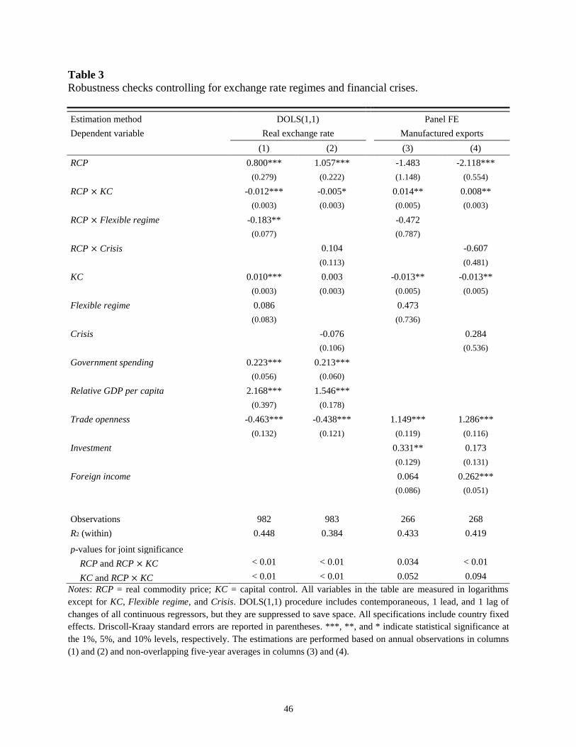
46

Table 3

Robustness checks controlling for exchange rate regimes and financial crises.

Estimation method DOLS(1,1) Panel FE

Dependent variable Real exchange rate Manufactured exports

(1) (2) (3) (4)

RCP 0.800*** 1.057*** -1.483 -2.118***

(0.279) (0.222) (1.148) (0.554)

RCP × KC -0.012*** -0.005* 0.014** 0.008**

(0.003) (0.003) (0.005) (0.003)

RCP × Flexible regime -0.183** -0.472

(0.077) (0.787)

RCP × Crisis 0.104 -0.607

(0.113) (0.481)

KC 0.010*** 0.003 -0.013** -0.013**

(0.003) (0.003) (0.005) (0.005)

Flexible regime 0.086 0.473

(0.083) (0.736)

Crisis -0.076 0.284

(0.106) (0.536)

Government spending 0.223*** 0.213***

(0.056) (0.060)

Relative GDP per capita 2.168*** 1.546***

(0.397) (0.178)

Trade openness -0.463*** -0.438*** 1.149*** 1.286***

(0.132) (0.121) (0.119) (0.116)

Investment 0.331** 0.173

(0.129) (0.131)

Foreign income 0.064 0.262***

(0.086) (0.051)

Observations 982 983 266 268

R2 (within) 0.448 0.384 0.433 0.419

p-values for joint significance

RCP and RCP × KC < 0.01 < 0.01 0.034 < 0.01

KC and RCP × KC < 0.01 < 0.01 0.052 0.094

Notes: RCP = real commodity price; KC = capital control. All variables in the table are measured in logarithms

except for KC, Flexible regime, and Crisis. DOLS(1,1) procedure includes contemporaneous, 1 lead, and 1 lag of

changes of all continuous regressors, but they are suppressed to save space. All specifications include country fixed

effects. Driscoll-Kraay standard errors are reported in parentheses. ***, **, and * indicate statistical significance at

the 1%, 5%, and 10% levels, respectively. The estimations are performed based on annual observations in columns

(1) and (2) and non-overlapping five-year averages in columns (3) and (4).

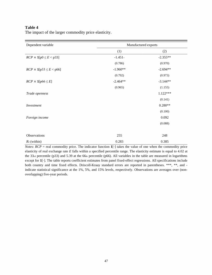
47

Table 4

The impact of the larger commodity price elasticity.

Dependent variable Manufactured exports

(1) (2)

RCP × 1[p0 ≤ E < p33] -1.451+ -2.355**

(0.786) (0.970)

RCP × 1[p33 ≤ E < p66] -1.960** -2.694**

(0.792) (0.973)

RCP × 1[p66 ≤ E] -2.464** -3.144**

(0.965) (1.155)

Trade openness 1.122***

(0.141)

Investment 0.280**

(0.100)

Foreign income 0.092

(0.088)

Observations 255 248

R2 (within) 0.283 0.385

Notes: RCP = real commodity price. The indicator function 1[·] takes the value of one when the commodity price

elasticity of real exchange rate E falls within a specified percentile range. The elasticity estimate is equal to 4.02 at

the 33rd percentile (p33) and 5.39 at the 66th percentile (p66). All variables in the table are measured in logarithms

except for 1[·]. The table reports coefficient estimates from panel fixed-effect regressions. All specifications include

both country and time fixed effects. Driscoll-Kraay standard errors are reported in parentheses. ***, **, and +

indicate statistical significance at the 1%, 5%, and 15% levels, respectively. Observations are averages over (non-

overlapping) five-year periods.

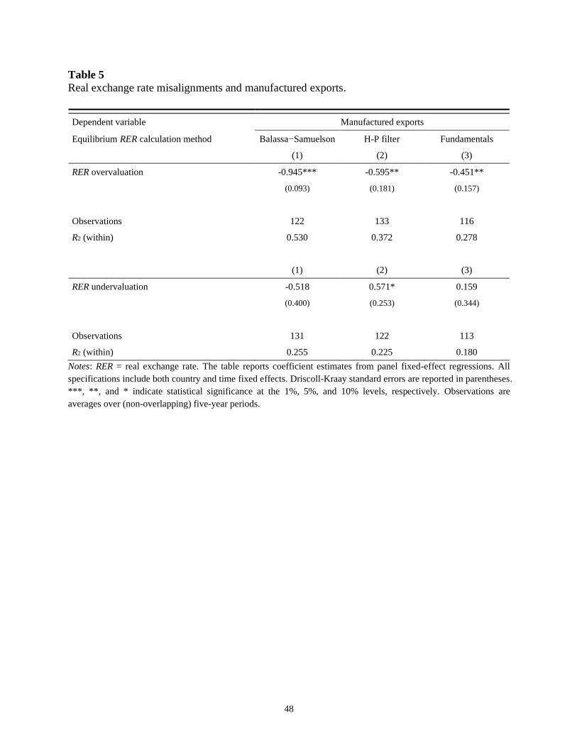
48

Table 5

Real exchange rate misalignments and manufactured exports.

Dependent variable Manufactured exports

Equilibrium RER calculation method Balassa−Samuelson H-P filter Fundamentals

(1) (2) (3)

RER overvaluation -0.945*** -0.595** -0.451**

(0.093) (0.181) (0.157)

Observations 122 133 116

R2 (within) 0.530 0.372 0.278

(1) (2) (3)

RER undervaluation -0.518 0.571* 0.159

(0.400) (0.253) (0.344)

Observations 131 122 113

R2 (within) 0.255 0.225 0.180

Notes: RER = real exchange rate. The table reports coefficient estimates from panel fixed-effect regressions. All

specifications include both country and time fixed effects. Driscoll-Kraay standard errors are reported in parentheses.

***, **, and * indicate statistical significance at the 1%, 5%, and 10% levels, respectively. Observations are

averages over (non-overlapping) five-year periods.

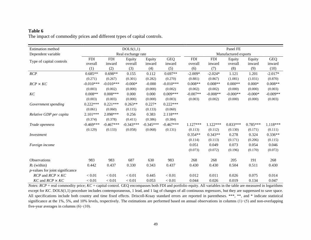
49

Table 6

The impact of commodity prices and different types of capital controls.

Estimation method DOLS(1,1) Panel FE

Dependent variable Real exchange rate Manufactured exports

Type of capital controls FDI

overall

FDI

inward

Equity

overall

Equity

inward

GEQ

inward

FDI

overall

FDI

inward

Equity

overall

Equity

inward

GEQ

inward

(1) (2) (3) (4) (5) (6) (7) (8) (9) (10)

RCP 0.685** 0.698** 0.155 0.112 0.697** -2.009* -2.024* 1.121 1.201 -2.017*

(0.271) (0.267) (0.301) (0.282) (0.270) (0.881) (0.867) (1.081) (1.031) (0.870)

RCP × KC -0.010*** -0.010*** -0.000* -0.000 -0.010*** 0.008** 0.008** 0.000** 0.000* 0.008**

(0.003) (0.002) (0.000) (0.000) (0.002) (0.002) (0.002) (0.000) (0.000) (0.003)

KC 0.008** 0.008*** 0.000 0.000 0.009*** -0.007** -0.008** -0.000** -0.000* -0.009**

(0.003) (0.003) (0.000) (0.000) (0.003) (0.003) (0.002) (0.000) (0.000) (0.003)

Government spending 0.222*** 0.221*** 0.263** 0.227* 0.222***

(0.061) (0.060) (0.115) (0.133) (0.060)

Relative GDP per capita 2.101*** 2.098*** 0.256 0.383 2.118***

(0.374) (0.378) (0.411) (0.386) (0.384)

Trade openness -0.469*** -0.467*** -0.343*** -0.345*** -0.467*** 1.127*** 1.122*** 0.833*** 0.785*** 1.118***

(0.129) (0.133) (0.058) (0.068) (0.131) (0.113) (0.112) (0.130) (0.171) (0.111)

Investment 0.354** 0.343** 0.278 0.324 0.336**

(0.114) (0.113) (0.171) (0.206) (0.115)

Foreign income 0.051 0.049 0.073 0.054 0.046

(0.073) (0.072) (0.196) (0.170) (0.072)

Observations 983 983 687 630 983 268 268 205 191 268

R2 (within) 0.442 0.437 0.330 0.343 0.437 0.430 0.430 0.504 0.511 0.430

p-values for joint significance

RCP and RCP × KC < 0.01 < 0.01 < 0.01 0.445 < 0.01 0.012 0.011 0.026 0.075 0.014

KC and RCP × KC < 0.01 < 0.01 < 0.01 0.053 < 0.01 0.044 0.026 0.019 0.134 0.047

Notes: RCP = real commodity price; KC = capital control. GEQ encompasses both FDI and portfolio equity. All variables in the table are measured in logarithms

except for KC. DOLS(1,1) procedure includes contemporaneous, 1 lead, and 1 lag of changes of all continuous regressors, but they are suppressed to save space.

All specifications include both country and time fixed effects. Driscoll-Kraay standard errors are reported in parentheses. ***, **, and * indicate statistical

significance at the 1%, 5%, and 10% levels, respectively. The estimations are performed based on annual observations in columns (1)−(5) and non-overlapping

five-year averages in columns (6)−(10).

50

Appendix A. List of sample countries and commodities

A.1. Sample countries

Our sample countries include: Argentina, Bangladesh, Bolivia, Brazil, Burundi, Central

African Republic, Chile, Costa Rica, Cote d’Ivoire, Ghana, Guatemala, Honduras, India, Kenya,

Madagascar, Malawi, Mali, Mauritania, Mauritius, Morocco, Mozambique, Niger, Pakistan,

Papua New Guinea, Paraguay, Peru, Philippines, Senegal, South Africa, Sri Lanka, Sudan,

Thailand, Togo, Turkey, Uganda, Uruguay, and Zambia.

A.2. Commodities used in the construction of commodity price indices

The list of 58 commodities includes: aluminum, bananas, barley, beef, coal, cocoa,

coconut oil, coffee, copper, copra, cotton, crude oil (petroleum), fish, fishmeal, gold, groundnuts

(peanuts), groundnut oil, hard logs, hardwood sawn, hides, iron ore, lamb, lead, maize, natural

gas, nickel, olive oil, oranges, palm kernel oil, palm oil, phosphate rock, potash, poultry

(chicken), rapeseed oil, rice, rubber, shrimp, silver, soft logs, softwood sawn, sorghum, soybean

meal, soybean oil, soybeans, sugar, sunflower oil, swine, tea, tin, tobacco, TSP (triple

superphosphate), uranium, urea, wheat, wood pulp, wool (coarse), wool (fine), and zinc.

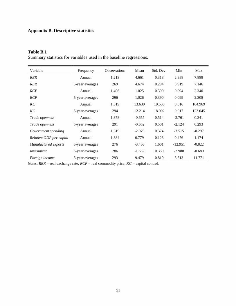
51

Appendix B. Descriptive statistics

Table B.1

Summary statistics for variables used in the baseline regressions.

Variable Frequency Observations Mean Std. Dev. Min Max

RER Annual 1,213 4.661 0.318 2.958 7.888

RER 5-year averages 269 4.674 0.294 3.919 7.146

RCP Annual 1,406 1.025 0.390 0.094 2.340

RCP 5-year averages 296 1.026 0.390 0.099 2.308

KC Annual 1,319 13.630 19.530 0.016 164.969

KC 5-year averages 294 12.214 18.002 0.017 123.045

Trade openness Annual 1,378 -0.655 0.514 -2.761 0.341

Trade openness 5-year averages 291 -0.652 0.501 -2.124 0.293

Government spending Annual 1,319 -2.079 0.374 -3.515 -0.297

Relative GDP per capita Annual 1,384 0.779 0.123 0.476 1.174

Manufactured exports 5-year averages 276 -3.466 1.601 -12.951 -0.822

Investment 5-year averages 286 -1.632 0.350 -2.980 -0.680

Foreign income 5-year averages 293 9.479 0.810 6.613 11.771

Notes: RER = real exchange rate; RCP = real commodity price; KC = capital control.

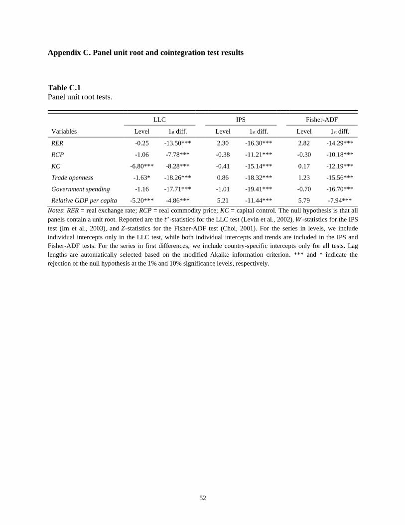
52

Appendix C. Panel unit root and cointegration test results

Table C.1

Panel unit root tests.

LLC IPS Fisher-ADF

Variables Level 1st diff. Level 1st diff. Level 1st diff.

RER -0.25 -13.50*** 2.30 -16.30*** 2.82 -14.29***

RCP -1.06 -7.78*** -0.38 -11.21*** -0.30 -10.18***

KC -6.80*** -8.28*** -0.41 -15.14*** 0.17 -12.19***

Trade openness -1.63* -18.26*** 0.86 -18.32*** 1.23 -15.56***

Government spending -1.16 -17.71*** -1.01 -19.41*** -0.70 -16.70***

Relative GDP per capita -5.20*** -4.86*** 5.21 -11.44*** 5.79 -7.94***

Notes: RER = real exchange rate; RCP = real commodity price; KC = capital control. The null hypothesis is that all

panels contain a unit root. Reported are the 𝑡∗-statistics for the LLC test (Levin et al., 2002), 𝑊-statistics for the IPS

test (Im et al., 2003), and 𝑍-statistics for the Fisher-ADF test (Choi, 2001). For the series in levels, we include

individual intercepts only in the LLC test, while both individual intercepts and trends are included in the IPS and

Fisher-ADF tests. For the series in first differences, we include country-specific intercepts only for all tests. Lag

lengths are automatically selected based on the modified Akaike information criterion. *** and * indicate the

rejection of the null hypothesis at the 1% and 10% significance levels, respectively.

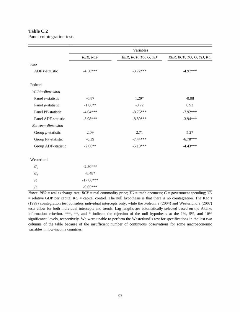
53

Table C.2

Panel cointegration tests.

Variables

RER, RCP RER, RCP, TO, G, YD RER, RCP, TO, G, YD, KC

Kao

ADF 𝑡-statistic -4.50*** -3.72*** -4.97***

Pedroni

Within-dimension

Panel 𝑣-statistic -0.87 1.29* -0.08

Panel 𝜌-statistic -1.86** -0.72 0.93

Panel PP-statistic -4.04*** -8.76*** -7.92***

Panel ADF-statistic -3.08*** -8.89*** -3.94***

Between-dimension

Group 𝜌-statistic 2.09 2.71 5.27

Group PP-statistic -0.39 -7.44*** -6.70***

Group ADF-statistic -2.06** -5.10*** -4.43***

Westerlund

𝐺𝑡 -2.30***

𝐺𝑎 -8.48*

𝑃𝑡 -17.06***

𝑃𝑎 -9.05***

Notes: RER = real exchange rate; RCP = real commodity price; TO = trade openness; G = government spending; YD

= relative GDP per capita; KC = capital control. The null hypothesis is that there is no cointegration. The Kao’s

(1999) cointegration test considers individual intercepts only, while the Pedroni’s (2004) and Westerlund’s (2007)

tests allow for both individual intercepts and trends. Lag lengths are automatically selected based on the Akaike

information criterion. ***, **, and * indicate the rejection of the null hypothesis at the 1%, 5%, and 10%

significance levels, respectively. We were unable to perform the Westerlund’s test for specifications in the last two

columns of the table because of the insufficient number of continuous observations for some macroeconomic

variables in low-income countries.

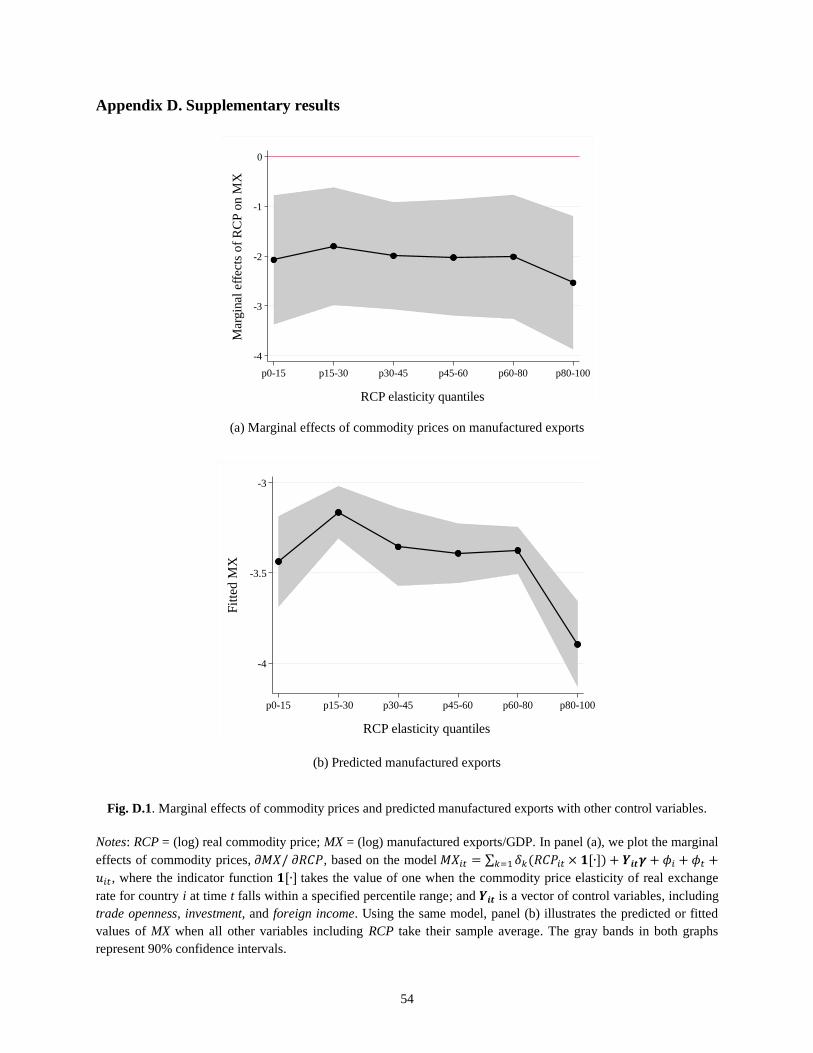
54

Appendix D. Supplementary results

(a) Marginal effects of commodity prices on manufactured exports

(b) Predicted manufactured exports

Fig. D.1. Marginal effects of commodity prices and predicted manufactured exports with other control variables.

Notes: RCP = (log) real commodity price; MX = (log) manufactured exports/GDP. In panel (a), we plot the marginal

effects of commodity prices, 𝜕𝑀𝑋/ 𝜕𝑅𝐶𝑃, based on the model 𝑀𝑋𝑖𝑡 = ∑ 𝛿𝑘(𝑅𝐶𝑃𝑖𝑡 × 𝟏[∙])𝑘=1 + 𝒀𝒊𝒕𝜸 + 𝜙𝑖 + 𝜙𝑡 +

𝑢𝑖𝑡, where the indicator function 𝟏[∙] takes the value of one when the commodity price elasticity of real exchange

rate for country i at time t falls within a specified percentile range; and 𝒀𝒊𝒕 is a vector of control variables, including

trade openness, investment, and foreign income. Using the same model, panel (b) illustrates the predicted or fitted

values of MX when all other variables including RCP take their sample average. The gray bands in both graphs

represent 90% confidence intervals.

-4

-3

-2

-1

0

Mar

gin

al e

ffec

ts o

f R

CP

on M

X

p0-15 p15-30 p30-45 p45-60 p60-80 p80-100

RCP elasticity quantiles

-4

-3.5

-3

Fit

ted M

X

p0-15 p15-30 p30-45 p45-60 p60-80 p80-100

RCP elasticity quantiles

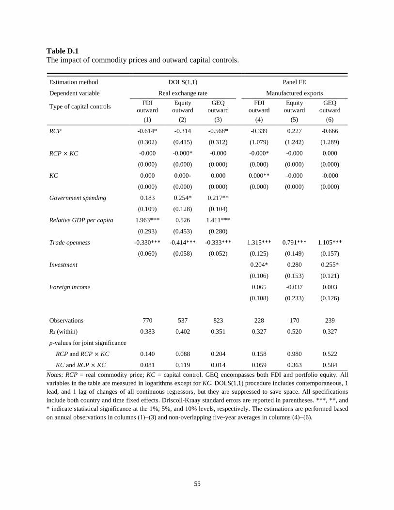
55

Table D.1

The impact of commodity prices and outward capital controls.

Estimation method DOLS(1,1) Panel FE

Dependent variable Real exchange rate Manufactured exports

Type of capital controls FDI

outward

Equity

outward

GEQ

outward

FDI

outward

Equity

outward

GEQ

outward

(1) (2) (3) (4) (5) (6)

RCP -0.614* -0.314 -0.568* -0.339 0.227 -0.666

(0.302) (0.415) (0.312) (1.079) (1.242) (1.289)

RCP × KC -0.000 -0.000* -0.000 -0.000* -0.000 0.000

(0.000) (0.000) (0.000) (0.000) (0.000) (0.000)

KC 0.000 0.000+ 0.000 0.000** -0.000 -0.000

(0.000) (0.000) (0.000) (0.000) (0.000) (0.000)

Government spending 0.183 0.254* 0.217**

(0.109) (0.128) (0.104)

Relative GDP per capita 1.963*** 0.526 1.411***

(0.293) (0.453) (0.280)

Trade openness -0.330*** -0.414*** -0.333*** 1.315*** 0.791*** 1.105***

(0.060) (0.058) (0.052) (0.125) (0.149) (0.157)

Investment 0.204* 0.280 0.255*

(0.106) (0.153) (0.121)

Foreign income 0.065 -0.037 0.003

(0.108) (0.233) (0.126)

Observations 770 537 823 228 170 239

R2 (within) 0.383 0.402 0.351 0.327 0.520 0.327

p-values for joint significance

RCP and RCP × KC 0.140 0.088 0.204 0.158 0.980 0.522

KC and RCP × KC 0.081 0.119 0.014 0.059 0.363 0.584

Notes: RCP = real commodity price; KC = capital control. GEQ encompasses both FDI and portfolio equity. All

variables in the table are measured in logarithms except for KC. DOLS(1,1) procedure includes contemporaneous, 1

lead, and 1 lag of changes of all continuous regressors, but they are suppressed to save space. All specifications

include both country and time fixed effects. Driscoll-Kraay standard errors are reported in parentheses. ***, **, and

* indicate statistical significance at the 1%, 5%, and 10% levels, respectively. The estimations are performed based

on annual observations in columns (1)−(3) and non-overlapping five-year averages in columns (4)−(6).

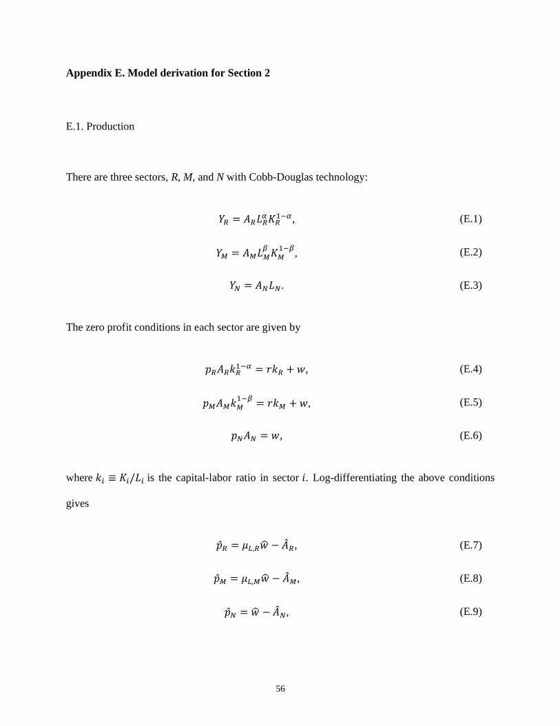
56

Appendix E. Model derivation for Section 2

E.1. Production

There are three sectors, R, M, and N with Cobb-Douglas technology:

𝑌𝑅 = 𝐴𝑅𝐿𝑅𝛼 𝐾𝑅

1−𝛼, (E.1)

𝑌𝑀 = 𝐴𝑀𝐿𝑀𝛽

𝐾𝑀1−𝛽

, (E.2)

𝑌𝑁 = 𝐴𝑁𝐿𝑁. (E.3)

The zero profit conditions in each sector are given by

𝑝𝑅𝐴𝑅𝑘𝑅1−𝛼 = 𝑟𝑘𝑅 + 𝑤, (E.4)

𝑝𝑀𝐴𝑀𝑘𝑀1−𝛽

= 𝑟𝑘𝑀 + 𝑤, (E.5)

𝑝𝑁𝐴𝑁 = 𝑤, (E.6)

where 𝑘𝑖 ≡ 𝐾𝑖/𝐿𝑖 is the capital-labor ratio in sector 𝑖. Log-differentiating the above conditions

gives

��𝑅 = 𝜇𝐿,𝑅�� − ��𝑅, (E.7)

��𝑀 = 𝜇𝐿,𝑀�� − ��𝑀, (E.8)

��𝑁 = �� − ��𝑁, (E.9)

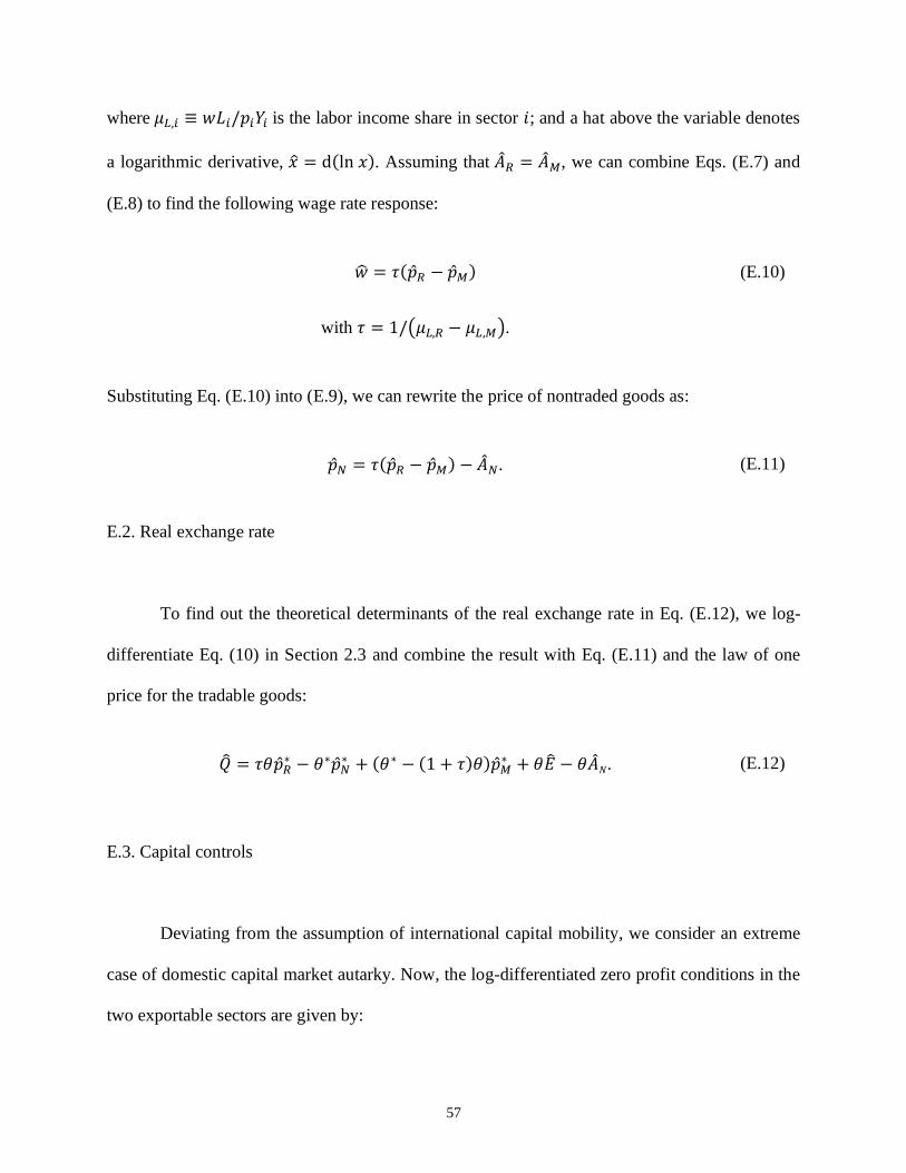
57

where 𝜇𝐿,𝑖 ≡ 𝑤𝐿𝑖/𝑝𝑖𝑌𝑖 is the labor income share in sector 𝑖; and a hat above the variable denotes

a logarithmic derivative, �� = d(ln 𝑥). Assuming that ��𝑅 = ��𝑀, we can combine Eqs. (E.7) and

(E.8) to find the following wage rate response:

�� = 𝜏(��𝑅 − ��𝑀) (E.10)

with 𝜏 = 1/(𝜇𝐿,𝑅 − 𝜇𝐿,𝑀).

Substituting Eq. (E.10) into (E.9), we can rewrite the price of nontraded goods as:

��𝑁 = 𝜏(��𝑅 − ��𝑀) − ��𝑁. (E.11)

E.2. Real exchange rate

To find out the theoretical determinants of the real exchange rate in Eq. (E.12), we log-

differentiate Eq. (10) in Section 2.3 and combine the result with Eq. (E.11) and the law of one

price for the tradable goods:

�� = 𝜏𝜃��𝑅∗ − 𝜃∗��𝑁

∗ + (𝜃∗ − (1 + 𝜏)𝜃)��𝑀∗ + 𝜃�� − 𝜃��𝑁. (E.12)

E.3. Capital controls

Deviating from the assumption of international capital mobility, we consider an extreme

case of domestic capital market autarky. Now, the log-differentiated zero profit conditions in the

two exportable sectors are given by:

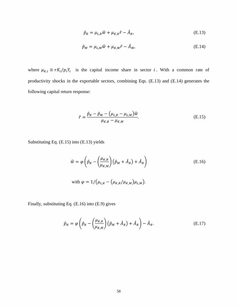
58

��𝑅 = 𝜇𝐿,𝑅�� + 𝜇𝐾,𝑅 �� − ��𝑅, (E.13)

��𝑀 = 𝜇𝐿,𝑀�� + 𝜇𝐾,𝑀�� − ��𝑀, (E.14)

where 𝜇𝐾,𝑖 ≡ 𝑟𝐾𝑖/𝑝𝑖𝑌𝑖 is the capital income share in sector 𝑖 . With a common rate of

productivity shocks in the exportable sectors, combining Eqs. (E.13) and (E.14) generates the

following capital return response:

�� =��𝑅 − ��𝑀 − (𝜇𝐿,𝑅 − 𝜇𝐿,𝑀)��

𝜇𝐾,𝑅 − 𝜇𝐾,𝑀. (E.15)

Substituting Eq. (E.15) into (E.13) yields

�� = 𝜑 (��𝑅 − (𝜇𝐾,𝑅

𝜇𝐾,𝑀) (��𝑀 + ��𝑅) + ��𝑅) (E.16)

with 𝜑 = 1/(𝜇𝐿,𝑅 − (𝜇𝐾,𝑅/𝜇𝐾,𝑀)𝜇𝐿,𝑀).

Finally, substituting Eq. (E.16) into (E.9) gives

��𝑁 = 𝜑 (��𝑅 − (𝜇𝐾,𝑅

𝜇𝐾,𝑀) (��𝑀 + ��𝑅) + ��𝑅) − ��𝑁 . (E.17)