Color Measurement Using a Smartphone Applied to Madeira Wines · Color Measurement Using a...
100
January | 2015 PM José Carlos Vieira da Silva MASTER IN INFORMATICS ENGINEERING Color Measurement Using a Smartphone Applied to Madeira Wines MASTER PROJECT
Transcript of Color Measurement Using a Smartphone Applied to Madeira Wines · Color Measurement Using a...

January | 2015
PM
José Carlos Vieira da SilvaMASTER IN INFORMATICS ENGINEERING
Color Measurement Usinga Smartphone Appliedto Madeira WinesMASTER PROJECT

CO-SUPERVISORMon-Chu Chen
SUPERVISORJosé Carlos Marques
José Carlos Vieira da SilvaMASTER IN INFORMATICS ENGINEERING
Color Measurement Usinga Smartphone Appliedto Madeira WinesMASTER PROJECT

Color Measurement Using a Smartphone Applied to Madeira Wines
José Carlos Vieira da Silva
Jury composition:
, Professor Karolina Baras
, Professor José Carlos Marques
, Professor Yoram Chisik
March 2015
Funchal – Portugal

i
RESUMO
A visão computacional é uma área que usa técnicas para adquirir, processar, analisar
e perceber imagens do mundo real de modo a produzir informação numérica ou simbólica na
forma de decisões [1].
Este projeto tem como objetivo utilizar a visão computacional para analisar uma
amostra de vinho Madeira e caraterizá-la pela sua cor (vinhos doces ou secos, novos ou
envelhecidos têm uma cor específica).
Utiliza-se técnicas de comparação de histogramas para analisar as imagens captadas
de uma amostra num recipiente especial criado para este propósito.
A análise da cor de uma amostra de vinho através de uma imagem obtida a partir de
um smartphone pode ser difícil. A imagem captada pode ser influenciada por vários fatores
tais como, a iluminação, o que está por trás da amostra (fundo da imagem) devido às várias
posições em que a imagem pode ser obtida (diferente captar a imagem contra uma parede ou
contra o chão).
Através do uso de novas tecnologias como a impressão 3D, foi possível criar um
protótipo que visa controlar o efeito de fatores ambientais externos na imagem captada.
Os resultados alcançados deixam bons indícios para futuros trabalhos. Apesar de ser
necessário efetuar mais testes, os primeiros realizados tiveram uma taxa de sucesso na
ordem dos 80% a 90% de resultados corretos.
Este relatório documenta o desenvolvimento deste projeto e todas as técnicas e
passos necessários para executar os testes.


iii
PALAVRAS-CHAVE
Visão-computacional
Vinho Madeira
Cor
Smartphone
Impressão 3D
Histogramas

v
ABSTRACT
Computer vision is a field that uses techniques to acquire, process, analyze and
understand images from the real world in order to produce numeric or symbolic information in
the form of decisions [1].
This project aims to use computer vision to prepare an app to analyze a Madeira Wine
and characterize it (identify its variety) by its color. Dry or sweet wines, young or old wines
have a specific color.
It uses techniques to compare histograms in order to analyze the images taken from a
test sample inside a special container designed for this purpose.
The color analysis from a wine sample using an image captured by a smartphone can
be difficult. Many factors affect the captured image such as, light conditions, the background
of the sample container due to the many positions the photo can be taken (different to capture
facing a white wall or facing the floor for example).
Using new technologies such as 3D printing it was possible to create a prototype that
aims to control the effect of those external factors on the captured image.
The results for this experiment are good indicators for future works. Although it’s
necessary to do more tests, the first tests had a success rate of 80% to 90% of correct results.
This report documents the development of this project and all the techniques and steps
required to execute the tests.

vii
KEYWORDS
Computer-vision
Madeira Wine
Color
Smartphone
3D Printing
Histograms


ix
ACKNOWLEDGEMENTS
I want to thank all of those that somehow influenced me or helped me through the
development of this project.
Professor José Carlos Marques and Professor Mon-Chu Chen for all the orientation on
this project.
To all my colleagues that always helped me when I needed most. Special thanks for
all the chemistry colleagues that helped me with the wines and all the tests on the lab.
To Madeira Wine Company for all the samples provided under the IMPACT II project.
To my family, especially my parents that always supported me since the beginning of
my studies.
A special thanks to Marisa for always encouraging me to do this project and for being
always by my side and for keeping pushing me forward.


xi
INDEX
1 Introduction ........................................................................................................ 1
1.1 Motivation .................................................................................................................... 2
1.2 Goals ............................................................................................................................ 2
1.3 Document Organization ............................................................................................. 2
2 State of the art .................................................................................................... 5
2.1 Color measurement .................................................................................................... 5
2.2 Wine color measurement ........................................................................................... 6
2.2.1 Related work........................................................................................................................ 7
3 Domain research ................................................................................................ 9
3.1 Madeira wine ............................................................................................................... 9
3.1.1 Madeira Wine color .............................................................................................................. 9
3.2 Digital cameras ......................................................................................................... 10
3.2.1 Components and Technical Details ................................................................................... 10
3.2.1.1 Sensor ........................................................................................................................... 10
3.2.1.2 Camera Resolution ....................................................................................................... 11
3.2.1.3 Capturing Color ............................................................................................................. 11
3.2.1.4 Exposure and Focus ..................................................................................................... 12
3.2.1.5 Lenses .......................................................................................................................... 13
3.2.1.6 Storing Digital Photos .................................................................................................... 13
3.2.2 Smartphone cameras ........................................................................................................ 13
3.3 Color ........................................................................................................................... 14
3.3.1 Human Color Perception ................................................................................................... 14
3.3.2 Representing Color ............................................................................................................ 16
3.3.2.1 Color models/spaces ..................................................................................................... 16
3.3.2.1.1 RGB........................................................................................................................ 16
3.3.2.1.2 L*a*b* ..................................................................................................................... 17
3.3.2.1.3 HSV ........................................................................................................................ 17
3.4 3D Printing ................................................................................................................. 18
3.4.1 Impact of 3D printing in industry ........................................................................................ 19
3.5 iOS Development ...................................................................................................... 21
3.6 Histogram .................................................................................................................. 23
4 Implementation ................................................................................................ 25
4.1 Initial approach ......................................................................................................... 25
4.1.1 Lessons learned ................................................................................................................ 27

xii
4.2 3D prototypes............................................................................................................ 27
4.2.1 Blackbox ............................................................................................................................ 28
4.2.1.1 Blackbox assembly ....................................................................................................... 30
4.2.2 Recipient Cover ................................................................................................................. 33
4.2.3 Lessons learned ................................................................................................................ 34
4.3 System Architecture................................................................................................. 36
4.3.1 System Requirements ....................................................................................................... 36
4.3.1.1 Functional requirements ................................................................................................ 36
4.3.1.2 Non-functional requirements ......................................................................................... 36
4.3.2 Use Case Diagram ............................................................................................................ 37
4.3.3 Class Diagram ................................................................................................................... 38
4.3.4 Interface prototypes ........................................................................................................... 39
4.3.4.1 Main Screen .................................................................................................................. 40
4.3.4.2 Varieties Screen ............................................................................................................ 41
4.3.4.3 Base Samples Screen ................................................................................................... 42
4.3.4.4 New Base Sample Screens........................................................................................... 43
4.3.4.5 New Test Screen ........................................................................................................... 45
4.3.4.6 Results Screen .............................................................................................................. 45
4.3.5 Final Interface and evolution.............................................................................................. 46
4.3.6 Lessons learned ................................................................................................................ 49
4.4 Software ..................................................................................................................... 49
4.4.1 Version 1 ........................................................................................................................... 49
4.4.2 Version 2 ........................................................................................................................... 52
4.4.3 Version 3 ........................................................................................................................... 54
4.4.4 Version 4 ........................................................................................................................... 56
4.4.5 Final improvements ........................................................................................................... 57
4.5 Logo ........................................................................................................................... 58
4.6 Splash screen ........................................................................................................... 58
5 Tests and results ............................................................................................. 59
5.1 Procedure .................................................................................................................. 59
5.1.1 Step 1 ................................................................................................................................ 60
5.1.2 Step 2 ................................................................................................................................ 61
5.1.3 Step 3 ................................................................................................................................ 62
5.2 Results Analysis ....................................................................................................... 63
6 Conclusions ..................................................................................................... 67
7 Future work ...................................................................................................... 69
8 References ....................................................................................................... 71
9 Appendix .......................................................................................................... 74

xiii
9.1 Appendix 1 – Image size tests ................................................................................ 74
9.2 Appendix 2 – Image comparison flowchart ........................................................... 76
9.3 Appendix 3 – How the Eye Sees in Color [19] ....................................................... 77


xv
FIGURE LIST
Figure 2.1 - Color picker example .............................................................................................. 5
Figure 2.2 - ColorMeter - iOS App [3] ........................................................................................ 6
Figure 2.3 - Shimadzu UV-2600 UV-VIS spectrophotometer [6] ............................................... 7
Figure 3.1 - Madeira Wine color variations [8] ........................................................................... 9
Figure 3.2- CCD sensor [9] ...................................................................................................... 10
Figure 3.3 - Bayer Sensor interpolation [10] ............................................................................ 11
Figure 3.4 - Bayer filter pattern [11] ......................................................................................... 12
Figure 3.5 - RAW image [12] .................................................................................................... 12
Figure 3.6 - Smartphone camera sensors [14] ........................................................................ 14
Figure 3.7 - How the human eye sees color [19] ..................................................................... 15
Figure 3.8 - RGB cube representation [21] .............................................................................. 17
Figure 3.9 - CIELAB coordinate system [22] ........................................................................... 17
Figure 3.10 - HSV Color model mapped to a cylinder [24] ...................................................... 18
Figure 3.11 - Google SketchUp overview ................................................................................ 19
Figure 3.12 - Ultimaker Original 3D Printer .............................................................................. 19
Figure 3.13 - 3D printing in industry [28] .................................................................................. 20
Figure 3.14 - 3D laser printing [30]........................................................................................... 20
Figure 3.15 - CNC machining waste material [31] ................................................................... 21
Figure 3.16- iOS Development overview [33] .......................................................................... 22
Figure 3.17 - XCode Overview [34] .......................................................................................... 23
Figure 3.18 - Histogram example [36] ...................................................................................... 23
Figure 4.1 - Red rule and pallet ................................................................................................ 25
Figure 4.2 - Red rule and pallet, different angle ...................................................................... 25
Figure 4.3 - Paper prototype .................................................................................................... 28
Figure 4.4 - Captured image without controlling flash light ..................................................... 28
Figure 4.5 - First 3D Blackbox prototype ................................................................................. 29
Figure 4.6 - Blackbox 3D model ............................................................................................... 29
Figure 4.7 - 3D printer producing the Blackbox ....................................................................... 30
Figure 4.8 - Blackbox pieces as printed ................................................................................... 31
Figure 4.9 - Drawing the Blackbox faces on paper .................................................................. 31
Figure 4.10 - Interior padding ................................................................................................... 32
Figure 4.11 - Blackbox, final build ............................................................................................ 33
Figure 4.12 - Quartz recipient and original cover..................................................................... 33
Figure 4.13 - Quartz recipient and cork ................................................................................... 34
Figure 4.14 - Soft plastic cover ................................................................................................ 34
Figure 4.15 - 3D model for soft plastic cover ........................................................................... 34
Figure 4.16 - Use Case Diagram ............................................................................................. 37
Figure 4.17 - Class Diagram .................................................................................................... 38
Figure 4.18 - Main screen prototype ........................................................................................ 40

xvi
Figure 4.19 - Main screen, settings menu prototype ............................................................... 40
Figure 4.20 - Varieties screen prototype .................................................................................. 41
Figure 4.21 - New variety screen prototype ............................................................................. 41
Figure 4.22 - Base samples screen prototype ........................................................................ 42
Figure 4.23 - Base samples screen prototype, delete sample ................................................ 42
Figure 4.24 - New base sample, screen prototype .................................................................. 43
Figure 4.25 - New base sample, use photo screen prototype ................................................. 43
Figure 4.26 - New base sample, select variety screen prototype ........................................... 44
Figure 4.27 - Name new base sample, screen prototype ........................................................ 44
Figure 4.28 - Results screen prototype .................................................................................... 45
Figure 4.29 - Blackbox covering top buttons ........................................................................... 46
Figure 4.30 - Home Screen, final version ................................................................................ 47
Figure 4.31 - Home screen, Settings final version ................................................................... 47
Figure 4.32 - Varieties Screen, Final version ........................................................................... 48
Figure 4.33 - Base samples Screen, final version ................................................................... 48
Figure 4.34 - Captured image with controlled flash light ......................................................... 50
Figure 4.35 - Image comparison, with flash (left image) and without flash light (right image) 51
Figure 4.36 - Processing feedback .......................................................................................... 56
Figure 4.37 - App logo .............................................................................................................. 58
Figure 4.38 - App splash screen .............................................................................................. 58
Figure 5.1 - Preparing a sample to test .................................................................................... 60
Figure 5.2 - Inserting the test cell in the Blackbox prototype ................................................... 61
Figure 5.3 - Testing a sample................................................................................................... 62
Figure 5.4- Test results (Example) ........................................................................................... 63

xvii
TABLE LIST
Table 3.1 - The visible light spectrum ...................................................................................... 15
Table 4.1 - RGB and HSL values for rule in Figure 4.1 and Figure 4.2 .................................. 26
Table 4.2 - RGB and HSL values for color pallet in Figure 4.1 and Figure 4.2 ....................... 26
Table 4.3 - Comparison between object and palette lines in Figure 4.1 and Figure 4.2 ........ 26
Table 4.4 - Test inside home, normal light conditions ............................................................. 51
Table 4.5 - Test inside home, artificial light conditions ............................................................ 52
Table 4.6 - Test inside home, dark environment ..................................................................... 52
Table 4.7 - Image Size vs Test Time ....................................................................................... 57
Table 5.1 - Test results ............................................................................................................. 64


xix
ACRONYMS
3D – Three-Dimensional
CCD - complementary coupled device
CNC – Computer Numerical Control
HSL - Hue, Saturation, Luminance Color Model
HSV – Hue, Saturation, Value Color Model
iOS – iPhone Operating System
JPEG - Joint Photographic Experts Group
LAB (CIElab) – A color space defined by the Commission Internationale de l'Eclairage
LCD – Liquid Crystal Display
OS X - Macintosh Operating System X
RGB – Red, Green, Blue Color Model
SDK – Software Development Kit


1
1 INTRODUCTION
Smartphones are really popular nowadays. Their extraordinary processing power is
increasing continuously making them a powerful tool for many purposes other than just make
calls.
Engineers developed some ingenious applications and we can simply grab our
smartphones out from our pockets and analyze if a mole is cancerous or not, or we can
measure our heart rate. All of this is made using the camera on our smartphones together with
some computational algorithms.
Expensive machines can be replaced by these much cheaper devices that we can take
everywhere. Although, in some cases smartphones need to evolve more to be more accurate,
and it will be difficult to someone to trust a smartphone instead of a machine worth thousands
of euros.
Android and iOS are the most used systems in the smartphones world. Both have their
pros and cons but iOS is known by is stability and quality.
Currently Madeira Wine is being measured / characterized by its color at the University
of Madeira through the project IMPACT II (MADFDR-01-190-FEDR-000010) financed through
the Regional Development Institute, under the program ‘+ Conhecimento (INTERVIR +)’. Dry
or sweet wines, young or old have a specific color. This work is being done by Professor José
Carlos Marques from the Chemistry Department at the University of Madeira and is the base
for this project.
We can notice the sweetness and distinguish the wines using our senses. When we
smell or taste, we can tell if a glass of wine compared to another one is sweeter or not because
we can feel the sugar contained in the wine. Also, only looking at a glass of wine, by the color
we can tell the sweetness as dry wines are lighter than sweet wines.
Using the senses to identify something is tricky because the human beings don’t have
all the senses developed in the same way, also, it may require some practice and previous
knowledge related to Madeira Wine.
Although on the lab we can distinguish the wines, this option is not available to general
public, and even to professionals it requires some time to analyze the retrieved data.
There were 102 billion app downloads in 2013 with perspective to grow. It’s a high
profitable market, with billions in revenues. Specifically related to lab use of smartphones, the

2
number of app downloads to be used on the lab is not known, but it’s expectable to be a
sizeable portion. It has potential to grow [1].
The choice of a smartphone app to perform advanced experiments may be useful, as
almost everyone has a smartphone nowadays.
1.1 Motivation
Being able to reproduce the functions of an expensive laboratory machine in a
smartphone is a difficult challenge with lots of limitations but is also a great opportunity to
develop something new.
This can bring the opportunity for the wineries to test their wines to see if it fits within
the standards expected for that wine.
Madeira Wine is known worldwide. Associate new technologies to this product can
open doors to new opportunities, new markets.
Typical Madeira Wine consumers are older adult people, something like this project
can cause curiosity in other persons to buy the wine if a more commercial version of the app
reaches the regular consumer.
The idea of grabbing the smartphone, take a picture and get the variety of the wine can
lead to some changes in the fermentation process and in the quality control procedures.
1.2 Goals
This project intends to:
Prepare an app for a smartphone to identify a Madeira wine by the color.
1.3 Document Organization
This document is divided in seven main chapters.
The first chapter is the introduction were a brief description of the problem and the goal
of the project are stated.

3
The second chapter, the State of Art, describes how the problem is currently solved.
Some related works are also stated on this chapter.
On the third chapter, there is a domain research that includes all the relevant data for
this project. There are some notions about Madeira Wine, digital cameras, smartphone
cameras, color, 3D printing, developing for iOS and the notion of Histogram.
The fourth chapter is the implementation of the project. It describes all the steps and
procedures, how the idea was generated and evolved during the execution of the project. It
has also all the details about how the software was created and how it works. Contains also
the origin of the ideas for the App logo and splash screen.
On the fifth chapter, there is the description of the test procedure, the test results and
their analysis.
Chapter 6 is the conclusions for this project and report and an overall overview of the
work that was done.
Chapter 7 presents some ideas for future work. They can be implemented if the app is
intended to be published.


5
2 STATE OF THE ART
Although there is no related work (known to date) regarding the use of smartphones to
specifically measure wine color, they can be used to measure color from anything in a photo
using one of the many apps available built for this purpose.
Specifically related to wine color, there are some works that used other platforms to do
that function.
2.1 Color measurement
There are many mobile and desktop applications to measure color. Most of them work
the same way, the user clicks on some point of the test image and the software calculates and
displays the result using RGB, HSV, LAB, or other color models.
The following example in Figure 2.1, demonstrates the use of Adobe Photoshop to pick
the color values using different color representations from a clicked point.
Figure 2.1 - Color picker example
For mobile platforms, there are many more applications to measure color than there is
for other devices such as laptops. This market is growing as more and more smartphones are
reaching the market. For example, iOS app ColorMeter in Figure 2.2 displays the color of some
given point in an image in many color models such as RGB, HSV, Lab*, etc. [3].

6
Figure 2.2 - ColorMeter - iOS App [3]
2.2 Wine color measurement
Wine color measurement is a specific area where color measurement techniques are
applied.
Some work has been made in this area to predict the color of wine from grapes [4], to
ensure quality control [5] and in University of Madeira with the Madeira Wine color
characterization for example.
Wine color is very important for the perception of quality and is a useful indicator for
issues related to wine development and fermentation.
It’s important to keep color variations controlled. People expect some kind of wine to
be from a certain color. If the color variation is big, the consumers will be sceptic about that
wine.

7
Color monitoring is also useful to document the effect of fermentation variables on wine
color [5]. For example, when the new fermentation techniques are tested.
2.2.1 RELATED WORK
This work of establishing color standards and improve wine fermentation techniques
analyzing the color, applied to Madeira Wines, is being made at University of Madeira.
Two different techniques are used to try to define a color for each wine brand using
Ultraviolet–visible spectroscopy using the Glories method (measuring the absorbance at 420
nm, 520 nm and 620 nm) or by the CIElab method (using full Ultraviolet-visible spectrum).
The equipment used in this process, Shimadzu, model spectrophotometer UV-vis 2600
presented in Figure 2.3 is an expensive and complex machine.
This methods require practice and specific formation and competences because the
retrieved data is complex, so, only experienced technicians are able to perform those tests.
Figure 2.3 - Shimadzu UV-2600 UV-VIS spectrophotometer [6]


9
3 DOMAIN RESEARCH
This chapter covers some concepts that are highly important to understand this project.
Madeira Wine, digital cameras, smartphone cameras, color, 3D printing, developing for iOS
and the notion of Histogram are essential topics.
3.1 Madeira wine
Madeira Wine is a fortified wine produced in Madeira Island, Portugal.
This wine is available in different sweet/dry variations [7]. The grapes varietals define
the wine:
• Sercial – A white wine grape that is used to produce a dry style of Madeira.
• Verdelho – A white wine grape used to make a semi-dry variation of Madeira.
• Bual - A white grape that makes a semi-sweet Madeira.
• Malmsey – A white grape that typically registers sweet when made into Madeira.
Another varietal is Tinta Negra, a red grape which is the most common in the island.
This one has the particularity of being able to produce sweet, medium-sweet, dry and medium-
dry wines according how the producers conduct the fermentation process.
3.1.1 MADEIRA WINE COLOR
The different variations of Madeira have different characteristic colors.
Dry wines have a light yellow color, medium-dry a golden color, medium-sweet a dark
gold to brown color and finally sweet wine have a brown color has noticed in Figure 3.1.
Figure 3.1 - Madeira Wine color variations [8]

10
3.2 Digital cameras
Digital cameras work like a conventional camera. It has a series of lenses that focus
light to create an image of a scene. The difference is that instead of focusing the light onto a
piece of film, it focuses onto a semiconductor device that records light electronically. The
computer then breaks the electronic information to digital data.
3.2.1 COMPONENTS AND TECHNICAL DETAILS
This section covers some of the most important components and technical details
about digital cameras.
3.2.1.1 Sensor
The image sensor as the one presented in Figure 3.2 is used by most cameras and is
named Complementary Coupled Device (CCD). Its function is to convert light into electrons.
Simplifying, these sensors are a 2D array of thousands or millions of tiny cells.
Figure 3.2- CCD sensor [9]
Once the sensor converts the light into electrons, it reads the accumulated charge of
each cell in the image.
The CCD transports the charge across the chip and reads it at one corner of the array.
An analog-to-digital converter turns each pixel’s value into digital value by measuring the
amount of charge at each cell and converting that measurement to binary form.

11
3.2.1.2 Camera Resolution
The resolution is the amount of detail that the camera can capture and it’s measured
in pixels. The more pixels it has, the more detail can capture, and, consequently, the larger the
pictures can be without becoming blurry.
Resolution can vary from 256x256 to 4064x2704. Professional cameras can capture
over 16 million pixels or 20 million pixels for large-format cameras.
Common cameras usually have a minimum resolution of 640x480. It’s an ideal size for
e-mailing pictures or posting to a website.
3.2.1.3 Capturing Color
The sensor cells are colorblind, only keep track of the total intensity of the light that
strikes their surface. Most sensors use filtering to look at light in its three primary colors. Once
the three colors are captured, they are combined to create the full spectrum.
Highest quality cameras use three sensors, each with a different filter. The light is
directed to the different sensors that respond only to one of the primary colors. The advantage
is that the camera records each of the three colors at each pixel location but it’s an expensive
solution.
A more economical solution to record the primary colors is to place a permanent filter
called color filter array over each individual sensor cell.
By breaking up the sensor into a variety of red, green and blue pixels, using
interpolation, that means, look at the other pixels in the neighborhood of a sensor and make a
guess about the color at that central location it’s possible to get the color for all pixels. Figure
3.3 demonstrates the interpolation, which neighbor pixels are used to calculate the color.
Figure 3.3 - Bayer Sensor interpolation [10]

12
The most common pattern of filters is Bayer filter pattern. It alternates a row of red and
green filters with a row of blue and green filter. As seen in Figure 3.4, there are as many green
pixels as there are blue and red combined. This is due to the higher sensitivity the human eye
has to green color.
Figure 3.4 - Bayer filter pattern [11]
The advantages of this method are that only requires one sensor and all the color
information (red, green and blue) is recorded at the same moment. This means smaller
equipment’s and less costs.
Digital cameras use demosaicing algorithms to convert a mosaic into an equally sized
mosaic of true colors as the one in Figure 3.5.
Figure 3.5 - RAW image [12]
Each colored pixel can be used more than once, its true color can be determined by
averaging the values from the closest surrounding pixels.
3.2.1.4 Exposure and Focus
All cameras, digital or not, have to control the amount of light that reaches the sensor.
The two key elements used for this are the aperture and shutter speed.
13
Aperture: The size of the opening in the camera. It’s an automatic procedure in most
digital cameras, but, some allow manual adjustment to give professionals more control
over the final image.
Shutter speed: The amount of time that light can pass through the aperture.
These two elements work together to capture the amount of light needed to make a
good image. In photographic terms, they set the exposure of the sensor.
3.2.1.5 Lenses
Digital cameras have one of four types of lenses:
Fixed-focus, fixed-zoom lenses: Used on disposable cameras and
inexpensive film cameras.
Optical-zoom lenses with automatic focus: Similar to the video
camcorder lens. Has automatic focus, but it may not have manual focus.
They change the focal length of the lens rather than just magnifying the
information that hits the sensor.
Digital Zoom: The camera takes the central pixels from sensor and
interpolates them to make a full-sized image.
Replaceable lens system: These are similar to the replaceable lenses on
a 35mm camera. Some digital cameras can use 35mm camera lenses.
3.2.1.6 Storing Digital Photos
Most digital cameras have LCD screens that allow to see the picture immediately.
Storing images requires a lot of memory. Most cameras use JPEG file format for storing
pictures allowing to choose quality settings, for example, medium or high quality.
To make the most of their storage space, most digital cameras use data compression
to make the files smaller [13].
3.2.2 SMARTPHONE CAMERAS
Today’s smartphone cameras evolved a lot. Some of them are even more powerful
than some regular cameras, with better quality, more custom settings, etc.

14
All of them work with the same basis, a sensor and a lens. This hardware is basically
the same found on regular digital cameras, but they have the particularity of being really small
as shown in Figure 3.6 [14].
Figure 3.6 - Smartphone camera sensors [14]
The process to capture an image is the same. The light enters the camera via the lens
onto the sensor. There, in the sensor, sensible areas record light electronically and then the
computers converts this information to digital data [13].
These cameras, similarly to digital cameras, usually capture color using RGB that is a
color model that uses the three primary colors (red, green, blue) that is also the color model
used in displays [15].
3.3 Color
Color is a rich and complex experience, is the vision system responding differently to
different wavelengths of light [1].
3.3.1 HUMAN COLOR PERCEPTION
To describe colors is necessary to know how people respond to them. Human
perception of color is a complex context of: illumination, memory, object identity and emotion.
All of these aspects can influence the perception of color [1].
When light hits an object, some of it is absorbed and the remaining is reflected. The
wavelengths that are absorbed and reflected depend on the object. The reflected ones,
determine what color we see [16].

15
The visible spectrum is a portion of the electromagnetic spectrum that can be detected
by the human eye, typically called visible light. A typical human eye responds to wavelengths
from about 400-700nm [17]. Table 3.1 relates the color names to their wavelengths.
Table 3.1 - The visible light spectrum
COLOR WAVELENGTH (NM)
RED 625-740
ORANGE 590-625
YELLOW 565-590
GREEN 520-565
CYAN 500-520
BLUE 435-500
VIOLET 380-435
The following graphic in Figure 3.7 is a good resume for how the human eye works for
the reflected wavelengths.
A higher resolution image for better reading can be consulted in Appendix 3 – How the
Eye Sees in Color.
Figure 3.7 - How the human eye sees color [18]

16
This example can be applied for any object of any color.
Very concisely, the light waves hit the light-sensitive retina at the back of our eye. Then
the cones that are one type of photoreceptor, tiny cells in the retina that respond to light, are
stimulated. The resulting signal is transmitted through the optic nerve to the visual cortex of
the brain, which processes the information returning the perceived color.
Humans have three different cone types, which allows them to discern color better than
most mammals, but, plenty of animals have better vision capabilities.
Many fish and birds have four type of cones, enabling them to see ultraviolet light than
the human eye cannot perceive.
3.3.2 REPRESENTING COLOR
Color can be represented in many forms. A standard system is required to talk about
color. Simple names are insufficient because people can associate a large variety of colors
with a given name.
3.3.2.1 Color models/spaces
There is a large variety of color models or spaces, which means, how we can represent
a color in some scale. Some examples more relevant to this work are RGB, CIELAB and HSV
and are presented in this document.
3.3.2.1.1 RGB
RGB is a color model that uses the three primary colors (Red, Green and Blue) that
can be mixed to make all the other color. It is widely used throughout computer graphics and
it’s common to find a large amount of existing software routines since it’s been used for many
years [19].
This color model can be represented in form of a cube as shown in Figure 3.8.

17
Figure 3.8 - RGB cube representation [20]
3.3.2.1.2 L*a*b*
L*a*b* is one of the color space representations used in the Chemistry lab to represent
wine colors. L* represents the difference between light (L*=100) and dark (L*=0). A* represents
the difference between green (-a*) and red (+a*), and b* represents the difference between
yellow (+b*) and blue (-b*). Figure 3.9 represents the CIELAB coordinate system.
Figure 3.9 - CIELAB coordinate system [21]
This color model can be useful to manipulate images, as the luminance is separate
from the color information, however it’s not very simple to use because it’s not intuitive for most
people [21].
3.3.2.1.3 HSV
HSV stands for Hue, Saturation and Value. Hue is expressed in a number from 0 to
360 degrees. Red starts at 0, Yellow at 60, Green at 120, Cyan at 180, Blue at 240 and
Magenta starts at 300. Saturation is the amount of Grey (0% to 100%) in the color and Value
(or Brightness) works in conjunction with saturation and describes the brightness from 0% to
100% [22].

18
HSV can be represented as a cylinder as shown in Figure 3.10.
Figure 3.10 - HSV Color model mapped to a cylinder [23]
Different software use different scales, so, for this particular case, the OpenCV library
used to calculate and compare histograms on the app has a range of 0 to 179 for Hue and 0
to 255 for Saturation and Value [24].
3.4 3D Printing
3D Printing may sound like something new, something that appeared in the last two or
three years. Actually, this notion appeared around 1980 when Chuck Hull created technology
to print 3D objects from digital data [25].
The Boom of 3D Printing occurred recently, around two or three years ago as many
brands released their domestic 3D printers to the market. With prices around 2000€ for the
cheapest printers, it’s not a technology available to everyone. Another problem it’s the time
that is needed to print an object that can go from a few minutes to hours or days depending on
the complexity and the resolution of the model.
To create an object to print, it requires a 3D modeling software like Google SketchUp
(Figure 3.11) that is a free and quite simple tool to use. Other options are available, but for an
unexperienced user SketchUp is the best choice.

19
Figure 3.11 - Google SketchUp overview
There are many different brands of 3D printers on the market today, but the most
common ones for domestic use work with a filament to feed an extruder that melts it down and
deposit it layer by layer to create the object like the printer shown in Figure 3.12.
Figure 3.12 - Ultimaker Original 3D Printer
3.4.1 IMPACT OF 3D PRINTING IN INDUSTRY
For many years 3D printing has been an expensive technology, only available to larger
enterprises.
With the costs for lower end plastics printing machines increasingly cheaper, this
technology is becoming one of the most important tools in industry.

20
For example, the automotive industry has benefit from this technology as exemplified
in Figure 3.13. Non-functional prototype can be built to test purposes, but, nowadays, the
technology evolved in such a form that it’s being used to make production parts. It allows to
produce parts that would be difficult and expensive to build without 3D printing. This reduces
the cost of building to a fraction. For example, one car project can cost 100.000€ less using
3D printing [26]. There are also benefits in terms of time. Usually it’s faster to build a 3D
prototype and print it than waiting for a factory to build it.
Figure 3.13 - 3D printing in industry [27]
The tendency is to build printers that work with other materials, such as titanium and
stainless steel for example. Although their cost is bigger than conventional plastic printers for
now, they already exist and their evolution happens every day. Also, pieces made of metal are
stronger that the plastic ones, allowing industries to make more effective tests with their
prototypes.
Typically, these printers use layers of metal particles that the laser melts down to create
the pretended object as the Figure 3.14 demonstrates.
Figure 3.14 - 3D laser printing [30]

21
These printers are an alternative to CNC machining. They not only allow to create more
complex parts, as they also reduce the wasted materials as shown in Figure 3.15.
Figure 3.15 - CNC machining waste material [31]
Both CNC and 3D printing have their pros and cons. CNC is more complex but it’s a
more mature technology but at the moment it’s better to build production parts. Sometimes 3D
printing may require a few attempts to reach a good print result [30].
3D printing will have an important role in people’s life in the next years. It’s a path to
explore at the moment for many reasons such as, fast prototyping, reduced waste of materials
and reduced costs.
3.5 iOS Development
To create iOS apps, the programmer as well as having knowledge of Objective-C must
have certain tools required to create and test them [31]:
Mac computer running OS X 10.8 (Mountain Lion) or Later
XCode
iOS SDK (included in XCode)
iPhone (Optional, XCode provides the tools needed to test the app)
Figure 3.16 represents an overview on the development sequence, from the interface
build to coding and testing. The test can be made using the inbuilt simulator or using a physical
device.

22
Figure 3.16- iOS Development overview [32]
Objective-C is not a difficult programming language to learn. Like other languages,
there are plenty of examples online that the programmer can follow and adapt to his concept.
The structure of an iOS project may be very complex at the beginning, but the user can
easily learn following some tutorials found online.
XCode is Apple’s integrated development environment (IDE) that includes a source
Editor, graphical user interface editor, and many other features. It can be downloaded for free
from App Store.
Figure 3.17 illustrates an example of XCode interface.
The functionalities are easy to find and the organization of the interface is customizable,
allowing the user to change it according to its preferences.
To build a user interface the editor simplifies that work, the user can pick and drag any
interface elements already built into XCode into the corresponding interface.

23
Figure 3.17 - XCode Overview [33]
3.6 Histogram
A histogram (Figure 3.18) is a graphical representation, similar to a bar chart, which
organizes a group of data points into specified ranges. Condenses the data series into an
easily interpreted visual by taking many data points and grouping them into ranges or bins [34].
Figure 3.18 - Histogram example [35]


25
4 IMPLEMENTATION
Although this project has a specific goal, to identify a Madeira Wine by the color, there
was not a path to follow at the beginning of it.
The first thing to do was to know more about this wine, its characteristics and why the
color is different between varieties of wine. The color of the Madeira Wine is directly related
with its sugar content and fermentation process. Sweeter wines are darker than dry wines.
As the idea is to use a smartphone to take a photo and measure the color of a wine
sample, the first tests were some photos of random objects standing on a table to simplify the
process and understand how the project could start, how color could be measured.
4.1 Initial approach
The first tests were very important for the project development.
Pallets of colors were printed and put side by side with an object to take a photo. Then
RGB + HSL values for both the object and paper were taken from random positions using a
regular desktop software to identify which pallet line has a color more similar to the object.
It was clear that light was affecting the photos. The same object (a red rule) has
different colors. The red in Figure 4.2 is brighter that the red in Figure 4.1. Light variations are
one of the constraints of this project. Also, the quality of the smartphone camera wasn’t the
best, some colors seemed different than in real object and focus was not good.
Figure 4.1 - Red rule and pallet Figure 4.2 - Red rule and pallet, different angle

26
For the color analysis, the first step was to grab RGB value from a random position for
the rule from both Figure 4.1 and Figure 4.2. This value was also converted to HSL Range.
The collected data is present in Table 4.1.
Table 4.1 - RGB and HSL values for rule in Figure 4.1 and Figure 4.2
R G B H S L
Figure 4.1
148 46 46 239 117 103
Figure 4.2
121 32 42 236 140 72
The next step was to grab a RGB value from a random position from each line of the
palette presented also in Figure 4.1 and Figure 4.2. These values are also converted to HSL
and presented in Table 4.2.
Table 4.2 - RGB and HSL values for color pallet in Figure 4.1 and Figure 4.2
Palette Line R G B H S L
Figure 4.1
1 137 51 70 231 110 88
2 115 51 56 237 93 78
3 150 57 41 6 137 90
4 168 80 39 13 150 97
Figure 4.2
1 150 66 88 230 93 102
2 103 50 63 230 83 72
3 143 58 58 0 101 95
4 149 65 48 7 123 93
Comparisons were made between the RGB and HSL values for the pallet and the
object such as RGB distance, HSL distance and Hue difference in order to understand which
of this comparisons was the most accurate. The results are available in Table 4.3.
Table 4.3 - Comparison between object and palette lines in Figure 4.1 and Figure 4.2
Palette Line Distance RGB Distance HSL Difference H
Figure 4.1
1 37,42993454 34,36568055 -5
2 24,35159132 47,39198244 1
3 38,301436 230,7227774 -230
4 67,24581771 224,6196786 -223
Figure 4.2
1 46,56178691 25,65151068 -9
2 48,27007354 46,88283268 -9
3 17,69180601 239,6685211 -239
4 19,13112647 232,2929185 -232

27
The formula used to calculate the distance using a tridimensional system is:
𝑑3𝑎𝑏 = √(𝑥𝑏 − 𝑥𝑎)2 + (𝑦𝑏 − 𝑦𝑎)2 + (𝑧𝑏 − 𝑧𝑎)2
The Hue difference is just the subtraction of the two Hue values from the pallet and the
object.
The results were not accurate because the RGB values vary a lot. For the Figure 4.1
the pallet corresponding line was color number 2 and for the Figure 4.2 it was number 3. This
means two different matching results for two different photos from the same example.
Using only one metric to describe the difference between the images is not enough.
The more metrics are calculated, the more accurate will be the comparison. Taking as
reference only the RGB distance, HSL distance or Hue difference is not conclusive.
This same results happened for other test photos. The light variations in the images
were evident.
4.1.1 LESSONS LEARNED
Using a cheap android smartphone was not getting very accurate data, it was decided
that an iPhone would be a more reliable smartphone with a quality camera, and as there is not
so many different versions of the iPhone it’s a better device to focus the app development,
because different camera hardware’s affect the photos and there is hundreds of Android
devices on the market.
To avoid light influence, the environment in which the photo is taken must be controlled.
That’s easily done in the lab by the sophisticated machines that are used in the original project
to measure wine colors. The wine stands in a quartz recipient inside the machine fully protected
from external light sources.
This inspired the creation of a piece of hardware that could be used to take a photo
avoiding light influence.
4.2 3D Prototypes
The two prototypes created are the recipient that covers the container with the wine
sample and the container cover.
Next there is a full description how to 3D print and build them.

28
4.2.1 BLACKBOX
Blackbox is the name given to the piece of hardware used to cover the iPhone and the
recipient. This device prevents the light influence on the tests as all interior remains full dark
being only affected by the controlled flash light and is built to fit an iPhone 4s.
The first prototype in Figure 4.3 was made of paper, only to understand if the concept
would work.
The first tests were made by simply putting a recipient with wine in the prototype and
then take a photo to see if some pattern was found in the photos. All the photos had the same
characteristics as presented in Figure 4.4. The upper part was white because of the flash
influence and the exact same bottom part of each photo was a clear image of the liquid inside
his container.
Figure 4.4 - Captured image without controlling flash light
Figure 4.3 - Paper prototype

29
After achieving this results, from the paper prototype a 3d model (Figure 4.5) was built
in the computer and then produced using a 3d printer (Ultimaker Original).
Figure 4.5 - First 3D Blackbox prototype
The prototype in Figure 4.6 is the evolution of the first one presented in Figure 4.5.
For this new version, some size adjustments were made to make the iPhone fit with
precision inside it so it won’t move. Upgrades, such as the sliding cover that is more practical
that the cover from the previous model and the inclusion of a padded interior that provides a
better stability to the iPhone inside the 3D model.
Figure 4.6 - Blackbox 3D model

30
4.2.1.1 Blackbox assembly
The printed blackbox (Figure 4.6) is composed by 3 pieces, the box, the top cover and
the sliding cover for the test cell compartment.
The first step is to print all the pieces that compose the Blackbox and that are all
contained in the 3D model presented on Figure 4.6.
Each piece has to be printed individually. On Figure 4.7 the printer is producing the
main part of the Blackbox prototype. The top is printed as a separate part because the printer
would take more time and more filament to print a suspended part like that one as it would
need to print a support structure inside the Blackbox. It would be difficult to clean the excess
material inside the prototype and the quality would not be the same. It would be also more
difficult to cover the interior with all the padding if it was built in one piece.
Figure 4.7 - 3D printer producing the Blackbox
After finishing printing the pieces it’s necessary to remove the excess material left by
the printer as demonstrated in Figure 4.8. This is easily done using a knife. This only happens
with the main component of the Blackbox. It’s the result of accelerating the printing speed to a
value that guarantees quality and a small build time. As the printer is a little more accelerated,
it will leave some exceeding material in some edges during the movements.

31
Figure 4.8 - Blackbox pieces as printed
The next step is to cut the pieces for the padded interior as presented in Figure 4.10.
The material used is the furniture self-adhesive vinyl protections used at home to
prevent scratches on the floor caused by the move of furniture. This can be bought precut in
small pieces or in A4 size that we can cut to fit the size we want, like in this case.
It’s easy to draw all the Blackbox faces on the paper as represented in Figure 4.9.
Another option is to get the measurements from the 3D model and draw the faces on the paper.
Figure 4.9 - Drawing the Blackbox faces on paper
The interior will be padded in all faces, except the one that has a little space for the
iPhone power button. Figure 4.10 represents all the cut parts that are used to cover the interior.

32
Figure 4.10 - Interior padding
After apply the padding to the prototype, it’s necessary to add some glue to the parts
to put them together.
The final step is to put the sliding cover on the prototype, fill the interior with paper and
then use a spray can of black ink to paint all the exterior. The prototype interior must be
protected so the ink doesn’t blur the inside of it were the wine recipient is placed.
It’s necessary to apply about 4 layers of ink, depending on the ink quality. To know if
the prototype is correctly painted, the iPhone must be introduced in the prototype with the flash
light on in the same position as if it was to run a test. If there is no light coming from the interior,
the prototype is ok, if not, it’s necessary to add another layer of ink and test again.
The choice of the black color comes from the fact that it is the best color to isolate light
from something.
The final result is as demonstrated in Figure 4.11.

33
Figure 4.11 - Blackbox, final build
4.2.2 RECIPIENT COVER
During the evolution of the work, when it was decided the recipient to be used, that is
the same actually used to perform the wine lab tests (Figure 4.12), it was noticed that the cover
used is not designed to completely seal the liquid inside. This created a problem, because
each time we wanted to test another wine, during the process of removing or inserting the
recipient inside the hardware prototype the wine spills.
The first piece created to efficiently cover the recipient was made of cork that was cut
to fit the size of the recipient (Figure 4.13). This solution works, but it causes a large pressure
on the recipient that is made of fragile Quartz glass and there is the risk of breaking it.
Figure 4.12 - Quartz recipient and original cover

34
Figure 4.13 - Quartz recipient and cork
To avoid the problem of the pressure done by the cover on the walls of the recipient,
and making use of a soft filament to use on the 3D printer, it was created a 3D Model (Figure
4.15) of a cover that tries to avoid or disperse the forces done on the recipient using a layer
shape, instead of a single face.
The advantages of a 3D printed cover (Figure 4.14) against the cork one, is that the
printed one is faster to build, more durable and all of them will always have the same
dimensions. Once the dimensions of the model are adjusted, the printed covers will always fit
the recipient (unless a problem occurs during the printing process), while those made of cork
are built by hand and will not be consistent. It will be difficult and slower to have two covers
with the exact same dimensions using cork.
4.2.3 LESSONS LEARNED
3D printing is valuable for projects like this. It’s a fast way of producing pieces of
hardware so we can easily test some modifications and even build the final product with some
quality.
Figure 4.14 - Soft plastic
cover
Figure 4.15 - 3D model
for soft plastic cover

35
The most complicated step may be the 3D modeling, dominating the software. In this
case it was used the Google SketchUp to build the models that is a simple program to use but
that provides all the tools needed to a project like this.
Some techniques were learned during the execution of the work. The blackbox for
example, had to be printed in two pieces because the printer doesn’t perform well in suspended
parts. Although it could print as one piece, this could reduce the precision, and this two piece
configuration makes easier the process of padding the interior.
There are some modifications to do on the printer settings to print both the cover for
the recipient and the Blackbox. This custom settings will improve the print quality, for example
the fill density on the Blackbox faces is increased to build a more solid object. For the recipient
cover, the settings are also changed because the soft filament requires specific parameters, it
is more difficult to find a correct set of settings to print using this filament because the flexibility
of the material requires a higher temperature and a lower printing speed in order to print with
quality.
The following settings can be changed on the Cura Printing Software on the Top Menu
Expert-> Switch to full settings-> Basic.
Blackbox:
Shell thickness: 1,2
Fill density: 40
Printing speed: 50
Printing temperature: 200
Recipient Cover:
Shell thickness: 0.8
Fill density: 15
Printing speed: 20
Printing temperature: 220
The average time to print all the pieces for the blackbox is around 4 hours. It’s possible
to do it faster, but the quality can be affected if the speed is increased or the fill density is
lowered.
For the recipient cover the printer will take around 11 minutes. This piece doesn’t allow
any change to the printer settings. The soft filament requires the settings above, otherwise it
won’t print an acceptable object.
All these settings are for the Ultimaker Original 3D printer, the model used in this
project. Other printers may require other settings.

36
4.3 System Architecture
This section describes the architecture behind the system. It contains the system
requirements, the interface prototypes, their evolution and the class diagram.
The definition of the system architecture only came up later during the execution of the
work. Some of the elements presented on this section were create after the development to
explain the project functionalities.
4.3.1 SYSTEM REQUIREMENTS
As this was an investigation project, at the beginning the requirements were too vague,
the only known requirement was to build an app to identify a Madeira Wine by its color.
After the initial tests the project started to take some course, although, this was a step
by step progress, it continued to evolve.
When the tests reached a moment where the app combined with the hardware piece
started to produce some results, an idea of the system started to be defined which lead to a
list of requirements that had to be implemented in Madeira Wine Analyzer.
4.3.1.1 Functional requirements
FR1. Identify a Madeira Wine by its color.
FR2. Display the results for the analysis made previously made in chronological order.
FR3. Delete a test result from the system.
FR4. Display the list of all Madeira Wine Varieties saved in the system.
FR5. Add or remove varieties of Madeira Wine.
FR6. Display the list of all the base samples saved on the System.
FR7. Set or remove base (known) samples on the system.
FR8. The base samples and Wine Varieties must be set by the user to calibrate the
system.
4.3.1.2 Non-functional requirements
NFR1. The application must run in IOS 7.x.

37
NFR2. The system must be independent when analyzing the data after capturing the
image.
NFR3. The size of the captured sample images must be 600x800px.
NFR4. The results must be displayed in a 0-100% scale which indicates the degree of
similarity to that variety.
NFR5. The previous result must appear in reverse chronological order (most recent
first).
NFR6. The user must have feedback of the current status of testing process.
NFR7. The test time must be as short as possible.
NFR8. The application must start with a splash screen.
4.3.2 USE CASE DIAGRAM
This use case diagram was created to represent the actions that the user can perform
on this system.
Figure 4.16 - Use Case Diagram

38
4.3.3 CLASS DIAGRAM
This class diagram in Figure 4.17 represents the core of the app, the structure of the
project, the main class, attributes and operations.
This app didn’t begin its development with the class diagram as it would be in a normal
project. The idea evolved from the beginning and several changes were made. There wasn’t
an ideas that could be the main focus to develop all the usual structures used in software
development.
What is tried here, is to demonstrate the main idea behind the app, as said above.
Figure 4.17 - Class Diagram

39
4.3.4 INTERFACE PROTOTYPES
The interface prototypes came up when the software functionalities were defined and
a better interface was necessary, because the interface used to develop the app until this step
was a draft, a set of buttons, labels and texts to test if the created concept was working. During
the development, the interface was not a priority, because, when a new functionality was
tested, it was added a button or another interface element to test if the concept was working.
With several modifications happening to the software structure, it was not necessary to
spend too much time in interface design. As expected, with all the modifications that were
made to the interface during the development, the final version only came up on the final stages
of the app development.
Following, there is the detailed description of all the interfaces and their functionalities.
This prototypes were created using FluidUI, a browser-based prototyping tool used to
design mobile touch interfaces.
This software also allows to navigate between the interface prototypes building links
between them using the buttons as it was in a real use. This allows to test the navigation and
see if everything happens in a logical order.

40
4.3.4.1 Main Screen
On the main screen presented in Figure 4.18 and Figure 4.19, the user has access to
the previous tests he made, to the system settings and a direct connection to a new test.
Each entry on the table is composed by the result from the test, a name given to that
sample for identification purposes, and the date and time that the test was made, that can be
relevant for some studies.
Figure 4.19 - Main screen,
settings menu prototype Figure 4.18 - Main screen
prototype
41
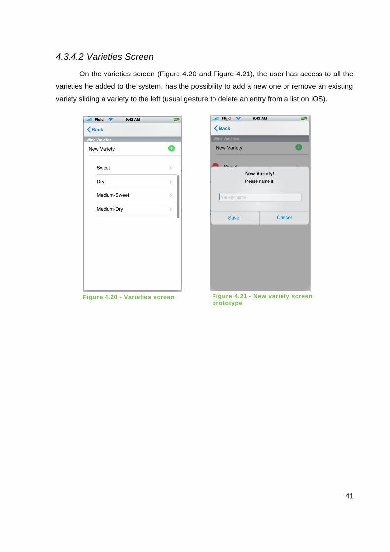
4.3.4.2 Varieties Screen
On the varieties screen (Figure 4.20 and Figure 4.21), the user has access to all the
varieties he added to the system, has the possibility to add a new one or remove an existing
variety sliding a variety to the left (usual gesture to delete an entry from a list on iOS).
Figure 4.20 - Varieties screen prototype
Figure 4.21 - New variety screen prototype

42
4.3.4.3 Base Samples Screen
This screen (Figure 4.22 and Figure 4.23) presents to the user all the known samples
he added to the system, indicating the variety that they belong to. Its functionalities are similar
to the ones presented on Home Screen. The user can delete a line from the list by sliding a
sample to the left, or can add a new one using the New Base Sample functionality.
Figure 4.22 - Base samples screen prototype
Figure 4.23 - Base samples screen
prototype, delete sample

43
4.3.4.4 New Base Sample Screens
This interface allows the user to create a new base sample. It starts by taking a photo
of a wine sample (Figure 4.24), then the user accepts the image if valid (Figure 4.25).
Figure 4.24 - New base sample, screen prototype
Figure 4.25 - New base sample,
use photo screen prototype

44
After capturing an image, the user names the sample (Figure 4.27) and then selects
from a list of varieties the one that matches that sample (Figure 4.26).
Figure 4.27 - Name new base
sample, screen prototype Figure 4.26 - New base sample, select variety screen prototype

45
4.3.4.5 New Test Screen
To create a new test, the interface is the same as the one to add a new Base Sample.
The user also enters the interface that has the inbuilt camera as shown in Figure 4.24,
accepts the captured image if valid as Figure 4.25 demonstrates and adds a name again as
he does for a new Base Sample in Figure 4.27.
After all these steps, the app calculates the matching variety and then presents the
result in the next interface.
4.3.4.6 Results Screen
In this screen presented in Figure 4.28, the results are presented as percentage. This
demonstrates how likely a sample is of a variety.
Figure 4.28 - Results screen prototype
46
4.3.5 FINAL INTERFACE AND EVOLUTION
After building the app with the new interface configuration, it was clear that it has some
usability problems. The location of some icons and links makes difficult to use the app when
operating with the 3D Prototype.
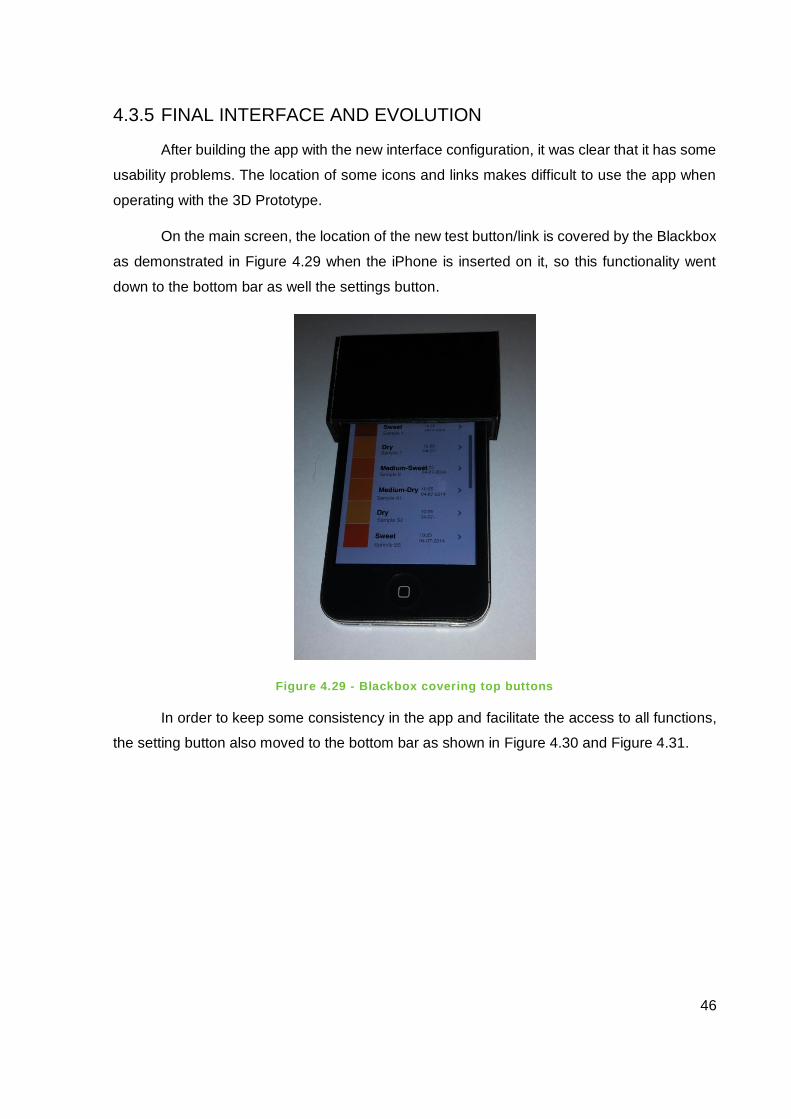
On the main screen, the location of the new test button/link is covered by the Blackbox
as demonstrated in Figure 4.29 when the iPhone is inserted on it, so this functionality went
down to the bottom bar as well the settings button.
Figure 4.29 - Blackbox covering top buttons
In order to keep some consistency in the app and facilitate the access to all functions,
the setting button also moved to the bottom bar as shown in Figure 4.30 and Figure 4.31.

47
This solution is much “cleaner” than the previous one, it has better appearance and
makes the entire navigation easier.
Figure 4.30 - Home Screen, final version
Figure 4.31 - Home screen, Settings final version

48
On the Base Samples screen, Figure 4.33, the changes had the same basis, access
the functionality when the device is inserted on the prototype, so the new base sample button
went down to the bottom bar.
The Varieties Screen, Figure 4.32, although it doesn’t require to use the prototype, it
was decided to use the same configuration as the other screens to keep consistency between
them, so the new variety button went down to the bottom bar.
Figure 4.33 - Base samples Screen,
final version Figure 4.32 - Varieties Screen, Final version

49
4.3.6 LESSONS LEARNED
The process of building the architecture for this project was not the usual one in
software engineering.
The project didn’t had a specific path to follow at the beginning. It was not possible to
build use cases, class diagrams, or even write the full list of requirements before start
developing the app.
The architecture was defined during the execution of the project and it was not defined
until the end of it. The development was based on programming a functionality, testing,
modifying if necessary and add new ones as new ideas were occurring during the
implementation.
The interface prototypes were also built as the project evolved and new functionalities
were added.
Has a consequence of the continuous development, the class diagram that is another
important element in software engineering, wasn’t also built before starting the development.
In this document is presented a version of the class diagram containing the main classes to
demonstrate the structure behind the app.
4.4 Software
The smartphone application is built to run on iPhone using iOS 7.x and was also
evolving continuously during the project as new features where created.
4.4.1 VERSION 1
The first version of the software created has its origin in the first tests made with all the
objects and color palettes.
The functionalities where very simple. It only allowed to take a photo and then click in
some point of the image so the software could print out the RGB values for that point and also
the average RGB value for the whole image. This test was made with wine and the paper
prototype created. The photos were taken inside home with artificial light, in full dark, and
outside with sun light.

50
One of the first steps to do before test for RGB values was to control the flash light
intensity. Using full flash, the upper half becomes white, and the lower half had the wine color.
After controlling the flash light intensity, the colour of the wine in the image became
more clear as demonstrated in Figure 4.34 in comparison with the image without controlling it
presented in Figure 4.4 that has a predominance of the white color induced by the flash light.
Figure 4.34 - Captured image with controlled flash light
In Figure 4.35, having the two situations side-by-side, on the left without controlling the
flash light, and on the right with the controlled flash light, it’s clear the improvement on the
image quality.

51
Figure 4.35 - Image comparison, with flash (left image) and without flash light (right image)
Clicking in some point and retrieve its color information for comparison purposes is not
enough, the images have many color variations because of the flash light and the shadow of
the container. The average RGB values for all the image are more precise, and, with this test,
we can notice from Table 4.4, Table 4.5 and Table 4.6 that the values don't change significantly
in all the different spaces, proving that the Blackbox prototype was working.
Some differences for the average RGB values between tests for the same sample at
this stage could be errors introduced from the paper prototype. This prototype was not very
stable, the recipient and the smartphone were moving inside it and affecting the results. This
problem was corrected when the 3D printed one was adjusted to perfectly fit both the iPhone
4S and the recipient.
Table 4.4 - Test inside home, normal light conditions
R G B
TEST 1 181 131 14
TEST 2 182 132 14
TEST 3 180 130 14
TEST 4 181 131 14
TEST 5 182 131 14

52
Table 4.5 - Test inside home, artificial light conditions
R G B
TEST 1 181 131 14
TEST 2 181 132 14
TEST 3 181 131 14
TEST 4 181 131 14
TEST 5 181 131 14
Table 4.6 - Test inside home, dark environment
4.4.2 VERSION 2
The second version is an improvement of how the color is measured and introduces
the image comparison methods.
After being able to measure the average RGB values on version 1, on this second
version it was recommended to find a more complete method to analyze the images. Following
Professor Mon-Chu recommendations to explore histograms, the next step was to do some
research on how they could be used to compare images.
The research quickly revealed a solution. There is a library that can be used to compare
images using Histograms that is called OpenCV [36].
R G B
TEST 1 181 131 14
TEST 2 181 130 14
TEST 3 181 131 14
TEST 4 180 130 14
TEST 5 182 132 14

53
OpenCV uses a series of comparison methods to measure the degree of similarity
(d(H1 and H2)) between two Hue-Saturation histograms (H1 and H2) generated from two
images. These four metrics are:
Correlation:
𝑑 (𝐻1, 𝐻2) =∑ (𝐻1(𝐼) − 𝐻1
)(𝐻2(𝐼) − 𝐻2 )𝐼
√∑ (𝐻1(𝐼) − 𝐻1 )2 ∑ (𝐻2(𝐼) − 𝐻2
)𝐼𝐼2
Were
𝐻𝑘 = 1
𝑁 ∑ 𝐻𝑘(𝐽)
𝐽
and 𝑁 is the total number of histogram bins.
Chi-Square:
𝑑 (𝐻1, 𝐻2) = ∑(𝐻1(𝐼) − 𝐻2(𝐼))2
𝐻1(𝐼)𝐼
Intersection:
𝑑 (𝐻1, 𝐻2) = ∑ min (𝐻1(𝐼), 𝐻2(𝐼))
𝐼
Bhattacharyya distance:
𝑑 (𝐻1, 𝐻2) = √1 − 1
√𝐻1𝐻2 𝑁2
∑ √𝐻1(𝐼) ⋅ 𝐻2(𝐼)
𝐼
For correlation and intersection, the higher the metric, the more accurate the match.
For Chi-Square and Bhattacharyya distance, the less the result, the better the match.
Starting from the base code from this library, this version was able to compare an image
from a photo captured at the moment with some previous selected and saved images, giving
as result the image that is most similar considering all the four methods.
This method is more accurate, because it uses four different metrics to analyze the
images instead of just comparing the Hue average value or only the RGB average values.
54
4.4.3 VERSION 3
The next step was to apply the histogram comparison techniques and adapt the
software to wine comparison.
Some features were added to the app:
Add and remove wine varieties: When this step was reached, it was clear that
the user should be able to manually introduce the wine varieties that he wants
to study, because they can change in the future, or accordingly to what the user
wants to test.
Add and remove base samples: The user as the possibility to add or remove
some known samples to the system in order to calibrate it. These samples are
images the user identifies as being from a given variety (already introduced in
the system), and they will be used in the future to compare against an unknown
sample that the system has to guess its variety.
To identify to which variety an unknown sample matches to, the system proceeds this
way:
1. Given a captured image from an unknown sample, and after labeling it with a
name, the system creates a counter for each variety in its list. This counter will
be used later to identify the variety with more matches.
2. Converts the image from RGB to HSV, that is the color space used by OpenCV
and calculates the Hue-Saturation histogram for the unknown sample.
3. Apply sequentially the four comparison methods between the Hue-Saturation
histogram of the captured image and the other Hue-Saturation histograms from
the known samples inserted into the system.
4. For each comparison method, for the image that matched the unknown one, the
system gets its variety and then, on the counter, it increments the value for that
variety.
5. Once finished all histogram comparisons, the system presents the result for each
counter that represents how much the given unknown sample matches each
variety, in a scale from 0% to 100%. The system can consider that a sample has
25% probability of being Medium-Sweet and 75% probability of being Medium-
Dry.

55
In Appendix 2, the scheme describes this process described above.
This new functionalities added more complexity to the system. Consequently, the
interface response started to slow down.
The main thread should be used only to update the user interface. All other
functionalities such as data loading, data processing, all that requires huge processing power
should be done in a separate thread.
The use of NSOperation and NSOperationQueue simplifies the process of
multithreading, the solution for this responsiveness problem. All the tasks or operations are an
instance of NSOperation class, and, NSOperationQueue class is responsible to start the
operations, ensure they run in the appropriate order, and take into account any priorities that
have been set [37].
The process for using NSOperatioQueue is the following:
1. Instantiate a new NSOperationQueue object
NSOperationQueue *queue = [NSOperationQueue new];
2. Create an instance of some NSOperation
NSInvocationOperation *operation = [[NSInvocationOperation alloc]
initWithTarget:selfselector:@selector(methodToCall)object:nil];
3. Add the operation to the queue
[queue addOperation:operation];
4. Release the operation
[operation release];
For this app, the process of analyzing the images and identify the variety is made in a
separate thread using this technique explained above.
Before multithreading use, when the user performed a test, the interface was locked in
the screen that requests the user for a name for that sample, from the beginning of the test
until the end.
This solution allowed to use the main thread to prepare the user interface to load the
results into, and also allowed to create a progress view, where the user gets feedback from
the system and verifies that the app is working as demonstrated in Figure 4.36. This user

56
interface updates were not possible before, because the main thread was locked in the image
processing.
Figure 4.36 - Processing feedback
4.4.4 VERSION 4
One of the main updates was the image sizes used in the app.
The test was initially done using a full size image, as captured from camera. This was
creating serious memory problems. The app reached some moments in which simply closed.
It was necessary to do some tests to know to which point the image size can be reduced
without affecting the final result. Also, it is recommended by Apple to avoid manipulate image
objects greater than 1024x1024px in size due to memory constraints [38].
In Appendix 1 – Image size tests, all the results in green indicate that the result is the
same for those image sizes. The result in red, for the sample L12084 Test B, indicates that for
the size 500x667px, the result is different.
One wrong result in a universe of 180 tests is not very problematic, but considering the
Table 4.7, the average size for an image with dimensions 500x667px and 600x800px is very
similar, and also the test time for these two sizes is also very similar, so, it was decided to use

57
the size 600x800px that proved to keep the same results as the original size and allows to
save lots of memory.
Table 4.7 - Image Size vs Test Time
Size (px) Average Size
(Megabytes)
Average Test
time (for each
image)
500X667 0,5 MB 0,040s
600x800 0,7 MB 0,050s
750x1000 1 MB 0,070s
2448x3264 9 MB 1,378s
4.4.5 FINAL IMPROVEMENTS
After finishing the coding, and with a working version, it was decided to do some
improvements on the software.
Review the code and do some “cleaning” was part of the job, but it was also necessary
to create a more efficient way to load and save the data contained in the app. Previous to this
improvement, the data was loaded once the user opened the app but it was only available for
the class that loaded the data, not a very practical approach since the loaded data is used in
almost all class.
The singleton pattern [26], it’s simple to implement and can be used in this situation,
where it’s only necessary to have an instance with a global point of access.
So, using this pattern, an instance of it is created when the app is loading, containing
all the app data loaded from memory. If some class needs that data, it has only to call the
instance of the class implementing the singleton pattern. As the data as already been loaded,
it doesn’t have to be loaded again, saving time and memory.
Making use of the functions already present at the base code contained on the project,
it can be detected when the app is closing. This is useful to save data, so, when the app closes,
automatically saves the data to memory.

58
4.5 Logo
For the logo creation it was intended to use some aspect related to wine, and something
specific to Madeira Wine.
The logo in Figure 4.37 includes the marks left on a table by a glass of wine [40] and
the name of the app using a similar font to the one originally used to stamp original Madeira
Wine bottles. The colors are also associated to Madeira Wine color variations.
Figure 4.37 - App logo
4.6 Splash screen
The splash screen (Figure 4.38) that appears when the app is loading includes the logo
and associations with University of Madeira and Madeira Interactive Technologies Institute.
Figure 4.38 - App splash screen

59
5 TESTS AND RESULTS
This chapter covers the tests, explains all the procedure together with demonstrative
photos, describes the wine samples used and also contains the results analysis.
5.1 Procedure
This section describes all the steps and material required to test a sample.
It’s necessary some laboratory equipment to simplify the process:
Pipette
Quartz test cell
Cotton swab
Distilled water
Paper towels
Blackbox prototype
Test cell lid
IPhone 4S with Madeira Wine Analyzer App
Wine samples
The use of this equipment doesn’t require specific formation, but it’s necessary to be
careful when handling it because some of this equipment is fragile.
The app must be set-up before the first test. The varieties to study must be inserted in
the system as well as the known samples. The process to capture an image for a known
sample is the same as the one to capture an image of a sample to test.
Following, there is an ordered sequence of steps with an associated image to illustrate
each procedure.

60
5.1.1 STEP 1
Place the wine in the quartz test cell without completely fill it, leaving enough space to
put the lid.
It’s easier to do this process using a pipette as demonstrated in Figure 5.1.
Figure 5.1 - Preparing a sample to test

61
5.1.2 STEP 2
After the recipient is properly capped, it’s necessary to clean its faces from any wine
residues or any fingerprints using a paper towel. To avoid the fingerprints, it’s recommended
to hold the recipient using the opaque faces.
Once the recipient is fully clean, it can be placed inside the Blackbox prototype with
one of the clear faces facing the open space where the camera will be as demonstrated in
Figure 5.2.
Figure 5.2 - Inserting the test cell in the Blackbox prototype
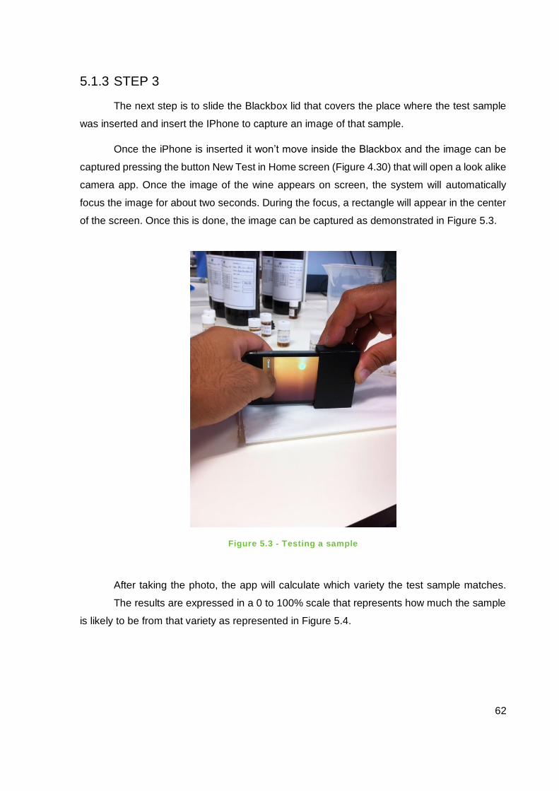
62
5.1.3 STEP 3
The next step is to slide the Blackbox lid that covers the place where the test sample
was inserted and insert the IPhone to capture an image of that sample.
Once the iPhone is inserted it won’t move inside the Blackbox and the image can be
captured pressing the button New Test in Home screen (Figure 4.30) that will open a look alike
camera app. Once the image of the wine appears on screen, the system will automatically
focus the image for about two seconds. During the focus, a rectangle will appear in the center
of the screen. Once this is done, the image can be captured as demonstrated in Figure 5.3.
Figure 5.3 - Testing a sample
After taking the photo, the app will calculate which variety the test sample matches.
The results are expressed in a 0 to 100% scale that represents how much the sample
is likely to be from that variety as represented in Figure 5.4.

63
Figure 5.4- Test results (Example)
5.2 Results Analysis
The tests were made with a total of 21 samples, the maximum number of different 3
year old wines available at the moment. From those, 6 are Dry, 2 Medium Dry, 6 Medium
Sweet and 7 are Sweet.
From the 21 samples, 11 were set as known samples in the app, that is, we take a
photo and identify the type of wine for calibration purposes. The choosing process was
completely random. The samples were on the table and 3 Dry samples, 1 Medium Dry, 3
Medium Sweet and 4 Sweet were separated as known samples. The other 10 were the test
samples, which the system didn’t knew anything about and had to test and guess the result.

64
Table 5.1 - Test results
Sample Test Expected Result Test Result
L13006 A
Dry Dry
B Dry
L12078 A
Dry Dry
B Dry
L12083 A
Dry Dry
B Dry
L12282 A
Medium Dry Medium Dry
B Medium Dry
L12079 A
Medium Sweet Medium Sweet
B Medium Sweet
L12108 A
Medium Sweet Medium Dry
B Medium Dry
L12076 A
Medium Sweet Medium Dry
B Medium Dry
L13363 A
Sweet Sweet
B Sweet
L12074 A
Sweet Sweet
B Sweet
L12075 A
Sweet Sweet
B Sweet
Analyzing the results on Table 5.1, the test results for the samples L12108 and L12076
were expected to be Medium Sweet and the system identified them as Medium Dry.
It’s expected that the system fails in some cases, because, there are so many wine
color variations, and some are very similar. This is a problem that can be diminished using
more known samples in the app.
As the problem is with the Medium Sweet samples, and the sample L12079 was
already correctly identified by the system, L12079 was added as known sample to test if any
of the incorrect results can now be correct.
The two incorrect test results are still incorrect. Again, one of the two samples that show
incorrect results was randomly chosen to set as known sample, in this case the sample
L12108.

65
A new test was made for the sample L12076, which resulted in a Medium Sweet wine,
a correct result.
This demonstrates how important calibration is. Adding another known sample
increased the fidelity of the system for this samples. This is a continuous process. On the next
production year, more 3 years old samples can be added to the system, and so on, to try to
reach a more perfect result. It doesn’t mean that the app will be 100% correct.
There is future work to do that is test more samples because 21 samples are not
enough, but that was the number available to test at the time.
The results were expectable and demonstrate potential in a future development of this
app.


67
6 CONCLUSIONS
The development of this project was a challenge from the beginning. It joined a difficult
scientific area like Chemistry with Software Engineering. It required some attention at the
beginning to understand the work that has been done at the lab and some totally unknown
concepts.
As this was not a standard project, that we know from the beginning which are the
requirements and we have a detailed plan and know what to expect, sometimes it was hard to
progress without losing some time thinking how some problem could be solved. This project
was a bit of trial, testing, correction, always discovering new solutions and improvements. The
fact that this was the first experience on the Apple environment, whether in the MAC OS, iOS
or even the programming language Objective-C highlighted even more this situation.
Sometimes, after finishing a section of code, that entire section was completely rebuilt because
a new and more efficient method was created. It’s expectable, because, starting from zero the
level of knowledge increased during the execution, and, as the efficiency and responsiveness
of the system are very important it worth it to update the coding.
Capturing a photo that has the same characteristics such as light conditions and
patterns affecting the image equally in all situations was the most important aspect to achieve.
A steady color reading is required to perform a comparison between images. They all need to
be captured under the same environment.
The device memory was another big concern since the beginning. Dealing with lots of
data may lead to problems when data volume increases. From the beginning that some
memory warnings where happening when testing the images for the histogram comparisons.
It was later noticed that the images where too large in pixels and Megabytes because they
were being used as captured, so it was necessary to re-dimension all the images when they
were captured.
The image resizing implementation took some time to do. On the first tries, the resized
image was losing quality, so it was necessary to find another way to do it that was achieved
after some research. After the resizing implementation it was clear that the tests were faster.
With the smaller image, a test that usually took about 1 minute is now done in a couple
of seconds. After solving the memory problem the concern was if resizing the image was
affecting the result, which proved not to be a problem for the size chosen that was 600x800px.

68
The application as room to grow in terms of reliability. The more known samples the
system has, more precise it will be because it has more references to compare to.
One limitation is the fact that the app only analyses the visible colors, and for that color
range, some wines appear to have the same color. For example, a medium-dry wine may be
similar to a medium-sweet as happened on the tests. The variety of colors that Madeira Wine
has as result of different ways of harvesting, fermentation and maturing process makes it more
difficult to test.
The idea was to use only a smartphone as far as possible, but, due to the environment
constraints presented on the work, such as light conditions, the creation of the 3D prototype
was inevitable. Although it’s an extra hardware to be used, the results indicate that the
prototype controlled the environment influence in the image.
The app only works when used together with the Blackbox device. It limits its use as it
requires an external device and not only the iPhone. The user has to carry the Blackbox with
him to perform a test, but, if the app is prepared to be used in the future in a winery for quality
control for example, that’s not a significant problem as the person who performs the tests will
be prepared with all the necessary equipment to test the samples.
The results for this experiment are good indicators for future works as the software is
able to analyze the color of a Madeira Wine sample, fulfilling the initial goal of preparing an
app for a smartphone to identify a Madeira wine by the color with a success rate of 80% to
90% on the performed tests as explained on the results analysis.

69
7 FUTURE WORK
Technology evolves every day. For example, the newer iPhone 5S has a more powerful
camera than the iPhone 4S used on this project and a different flash technology with two LED
called True Tone that allows to capture photos that look more natural adjusting variably the
color and intensity for 1000 combinations [41]. Now, by the ending of this project, the iPhone
6 has been released with even more processing capabilities. It never stops improving. Using
one of this new iPhones can improve the quality of the project.
The Blackbox used to put the recipient containing the wine inside, keeping it out from
light influence can be evolved to a most practical device. Maybe it’s is possible to find a solution
that allows to simplify the hardware, making it smaller or even discarding it completely,
although discarding it is a bit ambitious because of all the influences that the external
environment has on the test as demonstrated on this project.
If this application is prepared in the future to be launched for more users, it could benefit
from using cloud storage. This feature would provide a way for data sharing. For example, the
known samples can be shared by all the users, and, when a user adds one known sample to
the device, the other users can also receive that information to calibrate their system. It would
provide a collaborative way of testing samples. Also, users could have the possibility to save
their data so it won’t be lost if for some reason they lose the device or loose the data in device
software updates.
Some other features can be added to the app such as a detailed information about the
wine, curiosities, where to buy, etc. This could be for a commercial variation of this app directed
to general public. This can bring more interest around the wine.
As the iOS version as evolved on the final stage of this project from version 7 to 8, the
app has to be submitted to new tests to confirm if everything works. Apparently, there is no
problem with that, but only future testing can verify this.


71
8 REFERENCES
[1]. D. Forsyth and J. Ponce, Computer Vision: A Modern Approach. USA: Prentice Hall,
2003.
[2]. B. Tulsi (2014, May 01). “Good chemistry”, labmanager.com [Online]. Available:
http://goo.gl/f4bdQX [Accessed: 13-08-2014
[3]. W. Marten. “ColorMeter”, itunes.apple.com [Online]. Available: http://goo.gl/72ftvC
[Accessed: 01-10-2014]
[4]. Bioenos. “Colourimetric procedure to determine the color of wine from the grapes”,
bioenos.com [Online]. Available: http://goo.gl/G1RGZ8 [Accessed: 01-10-2014]
[5]. ETS Laboratories, ETS Wine Color Analysis. (2013). Available: http://goo.gl/vqrZb1
[Accessed: 01-10-2014]
[6]. Shimadzu UV-2600 UV-VIS spectrophotometer. [Online image]. Available:
http://goo.gl/8NiVDx [Accessed: 29-10-2014]
[7]. S. Slinkard. “Madeira Wine”, wine.about.com [Online]. Available: http://goo.gl/w0NyRs
[Accessed: 20-05-2014]
[8]. Madeira Wine Color [Online image]. Available: http://goo.gl/kf8n7J [Accessed: 21-05-
2014]
[9]. CCD Sensor [Online image]. Available: http://goo.gl/j2RfVm [Accessed: 05-11-2014]
[10]. Interpolation, Bayer filter pattern [Online image]. Available: http://goo.gl/bVVdiQ
[Accessed: 05-11-2014]
[11]. Bayer filter pattern [Online image]. Available: http://goo.gl/p31j7p [Accessed: 05-11-
2014]
[12]. Raw image vs processed image [Online image]. Available: http://goo.gl/MQ04C0
[Accessed: 05-11-2014]
[13]. K. Nice, T. V. Wilson and G. Gurevich. “How Digital Cameras Work”,
electronics.howstuffworks.com [Online]. Available: http://goo.gl/8Ckgkl [Accessed: 29-
05-2014]

72
[14]. D. N. Mendonza (2013, August 1). “A Tour of the Hardware Found in Modern
Smartphone Cameras”, PetaPixel [Online]. Available: http://goo.gl/XIr3Pz [Accessed:
29-05-2014]
[15]. R. Anderson and P. Krogh (2012, February 27). “Color space and color profiles”,
dpbestflow.org [Online]. Available: http://goo.gl/p7YO7z [Accessed: 29-05-2014]
[16]. S. Pappas (2010, April 29). “How do we see color?”, livescience.com [Online].
Available: http://goo.gl/JIWPFL [Accessed: 30-10-2014]
[17]. A. Z. Jones. “The Visible Light Spectrum”, physics.about.com [Online]. Available:
http://goo.gl/dQZcP4 [Accessed: 30-10-2014]
[18]. K. Tate. “How the eye sees in color”, National Library of Medicine [Online image].
Available: http://goo.gl/XL3hhA [Accessed: 30-10-2014]
[19]. “Color spaces”, [Online]. Available: http://goo.gl/N46ui5 [Accessed: 29-05-2014]
[20]. RGB cube, [Online image]. Available: http://goo.gl/t5M6fM [Accessed: 29-05-2014]
[21]. SpecialChem. “CIELab”, coatings.specialchem.com [Online]. Available:
http://goo.gl/CFyVV4 [Accessed: 22-08-2014]
[22]. J. Howard. “HSV”, About Tech [Online]. Available: http://goo.gl/mjBiAx [Accessed: 30-
05-2014]
[23]. HSV Cylinder. [Online image]. Available: http://goo.gl/XkkmfM [Accessed: 30-05-
2014]
[24]. OpenCV. “OpenCV - changing color spaces”, opencv.org [Online]. Available:
http://goo.gl/cX7DfJ [Accessed: 22-04-2014]
[25]. “3D printing basics”, blogspot.pt [Online]. Available: http://goo.gl/1xpU4r [Accessed:
21-05-2014]
[26]. K. Hall. “How 3D printing impacts manufacturing”, ComputerWeekly [Online].
Available: http://goo.gl/PkJon4 [Accessed: 28-10-2014]
[27]. Industry – 3D printed part [Online image]. Available: http://goo.gl/BqaKL2 [Accessed:
28-10-2014]
[28]. Laser printing [Online image]. Available: http://goo.gl/5EC9nl [Accessed: 28-10-2014]
[29]. CNC [Online image]. Available: http://goo.gl/iytZGI [Accessed: 28-10-2014]

73
[30]. T. Owad, (2014, March 17). “CNC Machining VS 3D Printing”, makezine.com [Online].
Available: http://goo.gl/dRGzZJ [Accessed: 28-10-2014]
[31]. Apple (2013). “Start Developing iOS Apps Today”, iOS Developer Library [Online].
Available: http://goo.gl/4eA5yK [Accessed: 30-09-2014]
[32]. Apple. “iOS development overview image”, iOS Developer Library [Online image].
Available: http://goo.gl/WubaxW [Accessed: 30-09-2014]
[33]. Apple. “XCode overview”, iOS Developer Library [Online image]. Available:
http://goo.gl/9FCx29 [Accessed: 30-09-2014]
[34]. Investopedia. “Histogram”, Investopedia.com [Online image]. Available:
http://goo.gl/1WdUtj [Accessed: 01-10-2014]
[35]. Histogram example. [Online image]. Available: http://goo.gl/w2mfzK [Accessed: 05-
10-2014]
[36]. OpenCV, “OpenCV – Histogram Comparison”, docs.opencv.org [Online]. Available:
http://goo.gl/MJtq9O [Accessed: 23-05-2014]
[37]. Brandontreb (2010, March 4). “iPhone Coding – Turbo Charging Your Apps With
NSOperation”, iCode [Online]. Available: http://goo.gl/peozbs [Accessed: 28-10-2014]
[38]. Apple. “UIImage”, iOS Developer Library [Online]. Available: http://goo.gl/5gLDpg
[Accessed: 10-08-2014]
[39]. Microsoft. “Singleton”, msdn.microsoft.com [Online]. Available: http://goo.gl/dGhdhM
[Accessed: 05-10-2014]
[40]. Wine glass marks. [Online image]. Available: http://goo.gl/dOkO83 [Accessed: 15-06-
2014]
[41]. Apple. “iPhone 5s”, apple.com [Online]. Available: http://goo.gl/UpFAa5 [Accessed:
19-08-2014]
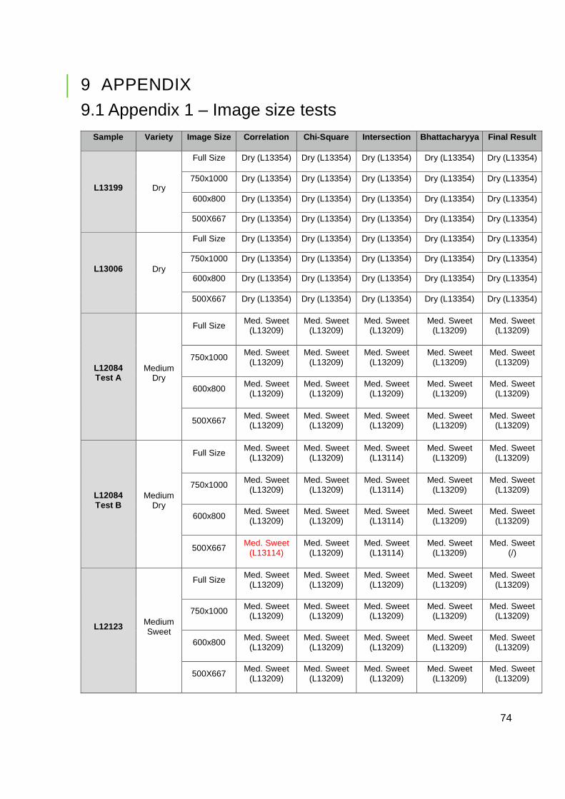
74
9 APPENDIX
9.1 Appendix 1 – Image size tests
Sample Variety Image Size Correlation Chi-Square Intersection Bhattacharyya Final Result
L13199 Dry
Full Size Dry (L13354) Dry (L13354) Dry (L13354) Dry (L13354) Dry (L13354)
750x1000 Dry (L13354) Dry (L13354) Dry (L13354) Dry (L13354) Dry (L13354)
600x800 Dry (L13354) Dry (L13354) Dry (L13354) Dry (L13354) Dry (L13354)
500X667 Dry (L13354) Dry (L13354) Dry (L13354) Dry (L13354) Dry (L13354)
L13006 Dry
Full Size Dry (L13354) Dry (L13354) Dry (L13354) Dry (L13354) Dry (L13354)
750x1000 Dry (L13354) Dry (L13354) Dry (L13354) Dry (L13354) Dry (L13354)
600x800 Dry (L13354) Dry (L13354) Dry (L13354) Dry (L13354) Dry (L13354)
500X667 Dry (L13354) Dry (L13354) Dry (L13354) Dry (L13354) Dry (L13354)
L12084 Test A
Medium Dry
Full Size Med. Sweet
(L13209) Med. Sweet
(L13209) Med. Sweet
(L13209) Med. Sweet
(L13209) Med. Sweet
(L13209)
750x1000 Med. Sweet
(L13209) Med. Sweet
(L13209) Med. Sweet
(L13209) Med. Sweet
(L13209) Med. Sweet
(L13209)
600x800 Med. Sweet
(L13209) Med. Sweet
(L13209) Med. Sweet
(L13209) Med. Sweet
(L13209) Med. Sweet
(L13209)
500X667 Med. Sweet
(L13209) Med. Sweet
(L13209) Med. Sweet
(L13209) Med. Sweet
(L13209) Med. Sweet
(L13209)
L12084 Test B
Medium Dry
Full Size Med. Sweet
(L13209) Med. Sweet
(L13209) Med. Sweet
(L13114) Med. Sweet
(L13209) Med. Sweet
(L13209)
750x1000 Med. Sweet
(L13209) Med. Sweet
(L13209) Med. Sweet
(L13114) Med. Sweet
(L13209) Med. Sweet
(L13209)
600x800 Med. Sweet
(L13209) Med. Sweet
(L13209) Med. Sweet
(L13114) Med. Sweet
(L13209) Med. Sweet
(L13209)
500X667 Med. Sweet
(L13114) Med. Sweet
(L13209) Med. Sweet
(L13114) Med. Sweet
(L13209) Med. Sweet
(/)
L12123 Medium Sweet
Full Size Med. Sweet
(L13209) Med. Sweet
(L13209) Med. Sweet
(L13209) Med. Sweet
(L13209) Med. Sweet
(L13209)
750x1000 Med. Sweet
(L13209) Med. Sweet
(L13209) Med. Sweet
(L13209) Med. Sweet
(L13209) Med. Sweet
(L13209)
600x800 Med. Sweet
(L13209) Med. Sweet
(L13209) Med. Sweet
(L13209) Med. Sweet
(L13209) Med. Sweet
(L13209)
500X667 Med. Sweet
(L13209) Med. Sweet
(L13209) Med. Sweet
(L13209) Med. Sweet
(L13209) Med. Sweet
(L13209)

75
L13363 Sweet
Full Size Sweet
(L13320) Sweet
(L13320) Sweet
(L13320) Sweet
(L13320) Sweet
(L13320)
750x1000 Sweet
(L13320) Sweet
(L13320) Sweet
(L13320) Sweet
(L13320) Sweet
(L13320)
600x800 Sweet
(L13320) Sweet
(L13320) Sweet
(L13320) Sweet
(L13320) Sweet
(L13320)
500X667 Sweet
(L13320) Sweet
(L13320) Sweet
(L13320) Sweet
(L13320) Sweet
(L13320)
L13117 Sweet
Full Size Med. Sweet
(L13114) Med. Sweet
(L13114) Med. Sweet
(L13114) Med. Sweet
(L13114) Med. Sweet
(L13114)
750x1000 Med. Sweet
(L13114) Med. Sweet
(L13114) Med. Sweet
(L13114) Med. Sweet
(L13114) Med. Sweet
(L13114)
600x800 Med. Sweet
(L13114) Med. Sweet
(L13114) Med. Sweet
(L13114) Med. Sweet
(L13114) Med. Sweet
(L13114)
500X667 Med. Sweet
(L13114) Med. Sweet
(L13114) Med. Sweet
(L13114) Med. Sweet
(L13114) Med. Sweet
(L13114)
L13198 test A
Sweet
Full Size Sweet
(L13236) Sweet
(L13236) Sweet
(L13236) Sweet
(L13236) Sweet
(L13236)
750x1000 Sweet
(L13236) Sweet
(L13236) Sweet
(L13236) Sweet
(L13236) Sweet
(L13236)
600x800 Sweet
(L13236) Sweet
(L13236) Sweet
(L13236) Sweet
(L13236) Sweet
(L13236)
500X667 Sweet
(L13236) Sweet
(L13236) Sweet
(L13236) Sweet
(L13236) Sweet
(L13236)
L13198 test B
Sweet
Full Size Sweet
(L13320) Sweet
(L13320) Sweet
(L13320) Sweet
(L13320) Sweet
(L13320)
750x1000 Sweet
(L13320) Sweet
(L13320) Sweet
(L13320) Sweet
(L13320) Sweet
(L13320)
600x800 Sweet
(L13320) Sweet
(L13320) Sweet
(L13320) Sweet
(L13320) Sweet
(L13320)
500X667 Sweet
(L13320) Sweet
(L13320) Sweet
(L13320) Sweet
(L13320) Sweet
(L13320)

76
9.2 Appendix 2 – Image comparison flowchart

77
9.3 Appendix 3 – How the Eye Sees in Color [18]