1

The Use of Collinearity Diagnostics in PK Model

Building

Gregory H. Michels

Purdue Pharma

2

• Introduction - Definitions

• Types of Collinearity

• Diagnosing Collinearity

• Conclusions

7KH�8VH�RI�&ROOLQHDULW\�'LDJQRVWLFV�LQ�3.�0RGHO�%XLOGLQJ

3

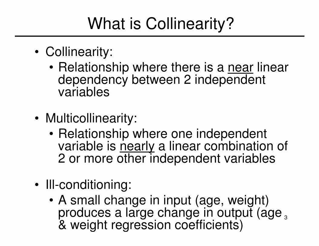
• Collinearity:

• Relationship where there is a near linear dependency between 2 independent variables

• Multicollinearity:

• Relationship where one independent variable is nearly a linear combination of 2 or more other independent variables

• Ill-conditioning:

• A small change in input (age, weight) produces a large change in output (age & weight regression coefficients)

What is Collinearity?

4

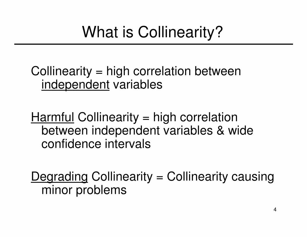
Collinearity = high correlation between independent variables

Harmful Collinearity = high correlation between independent variables & wide confidence intervals

Degrading Collinearity = Collinearity causing minor problems

What is Collinearity?

5

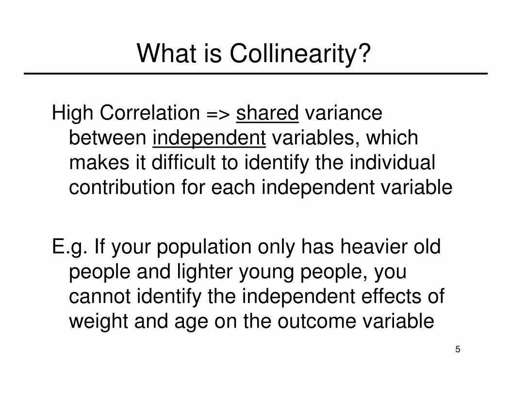
High Correlation => shared variance

between independent variables, which

makes it difficult to identify the individual

contribution for each independent variable

E.g. If your population only has heavier old

people and lighter young people, you

cannot identify the independent effects of

weight and age on the outcome variable

What is Collinearity?

6

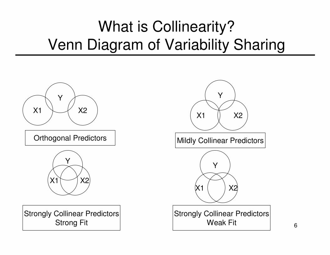
Y

X2X1

Orthogonal Predictors

X1 X2

Y

Mildly Collinear Predictors

Strongly Collinear Predictors

Weak Fit

Y

X2X1 X1

Y

X2

Strongly Collinear Predictors

Strong Fit

What is Collinearity?

Venn Diagram of Variability Sharing

7

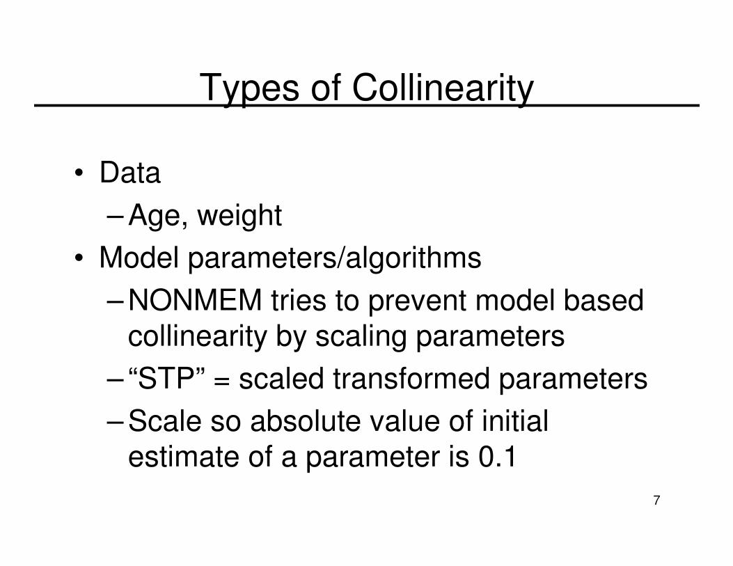
Types of Collinearity

• Data

– Age, weight

• Model parameters/algorithms

– NONMEM tries to prevent model based

collinearity by scaling parameters

– “STP” = scaled transformed parameters

– Scale so absolute value of initial

estimate of a parameter is 0.1

8

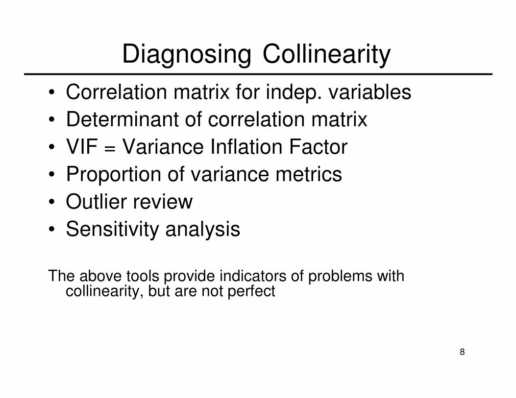
• Correlation matrix for indep. variables

• Determinant of correlation matrix

• VIF = Variance Inflation Factor

• Proportion of variance metrics

• Outlier review

• Sensitivity analysis

The above tools provide indicators of problems with collinearity, but are not perfect

Diagnosing Collinearity

9

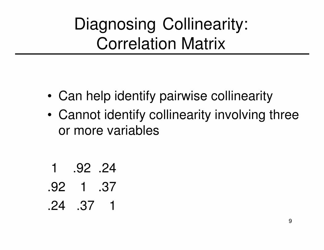
Diagnosing Collinearity: Correlation Matrix

• Can help identify pairwise collinearity

• Cannot identify collinearity involving three

or more variables

1 .92 .24

.92 1 .37

.24 .37 1

10

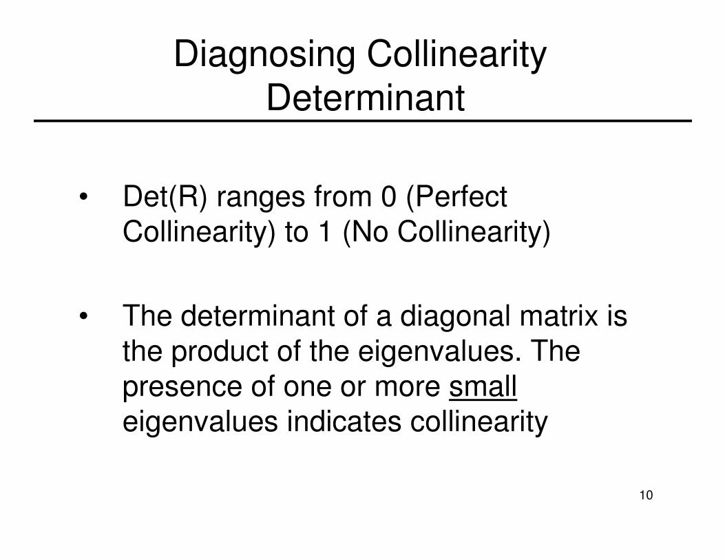
• Det(R) ranges from 0 (Perfect

Collinearity) to 1 (No Collinearity)

• The determinant of a diagonal matrix is

the product of the eigenvalues. The

presence of one or more small

eigenvalues indicates collinearity

Diagnosing CollinearityDeterminant

11

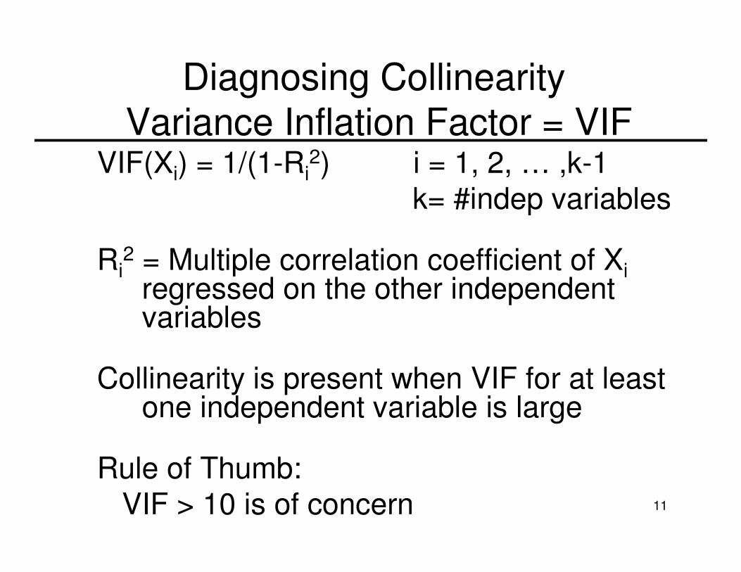
VIF(Xi) = 1/(1-Ri2) i = 1, 2, … ,k-1

k= #indep variables

Ri2 = Multiple correlation coefficient of Xi

regressed on the other independent variables

Collinearity is present when VIF for at least one independent variable is large

Rule of Thumb:

VIF > 10 is of concern

Diagnosing CollinearityVariance Inflation Factor = VIF

12

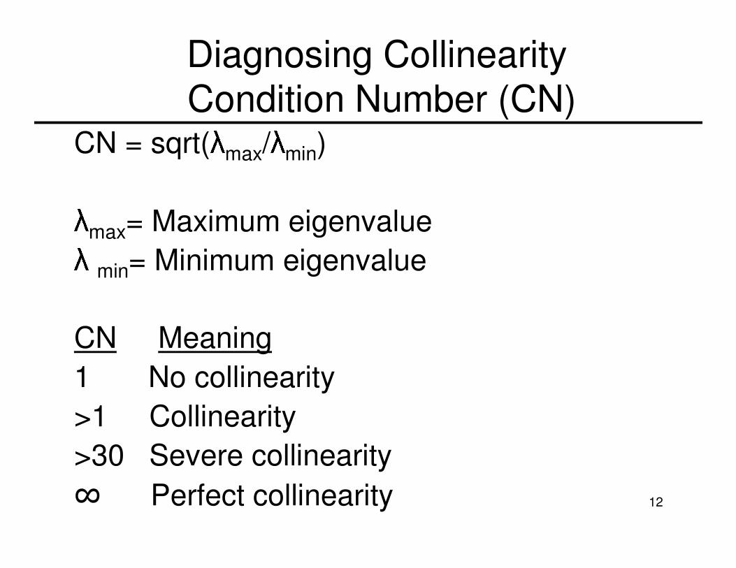
CN = sqrt( max/ min)

max= Maximum eigenvalue

min= Minimum eigenvalue

CN Meaning

1 No collinearity

>1 Collinearity

>30 Severe collinearity

� Perfect collinearity

Diagnosing CollinearityCondition Number (CN)

13

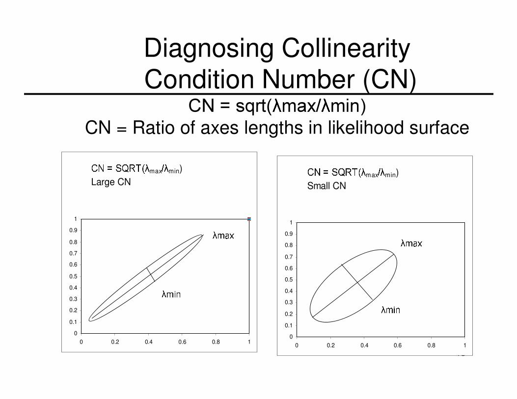
Diagnosing CollinearityCondition Number (CN)

&1� �VTUW� PD[� PLQ�CN = Ratio of axes lengths in likelihood surface

0

0.1

0.2

0.3

0.4

0.5

0.6

0.7

0.8

0.9

1

0 0.2 0.4 0.6 0.8 1

&1� �6457� max� min)

Small CN

PD[

PLQ

0

0.1

0.2

0.3

0.4

0.5

0.6

0.7

0.8

0.9

1

0 0.2 0.4 0.6 0.8 1

&1� �6457� max� min)

Large CN

PD[

PLQ

14

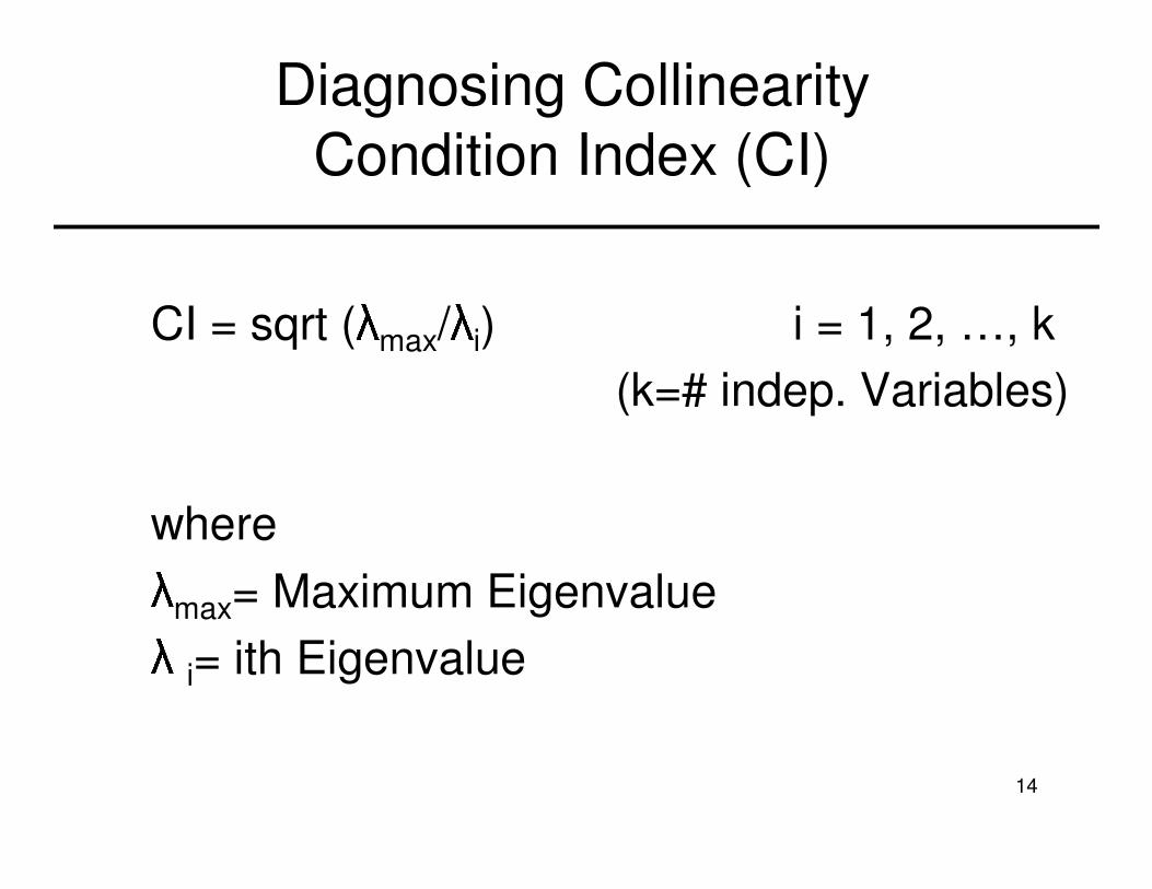
CI = sqrt ( max/ i) i = 1, 2, …, k

(k=# indep. Variables)

where

max= Maximum Eigenvalue

i= ith Eigenvalue

Diagnosing CollinearityCondition Index (CI)

15

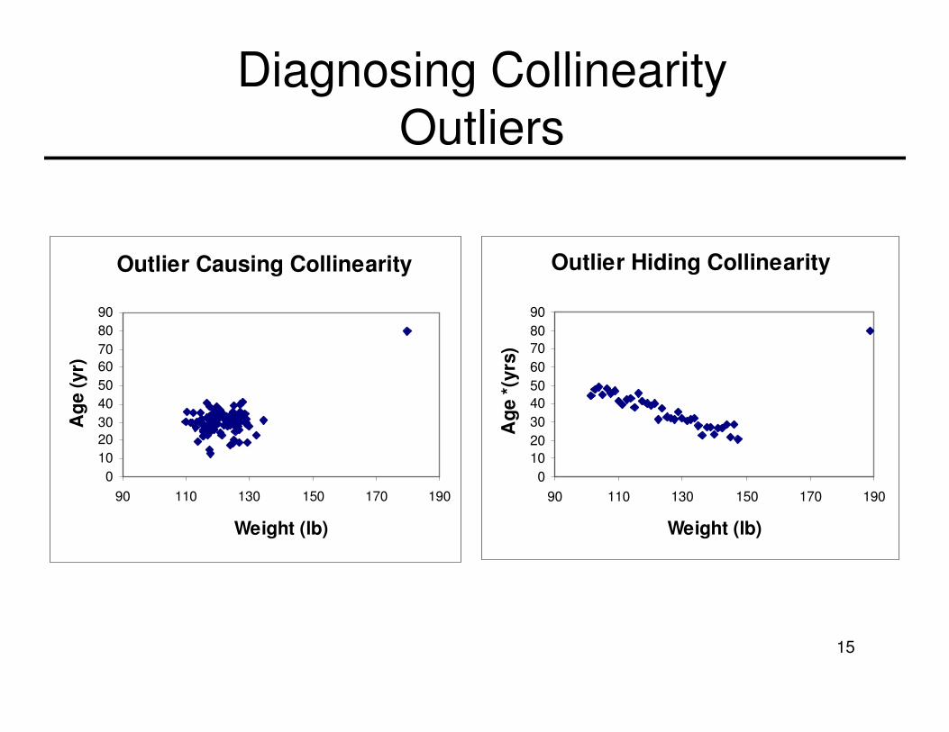
Diagnosing CollinearityOutliers

Outlier Hiding Collinearity

0

10

20

30

40

50

60

70

80

90

90 110 130 150 170 190

Weight (lb)A

ge *

(yrs

)

Outlier Causing Collinearity

0

10

20

30

40

50

60

70

80

90

90 110 130 150 170 190

Weight (lb)

Ag

e (

yr)

16

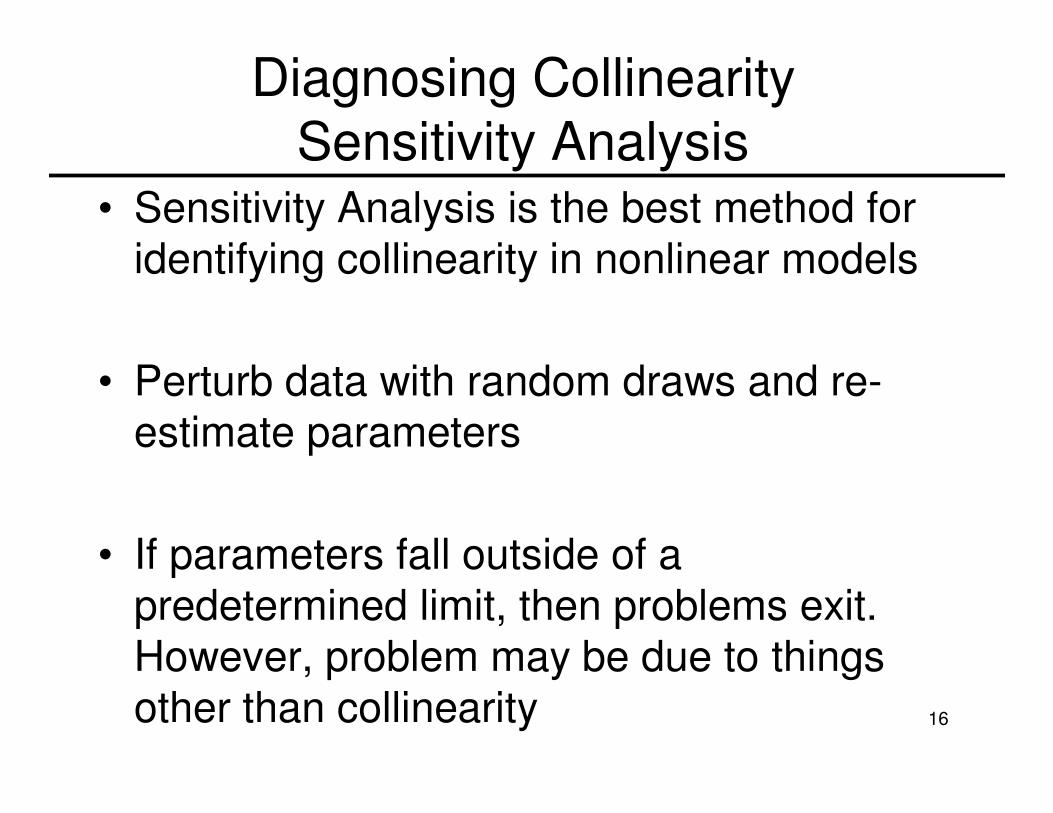
• Sensitivity Analysis is the best method for

identifying collinearity in nonlinear models

• Perturb data with random draws and re-

estimate parameters

• If parameters fall outside of a

predetermined limit, then problems exit.

However, problem may be due to things

other than collinearity

Diagnosing CollinearitySensitivity Analysis

17

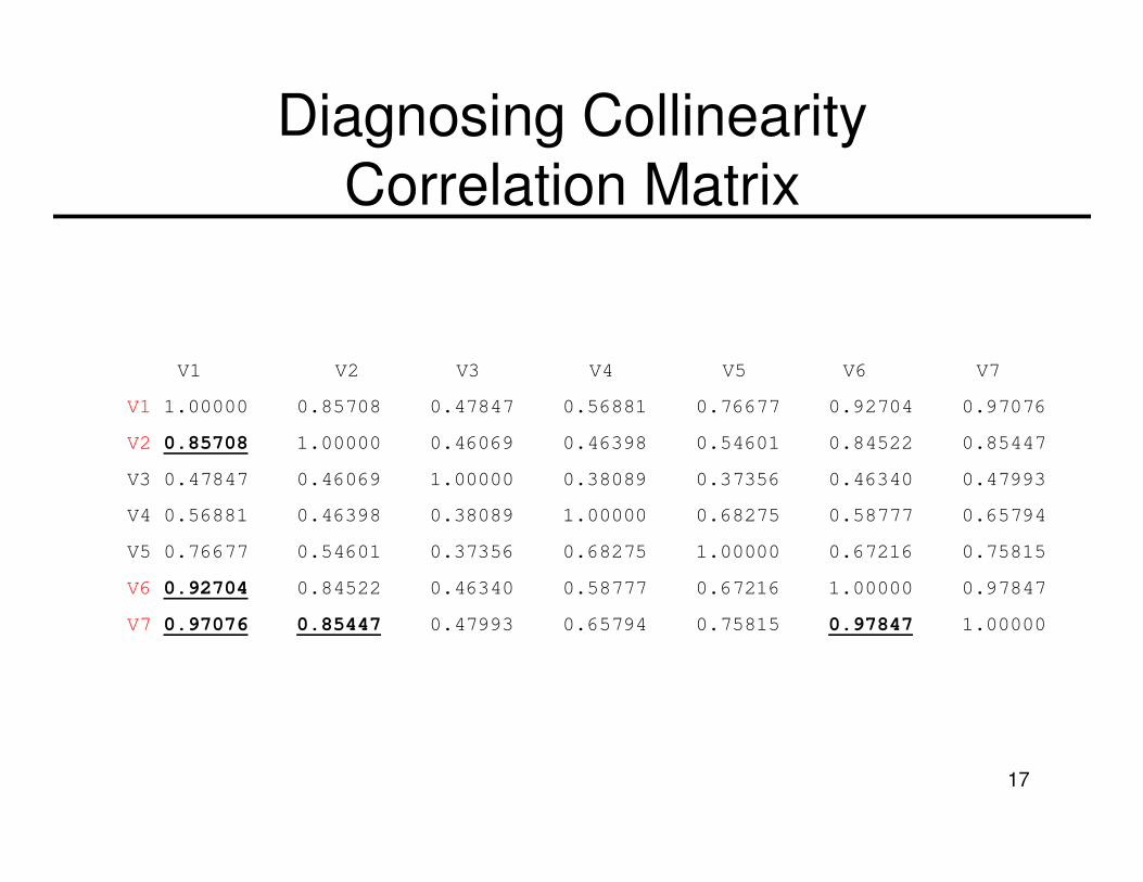
Diagnosing CollinearityCorrelation Matrix

V1 V2 V3 V4 V5 V6 V7

V1 1.00000 0.85708 0.47847 0.56881 0.76677 0.92704 0.97076

V2 0.85708 1.00000 0.46069 0.46398 0.54601 0.84522 0.85447

V3 0.47847 0.46069 1.00000 0.38089 0.37356 0.46340 0.47993

V4 0.56881 0.46398 0.38089 1.00000 0.68275 0.58777 0.65794

V5 0.76677 0.54601 0.37356 0.68275 1.00000 0.67216 0.75815

V6 0.92704 0.84522 0.46340 0.58777 0.67216 1.00000 0.97847

V7 0.97076 0.85447 0.47993 0.65794 0.75815 0.97847 1.00000

18

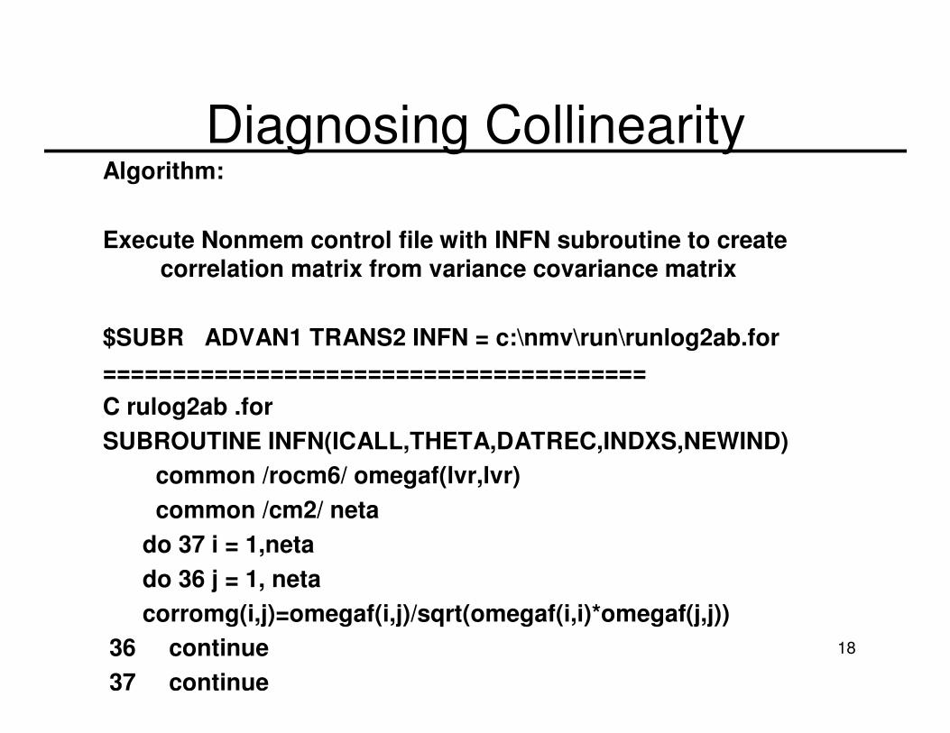
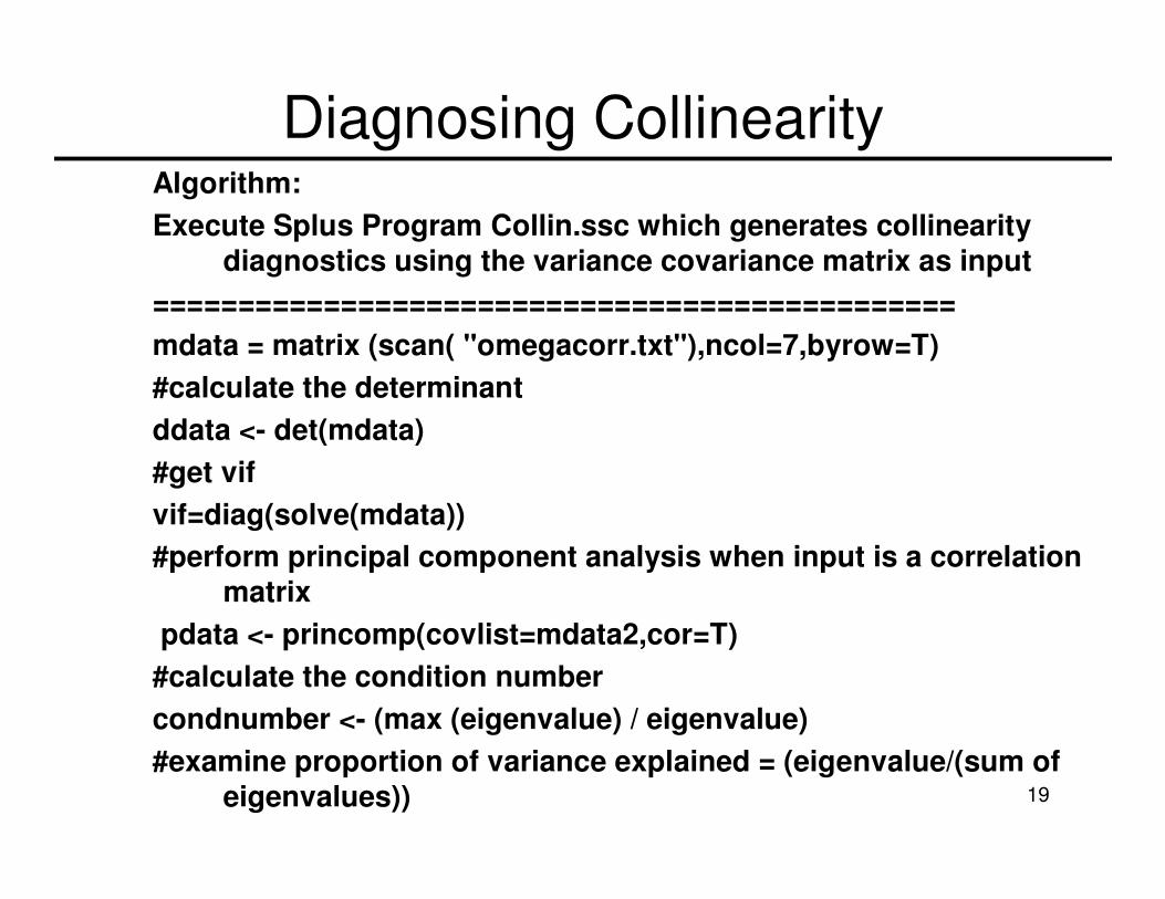
Diagnosing CollinearityAlgorithm:

Execute Nonmem control file with INFN subroutine to create correlation matrix from variance covariance matrix

$SUBR ADVAN1 TRANS2 INFN = c:\nmv\run\runlog2ab.for

=======================================

C rulog2ab .for

SUBROUTINE INFN(ICALL,THETA,DATREC,INDXS,NEWIND)

common /rocm6/ omegaf(lvr,lvr)

common /cm2/ neta

do 37 i = 1,neta

do 36 j = 1, neta

corromg(i,j)=omegaf(i,j)/sqrt(omegaf(i,i)*omegaf(j,j))

36 continue

37 continue

19

Diagnosing CollinearityAlgorithm:

Execute Splus Program Collin.ssc which generates collinearity diagnostics using the variance covariance matrix as input

===============================================

mdata = matrix (scan( "omegacorr.txt"),ncol=7,byrow=T)

#calculate the determinant

ddata <- det(mdata)

#get vif

vif=diag(solve(mdata))

#perform principal component analysis when input is a correlation matrix

pdata <- princomp(covlist=mdata2,cor=T)

#calculate the condition number

condnumber <- (max (eigenvalue) / eigenvalue)

#examine proportion of variance explained = (eigenvalue/(sum of eigenvalues))

20

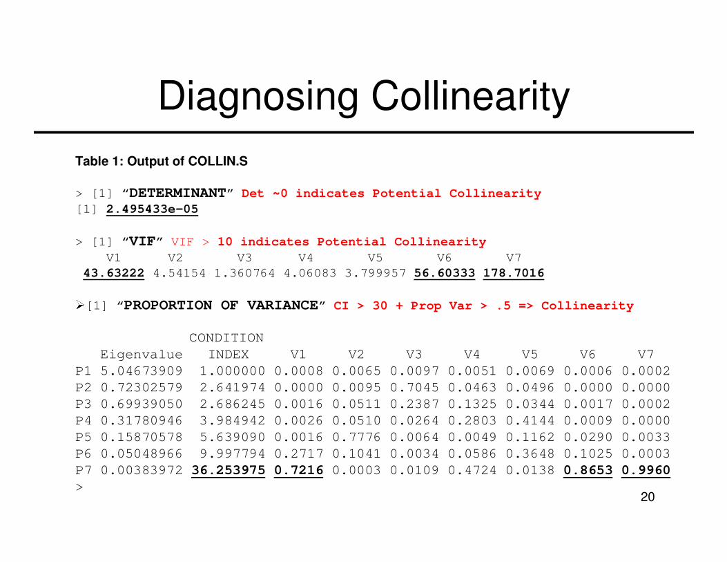
Diagnosing Collinearity

Table 1: Output of COLLIN.S

> [1] “DETERMINANT” Det ~0 indicates Potential Collinearity

[1] 2.495433e-05

> [1] “VIF” VIF > 10 indicates Potential Collinearity

V1 V2 V3 V4 V5 V6 V7

43.63222 4.54154 1.360764 4.06083 3.799957 56.60333 178.7016

¾[1] “PROPORTION OF VARIANCE” CI > 30 + Prop Var > .5 => Collinearity

CONDITION

Eigenvalue INDEX V1 V2 V3 V4 V5 V6 V7

P1 5.04673909 1.000000 0.0008 0.0065 0.0097 0.0051 0.0069 0.0006 0.0002

P2 0.72302579 2.641974 0.0000 0.0095 0.7045 0.0463 0.0496 0.0000 0.0000

P3 0.69939050 2.686245 0.0016 0.0511 0.2387 0.1325 0.0344 0.0017 0.0002

P4 0.31780946 3.984942 0.0026 0.0510 0.0264 0.2803 0.4144 0.0009 0.0000

P5 0.15870578 5.639090 0.0016 0.7776 0.0064 0.0049 0.1162 0.0290 0.0033

P6 0.05048966 9.997794 0.2717 0.1041 0.0034 0.0586 0.3648 0.1025 0.0003

P7 0.00383972 36.253975 0.7216 0.0003 0.0109 0.4724 0.0138 0.8653 0.9960

>

21

Conclusions

• Identifying collinearity problems in NONMEM output can be difficult

• Correlation matrix derived from NONMEM output does not provide sufficient information

22

Conclusions• The determinant, VIF, and proportion

of variance matrix pinpoint the specific variables with collinearity problems that should be removed from the next run

• Examine collinearity diagnostics andregression coefficient confidence intervals to determine if collinearity is harmful

23

References

•Belsely, DA, Kuh, E., & Welsch, RE 1980.

Regression diagnostics: Identifying influential data

and sources of collinearity. New York

•Bonate, Peter 2006. Pharmacokinetic-

Pharmacodynamic Modeling and Simulation.

Springer, New York

•Mason, RL, & Gunst, RF Outlier-Induced

Collinearities Technometrics, Vol. 27, No. 4 (Nov.,

1985) , pp. 401-407