Cohesive Zone Model-ref
27
INTERNA TIONAL JOURNAL FOR NUMERICAL METHODS IN ENGINEERING Int. J. Numer . Meth. Engng 2004; 60:289–315 (DOI: 10.1002/nme.963) Cohesiv e-zone models, higher-order continuum theories and reliability methods for computational failure analysis ‡ René de Borst ∗, † , Miguel A. Gutiérrez, Garth N. Wells, Joris J. C. Remmers and Harm Askes Koi ter Inst itute Delft , Delft Univer sity of Techno logy , P .O. Box 5058 , NL- 2600 GB Delft , The Nethe rland s SUMMARY A concise overview is given of various numerical methods that can be used to analyse localization and failure in engineering materials. The importance of the cohesive-zone approach is emphasized and var ious way s to incor porat e the cohe siv e-zone metho dolog y in discr etiza tion metho ds are disc usse d. Numerical rep res entations of coh esi ve-zone mod els suf fer from a certain mesh bia s. For dis cre te rep res entations this is cau sed by the ini tial mes h des ign, while for sme are d rep resentations it is roote d in the ill-p osedn ess of the rate bound ary value problem that arises upon the intro ducti on of deco hesio n. A prope r repre sentation of the disc rete char acter of cohes ive-zone formulati ons which av oids any mesh bias can be obtai ned elegant ly when exploi ting the parti tion-o f-uni ty prope rty of finite element shape functions. The effectiveness of the approach is demonstrated for some examples at different scales. Moreover, examples are shown how this concept can be used to obtain a proper transition from a plastifying or damaging continuum to a shear band with gross sliding or to a fully open crack (true discont inuum). When adhering to a conti nuum descript ion of failu re, higher-o rder continuum models must be used. Meshless methods are ideally suited to assess the importance of the highe r-or der gradi ent terms , as will be shown. Final ly , regu lariz ed strai n-sof tenin g models are used in finite element reliability analyses to quantify the probability of the emergence of various possible failure modes. Copyright 2004 John Wiley & Sons, Ltd. KEY WORDS: loca lizat ion; failu re; cohes iv e zones; disco ntinu ities ; higher- order cont inua; part ition s of unity; meshless methods; reliability methods; imperfections 1. INTR ODUCTION Failure in most engineering materials is preceded by the emergence of narrow zones of intense straining. During this phase of the so-called strain localization, the deformation pattern in a body rather suddenly changes from relatively smooth into one in which thin zones of highly ∗ Cor res pon dence to: Ren é de Borst, Ko ite r Ins tit ute Del ft, Delft Uni ver sit y of T echnol ogy , P.O. Box 505 8, NL-2 600 GB Delft , The Nethe rland s. † E-mail:[email protected] ‡ Revised version of semi- plena ry lectur e pres ented at the Fifth World Congres s on Comp utational Mechanics under the origi nal title ‘A Précis of Some Recent Dev elopments in Comp utati onal Failure Mechanics ’. Received 10 May 2003 Copyright 2004 John Wiley & Sons, Ltd. Acce pted 25 Jul y 2003
-
Upload
elizabeth-santiago -
Category
Documents
-
view
230 -
download
0
Transcript of Cohesive Zone Model-ref

8/11/2019 Cohesive Zone Model-ref
http://slidepdf.com/reader/full/cohesive-zone-model-ref 1/27
INTERNATIONAL JOURNAL FOR NUMERICAL METHODS IN ENGINEERING Int. J. Numer. Meth. Engng 2004; 60:289–315 (DOI: 10.1002/nme.963)
Cohesive-zone models, higher-order continuum theories and
reliability methods for computational failure analysis‡
René de Borst∗,†, Miguel A. Gutiérrez, Garth N. Wells,Joris J. C. Remmers and Harm Askes
Koiter Institute Delft , Delft University of Technology, P.O. Box 5058, NL-2600 GB Delft , The Netherlands
SUMMARY
A concise overview is given of various numerical methods that can be used to analyse localizationand failure in engineering materials. The importance of the cohesive-zone approach is emphasized andvarious ways to incorporate the cohesive-zone methodology in discretization methods are discussed.Numerical representations of cohesive-zone models suffer from a certain mesh bias. For discreterepresentations this is caused by the initial mesh design, while for smeared representations it isrooted in the ill-posedness of the rate boundary value problem that arises upon the introduction of decohesion. A proper representation of the discrete character of cohesive-zone formulations whichavoids any mesh bias can be obtained elegantly when exploiting the partition-of-unity property of finite element shape functions. The effectiveness of the approach is demonstrated for some examplesat different scales. Moreover, examples are shown how this concept can be used to obtain a propertransition from a plastifying or damaging continuum to a shear band with gross sliding or to a fullyopen crack (true discontinuum). When adhering to a continuum description of failure, higher-ordercontinuum models must be used. Meshless methods are ideally suited to assess the importance of thehigher-order gradient terms, as will be shown. Finally, regularized strain-softening models are used
in finite element reliability analyses to quantify the probability of the emergence of various possiblefailure modes. Copyright 2004 John Wiley & Sons, Ltd.
KEY WORDS: localization; failure; cohesive zones; discontinuities; higher-order continua; partitionsof unity; meshless methods; reliability methods; imperfections
1. INTRODUCTION
Failure in most engineering materials is preceded by the emergence of narrow zones of intense
straining. During this phase of the so-called strain localization, the deformation pattern in a
body rather suddenly changes from relatively smooth into one in which thin zones of highly
∗Correspondence to: René de Borst, Koiter Institute Delft, Delft University of Technology, P.O. Box 5058,NL-2600 GB Delft, The Netherlands.
†E-mail:[email protected]‡Revised version of semi-plenary lecture presented at the Fifth World Congress on Computational Mechanicsunder the original title ‘A Précis of Some Recent Developments in Computational Failure Mechanics’.
Received 10 May 2003
Copyright 2004 John Wiley & Sons, Ltd. Accepted 25 July 2003

8/11/2019 Cohesive Zone Model-ref
http://slidepdf.com/reader/full/cohesive-zone-model-ref 2/27
290 R. DE BORST ET AL.
strained material dominate. In fact, these strain localization zones act as a precursor to ultimate
fracture and failure. Thus, in order to accurately analyse the failure behaviour of materials it
is of pivotal importance that the strain localization phase is modelled in a physically consistent
and mathematically correct manner and that proper numerical tools are used.
Until the mid-1980s analyses of localization phenomena in materials were commonly carriedout using standard, rate-independent continuum models. This is reasonable when the principal
aim is to determine the behaviour in the pre-localization regime and some properties at incipient
localization. However, there is a major difficulty in the post-localization regime, since localiza-
tion in standard, rate-independent solids is intimately related to a local change in the character
of the governing set of partial differential equations. Upon this change of character, the rate
boundary value problem becomes ill-posed and numerical solutions suffer from spurious mesh
sensitivity.
To remedy this deficiency, one must either introduce higher-order terms in the continuum
representation or take into account the inherent viscosity of most engineering materials. An
alternative possibility is to by-pass the strain localization phase and to directly incorporate the
discontinuity that arises as an outcome of the strain localization process. The latter possibility is
pursued with the so-called cohesive-zone models. We will start by describing them and discuss
how they can be introduced in a numerical context. We will argue that finite elements with
‘embedded’ localization zones do not rigorously incorporate discontinuities in finite element
models. Conversely, finite element formulations that exploit the partition-of-unity property of the
shape functions [1] can, as will be discussed. Indeed, this concept also enables the modelling of
a gradual transition from a (higher-order) continuum description to a genuine discontinuum in a
numerical context. This is very powerful, since now the entire failure process, from small-scale
yielding or the initiation of voids and micro-cracks up to the formation of a macroscopically
observable crack, can be simulated in a consistent and natural fashion.
Like for finite element methods, the shape functions of meshless discretizations, e.g. the
element-free Galerkin method [2], form partitions of unity. Meshless methods have a tremen-
dous advantage for models in which higher-order terms are incorporated, since they inherentlyprovide for the required higher-order continuity. Accordingly, enhanced continuum models can
be implemented easily and the importance of the higher-order gradients can be assessed.
Finally, we will indicate how the heterogeneous character of materials at a macroscopic
scale can be incorporated in numerical analyses of inelastic solids. In particular, the effect of
stochastically distributed imperfections on the failure load in inelastic solids will be quantified
in the framework of the finite element reliability method.
2. COHESIVE-ZONE MODELS
2.1. Formulation
An important issue when considering failure is the observation that most engineering materials
are not perfectly brittle in the Griffith sense, but display some ductility after reaching the
strength limit. In fact, there exists a small zone in front of the crack tip, in which small-
scale yielding, micro-cracking and void initiation, growth and coalescence take place. If this
fracture process zone is sufficiently small compared to the structural dimensions, linear-elastic
fracture mechanics concepts apply. However, if this is not the case, the cohesive forces that
Copyright 2004 John Wiley & Sons, Ltd. Int. J. Numer. Meth. Engng 2004; 60:289–315

8/11/2019 Cohesive Zone Model-ref
http://slidepdf.com/reader/full/cohesive-zone-model-ref 3/27
COMPUTATIONAL FAILURE ANALYSIS 291
cohesive zone
Figure 1. Schematic representation of a cohesive zone.
σ
u
t
σ
f t
u
Figure 2. Stress–displacement curves for a ductile solid (left) and a quasi-brittle solid (right).
exist in this fracture process zone must be taken into account, and cohesive-zone models must
be used, which were introduced by Barenblatt [3] and Dugdale [4] for elastic–plastic fracture in
ductile metals, and for quasi-brittle materials by Hillerborg et al. [5] in his so-called fictitiouscrack model.
In cohesive-zone models, the degrading mechanisms in front of the actual crack tip are
lumped into a discrete line or plane (Figure 1) and a stress–displacement relationship across
this line or plane represents the degrading mechanisms in the fracture process zone. Figure 2
shows some commonly used decohesion relations, one for ductile fracture (left) [6] and one
for quasi-brittle fracture (right) [7]. For ductile fracture, the most important parameters of the
cohesive zone model appear to be the tensile strength f t and the work of separation or fracture
energy Gc [8], which is the work needed to create a unit area of fully developed crack. It has
the dimensions J/m2 and is formally defined as
Gc
= du (1)
with and u being the stress and the displacement across the fracture process zone. For more
brittle decohesion relations, as shown for instance in the right part of Figure 2 (i.e. when
the decohesion law stems from micro-cracking as in concrete or ceramics), the shape of the
stress–separation relation plays a much bigger role and is sometimes even more important than
the value of the tensile strength f t [9, 10].
Copyright 2004 John Wiley & Sons, Ltd. Int. J. Numer. Meth. Engng 2004; 60:289–315

8/11/2019 Cohesive Zone Model-ref
http://slidepdf.com/reader/full/cohesive-zone-model-ref 4/27
292 R. DE BORST ET AL.
Figure 3. Geometry of single-edged notched (SEN) beam.
Figure 4. Deformed configuration of the SEN-beam that results from an analysis where inter-face elements equipped with a quasi-brittle cohesive-zone model have been placed a priori at the
experimentally known crack path [12].
2.2. Discrete numerical representations of cohesive-zone models
In the past two decades, cohesive-zone models have been recognized to be an important tool
for describing fracture in engineering materials. Especially when the crack path is known in
advance, either from experimental evidence, or because of the structure of the material (such
as in laminated composites), cohesive-zone models have been used with great success. In those
cases, the mesh can be constructed such that the crack path a priori coincides with the element
boundaries. By inserting interface elements between continuum elements along the potential
crack path, a cohesive crack can be modelled exactly. Figures 3 and 4 show this for mixed-modefracture in a single-edge notched (SEN) concrete beam [11]. In this example the mesh has been
designed such that the interface elements, which are equipped with a quasi-brittle cohesive-
zone model, are exactly located at the position of the experimentally observed crack path [12].
Another good example where the potential of cohesive-zone models can be exploited fully using
traditional discrete interface elements, e.g. Reference [13], is the analysis of delamination in
layered composite materials [14–17]. Since the propagation of delaminations is then restricted
Copyright 2004 John Wiley & Sons, Ltd. Int. J. Numer. Meth. Engng 2004; 60:289–315
8/11/2019 Cohesive Zone Model-ref
http://slidepdf.com/reader/full/cohesive-zone-model-ref 5/27
COMPUTATIONAL FAILURE ANALYSIS 293
to the interfaces between the plies, inserting interface elements at these locations permits an
exact simulation of the failure mode.
To allow for a more arbitrary direction of crack propagation, Xu and Needleman [18]
have inserted interface elements equipped with a cohesive-zone model between all continuum
elements. A related method, using remeshing, was proposed by Camacho and Ortiz [19].Although analyses with this approach provide much insight, see also References [20, 21], they
suffer from a certain mesh bias, since the direction of crack propagation is not entirely free, but
is restricted to interelement boundaries. Another drawback is that the method is not suitable for
large-scale analyses. For these two reasons smeared numerical representations of cohesive-zone
models have appeared, including the emergence of some, initially unforeseen mathematical
difficulties, which can only be overcome in a rigorous fashion by resorting to higher-order
continuum models.
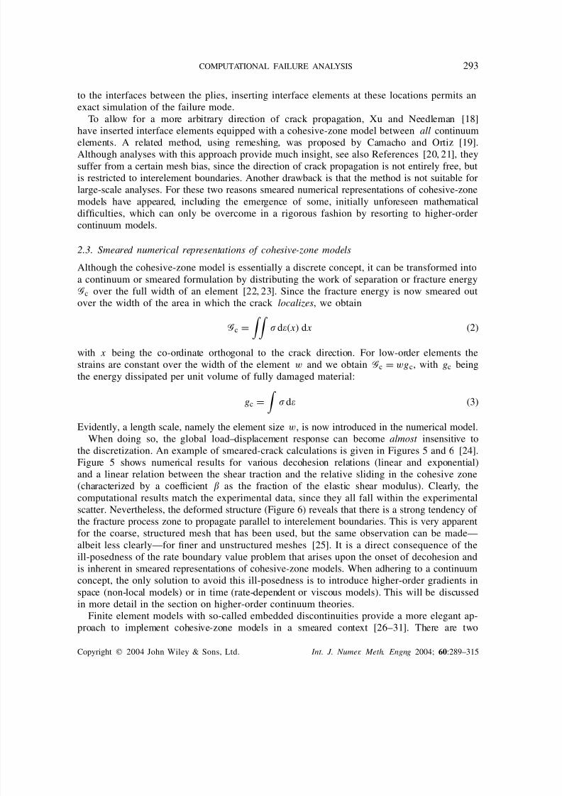
2.3. Smeared numerical representations of cohesive-zone models
Although the cohesive-zone model is essentially a discrete concept, it can be transformed into
a continuum or smeared formulation by distributing the work of separation or fracture energyGc over the full width of an element [22, 23]. Since the fracture energy is now smeared out
over the width of the area in which the crack localizes, we obtain
Gc =
d(x) dx (2)
with x being the co-ordinate orthogonal to the crack direction. For low-order elements the
strains are constant over the width of the element w and we obtain Gc = wgc, with gc being
the energy dissipated per unit volume of fully damaged material:
gc = d (3)
Evidently, a length scale, namely the element size w, is now introduced in the numerical model.
When doing so, the global load–displacement response can become almost insensitive to
the discretization. An example of smeared-crack calculations is given in Figures 5 and 6 [24].
Figure 5 shows numerical results for various decohesion relations (linear and exponential)
and a linear relation between the shear traction and the relative sliding in the cohesive zone
(characterized by a coefficient as the fraction of the elastic shear modulus). Clearly, the
computational results match the experimental data, since they all fall within the experimental
scatter. Nevertheless, the deformed structure (Figure 6) reveals that there is a strong tendency of
the fracture process zone to propagate parallel to interelement boundaries. This is very apparent
for the coarse, structured mesh that has been used, but the same observation can be made—
albeit less clearly—for finer and unstructured meshes [25]. It is a direct consequence of the
ill-posedness of the rate boundary value problem that arises upon the onset of decohesion andis inherent in smeared representations of cohesive-zone models. When adhering to a continuum
concept, the only solution to avoid this ill-posedness is to introduce higher-order gradients in
space (non-local models) or in time (rate-dependent or viscous models). This will be discussed
in more detail in the section on higher-order continuum theories.
Finite element models with so-called embedded discontinuities provide a more elegant ap-
proach to implement cohesive-zone models in a smeared context [26–31]. There are two
Copyright 2004 John Wiley & Sons, Ltd. Int. J. Numer. Meth. Engng 2004; 60:289–315

8/11/2019 Cohesive Zone Model-ref
http://slidepdf.com/reader/full/cohesive-zone-model-ref 6/27
294 R. DE BORST ET AL.
Figure 5. Load–CMSD curves for the SEN-beam that result from analyses with asmeared cohesive-zone model [24].
Figure 6. Deformed configuration of the SEN-beam that results from an analysiswith a smeared cohesive-zone model [24].
versions of these models, namely the strong discontinuity approach and the weak discontinuity
approach. We will depart from the latter approach and consider an element within which a
band is defined where the strains are different in magnitude from the strains in the remainder
of the element:
−ij = ij +
−
2(nimj + nj mi) (4)
and
+ij = ij +
+
2(nimj + nj mi) (5)
with n a vector normal to the band and m related to the deformation mode, e.g. m = n
for mode-I behaviour and n orthogonal to m for mode-II behaviour. − and + are scalars
Copyright 2004 John Wiley & Sons, Ltd. Int. J. Numer. Meth. Engng 2004; 60:289–315
8/11/2019 Cohesive Zone Model-ref
http://slidepdf.com/reader/full/cohesive-zone-model-ref 7/27
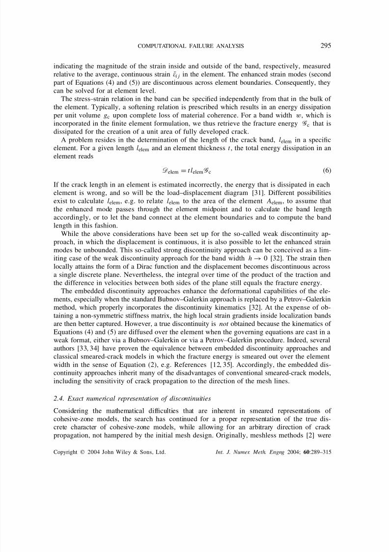
COMPUTATIONAL FAILURE ANALYSIS 295
indicating the magnitude of the strain inside and outside of the band, respectively, measured
relative to the average, continuous strain ij in the element. The enhanced strain modes (second
part of Equations (4) and (5)) are discontinuous across element boundaries. Consequently, they
can be solved for at element level.
The stress–strain relation in the band can be specified independently from that in the bulk of the element. Typically, a softening relation is prescribed which results in an energy dissipation
per unit volume gc upon complete loss of material coherence. For a band width w, which is
incorporated in the finite element formulation, we thus retrieve the fracture energy Gc that is
dissipated for the creation of a unit area of fully developed crack.
A problem resides in the determination of the length of the crack band, lelem in a specific
element. For a given length lelem and an element thickness t , the total energy dissipation in an
element reads
Delem = t lelemGc (6)
If the crack length in an element is estimated incorrectly, the energy that is dissipated in each
element is wrong, and so will be the load–displacement diagram [31]. Different possibilitiesexist to calculate lelem, e.g. to relate lelem to the area of the element Aelem, to assume that
the enhanced mode passes through the element midpoint and to calculate the band length
accordingly, or to let the band connect at the element boundaries and to compute the band
length in this fashion.
While the above considerations have been set up for the so-called weak discontinuity ap-
proach, in which the displacement is continuous, it is also possible to let the enhanced strain
modes be unbounded. This so-called strong discontinuity approach can be conceived as a lim-
iting case of the weak discontinuity approach for the band width h → 0 [32]. The strain then
locally attains the form of a Dirac function and the displacement becomes discontinuous across
a single discrete plane. Nevertheless, the integral over time of the product of the traction and
the difference in velocities between both sides of the plane still equals the fracture energy.
The embedded discontinuity approaches enhance the deformational capabilities of the ele-ments, especially when the standard Bubnov–Galerkin approach is replaced by a Petrov–Galerkin
method, which properly incorporates the discontinuity kinematics [32]. At the expense of ob-
taining a non-symmetric stiffness matrix, the high local strain gradients inside localization bands
are then better captured. However, a true discontinuity is not obtained because the kinematics of
Equations (4) and (5) are diffused over the element when the governing equations are cast in a
weak format, either via a Bubnov–Galerkin or via a Petrov–Galerkin procedure. Indeed, several
authors [33, 34] have proven the equivalence between embedded discontinuity approaches and
classical smeared-crack models in which the fracture energy is smeared out over the element
width in the sense of Equation (2), e.g. References [12, 35]. Accordingly, the embedded dis-
continuity approaches inherit many of the disadvantages of conventional smeared-crack models,
including the sensitivity of crack propagation to the direction of the mesh lines.
2.4. Exact numerical representation of discontinuities
Considering the mathematical difficulties that are inherent in smeared representations of
cohesive-zone models, the search has continued for a proper representation of the true dis-
crete character of cohesive-zone models, while allowing for an arbitrary direction of crack
propagation, not hampered by the initial mesh design. Originally, meshless methods [2] were
Copyright 2004 John Wiley & Sons, Ltd. Int. J. Numer. Meth. Engng 2004; 60:289–315

8/11/2019 Cohesive Zone Model-ref
http://slidepdf.com/reader/full/cohesive-zone-model-ref 8/27
296 R. DE BORST ET AL.
thought as the answer to this problem, but they appear to be less robust than traditional finite
element methods, they are computationally more demanding and the implementation in three
dimensions appears to be less straightforward. However, out of this research, a method has
emerged recently, in which a discontinuity in the displacement field is captured exactly. It has
the added benefit that it can be used advantageously at different scales, from microscopic tomacroscopic analyses.
The method makes use of the partition-of-unity property of finite element shape functions
[1,36,37]. A collection of functions i , associated with nodes i, form a partition of unity if
ni=1
i(x) = 1 (7)
with n being the number of discrete nodal points. For a set of functions i that satisfy Equation
(7), a field u can be interpolated as follows:
u(x) =
ni=1i(
x)ai +
mj =1j (
x)aij
(8)
with ai the ‘regular’ nodal degrees-of-freedom, j (x) the enhanced basis terms, and aij the
additional degrees-of-freedom at node i which represent the amplitudes of the j -th enhanced
basis term j (x).
A piecewise continuous displacement field u which incorporates a discontinuity with a unit
normal vector n pointing in an arbitrary, but fixed direction can be described by
u(x) = u(x) + Hd(x)u(x) (9)
with u the standard, continuous displacement field on which the discontinuity has been super-
imposed. The discontinuous field is represented by the continuous field u and the Heaviside
function Hd , centred at the discontinuity plane d. The displacement decomposition in Equa-tion (9) has a structure similar to the interpolation of Equation (8). Accordingly, the partition-
of-unity property of finite element shape functions can be used in a straightforward fashion
to incorporate discontinuities, and thus, cohesive-zone models in a manner that preserves their
truly discontinuous character. Indeed, in conventional finite element notation, the displacement
field of an element that contains a single discontinuity can be represented as
u = N(a + Hda) = Na + Hd
Na = u + Hd u (10)
where N contains the standard shape functions, and a and a collect the conventional and
the additional nodal degrees-of-freedom, respectively. The numerical development now follows
standard lines by casting the balance of momentum in a weak format, and, in the spirit
of a standard Bubnov–Galerkin method, taking a decomposition as in Equation (9) also forthe test function. For small displacement gradients a complete derivation can be found in
Reference [38], while the extension to large displacement gradients is given in Reference [39].
It is interesting to note that, at variance with requirements for the ‘embedded’ displacement
discontinuity approaches, the field u does not have to be constant. The only requirement that
is imposed is continuity. Therefore, a distinction can be made between the normals n−d
and
n+d
at both sides of the discontinuity (Figure 7). It is this distinction that allows for capturing
Copyright 2004 John Wiley & Sons, Ltd. Int. J. Numer. Meth. Engng 2004; 60:289–315

8/11/2019 Cohesive Zone Model-ref
http://slidepdf.com/reader/full/cohesive-zone-model-ref 9/27
COMPUTATIONAL FAILURE ANALYSIS 297
nΓ d
n
+
−
Γ d
Figure 7. Normals n−d
and n+d
at both sides of the discontinuity.
local buckling at the interface. An example involving the combination of delamination and
local buckling will be given below.It is emphasized that in this concept, the additional degrees-of-freedom cannot be condensed
at element level, because, at variance with the ‘embedded’ displacement discontinuity approach,
it is node-oriented and not element-oriented. It is this property which makes it possible to
represent a discontinuity in a rigorous manner.
From Equations (8) and (10) we infer that the partition-of-unity concept can naturally be
conceived as a multiscale approach [40]. We can formally show this by decomposing u(x) as
u(x) = uC(x) + uF(x) (11)
with
uC(x) =
ni=1i(x)ai (12)
representing the coarse scale and
uF(x) =ni=1
mj =1
i(x)j (x)aij (13)
representing the fine scale.
The objectivity of the formulation with respect to mesh refinement is demonstrated for the
three-point bending beam of unit thickness shown in Figure 8. The beam is loaded quasi-
statically by means of an imposed displacement at the centre of the beam on the top edge.
Six-noded triangular elements are used as the underlying base elements. The following material
properties have been used: Young’s modulus E = 100 MPa, Poisson’s ratio = 0.0, tensilestrength f t = 1.0 MPa and fracture energy Gc = 0.1 Jmm−2. For this example, the crack shear
stiffness is set equal to zero. Since the crack shear stiffness vanishes, the top row of elements
of the beam have been prevented from cracking in order to avoid singularity of the system
when the crack has propagated through the entire beam.
Figure 9 shows the crack having propagated through the entire beam. Two meshes are
shown, one with 523 elements and the other with 850 elements. Clearly, in both cases the
Copyright 2004 John Wiley & Sons, Ltd. Int. J. Numer. Meth. Engng 2004; 60:289–315

8/11/2019 Cohesive Zone Model-ref
http://slidepdf.com/reader/full/cohesive-zone-model-ref 10/27
298 R. DE BORST ET AL.
3
55
P
Figure 8. Geometry of a beam subjected to symmetric three-point bending (dimensions in mm).
Figure 9. Crack path at the final stage of loading for the coarse mesh (523 elements) and thefine mesh (850 elements) [38].
crack propagates from the centre at the bottom of the beam straight upwards towards the load
point, not influenced by the mesh structure.
The load–displacement responses of Figure 10 confirm objectivity with respect to meshrefinement. From the load–displacement response for the coarser mesh the energy dissipation is
calculated as 0.308 J, which only slightly exceeds the fracture energy multiplied by the depth
and the thickness of the beam (0.3 J), giving further proof of mesh objectivity. It is further
noted that the small irregularities that are observed in the load–displacement curve, especially
for the coarser mesh, are caused by the fact that in the current implementation a cohesive
zone is inserted entirely in one element when the tensile strength has been exceeded. A more
Copyright 2004 John Wiley & Sons, Ltd. Int. J. Numer. Meth. Engng 2004; 60:289–315

8/11/2019 Cohesive Zone Model-ref
http://slidepdf.com/reader/full/cohesive-zone-model-ref 11/27
COMPUTATIONAL FAILURE ANALYSIS 299
Figure 10. Load–displacement diagrams for the analysis of the symmetrically loadedbeam using both meshes [38].
Figure 11. Crack path that results from the analysis of the SEN-beam using the partition-of-unityproperty of finite element shape functions [38].
sophisticated way is to advance the crack only in a part of the element, for instance using level
sets [41, 42]. However, the observation that these little bumps quickly disappear upon mesh
refinement (Figure 10) casts doubt on the necessity to complicate the numerical model.
Usually, the requirement that the crack path is not biased by the direction of the mesh lines
is even more demanding than the requirement of objectivity with respect to mesh refinement.
Figure 11 shows that the approach also fully satisfies this requirement, since the numerically
predicted crack path of the single edge notched beam of Figure 3 is in excellent agreement
with experimental observations, e.g. Reference [11].
Even though traditional interface elements equipped with cohesive-zone models are able tocapture the failure behaviour of laminated composites accurately, the simulation of delami-
nation using the partition-of-unity property of finite element shape functions offers some ad-
vantages. Because the discontinuity does not have to be inserted a priori, no (dummy) stiffness
is needed in the elastic regime. Indeed, there does not have to be an elastic regime, since
the discontinuity can be activated at the onset of cracking. Consequently, the issue of spurious
traction oscillations in the elastic phase becomes irrelevant. Also, the lines of the potential
Copyright 2004 John Wiley & Sons, Ltd. Int. J. Numer. Meth. Engng 2004; 60:289–315

8/11/2019 Cohesive Zone Model-ref
http://slidepdf.com/reader/full/cohesive-zone-model-ref 12/27
300 R. DE BORST ET AL.
Figure 12. Double cantilever beam with initial delamination under compression.
Debonding (coarse mesh)
Debonding (dense mesh)Perfect bond
P [ N ]
1 2 3 4 5 6 7 8
u (mm )
0
1
2
3
4
Figure 13. Load–displacement curves for delamination-buckling test [43].
delamination planes no longer have to coincide with element boundaries. They can lie at
arbitrary locations inside elements. Accordingly, unstructured meshes can be used.
To exemplify the possibilities of this approach to model the combined failure mode of de-
lamination growth and local buckling we consider the double cantilever beam of Figure 12 with
an initial delamination length a. This case, in which failure is a consequence of a combination
of delamination growth and structural instability, has been analysed using conventional interface
elements in Reference [17]. The beam is subjected to an axial compressive force 2P , while
two small perturbing forces P 0 are applied to trigger the buckling mode. Two finite element
discretizations have been employed, a fine mesh with three elements over the thickness and250 elements along the length of the beam, and a coarse mesh with only one (!) element over
the thickness and 100 elements along the length. Figure 13 shows that the calculation with
the coarse mesh approaches the results for the fine mesh closely. For instance, the numeri-
cally calculated buckling load is in good agreement with the analytical solution. Steady-state
delamination growth starts around a lateral displacement u = 4 mm. From this point onwards,
delamination growth interacts with geometrical instability. Figure 14 presents the deformed
Copyright 2004 John Wiley & Sons, Ltd. Int. J. Numer. Meth. Engng 2004; 60:289–315

8/11/2019 Cohesive Zone Model-ref
http://slidepdf.com/reader/full/cohesive-zone-model-ref 13/27
COMPUTATIONAL FAILURE ANALYSIS 301
Figure 14. Deformation of coarse mesh after buckling and delamination growth (true scale) [43].
Figure 15. Load–displacement curve and deformations of shell model after buckling anddelamination growth (true scale) [43].
beam for the coarse mesh at a tip displacement u = 6 mm. Note that the displacements are
plotted at true scale, but that the difference in displacement between the upper and lower parts
of the beam is for the major part due to the delamination and that the strains remain small.
The excellent results obtained in this example for the coarse discretization has motivated
the development of a layered plate/shell element in which delaminations can occur inside
the element between each of the layers [43]. Because of the absence of rotational degrees
of freedom, a solid-like shell element [44] was taken as a point of departure. The numerical
results of Figure 15 show an excellent correspondence with the earlier two-dimensional resultsof Figures 13 and 14. This opens the possibility to analyse delamination-buckling in thin-walled
composite structures at a structural scale.
In all examples discussed above, a single, continuous cohesive crack growth was simulated.
Crack propagation in heterogeneous materials and also fast crack growth in more homogeneous
materials is often characterized by the nucleation of (micro)cracks at several locations, which can
grow, branch and eventually link up to form macroscopically observable cracks. To accommodate
Copyright 2004 John Wiley & Sons, Ltd. Int. J. Numer. Meth. Engng 2004; 60:289–315
8/11/2019 Cohesive Zone Model-ref
http://slidepdf.com/reader/full/cohesive-zone-model-ref 14/27
302 R. DE BORST ET AL.
this observation, the concept of cohesive segments has been proposed [45], in which, again
exploiting the partition-of-unity property of finite element shape functions, crack segments
equipped with a cohesive law are placed over a patch of elements when a loading criterion
is met at an integration point. Since the cohesive segments can overlap in elements, they can
also behave macroscopically as a single, dominant crack.
3. CONTINUUM–DISCONTINUUM TRANSITION
The above approach enables the gradual and consistent transition from a continuum to a
discontinuum description. In Reference [46] traction-free discontinuities have been inserted in
a softening, viscoplastic Von Mises plasticity model when the equivalent plastic strain reaches
a threshold level. Accordingly, the viscosity of the continuum has been used to ensure a mesh-
independent result in the softening phase prior to local failure and the creation of a traction-free
discontinuity.
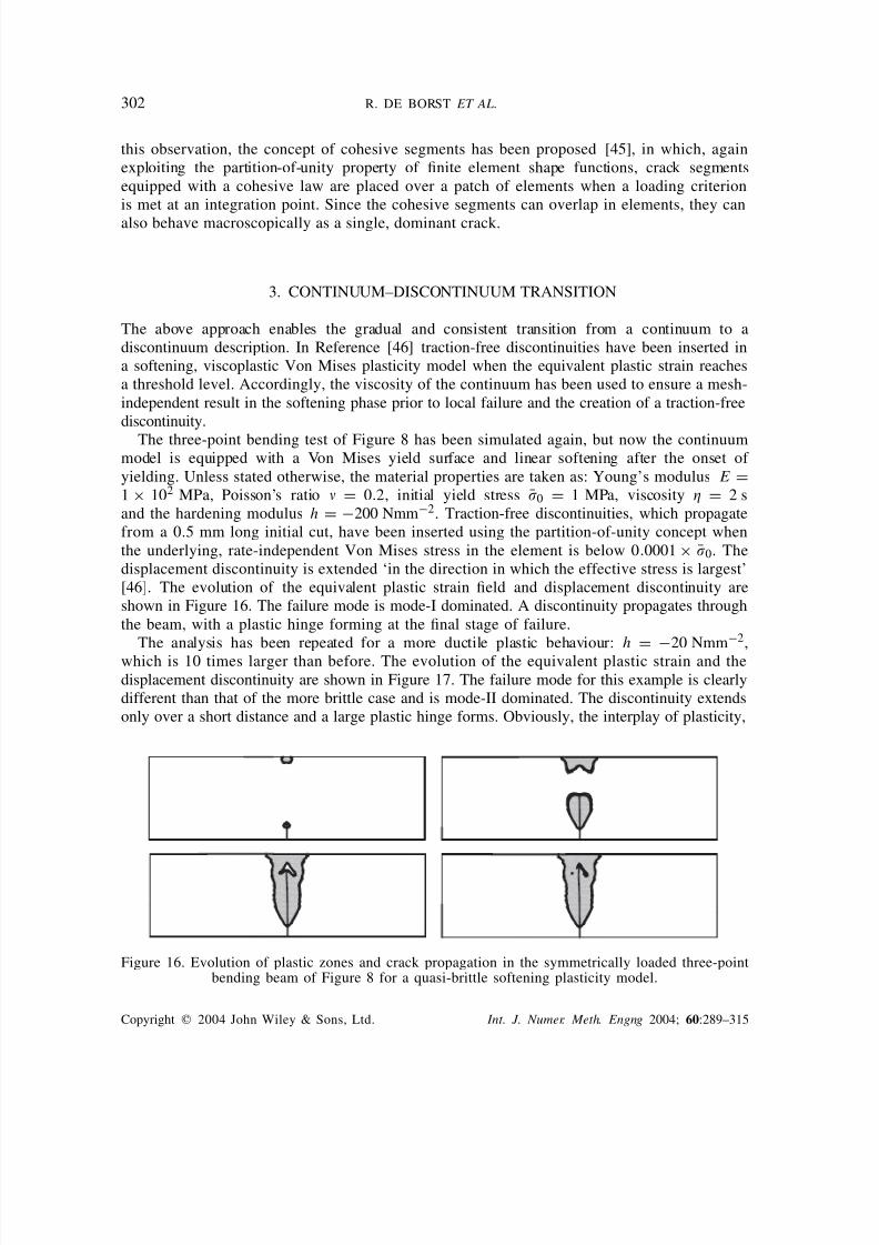
The three-point bending test of Figure 8 has been simulated again, but now the continuummodel is equipped with a Von Mises yield surface and linear softening after the onset of
yielding. Unless stated otherwise, the material properties are taken as: Young’s modulus E =
1 × 10² MPa, Poisson’s ratio = 0.2, initial yield stress 0 = 1 MPa, viscosity = 2 s
and the hardening modulus h = −200 Nmm−2. Traction-free discontinuities, which propagate
from a 0.5 mm long initial cut, have been inserted using the partition-of-unity concept when
the underlying, rate-independent Von Mises stress in the element is below 0.0001 × 0. The
displacement discontinuity is extended ‘in the direction in which the effective stress is largest’
[46]. The evolution of the equivalent plastic strain field and displacement discontinuity are
shown in Figure 16. The failure mode is mode-I dominated. A discontinuity propagates through
the beam, with a plastic hinge forming at the final stage of failure.
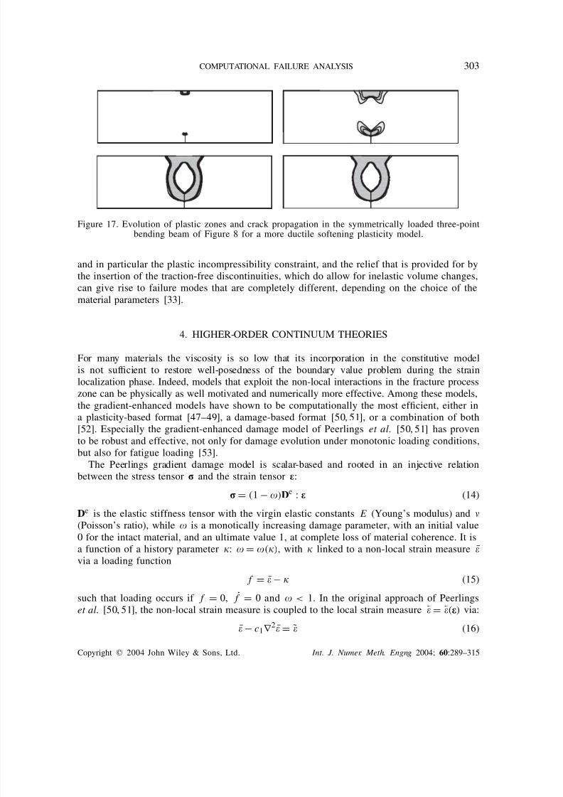
The analysis has been repeated for a more ductile plastic behaviour: h = −20 Nmm−2,
which is 10 times larger than before. The evolution of the equivalent plastic strain and the
displacement discontinuity are shown in Figure 17. The failure mode for this example is clearly
different than that of the more brittle case and is mode-II dominated. The discontinuity extends
only over a short distance and a large plastic hinge forms. Obviously, the interplay of plasticity,
Figure 16. Evolution of plastic zones and crack propagation in the symmetrically loaded three-pointbending beam of Figure 8 for a quasi-brittle softening plasticity model.
Copyright 2004 John Wiley & Sons, Ltd. Int. J. Numer. Meth. Engng 2004; 60:289–315
8/11/2019 Cohesive Zone Model-ref
http://slidepdf.com/reader/full/cohesive-zone-model-ref 15/27
COMPUTATIONAL FAILURE ANALYSIS 303
Figure 17. Evolution of plastic zones and crack propagation in the symmetrically loaded three-pointbending beam of Figure 8 for a more ductile softening plasticity model.
and in particular the plastic incompressibility constraint, and the relief that is provided for by
the insertion of the traction-free discontinuities, which do allow for inelastic volume changes,can give rise to failure modes that are completely different, depending on the choice of the
material parameters [33].
4. HIGHER-ORDER CONTINUUM THEORIES
For many materials the viscosity is so low that its incorporation in the constitutive model
is not sufficient to restore well-posedness of the boundary value problem during the strain
localization phase. Indeed, models that exploit the non-local interactions in the fracture process
zone can be physically as well motivated and numerically more effective. Among these models,
the gradient-enhanced models have shown to be computationally the most efficient, either in
a plasticity-based format [47–49], a damage-based format [50, 51], or a combination of both[52]. Especially the gradient-enhanced damage model of Peerlings et al. [50, 51] has proven
to be robust and effective, not only for damage evolution under monotonic loading conditions,
but also for fatigue loading [53].
The Peerlings gradient damage model is scalar-based and rooted in an injective relation
between the stress tensor and the strain tensor :
= (1 − )De : (14)
De is the elastic stiffness tensor with the virgin elastic constants E (Young’s modulus) and
(Poisson’s ratio), while is a monotically increasing damage parameter, with an initial value
0 for the intact material, and an ultimate value 1, at complete loss of material coherence. It is
a function of a history parameter : = (), with linked to a non-local strain measure
via a loading function
f = − (15)
such that loading occurs if f = 0, f = 0 and < 1. In the original approach of Peerlings
et al. [50, 51], the non-local strain measure is coupled to the local strain measure = () via:
− c1∇ 2 = (16)
Copyright 2004 John Wiley & Sons, Ltd. Int. J. Numer. Meth. Engng 2004; 60:289–315

8/11/2019 Cohesive Zone Model-ref
http://slidepdf.com/reader/full/cohesive-zone-model-ref 16/27
8/11/2019 Cohesive Zone Model-ref
http://slidepdf.com/reader/full/cohesive-zone-model-ref 17/27
COMPUTATIONAL FAILURE ANALYSIS 305
u
A =10 mm A = 9 mm
45 mm45 mm 10 mm
2 2
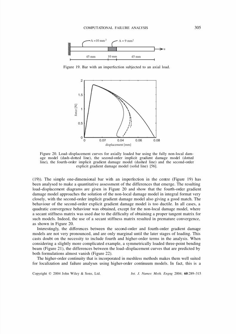
Figure 19. Bar with an imperfection subjected to an axial load.
0 0.02 0.04 0.06 0.08
displacement [mm]
0
0.5
1
1.5
2
f o r c e [ N ]
Figure 20. Load–displacement curves for axially loaded bar using the fully non-local dam-age model (dash–dotted line), the second-order implicit gradient damage model (dottedline), the fourth-order implicit gradient damage model (dashed line) and the second-order
explicit gradient damage model (solid line) [56].
(19)). The simple one-dimensional bar with an imperfection in the centre (Figure 19) has
been analysed to make a quantitative assessment of the differences that emerge. The resulting
load–displacement diagrams are given in Figure 20 and show that the fourth-order gradient
damage model approaches the solution of the non-local damage model in integral format very
closely, with the second-order implicit gradient damage model also giving a good match. The
behaviour of the second-order explicit gradient damage model is too ductile. In all cases, a
quadratic convergence behaviour was obtained, except for the non-local damage model, where
a secant stiffness matrix was used due to the difficulty of obtaining a proper tangent matrix for
such models. Indeed, the use of a secant stiffness matrix resulted in premature convergence,
as shown in Figure 20.
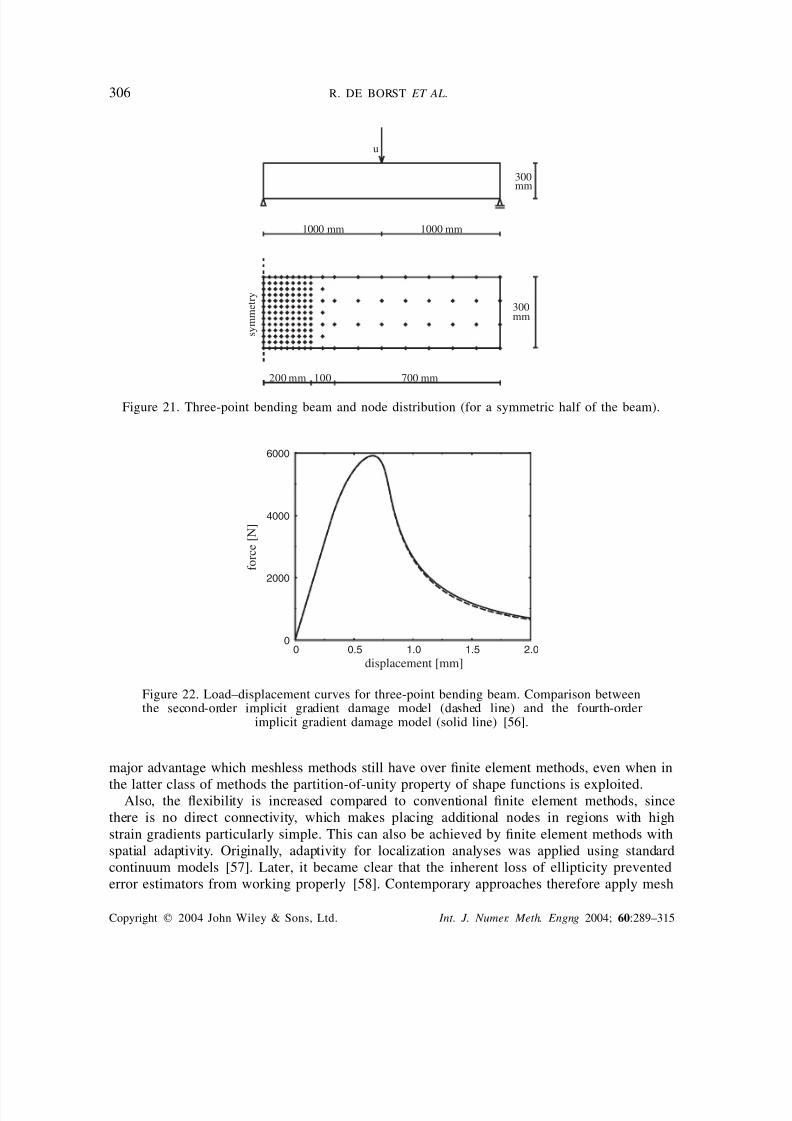
Interestingly, the differences between the second-order and fourth-order gradient damage
models are not very pronounced, and are only marginal until the later stages of loading. Thiscasts doubt on the necessity to include fourth and higher-order terms in the analysis. When
considering a slightly more complicated example, a symmetrically loaded three-point bending
beam (Figure 21), the differences between the load–displacement curves that are predicted by
both formulations almost vanish (Figure 22).
The higher-order continuity that is incorporated in meshless methods makes them well suited
for localization and failure analyses using higher-order continuum models. In fact, this is a
Copyright 2004 John Wiley & Sons, Ltd. Int. J. Numer. Meth. Engng 2004; 60:289–315
8/11/2019 Cohesive Zone Model-ref
http://slidepdf.com/reader/full/cohesive-zone-model-ref 18/27
306 R. DE BORST ET AL.
u
200 mm 100
mm300
700 mm
mm
1000 mm
300
1000 mm
s y m m e t r y
Figure 21. Three-point bending beam and node distribution (for a symmetric half of the beam).
0 0.5 1.0 1.5 2.0
displacement [mm]
0
2000
4000
6000
f o r c e [ N ]
Figure 22. Load–displacement curves for three-point bending beam. Comparison betweenthe second-order implicit gradient damage model (dashed line) and the fourth-order
implicit gradient damage model (solid line) [56].
major advantage which meshless methods still have over finite element methods, even when in
the latter class of methods the partition-of-unity property of shape functions is exploited.Also, the flexibility is increased compared to conventional finite element methods, since
there is no direct connectivity, which makes placing additional nodes in regions with high
strain gradients particularly simple. This can also be achieved by finite element methods with
spatial adaptivity. Originally, adaptivity for localization analyses was applied using standard
continuum models [57]. Later, it became clear that the inherent loss of ellipticity prevented
error estimators from working properly [58]. Contemporary approaches therefore apply mesh
Copyright 2004 John Wiley & Sons, Ltd. Int. J. Numer. Meth. Engng 2004; 60:289–315

8/11/2019 Cohesive Zone Model-ref
http://slidepdf.com/reader/full/cohesive-zone-model-ref 19/27
COMPUTATIONAL FAILURE ANALYSIS 307
adaptivity techniques for failure analyses in conjunction with cohesive-zone models or with
regularized continuum models [58–60]. Similarly, the discretization itself cannot provide a
regularization, neither for finite element methods, nor for meshless methods. Indeed, for the
latter class of methods the nodal spacing directly relates to the width of the localization zone
that is resolved if no regularization is provided for the continuum model.
6. RELIABILITY METHODS
So far, the discussion has concentrated on localization and the ensuing failure in solids which
have uniform strength and stiffness properties. In reality, strength and stiffness have a random
distribution over any structure. The distribution and the size of imperfections may have a
profound influence on the localization pattern and, therefore, on the ultimate failure load, as
was demonstrated more than half a century ago by Koiter in his landmark dissertation [61] on
the influence of imperfections in elastic solids. We may expect that this observation holds a
fortiori if material degradation plays a role.
Thus, for realistic analyses of localization and failure, material parameters like Young’s
modulus, the tensile strength and the fracture energy should be considered as random fields,
and the most probable realization(s) should be sought which lead to failure or violate a certain
serviceability criterion. Indeed, in such analyses, not only the scatter in material parameters,
but also the uncertainty in the boundary conditions should be considered. The simplest, but
also the most expensive method, would be to start a non-linear analysis from different random
distributions and to obtain the statistics of the response by carrying out a sufficient number
of such Monte-Carlo simulations [62]. Evidently, this is very expensive and a more versatile
approach is to use the finite element reliability method [63–65].
The latter approach formally departs from a coupling between the random field of mate-
rial parameters (and/or boundary conditions) and the equilibrium path of the body. Through
appropriate discretization techniques [66], the random fields can be discretized into a set of
uncorrelated standard normal variables that will be denoted as S. The simplest example of this
kind of discretization is given by the midpoint method, in which the domain of the random
field is discretized into a set of finite element-like cells r. The random field, particularized at
the centroid xc of each cell, provides a set of correlated random variables V. These variables
are then converted into the set S of uncorrelated standard normally distributed variables through
Nataf’s transformation [67]. The geometrical interpretation of this discretization is provided in
Figure 23. The cells r do not need to coincide with the finite element discretization. However,
the computer implementation is facilitated by choosing r coinciding with patches of finite
elements (Figure 24).
The equilibrium path of the considered body is related to the random variables S through
a non-linear finite element algorithm. The statistical properties of any measure Q of theequilibrium path, like the peak load or the energy consumption, can then be studied in the
standard normal space expanded by S. In particular, the cumulative distribution of Q evaluated
at the realization q0 is expressed as
F Q(q0) =
q(s)<q0
d(s) (20)
Copyright 2004 John Wiley & Sons, Ltd. Int. J. Numer. Meth. Engng 2004; 60:289–315

8/11/2019 Cohesive Zone Model-ref
http://slidepdf.com/reader/full/cohesive-zone-model-ref 20/27
308 R. DE BORST ET AL.
Finite element discretisationΩr
Figure 23. Schematic representation of the mid-point discretization technique for random fields.
Figure 24. Selection of the domains r inrelation to the finite element mesh.
Figure 25. Schematization of the evaluation of the cumulative distribution of Q in the Q space (left)and in the uncorrelated standard normal space S (right).
where d(s) represents the uncorrelated standard normal probability measure. This is also
schematized in Figure 25. The exact evaluation of the integral in the right hand side of Equation (20) is still too expensive from a computational point of view. Alternatively, the
surface q(s) = q0 is approximated by a first-order or second-order surface. The most convenient
point for approximation is given by the closest point to the origin on surface q(s) = q0. This
point, which represents the realization of S with the largest probability density, is referred to as
design point or -point and represented by s. In the particular case that the surface q(s) = q0has been approximated by a hyperplane, the cumulative distribution of Q at q0 is approximated
Copyright 2004 John Wiley & Sons, Ltd. Int. J. Numer. Meth. Engng 2004; 60:289–315
8/11/2019 Cohesive Zone Model-ref
http://slidepdf.com/reader/full/cohesive-zone-model-ref 21/27
COMPUTATIONAL FAILURE ANALYSIS 309
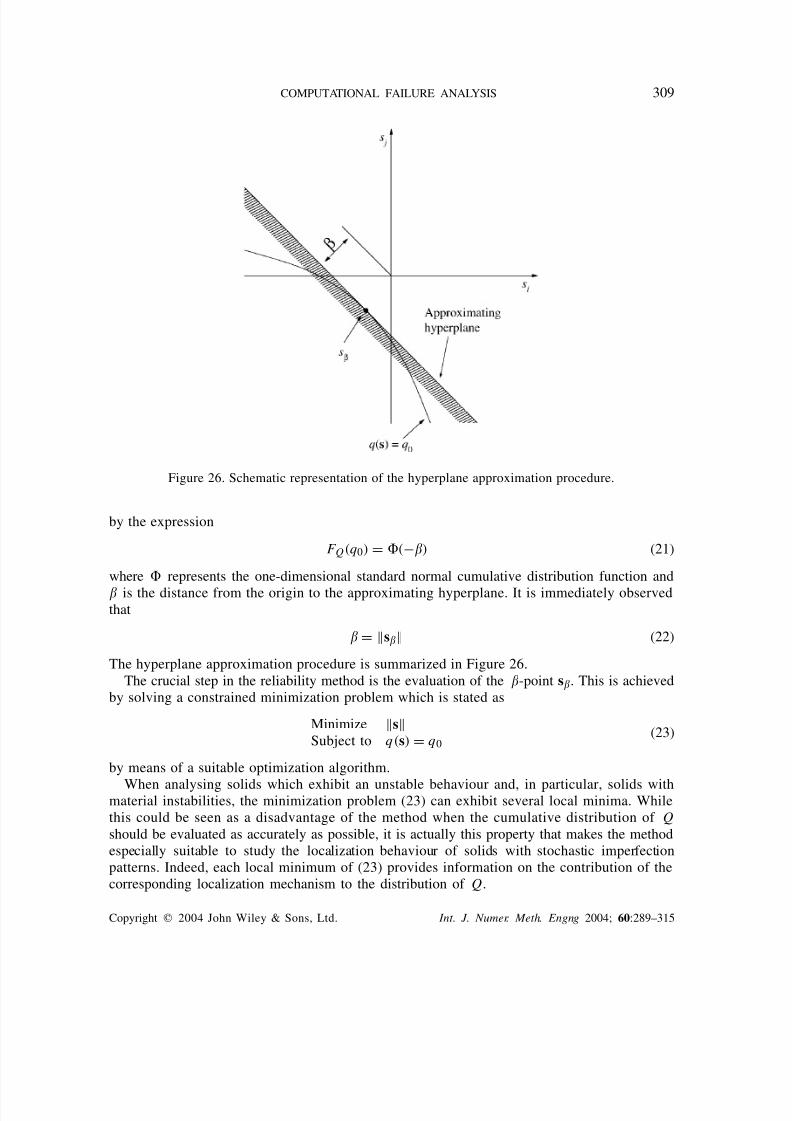
Figure 26. Schematic representation of the hyperplane approximation procedure.
by the expression
F Q(q0) = (−) (21)
where represents the one-dimensional standard normal cumulative distribution function and
is the distance from the origin to the approximating hyperplane. It is immediately observedthat
= s (22)
The hyperplane approximation procedure is summarized in Figure 26.
The crucial step in the reliability method is the evaluation of the -point s. This is achieved
by solving a constrained minimization problem which is stated as
Minimize s
Subject to q(s) = q0(23)
by means of a suitable optimization algorithm.
When analysing solids which exhibit an unstable behaviour and, in particular, solids withmaterial instabilities, the minimization problem (23) can exhibit several local minima. While
this could be seen as a disadvantage of the method when the cumulative distribution of Q
should be evaluated as accurately as possible, it is actually this property that makes the method
especially suitable to study the localization behaviour of solids with stochastic imperfection
patterns. Indeed, each local minimum of (23) provides information on the contribution of the
corresponding localization mechanism to the distribution of Q.
Copyright 2004 John Wiley & Sons, Ltd. Int. J. Numer. Meth. Engng 2004; 60:289–315

8/11/2019 Cohesive Zone Model-ref
http://slidepdf.com/reader/full/cohesive-zone-model-ref 22/27
310 R. DE BORST ET AL.
Figure 27. Schematic representation of a tensile test on a double-edge-notchedspecimen. Dimensions in mm.
As an example a double-edge-notched specimen is considered (Figure 27). For detailed
information regarding the parameters that have been used and the way in which the analysis
has been carried out, the reader is referred to References [63, 65]. The considered characteristicproperty Q of the equilibrium path is the peak load. The cumulative distribution function of
Q can then be associated with the probability of failure, since it represents the probability that
the peak load is lower than a given threshold.
Tensile tests on such specimens tend to be sensitive to the boundary conditions, in particular
when the brittleness of the material increases. When an imperfection is not imposed in the
material, nor an asymmetry in the boundary conditions, the deformations will remain symmetric
throughout the entire equilibrium path. However, if either of these occurs, asymmetric crack
propagation evolves from one of the notches at a generic stage in the loading process. The
probability that either of these failure modes occurs can be simulated via the approach discussed
above where the tensile strength is randomized, while starting the solution algorithm from a
symmetric as well as from an asymmetric realization. In particular, the influence of the boundary
conditions can be quantified. For instance, taking the upper loading platen of the double-edge-notched specimen fixed, the probability of failure was found to be P s = 5.84×10⁻², irrespective
whether the algorithm was started from a symmetric or from an asymmetric realization. Indeed,
the failure mode was purely symmetric. However, when the upper loading platen is allowed to
rotate freely, an asymmetric mode was found with a probability of failure that is significantly
higher than that of the symmetric model, namely P a = 0.41. The symmetric and the asymmetric
modes are represented in Figure 28. Next, the analysis was repeated for a longer specimen
Copyright 2004 John Wiley & Sons, Ltd. Int. J. Numer. Meth. Engng 2004; 60:289–315
8/11/2019 Cohesive Zone Model-ref
http://slidepdf.com/reader/full/cohesive-zone-model-ref 23/27
COMPUTATIONAL FAILURE ANALYSIS 311
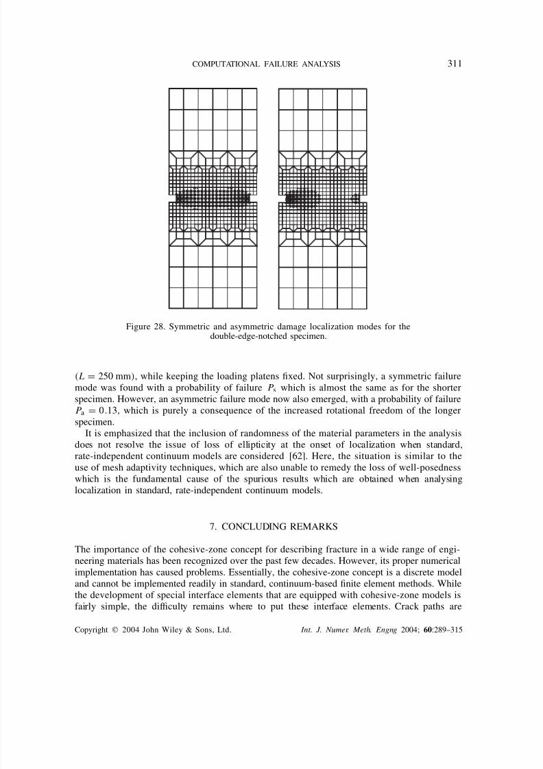
Figure 28. Symmetric and asymmetric damage localization modes for thedouble-edge-notched specimen.
(L = 250 mm), while keeping the loading platens fixed. Not surprisingly, a symmetric failure
mode was found with a probability of failure P s which is almost the same as for the shorter
specimen. However, an asymmetric failure mode now also emerged, with a probability of failure
P a = 0.13, which is purely a consequence of the increased rotational freedom of the longer
specimen.
It is emphasized that the inclusion of randomness of the material parameters in the analysis
does not resolve the issue of loss of ellipticity at the onset of localization when standard,
rate-independent continuum models are considered [62]. Here, the situation is similar to the
use of mesh adaptivity techniques, which are also unable to remedy the loss of well-posedness
which is the fundamental cause of the spurious results which are obtained when analysing
localization in standard, rate-independent continuum models.
7. CONCLUDING REMARKS
The importance of the cohesive-zone concept for describing fracture in a wide range of engi-
neering materials has been recognized over the past few decades. However, its proper numerical
implementation has caused problems. Essentially, the cohesive-zone concept is a discrete model
and cannot be implemented readily in standard, continuum-based finite element methods. While
the development of special interface elements that are equipped with cohesive-zone models is
fairly simple, the difficulty remains where to put these interface elements. Crack paths are
Copyright 2004 John Wiley & Sons, Ltd. Int. J. Numer. Meth. Engng 2004; 60:289–315

8/11/2019 Cohesive Zone Model-ref
http://slidepdf.com/reader/full/cohesive-zone-model-ref 24/27
312 R. DE BORST ET AL.
normally not known in advance. To partly circumvent this difficulty, proposals have been
made to insert interface elements between all continuum elements, to carry out remeshing
procedures or to use mesh-free methods. Neither of these approaches is entirely satisfactory
and it seems that only recently, namely by using the partition-of-unity property of finite el-
ement shape functions an elegant and powerful method has been developed to fully exploitthe potential of cohesive-zone models for arbitrary crack propagation. A consistent extension
to dynamics is possible as well as a transparent extension to multiphasic media. Among the
added benefits we list the ability to model delaminations independent of the underlying mesh
structure, to achieve a consistent formulation for large strains and to obtain a smooth transi-
tion from a plastifying or damaging continuum to a traction-free, macroscopically observable
crack.
With the exploitation of the partition-of-unity property of finite element shape functions,
mesh-free methods have lost much of their attractiveness. However, they still retain the benefit
of higher-order continuity, which can be exploited when quantifying the effect of higher-order
gradients which occur in gradient-enhanced damage or plasticity models for the description of
softening in solids.
As a final point, it is emphasized that materials and structures are never homogeneous.
Imperfections play an important role in triggering failure modes. For this reason a method has
been discussed that can quantify the effect of the size and the location of imperfections in
softening solids.
REFERENCES
1. Babuska I, Melenk JM. The partition of unity method. International Journal for Numerical Methods in
Engineering 1997; 40:727–758.
2. Belytschko T, Lu YY, Gu L. Element-free Galerkin methods. International Journal for Numerical Methods
in Engineering 1994; 37:229–256.3. Barenblatt GI. The mathematical theory of equilibrium cracks in brittle fracture. Advances in Applied
Mechanics 1962; 7:55–129.
4. Dugdale DS. Yielding of steel sheets containing slits. Journal of the Mechanics and Physics of Solids 1960;
8:100–108.
5. Hillerborg A, Modeer M, Petersson PE. Analysis of crack formation and crack growth in concrete by means
of fracture mechanics and finite elements. Cement and Concrete Research 1976; 6:773–782.
6. Tvergaard V, Hutchinson JW. The relation between crack growth resistance and fracture process parameters
in elastic-plastic solids. Journal of the Mechanics and Physics of Solids 1992; 40:1377–1397.
7. Reinhardt HW, Cornelissen HAW. Post-peak cyclic behaviour of concrete in uniaxial and alternating tensile
and compressive loading. Cement and Concrete Research 1984; 14:263–270.
8. Hutchinson JW, Evans AG. Mechanics of materials: top-down approaches to fracture. Acta Materialia 2000;
48:125–135.
9. Rots JG. Strain-softening analysis of concrete fracture specimens. In Fracture Toughness and Fracture Energyof Concrete, Wittmann FH (ed.). Elsevier Science Publishers: Amsterdam, The Netherlands, 1986; 137–148.
10. Chandra N, Li H, Shet C, Ghonem H. Some issues in the application of cohesive zone models for
metal–ceramic interfaces. International Journal of Solids and Structures 2002; 39:2827–2855.
11. Arrea M, Ingraffea AR. Mixed-mode crack propagation in mortar and concrete. Report 81-13. Cornell
University, Ithaca, New York, 1982.
12. Rots JG. Smeared and discrete representations of localized fracture. International Journal of Fracture 1991;
51:45–59.
Copyright 2004 John Wiley & Sons, Ltd. Int. J. Numer. Meth. Engng 2004; 60:289–315

8/11/2019 Cohesive Zone Model-ref
http://slidepdf.com/reader/full/cohesive-zone-model-ref 25/27
COMPUTATIONAL FAILURE ANALYSIS 313
13. Schellekens JCJ, de Borst R. On the numerical integration of interface elements. International Journal for
Numerical Methods in Engineering 1992; 36:43–66.14. Schellekens JCJ, de Borst R. A non-linear finite element approach for the analysis of mode-I free edge
delamination in composites. International Journal of Solids and Structures 1993; 30:1239–1253.15. Schellekens JCJ, de Borst R. Free edge delamination in carbon-epoxy laminates: a novel numerical/
experimental approach. Composite Structures 1994; 28:357–373.16. Allix O, Ladevèze P. Interlaminar interface modelling for the prediction of delamination. Composite Structures
1992; 22:235–242.17. Allix O, Corigliano A. Geometrical and interfacial non-linearities in the analysis of delamination in composites.
International Journal of Solids and Structures 1999; 36:2189–2216.18. Xu XP, Needleman A. Numerical simulations of fast crack growth in brittle solids. Journal of the Mechanics
and Physics of Solids 1994; 42:1397–1434.19. Camacho GT, Ortiz M. Computational modeling of impact damage in brittle materials. International Journal
of Solids and Structures 1996; 33:2899–2938.20. Tijssens MGA, van der Giessen E, Sluys LJ. Modeling of crazing using a cohesive surface methodology.
Mechanics of Materials 2000; 32:19–35.21. Tijssens MGA, Sluys LJ, van der Giessen E. Numerical simulation of quasi-brittle fracture using damaging
cohesive surfaces. European Journal of Mechanics – A/Solids 2000; 19:761–779.22. Pietruszczak S, Mróz Z. Finite element analysis of deformation of strain softening materials. International
Journal for Numerical Methods in Engineering 1981; 17:327–334.23. Bažant ZP, Oh B. Crack band theory for fracture of concrete. RILEM Materials and Structures 1983; 16:
155–177.24. de Borst R. Computation of post-bifurcation and post-failure behaviour of strain-softening solids. Computers
and Structures 1987; 25:211–224.25. Feenstra PH, de Borst R. A plasticity model for mode-I cracking in concrete. International Journal for
Numerical Methods in Engineering 1995; 38:2509–2529.26. Simo JC, Oliver J, Armero F. An analysis of strong discontinuities induced by softening relations in
rate-independent solids. Computational Mechanics 1993; 12:277–296.27. Larsson R, Runesson K, Ottosen NS. Discontinuous displacement approximation for capturing plastic
localization. International Journal for Numerical Methods in Engineering 1993; 36:2087–2105.28. Lotfi HR, Shing PB. Embedded representation of fracture in concrete with mixed elements. International
Journal for Numerical Methods in Engineering 1995; 38:1307–1325.29. Ortiz M, Leroy Y, Needleman A. A finite element method for localized failure analysis. Computer Methods
in Applied Mechanics and Engineering 1987; 61
:189–214.30. Belytschko T, Fish J, Engelman BE. A finite element with embedded localization zones. Computer Methods
in Applied Mechanics and Engineering 1988; 70:59–89.31. Sluys LJ, Berends AH. Discontinuous failure analysis for mode-I and mode-II localization problems.
International Journal of Solids and Structures 1998; 35:4257–4274.32. de Borst R, Wells GN, Sluys LJ. Some observations on embedded discontinuity models. Engineering
Computations 2001; 18:241–254.33. Wells GN. Discontinuous Modelling of Strain Localization and Failure. Dissertation, Delft University of
Technology, Delft, 2001.34. Mosler J, Meschke G. A comparison of embedded discontinuity approaches with fracture energy based
smeared crack models. In Proceedings of the Fifth Congress on Computational Mechanics (WCCM V ). Mang
HA, Rammerstorfer FG, Eberhardsteiner J (eds). Vienna University of Technology: Vienna, Austria, 2002
(Paper 81054).35. de Borst R, Nauta P. Non-orthogonal cracks in a smeared finite element model. Engineering Computations
1985; 2:35–46.
36. Belytschko T, Black T. Elastic crack growth in finite elements with minimal remeshing. International Journal for Numerical Methods in Engineering 1999; 45:601–620.
37. Moës N, Dolbow J, Belytschko T. A finite element method for crack growth without remeshing. International
Journal for Numerical Methods in Engineering 1999; 46:131–150.38. Wells GN, Sluys LJ. A new method for modeling cohesive cracks using finite elements. International Journal
for Numerical Methods in Engineering 2001; 50:2667–2682.39. Wells GN, de Borst R, Sluys LJ. A consistent geometrically non-linear approach for delamination.
International Journal for Numerical Methods in Engineering 2002; 54:1333–1355.
Copyright 2004 John Wiley & Sons, Ltd. Int. J. Numer. Meth. Engng 2004; 60:289–315

8/11/2019 Cohesive Zone Model-ref
http://slidepdf.com/reader/full/cohesive-zone-model-ref 26/27
314 R. DE BORST ET AL.
40. Hughes TJR. Multiscale phenomena: Green’s functions, the Dirichlet-to-Neumann formulation, subgrid scale
models, bubbles and the origins of stabilized methods. Computer Methods in Applied Mechanics and
Engineering 1995; 127:387–401.41. Gravouil A, Moës N, Belytschko T. Non-planar 3D crack growth by the extended finite element and level
sets—Part 1: mechanical model. International Journal for Numerical Methods in Engineering 2002; 53:
2549–2568.42. Gravouil A, Moës N, Belytschko T. Non-planar 3D crack growth by the extended finite element and
level sets—Part 2: level set update. International Journal for Numerical Methods in Engineering 2002; 53:
2569–2586.43. Remmers JJC, Wells GN, de Borst R. A solid-like shell element allowing for arbitrary delaminations.
International Journal for Numerical Methods in Engineering 2003; 58:2013–2040.44. Parisch H. A continuum-based shell theory for non-linear applications. International Journal for Numerical
Methods in Engineering 1995; 38:1855–1883.45. Remmers JJC, de Borst R, Needleman A. A cohesive segments method for the simulation of crack growth.
Computational Mechanics 2003; 31:69–77.46. Wells GN, Sluys LJ, de Borst R. Simulating the propagation of displacement discontinuities in a
regularized strain-softening medium. International Journal for Numerical Methods in Engineering 2002; 53:
1235–1256.47. de Borst R, Mühlhaus HB. Gradient-dependent plasticity: formulation and algorithmic aspects. International
Journal for Numerical Methods in Engineering 1992; 35:521–539.48. de Borst R, Pamin J. Some novel developments in finite element procedures for gradient-dependent plasticity.
International Journal for Numerical Methods in Engineering 1996; 39:2477–2505.49. Fleck NA, Hutchinson JW. A phenomenological theory for strain gradient effects in plasticity. Journal of
the Mechanics and Physics of Solids 1993; 41:1825–1857.50. Peerlings RHJ, de Borst R, Brekelmans WAM, de Vree HPJ. Gradient-enhanced damage for quasi-brittle
materials. International Journal for Numerical Methods in Engineering 1996; 39:3391–3403.51. Peerlings RHJ, de Borst R, Brekelmans WAM, Geers MGD. Localization issues in local and non-local
continuum approaches to fracture. European Journal of Mechanics – A/Solids 2002; 21:175–189.52. de Borst R, Pamin J, Geers MGD. On coupled gradient-dependent plasticity and damage theories with a
view to localization analysis. European Journal of Mechanics – A/Solids 1999; 18:939–962.53. Peerlings RHJ, Brekelmans WAM, de Borst R, Geers MGD. Gradient-enhanced damage modelling of high-
cycle fatigue. International Journal for Numerical Methods in Engineering 2000; 49:1547–1569.54. Pijaudier-Cabot G, Bažant ZP. Nonlocal damage theory. Journal of Engineering Mechanics (ASCE) 1987;
113:1512–1533.55. Peerlings RHJ, de Borst R, Brekelmans WAM, Geers MGD. Gradient-enhanced damage modelling of concrete
fracture. Mechanics of Cohesive-frictional Materials 1998; 3:323–342.56. Askes H, Pamin P, de Borst R. Dispersion analysis and element-free Galerkin solutions of second and
fourth-order gradient-enhanced damage models. International Journal for Numerical Methods in Engineering
2000; 49:811–832.57. Zienkiewicz OC, Huang GC. A note on localization phenomena and adaptive finite element analysis in
forming processes. Communications in Applied Numerical Methods 1990; 6:71–76.58. Peric D, Yu JG, Owen DRJ. On error estimates and adaptivity in elastoplastic solids: Applications to
the numerical simulation of strain localization in classical and Cosserat continua. International Journal for
Numerical Methods in Engineering 1994; 37:1351–1379.59. Lackner R, Mang HA. Adaptivity in computational mechanics of concrete structures. International Journal
for Numerical and Analytical Methods in Geomechanics 2001; 25:711–739.60. Askes H, Sluys LJ. Remeshing strategies for adaptive ALE analysis of strain localization. European Journal
of Mechanics – A/Solids 2000; 19:447–467.
61. Koiter WT. Over de Stabiliteit van het Elastisch Evenwicht. Dissertation. Delft University of Technology,Delft, 1945.
62. Carmeliet J, de Borst R. Stochastic approaches for damage evolution in standard and non-standard continua.
International Journal of Solids and Structures 1995; 32:1149–1160.63. Gutiérrez MA, de Borst R. Deterministic and stochastic analysis of size effects and damage evolution in
quasi-brittle materials. Archive of Applied Mechanics 1999; 69:655–676.64. Gutiérrez MA, de Borst R. Stochastic aspects of localised failure: material and boundary imperfections.
International Journal of Solids and Structures 2000; 37:7145–7159.
Copyright 2004 John Wiley & Sons, Ltd. Int. J. Numer. Meth. Engng 2004; 60:289–315
8/11/2019 Cohesive Zone Model-ref
http://slidepdf.com/reader/full/cohesive-zone-model-ref 27/27
COMPUTATIONAL FAILURE ANALYSIS 315
65. Gutiérrez MA. Objective Simulation of Failure in Heterogeneous Softening Solids. Dissertation. Delft
University of Technology, Delft, 1999.
66. Li CC, Der Kiureghian A. Optimal discretization of random fields. Journal of Engineering Mechanics (ASCE)
1993; 119:1136–1154.
67. Der Kiureghian A, Liu PL. Structural reliability under incomplete probability information. Journal of Engineering Mechanics (ASCE) 1986; 112:85–104.
Copyright 2004 John Wiley & Sons, Ltd. Int. J. Numer. Meth. Engng 2004; 60:289–315