Coherent State Path Integral Quantization of Quantum Field...

8

Coherent State Path Integral Quantization ofQuantum Field Theory

8.1 Coherent states and path integral quantization.

8.1.1 Coherent States

Let us consider a Hilbert space spanned by a complete set of harmonicoscillator states |n⟩, with n = 0, . . . ,∞. Let a† and a be a pair of creationand annihilation operators acting on that Hilbert space, and satisfying thecommutation relations

[a, a†

]= 1 ,

[a†, a†

]= 0 , [a, a] = 0 (8.1)

These operators generate the harmonic oscillators states |n⟩ in the usualway,

|n⟩ = 1√n!

(a†)n

|0⟩, a|0⟩ = 0 (8.2)

where |0⟩ is the vacuum state of the oscillator.Let us denote by |z⟩ the coherent state

|z⟩ = eza†|0⟩, ⟨z| = ⟨0| eza (8.3)

where z is an arbitrary complex number and z is the complex conjugate.The coherent state |z⟩ has the defining property of being a wave packet withoptimal spread, i.e., the Heisenberg uncertainty inequality is an equality forthese coherent states.

How does a act on the coherent state |z⟩?

a|z⟩ =∞∑

n=0

zn

n!a(a†)n

|0⟩ (8.4)

Since [a,(a†)n]

= n(a†)n−1

(8.5)

8.1 Coherent states and path integral quantization. 219

we get

a|z⟩ =∞∑

n=0

zn

n!

([a,(a†)n]

+(a†)n

a)

|0⟩ (8.6)

Thus, we find

a|z⟩ =∞∑

n=0

zn

n!n(a†)n−1

|0⟩ ≡ z |z⟩ (8.7)

Therefore |z⟩ is a right eigenvector of a and z is the (right) eigenvalue.Likewise we get

a†|z⟩ =a†∞∑

n=0

zn

n!

(a†)n

|0⟩

=∞∑

n=0

zn

n!

(a†)n+1

|0⟩

=∞∑

n=0

(n + 1)zn

(n+ 1)!

(a†)n+1

|0⟩

=∞∑

n=1

nzn−1

n!

(a†)n

|0⟩ (8.8)

Thus,

a†|z⟩ = ∂

∂z|z⟩ (8.9)

Another quantity of interest is the overlap of two coherent states, ⟨z|z′⟩,

⟨z|z′⟩ = ⟨0|eza ez′a† |0⟩ (8.10)

We will calculate this matrix element using the Baker-Hausdorff formulas

eA eB = eA+ B +

1

2

[A, B

]

= e

[A, B

]

eB eA (8.11)

which holds provided the commutator[A, B

]is a c-number, i.e., it is pro-

portional to the identity operator. Since[a, a†

]= 1, we find

⟨z|z′⟩ = ezz′⟨0|ez

′a† eza|0⟩ (8.12)

But

eza |0⟩ = |0⟩, ⟨0| ez′a† = ⟨0| (8.13)

220 Coherent State Path Integral Quantization of Quantum Field Theory

Hence we get

⟨z|z′⟩ = ezz′

(8.14)

An arbitrary state |ψ⟩ of this Hilbert space can be expanded in the harmonicoscillator basis states |n⟩,

|ψ⟩ =∞∑

n=0

ψn√n!

|n⟩ =∞∑

n=0

ψn

n!

(a†)n

|0⟩ (8.15)

The projection of the state |ψ⟩ onto the coherent state |z⟩ is

⟨z|ψ⟩ =∞∑

n=0

ψn

n!⟨z|(a†)n

|0⟩ (8.16)

Since

⟨z| a† = z ⟨z| (8.17)

we find

⟨z|ψ⟩ =∞∑

n=0

ψn

n!zn ≡ ψ(z) (8.18)

Therefore the projection of |ψ⟩ onto |z⟩ is the anti-holomorphic (i.e., anti-analytic) function ψ(z). In other words, in this representation, the space ofstates |ψ⟩ are in one-to-one correspondence with the space of anti-analyticfunctions.

In summary, the coherent states |z⟩ satisfy the following properties

a|z⟩ = z|z⟩ ⟨z|a = ∂z⟨z|a†|z⟩ = ∂z|z⟩ ⟨z|a† = z⟨z|⟨z|ψ⟩ = ψ(z) ⟨ψ|z⟩ = ψ(z)

(8.19)

Next we will prove the resolution of identity

I =

∫dzdz

2πie−zz |z⟩⟨z| (8.20)

Let |ψ⟩ and |φ⟩ be two arbitrary states

|ψ⟩ =∞∑

n=0

ψn√n!, |n⟩|φ⟩ =

∞∑

n=0

φn√n!

|n⟩

such that their inner product is

⟨φ|ψ⟩ =∞∑

n=0

φnψn

n!(8.21)


Let us compute the matrix element of the operator I given in Eq.(8.20),

⟨φ|I |ψ⟩ =∑

m.n

φnψn

n!⟨n|I|m⟩ (8.22)

Thus we need to find

⟨n|I|m⟩ =∫

dzdz

2πie−|z|

2⟨n|z⟩⟨z|m⟩ (8.23)

Recall that the integration measure is defined to be given by

dzdz

2πi=

dRezdImz

π(8.24)

where

⟨n|z⟩ = 1√n!⟨0| (a)n |z⟩ = zn√

n!⟨0|z⟩ (8.25)

and

⟨z|m⟩ = 1√m!⟨z|(a†)m

|0⟩ = zm√m!⟨z|0⟩ (8.26)

Now, since |⟨0|z⟩|2 = 1, we get

⟨n|I |m⟩ =∫

dzdz

2πi

e−|z|2

√n!m!

znzm =

∫ ∞

0ρdρ

∫ 2π

0

dϕ

2π

e−ρ2

√n!m!

ρn+mei(n −m)ϕ

(8.27)Thus,

⟨n|I|m⟩ = δn,mn!

∫ ∞

0dx xne−x = ⟨n|m⟩ (8.28)

Hence, we have found that

⟨φ|I |ψ⟩ = ⟨φ|ψ⟩ (8.29)

for any pair of states |ψ⟩ and |φ⟩. Therefore I is the identity operator inthis Hilbert space. We conclude that the set of coherent states |z⟩ is anover-complete set of states.

Furthermore, since

⟨z|(a†)n

(a)m |z′⟩ = znz′m⟨z|z′⟩ = znz′mezz′

(8.30)

we conclude that the matrix elements in generic coherent states |z⟩ and |z′⟩of any arbitrary normal ordered operator of the form

A =∑

n,m

An,m

(a†)n

(a)m (8.31)


are equal to

⟨z|A|z′⟩ =(∑

n,m

An,mznz′m)ezz

′(8.32)

Therefore, if A(a, a†) is an arbitrary normal ordered operator (relative tothe state |0⟩), its matrix elements are given by

⟨z|A(a, a†)|z′⟩ = A(z, z′) ezz′

(8.33)

where A(z, z′) is a function of two complex variables z and z′ obtained fromA by the formal replacement

a↔ z′ , a† ↔ z (8.34)

For example, the matrix elements of the number operator N = a†a, whichmeasures the number of excitations, is

⟨z|N |z′⟩ = ⟨z|a†a|z′⟩ = zz′ ezz′

(8.35)

8.1.2 Path Integrals and Coherent States

We will want to compute the matrix elements of the evolution operator U ,

U = e−iT

!H(a†, a)

(8.36)

where H(a†, a) is a normal ordered operator and T = tf − ti is the totaltime lapse. Thus, if |i⟩ and |f⟩ denote two arbitrary initial and final states,we can write the matrix element of U as

⟨f |e−iT

!H(a†, a)

|i⟩ = limϵ→0,N→∞

⟨f |(1− i

ϵ

!H(a†, a)

)N|i⟩ (8.37)

However now, instead of inserting a complete set of states at each inter-mediate time tj (with j = 1, . . . , N), we will insert an over-complete set ofcoherent states |zj⟩ at each time tj through the insertion of the resolution


of the identity,

⟨f |(1− i

ϵ

!H(a†, a)

)N|i⟩ =

=

∫ ( N∏

j=1

dzjdzj2πi

)e

−N∑

j=1

|zj |2 [N−1∏

k=1

⟨zk+1|(1− i

ϵ

!H(a†, a)

)|zk⟩

]

×⟨f |(1− i

ϵ

!H(a†, a)

)|zN ⟩⟨z1|

(1− i

ϵ

!H(a†, a)

)|zi⟩

(8.38)

In the limit ϵ→ 0 these matrix elements become

⟨zk+1|(1− i

ϵ

!H(a†, a)

)|zk⟩ =⟨zk+1|zk⟩ − i

ϵ

!⟨zk+1|H(a†, a)|zk⟩

=⟨zk+1|zk⟩[1− i

ϵ

!H(zk+1, zk)

](8.39)

where H(zk+1, zk) is a function obtained from the normal ordered Hamilto-nian by performing the substitutions a† → zk+1 and a→ zk.

Hence, we can write the following expression for the matrix element of theevolution operator of the form

⟨f |e−iT

!H(a†, a)

|i⟩ =

= limϵ→0,N→∞

∫ ⎛

⎝N∏

j=1

dzjdzj2πi

⎞

⎠ e

−N∑

j=1

|zj |2

e

N−1∑

j=1

zj+1zj N−1∏

j=1

[1− i

ϵ

!H(zk+1, zk)

]

×⟨f |zN ⟩⟨z1|i⟩[1− i

ϵ

!

⟨f |H|zN ⟩⟨f |zN ⟩

] [1− i

ϵ

!

⟨z1|H|i⟩⟨z1|i⟩

](8.40)

By further expanding the initial and final states in coherent states

⟨f | =∫

dzfdzf2πi

e−|zf |2ψf (zf )⟨zf |

|i⟩ =∫

dzidzi2πi

e−|zi|2ψi(zi)|zi⟩ (8.41)


we find the result

⟨f |e−iT

!H(a†, a)

|i⟩ =

=

∫DzDz e

i

!

∫ tf

ti

dt

[!

2i(z∂tz − z∂tz)−H(z, z)

]

e

1

2(|zi|2 + |zf |2)

ψf (zf )ψi(zi)

(8.42)

This is the coherent-state form of the path integral. We can identify in thisexpression the Lagrangian L as the quantity

L =!

2i(z∂tz − z∂tz)−H(z, z) (8.43)

Notice that the Lagrangian in the coherent-state representation is first or-der in time derivatives. Because of this feature we are not guaranteed thatthe paths are necessarily differentiable. This property leads to all kinds ofsubtleties that for the most part we will ignore in what follows.

8.1.3 Path integral for a gas of non-relativistic bosons at finitetemperature.

The field theoretic description of a gas of (spinless) non-relativistic bosonsis given in terms of the creation and annihilation field operators φ†(x) andφ(x), which satisfy the equal time commutation relations (in d space dimen-sions)

[φ(x), φ†(y)

]= δd(x− y) (8.44)

Relative to the empty state |0⟩, i.e.,

φ(x)|0⟩ = 0 (8.45)

the normal ordered Hamiltonian (in the Grand canonical Ensemble) is

H =

∫ddx φ†(x)

[− !2

2m2 − µ+ V (x)

]φ(x)

+1

2

∫ddx

∫ddy φ†(x)φ†(y)U(x− y)φ(y)φ(x) (8.46)

where m is the mass of the bosons, µ is the chemical potential, V (x) is anexternal potential and U(x − y) is the interaction potential between pairsof bosons.

Following our discussion of the coherent state path integral we see that itis immediate to write down a path integral for a thermodynamically large


system of bosons. The boson coherent states are now labelled by a complex

field φ(x) and its complex conjugate φ(x).

|φ(x)⟩ = e

∫dx φ(x)φ(x)

|0⟩ (8.47)

which has the coherent state property of being a right eigenstate of the fieldoperator φ(x),

φ(x)|φ⟩ = φ(x)|φ⟩ (8.48)

as well as obeying the resolution of the identity in this space of states

I =

∫DφDφ∗e

−∫

dx |φ(x)|2|φ⟩⟨φ| (8.49)

The matrix element of the evolution operator of this system between anarbitrary initial state |i⟩ and an arbitrary final state |f⟩, separated by a timelapse T = tf − ti (not to be confused with the temperature!), now takes theform

⟨f |e− i

!HT

|i⟩ =∫

DφDφ exp

i

!

∫ tf

ti

dt

(∫ddx

!

i

[φ(x, t)∂tφ(x, t)− φ(x, t)∂tφ(x, t)

]−H[φ, φ]

)

× Ψf (φ(x, tf ))Ψi(φ(x, ti)) e

1

2

∫dx(|φ(x, tf )|2 + |φ(x, ti)|2)

(8.50)

where the functional H[φ, φ] is

H[φ, φ] =

∫ddx φ(x)

[− !2

2m2 − µ+ V (x)

]φ(x)

+1

2

∫ddx

∫ddy |φ(x)|2|φ(y)|2U(x− y)

(8.51)

It is also possible to write the action S in the less symmetric but simplerform (where dx ≡ dtdx)

S =

∫dx φ(x)

(i!∂t +

!2

2m

2+ µ− V (x)

)φ(x)

− 1

2

∫dx

∫dy |φ(x)|2|φ(y)|2U(x− y)

(8.52)


where U(x− y) = U(x− y)δ(tx − ty).Therefore the path integral for a system of non-relativistic bosons (with

chemical potential µ) has the same form os the path integral of the chargedscalar field we discussed before except that the action is first order in timederivatives. th fact that the field is complex follows from the requirementthat the number of bosons is a globally conserved quantity, which is why oneis allowed to introduce a chemical potential, i.e. to use the Grand CanonicalEnsemble in the first place.

This formulation is useful to study superfluid Helium and similar prob-lems. Suppose for instance that we want to compute the partition functionZ for this system of bosons at finite temperature T ,

Z = tre−βH (8.53)

where β = 1/T (in units where kB = 1). The coherent-state path integralrepresentation of the partition function is obtained by

1. restricting the initial and final states to be the same |i⟩ = |f⟩ and arbi-trary

2. summing over all possible states3. a Wick rotation to imaginary time t → −iτ , with the time-span T →−iβ! (i.e., Periodic Boundary Conditions in imaginary time)

The result is the (imaginary time) path integral

Z =

∫DφDφ e−SE(φ, φ) (8.54)

where SE is the Euclidean action

SE(φ, φ) =1

!

∫ β

0dτ

∫dx φ

[!∂τ − µ− !2

2m2 +V (x)

]φ

+1

2!

∫ β

0dτ

∫dx

∫dy U(x− y) |φ(x)|2|φ(y)|2

(8.55)

The fields φ(x) = φ(x, τ) satisfy Periodic Boundary Conditions (PBC’s) inimaginary time

φ(x, τ) = φ(x, τ + β!) (8.56)

This requirement suggests an expansion of the field φ(x) in Fourier modesof the form

φ(x, τ) =∞∑

n=−∞

eiωnτ φ(x,ωn) (8.57)

8.2 Fermion Coherent States 227

where the frequencies ωn (the Matsubara frequencies) must be chosen sothat φ obeys the required PBCs. We find

ωn =2π

β!n =

2πT

!n , n ∈ Z (8.58)

where n is an arbitrary integer.

8.2 Fermion Coherent States

In this section we will develop a formalism for fermions which follows closelywhat we have done for bosons while accounting for the anti-commutingnature of fermionic operators, i. e. the Pauli Principle.

Let c†i be a set of fermion creation operators, with i = 1, . . . , N , andci the set of their N adjoint operators, i. e. the associated annihilationoperators. The number operator for the i-th fermion is ni = c†ici. Let usdefine the kets |0i⟩ and |1i⟩, which obey the obvious definitions:

ci|0i⟩ = 0 c†i |0i⟩ = |1i⟩c†i ci|0i⟩ = 0 c†i ci|1i⟩ = |1i⟩

(8.59)

For N fermions the Hilbert space is spanned by the anti-symmetrized states|n1, . . . , nN ⟩. Let

|0⟩ ≡ |01, . . . , 0N ⟩ (8.60)

and

|n1, . . . , nN ⟩ =(c†1

)n−1. . .(c†N

)nN

|0⟩ (8.61)

As we saw before, the wave function ⟨n1, . . . , nN |Ψ⟩ is a Slater determinant.

8.2.1 Definition of Fermion Coherent States

We now define fermion coherent states. Let ξi, ξi, with i = 1, . . . , N , be aset of 2N Grassmann variables (which are also known as the generators ofa Grassmann algebra). The Grassmann variables, by definition, satisfy thefollowing properties

ξi, ξj =ξi, ξj

=ξi, ξj

= ξ2i = ξ2i = 0 (8.62)

We will also require that the Grassmann variables anti-commute with thefermion operators:

ξi, cj =ξi, c

†j

=ξi, c,j

=ξi, c

†j

= 0 (8.63)


Let us define the fermion coherent states

|ξ⟩ ≡ e−ξc†|0⟩ (8.64)

⟨ξ| ≡ ⟨0| eξc (8.65)

As a consequence of these definitions we have:

e−ξc†= 1− ξc† (8.66)

Similarly, if ψ is a Grassmann variable, we have

⟨ξ|ψ⟩ = ⟨0|eξce−ψc†|0⟩ = 1 + ξψ = eξψ (8.67)

For N fermions we have,

|ξ⟩ ≡ |ξ1, . . . , ξN ⟩ = ΠNi=1e−ξic†i |0⟩ ≡ e

−N∑

i=1

ξic†i

|0⟩ (8.68)

since the following commutator vanishes,[ξic

†i , ξjc

†j

]= 0 (8.69)

8.2.2 Analytic functions of Grassmann variables

We will define ψ(ξ) to be an analytic function of the Grassmann variable ifit has a power series expansion in ξ,

ψ(ξ) = ψ0 + ψ1ξ + ψ2ξ2 + . . . (8.70)

where ψn ∈ C. Since

ξn = 0, ∀n ≥ 2 (8.71)

then, all analytic functions of a Grassmann variable reduce to a first degreepolynomial,

ψ(ξ) ≡ ψ0 + ψ1ξ (8.72)

Similarly, we define complex conjugation by

ψ(ξ) ≡ ψ0 + ψ1ξ (8.73)

where ψ0 and ψ1 are the complex conjugates of ψ0 and ψ1 respectively.We can also define functions of two Grassmann variables ξ and ξ,

A(ξ, ξ) = a0 + a1ξ + a1ξ + a12ξξ (8.74)

where a1, a1 and a12 are complex numbers; a1 and a1 are not necessarilycomplex conjugates of each other.


Differentiation over Grassmann variables

Since analytic functions of Grassmann variables have such a simple struc-ture, differentiation is just as simple. Indeed, we define the derivative as thecoefficient of the linear term

∂ξψ(ξ) ≡ ψ1 (8.75)

Likewise we also have

∂ξψ(ξ) ≡ ψ1 (8.76)

Clearly, using this rule we can write

∂ξ(ξξ) = −∂ξ(ξξ) = −ξ (8.77)

A similar argument shows that

∂ξA(ξ, ξ) = a1 − a12 ξ (8.78)

∂ξA(ξ, ξ) = a1 + a12 ξ (8.79)

∂ξ∂ξA(ξ, ξ) = −a12 = −∂ξ∂ξA(ξ, ξ) (8.80)

from where we conclude that ∂ξ and ∂ξ anti-commute,

∂ξ, ∂ξ

= 0, and ∂ξ∂ξ = ∂ξ∂ξ = 0 (8.81)

Integration over Grassmann variables

The basic differentiation rule of Eq. (8.75) implies that

1 = ∂ξξ (8.82)

which suggests the following definitions:∫

dξ 1 = 0 (8.83)∫

dξ ∂ξξ = 0 (“exact differential”) (8.84)∫

dξ ξ = 1 (8.85)

Analogous rules also apply for the conjugate variables ξ.It is instructive to compare the differentiation and integration rules:

∫dξ 1 = 0 ↔ ∂ξ1 = 0∫dξ ξ = 1 ↔ ∂ξξ = 1

(8.86)


Thus, for Grassmann variables differentiation and integration are exactlyequivalent

∂ξ ⇐⇒∫

dξ (8.87)

These rules imply that the integral of an analytic function f(ξ) is

∫dξ f(ξ) =

∫dξ (f0 + f1ξ) = f1 (8.88)

and∫

dξA(ξ, ξ) =

∫dξ(a0 + a1ξ + a1ξ + a12ξξ

)= a1 − a12ξ

∫dξA(ξ, ξ) =

∫dξ(a0 + a1ξ + a1ξ + a12ξξ

)= a1 + a12ξ

∫dξdξA(ξ, ξ) = −

∫dξdξA(ξ, ξ) = −a12

(8.89)

It is straightforward to show that with these definitions, the following ex-pression is a consistent definition of a delta-function:

δ(ξ′, ξ) =

∫dη e−η(ξ − ξ

′) (8.90)

where ξ, ξ′ and η are Grassmann variables.Finally, given that we have a vector space of analytic functions we can

define an inner product as follows:

⟨f |g⟩ =∫

dξdξ e−ξξ f(ξ) g(ξ) = f0g0 + f1g1 (8.91)

as expected.

8.2.3 Properties of Fermion Coherent States

We defined above the fermion bra and ket coherent states

|ξj⟩ = e

−∑

j

ξjc†j

|0⟩, ⟨ξj| = ⟨0| e

∑

j

ξjcj

(8.92)


After a little algebra, using the rules defined above, it is easy to see that thefollowing identities hold:

ci|ξj⟩ = ξi |ξj⟩ (8.93)

c†i |ξj⟩ = −∂ξi |ξj⟩ (8.94)

⟨ξj| ci = ∂ξi ⟨ξj| (8.95)

⟨ξj| c†i = ξi ⟨ξj| (8.96)

The inner product of two coherent states |ξj⟩ and |ξ′j⟩ is

⟨ξj|ξ′j⟩ = e

∑

j

ξjξj

(8.97)

Similarly, we also have the Resolution of the Identity (which is easy to prove)

I =

∫ (ΠN

i=1dξidξi)e

−N∑

i=1

ξiξi|ξi⟩⟨ξi| (8.98)

Let |ψ⟩ be some state. Then, we can use Eq. (8.98) to expand the state |ψ⟩in fermion coherent states |ξ⟩,

|ψ⟩ =∫ (

ΠNi=1dξidξi

)e

−N∑

i=1

ξiξiψ(ξ)|ξi⟩ (8.99)

where

ψ(ξ) ≡ ψ(ξ1, . . . , ξN ) (8.100)

We can use the rules derived above to compute the following matrix elements

⟨ξ|cj |ψ⟩ = ∂ξjψ(ξ) (8.101)

⟨ξ|c†j |ψ⟩ = ξj ψ(ξ) (8.102)

which is consistent with what we concluded above.Let |0⟩ be the “empty state” (we will not call it the “vacuum” since it

is not in the sector of the ground state). Let A(c†j, cj

)be a normal

ordered operator (with respect to the state |0⟩). By using the formalismworked out above one can show without difficulty that its matrix elementsin the coherent states |ξ⟩ and |ξ′⟩ are

⟨ξ|A(c†j, cj

)|ξ′⟩ = e

∑

i

ξiξ′i

A(ξj, ξ′j

)(8.103)


For example, the expectation value of the fermion number operator N ,

N =∑

j

c†jcj (8.104)

in the coherent state |ξ⟩ is

⟨ξ|N |ξ⟩⟨ξ|ξ⟩ =

∑

j

ξjξj (8.105)

8.2.4 Grassmann Gaussian Integrals

Let us consider a Gaussian integral over Grassmann variables of the form

Z[ζ, ζ] =

∫ ( N∏

i=1

dξidξi

)

e

−∑

i,j

ξiMijξj + ξiζi + ζiξi

(8.106)

where ζi and ζi are a set of 2N Grassmann variables, and the matrixMij is a complex Hermitian matrix. We will now show that

Z[ζ, ζ] = (detM) e

∑

ij

ζi(M−1

)ijζj

(8.107)

Before showing that Eq. (8.107) is correct let us make a few observations:

1. Eq. (8.107) looks like the familiar expression for Gaussian integrals forbosons except that instead of a factor of (detM)−1/2 we get a factor ofdetM . This is the main effect of the statistics!.

2. If we had considered a system of N Grassmann variables (instead of 2N)we would have obtained instead a factor of

√detM = Pf(M) (8.108)

whereM would now be an N×N real anti-symmetric matrix, and PF(M)denotes the Pfaffian of the matrix M .

To prove that Eq. (8.107) is correct we will consider only the case ζi = ζi = 0,since the contribution from these sources is identical to the bosonic case.Using the Grassmann identities we can write the exponential factor as

e

−∑

i,j

ξiMijξj

=∏

ij

(1− ξiMijξj

)(8.109)


The integral that we need to do is

Z[0, 0] =

∫ ( N∏

i=1

dξiξi

)∏

ij

(1− ξiMijξj

)(8.110)

From the integration rules, we can easily see that the only non-vanishingterms in this expression are those that have the just one ξi and one ξi (foreach i). Hence we can write

Z[0, 0] =(−1)N∫ ( N∏

i=1

dξi dξi

)ξ1M12ξ2ξ2M23ξ3 . . .+ permutations

=(−1)NM12M23M34 . . .

∫ ( N∏

i=1

dξi dξi

)

ξ1ξ2ξ2ξ3ξ3 . . . ξNξN

+ permutations

=(−1)2NM12M23M34 . . .MN−1,N + permutations (8.111)

What is the contribution of the terms labeled “permutations”? It is easyto see that if we permute any pair of labels, say 2 and 3, we will get acontribution of the form

(−1)2N (−1)M13M32M24 . . . (8.112)

Hence we conclude that the Gaussian Grassmann integral is just the deter-minant of the matrix M ,

Z[0, 0] =

∫ ( N∏

i=1

dξiξi

)e

−∑

ij

ξiMijξj

= detM (8.113)

Alternatively, we can diagonalize the quadratic form and notice that theJacobian is “upside-down” compared with the result we found for bosons.

8.2.5 Grassmann Path Integrals for Fermions

We are now ready to give a prescription for the construction of a fermionpath integral in a general system. Let H the a normal-ordered Hamiltonian,with respect to some reference state |0⟩, of a system of fermions. Let |Ψi⟩be the ket at the initial time ti and |Ψf ⟩ be the final state at time tf . Thematrix element of the evolution operator can be written as a Grassmann


Path Integral

⟨Ψf , tf |Ψi, ti⟩ =⟨Ψf |e− i

!H(tf − ti)|Ψi⟩

≡∫

DψDψ e

i

!S(ψ,ψ)

× projection operators

(8.114)

where we have not written down the explicit form of the projection operatorsonto the initial and final states. The action S(ψ,ψ) is

S(ψ,ψ) =

∫ tf

ti

dt[i!ψ∂tψ −H(ψ,ψ)

](8.115)

This expression of the fermion path integral holds for any theory of fermions,relativistic or not. Notice that it has the same form as the bosonic pathintegral. The only change is that for fermions the determinant appears inthe numerator while for bosons it is in the denominator!

8.3 Path integral quantization of Dirac fermions.

We will now apply the methods we just developed to the case of the Diractheory.

Let us define the Dirac field ψα(x), with α = 1, . . . , 4. It satisfies the DiracEquation as an equation of motion,

(i/∂ −m

)ψ = 0 (8.116)

where ψ is a 4-spinor and /∂ = γµ∂µ. Recall that the Dirac γ-matrices satisfythe algebra

γµ, γν = 2gµν (8.117)

where gµν is the Minkowski space metric tensor (in the Bjorken-Drell form).We saw before that in the quantum field theory description of the Dirac

theory, ψ is an operator acting on the Fock space of (fermionic) states. Wealso saw that the Dirac equation can be regarded as the classical equationof motion of the Lagrangian density

L = ψ(i/∂ −m

)ψ (8.118)

where ψ = ψ†γ0. We also noted that the momentum canonically conjugate

8.3 Path integral quantization of Dirac fermions. 235

to the field ψ is iψ†, from where the standard fermionic equal time anti-commutation relations follow

ψα(x, x0),ψ

†β(y, x0)

= δαβδ

3(x− y) (8.119)

The Lagrangian density L for a Dirac fermion coupled to sources ηα and ηαis

L = ψ(i/∂ −m

)ψ + ψη + ηψ (8.120)

and the path-integral is found to be

Z[η, η] =1

⟨0|0⟩ ⟨0|T ei

∫d4x

(ψη + ηψ

)

|0⟩

≡∫

DψDψe iS (8.121)

where S =∫d4xL.

From this result it follows that the Dirac propagator is

iSαβ(x− y) = ⟨0|Tψα(x)ψβ(y)|0⟩

=(−i)2

Z[0, 0]

δ2Z[η, η]

δηα(x)δηβ(y)

∣∣∣∣η=η=0

= ⟨x,α| 1

i/∂ −m|y,β⟩ (8.122)

Similarly, the partition function for a theory of free Dirac fermions is

ZDirac = Det(i/∂ −m

)(8.123)

In contrast, in the case of a free scalar field we found

Zscalar =[Det

(∂2 +m2

) ]−1/2(8.124)

Therefore for the case of the Dirac field the partition function is a deter-minant whereas for the scalar field is the inverse of a determinant (actuallyof is square root). The fact that one result is the inverse of the other is aconsequence that Dirac fields are quantized as fermions whereas scalar fieldsare quantized as bosons. This is a general result for Fermi and Bose fieldsregardless of whether they are relativistic or not. Moreover, from this resultit follows that the vacuum (ground state) energy of a Dirac field is negativewhereas the vacuum energy for a scalar field is positive. We will see thatin interacting field theories the result of Eq.(8.123) leads to the Feynmandiagram rule that each fermion loop carries a minus sign which reflects the


Fermi-Dirac statistics (and hence it holds even in the absence of relativisticinvariance).

We now note that due to the charge-conjugation symmetry of the Diractheory the spectrum of the Dirac operator is symmetric (i.e for every positiveeigenvalue there is a negative eigenvalue of equal magnitude). More formally,since

γ5(i/∂ −m

)γ5 =

(−i/∂ −m

)(8.125)

and γ25 = I (the 4× 4 identity matrix), it follows that

Det(i/∂ −m

)= Det

(i/∂ +m

)(8.126)

Hence

Det(i/∂ −m

)=[Det

(i/∂ −m

)Det

(i/∂ +m

) ]1/2

=[Det

(∂2 +m2

) ]2(8.127)

where we used that the “square” of the Dirac operator is the Klein-Gordonoperator multiplied by the 4×4 identity matrix (which is why the exponentof the r.h.s of the equation above is 2 = 4 × 1

2). It is easy to see that thisresult implies that the vacuum energy for the Dirac fermion EDirac

0 and thevacuum energy of a scale field Escalar

0 (with the same mass m) are relatedby

EDirac0 = −4Escalar

0 (8.128)

Here we have ignored the fact that both the l.h.s. and the r.h.s. of thisequation are divergent (as we saw before). However since they have thesame divergence (or what is the same is they are regularized in the sameway) the comparison is meaningful.

On the other hand, if instead of Dirac fermions (which are charged fields),we consider Majorana fermions (which are charge neutral) we would haveobtained instead the results

ZMajorana = Pf(i/∂ −m

)=[Det

(i/∂ −m

) ]1/2(8.129)

where Pf is the Pfaffian or, what is the same, the square root of the deter-minant. Thus the vacuum energy of a Majorana fermion is half the vacuumenergy of a Dirac fermion.

Finally, since a massless Dirac fermion is equivalent to two Weyl fermions(one with each chirality), it follows that the vacuum energy of a MajoranaWeyl fermion is equal and opposite to the vacuum energy of a scalar field.Moreover this relation holds for all the states of their spectra which are

8.4 Functional determinants. 237

identical. This observation is the origin of the concept of supersymmetry inwhich the fermionic states and the bosonic states are precisely matched. Asa result, the vacuum energy of a supersymmetric theory is zero.

8.4 Functional determinants.

We will now discuss more generally how to compute functional determi-nants. We have discussed before how to do that for path-integrals with afew degrees of freedom (i. e. in Quantum Mechanics). We will now gen-eralize these ideas to Quantum Field Theory. We will begin by discussingsome simple determinants that show up in systems of fermions and bosonsat finite temperature and density.

8.4.1 Functional determinants for Coherent States

Consider a system of fermions (or bosons) with one-body Hamiltonian h atnon-zero temperature T and chemical potential µ. The partition function

Z = tr e−β(H − µN

)

(8.130)

where β = 1/kBT ,

H =

∫dx ψ†(x) h ψ(x) (8.131)

and

N =

∫dx ψ†(x) ψ(x) (8.132)

is the number operator. Here x denotes both spacial and internal (spin)labels.

The functional (or path) integral expression for the partition function is

Z =

∫Dψ∗Dψ e

i

!

∫dτ ψ∗

(i!∂τ + h+ µ

)ψ

(8.133)

In imaginary time we set t→ −iτ , with 0 ≤ τ ≤ β!.The fields ψ(τ) can represent either be bosons, in which case they are just

complex functions of x and τ , or fermions, in which case they are complexGrassmann functions of x and τ . The only subtlety resides in the choice ofboundary conditions


1. Bosons:Since the partition function is a trace, in this case the fields (be complexor real) must obey the usual periodic boundary conditions in imaginarytime, i. e.,

ψ(τ) = ψ(τ + β!) (8.134)

2. Fermions:In the case of fermions the fields are complex Grassmann variables. How-ever, if we want to compute a trace it turns out that, due to the anti-commutation rules, it is necessary to require the fields to obey anti-periodic boundary conditions, i. e.

ψ(τ) = −ψ(τ + β!) (8.135)

Let |λ⟩ be a complete set of eigenstates of the one-body Hamiltonianh, ελ be its eigenvalue spectrum with λ a spectral parameter (i. e. asuitable set of quantum numbers spanning the spectrum of h), and φλ(τ)be the associated complete set of eigenfunctions. We now expand the fieldconfigurations in the basis of eigenfunctions of h,

ψ(τ) =∑

λ

ψλ φλ(τ) (8.136)

The eigenfunctions of h are complete and orthonormal.Thus if we expand the fields, the path-integral of Eq. (8.133) becomes

(with ! = 1)

Z =

∫ (∏

λ

dψ∗λdψλ

)

e

−∫

dτ∑

λ

ψ∗λ (−∂τ − ελ + µ)ψλ

(8.137)

which becomes (after absorbing all uninteresting constant factors in theintegration measure)

Z =∏

λ

[Det (−∂τ − ελ + µ)]σ (8.138)

where σ = +1 is the results for fermions and σ = −1 for bosons.Let ψλn(τ) be the solution of eigenvector equation

(−∂τ − ελ + µ)ψλn(τ) = αnψλn(τ) (8.139)

where αn is the (generally complex) eigenvalue. The eigenfunctions ψλn(τ)

8.4 Functional determinants. 239

will be required to satisfy either periodic or anti-periodic boundary condi-tions,

ψλn(τ) = −σψλn(τ + β) (8.140)

where, once again, σ = ±1.The eigenvalue condition, Eq. (8.139) is solved by

ψn(τ) = ψn eiαnτ (8.141)

provided αn satisfies

αn = −iωn + µ− ελ (8.142)

where the Matsubara frequencies are given by (with kB = 1)

ωn =

2πT

(n+ 1

2

), for fermions

2πTn, for bosons(8.143)

Let us consider now the function ϕα(τ) which is an eigenfunction of −∂τ −ελ + µ,

(−∂τ − ελ + µ)ϕα(τ) = α ϕα(τ) (8.144)

which satisfies only an initial condition for ϕλα(0), such as

ϕλα(0) = 1 (8.145)

Notice that since the operator is linear in ∂τ we cannot impose additionalconditions on the derivative of ϕα.

The solution of

∂τ lnϕλα(τ) = µ− ε− α (8.146)

is

ϕλα(τ) = ϕλα(0) e(µ− ελ − α) τ (8.147)

After imposing the initial condition of Eq. (8.145), we find

ϕλα(τ) = e− (α+ ελ − µ) τ (8.148)

But, although this function ϕλα(τ) satisfies all the requirements, it does nothave the same zeros as the determinant Det(−∂τ + µ − ελ − α). However,the function

σFλα (τ) = 1 + σ ϕλα(τ) (8.149)

does satisfies all the properties. Indeed,

σFλα (β) = 1 + σ e− (α+ ελ − µ)β (8.150)


which vanishes for α = αn. Then, a version of Coleman’s argument tells usthat

Det (−∂τ + µ− ελ − α)σF λ

α (β)= constant (8.151)

where the right hand side is a constant in the sense that it does not dependon the choice of the eigenvalues ελ.

Hence,

Det (−∂τ + µ− ελ) = const. σFλ0 (β) (8.152)

The partition function is

Z = e−βF =∏

λ

[Det (−∂τ + µ− ελ)]σ (8.153)

where F is the free energy, which we find it is given by

F = −σT∑

λ

lnDet (−∂τ + µ− ελ − α)

= −σT∑

λ

ln(1 + σeβ(µ − ελ)

)+ f(βµ) (8.154)

which is the correct result for non-interacting fermions and bosons. Here,we have set

f(βµ) =

⎧⎨

⎩0 fermions

−2TN ln(1− eβµ

)bosons

(8.155)

where N is the number of states in the spectrum λ.In some cases the spectrum has the symmetry ελ = −ε−λ, e. g. the Dirac

theory whose spectrum is ε± = ±√

p2 +m2, and these expressions cam besimplified further,

∏

λ

Det (−∂t + iελ) =∏

λ>0

[Det (−∂t + iελ) Det (−∂t − iελ)](8.156)

=∏

λ>0

Det(∂2t + ε2λ

)

after a Wick rotation −→∏

λ>0

Det(−∂2τ + ε2λ

)(8.157)

This last expression we have encountered before. The result is∏

λ>0

Det(−∂2τ + ε2λ

)= const. ψ0(β) (8.158)

8.5 Summary of the general strategy 241

where ψ0(τ) is the solution of the differential equation(−∂2τ + ε2λ

)ψ0(τ) = 0 (8.159)

which satisfies the initial conditions

ψ0(0) = 0 ∂τψ0(0) = 1 (8.160)

The solution is

ψ0(τ) =sinh(|ελ|τ)

|ελ|(8.161)

Hence

ψ0(β) =sinh(|ελ|β)

|ελ|

−→ e|ελ|β

2|ελ|as β →∞, (8.162)

In particular, since

∏

λ>0

e|ελ|β2|ελ|

= e

β∑

λ>0

|ελ|= e

−β∑

λ<0

ελ(8.163)

we get that the ground state energy EG is the sum of the single particleenergies of the occupied (negative energy) states:

EG =∑

λ<0

ελ (8.164)

8.5 Summary of the general strategy

We will now summarize the general strategy to compute path integrals ofany type.

We begin with the path integral for the vacuum persistence amplitude (or“partition function”) which we write in general as

Z∫

D (fields) ei

∫dDx L(fields)

(8.165)

and consider a field configuration φc(x) which is a solution of the ClassicalEquation of Motion

δLδφ− ∂µ δL

∂µφ= 0 (8.166)


we then expand about this classical solution

φ(x) = φc(x) + ϕ(x) (8.167)

the action S[φ] =∫dDx L[φ],

S[φc + ϕ] = S[φc] +

∫dDxδφ(x)

[δLδφ− ∂µ δL

∂µφ

]

φc

+

∫dDx

∫dDy

1

2

δ2Lδφ(x)δφ(y)

φ(x)φ(y) +O(φ3) (8.168)

Thus, for example, for the case of a relativistic scalar field with Lagrangiandensity

L =1

2(∂µφ)

2 − V (φ) (8.169)

we write

L = L[φc] +1

2ϕ(x)

[−∂2 − V ′′[φc]

]ϕ(x) + . . . (8.170)

The partition function now takes the form

Z =

∫Dφ eiS[φ] = const.

[Det

(−∂2 − V ′′[φc]

)]−1/2eiS[φc] [1 + . . .]

(8.171)For a theory of fermions the main difference, which reflects the anticommu-tation relations of the fermion operators, is that the determinant factor getsflipped around

[Det (differential operator)]−n/2 → [Det (differential operator)]n/2 (8.172)

where n is the number of real field components, and that the D’Alambertian∂2 is replaced by the Dirac operator. Similar caveats apply to the non-relativistics field theories.

Thus, if we wished to compute the ground state energy EG, we would usethe fact that

S[φc] = −TE0 (8.173)

where T is the total time-span and E0 is the ground state energy for thefree field, and that the partition function for large T becomes

Z = e−iEGT , for large real time T (8.174)

Hence,

EG = limT→∞

i

TlnZ = − 1

TS[φc] +

i

2lnDet

(−∂2 − V ′′[φc]

)+ . . . (8.175)

8.6 Functional Determinants in Quantum Field Theory 243

Notice that for fermions the sign of the term with the determinant wouldbe the opposite.

In imaginary time (i.e. in the Euclidean domain) we have

Z = e−βEG = e−βE0[Det

(−2 +V ′′[φc]

)]−1/2 × [1 + . . .] (8.176)

where 2 is the Laplacian in D = d + 1 Euclidean space-time dimensions,and

EG = E0 +1

2βlnDet

(−2 +V ′′[φc]

)+ . . . (8.177)

The correction terms can be computed using perturbation theory; we willdo this later on. Let us note for now that the way will do this will requirethe we introduce a set of sources J which couple linearly to the field φ, inthe form of an extra term to the action of the form

∫dDxJ(x)φ(x). Upon

shifting the fields and expanding we get

Z[J ] = eiS[φc] + i

∫dDxJ(x)φc(x)

×[Det

(−∂2 − V ′′[φc]

)]−1/2e

i

2

∫

x

∫

yJ(x)G(x, y)J(y)

(8.178)

where G(x, y) is the Green function,

G(x, y) = ⟨x| 1

−∂2 − V ′′[φc]|y⟩ (8.179)

8.6 Functional Determinants in Quantum Field Theory

We have seen before that the evaluation of the effects of quantum fluctu-ations involves the calculation of the determinant of a differential opera-tor. In the case of non-relativistic single particle Quantum Mechanics wediscussed in detail how to calculate a functional determinant of the formDet

[−∂2t +W (t)

]. However the method we used for that purpose becomes

unmanageably cumbersome if applied to the calculation of determinants ofpartial differential operators of the form Det

[−D2 +W (x)

], where x ≡ xµ

and D is some differential operator. Fortunately there are better and moreefficient ways of doing such calculations.

Let A be an operator, and fn(x) be a complete set of eigenstates of A,with the eigenvalue spectrum S(A) = an, such that

Afn(x) = anfn(x) (8.180)

We will assume that A has a discrete spectrum of real positive eigenvalues


bounded from below. For the case of a continuous spectrum we will put thesystem in a finite box, which makes the spectrum discrete, and take limitsat the end of the calculation.

The function ζ(s),

ζ(s) =∞∑

n=1

1

ns, for Re s > 1 (8.181)

is the well known Riemann ζ-function. We will now use the eigenvalue spec-trum of the operator A to define the generalized ζ-function

ζA(s) =∑

n

1

asn(8.182)

where the sum runs over the labels (here denoted by n) of the spectrum ofthe operator A. We will assume that the sum (infinite series) is convergentwhich, in practice, will require that we introduce some sort of regularizationat the high end (high energies) of the spectrum.

Upon differentiation we find

dζAds

=∑

n

d

dse−s ln an

=−∑

n

ln anasn

(8.183)

where we have assumed convergence. Then, in the limit s→ 0+ we find thatthe following identity holds

lims→0+

dζAds

= −∑

n

ln an = − ln∏

n

an ≡ − lnDetA (8.184)

Hence, we can formally relate the generalized ζ function, ζA, to the functionaldeterminant of the operator A

dζAds

∣∣∣∣s→0+

= − lnDetA (8.185)

We have thus reduced the computation of a determinant to the computationof a function with specific properties.

Let us define now the generalized Heat Kernel

GA(x, y; τ) =∑

n

e−anτ fn(x)f∗n(y) ≡ ⟨x|e−τA|y⟩ (8.186)

where τ > 0. The Heat Kernel GA(x, y; τ) clearly obeys the differential


equation

−∂τGA(x, y; τ) = AGA(x, y; τ) (8.187)

which can be regarded as a generalized Heat Equation. Indeed, for A =−D 2, this is the regular Heat Equation (whereD is the diffusion constant)and, in this case τ represents time. In general we will refer to τ as propertime.

The Heat Kernel GA(x, y; τ) satisfies the initial condition

limτ→0+

GA(x, y; τ) =∑

n

fn(x)f∗n(y) = δ(x − y) (8.188)

where we have used the completeness relation of the eigenfunctions fn(x).Hence, GA(x, y; τ) is the solution of a generalized Heat Equation with kernelA. It defines a generalized random walk or Markov process.

We will now show that GA(x, y; τ) is related to the generalized ζ functionζA(s). Indeed, let us consider the Heat Kernel GA(x, y; τ) at short distances,y → x, and compute the integral (below we denote byD is the dimensionalityof space-time)

∫dDx lim

y→xGA(x, y; τ) =

∑

n

e−anτ∫

dDx fn(x)f∗n(x)

=∑

n

e−anτ ≡ tr e−τ A (8.189)

where we assumed that the eigenfunctions are normalized to unity∫

dDx |fn(x)|2 = 1 (8.190)

i. e. normalized inside a box.We will now use that, for s > 0 and an > 0 (or at least that it has a

positive real part)∫ ∞

0dτ τ s−1 e−anτ =

Γ(s)

asn(8.191)

where Γ(s) is the Euler Gamma function:

Γ(s) =

∫ ∞

0dτ τ s−1 e−τ (8.192)

Then, we obtain the identity∫ ∞

0dτ τ s−1

∫dDx lim

y→xGA(x, y; τ) =

∑

n

Γ(s)

asn(8.193)


Therefore, we find that the generalized ζ-function, ζA(s), can be obtainedfrom the generalized Heat Kernel GA(x, y; τ):

ζA(s) =1

Γ(s)

∫ ∞

0dτ τ s−1

∫dDx lim

y→xGA(x, y; τ) (8.194)

This result suggests the following strategy for the computation of determi-nants:

1. Given the hermitian operator A, we solve the generalized Heat Equation

A GA = −∂τ GA (8.195)

subject to the initial condition

limτ→0+

GA(x, y; τ) = δD(x− y) (8.196)

2. Next we find the associated ζ-function, ζA(s), using the expression

ζA(s) =1

Γ(s)

∫ ∞

0dτ τ s−1

∫dDx lim

y→xGA(x, y; τ)

︸︷︷︸

tr e−τ A

(8.197)

3. We next take the limit s→ 0+ to relate the ζ-function to the determinant:

lims→0+

dζA(s)

ds= − ln det A (8.198)

In practice we will have to exercise some care in this step since we will findsingularities as we take this limit. Most often we will keep the points xand y apart by a small but finite distance a, which we will eventually taketo zero. Hence, we will need to understand in detail the short distancebehavior of the Heat Kernel.

Furthermore, the propagator of the theory

SA(x, y) = ⟨x| A−1 |y⟩ (8.199)

can also be related to the Heat Kernel. Indeed, by expending Eq.(8.199) inthe eigenstates of A, we find

S(x, y) =∑

n

⟨x|n⟩ ⟨n|y⟩an

=∑

n

fn(x)f∗n(y)

an(8.200)


We can now write the following integral of the Heat Kernel as∫ ∞

0dτ GA(x, y; τ) =

∑

n

fn(x)f∗n(y)

∫ ∞

0dτ e−anτ

=∑

n

fn(x)f∗n(y)

an= S(x, y) (8.201)

Hence, the propagator SA(x, y) can be expressed as an integral of the HeatKernel

SA(x, y) =

∫ ∞

0dτ GA(x, y; τ) (8.202)

Equivalently, we can say that since GA(x, y; τ) satisfies the Heat Equation

AGA = −∂τGA then GA(x, y; τ) = ⟨x| e−τ A |y⟩ (8.203)

Thus,

SA(x, y) =

∫ ∞

0dτ ⟨x| e−τ A |y⟩ = ⟨x| A−1 |y⟩ (8.204)

and that it is indeed the Green function of A,

AxS(x, y) = δ(x − y) (8.205)

It is worth to note that the Heat Kernel GA(x, y; τ), as can be seen fromEq. (8.203), is also the Gibbs density matrix of the bounded Hermitian oper-ator A. As such it has an imaginary time (τ !) path-integral representation.Here, to actually insure convergence, we must also require that the spectrumof A be positive. In that picture we view GA(x, y; τ) as the amplitude forthe imaginary-time (proper time) evolution from the initial state |y⟩ to thefinal state |x⟩. In other words, we picture SA(x, y) as the amplitude to gofrom y to x in an arbitrary time.

8.6.1 The determinant of the Euclidean Klein-Gordon Operator

As an example of the use of the Heat Kernel method we will use it to computethe determinant of the Euclidean Klein-Gordon operator. Thus, we will takethe hermitian operator A to be

A = −2 +m2 (8.206)

inD Euclidean space-time dimensions. This operator has a bounded positivespectrum. Here we will be interested in a system with infinite size L→∞,and a large volume V = LD. We will follow the steps outlined above.


1. We begin by constructing the Heat Kernel G(x, y; τ). By definition it isthe solution of the partial differential equation

(−2 +m2

)G(x, y; τ) = −∂τG(x, y; τ) (8.207)

satisfying the initial condition

limτ→0+

G(x, y; τ) = δD(x− y) (8.208)

We will find G(x, y; τ) by Fourier transforms,

G(x, y; τ) =

∫dDp

(2π)DG(p, τ) e ip · (x− y) (8.209)

We find that in order for G(x, y; τ) to satisfy Eq.(8.207), its Fourier trans-form G(p; τ) must satisfy the differential equation

−∂τG(p; τ) =(p 2 +m2

)G(p; τ) (8.210)

The solution of this equation, consistent with the initial condition ofEq.(8.208) is

G(p; τ) = e−(p 2 +m2

)τ (8.211)

We can now easily find G(x, y; τ) by simply finding the anti-transform ofG(p; τ):

G(x, y; τ) =

∫dDp

(2π)De−(p 2 +m2

)τ + ip · (x− y)

=e

−[m2τ +

|x− y|2

4τ

]

(4πτ)D/2(8.212)

Notice that for m → 0, G(x, y; τ) reduces to the usual diffusion kernel(with unit diffusion constant)

limm→0

G(x, y; τ) =e− |x− y|2

4τ

(4πτ)D/2(8.213)

2. Next we construct the ζ-function

ζ−2+m2(s) =1

Γ(s)

∫ ∞

0dτ τ s−1

∫dDx lim

y→xG(x, y; τ) (8.214)


We first do the integral∫ ∞

0dτ τ s−1

∫dDx G(x, y; τ)

=V

(4π)D/2

∫ ∞

0dτ τ s−1−D/2 e

−(m2τ +

R2

4τ

)

(8.215)

where R = |x − y|. Upon scaling the variable τ = λt, with λ = R/2m,we find that

∫ ∞

0dτ τ s−1 G(x, y; τ) =

2

(4π)D/2

(R

2m

)s−D2

KD2 −s(mR) (8.216)

where Kν(z),

Kν(z) =1

2

∫ ∞

0dt tν−1e

−z

2

(t+

1

t

)

(8.217)

is a modified Bessel function. Its short argument behavior is

Kν(z) ∼Γ(ν)

2

(2

z

)ν+ . . . (8.218)

As a check, we notice that for s = 1 the integral of Eq.(8.215) does repro-duce the Euclidean Klein-Gordon propagator that we discussed earlier inthese lectures.

3. The next step is to take the short distance limit

limR→0

∫ ∞

0dτ τ s−1G(x,y; τ) = lim

R→0

21−s

(2π)D/2

mD−2s

(mR)D2 −s

KD2 −s(mR)

=Γ(s− D

2

)

(4π)D/2m2s−D(8.219)

Notice that we have exchanged the order of the limit and the integration.Also, after we took the short distance limit R→ 0, the expression aboveacquired a factor of Γ (s−D/2), which is singular as s−D/2 approacheszero (or any negative integer). Thus, a small but finite R smears thissingularity.

4. Finally we find the ζ-function by doing the (trivial) integration over space

ζ(s) =1

Γ(s)

∫ ∞

0dτ

∫dDx lim

y→xG(x,y; τ)

= V µ−2s mD

(4π)D/2

Γ(s− D

2

)

Γ(s)

(m

µ

)−2s

(8.220)


where µ = 1/R plays the role of a cutoff mass (or momentum) scale thatwe will need to make some quantities dimensionless. The appearance ofthis quantity is also a consequence of the singularities.

We will now consider the specific case of D = 4 dimensions. For D = 4 theζ-function is

ζ(s) = Vm4

16π2µ−2s

(s− 1)(s − 2)

(m

µ

)−2s

(8.221)

We can now compute the desired (logarithm of the) determinant for D = 4dimensions:

lnDet[−2 +m2

]= − lim

s→0+

dζ

ds=

m4

16π2

[ln

m

µ− 3

4

]V (8.222)

where V = L4. A similar calculation for D = 2 yields the result

lnDet[−2 +m2

]=

m2

2π

[ln

m

µ− 1

2

]V (8.223)

where V = L2.

8.7 Path integral for spin

We will now discuss the use of path integral methods to describe a quantummechanical spin. Consider a quantum mechanical system which consists ofa spin in the spin-S representation of the group SU(2). The space of statesof the spin-S representation is 2S +1-dimensional, and it is spanned by thebasis |S,M⟩ which are the eigenstates of the operators S2 and S3, i.e.

S2 |S,M⟩ =S(S + 1) |S,M⟩S3 |S,M⟩ =M |S,M⟩ (8.224)

with |M | ≤ S (in integer-spaced intervals). This set of states is complete adit forms a basis of this Hilbert space. The operators S1, S2 and S3 obey theSU(2) algebra,

[Sa, Sb] = iϵabcSc (8.225)

where a, b, c = 1, 2, 3.The simplest physical problem involving spin is the coupling to an external

magnetic field B through the Zeeman interaction

HZeeman = µ B · S (8.226)

8.7 Path integral for spin 251

where µ is the Zeeman coupling constant ( i.e. the product of the Bohrmagneton and the gyromagnetic factor).

Let us denote by |0⟩ the highest weight state |S, S⟩. Let us define the spinraising and lowering operators S±,

S± = S1 ± iS2 (8.227)

The highest weight state |0⟩ is annihilated by S+,

S+|0⟩ = S+|S, S⟩ = 0 (8.228)

Clearly, we also have

S2|0⟩ =S(S + 1)|0⟩S3|0⟩ =S|0⟩ (8.229)

θ nn0

n0 × n

Figure 8.1

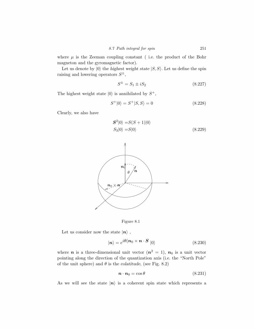
Let us consider now the state |n⟩ ,

|n⟩ = eiθ(n0 × n · S |0⟩ (8.230)

where n is a three-dimensional unit vector (n2 = 1), n0 is a unit vectorpointing along the direction of the quantization axis (i.e. the “North Pole”of the unit sphere) and θ is the colatitude, (see Fig. 8.2)

n · n0 = cos θ (8.231)

As we will see the state |n⟩ is a coherent spin state which represents a


spin polarized along the n axis. The state |n⟩ can be expanded in the basis|S,M⟩,

|n⟩ =S∑

M=−S

D(S)MS(n) |S,M⟩ (8.232)

Here D(S)MS(n) are the representation matrices in the spin-S representation.

It is important to note that there are many rotations that lead to thesame state |n⟩ from the highest weight |0⟩. For example any rotation alongthe direction n results only in a change in the phase of the state |n⟩. Theserotations are equivalent to a multiplication on the right by a rotation aboutthe z axis. However, in Quantum Mechanics this phase has no physicallyobservable consequence. Hence we will regard all of these states as beingphysically equivalent. In other terms, the states for equivalence classes (orrays) and we must pick one and only one state from each class. These rota-tions are generated by S3, the (only) diagonal generator of SU(2). Hence,the physical states are not in one-to-one correspondence with the elementsof SU(2) but instead with the elements of the right coset SU(2)/U(1), withthe U(1) generated by S3. (In the case of a more general group we mustdivide out the maximal torus generated by all the diagonal generators ofthe group.) In mathematical language, if we consider all the rotations atonce , the spin coherent states are said to form a Hermitian line bundle.

A consequence of these observations is that the D matrices do not forma group under matrix multiplication. Instead they satisfy

D(S)(n1)D(S)(n2) = D(S)(n3) e

iΦ(n1,n2,n3)S3 (8.233)

where the phase factor is usually called a cocycle. Here Φ(n1, n2,n3) is the(oriented) area of the spherical triangle with vertices at n1,n2,n3. However,since the sphere is a closed surface, which area do we actually mean? “Inside”or “outsider”? Thus, the phase factor is ambiguous by an amount determinedby 4π, the total area of the sphere,

ei4πM (8.234)

However, since M is either an integer or a half-integer this ambiguity in Φhas no consequence whatsoever,

ei4πM = 1 (8.235)

(we can also regard this result as a requirement that M be quantized).The states |n⟩ are coherent states which satisfy the following properties


n1 n2

n3

Figure 8.2

(see Perelomov’s book Coherent States). The overlap of two coherent states|n1⟩ and |n2⟩ is

⟨n1|n2⟩ = ⟨0|D(S)(n1)†D(S)(n2)|0⟩

= ⟨0|D(S)(n0)eiΦ(n1,n2, n0)S3 |0⟩

=

(1 +n1 · n2

2

)S

eiΦ(n1,n2,n0)S (8.236)

The (diagonal) matrix element of the spin operator is

⟨n|S|n⟩ = S n (8.237)

Finally, the (over-complete) set of coherent states |n⟩ have a resolution ofthe identity of the form

I =

∫dµ(n) |n⟩⟨n| (8.238)

where the integration measure dµ(n) is

dµ(n) =

(2S + 1

4π

)δ(n2 − 1)d3n (8.239)

Let us now use the coherent states |n⟩ to find the path integral for aspin. In imaginary time τ (and with periodic boundary conditions) the pathintegral is simply the partition function

Z = tre−βH (8.240)


where β = 1/T (T is the temperature) and H is the Hamiltonian. As usualthe path integral form of the partition function is found by splitting up theimaginary time interval 0 ≤ τ ≤ β in Nτ steps each of length δτ such thatNτδτ = β. Hence we have

Z = limNτ→∞,δτ→0

tr(e−δτH

)Nτ

(8.241)

and insert the resolution of the identity at every intermediate time step,


⎛

⎝Nτ∏

j=1

∫dµ(nj)

⎞

⎠

⎛

⎝Nτ∏

j=1

⟨n(τj)|e−δτH |n(τj+1)⟩

⎞

⎠

≃ limNτ→∞,δτ→0

⎛

⎝Nτ∏

j=1

∫dµ(nj)

⎞

⎠

⎛

⎝Nτ∏

j=1

[⟨n(τj)|n(τj+1)⟩ − δτ⟨n(τj)|H|n(τj+1)⟩]

⎞

⎠

(8.242)

However, since

⟨n(τj)|H|n(τj+1)⟩⟨n(τj)|n(τj+1)⟩

≃ ⟨n(τj)|H|n(τj)⟩ = µSB · n(τj) (8.243)

and

⟨n(τj)|n(τj+1)⟩ =(1 + n(τj) · n(τj+1)

2

)S

eiΦ(n(τj),n(τj+1),n0)S

(8.244)we can write the partition function in the form


∫Dn e−SE[n] (8.245)

where SE[n] is given by

−SE[n] = iSNτ∑

j=1

Φ(n(τj), n(τj+1),n0)

+SNτ∑

j=1

ln

(1 + n(τj) · n(τj+1)

2

)−

Nτ∑

j=1

(δτ)µS n(τj) ·B (8.246)

The first term of the right hand side of Eq. (8.256) contains the expressionΦ(n(τj), n(τj+1),n0) which has a simple geometric interpretation: it is thesum of the areas of the Nτ contiguous spherical triangles. These triangleshave the pole n0 as a common vertex, and their other pairs of vertices tracea spherical polygon with vertices at n(τj). In the time continuum limit


this spherical polygon becomes the history of the spin, which traces a closedoriented curve Γ = n(τ) (with 0 ≤ τ ≤ β). Let us denote by Ω+ theregion of the sphere whose boundary is Γ and which contains the pole n0.The complement of this region is Ω− and it contains the opposite pole −n0.Hence we find that

limNτ→∞,δτ→0

Φ(n(τj),n(τj+1),n0) = A[Ω+] = 4π −A[Ω−] (8.247)

where A[Ω] is the area of the region Ω. Once again, the ambiguity of thearea leads to the requirement that S should be an integer or a half-integer.

n(τj)

n0

n(τj+1

Ω+

Ω−

Figure 8.3

There is a simple an elegant way to write the area enclosed by Γ. Letn(τ) be a history and Γ be the set of points o the 2-sphere traced by n(τ)for 0 ≤ τ ≤ β. Let us define n(τ, s) (with 0 ≤ s ≤ 1) to be an arbitrary

extension of n(τ) from the curve Γ to the interior of the upper cap Ω+, suchthat

n(τ, 0) = n(τ)

n(τ, 1) = n0

n(τ, 0) = n(τ + β, 0)

(8.248)

Then the area can be written in the compact form

A[Ω+] =

∫ 1

0ds

∫ β

0dτ n(τ, s) · ∂τn(τ, s)× ∂sn(τ, s) ≡ SWZ[n] (8.249)


In Mathematics this expression for the area is called the (simplectic) 2-form,and in the Physics literature is usually called a Wess-Zumino action, SWZ,or Berry Phase.

Φ = 4πSTotal Flux

Figure 8.4 A hairy ball or monopole

Thus, in the (formal) time continuum limit, the action SE becomes

SE = −iS SWZ[n] +Sδτ

2

∫ β

0dτ (∂τn(τ))

2 +

∫ β

0dτ µS B · n(τ) (8.250)

Notice that we have kept (temporarily) a term of order δτ , which we willdrop shortly.

How do we interpret Eq. (8.250)? Since n(τ) is constrained to be a pointon the surface of the unit sphere, i.e. n2 = 1, the action SE[n] can beinterpreted as the action of a particle of mass M = Sδτ → 0 and n(τ) isthe position vector of the particle at (imaginary) time τ . Thus, the secondterm is a (vanishingly small) kinetic energy term, and the last term of Eq.(8.250) is a potential energy term.

What is the meaning of the first term? In Eq. (8.249) we saw that SWZ[n],the the so-called Wess-Zumino or Berry phase term in the action, is the areaof the (positively oriented) region A[Ω+] “enclosed” by the “path” n(τ). Infact,

SWZ[n] =

∫ 1

0ds

∫ β

0dτn · ∂τn× ∂sn (8.251)

is the area of the oriented surface Ω+ whose boundary is the oriented pathΓ = ∂Ω+ (see Fig. 8.3). Using Stokes theorem we can write the the expression


SA[n] as the circulation of a vector field A[n],∮

∂Ωdn ·A[n(τ)] =

∫∫

Ω+dS ·n ×A[n(τ)] (8.252)

provided the “magnetic field” n ×A is “constant”, namely

B = n ×A[(τ)] = S n(τ) (8.253)

What is the total flux Φ of this magnetic field?

Φ =

∫

spheredS ·n ×A[n]

= S

∫dS · n ≡ 4πS (8.254)

Thus, the total number of flux quanta Nφ piercing the unit sphere is

Nφ =Φ

2π= 2S = magnetic charge (8.255)

We reach the condition that the magnetic charge is quantized, a result knownas the Dirac quantization condition.

Is this result consistent with what we know about charged particles inmagnetic fields? In particular, how is this result related to the physics ofspin? To answer these questions we will go back to real time and write theaction

S[n] =∫ T

0dt

[M

2

(dn

dt

)2

+A[n(t)] · dndt− µSn(t) ·B

]

(8.256)

with the constraint n 2 = 1 and where the limit M → 0 is implied.The classical hamiltonian associated to the action of Eq. (8.256) is

H =1

2M[n× (p−A[n])]2 + µSn ·B ≡ H0 + µSn ·B (8.257)

It is easy to check that the vector Λ,

Λ = n× (p−A) (8.258)

satisfies the algebra

[Λa,Λb] = i!ϵabc (Λc − !Snc) (8.259)

where a, b, c = 1, 2, 3, ϵabc is the (third rank) Levi-Civita tensor, and with

Λ · n = n ·Λ = 0 (8.260)


the generators of rotations for this system are

L = Λ+ !Sn (8.261)

The operators L and Λ satisfy the (joint) algebra

[La, Lb] = −i!ϵabcLs[La,L2

]= 0

[La, nb] = i!ϵabcnc [La,Λb] = i!ϵabcΛc

(8.262)

Hence[La,Λ

2]= 0 ⇒ [La,H] = 0 (8.263)

since the operators La satisfy the angular momentum algebra, we can diago-nalize L2 and L3 simultaneously. Let |m, ℓ⟩ be the simultaneous eigenstatesof L2 and L3,

L2|m, ℓ⟩ = !2ℓ(ℓ+ 1)|m, ℓ⟩ (8.264)

L3|m, ℓ⟩ = !m|m, ℓ⟩ (8.265)

H0|m, ℓ⟩ = !2

2MR2

(ℓ(ℓ+ 1)− S

2S

)|m, ℓ⟩ (8.266)

where R = 1 is the radius of the sphere. The eigenvalues ℓ are of the formℓ = S + n, |m| ≤ ℓ, with n ∈ Z+ ∪ 0 and 2S ∈ Z+ ∪ 0. Hence each levelis 2ℓ+1-fold degenerate, or what is equivalent, 2n+1+2S-fold degenerate.Then, we get

Λ 2 = L 2 − n 2!2S2 = L 2 − !

2S2 (8.267)

Since M = Sδt→ 0, the lowest energy in the spectrum of H0 are those withthe smallest value of ℓ, i. e. states with n = 0 and ℓ = S. The degeneracy ofthis “Landau” level is 2S+1, and the gap to the next excited states divergesas M → 0. Thus, in the M → 0 limit, the lowest energy states have the samedegeneracy as the spin-S representation. Moreover, the operators L 2 andL3 become the corresponding spin operators. Thus, the equivalency foundis indeed correct.

Thus, we have shown that the quantum states of a scalar (non-relativistic)particle bound to a magnetic monopole of magnetic charge 2S, obeying theDirac quantization condition, are identical to those of those of a spinningparticle!

We close this section with some observations on the semi-classical motion.From the (real time) action (already in the M → 0 limit)

S = −∫ T

0dt µS n ·B + S

∫ T

0dt

∫ 1

0ds n · ∂tn× ∂sn (8.268)


we can derive a Classical Equation of Motion by looking at the stationaryconfigurations. The variation of the second term in Eq. (8.268) is

δS = S δ

∫ T

0dt

∫ 1

0ds n · ∂tn× ∂sn = S

∫ T

0dtδn(t) ·n(t)× ∂tn(t) (8.269)

the variation of the first term in Eq. (8.268) is

δ

∫ T

0dt µSn(t) ·B =

∫ T

0dt δn(t) · µSB (8.270)

Hence,

δS =

∫ T

0dt δn(t) · (−µSB + Sn(t)× ∂tn(t)) (8.271)

which implies that the classical trajectories must satisfy the equation ofmotion

µB = n× ∂tn (8.272)

If we now use the vector identity

n× n× ∂tn = (n · ∂tn)n−n 2∂tn (8.273)

and

n · ∂tn = 0, and n 2 = 1 (8.274)

we get the classical equation of motion

∂tn = µB ×n (8.275)

Therefore, the classical motion is precessional with an angular velocity Ωpr =µB.

9

Quantization of Gauge Fields

We will now turn to the problem of the quantization of gauge theories. Wewill begin with the simplest gauge theory, the free electromagnetic field.This is an abelian gauge theory. After that we will discuss at length thequantization of non-abelian gauge fields. Unlike abelian theories, such as thefree electromagnetic field, even in the absence of matter fields non-abeliangauge theories are not free fields and have highly non-trivial dynamics.

9.1 Canonical Quantization of the Free Electromagnetic Field

Maxwell’s theory was the first field theory to be quantized. However, thequantization procedure involves a number of subtleties not shared by theother problems that we have considered so far. The issue is the fact that thistheory has a local gauge invariance. Unlike systems which only have globalsymmetries, not all the classical configurations of vector potentials representphysically distinct states. It could be argued that one should abandon thepicture based on the vector potential and go back to a picture based onelectric and magnetic fields instead. However, there is no local Lagrangianthat can describe the time evolution of the system now. Furthermore is notclear which fields, E or B (or some other field) plays the role of coordinatesand which can play the role of momenta. For that reason, one sticks tothe Lagrangian formulation with the vector potential Aµ as its independentcoordinate-like variable.

The Lagrangian for Maxwell’s theory

L = −1

4FµνF

µν (9.1)

Coherent State Path Integral Quantization of Quantum Field...

Documents

Transcript of Coherent State Path Integral Quantization of Quantum Field...