Coherent Spin Dynamics of a Spin-1 Bose-Einstein

Condensate

A ThesisPresented to

The Academic Faculty

by

Ming-Shien Chang

In Partial Fulfillmentof the Requirements for the Degree

Doctor of Philosophy

School of PhysicsGeorgia Institute of Technology

May 2006

Coherent Spin Dynamics of a Spin-1 Bose-Einstein

Condensate

Approved by:

Professor Michael S. ChapmanSchool of Physics, Chair

Professor T. A. Brian KennedySchool of Physics

Professor Chandra RamanSchool of Physics

Professor Alex KuzmichSchool of Physics

Professor Gee-Kung ChangSchool of Electrical and Computer Engi-neering

Date Approved: March, 29, 2006

To my parents,

Mr. Muh-Yen Chang and Mrs. Hsueh-Huang Chang

iii

ACKNOWLEDGEMENTS

I would like to take this opportunity to thank the people who have inspired and supported

me throughout my PhD studies. First, I would like to express my greatest gratitude to my

advisor, Prof. Michael Chapman. Mike has amazing physics intuition and talent for solving

challenging technical problems simply and cleverly. His great insight and capability has

helped us from going in wrong directions to search for answers. Mike taught me how to

be a good experimentalist. However, perhaps the more valuable things I learned from him

are his optimistic attitude and leadership. I will offer two examples to demonstrate Mike’s

leadership. One day, I realized that our experiment control center, a heavy table hosting

computers and power equipment, was too close to our vacuum chamber, and the magnetic

noise from this table was badly affecting our measurements. Mike knew that I was going

to move the control center in an evening. So he showed up that night, and we ended up

moving heavy instruments and tossing perhaps 50 cables across the lab at midnight. While

working on creating BECs in a single focus trap, we decided to compress the trap. Again,

Mike was the person who pushed a manual translation stage for me in the late night for

few hours, and, that night, we made the first “hand-made” BECs in the single focus trap.

For Mike’s advice and great leadership, he has my highest regard.

Next, I would like to extend my gratitude to Prof. Brian Kennedy, Li You, Chandra

Raman, and Alex Kuzmich, for offering their expertise and physics insight through many

stimulating discussions. Especially Brian, he always patiently cleared up my thoughts

through rigorous deductions no matter how minute the questions I had.

I am grateful to work with several wonderful and talented lab colleagues after I arrived

Georgia Tech. Prof. Murray Barrett was finishing up his thesis when I joined the lab.

Working with Murray was very productive, and his determination and diligence really im-

pressed me and has continued to inspire me throughout these years. After Murray left, Dr.

Jacob Sauer helped me to quickly fill my knowledge gap on running the experiment with

iv

his great experience. Jake is a versatile physicist with a vivid personality; it is always fun

to have Jake involved, either at work of after school. Kevin Fortier not only works hard and

sets a high standard on work ethics, but is a very good friend after school. Chris Hamley

is a special and talented undergraduate student. His electronics knowledge and hands-on

skills are far beyond what an undergraduate student should know. His beautiful work on

the microwave electronics and horn have made our spinor studies possible. The beautiful

Thor’s Hammer (glass cell) he built is still awaiting to be turned into a BEC chamber.

I am also grateful to work with my theory collaborator, Dr. Wenxian Zhang. I have

learned much physics of spinor condensates through countless discussions with him. I am

also indebted to Wenxian for the numerical simulations he has done, which provided valuable

insights for our spinor experiments.

I wish to thank our new postdoc Dr. Paul Griffin, and my junior colleagues, Qishu

Qin, Eva Bookjans, Sally Maddocks, Shane Allman, Soo Kim, Michael Gibbons, Adam

Steele, and Layne Churchill for their great help on the experiments, thesis proofread, and

for companionship. I also would like to acknowledge colleagues from other groups. I have

enjoyed discussing physics with Devang Naik, Stewart Jenkins, Dzmitry Matsukevich, Dr.

Mishkatul Bhattacharya, Dr. Sergio Muniz, and others in the Journal Club.

Special thanks to Prof. Glenn Edwards of Duke Physics and Free Electron Laser Lab-

oratory, and my good friend, Dr. Meng-Ru Li. Glenn was a kind advisor when I worked

with him on biophysics, and his wise encouragement has continued to inspire me throughout

these years. I would never thought of joining Georgia Tech were it not for an accidental

crossover between Meng-Ru and Prof. Li You in a biophysics summer school. Meng-Ru

mentioned my existence to Li, which in turn led to my great adventure at Tech.

Finally, I would like to thank my parents and my sisters for their unconditional and

endless love and support throughout my endeavor. Their constant support make what I am

today. For that, I am forever indebted to them.

Georgia Institute of Technology

May 2006

v

TABLE OF CONTENTS

DEDICATION . . . . . . . . . . . . . . . . . . . . . . . . . . . . . . . . . . . . . . iii

ACKNOWLEDGEMENTS . . . . . . . . . . . . . . . . . . . . . . . . . . . . . . iv

LIST OF TABLES . . . . . . . . . . . . . . . . . . . . . . . . . . . . . . . . . . . ix

LIST OF FIGURES . . . . . . . . . . . . . . . . . . . . . . . . . . . . . . . . . . x

SUMMARY . . . . . . . . . . . . . . . . . . . . . . . . . . . . . . . . . . . . . . . . xiii

I INTRODUCTION . . . . . . . . . . . . . . . . . . . . . . . . . . . . . . . . . 1

1.1 A Brief Review of Bose-Einstein Condensation . . . . . . . . . . . . . . . . 1

1.2 Spinor Condensates . . . . . . . . . . . . . . . . . . . . . . . . . . . . . . . 3

1.3 Thesis Overview . . . . . . . . . . . . . . . . . . . . . . . . . . . . . . . . . 5

II THE EXPERIMENTAL SETUP . . . . . . . . . . . . . . . . . . . . . . . . 6

2.1 Rubidium-87 Properties . . . . . . . . . . . . . . . . . . . . . . . . . . . . 6

2.2 Magneto-Optical Trap . . . . . . . . . . . . . . . . . . . . . . . . . . . . . 9

2.2.1 Diode Lasers . . . . . . . . . . . . . . . . . . . . . . . . . . . . . . . 11

2.2.2 Laser Frequency Stabilization and Tuning . . . . . . . . . . . . . . 12

2.2.3 Magnetic Coils . . . . . . . . . . . . . . . . . . . . . . . . . . . . . 13

2.3 Vacuum Chamber and Atom Source . . . . . . . . . . . . . . . . . . . . . . 17

2.4 Optical Dipole Force Trap . . . . . . . . . . . . . . . . . . . . . . . . . . . 18

2.4.1 Optical Trap Parameters . . . . . . . . . . . . . . . . . . . . . . . . 22

2.5 Atom Probe and Signal Collection . . . . . . . . . . . . . . . . . . . . . . . 24

2.6 Microwave Source . . . . . . . . . . . . . . . . . . . . . . . . . . . . . . . . 25

2.7 Control Unit . . . . . . . . . . . . . . . . . . . . . . . . . . . . . . . . . . . 25

III DETECTION AND IMAGE ANALYSIS FOR ULTRACOLD ATOMICCLOUDS . . . . . . . . . . . . . . . . . . . . . . . . . . . . . . . . . . . . . . . 27

3.1 Measurement Techniques for Ultracold Atoms . . . . . . . . . . . . . . . . 28

3.1.1 Fluorescence Imaging . . . . . . . . . . . . . . . . . . . . . . . . . . 28

3.1.2 Absorption Imaging . . . . . . . . . . . . . . . . . . . . . . . . . . . 29

3.2 Measurements for Ultracold Gases . . . . . . . . . . . . . . . . . . . . . . . 31

3.3 Image Analysis for Ultracold Clouds Near BEC Transition Temperatures . 37

vi

IV ALL-OPTICAL BEC EXPERIMENTS . . . . . . . . . . . . . . . . . . . . 47

4.1 Review of First All-Optical BEC . . . . . . . . . . . . . . . . . . . . . . . 47

4.2 Trap Loading Studies . . . . . . . . . . . . . . . . . . . . . . . . . . . . . . 49

4.3 Bose Condensation in 1D Lattice . . . . . . . . . . . . . . . . . . . . . . . 53

4.3.1 Measurement and Control of The Lattice Sites Occupied . . . . . . 54

4.3.2 Matter Wave Interference . . . . . . . . . . . . . . . . . . . . . . . 56

4.4 Bose Condensation in a Single Focus Trap . . . . . . . . . . . . . . . . . . 58

V SPINOR CONDENSATE THEORY . . . . . . . . . . . . . . . . . . . . . 68

5.1 Microscopic picture . . . . . . . . . . . . . . . . . . . . . . . . . . . . . . . 69

5.2 Second Quantized Hamiltonian for Spin-1 Condensates . . . . . . . . . . . 72

5.3 Spinors In Magnetic Fields . . . . . . . . . . . . . . . . . . . . . . . . . . . 74

5.4 Coupled Gross-Pitaevskii equations for spin-1 condensates . . . . . . . . . 76

5.5 Single-Mode approximation . . . . . . . . . . . . . . . . . . . . . . . . . . 78

VI OBSERVATION OF SPINOR DYNAMICS IN F=1 AND F=2 BOSECONDENSATES . . . . . . . . . . . . . . . . . . . . . . . . . . . . . . . . . . 81

6.1 Formation of Spinor Condensates . . . . . . . . . . . . . . . . . . . . . . . 81

6.2 Spinor Ground State . . . . . . . . . . . . . . . . . . . . . . . . . . . . . . 86

6.3 Observation of Spin-2 Dynamics . . . . . . . . . . . . . . . . . . . . . . . . 93

VII COHERENT SPINOR DYNAMICS . . . . . . . . . . . . . . . . . . . . . 96

7.1 Initiation of Coherent Spin Mixing . . . . . . . . . . . . . . . . . . . . . . 97

7.2 Measuring c2 . . . . . . . . . . . . . . . . . . . . . . . . . . . . . . . . . . . 99

7.3 Controlling Coherent Spin Mixing . . . . . . . . . . . . . . . . . . . . . . . 100

7.4 Coherence of the Ferromagnetic Ground State . . . . . . . . . . . . . . . . 101

VIII SPIN DOMAIN FORMATION IN FERROMAGNETIC SPIN-1 CON-DENSATES . . . . . . . . . . . . . . . . . . . . . . . . . . . . . . . . . . . . . 107

8.1 Miscibility of Spin Components . . . . . . . . . . . . . . . . . . . . . . . . 110

8.2 Spin Wave and Domain Formation in Ferromagnetic Condensates . . . . . 112

8.3 Study of The Validity of Single-Mode Approximation . . . . . . . . . . . . 116

IX FINAL REMARKS . . . . . . . . . . . . . . . . . . . . . . . . . . . . . . . . 121

APPENDIX A — TABLE OF CONSTANTS AND PROPERTIES OF87RB . . . . . . . . . . . . . . . . . . . . . . . . . . . . . . . . . . . . . . . . . . 123

vii

APPENDIX B — SPINOR DEGREES OF FREEDOM OF TWO SPIN-FATOMS UNDER COLLISION . . . . . . . . . . . . . . . . . . . . . . . . . 124

APPENDIX C — SPIN COUPLING OF TWO SPIN-1 ATOMS . . . . 126

APPENDIX D — INTERACTION HAMILTONIAN OF SPIN-1 BOSEGAS . . . . . . . . . . . . . . . . . . . . . . . . . . . . . . . . . . . . . . . . . . 128

APPENDIX E — SPINOR ENERGY FUNCTIONAL AND MEAN-FIELDGROUND STATES . . . . . . . . . . . . . . . . . . . . . . . . . . . . . . . . 130

APPENDIX F — PROCEDURE FOR EXTRACTING C 2 . . . . . . . . 133

REFERENCES . . . . . . . . . . . . . . . . . . . . . . . . . . . . . . . . . . . . . 136

viii

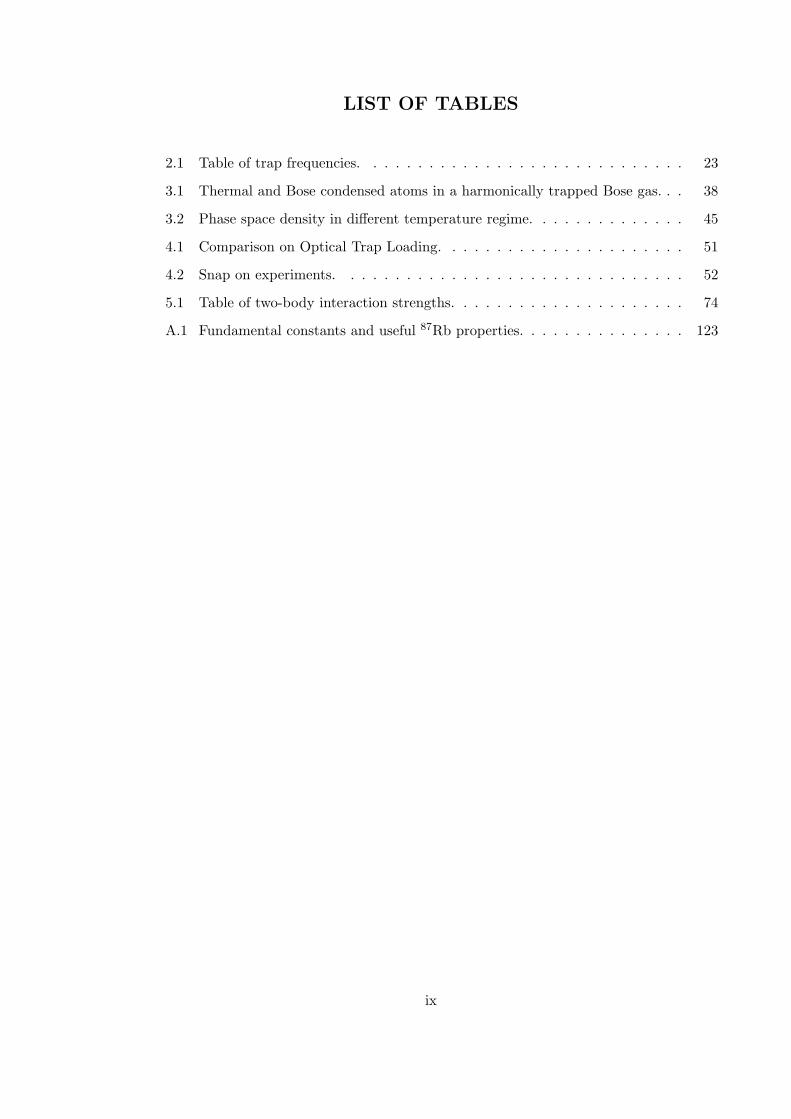
LIST OF TABLES

2.1 Table of trap frequencies. . . . . . . . . . . . . . . . . . . . . . . . . . . . . 23

3.1 Thermal and Bose condensed atoms in a harmonically trapped Bose gas. . . 38

3.2 Phase space density in different temperature regime. . . . . . . . . . . . . . 45

4.1 Comparison on Optical Trap Loading. . . . . . . . . . . . . . . . . . . . . . 51

4.2 Snap on experiments. . . . . . . . . . . . . . . . . . . . . . . . . . . . . . . 52

5.1 Table of two-body interaction strengths. . . . . . . . . . . . . . . . . . . . . 74

A.1 Fundamental constants and useful 87Rb properties. . . . . . . . . . . . . . . 123

ix

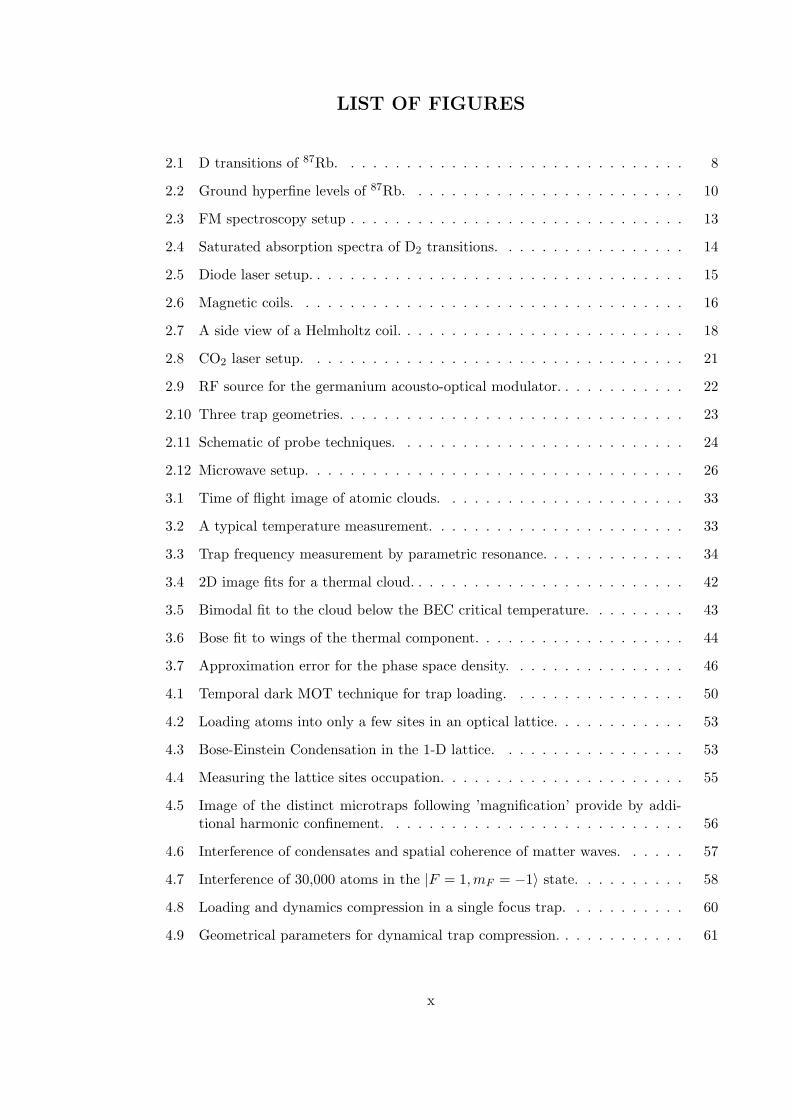
LIST OF FIGURES

2.1 D transitions of 87Rb. . . . . . . . . . . . . . . . . . . . . . . . . . . . . . . 8

2.2 Ground hyperfine levels of 87Rb. . . . . . . . . . . . . . . . . . . . . . . . . 10

2.3 FM spectroscopy setup . . . . . . . . . . . . . . . . . . . . . . . . . . . . . . 13

2.4 Saturated absorption spectra of D2 transitions. . . . . . . . . . . . . . . . . 14

2.5 Diode laser setup. . . . . . . . . . . . . . . . . . . . . . . . . . . . . . . . . . 15

2.6 Magnetic coils. . . . . . . . . . . . . . . . . . . . . . . . . . . . . . . . . . . 16

2.7 A side view of a Helmholtz coil. . . . . . . . . . . . . . . . . . . . . . . . . . 18

2.8 CO2 laser setup. . . . . . . . . . . . . . . . . . . . . . . . . . . . . . . . . . 21

2.9 RF source for the germanium acousto-optical modulator. . . . . . . . . . . . 22

2.10 Three trap geometries. . . . . . . . . . . . . . . . . . . . . . . . . . . . . . . 23

2.11 Schematic of probe techniques. . . . . . . . . . . . . . . . . . . . . . . . . . 24

2.12 Microwave setup. . . . . . . . . . . . . . . . . . . . . . . . . . . . . . . . . . 26

3.1 Time of flight image of atomic clouds. . . . . . . . . . . . . . . . . . . . . . 33

3.2 A typical temperature measurement. . . . . . . . . . . . . . . . . . . . . . . 33

3.3 Trap frequency measurement by parametric resonance. . . . . . . . . . . . . 34

3.4 2D image fits for a thermal cloud. . . . . . . . . . . . . . . . . . . . . . . . . 42

3.5 Bimodal fit to the cloud below the BEC critical temperature. . . . . . . . . 43

3.6 Bose fit to wings of the thermal component. . . . . . . . . . . . . . . . . . . 44

3.7 Approximation error for the phase space density. . . . . . . . . . . . . . . . 46

4.1 Temporal dark MOT technique for trap loading. . . . . . . . . . . . . . . . 50

4.2 Loading atoms into only a few sites in an optical lattice. . . . . . . . . . . . 53

4.3 Bose-Einstein Condensation in the 1-D lattice. . . . . . . . . . . . . . . . . 53

4.4 Measuring the lattice sites occupation. . . . . . . . . . . . . . . . . . . . . . 55

4.5 Image of the distinct microtraps following ’magnification’ provide by addi-tional harmonic confinement. . . . . . . . . . . . . . . . . . . . . . . . . . . 56

4.6 Interference of condensates and spatial coherence of matter waves. . . . . . 57

4.7 Interference of 30,000 atoms in the |F = 1,mF = −1〉 state. . . . . . . . . . 58

4.8 Loading and dynamics compression in a single focus trap. . . . . . . . . . . 60

4.9 Geometrical parameters for dynamical trap compression. . . . . . . . . . . . 61

x

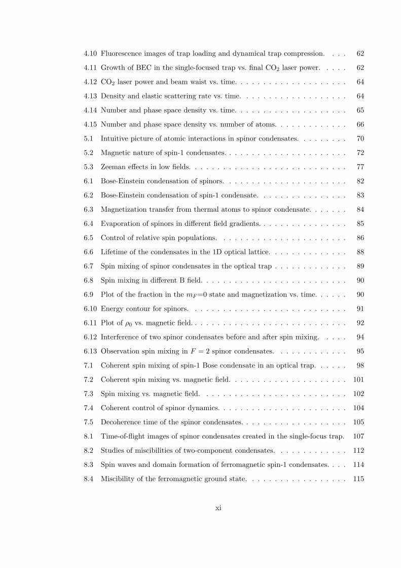
4.10 Fluorescence images of trap loading and dynamical trap compression. . . . 62

4.11 Growth of BEC in the single-focused trap vs. final CO2 laser power. . . . . 62

4.12 CO2 laser power and beam waist vs. time. . . . . . . . . . . . . . . . . . . . 64

4.13 Density and elastic scattering rate vs. time. . . . . . . . . . . . . . . . . . . 64

4.14 Number and phase space density vs. time. . . . . . . . . . . . . . . . . . . . 65

4.15 Number and phase space density vs. number of atoms. . . . . . . . . . . . . 66

5.1 Intuitive picture of atomic interactions in spinor condensates. . . . . . . . . 70

5.2 Magnetic nature of spin-1 condensates. . . . . . . . . . . . . . . . . . . . . . 72

5.3 Zeeman effects in low fields. . . . . . . . . . . . . . . . . . . . . . . . . . . . 77

6.1 Bose-Einstein condensation of spinors. . . . . . . . . . . . . . . . . . . . . . 82

6.2 Bose-Einstein condensation of spin-1 condensate. . . . . . . . . . . . . . . . 83

6.3 Magnetization transfer from thermal atoms to spinor condensate. . . . . . . 84

6.4 Evaporation of spinors in different field gradients. . . . . . . . . . . . . . . . 85

6.5 Control of relative spin populations. . . . . . . . . . . . . . . . . . . . . . . 86

6.6 Lifetime of the condensates in the 1D optical lattice. . . . . . . . . . . . . . 88

6.7 Spin mixing of spinor condensates in the optical trap . . . . . . . . . . . . . 89

6.8 Spin mixing in different B field. . . . . . . . . . . . . . . . . . . . . . . . . . 90

6.9 Plot of the fraction in the mF =0 state and magnetization vs. time. . . . . . 90

6.10 Energy contour for spinors. . . . . . . . . . . . . . . . . . . . . . . . . . . . 91

6.11 Plot of ρ0 vs. magnetic field. . . . . . . . . . . . . . . . . . . . . . . . . . . . 92

6.12 Interference of two spinor condensates before and after spin mixing. . . . . 94

6.13 Observation spin mixing in F = 2 spinor condensates. . . . . . . . . . . . . 95

7.1 Coherent spin mixing of spin-1 Bose condensate in an optical trap. . . . . . 98

7.2 Coherent spin mixing vs. magnetic field. . . . . . . . . . . . . . . . . . . . . 101

7.3 Spin mixing vs. magnetic field. . . . . . . . . . . . . . . . . . . . . . . . . . 102

7.4 Coherent control of spinor dynamics. . . . . . . . . . . . . . . . . . . . . . . 104

7.5 Decoherence time of the spinor condensates. . . . . . . . . . . . . . . . . . . 105

8.1 Time-of-flight images of spinor condensates created in the single-focus trap. 107

8.2 Studies of miscibilities of two-component condensates. . . . . . . . . . . . . 112

8.3 Spin waves and domain formation of ferromagnetic spin-1 condensates. . . . 114

8.4 Miscibility of the ferromagnetic ground state. . . . . . . . . . . . . . . . . . 115

xi

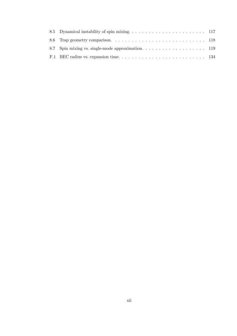
8.5 Dynamical instability of spin mixing. . . . . . . . . . . . . . . . . . . . . . . 117

8.6 Trap geometry comparison. . . . . . . . . . . . . . . . . . . . . . . . . . . . 118

8.7 Spin mixing vs. single-mode approximation. . . . . . . . . . . . . . . . . . . 119

F.1 BEC radius vs. expansion time. . . . . . . . . . . . . . . . . . . . . . . . . . 134

xii

SUMMARY

Bose-Einstein condensation (BEC) is a well-known phenomenon in which identical

bosons occupy the same quantum state below a certain critical temperature. A hallmark

of BEC is the coherence between particles — every particle shares the same quantum wave

function and phase. This matter wave coherence has been demonstrated for the external

(motional) degrees of freedom by interfering two condensates. In this thesis, we show

that the coherence extends to the internal spin degrees of freedom of a spin-1 Bose gas by

observing coherent and reversible spin-changing collisions. The observed coherent dynamics

are analogous to Josephson oscillations in weakly connected superconductors and represent

a type of matter-wave four-wave mixing. We also demonstrate control of the coherent

evolution of the system using magnetic fields.

In the first part of this thesis, the all-optical approaches to BEC that were first developed

in our laboratory will be introduced. All-optical formation of Bose-Einstein condensates

(BEC) in 1D optical lattice and single focus trap geometries will be presented. These

techniques offer considerable flexibility and speed compared to magnetic trap approaches,

and the trapping potential can be essentially spin-independent. These optical traps are

ideally suited for studying condensates with internal spin degrees of freedom, so-called

spinor condensates.

The second part of this thesis will be devoted to the study of spinor condensates. This

new form of coherent matter exhibits complex internal structure, and the delicate inter-

play of the different magnetic quantum gases yields a rich variety of phenomenon including

coherent spin mixing and spin domain formation. We begin our study on spinor conden-

sates by tailoring the internal spin states of the spinor condensate. Using condensates with

well-defined initially non-equilibrium spin configuration, spin mixing of F = 1 and F = 2

spinor condensates of 87Rb atoms confined in an optical trap is observed. The equilibrium

spin configuration in the F = 1 manifold is measured from which we confirm 87Rb to be

xiii

ferromagnetic. The coherent spinor dynamics are demonstrated by initiating spin mixing

deterministically with a non-stationary spin population configuration. Finally, the inter-

play between the coherent spin mixing and spatial dynamics in spin-1 condensates with

ferromagnetic interactions are investigated.

xiv

CHAPTER I

INTRODUCTION

Bose-Einstein condensation (BEC) in dilute atomic gases was first observed in 1995 [1, 2, 3],

culminating a 20 year effort that began in the 1970s with atomic hydrogen [4, 5] and later

with laser-cooled alkali atoms [6, 7]. Since initial observations of BEC in dilute gases,

research in this field has grown with tremendous momentum, both experimentally and

theoretically. Here we provide a brief and necessarily incomplete review of some of the

developments over the past 11 years to highlight some of the distinctive properties of this

new form of matter and to illustrate the vibrancy of this young research field.

1.1 A Brief Review of Bose-Einstein Condensation

Bose-Einstein condensation is a phenomenon whereby identical bosonic particles lose their

individuality and act in unison as a single quantum entity through macroscopic occupation

of a single quantum state. Condensation into a single quantum state occurs for identical

bosons when the inter-particle separation is less than the thermal de Broglie wavelength

of the particles, or, more precisely, when nλ3dB > 2.612, where n is the particle density

and λdB = h/√

2πmkBT is the thermal de Broglie wavelength. Here, h, kB, m, and T

are the Planck constant, Boltzmann constant, atomic mass, and temperature of the gas,

respectively. For a room temperature gas, λdB is much less than the size of an atom, and

although λdB increases for lower temperature, conventional condensation to liquid or solid

will occur long before reaching the quantum degenerate regime [8]. Hence, an atomic BEC is

a supercooled metastable state that exists in an ultrahigh vacuum chamber, and depending

on the vacuum condition, the lifetime of a condensate ranges from only few seconds to few

minutes [8, 9]. To prevent formation of normal condensed states, which occurs via three-

body collisions leading to molecule formation, atoms must be kept at low densities, typically

on the order of 1014 cm−3, which is 5 orders of magnitude lower than ambient air pressure.

1

At such low densities, atoms need to be cooled to the sub-microKelvin regime in order to

observe Bose-Einstein condensation.

In a Bose condensate, every atom possesses an identical spatial wavefunction, and the

coherent superposition of these wavefunctions results in a macroscopic coherent matter

wave. With a typical atomic diameter of 0.5 A, it is quite extraordinary that the BEC

wavefunction can be as large as 100 µm [10]. This matter wave coherence is perhaps

the most appreciated hallmark of Bose-Einstein condensates, and several experiments have

been devoted to demonstrating and studying this property. The macroscopic matter wave

coherence was first demonstrated by the MIT group by interfering two independent BEC’s

[10]. Later, a type of double-slit experiment performed above and below the BEC transition

temperature by the Munich group demonstrated that there is a fundamental difference

between Bose condensed atoms and thermal atoms [11] — a BEC possesses a macroscopic

wavefunction with a unique phase, while a cloud of thermal atoms does not. The observation

of Josephson tunnelling of BECs between adjacent trapping potential wells demonstrated

tunnelling of these macroscopic wavepackets, which is due to the phase difference between

adjacent BECs [12, 13]. Condensates loaded in a 3D optical lattice have been observed

to show transitions between the Mott-Insulator phase and the superfluidity phase [14],

which showed that phase coherence can be established among many trapping potentials, or

lattice sites, when wavepackets are allowed to tunnel between lattice sites. In analogy with

coherent optical fields, a Bose condensate coupled out of the trap forms a so-called atom

laser [15, 12, 16, 17]. In addition, higher order coherence, such as density correlations of

condensates reflecting the statistical properties of boson fields has also been demonstrated

[18, 19].

Bose-Einstein condensate is a second order phase transition in which bosons begin to

macroscopically occupy the ground state when the temperatures falls below the phase tran-

sition temperature. A hallmark of atomic Bose-Einstein condensates is the relatively weak

and well-characterized inter-atomic interactions that allow quantitative comparison with

theory. Although textbook discussions of Bose-Einstein condensation typically focus on

non-interacting (ideal) particles, interactions between the atoms, via elastic inter-atomic

2

collisions, are required for a trapped gas to reach thermal equilibrium and for evaporative

cooling of the gas to quantum degeneracy. Atomic interactions also affect the ground state

and the dynamical properties of a BEC [20, 21]. In particular, repulsive interactions are

required to maintain a large condensate from collapsing [22, 23].

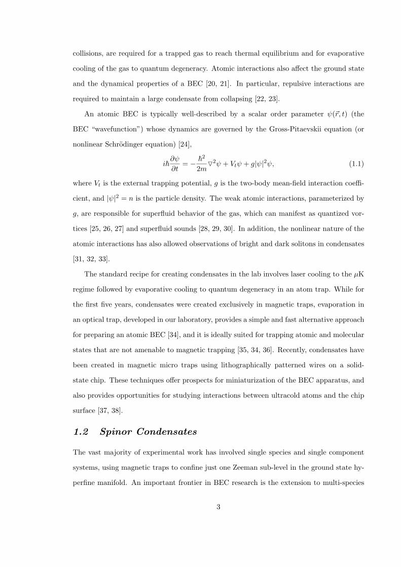
An atomic BEC is typically well-described by a scalar order parameter ψ(~r, t) (the

BEC “wavefunction”) whose dynamics are governed by the Gross-Pitaevskii equation (or

nonlinear Schrodinger equation) [24],

i~∂ψ

∂t= − ~

2

2mO2ψ + Vtψ + g|ψ|2ψ, (1.1)

where Vt is the external trapping potential, g is the two-body mean-field interaction coeffi-

cient, and |ψ|2 = n is the particle density. The weak atomic interactions, parameterized by

g, are responsible for superfluid behavior of the gas, which can manifest as quantized vor-

tices [25, 26, 27] and superfluid sounds [28, 29, 30]. In addition, the nonlinear nature of the

atomic interactions has also allowed observations of bright and dark solitons in condensates

[31, 32, 33].

The standard recipe for creating condensates in the lab involves laser cooling to the µK

regime followed by evaporative cooling to quantum degeneracy in an atom trap. While for

the first five years, condensates were created exclusively in magnetic traps, evaporation in

an optical trap, developed in our laboratory, provides a simple and fast alternative approach

for preparing an atomic BEC [34], and it is ideally suited for trapping atomic and molecular

states that are not amenable to magnetic trapping [35, 34, 36]. Recently, condensates have

been created in magnetic micro traps using lithographically patterned wires on a solid-

state chip. These techniques offer prospects for miniaturization of the BEC apparatus, and

also provides opportunities for studying interactions between ultracold atoms and the chip

surface [37, 38].

1.2 Spinor Condensates

The vast majority of experimental work has involved single species and single component

systems, using magnetic traps to confine just one Zeeman sub-level in the ground state hy-

perfine manifold. An important frontier in BEC research is the extension to multi-species

3

and multi-component systems, which provides a unique opportunity to explore coupled, in-

teracting quantum fluids. In particular, atomic BECs with internal spin degrees of freedom,

or the so-called spinor condensates, offer a new form of coherent matter with complex inter-

nal quantum structures. These multi-component BEC systems are related to other macro-

scopic quantum systems in which internal degrees of freedom [39, 40, 41, 42, 34, 43, 44, 45]

play a prominent role including superfluid 3He [46, 47], neutron stars [48], p-wave [49] and

d-wave BCS superconductors [50], while offering the exquisite control and microscopic un-

derstanding characteristic of weakly interacting quantum degenerate gases. In this thesis,

we focus our studies on the dynamics of spinor condensates in optical traps.

The first two-component condensate was produced utilizing two hyperfine states of 87Rb,

and remarkable phenomena such as phase separation and Rabi oscillations between these

two components were observed [41, 51]. Sodium F = 1 spinor BECs have been created

by transferring spin polarized condensates into a far-off resonant optical trap to liberate

the internal spin degrees of freedom [35]. This allowed investigations of the ground state

properties of Na spinor condensates, and observations of domain structures, metastability,

and quantum spin tunneling [42, 52, 53].

A single-component BEC is described by a scalar order parameter, and its dynamics

are governed by Eq. 1.1. For spinor condensates, the formalism is extended to a vector

order parameter ~ψ = [ψF , ψF−1, · · · , ψ−F ]T, which possesses 2F + 1 components for spin-F

condensates [39, 40] and is invariant under rotation in spin space [39, 40, 54]. For F = 1,

the two-body interaction energy including spin is U(r) = δ(r)(c0 + c2~F1 · ~F2), where r is the

distance between two atoms and c2 is the spin dependent mean-field interaction coefficient.

For F = 2, U(r) = δ(r)(α + β ~F1 · ~F2 + 5γP0), where α is a spin-independent coefficient, β

and γ are spin-dependent coefficients, and P0 is the projection operator [39, 40].

For a spin-1 BEC, the condensate is either ferromagnetic or anti-ferromagnetic [39], and

the corresponding ground state structure and dynamical properties of these two cases are

very distinct. The Na F = 1 spinor was found to be anti-ferromagnetic, while the F = 1

87Rb was predicted to be ferromagnetic [55, 56]. Even richer dynamics are predicted for

spin-2 condensates [50], although they remain largely unexplored experimentally [43, 44].

4

1.3 Thesis Overview

In the first part of this thesis, we will describe our all-optical BEC experiments and present

the creation of condensates in two new trap geometries. In the second part of the thesis, we

will present the results of the studies on the dynamics of spinor condensates in our optical

traps.

Chapter 2 describes our BEC experiment setup. The basic atomic physics and properties

of 87Rb relevant to this thesis are given. The background and implementation of laser

cooling and optical dipole force trap are also briefly summarized. Chapter 3 introduces the

probe techniques we use in our experiment to measure the properties of the ultracold gas.

In Chapter 4 the loading dynamics of different trap geometries are examined. The

understanding gained from these studies has allowed us to create BECs in several different

trap arrangements including a cross trap geometry [34], a 1D optical lattice geometry, and

a single focus geometry. This latter configuration has resulted in a 10-fold increase in the

number of condensed atoms in our experiments.

Chapters 5 to 8 are devoted to the studies of spinor condensates in optical traps. Chap-

ter 5 introduces the microscopic theory of spinor condensates and spinor dynamics to provide

the theoretical foundation of our experimental results. Chapter 6 details the experimen-

tal observation of the individual spinor components and spinor dynamics. In Chapter 7

coherent spinor dynamics, notably spin mixing, are examined. The ability to coherently

control the spin mixing and the spinor ground state is demonstrated. The spatial dynamics

of spinor condensates are examined in further details in Chapter 8. Observations of spin

waves and spin domain formation are presented.

Chapter 9 concludes this thesis, and provides some final remarks and possible future

research directions.

5

CHAPTER II

THE EXPERIMENTAL SETUP

Bose-Einstein Condensation (BEC) in a dilute atomic gas was first achieved in 1995 [1, 2, 3]

by evaporative cooling a laser cooled atomic gas in a magnetic trap. Since then, this basic

technique has been duplicated by over 30 groups worldwide. In this approach, 108 − 1010

atoms are captured and cooled to 100 µK regime in a magneto-optical trap (MOT). In the

MOT, the density is limited to < 1012 cm−3, and the phase space density is 10−6. The

laser cooled atoms are then loaded into a magnetic trap and evaporative cooled to quantum

degeneracy.

An all-optical approach to making condensates was first pioneered in our laboratory in

2001 and provided an alternative, simple and fast approach for preparing atomic conden-

sates. Optical traps can provide tighter confinement for the atoms than a magnetic trap,

and this can lead to higher density and efficient, fast evaporation in the trap. Our BEC

machine consists of a simple vapor cell magneto-optical trap (MOT) and tightly focused

CO2 lasers [34]. This chapter briefly describes our BEC experimental setup.

2.1 Rubidium-87 Properties

The atomic number of rubidium is 37, and the ground state electron configuration is [Kr]5s1,

or 52S1/2 after L-S coupling. The atomic spin is given by ~F = ~I + ~J , where ~I is the nuclear

spin and ~J is the total angular momentum of the valence electron. For rubidium and all

other alkali atoms in the electronic ground state, ~J = ~S and J = S = 1/2 because ~J = ~L+ ~S

and ~L = 0. Here ~L and ~S are the electronic orbital angular momentum and spin. This

results in doublet ground states in all alkali atoms, i.e., Fupper = I+1/2 and Flower = I−1/2.

The nuclear spin of 87Rb is I = 3/2, so Fupper = 2 and Flower = 1. The energy difference

between these two states, the ground hyperfine splitting, is ∼ 6.835 GHz.

The single valence electron of alkalis also leads to two first excited states, which for Rb

6

are the 52P1/2 and 52P3/2 states that are separated by the fine structure splitting. The

optical transitions between the ground state and these excited states constitute the famous

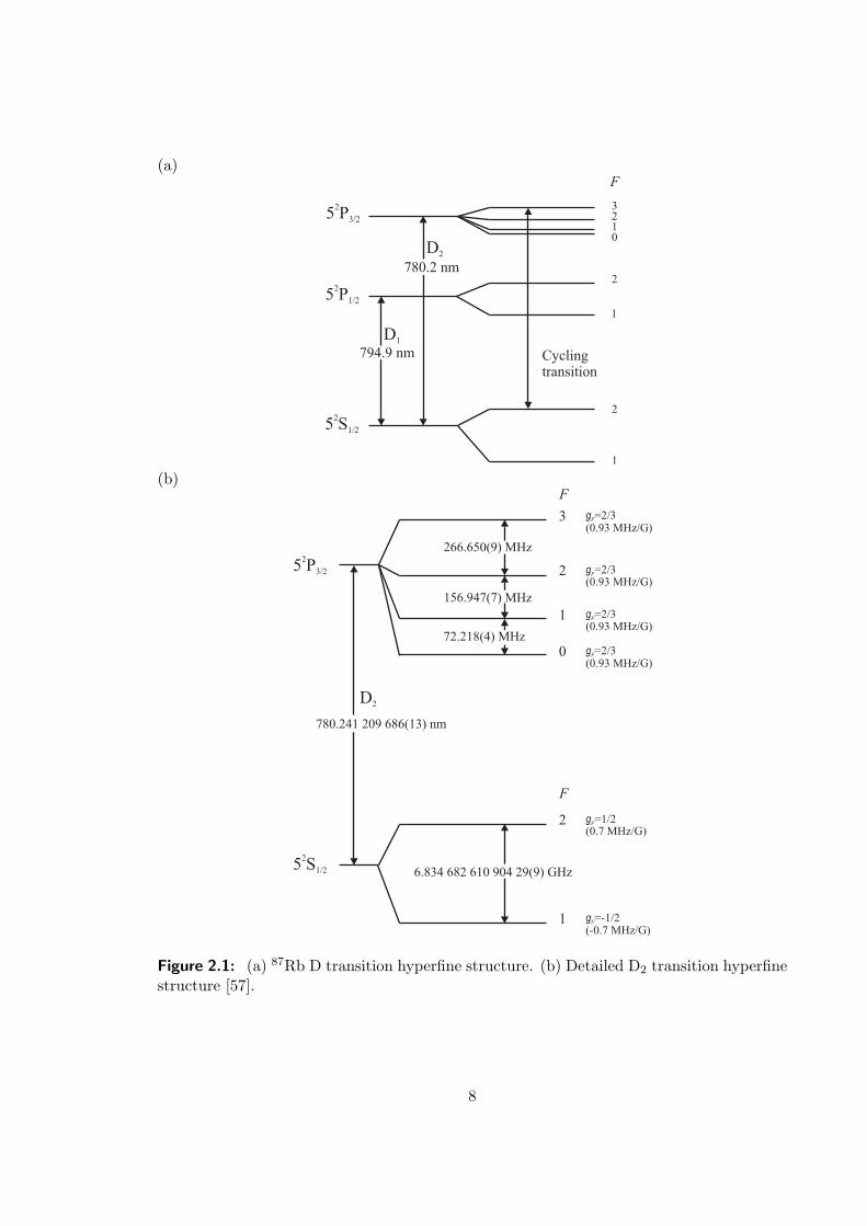
D transitions, i.e., the D1 and D2 lines. The ground and first excited hyperfine structures

and the optical transitions of 87Rb are illustrated in Fig. 2.1(a). The D2 transitions are

used for laser cooling and for probing in this thesis, and the precise frequencies of hyperfine

splitting and the D2 transition wavelength are given in the Fig. 2.1(b).

In each F state, there are 2F + 1 Zeeman sublevels, labeled as mF = F, F − 1, · · · ,−F .

The selection rules for the electric dipole S ↔ P optical transitions are ∆F, ∆mF = 0,±1,

except for mF = 0 ↔ mF ′ = 0 when ∆F = 0. These selection rules allow the 52S1/2,

|F = 2,mF = ±2〉 and 52P3/2, |F = 3,mF = ±3〉 states (shorthand: |F = 2, mF = ±2〉 and

|F ′ = 3,mF ′ = ±3〉) to form closed two-level systems. In addition, the optical transitions

between F = 2 and F ′ = 3 refers to the cycling transitions (see Fig. 2.1(a)). These

transitions are very important because they enable an atom to repeatedly scatter photons

from a laser beam tuned to this transition frequency, which is the key for efficient laser

cooling.

The degeneracy of the mF states is lifted in the presence of a magnetic field. The

magnetic energy shift, or Zeeman shift, of each mF state can be calculated using the Breit-

Rabi formula [58], and for the three mF (1, 0, -1) states in the ground F = 1 manifold they

are given as

E1 = −Ehfs

8− gIµIB − 1

2Ehfs

√1 + x + x2

E0 = −Ehfs

8− 1

2Ehfs

√1 + x2

E−1 = −Ehfs

8+ gIµIB − 1

2Ehfs

√1− x + x2, (2.1)

where

x =gIµIB + gJµBB

Ehfs.

Here Ehfs is the hyperfine splitting, gI and gJ are the Lande g-factor for the nucleus and the

valence electron, µI and µB are the nuclear magnetic moment and the Bohr magneton, and

B is the magnetic field. Since gIµI ¿ gJµB, gIµI is often neglected and x ' gJµBB/Ehfs.

The atomic parameters for 87Rb are given in Appendix A, and the energy shift of ground

7

(a)

5 P2

3/2

5 P2

1/2

5 S2

1/2

F

3210

2

1

2

1

D2

D1

Cyclingtransition

780.2 nm

794.9 nm

(b)

5 P2

3/2

5 S2

1/2

2

1

F

2

1

0

780.241 209 686(13) nm

6.834 682 610 904 29(9) GHz

72.218(4) MHz

156.947(7) MHz

266.650(9) MHz

gF=2/3

gF=2/3

gF=2/3

gF=2/3

gF=1/2

gF=-1/2

3

F

(0.93 MHz/G)

(0.93 MHz/G)

(0.93 MHz/G)

(0.93 MHz/G)

(0.7 MHz/G)

(-0.7 MHz/G)

D2

Figure 2.1: (a) 87Rb D transition hyperfine structure. (b) Detailed D2 transition hyperfinestructure [57].

8

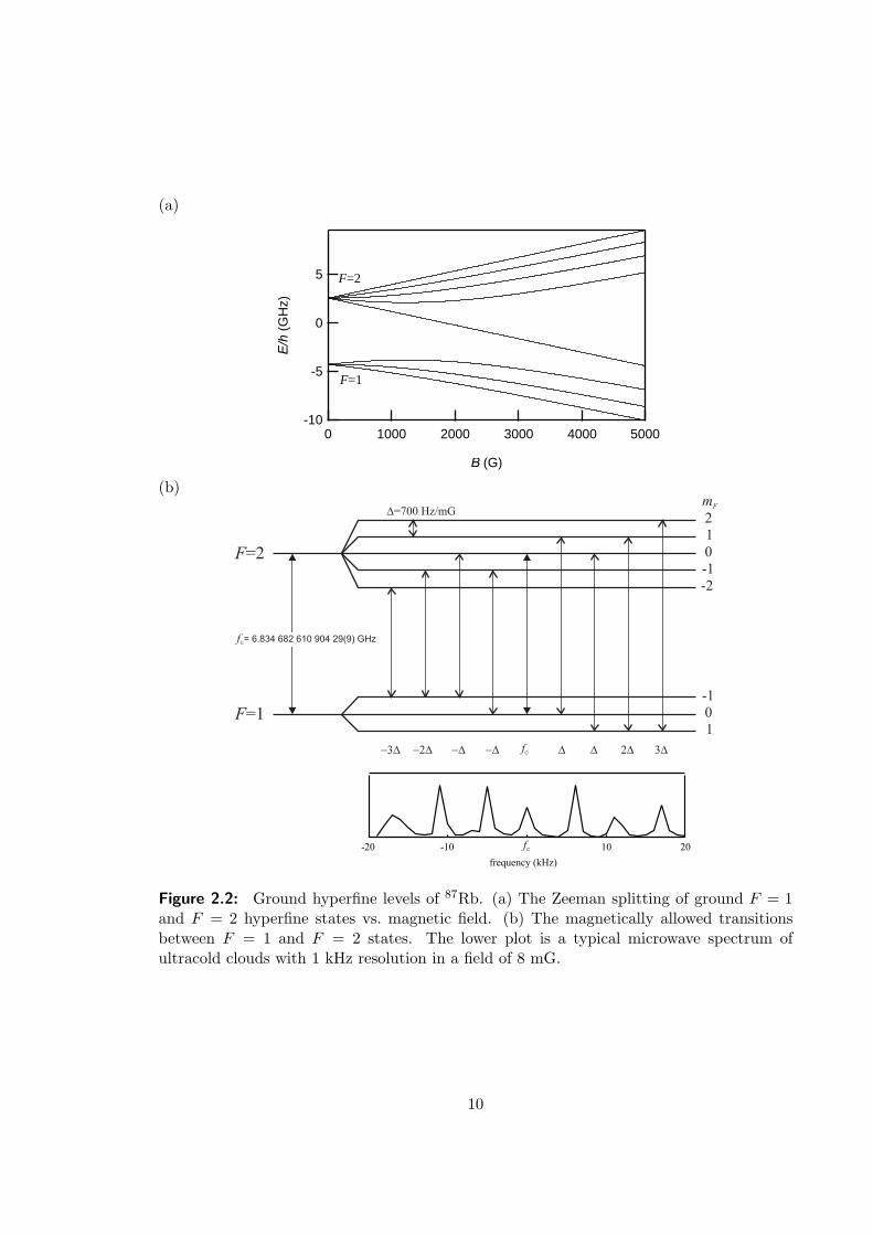
hyperfine states vs. magnetic field is plotted in Fig. 2.2(a). In the low fields, the energy

splitting between two adjacent mF states is ∼ 0.7 MHz/G.

In the studies of spinor condensates, we have used microwaves tuned to the ground state

hyperfine transitions to measure and zero the magnetic fields in the optical traps and to

manipulate the internal spin states of the condensates. The allowed magnetic transitions

between the F = 1 and F = 2 states and a typical microwave spectrum are shown in Fig.

2.2(b).

2.2 Magneto-Optical Trap

The magneto-optical trap (MOT), based on laser cooling, has provided an efficient and

straightforward way to capture and cool millions of atoms to the micro-Kelvin regime.

Since its invention in 1987 [6], magneto-optical trapping has become the workhorse for

modern ultracold atomic physics in the micro-Kelvin regime.

The first atomic Bose-Einstein condensates were achieved using the alkali species: 87Rb,

7Li, and 23Na. Between 1995 and 2003 all of the stable alkali bosonic isotopes and many of

the fermionic isotopes have been cooled to quantum degeneracy. A very important reason

for this success is that alkali atoms exhibit strong optical cycling transitions as noted in the

last section, which enable efficient laser cooling to the µK regime. In BEC experiments, the

MOT provides an increase in the phase space density (PSD) by a factor of over 109 from

ambient conditions and provides favorable initial conditions for subsequent evaporation to

quantum degeneracy.

The standard MOT consists of three orthogonal pairs of counter-propagating circularly

polarized laser beams and a pair of anti-Hemholtz coils. The lasers are tuned to the red of

the cycling transition by a few atomic linewidths for Doppler laser cooling [6]. The anti-

Hemholtz coils (MOT coils) create a spatially varying Zeeman shift for the laser cooled

atoms. The combination of the MOT coils and cooling lasers creates a spatial-dependent

and velocity dependent radiation pressure that provide both a restoring and viscous force

for the atoms.

The trap depth of a typical MOT is only ∼ 1 mK. If it is used to directly capture atoms

9

(a)

-10

-5

0

5E

/h (

GH

z)

500040003000200010000

B (G)

F=2

F=1

(b)

F=2

F=1

D D 2D 3D-3D -2D -D -D fc

D=700 Hz/mG

fc= 6.834 682 610 904 29(9) GHz

mF

2

1

0

-1

-2

-1

0

1

-20 -10 10 20

frequency (kHz)

fc

Figure 2.2: Ground hyperfine levels of 87Rb. (a) The Zeeman splitting of ground F = 1and F = 2 hyperfine states vs. magnetic field. (b) The magnetically allowed transitionsbetween F = 1 and F = 2 states. The lower plot is a typical microwave spectrum ofultracold clouds with 1 kHz resolution in a field of 8 mG.

10

from a vapor at 300 K, it can only capture the atoms in the low velocity tail of the Boltzmann

distribution. To enhance the capture efficiency of the MOT, various enhancement techniques

have been developed. These include a Zeeman slower to increase the brightness of the atomic

bream, and a double MOT system to transfer a MOT from a high pressure chamber to a

low pressure chamber. In our experiment, neither of these two techniques is necessary.

Thorough information of laser cooling and the MOT can be found in ref. [59].

2.2.1 Diode Lasers

One advantage of working with rubidium is that one can find inexpensive high-power single

mode laser diodes and diode amplifier chips delivering up to 1 W at 780 nm. In addition,

diodes lasers are compact, long lasting, and almost maintenance-free following initial setup.

Furthermore, the laser linewidth can be easily reduced to below 1 MHz and locked to atomic

transitions following well established techniques [60, 61, 62].

In this thesis, some of the experiments were done with homemade diode lasers. Lately,

1 W tapered diode amplifiers have become available, and we have recently used these

amplifiers in our experiments.

The cooling lasers (MOT lasers) are tuned to the F = 2 ↔ F ′ = 3 transition of 87Rb.

Each laser beam is circularly polarized to favor σ± transitions (∆m = ±1). Although the

MOT laser frequency is tuned close to the F = 2 ↔ F ′ = 3 transition, there is a small

probability that the atoms can be excited to the F ′ = 2 state, which can spontaneously

decay to the F = 1 ground state. Due to the large ground state hyperfine splitting, atoms

in the F = 1 state are decoupled from the cooling light. To repump these atoms, a second

laser resonant with the F = 1 ↔ F ′ = 2 transition is added to optically pump the atoms

back to the F = 2 state — this is referred to as the repump laser.

The experiment requires up to four MOT lasers and one repump laser. As shown in

Fig. 2.5 we use a master-slave configuration for the MOT lasers. An external-cavity diode

laser (ECDL) serving as a master laser is frequency stabilized to an atomic transition of Rb.

The output of the master laser is frequency shifted by a frequency tunable acousto-optic

modulator (AOM), and then seeds three slave lasers. Each slave laser is sent through an

11

AOM to provide control of the optical power and then coupled into a single-mode, polariza-

tion maintaining optical fiber. After exiting the fiber, each beam is expanded, collimated,

and then directed into the vacuum chamber through anti-reflection coated viewports. The

typical power at the fiber output is 20 ∼ 40 mW, and the 1/e2 radius of each MOT beam

is 12.5 mm. The repump laser is combined with one slave laser and then coupled into the

same fiber. The repump power at the fiber output is 12 mW. The six MOT beams are

formed by retro-reflecting the three MOT beams.

2.2.2 Laser Frequency Stabilization and Tuning

The diode lasers are first stabilized by controlling the temperature and diode current [63,

64, 65] with homemade temperature servo system and current controllers. The linewidth

of master laser is then reduced to below 1 MHz by an external cavity, formed with an

1800 lines/mm grating in the Littrow configuration. The cavity length is controlled by a

piezo-electric actuator (PZT). The master laser is locked to a Doppler-free atomic absorption

signal obtained from a standard saturated absorption setup. The laser frequency is stabilized

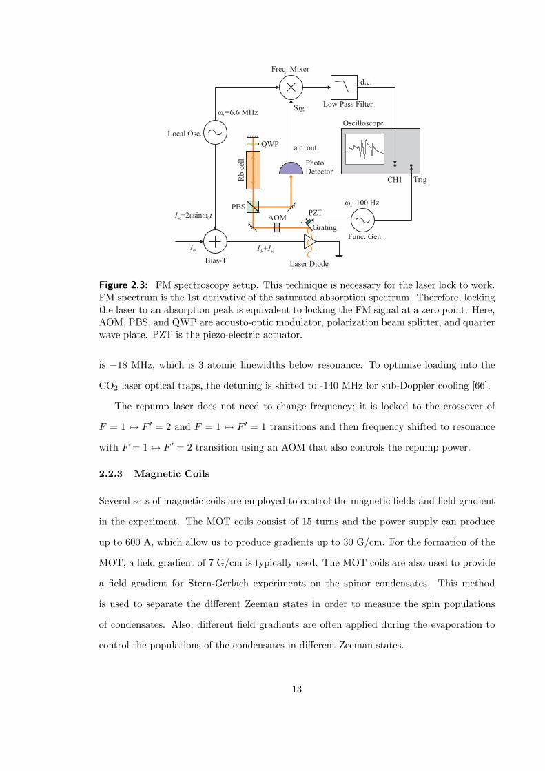
to an absorption peak using frequency modulation (FM) spectroscopy by locking it to a zero

crossing point of the FM signal using a PI (proportional-integral) circuit. The setup for the

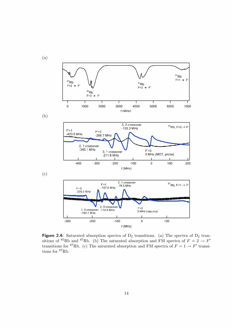
FM spectroscopy is shown in Fig. 2.3, and the saturated absorption spectra and FM signal

of 87Rb D2 transitions are shown in Fig. 2.4.

Doppler laser cooling requires the cooling lasers to be frequency stabilized to the red

of the cycling transition. In the experiment, the master laser frequency is locked to the

crossover of F = 2 ↔ F ′ = 3 and F = 2 ↔ F ′ = 1 transitions, which is −211.8 MHz below

the cycling transition (see Fig. 2.4). To change the detuning between the MOT lasers and

the cycling transition, the master laser output is shifted using a frequency tunable AOM.

This AOM is configured in a double-pass configuration and the output laser beam of the

AOM is then used to injection lock three slave lasers. The layout of the diode lasers is

shown in Fig. 2.5. The frequency of the MOT beams can be changed from -180 MHz to

+20 MHz relative to the cycling transition within < 100 µs. This detuning range allows us

to achieve sub-Doppler cooling in the final stage of the MOT. The typical MOT detuning

12

w0=6.6 MHz

Local Osc.

Sig.

I tac=2 sine w0

Idc I Idc ac+R

b c

ell

Low Pass Filter

d.c.

Grating

PZT

QWP

ws~100 Hz

TrigCH1

Oscilloscope

a.c. out

AOM

PhotoDetector

Bias-T

Freq. Mixer

Laser Diode

Func. Gen.

PBS

Figure 2.3: FM spectroscopy setup. This technique is necessary for the laser lock to work.FM spectrum is the 1st derivative of the saturated absorption spectrum. Therefore, lockingthe laser to an absorption peak is equivalent to locking the FM signal at a zero point. Here,AOM, PBS, and QWP are acousto-optic modulator, polarization beam splitter, and quarterwave plate. PZT is the piezo-electric actuator.

is −18 MHz, which is 3 atomic linewidths below resonance. To optimize loading into the

CO2 laser optical traps, the detuning is shifted to -140 MHz for sub-Doppler cooling [66].

The repump laser does not need to change frequency; it is locked to the crossover of

F = 1 ↔ F ′ = 2 and F = 1 ↔ F ′ = 1 transitions and then frequency shifted to resonance

with F = 1 ↔ F ′ = 2 transition using an AOM that also controls the repump power.

2.2.3 Magnetic Coils

Several sets of magnetic coils are employed to control the magnetic fields and field gradient

in the experiment. The MOT coils consist of 15 turns and the power supply can produce

up to 600 A, which allow us to produce gradients up to 30 G/cm. For the formation of the

MOT, a field gradient of 7 G/cm is typically used. The MOT coils are also used to provide

a field gradient for Stern-Gerlach experiments on the spinor condensates. This method

is used to separate the different Zeeman states in order to measure the spin populations

of condensates. Also, different field gradients are often applied during the evaporation to

control the populations of the condensates in different Zeeman states.

13

(a)

70006000500040003000200010000

f (MHz)

87Rb

F=2 F'

85Rb

F=3 F'

85Rb

F=2 F'

87Rb

F=1 F'

(b)

-400 -300 -200 -100 0 100 200

f (MHz)

87Rb, F=2 -> F'

F'=30 MHz (MOT, probe)

3, 2 crossover-133.3 MHz

3, 1 crossover-211.8 MHz

F'=2-266.7 MHz

F'=1-423.6 MHz

2, 1 crossover-345.1 MHz

(c)

-300 -200 -100 0 100

f (MHz)

87Rb, F=1 -> F'

F'=20 MHz (repump)

2, 1 crossover-78.5 MHz

2, 0 crossover-114.6 MHz

F'=1-157.0 MHz

1, 0 crossover-193.1 MHz

F'=0-229.2 MHz

Figure 2.4: Saturated absorption spectra of D2 transitions. (a) The spectra of D2 tran-sitions of 85Rb and 87Rb. (b) The saturated absorption and FM spectra of F = 2 → F ′

transitions for 87Rb. (c) The saturated absorption and FM spectra of F = 1 → F ′ transi-tions for 87Rb.

14

RP M S1 S2 S3

Optical fiber with coupler

Rb vapor cell

Polarization beam splitter (PBS)

Photo detector (PD)

Optical flat

Amorphous prism pair

Faraday isolator

Acousto-optical modulator (AOM)

Half wave plate (HWP)

Quarter wave plate (QWP)

w =w +2wref M 1

wM w =w +2w

s M 2w =w +2w

s M 2w =w +2w

s M 2

w1

w2

w3

w3

w3

FL=5”

AOM1

AOM2

AOM3 AOM3 AOM3

RPAOM

FL=1”

FL=2”

shutter

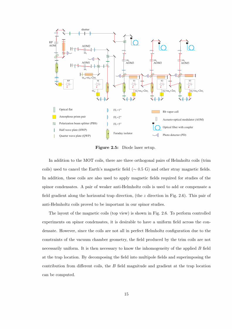
Figure 2.5: Diode laser setup.

In addition to the MOT coils, there are three orthogonal pairs of Helmholtz coils (trim

coils) used to cancel the Earth’s magnetic field (∼ 0.5 G) and other stray magnetic fields.

In addition, these coils are also used to apply magnetic fields required for studies of the

spinor condensates. A pair of weaker anti-Helmholtz coils is used to add or compensate a

field gradient along the horizontal trap direction, (the z direction in Fig. 2.6). This pair of

anti-Helmholtz coils proved to be important in our spinor studies.

The layout of the magnetic coils (top view) is shown in Fig. 2.6. To perform controlled

experiments on spinor condensates, it is desirable to have a uniform field across the con-

densate. However, since the coils are not all in perfect Helmholtz configuration due to the

constraints of the vacuum chamber geometry, the field produced by the trim coils are not

necessarily uniform. It is then necessary to know the inhomogeneity of the applied B field

at the trap location. By decomposing the field into multipole fields and superimposing the

contribution from different coils, the B field magnitude and gradient at the trap location

can be computed.

15

Vacuum chamber

Trim 2, 14 turns= 1.5”, = 5”D d

Trim 3, 14 turns= 4.5”, = 1.9”D d

New Trim 1, 40 turns= 3.55”, = 12.5”D d

MOT coils, 15 turns= 4.5”, = 8”D d

Gradient coils, 5 turns= 4.5”, = 1.9”D d

xy

z

Figure 2.6: Top view of the Helmholtz (bias) and anti-Helmholtz (gradient) coils. Thearrows represent the direction of the electric current of the coils. In this case, the diameterof each pair of coils is D, and separation between the two coils is d.

16

The multipole expansion (around the center) for a scalar magnetic potential of a circular

Helmholtz coil is [67]

ψ(r, θ) = −µ0NI∞∑

n=odd

1n

(r

a

)nsin θ0P

1n(cos θ0)Pn(cos θ), r < a . (2.2)

Here N and I are the number of winding turns and the electrical current, and a and θ0 are

defined in Fig. 2.7. Pn(cos θ) are the Legendre polynomials, and P 1n(cos θ) = − d

dθPn(cos θ)

are the associated Legendre polynomials. The magnetic field is B(r, θ) = −∇ψ(r, θ), and

Br(r, θ) = −µ0NI∞∑

n=odd

rn−1

ansin θ0 P 1

n(cos θ0)Pn(cos θ) , (2.3a)

Bθ(r, θ) = −µ0NI∞∑

n=odd

1n

rn−1

ansin θ0P

1n(cos θ0)P 1

n(cos θ) . (2.3b)

With these expressions, together with a transformation to Cartesian coordinates, the mag-

netic fields and curvatures are readily found in different directions. Note that for symmetric

coils, the magnetic field gradient of each pair of coils is cancelled. In our setup, the field

curvature along the x direction is B′′x = 40 mG/cm2 per Gauss of field produced along x

direction. Similarly, B′′y = 245 and B′′

z = 19 mG/cm2 for 1 G of field applied along the

y, z direction, respectively. The x, y, z directions are defined in Fig. 2.6 . It is noted that

the Trim 2 coil has the largest field inhomogeneity (B′′y ) since it is furthest from the ideal

Helmholtz (d = D/2) geometry. Given the maximum fields we generated using different

coils, and the trap position uncertainty of 1 mm with respect to the center of the coils, the

estimated maximum field gradients are B′x ' B′′

xx ≤ 20 mG/cm at 1 G along x direction,

B′y ' B′′

yy ≤ 15 mG/cm at 0.5 G along y direction, and B′z ' B′′

z z ≤ 5mG/cm at 0.5 G

along z direction.

2.3 Vacuum Chamber and Atom Source

An ultra-high vacuum environment is required for BEC experiments in order to isolate the

trapped ultracold atoms from collisions with fast room temperature atoms. The pressure in

our vacuum chamber is between low 10−10 and high 10−11 torr, which results in a vacuum

limited lifetime of 10 s [68]. This is sufficient for our experiments since evaporative cooling

takes less than 2 s due to the fast collision dynamics in our optical traps. The lifetime

17

aq0

z

R

d/2

NI

NI

Figure 2.7: A side view of a Helmholtz coil (not necessary in perfect geometry).

of our condensates is 3 − 5 sec, which is not limited by the vacuum but by three-body

recombination loss.

We use 87Rb in our BEC experiments, which is a metallic solid at room temperature.

An ampule of rubidium metal is placed in a flexible bellows connected to the main chamber.

This port is aligned in direct line of sight with the MOT. The vapor pressure of rubidium

at room temperature is ∼ 2×10−7 torr, and the vapor contains 27.8% of 87Rb and 72.2% of

85Rb by natural abundance. The atoms diffuse from the source to the main chamber when

the valve between the two chambers is opened.

2.4 Optical Dipole Force Trap

Optical dipole force traps are important tools in our BEC experiments. The laser cooled

atoms are loaded into the optical trap from which we perform forced evaporation to achieve

quantum degeneracy. Optical traps offer higher restoring forces than typical magnetic traps,

which leads to higher atomic density for efficient evaporation. Optical trapping of neutral

atoms was first observed in 1986 [69], and evaporative cooling in a crossed optical trap was

first demonstrated in 1994 [70].

The optical dipole force comes from the dispersive interaction of the intensity gradient

of the light field with the atomic dipole moment which is induced by the optical field. The

dipole moment induced by the field is given by ~p = α~E, where α is the complex frequency

dependent atomic polarizability. The interaction potential of the induced dipole moment

18

in the driving field is given by

U = −〈∫

~p · d ~E〉 = −12〈~p · ~E〉 = − 1

2ε0cRe(α)I, (2.4)

where I is the light intensity. Here the angular brackets represent a time average over the

oscillation period of the driving optical field. The averaged optical power dissipated by the

atoms is given by

Pabs = 〈~p · ~E〉 =ω

ε0cIm(α)I. (2.5)

where ω is the angular frequency of the light field. The corresponding photon scattering

rate is

Γsc =Pabs

~ω. (2.6)

The polarizability α can be estimated using a simple Lorentz model, x+Γωx+ω20 = − e

mE(t),

where the classical damping rate Γω is due to radiative energy loss and is given by the Larmor

formula, Γω = e2ω2/6πε0mec3. Solving the equation of motion, the polarizability is found

as

α = 6πε0c3 Γ/ω2

0

ω20 − ω2 − i(ω3/ω2

0)Γ. (2.7)

Here Γω is replaced with the on-resonance damping rate Γ with Γω = (ω0/ω)2Γ. The on-

resonance damping rate can also be determined by the dipole transition in the semi-classical

model, in which an atom is treated quantum mechanically, while the driving optical field is

treated classically. Then the damping rate is given as

Γ =ω3

0

3πε0~c3|〈e|p|g〉|2, (2.8)

where 〈e|p|g〉 is the dipole transition matrix element.

When the detuning is large and saturation effects can be neglected, the trapping poten-

tial and scattering rate can be approximated as

U(r) = −3πc2

2ω30

(Γ

ω0 − ω+

Γω0 + ω

)I(r), (2.9)

Γsc(r) =3πc2

2~ω30

(ω

ω0)3

(Γ

ω0 − ω+

Γω0 + ω

)2

I(r). (2.10)

19

In a case of a typical far-off resonance trap (FORT), in which the detuning |∆| = |ω−ω0| ¿ω0, Eq. (2.9) and (2.10) can be further reduced to

U(r) = −3πc2

2ω30

Γ∆

I(r), (2.11)

Γsc =3πc2

2~ω30

(Γ∆

)2

I(r) =Γ~∆

U(r). (2.12)

It is easily seen while keeping the same trap depth, the scattering rate can be greatly reduced

by increasing the detuning. In an extreme case where ω ¿ ω0, such as the case of CO2

laser, the condition |∆| ¿ ω0 no longer holds. Eq. (2.9) and (2.10) should be reduced to

U(r) ' −3πc2Γω4

0

I(r) = − αs

2ε0cI(r), (2.13)

Γsc =2Γ~ω0

(ω

ω0

)3

U(r). (2.14)

Here αs is the static polarizability. In this case, the optical trap is a quasi electrostatic trap

(QUEST) [71], and the scattering rate is reduced so much that it is essentially a conservative

trap. Take for example, a typical trap depth of 100 µK for a CO2 laser dipole force trap,

the scattering rate is only 1.1 photon per atom per hour for 87Rb ! A more detail descussion

of optical dipole traps can be found in ref. [72].

The dipole force trapping beams are generated from two CO2 gas lasers (Synrad 48-1

and DEOS LC-100NV), with wavelength, λ = 10.6 µm. The beams are tightly focused

with f = 38 mm focal length, ZeSn aspherical lenses inside the chamber. There are six

lenses inside the chamber forming three orthogonal 1:1 telescopes that allow us to create

a wide range of travelling wave and standing wave configurations including a 6 beam 3-D

optical lattice. For the condensate work, two crossed lasers either in travelling wave or

optical lattice configurations are used, intersected at right angles; one beam is oriented in

the horizontal direction and one beam is inclined at 45 from the vertical direction. Each

beam passes through a germanium AOM to provide independent control of the power in the

two beams. Additionally, the beams are frequency shifted 80 MHz relative to each other

so that any spatial interference patterns between the two beams are time-averaged to zero

[73]. The layout of our CO2 laser beams are provided in Fig. 2.8, and the radio frequency

(RF) source for each AOM is given in Fig. 2.9.

20

AOM1

AOM2

50/50 BS

pinhole: 200 mm

pinhole: 200 mm

HeNe

Synra

d 4

8-1

DE

OS

LC

-100N

V

AOM3

Chamber

kineticmount

motorizedtranslationstage

Figure 2.8: Setup of our CO2 dipole force trap. The pinholes shown here are optional. Themodel number of AOM1 and AOM2 is Isomet 1207B-6, and that of AOM3 is IntraActionAGM-4010BJ1. Additionally, the model number of the motorized translation stage and itscontroller are Newport UTM50PP1HL and ESP300, respectively.

21

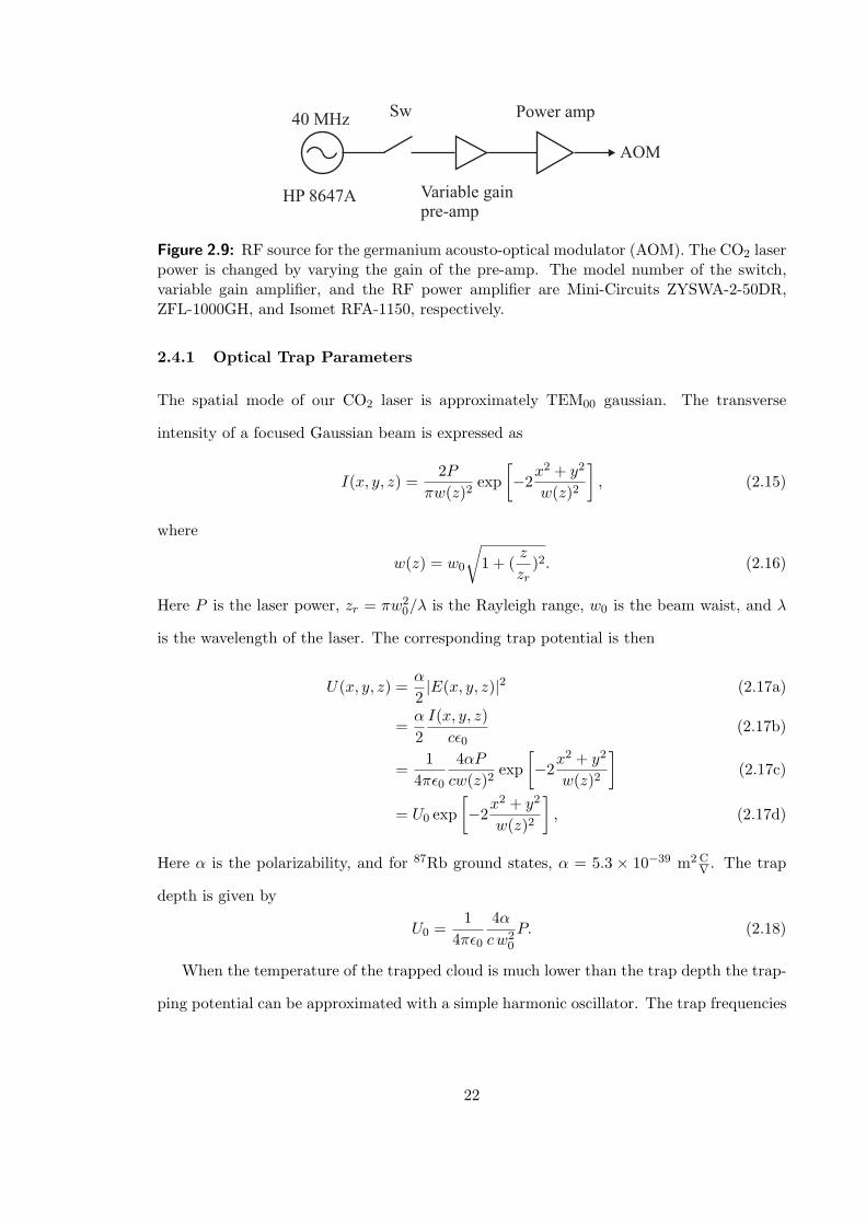
40 MHzSw

HP 8647A

AOM

Variable gainpre-amp

Power amp

Figure 2.9: RF source for the germanium acousto-optical modulator (AOM). The CO2 laserpower is changed by varying the gain of the pre-amp. The model number of the switch,variable gain amplifier, and the RF power amplifier are Mini-Circuits ZYSWA-2-50DR,ZFL-1000GH, and Isomet RFA-1150, respectively.

2.4.1 Optical Trap Parameters

The spatial mode of our CO2 laser is approximately TEM00 gaussian. The transverse

intensity of a focused Gaussian beam is expressed as

I(x, y, z) =2P

πw(z)2exp

[−2

x2 + y2

w(z)2

], (2.15)

where

w(z) = w0

√1 + (

z

zr)2. (2.16)

Here P is the laser power, zr = πw20/λ is the Rayleigh range, w0 is the beam waist, and λ

is the wavelength of the laser. The corresponding trap potential is then

U(x, y, z) =α

2|E(x, y, z)|2 (2.17a)

=α

2I(x, y, z)

cε0(2.17b)

=1

4πε0

4αP

cw(z)2exp

[−2

x2 + y2

w(z)2

](2.17c)

= U0 exp[−2

x2 + y2

w(z)2

], (2.17d)

Here α is the polarizability, and for 87Rb ground states, α = 5.3 × 10−39 m2 CV . The trap

depth is given by

U0 =1

4πε0

4α

cw20

P. (2.18)

When the temperature of the trapped cloud is much lower than the trap depth the trap-

ping potential can be approximated with a simple harmonic oscillator. The trap frequencies

22

Cross trap 1-D latticeSingle focus

x

y z

Figure 2.10: Three trap geometries.

Table 2.1: Table of trap frequencies. Here w(z) = w0

√1 + ( z

zr)2, zr = πw2

0/λ, k = 2π/λ,

and U0 = 14πε0

4αcw2

0P , where P is the power per beam. We assume that the laser beams have

the same circular Gaussian profile and the same power.

Trap Parameters Single focus Cross trap 1D lattice

Potential U01+( z

zr)2

e− 2r2

w(z)2 U01+( z

zr)2

e− 2(x2+y2)

w(z)2 4U01+( z

zr)2

e− 2r2

w(z)2 cos2 kz

+ U01+( x

zr)2

e− 2(y2+z2)

w(x)2

Trap Depth U0 2U0 4U0

Low Frequency (ωL)√

2U0mz2

r

√4U0

mw20

√16U0

mw20

High Frequency (ωH)√

4U0

mw20

√8U0

mw20

√8U0k2

m

Mean Frequency (ω) (ω2LωH)1/3 (ω2

LωH)1/3 (ω2LωH)1/3

Aspect Ratio (ωH/ωL)√

2πw0λ

√2

√2πw0λ

can be measured using parametric resonance method, and they can be easily computed using

ωri =[−1

m

∂2U(x, y, z)∂r2

i

]1/2

(x,y,z)=(0, 0, 0)

, (2.19)

where ri = x, y, z, and m is the mass of the atom.

By superimposing more than one focused Gaussian beams, one can create optical po-

tentials with a variety of trap geometries. In this thesis, the single focused, cross trap, and

1D lattice geometries are mainly used in the BEC experiments, and they are illustrated in

Fig. 2.10. Some useful trap parameters for these traps are listed in Table 2.1 for reference.

23

(a)

CCDchip

Atomiccloud

MOT laser

(b)

CCDchip

Atomiccloud

probe laser

Figure 2.11: Schematic of probe techniques. (a) Fluorescence imaging. (b) Absorptionimaging.

2.5 Atom Probe and Signal Collection

The atomic cloud is measured using either fluorescence or absorption imaging techniques.

There are two imaging systems that view from the side and the top of the trap. A 1:1 imaging

system is used to view from the side and the image is recorded by a surveillance charge-

coupled device (CCD) camera. A 4:1 imaging system is used to view from the top using a

cooled scientific CCD camera. For fluorescence probing, we pulse on all of the MOT beams

at the maximum power of 35 mW/cm2 for 100 µs, which is equivalent to a total intensity of

45Is, where Is = 1.6 mW/cm2 is saturation intensity. The fluorescent images are taken with

both cameras. For absorption imaging, a vertical, weak probe laser beam is sent through

the trapped atoms and directed through the imaging optics to the cooled CCD camera. The

probe laser is pulsed on for 100 µs at an intensity of 1 mW/cm2. For both techniques, the

laser frequency and polarization are tuned to drive the |F = 2,mF = 2〉 → |F ′ = 3,mF = 3〉transition. To image the atoms in the F = 1 state, the repump laser is also pulsed during

imaging. The probe techniques are illustrated in Fig. 2.11, and the theory of imaging

techniques and quantitative imaging analysis will be given in the next chapter.

24

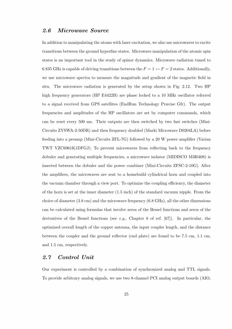
2.6 Microwave Source

In addition to manipulating the atoms with laser excitation, we also use microwaves to excite

transitions between the ground hyperfine states. Microwave manipulation of the atomic spin

states is an important tool in the study of spinor dynamics. Microwave radiation tuned to

6.835 GHz is capable of driving transitions between the F = 1 ↔ F = 2 states. Additionally,

we use microwave spectra to measure the magnitude and gradient of the magnetic field in

situ. The microwave radiation is generated by the setup shown in Fig. 2.12. Two HP

high frequency generators (HP E4422B) are phase locked to a 10 MHz oscillator referred

to a signal received from GPS satellites (EndRun Technology Præcise Gfr). The output

frequencies and amplitudes of the HP oscillators are set by computer commands, which

can be reset every 500 ms. Their outputs are then switched by two fast switches (Mini-

Circuits ZYSWA-2-50DR) and then frequency doubled (Marki Microwave D0204LA) before

feeding into a preamp (Mini-Circuits ZFL-7G) followed by a 20 W power amplifier (Varian

TWT VZC6961K1DFGJ). To prevent microwaves from reflecting back to the frequency

dobuler and generating multiple frequencies, a microwave isolator (MIDISCO M3I0408) is

inserted between the dobuler and the power combiner (Mini-Circuits ZFSC-2-10G). After

the amplifiers, the microwaves are sent to a homebuild cylindrical horn and coupled into

the vacuum chamber through a view port. To optimize the coupling efficiency, the diameter

of the horn is set at the inner diameter (1.5 inch) of the standard vacuum nipple. From the

choice of diameter (3.8 cm) and the microwave frequency (6.8 GHz), all the other dimensions

can be calculated using formulas that involve zeros of the Bessel functions and zeros of the

derivatives of the Bessel functions (see e.g., Chapter 8 of ref. [67]). In particular, the

optimized overall length of the copper antenna, the input coupler length, and the distance

between the coupler and the ground reflector (end plate) are found to be 7.5 cm, 1.1 cm,

and 1.5 cm, respectively.

2.7 Control Unit

Our experiment is controlled by a combination of synchronized analog and TTL signals.

To provide arbitrary analog signals, we use two 8-channel PCI analog output boards (AIO,

25

10 MHz 3.417 GHz

x2 +

Isolator

Sw1

Sw2

GPSHP 4422B

Horn

Freq.doubler

x2

3.417 GHz

Figure 2.12: Microwave setup. The frequencies and amplitudes of two HP oscillators are setby computer commands. The two switches, Sw1 and Sw2, are controlled by two independentdigital signals.

National Instrument 6713) which are controlled by LabView programs (VIs). The TTL

signals are mostly generated by TTL pulse generators (SRS DG535 and BNC 500) which

are triggered by AIO outputs. Recently, we have replaced most of the TTL pulse generators

with a 32-channel PCI digital input/output board (DIO, model number NI-6534). For TTL

pulses shorter than 100 µs, high precision pulse generators (SRS-DG535) are still employed.

26

CHAPTER III

DETECTION AND IMAGE ANALYSIS FOR

ULTRACOLD ATOMIC CLOUDS

Trapped ultracold clouds are small, typically only 10’s of microns across, and they are

isolated in a ultrahigh vacuum chamber. As such, it is not feasible to interrogate the

trapped atoms with material probes, such as a thermometer 1. Laser cooling and magneto-

optical trapping rely on the strong interaction of atoms with a near-resonant light. These

same interactions are also used to detect atoms and measure dynamical quantities of the

atom clouds.

Probing of an ultracold cloud is straightforward via measurements of the optical power

radiated from or transmitted through the atomic cloud. These two types of probing tech-

niques are referred to as fluorescence and absorption spectroscopies, respectively. Imaging

the radiation on a camera allows measurement of the ensemble properties, such as the

spatial and momentum distributions of the atomic cloud. Image analysis for an ultracold

atomic cloud is also straightforward, since a trapped ultracold atomic cloud is a very simple

and clean system such that its properties can be understood from first principles.

A trapped Bose gas at thermal equilibrium is described by a Boltzmann distribution

when the temperature is much higher than the BEC critical temperature, and a Bose

distribution when the temperature is close to the critical temperature. At temperatures

much lower than the critical temperature, when the trapped cloud contains mostly a Bose-

Einstein condensate, its ground state properties and dynamics are well-described by the

nonlinear Schrodinger equation, or Gross-Pitaevskii equation.

In this chapter, we present the techniques employed to determine the atomic properties

from measured images of the atom clouds. In addition, we present how to extract physical

1While material probes such as a multichannel plate can be used to detect atoms [74], optical probes aregenerally simpler and more versatile.

27

quantities from the acquired images, and how one can derive other physical quantities from

these measurements using simple statistical mechanics formula.

3.1 Measurement Techniques for Ultracold Atoms

The atomic clouds are measured using both fluorescence and absorption imaging techniques.

The images are recorded with charge-coupled device (CCD) cameras and then downloaded

to the computer for subsequent quantitative analysis.

3.1.1 Fluorescence Imaging

Probing 87Rb atoms is relatively easy due to strength of the cycling transition. In addition,

it is straightforward to interpret and calibrate the fluorescence signals using a two-level

atom model. The photon scattering rate for a two-level atom is given by

γp =γ

2s0

1 + s0 + (2∆/γ)2, (3.1)

where s0, γ, and ∆ are the saturation parameter, spontaneous decay rate, and the laser

detuning from resonance. Here ∆ = ωL − ω0 − ~k · ~v, where ωL and ω0 are the laser and

atomic transition frequencies, and ~k and ~v are the wavevector of the laser and the velocity of

the atom. The term ~k ·~v represents the Doppler shift; for ultracold atoms, this shift is much

smaller than the atomic transition linewidth, and thus can be neglected. The saturation

parameter is defined as

s0 ≡ I/Isat, (3.2)

where I and Isat are the laser intensity and the saturation intensity with

Isat ≡ γ

2hc

λ

1σeg

. (3.3)

Here λ is the atomic transition wavelength, and σeg = 3λ2/2π is the on-resonance absorption

cross section. The numerical values of these quantities for 87Rb are listed in the Table A.1.

The maximum scattering rate for 87Rb cycling transition is γ/2 = π · 5.8× 106 s−1.

Fluorescence signals come from the resonantly scattered photons. To maximize the

strength of the fluorescent signal, laser beams with high saturation parameter are typically

used, and this unavoidably heats the atoms. Assuming that the photons are scattered in

28

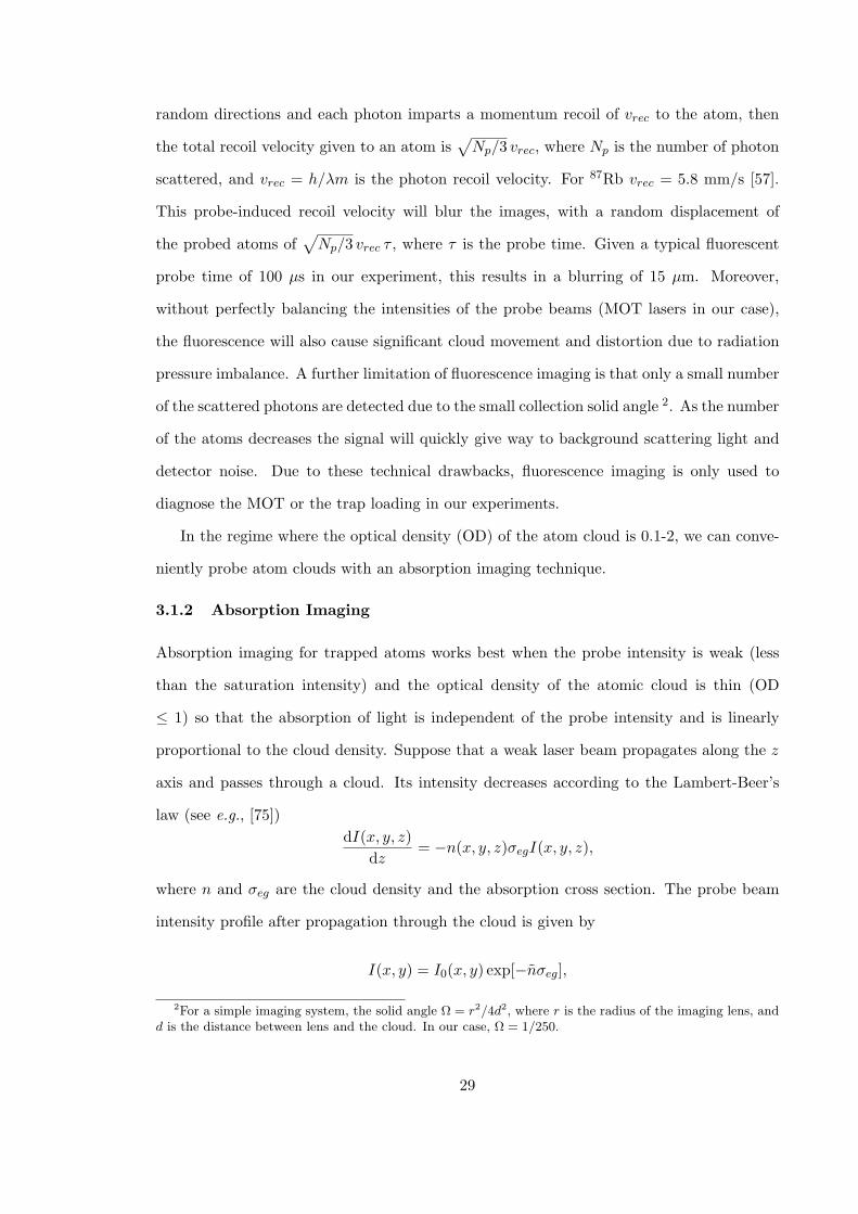
random directions and each photon imparts a momentum recoil of vrec to the atom, then

the total recoil velocity given to an atom is√

Np/3 vrec, where Np is the number of photon

scattered, and vrec = h/λm is the photon recoil velocity. For 87Rb vrec = 5.8 mm/s [57].

This probe-induced recoil velocity will blur the images, with a random displacement of

the probed atoms of√

Np/3 vrec τ , where τ is the probe time. Given a typical fluorescent

probe time of 100 µs in our experiment, this results in a blurring of 15 µm. Moreover,

without perfectly balancing the intensities of the probe beams (MOT lasers in our case),

the fluorescence will also cause significant cloud movement and distortion due to radiation

pressure imbalance. A further limitation of fluorescence imaging is that only a small number

of the scattered photons are detected due to the small collection solid angle 2. As the number

of the atoms decreases the signal will quickly give way to background scattering light and

detector noise. Due to these technical drawbacks, fluorescence imaging is only used to

diagnose the MOT or the trap loading in our experiments.

In the regime where the optical density (OD) of the atom cloud is 0.1-2, we can conve-

niently probe atom clouds with an absorption imaging technique.

3.1.2 Absorption Imaging

Absorption imaging for trapped atoms works best when the probe intensity is weak (less

than the saturation intensity) and the optical density of the atomic cloud is thin (OD

≤ 1) so that the absorption of light is independent of the probe intensity and is linearly

proportional to the cloud density. Suppose that a weak laser beam propagates along the z

axis and passes through a cloud. Its intensity decreases according to the Lambert-Beer’s

law (see e.g., [75])dI(x, y, z)

dz= −n(x, y, z)σegI(x, y, z),

where n and σeg are the cloud density and the absorption cross section. The probe beam

intensity profile after propagation through the cloud is given by

I(x, y) = I0(x, y) exp[−nσeg],

2For a simple imaging system, the solid angle Ω = r2/4d2, where r is the radius of the imaging lens, andd is the distance between lens and the cloud. In our case, Ω = 1/250.

29

where n =∫

n(x, y, z)dz is the column density. The optical density of the cloud at the

location (x, y) is

σegn(x, y) = − lnT (x, y), (3.4)

where T (x, y) is the relative transmission of the beam. The relative transmission can be

measured by comparing the laser beam profiles measured with and without the presence

of atoms. Referring to the measured profiles in the above two conditions as the signal

and reference images and denoting them as S(x, y) and S0(x, y), respectively, the relative

transmission is simply T (x, y) = S(x, y)/S0(x, y). Probe laser profiles are generally recorded

by a CCD camera, and one needs to take a third background image, Sb(x, y), with no probe

beam, and then subtract this background from the signal and the reference images. This

way, contamination from stray scattering light, and any background added by the camera

electronics can be eliminated. Therefore, in practice the recorded optical density is given

by

σegn(x, y) = − lnS(x, y)− Sb(x, y)S0(x, y)− Sb(x, y)

= − lnT (x, y). (3.5)

The advantage of this technique is that, since the absorption imaging measures the

relative transmission of the laser beam with and without the presence of atoms, distortion

of laser beam profiles due to imperfect imaging optics and other factors such as the camera

efficiency are cancelled out in the calculation. In addition, the probe laser beam is directed

onto the camera CCD chip, and usually its beam size is small compared to the clear aperture

of the imaging optics. Therefore, the solid angle is irrelevant, and ideally the probe power

can be completely collected.

There are disadvantages in this imaging technique however. First, there are potential

diffractive errors for small clouds. Secondly, the absorption imaging is not background

free and it works best for optical density 0.1 - 1. The sensitivity of the method is limited

by the accuracy to which the relative transmission can be determined. Although this is

fundamentally limited by the shot-noise limited signal to noise ratio of the probe beam,

in practice it is limited by shot-to-shot variations in the probe beam intensity profile and

strength.

30

3.2 Measurements for Ultracold Gases

The properties of trapped dilute gases are determined by ultracold collisions in the trap,

and, in thermal equilibrium, the cloud will obey classical or quantum statistics depending

on the temperature regime. Using the kinetic theory of an ideal or weakly interacting gas

and only a few measured atomic parameters and physical quantities, the dynamics of the

ultracold cloud can be well characterized and understood. To characterize ultracold clouds,

it is only necessary to know the atomic s-wave scattering length, and physical quantities

such as the number of atoms, temperature, and the trap frequencies, which can be extracted

directly from the images of the atomic clouds. Other relevant dynamical variables can then

be computed based on these three quantities.

As mentioned in the last two sections, an atomic cloud can be probed with fluorescence

or absorption techniques. The cloud can be either probed in-situ or after released from the

trap for few milliseconds of time of flight (TOF). The TOF method is important for imaging

a cloud that is spatially too small to resolve optically or too dense to measure quantitatively.

Additionally, the TOF method is useful for measuring the momentum distribution of the

cloud, which can be used to determined temperature.

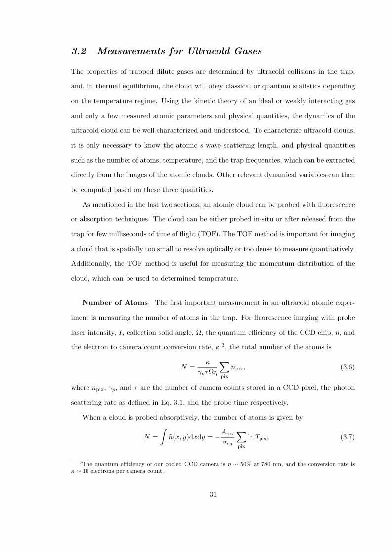
Number of Atoms The first important measurement in an ultracold atomic exper-

iment is measuring the number of atoms in the trap. For fluorescence imaging with probe

laser intensity, I, collection solid angle, Ω, the quantum efficiency of the CCD chip, η, and

the electron to camera count conversion rate, κ 3, the total number of the atoms is

N =κ

γpτΩη

∑

pix

npix, (3.6)

where npix, γp, and τ are the number of camera counts stored in a CCD pixel, the photon

scattering rate as defined in Eq. 3.1, and the probe time respectively.

When a cloud is probed absorptively, the number of atoms is given by

N =∫

n(x, y)dxdy = −Apix

σeg

∑

pix

ln Tpix, (3.7)

3The quantum efficiency of our cooled CCD camera is η ∼ 50% at 780 nm, and the conversion rate isκ ∼ 10 electrons per camera count.

31

where Apix is the area of each pixel, σeg is the absorption cross section of the cycling

transition, and Tpix is the transmission profile defined in the last section.

Temperature The temperature of the gas can be determined by measuring the mo-

mentum distribution of the cloud. When a thermal gas is released from the trap, the

momentum distribution of the atoms will be converted to a spatial density distribution.

For a gas far from the quantum degenerate regime, the momentum distribution will have

an isotropic gaussian form due to the equipartition theorem [76]. For an expanded cloud

that is much larger than the initial trap size, the measured cloud will provide an accurate

determination of the momentum distribution. Then the temperature can be extracted from

the width of this Gaussian distribution. Fig. 3.1.a illustrates the time-of-flight images of

thermal clouds.

By collapsing a cloud image to a 1D density profile as shown in Fig. 3.1.b, the Gaussian

waist can be found as σ = FWHM/(2√

2 ln 2), where FWHM is the full width at half

maximum. With this measured Gaussian waist, the temperature can be readily found as

T =m

kB(σ

t)2. (3.8)

Here, m is the mass of a 87Rb atom, kB is the Boltzmann constant, and t is the free expansion

time of the cloud after it is released from the trap. If the initial size of the trapped cloud

is too large to be neglected, the cloud temperature can be determined by two images with

different drop times;

T =m

kB

(σ2

2 − σ21

t22 − t21

). (3.9)

Here, σ1,2 are the Gaussian waist at drop time t1,2. From Fig. 3.2, it is clear that Eq. 3.9 is

a better algorithm for computing the temperature. In addition, one can also measure the

cloud size for various drop times, and then fit the cloud expansion rate with a quadratic

equation: σ2 = σ20 + kBT

m t2. This way, one can not only find the temperature, T , but also

σ0, which is the cloud waist at t = 0.

Trap Frequencies Trap frequencies are measured using a parametric resonance tech-

nique [77]. The governing equation for parametric resonance for a parametrically driven

32

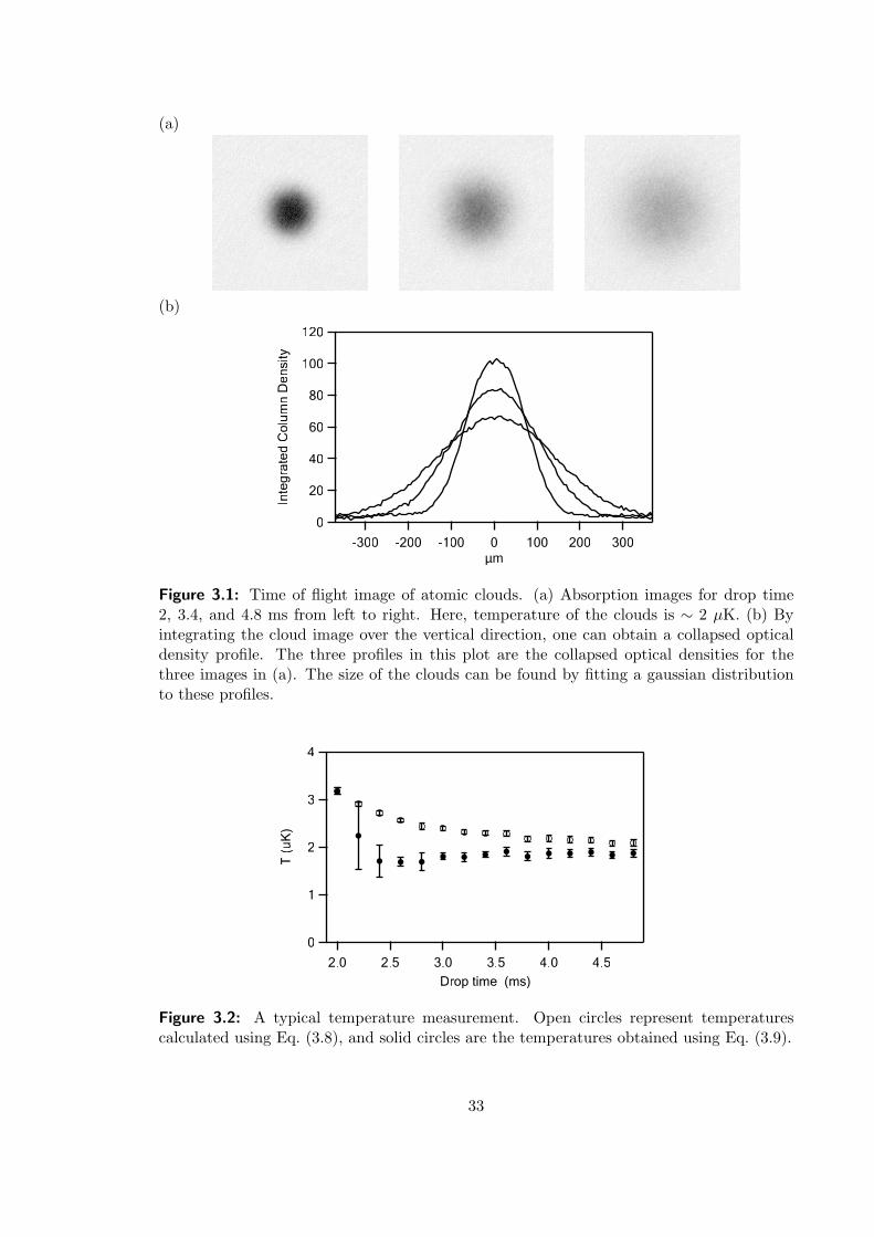
(a)

(b)

120

100

80

60

40

20

0

Inte

gra

ted

Co

lum

n D

en

sity

-300 -200 -100 0 100 200 300

µm

Figure 3.1: Time of flight image of atomic clouds. (a) Absorption images for drop time2, 3.4, and 4.8 ms from left to right. Here, temperature of the clouds is ∼ 2 µK. (b) Byintegrating the cloud image over the vertical direction, one can obtain a collapsed opticaldensity profile. The three profiles in this plot are the collapsed optical densities for thethree images in (a). The size of the clouds can be found by fitting a gaussian distributionto these profiles.

4

3

2

1

0

T (

uK

)

4.54.03.53.02.52.0

Drop time (ms)

Figure 3.2: A typical temperature measurement. Open circles represent temperaturescalculated using Eq. (3.8), and solid circles are the temperatures obtained using Eq. (3.9).

33

120

100

80

60

40

20

0

N (x10

3)

50004000300020001000Frequency (Hz)

400

300

200

100

0

T (

µK)

Figure 3.3: Trap frequency measurement by parametric resonance. The cloud is weaklyheated at trap frequencies, and are severely heated at twice the trap frequencies. Here thesolid line is the temperature, and the dotted line is the number of atoms.

harmonic oscillator is

x = ω2(1 + ε sinΩt)x , (3.10)

where ω is the trap frequency, and ε and Ω are the modulation amplitude and frequency.

When the modulation frequency equals 2ω/n, where n is an integer, the energy of the

oscillator grows exponentially [78]. We can employ this idea to excite/heat the atoms in the

trap. The trap frequencies can be modulated by modulating the trap depth, since ω ∝ √U ,

and to modulate the trap depth, we simply modulate the CO2 laser power. When the cloud

is parametrically excited, especially at 2ω, atoms are strongly heated and boiled away. By

measuring the temperature and/or the number of atoms left in the trap vs. modulation

frequency, one can then determine the trap frequencies. Fig. 3.3 shows typical results of

trap frequency measurements. In this particular case, the CO2 power is ramped down after

trap loading to evaporatively cool the cloud to few µK, which is low but still above the

BEC critical temperature. Then the CO2 power is adiabatically ramped back up to 5 W to

compress the trap, and immediately amplitude modulated with 10% modulation for 0.5 s.

The cloud is then released to measure the temperature and the total number of atoms. As

shown in the plot, when the modulation frequency hits twice the trap frequency, the cloud

is severely heated.

34

Density of a Trapped Thermal Cloud We can determine the trapped cloud density

from the measured number of atoms, the temperature, and the mean trap frequency. We

begin by approximating the optical trap potential to a harmonic potential. The total

number, N , and the peak density of the cloud are related as

N =∫

n0 e−mωr2

2kBT d3r = n0(2πkBT

mω2)3/2, (3.11)

where T , m, and ω are the temperature, mass of 87Rb, and mean trap frequency, ω =

(ωxωyωz)1/3. Solving for the peak density, we find

n0 = N(mω2

2πkBT)3/2. (3.12)

Collision Rates Ultracold collisions play a major role in determining the properties

of the Bose-Einstein condensates. Elastic collisions in trapped gas are also essential for

establishing equilibrium and are necessary for evaporative cooling. Efficient evaporative

cooling requires that elastic collisions dominate inelastic or other non-evaporative trap loss

collisions such as three-body recombination or collisions between the trapped cloud and the

residual background gas. In general, higher elastic collision rates will allow faster and more

efficient evaporation.

In a thermal cloud, the mean thermal velocity is v =√

8kBTπm , and the average relative

velocity of two particles is vrel =√

2v. For low energy collisions, the collision cross section

is simply σsc = 2 × π (2a)2, where a is the s-wave scattering length, and the factor of 2

comes from the indistinguishability of two identical bosons. The two-body elastic collision

rate is given by

γel = n0 σsc vrel = N(8√

2a2m

πkB)ω3

T. (3.13)

While discussions on ultracold collisions in this thesis and in the majority of the com-

munity focus on two-body (elastic) collisions, three-body inelastic collisions become non-

negligible when the cloud density is > 1014 cm−3 and result in trap loss. The three-body

collision (loss) rate can be calculated as

γ3B = Γ3B

∫n3(~r)d3r. (3.14)

35

At temperatures much higher than the BEC critical temperature, the cloud density is given

by Eq. 3.11, and the three-body collision rate is

γ3B = Γnc3B

n20N√27

. (3.15)

For a condensate with a Thomas-Fermi wavefunction, which is given by Eq. 3.29 in the next

section, the three-body collision rate is found to be

γ3B = Γc3B

8n20N

21. (3.16)

Here, n0 is the peak cloud density, and the rate constants for 87Rb thermal clouds and

condensates are Γnc3B = 4.3(1.8)×10−29 cm6/s, and Γc

3B = 5.8(1.9)×10−30 cm6/s, respectively

[18]. It is noted that Γnc3B/Γc

3B ' 3! due to the higher order coherence in the condensate [18].

Phase Space Density The phase space density, Λ, characterizes the number of atoms

occupying a single quantum state, and the onset of quantum degeneracy requires Λ ∼1. This important quantity is defined as the particle density in the joint coordinate and

momentum space, and the peak phase space density for a trapped gas is given by

Λ0 ≡ n0λ3dB, (3.17)

where n0 is the peak spatial density, and λdB = h/√

2πmkBT is the thermal de Broglie

wavelength. When the temperature is much higher than the BEC critical temperature such

that Λ0 ¿ 1, the Bose distribution can be approximated by the Boltzmann distribution,

and Λ0 is related to the total number of atoms via the integral:

N =Λ0

h3

∫e−

mω2

2kBTr2

e−p2

2mkBT d3rd3p = Λ0

(kBT

~ω

)3

.

Therefore,

Λ0 = N

(~ωkBT

)3

. (3.18)

Although this expression is an approximation, it is very useful for estimating the efficiency

of evaporative cooling in real time, and it can be used as the figure of merit for tailoring

and optimizing the evaporation trajectory.

36

3.3 Image Analysis for Ultracold Clouds Near BEC Tran-sition Temperatures

When the temperature is very close to the critical temperature of quantum phase transition,

the properties of a cloud will deviate from that of a classical gas, and the treatments in the

last section based on Boltzmann statistics are insufficient. In this temperature regime, image

analysis based on Bose statistics is necessary. For clarity, the relevant physical quantities

will be derived from first principle, and the approach here follows closely to ref. [9].

The Bose distribution function is given by

n =1

e−(µ−H)/kBT − 1=

∞∑

j=1

(z e−H/kBT )j , (3.19)

where H is the system Hamiltonian, µ is the chemical potential, and z = eµ/kBT is the

fugacity 4. The Hamiltonian of an ideal gas confined in a harmonic trap is just that of

uncoupled harmonic oscillators,

H =3∑

i=1

(p2

i

2m+

mω2i r

2i

2), (3.20)

where ω1,2,3 are the trap frequencies of the trap.

Total Number of Atoms in Excited States Integrating the Bose distribution

function over all phase space yields the total number of atoms in the excited states (thermal

atoms):

Nth =1h3

∫d3rd3p

∞∑

j=1

(z e−H(~r,~p)/kBT )j (3.21a)

= (kBT

~ω)3g3(z), T ≥ Tc, (3.21b)

where ω is the mean trap frequency, and g3(z) is the Riemann Zeta function of fugacity z

5. When the temperature T is below the critical temperature Tc, Nth is less than the total

number of atoms in the trap, and the excess atoms are populated in the ground state of

4In Eq. 3.20 we have used the identity: 1x−1

=∞P

j=1

( 1x)j , x > 1.

5Riemann Zeta function gl(z) ≡∞P

j=1

zj

jl

37

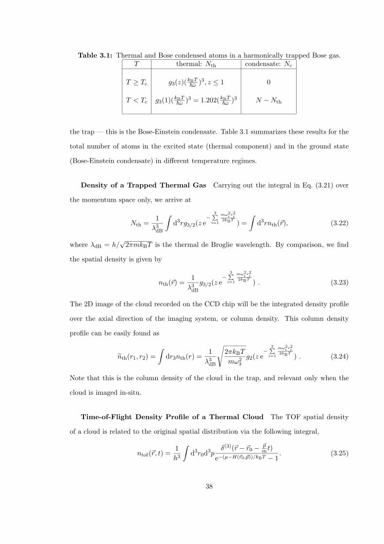
Table 3.1: Thermal and Bose condensed atoms in a harmonically trapped Bose gas.T thermal: Nth condensate: Nc

T ≥ Tc g3(z)(kBT~ω )3, z ≤ 1 0

T < Tc g3(1)(kBT~ω )3 = 1.202(kBT

~ω )3 N −Nth

the trap — this is the Bose-Einstein condensate. Table 3.1 summarizes these results for the

total number of atoms in the excited state (thermal component) and in the ground state

(Bose-Einstein condensate) in different temperature regimes.

Density of a Trapped Thermal Gas Carrying out the integral in Eq. (3.21) over

the momentum space only, we arrive at

Nth =1

λ3dB

∫d3rg3/2(z e

−3P

i=1

mω2i r2

i2kBT ) =

∫d3rnth(~r), (3.22)

where λdB = h/√

2πmkBT is the thermal de Broglie wavelength. By comparison, we find

the spatial density is given by

nth(~r) =1

λ3dB

g3/2(z e−

3Pi=1

mω2i r2

i2kBT ) . (3.23)

The 2D image of the cloud recorded on the CCD chip will be the integrated density profile

over the axial direction of the imaging system, or column density. This column density

profile can be easily found as

nth(r1, r2) =∫

dr3nth(r) =1

λ3dB

√2πkBT

mω23

g2(z e−

2Pi=1

mω2i r2

i2kBT ) . (3.24)

Note that this is the column density of the cloud in the trap, and relevant only when the

cloud is imaged in-situ.

Time-of-Flight Density Profile of a Thermal Cloud The TOF spatial density

of a cloud is related to the original spatial distribution via the following integral,

ntof(~r, t) =1h3

∫d3r0d3p

δ(3)(~r − ~r0 − ~pm t)

e−(µ−H(~r0,~p))/kBT − 1. (3.25)

38

Assuming that the expansion time t >> ω−11 , ω−1

2 , ω−13 , the TOF density is given by

ntof(~r, t) =1

λ3dB

1(ωt)3

g3/2(z e−m

2kBT

r21+r2

2+r23

t2 ) . (3.26)

Integrating over the direction of optical axis of the imaging system, we obtain the column

density,

ntof(r1, r2, t) = A g2(z e−r21+r2

22σ2 ), (3.27)

where A = 1λ3dB

1(ωt)3

√2πkBT

m t2, and σ2 = kBTm t2.

Density and Radii of a Trapped BEC At zero temperature, the dynamics of a

trapped BEC are described by the Gross-Pitaevskii (or nonlinear Schrodinger) equation

[24]. Within the Thomas-Fermi (T-F) approximation [20, 79], in which the kinetic energy

or the quantum pressure is neglected, the density in the trap is given by

nTF(~r) = max(

µ− U(~r)g

, 0)

. (3.28)

Here U(~r) is the trap potential, µ is the chemical potential, and g = 4π~2a/m is the two-

body interaction strength, where a is the s-wave scattering length. It is readily found that

the density of the condensate in a harmonic trap, n ∝ |ψ(r)|2, has the form of an inverted

parabola [20, 79],

nTF(~r) =15N

8πΠiRi,cmax(1−

3∑

i=1

r2i

R2i,c

, 0), (3.29)

and the column density is

nTF(~r) = nc(0)max(1−2∑

i=1

r2i

R2i,c

, 0)3/2, (3.30)

where nc(0) is the peak column density, and Ri,c are the radii of the T-F order parameter.

Here, Ri,c are given by

Ri,c =

√2µ

mω2i

. (3.31)

The chemical potential is required to compute the T-F radii Ri,c, and it can be calculated

using Eq. 3.28 with a harmonic trap potential and the normalization condition for the order

parameter,∫

n(~r)d3r = N (see Appendix F). The chemical potential is calculated as

µ =

(15~2m1/2

25/2Nω3a

)2/5

, (3.32)

39

where N is the number of atoms, ω is the mean trap frequency, and a is the s-wave scattering

length.

Time-of-Flight Density of a BEC The time-of-flight (TOF) images were first used

to distinguish Bose-Einstein condensates from thermal clouds [1, 3], and the characteristic

anisotropy of the expansion of condenstes released from non-spherical traps remains the

standard signature of a condensate. For non-spherical trapping potentials, the direction

with tighter confinement will lead to higher momentum and higher expansion rate along

that direction. The TOF density profile is a simple rescaling of the in-situ condensate

spatial density profile given by Eq. 3.29, and at any given infinitesimal expansion time, the

TOF radii expand along a trajectory [80]

Ri(t) = λi(t)Ri(0), i = 1, 2, 3 , (3.33)

where λi(t) satisfy

λi(t) =ω2

i (0)λiλ1λ2λ3

, i = 1, 2, 3. (3.34)

Specifically, for a cigar shape condensate (ω1 = ω2 = ω⊥ À ωz), the radii will grow according

to [80]

Rc,⊥(τ) = Rc,⊥(0)√

1 + τ2, (3.35a)

Zc(τ) ' Zc(0)[1 + ε2(τ arctan τ − ln√

1 + τ2)], (3.35b)

where τ = ω⊥t is the scaled expansion time, and ε = ωz/ω⊥ ¿ 1 is the inverse of the aspect

ratio of the trap. These equations can be used to determine the density of a BEC directly

from time of flight images.

2D Image Fit for Atomic Clouds To extract the temperature, number of atoms,

and other quantities from the images, we fit the images with 2D functions. For T À Tc we

simply fit a 2D Gaussian to the cloud image. For T & Tc, it is found that 2D Gaussian

fit always underestimates the temperature. We therefore fit a 2D Gaussian to the wings

of the cloud image, and then use the fit results as initial conditions for fitting the Bose

40

function given in Eq. (3.27) to the image. For T < Tc the cloud has both a thermal gas and

condensate component, so we fit to the sum of Eq. (3.27) and Eq. (3.30). Therefore,

ntof,th(~r) = A e−r21+r2

22σ2 , T À Tc (3.36a)

ntof,tot(~r) = Ag2(z e−r21+r2

22σ2 ), T & Tc (3.36b)

ntof,tot(~r) = Ag2(e− r2

1+r22

2σ2 ) + B max(1−2∑

i=1

r2i

R2i

, 0)3/2, T ≤ Tc (3.36c)

where A, z, σ, B, and Ri’s are free fitting parameters.

The image fitting is very useful for extracting important physical quantities. However,

it is noted that the fitting routines in certain conditions do not converge to a single valued

result. Firstly, the fit to the Bose function when T > Tc does not always result in unique

values of A, z, and σ. Secondly, it is known that the presence of a condensate causes

depletion of thermal atoms at trap center due to atomic interactions [81]. Since the ideal

gas ansatz given above does not account for the repulsive interactions between condensate

and thermal gas due to the positive scattering length of 87Rb, it will tend to overestimate

the number of thermal atoms and underestimate the number of condensed atoms. Thirdly,

a bimodial fitting is not robust when one component is significantly smaller than the other.

This happens at the onset of the Bose-Einstein condensation, where the BEC component

is much smaller than the thermal gas, and for T ¿ Tc when the cloud is almost a pure

condensate. Nonetheless, the fitting models provide a reasonable approximation to the real

physical system. For illustration purposes, a 2D image fit at temperature at 2Tc is shown

in Fig. 3.4, and a typical bimodal fit to a partially condensed cloud is displayed in Fig. 3.5.

In the studies of large spinor condensates, spin domains are observed to form in different

spin components. While the total condensate wavefunction fits well with the Thomas-Fermi

form, the wavefunction for each spin component can not be described by a simple Thomas-

Fermi form due to domain formation. So, for image fitting to a spinor condensate, we only

fit the Bose function with fugacity z = 1 to the wings of the thermal component, or

ntof(r1, r2, t) = Ag2(e− r2

1+r22

2σ2 ), (3.37)

This is done by masking off the central region where the condensate resides. Fig. 3.6

41

raw Gaussian resid EnBose resid

1.5

1.0

0.5

0.0

Opt

ical

den

sity

2001000Pixel

Gaussianx-slice

1.5

1.0

0.5

0.0

2001000

Gaussiany-slice

Pixel Size (m) = 2.99e-06

Img Size (pix) = 240x240

Drop Time (s) = 0.009

Trap Freq (Hz) = 86.993

T (nK) = 692

PSD = 0.13

Therm N (k) = 605

T (nK) = 745

PSD = 0.26

Therm N (k) = 580

ChiSqr Gaussian = 42.928

ChiSqr EnBose = 54.2641.5

1.0

0.5

0.0

2001000

Bosey-slice

1.5

1.0

0.5

0.0

2001000

Bosex-slice

Density (1/cm3) = 1.2e+13

Density (1/cm3) = 1.0e+13

T/Tc = 2.1

T/Tc = 2.3

Figure 3.4: 2D image fits for a thermal cloud. The images shown here are the fitting resultsof the Gaussian fit and Bose fit for the mF = −1 component in a spinor condensate. Whenthe temperature is close to the critical temperature, the Gaussian fit always underestimatesthe temperature. In addition, the Gaussian ansatz does not fit well to the central part ofthe cloud. Therefore, this ansatz only fits the tails of the thermal cloud. The fit resultsare then used as initial conditions for fitting with a Bose distribution. Top images (left toright) are raw image, image with the Gaussian fit subtracted, and image with the Bose fitsubtracted, respectively.

42

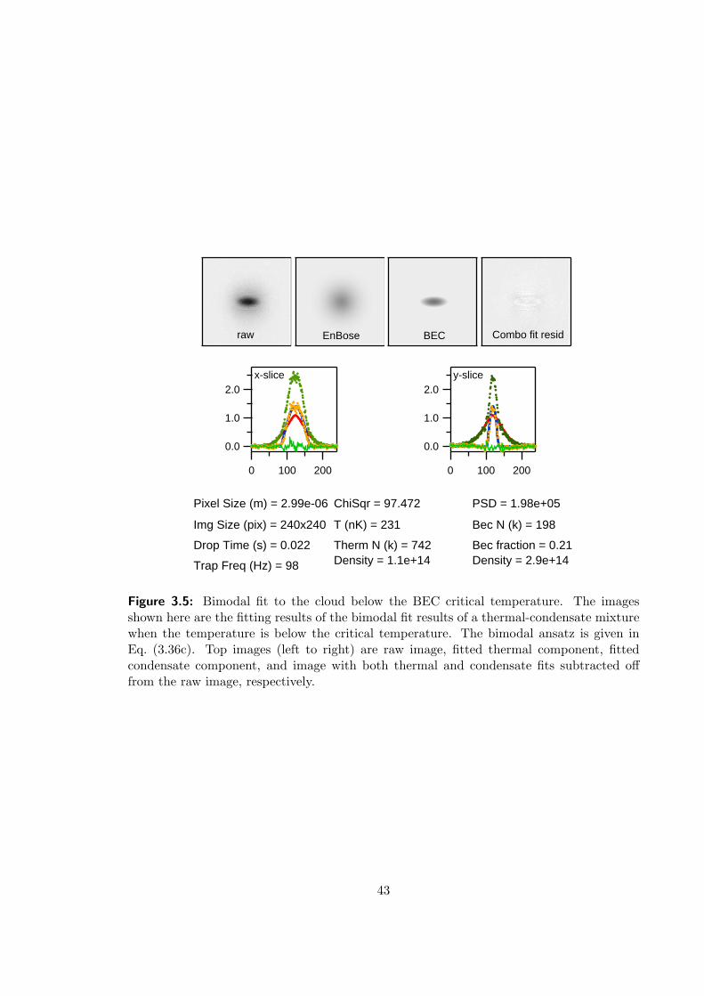
2.0

1.0

0.0

2001000

y-slice

raw

2.0

1.0

0.0

2001000

x-slice

Pixel Size (m) = 2.99e-06

Drop Time (s) = 0.022

Trap Freq (Hz) = 98

T (nK) = 231

Therm N (k) = 742

Bec N (k) = 198

Bec fraction = 0.21

Combo fit resid

Img Size (pix) = 240x240

ChiSqr = 97.472

Density = 1.1e+14

PSD = 1.98e+05

Density = 2.9e+14

EnBose BEC

Figure 3.5: Bimodal fit to the cloud below the BEC critical temperature. The imagesshown here are the fitting results of the bimodal fit results of a thermal-condensate mixturewhen the temperature is below the critical temperature. The bimodal ansatz is given inEq. (3.36c). Top images (left to right) are raw image, fitted thermal component, fittedcondensate component, and image with both thermal and condensate fits subtracted offfrom the raw image, respectively.

43

raw EnBose residEnBose fit

1.5

1.0

0.5

0.0

2000

x-slice1.5

1.0

0.5

0.0

2000

y-slice

Pixel Size (m) = 2.99e-06

Img Size (pix) = 240x240

Drop Time (s) = 0.012

Trap Freq (Hz) = 69.874

T (nK) = 570

PSD = 7.5e+5

Therm N (k) = 219 Becfraction = 0.25

BEC

Mask

Density (cm-3

)= 2.9e+12

Bec N (k) = 75

Density (cm-3

) = 1.3e+14

ChiSqr = 37.141

Figure 3.6: Bose fit to wings of the thermal cloud with fugacity z = 1. The images shownhere are the fitting results of the |F = 1,mF = 0〉 spin component. To fit to the wings ofthe thermal cloud only, we apply a ellipse mask to exclude fitting to the central area wherethe condensate resides. This fit is useful when the condensate is not of the simple Thomas-Fermi form, which often happens when spin domains developed in a large spinor condensatesuch as in this particular case. Top images (left to right) are the mask, raw image, thermalcomponent, and image with thermal component subtracted off the raw image (condensatecomponent), respectively.

illustrates the results of a typical fit with the Bose function. Again, the fit results generally

depends on the mask shape and size, and the results may vary up to 50% due to change of

applying masks.

Phase Space Density (PSD) When the temperature T ≥ Tc, the peak PSD is given

by

Λ0 = λ3dBn0 = g3/2(z), z ≤ 1. (3.38)

Here, Tc is the critical temperature, and z is the fugacity. In a case where T >> Tc, z is much

less than 1 and the PSD is approximated as Λ0 ' z. To compute the PSD, a knowledge of

the fugacity or chemical potential is necessary. However, they are often difficult to measure.

Recall that when T >> Tc a Bose distribution function is approximated by a Boltzmann

44

Table 3.2: Phase space density in different temperature regime. Here z = eµ/kBT is thefugacity, and µ is the chemical potential.

T Λ0 Λ′ (Approx.)T ≥ Tc g3/2(z), z ≤ 1 N( ~ωkBT )3 = g3(z)

z

T = Tc g3/2(1) = 2.612

T < Tc Nc

distribution, then the PSD can be conveniently estimated using Eq. 3.18.

When T < Tc, the total number of atoms is greater than the available occupation

number in the excited states, and the excess atoms will Bose condense in the ground state.

This results in a macroscopic number of atoms sharing a single quantum state, i.e., the

ground state. Then the peak PSD is simply Λ0 = Nc, where Nc is the number of atoms in

the condensate.

Table 3.2 lists the phase space density and its approximation in different temperature

regimes, and the numerical error due to the approximation is given in Fig. 3.7. When the

temperature T & Tc, the approximation error can be as large as 60%. Nevertheless, the

approximation given by Eq. 3.18 is easy to apply and useful for characterizing evaporative

cooling trajectories which will be seen in the next chapter.

45

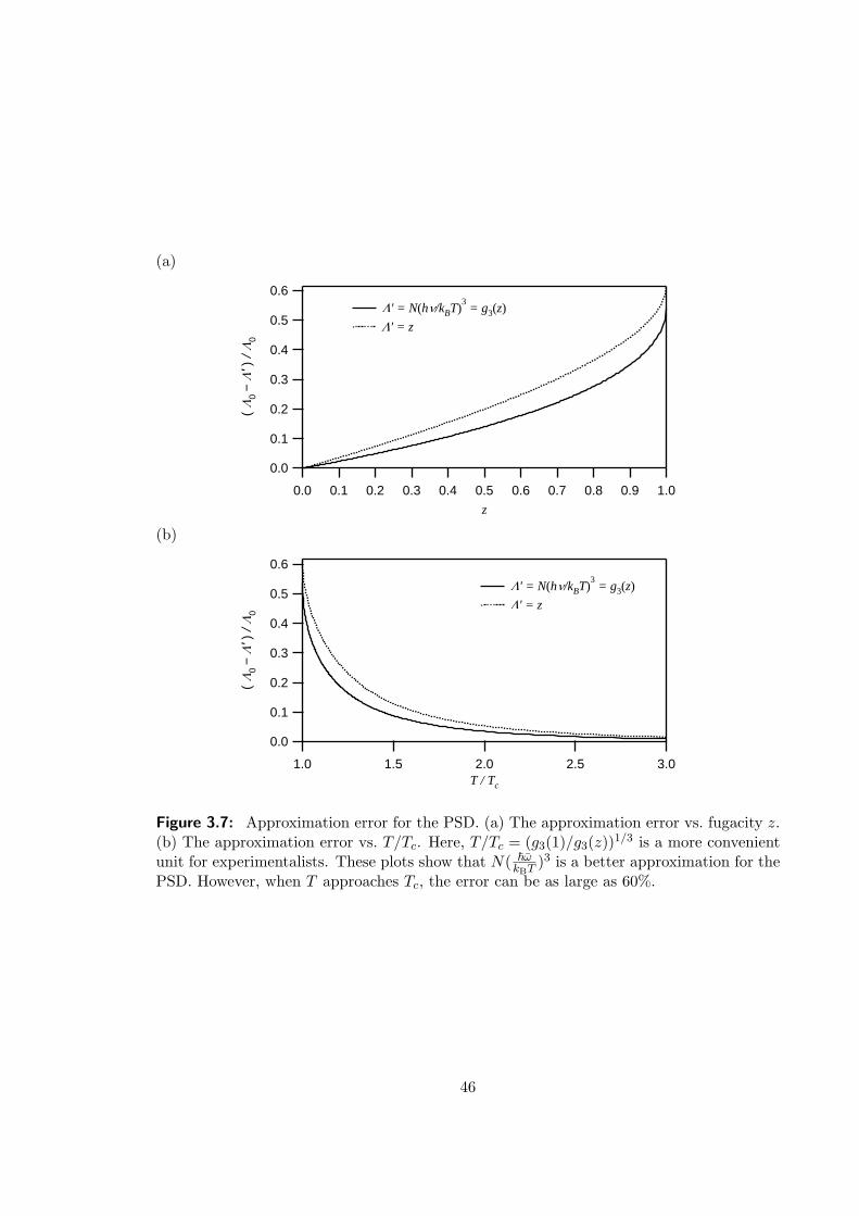
(a)

0.6

0.5

0.4

0.3

0.2

0.1

0.0

( L

0 − L

' ) / L

0

1.00.90.80.70.60.50.40.30.20.10.0

z

L' = N(hn/kBT)3 = g3(z)

L' = z

(b)

0.6

0.5

0.4

0.3

0.2

0.1

0.0

( L

0 − L

' ) /

L0

3.02.52.01.51.0T / Tc

L' = N(hn/kBT)3 = g3(z)

L' = z

Figure 3.7: Approximation error for the PSD. (a) The approximation error vs. fugacity z.(b) The approximation error vs. T/Tc. Here, T/Tc = (g3(1)/g3(z))1/3 is a more convenientunit for experimentalists. These plots show that N( ~ωkBT )3 is a better approximation for thePSD. However, when T approaches Tc, the error can be as large as 60%.

46

CHAPTER IV

ALL-OPTICAL BEC EXPERIMENTS

Given the tremendous impact of BEC research in the last 11 years and the continued growth

of the field, it is important to explore different methods for reaching BEC, particularly

methods that offer new capabilities, simplicity, or speed. Our group demonstrated such a

method by creating a Bose condensate of 87Rb atoms directly in a crossed-beam optical

dipole force trap of tightly focused CO2 laser beams [34]. In the broader scope of research

with ultracold degenerate gases, our system stood out for several reasons. First, all-optical

BEC provided the first new path to achieving BEC since the first pioneering demonstrations

[1, 3, 2], and it was surprisingly simple and an order of magnitude faster than standard BEC

experiments. Secondly, optical trapping potentials can be essentially spin-independent and

hence offer unique capabilities for trapping atoms and molecules not amenable to magnetic

trapping. In particular, all-optical BEC experiments are ideally suited for studying the

dynamics of condensates with internal spin, or spinor condensates. Since the realization

of our first all-optical BEC in 87Rb [34, 82, 83], several other atoms, Cs [84], Yb [36], Na

[85], and (fermionic) 6Li [86] have been condensed in all-optical traps as well. Finally, a rich

variety of spatial confinement geometries can be easily engineered in optical traps, including

large period one- to three-dimensional lattices in which individual sites can be resolved and

addressed [87]. This technical advantage allows optical traps to find applications in testing

condensed matter theories [14, 88] and in quantum information science [89, 90, 91, 92]. In

this chapter, we give an overview of our all-optical BEC techniques.

4.1 Review of First All-Optical BEC

All-optical methods of reaching the BEC phase transition have been pursued since the early

days of laser cooling [93, 94]. Evaporative cooling in optical traps was first demonstrated in

1994, where, starting with only 5000 atoms, a phase space density increase of a factor of 30

47

was realized [70]. Whereas the first demonstrations of evaporative cooling of alkali atoms

in magnetic traps lead quickly to the observation of BEC, the progress in optical traps

was slower. A principle challenge faced by all-optical traps was that the small trap volume

provided by the focused lasers (typically much less than 1 mm3) limits the number of atoms

that can be loaded in the trap. Also, lowering the trap depth to force evaporation also lowers

the trap oscillation frequency and the rethermalization rate. Hence the evaporation rate

can slow down prohibitively. Finally, optical traps have historically suffered from excessive

heating rates either due to intrinsic spontaneous scattering of photons from the trapping

beams or the technical noise of the trapping laser [95, 96]. Best previous efforts on optical

trapping beyond the limits set by Doppler cooling yielded atomic phase space densities a

factor of 3 away from the BEC transition [73, 97].

Despite the technical challenges, our group successfully realized the first all-optical BEC

experiment in 2001 [34]. In this impressive experiment Murray Barrett et al. employed a

CO2 laser dipole force trap [98] in a cross trap geometry. Each beam had a maximum power

of 12 W, and the beams were focused to a minimum waist ∼50 µm. Initially 2× 106 atoms

were loaded at a temperature of 70 µK and densities > 1014 atoms/cm3. Forced evaporative

cooling of the atomic sample was achieved by lowering the trap beam powers 50-fold over 2

s. The BEC transition occurred at temperature of ∼ 300 nK and beam powers of 300 mW.

At the lowest final temperature, mostly pure condensate which contained 30,000 atoms was

created [34, 62].

The initial success in achieving BEC in an optical trap hinged on the very high spatial

and phase space densities achieved during the loading process. The initial spatial density

loaded into the cross dipole trap exceed 1014 atoms/cm3, which is 3 orders of magnitude

higher than that of the loading MOT. Given the well-known density limitations in laser

cooling due to reabsorption of scattered radiation and photo-associative losses induced by

the cooling fields, it is surprising that such high densities could be achieved in an optical

trap using only standard sub-Doppler cooling techniques. Although loading of optical dipole

traps has been the subject of several experimental [77, 99] and theoretical [100] studies, none

of these apply specifically to our configuration.

48

The next section will be devoted to the studies on CO2 laser trap loading dynamics.

We note that the these studies were begun by Murray Barrett while finishing up his PhD

thesis. Since the impressive results carried out by Murray are yet unpublished, and a better

knowledge of loading dynamics is essential for developing new trap geometries, we will

summarize them in the next section. The understanding of trap loading also led Murray

to directly create condensates in 1-D lattice. We will also summarize the 1-D lattice BEC

experiment later in this chapter. Finally, we note that while the experimental techniques

for the 1-D lattice were developed by Murray, most of the data presented here were taken

at a later date by myself.

4.2 Trap Loading Studies

Our BEC experiments employ CO2 laser optical traps loaded from a standard 87Rb vapor

cell MOT [62]. The experiment begins with loading the MOT for 10 s directly from the

thermal vapor during which we collect up to 5 × 108 atoms. After loading the MOT, the

cooling configuration is changed to achieve sub-Doppler cooling in order to maximize the

transfer of atoms to the optical trap. The repump intensity is first lowered to 15 µW/cm2

for 20 ms, and then the MOT trap beams are detuned to the red of the trapping transition

by 140 MHz for 40 ms. At this point the MOT beams are extinguished, and the current in

the MOT coils is turned off. In order to optically pump the atoms into the F = 1 hyperfine

states, the repump light is shuttered off 1 ms before the trap beams are extinguished; the

efficiency of the optical pumping to the F = 1 state are measured to be > 95%. The

CO2 laser beams are left on at full power throughout the MOT loading and dipole trap

loading process. This sub-Doppler cooling scheme is a variation of the temporal dark MOT

technique [66], and the timing scheme is illustrated in Fig. 4.1. This cooling step is crucial

for efficient loading into the optical trap.

The results of loading the single focused beam trap, the 1-D lattice trap, as well as the

cross trap are summarized in the first three columns of Table 4.1 [62]. The 1-D lattice is

obtained by retro-reflecting the laser beam, and it produces an array of microtraps separated

by half the wavelength (5.3 µm) [77]. While each of these traps provide much higher spatial

49

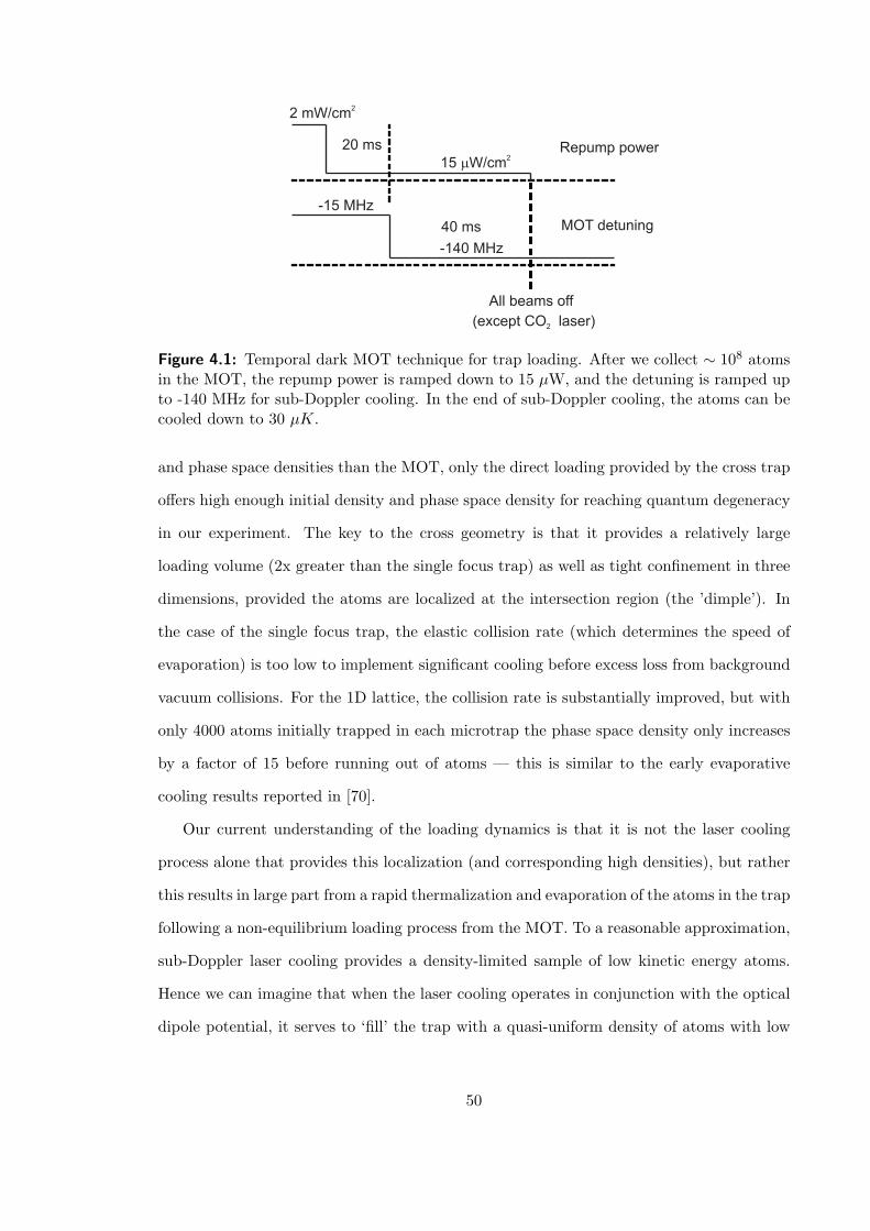
Repump power

MOT detuning

-140 MHz

-15 MHz

15 W/cmm2

20 ms

40 ms

All beams off

(except CO laser)2

2 mW/cm2

Figure 4.1: Temporal dark MOT technique for trap loading. After we collect ∼ 108 atomsin the MOT, the repump power is ramped down to 15 µW, and the detuning is ramped upto -140 MHz for sub-Doppler cooling. In the end of sub-Doppler cooling, the atoms can becooled down to 30 µK.

and phase space densities than the MOT, only the direct loading provided by the cross trap

offers high enough initial density and phase space density for reaching quantum degeneracy

in our experiment. The key to the cross geometry is that it provides a relatively large

loading volume (2x greater than the single focus trap) as well as tight confinement in three

dimensions, provided the atoms are localized at the intersection region (the ’dimple’). In

the case of the single focus trap, the elastic collision rate (which determines the speed of

evaporation) is too low to implement significant cooling before excess loss from background

vacuum collisions. For the 1D lattice, the collision rate is substantially improved, but with

only 4000 atoms initially trapped in each microtrap the phase space density only increases

by a factor of 15 before running out of atoms — this is similar to the early evaporative

cooling results reported in [70].

Our current understanding of the loading dynamics is that it is not the laser cooling

process alone that provides this localization (and corresponding high densities), but rather

this results in large part from a rapid thermalization and evaporation of the atoms in the trap

following a non-equilibrium loading process from the MOT. To a reasonable approximation,

sub-Doppler laser cooling provides a density-limited sample of low kinetic energy atoms.

Hence we can imagine that when the laser cooling operates in conjunction with the optical

dipole potential, it serves to ‘fill’ the trap with a quasi-uniform density of atoms with low

50

Table

4.1

:C

ompa

riso

non

Opt

ical

Tra

pLoa

ding

.N

ote

that

exce

ptth

enu

mbe

rof

atom

s,ot

her

quan

titi

esar

em

easu

rem

ent

atth

erm

aleq

uilib

rium

.

Sing

leB

eam

1-D

Lat

tice

Cro

ss1-

DLat

tice

Sing

leB

eam

(Dir

ect

load

ing)

(Tra

nsfe

rred

)(L

arge

volu

me)

Tra

pped

atom

s1×

106

1×

106

2×

106

1×

106

30×

106

(250

mic

rotr

aps)

(1-

4m

icro

trap

s)Tem

pera

ture

(µK

)20

3575

1012

0Pot

enti

alde

pth

(µK

)35

023

070

012

080

0Tra

pfr

eque

ncy

(Hz)

550

3000

1600

2100

500

Den

sity

(cm−3

)>

1012

1013

>10

14

>10

14

>10

13

Pha

sesp

ace

dens

ity

>0.

0001

0.00

030.

001

-0.

005

>0.

010.

0001

Col

lisio

nra

te(s−1

)20

080

010

,000

10,0

0010

,000

(tra

pco

mpr

essi

on)

Eva

pora

tion

Tim

e(s

)2

22

Bos

eco

nden

sed

atom

s30

,000

15,0

00-

30,0

0030

0,00

0

51

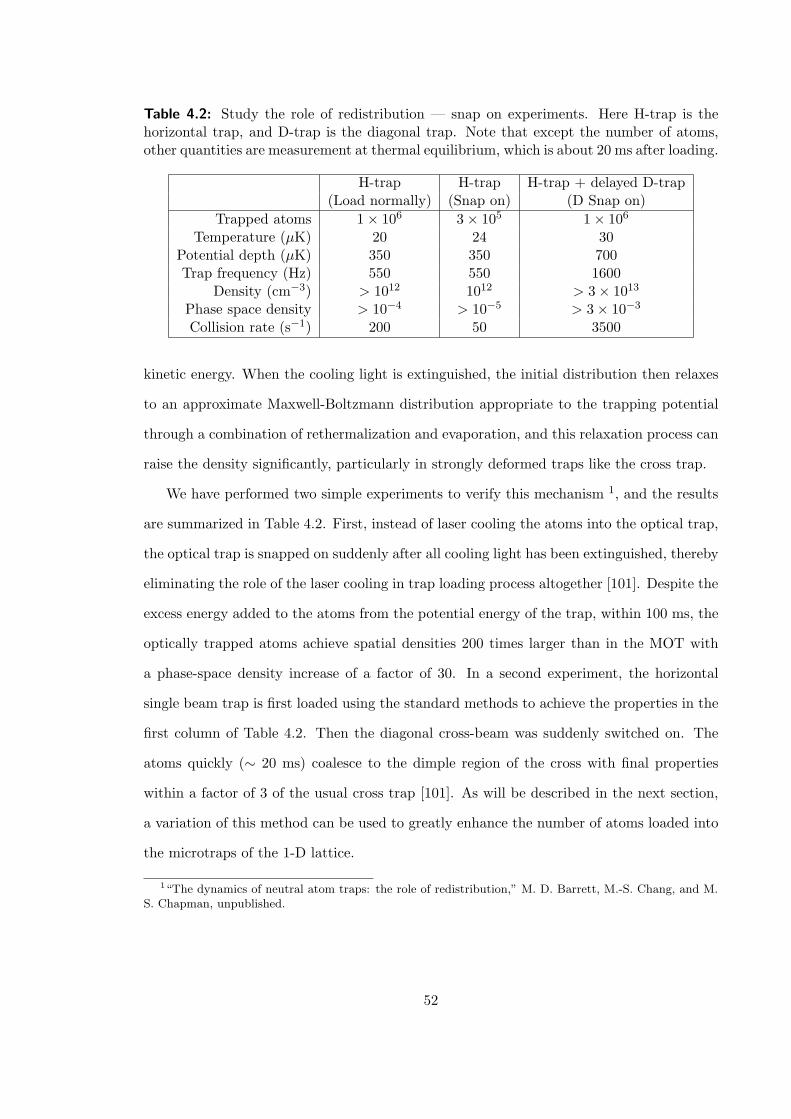
Table 4.2: Study the role of redistribution — snap on experiments. Here H-trap is thehorizontal trap, and D-trap is the diagonal trap. Note that except the number of atoms,other quantities are measurement at thermal equilibrium, which is about 20 ms after loading.

H-trap H-trap H-trap + delayed D-trap(Load normally) (Snap on) (D Snap on)

Trapped atoms 1× 106 3× 105 1× 106

Temperature (µK) 20 24 30Potential depth (µK) 350 350 700Trap frequency (Hz) 550 550 1600

Density (cm−3) > 1012 1012 > 3× 1013

Phase space density > 10−4 > 10−5 > 3× 10−3

Collision rate (s−1) 200 50 3500

kinetic energy. When the cooling light is extinguished, the initial distribution then relaxes

to an approximate Maxwell-Boltzmann distribution appropriate to the trapping potential

through a combination of rethermalization and evaporation, and this relaxation process can

raise the density significantly, particularly in strongly deformed traps like the cross trap.

We have performed two simple experiments to verify this mechanism 1, and the results

are summarized in Table 4.2. First, instead of laser cooling the atoms into the optical trap,

the optical trap is snapped on suddenly after all cooling light has been extinguished, thereby

eliminating the role of the laser cooling in trap loading process altogether [101]. Despite the

excess energy added to the atoms from the potential energy of the trap, within 100 ms, the

optically trapped atoms achieve spatial densities 200 times larger than in the MOT with

a phase-space density increase of a factor of 30. In a second experiment, the horizontal

single beam trap is first loaded using the standard methods to achieve the properties in the

first column of Table 4.2. Then the diagonal cross-beam was suddenly switched on. The

atoms quickly (∼ 20 ms) coalesce to the dimple region of the cross with final properties

within a factor of 3 of the usual cross trap [101]. As will be described in the next section,

a variation of this method can be used to greatly enhance the number of atoms loaded into

the microtraps of the 1-D lattice.

1“The dynamics of neutral atom traps: the role of redistribution,” M. D. Barrett, M.-S. Chang, and M.S. Chapman, unpublished.

52

a. b. c.

Figure 4.2: Loading atoms into only a few sites in an optical lattice. To transfer atoms froma single-focus trap to a 1-D optical lattice, the lattice is adiabatically turned on while thesingle-focus trap is adiabatically turned off. The transfer takes 50 ms, and we can transfernearly 100% of the atoms into only a few lattice sites.

Figure 4.3: Bose-Einstein Condensation in the 1-D lattice. Temperature is lowered acrossthe quantum Phase transition criticality (left to right).

4.3 Bose Condensation in 1D Lattice

Condensates in large period optical lattices have found several important applications due

to the potential of engineering controlled coupling between arrays of condensates. A 1-D

lattice was used in the first demonstration of Josephson tunneling between lattice wells [12],

the generation of number squeezed states [102], demonstration of dynamical tunneling [103],

and in transport measurements [104]. In a series of recent experiments with a 3-D lattice,

the Munich group has demonstrated a Mott insulator transition [14], and revivals of the

condensate wavefunction [105]. In all of these experiments, a sub-micron wavelength optical

lattice is employed, and hence the individual lattice sites are not observed. Instead, the

coupling between lattice sites is observed as an interference pattern between many phase

coherent condensates. The CO2 laser trap provides a lattice in a much different regime, with

a lattice spacing sufficiently large (5.3 µm) to optically resolve the individual microtraps

[87]. As we discuss below, it is even possible to isolate only 2 microtraps in the lattice to

realize a double well potential.

Our new understanding of the loading process has allowed us to increase the number of

53

atoms trapped in a lattice site by over a factor of 200, and with this, we have succeeded in

creating condensates directly in the lattice trap. To increase the number of atoms loaded in

the microtraps, we have implemented a loading scheme as shown in Fig. 4.2. A travelling

beam loads ∼ 106 atoms from the MOT and serves to ‘funnel’ a large number of atoms

into only a few microtraps when the crossed standing wave trap is turned on later. From

these initial conditions, evaporation proceeds readily as with the cross trap, and the BEC

transition occurs at a critical temperature, Tc = 800 nK with 110,000 atoms and trap

oscillation frequencies of (f1, f2, f3) = (100, 140, 3200) Hz. The loading parameters are

listed in the fourth column of Table 4.1, and images of evaporation in the lattice through

BEC phase transition is shown in Fig. 4.3.

4.3.1 Measurement and Control of The Lattice Sites Occupied

A unique feature of CO2 lattice is the large, (5.3 µm) spacing of the lattice sites. Our current

imaging system lacks sufficient resolution to image the individual microtraps. While this

will be upgraded in the future, in the meantime we have developed a technique to measure

the site occupancy in the standing wave traps by converting the spatial separation to a

separation in momentum space during time-of-flight imaging. This is done by superposing

a larger-scale optical harmonic potential along the direction of the standing wave, and

releasing the microtraps into this potential for a short duration before final release of the

atoms. Each microtrap is initially located at a different elevation of the added potential and

is subsequently accelerated towards the bottom of the potential at different rates. When the

added potential is also turned off, the microtrapped atoms will separate in space according

to their final velocity. The schematic and the time-of-flight (TOF) absorptive images of the

atomic clouds are illustrated in Fig. 4.4. With this diagnostic tool, we can have reasonably

precise control over the occupation of the microtraps by varying the cloud size in the single

focus beam and by changing the lattice site position upon the time of transfer to the lattice.

In Fig. 4.5 we demonstrate loading into one to three lattice sites. In the future, being able

to control loading in different sites will be a convenient experimental technique for studying

the dynamics and interplay of these microtrap condensate arrays.

54

(a)

(b)

t=0 trap off at t’’

image after 3ms

expansion

(c)

t’ = 0 0.1 0.2 0.3 0.4

0.5 0.6 0.7 0.8 0.9 (ms)

Figure 4.4: Measuring the lattice sites occupation. (a) In order to measure the numberof sites that are populated, we transfer the atoms back to the single-focus trap, and allowthe clouds to slosh inside a larger potential provided by this trap. With this technique, wecan convert the position dependent potential to the kinetic energy of the clouds. (b) Thetrap is turned off after various amount of slashing time, and each individual thermal cloudscan be optical resolved after 3 ms of TOF. (c) Absorptive images of actual measurements.The single-focus trap is oriented 45 with respect to the imaging axis, therefore, we canobserve 2-D harmonic motions when the two traps are not perfectly crossed. Meanwhile,this technique also allows us to visually measure the radial trap frequency. In this particularcase, the radial trap frequency is measured to be 1.4 kHz.

55

Figure 4.5: Image of the distinct microtraps following ’magnification’ provide by additionalharmonic confinement. Images show population of 1, 2 and 3 lattice sites (from left to right).

4.3.2 Matter Wave Interference

One of the hallmarks of BEC is the macroscopic quantum coherence of the gas. In a

well-known experiment performed by the MIT group [10], this coherence was observed as

matter-wave interference by releasing two condensates trapped in an elongated magnetic

trap separated by an optical dipole barrier. We have been able to observe interference fringes

in time of flight images of our released condensates as shown in Fig. 4.6. The three cases

in this figure corresponds to the three cases of site occupation in Fig. 4.5. The fringes for

two and three condensates are clearly seen, while for one condensate there is no discernible

fringes. The fringe contrast for the cases of two and three condensates are not very high.

It is typically less than 20% for two-site interference and even lower for the case of three

condensates. In addition, the interference fringe spacing and contrast from three expanding

condensates also vary from shot to shot. This is consistent with the fact that the relative

phase of the three condensates are random. The low contrast in the two-site interference is

in part due to the fact that the fringes are the sum of three fringe patterns of the Zeeman

components. As will be seen in later chapters, the phase of a spinor rotates fast in an

external magnetic field, nonuniform stray magnetic fields in our vacuum chamber can cause

differential phase shifts for the different spin components of the spinors in different lattice

sites, and hence results in lower interference fringe contrast. Indeed, as shown in Fig. 4.7

the fringe contrast of two-condensate interference is much higher (80%) when the internal

spin state of the condensates are polarized in the |F = 1,mF = −1〉 state.

56

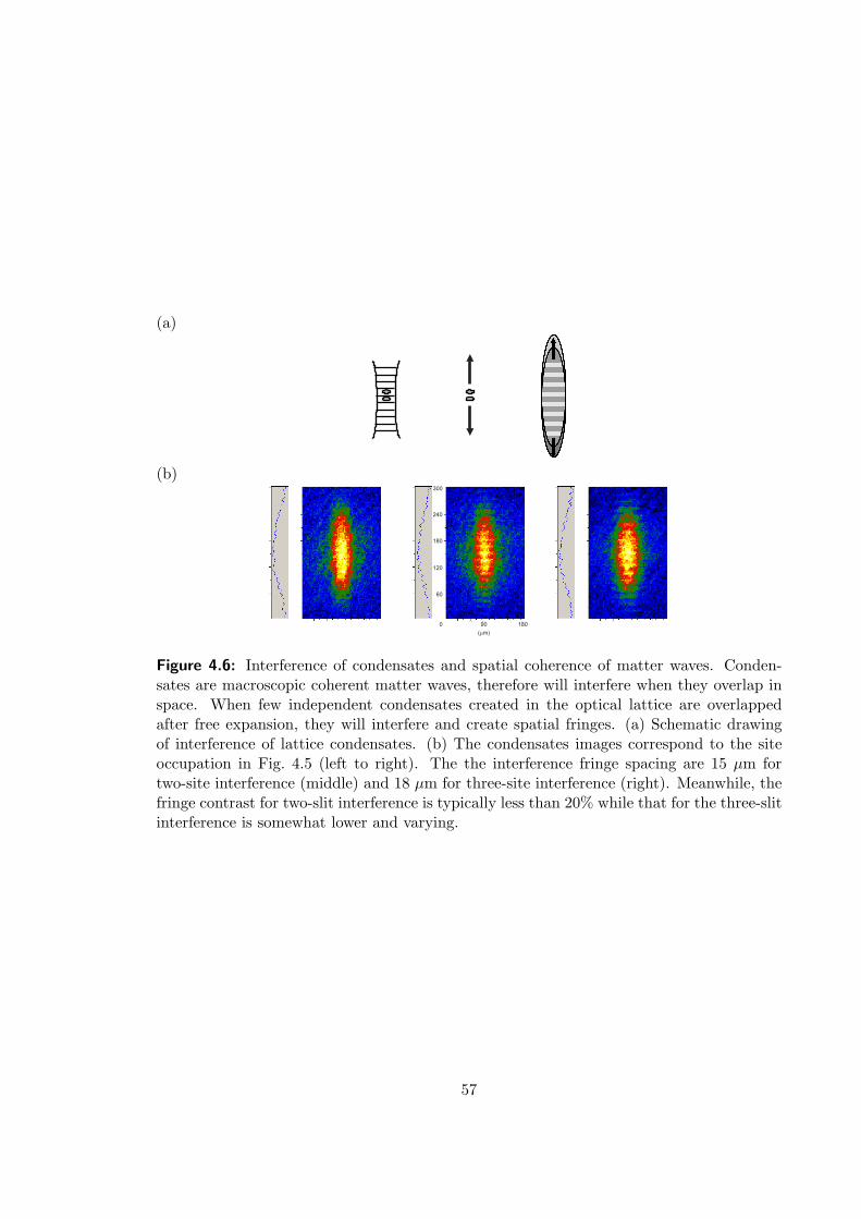
(a)

(b)

0

300

18090

60

120

180

240

( m)m

Figure 4.6: Interference of condensates and spatial coherence of matter waves. Conden-sates are macroscopic coherent matter waves, therefore will interfere when they overlap inspace. When few independent condensates created in the optical lattice are overlappedafter free expansion, they will interfere and create spatial fringes. (a) Schematic drawingof interference of lattice condensates. (b) The condensates images correspond to the siteoccupation in Fig. 4.5 (left to right). The the interference fringe spacing are 15 µm fortwo-site interference (middle) and 18 µm for three-site interference (right). Meanwhile, thefringe contrast for two-slit interference is typically less than 20% while that for the three-slitinterference is somewhat lower and varying.

57

Figure 4.7: Interference of 30,000 atoms in the |F = 1,mF = −1〉 state. In this case,the contrast of the interference is 80% and is much higher than in Fig. 4.6. This suggeststhe phase different among three spin components are different in different sites. The timeof flight is 26 ms, and the fringe spacing is measured to be 24 µm. The field of view is370×680 µm2.

The spacing resulting from two expanding condensates is given by the de Broglie wave-

length of the relative motion of the two independent condensates [10],

λrel =h

mvrel, (4.1)

where the relative velocity is determined by

vrel =d

τexp. (4.2)

Here d is the separation of the condensates, and for our experiment, the spacing of the

condensates is 5.3 µm (fixed by the standing wave). Given the expansion time τexp = 26 ms,

the relative velocity is calculated to be 200 µm/s, and the theoretical fringe spacing should

be 22.5 µm. The fringe spacing in Fig. 4.7 is measured to be 24 µm, which is in good

agreement with the theoretical prediction.

4.4 Bose Condensation in a Single Focus Trap

The key to reaching Bose condensation in an all-optical trap is efficient loading in a tight

confining potential for subsequent evaporative cooling. This understanding has led us to

create condensates in a cross trap and in a 1D lattice with an improved loading scheme.

The tight confinement in the cross trap and 1D lattice microtraps can lead to high densities

and high collision rates, however, the tight confinement will also cause a small trap volume.

58

This trap volume limitation has limited the initial number of atoms loaded into the trap,

and eventually limited the final condensate size to 30,000 atoms in both of the cross and

1-D lattice our optical traps. Therefore, a larger trap volume is desired for creating larger

stable condensates. A large-waist single focus trap is an ideal candidate as it is the simplest

trap geometry, and it provides relatively large trap volume. As shown in the first column

of Table 4.1, however, the initial loading number and collision rate in our single focus trap

are not sufficient to reach quantum degeneracy. In a recent experiment by Gennini et al., a

CO2 laser was strongly focused to a beam waist of 27 µm [82] from which a condensate was

created directly in the single focus trap. This tight trap loaded 4× 106 atoms with initial

density of 1 × 1013 cm−1, and phase space density of 1 × 10−4. A condensate of 12,000

atoms was created in their single-focus trap after 7 s of forced evaporation.

In a single focus trap, the trap volume scales strongly with the beam waist, or V ∝ w40,

where w0 is the beam waist at trap location. Meanwhile, mean trap frequency scales as ω ∝w−7/30 . Realizing a tight and large volume single focus optical trap seems contradictory at

first glance. However, we have learned from the 1D lattice condensate experiment that large

loading volume for efficient loading and tight confining potentials for efficient evaporative

cooling can be separated in time. Therefore, by varying the beam waist w0 in real time, it

is then possible to optimize both efficient loading and high collision rate in a single focus

trap. In particular, under adiabatic compression which is often true in an optical trap due

to its relatively high trap frequencies compared to the speed of compression, the density

and the elastic collision rate scale as n ∝ w−40 and γel ∝ w−5

0 , respectively.

The beam waist of a focused Gaussian beam is given by the formula, w0 = λ f/(πR),

where λ, f , and R are the wavelength, focal length of the lens, and input beam radius

respectively. Therefore, the beam waist can be varied by changing the R and/or f . We

chose to change the input beam size of the gaussian beam, for it can be easily achieved

via a zoom lens telescope. This trap compression technique was first developed by Weiss’s

group in a crossed YAG laser dipole trap [83], and we adopted this technique to compress

our single focus trap. As shown in Fig. 4.8.a, the optical trapping volume is maximized

by minimizing the CO2 beam diameter on the input side of the final lens (L3). The trap

59

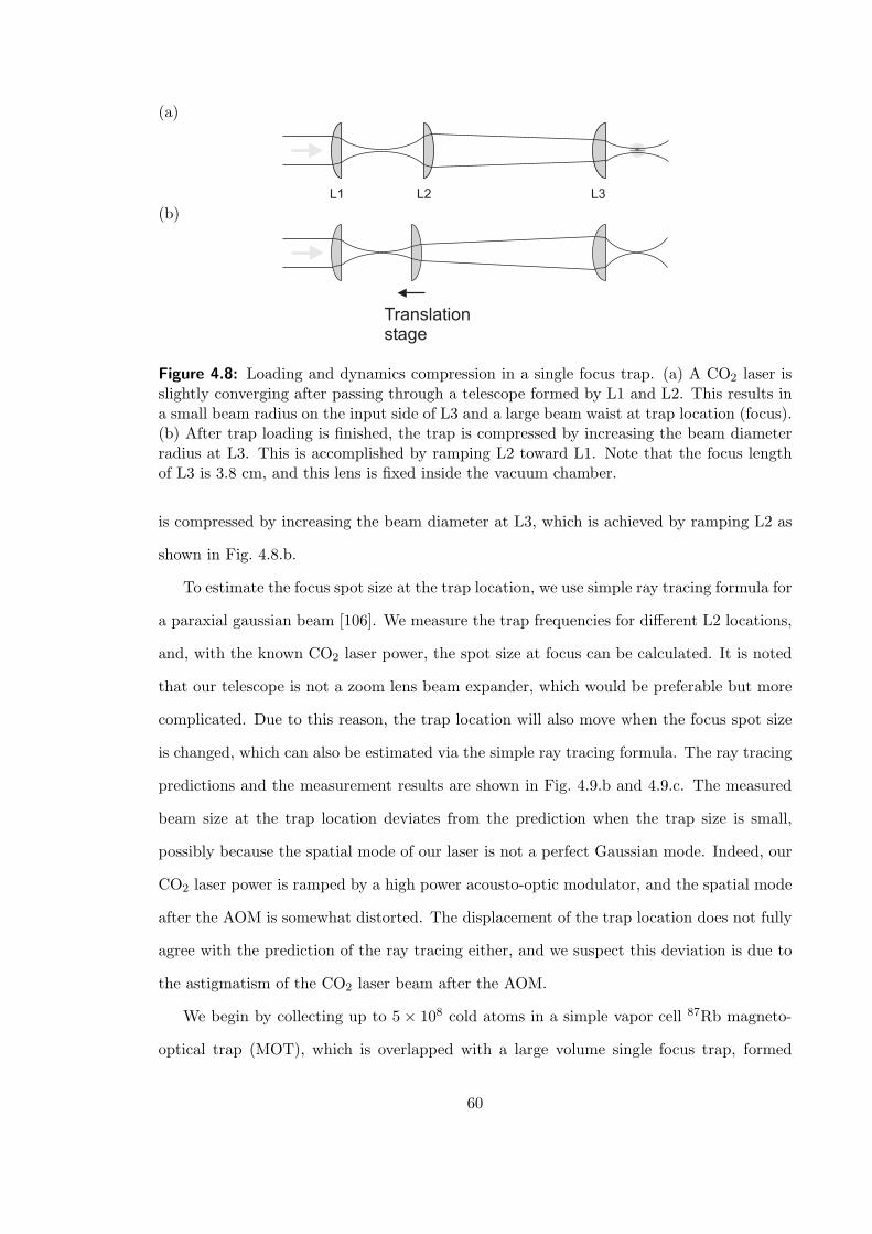
(a)

L1 L2 L3

(b)

Translationstage

Figure 4.8: Loading and dynamics compression in a single focus trap. (a) A CO2 laser isslightly converging after passing through a telescope formed by L1 and L2. This results ina small beam radius on the input side of L3 and a large beam waist at trap location (focus).(b) After trap loading is finished, the trap is compressed by increasing the beam diameterradius at L3. This is accomplished by ramping L2 toward L1. Note that the focus lengthof L3 is 3.8 cm, and this lens is fixed inside the vacuum chamber.

is compressed by increasing the beam diameter at L3, which is achieved by ramping L2 as

shown in Fig. 4.8.b.

To estimate the focus spot size at the trap location, we use simple ray tracing formula for

a paraxial gaussian beam [106]. We measure the trap frequencies for different L2 locations,

and, with the known CO2 laser power, the spot size at focus can be calculated. It is noted

that our telescope is not a zoom lens beam expander, which would be preferable but more

complicated. Due to this reason, the trap location will also move when the focus spot size

is changed, which can also be estimated via the simple ray tracing formula. The ray tracing

predictions and the measurement results are shown in Fig. 4.9.b and 4.9.c. The measured

beam size at the trap location deviates from the prediction when the trap size is small,

possibly because the spatial mode of our laser is not a perfect Gaussian mode. Indeed, our

CO2 laser power is ramped by a high power acousto-optic modulator, and the spatial mode

after the AOM is somewhat distorted. The displacement of the trap location does not fully

agree with the prediction of the ray tracing either, and we suspect this deviation is due to

the astigmatism of the CO2 laser beam after the AOM.

We begin by collecting up to 5 × 108 cold atoms in a simple vapor cell 87Rb magneto-

optical trap (MOT), which is overlapped with a large volume single focus trap, formed

60

(a)

10

8

6

4

2

0

L2

dis

pla

ce

me

nt

(mm

)

1.21.00.80.60.40.20.0

Time (s)

(b)

70

60

50

40

30

20

10

0

w0

(µm

)

1050-5-10L2 position (mm)

(c)

-500

0

500

Tra

p C

ente

r (

µm)

-10 -5 0 5 10L2 position (mm)

Figure 4.9: Geometrical parameters for dynamical trap compression. (a) shows the mea-sured position of Lens 2 (L2) vs. time for 10 mm displacement at a velocity of 10 mm/sand acceleration of 60 mm/s2. (b) shows the focused trap beam waist vs. L2 position. (c)shows the trap location displacement vs. L2 position. In Fig. (b) and (c), the solid curvesare the ray tracing predictions, and the solid circles are the measurement data. The beamwaists are calculated from the measured trap frequencies.

61

t = 0 0.6 s

2.8

mm

w0= 60 30 mm

Figure 4.10: Fluorescence images of trap loading and dynamical trap compression. A highpower CO2 laser is weakly focused to form a large volume dipole trap overlapping with theMOT. When the MOT is turned off, the trap is quickly compressed. The trap compressionoccurs in 600 ms, with a compression factor of 16. Note that, during the compression, a veryefficient cooling density enhancement is observed. In order to reduce the optical densityupon probing, during compressions, the cloud is allow to expand for longer times beforeprobing.

Figure 4.11: Growth of BEC in the single-focused trap vs. final CO2 laser power. At lowestfinal power, 40 mW, a mostly pure condensate of 300,000 atoms is created in the opticaltrap.

62

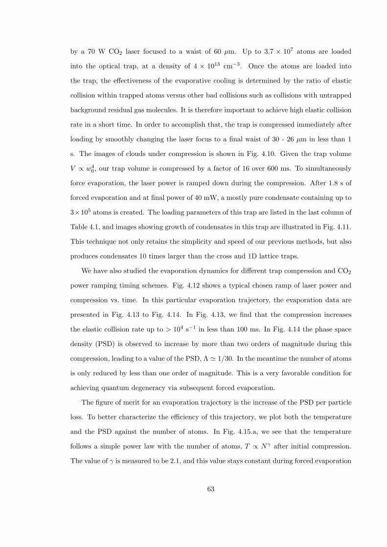
by a 70 W CO2 laser focused to a waist of 60 µm. Up to 3.7 × 107 atoms are loaded

into the optical trap, at a density of 4 × 1013 cm−3. Once the atoms are loaded into

the trap, the effectiveness of the evaporative cooling is determined by the ratio of elastic

collision within trapped atoms versus other bad collisions such as collisions with untrapped

background residual gas molecules. It is therefore important to achieve high elastic collision

rate in a short time. In order to accomplish that, the trap is compressed immediately after

loading by smoothly changing the laser focus to a final waist of 30 - 26 µm in less than 1

s. The images of clouds under compression is shown in Fig. 4.10. Given the trap volume

V ∝ w40, our trap volume is compressed by a factor of 16 over 600 ms. To simultaneously

force evaporation, the laser power is ramped down during the compression. After 1.8 s of

forced evaporation and at final power of 40 mW, a mostly pure condensate containing up to

3×105 atoms is created. The loading parameters of this trap are listed in the last column of

Table 4.1, and images showing growth of condensates in this trap are illustrated in Fig. 4.11.

This technique not only retains the simplicity and speed of our previous methods, but also

produces condensates 10 times larger than the cross and 1D lattice traps.

We have also studied the evaporation dynamics for different trap compression and CO2

power ramping timing schemes. Fig. 4.12 shows a typical chosen ramp of laser power and

compression vs. time. In this particular evaporation trajectory, the evaporation data are

presented in Fig. 4.13 to Fig. 4.14. In Fig. 4.13, we find that the compression increases

the elastic collision rate up to > 104 s−1 in less than 100 ms. In Fig. 4.14 the phase space

density (PSD) is observed to increase by more than two orders of magnitude during this

compression, leading to a value of the PSD, Λ ' 1/30. In the meantime the number of atoms

is only reduced by less than one order of magnitude. This is a very favorable condition for

achieving quantum degeneracy via subsequent forced evaporation.

The figure of merit for an evaporation trajectory is the increase of the PSD per particle

loss. To better characterize the efficiency of this trajectory, we plot both the temperature

and the PSD against the number of atoms. In Fig. 4.15.a, we see that the temperature

follows a simple power law with the number of atoms, T ∝ Nγ after initial compression.

The value of γ is measured to be 2.1, and this value stays constant during forced evaporation

63

0.01

0.1

1

10

100P

CO

2 (W

)

2.01.51.00.50.0Time (s)

70

60

50

40

30

20

10

w0 (µ

m)

PCO2

w0

10-6

10-5

10-4

10-3

Td

(K)

2.01.51.00.50.0Time (s)

10

2

46

100

2

46

1000

Ftrap (H

z)

Td

Ftrap

Figure 4.12: CO2 laser power and beam waist vs. time. An evaporation trajectory can betailored by varying the ramp of CO2 laser power (PCO2) and beam waist (w0). The leftplot shows a typical ramp, and the right plot shows the corresponding trap depth (TD) andmean trap frequency (Ftrap).

1013

2

4

6

810

14

2

n th

(1/c

m-3

)

2.01.51.00.50.0Time (s)

102

103

104

Γel (s

-1)

nth

Γel

10-7

10-6

10-5

10-4

10-3

T (

K)

2.01.51.00.5Time (s)

T TD

Figure 4.13: Density and elastic scattering rate vs. time. (Left) The trap compression leadsto thermal cloud density (nth), which further leads to high elastic collision rate (Γel) andefficient evaporative cooling. (Right) In the meantime, the fast dynamics enables a cloudto reach thermal equilibrium very quickly; temperature of the cloud basically follows thetrap depth with a scaling factor η = TD/T , where η ∼ 10. As can be seen The trappingpower stop ramp at 1.45 s, and without further ramping down the power, the temperaturequickly reaches a plateau.

64

(a)

68

106

2

4

68

107

2

N

2.01.51.00.50.0

Time (s)

10-4

10

-2 10

0 10

2 10

4 10

6

Λ

N Λ

Figure 4.14: Number (N) and phase space density (PSD, Λ) vs. time. The PSD increasessharply from 10−4 to 5 × 10−2 in the first 600 ms during which the trap compression andevaporation are taken place simultaneously. Condensate starts to appear at 1.5 s, and thenumber of Bose condensed atoms quickly reach a plateau of ≤ 300, 000 atoms at 1.8 s.Here, by definition, the PSD equals to the number of condensed atoms after the condensateemerges.

until the end of the power ramp. In Fig. 4.15.b, the PSD (Λ) also follows a simple power

law relationship with the number of atoms, or Λ ∝ Nρ. In the first regime where the elastic

collision rate is > 104 s−1, the increase of PSD does not cause much loss of particles, and the

exponent ρ1 = −5.2, which is close to the theoretical limit of a simple ergodical evaporation

model with ρ = 1− γ(ξ + 3/2) = −5.3, where ξ = 3/2 for 3D harmonic traps [107, 59, 24].

After the compression is finished, ρ = −2.8, which is somewhat smaller.

Our studies show that while the evaporation trajectory varies depending on the chosen

compression and power ramping scheme, evaporative cooling is relatively robust, and the

final number of Bose condensed atoms appeared to be relatively constant. The typical

number of condensed atoms is ∼ 1% of that initially loaded in the trap.

To summarize this chapter, we have extended the all-optical trapping technique to two

new trap geometries: a large-period 1D lattice and a large volume single-focus trap. The

common feature of the three trap geometries (including cross trap) are that they all achieve

efficient loading and tight confinement. These two conditions lead to highest spatial densities

(> 1014 cm−3) and high elastic collision rates (> 104 s−1), which further lead to efficient

evaporation with a typical evaporation time of less than 2 sec. In the 1D lattice geometry,

65

(a)

10-7

10-6

10-5

10-4

T (

K)

5 6 7 8 9

106

2 3 4 5 6 7 8 9

107

2 3

N

γ = 2.1

(b)

0.0001

0.001

0.01

0.1

1

Λ

6 7 8 9

106

2 3 4 5 6 7 8 9

107

2 3

N

ρ1 = −2.8

ρ2 = −5.2

Figure 4.15: Number and phase space density (PSD) vs. number of atoms. (a) Fit thetrajectory with a power law model, T = Nγ , we find γ = 2.1. (b) Similarly, fit thetrajectory with Λ = Nρ, we find the dynamics fall into two parameter regimes, ρ = −5.2and ρ2 = −2.8. Both arrows indicate the direction of time. Note that the error bars for thetemperature are too small to be resolved here.

66

interference between two independently trapped condensates are observed.

67

CHAPTER V

SPINOR CONDENSATE THEORY

Atomic Bose-Einstein condensates with internal spin degrees of freedom, so-called spinor

condensates, offer a new form of coherent matter with complex internal quantum structures.

Spinor condensates exhibit rich quantum dynamics due to the vector properties of the

condensate order parameter and the nonlinear spin-spin interactions.

Most current experiments employ magnetic trapping techniques in which the spin degree

of freedom is frozen, and BEC experiments in this type of trap mostly involve only one spin

component. Therefore, the order parameter of a one-component condensate is a scalar,

and its dynamics are restricted to the motional degrees of freedom, described by the scalar

Gross-Pitaevskii equation given in Eq. 1.1.

Stimulated by the early experiments by the JILA and MIT groups, and by the theoretical

work by Ho [39] and Ohmi and Machida [40], spinor condensates have been the subject of

many studies. Early experimental investigations of multi-component condensates have been

explored by utilizing two coupled hyperfine states in 87Rb [108, 109, 25, 110], and by F = 1

spinor condensates of Na by transferring spin polarized BEC made in magnetic traps into

far-off resonant optical traps [35]. The MIT group subsequently studied the ground state

properties of the spinor condensates and observed ground state domain structures [42],

metastable domains [52], and quantum spin tunneling [53].

The progress of spinor condensate theories is also impressive, and theoretical work has

covered ground state structure [39, 40, 111, 54, 112], quantum/coherent spin mixing [54,

113, 114, 115, 116, 117], spinor vortices [39, 40, 118], spin textures and domains [42, 119],

spin squeezing and entanglement [120, 121], and many other topics.

Here we focus on spin-1 condensates composed of the three spin components, mF = 0,±1

of the F = 1 hyperfine ground state (hereafter, denoted as m0,±1 states). At the microscopic

level, the interactions in spinor Bose gases are determined by two-body, s-wave collisions.

68

The mean-field interaction energy is V (r) = δ(r)(c0 + c2~Fa · ~Fb) [39, 40], where r is the

distance between two atoms a and b, and c0 and c2 characterize the strength of the scalar

and spin-dependent interactions respectively. These two mean-field interaction coefficients,

c0 and c2, are simple functions of the scattering lengths aF=0 and aF=2.

For the F = 1 hyperfine spinor in 87Rb, the spin-dependent mean-field energy |c2|nis only 200 pK [55, 56] for typical densities, n ∼ 1014 cm−3, which is much smaller than

both the scalar mean-field energy and the estimated temperature of the gas, ∼ 50 nK.

Nonetheless, the small spin-dependent mean field couplings are non-negligible and lead to

qualitatively different ground state structures depending on the sign of c2, being ferromag-

netic (c2 < 0) for 87Rb [55, 56, 44, 45] or anti-ferromagnetic (c2 > 0) for 23Na [42, 122].

Moreover, these spinor interactions yield a rich variety of coherent and incoherent phe-

nomena including coherent spinor mixing, spin squeezing and entanglement [54, 120], spin

domain formation, and spinor vortices.

In this chapter, the microscopic theory for spinor condensates will be briefly reviewed.

The theoretical approach in this chapter follows closely to ref. [39, 123, 54].

5.1 Microscopic picture

The atomic interactions in spinor condensates are dominated by two-body s-wave collisions.

The microscopic picture of an ultracold collision of two identical bosonic spinors is illustrated

in Fig. 5.1. When two atoms approach each other, their spins will temporarily couple

together to form a total spin, and the two atomic spins precess around this total spin

during the collision. After the collision, the two spins decouple and the atoms move away

from each other. For two identical spin-f particles, the total spin is given by ~F = ~f1 +~f2,

and the allowed total spins are F = 2f, 2f − 1, · · · , 0. However, due to the symmetry

(anti-symmetry) required by identical bosons (fermions), only F = even (odd) channels

are allowed for bosons (fermions), when the total spatial wavefunction of the two atoms is

symmetric. Here we focus on spin-1 condensates, thus the allowed collision channels are

F = 2, 0, and two atomic parameters are required to describe the interactions, i.e., s-wave

scattering lengths, aF=2 and aF=0 for total spin 2 and 0 channels.

69

F=2,0

f=1

f=1

Figure 5.1: Intuitive picture of atomic interactions in spinor condensates: binary collisionof spin-1 bosons. (Left) Two spin-1 bosons approach each other. (Center) The atomic spinof two bosons couple to form a total spin, and then the bosons precess around this totalspin during the collision. The total spin can be F = 2, 0. (Right) Two bosons break apartafter collision is finished.

By projecting the joint space of two spin-1 bosons,∑

mf|f = 1,mf 〉⊗

∑mf|f = 1, mf 〉,

to the joint space of the irreducible total spin spaces,∑

mF|F = 0,mF 〉⊗

∑mF

|F = 2,mF 〉,the binary interaction can be decomposed into contributions from the different total spin

channels,

V (~r1 − ~r2) = δ(~r1 − ~r2)2f∑

F=0

gFPF . (5.1)

The coupling strength gF is

gF =4π~2aF

m, (5.2)

where aF is the s-wave scattering length for total spin-F channel, and m is the atomic mass.

The projection operator PF is

PF ≡F∑

mF =−F

|F, mF 〉〈F,mF |. (5.3)

For identical bosons, the allowed total spins are F = even (see Appendix B), and the

projection operators satisfy the following closure relationship:

1 =2f∑

F=0,even

PF = P0 + P2 + · · · . (5.4)

Meanwhile, the spin-spin coupling of two spin-f bosons can be found using the identity:

~f1 ·~f2 =F2 − f2

1 − f22

2=

F (F + 1)− 2f(f + 1)2

. (5.5)

Here ~f1, ~f2, and ~F are dimensionless.

Applying the identity operator leads to

~f1 ·~f2 = (~f1 ·~f2)1 =∑

f

~f1 ·~f2PF =∑

F

λFPF , (5.6)

70

where λF = F (F+1)−2f(f+1)2 . For spin-1 condensates,

1 = P0 + P2, (5.7)

and

~f1 ·~f2 = P2 − 2P0. (5.8)

By the aid of the above two identities and Eq. (5.1), the binary interactions for identical

spin-1 bosons can be expressed as

V (~r1 − ~r2) = δ(~r1 − ~r2)2∑

f=0

gfPf (5.9a)

= δ(~r1 − ~r2)(g0P0 + g2P2) (5.9b)

= δ(~r1 − ~r2)(c0(P0 + P2) + c2(P2 − 2P0)) (5.9c)

= δ(~r1 − ~r2)(c0 + c2~f1 ·~f2). (5.9d)

Here c0 and c2 are density- and spin-dependent interactions, c0 and c2, with

c0 =g0 + 2g2

3=

4π~2

ma, (5.10)

and

c2 =g2 − g0

3=

4π~2

m

∆a

3. (5.11)

In the above expressions a = (aF=0 + 2aF=2)/3 is the mean s-wave scattering length, and

∆a = aF=2 − aF=0 is the scattering length difference.

The total Hamiltonian for a spin-1 condensate is

H =N∑

i=1

p2i

2m+ U(ri) +

∑

i<j

V (~ri − ~rj) (5.12a)

=N∑

i=1

p2i

2m+ U(ri) +

∑

i<j

δ(ri − rj)(c0 + c2~fi ·~fj). (5.12b)

Here, U(~r) is the total external potentials, which includes the optical trapping potential

and the Zeeman energy due to external magnetic fields.

An immediate important feature of a spinor system is that the spin-spin interaction is

invariant under rotation in spin space. This rotation symmetry leads to a vectorial order

71

ferromagnetic anti-ferromagnetic

c2< 0 c

2> 0

Figure 5.2: Magnetic nature of spin-1 condensates.

parameter [39]. Secondly, although typically |c2| ¿ c0 due to that aF=2 ' aF=0 [56, 42],

it is responsible for coupling different Zeeman states. Indeed, it is this coupling that leads

to spinor dynamics such as spin mixing and spin domain formation. Finally, the sign of

c2 determines the ground state structure, as well as the dynamical properties of the spinor

condensates.

As illustrated in Fig. 5.2, spin-1 condensates are divided into two categories depending

on the sign of c2. When c2 < 0, maximizing ~fi ·~fj and consequently minimizing H requires

that spinors are all polarized in the same direction, which is equivalent to |f = 1,mf = 1〉state under spin rotation. Therefore, it is said to be ferromagnetic. In contrast, when

c2 > 0, the ground state is said to be anti-ferromagnetic, since spinors align in opposite

directions, which is a singlet state [54, 39, 111].

5.2 Second Quantized Hamiltonian for Spin-1 Condensates

It is natural to describe this many-body system in the second quantized formalism. Ad-

ditionally, as will be seen immediately, simplification of spinor dynamics due to rotational

symmetry can be better appreciated in the second quantized formalism. In terms of the

field operators of three Zeeman states, (Ψ1,Ψ0,Ψ−1), the most general spin-1 Hamiltonian

is given by [39][40]

H =∫

d3rΨ†i (~r)(−

~2∇2

2mδij + Uij(~r))Ψj(~r)

+gij,kl

2

∫d3r1d3r2Ψ

†i (~r1)Ψ

†j(~r2)Ψk(~r2)Ψl(~r1)δ(~r1 − ~r2). (5.13)

72

Here, δij is the Kronecker delta function, and Uij ’s are the external potentials. The Uij ’s

allow nonzero coupling between different Zeeman states, such as the coupling between two

Zeeman states by radio frequency (RF) waves. The indices i, j, k, l run through all three

Zeeman states, 1, 0,−1, and the sum over repeated indices is implied. The coefficients

gij,kl are the coupling constants for collision channels k, l → i, j, and in the most general

case, there are (2f + 1)4 = 34 = 81 gij,kl’s for spin-1 condensates. This large number of

independent g’s, however, can be greatly reduced as the collisions are symmetric under

exchange of particles (gij,kl = gji,kl) and time-reversal (gij,kl = gkl,ij). This value is then

reduced to (l2 + l)(l2 + l + 2)/8, where l = 2f + 1 (see Appendix B). For spin-1 systems,

the number of independent g’s is 21, which is still a large number. However, due to the

spin rotational symmetry, the number of free parameters can be ultimately reduced to only

two atomic parameters, the s-wave scattering lengths for total spin-2 and spin-0 collision

channels, aF=2 and aF=0. Recall the results from the last section, simply express Eq. (5.12)

in the 2nd quantized format, and Eq. (5.13) is immediately reduced to

H =∫

d3rΨ†i (~r)[−

~2∇2

2mδij + Uij(~r)]Ψj(~r)

+c0

2

∫d3rΨ†

i (~r)Ψ†j(~r)Ψj(~r)Ψi(~r)

+c2

2

∫d3rΨ†

i (~r)Ψ†j(~r)~fjk ·~filΨk(~r)Ψl(~r). (5.14)

Here, c0 and c2 are the density- and spin-dependent coupling strengthes for spinors defined

in Eq. (5.10) and (5.11), and ~fjk · ~fil = (fα)jk(fα)il , where (fα)jk are the matrix elements

for three Cartesian, traceless spin-1 Pauli matrices,

fx =1√2

0 1 0

1 0 1

0 1 0

, fy =i√2

0 −1 0

1 0 −1

0 1 0

, fz =

1 0 0

0 0 0

0 0 −1

. (5.15)

The second and third integrals in Eq. (5.14) represent the nonlinear atom-atom interactions,

and they constitute the interaction Hamiltonian,

Hint =12

∫d3rc0(Ψ

†iΨ

†jΨjΨi) + c2(Ψ

†iΨ

†j(~fjk ·~fil)ΨkΨl). (5.16)

73

Table 5.1: Table of two-body interaction strengths. Upper table lists the intra- andinter-state particle exchange collisions. Lower table lists the spin changing or spin mixingcollisions.

gij,ji m1 m0 m−1

m1 c0 + c2c0+c2

2c0−c2

2

m0c0+c2

2 c0c0+c2

2

m−1c0−c2

2c0+c2

2 c0 + c2

g1−1,00 c2

g00,1−1 c2

We can express this interaction Hamiltonian in terms of three spin components explicitly

(see Appendix C),

Hint =12

∫d3r(c0 + c2)Ψ

†1Ψ

†1Ψ1Ψ1 + c0Ψ

†0Ψ

†0Ψ0Ψ0 + (c0 + c2)Ψ

†−1Ψ

†−1Ψ−1Ψ−1

+2(c0 + c2)Ψ†1Ψ

†0Ψ0Ψ1 + 2(c0 − c2)Ψ

†1Ψ

†−1Ψ−1Ψ1 + 2(c0 + c2)Ψ

†0Ψ

†−1Ψ−1Ψ0

+2c2Ψ†−1Ψ

†1Ψ0Ψ0 + 2c2Ψ

†0Ψ

†0Ψ−1Ψ1. (5.17)

In this interaction Hamiltonian, the first three terms represent the intra-state collisions,

or the self-scattering, the following three terms represent the inter-state collisions or the

cross-scattering, and the last two terms stand for the spin mixing, which provide a way

to relax to the spinor ground state under the presence of dissipation when the initial spin

populations are not in their minimal energy configuration. The coupling strength coefficients

are tabulated in Table 5.1.

5.3 Spinors In Magnetic Fields

Is is important to understand the interactions between a spinor condensate and external

magnetic fields. Since spin interactions are magnetic interactions, external magnetic fields

will compete with, or even dominate the internal spin interactions. First, an external

magnetic field will break rotational symmetry along the axis defined by that field [39]. A

homogeneous field will change the total Zeeman energy of a spinor condensate and subse-

quently alter its ground state spin configuration. A homogeneous field will also cause spinors

74

to undergo Larmor precessions around the z axis, which results in fast rotation of spinor’s

phase and affects phase sensitive dynamics. An inhomogeneous field will exert magnetic

forces on spinors and can cause phase separation of different spin states. In addition, field

inhomogeneities will give rise to spatial dephasing of coherent spinor dynamics. Finally, AC

magnetic fields can cause diabatic spin flips in a low bias field.

In a static B field, the Zeeman energy of the spin states is given by

EZ =

E1 0 0

0 E0 0

0 0 E−1

(5.18)

Typically, the spin-dependent interactions are Eint/h < 10 Hz for a typical density of

1014 cm−3. In principle, to observe spinor dynamics, the external Zeeman effects introduced

by the external field should be much less than 10 Hz, which requires zeroing the B field

to micro-Gauss regime. However, due to the conservation of magnetization, which will be

explained in the next few paragraphs, one can still observe interesting spinor dynamics in

the milli-Gauss to Gauss regime.

The mean-field global ground state for ferromagnetic (anti-ferromagnetic) spinors is

|F = 1,mF = 1〉 (|F = 1,mF = 0〉) state [39]. If a spinor condensate forms with a non-

equilibrium spin configuration and a net magnetization, M = ρ1 − ρ−1, where ρ±1 are the

fractional population of mF = ±1 states, then the condensate can only relax to its global

ground state via spin non-conserved collisions. This is, however, not allowed because the

fundamental atomic collisions conserve the total spin (angular momentum), which is clearly

shown in Eq. (5.17). Therefore, in a spin-independent trap, the total magnetization of a

spinor condensate should be a conserved quantity.

The non-spin mixing collisions in the interacting Hamiltonian do not cause a change of

populations in different spin states, and therefore will not change the Zeeman energy of the

condensate in a B field. In contrast, spin changing collisions (spin mixing) will cause change

of spin populations and the total magnetic energy. The spin-changing collisions read

2|mF = 0〉 ←→ |mF = 1〉+ |mF = −1〉. (5.19)

75

The change of magnetic energy per particle in this reaction process going to the right

is δ = (E1 + E−1 − 2E0)/2 > 0. This energy difference therefore energetically favors

the direction of the arrow going to the left. Due to the conservation of magnetization, δ

essentially cancels the linear Zeeman effect, η = (E−1 −E1)/2, resulting in a much smaller

Zeeman effect. According to the Breit-Rabi formula, or Eq. (2.1), δ ' g2Jµ2

BB2/16Ehfs,

where gJ , µB, B, and Ehfs are the Lande g-factor for electron, Bohr magneton, magnetic

field, and hyperfine splitting. For 87Rb δ ' B2× 71.6 Hz/G2, and δ vs. B field is plotted in

Fig. 5.3(a). In a field between 0.001 and 1 G, δ is 4 to 6 orders of magnitude smaller than

η as shown in Fig. 5.2(b). In a typical field of 100 mG, δ '0.7 Hz, which is small compared

to the spinor energy (. 10 Hz). Indeed, it is the conservation of magnetization that leads

to cancellation of linear Zeeman shifts and allows observation of spinor dynamics in a field

regime much higher than a few micro-Gauss.

5.4 Coupled Gross-Pitaevskii equations for spin-1 conden-sates

The dynamics of spinor condensates are governed by the coupled spin-1 Gross-Pitaevskii

(GP) equation for the three spin states. These coupled equations of motion for spin-1 fields

can be derived by the Heisenberg equation of motion,

i~∂Ψα

∂t= [Ψα,H], α = 1, 0,−1. (5.20)

Substituting Eq. (5.14) into Eq. (5.20), and after some calculation, the coupled equations

of motion for spin-1 fields are given by

i~∂Ψα

∂t= (

−~2

2m∇2 + Uα)Ψα + c0Ψ

†iΨiΨα + c2Ψ

†j~Fαk · ~FjlΨlΨk, α = 1, 0,−1. (5.21)

Here Uα is the external potentials including the trapping potential and the Zeeman energies,

and we assume Uα is diagonal.

In the mean-field limit in which the ground state is macroscopically occupied, one can

replace three spinor field operators with a 3-component vectorial order parameter for this

ground state and ignore the contribution from excited states (due to quantum fluctuations),

76

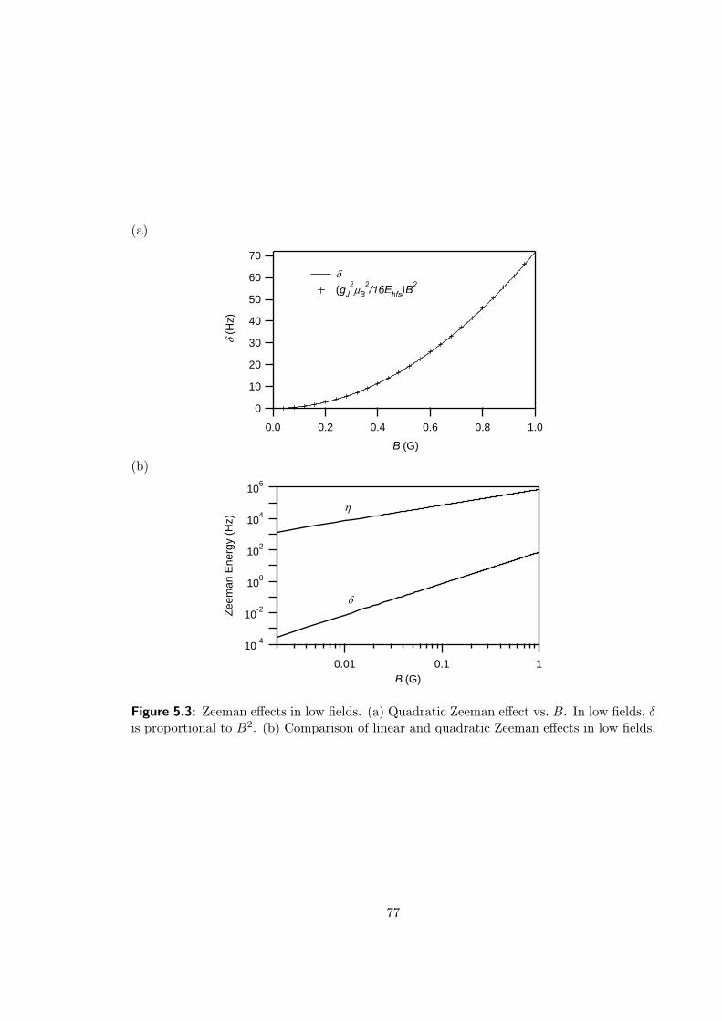
(a)

70

60

50

40

30

20

10

0

d (

Hz)

1.00.80.60.40.20.0

B (G)

d

(gJ

2mB

2/16Ehfs)B

2

(b)

10-4

10

-2

10

0

10

2

104

106

Zee

man

Ene

rgy

(Hz)

0.01 0.1 1B (G)

h

d

Figure 5.3: Zeeman effects in low fields. (a) Quadratic Zeeman effect vs. B. In low fields, δis proportional to B2. (b) Comparison of linear and quadratic Zeeman effects in low fields.

77

i.e.,

(ψ1, ψ0, ψ−1)T = 〈(Ψ1,Ψ0,Ψ−1)T 〉, (5.22a)

(ψ∗1, ψ∗0, ψ

∗−1)

T = 〈(Ψ†1,Ψ

†0,Ψ

†−1)

T 〉. (5.22b)

Then the three coupled Gross-Pitaevskii equations for spin-1 order parameters are given by

i~∂ψ1

∂t= L1ψ1 + c0nψ1 + c2(n1 + n0 − n−1)ψ1 + c2ψ

∗−1ψ0ψ0, (5.23a)

i~∂ψ0

∂t= L0ψ0 + c0nψ0 + c2(n1 + n−1)ψ0 + 2c2ψ

∗0ψ1ψ−1, (5.23b)

i~∂ψ−1

∂t= L−1ψ−1 + c0nψ−1 + c2(n−1 + n0 − n1)ψ−1 + c2ψ

∗1ψ0ψ0, (5.23c)

where L±1,0 ≡ (−~2∇2

2m + U±1,0), n = n1 + n0 + n−1 is the total density, and ni = |ψi|2 is

the density for each spin component.

The penultimate term in Eq. (5.23a-c) results in the cross-phase modulation, which

drives spatial dynamics that can ultimately lead to spin domain formation. The last term

in Eq. (5.23a-c) represent the coherent spin mixing, which can result in oscillations of the

spin populations when the spinor condensate is not in the spinor ground state. These

two processes occur with the same time scale (typically < 10 Hz for 87Rb), and they are

both very sensitive to external magnetic fields and field gradients represented in E±1,0

[42, 111, 124, 44, 45, 125, 117]. Therefore, the two dynamics are generally inseparable, and

the interplay of the two processes reveal a rich coupling between the internal and external

degrees of freedom of the condensate components which resulting in a variety of observed

phenomena including spin mixing [42, 44, 45], spin domain formation [42], and spin textures

[118, 126].

5.5 Single-Mode approximation

Although the internal and external dynamics are generally inseparable, under certain condi-

tions they can be decoupled. In particular, when the available spin interaction energy is less

than that required to create spatial spin structures in the condensates, then the external

dynamics will be suppressed. This occurs when the spin healing length ξs = h/√

2m |c2|n

78

is larger than the size of the condensate. In this case, then ψ1, ψ0 and ψ−1 share the same

spatial wave function and allows separation of spatial dynamics and the internal spinor dy-

namics. This is known as the single-mode approximation (SMA) and leads to considerable

simplification of Eq. (5.23).

Under SMA, the vectorial order parameter can be written as

~ψi(~r) =√

Nφ(~r)e−iµt/~~ζ(t), (5.24)

where N is the total number of atoms, φ(r) is the common spatial mode function, µ is the

chemical potential, and ~ζ = (ζ1, ζ0, ζ−1)T is the internal state vector with |~ζ|2 = 1. The

mode function φ(~r) satisfies the normalization condition∫ |φ(~r)|2d3r = 1, and its dynamics

is determined by the spin-independent Hamiltonian, Hs = −(~2/2m)∇2 + U + c0n, as

discussed in ref. [54, 114, 127].

Substituting the single-mode spinor wavefunctions into the Gross-Pitaevskii equations

to eliminate the spatial dynamics via Hsφ(~r) = µφ(~r), and integrating over coordinate

space, we arrive at the coupled spinor equations,

i~ζ1 = E1ζ1 + c [(ρ1 + ρ0 − ρ−1)] ζ1 + ζ20ζ∗−1, (5.25a)

i~ζ0 = E0ζ0 + c [(ρ1 + ρ−1] ζ0 + 2ζ1ζ−1ζ∗0 , (5.25b)

i~ζ−1 = E−1ζ−1 + c [(ρ−1 + ρ0 − ρ1)] ζ−1 + ζ20ζ∗1 , (5.25c)

where c = c2N∫ |φ(~r)|4d3r is the averaged (integrated) spin mean-field for the whole

condensate, and ρi = |ζi|2 is the fractional population of ith spin state.

The normalization condition,∑3

i=1 ρi = 1, and conservation of magnetization, M =

ρ1 − ρ−1, can be used to further simplify Eq. (5.25). Indeed, Eq. (5.25) can be reduced by

transforming ζ±1 → ζ±1 exp [−i(E0 ∓ η)t/~] and ζ0 = ζ0 exp [−iE0t/~] with ζi =√

ρie−iθi .

Under the constraints and this transformation, the internal spinor dynamics take on a

particularly simple form, and are determined by just two dynamical variables, ρ0(t), the

fractional population of the m0 state, and the relative phase of the spinor components

79

θ = θ1 + θ−1 − 2θ0:

ρ0 =2c

~ρ0

√(1− ρ0)2 −M2 sin θ, (5.26)

θ = −2δ

~+

2c

~

[(1− 2ρ0) +

(1− ρ0)(1− 2ρ0)−M2

√(1− ρ0)2 −M2

cos θ

], (5.27)

where η = (E−1−E1)/2 and δ = (E1 + E−1− 2E0)/2 are the linear and quadratic Zeeman

shifts. These two equations represent a classical nonlinear pendulum, with the total energy

(Hamiltonian)

E = cρ0

[(1− ρ0) +

√(1− ρ0)2 −M2 cos θ

]+ δ(1− ρ0). (5.28)

It is noted that Eq. (5.26) and (5.27) can also be derived by ρ0 = −(2/~)∂E/∂θ and θ =

(2/~)∂E/∂ρ0. These coupled equations also represent a type of nonlinear Josephson oscilla-

tor and point to the equivalency of spin mixing in a spin-1 condensate to Josephson systems

realized in superconductors [128] and other superfluids [46, 47, 129, 12, 109, 130, 131, 104].

The non-linearity of these equations provides a rich manifold of dynamical trajectories that

can be accessed experimentally by choice of initial populations and phases of the spin com-

ponents and the strength of the applied magnetic field. Experimental studies of the coherent

spin mixing described here will be presented in Chapter 7.

80

CHAPTER VI

OBSERVATION OF SPINOR DYNAMICS IN F=1 AND

F=2 BOSE CONDENSATES

In this chapter, we describe our experimental investigation of the spin dynamics and

ground state properties of 87Rb spinor condensates in an all-optical trap, starting with

well-characterized initial conditions in a known magnetic field. We focus on the F = 1

case and confirm the predicted ferromagnetic behavior. We observe evidence of popula-

tion oscillation between different spin states during the spin mixing and observe reduced

magnetization fluctuations, pointing the way to future exploration of the underlying spin

squeezing and spin entanglement predicted for the system [132]. We also create F = 2

spinors using a microwave excitation and measure a decay of the condensate with a time

constant of 250 ms. Despite the short lifetime, spin mixing of the spin-2 condensates is

observed within 50 ms.

Depending on the scattering lengths in different angular momentum channels, F = 1

spinor condensates can be either ferromagnetic or anti-ferromagnetic [39], and the corre-

sponding ground state structure and dynamical properties of the two cases are very distinct.

While the Na F = 1 spinor is anti-ferromagnetic, the 87Rb F = 1 spinor is ferromagnetic in

nature [55][56]. Hence, our all-optical route to BEC provides an excellent opportunity for

initial exploration of ferromagnetic spinor quantum gases.

6.1 Formation of Spinor Condensates

An optical trap can be essentially spin independent for large enough detunings and is ideally

suited for the studies of spinor condensates. The spin degrees of freedom are unconstrained

in an optical trap, and therefore spinor condensates can naturally form in the optical trap.

To observe spinor condensates, we perform time-of-flight expansion in a Stern-Gerlach type

81

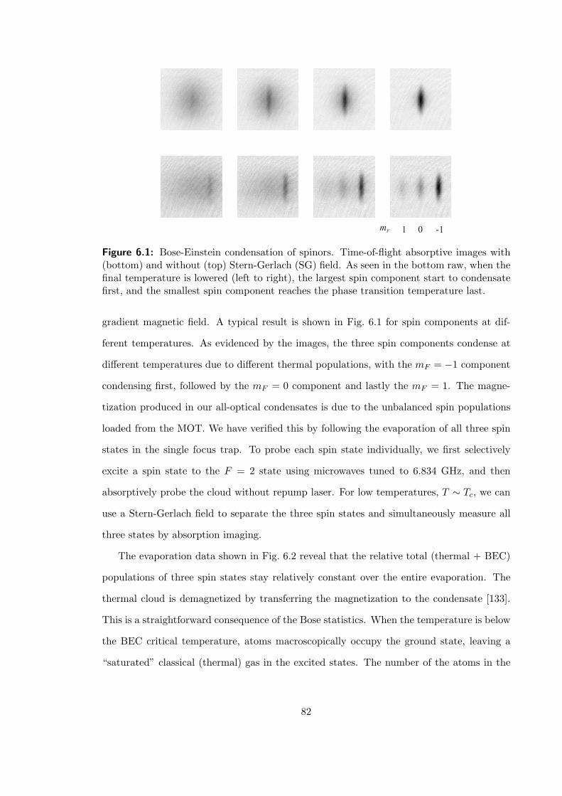
1 0 -1mF

Figure 6.1: Bose-Einstein condensation of spinors. Time-of-flight absorptive images with(bottom) and without (top) Stern-Gerlach (SG) field. As seen in the bottom raw, when thefinal temperature is lowered (left to right), the largest spin component start to condensatefirst, and the smallest spin component reaches the phase transition temperature last.

gradient magnetic field. A typical result is shown in Fig. 6.1 for spin components at dif-

ferent temperatures. As evidenced by the images, the three spin components condense at

different temperatures due to different thermal populations, with the mF = −1 component

condensing first, followed by the mF = 0 component and lastly the mF = 1. The magne-

tization produced in our all-optical condensates is due to the unbalanced spin populations

loaded from the MOT. We have verified this by following the evaporation of all three spin

states in the single focus trap. To probe each spin state individually, we first selectively

excite a spin state to the F = 2 state using microwaves tuned to 6.834 GHz, and then

absorptively probe the cloud without repump laser. For low temperatures, T ∼ Tc, we can

use a Stern-Gerlach field to separate the three spin states and simultaneously measure all

three states by absorption imaging.

The evaporation data shown in Fig. 6.2 reveal that the relative total (thermal + BEC)

populations of three spin states stay relatively constant over the entire evaporation. The

thermal cloud is demagnetized by transferring the magnetization to the condensate [133].

This is a straightforward consequence of the Bose statistics. When the temperature is below

the BEC critical temperature, atoms macroscopically occupy the ground state, leaving a

“saturated” classical (thermal) gas in the excited states. The number of the atoms in the

82

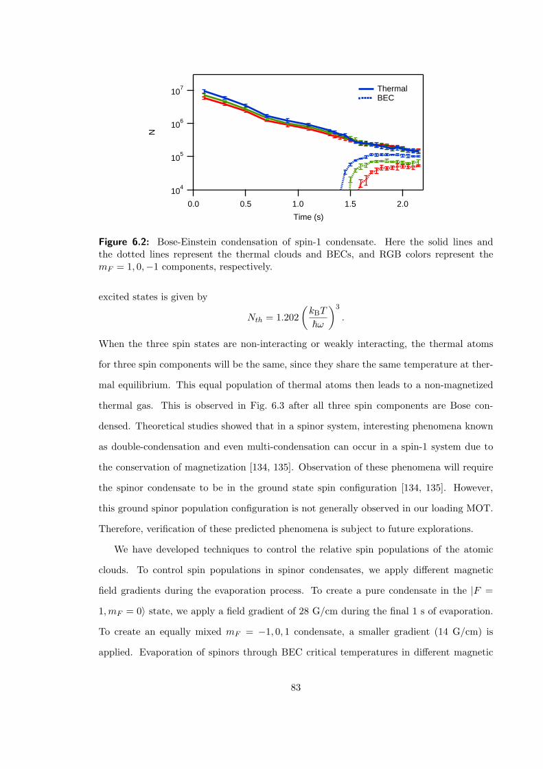
104

105

106

107

N

2.01.51.00.50.0

Time (s)

Thermal BEC

Figure 6.2: Bose-Einstein condensation of spin-1 condensate. Here the solid lines andthe dotted lines represent the thermal clouds and BECs, and RGB colors represent themF = 1, 0,−1 components, respectively.

excited states is given by

Nth = 1.202(

kBT

~ω

)3

.

When the three spin states are non-interacting or weakly interacting, the thermal atoms

for three spin components will be the same, since they share the same temperature at ther-

mal equilibrium. This equal population of thermal atoms then leads to a non-magnetized

thermal gas. This is observed in Fig. 6.3 after all three spin components are Bose con-

densed. Theoretical studies showed that in a spinor system, interesting phenomena known

as double-condensation and even multi-condensation can occur in a spin-1 system due to

the conservation of magnetization [134, 135]. Observation of these phenomena will require

the spinor condensate to be in the ground state spin configuration [134, 135]. However,

this ground spinor population configuration is not generally observed in our loading MOT.

Therefore, verification of these predicted phenomena is subject to future explorations.

We have developed techniques to control the relative spin populations of the atomic

clouds. To control spin populations in spinor condensates, we apply different magnetic

field gradients during the evaporation process. To create a pure condensate in the |F =

1,mF = 0〉 state, we apply a field gradient of 28 G/cm during the final 1 s of evaporation.

To create an equally mixed mF = −1, 0, 1 condensate, a smaller gradient (14 G/cm) is

applied. Evaporation of spinors through BEC critical temperatures in different magnetic

83

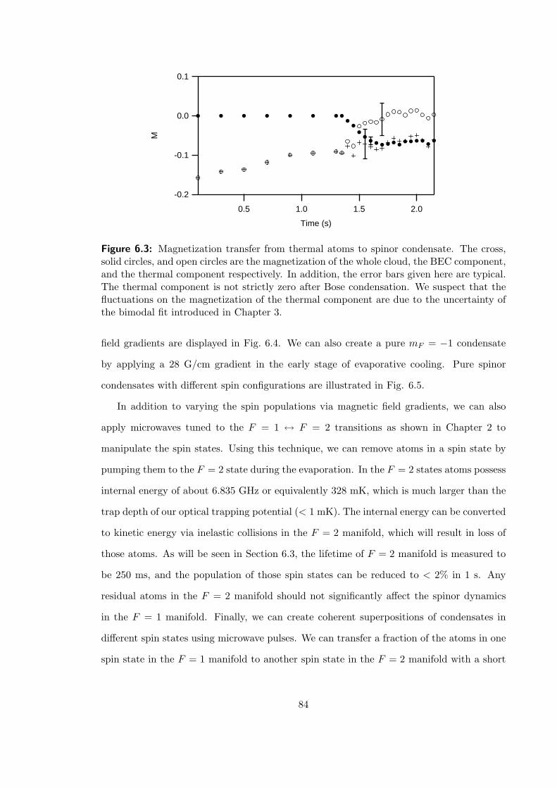
-0.2

-0.1

0.0

0.1

M

2.01.51.00.5

Time (s)

Figure 6.3: Magnetization transfer from thermal atoms to spinor condensate. The cross,solid circles, and open circles are the magnetization of the whole cloud, the BEC component,and the thermal component respectively. In addition, the error bars given here are typical.The thermal component is not strictly zero after Bose condensation. We suspect that thefluctuations on the magnetization of the thermal component are due to the uncertainty ofthe bimodal fit introduced in Chapter 3.

field gradients are displayed in Fig. 6.4. We can also create a pure mF = −1 condensate

by applying a 28 G/cm gradient in the early stage of evaporative cooling. Pure spinor

condensates with different spin configurations are illustrated in Fig. 6.5.

In addition to varying the spin populations via magnetic field gradients, we can also

apply microwaves tuned to the F = 1 ↔ F = 2 transitions as shown in Chapter 2 to

manipulate the spin states. Using this technique, we can remove atoms in a spin state by

pumping them to the F = 2 state during the evaporation. In the F = 2 states atoms possess

internal energy of about 6.835 GHz or equivalently 328 mK, which is much larger than the

trap depth of our optical trapping potential (< 1 mK). The internal energy can be converted

to kinetic energy via inelastic collisions in the F = 2 manifold, which will result in loss of

those atoms. As will be seen in Section 6.3, the lifetime of F = 2 manifold is measured to

be 250 ms, and the population of those spin states can be reduced to < 2% in 1 s. Any

residual atoms in the F = 2 manifold should not significantly affect the spinor dynamics

in the F = 1 manifold. Finally, we can create coherent superpositions of condensates in

different spin states using microwave pulses. We can transfer a fraction of the atoms in one

spin state in the F = 1 manifold to another spin state in the F = 2 manifold with a short

84

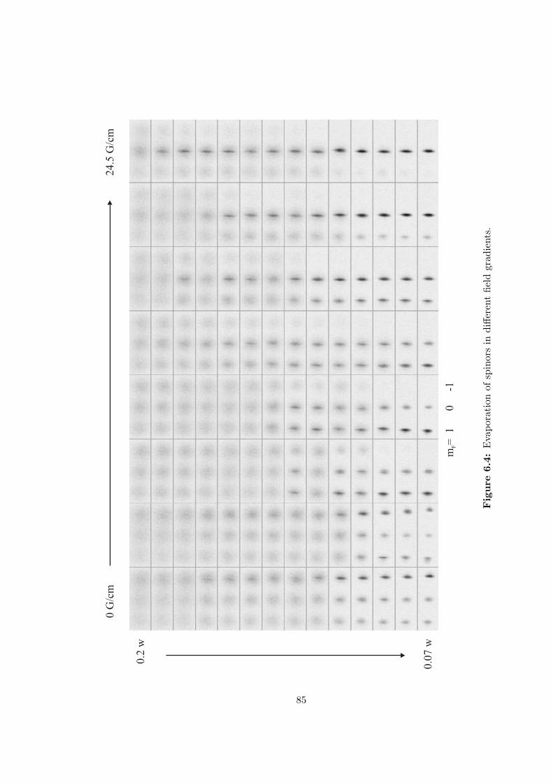
0.2

w

0.0

7 w

0 G

/cm

24.5

G/c

m

m=

1 0 -

1F

Fig

ure

6.4:

Eva

pora

tion

ofsp

inor

sin

diffe

rent

field

grad

ient

s.

85

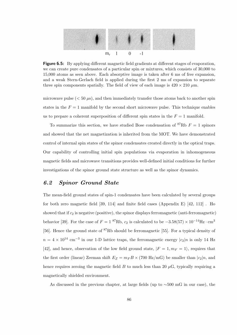
mF 01 -1

Figure 6.5: By applying different magnetic field gradients at different stages of evaporation,we can create pure condensates of a particular spin or mixtures, which consists of 30,000 to15,000 atoms as seen above. Each absorptive image is taken after 6 ms of free expansion,and a weak Stern-Gerlach field is applied during the first 2 ms of expansion to separatethree spin components spatially. The field of view of each image is 420× 210 µm.

microwave pulse (< 50 µs), and then immediately transfer those atoms back to another spin

states in the F = 1 manifold by the second short microwave pulse. This technique enables

us to prepare a coherent superposition of different spin states in the F = 1 manifold.

To summarize this section, we have studied Bose condensation of 87Rb F = 1 spinors

and showed that the net magnetization is inherited from the MOT. We have demonstrated

control of internal spin states of the spinor condensates created directly in the optical traps.

Our capability of controlling initial spin populations via evaporation in inhomogeneous

magnetic fields and microwave transitions provides well-defined initial conditions for further

investigations of the spinor ground state structure as well as the spinor dynamics.

6.2 Spinor Ground State

The mean-field ground states of spin-1 condensates have been calculated by several groups

for both zero magnetic field [39, 114] and finite field cases (Appendix E) [42, 112] . Ho

showed that if c2 is negative (positive), the spinor displays ferromagnetic (anti-ferromagnetic)

behavior [39]. For the case of F = 1 87Rb, c2 is calculated to be −3.58(57)× 10−14Hz · cm3

[56]. Hence the ground state of 87Rb should be ferromagnetic [55]. For a typical density of

n = 4 × 1014 cm−3 in our 1-D lattice traps, the ferromagnetic energy |c2|n is only 14 Hz

[42], and hence, observation of the low field ground state, |F = 1,mF = 1〉, requires that

the first order (linear) Zeeman shift EZ = mF B × (700 Hz/mG) be smaller than |c2|n, and

hence requires zeroing the magnetic field B to much less than 20 µG, typically requiring a

magnetically shielded environment.

As discussed in the previous chapter, at large fields (up to ∼500 mG in our case), the

86

ferromagnetic interactions can still play a dominant role in determining the spin ground

state due to constraints imposed by angular momentum conservation. If we start with a

non-equilibrium spin mixture, the system will relax to the minimal energy state via spin

exchange collisions, and for the F = 1 manifold, the only processes that conserve angular

momentum are

2|mF = 0〉 ­ |mF = 1〉+ |mF = −1〉. (6.1)

In this field regime, the effect of the anti-ferromagnetism (ferromagnetism) is to lower

(raise) the energy of the m0 spinor component relative to the average energy of the m±1

components [42], which drives the reaction in Eq. 6.1 to the left (right). Hence, the extent

to which this reaction is driven provides an unambiguous distinction between the ferro-

and anti-ferromagnetic cases. At higher fields, these effects compete with the second order

(quadratic) Zeeman shift, (E+1+E−1−2E0)/2 ' B2× (72 Hz/G2) [42], which tends to drive

the reaction to the left (to the m0 state) for fields B & 500 mG. Although evidence of the

ferromagnetism of 87Rb was already provided by the observed spin mixtures in our initial all-

optical BEC demonstration (which were measured at ∼100 mG) [34, 136], here we present

systematic studies of the spin mixing, starting with non-equilibrium initial conditions and

following its time evolution for different magnetic fields.

Our experiments employ the all-optical BEC technique described in Chapter 4 [34].

For the first part of this work, we employ a large period (5.3 µm) 1-D lattice made by a

CO2 laser standing wave [136] which provides a strongly anisotropic ‘pancake’ shape trap,

allowing clear distinction between thermal clouds and condensates. The lattice is loaded

by transferring atoms from an orthogonal travelling wave trap. We create condensates in

only one lattice site by adjusting the trap power during transfer. The condensates contain

30, 000 atoms in a single lattice site with measured trap frequencies 2π(120, 120, 2550) rad/s,

and no observable thermal component. The density in the optical trap is estimated to be

4.3× 1014 cm−3, and the Thomas-Fermi condensate radii are (7.6, 7.6, 0.36) µm. The 1/e

lifetime of the condensates in our optical trap is about 3 s as shown in Fig. 6.6.

To study the spin mixing dynamics, we begin with pure mF = 0 condensates as the

initial condition, which are created in a field gradient of 28 G/cm. After condensation, the

87

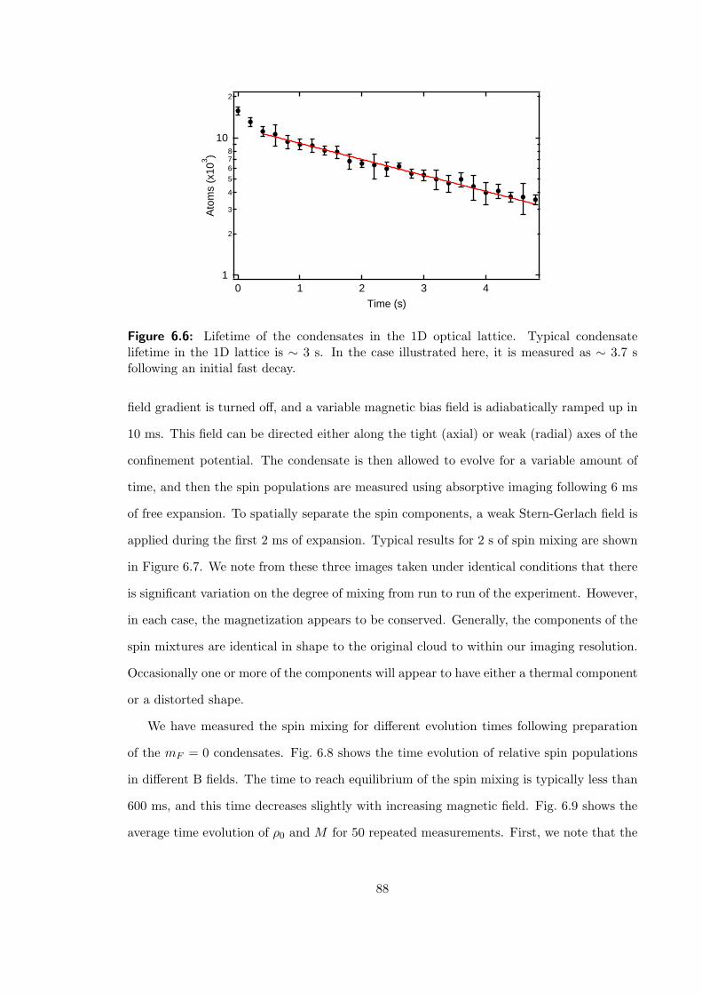
1

2

3

4

5

678

10

2

Ato

ms

(x10

3 )

43210

Time (s)

Figure 6.6: Lifetime of the condensates in the 1D optical lattice. Typical condensatelifetime in the 1D lattice is ∼ 3 s. In the case illustrated here, it is measured as ∼ 3.7 sfollowing an initial fast decay.

field gradient is turned off, and a variable magnetic bias field is adiabatically ramped up in

10 ms. This field can be directed either along the tight (axial) or weak (radial) axes of the

confinement potential. The condensate is then allowed to evolve for a variable amount of

time, and then the spin populations are measured using absorptive imaging following 6 ms

of free expansion. To spatially separate the spin components, a weak Stern-Gerlach field is

applied during the first 2 ms of expansion. Typical results for 2 s of spin mixing are shown

in Figure 6.7. We note from these three images taken under identical conditions that there

is significant variation on the degree of mixing from run to run of the experiment. However,

in each case, the magnetization appears to be conserved. Generally, the components of the

spin mixtures are identical in shape to the original cloud to within our imaging resolution.

Occasionally one or more of the components will appear to have either a thermal component

or a distorted shape.

We have measured the spin mixing for different evolution times following preparation

of the mF = 0 condensates. Fig. 6.8 shows the time evolution of relative spin populations

in different B fields. The time to reach equilibrium of the spin mixing is typically less than

600 ms, and this time decreases slightly with increasing magnetic field. Fig. 6.9 shows the

average time evolution of ρ0 and M for 50 repeated measurements. First, we note that the

88

mF 01 -1

Figure 6.7: Spin mixing of spinor condensates in the optical trap. The mixing processstarts with a pure mF = 0 condensate in the optical trap. Three separate measurements ofthe spin state are shown after 2 s of spin mixing.

magnetization, M , is conserved throughout the mixing to within a few percent. Although

the data does suggest a drift of M below zero by a small amount -3.5±2% (the uncertainty

here and error bars in the data are purely statistical), the deviation, if any, is compara-

ble to our uncertainties in measuring populations (∼3%), limited by the absorptive imaging

technique. Secondly, there is an almost ten fold reduction in the statistical noise of the mag-

netization relative to that of the total population, which varies 17% from shot to shot. This

suggests that the fluctuations of ρ1 and ρ−1, which are coupled from the mixing processes

in Eq. (6.1), are quantum correlated. These correlations underly theoretical predictions for

spin squeezing and entanglement in the system [132]. Thirdly, the relaxation of ρ0 to the

steady state value is not monotonic but instead shows a damped oscillation at 4 Hz. Such

oscillations are a natural outcome of coherent spinor mixing and will be discussed in greater

detail in Chapter 7.

The behavior of the mean-field ground state of spinors in magnetic fields can be under-

stood from the energy contour given by Eq. 5.28, E = cρ0

[(1− ρ0) +

√(1− ρ0)2 −M2 cos θ

]+

δ(1− ρ0). Here ρ0 is the fractional population of m0 state, M is the magnetization, and θ

is the spinor phase defined in the previous chapter. The energy contour of ferromagnetic

and anti-ferromagnetic spinors for M = 0 are shown Fig. 6.10. In zero magnetic field, the

ferromagnetic ground state is ρ0 = 1/2, θ = 0, and the anti-ferromagnetic ground state

θ = π, however, ρ0 is not uniquely determined in (0, 1) [137]. When the field is not zero,

the anti-ferromagnetic ground state reduced immediately to ρ0 = 1, while in the ferromag-

netic case, ρ0 will gradually increase as B field increases. This gives a clear signature for

distinguishing ferromagnetic and anti-ferromagnetic spinors.

89

1.0

0.5

0.0

3.02.01.00.0

B = 0.54 G

1.0

0.5

0.0

ρm

3.02.01.00.0Time (s)

B = 0.32 G1.0

0.5

0.0

3.02.01.00.0

B = 0.38 G

1.0

0.5

0.0

3.02.01.00.0

B = 0.49 G

1.0

0.5

0.0

3.02.01.00.0

B = 0.43 G

1.0

0.5

0.0

3.02.01.00.0

B = 0.59 G

Figure 6.8: Plots of the relative spin populations vs. time in different magnetic fields. HereRGB colors represent the relative population of mF = 1, 0,−1 states.

1.0

0.8

0.6

0.4

0.2

0.0

(nor

mal

ized

)

1.00.80.60.40.20.0

Time (sec)

ρ0

M

Figure 6.9: Plot of the fraction in the mF =0 state n0 and magnetization M (open circle)vs. time. In this measurement, M is determined to be 0.5±0.8% initially and -3.5±2% aftermixing. Note that there is a 8.5-fold reduction on the fluctuation of M compare to that ofthe total population (which is measured to be 17%). Clear population oscillations of n0 areseen, and the fluctuation in n0 is 6.6 fold of that of M . This data was taken at a bias fieldof 100 mG

90

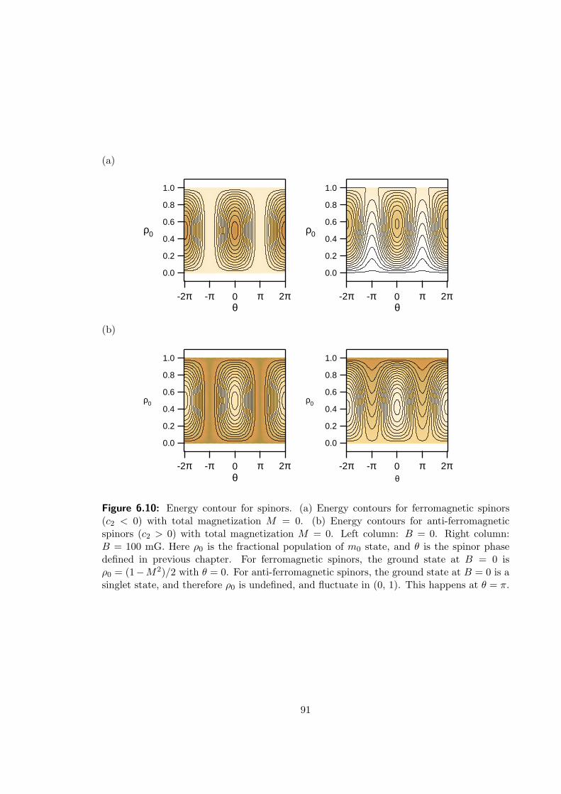
(a)

1.0

0.8

0.6

0.4

0.2

0.0

ρ0

θ

1.0

0.8

0.6

0.4

0.2

0.0

ρ0

θ0 2π-2π π-π 0 2π-2π π-π

(b)

1.0

0.8

0.6

0.4

0.2

0.0

ρ0

θ

1.0

0.8

0.6

0.4

0.2

0.0

ρ0

θ0 2π-2π π-π 0 2π-2π π-π

Figure 6.10: Energy contour for spinors. (a) Energy contours for ferromagnetic spinors(c2 < 0) with total magnetization M = 0. (b) Energy contours for anti-ferromagneticspinors (c2 > 0) with total magnetization M = 0. Left column: B = 0. Right column:B = 100 mG. Here ρ0 is the fractional population of m0 state, and θ is the spinor phasedefined in previous chapter. For ferromagnetic spinors, the ground state at B = 0 isρ0 = (1−M2)/2 with θ = 0. For anti-ferromagnetic spinors, the ground state at B = 0 is asinglet state, and therefore ρ0 is undefined, and fluctuate in (0, 1). This happens at θ = π.

91

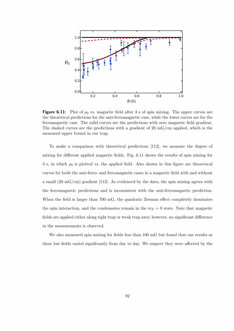
1.0

0.8

0.6

0.4

0.2

0.0

ρ0

1.00.80.60.40.2

B (G)

Figure 6.11: Plot of ρ0 vs. magnetic field after 3 s of spin mixing. The upper curves arethe theoretical predictions for the anti-ferromagnetic case, while the lower curves are for theferromagnetic case. The solid curves are the predictions with zero magnetic field gradient.The dashed curves are the predictions with a gradient of 20 mG/cm applied, which is themeasured upper bound in our trap.

To make a comparison with theoretical predictions [112], we measure the degree of

mixing for different applied magnetic fields. Fig. 6.11 shows the results of spin mixing for

3 s, in which ρ0 is plotted vs. the applied field. Also shown in this figure are theoretical

curves for both the anti-ferro- and ferromagnetic cases in a magnetic field with and without

a small (20 mG/cm) gradient [112]. As evidenced by the data, the spin mixing agrees with

the ferromagnetic predictions and is inconsistent with the anti-ferromagnetic prediction.

When the field is larger than 700 mG, the quadratic Zeeman effect completely dominates

the spin interaction, and the condensates remain in the mF = 0 state. Note that magnetic

fields are applied either along tight trap or weak trap axes; however, no significant difference

in the measurements is observed.

We also measured spin mixing for fields less than 100 mG but found that our results at

these low fields varied significantly from day to day. We suspect they were affected by the

92

stray AC magnetic fields present in the chamber 1. These fields are capable of driving off-

resonant rf-transitions between the Zeeman sub-levels. We observed this directly by creating

a F = 1,mF = −1 condensate (for which there is no spin mixing due to conservation of

magnetization) and measuring the final spin population. For magnetic fields greater than

100 mG, the magnetization remains conserved, while at lower fields, the mF = −1 atoms

are quickly pumped by the AC fields (within 100 ms for fields <10 mG) to other Zeeman

states. In addition, in low fields atoms could also undergo diabatic spin flips when the

Stern-Gerlach separation is performed at the end of each spinor experiment run.

Mean-field theory predicts that the spinor phase is θ = θ1 + θ−1 − 2θ0 = 0 for ferro-

magnetic ground state. We attempted to directly measure the phase relationship between

the spinor components [114] by performing an interference experiment between two spinor

condensates created in adjacent lattice sites. In the absence of dephasing mechanisms, we

would expect to see clear interference fringes in time-of-flight measurements both before and

after spin mixing. In the measurement shown in Fig. 6.12, clear interference fringes were

visible initially, while fringes were typically not observed after mixing. It is quite possible

however that the observed dephasing of the interference pattern was caused by small field

variations between two sites due to a stray magnetic field gradient (< 20 mG/cm) 2.

6.3 Observation of Spin-2 Dynamics

In the studies in previous sections, we have used microwave tuned to F = 1 and F = 2

transitions to measure the magnetic field. This microwave transition also allows to to study

F = 2 spinors. To do that, we coherently excite the pure F = 1,mF = 0 condensates to

F = 2,mF = 0 using microwave fields tuned to 6.8 GHz. Additionally, by controlling the

bias field, the microwave frequency, and the initial Zeeman state in the F = 1 manifold,

1Outside the chamber, magnetic field is monitored by a 3-axis fluxgate magnetometer. The AC magneticfield is measured to be 10− 15 mG, and they are mainly 60 Hz and 300 Hz noises from powered equipmentsnearby. Inside the chamber the B field is measured by microwave spectroscopy synchronized with 60 Hz linesignal, and we found the frequency shift at different phases of a 60 Hz cycle is equivalent to a AC field of≤ 5 mG

2To determine magnetic fields at the trap location, we employ microwave spectroscopy on the fieldsensitive F = 1 → F = 2 hyperfine transitions which is sensitive to within 2 mG. Furthermore, the fieldgradient is determined to be <20 mG/cm by measuring fields at different trap locations.

93

t = 0 s t = 1 s

mF 1 0 -1

Figure 6.12: Interference of two spinor condensates before and after spin mixing. At timezero, interference of two pure m0 condensates created in two adjacent lattice sites presentsclear interference fringe. After spin mixing for 1 s in a field of 100 mG, fringes are typicallynot observed.

we can pump the condensate to any Zeeman sub-level of the excited hyperfine manifold.

The |F = 2,m = 0〉 condensate is observed to decay as shown in Fig 6.13(a). Following

an initially rapid decay, it decays exponentially with a time constant of 250 ms. Despite

the short lifetime in the excited hyperfine manifold, we still observe spin mixing within 50

ms, and magnetization conservation is also observed during the mixing, as shown in Fig.

6.13(b).

In summary, we have observed spin mixing of 87Rb spinor condensates in F = 1 and F =

2 hyperfine manifolds in an optical trap. The observed equilibrium spinor configurations

of the lower manifold confirms that F = 1 87Rb is ferromagnetic. The magnetization

was conserved within the measurement errors during the entire spin mixing process. The

reduced noise of magnetization suggests quantum correlation of the spin dynamics, which

underlies spin squeezing and spin entanglement.

94

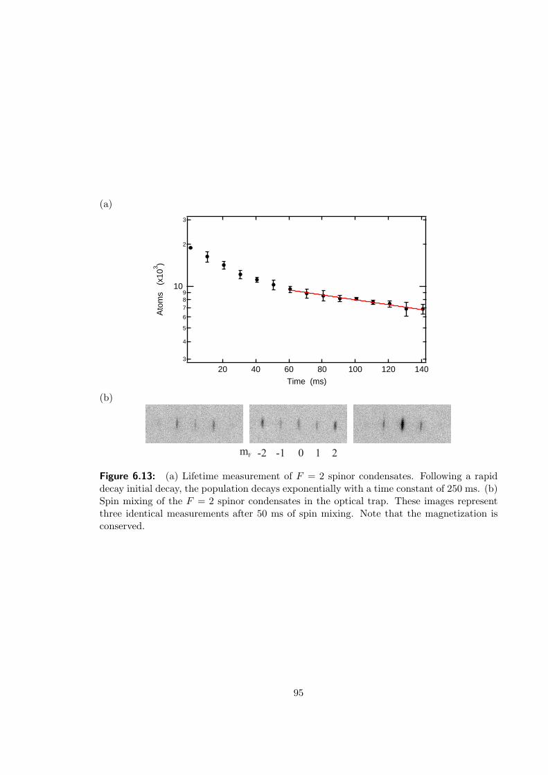
(a)

3

4

5

6

789

10

2

3

Ato

ms

(x1

03 )

14012010080604020

Time (ms)

(b)

-2 0-1 1 2mF

Figure 6.13: (a) Lifetime measurement of F = 2 spinor condensates. Following a rapiddecay initial decay, the population decays exponentially with a time constant of 250 ms. (b)Spin mixing of the F = 2 spinor condensates in the optical trap. These images representthree identical measurements after 50 ms of spin mixing. Note that the magnetization isconserved.

95

CHAPTER VII

COHERENT SPINOR DYNAMICS

In this chapter, we describe our observation of coherent spin-mixing collisions. Collisions in

a thermal gas are perceived as random or incoherent as a consequence of the large numbers

of initial and final quantum states accessible to the system. In a quantum gas, e.g. a Bose-

Einstein condensate or a degenerate Fermi gas, the phase space accessible to low energy

collisions is so restricted that collisions become coherent and reversible.

Collisional coherence is an important theme in quantum degenerate gases. For sin-

gle component condensates, such as spin-polarized atomic condensates confined in a mag-

netic trap, the coherence of the collisional interactions has been well-established in early

measurements of condensate mean-field energy [138] and correlations [18] as well as in

demonstrations of matter-wave interference [10] and superfluid behaviour [25, 26, 27]. Col-

lisional coherence in more complicated systems has led to remarkable results, including

reversible atom-molecule formation across a Feshbach resonance for both bosonic and fermi-

onic [139, 140] atoms, and coherent collisions in optical lattices [14, 12].

In this chapter we show that the collisional coherence extends to the internal spin de-

grees of freedom of a spin-1 Bose gas by observing coherent and reversible spin-changing

collisions in spin-1 condensates. In a spin-1 condensate, two atoms with spin states m1 and

m−1 can coherently and reversibly scatter into final states containing two atoms with spin

component m0 and vice-versa (Fig. 7.1a). Spin mixing has been observed in both F = 1 and

F = 2 condensates in the last chapter [42, 44, 45, 125]. Experiments so far have revealed

mostly incoherent relaxation of initially non-equilibrium spin populations to lower energy

configurations from which the sign of the spin interaction parameter c2 was determined.

Although strongly-damped oscillations in spin populations were observed in our initial ex-

periments discussed in Chapter 6 and by others [44, 125], their interpretations are limited

due to the fact that the initial spin configurations in these experiments were metastable,

96

and evolution from these states is noise-driven [42, 44, 45, 125]. Nonetheless, from these

observations, as well as studies of spin domain formation, it was possible to determine the

magnetic nature of the ground states.

7.1 Initiation of Coherent Spin Mixing

In the mean-field limit, condensates are described by coherent states, and coherent spin

mixing is simply a process of atomic four-wave mixing, which can be seen in Eq. (5.23). The

spin mixing rate is proportional to the product of the amplitudes of the order parameters,

and in most cases it requires presence of all three spin components. To better demonstrate

the coherent spin mixing, we start with a non-stationary spin configuration. Under the

single-mode approximation (SMA), the internal state of a coherent superposition of m0

and m−1 condensates can be expressed as ~ζ = (0, ζ0, ζ−1). With this initial condition, the

spin mixing rate at time zero is nonzero, and it is given by i~ ζ1 = c ζ20 ζ∗−1 according to

Eq. (5.25). Indeed, the m1 component is generated from a nonlinear wave mixing of the

other two components, which are macroscopically occupied at time zero, and it is this initial

configuration that deterministically initiates the spin mixing. If one starts with a pure m0

or a mixture of m1 and m−1 condensates, the initial mixing rate should be zero according

to Eq. (5.25), and it would take much longer time to build up the spin mixing rate. In these

cases, technical noise is more likely to play a role in the initiation of spin mixing. This can

explain the exceptionally large noise on the spin population oscillation amplitude presented

in Fig. 6.9.

To investigate the coherent dynamics of this system, we begin with 87Rb condensates

created in the single focus trap. The condensates created in this optical trap are generally in

a mixture of all F = 1 spin states and reveal complicated spatial domains. To create a well-

characterized initial condition, we apply a magnetic field gradient during the evaporative

cooling [45], which results in pure mF = −1 condensate containing 150,000 atoms. This

state is stable against both local and global spin dynamics due to the conservation of angular

momentum. The trap frequencies are 2π(190,170,17) rad/s, and the condensate density

and the Thomas-Fermi (T-F) radii are estimated to be 2.1×1014 cm−3 and (3.2,3.6,36) µm

97

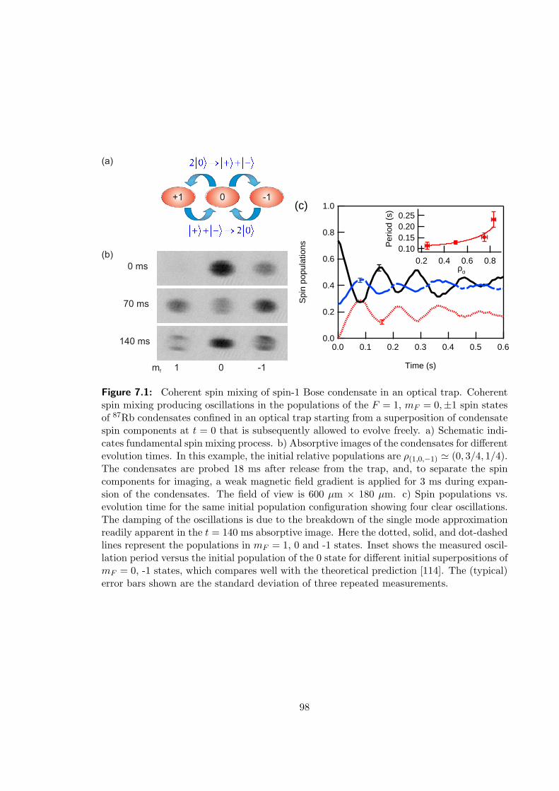
m 1 0 -1f

0 ms

70 ms

140 ms

+1 -10

(a)

(b)

1.0

0.8

0.6

0.4

0.2

0.0

Spi

n po

pula

tions

0.60.50.40.30.20.10.0

Time (s)

0.250.200.150.10P

erio

d (s

)

0.80.60.40.2ρο

(c)

Figure 7.1: Coherent spin mixing of spin-1 Bose condensate in an optical trap. Coherentspin mixing producing oscillations in the populations of the F = 1, mF = 0,±1 spin statesof 87Rb condensates confined in an optical trap starting from a superposition of condensatespin components at t = 0 that is subsequently allowed to evolve freely. a) Schematic indi-cates fundamental spin mixing process. b) Absorptive images of the condensates for differentevolution times. In this example, the initial relative populations are ρ(1,0,−1) ' (0, 3/4, 1/4).The condensates are probed 18 ms after release from the trap, and, to separate the spincomponents for imaging, a weak magnetic field gradient is applied for 3 ms during expan-sion of the condensates. The field of view is 600 µm × 180 µm. c) Spin populations vs.evolution time for the same initial population configuration showing four clear oscillations.The damping of the oscillations is due to the breakdown of the single mode approximationreadily apparent in the t = 140 ms absorptive image. Here the dotted, solid, and dot-dashedlines represent the populations in mF = 1, 0 and -1 states. Inset shows the measured oscil-lation period versus the initial population of the 0 state for different initial superpositions ofmF = 0, -1 states, which compares well with the theoretical prediction [114]. The (typical)error bars shown are the standard deviation of three repeated measurements.

98

respectively. The lifetime of the condensate is measured to be 3 s. Coherent spin state

superpositions are created from the pure mF = −1 condensates by applying a sequence

of phase-coherent microwave pulses tuned to F = 1 ↔ F = 2 transitions. The pulses are

applied at a field of 420 mG to separate out the transitions between the different Zeeman

sub-levels. Following the pulse sequence, the magnetic field is ramped from 420 mG to 15

mG in 10 ms. Typical pulse lengths are 20 µs for a F = 1 ↔ F = 2 pulse. Following this

state preparation, the condensate is allowed to freely evolve in the optical trap. A typical

evolution is shown in Fig. 7.1c for an initial spin configuration of ρ(1,0,−1) ' (0, 0.75, 0.25).

Up to four distinct oscillations are observed in this example before the spin populations

damp to a steady state. These oscillations demonstrate the coherence of the spin mixing

process.

The oscillations are observed to damp with a time constant of 250 ms, and the damping

coincides with the appearance of spatial spin structures apparent in the images in Fig. 7.1b.

These structures indicate the invalidation of the SMA underlying Eq. (5.23) and lead to a

complicated interplay of the internal and external dynamics that ultimately transfers the

internal spin energy into spatial domain structures [114]. Detailed studies of these domain

structures will be presented in the next chapter.

7.2 Measuring c2

We have measured the spin oscillation frequency for different initial spin populations. These

data are shown in the inset of Fig. 7.1c. and show good agreement with theoretical pre-

dictions, c√

1− ρ20 [114, 117] which can be derived from Eqs. (5.26-5.27). These measure-

ments provide a direct determination of the magnitude of the spin interaction energy [54],

|c|/~ = 2π × 4.3(3) rad/s for the case shown here. These oscillation frequencies at low

magnetic field do not determine the sign of c (c2), however it was established by studies of

the nature of the ground state in the last chapter [44, 45] that c2 < 0 for the F = 1 manifold

of 87Rb. As we shall see in Fig. 7.4, the negative sign of c2 is reconfirmed in the present

study. This value of c, combined with the measured condensate density, n = 2.1(4)× 1014

cm−3, determined from the rate of the condensate expansion during time-of-flight shown

99

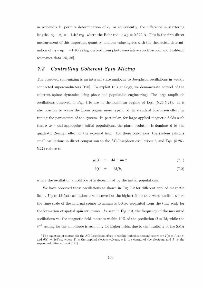
in Appendix F, permits determination of c2, or equivalently, the difference in scattering

lengths, a2 − a0 = −1.4(3)aB, where the Bohr radius aB = 0.529 A. This is the first direct

measurement of this important quantity, and our value agrees with the theoretical determi-

nation of a2− a0 = −1.40(22)aB derived from photoassociative spectroscopic and Feshbach

resonance data [55, 56].

7.3 Controlling Coherent Spin Mixing

The observed spin-mixing is an internal state analogue to Josephson oscillations in weakly

connected superconductors [128]. To exploit this analogy, we demonstrate control of the

coherent spinor dynamics using phase and population engineering. The large amplitude

oscillations observed in Fig. 7.1c are in the nonlinear regime of Eqs. (5.26-5.27). It is

also possible to access the linear regime more typical of the standard Josephson effect by

tuning the parameters of the system. In particular, for large applied magnetic fields such

that δ À c and appropriate initial populations, the phase evolution is dominated by the

quadratic Zeeman effect of the external field. For these conditions, the system exhibits

small oscillations in direct comparison to the AC-Josephson oscillations 1, and Eqs. (5.26 -

5.27) reduce to

ρ0(t) ' Aδ−1 sin θ, (7.1)

θ(t) ' −2δ/~, (7.2)

where the oscillation amplitude A is determined by the initial populations.

We have observed these oscillations as shown in Fig. 7.2 for different applied magnetic

fields. Up to 12 fast oscillations are observed at the highest fields that were studied, where

the time scale of the internal spinor dynamics is better separated from the time scale for

the formation of spatial spin structures. As seen in Fig. 7.3, the frequency of the measured

oscillations vs. the magnetic field matches within 10% of the prediction Ω = 2δ, while the

δ−1 scaling for the amplitude is seen only for higher fields, due to the invalidity of the SMA

1The equation of motion for the AC-Josephson effect in weakly-linked superconductors are I(t) = Ic sin θ,and θ(t) = 2eV/~, where V is the applied electric voltage, e is the charge of the electron, and Ic is thesuperconducting current [141].

100

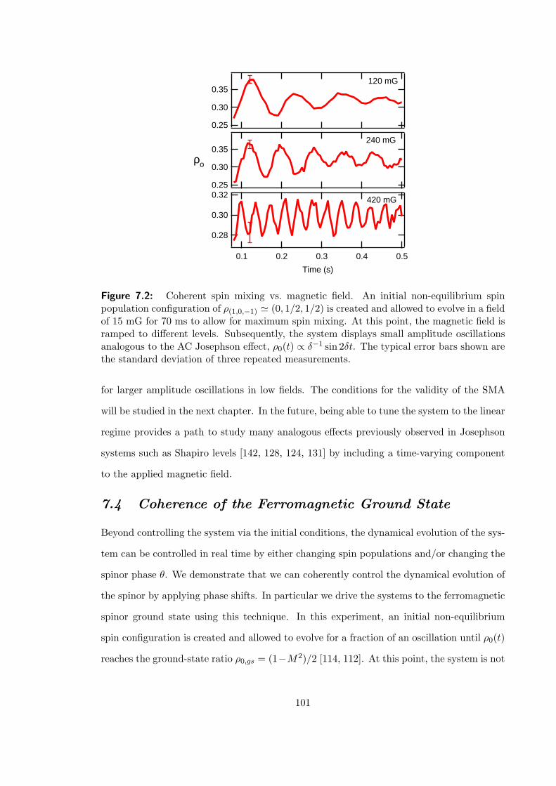
0.32

0.30

0.28

0.50.40.30.20.1

Time (s)

420 mG

0.35

0.30

0.25

120 mG

0.35

0.30

0.25

ρο

240 mG

Figure 7.2: Coherent spin mixing vs. magnetic field. An initial non-equilibrium spinpopulation configuration of ρ(1,0,−1) ' (0, 1/2, 1/2) is created and allowed to evolve in a fieldof 15 mG for 70 ms to allow for maximum spin mixing. At this point, the magnetic field isramped to different levels. Subsequently, the system displays small amplitude oscillationsanalogous to the AC Josephson effect, ρ0(t) ∝ δ−1 sin 2δt. The typical error bars shown arethe standard deviation of three repeated measurements.

for larger amplitude oscillations in low fields. The conditions for the validity of the SMA

will be studied in the next chapter. In the future, being able to tune the system to the linear

regime provides a path to study many analogous effects previously observed in Josephson

systems such as Shapiro levels [142, 128, 124, 131] by including a time-varying component

to the applied magnetic field.

7.4 Coherence of the Ferromagnetic Ground State

Beyond controlling the system via the initial conditions, the dynamical evolution of the sys-

tem can be controlled in real time by either changing spin populations and/or changing the

spinor phase θ. We demonstrate that we can coherently control the dynamical evolution of

the spinor by applying phase shifts. In particular we drive the systems to the ferromagnetic

spinor ground state using this technique. In this experiment, an initial non-equilibrium

spin configuration is created and allowed to evolve for a fraction of an oscillation until ρ0(t)

reaches the ground-state ratio ρ0,gs = (1−M2)/2 [114, 112]. At this point, the system is not

101

(a)

30

25

20

15

10

5

0

f (H

z)

0.40.30.20.10.0

B (G)

(b)

0.20

0.15

0.10

0.05

0.00

Am

plitu

de: ρ

0

0.40.30.20.10.0

B (G)

Figure 7.3: Spin mixing vs. B field. Solid curves are the theoretical predictions. The devia-tion between the theoretical prediction and the measurements on the oscillation amplitudesin low fields is due to that the internal spinor energy used to drive spin mixing are coupledout to spatial degrees of freedom to drive spatial dynamics.

102

in the ground state because θ 6= (θgs = 0) (and it is still oscillating!) At this moment, we

briefly pulse on a magnetic field of 0.6 G to apply a phase shift to the spinor, ∆θ =∫

δ(t)dt.

The evolution of the system is recorded in Fig. 7.4a for different pulse durations. We find

that for particular applied phase shifts, the spinor condensate is brought to its ground state,

evidenced by the subsequent lack of population oscillation. For other applied phase shifts,

the system is driven to different points in the phase space of the system, for which the

subsequent evolution of the system is dramatically different and exhibits oscillations.

It is possible to reconstruct the dynamical trajectories of the system using the measured

ρ0(t), along with the known applied phase shifts and the equations of motion, Eqs. (5.26-

5.27). Although the damping evident in the measurement is due to the spatial dynamics

coupled to the internal spin mixing dynamics, a phenomenological phase damping term

may be added to Eq. (5.27) to represent the spatial varying spin mixing rate which is

responsible for damping the population oscillation. The reconstructed trajectories show

qualitative agreement with the measurements in the time domain. The trajectories are

plotted on the phase space diagram of the system (Fig. 7.4b). Also shown in the figure

are the contours of equal energy of the spinor given by Eq. (5.28). The trajectories clearly

show that the system tends to damp to the minimum energy points (i.e. the ferromagnetic

spinor ground state), which is ρ0 ' 3/8, θgs = 0 mod (2π) for M = 1/2, c < 0 and δ ≈ 0.

For the case of anti-ferromagnetic interactions, such as in 23Na, c > 0, the energy contours

differ only in sign, and the system would instead relax to ρ0 = 1, θgs = π mod (2π) within

the validity of the SMA [114, 112].

To demonstrate explicitly the coherence of the spinor ground state, we impart a second

phase shift to the system at later times to displace the system to a different point in phase

space. As anticipated, the second phase shift is found to re-initiate the spin mixing dynamics

(Fig. 7.4c) when ∆θ 6= 0 mod (2π). We have used this technique to determine the ground

state spinor decoherence time by measuring the amplitude of the subsequent oscillations for

different delay times of the second pulse. The spinor decoherence time is found to be 3 s, and

is shown in Fig. 7.5. This decoherence time is approximately the lifetime of the condensate

and is much longer than the damping time (< 0.3 s) of spin population oscillations, which

103

0.5

0.4

0.3

0.2

ρο

0.5

0.4

0.3

0.2

ρο

0.5

0.4

0.3

0.2

0.1

0.0

ρο

−4π −3π −2π −π 0 πφ (rad)

0.50.0B

(G

)

0.60.40.20.0Time (s)

τ1 τ2

0.50.0B

(G

)

0.60.40.20.0Time (s)

τ1

(a)

(b)

(c)

Figure 7.4: Coherent control of spinor dynamics. a) An initial spin configuration ofρ(1,0,−1) ' (0, 1/2, 1/2) is allowed to evolve in a field of 15 mG for 14 ms at which pointthe populations reach the values corresponding to the ferromagnetic ground state at thismagnetization: ρ(1,0,−1) ' (1/16, 3/8, 9/16). Then, a pulse of 600 mG field is applied to shiftthe spinor phase. The dashed, solid and dotted curves represent pulse widths of τ1 = 20, 24.4and 30 ms respectively. For certain applied phase shifts, the coherent spin mixing can behalted. This occurs for τ1 = 24.4 ms corresponding to phase shift ∆θ = −2.5π and for τ1 =5.3 ms corresponding to ∆θ = −0.5π. b) Reconstructed dynamical trajectories of the systemdetermined by fitting the experiment data to Eq.(5.26-5.27) including a phenomenologicalphase damping term. The free parameters of the fit are the damping coefficient and theunknown (but reproducible) initial spinor phase resulting from the state preparation thatdepends on the applied microwave pulse width and the duration in the upper hyperfinemanifold. The contours show curves of equal energy. c) To investigate the spin coherenceof the ground state spinor created by the first pulse with τ1 = 24.4 ms, a second pulseis applied at 300 ms to reestablish the oscillations. The solid, dashed and dotted curvescorresponds to τ2 = 0, 10 and 20 ms respectively. The typical error bars shown are thestandard deviation of three repeated measurements.

104

2

4

68

0.01

2

4

68

0.1

2

Spi

n m

ixin

g am

plitu

de: ρ

0

6543210

Time (s)

1

2

4

6810

2

4

68100

Total atom

s (x103)

Figure 7.5: Decoherence time of the spinor condensates. The lifetime of the condensateis measured to be 3.8 ± 0.5 sec, while the decoherence time of the spinor is 2.9 ± 0.5 sec.Since the amplitude presents a fast decay initially, the first point is exclude from the fit.We suspect the initial fast decay on the spin mixing amplitude is due to partial spatialseparation of m1 and m−1 component which will be shown in Chapter 8.

is is in the time scale of the spatial dynamics (∼ c2n).

As noted, the damping of the spin oscillations coincides with the appearance of spin

wave-like spatial structures in the spinor wave function (see images in Fig. 7.1b). Hence it is

clear that the SMA is not strictly valid for our system. These waves derive their energy from

the internal (spin) degrees of freedom, and it is this energy transfer that ultimately damps

the spin mixing. On the other hand, if the spinor condensate is driven to its ferromagnetic

ground state, as shown in Fig. 7.4b, there is no internal (spin) energy available for the

motional degrees of freedom, and spatial spin structures cannot form. Indeed in this case,

the three spin components are observed to have the same spatial wave function and appear

to be miscible. The details of this study will be shown in Chapter 8

The observation of coherent spinor dynamics in a ferromagnetic spin-1 system described

here paves the way for a host of future explorations. These systems are predicted to manifest

complex quantum correlated states exhibiting entanglement and squeezing, and in general, it

will be very interesting to explore the regime of small atom number < 1000, where sub-shot

noise effects should become important [54]. Viewing the spin-mixing dynamics as a type

of internal Josephson effect, many future explorations and manipulations of the system can

105

be envisaged following along the path of superconducting weak-links. Finally, the coupling

of the internal dynamics to the spatial wave function can be avoided in future experiments

by either decreasing the condensate radii relative to the spin healing length ξs and/or

operating at high magnetic fields where the time scales for mixing and damping are better

separated. On the other hand, the coupling of the internal and external degrees of freedom

in this system provide a new system for exploring nonlinear atom optical phenomena such

as spatial-temporal dynamics of four-wave mixing [143].

Coherence spin-mixing have also been demonstrated in a Mott state of atoms on a lattice

[144]. Their experiment involves a system of many copies of two atoms in each lattice site.

On the other hand, our system involves a few hundred thousand atoms and the observed

coherence reflects the presence of macroscopic spinor fields. High field oscillations have also

been observed in an experiment in Hamburg [145].

106

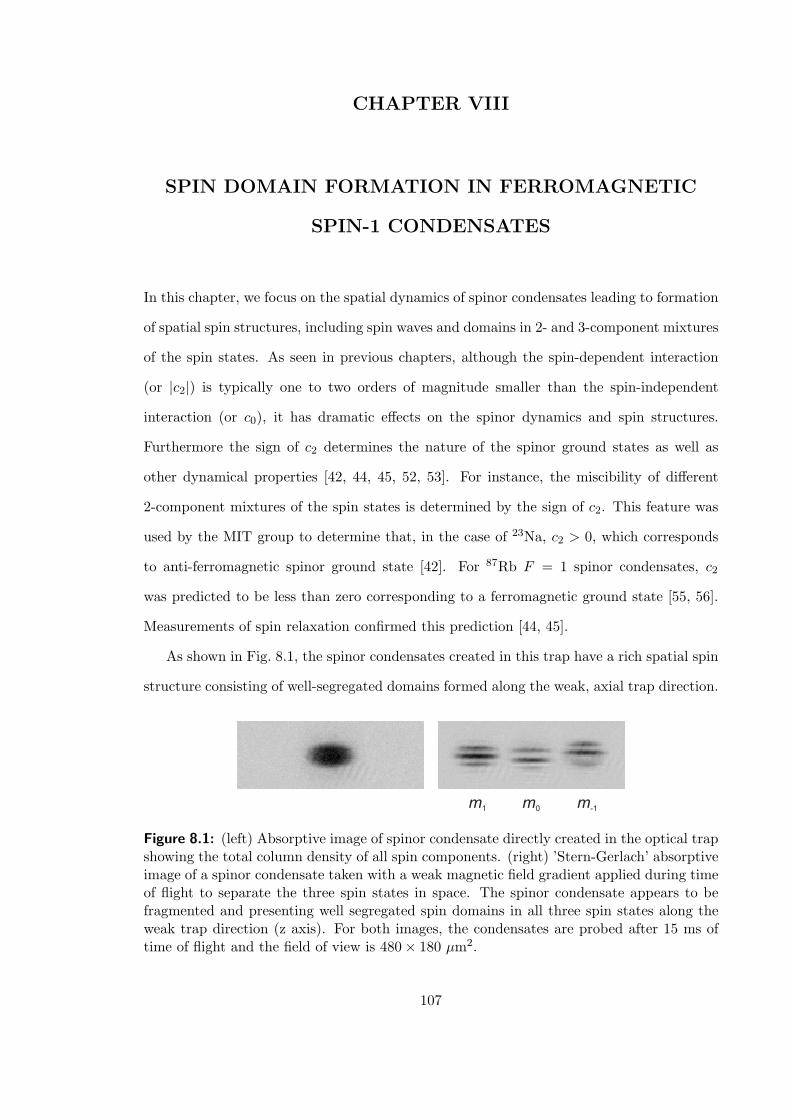
CHAPTER VIII

SPIN DOMAIN FORMATION IN FERROMAGNETIC

SPIN-1 CONDENSATES

In this chapter, we focus on the spatial dynamics of spinor condensates leading to formation

of spatial spin structures, including spin waves and domains in 2- and 3-component mixtures

of the spin states. As seen in previous chapters, although the spin-dependent interaction

(or |c2|) is typically one to two orders of magnitude smaller than the spin-independent

interaction (or c0), it has dramatic effects on the spinor dynamics and spin structures.

Furthermore the sign of c2 determines the nature of the spinor ground states as well as

other dynamical properties [42, 44, 45, 52, 53]. For instance, the miscibility of different

2-component mixtures of the spin states is determined by the sign of c2. This feature was

used by the MIT group to determine that, in the case of 23Na, c2 > 0, which corresponds

to anti-ferromagnetic spinor ground state [42]. For 87Rb F = 1 spinor condensates, c2

was predicted to be less than zero corresponding to a ferromagnetic ground state [55, 56].

Measurements of spin relaxation confirmed this prediction [44, 45].

As shown in Fig. 8.1, the spinor condensates created in this trap have a rich spatial spin

structure consisting of well-segregated domains formed along the weak, axial trap direction.

m0

m-1

m1

Figure 8.1: (left) Absorptive image of spinor condensate directly created in the optical trapshowing the total column density of all spin components. (right) ’Stern-Gerlach’ absorptiveimage of a spinor condensate taken with a weak magnetic field gradient applied during timeof flight to separate the three spin states in space. The spinor condensate appears to befragmented and presenting well segregated spin domains in all three spin states along theweak trap direction (z axis). For both images, the condensates are probed after 15 ms oftime of flight and the field of view is 480× 180 µm2.

107

On the other hand, the total density profile shows little structure and is well described

by the standard Thomas-Fermi wave function. The size of the observed spin domains

is 21 µm, which is comparable to the spin healing length, ξs ≈ 15 µm. The observed

spin domains appear to be created simultaneously with the formation of the 3-component

condensate. To study domain formation from a more controllable initial condition, we start

with preparing condensates all in the m−1 state developed in our previous experiment [45].

We then create 2-component condensates by using phase coherent microwave pulses tuned

to F = 1 ↔ F = 2 transitions and 3-component condensates via subsequent coherent spin

mixing following initial spin state preparation [146].

Recall the coupled Gross-Pitaevskii (GP) equations for the order parameters of a spin-1

condensate:

i~∂ψ±1

∂t= L±1ψ±1 + c2(n0 + n±1 − n∓1)ψ±1 + c2ψ

20ψ

∗±1 (8.1)

i~∂ψ0

∂t= L0ψ0 + c2(n1 + n−1)ψ0 + 2c2ψ

∗0ψ1ψ−1, (8.2)

where L±1,0 = −~2∇2/2m + Vt + E±1,0 + c0n. The terms Vt, E±1,0 and n±1,0 are the

trapping potential, Zeeman energies and densities for corresponding Zeeman projections

m±1,0, with the total density n = n1 +n0 +n−1. Two types of binary interactions presented

here are density and spin mean-field interactions, which are led by c0 and c2 coefficient

respectively. The second term in Eqs. 8.1-8.2, led by c2 coefficient, represents cross-phase

modulation (or particle exchange collisions), and it results in the (im)miscibility of different

Zeeman projections which can lead to phase separation and spin domain formation of two-

component superfluids. The last term in Eqs. 8.1-8.2 is responsible for coherent spin mixing

(or spin changing collisions) which causes spin populations to coherently interconvert among

different Zeeman states, and provides a path to relax to a lower energy spin configuration

in the presence of dissipation [42, 44, 45].

While the magnitude, |c2|n, determines the time scale of the spinor dynamics, the sign

of c2 determines the magnetic properties of the spinors and the dynamical stability of

spinor dynamics. Indeed, a spin-1 condensate offers a model system to study nonlinear

atom optics [146, 147, 148] — the external and internal dynamics are generally inseparable,

108

which provides a matter wave analogy of optical four-wave mixing in nonlinear media, and

is ideal for studying nonlinear, spatio-temporal dynamics. On the other hand, under certain

conditions the external and internal dynamics can be decoupled which greatly simplify the

dynamics and allows studies of different spinor dynamics in greater detail.

When the available spin interaction energy is insufficient to create spatial spin domains,

the external dynamics will be suppressed. This can occur when the spin healing length ξs

is larger than the dimension of the condensate, and ψ±1,0 share the same simple spatial

wave function, known as the single-mode approximation (SMA) [39, 40]. This leads to a

great simplification of Eq. 8.1-8.2. The internal dynamics are determined by ρ0(t), the

fractional population of the m0 state, and the spinor phase φ(t) ≡ φ1 + φ−1 − 2φ0, where

φi is the phase of the mi state. The populations of the other states are directly determined

by ρ±1 = (1 − ρ0 ±M)/2, where M = (N1 −N−1)/N is the normalized global magnetism

which is conserved, and Ni is the number of atoms in the mi state with N = N−1+N0+N1.

Within the SMA, the ground state spin populations and relative phase are readily found

for arbitrary magnetization and magnetic field by minimizing the single mode Hamiltonian,

E = cρ0

[(1− ρ0) +

√(1− ρ0)2 −M2 cos θ

]+ δ(1 − ρ0), [146, 114, 117]. In particular, for

c2 < 0, the energy of the system at low fields is minimized for spinor phase φ = 0 and

population ρ0 = (1−M2)/2. For other non-equilibrium populations or phases, the system

will have excess spin energy that can drive a coherent evolution of the spinor system.

The results in the previous chapter have shown that the magnitude and rate of the

coherent spin mixing can be tuned and even suppressed [146, 117]. In a field regime where

the external quadratic Zeeman effect δ overrides internal spinor interactions, or δ À |c2|n,

the system exhibits fast and small amplitude oscillations analogues to AC-Josephson oscil-

lations with ρ0(t) ∝ δ−1 sin 2δt [146]. Therefore, one can readily tune the amplitude of

spin mixing to arbitrarily small values by applying a high biased magnetic field. E.g., for

87Rb F = 1 condensate, if m1 component is removed and a field of > 500 mG is applied,

the amplitude of spin population oscillations can be reduced to < 1% of the total popula-

tion [146, 117]. This type of 2-component systems was used to determine the miscibility

of different spin components in anti-ferromagnetic Na spinor condensates [52]. The control

109

and separation of two different types of spinor dynamics in the last chapter and in this

chapter allow us to study the spatial spinor dynamics solely, or the interplay between these

dynamics and coherent spin mixing which naturally occurs in spin-1 condensates.

8.1 Miscibility of Spin Components

The miscibility of different spin components are simply determined by the system energy. If

the total system energy is lower when different components overlap compared to that when

they are spatially (phase) separated, then they are miscible; otherwise, they are immiscible.

The mean-field energy of the spinors can be obtained directly from the interaction Hamil-

tonian, Eq. 5.17. Recall that, in the mean-field limit, quantum fluctuations can be ignored

and the spinor field operators can be replaced with the ground state order parameters,

whose magnitudes are the square root of the densities, i.e.,

Ψi → ψi ∼ √ni, (8.3)

Ψ†i → ψ∗i ∼

√ni, (8.4)

where i = 1, 0,−1. Here Ψi, ψi, and ∼ √ni are the field operator, order parameter, and

the density of the ith spin component. Applying the above approximation to Eq. (5.17),

the mean-field energy is given by

EMF =12

∫d3rg1n

21 + g0n

20 + g−1n

2−1

+2g10n1n0 + 2g1−1n1n−1 + 2g0−1n0n−1

+4g1−1,00n0√

n1n−1, (8.5)

where g’s are the mean-field interaction coefficients. In particular, ga,b, gab, and g1−1,00

stand for the one-fluid (self), two-fluid (cross-state), and three-fluid interaction coefficients.

The values of g’s are listed in Table 5.1.

Eq. (8.5) can be readily applied to determine the miscibility of two-component conden-

sates. For a two-component condensate, it reduces to

E =12

∫(gan

2a + gbn

2b + 2gabnanb)d3r, (8.6)

110

If we assume equal population and homogeneous density for simplicity, the mean-field energy

for the case of overlapped condensate is simply given as

Eo =N2

2V(ga + gb + 2gab) , (8.7)

where N is the total number of atoms and V is the volume of the condensate. Similarly,

the total mean-field energy for the case of phase separation is given as

Es =N2

2

(ga

Va+

gb

Vb

), (8.8)

with the condition of equal pressure n2aga = n2

bgb at equilibrium. When Eo < Es or when

gab <√

gagb, two components are miscible; otherwise, they are immiscible [149, 123].

To study the miscibility of different spin components, we prepare two-component con-

densates with 75,000 atoms in each spin component [146] and allow them to evolve freely

in the optical trap before probing. To reduce the spin mixing amplitude the magnetic field

is kept > 420 mG, either along the tight (radial) or weak (axial) trap directions. When

the magnetic field is along the weak trap direction, the field gradient is also compensated

to < 0.2 mG/cm to minimize the phase separation caused by mechanical forces of the field

gradient. For 87Rb spin-1 spinors, the density mean-field, c0, and spin-spin mean-field, c2,

were estimated to be 7.79× 10−12 Hz·cm3 and −3.61× 10−14 Hz·cm3 respectively. The in-

teraction coefficients for intra- and inter- spin states are listed in Table 5.1, and their values

are found to be g±1,0 = g±1 = c0+c2 = 7.76×10−12 Hz·cm3, g0 = c0 = 7.79×10−12 Hz·cm3,

and g1,−1 = c0− c2 = 7.83× 10−12 Hz·cm3 [55, 56]. It is readily found that g0,±1 <√

g0g±1

and g1,−1 <√

g−1g1, therefore, m0 and m±1 states should be miscible and m1 and m−1

states should be immiscible. Our observations in Fig. 8.2 confirm those predictions and are

consistent with the previous observations of ferromagnetic behaviors of F = 1 87Rb spinors

[44, 45, 146]. We also notice that miscible condensates can still form domains when the

large condensates are agitated.

While the miscibility of a 2-component system is determined by the intra- and cross-

component mean-field interactions, number of spin domains formed, however, is determined

by the total spin (internal) energy accessible to the spatial (external) degrees of freedom

of the condensates. In a spin-1/2 condensate, spin mixing does not occur, and particle

111

m1

m0

m-1

Figure 8.2: Stern-Gerlach absorptive images of 2-component condensates that are allowedto evolve for 500 ms in a field of 420 mG. Domain formation in the lower frame indicatesthe immiscibility of the m±1 states while the lack of domains in the other frames indicatesthe miscibility of m0 and the other two states.

exchange collisions, which correspond to the two-fluid mean-field interactions, are solely

responsible for the spinor dynamics. Under the presence of dissipation, relaxation to the

ground state should lead two immiscible components to complete spatial (phase) separation.

The formation of interlaced domains such as in Fig. 8.1 and 8.2 indicates incomplete relax-

ation, and the released internal spin energy is stored as the quantum pressure or the kinetic

energy of the spinor condensates, which is revealed as complicated spinor order parameters

or meta-stable spatial domains [52].

8.2 Spin Wave and Domain Formation in FerromagneticCondensates

In a spin-1 system, the spinor mean-field energy not only causes spin domain formation,

but also can drive coherent spin mixing as shown in Chapter 7. When the condensate’s

dimension is larger than its spin healing length, the spin mixing dynamics are unstable

[150] and perturbations can cause irreversibly conversion of the internal spin energy to ex-

ternal kinetic energy, forming meta-stable domains. This mechanism leads to the invalidity

of the SMA. To demonstrate that spatial domains are induced by dynamical instability

112

of spin mixing, we initiate coherent spin mixing with initial fractional spin populations

(0, 0.75, 0.25) and allow condensates to evolve freely until the amplitude of population os-

cillations are damped out. Fig. 8.3.a and 8.3.b show both the theoretical and experiment

studies of the spatial-temporal dynamics of all three spin components along the weak trap

direction. In the theoretical modelling, small amplitude noises at level of 10−5 are added

to the order parameters of all three components at time zero [150, 151]. Our simulation

shows that spin mixing causes non-stationary spatial variation in each spin component.

This spatial variation presents a spin wave and persists for few seconds until the small noise

is amplified to a level where the symmetry of this pattern is broken [150]. Experimental

observations shown in Fig. 8.3.b verifies this type of spin waves; however, they only revive

during the first 3 mixing cycles which indicates much larger noise, and this quickly leads to

localization of wave fronts which serves to damp the spin mixing. Once the spin mixing is

mostly damped out each fragment is settled to a spin domain.

To demonstrate that energy stored in the 3-component spin domains is derived from the

internal energy used to drive spin mixing, and to identify the miscibility of 3-component

condensate in the ground state, we perform the following experiment. We create a conden-

sate with non-equilibrium spin population (0, 1/2, 1/2) and allow the coherent spin mixing

to take place in a low field. After mixing for 50 ms in which the spin populations reaches the

ground state configuration, (1/16, 3/8, 9/16), we impart a phase shift to bring the spinor

condensate to its ferromagnetic ground state as demonstrated in Chapter 7 [146]. Fig. 8.4.a

shows that all three components appear to be miscible and remain single domain there-

after. This indicates that domains will not form without excess kinetic energy, even when

the condensate dimension is larger than the spin healing length. On the other hand, since

the ground state should be a single-domain, it suggests that the formation of multiple do-

mains indicates incomplete relaxation of the internal spin mean-field energy [52]. We notice

in Fig. 8.4.b that although all three components appear to be miscible in the ferromag-

netic ground state, m±1 components still tend to avoid each other. However, since the m1

component is much smaller than the m−1 component, they are in weak-segregation phase

and are inter-penetrated [149]. At 0.3 s we impart a second phase shift to move the spinor

113

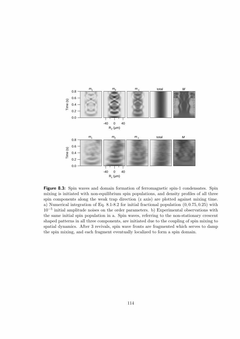
-40 0 40RZ (µm)

0.8

0.6

0.4

0.2

0.0

Tim

e (s

)

m1 m0 m-1 total M

-40 0 40Rz (µm)

0.8

0.6

0.4

0.2

0.0

Tim

e (s

)

m1 m0 m-1 total M

Figure 8.3: Spin waves and domain formation of ferromagnetic spin-1 condensates. Spinmixing is initiated with non-equilibrium spin populations, and density profiles of all threespin components along the weak trap direction (z axis) are plotted against mixing time.a) Numerical integration of Eq. 8.1-8.2 for initial fractional population (0, 0.75, 0.25) with10−5 initial amplitude noises on the order parameters. b) Experimental observations withthe same initial spin population in a. Spin waves, referring to the non-stationary crescentshaped patterns in all three components, are initiated due to the coupling of spin mixing tospatial dynamics. After 3 revivals, spin wave fronts are fragmented which serves to dampthe spin mixing, and each fragment eventually localized to form a spin domain.

114

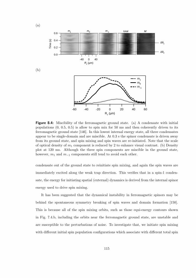
(a)

0.6

0.4

0.2

0.0

Tim

e (s

)

-40 0 40Rz (µm)

m1 m0 m-1 total M

∆θ1

∆θ2

(b)

-60 -40 -20 0 20 40 60Rz (µm)

m1

m0

m-1

Figure 8.4: Miscibility of the ferromagnetic ground state. (a) A condensate with initialpopulations (0, 0.5, 0.5) is allow to spin mix for 50 ms and then coherently driven to itsferromagnetic ground state [146]. In this lowest internal energy state, all three condensatesappear to be single-domain and are miscible. At 0.3 s the spinor condensate is driven awayfrom its ground state, and spin mixing and spin waves are re-initiated. Note that the scaleof optical density of m1 component is reduced by 2 to enhance visual contrast. (b) Densityplot at 120 ms. Although the three spin components are miscible in the ground state,however, m1 and m−1 components still tend to avoid each other.

condensate out of the ground state to reinitiate spin mixing, and again the spin waves are

immediately excited along the weak trap direction. This verifies that in a spin-1 conden-

sate, the energy for initiating spatial (external) dynamics is derived from the internal spinor

energy used to drive spin mixing.

It has been suggested that the dynamical instability in ferromagnetic spinors may be

behind the spontaneous symmetry breaking of spin waves and domain formation [150].

This is because all of the spin mixing orbits, such as those equi-energy contours shown

in Fig. 7.4.b, including the orbits near the ferromagnetic ground state, are unstable and

are susceptible to the perturbations of noise. To investigate that, we initiate spin mixing

with different initial spin population configurations which associate with different total spin

115

energy. Here we illustrate the spin mixing with initial spin configurations of (0, 0.5, 0.5),

and (0, 0.83, 0.17), and the experimental data are displayed in Fig. 8.5. The (0, 0.5, 0.5)

configuration is closer to the ferromagnetic ground state, and possesses less spinor energy

for driving the spin mixing. The second configuration is farther away from the ground state.

As shown in Fig. 8.5.a, spin mixing and spin waves revive for 5 mixing cycles before three

components phase separate, which is longer than in the case of Fig. 8.3.b. In contrast, spin

mixing and spin waves do not revive as seen in Fig. 8.5.b. These measurements suggest

that the degree of instability depends on the initial spinor energy; system with higher initial

spinor energy is more unstable. These measurements suggest that dynamical instability

indeed plays a role in domain formation.

Note that in the configuration shown in Fig. 8.5.b, it is observed in that m0 component

occupies the trap center at the onset of symmetry breaking, and the m1 component is

repealed to the edge of the trap. This is due to that m0 state is the largest component, and

m1 component is the smallest one [R]. The magnetic field gradient, similar to other noises,

may provide a small initial seed for unstable spinor modes, however, it is unlikely to be

responsible for the separation of spin components and domain formation as can be seen in

Fig. 8.5.b. In addition, release of higher internal spinor energy in the last case also leads to

more complicated spatial spin domains. This test provides the evidence that the dynamical

instability plays an important role in spontaneous domain formation.

8.3 Study of The Validity of Single-Mode Approximation

In the previous sections, the single focused trap has allowed us to study the 1D spatial

dynamics on a cigar shaped condensate in the trap, for the condensate size is larger than

the spin healing length along the axial direction. Is is of interest to compare the spin mixing

with and without the interplay with spatial dynamics. Fig. 8.6 lists three trap geometries

and the typical condensate size in these traps. For a typical density of 1014 cm−3, the spin

healing length in 87Rb is 10 - 15 µm. Therefore, the condensate size in the isotropic (cross)

trap and disk trap (lattice) is smaller than the spin healing length, and SMA may apply.

To investigate that, we perform spin mixing in a condensate created in an isotropic (cross)

116

(a)

-40 0 40Rz (µm)

0.8

0.6

0.4

0.2

0.0

Tim

e (s

)

m1 m0 m-1 total M

(a)

-40 0 40Rz (µm)

0.8

0.6

0.4

0.2

0.0

Tim

e (s

)

m1 m0 m-1 total M

Figure 8.5: Dynamical instability of spin mixing. a) Spin mixing is initiated in a condensatewith spin configuration of (0, 0.5, 0.5). It is observed that spin waves are revived for 5 mixingcycles before phase separation of spin components. b) For a spin configuration of (0, 0.83,0.17), spin waves do not revive, and domains form much quicker than in the case of a.

117

Cross trap 1-D lattice Single focus

~ spherical disk cigar

(2 ,2 ) ~ (7,7) mR Rr z m ( 2 ) ~ (8,1) mRz m2 ,R

r( ,2 ) ~ (7,70) mRz m2R

r

Figure 8.6: Trap geometry comparison. Condensates created in the cross trap and 1Dlattice have smaller condensate size than the spin healing length.

optical trap. The condensate contains 48,000 atoms, and the trap frequency is 2π × 230

rad/s. In this case the spin healing length is 11 µm while the condensate diameter is

only 7 µm. We observe 12 clear spin population oscillations, during which no spin waves

(crescent shaped patterns) and domain are formed in the two directions shown in our images.

The joint density plot along the axial direction are shown in Fig. 8.7.a, and plots of spin

population oscillation vs. time for the condensates in the cross trap and in the single focus

trap are displayed in Fig. 8.7.b. In the second plot, the coherent spin population oscillation

in the cross trap damps out with a time constant of 3 sec, while the damping time constant

is < 250 ms in the single focus trap. Our observations suggests that the SMA remains

valid when the condensate dimension is less than the spin healing length. When the SMA

is valid, the spinor energy is kept in the internal degrees of freedom which leads to larger

oscillation amplitude for longer time.

In summary, we have studied the miscibility and spin domain formation dynamics of

a ferromagnetic spin-1 condensate, and we show that spin domain formation is induced

by the spatial or spatio-temporal dynamics. We also show that in a spin-1 condensate,

the kinetic energy stored in multi-domains is derived from internal spin energy. When this

energy is not accessible or the condensate dimension is smaller its spin healing length, which

characterizes the smallest stable domain, different spin components appear to be miscible

and remain single domain. The implication of our observations and in this chapter and

the last chapter therefore points to the validity of the coupled Gross-Pitaevskii equations

used to describe spinor condensates, and verify that this spin-1 condensate is essentially the

118

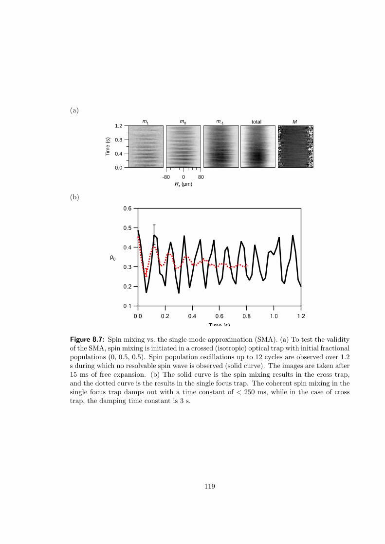
(a)

-80 0 80Rz (µm)

1.2

0.8

0.4

0.0

Tim

e (s

)

m1 m0 m-1 total M

(b)

0.6

0.5

0.4

0.3

0.2

0.1

ρ0

1.21.00.80.60.40.20.0

Time (s)

Figure 8.7: Spin mixing vs. the single-mode approximation (SMA). (a) To test the validityof the SMA, spin mixing is initiated in a crossed (isotropic) optical trap with initial fractionalpopulations (0, 0.5, 0.5). Spin population oscillations up to 12 cycles are observed over 1.2s during which no resolvable spin wave is observed (solid curve). The images are taken after15 ms of free expansion. (b) The solid curve is the spin mixing results in the cross trap,and the dotted curve is the results in the single focus trap. The coherent spin mixing in thesingle focus trap damps out with a time constant of < 250 ms, while in the case of crosstrap, the damping time constant is 3 s.

119

atomic matter wave analogue of optical four-wave mixing in nonlinear optical media [147].

This system thus provides a model for future studies on nonlinear dynamics, such as spinor

solitons and quantum chaos.

120

CHAPTER IX

FINAL REMARKS

In this thesis, we have described how we have successfully extended our all-optical BEC

technique to two new optical trap geometries. We can routinely create Bose-Einstein con-

densates by directly loading from a MOT with all three optical geometries. These three

geometries have proven to play important roles in the studies of spinor condensates. While

earlier experiments on spin-1 condensates were done with anti-ferromagnetic Na [42, 53, 52],

our studies on the ferromagnetic 87Rb spin-1 condensates have provided the other half of

the physical picture for spin-1 spinor condensates.

We have observed spin mixing dynamics in 87Rb F = 1 spinors and also in the excited

F = 2 spinors, from which we confirmed the predicted ferromagnetic nature of 87Rb ground

(F = 1) state. In the second spinor experiment, we have unambiguously observed the

coherent spin mixing by engineering the initial spin population and spinor phase, and from

which we determined the spin-dependent interaction strength. We have also demonstrated

coherent control of spin mixing, in which we drove the spinor condensate to and away from

its ferromagnetic ground state. Using this method, we have measured the decoherence time

of the ferromagnetic ground state.

The single focus trap geometry has allowed us to study spin domain formation and

spatio-temporal dynamics of spinor condensates. Our studies on coherent spin mixing and

spatial spinor dynamics thus validate the coupled Gross-Pitaevskii equations used to de-

scribe spin-1 condensates. This system is an atomic analogue to four-wave mixing of a laser

beam in Kerr media [147]. In the future this spin-1 condensate system will provide a model

system for studying atomic four-wave mixing and atom optics.

Coherent spin mixing is a type of internal Josephson oscillator, and therefore one can

expect to observe phenomena related to the Josephson effects in weak-linked superconduc-

tors, such as dynamical localization or the so-called Shapiro effects [142, 128, 124, 131].

121

In order to observe this effect, stable and persistent spin population oscillations are re-

quired. To achieve that, the single-mode approximation needs to be satisfied. We have

demonstrated that the cross trap geometry can forbid excitation of spatial spin waves and

continue spin mixing for longer time. The spin mixing frequency is proportional to the

condensate density, therefore reducing condensate density fluctuations should allow more

stable spin mixing rate. Alternatively, spin mixing in a high magnetic field should bring

the spin mixing to a regime where the external quadratic Zeeman effect dominates internal

spin interactions. In this regime, spin mixing will be independent of the condensate den-

sity. The downside, however, is that the spin mixing amplitude is small in a high field and

fluctuations of population from shot to shot will eventually limit the observation of spin

mixing. In the future, creating condensates in the cross trap with fewer fluctuations in total

population and density will be the key to increasing the number of oscillations.

Currently, our studies on spinor dynamics are in the mean-field limit regime where

quantum fluctuations are small and thus are neglected, and the spinor dynamics is well-

described by the Gross-Pitaevskii equation. When the condensate size contains only one

thousand atoms or less, quantum fluctuations become prominent and cannot be neglected

[54, 113]. This should allow us to study quantum spin mixing, or the so-called quantum

atom optics. In particular, this spin-1 system has been predicted to possess complex ground

states, spin squeezing, and spin entanglement via quantum spin mixing [54, 120, 132]. We

have previously observed reduced noise on magnetization, in the future, developing new

imaging techniques which is capable of shot-noise limit detection on only few hundred

atoms should allow us to study spin squeezing directly.

122

APPENDIX A

TABLE OF CONSTANTS AND PROPERTIES OF 87RB

Table A.1: Fundamental constants (2002 CODATA recommended values) and useful 87Rbproperties [57].

Quantity Symbol ValueFundamental Constants

Speed of Light c 2.997 924 58 ×108 m/s (exact)Permeability of Vacuum µ0 4π × 10−7 N/A2 (exact)Permittivity of Vacuum ε0 (µ0c

2)−1

Planck Constant h 6.626 069 3(11)×10−34 J sElementary Charge e 1.602 176 53(14)×10−19 C

Bohr Magneton µB 9.274 009 49(80)×10−24 J/TBohr Radius a0 0.529 177 208 3(19)×10−10 m

Bolzman Constant kB 1.380 650 3(24)×10−23 J/KBasic Properties of 87Rb

Atomic Number Z 37Atomic Mass m 1.44316060(11)× 10−25 kg

Natural Abundance 27.83%Nuclear Spin I 3/2

Ground (52S1/2) State PropertiesFine structure Lande g-factor gJ 2.002 319 304 373 7(80)

Nuclear g-factor gI -0.000995 141 4(10)Hyperfine Splitting νhf 6,834,682,610.90434(3) Hz

D2 (52S1/2 → 52P3/2) TransitionWavelength (vacuum) λ 780.241 209 686(13) nm

Lifetime τ 26.24(4) nsDecay Rate Γ 2π·6.065(9) MHz

|F = 2,mF = ±2〉 → |F ′ = 3,mF = ±3〉Saturation Intensity Isat 1.669(2) mW/cm2

Resonance Cross Section σ0 2.907×10−9 cm2

Scattering Lengths (s-wave)scattering length for spin-0 channel aF=0 101.8(2) a0

scattering length for spin-2 channel aF=2 100.4(1) a0

123

APPENDIX B

SPINOR DEGREES OF FREEDOM OF TWO SPIN-F

ATOMS UNDER COLLISION

Let N = 2f + 1, which represents the number of internal (Zeeman) states of a spin-f

particle. Then for two spin-f particles, the possible input channels are N2. However,

exchange symmetry (gij,kl = gji,kl) leads to only N2 − CN2 = N2 − N(N−1)

2! = N(N+1)2

input channels. By the same token, for each input channel, there are N(N+1)2 (≡ z) possible

output channels, without considering spin conservation. For the first input channel (if we

label those channels), there are z possible output channels. However, for the second input

channel, there are only z−1 output channels, since it contains a time-reversal (gij,kl = gkl,ij)

of one of the cases already counted in the first input channel. So, the total free parameters

are

ν = z2 − [1 + 2 + · · ·+ (z − 1)]

= z2 − 12z(z − 1)

= [N(N + 1)

2]2 − 1

2[N(N + 1)

2][N(N + 1)

2− 1]

=12[N(N + 1)

2]2 +

12[N(N + 1)

2]

=12

N(N + 1)2

[N(N + 1)

2+ 1]

=18(N2 + N)(N2 + N + 2). (B.1)

In the case of two spin-1 particles (F = 1), there are 6 input channels under exchange

symmetry, say, (1, 1), (1, 0), (1,−1), (0, 0), (0,−1),and (−1,−1). And for each input channel,

we have:

(1, 1) → (1, 1), (1, 0), (1,−1), (0, 0), (0,−1), (−1,−1):6 output channels under exchange

symmetry condition.

124

(1, 0) → (1, 0), (1,−1), (0, 0), (0,−1), (−1,−1): 5 output channels, we exclude the output

channel (1, 1), since (1, 0) → (1, 1) is the time-reversal of (1, 1) → (1, 0).

(1,−1) → (1,−1), (0, 0), (0,−1), (−1,−1): 4 output channels.

· · ·Therefore, there are only 6+5+4+3+2+1 = 21 free parameters need to be considered.

By using Eq. (B.1), we have N = 3 and ν = 18(32 + 3)(32 + 3 + 2) = 21, which agrees

with the above calculations.

125

APPENDIX C

SPIN COUPLING OF TWO SPIN-1 ATOMS

In a system of two coupled spin-1 bosons, the maximally aligned spin state is |F = 2, mF =

2〉 = |f = 1, mf = 1〉|f = 1,mf = 1〉. For convenient, here we define |F, M〉 = χFM , and

|f1 = 1, m〉 = χ(1)m and |f2 = 1,m〉 = χ

(2)m .

We can render the other M states using ladder operators:

F±|F, M〉 = ~√

F (F + 1)−M(M ± 1)|F, M ± 1〉.

Here F± is the rising/lowering operator for total spin. It can be expressed as the sum of

two operators for two atoms,

F± = f(1)± + f

(2)± ,

where f(1,2)± are the rising/lowering operators for atoms 1,2. Therefore,

F−χ22 = (f (1)

− + f(2)− )(χ(1)

1 χ(2)1 )

= ~√

2(χ(1)0 χ

(2)1 + χ

(1)1 χ

(2)0 )

= 2~ 1√2(χ(1)

0 χ(2)1 + χ

(1)1 χ

(2)0 )

= 2~χ21,.

By comparison, we find χ21 = 1√

2(χ(1)

0 χ(2)1 + χ

(1)1 χ

(2)0 ). Similarly, χ2

0 = 1√6(2χ

(1)0 χ

(2)0 +

χ(1)−1χ

(2)1 + χ

(1)1 χ

(2)−1), χ2

−1 = 1√2(χ(1)−1χ

(2)0 + χ

(1)0 χ

(2)−1), and χ2

−2 = χ(1)−1χ

(2)−1.

Since χ11 must be orthogonal to χ2

1, it is straightforward to show that χ11 = 1√

2(χ(1)

1 χ(2)0 −

χ(1)0 χ

(2)1 ). Applying the lowering operator to this state, we can further find χ1

0 = 1√2(χ(1)

1 χ(2)−1−

χ(1)−1χ

(2)1 ), and χ1

−1 = 1√2(χ(1)

0 χ(2)−1 − χ

(1)−1χ

(2)0 ).

Finally, since χ00 must be orthogonal to χ2

0 and χ10, and given that F±χ0

0 = 0, it can be

shown that χ00 = 1√

3(χ(1)

0 χ(2)0 − χ

(1)1 χ

(2)−1 − χ

(1)−1χ

(2)1 ).

By observation, we find that the states in the F = 0, 2 (F = 1) manifold are exchange

126

symmetric (anti-symmetric). Therefore, when the total external wavefunction of two col-

liding atoms are symmetric, the allowed total spin channels are F = even for bosons and

F = odd for fermions.

127

APPENDIX D

INTERACTION HAMILTONIAN OF SPIN-1 BOSE GAS

Recall Eq. 5.16:

Hint =12

∫d3~rc0Ψ

†iΨ

†jΨjΨi + c2Ψ

†iΨ

†j(~fjk ·~fil)ΨkΨl. (D.1)

The spin independent (c0) term in Eq. D.1 is given by

c0

2Ψ†

iΨ†jΨjΨi (D.2)

=c0

2[Ψ†

1Ψ†1Ψ1Ψ1 + Ψ†

0Ψ†0Ψ0Ψ0 +

Ψ†−1Ψ

†−1Ψ−1Ψ−1 + 2Ψ†

1Ψ†0Ψ0Ψ1 +

2Ψ†1Ψ

†−1Ψ−1Ψ1 + 2Ψ†

0Ψ†−1Ψ−1Ψ0].

The spin dependent (c2) terms are given by

c2Ψ†iΨ

†j(~fjk ·~fil)ΨkΨl =

c2

2Ψ†

iΨ†j(fx)ik(fx)jl + (fy)ik(fy)jl + (fz)ik(fz)jlΨkΨl,

where (fα)ik is the matrix element of the traceless Pauli spin-1 matrices, with α = x, y, z

and i, k = 1, 0,−1. Given the spin-1 matrices,

fx =1√2

0 1 0

1 0 1

0 1 0

, fy =i√2

0 −1 0

1 0 −1

0 1 0

, fz =

1 0 0

0 0 0

0 0 −1

,

We find

f (1)x f (2)

x = [(fx)10 + (fx)01 + (fx)0−1 + (fx)−10]2, (D.3a)

f (1)y f (2)

y = [(fy)10 + (fy)01 + (fy)0−1 + (fy)−10]2

= −[(fx)01 + (fx)−10]− [(fx)10 + (fx)0−1]2, (D.3b)

f (1)z f (2)

z = [(fz)11 + (fz)−1−1]2

= (fz)211 + (fz)2−1−1 + [(fz)11(fz)−1−1 + h.c.]. (D.3c)

128

Combining Eq. (D.3a) and (D.3b), we have

f (1)x f (2)

x + f (1)y f (2)

y

= [(fx)10 + (fx)01 + (fx)0−1 + (fx)−10]2 − [−(fx)10 + (fx)01 − (fx)0−1 + (fx)−10]2

= 2[(fx)01(fx)10 + (fx)−10(fx)10 + (fx)01(fx)0−1 + (fx)−10(fx)0−1] + h.c. (D.4)

Substitute Eq. (D.4) back into ( D.1), we find

c2

2(Ψ†

iΨ†j [(fx)ik(fx)jl + (fy)ik(fy)jl]ΨkΨl)

=c2

22[Ψ†

1Ψ†0Ψ0Ψ1 + Ψ†

1Ψ†−1Ψ0Ψ0 + Ψ†

0Ψ†0Ψ−1Ψ1 + Ψ†

0Ψ†−1Ψ−1Ψ0] (D.5)

Similarly, substituting Eq. (D.3c) back into (D.1), we have

c2

2(Ψ†

iΨ†j(fz)ik(fz)jlΨkΨl)

=c2

2[Ψ†

1Ψ†1Ψ1Ψ1 − 2Ψ†

1Ψ†−1Ψ−1Ψ1 + Ψ†

−1Ψ†−1Ψ−1Ψ−1] (D.6)

Combine eqn.(D.2), eqn.(D.6), and eqn.(D.5), we arrive at the interacting Hamiltonian,

Hint =12

∫d3~rc0(Ψ

†iΨ

†jΨjΨi) + c2(Ψ

†iΨ

†j [(fm)ik(fm)jl]ΨkΨl)

=12

∫d3~r(c0 + c2)Ψ

†1Ψ

†1Ψ1Ψ1 + c0Ψ

†0Ψ

†0Ψ0Ψ0 + (c0 + c2)Ψ

†−1Ψ

†−1Ψ−1Ψ−1

+2(c0 + c2)Ψ†1Ψ

†0Ψ0Ψ1 + 2(c0 − c2)Ψ

†1Ψ

†−1Ψ−1Ψ1 + 2(c0 + c2)Ψ

†0Ψ

†−1Ψ−1Ψ0

+2c2Ψ†−1Ψ

†1Ψ0Ψ0 + 2c2Ψ

†0Ψ

†0Ψ−1Ψ1.

129

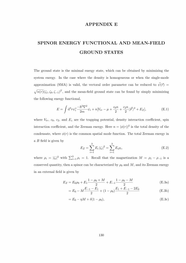
APPENDIX E

SPINOR ENERGY FUNCTIONAL AND MEAN-FIELD

GROUND STATES

The ground state is the minimal energy state, which can be obtained by minimizing the

system energy. In the case where the density is homogeneous or when the single-mode

approximation (SMA) is valid, the vectoral order parameter can be reduced to ~ψ(~r) =√

n(r)(ζ1, ζ0, ζ−1)T , and the mean-field ground state can be found by simply minimizing

the following energy functional,

E =∫

d3rψ∗i−~2∇2

2mψi + n[Vtr − µ +

c0n

2+

c2n

2〈~F 〉2 + EZ ], (E.1)

where Vtr, c0, c2, and Ez are the trapping potential, density interaction coefficient, spin

interaction coefficient, and the Zeeman energy. Here n = |φ(r)|2 is the total density of the

condensate, where φ(r) is the common spatial mode function. The total Zeeman energy in

a B field is given by

EZ =3∑

i=1

Ei |ζi|2 =3∑

i=1

Eiρi, (E.2)

where ρi = |ζi|2 with∑3

i=1 ρi = 1. Recall that the magnetization M = ρ1 − ρ−1 is a

conserved quantity, then a spinor can be characterized by ρ0 and M , and its Zeeman energy

in an external field is given by

EZ = E0ρ0 + E11− ρ0 + M

2+ E−1

1− ρ0 −M

2(E.3a)

= E0 −ME−1 −E1

2+ (1− ρ0)

E1 + E−1 − 2E0

2(E.3b)

= E0 − ηM + δ(1− ρ0), (E.3c)

130

where η = (E−1 − E1)/2 is the linear Zeeman shift, and δ = (E1 + E−1 − 2E0)/2 is the

quadratic Zeeman shift. However,

〈Fz〉 = M, (E.4)

〈F 2z 〉 = |ζ1|2 + |ζ−1|2 = 1− ρ0. (E.5)

By substitution, the Zeeman energy can be expressed as

EZ = E0 − η〈Fz〉+ δ〈F 2z 〉. (E.6)

To account for the conservation of particle number and magnetization in Eq. (E.1), one can

introduce two Lagrange multipliers µ and η0. With a homogeneous density or under SMA,

the ground state structure is determined by the spin-dependent (anti-symmetric) part of

the energy functional,

K =∫

d3~rn[c2n

2〈~F 〉2 − η〈Fz〉+ δ〈F 2

z 〉] (E.7a)

=c

2〈~F 〉2 − η〈Fz〉+ δ〈F 2

z 〉, (E.7b)

where c = c2

∫d3r n(r)2, and η = η + η0. To further simplify this spin-dependent energy

functional, we recall that

〈Fx〉2 =12(ζ∗1ζ0 + ζ∗0ζ1 + ζ∗0ζ−1 + ζ∗−1ζ0)2,

〈Fy〉2 = −12(−ζ∗1ζ0 + ζ∗0ζ1 − ζ∗0ζ−1 + ζ∗−1ζ0)2,

〈Fz〉2 = (|ζ1|2 − |ζ−1|2)2 = M2,

〈F 2z 〉 = |ζ1|2 + |ζ−1|2 = 1− ρ0,

where ρi = |ζi|2 with∑3

i=1 ρi = 1, and M = ρ1 − ρ−1. Then

〈F 〉2 = 〈Fx〉2 + 〈Fy〉2 + 〈Fz〉2 (E.8a)

= 2(ζ∗1ζ0 + ζ∗0ζ−1)(ζ∗0ζ1 + ζ∗−1ζ0) + (|ζ1|2 − |ζ−1|2)2 (E.8b)

= 2(ρ1ρ0 + ζ∗20 ζ1ζ−1 + ζ2

0ζ∗1ζ∗−1 + ρ−1ρ0

)+ M2 (E.8c)

= 2 (ρ1ρ0 + 2ρ0√

ρ1ρ−1 cos θ + ρ−1ρ0) + M2. (E.8d)

131

Here we let ζi =√

ρi eθi , and we define the spinor phase to be θ ≡ θ1+θ−1−2θ0. Minimizing

c〈F 〉2 requires

θ = 0, c < 0, (E.9)

θ = π, c > 0. (E.10)

Therefore,

〈F 〉2 = 2ρ0(√

ρ1 ±√ρ−1)2 + M2 (E.11a)

= 2ρ0

[(1− ρ0)±

√(1− ρ0)2 −M2

]+ M2, (E.11b)

where “+” and “−” signs are for c < 0 and c > 0. Substitute back to Eq. (E.7), the spinor

energy function is found as

K = cρ0

[(1− ρ0 ±

√(1− ρ0)2 −M2

]+

c

2M2 − ηM + δ(1− ρ0). (E.12)

This is reminiscent of Eq. (5.28), with two additional terms, c2M2 − ηM . These additional

terms were omitted in Eq. (5.28) under conservation of magnetization. In a field with

large gradient along the z direction, η = η(z) = gF µBB′z, where gF is the Lande g-factor

for electron, and µB is the Bohr magneton, the gradient will exert magnetic forces on m1

and m−1 components and cause them to separate in space. In this circumstance, SMA

is invalid and conservation of local magnetization does not hold. The ground state then

presents a domain structure, and this structure can be found by minimizing Eq. (E.11)

without conservation of magnetization. This kind of domain structures formed due to high

field gradient has been observed by the MIT group in the anti-ferromagnetic Na F = 1

condensates [42].

When the field gradient is small such that the SMA is valid, the magnetization is con-

served and minimization of K leads to the mean-field ground state in ref. [112]. In this

thesis, the ground states we observed in the 87Rb ferromagnetic F = 1 condensates are

under validity of SMA and conservation of magnetization.

132

APPENDIX F

PROCEDURE FOR EXTRACTING C 2

As discussed in Chapter 3 , the density and the chemical potential of the condensate are often

computed from the measured number of atoms, N , and the trap frequency, ω = (ωxωyωz)1/3.

Recall from Eqs. (3.28) and (3.32), the peak density is given as n0 = µ/g, where g =

4π~2a/m = c0 is the mean-field density interaction strength, and µ = (15~2m1/2

25/2 Nω3a)2/5

is the chemical potential. Here a = (2aF=2 + aF=0)/3 is the averaged s-wave scattering

length. However, measuring the trap frequencies and the absolute number of atoms in

the condensate to within 15% are challenging. First, the parametric excitation technique

that are used for measuring the trap frequencies is likely to excite superfluid modes of a

condensate, which is not an integer multiple of the trap frequencies [28, 29]. Secondly, the

trap depth is very shallow, typically 1 µK, and the trap frequencies are very low, which are

more difficult to determine in general. On the other hand, measuring absolute number of

atoms is always challenging. This is because an accurate measure of the imaging system

efficiency is difficult to obtain. In addition, and absorption imaging can be affected by

a stray field, since the optical transition (|F = 2,mF = 2〉 ↔ |F ′ = 3,mF = 3〉)is field

sensitive.

Alternatively, one can measure the density or the chemical potential directly from the

expansion rate of condensates. Recall from Eq. 3.35a, when the reduced expansion time

τ satisfies τ = t · ω⊥ À 1, where t is the expansion time and ω⊥ is the trap frequency

along the tight trap direction, the condensate radius is R(t) '√

2µm t = kt. Here we define

the expansion rate (slope) k =√

2µ/m. With the measured k, the chemical potential

can be computed as µ = k2m/2. To extract c, we measure the oscillation frequencies vs.

populations, and then fit these data points to the theory, c√

1− ρ20 [114, 117], with free

parameter c. Given that c ≡ c2N∫ |φ|4d3r, where N is the total number of atoms, the spin

133

80

60

40

20

0

Con

dens

ate

Rad

ius

(µm

)

20151050

Expansion time (ms)

Figure F.1: BEC radius vs. expansion time. Measuring the expansion rate allows directmeasurement of density. The solid curves are the theoretical predictions with 10 µm ofimaging resolution, and the solid circles are the measured data. The theoretical predictionsare deconvoluted from the imaging resolution and then fitted with a linear function to findthe the slop k. The fitted slops are kmax = 4.1 µm/ms and kmin = 3.6 µm/ms. Thedeviation between the data and the theoretical predictions near time zero are due to thatthe optical densities are too high to measure the condensate radius correctly. In order toreduce the optical density, the absorption probe detuning is -5 MHz before 5 ms of droptime and -3 MHz after that.

interaction coefficient c2 can be calculated as

c2 =c

N∫ |φ|4d3r

=72

c0c

k2m. (F.1)

Here the averaged condensate density is given by,

N

∫|φ|4d3r =

47n0 =

47

µ

g=

27

k2m

c0, (F.2)

where n0 = µ/g is the peak density, and g = (4π~2/m)a = c0 is the density mean-field

interaction strength. The details for finding the above integral will be given below.

With the measured k = 3.9(4) µm/ms, the averaged condensate density is calculated to

be n0 = 2.1(4)×1014 cm−3. Together with the measured c = 4.3(3) Hz, the spin-dependent

interaction coefficient is found to be c2 = −3.6(8) × 10−14 Hz/cm3 or the difference of

scattering lengthes ∆a = a2 − a0 = −1.4(3) Bohr. Note that the negative sign of c2

is not determined by the measurements here, but was determined from studies of spinor

ground states and from the miscibilities of different spin components which are shown in

Chapter 6-8.

134

Computation of∫ |φ|4d3r The normalized Thomas-Fermi density profile is given by

1N

n(r) = |φ|2 =1

Ngmax[(µ− 1

2mω2r2), 0],

where n(r) is the condensate density, N is the total number of atoms, and g = 4π~2m a = c0.

The condensate radius R is calculated as

R =

(15Nc0

8π 12mω2

)1/5

, (F.3)

which is solved by substituting the equation µ = 12mω2R2 into the normalization integral,

∫ R0 |φ|2 d3r = 1. That is

∫ R

0|φ|2 d3r =

1Nc0

12mω2

∫ R

0(R2 − r2)4πr2dr

=4πmω2R5

15Nc0

= 1.

Given µ = 12mω2R2, we also find that R3 = 15Nc0

8πµ . Substitute R into the following integral,

∫|φ|4 d3r = 4π(

12mω2

Nc0)2

∫ R

0(R2 − r2)2r2dr

= 4π(158π

)28

105R−3

=47

µ

Nc0.

From the above intetral, it is readily found that

N

∫|φ|4d3r =

47

µ

c0=

47n0,

where the peak density n0 = µ/c0.

135

REFERENCES

[1] M. H. Anderson, J. R. Ensher, M. R. Matthews, C. E. Wieman, and E. A. Cornell,“Observation of Bose-Einstein Condensation in a Dilute Atomic Vapor,” Science 269,198 (1995).

[2] C. C. Bradley, C. A. Sackett, J. J. Tollett, and R. G. Hulet, “Evidence of Bose-Einstein Condensation in an Atomic Gas with Attractive Interactions,” Phys. Rev.Lett. 75, 1687 (1995).

[3] K. B. Davis et al., “Bose-Einstein Condensation in a Gas of Sodium Atoms,” Phys.Rev. Lett. 75, 3969 (1995).

[4] W. C. Stwalley and L. H. Nosanow, “Possible New Quantum Systems,” Phys. Rev.Lett. 36, 910 (1976).

[5] I. F. Silvera and J. T. M. Walraven, “Stabilization of Atomic-Hydrogen at Low-Temperature,” Phys. Rev. Lett. 44, 164 (1980).

[6] E. L. Raab, M. Prentiss, A. Cable, S. Chu, and D. E. Pritchard, “Trapping of NeutralSodium Atoms with Radiation Pressure,” Phys. Rev. Lett. 59, 2631 (1987).

[7] C. Monroe, W. Swann, H. Robinson, and C. Wieman, “Very Cold Trapped Atoms ina Vapor Cell,” Phys. Rev. Lett. 65, 1571 (1990).

[8] E. A. Cornell, J. R. Ensher, and C. E. Wieman, “Experiments in dilute atomic Bose-Einstein condensation,” in International School of Physics “Enrico Fermi”, CourseCXL, edited by M. Inguscio, S. Stringari, and C. E. Wieman Varenna, Lake Como,Italy 1999 IOS Press.

[9] W. Ketterle, D. S. Durfee, and D. M. Stamper-Kurn, “Making, probing and under-standing Bose-Einstein condensates (cond-mat/9904034),” in International School ofPhysics “Enrico Fermi”, Course CXL, edited by M. Inguscio, S. Stringari, and C. E.Wieman Varenna, Lake Como, Italy 1999 IOS Press.

[10] M. R. Andrews et al., “Observation of interference between two Bose condensates,”Science 275, 637 (1997).

[11] I. Bloch, T. W. Hansch, and T. Esslinger, “measurement of the spatial coherence ofa trapped bose gas at the phase transition,” Nature 403, 166 (2000).

[12] B. P. Anderson and M. A. Kasevich, “Macroscopic quantum interference from atomictunnel arrays,” Science 282, 1686 (1998).

[13] M. Albiez et al., “Direct observation of tunneling and nonlinear self-trapping in asingle bosonic Josephson junction,” Phys. Rev. Lett. 95, 010402 (2005).

136

[14] M. Greiner, O. Mandel, T. Esslinger, T. W. Hansch, and I. Bloch, “Quantum phasetransition from a superfluid to a Mott insulator in a gas of ultracold atoms,” Nature415, 39 (2002).

[15] M. O. Mewes et al., “Output coupler for Bose-Einstein condensed atoms,” Phys. Rev.Lett. 78, 582 (1997).

[16] E. W. Hagley et al., “A well-collimated quasi-continuous atom laser,” Science 283,1706 (1999).

[17] I. Bloch, T. W. Hansch, and T. Esslinger, “Atom laser with a cw output coupler,”Phys. Rev. Lett. 82, 3008 (1999).

[18] E. A. Burt et al., “Coherence, correlations, and collisions: What one learns aboutBose-Einstein condensates from their decay,” Phys. Rev. Lett. 79, 337 (1997).

[19] S. Folling et al., “Spatial quantum noise interferometry in expanding ultracold atomclouds,” Nature 434, 481 (2005).

[20] G. Baym and C. J. Pethick, “Ground-state properties of magnetically trapped Bose-condensed rubidium gas,” Phys. Rev. Lett. 76, 6 (1996).

[21] F. Dalfovo and S. Stringari, “Bosons in anisotropic traps: Ground state and vortices,”Phys. Rev. A 53, 2477 (1996).

[22] C. C. Bradley, C. A. Sackett, and R. G. Hulet, “Bose-Einstein condensation of lithium:Observation of limited condensate number,” Phys. Rev. Lett. 78, 985 (1997).

[23] E. A. Donley et al., “Dynamics of collapsing and exploding Bose-Einstein conden-sates,” Nature 412, 295 (2001).

[24] C. J. Pethick and H. Smith, Bose-Einstein Condensation in Dilute Gases (CambridgeUniversity Press, Cambridge, UK, 2002).

[25] M. R. Matthews et al., “Vortices in a Bose-Einstein condensate,” Phys. Rev. Lett.83, 2498 (1999).

[26] K. Madison, F. Chevy, W. Wohlleben, and J. Dalibard, “Vortex Formation in aStirred Bose-Einstein Condensate,” Phys. Rev. Lett. 84, 806 (2000).

[27] J. R. Abo-Shaeer, C. Raman, J. M. Vogels, and W. Ketterle, “Observation of vortexlattices in Bose-Einstein condensates,” Science 292, 476 (2001).

[28] D. S. Jin, J. R. Ensher, M. R. Matthews, C. E. Wieman, and E. A. Cornell, “CollectiveExcitations of a Bose-Einstein Condensate in a Dilute Gas,” Phys. Rev. Lett. 77, 420(1996).

[29] M. O. Mewes et al., “Collective excitations of a Bose-Einstein condensate in a mag-netic trap,” Phys. Rev. Lett. 77, 988 (1996).

[30] M. R. Andrews et al., “Propagation of sound in a Bose-Einstein condensate,” Phys.Rev. Lett. 79, 553 (1997).

137

[31] S. Burger et al., “Dark solitons in Bose-Einstein condensates,” Phys. Rev. Lett. 83,5198 (1999).

[32] J. Denschlag et al., “Generating solitons by phase engineering of a Bose-Einsteincondensate,” Science 287, 97 (2000).

[33] K. E. Strecker, G. B. Partridge, A. G. Truscott, and R. G. Hulet, “Formation andpropagation of matter-wave soliton trains,” Nature 417, 150 (2002).

[34] M. D. Barrett, J. A. Sauer, and M. S. Chapman, “All-optical formation of an atomicBose-Einstein condensate,” Phys. Rev. Lett. 87, 010404 (2001).

[35] D. M. Stamper-Kurn et al., “Optical confinement of a Bose-Einstein condensate,”Phys. Rev. Lett. 80, 2027 (1998).

[36] Y. Takasu et al., “Spin-singlet Bose-Einstein condensation of two-electron atoms,”Phys. Rev. Lett. 91, 040404 (2003).

[37] W. Hansel, P. Hommelhoff, T. W. Hansch, and J. Reichel, “Bose-Einstein condensa-tion on a microelectronic chip,” Nature 413, 498 (2001).

[38] H. Ott, J. Fortagh, G. Schlotterbeck, A. Grossmann, and C. Zimmermann, “Bose-Einstein condensation in a surface microtrap,” Phys. Rev. Lett. 8723, 230401 (2001).

[39] T. L. Ho, “Spinor Bose condensates in optical traps,” Phys. Rev. Lett. 81, 742 (1998).

[40] T. Ohmi and K. Machida, “Bose-Einstein condensation with internal degrees of free-dom in alkali atom gases,” J. Phys. Soc. Jpn. 67, 1822 (1998).

[41] C. J. Myatt, E. A. Burt, R. W. Ghrist, E. A. Cornell, and C. E. Wieman, “Productionof two overlapping Bose-Einstein condensates by sympathetic cooling,” Phys. Rev.Lett. 78, 586 (1997).

[42] J. Stenger et al., “Spin domains in ground-state Bose-Einstein condensates,” Nature396, 345 (1998).

[43] A. Grlitz et al., “Sodium Bose-Einstein condensates in the F=2 state in a large-volumeoptical trap,” Phys. Rev. Lett. 90, 010404 (2003).

[44] H. Schmaljohann et al., “Dynamics of F=2 spinor Bose-Einstein condensates,” Phys.Rev. Lett. 92, 040402 (2004).

[45] M. S. Chang et al., “Observation of spinor dynamics in optically trapped Rb-87Bose-Einstein condensates,” Phys. Rev. Lett. 92, 140403 (2004).

[46] A. J. Leggett, “Theoretical Description of New Phases of Liquid-He-3,” Rev. Mod.Phys. 47, 331 (1975).

[47] J. C. Wheatley, “Experimental Properties of Superfluid He-3,” Rev. Mod. Phys. 47,415 (1975).

[48] D. J. Dean and M. Hjorth-Jensen, “Pairing in nuclear systems: from neutron starsto finite nuclei,” Rev. Mod. Phys. 75, 607 (2003).

138

[49] A. P. M. Maeno and Y., “The superconductivity of Sr2RuO4 and the physics ofspin-triplet pairing,” Rev. Mod. Phys. 75, 657 (2003).

[50] C. V. Ciobanu, S. K. Yip, and T. L. Ho, “Phase diagrams of F=2 spinor Bose-Einsteincondensates,” Phys. Rev. A 61, 033607 (2000).

[51] E. A. Cornell, D. S. Hall, M. R. Matthews, and C. E. Wieman, “Having it both ways:Distinguishable yet phase-coherent mixtures of Bose-Einstein condensates,” J. LowTemp. Phys. 113, 151 (1998).

[52] H. J. Miesner et al., “Observation of metastable states in spinor Bose-Einstein con-densates,” Phys. Rev. Lett. 82, 2228 (1999).

[53] D. M. Stamper-Kurn et al., “Quantum tunneling across spin domains in a Bose-Einstein condensate,” Phys. Rev. Lett. 83, 661 (1999).

[54] C. K. Law, H. Pu, and N. P. Bigelow, “Quantum spins mixing in spinor Bose-Einsteincondensates,” Phys. Rev. Lett. 81, 5257 (1998).

[55] N. N. Klausen, J. L. Bohn, and C. H. Greene, “Nature of spinor Bose-Einsteincondensates in rubidium,” Phys. Rev. A 64, 053602 (2001).

[56] E. G. M. van Kempen, S. J. J. M. F. Kokkelmans, D. J. Heinzen, and B. J. Ver-haar, “Interisotope determination of ultracold rubidium interactions from three high-precision experiments,” Phys. Rev. Lett. 88, 093201 (2002).

[57] D. A. Steck, “Rubidium 87 D Line Data,” (2003).

[58] J. Vanier and C. Audoin, The quantum physics of atomic frequency standards (A.Hilger, Philadelphia, 1988).

[59] H. J. Metcalf and P. van der Straten, Laser Cooling and Trapping (Springer-Verlag,New York, 1999).

[60] K. B. Macadam, A. Steinbach, and C. Wieman, “A Narrow-Band Tunable Diode-Laser System with Grating Feedback, and a Saturated Absorption Spectrometer forCs and Rb,” Am. J. Phys. 60, 1098 (1992).

[61] W. Demtroder, Laser Spectroscopy, 2nd ed. (Springer, New York, 1996).

[62] M. D. Barrett, A Quest for BEC: An all-optical alternative, PhD thesis GeorgiaInstitute of Technology 2002.

[63] C. C. Bradley, J. Chen, and R. G. Hulet, “Instrumentation for the Stable Operationof Laser-Diodes,” Rev. Sci. Inst. 61, 2097 (1990).

[64] C. E. Wieman and L. Hollberg, “Using Diode-Lasers for Atomic Physics,” Rev. Sci.Inst. 62, 1 (1991).

[65] K. G. Libbrecht and J. L. Hall, “A Low-Noise High-Speed Diode-Laser CurrentController,” Rev. Sci. Inst. 64, 2133 (1993).

[66] S. Friebel, R. Scheunemann, J. Walz, T. W. Hansch, and M. Weitz, “Laser cooling ina CO2-laser optical lattice,” Appl. Phy. B 67, 699 (1998).

139

[67] J. D. Jackson, Classical Electrodynamics, 2nd ed. (Willey, New York, 1975).

[68] E. A. Cornell, J. R. Ensher, and C. E. Wieman, “Experiments in dilute atomicBose-Einstein condensation (cond-mat/9903109),” in International School of Physics“Enrico Fermi” on Bose-Einstein Condensation in Atomic Gases, edited by M. In-guscio, S. Stringari, and C. E. Wieman p. 15 IOS Press 1998.

[69] S. Chu, J. E. Bjorkholm, A. Ashkin, and A. Cable, “Experimental Observation ofOptically Trapped Atoms,” Phys. Rev. Lett. 57, 314 (1986).

[70] C. S. Adams, H. J. Lee, N. Davidson, M. Kasevich, and S. Chu, “Evaporative Coolingin a Crossed Dipole Trap,” Phys. Rev. Lett. 74, 3577 (1995).

[71] T. Takekoshi, J. R. Yeh, and R. J. Knize, “Quasi-electrostatic trap for neutral atoms,”Opt. Comm. 114, 421 (1995).

[72] R. Grimm, M. Weidemuller, and Y. B. Ovchinnikov, “Optical dipole traps for neutralatoms,” Adv. Atom. Mol. Opt. Phys. 42, 95 (2000).

[73] D. J. Han, M. T. DePue, and D. S. Weiss, “Loading and compressing Cs atoms in avery far-off-resonant light trap,” Phy. Rev. A 6302, 023405 (2001).

[74] A. Robert et al., “A Bose-Einstein Condensate of Metastable Atoms,” Science 292,461 (2001).

[75] H. Haken and H. C. Wolf, Molecular Physics and Elements of Quantum Chemistry(Springer, Berlin, 1995).

[76] F. Reif, Fundametals of Statistical and Thermal Physics (McGraw Hill, New York,1965).

[77] S. Friebel, C. D’Andrea, J. Walz, M. Weitz, and T. W. Hansch, “CO2-laser opticallattice with cold rubidium atoms,” Phy. Rev. A 57, R20 (1998).

[78] V. I. Arnold, Mathemtaical Methods of Classical Mechanics, 2nd ed. (Springer-Verlag,New York, 1988).

[79] F. Dalfovo, L. Pitaevskii, and S. Stringari, “Order parameter at the boundary of atrapped Bose gas,” Phys. Rev. A 54, 4213 (1996).

[80] Y. Castin and R. Dum, “Bose-Einstein condensates in time dependent traps,” Phys.Rev. Lett. 77, 5315 (1996).

[81] F. Gerbier et al., “Experimental study of the thermodynamics of an interactingtrapped Bose-Einstein condensed gas,” Phy. Rev. A 70, 013607 (2004).

[82] G. Cennini, G. Ritt, C. Geckeler, and M. Weitz, “All-optical realization of an atomlaser,” Phys. Rev. Lett. 91, 240408 (2003).

[83] T. Kinoshita, T. Wenger, and S. Weiss, David, “All-optical Bose-Einstein condensa-tion using a compressible crossed dipole trap,” Phys. Rev. A 71, 011602 (2005).

[84] T. Weber, J. Herbig, M. Mark, H. C. Nagerl, and R. Grimm, “Bose-Einstein conden-sation of cesium,” Science 299, 232 (2003).

140

[85] W. D. Phillips 2005.

[86] S. R. Granade, M. E. Gehm, K. M. O’Hara, and J. E. Thomas, “All-optical productionof a degenerate Fermi gas,” Phys. Rev. Lett. 88, 120405 (2002).

[87] R. Scheunemann, F. S. Cataliotti, T. W. Hansch, and M. Weitz, “An optical latticewith single lattice site optical control for quantum engineering,” J. Opt. B 2, 645(2000).

[88] J. H. Denschlag et al., “A Bose-Einstein condensate in an optical lattice,” J. Phys. B35, 3095 (2002).

[89] D. Jaksch, H. J. Briegel, J. I. Cirac, C. W. Gardiner, and P. Zoller, “Entanglementof atoms via cold controlled collisions,” Phys. Rev. Lett. 82, 1975 (1999).

[90] G. K. Brennen, C. M. Caves, F. S. Jessen, and I. H. Deutsch, “Quantum logic gatesin optical lattices,” Phys. Rev. Lett. 82, 1060 (1999).

[91] S. Kuhr et al., “Deterministic delivery of a single atom,” Science 293, 278 (2001).

[92] J. A. Sauer, K. M. Fortier, M. S. Chang, C. D. Hamley, and M. S. Chapman, “CavityQED with optically transported atoms,” Phy. Rev. A 69, 051804 (2004).

[93] S. Chu, “The manipulation of neutral particles,” Rev. Mod. Phys. 70, 685 (1998).

[94] W. D. Phillips, “Laser cooling and trapping of neutral atoms,” Rev. Mod. Phys. 70,721 (1998).

[95] T. A. Savard, K. M. OHara, and J. E. Thomas, “Laser-noise-induced heating in far-offresonance optical traps,” Phy. Rev. A 56, R1095 (1997).

[96] M. E. Gehm, K. M. O’Hara, T. A. Savard, and J. E. Thomas, “Dynamics of noise-induced heating in atom traps,” Phy. Rev. A 58, 3914 (1998).

[97] T. Ido, Y. Isoya, and H. Katori, “Optical-dipole trapping of Sr atoms at a highphase-space density,” Phys Rev A 61, 061403 (2000).

[98] T. Takekoshi and R. J. Knize, “CO2 laser trap for cesium atoms,” Opt. Lett. 21, 77(1996).

[99] S. J. M. Kuppens, K. L. Corwin, K. W. Miller, T. E. Chupp, and C. E. Wieman,“Loading an optical dipole trap,” Phy. Rev. A 62, 013406 (2000).

[100] K. M. O’Hara, S. R. Granade, M. E. Gehm, and J. E. Thomas, “Loading dynamicsof CO2 laser traps,” Phy. Rev. A 63, 043403 (2001).

[101] Y. Takasu et al., “High-density trapping of cold ytterbium atoms by an optical dipoleforce,” Phys. Rev. Lett. 90, 023003 (2003).

[102] C. Orzel, A. K. Tuchman, M. L. Fenselau, M. Yasuda, and M. A. Kasevich, “Squeezedstates in a Bose-Einstein condensate,” Science 291, 2386 (2001).

[103] W. K. Hensinger et al., “Dynamical tunnelling of ultracold atoms,” Nature 412, 52(2001).

141

[104] F. S. Cataliotti et al., “Josephson junction arrays with Bose-Einstein condensates,”Science 293, 843 (2001).

[105] M. Greiner, O. Mandel, T. W. Hansch, and I. Bloch, “Collapse and revival of thematter wave field of a Bose-Einstein condensate,” Nature 419, 51 (2002).

[106] D. C. O’Shea, Elements of modern optical design (Wiley, New York, 1985).

[107] K. B. Davis, M. O. Mewes, and W. Ketterle, “An Analytical Model for EvaporativeCooling of Atoms,” Appl. Phys. B 60, 155 (1995).

[108] D. S. Hall, M. R. Matthews, J. R. Ensher, C. E. Wieman, and E. A. Cornell, “Dy-namics of component separation in a binary mixture of Bose-Einstein condensates,”Phys. Rev. Lett. 81, 1539 (1998).

[109] D. S. Hall, M. R. Matthews, C. E. Wieman, and E. A. Cornell, “Measurements ofrelative phase in two-component Bose-Einstein condensates,” Phys. Rev. Lett. 81,1543 (1998).

[110] J. E. Williams and M. J. Holland, “Preparing topological states of a Bose-Einsteincondensate,” Nature 401, 568 (1999).

[111] M. Koashi and M. Ueda, “Exact eigenstates and magnetic response of spin-1 andspin-2 Bose-Einstein condensates,” Phys. Rev. Lett. 84, 1066 (2000).

[112] W. X. Zhang, S. Yi, and L. You, “Mean field ground state of a spin-1 condensate ina magnetic field,” New J. Phys. 5, 77 (2003).

[113] E. V. Goldstein and P. Meystre, “Quantum theory of atomic four-wave mixing inBose-Einstein condensates,” Phys. Rev. A 59, 3896 (1999).

[114] H. Pu, C. K. Law, S. Raghavan, J. H. Eberly, and N. P. Bigelow, “Spin-mixingdynamics of a spinor Bose-Einstein condensate,” Phys. Rev. A 60, 1463 (1999).

[115] J. P. Burke, P. S. Julienne, C. J. Williams, Y. B. Band, and M. Trippenbach, “Four-wave mixing in Bose-Einstein condensate systems with multiple spin states,” Phys.Rev. A 70, 033606 (2004).

[116] D. R. Romano and E. J. V. de Passos, “Population and phase dynamics of F=1 spinorcondensates in an external magnetic field,” Phys. Rev. A 70, 043614 (2004).

[117] W. Zhang, D. L. Zhou, M.-S. Chang, M. S. Chapman, and L. You, “Coherent spinmixing dynamics in a spin-1 atomic condensate,” Phys. Rev. A 72, 013602 (2005).

[118] A. E. Leanhardt, Y. Shin, D. Kielpinski, D. E. Pritchard, and W. Ketterle, “Corelessvortex formation in a spinor Bose-Einstein condensate,” Phys. Rev. Lett. 90, 140403(2003).

[119] T. Isoshima, K. Machida, and T. Ohmi, “Spin-domain formation in spinor Bose-Einstein condensation,” Phys. Rev. A 60, 4857 (1999).

[120] L. M. Duan, J. I. Cirac, and P. Zoller, “Quantum entanglement in spinor Bose-Einsteincondensates,” Phys. Rev. A 65, 033619 (2002).

142

[121] H. Pu and P. Meystre, “Creating macroscopic atomic Einstein-Podolsky-Rosen statesfrom Bose-Einstein condensates,” Phys. Rev. Lett. 85, 3987 (2000).

[122] J. P. Burke, C. H. Greene, and J. L. Bohn, “Multichannel cold collisions: Simpledependences on energy and magnetic field,” Phys. Rev. Lett. 81, 3355 (1998).

[123] D. Stamper-Kurn and W. Ketterle, “Spinor Condensates and Light Scattering FromBose-Einstein Condensates (cond-mat/0005001 v1 29),” in Les Houches SummerSchool, Section LXXII, edited by R. Kaiser, C. Westbrook, and F. David pp. 139–208Les Houches, France 1999 Springer, Berlin.

[124] H. Pu, S. Raghavan, and N. P. Bigelow, “Manipulating spinor condensates withmagnetic fields: Stochastization, metastability, and dynamical spin localization,” Phy.Rev. A 61, 023602 (2000).

[125] T. Kuwamoto, K. Araki, T. Eno, and T. Hirano, “Magnetic field dependence ofthe dynamics of Rb-87 spin-2 Bose-Einstein condensates,” Phys. Rev. A 69, 063604(2004).

[126] M. R. Matthews et al., “Watching a superfluid untwist itself: Recurrence of rabioscillations in a Bose-Einstein condensate,” Phys. Rev. Lett. 83, 3358 (1999).

[127] S. Yi, O. E. Mustecaplioglu, C. P. Sun, and L. You, “Single-mode approximation ina spinor-1 atomic condensate,” Phy. Rev. A 66, 011601 (2002).

[128] A. Barone and G. Paterno, Physics and applications of the Josephson effect (Wiley,New York, 1982).

[129] J. Javanainen, “Oscillatory Exchange of Atoms between Traps Containing Bose Con-densates,” Phys. Rev. Lett. 57, 3164 (1986).

[130] A. Smerzi, S. Fantoni, S. Giovanazzi, and S. R. Shenoy, “Quantum coherent atomictunneling between two trapped Bose-Einstein condensates,” Phys. Rev. Lett. 79, 4950(1997).

[131] J. C. Davis and R. E. Packard, “Superfluid 3He weak links,” Rev. Mod. Phys. 74,741 (2001).

[132] L. You, “Creating Maximally Entangled Atomic States in a Bose-Einstein Conden-sate,” Phys. Rev. Lett. 90, 030402 (2003).

[133] M. Erhard, H. Schmaljohann, J. Kronjager, K. Bongs, and K. Sengstock, “Bose-Einstein condensation at constant temperature,” Phy. Rev. A 70, 031602 (2004).

[134] T. Isoshima, T. Ohmi, and K. Machida, “Double phase transitions in magnetizedspinor Bose-Einstein condensation,” J. Phy. Soc. Jpn. 69, 3864 (2000).

[135] W. X. Zhang, S. Yi, and L. You, “Bose-Einstein condensation of trapped interactingspin-1 atoms,” Phy. Rev. A 70, 043611 (2004).

[136] M. D. Barrett et al., “All-Optical Atomic Bose-Einstein Condensates,” in XVIIIInternational Conference on Atomic Physics, edited by H. R. Sadeghpour, E. J. Heller,and D. E. Pritchard Cambridge, MA, USA 2002 World Scientific.

143

[137] T. L. Ho and S. K. Yip, “Fragmented and single condensate ground states of spin-1Bose gas,” Phys. Rev. Lett. 84, 4031 (2000).

[138] J. R. Ensher, D. S. Jin, M. R. Matthews, C. E. Wieman, and E. A. Cornell, “Bose-Einstein condensation in a dilute gas: Measurement of energy and ground-state oc-cupation,” Phys. Rev. Lett. 77, 4984 (1996).

[139] E. A. Donley, N. R. Claussen, S. T. Thompson, and C. E. Wieman, “Atom-moleculecoherence in a Bose-Einstein condensate,” Nature 417, 529 (2002).

[140] M. Greiner, C. A. Regal, and D. S. Jin, “Emergence of a molecular Bose-Einsteincondensate from a Fermi gas,” Nature 426, 537 (2003).

[141] M. Tinkham, Introduction to superconductivity, 2nd ed. (McGraw Hill, New York,1996).

[142] S. Shapiro, “Josephson Currents in Superconducting Tunneling: The Effect of Mi-crowaves and Other Observations,” Phys. Rev. Lett. 11, 80 (1963).

[143] L. Deng et al., “Four-wave mixing with matter waves,” Nature 398, 218 (1999).

[144] A. Widera et al., “Coherent collisional spin dynamics in optical lattices,” Phys. Rev.Lett. 95, 190405 (2005).

[145] J. Kronjager et al., “Evolution of a spinor condensate: Coherent dynamics, dephasing,and revivals,” Physical Review A 72, 063619 (2005).

[146] M.-S. Chang, Q. Qin, W. Zhang, L. You, and M.-S. Chang, “Coherent Spinor dy-namics in a spin-1 Bose condensate,” Nature Physics 1, 111 (2005).

[147] G. P. Agrawal, Nonlinear Fiber Optics (Academic Press, Boston, 1989).

[148] N. P. Robins, W. P. Zhang, E. A. Ostrovskaya, and Y. S. Kivshar, “Modulationalinstability of spinor condensates,” Phy. Rev. A 64, 021601 (2001).

[149] P. Ao and S. T. Chui, “Binary Bose-Einstein condensate mixtures in weakly andstrongly segregated phases,” Phys. Rev. A 58, 4836 (1998).

[150] W. Zhang, D. L. Zhou, M.-S. Chang, M. S. Chapman, and L. You, “Dynamicalinstability and domain formation in a spin-1 Bose condensate,” Phys. Rev. Lett. 95,180403 (2005).

[151] H. Saito and M. Ueda, “Spontaneous magnetization and structure formation in aspin-1 ferromagnetic Bose-Einstein condensate,” Phy. Rev. A 72, 023610 (2005).

144