Coast-wide Numerical and Hydrodynamic Model Improvements

Report Submitted to the

Texas Water Development Board

Contract #1004831014

PI: Clint Dawson The University of Texas at Austin

E-mail: clint@ices.utexas.edu Voice: (512) 475-8625

Team Members:

Clint Dawson, Professor

Jennifer Proft, Research Scientist

Adnan Muhammad, Graduate Researcher

September 2012

2

1 Executive Summary The University of Texas Computational Hydraulics Group (CHG) collaboratively developed and verified a comprehensive coast-wide numerical grid for the Texas Water Development Board (TWDB). The resulting grid incorporates all bays, estuaries, waterways, and channels along the Texas coast with sufficient resolution to model the primary hydrodynamic interactions among the different systems. Additionally, we developed subgrids which selectively place higher resolution in primary systems of interest to aid with both coastal and freshwater inflow studies. The grids are based on current finite element technology being developed within the CHG and include additional coastal features and updated bathymetry data whenever available. Furthermore, we validate the grids using the finite element modeling system SELFE (a semi-implicit Eulerian-Lagrangian finite-element model), currently in use by TWDB. Specifically, we setup two scenarios: a Corpus Christi Bay baroclinic test problem defined in a previous report [1], and a broader test problem incorporating the Texas coast-wide grid. The models are to be analyzed for stability, efficiency and validity of results.

2 Project Description TWDB is interested in development of a high resolution, triangular finite-element grid of the Texas coast, which incorporates all bays, estuaries, waterways and channels for use in various hydrodynamic modeling studies conducted by TWDB. In this grid, coastal features are sufficiently resolved to meet modeling and numerical accuracy requirements. The domain is bounded on the north and west by the Texas coastline and is arbitrarily cut in the open ocean while still maintaining primary topological features. The final grid is comprised of 1,209,836 elements and 639,505 nodes. It is well known that a high resolution finite element grid is essential for accurate hydrodynamic modeling efforts (for storm surge examples, see [3] and references therein). Capturing the scales of multiple dynamics can only be achieved in a computationally efficient manner through the use of unstructured grids. The advantages of a high resolution, unstructured grid comes with the high price of grid generation, which is an extremely time-consuming and tedious process requiring numerous small manual adjustments. Indeed, the automated improvement of this process is an active area of research [2]. In what follows, we describe the procedure for development of a coast-wide grid utilizing a semi-automatic meshing product called Surface-water Modeling Solution (SMS). We then describe the setup in SELFE. The application of UTBEST3D model in this study was not pursued due to model efficiency issues. Validation of the models, including both the Corpus Christi Bay test case and the Texas coast-wide model continue to be an active area of research.

3

3 The Surface-water Modeling Solution

In this section, we present a brief overview of the SMS software and its uses in this project, discuss the process of generating the Texas coast-wide and related subgrids, and conclude with suggestions for future work.

3.1 Introduction

The Surface-water Modeling Solution, or SMS, developed by Aquaveo is a multi-dimensional hydrodynamic modeling environment. The surface modeling and design capabilities of SMS include both finite element and finite difference methods. Supported models include RMA2, RMA4, ADCIRC, CGWAVE, STWAVE, BOUSS2D, CMS-FLOW, CMS-Wave, and Genesis models. Furthermore, a generic model interface also is available which can be used to support other models (e.g., SELFE) which have not been officially incorporated. The models included in the software compute a variety of information including bathymetry interpolation and velocity solutions to the shallow-water equations, among others. SMS also can be used to construct 2D and 3D finite element grids of water bodies such as rivers, bays, and other wetland areas. After creating the grid, boundary conditions can be assigned [4].

Our use of SMS in this project was primarily for the purposes of grid development, and a comprehensive Gulf of Mexico grid was used as a basis for construction. Although the development and testing of this gulf-wide grid is currently an active area of research, it has successful been validated in storm surge models [5], among other applications. Pertinent coastal areas are individually extracted, remodeled, interpolated for bathymetry, and subsequently merged into a new Texas coast-wide grid. The following section describes how this detailed and time-consuming process was carried out in a collaborative manner between CHG and TWDB.

3.2 Mesh Development Procedure

The procedure described herein was carried out for all major and minor estuaries included in the final Texas coast-wide grid. We describe the procedure for a single bay but highlight other issues that were encountered while working with different parts of the Texas coast. The following is a list of estuaries that were included in the Texas coast-wide grid:

1) Sabine - Neches 2) Trinity - San Jacinto 3) Brazos River 4) San Bernard River 5) Lavaca - Colorado 6) Guadalupe 7) Mission - Aransas 8) Nueces 9) Laguna Madre

4

10) Rio Grande First, using Google Earth, we visually locate a set of rectangular coordinates within the Gulf of Mexico master grid that enclose the bay of interest. These geographic coordinates then are fed into a FORTRAN program called GridScope which extracts the pertinent portion of the master grid enclosed by these coordinates. The extracted grid from which Galveston Bay and the Trinity-San Jacinto Estuary is shown in Figure 1.

Figure 1. Extracted Grids with coastal regions of Galveston Bay and Sabine Lake

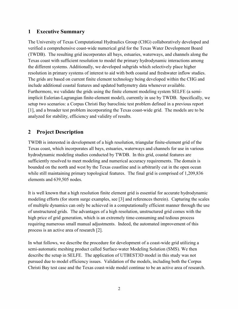
The resulting subgrid of Galveston Bay is then loaded into SMS and saved as a Google Raster file. To verify that the area of interest has been accurately captured by the grid, this raster file is then opened in Google Earth and examined (Figure 2). Should it fail to pass inspection, the process is repeated. The extracted grid carries with it bathymetry information which is used in conjunction with georeferenced aerial images to isolate wet areas from dry ones. These map files are available on the Texas Natural Resources Information System website [6]. Since the files are on the order of several gigabytes in size, there exist lagging issues when working with them. Furthermore, the coordinates are in Universal Transverse Mercator coordinate system (UTM) and thus require conversion of the extracted subgrid from geographic coordinates to UTM coordinate.

5

Figure 2. A Google raster file opened in Google Earth is used to verify that the subgrid, extracted from the Gulf of Mexico-wide master grid, represents the area of interest.

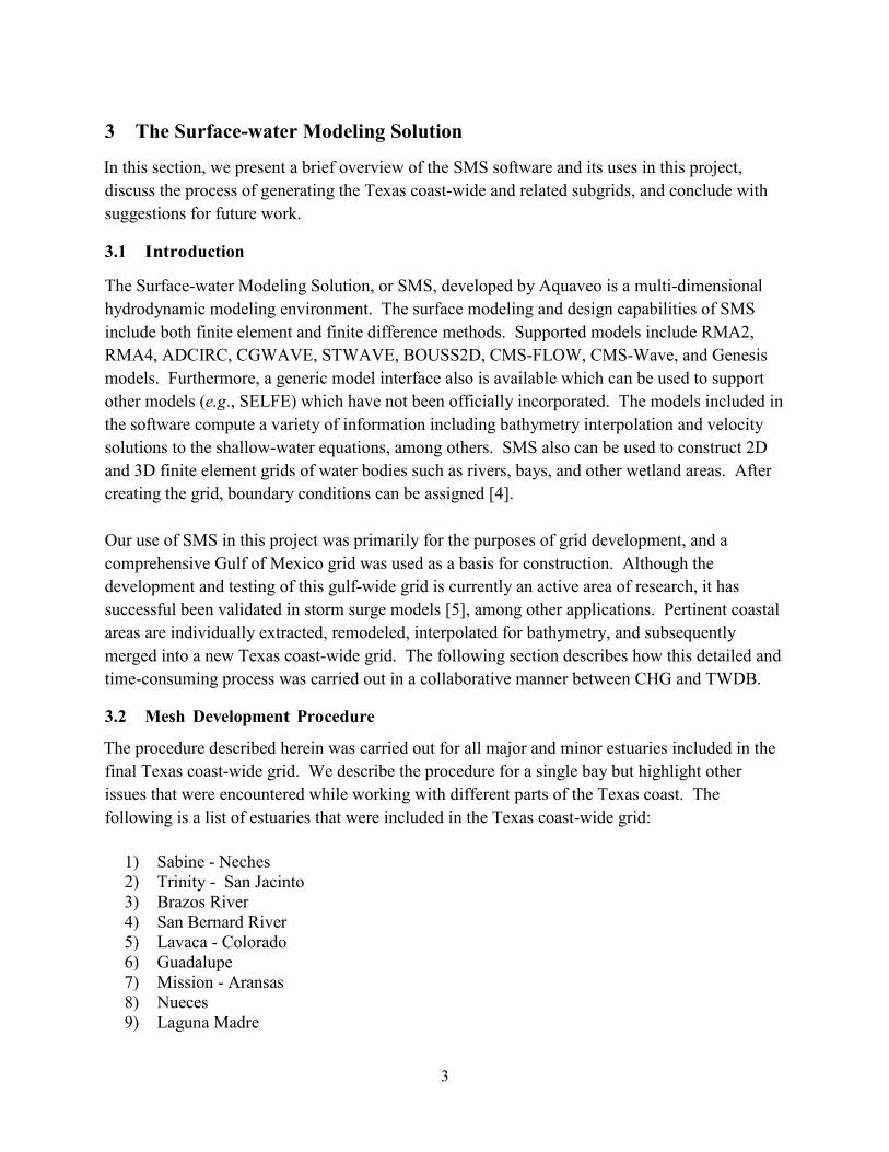
After conversion and loading of the appropriate map file on the background in SMS (Figure 3), we begin the process of drawing nodestrings to isolate wet areas from dry areas. The process of creating nodestrings to isolate these areas is a slow one, since it is necessary to manually switch between different levels of magnification in order to accurately select appropriate nodes. As previously mentioned, the size of the background map is on the order of gigabytes and this necessarily creates a large amount of lag when working with the SMS software. A sample figure with created nodestrings is shown in Figure 4.

Figure 3. Grid for Galveston Bay with background maps from TNRIS.

6

Figure 4. Mesh with nodestrings created for editing purposes.

Nodestrings are important not only for the delineation between wet versus dry regions but also to define polygons in the grid to later be able to re-mesh the area, assign boundary conditions, etc. The creation of nodestrings on this extracted grid is perhaps one of the most time-consuming parts of the process. After nodestrings are created in the SMS software, they are closed so that they can be transformed into arcs which then are turned into polygons (Figure 5). Depending on whether the polygon encloses a wet area or a dry area, nodes and elements are deleted outside and/or inside the polygon. Using the background map image, it is necessary to verify that all rivers, channels, streams and bays shown in the grid bathymetry are indeed within the contour range specifications. The resulting grid now contains only the meshed wet areas (Figure 6).

Figure 5. Polygon built from nodestrings delineating Galveston Bay and Sabine Lake.

7

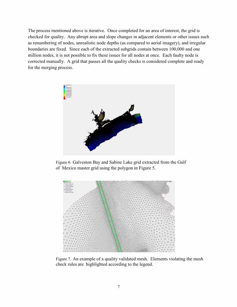
The process mentioned above is iterative. Once completed for an area of interest, the grid is checked for quality. Any abrupt area and slope changes in adjacent elements or other issues such as renumbering of nodes, unrealistic node depths (as compared to aerial imagery), and irregular boundaries are fixed. Since each of the extracted subgrids contain between 100,000 and one million nodes, it is not possible to fix these issues for all nodes at once. Each faulty node is corrected manually. A grid that passes all the quality checks is considered complete and ready for the merging process.

Figure 6. Galveston Bay and Sabine Lake grid extracted from the Gulf of Mexico master grid using the polygon in Figure 5.

Figure 7. An example of a quality validated mesh. Elements violating the mesh check rules are highlighted according to the legend.

8

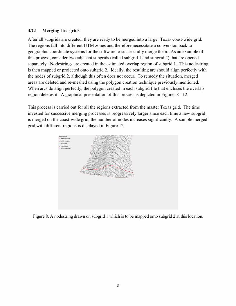
3.2.1 Merging the grids After all subgrids are created, they are ready to be merged into a larger Texas coast-wide grid. The regions fall into different UTM zones and therefore necessitate a conversion back to geographic coordinate systems for the software to successfully merge them. As an example of this process, consider two adjacent subgrids (called subgrid 1 and subgrid 2) that are opened separately. Nodestrings are created in the estimated overlap region of subgrid 1. This nodestring is then mapped or projected onto subgrid 2. Ideally, the resulting arc should align perfectly with the nodes of subgrid 2, although this often does not occur. To remedy the situation, merged areas are deleted and re-meshed using the polygon creation technique previously mentioned. When arcs do align perfectly, the polygon created in each subgrid file that encloses the overlap region deletes it. A graphical presentation of this process is depicted in Figures 8 - 12. This process is carried out for all the regions extracted from the master Texas grid. The time invested for successive merging processes is progressively larger since each time a new subgrid is merged on the coast-wide grid, the number of nodes increases significantly. A sample merged grid with different regions is displayed in Figure 12.

Figure 8. A nodestring drawn on subgrid 1 which is to be mapped onto subgrid 2 at this location.

9

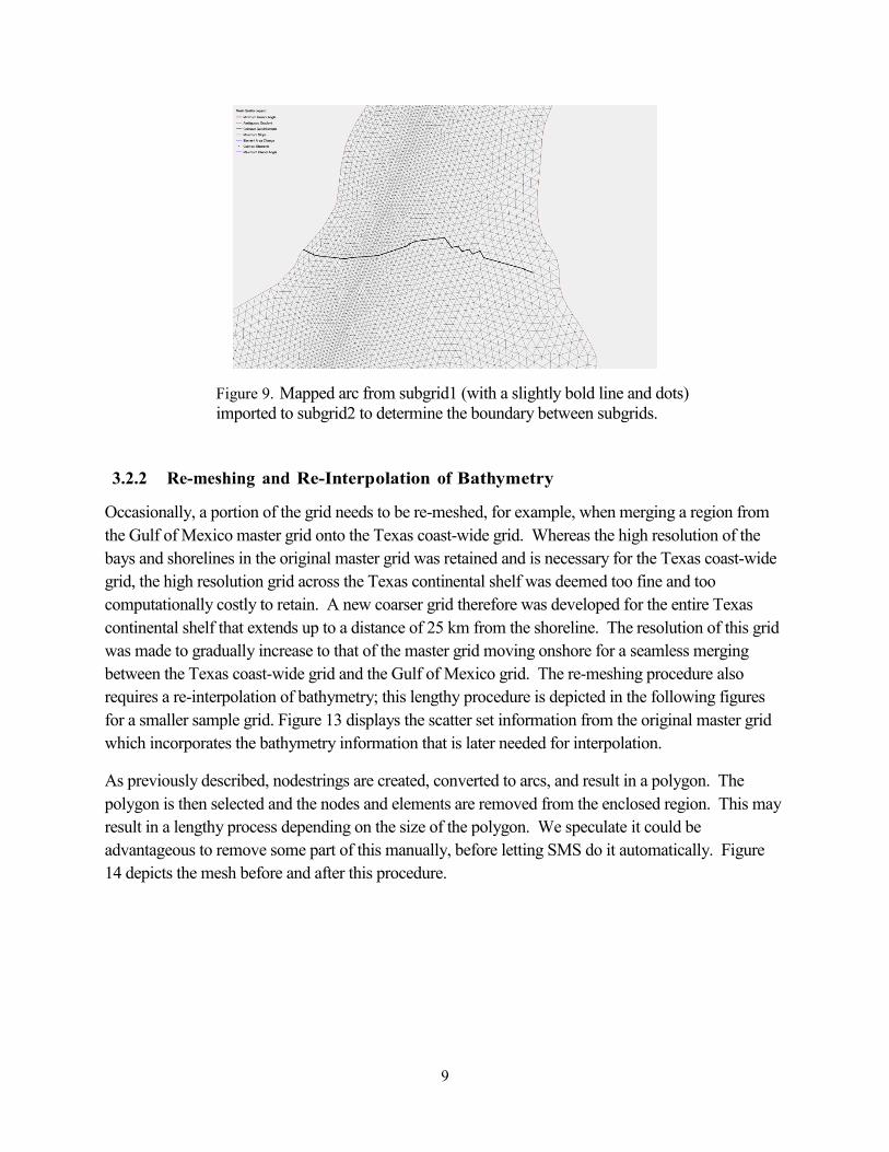
Figure 9. Mapped arc from subgrid1 (with a slightly bold line and dots) imported to subgrid2 to determine the boundary between subgrids.

3.2.2 Re-meshing and Re-Interpolation of Bathymetry

Occasionally, a portion of the grid needs to be re-meshed, for example, when merging a region from the Gulf of Mexico master grid onto the Texas coast-wide grid. Whereas the high resolution of the bays and shorelines in the original master grid was retained and is necessary for the Texas coast-wide grid, the high resolution grid across the Texas continental shelf was deemed too fine and too computationally costly to retain. A new coarser grid therefore was developed for the entire Texas continental shelf that extends up to a distance of 25 km from the shoreline. The resolution of this grid was made to gradually increase to that of the master grid moving onshore for a seamless merging between the Texas coast-wide grid and the Gulf of Mexico grid. The re-meshing procedure also requires a re-interpolation of bathymetry; this lengthy procedure is depicted in the following figures for a smaller sample grid. Figure 13 displays the scatter set information from the original master grid which incorporates the bathymetry information that is later needed for interpolation.

As previously described, nodestrings are created, converted to arcs, and result in a polygon. The polygon is then selected and the nodes and elements are removed from the enclosed region. This may result in a lengthy process depending on the size of the polygon. We speculate it could be advantageous to remove some part of this manually, before letting SMS do it automatically. Figure 14 depicts the mesh before and after this procedure.

10

Figure 10. Grids with overlapped regions removed

Figure 11. Grid with unsuccessful merged regions from grid 1 and grid 2 The next step involves breaking off the polygon arcs, specifying the vertices distribution, and interpolating the bathymetry. The resulting modified grid with a new meshed area is displayed in Figure 15. Re-meshing and re-interpolation is an iterative process and may have to be repeated several times before a proper mesh can be generated. Note the resulting modified grid in Figure 15 is not sufficiently accurate and would need to be re-meshed.

3.3 Conclusion of grid construction As a final step, boundary conditions are assigned; all of the islands, streams, and other land areas are enclosed by nodestrings. This is again a lengthy process due to the existence of overlapping nodestrings from previous modifications of the mesh and the identification and correction of faulty nodes that are generated during the re-meshing process. Finally, an overall grid quality check is conducted. This is an iterative process by which one must visually and manually modify the grid to obtain a high resolution, accurate finite-element mesh. It is particularly useful for CHG and TWDB personnel to collaborate during this process, so that important geophysical and

11

topographical surfaces are incorporated. Hence, a collaborative environment between TWDB and CHG personnel remains integrally important to the success of this project.

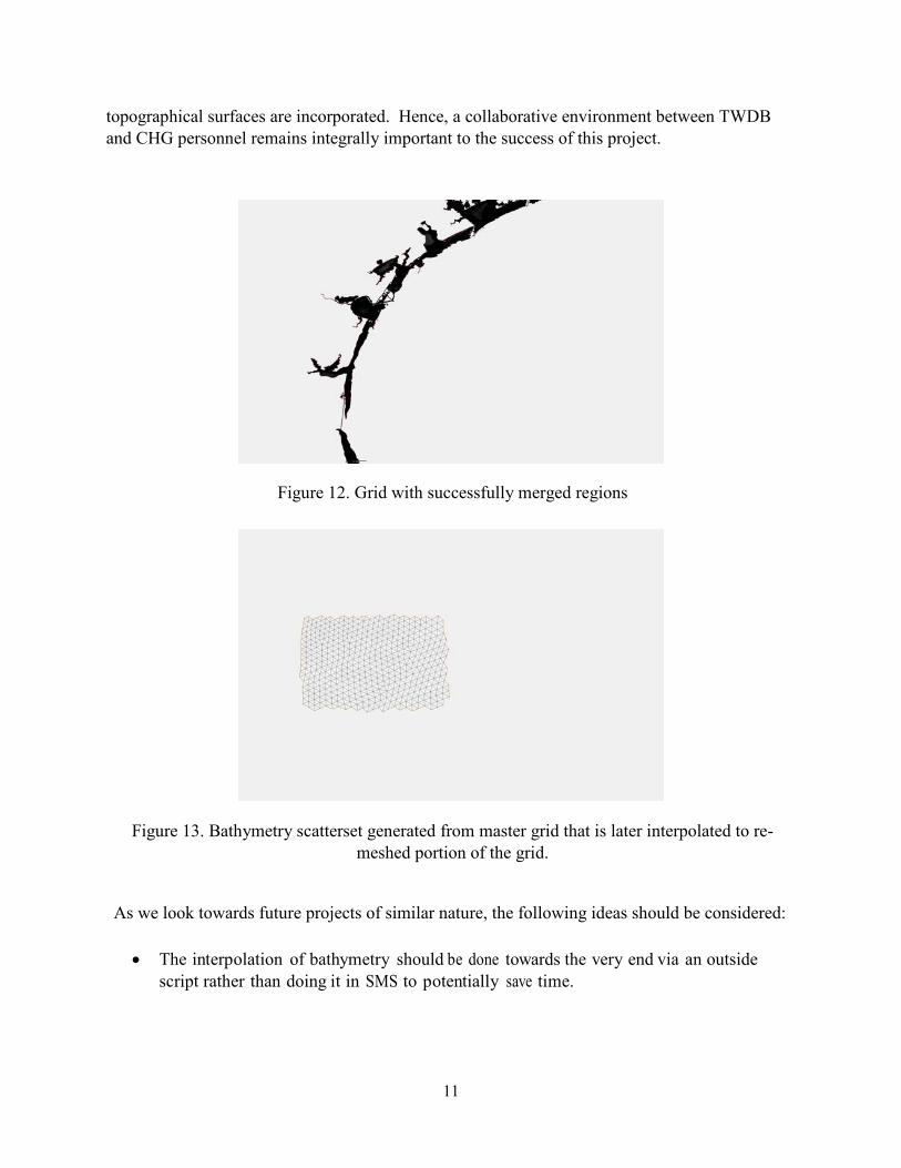
Figure 12. Grid with successfully merged regions

Figure 13. Bathymetry scatterset generated from master grid that is later interpolated to re-meshed portion of the grid.

As we look towards future projects of similar nature, the following ideas should be considered:

• The interpolation of bathymetry should be done towards the very end via an outside script rather than doing it in SMS to potentially save time.

12

• The map files on the TNRIS website [6] are very large and sometimes result in huge lags while working with them. The use of Google Images might save a considerable amount of time with a minimal loss of accuracy.

• Use of different software than SMS for modeling purposes. Our team is looking at other grid development/modification softwares that might be faster and more user friendly than SMS.

Figure 14. Grids before and after region removed enclosed by polygon

Figure 15. Grid with unsuccessful re-meshed area

13

4 Verification and Validation The Gulf of Mexico master grid, from which the Texas coast-wide grid was developed, has been extensively tested and used in storm surge simulations. In addition, the portions of grid that were extracted and merged into the coast-wide grid are quality checked in SMS. The grid was evaluated for abrupt area changes in adjacent elements, inappropriate element shape/size, and connecting elements which are relevant to most hydrodynamic models (www.xmswiki.com/xms/SMS:Mesh_Quality). However since the master grid was extensively tested in previous applications, the number of violating elements was insignificant with most occurring in the merging zones between the different bay subgrids. These elements were fixed manually so that there was no abrupt area changes in neighboring elements, elements were not too thin, etc. After this preliminary check, two SELFE model test cases were set up for Corpus Christi Bay and for a Texas coast-wide simulation. The Corpus Christi Bay test case was set up using boundary conditions and model parameters consistent with previously validated SELFE model (http://www.twdb.texas.gov/publications/reports/contracted_reports/doc/0904830892.pdf) whereas the Texas coast-wide case was set up with constant boundary conditions with the goal of testing the grid quality and boundary condition input consistency as an initial test case. After all pertinent input files were prepared, each model was run in the pre-processing mode to check the geometric quality of the grid and that the input files were consistent with the grid. Both models passed this initial preprocessing check. Due to the complexity of the model verification and validation process, the validation portion of the Corpus Christi and Texas coast-wide models is ongoing by TWDB staff. In particular, the testing of these grids in the finite-element model SELFE is an active area of research. Consider the following simulation: the SELFE code is compiled for the Texas Advanced Computing Center (TACC) Lonestar environment; the preprocessor, which creates pertinent supporting files for the model such as “centers.bp”, is successfully completed. However, the testing and verification process is tedious due to the necessity of continuing to modify the mesh “hgrid.gr3”. At the beginning portion of the computation, the program identifies problem areas of the grid via the warning error:

application called MPIAbort(comm=0x84000004, 0) - process 20 3: ABORT: Dry bnd side: 0.000000000000000E+000 14 24 105385

When this occurs, the grid must be modified manually, given the nodal id number 105196 to a positive or non-dry boundary condition. Because SELFE does not identify all nodes at the same time, this remains an iterative process. Indeed there is no obvious technique at this point for identifying these nodes other than by submission of a full parallel simulation.

In a separate study to model the La Quinta Channel in Corpus Christi Bay, a model grid was developed from the Corpus Christi, Mission-Aransas, and Upper Laguna Madre portions of the Texas coast-wide grid. The above mentioned issues were resolved by the selection of a proper

14

computational time-step through an iterative process. Visualization of the velocity fields has shown the model grid to be stable, though validation of the model to field observations is ongoing. 5 Conclusions A series of high-resolution subgrids and a high resolution coast-wide grid for Texas estuaries have been developed by extracting and modifying the successfully implemented Gulf of Mexico master grid. The Texas coast-wide grid incorporates all bays, estuaries, waterways, and channels along the Texas coast with sufficient resolution to model the primary hydrodynamic interactions among the different systems. TWDB staff recently extracted a regional grid from the Texas coast-wide grid in order to model hydrodynamic conditions in the La Quinta Channel of Corpus Christi Bay. They found the model grid to be quality assured and stable, but continue the process of evaluating the scalability and efficiency of model runs. Given the performance of the La Quinta grid and the noted consistency in mesh quality across all bays, as identified by SMS and SELFE, it is expected that all areas of the coast-wide grid will perform similarly when extracted for use in other models. TWDB anticipates extracting select portions of the Texas coast-wide grid as necessary to develop other bay- or region-specific hydrodynamic models and does not anticipate developing a coast-wide model in the near-term. However, evaluating the stability, scaling, and efficiency of applying new grids to three-dimensional models remains an area of active research.

6 References

[1] C. Dawson, J. Proft, V. Aizinger, UTBEST3D hydrodynamic model verification of Corpus Christi Bay, TWDB report September 2011.

[2] A. Fortunato, N. Bruneau, A. Azevedo, M. Araujo, A. Oliveira, Automatic improvement

of unstructured grids for coastal simulations, Journal of Coastal Research, Special Issue 64, 2011.

[3] H. Roberts, Grid generation methods for high resolution finite element models used for

hurricane storm surge prediction, Masters Thesis, Notre Dame University, 2004. [4] Aquaveo Water Modeling Solutions, http://www.ems-i.com/SMS/SMS overview/sms

overview.html

[5] A. Kennedy, U. Gravois, B. Zachry, J. Westerink, M. Hope, J. Dietrich, M. Powell, A. Cox, R. Luettich Jr, R. Dean, Origin of the Hurricane Ike Forerunner Surge, Geophysical Research Letters, 38, 2011.

[6] Texas Natural Resources Information System, http://www.tnris.org/get-data

15

[7] Y. J. Zhang, Technical support – Inter-model comparison for Corpus Christi Bay Testbed,

TWDB report, May 2010.

16

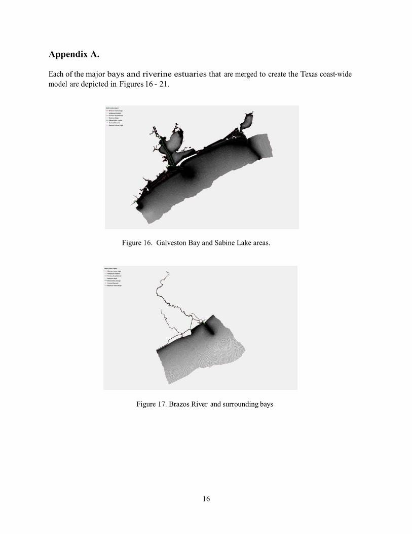
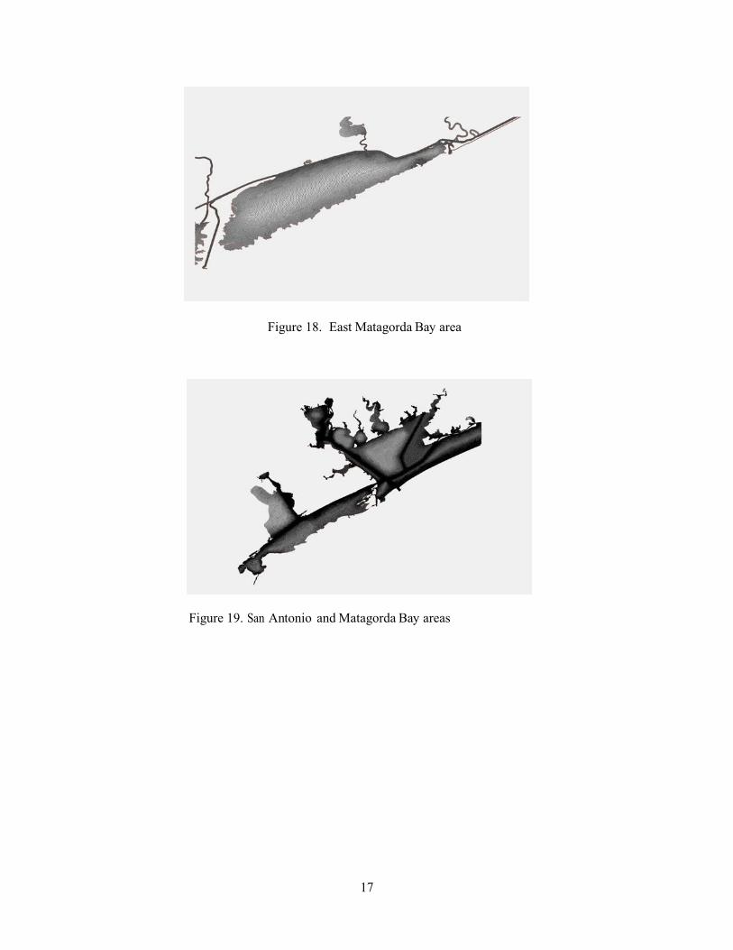
Appendix A. Each of the major bays and riverine estuaries that are merged to create the Texas coast-wide model are depicted in Figures 16 - 21.

Figure 16. Galveston Bay and Sabine Lake areas.

Figure 17. Brazos River and surrounding bays

17

Figure 18. East Matagorda Bay area

Figure 19. San Antonio and Matagorda Bay areas

18

Figure 20. Corpus Christi, Aransas and Upper Laguna Madre Bay Areas

Figure 21. Upper and Lower Laguna Madre area