CNN-RNN: A Unified Framework for Multi-label Image Classification

Jiang Wang1 Yi Yang1 Junhua Mao2 Zhiheng Huang3∗ Chang Huang4∗ Wei Xu1

1Baidu Research 2University of California at Los Angles 3Facebook Speech 4 Horizon Robotics

Abstract

While deep convolutional neural networks (CNNs) have

shown a great success in single-label image classification,

it is important to note that real world images generally con-

tain multiple labels, which could correspond to different

objects, scenes, actions and attributes in an image. Tradi-

tional approaches to multi-label image classification learn

independent classifiers for each category and employ rank-

ing or thresholding on the classification results. These tech-

niques, although working well, fail to explicitly exploit the

label dependencies in an image. In this paper, we utilize

recurrent neural networks (RNNs) to address this problem.

Combined with CNNs, the proposed CNN-RNN framework

learns a joint image-label embedding to characterize the

semantic label dependency as well as the image-label rel-

evance, and it can be trained end-to-end from scratch to

integrate both information in a unified framework. Exper-

imental results on public benchmark datasets demonstrate

that the proposed architecture achieves better performance

than the state-of-the-art multi-label classification models.

1. Introduction

Every real-world image can be annotated with multiple

labels, because an image normally abounds with rich se-

mantic information, such as objects, parts, scenes, actions,

and their interactions or attributes. Modeling the rich se-

mantic information and their dependencies is essential for

image understanding. As a result, multi-label classification

task is receiving increasing attention [12, 9, 24, 36]. In-

spired by the great success from deep convolutional neural

networks in single-label image classification in the past few

years [17, 29, 32], which demonstrates the effectiveness of

end-to-end frameworks, we explore to learn a unified frame-

work for multi-label image classification.

A common approach that extends CNNs to multi-label

classification is to transform it into multiple single-label

classification problems, which can be trained with the rank-

ing loss [9] or the cross-entropy loss [12]. However, when

treating labels independently, these methods fail to model

∗This work was done when the authors are at Baidu Research.

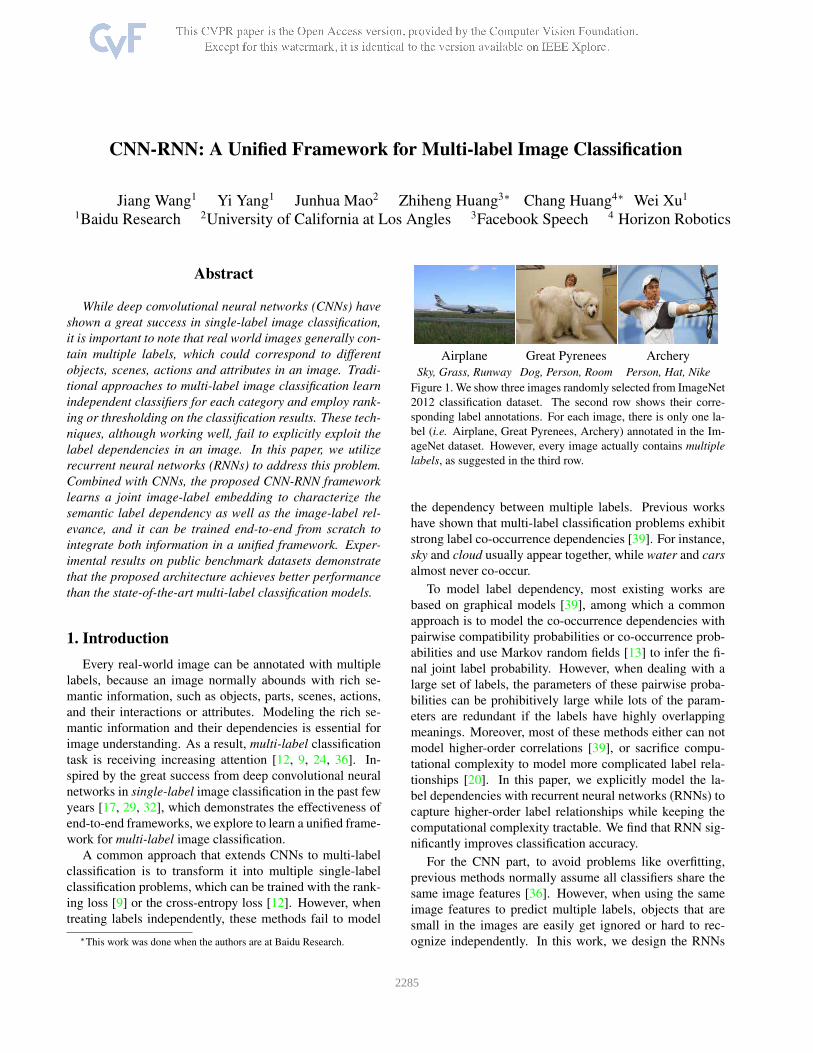
Airplane Great Pyrenees Archery

Sky, Grass, Runway Dog, Person, Room Person, Hat, Nike

Figure 1. We show three images randomly selected from ImageNet

2012 classification dataset. The second row shows their corre-

sponding label annotations. For each image, there is only one la-

bel (i.e. Airplane, Great Pyrenees, Archery) annotated in the Im-

ageNet dataset. However, every image actually contains multiple

labels, as suggested in the third row.

the dependency between multiple labels. Previous works

have shown that multi-label classification problems exhibit

strong label co-occurrence dependencies [39]. For instance,

sky and cloud usually appear together, while water and cars

almost never co-occur.

To model label dependency, most existing works are

based on graphical models [39], among which a common

approach is to model the co-occurrence dependencies with

pairwise compatibility probabilities or co-occurrence prob-

abilities and use Markov random fields [13] to infer the fi-

nal joint label probability. However, when dealing with a

large set of labels, the parameters of these pairwise proba-

bilities can be prohibitively large while lots of the param-

eters are redundant if the labels have highly overlapping

meanings. Moreover, most of these methods either can not

model higher-order correlations [39], or sacrifice compu-

tational complexity to model more complicated label rela-

tionships [20]. In this paper, we explicitly model the la-

bel dependencies with recurrent neural networks (RNNs) to

capture higher-order label relationships while keeping the

computational complexity tractable. We find that RNN sig-

nificantly improves classification accuracy.

For the CNN part, to avoid problems like overfitting,

previous methods normally assume all classifiers share the

same image features [36]. However, when using the same

image features to predict multiple labels, objects that are

small in the images are easily get ignored or hard to rec-

ognize independently. In this work, we design the RNNs

12285

framework to adapt the image features based on the pre-

vious prediction results, by encoding the attention models

implicitly in the CNN-RNN structure. The idea behind it

is to implicitly adapt the attentional area in images so the

CNNs can focus its attention on different regions of the im-

ages when predicting different labels. For example, when

predicting multiple labels for images in Figure 1, our model

will shift its attention to smaller ones (i.e. Runway, Person,

Hat) after recognizing the dominant object (i.e. Airplane,

Great Pyrenees, Archery). These small objects are hard to

recognize by itself, but can be easily inferred given enough

contexts.

Finally, many image labels have overlapping meanings.

For example, cat and kitten have almost the same meanings

and are often interchangeable. Not only does exploiting

the semantic redundancies reduce the computational cost, it

also improves the generalization ability because the labels

with duplicate semantics can get more training data.

The label semantic redundancy can be exploited by joint

image/label embedding, which can be learned via canoni-

cal correlation analysis [10], metric learning [19], or learn-

ing to rank methods [37]. The joint image/label embedding

maps each label or image to an embedding vector in a joint

low-dimensional Euclidean space such that the embeddings

of semantically similar labels are close to each other, and

the embedding of each image should be close to that of

its associated labels in the same space. The joint embed-

ding model can exploit label semantic redundancy because

it essentially shares classification parameters for semanti-

cally similar labels. However, the label co-occurrence de-

pendency is largely ignored in most of these models.

In this paper, we propose a unified CNN-RNN frame-

work for multi-label image classification, which effectively

learns both the semantic redundancy and the co-occurrence

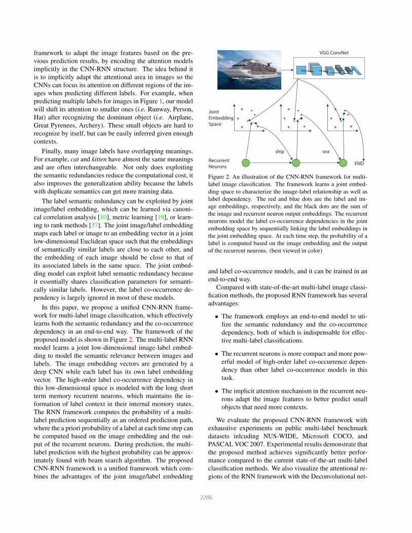
dependency in an end-to-end way. The framework of the

proposed model is shown in Figure 2. The multi-label RNN

model learns a joint low-dimensional image-label embed-

ding to model the semantic relevance between images and

labels. The image embedding vectors are generated by a

deep CNN while each label has its own label embedding

vector. The high-order label co-occurrence dependency in

this low-dimensional space is modeled with the long short

term memory recurrent neurons, which maintains the in-

formation of label context in their internal memory states.

The RNN framework computes the probability of a multi-

label prediction sequentially as an ordered prediction path,

where the a priori probability of a label at each time step can

be computed based on the image embedding and the out-

put of the recurrent neurons. During prediction, the multi-

label prediction with the highest probability can be approx-

imately found with beam search algorithm. The proposed

CNN-RNN framework is a unified framework which com-

bines the advantages of the joint image/label embedding

VGG ConvNet

Recurrent

Neurons

Joint

Embedding

Space

ship sea

END

Figure 2. An illustration of the CNN-RNN framework for multi-

label image classification. The framework learns a joint embed-

ding space to characterize the image-label relationship as well as

label dependency. The red and blue dots are the label and im-

age embeddings, respectively, and the black dots are the sum of

the image and recurrent neuron output embeddings. The recurrent

neurons model the label co-occurrence dependencies in the joint

embedding space by sequentially linking the label embeddings in

the joint embedding space. At each time step, the probability of a

label is computed based on the image embedding and the output

of the recurrent neurons. (best viewed in color)

and label co-occurrence models, and it can be trained in an

end-to-end way.

Compared with state-of-the-art multi-label image classi-

fication methods, the proposed RNN framework has several

advantages:

• The framework employs an end-to-end model to uti-

lize the semantic redundancy and the co-occurrence

dependency, both of which is indispensable for effec-

tive multi-label classifications.

• The recurrent neurons is more compact and more pow-

erful model of high-order label co-occurrence depen-

dency than other label co-occurrence models in this

task.

• The implicit attention mechanism in the recurrent neu-

rons adapt the image features to better predict small

objects that need more contexts.

We evaluate the proposed CNN-RNN framework with

exhaustive experiments on public multi-label benchmark

datasets inlcuding NUS-WIDE, Microsoft COCO, and

PASCAL VOC 2007. Experimental results demonstrate that

the proposed method achieves significantly better perfor-

mance compared to the current state-of-the-art multi-label

classification methods. We also visualize the attentional re-

gions of the RNN framework with the Deconvolutional net-

2286

works [40]. Interestingly, the visualization shows that the

RNN framework can focus on the corresponding image re-

gions when predicting different labels, which is very similar

to humans’ multi-label classification process.

2. Related Work

The progress of image classification is partly due to the

creation of large-scale hand-labeled datasets such as Ima-

geNet [5], and the development of deep convolutional neu-

ral networks [17]. Recent work that extends deep convolu-

tional neural networks to multi-label classification achieves

good results. Deep convolutional ranking [9] optimizes a

top-k ranking objective, which assigns smaller weights to

the loss if the positive label. Hypotheses-CNN-Pooling

[36] employs max pooling to aggregate the predictions

from multiple hypothesis region proposals. These methods

largely treat each label independently and ignore the corre-

lations between labels.

Multi-label classification can also be achieved by learn-

ing a joint image/label embedding. Multiview Canonical

Correlation Analysis [10] is a three-way canonical analy-

sis that maps the image, label, and the semantics into the

same latent space. WASABI [37] and DEVISE [7] learn

the joint embedding using the learning to rank framework

with WARP loss. Metric learning [19] learns a discrimi-

native metric to measure the image/label similarity. Matrix

completion [1] and bloom filter [3] can also be employed

as label encodings. These methods effectively exploit the

label semantic redundancy, but they fall short on modeling

the label co-occurrence dependency.

Various approaches have been proposed to exploit the la-

bel co-occurrence dependency for multi-label image classi-

fication. [28] learns a chain of binary classifiers, where each

classifier predicts whether the current label exists given the

input feature and the already predicted labels. The label

co-occurrence dependency can also be modeled by graphi-

cal models, such as Conditional Random Field [8], Depen-

dency Network [13], and co-occurrence matrix[39]. Label

augment model [20] augments the label set with common

label combinations. Most of these models only capture

pairwise label correlations and have high computation cost

when the number of labels is large. The low-dimensional

recurrent neurons in the proposed RNN model are more

computationally efficient representations for high-order la-

bel correlation.

RNN with LSTM can effectively model the long-term

temporal dependency in a sequence. It has been success-

fully applied in image captioning [25, 35], machine transla-

tion [31], speech recognition [11], language modeling [30],

and word embedding learning [18]. We demonstrate that

RNN with LSTM is also an effective model for label de-

pendency.

∏

∑

∏

input

gate

forget

gate

output

gate

update

term

∏

xt it ft ot

r(t)

o(t)

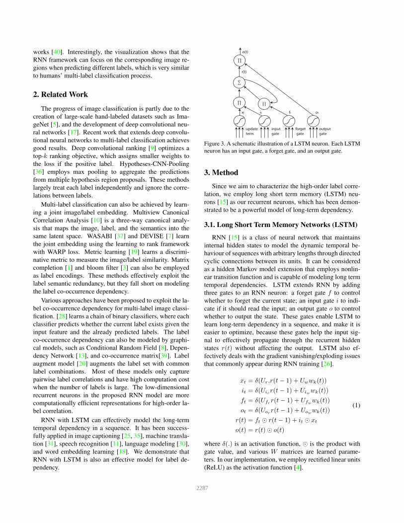
Figure 3. A schematic illustration of a LSTM neuron. Each LSTM

neuron has an input gate, a forget gate, and an output gate.

3. Method

Since we aim to characterize the high-order label corre-

lation, we employ long short term memory (LSTM) neu-

rons [15] as our recurrent neurons, which has been demon-

strated to be a powerful model of long-term dependency.

3.1. Long Short Term Memory Networks (LSTM)

RNN [15] is a class of neural network that maintains

internal hidden states to model the dynamic temporal be-

haviour of sequences with arbitrary lengths through directed

cyclic connections between its units. It can be considered

as a hidden Markov model extension that employs nonlin-

ear transition function and is capable of modeling long term

temporal dependencies. LSTM extends RNN by adding

three gates to an RNN neuron: a forget gate f to control

whether to forget the current state; an input gate i to indi-

cate if it should read the input; an output gate o to control

whether to output the state. These gates enable LSTM to

learn long-term dependency in a sequence, and make it is

easier to optimize, because these gates help the input sig-

nal to effectively propagate through the recurrent hidden

states r(t) without affecting the output. LSTM also ef-

fectively deals with the gradient vanishing/exploding issues

that commonly appear during RNN training [26].

xt = δ(Ur.r(t− 1) + Uwwk(t))

it = δ(Uirr(t− 1) + Uiwwk(t))

ft = δ(Ufrr(t− 1) + Ufwwk(t))

ot = δ(Uorr(t− 1) + Uowwk(t))

r(t) = ft ⊙ r(t− 1) + it ⊙ xt

o(t) = r(t)⊙ o(t)

(1)

where δ(.) is an activation function, ⊙ is the product with

gate value, and various W matrices are learned parame-

ters. In our implementation, we employ rectified linear units

(ReLU) as the activation function [4].

2287

3.2. Model

We propose a novel CNN-RNN framework for multi-

label classification problem. The illustration of the CNN-

RNN framework is shown in Fig. 4. It contains two parts:

The CNN part extracts semantic representations from im-

ages; the RNN part models image/label relationship and la-

bel dependency.

We decompose a multi-label prediction as an ordered

prediction path. For example, labels “zebra” and “elephant”

can be decomposed as either (“zebra”, “elephant”) or (“ele-

phant”, “zebra”). The probability of a prediction path can

be computed by the RNN network. The image, label, and

recurrent representations are projected to the same low-

dimensional space to model the image-text relationship as

well as the label redundancy. The RNN model is employed

as a compact yet powerful representation of the label co-

occurrence dependency in this space. It takes the embed-

ding of the predicted label at each time step and maintains a

hidden state to model the label co-occurrence information.

The a priori probability of a label given the previously pre-

dicted labels can be computed according to their dot prod-

ucts with the sum of the image and recurrent embeddings.

The probability of a prediction path can be obtained as the

product of the a-prior probability of each label given the

previous labels in the prediction path.

A label k is represented as a one-hot vector ek =[0, . . . 0, 1, 0, . . . , 0], which is 1 at the k-th location, and 0

elsewhere. The label embedding can be obtained by multi-

plying the one-hot vector with a label embedding matrix Ul.

The k-th row of Ul is the label embedding of the label k.

wk = Ul.ek. (2)

The dimension of wk is usually much smaller than the num-

ber of labels.

The recurrent layer takes the label embedding of the pre-

viously predicted label, and models the co-occurrence de-

pendencies in its hidden recurrent states by learning non-

linear functions:

o(t) = ho(r(t−1), wk(t)), r(t) = hr(r(t−1), wk(t)) (3)

where r(t) and o(t) are the hidden states and outputs of the

recurrent layer at the time step t, respectively, wk(t) is the

label embedding of the t-th label in the prediction path, and

ho(.), hr(.) are the non-linear RNN functions, which will

be described in details in Sec. 3.1.

The output of the recurrent layer and the image represen-

tation are projected into the same low-dimensional space as

the label embedding.

xt = h(Uxo o(t) + Ux

I I), (4)

where Uxo and Ux

I are the projection matrices for recurrent

layer output and image representation, respectively. The

Cu

rre

nt

La

be

l

La

be

l

Em

be

dd

ing

ek(t)

Re

curr

en

t

La

yer

wk(t)

Pro

ject

ion

La

yer

o(t)

Ima

ge

r(t)

ConvNetI

Pre

dic

tio

n

La

yer

Pre

dic

ted

La

be

l pro

ba

bil

ity

x(t)

UlUl

T

Figure 4. The architecture of the proposed RNN model for multi-

label classification. The convolutional neural network is employed

as the image representation, and the recurrent layer captures the

information of the previously predicted labels. The output label

probability is computed according to the image representation and

the output of the recurrent layer.

number of columns of Uxo and Ux

I are the same as the la-

bel embedding matrix Ul. I is the convolutional neural net-

work image representation. We will show in Sec 4.5 that the

learned joint embedding effectively characterizes the rele-

vance of images and labels.

Finally, the label scores can be computed by multiplying

the transpose of Ul and xt to compute the distances between

xt and each label embedding.

s(t) = UTl xt. (5)

The predicted label probability can be computed using soft-

max normalization on the scores.

3.3. Inference

A prediction path is a sequence of labels

(l1, l2, l3, · · · , lN ), where the probability of each la-

bel lt can be computed with the information of the image I

and the previously predicted labels l1, · · · , lt−1. The RNN

model predicts multiple labels by finding the prediction

path that maximizes the a priori probability.

l1, · · · , lk = arg maxl1,··· ,lk

P (l1, · · · , lk|I)

= arg maxl1,··· ,lk

P (l1|I)× P (l2|I, l1)

· · ·P (lk|I, l1, · · · , lk−1)

. (6)

Since the probability P (lk|I, l1, · · · , lk−1) does not have

Markov property, there is no optimal polynomial algo-

rithm to find the optimal prediction path. We can em-

ploy the greedy approximation, which predicts label lt =argmaxlt P (lt|I, l1, · · · , lt−1) at time step t and fix the la-

bel prediction lt at later predictions. However, the greedy

algorithm is problematic because if the first predicted label

is wrong, it is very likely that the whole sequence cannot

2288

Cat

Dog

Person

END

Car

Cat

Dog

Person

END

Car

Cat

Dog

Person

END

Car

Cat

Dog

Person

END

Car

Cat

Dog

Person

END

Car

Cat

Dog

Person

END

Car

Figure 5. An example of the beam search algorithm with beam

size N = 2. The beam search algorithm finds the best N paths

with the highest probability, by keeping a set of intermediate paths

at each time step and iteratively adding labels these intermediate

paths.

be correctly predicted. Thus, we employ the beam search

algorithm to find the top-ranked prediction path.

An example of the beam search algorithm can be found

in Figure 5. Instead of greedily predicting the most proba-

ble label, the beam search algorithm finds the top-N most

probable prediction paths as intermediate paths S(t) at each

time step t.

S(t) = {P1(t), P2(t), · · · , PN (t)} (7)

At time step t + 1, we add N most probable labels to each

intermediate path Pi(t) to get a total of N ×N paths. The

N prediction paths with highest probability among these

paths constitute the intermediate paths for time step t + 1.

The prediction paths ending with the END sign are added to

the candidate path set C. The termination condition of the

beam search is that the probability of the current intermedi-

ate paths is smaller than that of all the candidate paths. It

indicates that we cannot find any more candidate paths with

greater probability.

3.4. Training

Learning CNN-RNN models can be achieved by us-

ing the cross-entropy loss on the softmax normalization

of score softmax(s(t)) and employing back-propagation

through time algorithm. In order to avoid the gradient van-

ishing/exploding issues, we apply the rmsprop optimization

algorithm [33]. Although it is possible to fine-tune the con-

volutional neural network in our architecture, we keep the

convolutional neural network unchanged in our implemen-

tation for simplicity.

One important issue of training multi-label CNN-RNN

models is to determine the orders of the labels. In the ex-

periments of this paper, the label orders during training are

determined according to their occurrence frequencies in the

training data. More frequent labels appear earlier than the

less frequent ones, which corresponds to the intuition that

easier objects should be predicted first to help predict more

difficult objects. We explored learning label orders by iter-

atively finding the easiest prediction ordering and order en-

sembles as proposed in [28] or simply using fixed random

order, but they do not have notable effects on the perfor-

mance. We also attempted to randomly permute the label

orders in each mini-batch, but it makes the training very

difficult to converge.

4. Experiments

In our experiments, the CNN module uses the 16 lay-

ers VGG network [29] pretrained on ImageNet 2012 clas-

sification challenge dataset [5] using Caffe deep learning

framework [16]. The dimensions of the label embedding

and of LSTM RNN layer are 64 and 512, respectively. We

employ weight decay rate 0.0001, momentum rate 0.9, and

dropout [4] rate 0.5 for all the projection layers.

We evaluate the proposed method on three benchmark

multi-label classification datasets: NUS-WIDE, Microsoft

COCO, and VOC PASCAL 2007 datasets. The evaluation

demonstrates that the proposed method achieves superior

performance to state-of-the-art methods. We also quali-

tatively show that the proposed method learns a joint la-

bel/image embedding and it focuses its attention in different

image regions during the sequential prediction.

4.1. Evaluation Metric

The precision and recall of the generated labels are em-

ployed as evaluation metrics. For each image, we generate

k1 highest ranked labels and compare the generated labels

to the ground truth labels. The precision is the number of

correctly annotated labels divided by the number of gener-

ated labels; the recall is the number of correctly annotated

labels divided by the number of ground-truth labels.

We also compute the per-class and overall precision (C-

P and O-P) and recall scores (C-R and O-R), where the av-

erage is taken over all classes and all testing examples, re-

spectively. The F1 (C-F1 and O-F1) score is the geometrical

average of the precision and recall scores. We also compute

the mean average precision (MAP)@N measure [34].

4.2. NUS­WIDE

NUS-WIDE dataset [2] is a web image dataset that con-

tains 269,648 images and 5018 tags from Flickr. There are a

total of 1000 tags after removing noisy and rare tags. These

images are further manually annotated into 81 concepts by

1For RNN model, we set the minimum prediction length during beam

search to ensure that at least k labels are predicted.

2289

Tags80: clouds, sun, sunset

Tags1k: blue, clouds, sun, sunset,

light, orange, photographer

Prediction 80: clouds, sky, sun, sunset

Prediction 1k: nature, sky, blue, clouds,

red, sunset , yellow, sun, beatiful,

sunrise, cloud

Tags: car, person, luggage, backpack,

umbrella, cup, truck

Predictions: person, car, truck,

backpack

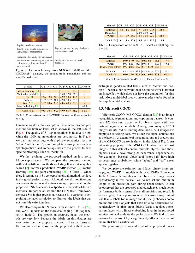
Figure 6. One example image from NUS-WIDE (left) and MS-

COCO(right) datasets, the ground-truth annotations and our

model’s predictions.

Method C-P P-R C-F1 O-P O-R O-F1 MAP@10

Metric Learning [19] - - - - - 21.3 -

Multi-edge graph [23] - - - 35.0 37.0 36.0 -

KNN [2] 32.6 19.3 24.3 42.9 53.4 47.6 -

Softmax 31.7 31.2 31.4 47.8 59.5 53.0 -

WARP [9] 31.7 35.6 33.5 48.6 60.5 53.9 -

Joint Embedding [38] - - - - - - 40.3

CNN-RNN 40.5 30.4 34.7 49.9 61.7 55.2 56.1

Table 1. Comparisons on NUS-WIDE Dataset on 81 concepts for

k = 3.

human annotators. An example of the annotations and pre-

dictions for both of label set is shown in the left side of

Fig. 6. The quality of 81-tag annotations is relatively high,

while the 1000-tag annotations are very noisy. In Fig. 6,

we can find some tags with duplicate semantics, such as

“cloud” and “clouds”, some completely wrong tags, such as

“photographer”, and some tags that are too general to have

specific meanings, such as “beautiful”.

We first evaluate the proposed method on less noisy

81 concepts labels. We compare the proposed method

with state-of-the-art methods including K nearest neighbor

search [2], softmax prediction, WARP method [9], metric

learning [19], and joint embedding [38] in Table 1. Since

there is less noise in 81 concepts labels, all methods achieve

fairly good performance. Although we do not fine-tune

our convolutional neural network image representation, the

proposed RNN framework outperforms the state-of-the-art

methods. In particular, we find the CNN-RNN framework

achieves 8% higher precision, because it is capable of ex-

ploiting the label correlation to filter out the labels that can

not possibly exist together.

We also compare RNN model with softmax, DSLR [22],

and WARP models on the more challenging 1000-tag label

set in Table 2. The prediction accuracy of all the meth-

ods are very low, because the labels on this dataset are

very noisy, but the proposed method still outperforms all

the baseline methods. We find the proposed method cannot

Method C-P P-R C-F1 O-P O-R O-F1 MAP@10

Softmax 14.2 18.6 16.1 17.1 28.8 21.5 24.3

DLSR [22] - - - 20.0 25.0 22.4 -

WARP 14.5 15.9 15.2 18.3 30.8 22.9 24.8

CNN-RNN 19.2 15.3 17.1 18.5 31.2 23.3 26.6

Table 2. Comparisons on NUS-WIDE Dataset on 1000 tags for

k = 10.

Method C-P P-R C-F1 O-P O-R O-F1 MAP@10

Softmax 59.0 57.0 58.0 60.2 62.1 61.1 47.4

WARP 59.3 52.5 55.7 59.8 61.4 60.7 49.2

Binary cross-entropy 59.3 58.6 58.9 61.7 65.0 63.3 -

No RNN 65.3 54.5 59.3 68.5 61.3 65.7 57.2

CNN-RNN 66.0 55.6 60.4 69.2 66.4 67.8 61.2

Table 3. Comparisons on MS-COCO Dataset for k = 3.

distinguish gender-related labels such as “actor” and “ac-

tress”, because our convolutional neural network is trained

on ImageNet, which does not have the annotation for this

task. More multi-label prediction examples can be found in

the supplemental materials.

4.3. Microsoft COCO

Microsoft COCO (MS-COCO) dataset [21] is an image

recognition, segmentation, and captioning dataset. It con-

tains 123 thousand images of 80 objects types with per-

instance segmentation labels. Among those images, 82783

images are utilized as training data, and 40504 images are

employed as testing data. We utilize the object annotations

as the labels. An example of the annotations and predictions

of the MS-COCO dataset is shown in the right of Fig. 6. An

interesting property of the MS-COCO dataset is that most

images in this dataset contain multiple objects, and these

objects usually have strong co-occurrence dependencies.

For example, “baseball glove” and “sport ball” have high

co-occurrence probability, while “zebra” and “cat” never

appear together.

We compare the softmax, multi-label binary cross en-

tropy, and WARP [9] models with the CNN-RNN model in

Table 3. Since the number of the objects per image varies

considerably in this dataset, we do not set the minimum

length of the prediction path during beam search. It can

be observed that the proposed method achieves much better

performance both in terms of overall precision and recall. It

has a slightly lower per-class recall because it may output

less than k labels for an image and it usually chooses not to

predict the small objects that have little co-occurrence de-

pendencies with other larger objects. We also replace the re-

current layer with a linear embedding layer in the proposed

architecture and evaluate the performance. We find that re-

moving the recurrent layer significantly affects the recall of

the multi-label classification.

The per-class precision and recall of the proposed frame-

2290

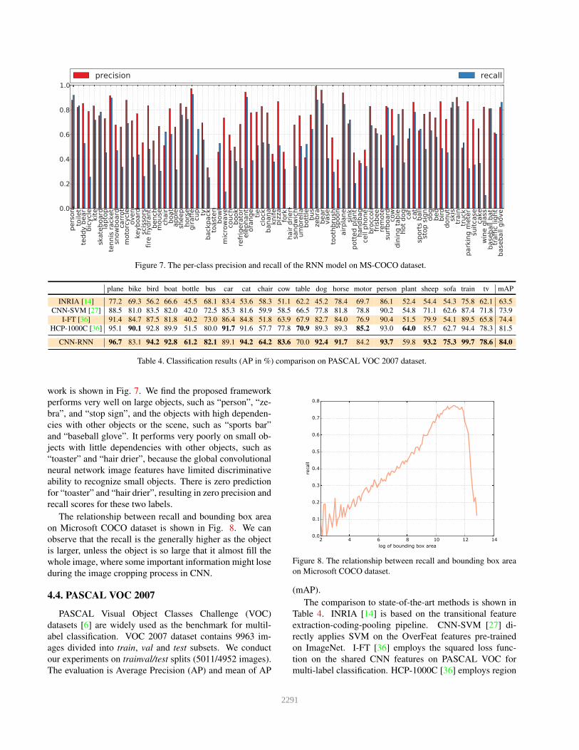
Figure 7. The per-class precision and recall of the RNN model on MS-COCO dataset.

plane bike bird boat bottle bus car cat chair cow table dog horse motor person plant sheep sofa train tv mAP

INRIA [14] 77.2 69.3 56.2 66.6 45.5 68.1 83.4 53.6 58.3 51.1 62.2 45.2 78.4 69.7 86.1 52.4 54.4 54.3 75.8 62.1 63.5

CNN-SVM [27] 88.5 81.0 83.5 82.0 42.0 72.5 85.3 81.6 59.9 58.5 66.5 77.8 81.8 78.8 90.2 54.8 71.1 62.6 87.4 71.8 73.9

I-FT [36] 91.4 84.7 87.5 81.8 40.2 73.0 86.4 84.8 51.8 63.9 67.9 82.7 84.0 76.9 90.4 51.5 79.9 54.1 89.5 65.8 74.4

HCP-1000C [36] 95.1 90.1 92.8 89.9 51.5 80.0 91.7 91.6 57.7 77.8 70.9 89.3 89.3 85.2 93.0 64.0 85.7 62.7 94.4 78.3 81.5

CNN-RNN 96.7 83.1 94.2 92.8 61.2 82.1 89.1 94.2 64.2 83.6 70.0 92.4 91.7 84.2 93.7 59.8 93.2 75.3 99.7 78.6 84.0

Table 4. Classification results (AP in %) comparison on PASCAL VOC 2007 dataset.

work is shown in Fig. 7. We find the proposed framework

performs very well on large objects, such as “person”, “ze-

bra”, and “stop sign”, and the objects with high dependen-

cies with other objects or the scene, such as “sports bar”

and “baseball glove”. It performs very poorly on small ob-

jects with little dependencies with other objects, such as

“toaster” and “hair drier”, because the global convolutional

neural network image features have limited discriminative

ability to recognize small objects. There is zero prediction

for “toaster” and “hair drier”, resulting in zero precision and

recall scores for these two labels.

The relationship between recall and bounding box area

on Microsoft COCO dataset is shown in Fig. 8. We can

observe that the recall is the generally higher as the object

is larger, unless the object is so large that it almost fill the

whole image, where some important information might lose

during the image cropping process in CNN.

4.4. PASCAL VOC 2007

PASCAL Visual Object Classes Challenge (VOC)

datasets [6] are widely used as the benchmark for multil-

abel classification. VOC 2007 dataset contains 9963 im-

ages divided into train, val and test subsets. We conduct

our experiments on trainval/test splits (5011/4952 images).

The evaluation is Average Precision (AP) and mean of AP

2 4 6 8 10 12 14log of bounding box area

0.0

0.1

0.2

0.3

0.4

0.5

0.6

0.7

0.8

reca

ll

Figure 8. The relationship between recall and bounding box area

on Microsoft COCO dataset.

(mAP).

The comparison to state-of-the-art methods is shown in

Table 4. INRIA [14] is based on the transitional feature

extraction-coding-pooling pipeline. CNN-SVM [27] di-

rectly applies SVM on the OverFeat features pre-trained

on ImageNet. I-FT [36] employs the squared loss func-

tion on the shared CNN features on PASCAL VOC for

multi-label classification. HCP-1000C [36] employs region

2291

Label Nearest Neighbors

glacier arctic, norway, volcano, tundra, lakes

sky nature, blue, clouds, landscape, bravo

sunset sun, landscape, light, bravo, yellow

rail railway, track, locomotive, tracks, steam

cat dog, bear, bird, hair drier, toaster

cow horse, sheep, bear, zebra, elephant

Table 5. Nearest neighbors for label embeddings of 1k labels of

NUS-WIDE and MS-COCO datasets

hawk, eagle, fauna,

wind, bird

glacier, volcano, cli�,

arctic, lakes

portraits, costume,

female, asian, hat

portraits,people, street,

hospital, woman

landscape, mountain,

nature, mountains, bravobird, hwak, nature,

bravo, birds

Ima

ge

s

KNN

Classi-

�cation

Figure 9. Nearest neighbor labels and top classification predictions

by softmax model for three query images of 1000 label set on

NUS-WIDE dataset.

proposal information to fine-tune the CNN features pre-

trained on ImageNet 1000 dataset, and ac hives better per-

formance than the methods that do not exploit region infor-

mation. The proposed CNN-RNN method outperforms the

I-FT method by a large margin, and it also performs better

than HCP-1000C method, although the RNN method does

not take the region proposal information into account.

4.5. Label embedding

In addition to being able to generate multiple labels, the

CNN-RNN model also effectively learns a joint label/image

embedding. The nearest neighbors of the labels in the em-

bedding space for NUS-WIDE and MS-COCO, are shown

in Table 5. We can see that a label is highly semantically

related to its nearest-neighbor labels.

Fig. 9 shows the nearest neighbor labels for images on

NUS-WIDE 1000-tag dataset computed according to label

embedding wk and image embedding UxI I . In the joint em-

bedding space, an image and its nearest neighbor labels are

semantically relevant. Moreover, we find that compared to

the top-ranked labels predicted by classification model, the

nearest neighbor labels are usually more fine-grained. For

example, the nearest neighbor labels “hawk” and “glacier”

are more fine-grained than “bird” and “landscape”.

Original Image Initial Attention Attention after first word

Figure 10. The attentional visualization for the RNN multi-label

framework. This image has two ground-truth labels: “elephant”

and “zebra”. The bottom-left image shows the framework’s atten-

tion in the beginning, and the bottom-right image shows its atten-

tion after predicting “elephant”.

4.6. Attention Visualization

It is interesting to investigate how the CNN-RNN frame-

work’s attention changes when predicting different labels.

We visualize the attention of the RNN multi-label model

with Deconvolutional networks [40] in Fig. 10. Given an

input image, the attention of the RNN multilabel model at

each time step is the average of the synthesized image of

all the label nodes at the softmax layer using Deconvolu-

tional network. The ground truth labels of this image are

“elephant” and “zebra”. (Notice that the visualization of

attention does not utilize the ground truth labels) At the be-

ginning, the attention visualization shows that the model

looks over the whole image and predicts “elephant”. Af-

ter predicting “elephant”, the model shifts its attention to

the regions of zebra and predicts “zebra”. The visualization

shows that although the RNN framework does not learn an

explicit attentional model, it manages to steer its attention to

different image regions when classifying different objects.

5. Conclusion and Future Work

We propose a unified CNN-RNN framework for multi-

label image classification. The proposed framework com-

bines the advantages of the joint image/label embedding

and label co-occurrence models by employing CNN and

RNN to model the label co-occurrence dependency in a

joint image/label embedding space. Experimental results on

several benchmark datasets demonstrate that the proposed

approach achieves superior performance to the state-of-the-

art methods.

The attention visualization shows that the proposed

model can steer its attention to different image regions when

predicting different labels. However, predicting small ob-

jects is still challenging due to the limited discriminative-

ness of the global visual features. It is an interesting di-

rection to not only predict the labels, but also predict the

segmentation of the objects by constructing an explicit at-

tention model. We will investigate that in our future work.

2292

References

[1] R. S. Cabral, F. Torre, J. P. Costeira, and A. Bernardino.

Matrix completion for multi-label image classification. In

Advances in Neural Information Processing Systems, pages

190–198, 2011. 3

[2] T.-S. Chua, J. Tang, R. Hong, H. Li, Z. Luo, and Y. Zheng.

Nus-wide: a real-world web image database from national

university of singapore. In Proceedings of the ACM inter-

national conference on image and video retrieval, page 48.

ACM, 2009. 5, 6

[3] M. M. Cisse, N. Usunier, T. Artieres, and P. Gallinari. Ro-

bust bloom filters for large multilabel classification tasks. In

Advances in Neural Information Processing Systems, pages

1851–1859, 2013. 3

[4] G. E. Dahl, T. N. Sainath, and G. E. Hinton. Improving

deep neural networks for lvcsr using rectified linear units

and dropout. In Acoustics, Speech and Signal Processing

(ICASSP), 2013 IEEE International Conference on, pages

8609–8613. IEEE, 2013. 3, 5

[5] J. Deng, W. Dong, R. Socher, L.-J. Li, K. Li, and L. Fei-

Fei. Imagenet: A large-scale hierarchical image database.

In Computer Vision and Pattern Recognition, 2009. CVPR

2009. IEEE Conference on, pages 248–255. IEEE, 2009. 3,

5

[6] M. Everingham, L. Van Gool, C. K. Williams, J. Winn, and

A. Zisserman. The pascal visual object classes (voc) chal-

lenge. International journal of computer vision, 88(2):303–

338, 2010. 7

[7] A. Frome, G. S. Corrado, J. Shlens, S. Bengio, J. Dean,

T. Mikolov, et al. Devise: A deep visual-semantic embed-

ding model. In Advances in Neural Information Processing

Systems, pages 2121–2129, 2013. 3

[8] N. Ghamrawi and A. McCallum. Collective multi-label clas-

sification. In Proceedings of the 14th ACM international con-

ference on Information and knowledge management, pages

195–200. ACM, 2005. 3

[9] Y. Gong, Y. Jia, T. Leung, A. Toshev, and S. Ioffe. Deep

convolutional ranking for multilabel image annotation. arXiv

preprint arXiv:1312.4894, 2013. 1, 3, 6

[10] Y. Gong, Q. Ke, M. Isard, and S. Lazebnik. A multi-view

embedding space for modeling internet images, tags, and

their semantics. International journal of computer vision,

106(2):210–233, 2014. 2, 3

[11] A. Graves, A.-R. Mohamed, and G. Hinton. Speech recog-

nition with deep recurrent neural networks. In Acoustics,

Speech and Signal Processing (ICASSP), 2013 IEEE Inter-

national Conference on, pages 6645–6649. IEEE, 2013. 3

[12] M. Guillaumin, T. Mensink, J. Verbeek, and C. Schmid.

Tagprop: Discriminative metric learning in nearest neigh-

bor models for image auto-annotation. In Computer Vision,

2009 IEEE 12th International Conference on, pages 309–

316. IEEE, 2009. 1

[13] Y. Guo and S. Gu. Multi-label classification using con-

ditional dependency networks. In IJCAI Proceedings-

International Joint Conference on Artificial Intelligence, vol-

ume 22, page 1300, 2011. 1, 3

[14] H. Harzallah, F. Jurie, and C. Schmid. Combining efficient

object localization and image classification. In Computer

Vision, 2009 IEEE 12th International Conference on, pages

237–244. IEEE, 2009. 7

[15] S. Hochreiter and J. Schmidhuber. Long short-term memory.

Neural computation, 9(8):1735–1780, 1997. 3

[16] Y. Jia, E. Shelhamer, J. Donahue, S. Karayev, J. Long, R. Gir-

shick, S. Guadarrama, and T. Darrell. Caffe: Convolu-

tional architecture for fast feature embedding. arXiv preprint

arXiv:1408.5093, 2014. 5

[17] A. Krizhevsky, I. Sutskever, and G. E. Hinton. Imagenet

classification with deep convolutional neural networks. In

Advances in neural information processing systems, pages

1097–1105, 2012. 1, 3

[18] P. Le and W. Zuidema. Compositional distributional se-

mantics with long short term memory. arXiv preprint

arXiv:1503.02510, 2015. 3

[19] J. Li, X. Lin, X. Rui, Y. Rui, and D. Tao. A distributed ap-

proach toward discriminative distance metric learning. Neu-

ral Networks and Learning Systems, IEEE Transactions on,

2014. 2, 3, 6

[20] X. Li, F. Zhao, and Y. Guo. Multi-label image classification

with a probabilistic label enhancement model. UAI, 2014. 1,

3

[21] T.-Y. Lin, M. Maire, S. Belongie, J. Hays, P. Perona, D. Ra-

manan, P. Dollar, and C. L. Zitnick. Microsoft coco: Com-

mon objects in context. In Computer Vision–ECCV 2014,

pages 740–755. Springer, 2014. 6

[22] Z. Lin, G. Ding, M. Hu, Y. Lin, and S. S. Ge. Image tag com-

pletion via dual-view linear sparse reconstructions. Com-

puter Vision and Image Understanding, 124:42–60, 2014. 6

[23] D. Liu, S. Yan, Y. Rui, and H.-J. Zhang. Unified tag analysis

with multi-edge graph. In Proceedings of the international

conference on Multimedia, pages 25–34. ACM, 2010. 6

[24] A. Makadia, V. Pavlovic, and S. Kumar. A new baseline for

image annotation. In Computer Vision–ECCV 2008, pages

316–329. Springer, 2008. 1

[25] J. Mao, W. Xu, Y. Yang, J. Wang, and A. Yuille. Deep cap-

tioning with multimodal recurrent neural networks (m-rnn).

In ICLR, 2015. 3

[26] R. Pascanu, T. Mikolov, and Y. Bengio. On the diffi-

culty of training recurrent neural networks. arXiv preprint

arXiv:1211.5063, 2012. 3

[27] A. S. Razavian, H. Azizpour, J. Sullivan, and S. Carlsson.

Cnn features off-the-shelf: an astounding baseline for recog-

nition. In Computer Vision and Pattern Recognition Work-

shops (CVPRW), 2014 IEEE Conference on, pages 512–519.

IEEE, 2014. 7

[28] J. Read, B. Pfahringer, G. Holmes, and E. Frank. Classi-

fier chains for multi-label classification. Machine learning,

85(3):333–359, 2011. 3, 5

[29] K. Simonyan and A. Zisserman. Very deep convolutional

networks for large-scale image recognition. arXiv preprint

arXiv:1409.1556, 2014. 1, 5

[30] M. Sundermeyer, R. Schluter, and H. Ney. Lstm neural net-

works for language modeling. In INTERSPEECH, 2012. 3

2293

[31] I. Sutskever, O. Vinyals, and Q. V. Le. Sequence to sequence

learning with neural networks. In Advances in Neural Infor-

mation Processing Systems, pages 3104–3112, 2014. 3

[32] C. Szegedy, W. Liu, Y. Jia, P. Sermanet, S. Reed,

D. Anguelov, D. Erhan, V. Vanhoucke, and A. Rabi-

novich. Going deeper with convolutions. arXiv preprint

arXiv:1409.4842, 2014. 1

[33] T. Tieleman and G. Hinton. Lecture 6.5-rmsprop: Divide

the gradient by a running average of its recent magnitude.

COURSERA: Neural Networks for Machine Learning, 4,

2012. 5

[34] A. Turpin and F. Scholer. User performance versus preci-

sion measures for simple search tasks. In Proceedings of

the 29th annual international ACM SIGIR conference on Re-

search and development in information retrieval, pages 11–

18. ACM, 2006. 5

[35] O. Vinyals, A. Toshev, S. Bengio, and D. Erhan. Show

and tell: A neural image caption generator. arXiv preprint

arXiv:1411.4555, 2014. 3

[36] Y. Wei, W. Xia, J. Huang, B. Ni, J. Dong, Y. Zhao, and

S. Yan. Cnn: Single-label to multi-label. arXiv preprint

arXiv:1406.5726, 2014. 1, 3, 7

[37] J. Weston, S. Bengio, and N. Usunier. Wsabie: Scaling up

to large vocabulary image annotation. In IJCAI, volume 11,

pages 2764–2770, 2011. 2, 3

[38] F. Wu, X. Jiang, X. Li, S. Tang, W. Lu, Z. Zhang, and

Y. Zhuang. Cross-modal learning to rank via latent joint

representation. Image Processing, IEEE Transactions on,

24(5):1497–1509, 2015. 6

[39] X. Xue, W. Zhang, J. Zhang, B. Wu, J. Fan, and Y. Lu.

Correlative multi-label multi-instance image annotation. In

Computer Vision (ICCV), 2011 IEEE International Confer-

ence on, pages 651–658. IEEE, 2011. 1, 3

[40] M. D. Zeiler, D. Krishnan, G. W. Taylor, and R. Fergus.

Deconvolutional networks. In Computer Vision and Pat-

tern Recognition (CVPR), 2010 IEEE Conference on, pages

2528–2535. IEEE, 2010. 3, 8

2294