Deep RNN Framework for Visual Sequential Applications

Bo Pang∗ Kaiwen Zha∗ Hanwen Cao Chen Shi Cewu Lu†

Shanghai Jiao Tong University

pangbo, kevin zha, mbd chw, shichen, lucewu@sjtu.edu.cn

Abstract

Extracting temporal and representation features effi-

ciently plays a pivotal role in understanding visual se-

quence information. To deal with this, we propose a new

recurrent neural framework that can be stacked deep ef-

fectively. There are mainly two novel designs in our deep

RNN framework: one is a new RNN module called Context

Bridge Module (CBM) which splits the information flowing

along the sequence (temporal direction) and along depth

(spatial representation direction), making it easier to train

when building deep by balancing these two directions; the

other is the Overlap Coherence Training Scheme that re-

duces the training complexity for long visual sequential

tasks on account of the limitation of computing resources.

We provide empirical evidence to show that our deep

RNN framework is easy to optimize and can gain accu-

racy from the increased depth on several visual sequence

problems. On these tasks, we evaluate our deep RNN

framework with 15 layers, 7× than conventional RNN net-

works, but it is still easy to train. Our deep framework

achieves more than 11% relative improvements over shal-

low RNN models on Kinetics, UCF-101, and HMDB-51

for video classification. For auxiliary annotation, after re-

placing the shallow RNN part of Polygon-RNN with our

15-layer deep CBM, the performance improves by 14.7%.

For video future prediction, our deep RNN improves the

state-of-the-art shallow model’s performance by 2.4% on

PSNR and SSIM. The code and trained models are pub-

lished accompanied by this paper: https://github.

com/BoPang1996/Deep-RNN-Framework.

1. Introduction

With the advent of deep neural networks (DNN) in recent

years, a mass of vision tasks have made great progress [25,

53, 40, 36, 12] due to its superior representation capabil-

ity for high-dimensional data. On top of spatial represen-

∗Equal contribution.†Corresponding author. Cewu Lu is a member of Department of Com-

puter Science and Engineering, Shanghai Jiao Tong University, MoE Key

Lab of Artificial Intelligence, AI Institute, Shanghai Jiao Tong University.

tation, temporal features are valuable and crucial as well

when dealing with sequential inputs like videos, for which

recurrent neural networks (RNN) are designed. Taking all

above into consideration, we are intended to build a deep

RNN architecture that combines the merits of both RNN

and DNN to extract more powerful temporal and represen-

tation features from visual sequential inputs.

A straightforward way to build RNN deeper is to simply

stack multiple RNN layers. However, this method is en-

countered with two problems. For one thing, in this deep

RNN structure, there exist two information flows — repre-

sentation flow and temporal flow, along structural (spatial)

depth and temporal depth respectively, however, these two

flows are often entangled with each other, making it hard

for models to be co-adaptive to both of them. Many spe-

cific RNN structures like LSTM [16] and GRU [6] are de-

signed mainly to capture temporal information among long

sequences, yet there is no adaption that can effectively take

advantage of both the two flows. Therefore, simply stacking

these RNN modules will lead to higher training error and

heavier training consumption. For another, the limitation

of computing resources greatly influences the feasibility of

this method. Unlike deep CNN [33, 27, 28], deep RNN

needs to unfold as many times as the sequence length, re-

sulting in more significant expansion of memory and com-

putational complexity with the depth increasing, especially

for visual sequential inputs.

In this paper, we propose a new deep RNN architecture

including two principle techniques, namely, Context Bridge

Module (CBM) and Overlap Coherence Training Scheme.

In CBM, we design two computing units taking charge of

representation flow and temporal flow respectively, forcing

these two flows relatively independent of each other with

the aim of making them focus on representation and tempo-

ral information separately to ease the training process. After

these two units, a merge unit is utilized to synthesize them.

By adjusting the synthesizing method, we can balance the

dominant degree of each direction to better adapt to the re-

quirements of different tasks. Furthermore, to make repre-

sentation flow less influenced by temporal flow in the be-

ginning of training, we design the Temporal Dropout (TD)

423

to interdict the back-propagation of temporal information

across layers with a certain probability.

Besides, the proposed Overlap Coherence Training

Scheme aims at reducing the training cost of deep RNN.

Since the enormous training consumptions are largely due

to the long sequence, we introduce this training scheme that

randomly samples the long sequence with length l into sev-

eral overlapping short clips with length n and leverages the

overlaps as the communication bridge between the adjacent

clips to smooth the information propagation among clips. In

this way, we simplify the original Markov process of order

l into several ones of order n (n < l), which remarkably re-

duces the training complexity, and guarantees the temporal

information coherence among clips at the same time. Based

on overlaps, we design overlap coherence loss that forces

the detached clips to generate coherent results in order to

strengthen the consistency of temporal information, which

makes the model not a strict Markov process of order n, but

the complexity is still reduced.

We conduct comprehensive experiments on several tasks

to show the challenge of training deep RNN and evaluate

our proposed deep RNN framework. Results reveal that:

1) Deep RNN can enjoy accuracy gains from the greatly

increased depth, substantially better than the shallow net-

works. 2) Our CBM is more suitable for stacking deep com-

pared with other RNN structures like LSTM. 3) The overlap

coherence training scheme can effectively make many com-

puter vision problems with high-dimensional sequential in-

puts trainable on commonly-used computing devices.

We evaluate our framework on several visual sequence

tasks: action recognition and anticipation on UCF-101 [43],

HMDB-51 [26] and Kinetics [4], auxiliary annotation

(Polygon-RNN [5]) on Cityscapes [7], and video future pre-

diction on KTH [39]. For action recognition and anticipa-

tion tasks, our deep RNN framework achieves more than

11% relative improvements on all the datasets compared

with the shallow RNN models. For Polygon-RNN task, IoU

value improves by 14.7% on Cityscapes. For video future

prediction task, our deep RNN improves the performance

by 2.4% on PSNR [31] and SSIM [47] metrics.

2. Related Work

Methods for Visual Sequence Tasks Visual sequence

problems require models to extract hierarchical temporal

and representation features simultaneously. A slew of prior

arts have shed light on this tough problem: 1) An inchoate

approach is pooling the spatial representation features of ev-

ery item in the sequence, such as [23, 52] when dealing with

video classification and [46, 48] for action detection and lo-

calization. This approach can extract relative high-quality

spatial representation features but is very weak for tempo-

ral ones because it treats the sequence as a set and simply

combines the spatial features of the set as global temporal

features without considering order relations. 2) Then 3D

convolutional networks [22, 4] appear, which treat temporal

dimension equal to spatial dimension with its cubic convo-

lution kernel, while 3D convolutional networks need to con-

sume large amount of computing resources. 3) RNN [49, 8]

is designed to handle sequence problems, therefore it is

a natural idea to utilize RNN to encode temporal infor-

mation after obtaining spatial features, which is adopted

in [49, 8, 29, 34] for video classification, [8, 44] for video

description, [5, 1] for auxiliary annotation and [45, 50, 32]

for video future prediction. Whereas, currently used RNN

is shallow, which may limit its performance.

Exploration on Deep RNN In this paper, we focus on ex-

ploring appropriate deep structure for RNN model. There

are many previous works trying to address this problem.

In [35, 14], the authors evaluate several ways to extend

RNN deeper, and results show that stacked RNN has rel-

atively better performance and more importantly, stacking

method can synthesize temporal information in each layer

to extract hierarchical temporal-spatial features instead of

plain temporal, deep spatial features.

The learning computational complexity of deep RNN

significantly increases with the depth growing, thus in [38],

the authors propose a new RNN structure called LSTMP

to reduce the complexity. In [20, 21, 18, 14], researchers

prove that deep RNNs outperform associated shallow coun-

terparts that employ the same number of parameters. [20]

shows that each layer captures a different aspect of compo-

sitionality which reveals deep RNN’s ability to extract hi-

erarchical features, and a deep bidirectional RNN structure

is proposed in [21]. All these previous works prove the im-

portance of RNN depth in NLP and speech area, while for

high-dimensional inputs like videos in computer vision, it

is more challenging to tackle as we mentioned above. For

them, what we suppose to build is a deep RNN framework

which is easy to optimize even when inputs are large-scale

and can achieve promising improvements on performance

at the same time.

3. Deep RNN Framework

Deep model has exhibited superior performance in pro-

ducing powerful features, and we hope sequence modeling

can enjoy the deep representation as well. To this end, we

introduce our deep RNN framework in this section, which

contains two parts: context bridge module (CBM) designed

to effectively capture temporal and representation infor-

mation simultaneously, and the overlap coherence training

scheme to further simplify the training process.

3.1. Context Bridge Module

To model visual sequential inputs, we need to make sure

it can be trained efficiently when building deep. For this,

we design a non-shallow recurrent architecture to respec-

424

Upper Layer

Ci,t

Oi,t

Ci,t-1

Oi-1,t

T

ζ

R

Oi,t+1

Ci,t+1

Oi-1,t+1

T

ζ

RLater Seq

Figure 1. Structure of CBM. The blue lines represent representa-

tion flows, while red ones represent temporal flows. R, T and ζ de-

note representation unit, temporal unit and merge function respec-

tively. The dashed line (TD) means feeding forward is allowed but

back-propagation is forbidden with a certain probability.

tively capture temporal information from sequential inputs

(e.g. a sequence of frames in a video) and representation

information from each individual one (e.g. one frame of

the sequence). These two information flows are oriented to-

wards temporal depth and structural depth separately, and

we name them as temporal flow and representation flow.

Challenge The straight-forward design for deep RNN can

be a vertically stacked RNN architecture. However, in high-

dimensional visual tasks, parameters in RNN cell are hard

to be co-adaptive to two flows simultaneously, resulting in

ineffective and inefficient training. Extensive experiments

show this design is very hard to train. This is why we hardly

see stacked deep RNN in related literatures. In most cases,

people adopt shallow RNN which takes extracted CNN fea-

tures as inputs, though it is not an end-to-end pipeline.

Our Architecture Therefore, we go down to consider

how to capture these two branches of information flows as

independently as possible, through which the training pro-

cess can be much easier since the two relatively independent

branches can share the burden of learning and ease complex

co-adaptations. Specifically, for representation flow, we use

a computing unit (e.g. CNN structure) to extract features

of the individual input sample without recurrent operations,

while temporal flow adopts a RNN structure.

As shown in Fig. 1, in each cell, there is a “representa-

tion” unit R and a “temporal” unit T which act as a repre-

sentation feature extractor on individual input sample and

a temporal information encoder on the sequential inputs re-

spectively. Here R can be seen as a context bridge over the

temporal information. Intuitively, the representation infor-

mation flow would be encouraged to mainly propagate by

this bridge, since it doesn’t need to interwind with tempo-

ral information. Therefore, we call this module as Context

Bridge Module (CBM). By denoting oi−1,t as the input to

the module in ith layer at time stamp t, we have

1 0

1

1 1 1 1 1 1 1 1 1

Represen

tatio

n F

low

Temporal Flow

10-2

100

102

104

9 10 11 12 13 14 15 16 17 18

TD-rate=0.0

Seq_len=10 Model_depth=10

TD-rate=0.5 TD-rate=0.2 TD-rate=0.8 103

102

101

100 10-1

10-2

5 6 8 9 107

Seq_len=6 Model_depth=6

E(Nu

m_P

aths

)

Path Length Path Length

E(Nu

m_P

aths

)

Figure 2. Temporal flows adopting TD. Top: When setting the

TD rate to 1.0, all the colorized lines (red & purple) of temporal

flow cannot propagate back, while if only drop the red node out,

the gradients from red node’s temporal unit cannot flow backward

through the red lines. Bottom: Expectation numbers of back-

propagation paths with different lengths (paths from “0” to dif-

ferent “1” in Top) when adopting different TD rates. Note that the

back-propagation remains unchanged when setting TD rate to 0.0.

o′i,t = R(oi−1,t;ψi), (1)

where the representation unit R is designed as a conven-

tional CNN layer, namely ReLU(Conv(·)), and ψi is the

parameters of R in ith layer.

On the other hand, temporal flow is captured by T unit,

which is written as

ci,t = T (ci,t−1, oi−1,t;φi), (2)

where ci,t is the memory state in ith layer at time stamp t,

and φi is the parameters of T in ith layer. As a recurrent

architecture, T can be a Sigmoid(Conv(·)) (as simple as

the conventional RNN) or LSTM. In practice, we suggest

Sigmoid(Conv(·)) since it only consumes half of comput-

ing resources compared with LSTM cell, which greatly con-

tributes to building model deeper.

Finally, to fuse the information flows from the two units,

we introduce a merge unit,

oi,t = ζ(o′i,t, ci,t), (3)

where ζ is the merge function, and we adopt element-wise

production for ζ in our experiments.

Temporal Dropout To make training easier, we hope the

learning in representation flow direction less interwinds

with temporal flow in the beginning. After a desirable

neural representation is shaped, the learning in temporal

flow direction can be more efficient. To this end, we

introduce a Temporal Dropout (TD) scheme: forbidding

425

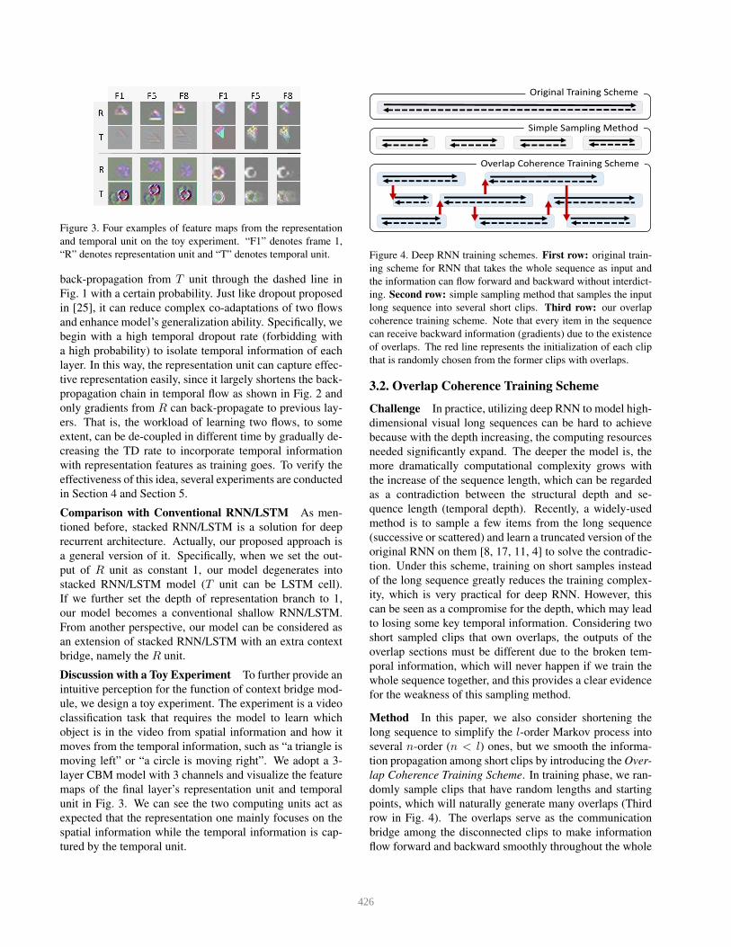
Figure 3. Four examples of feature maps from the representation

and temporal unit on the toy experiment. “F1” denotes frame 1,

“R” denotes representation unit and “T” denotes temporal unit.

back-propagation from T unit through the dashed line in

Fig. 1 with a certain probability. Just like dropout proposed

in [25], it can reduce complex co-adaptations of two flows

and enhance model’s generalization ability. Specifically, we

begin with a high temporal dropout rate (forbidding with

a high probability) to isolate temporal information of each

layer. In this way, the representation unit can capture effec-

tive representation easily, since it largely shortens the back-

propagation chain in temporal flow as shown in Fig. 2 and

only gradients from R can back-propagate to previous lay-

ers. That is, the workload of learning two flows, to some

extent, can be de-coupled in different time by gradually de-

creasing the TD rate to incorporate temporal information

with representation features as training goes. To verify the

effectiveness of this idea, several experiments are conducted

in Section 4 and Section 5.

Comparison with Conventional RNN/LSTM As men-

tioned before, stacked RNN/LSTM is a solution for deep

recurrent architecture. Actually, our proposed approach is

a general version of it. Specifically, when we set the out-

put of R unit as constant 1, our model degenerates into

stacked RNN/LSTM model (T unit can be LSTM cell).

If we further set the depth of representation branch to 1,

our model becomes a conventional shallow RNN/LSTM.

From another perspective, our model can be considered as

an extension of stacked RNN/LSTM with an extra context

bridge, namely the R unit.

Discussion with a Toy Experiment To further provide an

intuitive perception for the function of context bridge mod-

ule, we design a toy experiment. The experiment is a video

classification task that requires the model to learn which

object is in the video from spatial information and how it

moves from the temporal information, such as “a triangle is

moving left” or “a circle is moving right”. We adopt a 3-

layer CBM model with 3 channels and visualize the feature

maps of the final layer’s representation unit and temporal

unit in Fig. 3. We can see the two computing units act as

expected that the representation one mainly focuses on the

spatial information while the temporal information is cap-

tured by the temporal unit.

Original Training Scheme

Simple Sampling Method

Overlap Coherence Training Scheme

Figure 4. Deep RNN training schemes. First row: original train-

ing scheme for RNN that takes the whole sequence as input and

the information can flow forward and backward without interdict-

ing. Second row: simple sampling method that samples the input

long sequence into several short clips. Third row: our overlap

coherence training scheme. Note that every item in the sequence

can receive backward information (gradients) due to the existence

of overlaps. The red line represents the initialization of each clip

that is randomly chosen from the former clips with overlaps.

3.2. Overlap Coherence Training Scheme

Challenge In practice, utilizing deep RNN to model high-

dimensional visual long sequences can be hard to achieve

because with the depth increasing, the computing resources

needed significantly expand. The deeper the model is, the

more dramatically computational complexity grows with

the increase of the sequence length, which can be regarded

as a contradiction between the structural depth and se-

quence length (temporal depth). Recently, a widely-used

method is to sample a few items from the long sequence

(successive or scattered) and learn a truncated version of the

original RNN on them [8, 17, 11, 4] to solve the contradic-

tion. Under this scheme, training on short samples instead

of the long sequence greatly reduces the training complex-

ity, which is very practical for deep RNN. However, this

can be seen as a compromise for the depth, which may lead

to losing some key temporal information. Considering two

short sampled clips that own overlaps, the outputs of the

overlap sections must be different due to the broken tem-

poral information, which will never happen if we train the

whole sequence together, and this provides a clear evidence

for the weakness of this sampling method.

Method In this paper, we also consider shortening the

long sequence to simplify the l-order Markov process into

several n-order (n < l) ones, but we smooth the informa-

tion propagation among short clips by introducing the Over-

lap Coherence Training Scheme. In training phase, we ran-

domly sample clips that have random lengths and starting

points, which will naturally generate many overlaps (Third

row in Fig. 4). The overlaps serve as the communication

bridge among the disconnected clips to make information

flow forward and backward smoothly throughout the whole

426

…

…

…

Figure 5. “Cat & Dog” experiment. The input sequence is images

of cat and dog, and the label of each image represents the distance

from the cat image (padding with -1).

sequence. Therefore, we introduce a new loss called over-

lap coherence loss to force the outputs of overlaps from dif-

ferent clips to be as closed (coherent) as possible. Then, the

training objective function can be written as

N∑

i=1

Lr(si) + λ∑

(v,u)∈Ω

Ld(v, u), (4)

where si is the ith clip and Ω is the set of pairs which are the

outputs of overlap sections from different clips. Lr and Ld

denote the original loss for the specific task and our over-

lap coherence loss implemented by MSE loss respectively,

where λ is the hyper-parameter to adjust the weight of them.

Additionally, our training scheme exhibits several high-

lights in practice. Firstly, our random sampling mode serves

as a great data argumentation approach to enhance model’s

generalization ability. Secondly, the vanishing/exploding

gradient problem can be solved to some extent since the

scheme will shorten the sequence adequately to train easily.

Thirdly, the initial state of each clip is taken from other ear-

lier trained clips by picking up their hidden states at corre-

sponding time stamp, which further bridges the information

flow among clips to make it smoothly transfer throughout

the whole sequence. Furthermore, initialized clips can be

computed together in parallel, which can effectively reduce

the training time, especially when the overlap rate is high.

Moreover, to verify our training scheme can actually

transfer useful information flow throughout the whole se-

quence, we commit a toy experiment shown in Fig. 5. The

input sequence is a series of images, where there is only one

cat and the others are all dogs. We train a model with over-

lap coherence training scheme to learn how far the current

dog image is from the cat image appeared before. We find

that the model can correctly predict even if the cat image ap-

pearing 50 frames ago, where we set the clip length smaller

than 10. This is because temporal information of the image

sequence is successfully captured among clips due to our

overlap coherence training scheme.

4. Experimental Results

In this section, we evaluate our deep RNN framework

and compare it with conventional shallow RNN (we choose

the commonly used one: LSTM) on several sequence tasks

to exhibit the superiority of our deep RNN framework over

the shallow ones on high-dimensional inputs.

Figure 6. Shallow and deep RNN architecture. The shallow ver-

sion is implemented based on [8]. The deep one contains 15 RNN

layers and we add shortcuts along the depth, following [13]. Dif-

ferent from the shallow one, the RNN kernel is convolutional to

maintain the spatial features instead of linear kernel.

4.1. Video Action Recognition and Anticipation

We first evaluate our method with action recognition and

anticipation tasks [3, 30] on the UCF-101 dataset [43] and

HMDB-51 dataset [26] to compare our deep RNN with the

common shallow one with CNN backbones. Then we re-

move the backbones, evaluate the standalone deep RNN

model on Kinetics dataset [4] to compare it with several

excellent approaches, not merely the shallow RNN.

Implementation The frames in videos are resized with

its shorter side into 368 and a 224 × 224 crop is randomly

sampled from the frame or its horizontal flip. Color aug-

mentation is used, where all the random augmentation pa-

rameters are shared among the frames of each video. We

adopt BN [19] after each convolutional layer, the same as

[19]. The backbones (if needed) are pre-trained on Ima-

geNet [37] and the RNN part is initialized by “Xavier ini-

tialization” proposed in [10]. We use Adam optimizer [24]

with 64 mini-batch for shallow net and 16 for deep one.

The learning rate starts from 10−4 and gradually decays.

427

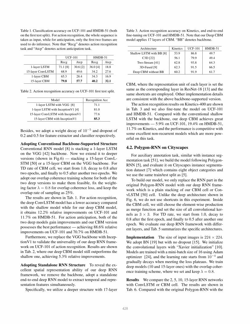
Table 1. Classification accuracy on UCF-101 and HMDB-51 (both

on the first test split). For action recognition, the whole sequence is

taken as input, while for anticipation, only the first two frames are

used to do inference. Note that “Recg” denotes action recognition

task and “Atcp” denotes action anticipation task.

UCF-101 HMDB-51

Recg Atcp Recg Atcp

1-layer LSTM 71.1 [8] 30.6 [2] 36.0 [4] 18.8

15-layer ConvLSTM 68.9 49.6 34.2 27.6

1-layer CBM 65.3 28.4 34.3 16.9

15-layer CBM 79.8 57.7 40.2 32.1

Table 2. Action recognition accuracy on UCF-101 first test split.

Model Recognition Acc

1-layer LSTM with VGG [8] 71.1

1-layer LSTM with InceptionV1 [4] 81.0

15-layer ConvLSTM with InceptionV1 77.6

15-layer CBM with InceptionV1 85.3

Besides, we adopt a weight decay of 10−5 and dropout of

0.2 and 0.5 for feature extractor and classifier respectively.

Adopting Conventional Backbone-Supported Structure

Conventional RNN model [8] is stacking a 1-layer LSTM

on the VGG [42] backbone. Now we extend it to deeper

versions (shown in Fig.6) — stacking a 15-layer ConvL-

STM [50] or a 15-layer CBM on the VGG backbone. For

TD rate of CBM cell, we start from 1.0, decay to 0.8 after

two epochs, and finally to 0.5 after another two epochs. We

adopt our overlap coherence training scheme for both of the

two deep versions to make them feasible, fix the weight-

ing factor λ = 0.8 for overlap coherence loss, and keep the

overlap rate of sampling as 25%.

The results are shown in Tab. 1. For action recognition,

the deep ConvLSTM model has a lower accuracy compared

with the shallow model while for our deep CBM model,

it obtains 12.2% relative improvements on UCF-101 and

11.7% on HMDB-51. For action anticipation, both of the

two deep models gain improvements and our CBM version

possesses the best performance — achieving 88.6% relative

improvements on UCF-101 and 70.7% on HMDB-51.

Furthermore, we replace the VGG backbone with Incep-

tionV1 to validate the universality of our deep RNN frame-

work on UCF-101 of action recognition. Results are shown

in Tab. 2, where our deep CBM model still outperforms the

shallow one, achieving 5.3% relative improvements.

Adopting Standalone RNN Structure To reveal the ex-

cellent spatial representation ability of our deep RNN

framework, we remove the backbone, adopt a standalone

end-to-end deep RNN model to extract temporal and repre-

sentation features simultaneously.

Specifically, we utilize a deeper structure with 17-layer

Table 3. Action recognition accuracy on Kinetics, and end-to-end

fine-tuning on UCF-101 and HMDB-51. Note that our Deep CBM

model applies 17 layers of CBM. “BB” denotes backbone.

Architecture Kinetics UCF-101 HMDB-51

Shallow LSTM with BB [8] 53.9 86.8 49.7

C3D [22] 56.1 79.9 49.4

Two-Stream [41] 62.8 93.8 64.3

3D-Fused [9] 62.3 91.5 66.5

Deep CBM without BB 60.2 91.9 61.7

CBM, where the representation unit of each layer is set the

same as the corresponding layer in ResNet-18 [13] and the

same shortcuts are employed. Other implementation details

are consistent with the above backbone-supported version.

The action recognition results on Kinetics-400 are shown

in Tab. 3 and we also fine-tune the model on UCF-101

and HMDB-51. Compared with the conventional shallow

LSTM with the backbone, our deep CBM achieves great

improvements — 5.9% on UCF-101, 19.4% on HMDB-51,

11.7% on Kinetics, and the performance is competitive with

some excellent non-recurrent models which are more pow-

erful on this task.

4.2. Polygon­RNN on Cityscapes

For auxiliary annotation task, similar with instance seg-

mentation task [51], we build the model following Polygon-

RNN [5], and evaluate it on Cityscapes instance segmenta-

tion dataset [7] which contains eight object categories and

we use the same train/test split as [5].

To build our model, we only replace the RNN part in the

original Polygon-RNN model with our deep RNN frame-

work which is a plain stacking of our CBM cell or Con-

vLSTM [50] cell. Unlike the deep architecture shown in

Fig. 6, we do not use shortcuts in this experiment. Inside

the CBM cell, we still choose the element-wise production

as merge function and set the size of all convolutional ker-

nels as 3 × 3. For TD rate, we start from 1.0, decay to

0.8 after the first epoch, and finally to 0.5 after another one

epoch. We evaluate our deep RNN framework with differ-

ent layers, and Tab. 5 summarizes the specific architectures.

Implementation The size of input images is 224 × 224.

We adopt BN [19] but with no dropout [15]. We initialize

the convolutional layers with “Xavier initialization” [10].

Models are trained with a mini-batch size of 16 using Adam

optimizer [24], and the learning rate starts from 10−4 and

gradually decays when meeting the loss plateaus. We train

deep models (10 and 15-layer ones) with the overlap coher-

ence training scheme, where we set and keep λ = 0.8.

Results We compare the 2, 5, 10, 15-layer RNN networks

with ConvLSTM or CBM cell. The results are shown in

Tab. 6. Compared with the original Polygon-RNN with the

428

Table 4. Video prediction results on KTH. “T1” denotes the first frame to predict and “Avg” denotes the average value.

Method Metric T1 T2 T3 T4 T5 T6 T7 T8 T9 T10 T11 T12 T13 T14 T15 T16 T17 T18 T19 T20 Avg

ConvLSTM [50]PSNR 33.8 30.6 28.8 27.6 26.9 26.3 26.0 25.7 25.3 25.0 24.8 24.5 24.2 23.7 23.2 22.7 22.1 21.8 21.7 21.6 25.3

SSIM 0.947 0.906 0.871 0.844 0.824 0.807 0.795 0.787 0.773 0.757 0.747 0.738 0.732 0.721 0.708 0.691 0.674 0.663 0.659 0.656 0.765

MCnet [45]PSNR 33.8 31.0 29.4 28.4 27.6 27.1 26.7 26.3 25.9 25.6 25.1 24.7 24.2 23.9 23.6 23.4 23.2 23.1 23.0 22.9 25.9

SSIM 0.947 0.917 0.889 0.869 0.854 0.840 0.828 0.817 0.808 0.797 0.788 0.779 0.770 0.760 0.752 0.744 0.736 0.730 0.726 0.723 0.804

OursPSNR 34.3 31.8 30.2 29.0 28.2 27.6 27.1 26.7 26.3 25.8 25.5 25.1 24.8 24.5 24.2 24.0 23.8 23.7 23.6 23.5 26.5

SSIM 0.951 0.923 0.905 0.885 0.871 0.856 0.843 0.833 0.824 0.814 0.805 0.796 0.790 0.783 0.779 0.775 0.770 0.765 0.761 0.757 0.824

Table 5. Structures of Polygon-RNN models with different depths.

# filters 256 128 64 32 8

# layers

2-layer model - - 1 - 1

5-layer model - 2 1 1 1

10-layer model - 5 3 1 1

15-layer model 2 4 6 2 1

shallow RNN, our deep CBM model achieves 14.7% rela-

tive improvements which is even competitive with Polygon-

RNN++ proposed in [1] which adopts many complex tricks,

while the deep ConvLSTM model suffers from higher train-

ing loss, leading to a bad performance.

4.3. Video Future Prediction

For video future prediction, we evaluate our deep RNN

framework using the state-of-the-art method: MCnet pro-

posed in [45], which predicts 20 future frames based on the

observed 10 previous frames. We only replace the 1-layer

ConvLSTM part of the motion encoder into our 15-layer

deep CBM model, where the TD rate is finally set to 0.5

with similar process as the above. The detailed implementa-

tion settings are consistent with the original method in [45].

We evaluate on the KTH dataset [39] which contains 600

videos for 6 human actions, and we utilize PSNR [31] and

SSIM [47] as metrics. The results are shown in Tab. 4 and

we can see that compared with the original method using

shallow RNN, our deep model achieves 1.6% improvements

on SSIM and 1.8% on PSNR for 10-frame prediction, and

2.6% on SSIM and 2.1% on PSNR for 20-frame prediction.

In this experiment, we do not adopt the overlap coher-

ence training scheme since the sequence is not too long.

5. Analysis

The above visual applications demonstrate the superior-

ity of our deep RNN framework and in this section we will

further verify the effectiveness of our detailed designs —

the model depth, CBM for deep structure, the overlap coher-

ence training scheme, merge function and TD rate of CBM.

Analysis on Depth Results of all above experiments have

already demonstrated that our deep RNN model remarkably

outperforms the shallow RNN one due to the stronger repre-

sentation capability with the depth growing. We analyze the

experiments on Polygon-RNN to further explore the spe-

Table 6. Performance (IoU in %) on Cityscapes validation set

(used as test set in [5]). Note that “Polyg-LSTM” denotes the

original Polygon-RNN structure with ConvLSTM cell and “Polyg-

CBM” denotes the Polygon-RNN structure with CBM cell.

Model IoU

Original Polygon-RNN [5] 61.4

Residual Polygon-RNN [1] 62.2

Residual Polygon-RNN + attention + RL [1] 67.2

Residual Polygon-RNN + attention + RL + EN [1] 70.2

Polygon-RNN++ [1] 71.4

# layers # params of RNN

Polyg-LSTM 2 0.47M 61.4

Polyg-LSTM 5 2.94M 63.0

Polyg-LSTM 10 7.07M 59.3

Polyg-LSTM 15 15.71M 46.7

Polyg-CBM 2 0.20M 59.9

Polyg-CBM 5 1.13M 63.1

Polyg-CBM 10 2.68M 67.1

Polyg-CBM 15 5.85M 70.4

cific relationships between the depth and the model perfor-

mance, which is illustrated in Fig. 7(a) and Fig. 7(b).

From Fig. 7(b), we can observe that utilizing CBM, the

deeper the model is built, the lower training loss and higher

IoU value we will receive. Moreover, it is worth noting that

the deep models converge as fast as the shallow ones.

Analysis on CBM As results shown in Tab. 1 and Tab. 2,

our deep CBM model achieves the best performance on ac-

tion recognition task with two different backbones and ac-

tion anticipation task, while deep ConvLSTM model suffers

from lower accuracy on action recognition even compared

with the shallow one.

As we discussed above, building deep RNN models

needs to co-adapt to both temporal and representation infor-

mation, making it difficult to optimize over a long sequence.

Therefore, for action recognition that takes the whole videos

as inputs, commonly-used deep RNN models cannot benefit

from the increased depth, while for action anticipation that

predicts only based on the first two frames, deeper structure

brings better results. To resolve this problem caused by the

contradiction of the two information flows when stacking

deep, our CBM cell is right introduced to de-couple these

two flows to make training more efficient, and receives best

results on both tasks.

429

0 50k 100k 150k 200k 250k 300k0.1

0.2

0.3

0.4

0.5

0.6

IoU

2.53.03.54.04.55.05.56.0

loss

2_layer_IoU

5_layer_IoU 10_layer_IoU15_layer_IoU

2_layer_loss 5_layer_loss 10_layer_loss 15_layer_loss

(a) Polyg-LSTM

0 50k 100k 150k 200k 250k 300k0.1

0.2

0.3

0.4

0.5

0.6

0.7

IoU

2_layer_IoU5_layer_IoU 10_layer_IoU 15_layer_IoU 2_layer_loss 5_layer_loss 10_layer_loss 15_layer_loss

2.53.03.54.04.55.05.56.0

loss

(b) Polyg-CBM (c) TD-rate comparison

Figure 7. Training on Cityscapes. Dashed lines denote training loss, and the bold lines denote testing IoU. Left: Polyg-LSTM networks.

Deep models are difficult to train and suffer from high training loss. The convergence of 15-layer is not shown. Middle: Polyg-CBM

networks adopting 0.5 TD-rate. Deep models are easy to train. Right: Comparison between different TD rates on 10 and 15-layer models.

Table 7. Classification accuracy on UCF-101 with element-wise

production and addition settings. For R, both of the two set-

tings adopt ReLU(Conv(·)). For T , production setting adopts

Sigmoid(Conv(·)) while addition adopts ReLU(Conv(·)).

Recognition Anticipation

Production 79.8 57.7

Addition 77.4 56.7

Besides, results of Polygon-RNN task in Tab. 6 also

prove that our CBM cell is more suitable for stacking deep,

and comparisons between Fig. 7(a) and Fig. 7(b) further re-

veal that using ConvLSTM to stack deep leads to higher

training loss and lower IoU value.

Analysis on Overlap Coherence Training Scheme All

the deep models above adopt our overlap coherence train-

ing scheme. From the results, we can see that it works well

— deep models are trainable on commonly-used GPUs and

all the models learn effective temporal features. Under this

scheme, though it may not transfer temporal information as

smoothly as the original training scheme, the overlaps and

the coherence loss guarantee the consistency of temporal

information among the clips to a certain degree, and finally

we do benefit from the increasing structural depth by mak-

ing some compromise on the sequence length.

Analysis on Merge Function ζ All above experi-

ments are committed with element-wise production merge

function. Here, we also evaluate another setting:

ReLU(Conv(·)) for R and T , and element-wise addition

for the merge function, which treats the two flows equally

without discrimination when merging the information. For

action recognition and anticipation tasks on UCF-101, the

comparison of these two settings is shown in Tab. 7. We find

that the production setting is marginally better than the ad-

dition one, possibly because the production setting extracts

better spatial representation features that are more useful for

video classification problems.

Analysis on TD Rate To show the influence of TD rate,

we set the final TD rate to 0.0, 0.2, 0.5, 0.8 and 1.0 (grad-

ually decay as the above experiments) and results of action

recognition task on UCF-101 are shown in Tab. 8. We can

Table 8. Action recognition accuracy on UCF-101 with different

TD rates. We use VGG19 as backbones, 15-layer CBM as the

RNN part, and element-wise production as merge function.

TD rate Acc TD rate Acc TD rate Acc

0.0 75.2 0.5 79.8 1.0 75.3

0.2 76.5 0.8 77.1

see that 0.5 TD-rate achieves the best result. When the TD

rate is set to 1.0, the temporal information can only flow

backward in its own layer, forbidding the temporal commu-

nication among different layers, thus leading to a relatively

non-ideal performance. For Polygon-RNN task, the results

shown in Fig. 7(c) reveal consistent conclusions.

6. Conclusion

In this paper, we proposed a deep RNN framework for

visual sequential applications. The first part of our deep

RNN framework is the CBM structure designed to balance

the temporal flow and representation flow. Based on the

characteristics of these two flows, we proposed the Tem-

poral Dropout to simplify the training process and enhance

the generalization ability. The second part is the Overlap

Coherence Training Scheme aiming at resolving the large

resource consuming of deep RNN models, which can sig-

nificantly reduce the length of sequences loaded into the

model and guarantee the consistency of temporal informa-

tion through overlaps simultaneously.

We conducted extensive experiments to evaluate our

deep RNN framework. Compared with the conventional

shallow RNN, our deep RNN framework achieves remark-

able improvements on action recognition, action anticipa-

tion, auxiliary annotation and video future prediction tasks.

Comprehensive analysis is presented to further validate the

effectiveness and robustness of our specific designs.

7. Acknowledgements

This work is supported in part by the National Key R&D

Program of China, No. 2017YFA0700800, National Natu-

ral Science Foundation of China under Grants 61772332.

430

References

[1] D. Acuna, H. Ling, A. Kar, and S. Fidler. Efficient interactive

annotation of segmentation datasets with polygon-rnn++. In

CVPR, pages 859–868, 2018.

[2] M. S. Aliakbarian, F. S. Saleh, M. Salzmann, B. Fernando,

L. Petersson, and L. Andersson. Encouraging lstms to antic-

ipate actions very early. In ICCV, volume 1, 2017.

[3] Y. Bian, C. Gan, X. Liu, F. Li, X. Long, Y. Li, H. Qi, J. Zhou,

S. Wen, and Y. Lin. Revisiting the effectiveness of off-the-

shelf temporal modeling approaches for large-scale video

classification. arXiv preprint, 2017.

[4] J. Carreira and A. Zisserman. Quo vadis, action recognition?

a new model and the kinetics dataset. In CVPR, pages 4724–

4733. IEEE, 2017.

[5] L. Castrejon, K. Kundu, R. Urtasun, and S. Fidler. Annotat-

ing object instances with a polygon-rnn. In CVPR, volume 1,

page 2, 2017.

[6] K. Cho, B. Van Merrienboer, C. Gulcehre, D. Bahdanau,

F. Bougares, H. Schwenk, and Y. Bengio. Learning phrase

representations using rnn encoder-decoder for statistical ma-

chine translation. arXiv preprint, 2014.

[7] M. Cordts, M. Omran, S. Ramos, T. Rehfeld, M. Enzweiler,

R. Benenson, U. Franke, S. Roth, and B. Schiele. The

cityscapes dataset for semantic urban scene understanding.

In CVPR, pages 3213–3223, 2016.

[8] J. Donahue, L. Anne Hendricks, S. Guadarrama,

M. Rohrbach, S. Venugopalan, K. Saenko, and T. Dar-

rell. Long-term recurrent convolutional networks for visual

recognition and description. In CVPR, pages 2625–2634,

2015.

[9] C. Feichtenhofer, A. Pinz, and A. Zisserman. Convolutional

two-stream network fusion for video action recognition. In

CVPR, pages 1933–1941, 2016.

[10] X. Glorot and Y. Bengio. Understanding the difficulty of

training deep feedforward neural networks. In Conference on

Artificial Intelligence and Statistics, pages 249–256, 2010.

[11] C. Gu, C. Sun, S. Vijayanarasimhan, C. Pantofaru, D. A.

Ross, G. Toderici, Y. Li, S. Ricco, R. Sukthankar, C. Schmid,

et al. Ava: A video dataset of spatio-temporally localized

atomic visual actions. arXiv preprint, 3(4):6, 2017.

[12] K. He, G. Gkioxari, P. Dollar, and R. Girshick. Mask r-cnn.

In ICCV, pages 2980–2988. IEEE, 2017.

[13] K. He, X. Zhang, S. Ren, and J. Sun. Deep residual learning

for image recognition. In CVPR, pages 770–778, 2016.

[14] M. Hermans and B. Schrauwen. Training and analysing deep

recurrent neural networks. In NIPS, pages 190–198, 2013.

[15] G. E. Hinton, N. Srivastava, A. Krizhevsky, I. Sutskever, and

R. R. Salakhutdinov. Improving neural networks by prevent-

ing co-adaptation of feature detectors. arXiv preprint, 2012.

[16] S. Hochreiter and J. Schmidhuber. Long short-term memory.

Neural Computation, 9(8):1735–1780, 1997.

[17] R. Hou, C. Chen, and M. Shah. Tube convolutional neu-

ral network (t-cnn) for action detection in videos. In ICCV,

2017.

[18] P.-S. Huang, M. Kim, M. Hasegawa-Johnson, and

P. Smaragdis. Joint optimization of masks and deep recurrent

neural networks for monaural source separation. IEEE/ACM

Transactions on Audio, Speech, and Language Processing,

23(12):2136–2147, 2015.

[19] S. Ioffe and C. Szegedy. Batch normalization: Accelerating

deep network training by reducing internal covariate shift.

arXiv preprint, 2015.

[20] O. Irsoy and C. Cardie. Deep recursive neural networks for

compositionality in language. In NIPS, pages 2096–2104,

2014.

[21] O. Irsoy and C. Cardie. Opinion mining with deep recurrent

neural networks. In EMNLP, pages 720–728, 2014.

[22] S. Ji, W. Xu, M. Yang, and K. Yu. 3d convolutional neural

networks for human action recognition. TPAMI, 35(1):221–

231, 2013.

[23] A. Karpathy, G. Toderici, S. Shetty, T. Leung, R. Sukthankar,

and L. Fei-Fei. Large-scale video classification with convo-

lutional neural networks. In CVPR, pages 1725–1732, 2014.

[24] D. P. Kingma and J. Ba. Adam: A method for stochastic

optimization. arXiv preprint, 2014.

[25] A. Krizhevsky, I. Sutskever, and G. E. Hinton. Imagenet

classification with deep convolutional neural networks. In

NIPS, pages 1097–1105, 2012.

[26] H. Kuehne, H. Jhuang, E. Garrote, T. Poggio, and T. Serre.

Hmdb: a large video database for human motion recognition.

In ICCV, pages 2556–2563. IEEE, 2011.

[27] J. Li, C. Wang, H. Zhu, Y. Mao, H.-S. Fang, and C. Lu.

Crowdpose: Efficient crowded scenes pose estimation and

a new benchmark. arXiv preprint, 2018.

[28] Y.-L. Li, S. Zhou, X. Huang, L. Xu, Z. Ma, H.-S. Fang, Y.-

F. Wang, and C. Lu. Transferable interactiveness prior for

human-object interaction detection. arXiv preprint, 2018.

[29] Z. Li, K. Gavrilyuk, E. Gavves, M. Jain, and C. G. Snoek.

Videolstm convolves, attends and flows for action recogni-

tion. Computer Vision and Image Understanding, 166:41–

50, 2018.

[30] X. Long, C. Gan, G. de Melo, J. Wu, X. Liu, and S. Wen.

Attention clusters: Purely attention based local feature inte-

gration for video classification. In CVPR, pages 7834–7843,

2018.

[31] M. Mathieu, C. Couprie, and Y. LeCun. Deep multi-scale

video prediction beyond mean square error. arXiv preprint,

2015.

[32] J. Oh, X. Guo, H. Lee, R. L. Lewis, and S. Singh. Action-

conditional video prediction using deep networks in atari

games. In NIPS, pages 2863–2871, 2015.

[33] B. Pan, W. Lin, X. Fang, C. Huang, B. Zhou, and C. Lu.

Recurrent residual module for fast inference in videos. In

CVPR, 2018.

[34] B. Pang, K. Zha, and C. Lu. Human action adverb recog-

nition: Adha dataset and a three-stream hybrid model. In

CVPR Workshops, pages 2325–2334, 2018.

[35] R. Pascanu, C. Gulcehre, K. Cho, and Y. Bengio. How to

construct deep recurrent neural networks. arXiv preprint,

2013.

[36] J. Redmon and A. Farhadi. Yolov3: An incremental improve-

ment. arXiv preprint, 2018.

431

[37] O. Russakovsky, J. Deng, H. Su, J. Krause, S. Satheesh,

S. Ma, Z. Huang, A. Karpathy, A. Khosla, M. Bernstein,

et al. Imagenet large scale visual recognition challenge.

IJCV, 115(3):211–252, 2015.

[38] H. Sak, A. Senior, and F. Beaufays. Long short-term memory

recurrent neural network architectures for large scale acous-

tic modeling. In Conference of the International Speech

Communication Association, 2014.

[39] C. Schuldt, I. Laptev, and B. Caputo. Recognizing human

actions: a local svm approach. In CVPR, volume 3, pages

32–36. IEEE, 2004.

[40] P. Sermanet, D. Eigen, X. Zhang, M. Mathieu, R. Fergus,

and Y. LeCun. Overfeat: Integrated recognition, localization

and detection using convolutional networks. arXiv preprint,

2013.

[41] K. Simonyan and A. Zisserman. Two-stream convolutional

networks for action recognition in videos. In NIPS, pages

568–576, 2014.

[42] K. Simonyan and A. Zisserman. Very deep convolutional

networks for large-scale image recognition. arXiv preprint,

2014.

[43] K. Soomro, A. R. Zamir, and M. Shah. Ucf101: A dataset

of 101 human actions classes from videos in the wild. arXiv

preprint, 2012.

[44] S. Venugopalan, H. Xu, J. Donahue, M. Rohrbach,

R. Mooney, and K. Saenko. Translating videos to natural lan-

guage using deep recurrent neural networks. arXiv preprint,

2014.

[45] R. Villegas, J. Yang, S. Hong, X. Lin, and H. Lee. Decom-

posing motion and content for natural video sequence pre-

diction. arXiv preprint, 2017.

[46] L. Wang, Y. Qiao, X. Tang, and L. Van Gool. Actionness esti-

mation using hybrid fully convolutional networks. In CVPR,

pages 2708–2717, 2016.

[47] Z. Wang, A. C. Bovik, H. R. Sheikh, and E. P. Simoncelli.

Image quality assessment: from error visibility to struc-

tural similarity. IEEE Transactions on Image Processing,

13(4):600–612, 2004.

[48] P. Weinzaepfel, Z. Harchaoui, and C. Schmid. Learning to

track for spatio-temporal action localization. In ICCV, pages

3164–3172, 2015.

[49] Z. Wu, X. Wang, Y.-G. Jiang, H. Ye, and X. Xue. Modeling

spatial-temporal clues in a hybrid deep learning framework

for video classification. In ACM International Conference on

Multimedia, pages 461–470. ACM, 2015.

[50] S. Xingjian, Z. Chen, H. Wang, D.-Y. Yeung, W.-K. Wong,

and W.-c. Woo. Convolutional lstm network: A machine

learning approach for precipitation nowcasting. In NIPS,

pages 802–810, 2015.

[51] W. Xu, Y. Li, and C. Lu. Srda: Generating instance segmen-

tation annotation via scanning, reasoning and domain adap-

tation. In ECCV, pages 120–136, 2018.

[52] J. Yue-Hei Ng, M. Hausknecht, S. Vijayanarasimhan,

O. Vinyals, R. Monga, and G. Toderici. Beyond short snip-

pets: Deep networks for video classification. In CVPR, pages

4694–4702, 2015.

[53] M. D. Zeiler and R. Fergus. Visualizing and understanding

convolutional networks. In ECCV, pages 818–833. Springer,

2014.

432