Watersheds: Management, Restoration and Environmental Impact $145.00

Editors: Jeremy C. Vaughn

Book Description: A watershed is the area of land from which precipitation or surface water flow is drained into a receiving water body. The term is roughly analogous to a "drainage basin", and are often used interchangeably. While primarily describing the geologic/geographic drainage patterns of water, a more holistic view of the word watershed incorporates all the biotic and abiotic communities and processes contained in the drainage basin. Watersheds may be referred to as the sum of the area, drainage patterns, and environment of a given waterway or waterway segment. This book reviews research on watersheds including the climatic change impacts on the hydrologic dynamics of watershed systems; the watershed approach for resource conservation, environment quality and food security in the Indian Himalayas and others.

Table of Contents: Preface Watershed Approach for Resource Conservation, Environment Quality and Food Security in the Indian Himalayas (U. C. Sharma, M. Datta, Vikas Sharma, Centre for Natural Resources Management, V. P. O. Tarore, District Jammu, India, and others) Modeling Soil Erosion Processes in Watersheds and the Relation between Soil Loss with Geomorphic and Chemical Parameters (Maria Kouli, Despina Kalisperi, Pantelis Soupios, Filippos Vallianatos, Technological Educational Institute of Crete, Department of Natural Resources and Environment, Laboratory of Geoinformatics and Laboratory of Applied Geophysics and Seismology, Chalepa, Chania, Crete, Greece) Watershed Management: A Geospatial Technology Perspective (R.S Dwivedi, T. Ravisankar, National Remote Sensing Centre, Indian Space Research Organization, Balanagar Hyderabad, Andhra Pradesh, India)

Click to enlarge

Robust Methods of Segmentation for Biomedical Images (Roberto Rodríguez Morales, Institute of Cybernetics, Mathematics & Physics (ICIMAF), Digital Signal Processing Group, Ciudad Habana, Cuba) Evaluation of Watershed Stress in an Urbanized Landscape in Southern Lake, Michigan (Charles C. Morris, Thomas P. Simon, Department of Biology, Indiana State University, Terre Haute, Indiana) Modeling for Watershed Planning, Management, and Decision Making (Ali Mirchi, David W. Watkins, Jr., Kaveh Madani, Department of Civil & Environmental Engineering, Michigan Technological University, Houghton, Michigan, and others) Historic Water Resources Development in the Río Fajardo Basin, Puerto Rico, and Potential Hydrologic Implications of Recent Changes in River Management (Jorge R. Ortiz-Zayas, José Juan Terrasa-Soler, Lymarie Urbina, Institute for Tropical Ecosystem Studies, University of Puerto Rico, San Juan, P.R., and others) A Hydrogeochemical and Isotope Investigation of the River Sava Watershed (Nives Ogrinc, Tjaša Kanduè, Dušan Goloboèanin, David Kocman, Nada Miljeviæ, Department of Environmental Sciences, Jožef Stefan Institute, Ljubljana, Slovenia, and others) Climatic Change Impacts on Hydrologic Dynamics of Watershed Systems (Timothy O. Randhir, Paul Ekness, Olga Tsvetkova, Department of Natural Resources, University of Massachusetts, Amherst, Massachusetts) Mainstreaming a Decade’s Experiences in Watershed Management to Meet the Challenges of Environmental Change in the Hindu Kush-Himalayas (Isabelle Providoli, Keshar Man Sthapit, Madhav Dhakal, Eklabya Sharma, International Centre for Integrated Mountain Development (ICIMOD), Kathmandu, Nepal) A Modified Ecological Footprint Model and its Application to Agro-Economic Ecosystem Before and After Grain for Green Policy in the Watershed Scale on the Loess Plateau in China (Zhou Ping, Zhuang Wenhua, Liu Guo-Bin,Wen Anbang, He Xiubin,Wang Bing, Institute of Mountain Hazards and Environment, Chinese Academy of Sciences, Chengdu, China, and others) A New Clustering Algorithm for Color Image Segmentation (Mohammed Talibi Alaoui, Abderrahmane Sbihi, Laboratoire de Recherche en Informatique LARI, Université Mohamed I, Oujda, Morocco, and others) Evaluation on Land Potential and Bearing Capacity after Returning Farmland to Forest in Gezhen’er Watershed (Zhang You-Yan, Cheng Jin-hua, Zhou Ze-fu, Research Institute of Forestry, Chinese Academy of Forestry, Beijing, China, and others) Optimization approaches to nonpoint pollutant source control in watersheds ^ (Shigeya Maeda, Toshihiko Kawachi, Koichi Unami, Junichiro Takeuchi Graduate School of Agriculture, Kyoto University, Japan)

Correlations of Surface and Groundwater Flow with Nitrate-N Concentration in Agricultural Drainage Ditches in Two Illinois Watersheds (Debashish Goswami, Prasanta K. Kalita, Department of Agricultural and Biological Engineering, South-West Florida Research and Education Center, University of Florida, Immokalee, Florida, and others) Short Communication: Low Impact Development for Sustainable Watershed Management (Chia-Ling Chang, Department of Water Resources Engineering and Conservation, Feng Chia University; Taichung, Taiwan, R.O.C) Index

Series: Environmental Science, Engineering and Technology Binding: ebook Pub. Date: 2010 - 3rd Quarter Pages: 7 x 10 ISBN: 978-1-61209-295-9 Status: AV

Modeling Soil Erosion Processes in Watersheds and the Relation between Soil Loss with Geomorphic and Chemical Parameters Maria Kouli1, Despina Kalisperi1, Pantelis Soupios1, Filippos Vallianatos1 1Technological Educational Institute of Crete, Department of Natural Resources and Environment, Laboratory of Geoinformatics and Laboratory of Applied Geophysics and Seismology

Corresponding author: Dr. Maria Kouli, tel.: 00302821023028, fax: 00302821023042, email: mkouli@chania.teicrete.gr, addrs: Technological Educational Institute of Crete, 3 Romanou 73133, Chalepa, Chania, Crete, GREECE Abstract

Soil erosion by water has led to severe economic and environmental impacts and remains a global issue because of its extent and complex processes. Loss of soil nutrients, declining crop yields, and reduction in soil fertility are only a few problems that caused by soil erosion. In watershed areas soil, moved by erosion, carries dangerous chemicals into rivers, streams, and groundwater resources, while simultaneously it causes a reduction in water-bearing capacity of an aquifer as well as in the groundwater quality. An effort to understand soil erosion processes is carried out in the present study.

In a first step, the Revised Universal Soil Loss equation (RUSLE) model is adopted in a Geographical Information System (GIS) framework in order to predict the potential annual soil loss for several major watersheds of Crete Island, southern Greece, where soil erosion is a growing problem. The RUSLE factors were calculated (in the form of raster layers and in a cell by cell basis) for seven major watersheds which cover the northeastern and central part of the Chania and Rethymnon Prefectures, respectively. The R-factor was calculated from monthly and annual precipitation data. The K-factor was estimated using the soil data available from the Soil Geographical Data Base of Europe at a scale of 1:1,000,000. The LS-factor was extracted from a 20-meters digital elevation model (DEM) of the study area. The C-factor was calculated through the Normalized Difference Vegetation Index (NDVI) approach using Remote Sensing (RS) techniques while the Practice Support factor was set to 1. The results show that an extended part of the area is undergoing severe erosion. The mean annual soil loss is predicted more than ~200 (t/ha yr) for Kalami and Argyroupolis watersheds while Vrysses watershed exhibits annual soil loss more than 300 t/ha yr, showing extended erosion and demanding the attention of local administrators.

In a next step, possible relation of soil loss raster layers (with a cell size of 20*20 meters) spatial distribution with structural, geomorphic and chemical parameters of the watersheds is investigated. Specifically, data derived from Remote Sensing (such as NDVI), interpolated point data (e.g., borehole data, chemical data) slope angle, geological and permeability data are fully integrated in a GIS environment. Ordinary Least Squares linear regression is finally applied for analyzing the relationships between the soil loss and the unique parameters. Finally, the obtained results provide information for an improved understanding of soil erosion processes in watersheds.

Introduction Soil erosion is a natural occurring process and is one form of soil degradation.

Other kinds of soil degradation include salinisation, nutrient loss, and compaction (Favis-Mortlock 2007). Soil can be eroded mainly by wind and water, each contributing a significant amount of soil loss each year worldwide. High winds can blow away loose soils from flat or hilly terrain, while erosion, due to the energy of water, occurs when water it falls toward the earth and flows over the surface. In general, geological erosion removes soil at roughly the same rate as soil is formed. On the other hand, 'accelerated' soil erosion - loss of soil at a much faster rate than it is formed - is a recent problem which is related with mankind's unwise actions (wrong agricultural and cultivation practices, excessive deforestation, overgrazing, etc), leaving the land unprotected (Keller 1996; Renschler and Harbor 2002).

Problems caused by soil erosion include loss of soil nutrients, declining crop yields, reduction in soil productivity (Renard et al. 1997). Moreover, soil moved by erosion carries nutrients, pesticides and other harmful farm chemicals into rivers, streams, and ground water resources (Nyakatawa et al. 2001) and as a result, protecting soils from erosion is important to sustain human life. Finally, soil erosion causes air pollution through emissions of radioactive gases such as carbon dioxide (CO2), methane (CH4), and nitrous oxide (N2O) (Lal 2001; Boyle 2002).

As it is already mentioned, soil erosion is a serious problem worldwide, with inestimable economic and environmental impacts because of its extent, magnitude, rate, and complex processes (Lal 1994). Numerous human-induced activities, such as mining, construction, and agricultural activities, disturb land surfaces, resulting in erosion. Soil erosion from cultivated areas is typically higher than that from uncultivated areas (Brown, 1984). Soil erosion can pose a great concern to the environment because cultivated areas can act as a pathway for transporting nutrients, especially phosphorus attached to sediment particles to river systems (Ouyang and Bartholic 1997).

There are four basic types of erosion by water: 1) Sheet Erosion, the removal of a fairly uniform layer of soil from the land surface by the action of rainfall and surface runoff, 2) Rill Erosion, the formation of numerous small waste channels, occurring primarily on recently cultivated soil, 3) Gully Erosion, an advanced state of rill erosion in which water accumulates in channels and washes away soil to depths ranging from one to two feet to as much as 75 to 100 feet, and 4) Streambed Erosion, the widening of streams (Blanpied 1984).

Estimation of soil erosion is of vital importance in managing and conserving natural resources. Various approaches and equations for risk assessment on soil erosion by water are available in international literature.

The collection of empirical data on erosion over a wide area is costly, laborious and time consuming due to the fact that the erosion process varies widely across soils, climate, topography, and management (Zake 1993; Tenywa and Lal 1994; Bekunda and Woomer 1996; Osinde 1996; Tenywa et al. 1999). Because of the difficulty in measuring point-to-point erosion resulting from the wide spatial and temporal variability in its factor controls, efforts targeting improved erosion management through identification and development of useful customized remedial measures are greatly facilitated by predictive models (Lufafa et al. 2003).

A wide variety of models are available for assessing soil erosion risk. Erosion models can be classified in a number of ways. One may make a subdivision based on the time scale for which a model can be used: some models are designed to predict long-term annual soil losses, while others predict single storm losses (event-based). Another distinction can be made between lumped models that predict erosion at a single point, and spatially distributed models. Alternatively, a useful division is the one between empirical and physically-based models. To sum up, the choice for a particular model largely depends on the purpose for which it is intended and the available data, time and money (Grimm et al. 2002). Table I gives a short description of the most commonly used computer-based erosion models.

Mapping soil erosion in large areas is often very difficult using traditional methods. The use of remote sensing (RS) and geographical information system (GIS) techniques makes soil erosion estimation and its spatial distribution feasible with reasonable costs and better accuracy in larger areas (Millward and Mersey 1999; Wang et al. 2003). GIS is defined as a computer-assisted mapping and cartographic application, a set of spatial-analytical tools, a type of database systems, or a field of academic study (Lo and Yeung 2003). Geographical data are used to solve various spatial problems, while the skills and procedures for collecting, managing, and using geographic information entails a comprehensive body of scientific knowledge from which these skills and procedures are developed (Lo and Yeung 2003). Additionally, remote sensing can be defined as the observation of targets or processes from a distance, without being in a physical contact with the target. Thus, remote sensing also includes data analysis which involves the methods and processes for extracting meaningful spatial information from the remotely sensed data for direct input to a geographic information system. In RS, conventional aerial photography and satellite remote sensing instruments that obtain pictures of visible, near-infrared (NIR) and thermal infrared (TIR) energy belong to passive remote sensing techniques, while the radar and lidar belong to active remote sensing techniques (Kouli et al. 2008)|. For example, a combination of remote sensing, GIS, and RUSLE provides the potential to estimate soil erosion loss on a cell-by-cell basis (Millward and Mersey 1999, Kouli et al. 2009). Moreover, the combined use of GIS and erosion models, such as USLE/RUSLE, has been proved an effective approach for estimating the magnitude and spatial distribution of erosion (Mitasova et al. 1996; Molnar and Julien 1998; Cox and Madramootoo 1998; Millward and Mersey 1999; Yitayew et al. 1999; Gong 2001; Wu and Dong 2001; Fernandez et al. 2003; Lewis et al. 2005; Lim et al. 2005; Fu et al. 2006; Wu and Wang 2007; Erdogan et al. 2007, Kouli et al. 2009). Such methods provide significantly better results than using traditional methods (Lu et al. 2004).

Plenty of recent projects exist globally, where researchers used different kind of tools for predicting soil erosion, attesting the immense need of this issue. For example, Lu el al. (2001) at their report predict an Australian-wide sheet and rill erosion, showing that the northern part of the country has higher erosion potential than the south, and soil erosion and the consequent reduction of productivity is a major issue in Australia too. In addition, Mutua et al. (2006) applied the RUSLE and the Hillslope Sediment Delivery Distributed (HSDD) models embedded in a GIS for predicting soil erosion and sediment yield of Masinga catchment in Kenya. The results showed the two models can serve as a useful tool in natural resources management and planning. Another project that soil

erosion estimation was attempted, was established at the Alabama Experiment Station (USA) by Nyakatawa et al. (2007) using the RUSLE 2.0 computer model.

Soil erosion by water is an extensive problem, which also curse Europe with. The Council of Europe provides an overview of the extent of soil degradation in Europe (as a technical report) using revised Global Assessment of Human Induced Soil Degradation (GLASOD) digital data (Oldeman et al. 1991; Van Lynden 1995). The most dominant effect is the loss of topsoil, which in many cases is potentially very damaging. The most important physical factors in the process of soil erosion are climate, topography and soil characteristics.

Especially southern Europe, and particularly the Mediterranean region, is extremely incline to erosion as it suffers from long dry periods followed by heavy erosive rainfall, falling on steep slopes with fragile soils, resulting in considerable amounts of erosion (Onori et al. 2006). In some parts of the Mediterranean region, erosion has reached a stage of irreversibility while in some places there is no more soil left. With a slow rate of soil formation, any soil loss of more than 1 t/ha/yr can be considered as irreversible within a time span of 50-100 years. Losses of 20 to 40 t/ha in individual storms (that may happen once every two or three years), are measured regularly in Europe with losses of more than 100 t/ha measured in extreme events (Morgan 1992). In the eastern part of the Mediterranean (Israel and the Palestinian Autonomous Areas), gradual land degradation is currently taking place, as a result of rapid socio-economic changes, an increase of population, and wrong adopted conservation measures and the misuse of land (Abu Hammad 2005).

In Greece, soil erosion affects 3.5 million hectares experience a situation amounting to 26.5% of the country’s total land area (Mitsios et al. 1995). Arhonditsis et al. (2002) studied the applicability of 3 mathematical models, including RUSLE, for predicting nonpoint source nutrient loading from agricultural watersheds of the Mediterranean region (gulf of Gera Basin) using experimental field plot data, resulting the relatively good agreement between simulated and experimental data.

Concerning Crete, an effort to predict potential annual soil loss has been conducted by Kouli et al. (2009) in nine major watersheds in the southern part of the island using RUSLE model, showing that an extent part of the study area is undergoing severe erosion. Table I. Short description of the most frequently used soil erosion models (modified from http://soilerosion.net/) AGNPS - Agricultural Non-Point Source pollution model

Agricultural Non-Point Source Pollution Model (AGNPS) is a joint USDA - Agricultural Research Service (ARS) and Natural Resources Conservation Service system of computer models developed to predict non point source pollutant loadings within agricultural watersheds. It contains a continuous simulation surface runoff model designed to assist with determining BMPs, the setting of TMDLs, and for risk & cost/benefit analyses. More detailed descriptions of the components, with example datasets, and the programs can be found at the AGNPS download page.

ANSWERS - Areal The ANSWERS (Areal Nonpoint Source Watershed

Nonpoint Source Watershed Environment Response Simulation

Environment Response Simulation) model is designed to simulate the behavior of watersheds which are mainly agricultural during and immediately after a rainfall event. Its primary application is in planning and evaluating various strategies for controlling pollution from intensively cultivated areas. Several variables are defined for each element, e.g. slope angle, aspect, soil parameters (porosity, moisture content, field capacity, infiltration capacity, erodibility factor), crop variables (coverage, interception capacity, USLE C/P factor), surface variables (roughness and surface retention) and channel variables (width and roughness). A rainfall event is simulated with time increments of one minute, taking into account spatial and temporal variability of rainfall. Several physically based mathematical relationships are used to describe interception, infiltration, surface retention, drainage, overland flow, channel flow, subsurface flow, detachment by rainfall, and/or overland flow and sediment transport by overload flow (interrill erosion).

CREAMS - Chemicals, Runoff and Erosion from Agricultural Management Systems

CREAMS is a field scale model for predicting runoff, erosion, and chemical transport from agricultural management systems. It is applicable to field-sized areas. CREAMS can operate on individual storms but can also predict long term averages (2-50 years). The objectives of the model are: 1) the model must be physically based, 2) the model must be simple, easily understood with as few parameters as possible and still represent the physical system relatively accurately, 3) the model must estimate runoff, percolation, erosion, and dissolved and adsorbed plant nutrients and pesticides and, 4) the model must distinguish between management practices. If hourly or breakpoint rainfall data are available, an infiltration-based model is used to simulate runoff. Water movement through the soil profile is modeled using a simple capacity approach, with flow occurring when a layer exceeds field capacity. The erosion component maintains elements of the USLE, but includes sediment transport capacity for overland flow. The plant nutrient sub-model of CREAMS has a nitrogen component that considers mineralization, nitrification, and denitrification processes. Several of the equations developed for the CREAMS model have been used or modified within other models, such as WEPP, SWRRB, SWAT, SWIM.

EPIC - Erosion-Productivity Impact Calculator

The EPIC (Erosion-Productivity Impact Calculator) model was developed by the Agricultural Research Service (United States Department of Agriculture) at the beginning of 1980’s. The model comprises physically based components for simulating erosion, plant growth, and related processes and economic components for assessing the cost of erosion, determining optimal management strategies. EPIC simulates the physical

processes simultaneously and realistically using readily available inputs. The physical components of EPIC can be placed into seven major divisions: hydrology, meteorology, erosion, nutrients, plant growth, soil temperature, and tillage. It has produced reasonable results under a variety of climatic conditions, soil characteristics, and management practices. It also has demonstrated sensitivity to erosion in terms of reduced crop production. Although designed to be used in the Resources Conservation Act analysis of the current status of soil and water resources in the United States, EPIC has additional potential uses, including: (1) national-level conservation policy studies; (2) national-level program planning and evaluation; (3) project-level planning and design; and (4) as a research tool.

GLEAMS The GLEAMS model consists of four components operating simultaneously: hydrology, erosion/sediment yield, pesticides and plant nutrients. The principal use of the model is to evaluate the differences among management systems rather than to predict the absolute quantities of water, soil erosion, and chemicals lost from the field. Examples of GLEAMS applications to assess management alternatives are numerous and extended bibliography can be foun in Knisel and Turtola (2000). Hydrology. Daily water accounting is simulated in a soil system layered within the genetic horizons of the root zone. The model distributes soil characteristics into a maximum of 12 computational layers with input from a maximum of 5 soil horizons. Runoff is calculated using a modified Soil Conservation Service curve number procedure. The modification mainly consists of replacing the 5-day antecedent rainfall with available soil water storage, and making the procedure a daily simulation rather than a design-type storm. Percolation through the soil layers uses a storage-routing technique. Erosion. The erosion component of GLEAMS is the Onstad–Foster modification (Onstand and Foster 1975) of the universal soil loss equation (USLE) for storm-by-storm simulation. Rill and inter-rill erosion are calculated on the non-uniform slope of a representative overland flow element of the field. The erosivity factor (R) of the USLE is replaced by storm-by-storm rainfall energy calculated from daily rainfall. The management factors of the USLE, i. e. soil loss ratio (C factor) and practice factor (P), are maintained. In addition to the overland flow element, concentrated or channel flow can be represented in the field. Plant nutrients. The plant nutrient component of GLEAMS considers comprehensive N and P cycles. Much of the nutrient component is very similar to the EPIC model except the animal

waste component. Pesticides. A pesticide component is included in the GLEAMS model (Leonard and Knisel 1989), but further information is not included here since pesticides are not a part of the present study.

KINEROS - Kinematic Runoff and Erosion Model

The kinematic runoff and erosion model KINEROS is an event based, physical model describing the processes of interception, infiltration, surface runoff and erosion from small agricultural and urban watersheds. The watershed is represented by a cascade of planes and channels; the partial differential equations describing overland flow, channel flow, erosion and sediment transport are solved by finite difference techniques. The spatial variation of rainfall, infiltration, runoff, and erosion parameters can be accommodated. KINEROS may be used to determine the effects of various artificial features such as urban developments, small detention reservoirs, or lined channels on flood hydrographs and sediment yield. Basic Elements of KINEROS. It uses one-dimensional kinematic equations to simulate flow over rectangular planes and through trapezoidal open channels, circular conduits and small detention ponds. Generally, the KINEROS is a distributed model. Multi-gage rainfall input is distributed by assigning rain gages to overland flow planes. The infiltration algorithm is dynamic, interacting with both rainfall and surface water in transit. Channel transmission losses are also included. Rain splash and hydraulic erosion are an option for overland flow planes; hydraulic erosion for channels. Eroded sediment may be routed through any type of element, even those with non eroding surfaces. KINEROS2 can automatically interpolate multi-gage rainfall intensity input to each routing element based on the spatial relationship between the element's areal centroid and the rain gage network. Data from the nearest three gages which enclose the centroid determine a plane in (x, y, z) space, where z is accumulated depth, for each time, from which the intensity at the centroid is computed. If the centroid lies outside of the network, and certain geometric criteria are met, two gages are used. Otherwise, data from the closest gage alone is used.

LISEM - LImburg Soil Erosion Model

The LImburg Soil Erosion Model (LISEM) is a physically-based runoff and erosion model for research, planning and conservation practices. It simulates the spatial effects of rainfall events mainly on small watersheds.

RillGrow Soil Erosion Models

Emergence and erosion. The eroding hillslope may be conceptualized as a self-organizing system. Antecedent micro-topography determines preferential paths for overland flow and hence the spatial pattern of surface lowering; this in turn influences the path of subsequent flow. This cycle of events

constitutes a positive feedback loop operating at a 'local' scale which, if repeated a sufficient number of times, generates a 'global' response from the system: the formation of a rill network. Viewed from this perspective, the rill network is an 'emergent' whole-system result which arises from a great many local interactions. Modeling rill erosion as a self-organizing system. Erosion models embodying such a self-organizing systems approach do not suffer from an unrealistic requirement of earlier models: the need to pre-specify rill characteristics for an initially unrilled surface. Additionally, it appears that the local interactions between the soil's surface, flow, and transported sediment need only be described in a relatively simple manner. This leads to models with modest data requirements yet strong generality and predictive power. A disadvantage, however, is the considerable computational requirement of such models. RillGrow 1 was the first, very simple, attempt at constructing a model for rill initiation and development using these concepts. It uses data on initial micro-topography to generate realistic rill patterns; however, it does not operate within a true time domain. The RillGrow 2 model similarly uses data for initial micro-topography of an unrilled area to predict rill patterns, as well as flow/sediment transport characteristics. While it represents the processes of flow and erosion more realistically than does RillGrow 1, it is still a relatively simple model. Also, several validation studies have been carried out. In these, simulated rill patterns and data for flow rate/depth etc. are compared with real-world rill data from small plots and flumes. The results are very encouraging, and are currently being written up.

RUSLE2 RUSLE2 is an advanced, computer based model that predicts long-term, average-annual erosion by water. It runs under Windows, and can be used for a broad range of farming, conservation, mining, construction, and forestry sites. Its origin was the widely-used DOS-based Revised Universal Soil Loss Equation (RUSLE). The extensive climate, soil, vegetation, and cropping management databases available for that model are currently being enhanced, prior to deploying RUSLE2 in several thousand USDA NRCS field offices. RUSLE2's engine is adaptive -- the model continually shrinks or expands as outputs are hidden or requested. It immediately provides output from default inputs and refines the output if the user can provide more specific data. Information is grouped into reusable "objects" (vegetations, soils, climates, field operations, etc.) that an average user understands.RUSLE2 can be run as a standalone application, from a third-party application, from a browser, or from an MS

Word document with pictures and text. Because of its view customization, modeling engine, widespread adoption, and extensive data support, the RUSLE2 platform is ideal for delivering a variety of environmental models.

SWAT SWAT is a river basin scale model developed to quantify the impact of land management practices in large, complex watersheds. SWAT is a public domain model actively supported by the USDA Agricultural Research Service at the Grassland, Soil and Water Research Laboratory in Temple, Texas, USA.

WATEM WATEM is a spatially distributed model capable to simulate erosion and deposition by water and tillage processes in a two-dimensional landscape. Unlike more sophisticated dynamic models (e.g. WEPP or EUROSEM), WATEM focuses on the spatial, and less the temporal, variability of relevant parameters. As such, WATEM allows the incorporation of landscape structure or the spatial organization of different land units and the connectivity between them. In order to avoid major problems with respect to the spatial variability of parameter values and uncertainty of parameter estimates, WATEM is a simple topography-driven model. The water component of WATEM uses an adapted version of the Revised Universal Soil loss equation (RUSLE) since (approximate) parameter values are readily available for many areas. Recent studies have recognized the relevance of direct soil movement by tillage for soil erosion on agricultural land. The tillage component of WATEM uses a diffusion-type equation whereby the intensity of the tillage process is described by one parameter (tillage transport coefficient or Ktil-value). Ktil-values for different implements can be found in literature (Govers et. al 1999). WATEM can be used to estimate/evaluate: water erosion/deposition rates and patterns, tillage erosion/deposition rates and patterns, combined effect of water and tillage erosion, the effect of changes in landscape structure on water and tillage erosion.

WEPP - Water Erosion Prediction Project

The USDA - Water Erosion Prediction Project (WEPP) model represents a new erosion prediction technology based on fundamentals of stochastic weather generation, infiltration theory, hydrology, soil physics, plant science, hydraulics, and erosion mechanics. The hillslope or landscape profile application of the model provides major advantages over existing erosion prediction technology. The most notable advantages include capabilities for estimating spatial and temporal distributions of soil loss (net soil loss for an entire hillslope or for each point on a slope profile can be estimated on a daily, monthly, or average annual basis), and since the

model is process-based it can be extrapolated to a broad range of conditions that may not be practical or economical to field test. In watershed applications, sediment yield from entire fields can be estimated. Processes considered in hillslope profile model applications include rill and interrill erosion, sediment transport and deposition, infiltration, soil consolidation, residue and canopy effects on soil detachment and infiltration, surface sealing, rill hydraulics, surface runoff, plant growth, residue decomposition, percolation, evaporation, transpiration, snow melt, frozen soil effects on infiltration and erodibility, climate, tillage effects on soil properties, effects of soil random roughness, and contour effects including potential overtopping of contour ridges. The model accommodates the spatial and temporal variability in topography, surface roughness, soil properties, crops, and land use conditions on hillslopes. In watershed applications, the model allows linkage of hillslope profiles to channels and impoundments. Water and sediment from one or more hillslopes can be routed through a small fieldscale watershed. Almost all of the parameter updating for hillslopes is duplicated for channels. The model simulates channel detachment, sediment transport and deposition. Impoundments such as farm ponds, terraces, culverts, filter fences and check dams can be simulated to remove sediment from the flow. Extended information about WEPP can be found in Ascough et al. (1997).

RUSLE model and its parameters development

As already mentioned, the Revised Universal Soil Loss Equation (RUSLE) is one of the most broadly used soil erosion models and it is commonly used for determining the expected erosion hazard (soil loss potential) in a GIS environment. The RUSLE is the third version of the Universal Soil Loss Equation (USLE) and is described in Agricultural Handbook No. 703 (Renard 1997). The USLE was primarily developed in the late 1950's at the USDA National Runoff and Soil Loss Data Center at Purdue University and became broadly used in conservation planning on cropland in the 1960's (Wischmeier and Smith 1965). It was updated for the first time in 1978 (Wischmeier and Smith 1978). Later, The Revised Universal Soil Loss Equation (RUSLE), which is a computerized version of USLE with improvements in many of the factor estimates, was initially released for public use in 1992 (Renard et al. (1997). RUSLE model enables prediction of an average annual rate of soil erosion for a site of interest for any number of scenarios involving cropping systems, management techniques, and erosion control practices. Soon after, work is continuing on a further-enhanced Windows version of the software, known as Revised Universal Soil Loss Equation, Version 2 (RUSLE2). It is a computer-based technology that involves a computer program, mathematical equations and a large database and it is an upgrade of the text-based RUSLE DOS version 1 (Foster 2005).

The RUSLE predicts long-term, average-annual erosion by water for a broad range of farming, conservation, mining, construction, and forestry uses, as a product of

six major parameters/factors (rainfall erosivity factor, soil erodibility factor, slope-length and slope steepness factors, cover management factor, support practice factor) and it is expressed as:

A = R K L S C P (1) where A is the computed spatial average soil loss and temporal average soil loss per unit area (t/ha yr), R the rainfall-runoff erosivity factor (MJ mm/(ha h yr)), K the soil erodibility factor (t ha h/(ha MJ mm)), L the slope-length factor, S the slope steepness factor, C the cover management factor, and P the conservation support practice factor. L, S, C, and P are all dimensionless. Rainfall erosivity factor, R

Rainfall erosivity is defined as the aggressiveness of the rain to cause erosion (Lal 1990). The most common rainfall erosivity index is the R factor of USLE (Wischmeier and Smith 1965, 1978) and RUSLE (Renard et al. 1997). The R factor has been also shown to be the index most highly correlated to soil loss at many sites throughout the world (Wischmeier 1959; Stocking and Elwell 1973; Wischmeier and Smith 1978; Lo et al. 1985; Renard and Freimund 1994).

Regional isoerosivity maps, could be used to identify areas with high potential rainfall erosivity, thus with high risk of severe soil erosion (Bergsma 1980; Bolinne et al. 1980; Hussein 1986; Ferro et al. 1991; Yu and Rosewell 1996a,b; Aronica and Ferro 1997; Mikhailova et al. 1997; Kouli et al. 2009; Pandey et al. 2009; Li et al. 2009) for which soil conservation structures may be necessary.

The USLE rainfall erosivity factor (R) for any given period is obtained by summing for each rainstorm- the product of total storm energy (E) and the maximum 30-minute intensity (I30). It is noted that the EI calculation involves the analysis of hyetographs for every rain event excluding rains with less than 13 mm depth, and at least 6 hours distant from the previous or the next events, but including the showers of at least 6.35 mm in 15-min (Wischmeier and Smith, 1978).

Since pluviograph and detailed rainstorm data are rarely available at standard meteorological stations, mean annual (Banasik and Gôrski 1994; Renard & Freimund 1994; Yu and Rosewell 1996c), monthly rainfall amount (Ferro et al. 1991), and daily rainfall (Xu et al. 2008, 2009) have often been used to estimate the R factor for the USLE.

Yu and Rosewell (1998) proposed a model to calculate the monthly rainfall erosivity based on the daily rainfall data and then each of the 12 months of each year can be summed for:

( )[ ]∑=

++=N

ddj RfjaE

12cos1 βωπη

0RRd >

(2)

where jE is the monthly rainfall erosivity (MJ mm ha-1 h-1 year-1), dR is the daily rainfall, and 0R is the daily rainfall threshold causing erosion (Xu et al. 2008, 2009).

With respect to estimating the R factor using monthly and annual rainfall data, Renard and Freimund (1994) gave a succinct summary of several R factor estimation relationships previously published for several places in the world. Renard and Freimund (1994), using monthly rainfall data from 132 sites in the continental United States, developed a new set of relations for estimating R factor in which both mean annual

rainfall depth P and the modified Fournier index, F, were used. The F index, proposed by Arnoldus (1980), is defined as:

∑=

=12

1

2

i

i

PpF (3)

where pi, is the mean rainfall amount in mm for month i. Arnoldus (1980) showed that the F index is a good approximation of R to which it

is linearly correlated. Even if F takes into account the seasonal variation in precipitation, Bagarello (1994), analyzing data on mean annual rainfall and the modified Fournier index, F, for different European regions (Bergsma 1980; Bolinne et al. 1980; Gabriels et al. 1986), showed that the F index is strongly linearly correlated to the mean annual rainfall. The previous equation shows that the modified Fournier index is clearly proportional to the mean annual rainfall, P.

In order to take into account the actual monthly rainfall distribution during each year of a period of N years, Ferro et al. (1991) proposed a FF index, which is based on the F index for individual years, Faj:

∑∑

∑=

=

===12

112

1,

12

1

2,2

,,

i

iji

iji

j

jija

p

p

Pp

F (4)

where pij is the rainfall depth in month / (mm) of the year j and P is the rainfall total for the same year. The FF index is simply the mean of FaJ for a period of N years:

∑ ∑∑= = =

==N

j

N

j i j

jijaF P

pNN

FF

1 1

12

1

2,, 1 (5)

This FF index takes into account, for each year, the link between the monthly rainfall depths and the corresponding annual rainfall, and Ferro et al. (1991) also found that the FF index was well correlated with the rainfall erosivity, i.e. the R factor, calculated for a period of N years. Soil erodibility factor, K

The K factor is an empirical measure of soil erodibility as affected by intrinsic soil properties (Fu et al., 2006). The main soil properties affecting K are soil texture, organic matter, structure, and permeability of the soil profile. Procedures for the calculation of the RUSLE K-factor are well known and documented in many studies (Foster et al. 2002; Mati and Veihe 2001; Renard et al. 1997; Renard et al. 1991; Roose 1977).

The K-factor can be calculated by means of the following formulae which were developed from global data of measured K values, obtained from 225 soil classes (Renard et al. 1997):

2log 1.6590.0034 0.0405*exp 0.5

0.7101gD

K +

= + −

(6)

1exp ln2

i ig i

d dD f − + =

∑ (7)

where Dg is the geometric mean particle size, for each particle size class (clay, silt, sand), dI is the maximum diameter (mm), dI-1 is the minimum diameter and fI is the corresponding mass fraction. This relation is very useful with soils for which data are limited and/or the textural composition is given in a particular classification system.

Castrignanò et al (2008) calculated K factor using the model by Torri et al. (1997, 2002), which was developed using a multiple regression analysis of a global dataset of annual soil losses over sufficiently long periods.

Information on geological structures can be used as a substitute for a soil map when no soil map of the study area exists. Depending on their susceptibility to erosion, all geological materials can be classified into classes, based on the experts’ assessment of this specific area (Nekhay et al, 2009) Slope-length (L) and slope steepness (S) factors (Topographic factor, LS)

The L and S factors in RUSLE reflect the effect of topography on erosion. It has been demonstrated that increases in slope length and slope steepness can produce higher overland flow velocities and correspondingly higher erosion (Haan et al., 1994). Moreover, gross soil loss is considerably more sensitive to changes in slope steepness than to changes in slope length (McCool et al., 1987). Slope length has been broadly defined as the distance from the point of origin of overland flow to the point where either the slope gradient decreases enough that deposition begins or the flow is concentrated in a defined channel (Wischmeier and Smith, 1978). The specific effects of topography on soil erosion are estimated by the dimensionless LS factor as the product of the slope length (L) and slope steepness (S) constituents converging onto a point of interest, such as a farm field or a cell on a GIS raster grid.

There are a number of empirical formulas capable of calculating the L and S factors. Moore and Burch (1986a,b) proposed an equation to estimate the LS factor at catchment scale as a function of the contributing area (As,i, in m) and slope angle (αi, in radians):

, sin22.13 0.0896

p qs i i

i

A aLS =

(8)

where p and q are empirical exponents (p=0.4 and q=1.3; Moore and Wilson, 1992). Many researchers chose to calculate slope length and incline using AML (Arc

Macro Language) executable code (Version 4) written by Van Remortel et al. (2003), in accordance with McCool et al. (1997) in a GIS environment (Kouli 2009, Nekhay 2009). This code uses the raster grid accumulation algorithm for slope length calculation and a maximum downhill slope method for incline derivation. Cover Management factor, C

The vegetation cover and management factor C represents the effect of cropping and management practices in agricultural management, and the effect of ground, tree and grass covers on reducing soil loss in non-agricultural situation. The higher the ground and vegetation covers, the less the soil loss. According to Benkobi et al. (1994) and Biesemans et al. (2000), the vegetation cover factor together with slope steepness and

length factors is most sensitive to soil loss. In the USLE, the vegetation cover C factor is derived based on empirical equations with measurements of ground cover, aerial cover and minimum drip height (Wischmeier and Smith 1978). Often the measurements of these variables are obtained by sampling the transect lines. The average ground cover, aerial cover and minimum drip height are calculated based on the samples. The values of the C factor at the non-sample locations are estimated using the C factor values at the sampling locations by spatial interpolation. In order to provide accurate estimates of soil loss, it is important to create a reliable map of vegetation cover C factor.

The traditional method widely used for the spatial interpolation of the C factor is the so-called point-in-polygon or point-in-stratum (Warren and Bagley 1992). Within each polygon or stratum the cells are assumed to be homogeneous and an average is calculated and assigned to each cell. The polygons or strata are derived by supervised or unsupervised classification of all pixels using remote sensing data and the C factor values at the measured locations.

Siegel (1996) and Wheeler (1990) used the procedure to map the C factor for the USLE. This method is based on correlation of the C factor and remote sensing data. The shortcomings, however, are that the C factor is indirectly mapped through vegetation classification, and the classification errors are thus introduced into the C factor map. Using average C factor value for each vegetation type leads to smoothing of estimates and disappearance of spatial heterogeneity and variability. At sub-areas or pixels, the uncertainty of the resulting map is also unknown.

The most widely used remote-sensing derived indicator of vegetation growth is the Normalized Difference Vegetation Index, which for Landsat ETM is given by the following equation:

4 3

4 3

TM TM

TM TM

L LNDVIL L

−=

+ (9)

This index is an indicator of the energy reflected by the Earth related to various cover type conditions. NDVI values range between -1.0 and +1.0. When the measured spectral response of the earth surface is very similar for both bands, the NDVI values will approach zero. A large difference between the two bands results in NDVI values at the extremes of the data range.

Photosynthetically active vegetation presents a high reflectance in the near IR portion of the spectrum (Band 4, Landsat TM), in comparison with the visible portion (red, Band 3, Landsat TM); therefore, NDVI values for photosynthetically active vegetation will be positive. Areas with or without low vegetative cover (such as bare soil,urban areas), as well as non-photosynthetically active vegetation (senescent or stressed plants) will usually display NDVI values fluctuating between -0.1 and +0.1. Clouds and water bodies will give negative or zero values.

Its value varies between –1 and 1, where low values can be found at water bodies, bare soil and built-up areas. NDVI is positively correlated with the amount of green biomass, so it can be used to give an indication for differences in green vegetation cover.

The following formula was proposed to generate a C-factor surface from NDVI values (Van der Knijff et al. 1999, 2000, Van Leeuwen and Sammons, 2003):

C=e (-α ((NDVI)/ (β-NDVI))) (10)

where α and β are unitless parameters that determine the shape of the curve relating NDVI and the C-factor. Van der Knijff (1999, 2000) found that this scaling approach gave better results than assuming a linear relationship. The C-factor has greater uncertainty for the lower range NDVI values due to non-photosynthetic vegetation (NPV) that is not measured by the NDVI as well as soil reflective properties. Support practice factor, P (Erosion Control factor, P)

The P factor is considered as the most uncertain RUSLE factor (Renard et al. 1997). It is the ratio between soil loss with a specific support practice and the corresponding loss with upslope and downslope tillage. These practices principally affect erosion by modifying the flow pattern, grade, or direction of surface runoff and by reducing the amount and rate of runoff (Renard and Foster, 1983). For cropland, the support practices considered included contouring, strip-cropping, terracing, and subsurface drainage (Renard et al., 1997). P factor ranges from about 0.2 for reverse-slope bench terraces, to 1.0 where there are no erosion control practices (Wischmeier and Smith, 1978).

The Wener method was used commonly (Lufafa et al. 2003, Fu et al. 2005, Terranova et al. 2009) in order to determine the value for the P factor, using the following equation:

0.2 0.03P S= + ∗ (11) where S is the slope grade (%). Table II. Summary of main methods for developing RUSLE parameters (Lu et. al., 2004) Methods References R Using erosion index values for all rainfall storms in one year

Using average monthly precipitation and average annual precipitation Using a regression model based on measured annual precipitation Using a regression model of the R factor with average annual precipitation and elevation data Using geostatistical methods such as kriging estimators Using simulation techniques such as sequential Gaussian simulation

Wischmeier and Smith, 1978 Renard and Fremund, 1994 Millward and Mersey, 1999 Mikhailova et al., 1997 Goovaerts, 1999 Wang et al., 2002a

K Using the experimental models based on soil properties (composition of sand–silt–clay percentages, organic matter, structure, and permeability of the soil profile) Using regression equation based on soil properties (percentages of unstable aggregates, silt, sand, and base saturation) Using the published K values by USDA-NRCS Based on size of soil particulates Using geostatistical methods such as joint sequential simulation and sequential Gaussian simulation

Wischmeier and Smith, 1978 Angima et al., 2003 Soil Survey Staff, 1997 Romken, 1983 Parysow et al., 2003, Wang et al., 2001

LS Estimated from actual field measurements of length and steepness Calculated from DEM data with various approaches

Wischmeier and Smith, 1978 Hickey, 2000; Van Remortel et al., 2001

C Using individual soil-loss ratio values and the factor of rainfall and runoff erosivity Combination of individual C factor from empirical models and remote-sensing classification image From supervised land-cover classification of multispectral MOMS-02/D2 data Geostatistical techniques Greenness index

Renard et al., 1997 Millward and Mersey, 1999 Reusing et al., 2000 Wang et al., 2002b Ma et al., 2003

P Experimental data Renard et al., 1997

RUSLE application in Crete Island, Greece

Study site Crete is considered as a semi-arid region with average annual precipitation

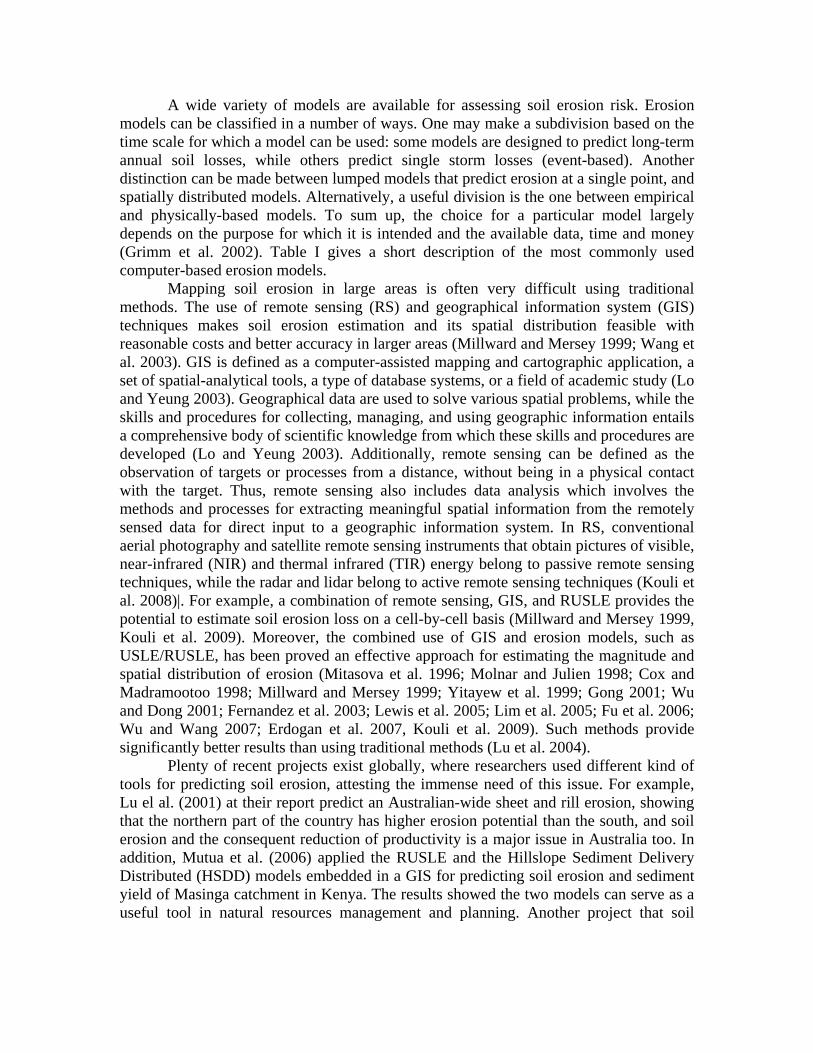
estimated to be 900 mm (Chartzoulakis et al. 2001). The study area is situated at latitudes between 35.15 and 35.50 and longitudes between 23.99 and 24.92 decimal degrees, in the western Crete Island covering the eastern part of Chania prefecture and the major part of Rethymno Prefecture (Figure 1). It comprises seven watersheds; the Kalami, Vrysses, Argyroupolis, Petres, Kourtaliotis, Prasies, and Geropotamos watersheds from west to east as shown in Figure 1. Some general geometrical characteristics of the studied watersheds are also given in Table III. The Geropotamos basin, which is located at the most eastern part of Rethymnon perfecture and covers almost 384 km2, and the Vrysses basin, which covers 190 km2, are drained by the two of the most important rivers of the region. The climate is sub-humid Mediterranean with humid and relatively cold winters and dry and warm summers.

During winter the weather is unstable due to frequent changes from low to high pressure. The annual rainfall for the broader study area has been estimated to be 665 mm. It is estimated that from the total yearly precipitation on the plains about 65% is lost to evapotranspiration, 21% as runoff to sea and only 14% goes to recharging the groundwater (Chartzoulakis et al. 2001). The rainfall is not uniformly distributed throughout the year, and it is mainly concentrated in the winter months, while the drought period covers more than six months (May to October) with evaporation values ranging from 140 mm to more than 310 mm in the peak month (Tsagarakis et al. 2004).

Figure 1. The maps show the study area in different scales. The red rectangle in the upper figure shows the broader study area. The lower figure depicts the seven (7) watersheds (shaded areas) under investigation. Table III. Morphological characteristics of the studied watersheds.

Watershed Area (sq km) Perimeter (km) Kalami 129,989 56,78 Vryses 190,017 70,96 Argyroupolis 47,925 43,09 Prasies 118,476 73,72 Petres 125,275 75,84 Geropotamos 383,544 111,93 Kourtaliotis 119,493 75,40

Regarding the geological settings, the water basins lie in an area which is mainly

composed of Miocene to Pliocene sediments which are widespread all over the study area and clastic limestones and dolomites of the Tripolis and Plattenkalk nappe which are observed mainly in the southern parts of the under investigation watersheds. Late Triasic carbonates (Tripolis nappe) and Triassic to Early Cretaceous carbonates of the Trypalion nappe are also exposed in several parts of the study area (Krahl et al. 1983) and especially in the Kalami watershed. The phyllite‐quartzite nappe covers relatively small extend and is lays on the northern part of Geropotamos basin The geological formations are broadly classified into the following hydro-lithological units: high permeability rocks which comprise the karstic limestones of Tripolis and Trypalion nappes, medium permeability rocks which consist of the Quaternary deposits as well as the Miocene to Pliocene conglomerates and marly limestones, low permeability rocks which consists of the Pliocene to Miocene marles and impervious rocks which consist of the phyllites – quartzites unit. The tectonic regime of the study area is characterizing by faults of NW-SE, NE-SW and E-W directions. These tectonic structures clearly define the boundaries between the existing geological and hydrolithological units.

Finally, the land use of the study area is mainly agricultural (up to 30%), urban fabric and bare rocks coverage is up to 5% while the natural vegetation which is mainly characterized as scrub and/or herbaceous vegetation associations (Corine Land Cover map 2000 (CLC2000 100m, version 1) of the European Environment Agency (©EEA, Copenhagen, 2000; http://www.eea.europa.eu) covers an area of almost 122000 ha (65% of the whole area).

The extensive tectonic fragmentation and the repeated thrusts, the intense morphological relief with the steep slopes, the dense drainage network with the deep valleys, the extensive human activities with the relatively dense road network, and the arable-pasture areas are some of the factors which constitute the study area particularly prone to extended soil washout in case of intense rainfall events. Data

Five thematic layers of the RUSLE factors were achieved through Geographic Information Systems and Remote Sensing methods and techniques. In addition, data of rainfall erosivity were obtained through a statistical calculation of the total amount of all the rainfalls (50 rainfall gauges) of an average period of about 21 years.

The different types of datasets used for the annual soil loss analysis of the area under investigation were as follows:

1. Geological and hydrolithological maps of the Institute of Geology and Mineral Exploration (IGME) representing lithological and structural units at 1:50000 scale.

2. Topographic maps of the Hellenic Military Geographical Service at a scale of 1:50000 to form a detailed base map with 20-m contour interval.

3. Satellite sensor data and in particular, a Landsat-ETM image acquired on 2000-07-30 with a spatial resolution of 30 m for the multi-spectral bands (6 bands) and 15 m for the panchromatic image.

4. The Corine Land Cover map 2000 (CLC2000 100 m, version 1) of the European Environment Agency (EEA, Copenhagen, 2000; http://www.eea.europa.eu). This map has a resolution of 100 m and uses 10 land use categories of Level 1 for the study area.

5. The soil map provided by the Soil Geographical Data Base of Europe at a scale of 1:1000000 (http://eusoils.jrc.it).

6. Precipitation data covering a time period of 25 years. 7. Chemical analysis data from 22 boreholes and 2 springs located inside

Geropotamos watershed. In order to create the appropriate information platform upon which to proceed in a

systematic way toward applying the RUSLE model, all available data in the form of maps were used as the basis for the creation of GIS thematic layers. The data pre-processing involved in their implementation into ArcGIS Desktop 9.1 software environment. The several maps were geo-referenced to the local projection system of Greece (GGRS ’87-Greek Geodetic Reference System), so that they could all be tied to the same projection system, together with all future information that may become available. In the next pre-processing phase, digitization of all the relevant data maps, namely geological, hydrolithological and topographical was carried out.

Data layers preparation After the creation of the primary layers, various advanced GIS techniques, such as

aggregation, measurement, overlay, logical operations, vector to raster conversion, reclassification, and map algebra were applied for data analysis Aggregation helps the user in interpreting the data, classification allows the user to classify areas within a map, and measurement can be used to determine the size of any area. The overlay function allows the user to "stack" map layers on one another. Map algebra utilities allow the user to specify mathematical relationships between map layers.

The Digital Elevation Model (DEM) of the study area with a cell size of 20 m is a continuous raster layer, in which data values represent elevation. It was generated from the digitization of the topographic maps of the study area. As a result, significant geomorphological parameters and terrain attributes such as slope gradient, hillshade, elevation values, drainage basin areas and stream networks were derived from further processing of the DEM. Hydrologic analysis was accomplished exclusively in ArcGIS Spatial Analyst, using the hydrologic tools. These tools were applied in sequence to extract hydrologic information from the DEM. We were allowed to identify and fill sinks, determine the flow direction, calculate the flow accumulation, order the segments in the drainage networks (Strahler ordering), delineate the watersheds, and finally, extract the stream network.

Remote sensing with its advantages of spatial, spectral and temporal availability of data covering large and inaccessible areas within short time has become a very important tool (Chowdhary et al. 2003). Numerous techniques can be applied depending on the desired information such as vegetation indices and classification algorithms for land-use and geological maps, soil indices for soil maps.

Once the required satellite images are purchased in digital form, the next step is to process the images for extracting the desired spatial and thematic information; satellite images without processing are not of much use, especially for scientific studies. This complex processing is done with the help of a computer by using image processing software packages known as digital image processing (Lillesand and Kiefer 2000). Several operations are needed for extracting the required data and/or information.

In a first pre-processing step, the satellite image was geocoded, using the correspondent topographic maps of the study area. After that, the Normalized Difference Vegetation Index was calculated. Generally, “indices are used extensively in vegetation analysis to bring out small differences between various vegetation types. In many cases, judiciously chosen indices can highlight and enhance differences that cannot be observed in the display of the original color bands. Indices can also be used to minimize shadow effects in satellite and aircraft multispectral images. Black and white images of individual indices or a color combination of three ratios may be generated” (Erdas Field Guide 2005). The derived NDVI layer was then implemented in a GIS environment.

All the aforementioned layers were resampled using the Nearest Neighbor method in order to create layers with 20 meters spatial resolution.

The results that were obtained on the basis of soil loss prediction were integrated with the geological, tectonic, hydrolithological structures of the drainage basins is order to reveal the role of structural and geological factors in the annual soil loss of the river basins of the study areas.

The following sections describe the estimation of the R, K, C, and LS factors from rainfall data, available soil maps, digital processing of satellite images (with the use of NDVI), and digital elevation model (DEM), respectively. Soil erosion prediction

The raster data model is a field-based approach for representing real-world features and is best employed to represent continuous geographic phenomena. This model is characterized by sub-dividing a geographic space into grid cells with values being assigned to each cell. The linear dimensions of each cell define the spatial resolution of the data, which is determined by the size of the smallest object in the geographic space to be represented. This size is also known as the “minimum mapping unit (MMU)”. In raster data models, each cell is usually restricted to a single value. Hence, multiple layers are needed to represent the spatial distribution of a number of parameters (variables). A raster-based GIS has advantages over a vector-based GIS because virtually all types of data including attribute data, image data, scanned maps, and digital terrain models can be represented in raster form (Van Der Laan 1992). Also, the vector data model is conceptually more complex and more technically difficult to implement than the raster data model. In a raster GIS, the mean annual soil erosion is calculated at a cell level as the product of six factors

Ai = RiKiLiSiCiPi (12) where the subscript i represents the ith cell.

The FF index (Eq. 5) approach was used to determine the rainfall erosivity factor and consequently the erosion risk for Central and Western Crete Island in Greece and the analysis carried out using 50 recording raingauges, showed that R is linearly correlated to FF and R is better correlated to FF than P (Aronica and Ferro 1997). This last result can be justified given that P is a robust estimator of the R factor for regions where high rainfall erosivity corresponds to high annual rainfall. For regions, such as Crete, where intensity indices (Ferro et al. 1991) are required for soil erosion studies, FF is a better estimator of the R factor because FF takes into account the rainfall seasonal distribution.

Rainfall erosivity factor (R)

The basis for this climatological analysis which will be used for soil risk analysis is a data set of monthly rain-gauge observations with high spatial resolution over most of the region covered the western and central part of Crete Island. It was established by combining several sectorial data sets that have been archived by governmental services and hydrological agencies of the Crete Region. Our aim was to make the best possible use of all available existing networks. Upon request, most of the data centres that were contacted have kindly provided an extensive portion of their data for our research.

The precipitation data set

Table IV lists the individual data sets and indicate the name of the station, longitude/latitude and elevation of the station, the length of records in years, the network where the station belongs and some calculated parameters which are going to comment in later section. Originally our requests were made for all the available data independent the time periods. An optimal coverage in the combined data set was achieved, which was

then chosen as the reference period. The spatial distribution of rain-gauge stations from which observations are available is shown in Figure (2). For our research, data obtained from three different agencies; the Department of Hydrology and Water Resources - Crete Region (DHWR-CR), the National Agricultural Research Foundation located in Chania in Crete Island (NAGREF) and the Branch of the Institute of Geology and Mineral Exploration situated in Rethymnon in Crete Island (IGME).

There is still considerable inhomogeneity in the spatial coverage across the domain and this will be accounted for by using an analysis scheme with a regionally variable spatial resolution. During the interpretation of the climatological results it will be important to keep in mind the variable density of the observational basis.

Figure 2. A map of the western (Chania Prefecture) and central (Rethymon Prefecture) Crete Island showing the location/spatial distribution of the fifty meteorological (raingauges) stations used for our research.

The data sets obtained from the above mentioned data centers exhibit variable quality status. In order to have the complete control of the data procedure, the raw data were requested from the data providers. In most of the cases, the poor data quality of the precipitation reports was due to typing, transmission and coding errors. Again our own experience shows that the declaration of missing observations is not handled properly everywhere. In some of the original data sets, time series with dry reports over several

Quality control

months have been detected, which apparently should have been indicated as measurement failure.

In order to exclude the most obvious errors from the precipitation data set in the study area, a quality control procedure was applied to all the monthly observations prior to their spatial analysis. For this purpose, a simple range test and a spatial consistency test was applied to the data set. Daily reports queried by the quality testing were then simply dropped and no attempt was made to estimate appropriate replacements.

The range test filters from the data set reports larger than an upper limit of 700 mm per month. Although observations exceeding such an amount have been observed in the Askyfou region (Chania Perfecture) in extreme cases, their numerous occurrences in the data set are mostly bogus reports due to typing errors. For the spatial consistency testing we adopted, with modifications, a procedure that is operational at the Greek Weather Service. Each monthly report is verified against some tolerance bounds derived from neighboring stations. These tolerance bounds depend upon both the long-term monthly mean at the stations under consideration. The consideration of monthly means allows systematic anomalies to be taken into account, for example, exposure of the stations. The tolerance bounds used in our study also depend upon the proximity of surrounding observations, in order to cope with the variable network density. The testing procedure deals separately with cases of isolated precipitation surrounded by dry reports, and cases of isolated dryness surrounded by rainy reports. The rejection rate after the quality control was less than 0.5% for the data sets. Thus, there is no significant reduction in the data amount.

Based on the suggested methodology as reported above and using equations (3), (4) and (5), the modified Fournier index (MFI) was estimated for all the rainfall gauges (Table I, column 8th). In order to estimate the most appropriate R-factor using the calculated MFI, the following two R-MFI relationships as suggested by the Ferro et al. (1999) and Renard and Freimund (1994) for the regions of Sicily-Italy and the Morocco, respectively were used,

R-factor estimation

56.16120.0 MFIR ⋅= - Sicily – Italy (13) 50.1264.0 MFIR ⋅= - Morocco (14)

The R-factor for each of the relationships (13) and (14) was estimated and the mean value of the resulted R-factor was finally adopted as is shown in Table I (column 10). Table IV. Characteristics of the Western and Central Crete raingauge stations used to derive the rainfall erosivity factor. MFI is the estimated modified fournier index, the R-factor for the areas of Sicily and Morocco were also estimated in order to use the average of these values. STATIONS x y z years Network MFI R_factor R_factor mean R Stroblo 470182 3913677 2 DHWR-CR 220,06 2761,31 1469,01 2115,16 Askyfou 516466 3905923 740 46 DHWR-CR 325,35 5081,81 2640,82 3861,32 Kournas Lake 524791 3909942 2 DHWR-CR 238,26 3125,73 1654,97 2390,35 Vamos 517955 3918865 2 42 DHWR-CR 127,82 1183,16 650,29 916,72 Chania 502820 3928090 62 52 DHWR-CR 85,36 630,28 354,91 492,60

Kalybes 514922 3922556 24 33 DHWR-CR 103,79 854,98 475,82 665,40 Mouri 510690 3899678 24 43 DHWR-CR 156,46 1621,89 880,68 1251,28 PaleaRoumata 480122 3917020 316 46 DHWR-CR 200,16 2381,79 1274,33 1828,06 Palaioxora 470982 3898560 48 26 DHWR-CR 90,98 696,11 390,49 543,30 Prasses 485374 3914558 520 16 DHWR-CR 285,28 4139,76 2168,30 3154,03 Souda 510372 3933641 152 42 DHWR-CR 88,63 668,36 375,50 521,93 Kandanos 476225 3909024 3 DHWR-CR 234,21 3043,24 1612,95 2328,09 Gadvos 506273 3856016 10 17 DHWR-CR 51,78 288,96 167,67 228,32 Meskla 495828 3917564 4 DHWR-CR 223,54 2829,73 1503,99 2166,86 Tavronitis 483600 3931738 15 35 NAGREF 98,56 788,75 440,33 614,54 ChaniaAgroki 504069 3927522 8 35 NAGREF 101,93 831,13 463,06 647,09 Drapanias 472991 3927382 29 19 NAGREF 109,32 927,06 514,34 720,70 Alikianos 491672 3923277 19 NAGREF 120,69 1081,77 596,62 839,20 Kandanos 476234 3908989 158 19 NAGREF 150,18 1521,53 828,22 1174,87 Koundoura 467146 3899182 59 9 NAGREF 72,49 488,44 277,75 383,10 Fragkokastello 520981 3892981 5 NAGREF 102,80 842,24 469,01 655,63 Falasarna 461635 3925886 12 NAGREF 94,88 743,26 415,89 579,58 Zymbragou 477730 3921328 235 19 NAGREF 155,51 1606,48 872,63 1239,56 Armenoi 514222 3920407 50 12 NAGREF 121,53 1093,62 602,90 848,26 Patsianos 521045 3895375 5 NAGREF 148,77 1499,21 816,53 1157,87 Anopolis 506878 3897748 600 12 IGME 135,78 1300,10 711,98 1006,04 Askyfou 516943 3905950 700 21 IGME 317,83 4899,77 2549,79 3724,78 Alikampos 519154 3911481 330 12 IGME 188,21 2163,75 1161,96 1662,85 Rodopou 477398 3934154 230 9 IGME 138,01 1333,60 729,61 1031,61 Epanoxori 484531 3908658 600 11 IGME 174,85 1928,90 1040,43 1484,66 Rogdia 467152 3915404 580 8 IGME 172,91 1895,65 1023,17 1459,41 Floria 475561 3914830 600 8 IGME 238,76 3136,05 1660,22 2398,14 Omalos 491146 3910915 1050 7 IGME 257,70 3532,60 1861,61 2697,10 Sirikari 466975 3919688 450 8 IGME 210,64 2579,21 1375,73 1977,47 Koystogerako 485010 3903952 530 12 IGME 164,36 1751,49 948,24 1349,87 Xasi(Boutas) 467500 3904906 370 14 IGME 122,97 1113,84 613,62 863,73 Prasses 486150 3914812 520 12 IGME 274,79 3904,66 2049,77 2977,21 Therissos 498286 3917629 580 21 IGME 194,51 2277,78 1220,78 1749,28 Melidoni 510334 3915922 400 21 IGME 198,40 2349,18 1257,55 1803,37 Kampoi 506136 3919063 560 12 IGME 211,71 2599,53 1386,16 1992,84 Spili 548679 3899338 390 34 DHWR-CR 176,99 1965,85 1059,58 1512,72 Melampes 559367 3888311 560 35 DHWR-CR 123,72 1124,50 619,26 871,88 Leykogeia 541121 3893756 90 32 DHWR-CR 127,08 1172,50 644,66 908,58 Kabousi 554689 3908615 580 29 DHWR-CR 129,05 1200,97 659,70 930,34 Gerakari 556273 3897534 580 31 DHWR-CR 204,36 2460,19 1314,64 1887,42 Garazo 572839 3912440 260 3 DHWR-CR 257,51 3528,50 1859,53 2694,02 Byzari 563871 3895736 310 29 DHWR-CR 118,26 1048,04 578,72 813,38 Boleones 553207 3903061 260 33 DHWR-CR 177,70 1978,17 1065,97 1522,07 Anogeia 580477 3905111 740 74 DHWR-CR 152,03 1550,82 843,54 1197,18 Agia Galini 562429 3884635 20 30 DHWR-CR 94,29 736,07 412,01 574,04

The calculated rainfall erosivity factors were interpolated with geostatistical as well as deterministic techniques. After applying and testing several geospatial prediction techniques the Ordinary Kriging (OK) interpolator was chosen for interpolating the point

Cross Validation

information (R-factor). Compared with the rest of interpolation methods, OK gave the best cross validation results and root mean squared (RMS) errors. RMS is given by the equation:

2

1

( )ni p io

i

DI DIRMS

n=

−=∑

(15)

where i pDI is the predicted value for site i, ioDI is the observed value for site i, and n the total number of sites.

“Kriging is a moderately quick interpolator that can be exact or smoothed depending on the measurement error model. “Instead of weighting nearby data points by some power of their inverted distance, ordinary kriging relies on the spatial correlation structure of the data to determine the weighting values. This is a more rigorous approach to modelling, as correlation between data points determines the estimated value at an unsampled point. Furthermore, ordinary kriging makes the assumption of normality among the data points” (Isaaks & Srivastava 1989).

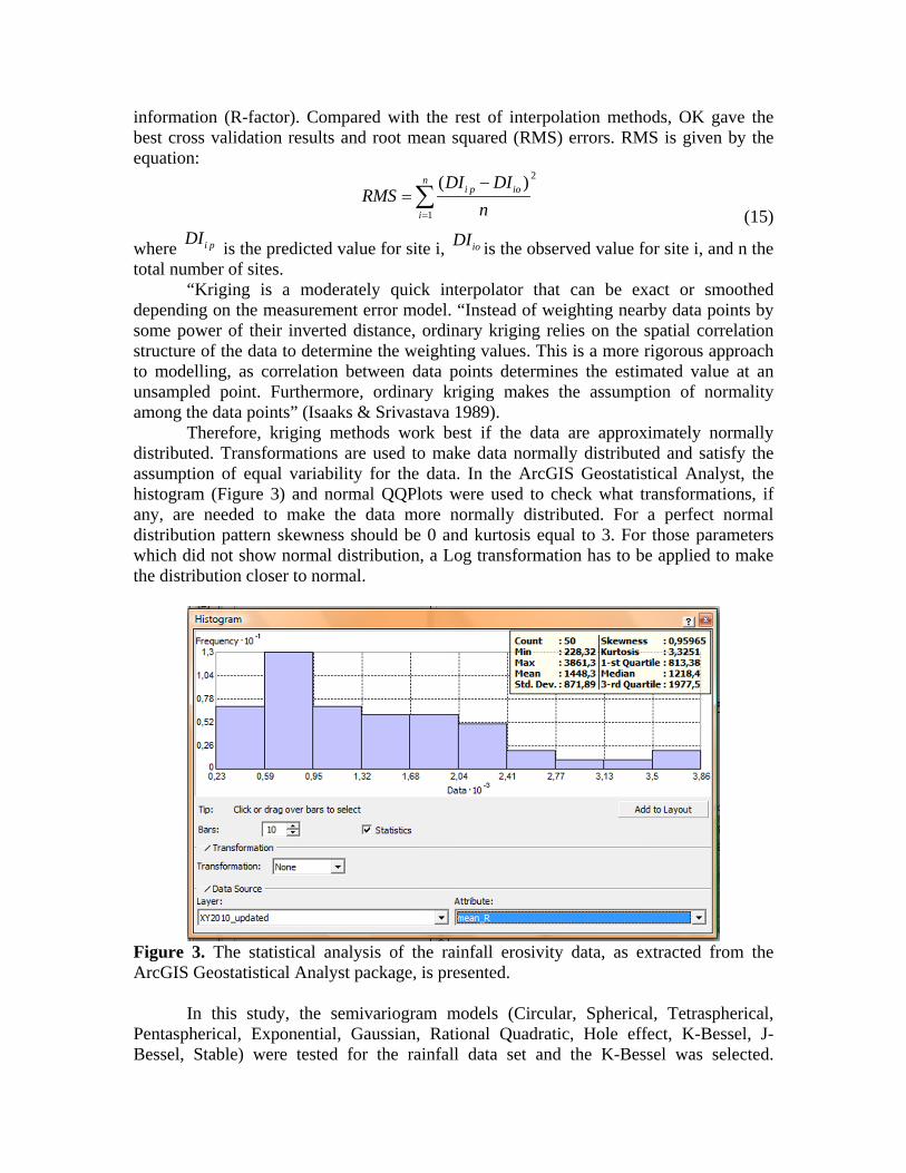
Therefore, kriging methods work best if the data are approximately normally distributed. Transformations are used to make data normally distributed and satisfy the assumption of equal variability for the data. In the ArcGIS Geostatistical Analyst, the histogram (Figure 3) and normal QQPlots were used to check what transformations, if any, are needed to make the data more normally distributed. For a perfect normal distribution pattern skewness should be 0 and kurtosis equal to 3. For those parameters which did not show normal distribution, a Log transformation has to be applied to make the distribution closer to normal.

Figure 3. The statistical analysis of the rainfall erosivity data, as extracted from the ArcGIS Geostatistical Analyst package, is presented.

In this study, the semivariogram models (Circular, Spherical, Tetraspherical, Pentaspherical, Exponential, Gaussian, Rational Quadratic, Hole effect, K-Bessel, J-Bessel, Stable) were tested for the rainfall data set and the K-Bessel was selected.

Prediction performances were assessed by cross-validation. Cross-validation allows determination of which model provides the best predictions. It uses all of the data to estimate the trend. Then it removes each data location, one at a time, and predicts the associated data value. The predicted and actual values at the location of the omitted point are compared. For all points, cross-validation compares the measured and predicted values. Generally, the best model is the one that has the mean nearest to zero and the smallest root-mean-squared prediction error. If the prediction errors are unbiased, the mean prediction error should be near zero but we should have always in mind that this value depends on the scale of the data. Table V, presents the cross validation results of the estimated R-factor. For the standardized error estimation, the measured values are subtracted from the predicted values and then divided by the estimated standard errors.

Figure (4) shows the plot of the predicted versus the estimated R-factors. Details on the prediction errors, such as, the mean value (71.57), the root mean square (rms) (586.1), the average standard error (795.1), the mean standardized error (0.05884) and the standardized rms (0.8714) are given.

Generally, if the average standard errors are close to the root-mean-squared prediction errors, then the variability in prediction is well estimated. If the average standard errors are greater than the root-mean-squared prediction errors, then the variability of the predictions is overestimated; if the average standard errors are less than the root-mean-squared prediction errors, then the variability in the prediction is underestimated. Another way to look at this is to divide each prediction error by its estimated prediction standard error. They should be similar, on average, and so the root-mean-squared standardized errors should be close to 1 if the prediction standard errors are valid. If the root-mean-squared standardized errors are greater than 1, the variability in our predictions is underestimated; while if the root-mean-squared standardized errors are less than 1, then the variability in predictions is overestimated (ESRI ArcGIS Desktop Help 2004). Table V. CrossValidation of the estimated R-factor was used for verifying our results. The Ordinary Kriging Geostatistical interpolator was selected. Station Measured Predicted Error StdError Stdd_Error NormValue Included

Stroblo 2115,16 1766,2 -348,9 592,2 -0,59 -0,74 Yes

Askyfou 3861,32 2593,4 -1267,9 616,9 -2,06 -2,33 Yes

Kournas Lake 2390,35 2188,3 -202,0 795,8 -0,25 -0,67 Yes

Vamos 916,72 1088,7 171,9 635,6 0,27 0,18 Yes

Chania 492,60 694,5 201,9 660,4 0,31 0,33 Yes

Kalybes 665,40 612,0 -53,4 632,3 -0,08 -0,44 Yes

Mouri 1251,28 1989,1 737,9 651,7 1,13 1,48 Yes

PaleaRoumata 1828,06 2256,7 428,7 592,6 0,72 0,95 Yes

Palaioxora 543,30 688,4 145,1 705,3 0,21 0,03 Yes

Prasses 3154,03 2243,0 -911,1 587,1 -1,55 -1,48 Yes

Souda 521,93 660,8 138,9 863,7 0,16 -0,18 Yes

Kandanos 2328,09 1458,0 -870,1 600,4 -1,45 -1,34 Yes

Gadvos 228,32 876,1 647,8 1031,4 0,63 0,67 Yes

Meskla 2166,86 2031,2 -135,6 615,2 -0,22 -0,55 Yes

Tavronitis 614,54 797,9 183,4 777,9 0,24 0,13 Yes

ChaniaAgrokip 647,09 658,7 11,6 635,9 0,02 -0,33 Yes

Drapanias 720,70 924,7 204,0 706,1 0,29 0,23 Yes

Alikianos 839,20 1597,9 758,7 715,1 1,06 1,34 Yes

Kandanos 1174,87 1859,9 685,1 602,2 1,14 1,64 Yes

Koundoura 383,10 599,2 216,1 684,9 0,32 0,39 Yes

Fragkokastello 655,63 942,9 287,3 702,0 0,41 0,55 Yes

Falasarna 579,58 1408,0 828,4 920,8 0,90 1,23 Yes

Zymbragou 1239,56 1725,3 485,7 633,6 0,77 1,04 Yes

Armenoi 848,26 973,0 124,7 595,4 0,21 0,08 Yes

Patsianos 1157,87 1376,3 218,4 674,9 0,32 0,44 Yes

Anopolis 1006,04 1135,6 129,6 767,0 0,17 -0,08 Yes

Askyfou 3724,78 2669,5 -1055,3 615,2 -1,72 -1,88 Yes

Alikampos 1662,85 2776,7 1113,9 609,3 1,83 2,33 Yes

Rodopou 1031,61 857,6 -174,0 770,9 -0,23 -0,61 Yes

Epanoxori 1484,66 2397,5 912,8 595,6 1,53 1,88 Yes

Rogdia 1459,41 1893,5 434,1 634,0 0,68 0,88 Yes

Floria 2398,14 2034,2 -364,0 580,6 -0,63 -0,81 Yes

Omalos 2697,10 2248,6 -448,5 664,5 -0,67 -0,88 Yes

Sirikari 1977,47 1207,6 -769,9 631,5 -1,22 -1,13 Yes

Koystogerako 1349,87 1568,7 218,8 755,0 0,29 0,28 Yes

Xasi(Boutas) 863,73 973,1 109,4 675,6 0,16 -0,13 Yes

Prasses 2977,21 2359,8 -617,4 590,4 -1,05 -1,04 Yes

Therissos 1749,28 2046,5 297,2 623,5 0,48 0,61 Yes

Melidoni 1803,37 1831,5 28,2 647,6 0,04 -0,28 Yes

Kampoi 1992,84 1225,3 -767,6 624,5 -1,23 -1,23 Yes

Spili 1512,72 1501,8 -10,9 698,4 -0,02 -0,39 Yes

Melampes 871,88 999,0 127,1 690,8 0,18 -0,03 Yes

Leykogeia 908,58 1267,8 359,2 946,6 0,38 0,50 Yes

Kabousi 930,34 1573,6 643,3 807,2 0,80 1,13 Yes

Gerakari 1887,42 1238,4 -649,0 667,5 -0,97 -0,95 Yes

Garazo 2694,02 1027,4 -1666,6 988,6 -1,69 -1,64 Yes

Byzari 813,38 1345,2 531,8 828,0 0,64 0,81 Yes

Boleones 1522,07 1417,6 -104,4 630,4 -0,17 -0,50 Yes

Anogeia 1197,18 1824,2 627,0 980,0 0,64 0,74 Yes

Agia Galini 574,04 693,4 119,4 774,1 0,15 -0,23 Yes

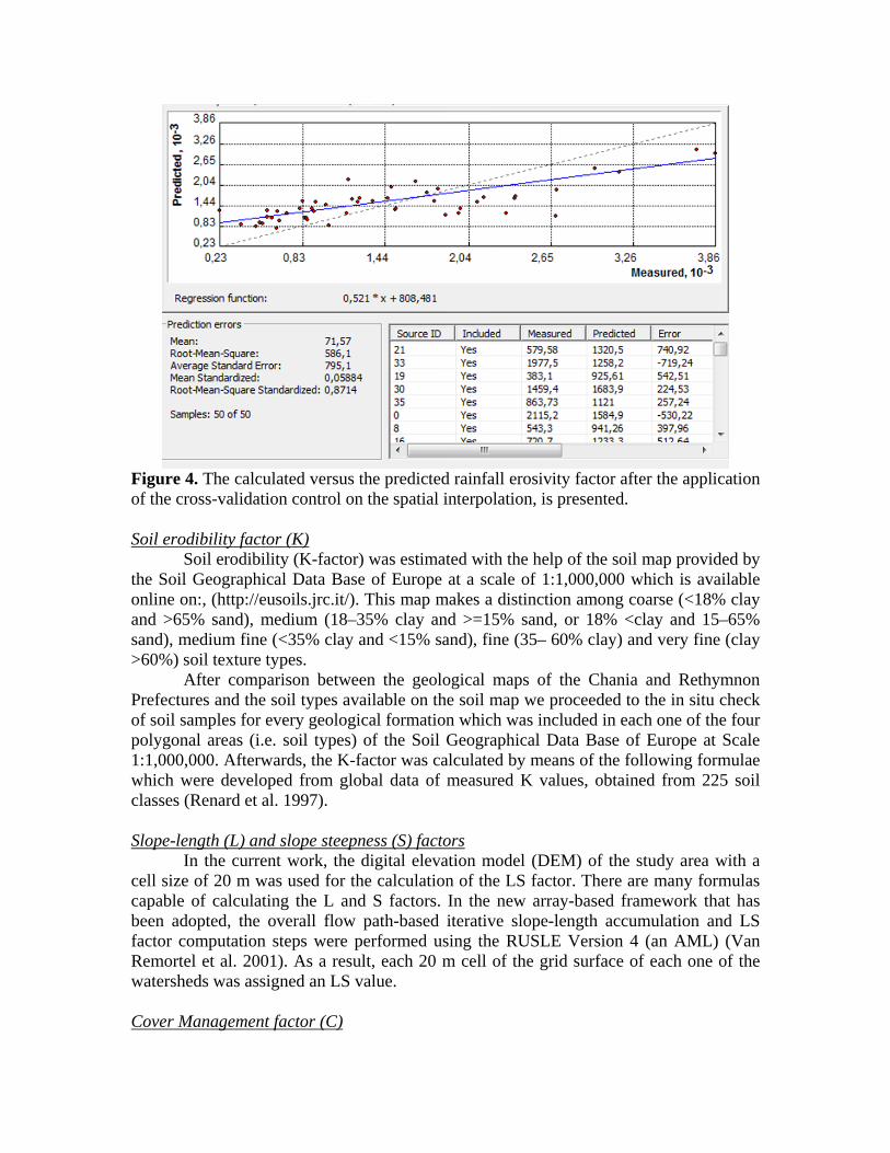
Figure 4. The calculated versus the predicted rainfall erosivity factor after the application of the cross-validation control on the spatial interpolation, is presented.

Soil erodibility (K-factor) was estimated with the help of the soil map provided by the Soil Geographical Data Base of Europe at a scale of 1:1,000,000 which is available online on:, (http://eusoils.jrc.it/). This map makes a distinction among coarse (<18% clay and >65% sand), medium (18–35% clay and >=15% sand, or 18% <clay and 15–65% sand), medium fine (<35% clay and <15% sand), fine (35– 60% clay) and very fine (clay >60%) soil texture types.

Soil erodibility factor (K)

After comparison between the geological maps of the Chania and Rethymnon Prefectures and the soil types available on the soil map we proceeded to the in situ check of soil samples for every geological formation which was included in each one of the four polygonal areas (i.e. soil types) of the Soil Geographical Data Base of Europe at Scale 1:1,000,000. Afterwards, the K-factor was calculated by means of the following formulae which were developed from global data of measured K values, obtained from 225 soil classes (Renard et al. 1997).

In the current work, the digital elevation model (DEM) of the study area with a cell size of 20 m was used for the calculation of the LS factor. There are many formulas capable of calculating the L and S factors. In the new array-based framework that has been adopted, the overall flow path-based iterative slope-length accumulation and LS factor computation steps were performed using the RUSLE Version 4 (an AML) (Van Remortel et al. 2001). As a result, each 20 m cell of the grid surface of each one of the watersheds was assigned an LS value.

Slope-length (L) and slope steepness (S) factors

Cover Management factor (C)

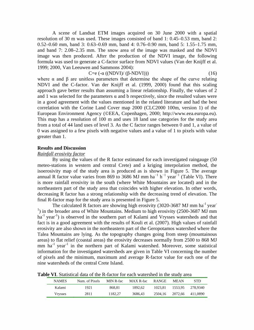
A scene of Landsat ETM images acquired on 30 June 2000 with a spatial resolution of 30 m was used. These images consisted of band 1: 0.45–0.53 mm, band 2: 0.52–0.60 mm, band 3: 0.63–0.69 mm, band 4: 0.76–0.90 mm, band 5: 1.55–1.75 mm, and band 7: 2.08–2.35 mm. The snow area of the image was masked and the NDVI image was then produced. After the production of the NDVI image, the following formula was used to generate a C-factor surface from NDVI values (Van der Knijff et al. 1999; 2000, Van Leeuwen and Sammons 2004):

C=e (-α ((NDVI)/ (β-NDVI))) (16) where α and β are unitless parameters that determine the shape of the curve relating NDVI and the C-factor. Van der Knijff et al. (1999, 2000) found that this scaling approach gave better results than assuming a linear relationship. Finally, the values of 2 and 1 was selected for the parameters α and b respectively, since the resulted values were in a good agreement with the values mentioned in the related literature and had the best correlation with the Corine Land Cover map 2000 (CLC2000 100m, version 1) of the European Environment Agency (©EEA, Copenhagen, 2000; http://www.eea.europa.eu). This map has a resolution of 100 m and uses 18 land use categories for the study area from a total of 44 land uses of level 3. As the C factor ranges between 0 and 1, a value of 0 was assigned to a few pixels with negative values and a value of 1 to pixels with value greater than 1. Results and Discussion

By using the values of the R factor estimated for each investigated raingauge (50 meteo-stations in western and central Crete) and a kriging interpolation method, the isoerosivity map of the study area is produced as is shown in Figure 5. The average annual R factor value varies from 869 to 3686 MJ mm ha−1 h−1 year−1 (Table VI). There is more rainfall erosivity in the south (where White Mountains are located) and in the northeastern part of the study area that coincides with higher elevation. In other words, decreasing R factor has a strong relationship with the decreasing trend of elevation. The final R-factor map for the study area is presented in Figure 5.

Rainfall erosivity factor

The calculated R factors are showing high erosivity (3020-3687 MJ mm ha-1 year-

1) in the broader area of White Mountains. Medium to high erosivity (2500-3687 MJ mm ha-1 year-1) is observed in the southern part of Kalami and Vrysses watersheds and that fact is in a good agreement with the results of Kouli et al. (2007). High values of rainfall erosivity are also shown in the northeastern part of the Geropotamos watershed where the Talea Mountains are lying. As the topography changes going from steep (mountainous areas) to flat relief (coastal areas) the erosivity decreases normally from 2500 to 868 MJ mm ha-1 year-1 in the northern part of Kalami watershed. Moreover, some statistical information for the investigated watersheds are given in Table VI concerning the number of pixels and the minimum, maximum and average R-factor value for each one of the nine watersheds of the central Crete Island. Table VI. Statistical data of the R-factor for each watershed in the study area

NAMES Num. of Pixels MIN R-fac MAX R-fac RANGE MEAN STD

Kalami 1921 868,81 1892,62 1023,81 1553,95 278,9340

Vrysses 2811 1182,27 3686,43 2504,16 2072,66 411,0890

Argyroupolis 712 1530,75 2240,06 709,31 1807,42 143,1750

Prasies 1740 1305,27 1553,43 248,16 1415,92 51,3157

Petres 1842 1359,39 1703,05 343,65 1486,93 86,1969

Geropotamos 5310 1244,01 2476,03 1232,02 1598,01 215,9990

Kourtaliotis 1758 982,17 1487,17 505,00 1295,87 94,4434

Figure 5. The spatial distribution of the calculated R-factor (in grid surface) of the western and central part of the Crete Island is shown.

The K-factor was calculated through the mean values of grain size analysis from various measurements acquired on Crete. Soil erodibility values range from 0.02 t h MJ−1 mm−1 in large areas in the southern part of the study area (sandy soils) to 0.035 and 0.04 t h MJ−1 mm−1 for the loamy and silt loamy soils, in the central/southern and northern parts of the under investigation watersheds, respectively (Fig. 6). The highest values of the soil erodibility factor are spatially well correlated with the areas which expose quaternary and neogene sediments.

Soil Erodibility factor

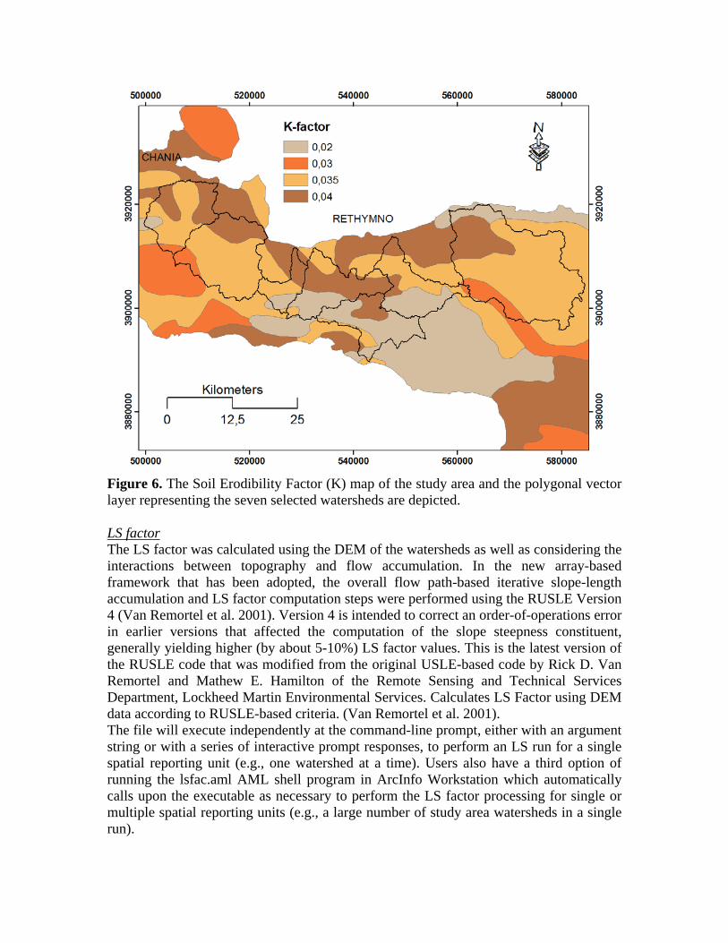
Figure 6. The Soil Erodibility Factor (K) map of the study area and the polygonal vector layer representing the seven selected watersheds are depicted.

The LS factor was calculated using the DEM of the watersheds as well as considering the interactions between topography and flow accumulation. In the new array-based framework that has been adopted, the overall flow path-based iterative slope-length accumulation and LS factor computation steps were performed using the RUSLE Version 4 (Van Remortel et al. 2001). Version 4 is intended to correct an order-of-operations error in earlier versions that affected the computation of the slope steepness constituent, generally yielding higher (by about 5-10%) LS factor values. This is the latest version of the RUSLE code that was modified from the original USLE-based code by Rick D. Van Remortel and Mathew E. Hamilton of the Remote Sensing and Technical Services Department, Lockheed Martin Environmental Services. Calculates LS Factor using DEM data according to RUSLE-based criteria. (Van Remortel et al. 2001).

LS factor

The file will execute independently at the command-line prompt, either with an argument string or with a series of interactive prompt responses, to perform an LS run for a single spatial reporting unit (e.g., one watershed at a time). Users also have a third option of running the lsfac.aml AML shell program in ArcInfo Workstation which automatically calls upon the executable as necessary to perform the LS factor processing for single or multiple spatial reporting units (e.g., a large number of study area watersheds in a single run).

It can be seen that the LS factor varies from 0 to 148. However, some specific areas with steep slopes (such as along the rivers) have greater LS values. Figure 7 shows the LS-factor grid maps of the study watersheds.

The Vrysses watershed shows the greatest LS factor among the seven studied watersheds (Table VII). The topographic factor ranges from 0 in the flat zones to 148 at the steep slopes in the southern part of the basin. Although Kalami basin is characterized by the greatest elevation drop of 2187 m and consequently the greatest LS factor, the great values are present in a limited part of the basin (Fig. 6). On the other hand, Argyroupolis watershed shows maximum LS factor equal to 118 but its mean value is significantly greater than this of Vrysses basin (Fig. 6). This fact implies extended areas of steep slopes which are prone to severe erosion. In the opposite hand, Petres watershed is characterized by relatively small LS factor values and this is consistent with its relatively low elevation values and the smallest extent of the watershed (Figure 7). It is noteworthy, the fact that despite its relatively low maximum LS value (i.e. 93), Prasies basin shows high mean LS factor values of 110 and 7.88 in comparison with the Geropotamos and especially Kourtaliotis watersheds. Table VII. Statistical data of the LS-factor for each watershed in the study area

Watersheds Min Max Mean Std Kalami 0 117 7.65 8.69 Vrysses 0 148 8.52 9.37 Argyroupolis 0 118 9.36 9.28 Prasies 0 93 7.88 8.05 Petres 0 99 5.62 6.78 Geropotamos 0 111 6.68 7.72 Kourtaliotis 0 121 6.80 7.75

Figure 7. The LS maps as calculated from the processing of DEM of the seven selected watersheds.

The C factor map was prepared based on NDVI (Figure 8) applying the NDVI-C relationship proposed by Van der Knijff et al. (1999, 2000). In general, this factor has completely inverse relationship with NDVI. As seen from the Figure 9, the greatest amount of this parameter coincides with the urban areas along the coastline in the northern part of the island (magenta color) whereas the least amount is related to the area with dense forest vegetation (deep green color).

Cover Management factor

The NDVI thematic map resulted from the Landsat-ETM satellite image of the study area showing a range from -0.32 to 0.85 (Figure 8). The Corine Land Cover vector map was overlain to the pixel by pixel estimated cover management factor grid (Fig. 8) and the mean C value for every Corine class was calculated (Table VI). As a result, the mean C values range inside the watersheds from 0.13 for the forest class to 0.785 for the bare rocks class (Table VIII). The C-values for forest are near 0 and for the bare rocks tending to 1 which looks realistic. The predicted C-values of the arable classes depend on crop type and management practices.

The approach followed here it was based to the available data. To improve the results, satellite images with better geometric and spectral characteristics can provide detailed information, as well as field measurements can be proved efficient in order to relate biophysical properties (like the C-factor) to remotely-sensed data. Table VIII The average C factor values for the several land uses of the study area (Kouli et al. 2009).

Land Use Mean Broad-leaved forest 0.130266 Fruit trees and berry plantations 0.178411 Mixed forest 0.182351 Vineyards 0.294141 Olive groves 0.304188 Land principally occupied by agriculture 0.307676 Coniferous forest 0.338087 Transitional woodland-shrub 0.375549 Sclerophyllous vegetation 0.412805 Complex cultivation patterns 0.428191 Non-irrigated arable land 0.496456 Moors and heathland 0.500111 Pastures 0.543197 Natural grasslands 0.545464 Construction sites 0.548493 Beaches, dunes, sands 0.575484 Sparsely vegetated areas 0.644916 Bare rocks 0.785093

Figure 8. The NDVI thematic map resulted from the Landsat-ETM satellite image of the study area showing a range from -0.32 to 0.85.

Figure 9. The cover management factor distribution which derived from the NDVI image (Figure 8).

Soil loss values were computed by overlaying the four grid surfaces of each one of the seven catchments: the grid surface representing the R-factor values, the grid surface representing the K-factor values, the grid surface representing the C-factor values and the grid surface representing the LS-factor values in the ArcView GIS software environment.

Soil Loss and hydro-geo-tectonic parameters

Soil loss values (Table IX) range between 0 and 5134 t/ha yr for the Kalami watershed, with a mean value of 204.42 t/ha yr, between 0 and 5760 t/ha yr with a mean value of 335.66 t/ha yr for the Vrysses watershed, between 0 and 4545.96 t/ha yr for Argyroupolis basin with a mean value of 269.49 t/ha yr, between 0 and 1920.58 t/ha yr for the Prasies basin (mean value equal to 108.58 t/ha yr), between 0 and 3149.26 t/ha yr for the Petres watershed (mean value equal to 85.52 t/ha yr), between 0 and 4932.78 t/ha yr for the Geropotamos basin with a mean value of 170.06 t/ha yr, between 0 and 4254 t/ha yr for the Keritis watershed (mean value equal to 193.527 t/ha yr) and between 0 to 2792.19 t/ha yr for the Kourtaliotis watershed with a mean value of 94.73 t/ha yr. The highest mean soil loss values are spatially correlated with the steepest slopes.

The resulting map for the study area can be seen in Figure 11. Soil loss values range between 0 and 5761 (t/ha-1 year-1). With regard to the spatial variation, the southwest and northeastern part of the whole study area is more prone to erosion than the southeastern, northwestern and central area. However, it should be noted that areas with amount of erosion greater than 75 ton h-1 year-1 have been distributed in the watershed non-uniformly (Figure 11). Reason for this high soil loss is related to its close relationship with high elevation and steep topography (LS factor) and high rainfall erosivity (see figure 5). Table IX. Statistical data of the estimated annual soil loss for each watershed in the study area

Watersheds Min Max Mean Std Kalami 0 5134.06 204.42 322.40 Vrysses 0 5760.67 335.66 428.82 Argyroupolis 0 4545.96 269.49 361.78 Prasies 0 1920.58 108.58 142.79 Petres 0 3149.26 85.52 132.10 Geropotamos 0 4932.78 170.06 257.96 Kourtaliotis 0 2792.19 94.73 140.20

Figure 10. Soil loss maps for each studied watershed (from west to east), after the application of the RUSLE equation are presented.

Figure 11. The soil loss map in tons/ha yr for the watersheds under investigation, after the application of the RUSLE equation, is presented.

Correlations between the tectonic characteristics which govern the geomorphic evolution of the watersheds and the calculated annual soil losses can be easily defined. Generally, the tectonic characteristics (faults and other lineaments) which are usually responsible for sedimentation and erosion processes (changes in relief and steepness) are in direct correlation with the soil losses. Figures (12a and 12b) are in an agreement with the aforementioned assumption since high soil losses are observed in the north-eastern part of Kalami and Vrysses watersheds northern the fault system directed NW-SE and into the central part (tectonic graben oriented WNW-ESE) of the Geropotamos basin, respectively.

Figure 12. The correlation between the tectonic features and the estimated annual soil loss is presented for Kalami and Vrysses watersheds (upper figure) and for Geropotamos basin (lower figure).

From the hydrolithological point of view, the geological formations composed the watersheds under investigation are classified into six hydro-lithological units (Soupios et al. 2009): a) (K1, K2) high to medium permeability rocks, which comprise the karstic limestones of Tripolis and Trypalion nappes and dolomitic rocks, b) (P1) fluctuant permeability formations which composed of recent to present alluvial deposits, eluvial mantle materials, fluvial deposits, talus cones, dunes and conglomerates in places, c) (P2) medium to low permeability formations which consists mainly of Miocene and Pliocene deposits (Neogene marly limestones and conglomerates), d) (P3) low to very low permeability formations which composed of Pliocene and Miocene marls and other impermeable Neogene formations and e) (I2) low to very low permeability formations which mainly composed of metamorphic (phyllites, etc) and rocks of all the geological units and nappes (including the Ionion nappe).

Based on the aforementioned and annotated the Table X, we can conclude that areas composed of high permeability rocks (K1 and K2) such as karstic and dolomitic limestones, present the highest soil losses (Figure 13) since the water passed through the fracture chaotic system, accelerate the erosion processes producing large quantities of terra rossa and other alluvial sediments. Consequently, a correlation between the hydrolithological characteristics of the geological formations of the studied watersheds and the soil losses is observed. Table X. The hydrolithological characteristics (permeability) in comparison with the calculated soil losses for the Kalami watershed is presented.

PERMEABILITY AREA RANGE MEAN STD SUM

I2 17240800 1356,56 127,324 141,369 2702570

K1 65792200 5134,06 274,760 374,873 22255600

K2 6249450 3490,90 504,032 445,590 3878020

P1 9313260 1068,43 28,067 70,736 321819

P2 17781800 1690,87 69,864 99,984 1529460

P3 7780540 1081,61 58,610 104,573 561429

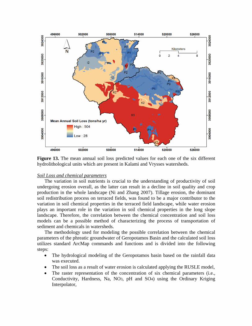
Figure 13. The mean annual soil loss predicted values for each one of the six different hydrolithological units which are present in Kalami and Vrysses watersheds.

The variation in soil nutrients is crucial to the understanding of productivity of soil undergoing erosion overall, as the latter can result in a decline in soil quality and crop production in the whole landscape (Ni and Zhang 2007). Tillage erosion, the dominant soil redistribution process on terraced fields, was found to be a major contributor to the variation in soil chemical properties in the terraced field landscape, while water erosion plays an important role in the variation in soil chemical properties in the long slope landscape. Therefore, the correlation between the chemical concentration and soil loss models can be a possible method of characterizing the process of transportation of sediment and chemicals in watersheds.

Soil Loss and chemical parameters

The methodology used for modeling the possible correlation between the chemical parameters of the phreatic groundwater of Geropotamos Basin and the calculated soil loss utilizes standard ArcMap commands and functions and is divided into the following steps:

• The hydrological modeling of the Geropotamos basin based on the rainfall data was executed.

• The soil loss as a result of water erosion is calculated applying the RUSLE model, • The raster representation of the concentration of six chemical parameters (i.e.,

Conductivity, Hardness, Na, NO3, pH and SO4) using the Ordinary Kriging Interpolator,

• Application of statistical techniques to examine possible spatial dependence between the chemical concentrations with the estimated annual soil losses for the area of Geropotamos basin (Table XI).

Table (XI) shows the cross correlation between the chemical model (six chemical parameters - conductivity, hardness, Na, NO3, SO4, pH) and the soil loss model in Geropotamos watershed. The correlation coefficient between the two models is found to be between 0.0006 and 0.2, which reflects a weak negative correlation between the two models. Table XI. The correlation matrix between annual soil loss and six selected groundwater chemical parameters Layer Soil_loss Conductivity Hardness Na NO3 pH SO4

Soil_loss 1 -0,00066 0,02109 -0,01743 0,09734 -0,27068 -0,04351

Conductivity -0,00066 1 0,94974 0,9584 0,42258 -0,11378 0,43214

Hardness 0,02109 0,94974 1 0,916 0,48332 -0,03341 0,33171

Na -0,01743 0,9584 0,916 1 0,41372 -0,09243 0,44147

NO3 0,09734 0,42258 0,48332 0,41372 1 0,05813 0,1003

pH -0,27068 -0,11378 -0,03341 -0,09243 0,05813 1 -0,1386

SO4 -0,04351 0,43214 0,33171 0,44147 0,1003 -0,1386 1

Modeling soil loss using Ordinary Least Squares linear regression approach

In order to model annual soil loss according to its relationship with selected geomorphic and remotely sensed derived parameters we performed the global Ordinary Least Squares linear regression. For this purpose, a fishnet of 128 points was created covering the under investigation watershed areas (figure 14). The horizontal distance between adjacent points was 4400m while the vertical distance was equal to 2200 meters. For each one of the 128 points, parameters such as annual soil loss, elevation, slope angle, NDVI and mean annual precipitation were obtain using the raster thematic layers inside the GIS environment.

The correlation and regression coefficients between the calculated annual soil loss values (depended parameter) and selected independed parameters related to topography (elevation and slope angle), extracted from satellite data (NDVI) and derived from meteorological data (corrected mean annual rainfalls) were then calculated. At a first level we used separately each one of the explanatory parameters and all of them together in a next level. Both the Multiple R-Squared and Adjusted R-Squared values which are measures of model performance are given in Table XII. The values can possibly range from 0.0 to 1.0. The Adjusted R-Squared value is always found to be lower than the Multiple R-Squared value as it shows model complexity (the number of variables). For that reason is a more accurate measure of model performance. Adding an additional explanatory variable to the model usually increases the Multiple R-Squared value, and decreases the Adjusted R-Squared value.

In an effort to create a regression model of soil loss (the value of annual soil loss associated with each sample point is the dependent variable) the Adjusted R-Squared value was found to be equal to 0.58 and probably indicates that the model (the selected explanatory variables) explains approximately the 58% of the variation in the dependent

variable, or in other words: our model “describes” approximately 58% of the soil loss "story". Moran’s Index, a global measure of spatial autocorrelation, was used to identify the degree of spatial dependence on the selected parameters and it was found to be equal to 0.08 which indicates that there is no spatial correlation among the parameters. A cross validation methodology to compare the predictive abilities of OLS regression was finally applied. To do so, one location was removed, the regression coefficients using the remaining 127 locations were calculated, the soil loss for the removed point was predicted and the predicted and calculated (actual) soil losses to get a residual error for that point were compared. Figure 14 shows the spatial distribution of the 128 randomly selected points and the standardized residuals from the OLS regression model of them. The procedure is repeated for all the 128 points, by putting the first location back in, removed a second location, recalculated the model, predicted its soil loss, and calculated the residual for that location (Figure 15). A regression coefficient of 0.58 is important if we take in mind that the soil characteristics information was not included in the regression model due to the lack of detailed data.

Figure 14. The residuals for the 128 points which were input to the OLS regression model.

Figure 15. Predicted soil loss using the OLS regression model versus calculated soil loss values using the RUSLE model are depicted. Table XII The regression coefficients between the predicted annual soil loss values (depended parameter) and the selected independed parameters.

4 Parameters RAINFALL Elevation NDVI Slope angle R2 0,59036 0,09402 0,27769 0,17329 0,35706 AdjR2 0,57703 0,08683 0,27195 0,16673 0,35196

If each one of the four explanatory parameters is exclusively used to explain the

soil loss distribution, then the one which correlates strongest is the slope angle (R2=0.35) (Table XII). Elevation is also found to have a noteworthy positive correlation with soil loss explaining approximately the 30% of the annual soil loss of the studied watersheds. In many cases all over the world, rainfall data has been proved to highly correlate with soil loss (Van der Knijff et al. 2000; Shi et al. 2004; Onori et al. 2006). In our case and probably due to the geodynamic regime of Crete Island (accretionary prism) the active tectonics formed steep slopes in low elevations (associated with low rainfall) which control the soil loss more than precipitation does.

It should be mentioned that ordinary least squares (OLS) regression, is a ‘global’ optimization technique since the regression coefficients are assumed to apply equally to the entire study area. However, the coefficients may vary in space limiting both the descriptive and predictive utility of global models (Foody 2004). More recently, ‘localized’ approaches such as geographically weighted regression (GWR); (Fotheringham et al. 2002, Kupfer and Farris 2007, Vienneau et al. 2009) have been developed and such an approach is proposed herein for future investigation. Conclusions

The RUSLE model was applied in order to estimate soil loss in seven major watersheds of the western and central part of Crete Island. Detailed data for the computation of the R-, K- and C- factor were not available; therefore these parameters were estimated either by means of general or approximation formulae or by processing available satellite images (i.e. for the extraction of the cover management-C- factor ). Moreover, the estimation of LS- factor was performed with the use of a GIS automated technique to generate slope length and slope steepness.

The results of the application of the RUSLE model seems to be consistent with those obtained for other Mediterranean watersheds of similar characteristics. Moreover, it confirmed that the estimated soil loss occurring in the studied watersheds is well correlated with geomorphic, tectonic and hydrolithological characteristics. Among them slope angle seems to explain better the erosion processes.

However, we must note the complete lack of data for the estimation of P-factor, which was set to 1. The current study shows that even if some uncertainties are present, the RUSLE model can be efficiently applied at the basin scale with quite modest data requirements in a typical Mediterranean environment such as the investigated river basins. Further analysis of the P-factor could improve the results. However, the obtained results are still very important as they quantify the soil loss and point the water basins which are exposed to great danger of soil erosion, a serious problem in the island of Crete, the biggest Greek island with great agricultural activity. Acknowledgments We are grateful to Prof. F. Sdao and to other two anonymous reviewers for their critical comments that led to substantial changes of the original manuscript. We would like to thank the Crete Region, the NAGREF and the IGME (Branch of Crete) institutions for providing the raw (uncorrected) rainfall data. We should also express our appreciation to Dr. N. Lydakis-Simantiris for helping DK to complete and interpret the chemical analyses from the Geropotamos watershed.

References Abu Hammad A., Lundekvam H., Børresen T. (2005) Adaptation of RUSLE in the

eastern part of the Mediterranean region. Environmental Management, 34, 6, pp.829–841.

ArcGIS Desktop Help. (2004) ArcGIS Desktop Help included in ArcMap Version 9.1 software by ESRI.

Arhonditsis G., Giourga C., Loumou A. and Koulouri M. (2002) Quantitative assessment of agricultural runoff and soil erosion using mathematical modeling: Applications in the Mediterranean region. Environmental Management 30:434–453.

Arnoldus, H. M. J. (1980) An approximation of the rainfall factor in the Universal Soil Loss Equation. In: Assessment of Erosion (ed. by M. De Boodt & D. Gabriels), 127-132. Wiley, Chichester, UK.

Aronica G. and Ferro V. (1997) Rainfall erosivity over Calabrian region. Hydrol. Sci. J. 42(1), 35-48.Bergsma, E. (1980) Provisional rain-erosivity map of The Netherlands. In: Assessment of Erosion (ed. by M. De Boodt & D. Gabriels). Wiley, Chichester, UK.

Ascough J.C., Baffaut C., Nearing M.A., Liu B.Y. (1997) The WEPP watershed model: I. Hydrology and Erosion, Trans. Am. Soc. Agric. Eng.,40(4), pp.921-933.

Bagarello V. (1994) Procedure semplificate per la stima del fattore climatico délia USLE nelPambiente molisano (Simplified procedures for estimating the climatic factor of the USLE in Molise, in Italian). Atti delta Giornata di Studio Sviluppi Recenti delle Ricerche sull'Ewsione e sul suo Controllo (Bari, 17-18 February 1994).

Banasik K. and Gôrski D. (1994) Rainfall erosivity for South-East Poland. In: Conserving Soil Resources. European Perspectives (ed. by R. J. Rickson), pp.201-207. Lectures in Soil Erosion Control, Silsoe College, Cranfield University, UK.

Benkobi L., Trlica M. J. and Smith J. L. (1994) Evaluation of a refined surface cover subfactor for use in RUSLE. Journal of Range Management, 47, pp.74–78.

Bergsma E. (1980) Provisional rain-erosivity map of The Netherlands. In: Assessment of Erosion (ed. by M. De Boodt and D. Gabriels). Wiley, Chichester, UK.

Biesemans J., Meirvenne M. V. and Gabriels D. (2000) Extending the RUSLE with the Monte Carlo error propagation technique to predict long-term average oV-site sediment accumulation. Journal of Soil and Water Conservation, 55, pp.35-42.

Blanpied N.(1984) Farm Policy: The Politics of Soil, Surpluses, and Subsidies (Washington, DC: Congressional Quarterly, Inc., 1984.)

Bolinne A., Laurant A. and Rosseau P. (1980) Provisional rain-erosivity map of Belgium. In: Assessment of Erosion (ed. by M. De Boodt & D. Gabriels), pp.111-120. Wiley, Chichester, UK.

Boyle M. (2002) Erosion’s contribution to greenhouse gases. Erosion Control. 9, pp.64–67.

Brown L.R. (1984) Conserving soils. In: Brown, L.R. (Ed.), State of the World. Norton, New York, pp.53– 75.

Castrignanò A., Buttafuoco G., Canu A., Zucca C., and Madrau S. (2008) Modelling Spatial Uncertainty of Soil Erodibility Factor using Joint Stochastic Simulation, Land Degrad. Develop. 19, pp.198-213

Chartzoulakis K.S. (2001) Paranychianakis, N.V., Angelakis, A.N., Water resources management in the island of Crete, Greece, with emphasis on the agricultural use, WaterPolicy, Vol.3, pp.193-205.

Chowdary V.M., Rao N.H. and Sarma P.B.S. (2003) GIS-based decision support system for groundwater assessment in large irrigation project areas. Agric. Water Manage. 62, pp.229–252.

Cox C., Madramootoo C. (1998) Application of Geographic Information Systems in watershed management planning in St. Lucia. Computers and Electronics in Agriculture 20, pp.229–250.

Erdas Field Guide (2005|) Geospatial Imaging, LLC, Norcross Georgia. Erdogan E.H., Erpul. G., Bayramin I. (2007) Use of USLE/GIS Methodology for

Predicting Soil Loss in a Semiarid Agricultural Environment. Environ Monit Assess 131 pp.153–161.

Favis-Mortlock D.(2007) (last Updated Tue Feb 12 2008). “Soil erosion site”. Retrieved January 2010 from http://www.soilerosion.net/

Fernandez C., Wu J.Q., McCool D.K., Stockle C.O. (2003) Estimating water erosion and sediment yield with GIS, RUSLE,and SEDD. J. Soil Water Conserv. 58, pp.128–136.

Ferro V., Giordano G. and Lovino M. (1991) Isoerosivity and erosion risk map for Sicily. Hydrol. Sci. J. 36(6), pp.549-564.

Ferro V., Porto P. and Yu B. (1999) A comparative study of rainfall erosivity estimation for Southern Italy and southeastern Australia, Hydrological Sciences—Journal—des Sciences Hydrologiques, 44(1).

Foody G.M. (2004) Spatial nonstationarity and scale dependency in the relationship between species richness and environmental determinants for the sub- Saharan endemic avifauna. Global Ecol Biogeogr 13, pp.315–320.

Foster, G. R., D. C. Yoder, G. A. Weesies, D. K. McCool, K. C. McGregor, and R. L. Bingner (2002) User’s guide—Revised Universal Soil Loss Equation Version 2 (RUSLE 2). USDA–Agricultural Research Service, Washington, DC.

Foster G. (2005) Revised Universal Soil Loss Equation Version 2 (RUSLE 2), Science Documentation, USDA-Agricultural Research Service, Washington D.C.

Fotheringham A.S, Brunsdon C., Charlton M. (2002) Geographically weighted regression: the analysis of spatially varying relationships. Wiley, Chichester

Fu G., Chen S., McCool K.D. (2006) Modelling the impacts of no-till practice on soil erosion and sediment yield using RUSLE, SEDD and ArcView GIS. Soil and Tillage Research, 85, pp.38-49.

Gabriels D., Cadron W. and De Mey P. (1986) Provisional rain erosivity maps of some EC countries. Proc. Workshop on Erosion Assessment and Modelling (Brussels, Belgium).

Gong J. (2001) Geography Information System. Science Publishing Company, Beijing. Govers G, Lobb DA, Quine TA (1999) Tillage erosion and translocation: emergence of a

new paradigm in soil erosion research. Soil and Tillage Research 51, 167-174. Grimm M., Jones R. and Montanarella L. (2002) Soil Erosion Risk in Europe, European

Soil Bureau Institute for Environment & Sustainability JRC Ispra. Haan C.T., Barfield B.J., Hayes J.C. (1994) Design Hydrology and Sedimentology for

Small Catchments. Academic Press, San Diego, CA, USA 588pp.

Hussein M. H. (1986) Rainfall erosivity in Iraq. J. Soil Wat. Conserv., pp.336-338. Isaaks E.H. and Srivastava, M. (1989) An Introduction to Applied Statistics. New York:

Oxford University Press. Keller E.A. (1996) Environmental geology. Prentice-Hall, New Jersey Knisel W.G. and Turtola E. (2000) Gleams model application on a heavy clay soil in

Finland, Agricultural Water Management, 43(3), pp. 285-309 Kouli M., Lydakis-Simantiris N. & Soupios P. (2008) GIS-based aquifer modeling and

planning using integrated geoenvironmental and chemical approaches, Groundwater: Modeling, Management and Contanimation (eds. Luka F. König and Jonas L. Weiss), USA: Nova Publishers.

Kouli M., Soupios P. and Vallianatos F. (2009) Soil erosion estimation using the Revised Universal Soil Loss Equation (RUSLE) in a GIS framework, Chania, Northwestern Crete, Greece, Environ. Geol., doi 10.1007/s00254-008-1318-9.

Krahl J., Kauffmann G., Kozur H., Richter D., Forster O., Heinritzi F. (1983) Neue Daten zur Biostratigraphie und zur tektonischen Lagerung der Phyllit-Gruppe und der Trypali-Gruppe aufder Insel Kreta (Griechenland). Geol Rundsch 72, pp.1147–1166

Kupfer J.A., Farris C.A. (2007) Incorporating spatial non-stationarity of regression coefficients into predictive vegetation models Landscape Ecol 22, pp.837-852.

Lal R. (1990) Soil Erosion in the Tropics: Principles and Management. McGraw-Hill, New York.

Lal R. (1994) Soil erosion by wind and water: problems and prospects. In: Lal, R. (Ed.), Soil Erosion Research Methods. 2nd ed. Soil andWater Conservation Society, St. Lucie Press, pp.1–9.

Lal R. (2001) Soil conservation for C sequestration. In: Stott, D.E., Mohtar, R.H., Steinhardt, G.C. (Eds.), Proceedings of the 10th International Soil Conservation Organization Meeting, May 24–29. pp.459–465.

Leonard R.A., Knisel W.G. and Still D.A. (1987) GLEAMS: Groundwater loading effects of agricultural management systems. Trans. Am. Soc. Agric. Eng. 30(5) pp.1403–1418.

Lewis L.A., Verstraeten G., Zhu H. (2005) RUSLE applied in a GIS framework: calculating the LS factor and deriving homogeneous patches for estimating soil loss. International Journal of Geographical Information Science 19 (7), pp.809–829.

Li C., Li J.X., Zhu F.-G., Lu. C., Chen Z., Wu T., Wu M., Sun H.J. (2009) Sensitivity evaluation and key sensitive factors identification of soil erosion around Hangzhou Bay based on RUSLE, Chinese Journal of Applied Ecology 20 (7), pp.1577-1585.

Lillesand T.M. and Kiefer R.W. (2000) Remote Sensing and Image Interpretation. Fourth Edition, John Wiley & Sons, Inc., New York, pp.724.

Lim K.J., Sagong M., Engel B.A., Tang Z., Choi J., Kim K-S.(2005) GIS-based sediment assessment tool. Catena 64, pp.61–80.

Lo A., El-Swaify S.A., Dangler E.W. and Shinshiro L. (1985) Effectiveness of EI30 as an erosivity index in Hawaii. In: So/7 Erosion and Conservation (ed. by S. A. El-Swaify, W. C. Moldenhauer & A. Lo), pp.384-392. Soil Conservation Society of America, Ankeny.

Lu D, Li G, Valladares G, Batistella M. (2004) Mapping soil erosion risk in Rondonia, Brazilian Amazonia: using RUSLE, remote sensing and GIS. Land Degrad Dev 15, pp.499-512.

Lu H., Gallant J., Prosser I.P., Moran C., and Priesley G. (2001) Prediction of Sheet and Rill Erosion Over the Australian Continent, Incorporating Montly Soil Loss Distribution. Technical Report 13/01, CSIRO Land and Water, Canberra, Austarlia.

Lufafa A., Tenywa M.M., Isabirye M., Majaliwa M.J.G., Woomer P.L. (2003) Prediction of soil erosion in a Lake Victoria basin catchment using GIS based Universal Soil Loss mode. Agricultural Systems 76, pp.883–894.

Mati, B. M., and A. Veihe (2001) Application of the USLE in a savannah environment: Comparative experiences from East and West Africa. Singapore Journal of Tropical Geography 22, pp.138–155.

McCool D.K., Brown L.C., Foster G.R. (1987) Revisedslope steepness factor for the universal soil loss equation. Transactions of the American Society of Agricultural Engineers 30, pp.1387–1396.

Mikhailova E.A., Bryant R.B., Schwager S.J. and Smith, S.D. (1997) Predicting rainfall erosivity in Honduras. Soil Sci. Soc. Am. J. 61, pp.273-279.

Millward A.A., Mersey J.E. (1999) Adapting the RUSLE to model soil erosion potential in a mountainous tropical watershed. Catena 38, pp.109–129.

Mitasova H., Hofierka J., Zlocha M., Iverson L.R. (1996) Modeling topographic potential for erosion and deposition using GIS. International Journal of GIS 10, pp.629-642.

Mitsios J., Pashalidis Cr. and Panagias Kon.. (1995) Soil Erosion - Mitigation techniques to soil erosion. Edited by Zymel, Athens.

Molnar D.K., Julien P.Y. (1998) Estimation of upland erosion using GIS. Comput. Geosci. 24, pp.183–192.

Moore, I., Burch, G., (1986a) Physical basis of the length–slope factor in the universal soil loss equation. Soil Science Society of America Journal 50, pp.1294-1298.

Moore, I., Burch, G., (1986b) Modeling erosion and deposition: topographic effects. TRANS of ASAE 29 (6), pp.1624-1640.

Moore, I.D., Wilson, J.P. (1992) Length–slope factors for the Revised Universal Soil Loss Equation: simplified method of estimation. Journal of Soil and Water Conservation 47 (5), pp.423-428.

Morgan R.P.C. (1992) Soil Erosion in the Northern Countries of the European Community. EIW Workshop: Elaboration of a Framework of a Code of Good Agricultural Practices, Brussels, 21-22 May 1992.

Mutua B.M., Klik A. and Loiskandl W. (2006) Modelling Soil Erosion and Sediment Yield Data Catchment Scale: The Case of Masinga Catchment, Kenya

Nekhay O., Arriaza M., and Boerboom L. (2009) Evaluation of soil erosion risk using Analytic Network Process and GIS: A case study from Spanish mountain olive plantations, Journal of Environmental Management, 90, pp.3091-3104

Ni S.J. and Zhang J.H. (2007) Variation of chemical properties as affected by soil erosion on hillslopes and terraces, European journal of soil science vol.58, no6, pp.1285-1292.

Nyakatawa E.Z., Reddy K.C., Lemunyon J.L. (2001) Predicting soil erosion in conservation tillage cotton production systems using the revised universal soil loss equation. Soil Till. Res. 57, pp.213–224.

Nyakatawa E.Z., Jakkula V., Reddy K.C., Lemunyon J.L., Norris Jr. B.E. (2007) Soil erosion estimation in conservation tillage systems with poultry litter application using RUSLE 2.0 model, Soil & Tillage Research 94, pp.410–419.

Oldeman L.R., Hakkeling R.T.A. and Sombroek W.G. (1991) World Map of the Status of Human-Induced Soil Degradation, with Explanatory Note (second revised edition) - ISRIC, Wageningen; UNEP, Nairobi.

Onori F., De Bonis P., Grauso S. (2006) Soil erosion prediction at the basin scale using the revised universal soil loss equation (RUSLE) in a catchment of Sicily (southern Italy) Environ Geol. 50, pp.1129–1140.

Onstad, C.A. and Foster, G.R., 1975. Erosion modeling on a watershed. Trans. Am. Soc. Agric. Eng. 18(2), pp.288–292.

Ouyang D., Bartholic J. (1997) Predicting sediment delivery ratio in Saginaw Bay watershed. Proceedings of the 22nd National Association of Environmental Professionals Conference. May 19–23, 1997, Orlando, FL, pp.659–671.

Pandey A.,, Abhisekhm M.,. Mishra S.K. and Mal B.C. (2009) Soil erosion modeling of a Himalayan watershed using RS and GIS, Environmental Earth Sciences,Volume 59, Number 2, pp.399-410, doi 10.1007/s12665-009-0038-0

Renard K.G., Foster G.R. (1983) Soil conservation: principles of erosion by water. In: Dregne, H.E.,Willis,W.O. (Eds.), Dryland Agriculture. Agronomy Monograph No. 23. American Society of Agronomy, Crop Science Society of America, and Soil Science Society of America, Madison,Wisconsin, pp.155–176.

Renard, K. G., G. R. Foster, G. A. Weesies, and J. P. Porter (1991) RUSLE: Revised universal soil loss equation. Journal of Soil and Water Conservation 46, pp.30-33.

Renard K. G. and Freimund J. R. (1994) Using monthly precipitation data to estimate the R factor in the revised USLE. J. Hydrol. 157, pp.287-306.

Renard K.G., Foster G.R., Weesies G.A., McCool D.K, and Yoder D.C. (1997) Predicting Soil Erosion by Water: A Guide to Conservation Planning with the Revised Soil Loss Equation (RUSLE). U.S. Dept. of Agriculture, Agric. Handbook No. 703.

Renschler C.S., Harbor J. (2002) Soil erosion assessment from point to regional scalethe role of geomorphologists in land management research and implementation. Geomorphology 47, pp.189–209.

Shi Z.H., Cai C.F., Ding S.W., Wang T.W., Chow T.L. (2004) Soil conservation planning at the small watershed level using RUSLE with GIS. Catena 55, pp.33–48.

Siegel S.B. (1996) Evaluation of land value study (Draft). Resource Analysis Division, US Army Concepts Analysis Agency, Bethesda, Maryland.

Soupios P., Kalisperi D., Kanta A., Kouli M., Barsukov P. and Vallianatos F. (2009) Coastal aquifer assessment based on geological and geophysical survey, North Western Crete, Greece, Environmental Earth Sciences, doi 10.1007/s12665-009-0320-1

Stocking M. A. and Elwell H. A. (1973) Prediction of sub-tropical storm soil losses from field plot studies. Agric.Meteorol. 12, pp.193-201.

Tenywa M.M. and Lal R. (1994) Impact of landscape position on soil erodibility. In: Bhushan, L.S., Abrol, I.P., Rama Mohan Rao, M.S. (Eds.). Soil and water conservation; challenges and opportunities. Proceedings of the 8th ISCO conference, 1.pp.263-270.

Tenywa M.M., Isabirye M., Lal R., Lufafa A, Achan P. (1999) Cultural practices and production constraints in smallholder banana-based cropping systems of Uganda’s Lake Victoria basin. African crop Science Journal 7 (4), pp.541–550.

Terranova O., Antronico L., Coscarelli R., Iaquinta P. (2009), Soil erosion risk scenarios in the Mediterranean environment using RUSLE and GIS: An application model for Calabria (southern Italy), Geomorphology, 112, pp.228-245

Torri D, Poesen J, Borselli L. 1997. Predictability and uncertainty of the soil erodibility factor using a global dataset. Catena 31, pp.1–22.

Torri D, Poesen J, Borselli L. 2002. Corrigendum to ‘Predictability and uncertainty of the soil erodibility factor using a global dataset’ [Catena 31 (1997) 1–22] and to ‘‘Erratum to Predictability and uncertainty of the soil erodibility factor using a global dataset’’ [Catena 32 (1998) 307–308]. Catena 46, pp.309–310.

Tsagarakis K.P., Dialynas G.E., Angelakis A.N. (2004) Water resources management in Crete (Greece) including water recycling and reuse and proposed quality criteria, Agricultural Water Management, Vol.66, pp.35-47.

USDA (2010) Soil Survey Geographic (SSURGO) Database, Retrieved on January 2010 from: http://soils.usda.gov/survey/geography/ssurgo/

Van der Knijff J.M.; Jones R.J.A., Montanarella L. (1999) Soil erosion risk in Italy. EUR19022 EN. Luxembourg: Office for Official Publications of the European Communities; 54p.

Van der Knijff J.M.; Jones R.J.A., Montanarella L. (2000) Soil erosion risk assessment in Europe. EUR 19044 EN. Luxembourg: Office for Official Publications of the European Communities; 34p.

Van der Laan F. (1992) Raster GIS allows agricultural suitability modeling at a continental scale, GIS World, pp.42–50.

Van Leeuwen W.J.D and Sammons G. (2005) Vegetation dynamics and erosion modeling using remotely sensed data (MODIS) and GIS. Tenth Biennial USDA Forest Service Remote Sensing Applications Conference; 2004 April 5-9, 2004; Salt Lake City, UT; Salt Lake City: U.S. Department of Agriculture Forest Service Remote Sensing Applications Center.

Van Lynden G.W.J. (1995) European soil resources. Nature and Environment No.71. Council of Europe, Strasbourg.

Van Remortel R.D., Hamilton M.E., Hickey R.J. (2001) Estimating the LS factor for RUSLE through iterative slope length processing of digital elevation data within ArcInfo Grid. Cartography 30 (1), pp.27–35.

Vienneau D., de Hoogh K., Briggs D. (2009) A GIS-based method for modelling air pollution exposures across Europe, Science of the Total Environment 408 pp.255-266.

Wang J. (2003) Land degradation and ecological rehabilitation in karst areas of Guizhou province, southwestern China. Adv Earth Sci 3, pp.447–453.

Warren S.D. and Bagley C.F. (1992) SPOT imagery and GIS in support of military land management. Geocarto International, 7, pp.35–43.

Wheeler P.H. (1990) An innovative county soil erosion control ordinance. Journal of Soil and Water Conservation, 45, pp.374–378.

Wischmeier W.H. (1959) A rainfall erosion index for a universal soil-loss equation. Soil Sc. Soc. Am. Proc. 23, pp.246-249.

Wischmeier W.H. and Smith D.D. (1965) Predicting rainfall-erosion losses from ropland east of the Rocky Mountains. Guide for selection of practices for soil and water conservation. Agric. Handbook, 282, US Gov. Print. Office, Washington, DC.

Wischmeier W.H., Smith D.D. (1978) Predicting Rainfall Erosion Losses - A Guide to Conservation Planning.Agriculture Handbook No. 537. US Department of Agriculture Science and Education Administration, Washington, DC, USA, 163pp.

Wu Q. and Wang M. (2007) A framework for risk assessment on soil erosion by water using an integrated and systematic approach, doi:10.1016/j.jhydrol.2007.01.022.

Wu Q., Dong D. (2001) GIS Based Theories and Methods for Investigations of Geological Hazard and Water Resources. Geology Publishing Company, Beijing.

Xu Y., Peng J. and Shao X. (2009) Assessment of soil erosion using RUSLE and GIS: a case study of the Maotiao River watershed, Guizhou Province, China, Environ Geol (2009) 56, pp.1643 1652 (DOI 10.1007/s00254-008-1261-9)

Xu Y., Shao X., Kong X., Peng J. and Cai Y. (2008) Adapting the RUSLE and GIS to model soil erosion risk in a mountains karst watershed, Guizhou Province, China, Environ Monit Assess, 141, pp.275–286 (DOI 10.1007/s10661-007-9894-9)

Yitayew M., Pokrzywka S.J., Renard K.G. (1999) Using GIS for facilitating erosion estimation. Appl. Eng. Agric. 15, 295–301.

Yoder D., Lown J. (1995) The Future of RUSLE: inside the new revised universal soil loss equation. Journal of Soil and Water Conservation 50 (5), pp.484–489.

Yu B. and Rosewell C.J. (1996a) An assessment of a daily rainfall erosivity model for New South Wales. Austral. J. Soil Res. 34, pp.139-152.

Yu B. and Rosewell C.J. (1996b) Rainfall erosivity estimation using daily rainfall amounts for South Australia. Austral. J. Soil Res. 34, pp.721-733.

Yu B. and Rosewell C. J. (1996c) A robust estimator of the R factor for the Universal Soil Loss Equation. Trans. Am. Soc. Agric. Engrs.39(2), pp.559-561.

Zake J.Y.K. (1993) Tillage systems and soil properties in East Africa. Tillage Research 27, pp.95-104.

Modeling Soil Erosion Processes in Watersheds and the Relation between Soil Loss with Geomorphic and Chemical Parameters Maria Kouli1, Despina Kalisperi1, Pantelis Soupios1, Filippos Vallianatos1 1Technological Educational Institute of Crete, Department of Natural Resources and Environment, Laboratory of Geoinformatics and Laboratory of Applied Geophysics and Seismology

Corresponding author: Dr. Maria Kouli, tel.: 00302821023028, fax: 00302821023042, email: mkouli@chania.teicrete.gr, addrs: Technological Educational Institute of Crete, 3 Romanou 73133, Chalepa, Chania, Crete, GREECE Abstract

Soil erosion by water has led to severe economic and environmental impacts and remains a global issue because of its extent and complex processes. Loss of soil nutrients, declining crop yields, and reduction in soil fertility are only a few problems that caused by soil erosion. In watershed areas soil, moved by erosion, carries dangerous chemicals into rivers, streams, and groundwater resources, while simultaneously it causes a reduction in water-bearing capacity of an aquifer as well as in the groundwater quality. An effort to understand soil erosion processes is carried out in the present study.

In a first step, the Revised Universal Soil Loss equation (RUSLE) model is adopted in a Geographical Information System (GIS) framework in order to predict the potential annual soil loss for several major watersheds of Crete Island, southern Greece, where soil erosion is a growing problem. The RUSLE factors were calculated (in the form of raster layers and in a cell by cell basis) for seven major watersheds which cover the northeastern and central part of the Chania and Rethymnon Prefectures, respectively. The R-factor was calculated from monthly and annual precipitation data. The K-factor was estimated using the soil data available from the Soil Geographical Data Base of Europe at a scale of 1:1,000,000. The LS-factor was extracted from a 20-meters digital elevation model (DEM) of the study area. The C-factor was calculated through the Normalized Difference Vegetation Index (NDVI) approach using Remote Sensing (RS) techniques while the Practice Support factor was set to 1. The results show that an extended part of the area is undergoing severe erosion. The mean annual soil loss is predicted more than ~200 (t/ha yr) for Kalami and Argyroupolis watersheds while Vrysses watershed exhibits annual soil loss more than 300 t/ha yr, showing extended erosion and demanding the attention of local administrators.

In a next step, possible relation of soil loss raster layers (with a cell size of 20*20 meters) spatial distribution with structural, geomorphic and chemical parameters of the watersheds is investigated. Specifically, data derived from Remote Sensing (such as NDVI), interpolated point data (e.g., borehole data, chemical data) slope angle, geological and permeability data are fully integrated in a GIS environment. Ordinary Least Squares linear regression is finally applied for analyzing the relationships between the soil loss and the unique parameters. Finally, the obtained results provide information for an improved understanding of soil erosion processes in watersheds.

Introduction Soil erosion is a natural occurring process and is one form of soil degradation.

Other kinds of soil degradation include salinisation, nutrient loss, and compaction (Favis-Mortlock 2007). Soil can be eroded mainly by wind and water, each contributing a significant amount of soil loss each year worldwide. High winds can blow away loose soils from flat or hilly terrain, while erosion, due to the energy of water, occurs when water it falls toward the earth and flows over the surface. In general, geological erosion removes soil at roughly the same rate as soil is formed. On the other hand, 'accelerated' soil erosion - loss of soil at a much faster rate than it is formed - is a recent problem which is related with mankind's unwise actions (wrong agricultural and cultivation practices, excessive deforestation, overgrazing, etc), leaving the land unprotected (Keller 1996; Renschler and Harbor 2002).

Problems caused by soil erosion include loss of soil nutrients, declining crop yields, reduction in soil productivity (Renard et al. 1997). Moreover, soil moved by erosion carries nutrients, pesticides and other harmful farm chemicals into rivers, streams, and ground water resources (Nyakatawa et al. 2001) and as a result, protecting soils from erosion is important to sustain human life. Finally, soil erosion causes air pollution through emissions of radioactive gases such as carbon dioxide (CO2), methane (CH4), and nitrous oxide (N2O) (Lal 2001; Boyle 2002).

As it is already mentioned, soil erosion is a serious problem worldwide, with inestimable economic and environmental impacts because of its extent, magnitude, rate, and complex processes (Lal 1994). Numerous human-induced activities, such as mining, construction, and agricultural activities, disturb land surfaces, resulting in erosion. Soil erosion from cultivated areas is typically higher than that from uncultivated areas (Brown, 1984). Soil erosion can pose a great concern to the environment because cultivated areas can act as a pathway for transporting nutrients, especially phosphorus attached to sediment particles to river systems (Ouyang and Bartholic 1997).

There are four basic types of erosion by water: 1) Sheet Erosion, the removal of a fairly uniform layer of soil from the land surface by the action of rainfall and surface runoff, 2) Rill Erosion, the formation of numerous small waste channels, occurring primarily on recently cultivated soil, 3) Gully Erosion, an advanced state of rill erosion in which water accumulates in channels and washes away soil to depths ranging from one to two feet to as much as 75 to 100 feet, and 4) Streambed Erosion, the widening of streams (Blanpied 1984).

Estimation of soil erosion is of vital importance in managing and conserving natural resources. Various approaches and equations for risk assessment on soil erosion by water are available in international literature.

The collection of empirical data on erosion over a wide area is costly, laborious and time consuming due to the fact that the erosion process varies widely across soils, climate, topography, and management (Zake 1993; Tenywa and Lal 1994; Bekunda and Woomer 1996; Osinde 1996; Tenywa et al. 1999). Because of the difficulty in measuring point-to-point erosion resulting from the wide spatial and temporal variability in its factor controls, efforts targeting improved erosion management through identification and development of useful customized remedial measures are greatly facilitated by predictive models (Lufafa et al. 2003).

A wide variety of models are available for assessing soil erosion risk. Erosion models can be classified in a number of ways. One may make a subdivision based on the time scale for which a model can be used: some models are designed to predict long-term annual soil losses, while others predict single storm losses (event-based). Another distinction can be made between lumped models that predict erosion at a single point, and spatially distributed models. Alternatively, a useful division is the one between empirical and physically-based models. To sum up, the choice for a particular model largely depends on the purpose for which it is intended and the available data, time and money (Grimm et al. 2002). Table I gives a short description of the most commonly used computer-based erosion models.

Mapping soil erosion in large areas is often very difficult using traditional methods. The use of remote sensing (RS) and geographical information system (GIS) techniques makes soil erosion estimation and its spatial distribution feasible with reasonable costs and better accuracy in larger areas (Millward and Mersey 1999; Wang et al. 2003). GIS is defined as a computer-assisted mapping and cartographic application, a set of spatial-analytical tools, a type of database systems, or a field of academic study (Lo and Yeung 2003). Geographical data are used to solve various spatial problems, while the skills and procedures for collecting, managing, and using geographic information entails a comprehensive body of scientific knowledge from which these skills and procedures are developed (Lo and Yeung 2003). Additionally, remote sensing can be defined as the observation of targets or processes from a distance, without being in a physical contact with the target. Thus, remote sensing also includes data analysis which involves the methods and processes for extracting meaningful spatial information from the remotely sensed data for direct input to a geographic information system. In RS, conventional aerial photography and satellite remote sensing instruments that obtain pictures of visible, near-infrared (NIR) and thermal infrared (TIR) energy belong to passive remote sensing techniques, while the radar and lidar belong to active remote sensing techniques (Kouli et al. 2008)|. For example, a combination of remote sensing, GIS, and RUSLE provides the potential to estimate soil erosion loss on a cell-by-cell basis (Millward and Mersey 1999, Kouli et al. 2009). Moreover, the combined use of GIS and erosion models, such as USLE/RUSLE, has been proved an effective approach for estimating the magnitude and spatial distribution of erosion (Mitasova et al. 1996; Molnar and Julien 1998; Cox and Madramootoo 1998; Millward and Mersey 1999; Yitayew et al. 1999; Gong 2001; Wu and Dong 2001; Fernandez et al. 2003; Lewis et al. 2005; Lim et al. 2005; Fu et al. 2006; Wu and Wang 2007; Erdogan et al. 2007, Kouli et al. 2009). Such methods provide significantly better results than using traditional methods (Lu et al. 2004).

Plenty of recent projects exist globally, where researchers used different kind of tools for predicting soil erosion, attesting the immense need of this issue. For example, Lu el al. (2001) at their report predict an Australian-wide sheet and rill erosion, showing that the northern part of the country has higher erosion potential than the south, and soil erosion and the consequent reduction of productivity is a major issue in Australia too. In addition, Mutua et al. (2006) applied the RUSLE and the Hillslope Sediment Delivery Distributed (HSDD) models embedded in a GIS for predicting soil erosion and sediment yield of Masinga catchment in Kenya. The results showed the two models can serve as a useful tool in natural resources management and planning. Another project that soil

erosion estimation was attempted, was established at the Alabama Experiment Station (USA) by Nyakatawa et al. (2007) using the RUSLE 2.0 computer model.

Soil erosion by water is an extensive problem, which also curse Europe with. The Council of Europe provides an overview of the extent of soil degradation in Europe (as a technical report) using revised Global Assessment of Human Induced Soil Degradation (GLASOD) digital data (Oldeman et al. 1991; Van Lynden 1995). The most dominant effect is the loss of topsoil, which in many cases is potentially very damaging. The most important physical factors in the process of soil erosion are climate, topography and soil characteristics.

Especially southern Europe, and particularly the Mediterranean region, is extremely incline to erosion as it suffers from long dry periods followed by heavy erosive rainfall, falling on steep slopes with fragile soils, resulting in considerable amounts of erosion (Onori et al. 2006). In some parts of the Mediterranean region, erosion has reached a stage of irreversibility while in some places there is no more soil left. With a slow rate of soil formation, any soil loss of more than 1 t/ha/yr can be considered as irreversible within a time span of 50-100 years. Losses of 20 to 40 t/ha in individual storms (that may happen once every two or three years), are measured regularly in Europe with losses of more than 100 t/ha measured in extreme events (Morgan 1992). In the eastern part of the Mediterranean (Israel and the Palestinian Autonomous Areas), gradual land degradation is currently taking place, as a result of rapid socio-economic changes, an increase of population, and wrong adopted conservation measures and the misuse of land (Abu Hammad 2005).

In Greece, soil erosion affects 3.5 million hectares experience a situation amounting to 26.5% of the country’s total land area (Mitsios et al. 1995). Arhonditsis et al. (2002) studied the applicability of 3 mathematical models, including RUSLE, for predicting nonpoint source nutrient loading from agricultural watersheds of the Mediterranean region (gulf of Gera Basin) using experimental field plot data, resulting the relatively good agreement between simulated and experimental data.

Concerning Crete, an effort to predict potential annual soil loss has been conducted by Kouli et al. (2009) in nine major watersheds in the southern part of the island using RUSLE model, showing that an extent part of the study area is undergoing severe erosion. Table I. Short description of the most frequently used soil erosion models (modified from http://soilerosion.net/) AGNPS - Agricultural Non-Point Source pollution model

Agricultural Non-Point Source Pollution Model (AGNPS) is a joint USDA - Agricultural Research Service (ARS) and Natural Resources Conservation Service system of computer models developed to predict non point source pollutant loadings within agricultural watersheds. It contains a continuous simulation surface runoff model designed to assist with determining BMPs, the setting of TMDLs, and for risk & cost/benefit analyses. More detailed descriptions of the components, with example datasets, and the programs can be found at the AGNPS download page.

ANSWERS - Areal The ANSWERS (Areal Nonpoint Source Watershed

Nonpoint Source Watershed Environment Response Simulation

Environment Response Simulation) model is designed to simulate the behavior of watersheds which are mainly agricultural during and immediately after a rainfall event. Its primary application is in planning and evaluating various strategies for controlling pollution from intensively cultivated areas. Several variables are defined for each element, e.g. slope angle, aspect, soil parameters (porosity, moisture content, field capacity, infiltration capacity, erodibility factor), crop variables (coverage, interception capacity, USLE C/P factor), surface variables (roughness and surface retention) and channel variables (width and roughness). A rainfall event is simulated with time increments of one minute, taking into account spatial and temporal variability of rainfall. Several physically based mathematical relationships are used to describe interception, infiltration, surface retention, drainage, overland flow, channel flow, subsurface flow, detachment by rainfall, and/or overland flow and sediment transport by overload flow (interrill erosion).

CREAMS - Chemicals, Runoff and Erosion from Agricultural Management Systems

CREAMS is a field scale model for predicting runoff, erosion, and chemical transport from agricultural management systems. It is applicable to field-sized areas. CREAMS can operate on individual storms but can also predict long term averages (2-50 years). The objectives of the model are: 1) the model must be physically based, 2) the model must be simple, easily understood with as few parameters as possible and still represent the physical system relatively accurately, 3) the model must estimate runoff, percolation, erosion, and dissolved and adsorbed plant nutrients and pesticides and, 4) the model must distinguish between management practices. If hourly or breakpoint rainfall data are available, an infiltration-based model is used to simulate runoff. Water movement through the soil profile is modeled using a simple capacity approach, with flow occurring when a layer exceeds field capacity. The erosion component maintains elements of the USLE, but includes sediment transport capacity for overland flow. The plant nutrient sub-model of CREAMS has a nitrogen component that considers mineralization, nitrification, and denitrification processes. Several of the equations developed for the CREAMS model have been used or modified within other models, such as WEPP, SWRRB, SWAT, SWIM.

EPIC - Erosion-Productivity Impact Calculator

The EPIC (Erosion-Productivity Impact Calculator) model was developed by the Agricultural Research Service (United States Department of Agriculture) at the beginning of 1980’s. The model comprises physically based components for simulating erosion, plant growth, and related processes and economic components for assessing the cost of erosion, determining optimal management strategies. EPIC simulates the physical

processes simultaneously and realistically using readily available inputs. The physical components of EPIC can be placed into seven major divisions: hydrology, meteorology, erosion, nutrients, plant growth, soil temperature, and tillage. It has produced reasonable results under a variety of climatic conditions, soil characteristics, and management practices. It also has demonstrated sensitivity to erosion in terms of reduced crop production. Although designed to be used in the Resources Conservation Act analysis of the current status of soil and water resources in the United States, EPIC has additional potential uses, including: (1) national-level conservation policy studies; (2) national-level program planning and evaluation; (3) project-level planning and design; and (4) as a research tool.

GLEAMS The GLEAMS model consists of four components operating simultaneously: hydrology, erosion/sediment yield, pesticides and plant nutrients. The principal use of the model is to evaluate the differences among management systems rather than to predict the absolute quantities of water, soil erosion, and chemicals lost from the field. Examples of GLEAMS applications to assess management alternatives are numerous and extended bibliography can be foun in Knisel and Turtola (2000). Hydrology. Daily water accounting is simulated in a soil system layered within the genetic horizons of the root zone. The model distributes soil characteristics into a maximum of 12 computational layers with input from a maximum of 5 soil horizons. Runoff is calculated using a modified Soil Conservation Service curve number procedure. The modification mainly consists of replacing the 5-day antecedent rainfall with available soil water storage, and making the procedure a daily simulation rather than a design-type storm. Percolation through the soil layers uses a storage-routing technique. Erosion. The erosion component of GLEAMS is the Onstad–Foster modification (Onstand and Foster 1975) of the universal soil loss equation (USLE) for storm-by-storm simulation. Rill and inter-rill erosion are calculated on the non-uniform slope of a representative overland flow element of the field. The erosivity factor (R) of the USLE is replaced by storm-by-storm rainfall energy calculated from daily rainfall. The management factors of the USLE, i. e. soil loss ratio (C factor) and practice factor (P), are maintained. In addition to the overland flow element, concentrated or channel flow can be represented in the field. Plant nutrients. The plant nutrient component of GLEAMS considers comprehensive N and P cycles. Much of the nutrient component is very similar to the EPIC model except the animal

waste component. Pesticides. A pesticide component is included in the GLEAMS model (Leonard and Knisel 1989), but further information is not included here since pesticides are not a part of the present study.

KINEROS - Kinematic Runoff and Erosion Model

The kinematic runoff and erosion model KINEROS is an event based, physical model describing the processes of interception, infiltration, surface runoff and erosion from small agricultural and urban watersheds. The watershed is represented by a cascade of planes and channels; the partial differential equations describing overland flow, channel flow, erosion and sediment transport are solved by finite difference techniques. The spatial variation of rainfall, infiltration, runoff, and erosion parameters can be accommodated. KINEROS may be used to determine the effects of various artificial features such as urban developments, small detention reservoirs, or lined channels on flood hydrographs and sediment yield. Basic Elements of KINEROS. It uses one-dimensional kinematic equations to simulate flow over rectangular planes and through trapezoidal open channels, circular conduits and small detention ponds. Generally, the KINEROS is a distributed model. Multi-gage rainfall input is distributed by assigning rain gages to overland flow planes. The infiltration algorithm is dynamic, interacting with both rainfall and surface water in transit. Channel transmission losses are also included. Rain splash and hydraulic erosion are an option for overland flow planes; hydraulic erosion for channels. Eroded sediment may be routed through any type of element, even those with non eroding surfaces. KINEROS2 can automatically interpolate multi-gage rainfall intensity input to each routing element based on the spatial relationship between the element's areal centroid and the rain gage network. Data from the nearest three gages which enclose the centroid determine a plane in (x, y, z) space, where z is accumulated depth, for each time, from which the intensity at the centroid is computed. If the centroid lies outside of the network, and certain geometric criteria are met, two gages are used. Otherwise, data from the closest gage alone is used.

LISEM - LImburg Soil Erosion Model

The LImburg Soil Erosion Model (LISEM) is a physically-based runoff and erosion model for research, planning and conservation practices. It simulates the spatial effects of rainfall events mainly on small watersheds.

RillGrow Soil Erosion Models

Emergence and erosion. The eroding hillslope may be conceptualized as a self-organizing system. Antecedent micro-topography determines preferential paths for overland flow and hence the spatial pattern of surface lowering; this in turn influences the path of subsequent flow. This cycle of events

constitutes a positive feedback loop operating at a 'local' scale which, if repeated a sufficient number of times, generates a 'global' response from the system: the formation of a rill network. Viewed from this perspective, the rill network is an 'emergent' whole-system result which arises from a great many local interactions. Modeling rill erosion as a self-organizing system. Erosion models embodying such a self-organizing systems approach do not suffer from an unrealistic requirement of earlier models: the need to pre-specify rill characteristics for an initially unrilled surface. Additionally, it appears that the local interactions between the soil's surface, flow, and transported sediment need only be described in a relatively simple manner. This leads to models with modest data requirements yet strong generality and predictive power. A disadvantage, however, is the considerable computational requirement of such models. RillGrow 1 was the first, very simple, attempt at constructing a model for rill initiation and development using these concepts. It uses data on initial micro-topography to generate realistic rill patterns; however, it does not operate within a true time domain. The RillGrow 2 model similarly uses data for initial micro-topography of an unrilled area to predict rill patterns, as well as flow/sediment transport characteristics. While it represents the processes of flow and erosion more realistically than does RillGrow 1, it is still a relatively simple model. Also, several validation studies have been carried out. In these, simulated rill patterns and data for flow rate/depth etc. are compared with real-world rill data from small plots and flumes. The results are very encouraging, and are currently being written up.

RUSLE2 RUSLE2 is an advanced, computer based model that predicts long-term, average-annual erosion by water. It runs under Windows, and can be used for a broad range of farming, conservation, mining, construction, and forestry sites. Its origin was the widely-used DOS-based Revised Universal Soil Loss Equation (RUSLE). The extensive climate, soil, vegetation, and cropping management databases available for that model are currently being enhanced, prior to deploying RUSLE2 in several thousand USDA NRCS field offices. RUSLE2's engine is adaptive -- the model continually shrinks or expands as outputs are hidden or requested. It immediately provides output from default inputs and refines the output if the user can provide more specific data. Information is grouped into reusable "objects" (vegetations, soils, climates, field operations, etc.) that an average user understands.RUSLE2 can be run as a standalone application, from a third-party application, from a browser, or from an MS

Word document with pictures and text. Because of its view customization, modeling engine, widespread adoption, and extensive data support, the RUSLE2 platform is ideal for delivering a variety of environmental models.

SWAT SWAT is a river basin scale model developed to quantify the impact of land management practices in large, complex watersheds. SWAT is a public domain model actively supported by the USDA Agricultural Research Service at the Grassland, Soil and Water Research Laboratory in Temple, Texas, USA.

WATEM WATEM is a spatially distributed model capable to simulate erosion and deposition by water and tillage processes in a two-dimensional landscape. Unlike more sophisticated dynamic models (e.g. WEPP or EUROSEM), WATEM focuses on the spatial, and less the temporal, variability of relevant parameters. As such, WATEM allows the incorporation of landscape structure or the spatial organization of different land units and the connectivity between them. In order to avoid major problems with respect to the spatial variability of parameter values and uncertainty of parameter estimates, WATEM is a simple topography-driven model. The water component of WATEM uses an adapted version of the Revised Universal Soil loss equation (RUSLE) since (approximate) parameter values are readily available for many areas. Recent studies have recognized the relevance of direct soil movement by tillage for soil erosion on agricultural land. The tillage component of WATEM uses a diffusion-type equation whereby the intensity of the tillage process is described by one parameter (tillage transport coefficient or Ktil-value). Ktil-values for different implements can be found in literature (Govers et. al 1999). WATEM can be used to estimate/evaluate: water erosion/deposition rates and patterns, tillage erosion/deposition rates and patterns, combined effect of water and tillage erosion, the effect of changes in landscape structure on water and tillage erosion.

WEPP - Water Erosion Prediction Project

The USDA - Water Erosion Prediction Project (WEPP) model represents a new erosion prediction technology based on fundamentals of stochastic weather generation, infiltration theory, hydrology, soil physics, plant science, hydraulics, and erosion mechanics. The hillslope or landscape profile application of the model provides major advantages over existing erosion prediction technology. The most notable advantages include capabilities for estimating spatial and temporal distributions of soil loss (net soil loss for an entire hillslope or for each point on a slope profile can be estimated on a daily, monthly, or average annual basis), and since the

model is process-based it can be extrapolated to a broad range of conditions that may not be practical or economical to field test. In watershed applications, sediment yield from entire fields can be estimated. Processes considered in hillslope profile model applications include rill and interrill erosion, sediment transport and deposition, infiltration, soil consolidation, residue and canopy effects on soil detachment and infiltration, surface sealing, rill hydraulics, surface runoff, plant growth, residue decomposition, percolation, evaporation, transpiration, snow melt, frozen soil effects on infiltration and erodibility, climate, tillage effects on soil properties, effects of soil random roughness, and contour effects including potential overtopping of contour ridges. The model accommodates the spatial and temporal variability in topography, surface roughness, soil properties, crops, and land use conditions on hillslopes. In watershed applications, the model allows linkage of hillslope profiles to channels and impoundments. Water and sediment from one or more hillslopes can be routed through a small fieldscale watershed. Almost all of the parameter updating for hillslopes is duplicated for channels. The model simulates channel detachment, sediment transport and deposition. Impoundments such as farm ponds, terraces, culverts, filter fences and check dams can be simulated to remove sediment from the flow. Extended information about WEPP can be found in Ascough et al. (1997).

RUSLE model and its parameters development

As already mentioned, the Revised Universal Soil Loss Equation (RUSLE) is one of the most broadly used soil erosion models and it is commonly used for determining the expected erosion hazard (soil loss potential) in a GIS environment. The RUSLE is the third version of the Universal Soil Loss Equation (USLE) and is described in Agricultural Handbook No. 703 (Renard 1997). The USLE was primarily developed in the late 1950's at the USDA National Runoff and Soil Loss Data Center at Purdue University and became broadly used in conservation planning on cropland in the 1960's (Wischmeier and Smith 1965). It was updated for the first time in 1978 (Wischmeier and Smith 1978). Later, The Revised Universal Soil Loss Equation (RUSLE), which is a computerized version of USLE with improvements in many of the factor estimates, was initially released for public use in 1992 (Renard et al. (1997). RUSLE model enables prediction of an average annual rate of soil erosion for a site of interest for any number of scenarios involving cropping systems, management techniques, and erosion control practices. Soon after, work is continuing on a further-enhanced Windows version of the software, known as Revised Universal Soil Loss Equation, Version 2 (RUSLE2). It is a computer-based technology that involves a computer program, mathematical equations and a large database and it is an upgrade of the text-based RUSLE DOS version 1 (Foster 2005).

The RUSLE predicts long-term, average-annual erosion by water for a broad range of farming, conservation, mining, construction, and forestry uses, as a product of

six major parameters/factors (rainfall erosivity factor, soil erodibility factor, slope-length and slope steepness factors, cover management factor, support practice factor) and it is expressed as:

A = R K L S C P (1) where A is the computed spatial average soil loss and temporal average soil loss per unit area (t/ha yr), R the rainfall-runoff erosivity factor (MJ mm/(ha h yr)), K the soil erodibility factor (t ha h/(ha MJ mm)), L the slope-length factor, S the slope steepness factor, C the cover management factor, and P the conservation support practice factor. L, S, C, and P are all dimensionless. Rainfall erosivity factor, R

Rainfall erosivity is defined as the aggressiveness of the rain to cause erosion (Lal 1990). The most common rainfall erosivity index is the R factor of USLE (Wischmeier and Smith 1965, 1978) and RUSLE (Renard et al. 1997). The R factor has been also shown to be the index most highly correlated to soil loss at many sites throughout the world (Wischmeier 1959; Stocking and Elwell 1973; Wischmeier and Smith 1978; Lo et al. 1985; Renard and Freimund 1994).

Regional isoerosivity maps, could be used to identify areas with high potential rainfall erosivity, thus with high risk of severe soil erosion (Bergsma 1980; Bolinne et al. 1980; Hussein 1986; Ferro et al. 1991; Yu and Rosewell 1996a,b; Aronica and Ferro 1997; Mikhailova et al. 1997; Kouli et al. 2009; Pandey et al. 2009; Li et al. 2009) for which soil conservation structures may be necessary.

The USLE rainfall erosivity factor (R) for any given period is obtained by summing for each rainstorm- the product of total storm energy (E) and the maximum 30-minute intensity (I30). It is noted that the EI calculation involves the analysis of hyetographs for every rain event excluding rains with less than 13 mm depth, and at least 6 hours distant from the previous or the next events, but including the showers of at least 6.35 mm in 15-min (Wischmeier and Smith, 1978).

Since pluviograph and detailed rainstorm data are rarely available at standard meteorological stations, mean annual (Banasik and Gôrski 1994; Renard & Freimund 1994; Yu and Rosewell 1996c), monthly rainfall amount (Ferro et al. 1991), and daily rainfall (Xu et al. 2008, 2009) have often been used to estimate the R factor for the USLE.

Yu and Rosewell (1998) proposed a model to calculate the monthly rainfall erosivity based on the daily rainfall data and then each of the 12 months of each year can be summed for:

( )[ ]∑=

++=N

ddj RfjaE

12cos1 βωπη

0RRd >

(2)

where jE is the monthly rainfall erosivity (MJ mm ha-1 h-1 year-1), dR is the daily rainfall, and 0R is the daily rainfall threshold causing erosion (Xu et al. 2008, 2009).

With respect to estimating the R factor using monthly and annual rainfall data, Renard and Freimund (1994) gave a succinct summary of several R factor estimation relationships previously published for several places in the world. Renard and Freimund (1994), using monthly rainfall data from 132 sites in the continental United States, developed a new set of relations for estimating R factor in which both mean annual

rainfall depth P and the modified Fournier index, F, were used. The F index, proposed by Arnoldus (1980), is defined as:

∑=

=12

1

2

i

i

PpF (3)

where pi, is the mean rainfall amount in mm for month i. Arnoldus (1980) showed that the F index is a good approximation of R to which it

is linearly correlated. Even if F takes into account the seasonal variation in precipitation, Bagarello (1994), analyzing data on mean annual rainfall and the modified Fournier index, F, for different European regions (Bergsma 1980; Bolinne et al. 1980; Gabriels et al. 1986), showed that the F index is strongly linearly correlated to the mean annual rainfall. The previous equation shows that the modified Fournier index is clearly proportional to the mean annual rainfall, P.

In order to take into account the actual monthly rainfall distribution during each year of a period of N years, Ferro et al. (1991) proposed a FF index, which is based on the F index for individual years, Faj:

∑∑

∑=

=

===12

112

1,

12

1

2,2

,,

i

iji

iji

j

jija

p

p

Pp

F (4)

where pij is the rainfall depth in month / (mm) of the year j and P is the rainfall total for the same year. The FF index is simply the mean of FaJ for a period of N years:

∑ ∑∑= = =

==N

j

N

j i j

jijaF P

pNN

FF

1 1

12

1

2,, 1 (5)

This FF index takes into account, for each year, the link between the monthly rainfall depths and the corresponding annual rainfall, and Ferro et al. (1991) also found that the FF index was well correlated with the rainfall erosivity, i.e. the R factor, calculated for a period of N years. Soil erodibility factor, K

The K factor is an empirical measure of soil erodibility as affected by intrinsic soil properties (Fu et al., 2006). The main soil properties affecting K are soil texture, organic matter, structure, and permeability of the soil profile. Procedures for the calculation of the RUSLE K-factor are well known and documented in many studies (Foster et al. 2002; Mati and Veihe 2001; Renard et al. 1997; Renard et al. 1991; Roose 1977).

The K-factor can be calculated by means of the following formulae which were developed from global data of measured K values, obtained from 225 soil classes (Renard et al. 1997):

2log 1.6590.0034 0.0405*exp 0.5

0.7101gD

K +

= + −

(6)

1exp ln2

i ig i

d dD f − + =

∑ (7)

where Dg is the geometric mean particle size, for each particle size class (clay, silt, sand), dI is the maximum diameter (mm), dI-1 is the minimum diameter and fI is the corresponding mass fraction. This relation is very useful with soils for which data are limited and/or the textural composition is given in a particular classification system.

Castrignanò et al (2008) calculated K factor using the model by Torri et al. (1997, 2002), which was developed using a multiple regression analysis of a global dataset of annual soil losses over sufficiently long periods.

Information on geological structures can be used as a substitute for a soil map when no soil map of the study area exists. Depending on their susceptibility to erosion, all geological materials can be classified into classes, based on the experts’ assessment of this specific area (Nekhay et al, 2009) Slope-length (L) and slope steepness (S) factors (Topographic factor, LS)

The L and S factors in RUSLE reflect the effect of topography on erosion. It has been demonstrated that increases in slope length and slope steepness can produce higher overland flow velocities and correspondingly higher erosion (Haan et al., 1994). Moreover, gross soil loss is considerably more sensitive to changes in slope steepness than to changes in slope length (McCool et al., 1987). Slope length has been broadly defined as the distance from the point of origin of overland flow to the point where either the slope gradient decreases enough that deposition begins or the flow is concentrated in a defined channel (Wischmeier and Smith, 1978). The specific effects of topography on soil erosion are estimated by the dimensionless LS factor as the product of the slope length (L) and slope steepness (S) constituents converging onto a point of interest, such as a farm field or a cell on a GIS raster grid.

There are a number of empirical formulas capable of calculating the L and S factors. Moore and Burch (1986a,b) proposed an equation to estimate the LS factor at catchment scale as a function of the contributing area (As,i, in m) and slope angle (αi, in radians):

, sin22.13 0.0896

p qs i i

i

A aLS =

(8)

where p and q are empirical exponents (p=0.4 and q=1.3; Moore and Wilson, 1992). Many researchers chose to calculate slope length and incline using AML (Arc

Macro Language) executable code (Version 4) written by Van Remortel et al. (2003), in accordance with McCool et al. (1997) in a GIS environment (Kouli 2009, Nekhay 2009). This code uses the raster grid accumulation algorithm for slope length calculation and a maximum downhill slope method for incline derivation. Cover Management factor, C

The vegetation cover and management factor C represents the effect of cropping and management practices in agricultural management, and the effect of ground, tree and grass covers on reducing soil loss in non-agricultural situation. The higher the ground and vegetation covers, the less the soil loss. According to Benkobi et al. (1994) and Biesemans et al. (2000), the vegetation cover factor together with slope steepness and

length factors is most sensitive to soil loss. In the USLE, the vegetation cover C factor is derived based on empirical equations with measurements of ground cover, aerial cover and minimum drip height (Wischmeier and Smith 1978). Often the measurements of these variables are obtained by sampling the transect lines. The average ground cover, aerial cover and minimum drip height are calculated based on the samples. The values of the C factor at the non-sample locations are estimated using the C factor values at the sampling locations by spatial interpolation. In order to provide accurate estimates of soil loss, it is important to create a reliable map of vegetation cover C factor.

The traditional method widely used for the spatial interpolation of the C factor is the so-called point-in-polygon or point-in-stratum (Warren and Bagley 1992). Within each polygon or stratum the cells are assumed to be homogeneous and an average is calculated and assigned to each cell. The polygons or strata are derived by supervised or unsupervised classification of all pixels using remote sensing data and the C factor values at the measured locations.

Siegel (1996) and Wheeler (1990) used the procedure to map the C factor for the USLE. This method is based on correlation of the C factor and remote sensing data. The shortcomings, however, are that the C factor is indirectly mapped through vegetation classification, and the classification errors are thus introduced into the C factor map. Using average C factor value for each vegetation type leads to smoothing of estimates and disappearance of spatial heterogeneity and variability. At sub-areas or pixels, the uncertainty of the resulting map is also unknown.

The most widely used remote-sensing derived indicator of vegetation growth is the Normalized Difference Vegetation Index, which for Landsat ETM is given by the following equation:

4 3

4 3

TM TM

TM TM

L LNDVIL L

−=

+ (9)

This index is an indicator of the energy reflected by the Earth related to various cover type conditions. NDVI values range between -1.0 and +1.0. When the measured spectral response of the earth surface is very similar for both bands, the NDVI values will approach zero. A large difference between the two bands results in NDVI values at the extremes of the data range.

Photosynthetically active vegetation presents a high reflectance in the near IR portion of the spectrum (Band 4, Landsat TM), in comparison with the visible portion (red, Band 3, Landsat TM); therefore, NDVI values for photosynthetically active vegetation will be positive. Areas with or without low vegetative cover (such as bare soil,urban areas), as well as non-photosynthetically active vegetation (senescent or stressed plants) will usually display NDVI values fluctuating between -0.1 and +0.1. Clouds and water bodies will give negative or zero values.

Its value varies between –1 and 1, where low values can be found at water bodies, bare soil and built-up areas. NDVI is positively correlated with the amount of green biomass, so it can be used to give an indication for differences in green vegetation cover.

The following formula was proposed to generate a C-factor surface from NDVI values (Van der Knijff et al. 1999, 2000, Van Leeuwen and Sammons, 2003):

C=e (-α ((NDVI)/ (β-NDVI))) (10)

where α and β are unitless parameters that determine the shape of the curve relating NDVI and the C-factor. Van der Knijff (1999, 2000) found that this scaling approach gave better results than assuming a linear relationship. The C-factor has greater uncertainty for the lower range NDVI values due to non-photosynthetic vegetation (NPV) that is not measured by the NDVI as well as soil reflective properties. Support practice factor, P (Erosion Control factor, P)

The P factor is considered as the most uncertain RUSLE factor (Renard et al. 1997). It is the ratio between soil loss with a specific support practice and the corresponding loss with upslope and downslope tillage. These practices principally affect erosion by modifying the flow pattern, grade, or direction of surface runoff and by reducing the amount and rate of runoff (Renard and Foster, 1983). For cropland, the support practices considered included contouring, strip-cropping, terracing, and subsurface drainage (Renard et al., 1997). P factor ranges from about 0.2 for reverse-slope bench terraces, to 1.0 where there are no erosion control practices (Wischmeier and Smith, 1978).

The Wener method was used commonly (Lufafa et al. 2003, Fu et al. 2005, Terranova et al. 2009) in order to determine the value for the P factor, using the following equation:

0.2 0.03P S= + ∗ (11) where S is the slope grade (%). Table II. Summary of main methods for developing RUSLE parameters (Lu et. al., 2004) Methods References R Using erosion index values for all rainfall storms in one year

Using average monthly precipitation and average annual precipitation Using a regression model based on measured annual precipitation Using a regression model of the R factor with average annual precipitation and elevation data Using geostatistical methods such as kriging estimators Using simulation techniques such as sequential Gaussian simulation

Wischmeier and Smith, 1978 Renard and Fremund, 1994 Millward and Mersey, 1999 Mikhailova et al., 1997 Goovaerts, 1999 Wang et al., 2002a

K Using the experimental models based on soil properties (composition of sand–silt–clay percentages, organic matter, structure, and permeability of the soil profile) Using regression equation based on soil properties (percentages of unstable aggregates, silt, sand, and base saturation) Using the published K values by USDA-NRCS Based on size of soil particulates Using geostatistical methods such as joint sequential simulation and sequential Gaussian simulation

Wischmeier and Smith, 1978 Angima et al., 2003 Soil Survey Staff, 1997 Romken, 1983 Parysow et al., 2003, Wang et al., 2001

LS Estimated from actual field measurements of length and steepness Calculated from DEM data with various approaches

Wischmeier and Smith, 1978 Hickey, 2000; Van Remortel et al., 2001

C Using individual soil-loss ratio values and the factor of rainfall and runoff erosivity Combination of individual C factor from empirical models and remote-sensing classification image From supervised land-cover classification of multispectral MOMS-02/D2 data Geostatistical techniques Greenness index

Renard et al., 1997 Millward and Mersey, 1999 Reusing et al., 2000 Wang et al., 2002b Ma et al., 2003

P Experimental data Renard et al., 1997

RUSLE application in Crete Island, Greece

Study site Crete is considered as a semi-arid region with average annual precipitation

estimated to be 900 mm (Chartzoulakis et al. 2001). The study area is situated at latitudes between 35.15 and 35.50 and longitudes between 23.99 and 24.92 decimal degrees, in the western Crete Island covering the eastern part of Chania prefecture and the major part of Rethymno Prefecture (Figure 1). It comprises seven watersheds; the Kalami, Vrysses, Argyroupolis, Petres, Kourtaliotis, Prasies, and Geropotamos watersheds from west to east as shown in Figure 1. Some general geometrical characteristics of the studied watersheds are also given in Table III. The Geropotamos basin, which is located at the most eastern part of Rethymnon perfecture and covers almost 384 km2, and the Vrysses basin, which covers 190 km2, are drained by the two of the most important rivers of the region. The climate is sub-humid Mediterranean with humid and relatively cold winters and dry and warm summers.

During winter the weather is unstable due to frequent changes from low to high pressure. The annual rainfall for the broader study area has been estimated to be 665 mm. It is estimated that from the total yearly precipitation on the plains about 65% is lost to evapotranspiration, 21% as runoff to sea and only 14% goes to recharging the groundwater (Chartzoulakis et al. 2001). The rainfall is not uniformly distributed throughout the year, and it is mainly concentrated in the winter months, while the drought period covers more than six months (May to October) with evaporation values ranging from 140 mm to more than 310 mm in the peak month (Tsagarakis et al. 2004).

Figure 1. The maps show the study area in different scales. The red rectangle in the upper figure shows the broader study area. The lower figure depicts the seven (7) watersheds (shaded areas) under investigation. Table III. Morphological characteristics of the studied watersheds.

Watershed Area (sq km) Perimeter (km) Kalami 129,989 56,78 Vryses 190,017 70,96 Argyroupolis 47,925 43,09 Prasies 118,476 73,72 Petres 125,275 75,84 Geropotamos 383,544 111,93 Kourtaliotis 119,493 75,40

Regarding the geological settings, the water basins lie in an area which is mainly

composed of Miocene to Pliocene sediments which are widespread all over the study area and clastic limestones and dolomites of the Tripolis and Plattenkalk nappe which are observed mainly in the southern parts of the under investigation watersheds. Late Triasic carbonates (Tripolis nappe) and Triassic to Early Cretaceous carbonates of the Trypalion nappe are also exposed in several parts of the study area (Krahl et al. 1983) and especially in the Kalami watershed. The phyllite‐quartzite nappe covers relatively small extend and is lays on the northern part of Geropotamos basin The geological formations are broadly classified into the following hydro-lithological units: high permeability rocks which comprise the karstic limestones of Tripolis and Trypalion nappes, medium permeability rocks which consist of the Quaternary deposits as well as the Miocene to Pliocene conglomerates and marly limestones, low permeability rocks which consists of the Pliocene to Miocene marles and impervious rocks which consist of the phyllites – quartzites unit. The tectonic regime of the study area is characterizing by faults of NW-SE, NE-SW and E-W directions. These tectonic structures clearly define the boundaries between the existing geological and hydrolithological units.

Finally, the land use of the study area is mainly agricultural (up to 30%), urban fabric and bare rocks coverage is up to 5% while the natural vegetation which is mainly characterized as scrub and/or herbaceous vegetation associations (Corine Land Cover map 2000 (CLC2000 100m, version 1) of the European Environment Agency (©EEA, Copenhagen, 2000; http://www.eea.europa.eu) covers an area of almost 122000 ha (65% of the whole area).

The extensive tectonic fragmentation and the repeated thrusts, the intense morphological relief with the steep slopes, the dense drainage network with the deep valleys, the extensive human activities with the relatively dense road network, and the arable-pasture areas are some of the factors which constitute the study area particularly prone to extended soil washout in case of intense rainfall events. Data

Five thematic layers of the RUSLE factors were achieved through Geographic Information Systems and Remote Sensing methods and techniques. In addition, data of rainfall erosivity were obtained through a statistical calculation of the total amount of all the rainfalls (50 rainfall gauges) of an average period of about 21 years.

The different types of datasets used for the annual soil loss analysis of the area under investigation were as follows:

1. Geological and hydrolithological maps of the Institute of Geology and Mineral Exploration (IGME) representing lithological and structural units at 1:50000 scale.

2. Topographic maps of the Hellenic Military Geographical Service at a scale of 1:50000 to form a detailed base map with 20-m contour interval.

3. Satellite sensor data and in particular, a Landsat-ETM image acquired on 2000-07-30 with a spatial resolution of 30 m for the multi-spectral bands (6 bands) and 15 m for the panchromatic image.

4. The Corine Land Cover map 2000 (CLC2000 100 m, version 1) of the European Environment Agency (EEA, Copenhagen, 2000; http://www.eea.europa.eu). This map has a resolution of 100 m and uses 10 land use categories of Level 1 for the study area.

5. The soil map provided by the Soil Geographical Data Base of Europe at a scale of 1:1000000 (http://eusoils.jrc.it).

6. Precipitation data covering a time period of 25 years. 7. Chemical analysis data from 22 boreholes and 2 springs located inside

Geropotamos watershed. In order to create the appropriate information platform upon which to proceed in a

systematic way toward applying the RUSLE model, all available data in the form of maps were used as the basis for the creation of GIS thematic layers. The data pre-processing involved in their implementation into ArcGIS Desktop 9.1 software environment. The several maps were geo-referenced to the local projection system of Greece (GGRS ’87-Greek Geodetic Reference System), so that they could all be tied to the same projection system, together with all future information that may become available. In the next pre-processing phase, digitization of all the relevant data maps, namely geological, hydrolithological and topographical was carried out.

Data layers preparation After the creation of the primary layers, various advanced GIS techniques, such as

aggregation, measurement, overlay, logical operations, vector to raster conversion, reclassification, and map algebra were applied for data analysis Aggregation helps the user in interpreting the data, classification allows the user to classify areas within a map, and measurement can be used to determine the size of any area. The overlay function allows the user to "stack" map layers on one another. Map algebra utilities allow the user to specify mathematical relationships between map layers.

The Digital Elevation Model (DEM) of the study area with a cell size of 20 m is a continuous raster layer, in which data values represent elevation. It was generated from the digitization of the topographic maps of the study area. As a result, significant geomorphological parameters and terrain attributes such as slope gradient, hillshade, elevation values, drainage basin areas and stream networks were derived from further processing of the DEM. Hydrologic analysis was accomplished exclusively in ArcGIS Spatial Analyst, using the hydrologic tools. These tools were applied in sequence to extract hydrologic information from the DEM. We were allowed to identify and fill sinks, determine the flow direction, calculate the flow accumulation, order the segments in the drainage networks (Strahler ordering), delineate the watersheds, and finally, extract the stream network.

Remote sensing with its advantages of spatial, spectral and temporal availability of data covering large and inaccessible areas within short time has become a very important tool (Chowdhary et al. 2003). Numerous techniques can be applied depending on the desired information such as vegetation indices and classification algorithms for land-use and geological maps, soil indices for soil maps.

Once the required satellite images are purchased in digital form, the next step is to process the images for extracting the desired spatial and thematic information; satellite images without processing are not of much use, especially for scientific studies. This complex processing is done with the help of a computer by using image processing software packages known as digital image processing (Lillesand and Kiefer 2000). Several operations are needed for extracting the required data and/or information.

In a first pre-processing step, the satellite image was geocoded, using the correspondent topographic maps of the study area. After that, the Normalized Difference Vegetation Index was calculated. Generally, “indices are used extensively in vegetation analysis to bring out small differences between various vegetation types. In many cases, judiciously chosen indices can highlight and enhance differences that cannot be observed in the display of the original color bands. Indices can also be used to minimize shadow effects in satellite and aircraft multispectral images. Black and white images of individual indices or a color combination of three ratios may be generated” (Erdas Field Guide 2005). The derived NDVI layer was then implemented in a GIS environment.

All the aforementioned layers were resampled using the Nearest Neighbor method in order to create layers with 20 meters spatial resolution.

The results that were obtained on the basis of soil loss prediction were integrated with the geological, tectonic, hydrolithological structures of the drainage basins is order to reveal the role of structural and geological factors in the annual soil loss of the river basins of the study areas.

The following sections describe the estimation of the R, K, C, and LS factors from rainfall data, available soil maps, digital processing of satellite images (with the use of NDVI), and digital elevation model (DEM), respectively. Soil erosion prediction

The raster data model is a field-based approach for representing real-world features and is best employed to represent continuous geographic phenomena. This model is characterized by sub-dividing a geographic space into grid cells with values being assigned to each cell. The linear dimensions of each cell define the spatial resolution of the data, which is determined by the size of the smallest object in the geographic space to be represented. This size is also known as the “minimum mapping unit (MMU)”. In raster data models, each cell is usually restricted to a single value. Hence, multiple layers are needed to represent the spatial distribution of a number of parameters (variables). A raster-based GIS has advantages over a vector-based GIS because virtually all types of data including attribute data, image data, scanned maps, and digital terrain models can be represented in raster form (Van Der Laan 1992). Also, the vector data model is conceptually more complex and more technically difficult to implement than the raster data model. In a raster GIS, the mean annual soil erosion is calculated at a cell level as the product of six factors

Ai = RiKiLiSiCiPi (12) where the subscript i represents the ith cell.

The FF index (Eq. 5) approach was used to determine the rainfall erosivity factor and consequently the erosion risk for Central and Western Crete Island in Greece and the analysis carried out using 50 recording raingauges, showed that R is linearly correlated to FF and R is better correlated to FF than P (Aronica and Ferro 1997). This last result can be justified given that P is a robust estimator of the R factor for regions where high rainfall erosivity corresponds to high annual rainfall. For regions, such as Crete, where intensity indices (Ferro et al. 1991) are required for soil erosion studies, FF is a better estimator of the R factor because FF takes into account the rainfall seasonal distribution.

Rainfall erosivity factor (R)

The basis for this climatological analysis which will be used for soil risk analysis is a data set of monthly rain-gauge observations with high spatial resolution over most of the region covered the western and central part of Crete Island. It was established by combining several sectorial data sets that have been archived by governmental services and hydrological agencies of the Crete Region. Our aim was to make the best possible use of all available existing networks. Upon request, most of the data centres that were contacted have kindly provided an extensive portion of their data for our research.

The precipitation data set

Table IV lists the individual data sets and indicate the name of the station, longitude/latitude and elevation of the station, the length of records in years, the network where the station belongs and some calculated parameters which are going to comment in later section. Originally our requests were made for all the available data independent the time periods. An optimal coverage in the combined data set was achieved, which was

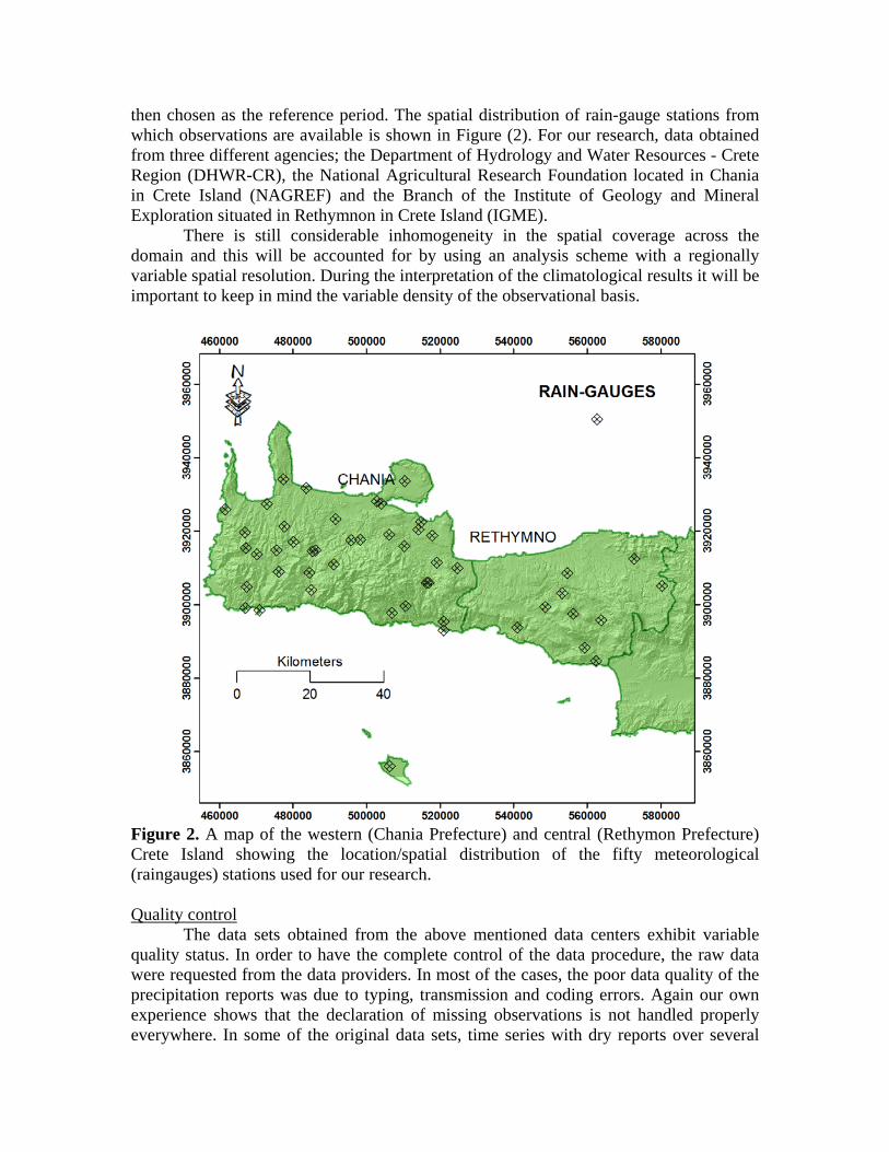
then chosen as the reference period. The spatial distribution of rain-gauge stations from which observations are available is shown in Figure (2). For our research, data obtained from three different agencies; the Department of Hydrology and Water Resources - Crete Region (DHWR-CR), the National Agricultural Research Foundation located in Chania in Crete Island (NAGREF) and the Branch of the Institute of Geology and Mineral Exploration situated in Rethymnon in Crete Island (IGME).

There is still considerable inhomogeneity in the spatial coverage across the domain and this will be accounted for by using an analysis scheme with a regionally variable spatial resolution. During the interpretation of the climatological results it will be important to keep in mind the variable density of the observational basis.

Figure 2. A map of the western (Chania Prefecture) and central (Rethymon Prefecture) Crete Island showing the location/spatial distribution of the fifty meteorological (raingauges) stations used for our research.

The data sets obtained from the above mentioned data centers exhibit variable quality status. In order to have the complete control of the data procedure, the raw data were requested from the data providers. In most of the cases, the poor data quality of the precipitation reports was due to typing, transmission and coding errors. Again our own experience shows that the declaration of missing observations is not handled properly everywhere. In some of the original data sets, time series with dry reports over several

Quality control

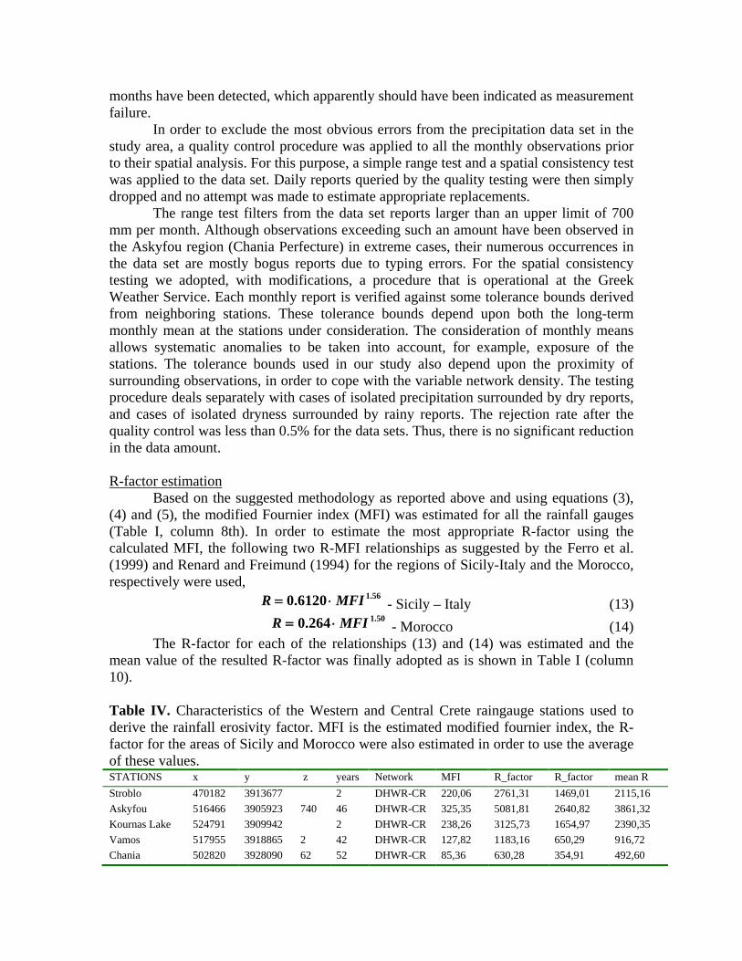
months have been detected, which apparently should have been indicated as measurement failure.

In order to exclude the most obvious errors from the precipitation data set in the study area, a quality control procedure was applied to all the monthly observations prior to their spatial analysis. For this purpose, a simple range test and a spatial consistency test was applied to the data set. Daily reports queried by the quality testing were then simply dropped and no attempt was made to estimate appropriate replacements.

The range test filters from the data set reports larger than an upper limit of 700 mm per month. Although observations exceeding such an amount have been observed in the Askyfou region (Chania Perfecture) in extreme cases, their numerous occurrences in the data set are mostly bogus reports due to typing errors. For the spatial consistency testing we adopted, with modifications, a procedure that is operational at the Greek Weather Service. Each monthly report is verified against some tolerance bounds derived from neighboring stations. These tolerance bounds depend upon both the long-term monthly mean at the stations under consideration. The consideration of monthly means allows systematic anomalies to be taken into account, for example, exposure of the stations. The tolerance bounds used in our study also depend upon the proximity of surrounding observations, in order to cope with the variable network density. The testing procedure deals separately with cases of isolated precipitation surrounded by dry reports, and cases of isolated dryness surrounded by rainy reports. The rejection rate after the quality control was less than 0.5% for the data sets. Thus, there is no significant reduction in the data amount.

Based on the suggested methodology as reported above and using equations (3), (4) and (5), the modified Fournier index (MFI) was estimated for all the rainfall gauges (Table I, column 8th). In order to estimate the most appropriate R-factor using the calculated MFI, the following two R-MFI relationships as suggested by the Ferro et al. (1999) and Renard and Freimund (1994) for the regions of Sicily-Italy and the Morocco, respectively were used,

R-factor estimation

56.16120.0 MFIR ⋅= - Sicily – Italy (13) 50.1264.0 MFIR ⋅= - Morocco (14)

The R-factor for each of the relationships (13) and (14) was estimated and the mean value of the resulted R-factor was finally adopted as is shown in Table I (column 10). Table IV. Characteristics of the Western and Central Crete raingauge stations used to derive the rainfall erosivity factor. MFI is the estimated modified fournier index, the R-factor for the areas of Sicily and Morocco were also estimated in order to use the average of these values. STATIONS x y z years Network MFI R_factor R_factor mean R Stroblo 470182 3913677 2 DHWR-CR 220,06 2761,31 1469,01 2115,16 Askyfou 516466 3905923 740 46 DHWR-CR 325,35 5081,81 2640,82 3861,32 Kournas Lake 524791 3909942 2 DHWR-CR 238,26 3125,73 1654,97 2390,35 Vamos 517955 3918865 2 42 DHWR-CR 127,82 1183,16 650,29 916,72 Chania 502820 3928090 62 52 DHWR-CR 85,36 630,28 354,91 492,60

Kalybes 514922 3922556 24 33 DHWR-CR 103,79 854,98 475,82 665,40 Mouri 510690 3899678 24 43 DHWR-CR 156,46 1621,89 880,68 1251,28 PaleaRoumata 480122 3917020 316 46 DHWR-CR 200,16 2381,79 1274,33 1828,06 Palaioxora 470982 3898560 48 26 DHWR-CR 90,98 696,11 390,49 543,30 Prasses 485374 3914558 520 16 DHWR-CR 285,28 4139,76 2168,30 3154,03 Souda 510372 3933641 152 42 DHWR-CR 88,63 668,36 375,50 521,93 Kandanos 476225 3909024 3 DHWR-CR 234,21 3043,24 1612,95 2328,09 Gadvos 506273 3856016 10 17 DHWR-CR 51,78 288,96 167,67 228,32 Meskla 495828 3917564 4 DHWR-CR 223,54 2829,73 1503,99 2166,86 Tavronitis 483600 3931738 15 35 NAGREF 98,56 788,75 440,33 614,54 ChaniaAgroki 504069 3927522 8 35 NAGREF 101,93 831,13 463,06 647,09 Drapanias 472991 3927382 29 19 NAGREF 109,32 927,06 514,34 720,70 Alikianos 491672 3923277 19 NAGREF 120,69 1081,77 596,62 839,20 Kandanos 476234 3908989 158 19 NAGREF 150,18 1521,53 828,22 1174,87 Koundoura 467146 3899182 59 9 NAGREF 72,49 488,44 277,75 383,10 Fragkokastello 520981 3892981 5 NAGREF 102,80 842,24 469,01 655,63 Falasarna 461635 3925886 12 NAGREF 94,88 743,26 415,89 579,58 Zymbragou 477730 3921328 235 19 NAGREF 155,51 1606,48 872,63 1239,56 Armenoi 514222 3920407 50 12 NAGREF 121,53 1093,62 602,90 848,26 Patsianos 521045 3895375 5 NAGREF 148,77 1499,21 816,53 1157,87 Anopolis 506878 3897748 600 12 IGME 135,78 1300,10 711,98 1006,04 Askyfou 516943 3905950 700 21 IGME 317,83 4899,77 2549,79 3724,78 Alikampos 519154 3911481 330 12 IGME 188,21 2163,75 1161,96 1662,85 Rodopou 477398 3934154 230 9 IGME 138,01 1333,60 729,61 1031,61 Epanoxori 484531 3908658 600 11 IGME 174,85 1928,90 1040,43 1484,66 Rogdia 467152 3915404 580 8 IGME 172,91 1895,65 1023,17 1459,41 Floria 475561 3914830 600 8 IGME 238,76 3136,05 1660,22 2398,14 Omalos 491146 3910915 1050 7 IGME 257,70 3532,60 1861,61 2697,10 Sirikari 466975 3919688 450 8 IGME 210,64 2579,21 1375,73 1977,47 Koystogerako 485010 3903952 530 12 IGME 164,36 1751,49 948,24 1349,87 Xasi(Boutas) 467500 3904906 370 14 IGME 122,97 1113,84 613,62 863,73 Prasses 486150 3914812 520 12 IGME 274,79 3904,66 2049,77 2977,21 Therissos 498286 3917629 580 21 IGME 194,51 2277,78 1220,78 1749,28 Melidoni 510334 3915922 400 21 IGME 198,40 2349,18 1257,55 1803,37 Kampoi 506136 3919063 560 12 IGME 211,71 2599,53 1386,16 1992,84 Spili 548679 3899338 390 34 DHWR-CR 176,99 1965,85 1059,58 1512,72 Melampes 559367 3888311 560 35 DHWR-CR 123,72 1124,50 619,26 871,88 Leykogeia 541121 3893756 90 32 DHWR-CR 127,08 1172,50 644,66 908,58 Kabousi 554689 3908615 580 29 DHWR-CR 129,05 1200,97 659,70 930,34 Gerakari 556273 3897534 580 31 DHWR-CR 204,36 2460,19 1314,64 1887,42 Garazo 572839 3912440 260 3 DHWR-CR 257,51 3528,50 1859,53 2694,02 Byzari 563871 3895736 310 29 DHWR-CR 118,26 1048,04 578,72 813,38 Boleones 553207 3903061 260 33 DHWR-CR 177,70 1978,17 1065,97 1522,07 Anogeia 580477 3905111 740 74 DHWR-CR 152,03 1550,82 843,54 1197,18 Agia Galini 562429 3884635 20 30 DHWR-CR 94,29 736,07 412,01 574,04

The calculated rainfall erosivity factors were interpolated with geostatistical as well as deterministic techniques. After applying and testing several geospatial prediction techniques the Ordinary Kriging (OK) interpolator was chosen for interpolating the point

Cross Validation

information (R-factor). Compared with the rest of interpolation methods, OK gave the best cross validation results and root mean squared (RMS) errors. RMS is given by the equation:

2

1

( )ni p io

i

DI DIRMS

n=

−=∑

(15)

where i pDI is the predicted value for site i, ioDI is the observed value for site i, and n the total number of sites.

“Kriging is a moderately quick interpolator that can be exact or smoothed depending on the measurement error model. “Instead of weighting nearby data points by some power of their inverted distance, ordinary kriging relies on the spatial correlation structure of the data to determine the weighting values. This is a more rigorous approach to modelling, as correlation between data points determines the estimated value at an unsampled point. Furthermore, ordinary kriging makes the assumption of normality among the data points” (Isaaks & Srivastava 1989).

Therefore, kriging methods work best if the data are approximately normally distributed. Transformations are used to make data normally distributed and satisfy the assumption of equal variability for the data. In the ArcGIS Geostatistical Analyst, the histogram (Figure 3) and normal QQPlots were used to check what transformations, if any, are needed to make the data more normally distributed. For a perfect normal distribution pattern skewness should be 0 and kurtosis equal to 3. For those parameters which did not show normal distribution, a Log transformation has to be applied to make the distribution closer to normal.

Figure 3. The statistical analysis of the rainfall erosivity data, as extracted from the ArcGIS Geostatistical Analyst package, is presented.

In this study, the semivariogram models (Circular, Spherical, Tetraspherical, Pentaspherical, Exponential, Gaussian, Rational Quadratic, Hole effect, K-Bessel, J-Bessel, Stable) were tested for the rainfall data set and the K-Bessel was selected.

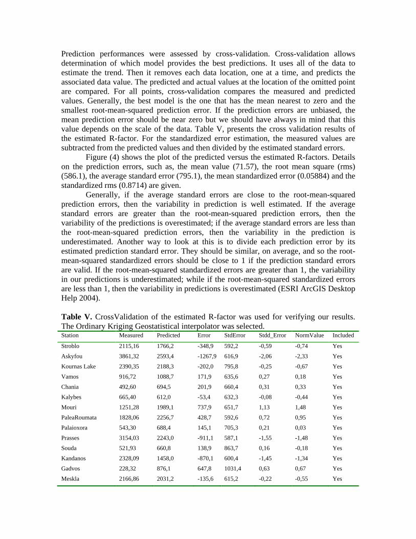
Prediction performances were assessed by cross-validation. Cross-validation allows determination of which model provides the best predictions. It uses all of the data to estimate the trend. Then it removes each data location, one at a time, and predicts the associated data value. The predicted and actual values at the location of the omitted point are compared. For all points, cross-validation compares the measured and predicted values. Generally, the best model is the one that has the mean nearest to zero and the smallest root-mean-squared prediction error. If the prediction errors are unbiased, the mean prediction error should be near zero but we should have always in mind that this value depends on the scale of the data. Table V, presents the cross validation results of the estimated R-factor. For the standardized error estimation, the measured values are subtracted from the predicted values and then divided by the estimated standard errors.

Figure (4) shows the plot of the predicted versus the estimated R-factors. Details on the prediction errors, such as, the mean value (71.57), the root mean square (rms) (586.1), the average standard error (795.1), the mean standardized error (0.05884) and the standardized rms (0.8714) are given.

Generally, if the average standard errors are close to the root-mean-squared prediction errors, then the variability in prediction is well estimated. If the average standard errors are greater than the root-mean-squared prediction errors, then the variability of the predictions is overestimated; if the average standard errors are less than the root-mean-squared prediction errors, then the variability in the prediction is underestimated. Another way to look at this is to divide each prediction error by its estimated prediction standard error. They should be similar, on average, and so the root-mean-squared standardized errors should be close to 1 if the prediction standard errors are valid. If the root-mean-squared standardized errors are greater than 1, the variability in our predictions is underestimated; while if the root-mean-squared standardized errors are less than 1, then the variability in predictions is overestimated (ESRI ArcGIS Desktop Help 2004). Table V. CrossValidation of the estimated R-factor was used for verifying our results. The Ordinary Kriging Geostatistical interpolator was selected. Station Measured Predicted Error StdError Stdd_Error NormValue Included

Stroblo 2115,16 1766,2 -348,9 592,2 -0,59 -0,74 Yes

Askyfou 3861,32 2593,4 -1267,9 616,9 -2,06 -2,33 Yes

Kournas Lake 2390,35 2188,3 -202,0 795,8 -0,25 -0,67 Yes

Vamos 916,72 1088,7 171,9 635,6 0,27 0,18 Yes

Chania 492,60 694,5 201,9 660,4 0,31 0,33 Yes

Kalybes 665,40 612,0 -53,4 632,3 -0,08 -0,44 Yes

Mouri 1251,28 1989,1 737,9 651,7 1,13 1,48 Yes

PaleaRoumata 1828,06 2256,7 428,7 592,6 0,72 0,95 Yes

Palaioxora 543,30 688,4 145,1 705,3 0,21 0,03 Yes

Prasses 3154,03 2243,0 -911,1 587,1 -1,55 -1,48 Yes

Souda 521,93 660,8 138,9 863,7 0,16 -0,18 Yes

Kandanos 2328,09 1458,0 -870,1 600,4 -1,45 -1,34 Yes

Gadvos 228,32 876,1 647,8 1031,4 0,63 0,67 Yes

Meskla 2166,86 2031,2 -135,6 615,2 -0,22 -0,55 Yes

Tavronitis 614,54 797,9 183,4 777,9 0,24 0,13 Yes

ChaniaAgrokip 647,09 658,7 11,6 635,9 0,02 -0,33 Yes

Drapanias 720,70 924,7 204,0 706,1 0,29 0,23 Yes

Alikianos 839,20 1597,9 758,7 715,1 1,06 1,34 Yes

Kandanos 1174,87 1859,9 685,1 602,2 1,14 1,64 Yes

Koundoura 383,10 599,2 216,1 684,9 0,32 0,39 Yes

Fragkokastello 655,63 942,9 287,3 702,0 0,41 0,55 Yes

Falasarna 579,58 1408,0 828,4 920,8 0,90 1,23 Yes

Zymbragou 1239,56 1725,3 485,7 633,6 0,77 1,04 Yes

Armenoi 848,26 973,0 124,7 595,4 0,21 0,08 Yes

Patsianos 1157,87 1376,3 218,4 674,9 0,32 0,44 Yes

Anopolis 1006,04 1135,6 129,6 767,0 0,17 -0,08 Yes

Askyfou 3724,78 2669,5 -1055,3 615,2 -1,72 -1,88 Yes

Alikampos 1662,85 2776,7 1113,9 609,3 1,83 2,33 Yes

Rodopou 1031,61 857,6 -174,0 770,9 -0,23 -0,61 Yes

Epanoxori 1484,66 2397,5 912,8 595,6 1,53 1,88 Yes

Rogdia 1459,41 1893,5 434,1 634,0 0,68 0,88 Yes

Floria 2398,14 2034,2 -364,0 580,6 -0,63 -0,81 Yes

Omalos 2697,10 2248,6 -448,5 664,5 -0,67 -0,88 Yes

Sirikari 1977,47 1207,6 -769,9 631,5 -1,22 -1,13 Yes

Koystogerako 1349,87 1568,7 218,8 755,0 0,29 0,28 Yes

Xasi(Boutas) 863,73 973,1 109,4 675,6 0,16 -0,13 Yes

Prasses 2977,21 2359,8 -617,4 590,4 -1,05 -1,04 Yes

Therissos 1749,28 2046,5 297,2 623,5 0,48 0,61 Yes

Melidoni 1803,37 1831,5 28,2 647,6 0,04 -0,28 Yes

Kampoi 1992,84 1225,3 -767,6 624,5 -1,23 -1,23 Yes

Spili 1512,72 1501,8 -10,9 698,4 -0,02 -0,39 Yes

Melampes 871,88 999,0 127,1 690,8 0,18 -0,03 Yes

Leykogeia 908,58 1267,8 359,2 946,6 0,38 0,50 Yes

Kabousi 930,34 1573,6 643,3 807,2 0,80 1,13 Yes

Gerakari 1887,42 1238,4 -649,0 667,5 -0,97 -0,95 Yes

Garazo 2694,02 1027,4 -1666,6 988,6 -1,69 -1,64 Yes

Byzari 813,38 1345,2 531,8 828,0 0,64 0,81 Yes

Boleones 1522,07 1417,6 -104,4 630,4 -0,17 -0,50 Yes

Anogeia 1197,18 1824,2 627,0 980,0 0,64 0,74 Yes

Agia Galini 574,04 693,4 119,4 774,1 0,15 -0,23 Yes

Figure 4. The calculated versus the predicted rainfall erosivity factor after the application of the cross-validation control on the spatial interpolation, is presented.

Soil erodibility (K-factor) was estimated with the help of the soil map provided by the Soil Geographical Data Base of Europe at a scale of 1:1,000,000 which is available online on:, (http://eusoils.jrc.it/). This map makes a distinction among coarse (<18% clay and >65% sand), medium (18–35% clay and >=15% sand, or 18% <clay and 15–65% sand), medium fine (<35% clay and <15% sand), fine (35– 60% clay) and very fine (clay >60%) soil texture types.

Soil erodibility factor (K)

After comparison between the geological maps of the Chania and Rethymnon Prefectures and the soil types available on the soil map we proceeded to the in situ check of soil samples for every geological formation which was included in each one of the four polygonal areas (i.e. soil types) of the Soil Geographical Data Base of Europe at Scale 1:1,000,000. Afterwards, the K-factor was calculated by means of the following formulae which were developed from global data of measured K values, obtained from 225 soil classes (Renard et al. 1997).

In the current work, the digital elevation model (DEM) of the study area with a cell size of 20 m was used for the calculation of the LS factor. There are many formulas capable of calculating the L and S factors. In the new array-based framework that has been adopted, the overall flow path-based iterative slope-length accumulation and LS factor computation steps were performed using the RUSLE Version 4 (an AML) (Van Remortel et al. 2001). As a result, each 20 m cell of the grid surface of each one of the watersheds was assigned an LS value.

Slope-length (L) and slope steepness (S) factors

Cover Management factor (C)

A scene of Landsat ETM images acquired on 30 June 2000 with a spatial resolution of 30 m was used. These images consisted of band 1: 0.45–0.53 mm, band 2: 0.52–0.60 mm, band 3: 0.63–0.69 mm, band 4: 0.76–0.90 mm, band 5: 1.55–1.75 mm, and band 7: 2.08–2.35 mm. The snow area of the image was masked and the NDVI image was then produced. After the production of the NDVI image, the following formula was used to generate a C-factor surface from NDVI values (Van der Knijff et al. 1999; 2000, Van Leeuwen and Sammons 2004):

C=e (-α ((NDVI)/ (β-NDVI))) (16) where α and β are unitless parameters that determine the shape of the curve relating NDVI and the C-factor. Van der Knijff et al. (1999, 2000) found that this scaling approach gave better results than assuming a linear relationship. Finally, the values of 2 and 1 was selected for the parameters α and b respectively, since the resulted values were in a good agreement with the values mentioned in the related literature and had the best correlation with the Corine Land Cover map 2000 (CLC2000 100m, version 1) of the European Environment Agency (©EEA, Copenhagen, 2000; http://www.eea.europa.eu). This map has a resolution of 100 m and uses 18 land use categories for the study area from a total of 44 land uses of level 3. As the C factor ranges between 0 and 1, a value of 0 was assigned to a few pixels with negative values and a value of 1 to pixels with value greater than 1. Results and Discussion

By using the values of the R factor estimated for each investigated raingauge (50 meteo-stations in western and central Crete) and a kriging interpolation method, the isoerosivity map of the study area is produced as is shown in Figure 5. The average annual R factor value varies from 869 to 3686 MJ mm ha−1 h−1 year−1 (Table VI). There is more rainfall erosivity in the south (where White Mountains are located) and in the northeastern part of the study area that coincides with higher elevation. In other words, decreasing R factor has a strong relationship with the decreasing trend of elevation. The final R-factor map for the study area is presented in Figure 5.

Rainfall erosivity factor

The calculated R factors are showing high erosivity (3020-3687 MJ mm ha-1 year-

1) in the broader area of White Mountains. Medium to high erosivity (2500-3687 MJ mm ha-1 year-1) is observed in the southern part of Kalami and Vrysses watersheds and that fact is in a good agreement with the results of Kouli et al. (2007). High values of rainfall erosivity are also shown in the northeastern part of the Geropotamos watershed where the Talea Mountains are lying. As the topography changes going from steep (mountainous areas) to flat relief (coastal areas) the erosivity decreases normally from 2500 to 868 MJ mm ha-1 year-1 in the northern part of Kalami watershed. Moreover, some statistical information for the investigated watersheds are given in Table VI concerning the number of pixels and the minimum, maximum and average R-factor value for each one of the nine watersheds of the central Crete Island. Table VI. Statistical data of the R-factor for each watershed in the study area

NAMES Num. of Pixels MIN R-fac MAX R-fac RANGE MEAN STD

Kalami 1921 868,81 1892,62 1023,81 1553,95 278,9340

Vrysses 2811 1182,27 3686,43 2504,16 2072,66 411,0890

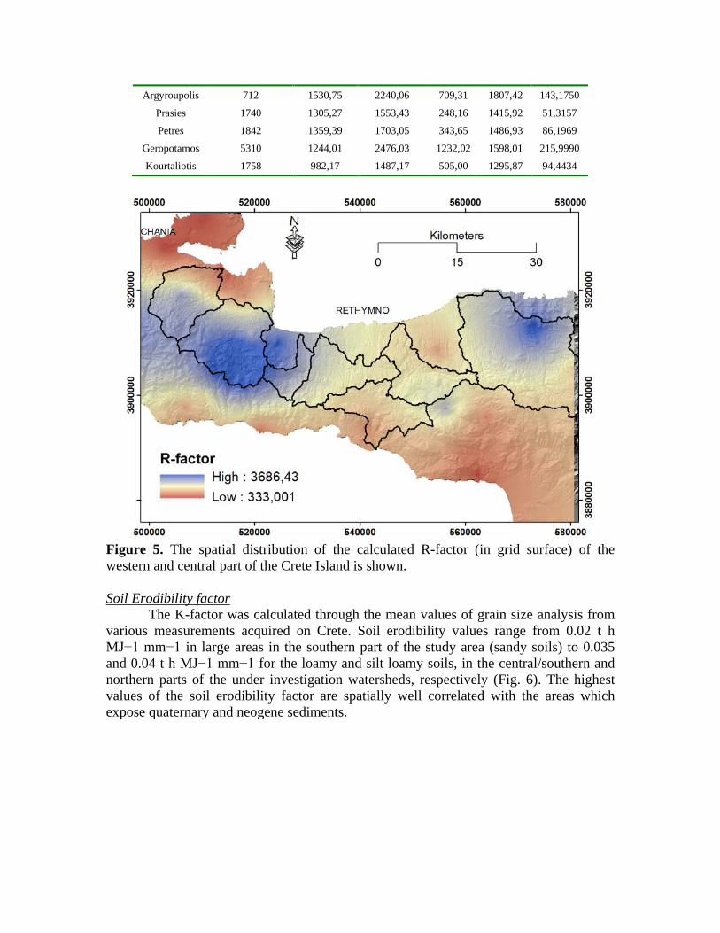
Argyroupolis 712 1530,75 2240,06 709,31 1807,42 143,1750

Prasies 1740 1305,27 1553,43 248,16 1415,92 51,3157

Petres 1842 1359,39 1703,05 343,65 1486,93 86,1969

Geropotamos 5310 1244,01 2476,03 1232,02 1598,01 215,9990

Kourtaliotis 1758 982,17 1487,17 505,00 1295,87 94,4434

Figure 5. The spatial distribution of the calculated R-factor (in grid surface) of the western and central part of the Crete Island is shown.

The K-factor was calculated through the mean values of grain size analysis from various measurements acquired on Crete. Soil erodibility values range from 0.02 t h MJ−1 mm−1 in large areas in the southern part of the study area (sandy soils) to 0.035 and 0.04 t h MJ−1 mm−1 for the loamy and silt loamy soils, in the central/southern and northern parts of the under investigation watersheds, respectively (Fig. 6). The highest values of the soil erodibility factor are spatially well correlated with the areas which expose quaternary and neogene sediments.

Soil Erodibility factor

Figure 6. The Soil Erodibility Factor (K) map of the study area and the polygonal vector layer representing the seven selected watersheds are depicted.

The LS factor was calculated using the DEM of the watersheds as well as considering the interactions between topography and flow accumulation. In the new array-based framework that has been adopted, the overall flow path-based iterative slope-length accumulation and LS factor computation steps were performed using the RUSLE Version 4 (Van Remortel et al. 2001). Version 4 is intended to correct an order-of-operations error in earlier versions that affected the computation of the slope steepness constituent, generally yielding higher (by about 5-10%) LS factor values. This is the latest version of the RUSLE code that was modified from the original USLE-based code by Rick D. Van Remortel and Mathew E. Hamilton of the Remote Sensing and Technical Services Department, Lockheed Martin Environmental Services. Calculates LS Factor using DEM data according to RUSLE-based criteria. (Van Remortel et al. 2001).

LS factor

The file will execute independently at the command-line prompt, either with an argument string or with a series of interactive prompt responses, to perform an LS run for a single spatial reporting unit (e.g., one watershed at a time). Users also have a third option of running the lsfac.aml AML shell program in ArcInfo Workstation which automatically calls upon the executable as necessary to perform the LS factor processing for single or multiple spatial reporting units (e.g., a large number of study area watersheds in a single run).

It can be seen that the LS factor varies from 0 to 148. However, some specific areas with steep slopes (such as along the rivers) have greater LS values. Figure 7 shows the LS-factor grid maps of the study watersheds.

The Vrysses watershed shows the greatest LS factor among the seven studied watersheds (Table VII). The topographic factor ranges from 0 in the flat zones to 148 at the steep slopes in the southern part of the basin. Although Kalami basin is characterized by the greatest elevation drop of 2187 m and consequently the greatest LS factor, the great values are present in a limited part of the basin (Fig. 6). On the other hand, Argyroupolis watershed shows maximum LS factor equal to 118 but its mean value is significantly greater than this of Vrysses basin (Fig. 6). This fact implies extended areas of steep slopes which are prone to severe erosion. In the opposite hand, Petres watershed is characterized by relatively small LS factor values and this is consistent with its relatively low elevation values and the smallest extent of the watershed (Figure 7). It is noteworthy, the fact that despite its relatively low maximum LS value (i.e. 93), Prasies basin shows high mean LS factor values of 110 and 7.88 in comparison with the Geropotamos and especially Kourtaliotis watersheds. Table VII. Statistical data of the LS-factor for each watershed in the study area

Watersheds Min Max Mean Std Kalami 0 117 7.65 8.69 Vrysses 0 148 8.52 9.37 Argyroupolis 0 118 9.36 9.28 Prasies 0 93 7.88 8.05 Petres 0 99 5.62 6.78 Geropotamos 0 111 6.68 7.72 Kourtaliotis 0 121 6.80 7.75

Figure 7. The LS maps as calculated from the processing of DEM of the seven selected watersheds.

The C factor map was prepared based on NDVI (Figure 8) applying the NDVI-C relationship proposed by Van der Knijff et al. (1999, 2000). In general, this factor has completely inverse relationship with NDVI. As seen from the Figure 9, the greatest amount of this parameter coincides with the urban areas along the coastline in the northern part of the island (magenta color) whereas the least amount is related to the area with dense forest vegetation (deep green color).

Cover Management factor

The NDVI thematic map resulted from the Landsat-ETM satellite image of the study area showing a range from -0.32 to 0.85 (Figure 8). The Corine Land Cover vector map was overlain to the pixel by pixel estimated cover management factor grid (Fig. 8) and the mean C value for every Corine class was calculated (Table VI). As a result, the mean C values range inside the watersheds from 0.13 for the forest class to 0.785 for the bare rocks class (Table VIII). The C-values for forest are near 0 and for the bare rocks tending to 1 which looks realistic. The predicted C-values of the arable classes depend on crop type and management practices.

The approach followed here it was based to the available data. To improve the results, satellite images with better geometric and spectral characteristics can provide detailed information, as well as field measurements can be proved efficient in order to relate biophysical properties (like the C-factor) to remotely-sensed data. Table VIII The average C factor values for the several land uses of the study area (Kouli et al. 2009).

Land Use Mean Broad-leaved forest 0.130266 Fruit trees and berry plantations 0.178411 Mixed forest 0.182351 Vineyards 0.294141 Olive groves 0.304188 Land principally occupied by agriculture 0.307676 Coniferous forest 0.338087 Transitional woodland-shrub 0.375549 Sclerophyllous vegetation 0.412805 Complex cultivation patterns 0.428191 Non-irrigated arable land 0.496456 Moors and heathland 0.500111 Pastures 0.543197 Natural grasslands 0.545464 Construction sites 0.548493 Beaches, dunes, sands 0.575484 Sparsely vegetated areas 0.644916 Bare rocks 0.785093

Figure 8. The NDVI thematic map resulted from the Landsat-ETM satellite image of the study area showing a range from -0.32 to 0.85.

Figure 9. The cover management factor distribution which derived from the NDVI image (Figure 8).

Soil loss values were computed by overlaying the four grid surfaces of each one of the seven catchments: the grid surface representing the R-factor values, the grid surface representing the K-factor values, the grid surface representing the C-factor values and the grid surface representing the LS-factor values in the ArcView GIS software environment.

Soil Loss and hydro-geo-tectonic parameters

Soil loss values (Table IX) range between 0 and 5134 t/ha yr for the Kalami watershed, with a mean value of 204.42 t/ha yr, between 0 and 5760 t/ha yr with a mean value of 335.66 t/ha yr for the Vrysses watershed, between 0 and 4545.96 t/ha yr for Argyroupolis basin with a mean value of 269.49 t/ha yr, between 0 and 1920.58 t/ha yr for the Prasies basin (mean value equal to 108.58 t/ha yr), between 0 and 3149.26 t/ha yr for the Petres watershed (mean value equal to 85.52 t/ha yr), between 0 and 4932.78 t/ha yr for the Geropotamos basin with a mean value of 170.06 t/ha yr, between 0 and 4254 t/ha yr for the Keritis watershed (mean value equal to 193.527 t/ha yr) and between 0 to 2792.19 t/ha yr for the Kourtaliotis watershed with a mean value of 94.73 t/ha yr. The highest mean soil loss values are spatially correlated with the steepest slopes.

The resulting map for the study area can be seen in Figure 11. Soil loss values range between 0 and 5761 (t/ha-1 year-1). With regard to the spatial variation, the southwest and northeastern part of the whole study area is more prone to erosion than the southeastern, northwestern and central area. However, it should be noted that areas with amount of erosion greater than 75 ton h-1 year-1 have been distributed in the watershed non-uniformly (Figure 11). Reason for this high soil loss is related to its close relationship with high elevation and steep topography (LS factor) and high rainfall erosivity (see figure 5). Table IX. Statistical data of the estimated annual soil loss for each watershed in the study area

Watersheds Min Max Mean Std Kalami 0 5134.06 204.42 322.40 Vrysses 0 5760.67 335.66 428.82 Argyroupolis 0 4545.96 269.49 361.78 Prasies 0 1920.58 108.58 142.79 Petres 0 3149.26 85.52 132.10 Geropotamos 0 4932.78 170.06 257.96 Kourtaliotis 0 2792.19 94.73 140.20

Figure 10. Soil loss maps for each studied watershed (from west to east), after the application of the RUSLE equation are presented.

Figure 11. The soil loss map in tons/ha yr for the watersheds under investigation, after the application of the RUSLE equation, is presented.

Correlations between the tectonic characteristics which govern the geomorphic evolution of the watersheds and the calculated annual soil losses can be easily defined. Generally, the tectonic characteristics (faults and other lineaments) which are usually responsible for sedimentation and erosion processes (changes in relief and steepness) are in direct correlation with the soil losses. Figures (12a and 12b) are in an agreement with the aforementioned assumption since high soil losses are observed in the north-eastern part of Kalami and Vrysses watersheds northern the fault system directed NW-SE and into the central part (tectonic graben oriented WNW-ESE) of the Geropotamos basin, respectively.

Figure 12. The correlation between the tectonic features and the estimated annual soil loss is presented for Kalami and Vrysses watersheds (upper figure) and for Geropotamos basin (lower figure).

From the hydrolithological point of view, the geological formations composed the watersheds under investigation are classified into six hydro-lithological units (Soupios et al. 2009): a) (K1, K2) high to medium permeability rocks, which comprise the karstic limestones of Tripolis and Trypalion nappes and dolomitic rocks, b) (P1) fluctuant permeability formations which composed of recent to present alluvial deposits, eluvial mantle materials, fluvial deposits, talus cones, dunes and conglomerates in places, c) (P2) medium to low permeability formations which consists mainly of Miocene and Pliocene deposits (Neogene marly limestones and conglomerates), d) (P3) low to very low permeability formations which composed of Pliocene and Miocene marls and other impermeable Neogene formations and e) (I2) low to very low permeability formations which mainly composed of metamorphic (phyllites, etc) and rocks of all the geological units and nappes (including the Ionion nappe).

Based on the aforementioned and annotated the Table X, we can conclude that areas composed of high permeability rocks (K1 and K2) such as karstic and dolomitic limestones, present the highest soil losses (Figure 13) since the water passed through the fracture chaotic system, accelerate the erosion processes producing large quantities of terra rossa and other alluvial sediments. Consequently, a correlation between the hydrolithological characteristics of the geological formations of the studied watersheds and the soil losses is observed. Table X. The hydrolithological characteristics (permeability) in comparison with the calculated soil losses for the Kalami watershed is presented.

PERMEABILITY AREA RANGE MEAN STD SUM

I2 17240800 1356,56 127,324 141,369 2702570

K1 65792200 5134,06 274,760 374,873 22255600

K2 6249450 3490,90 504,032 445,590 3878020

P1 9313260 1068,43 28,067 70,736 321819

P2 17781800 1690,87 69,864 99,984 1529460

P3 7780540 1081,61 58,610 104,573 561429

Figure 13. The mean annual soil loss predicted values for each one of the six different hydrolithological units which are present in Kalami and Vrysses watersheds.

The variation in soil nutrients is crucial to the understanding of productivity of soil undergoing erosion overall, as the latter can result in a decline in soil quality and crop production in the whole landscape (Ni and Zhang 2007). Tillage erosion, the dominant soil redistribution process on terraced fields, was found to be a major contributor to the variation in soil chemical properties in the terraced field landscape, while water erosion plays an important role in the variation in soil chemical properties in the long slope landscape. Therefore, the correlation between the chemical concentration and soil loss models can be a possible method of characterizing the process of transportation of sediment and chemicals in watersheds.

Soil Loss and chemical parameters

The methodology used for modeling the possible correlation between the chemical parameters of the phreatic groundwater of Geropotamos Basin and the calculated soil loss utilizes standard ArcMap commands and functions and is divided into the following steps:

• The hydrological modeling of the Geropotamos basin based on the rainfall data was executed.

• The soil loss as a result of water erosion is calculated applying the RUSLE model, • The raster representation of the concentration of six chemical parameters (i.e.,

Conductivity, Hardness, Na, NO3, pH and SO4) using the Ordinary Kriging Interpolator,

• Application of statistical techniques to examine possible spatial dependence between the chemical concentrations with the estimated annual soil losses for the area of Geropotamos basin (Table XI).

Table (XI) shows the cross correlation between the chemical model (six chemical parameters - conductivity, hardness, Na, NO3, SO4, pH) and the soil loss model in Geropotamos watershed. The correlation coefficient between the two models is found to be between 0.0006 and 0.2, which reflects a weak negative correlation between the two models. Table XI. The correlation matrix between annual soil loss and six selected groundwater chemical parameters Layer Soil_loss Conductivity Hardness Na NO3 pH SO4

Soil_loss 1 -0,00066 0,02109 -0,01743 0,09734 -0,27068 -0,04351

Conductivity -0,00066 1 0,94974 0,9584 0,42258 -0,11378 0,43214

Hardness 0,02109 0,94974 1 0,916 0,48332 -0,03341 0,33171

Na -0,01743 0,9584 0,916 1 0,41372 -0,09243 0,44147

NO3 0,09734 0,42258 0,48332 0,41372 1 0,05813 0,1003

pH -0,27068 -0,11378 -0,03341 -0,09243 0,05813 1 -0,1386

SO4 -0,04351 0,43214 0,33171 0,44147 0,1003 -0,1386 1

Modeling soil loss using Ordinary Least Squares linear regression approach

In order to model annual soil loss according to its relationship with selected geomorphic and remotely sensed derived parameters we performed the global Ordinary Least Squares linear regression. For this purpose, a fishnet of 128 points was created covering the under investigation watershed areas (figure 14). The horizontal distance between adjacent points was 4400m while the vertical distance was equal to 2200 meters. For each one of the 128 points, parameters such as annual soil loss, elevation, slope angle, NDVI and mean annual precipitation were obtain using the raster thematic layers inside the GIS environment.

The correlation and regression coefficients between the calculated annual soil loss values (depended parameter) and selected independed parameters related to topography (elevation and slope angle), extracted from satellite data (NDVI) and derived from meteorological data (corrected mean annual rainfalls) were then calculated. At a first level we used separately each one of the explanatory parameters and all of them together in a next level. Both the Multiple R-Squared and Adjusted R-Squared values which are measures of model performance are given in Table XII. The values can possibly range from 0.0 to 1.0. The Adjusted R-Squared value is always found to be lower than the Multiple R-Squared value as it shows model complexity (the number of variables). For that reason is a more accurate measure of model performance. Adding an additional explanatory variable to the model usually increases the Multiple R-Squared value, and decreases the Adjusted R-Squared value.

In an effort to create a regression model of soil loss (the value of annual soil loss associated with each sample point is the dependent variable) the Adjusted R-Squared value was found to be equal to 0.58 and probably indicates that the model (the selected explanatory variables) explains approximately the 58% of the variation in the dependent

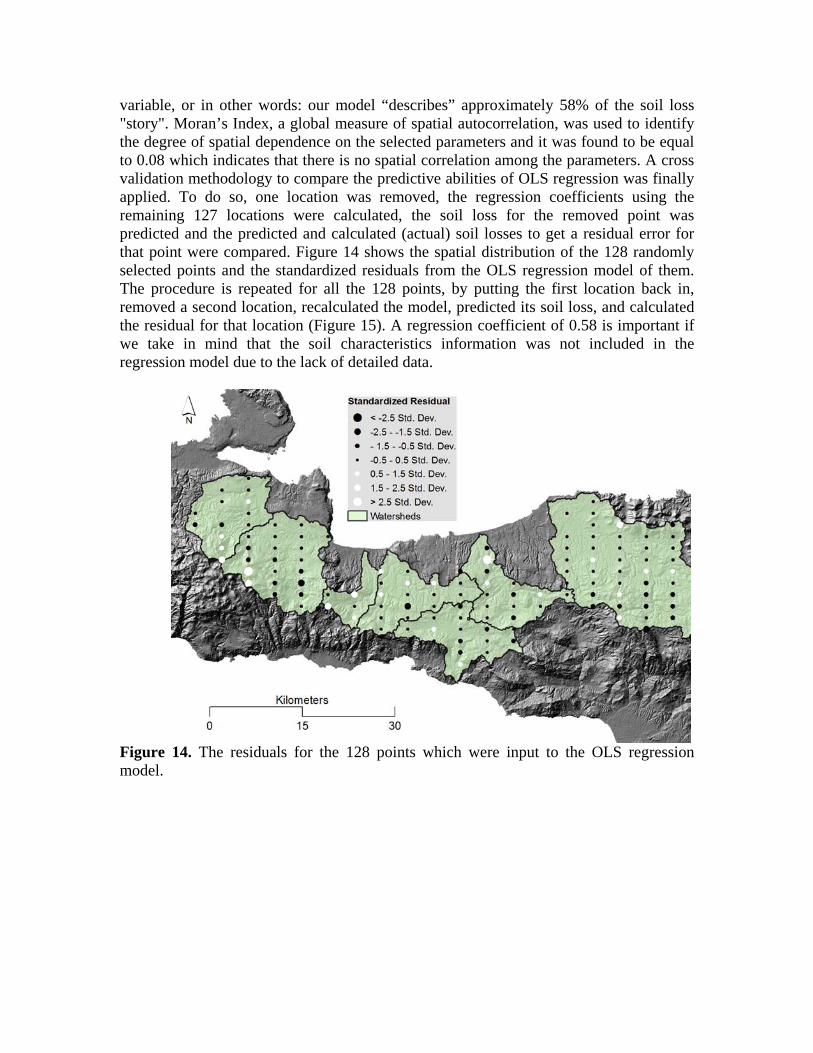
variable, or in other words: our model “describes” approximately 58% of the soil loss "story". Moran’s Index, a global measure of spatial autocorrelation, was used to identify the degree of spatial dependence on the selected parameters and it was found to be equal to 0.08 which indicates that there is no spatial correlation among the parameters. A cross validation methodology to compare the predictive abilities of OLS regression was finally applied. To do so, one location was removed, the regression coefficients using the remaining 127 locations were calculated, the soil loss for the removed point was predicted and the predicted and calculated (actual) soil losses to get a residual error for that point were compared. Figure 14 shows the spatial distribution of the 128 randomly selected points and the standardized residuals from the OLS regression model of them. The procedure is repeated for all the 128 points, by putting the first location back in, removed a second location, recalculated the model, predicted its soil loss, and calculated the residual for that location (Figure 15). A regression coefficient of 0.58 is important if we take in mind that the soil characteristics information was not included in the regression model due to the lack of detailed data.

Figure 14. The residuals for the 128 points which were input to the OLS regression model.

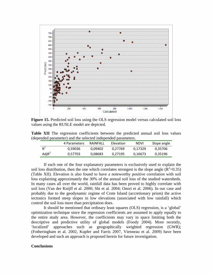
Figure 15. Predicted soil loss using the OLS regression model versus calculated soil loss values using the RUSLE model are depicted. Table XII The regression coefficients between the predicted annual soil loss values (depended parameter) and the selected independed parameters.

4 Parameters RAINFALL Elevation NDVI Slope angle R2 0,59036 0,09402 0,27769 0,17329 0,35706 AdjR2 0,57703 0,08683 0,27195 0,16673 0,35196

If each one of the four explanatory parameters is exclusively used to explain the

soil loss distribution, then the one which correlates strongest is the slope angle (R2=0.35) (Table XII). Elevation is also found to have a noteworthy positive correlation with soil loss explaining approximately the 30% of the annual soil loss of the studied watersheds. In many cases all over the world, rainfall data has been proved to highly correlate with soil loss (Van der Knijff et al. 2000; Shi et al. 2004; Onori et al. 2006). In our case and probably due to the geodynamic regime of Crete Island (accretionary prism) the active tectonics formed steep slopes in low elevations (associated with low rainfall) which control the soil loss more than precipitation does.

It should be mentioned that ordinary least squares (OLS) regression, is a ‘global’ optimization technique since the regression coefficients are assumed to apply equally to the entire study area. However, the coefficients may vary in space limiting both the descriptive and predictive utility of global models (Foody 2004). More recently, ‘localized’ approaches such as geographically weighted regression (GWR); (Fotheringham et al. 2002, Kupfer and Farris 2007, Vienneau et al. 2009) have been developed and such an approach is proposed herein for future investigation. Conclusions

The RUSLE model was applied in order to estimate soil loss in seven major watersheds of the western and central part of Crete Island. Detailed data for the computation of the R-, K- and C- factor were not available; therefore these parameters were estimated either by means of general or approximation formulae or by processing available satellite images (i.e. for the extraction of the cover management-C- factor ). Moreover, the estimation of LS- factor was performed with the use of a GIS automated technique to generate slope length and slope steepness.

The results of the application of the RUSLE model seems to be consistent with those obtained for other Mediterranean watersheds of similar characteristics. Moreover, it confirmed that the estimated soil loss occurring in the studied watersheds is well correlated with geomorphic, tectonic and hydrolithological characteristics. Among them slope angle seems to explain better the erosion processes.

However, we must note the complete lack of data for the estimation of P-factor, which was set to 1. The current study shows that even if some uncertainties are present, the RUSLE model can be efficiently applied at the basin scale with quite modest data requirements in a typical Mediterranean environment such as the investigated river basins. Further analysis of the P-factor could improve the results. However, the obtained results are still very important as they quantify the soil loss and point the water basins which are exposed to great danger of soil erosion, a serious problem in the island of Crete, the biggest Greek island with great agricultural activity. Acknowledgments We are grateful to Prof. F. Sdao and to other two anonymous reviewers for their critical comments that led to substantial changes of the original manuscript. We would like to thank the Crete Region, the NAGREF and the IGME (Branch of Crete) institutions for providing the raw (uncorrected) rainfall data. We should also express our appreciation to Dr. N. Lydakis-Simantiris for helping DK to complete and interpret the chemical analyses from the Geropotamos watershed.

References Abu Hammad A., Lundekvam H., Børresen T. (2005) Adaptation of RUSLE in the

eastern part of the Mediterranean region. Environmental Management, 34, 6, pp.829–841.

ArcGIS Desktop Help. (2004) ArcGIS Desktop Help included in ArcMap Version 9.1 software by ESRI.

Arhonditsis G., Giourga C., Loumou A. and Koulouri M. (2002) Quantitative assessment of agricultural runoff and soil erosion using mathematical modeling: Applications in the Mediterranean region. Environmental Management 30:434–453.

Arnoldus, H. M. J. (1980) An approximation of the rainfall factor in the Universal Soil Loss Equation. In: Assessment of Erosion (ed. by M. De Boodt & D. Gabriels), 127-132. Wiley, Chichester, UK.

Aronica G. and Ferro V. (1997) Rainfall erosivity over Calabrian region. Hydrol. Sci. J. 42(1), 35-48.Bergsma, E. (1980) Provisional rain-erosivity map of The Netherlands. In: Assessment of Erosion (ed. by M. De Boodt & D. Gabriels). Wiley, Chichester, UK.

Ascough J.C., Baffaut C., Nearing M.A., Liu B.Y. (1997) The WEPP watershed model: I. Hydrology and Erosion, Trans. Am. Soc. Agric. Eng.,40(4), pp.921-933.

Bagarello V. (1994) Procedure semplificate per la stima del fattore climatico délia USLE nelPambiente molisano (Simplified procedures for estimating the climatic factor of the USLE in Molise, in Italian). Atti delta Giornata di Studio Sviluppi Recenti delle Ricerche sull'Ewsione e sul suo Controllo (Bari, 17-18 February 1994).

Banasik K. and Gôrski D. (1994) Rainfall erosivity for South-East Poland. In: Conserving Soil Resources. European Perspectives (ed. by R. J. Rickson), pp.201-207. Lectures in Soil Erosion Control, Silsoe College, Cranfield University, UK.

Benkobi L., Trlica M. J. and Smith J. L. (1994) Evaluation of a refined surface cover subfactor for use in RUSLE. Journal of Range Management, 47, pp.74–78.

Bergsma E. (1980) Provisional rain-erosivity map of The Netherlands. In: Assessment of Erosion (ed. by M. De Boodt and D. Gabriels). Wiley, Chichester, UK.

Biesemans J., Meirvenne M. V. and Gabriels D. (2000) Extending the RUSLE with the Monte Carlo error propagation technique to predict long-term average oV-site sediment accumulation. Journal of Soil and Water Conservation, 55, pp.35-42.

Blanpied N.(1984) Farm Policy: The Politics of Soil, Surpluses, and Subsidies (Washington, DC: Congressional Quarterly, Inc., 1984.)

Bolinne A., Laurant A. and Rosseau P. (1980) Provisional rain-erosivity map of Belgium. In: Assessment of Erosion (ed. by M. De Boodt & D. Gabriels), pp.111-120. Wiley, Chichester, UK.

Boyle M. (2002) Erosion’s contribution to greenhouse gases. Erosion Control. 9, pp.64–67.

Brown L.R. (1984) Conserving soils. In: Brown, L.R. (Ed.), State of the World. Norton, New York, pp.53– 75.

Castrignanò A., Buttafuoco G., Canu A., Zucca C., and Madrau S. (2008) Modelling Spatial Uncertainty of Soil Erodibility Factor using Joint Stochastic Simulation, Land Degrad. Develop. 19, pp.198-213

Chartzoulakis K.S. (2001) Paranychianakis, N.V., Angelakis, A.N., Water resources management in the island of Crete, Greece, with emphasis on the agricultural use, WaterPolicy, Vol.3, pp.193-205.

Chowdary V.M., Rao N.H. and Sarma P.B.S. (2003) GIS-based decision support system for groundwater assessment in large irrigation project areas. Agric. Water Manage. 62, pp.229–252.

Cox C., Madramootoo C. (1998) Application of Geographic Information Systems in watershed management planning in St. Lucia. Computers and Electronics in Agriculture 20, pp.229–250.

Erdas Field Guide (2005|) Geospatial Imaging, LLC, Norcross Georgia. Erdogan E.H., Erpul. G., Bayramin I. (2007) Use of USLE/GIS Methodology for

Predicting Soil Loss in a Semiarid Agricultural Environment. Environ Monit Assess 131 pp.153–161.

Favis-Mortlock D.(2007) (last Updated Tue Feb 12 2008). “Soil erosion site”. Retrieved January 2010 from http://www.soilerosion.net/

Fernandez C., Wu J.Q., McCool D.K., Stockle C.O. (2003) Estimating water erosion and sediment yield with GIS, RUSLE,and SEDD. J. Soil Water Conserv. 58, pp.128–136.

Ferro V., Giordano G. and Lovino M. (1991) Isoerosivity and erosion risk map for Sicily. Hydrol. Sci. J. 36(6), pp.549-564.

Ferro V., Porto P. and Yu B. (1999) A comparative study of rainfall erosivity estimation for Southern Italy and southeastern Australia, Hydrological Sciences—Journal—des Sciences Hydrologiques, 44(1).

Foody G.M. (2004) Spatial nonstationarity and scale dependency in the relationship between species richness and environmental determinants for the sub- Saharan endemic avifauna. Global Ecol Biogeogr 13, pp.315–320.

Foster, G. R., D. C. Yoder, G. A. Weesies, D. K. McCool, K. C. McGregor, and R. L. Bingner (2002) User’s guide—Revised Universal Soil Loss Equation Version 2 (RUSLE 2). USDA–Agricultural Research Service, Washington, DC.

Foster G. (2005) Revised Universal Soil Loss Equation Version 2 (RUSLE 2), Science Documentation, USDA-Agricultural Research Service, Washington D.C.

Fotheringham A.S, Brunsdon C., Charlton M. (2002) Geographically weighted regression: the analysis of spatially varying relationships. Wiley, Chichester

Fu G., Chen S., McCool K.D. (2006) Modelling the impacts of no-till practice on soil erosion and sediment yield using RUSLE, SEDD and ArcView GIS. Soil and Tillage Research, 85, pp.38-49.

Gabriels D., Cadron W. and De Mey P. (1986) Provisional rain erosivity maps of some EC countries. Proc. Workshop on Erosion Assessment and Modelling (Brussels, Belgium).

Gong J. (2001) Geography Information System. Science Publishing Company, Beijing. Govers G, Lobb DA, Quine TA (1999) Tillage erosion and translocation: emergence of a

new paradigm in soil erosion research. Soil and Tillage Research 51, 167-174. Grimm M., Jones R. and Montanarella L. (2002) Soil Erosion Risk in Europe, European

Soil Bureau Institute for Environment & Sustainability JRC Ispra. Haan C.T., Barfield B.J., Hayes J.C. (1994) Design Hydrology and Sedimentology for

Small Catchments. Academic Press, San Diego, CA, USA 588pp.

Hussein M. H. (1986) Rainfall erosivity in Iraq. J. Soil Wat. Conserv., pp.336-338. Isaaks E.H. and Srivastava, M. (1989) An Introduction to Applied Statistics. New York:

Oxford University Press. Keller E.A. (1996) Environmental geology. Prentice-Hall, New Jersey Knisel W.G. and Turtola E. (2000) Gleams model application on a heavy clay soil in

Finland, Agricultural Water Management, 43(3), pp. 285-309 Kouli M., Lydakis-Simantiris N. & Soupios P. (2008) GIS-based aquifer modeling and

planning using integrated geoenvironmental and chemical approaches, Groundwater: Modeling, Management and Contanimation (eds. Luka F. König and Jonas L. Weiss), USA: Nova Publishers.

Kouli M., Soupios P. and Vallianatos F. (2009) Soil erosion estimation using the Revised Universal Soil Loss Equation (RUSLE) in a GIS framework, Chania, Northwestern Crete, Greece, Environ. Geol., doi 10.1007/s00254-008-1318-9.

Krahl J., Kauffmann G., Kozur H., Richter D., Forster O., Heinritzi F. (1983) Neue Daten zur Biostratigraphie und zur tektonischen Lagerung der Phyllit-Gruppe und der Trypali-Gruppe aufder Insel Kreta (Griechenland). Geol Rundsch 72, pp.1147–1166

Kupfer J.A., Farris C.A. (2007) Incorporating spatial non-stationarity of regression coefficients into predictive vegetation models Landscape Ecol 22, pp.837-852.

Lal R. (1990) Soil Erosion in the Tropics: Principles and Management. McGraw-Hill, New York.

Lal R. (1994) Soil erosion by wind and water: problems and prospects. In: Lal, R. (Ed.), Soil Erosion Research Methods. 2nd ed. Soil andWater Conservation Society, St. Lucie Press, pp.1–9.

Lal R. (2001) Soil conservation for C sequestration. In: Stott, D.E., Mohtar, R.H., Steinhardt, G.C. (Eds.), Proceedings of the 10th International Soil Conservation Organization Meeting, May 24–29. pp.459–465.

Leonard R.A., Knisel W.G. and Still D.A. (1987) GLEAMS: Groundwater loading effects of agricultural management systems. Trans. Am. Soc. Agric. Eng. 30(5) pp.1403–1418.

Lewis L.A., Verstraeten G., Zhu H. (2005) RUSLE applied in a GIS framework: calculating the LS factor and deriving homogeneous patches for estimating soil loss. International Journal of Geographical Information Science 19 (7), pp.809–829.

Li C., Li J.X., Zhu F.-G., Lu. C., Chen Z., Wu T., Wu M., Sun H.J. (2009) Sensitivity evaluation and key sensitive factors identification of soil erosion around Hangzhou Bay based on RUSLE, Chinese Journal of Applied Ecology 20 (7), pp.1577-1585.

Lillesand T.M. and Kiefer R.W. (2000) Remote Sensing and Image Interpretation. Fourth Edition, John Wiley & Sons, Inc., New York, pp.724.

Lim K.J., Sagong M., Engel B.A., Tang Z., Choi J., Kim K-S.(2005) GIS-based sediment assessment tool. Catena 64, pp.61–80.

Lo A., El-Swaify S.A., Dangler E.W. and Shinshiro L. (1985) Effectiveness of EI30 as an erosivity index in Hawaii. In: So/7 Erosion and Conservation (ed. by S. A. El-Swaify, W. C. Moldenhauer & A. Lo), pp.384-392. Soil Conservation Society of America, Ankeny.

Lu D, Li G, Valladares G, Batistella M. (2004) Mapping soil erosion risk in Rondonia, Brazilian Amazonia: using RUSLE, remote sensing and GIS. Land Degrad Dev 15, pp.499-512.

Lu H., Gallant J., Prosser I.P., Moran C., and Priesley G. (2001) Prediction of Sheet and Rill Erosion Over the Australian Continent, Incorporating Montly Soil Loss Distribution. Technical Report 13/01, CSIRO Land and Water, Canberra, Austarlia.

Lufafa A., Tenywa M.M., Isabirye M., Majaliwa M.J.G., Woomer P.L. (2003) Prediction of soil erosion in a Lake Victoria basin catchment using GIS based Universal Soil Loss mode. Agricultural Systems 76, pp.883–894.

Mati, B. M., and A. Veihe (2001) Application of the USLE in a savannah environment: Comparative experiences from East and West Africa. Singapore Journal of Tropical Geography 22, pp.138–155.

McCool D.K., Brown L.C., Foster G.R. (1987) Revisedslope steepness factor for the universal soil loss equation. Transactions of the American Society of Agricultural Engineers 30, pp.1387–1396.

Mikhailova E.A., Bryant R.B., Schwager S.J. and Smith, S.D. (1997) Predicting rainfall erosivity in Honduras. Soil Sci. Soc. Am. J. 61, pp.273-279.

Millward A.A., Mersey J.E. (1999) Adapting the RUSLE to model soil erosion potential in a mountainous tropical watershed. Catena 38, pp.109–129.

Mitasova H., Hofierka J., Zlocha M., Iverson L.R. (1996) Modeling topographic potential for erosion and deposition using GIS. International Journal of GIS 10, pp.629-642.

Mitsios J., Pashalidis Cr. and Panagias Kon.. (1995) Soil Erosion - Mitigation techniques to soil erosion. Edited by Zymel, Athens.

Molnar D.K., Julien P.Y. (1998) Estimation of upland erosion using GIS. Comput. Geosci. 24, pp.183–192.

Moore, I., Burch, G., (1986a) Physical basis of the length–slope factor in the universal soil loss equation. Soil Science Society of America Journal 50, pp.1294-1298.

Moore, I., Burch, G., (1986b) Modeling erosion and deposition: topographic effects. TRANS of ASAE 29 (6), pp.1624-1640.

Moore, I.D., Wilson, J.P. (1992) Length–slope factors for the Revised Universal Soil Loss Equation: simplified method of estimation. Journal of Soil and Water Conservation 47 (5), pp.423-428.

Morgan R.P.C. (1992) Soil Erosion in the Northern Countries of the European Community. EIW Workshop: Elaboration of a Framework of a Code of Good Agricultural Practices, Brussels, 21-22 May 1992.

Mutua B.M., Klik A. and Loiskandl W. (2006) Modelling Soil Erosion and Sediment Yield Data Catchment Scale: The Case of Masinga Catchment, Kenya

Nekhay O., Arriaza M., and Boerboom L. (2009) Evaluation of soil erosion risk using Analytic Network Process and GIS: A case study from Spanish mountain olive plantations, Journal of Environmental Management, 90, pp.3091-3104

Ni S.J. and Zhang J.H. (2007) Variation of chemical properties as affected by soil erosion on hillslopes and terraces, European journal of soil science vol.58, no6, pp.1285-1292.

Nyakatawa E.Z., Reddy K.C., Lemunyon J.L. (2001) Predicting soil erosion in conservation tillage cotton production systems using the revised universal soil loss equation. Soil Till. Res. 57, pp.213–224.

Nyakatawa E.Z., Jakkula V., Reddy K.C., Lemunyon J.L., Norris Jr. B.E. (2007) Soil erosion estimation in conservation tillage systems with poultry litter application using RUSLE 2.0 model, Soil & Tillage Research 94, pp.410–419.

Oldeman L.R., Hakkeling R.T.A. and Sombroek W.G. (1991) World Map of the Status of Human-Induced Soil Degradation, with Explanatory Note (second revised edition) - ISRIC, Wageningen; UNEP, Nairobi.

Onori F., De Bonis P., Grauso S. (2006) Soil erosion prediction at the basin scale using the revised universal soil loss equation (RUSLE) in a catchment of Sicily (southern Italy) Environ Geol. 50, pp.1129–1140.

Onstad, C.A. and Foster, G.R., 1975. Erosion modeling on a watershed. Trans. Am. Soc. Agric. Eng. 18(2), pp.288–292.

Ouyang D., Bartholic J. (1997) Predicting sediment delivery ratio in Saginaw Bay watershed. Proceedings of the 22nd National Association of Environmental Professionals Conference. May 19–23, 1997, Orlando, FL, pp.659–671.

Pandey A.,, Abhisekhm M.,. Mishra S.K. and Mal B.C. (2009) Soil erosion modeling of a Himalayan watershed using RS and GIS, Environmental Earth Sciences,Volume 59, Number 2, pp.399-410, doi 10.1007/s12665-009-0038-0

Renard K.G., Foster G.R. (1983) Soil conservation: principles of erosion by water. In: Dregne, H.E.,Willis,W.O. (Eds.), Dryland Agriculture. Agronomy Monograph No. 23. American Society of Agronomy, Crop Science Society of America, and Soil Science Society of America, Madison,Wisconsin, pp.155–176.

Renard, K. G., G. R. Foster, G. A. Weesies, and J. P. Porter (1991) RUSLE: Revised universal soil loss equation. Journal of Soil and Water Conservation 46, pp.30-33.

Renard K. G. and Freimund J. R. (1994) Using monthly precipitation data to estimate the R factor in the revised USLE. J. Hydrol. 157, pp.287-306.

Renard K.G., Foster G.R., Weesies G.A., McCool D.K, and Yoder D.C. (1997) Predicting Soil Erosion by Water: A Guide to Conservation Planning with the Revised Soil Loss Equation (RUSLE). U.S. Dept. of Agriculture, Agric. Handbook No. 703.

Renschler C.S., Harbor J. (2002) Soil erosion assessment from point to regional scalethe role of geomorphologists in land management research and implementation. Geomorphology 47, pp.189–209.

Shi Z.H., Cai C.F., Ding S.W., Wang T.W., Chow T.L. (2004) Soil conservation planning at the small watershed level using RUSLE with GIS. Catena 55, pp.33–48.

Siegel S.B. (1996) Evaluation of land value study (Draft). Resource Analysis Division, US Army Concepts Analysis Agency, Bethesda, Maryland.

Soupios P., Kalisperi D., Kanta A., Kouli M., Barsukov P. and Vallianatos F. (2009) Coastal aquifer assessment based on geological and geophysical survey, North Western Crete, Greece, Environmental Earth Sciences, doi 10.1007/s12665-009-0320-1

Stocking M. A. and Elwell H. A. (1973) Prediction of sub-tropical storm soil losses from field plot studies. Agric.Meteorol. 12, pp.193-201.

Tenywa M.M. and Lal R. (1994) Impact of landscape position on soil erodibility. In: Bhushan, L.S., Abrol, I.P., Rama Mohan Rao, M.S. (Eds.). Soil and water conservation; challenges and opportunities. Proceedings of the 8th ISCO conference, 1.pp.263-270.

Tenywa M.M., Isabirye M., Lal R., Lufafa A, Achan P. (1999) Cultural practices and production constraints in smallholder banana-based cropping systems of Uganda’s Lake Victoria basin. African crop Science Journal 7 (4), pp.541–550.

Terranova O., Antronico L., Coscarelli R., Iaquinta P. (2009), Soil erosion risk scenarios in the Mediterranean environment using RUSLE and GIS: An application model for Calabria (southern Italy), Geomorphology, 112, pp.228-245

Torri D, Poesen J, Borselli L. 1997. Predictability and uncertainty of the soil erodibility factor using a global dataset. Catena 31, pp.1–22.

Torri D, Poesen J, Borselli L. 2002. Corrigendum to ‘Predictability and uncertainty of the soil erodibility factor using a global dataset’ [Catena 31 (1997) 1–22] and to ‘‘Erratum to Predictability and uncertainty of the soil erodibility factor using a global dataset’’ [Catena 32 (1998) 307–308]. Catena 46, pp.309–310.

Tsagarakis K.P., Dialynas G.E., Angelakis A.N. (2004) Water resources management in Crete (Greece) including water recycling and reuse and proposed quality criteria, Agricultural Water Management, Vol.66, pp.35-47.

USDA (2010) Soil Survey Geographic (SSURGO) Database, Retrieved on January 2010 from: http://soils.usda.gov/survey/geography/ssurgo/

Van der Knijff J.M.; Jones R.J.A., Montanarella L. (1999) Soil erosion risk in Italy. EUR19022 EN. Luxembourg: Office for Official Publications of the European Communities; 54p.

Van der Knijff J.M.; Jones R.J.A., Montanarella L. (2000) Soil erosion risk assessment in Europe. EUR 19044 EN. Luxembourg: Office for Official Publications of the European Communities; 34p.

Van der Laan F. (1992) Raster GIS allows agricultural suitability modeling at a continental scale, GIS World, pp.42–50.

Van Leeuwen W.J.D and Sammons G. (2005) Vegetation dynamics and erosion modeling using remotely sensed data (MODIS) and GIS. Tenth Biennial USDA Forest Service Remote Sensing Applications Conference; 2004 April 5-9, 2004; Salt Lake City, UT; Salt Lake City: U.S. Department of Agriculture Forest Service Remote Sensing Applications Center.

Van Lynden G.W.J. (1995) European soil resources. Nature and Environment No.71. Council of Europe, Strasbourg.

Van Remortel R.D., Hamilton M.E., Hickey R.J. (2001) Estimating the LS factor for RUSLE through iterative slope length processing of digital elevation data within ArcInfo Grid. Cartography 30 (1), pp.27–35.

Vienneau D., de Hoogh K., Briggs D. (2009) A GIS-based method for modelling air pollution exposures across Europe, Science of the Total Environment 408 pp.255-266.

Wang J. (2003) Land degradation and ecological rehabilitation in karst areas of Guizhou province, southwestern China. Adv Earth Sci 3, pp.447–453.

Warren S.D. and Bagley C.F. (1992) SPOT imagery and GIS in support of military land management. Geocarto International, 7, pp.35–43.

Wheeler P.H. (1990) An innovative county soil erosion control ordinance. Journal of Soil and Water Conservation, 45, pp.374–378.

Wischmeier W.H. (1959) A rainfall erosion index for a universal soil-loss equation. Soil Sc. Soc. Am. Proc. 23, pp.246-249.

Wischmeier W.H. and Smith D.D. (1965) Predicting rainfall-erosion losses from ropland east of the Rocky Mountains. Guide for selection of practices for soil and water conservation. Agric. Handbook, 282, US Gov. Print. Office, Washington, DC.

Wischmeier W.H., Smith D.D. (1978) Predicting Rainfall Erosion Losses - A Guide to Conservation Planning.Agriculture Handbook No. 537. US Department of Agriculture Science and Education Administration, Washington, DC, USA, 163pp.

Wu Q. and Wang M. (2007) A framework for risk assessment on soil erosion by water using an integrated and systematic approach, doi:10.1016/j.jhydrol.2007.01.022.

Wu Q., Dong D. (2001) GIS Based Theories and Methods for Investigations of Geological Hazard and Water Resources. Geology Publishing Company, Beijing.

Xu Y., Peng J. and Shao X. (2009) Assessment of soil erosion using RUSLE and GIS: a case study of the Maotiao River watershed, Guizhou Province, China, Environ Geol (2009) 56, pp.1643 1652 (DOI 10.1007/s00254-008-1261-9)

Xu Y., Shao X., Kong X., Peng J. and Cai Y. (2008) Adapting the RUSLE and GIS to model soil erosion risk in a mountains karst watershed, Guizhou Province, China, Environ Monit Assess, 141, pp.275–286 (DOI 10.1007/s10661-007-9894-9)

Yitayew M., Pokrzywka S.J., Renard K.G. (1999) Using GIS for facilitating erosion estimation. Appl. Eng. Agric. 15, 295–301.

Yoder D., Lown J. (1995) The Future of RUSLE: inside the new revised universal soil loss equation. Journal of Soil and Water Conservation 50 (5), pp.484–489.

Yu B. and Rosewell C.J. (1996a) An assessment of a daily rainfall erosivity model for New South Wales. Austral. J. Soil Res. 34, pp.139-152.

Yu B. and Rosewell C.J. (1996b) Rainfall erosivity estimation using daily rainfall amounts for South Australia. Austral. J. Soil Res. 34, pp.721-733.

Yu B. and Rosewell C. J. (1996c) A robust estimator of the R factor for the Universal Soil Loss Equation. Trans. Am. Soc. Agric. Engrs.39(2), pp.559-561.

Zake J.Y.K. (1993) Tillage systems and soil properties in East Africa. Tillage Research 27, pp.95-104.