CLC Assembly Cell - CLC bio
78
CLC Assembly Cell USER MANUAL
Transcript of CLC Assembly Cell - CLC bio

CLC Assembly CellUSER MANUAL

User manual for
CLC Assembly Cell 5.1.1Windows, macOS and Linux
November 14, 2018
This software is for research purposes only.
QIAGEN AarhusSilkeborgvej 2PrismetDK-8000 Aarhus CDenmark

Contents
1 Introduction 8
1.1 Overview of Commands . . . . . . . . . . . . . . . . . . . . . . . . . . . . . . . . 8
1.1.1 Core analysis tools . . . . . . . . . . . . . . . . . . . . . . . . . . . . . . 8
1.1.2 Reporting tools overview . . . . . . . . . . . . . . . . . . . . . . . . . . . 9
1.1.3 Assemblies post-processing tools . . . . . . . . . . . . . . . . . . . . . . 9
1.1.4 Sequences preparation tools . . . . . . . . . . . . . . . . . . . . . . . . . 9
1.1.5 Format conversion . . . . . . . . . . . . . . . . . . . . . . . . . . . . . . . 10
1.2 Latest improvements . . . . . . . . . . . . . . . . . . . . . . . . . . . . . . . . . 10
2 System Requirements and Installation 11
2.1 System requirements . . . . . . . . . . . . . . . . . . . . . . . . . . . . . . . . . 11
2.1.1 Limitations on maximum number of cores . . . . . . . . . . . . . . . . . . 12
2.1.2 Supported CPU architectures . . . . . . . . . . . . . . . . . . . . . . . . . 12
2.2 Disk space . . . . . . . . . . . . . . . . . . . . . . . . . . . . . . . . . . . . . . . 12
2.3 Downloading and installing the software . . . . . . . . . . . . . . . . . . . . . . . 12
2.4 Installing Static license . . . . . . . . . . . . . . . . . . . . . . . . . . . . . . . . 13
2.4.1 Licensing the software on a networked Linux or Mac machine . . . . . . . 13
2.4.2 Licensing the software on a networked Windows machine . . . . . . . . . 13
2.4.3 Licensing the software on a non-networked machine . . . . . . . . . . . . 14
2.5 Network Licenses . . . . . . . . . . . . . . . . . . . . . . . . . . . . . . . . . . . 14
2.5.1 Installing and Running CLC License Server . . . . . . . . . . . . . . . . . . 15
2.5.2 Configuring the software to use a network license . . . . . . . . . . . . . . 15
2.6 Restricting CPU usage . . . . . . . . . . . . . . . . . . . . . . . . . . . . . . . . . 15
3 The Basics 16
3

CONTENTS 4
3.1 How to use the programs . . . . . . . . . . . . . . . . . . . . . . . . . . . . . . . 16
3.1.1 Getting Help . . . . . . . . . . . . . . . . . . . . . . . . . . . . . . . . . . 16
3.1.2 A basic example . . . . . . . . . . . . . . . . . . . . . . . . . . . . . . . . 17
3.2 Input Files . . . . . . . . . . . . . . . . . . . . . . . . . . . . . . . . . . . . . . . 17
3.3 Cas File Format . . . . . . . . . . . . . . . . . . . . . . . . . . . . . . . . . . . . 17
3.3.1 Cas Format Basics . . . . . . . . . . . . . . . . . . . . . . . . . . . . . . 18
3.3.2 What a cas file contains . . . . . . . . . . . . . . . . . . . . . . . . . . . . 18
3.3.3 What a cas file does not contain . . . . . . . . . . . . . . . . . . . . . . . 18
3.3.4 Considerations and limitations . . . . . . . . . . . . . . . . . . . . . . . . 18
3.3.5 Converting to and from SAM and BAM formats . . . . . . . . . . . . . . . . 19
3.4 Paired read Considerations . . . . . . . . . . . . . . . . . . . . . . . . . . . . . . 19
3.4.1 Relative orientation of the reads . . . . . . . . . . . . . . . . . . . . . . . 20
3.4.2 Measuring the distance between the reads . . . . . . . . . . . . . . . . . 20
3.4.3 Paired Read File Input . . . . . . . . . . . . . . . . . . . . . . . . . . . . . 20
4 Read Mapping 22
4.1 References and indexes . . . . . . . . . . . . . . . . . . . . . . . . . . . . . . . . 22
4.2 Reads . . . . . . . . . . . . . . . . . . . . . . . . . . . . . . . . . . . . . . . . . 24
4.2.1 Single reads . . . . . . . . . . . . . . . . . . . . . . . . . . . . . . . . . . 24
4.2.2 Paired reads . . . . . . . . . . . . . . . . . . . . . . . . . . . . . . . . . . 24
4.3 Alignment parameters . . . . . . . . . . . . . . . . . . . . . . . . . . . . . . . . . 25
4.3.1 Match score . . . . . . . . . . . . . . . . . . . . . . . . . . . . . . . . . . 25
4.3.2 Mismatch cost . . . . . . . . . . . . . . . . . . . . . . . . . . . . . . . . . 25
4.3.3 Linear gap cost . . . . . . . . . . . . . . . . . . . . . . . . . . . . . . . . 25
4.3.4 Affine gap cost . . . . . . . . . . . . . . . . . . . . . . . . . . . . . . . . . 26
4.3.5 Alignment mode . . . . . . . . . . . . . . . . . . . . . . . . . . . . . . . . 26
4.4 Reporting and filtering . . . . . . . . . . . . . . . . . . . . . . . . . . . . . . . . . 27
4.5 Quality filtering . . . . . . . . . . . . . . . . . . . . . . . . . . . . . . . . . . . . . 28
5 De novo assembly 29
5.0.1 De novo assembly inputs . . . . . . . . . . . . . . . . . . . . . . . . . . . 29
5.0.2 De novo assembly outputs . . . . . . . . . . . . . . . . . . . . . . . . . . 29
5.1 How it works . . . . . . . . . . . . . . . . . . . . . . . . . . . . . . . . . . . . . . 30
CONTENTS 5
5.1.1 Resolve repeats using reads . . . . . . . . . . . . . . . . . . . . . . . . . 32
Remove weak edges . . . . . . . . . . . . . . . . . . . . . . . . . . . . . . 33
Remove dead ends . . . . . . . . . . . . . . . . . . . . . . . . . . . . . . 33
Resolve repeats without conflicts . . . . . . . . . . . . . . . . . . . . . . . 33
Resolve repeats with conflicts . . . . . . . . . . . . . . . . . . . . . . . . 35
5.1.2 Automatic paired distance estimation . . . . . . . . . . . . . . . . . . . . 35
5.1.3 Optimization of the graph using paired reads . . . . . . . . . . . . . . . . 37
5.1.4 AGP export . . . . . . . . . . . . . . . . . . . . . . . . . . . . . . . . . . . 39
5.1.5 Bubble resolution . . . . . . . . . . . . . . . . . . . . . . . . . . . . . . . 39
5.1.6 Converting the graph to contig sequences . . . . . . . . . . . . . . . . . . 41
5.1.7 Summary . . . . . . . . . . . . . . . . . . . . . . . . . . . . . . . . . . . . 41
5.2 Randomness in the results . . . . . . . . . . . . . . . . . . . . . . . . . . . . . . 42
5.3 Specific characteristics of CLC algorithm . . . . . . . . . . . . . . . . . . . . . . . 42
5.4 SOLiD data support in de novo assembly . . . . . . . . . . . . . . . . . . . . . . 42
5.5 Command line options . . . . . . . . . . . . . . . . . . . . . . . . . . . . . . . . 43
5.5.1 Specifying the data for the assembly and how it should be used . . . . . . 43
5.5.2 Specifying information for the assembly . . . . . . . . . . . . . . . . . . . 45
5.5.3 Specifying information about the outputs . . . . . . . . . . . . . . . . . . . 46
5.5.4 Other options . . . . . . . . . . . . . . . . . . . . . . . . . . . . . . . . . 46
5.5.5 Example commands . . . . . . . . . . . . . . . . . . . . . . . . . . . . . . 46
5.6 New long read assembly tools (beta) . . . . . . . . . . . . . . . . . . . . . . . . . 48
5.7 The clc_correct_pacbio_reads tool (beta) . . . . . . . . . . . . . . . . . . . . . . . 48
5.7.1 Interlude: Converting PacBio’s BAM to FASTA . . . . . . . . . . . . . . . . 49
5.7.2 Basic usage . . . . . . . . . . . . . . . . . . . . . . . . . . . . . . . . . . 49
5.7.3 Advanced parameters . . . . . . . . . . . . . . . . . . . . . . . . . . . . . 49
5.8 The clc_assembler_long tool (beta) . . . . . . . . . . . . . . . . . . . . . . . . . . 49
5.8.1 Method . . . . . . . . . . . . . . . . . . . . . . . . . . . . . . . . . . . . . 50
5.8.2 Input parameters . . . . . . . . . . . . . . . . . . . . . . . . . . . . . . . 51
5.8.3 Graph construction . . . . . . . . . . . . . . . . . . . . . . . . . . . . . . 51
5.8.4 Graph post-processing . . . . . . . . . . . . . . . . . . . . . . . . . . . . . 51
5.8.5 Contig post-processing . . . . . . . . . . . . . . . . . . . . . . . . . . . . 51
5.8.6 Output parameters . . . . . . . . . . . . . . . . . . . . . . . . . . . . . . 51
CONTENTS 6
5.8.7 An example including error-correction for PacBio reads . . . . . . . . . . . 52
6 Reporting tools 53
6.1 The clc_sequence_info Program . . . . . . . . . . . . . . . . . . . . . . . . . . . 53
6.2 The clc_mapping_table Program . . . . . . . . . . . . . . . . . . . . . . . . . . . 54
6.3 The clc_mapping_info Program . . . . . . . . . . . . . . . . . . . . . . . . . . . . 56
7 Assembly post-processing tools 59
7.1 The clc_change_cas_paths Program . . . . . . . . . . . . . . . . . . . . . . . . . 59
7.2 The clc_filter_matches Program . . . . . . . . . . . . . . . . . . . . . . . . . . . . 60
7.3 The clc_extract_consensus Program . . . . . . . . . . . . . . . . . . . . . . . . . 60
7.4 The clc_join_mappings Program . . . . . . . . . . . . . . . . . . . . . . . . . . . . 61
7.5 The clc_submapping Program . . . . . . . . . . . . . . . . . . . . . . . . . . . . . 61
7.5.1 Specifying Mapping Files . . . . . . . . . . . . . . . . . . . . . . . . . . . 61
7.5.2 Extracting a Subset of Reference Sequences . . . . . . . . . . . . . . . . 61
7.5.3 Extracting a Part of a Single Reference Sequence . . . . . . . . . . . . . . 61
7.5.4 Extracting Only Long Contigs (Useful for De Novo Assembly) . . . . . . . . 61
7.5.5 Extracting a Subset of Read Sequences . . . . . . . . . . . . . . . . . . . 62
7.5.6 Other Match Restrictions . . . . . . . . . . . . . . . . . . . . . . . . . . . 62
7.5.7 Output Reference File . . . . . . . . . . . . . . . . . . . . . . . . . . . . . 62
7.5.8 Output Read File . . . . . . . . . . . . . . . . . . . . . . . . . . . . . . . . 62
7.5.9 Handling of non-specific matches . . . . . . . . . . . . . . . . . . . . . . . 63
7.6 The clc_unmapped_reads Program . . . . . . . . . . . . . . . . . . . . . . . . . . 63
7.7 The clc_unpaired_reads Program . . . . . . . . . . . . . . . . . . . . . . . . . . . 63
7.8 The clc_agp_join Program . . . . . . . . . . . . . . . . . . . . . . . . . . . . . . . 63
8 Sequence preparation tools 64
8.1 The clc_adapter_trim Program . . . . . . . . . . . . . . . . . . . . . . . . . . . . 64
8.2 Quality trimming . . . . . . . . . . . . . . . . . . . . . . . . . . . . . . . . . . . . 65
8.2.1 Fastq quality scoring . . . . . . . . . . . . . . . . . . . . . . . . . . . . . . 65
8.3 The clc_remove_duplicates . . . . . . . . . . . . . . . . . . . . . . . . . . . . . . 66
8.3.1 Looking for neighbors . . . . . . . . . . . . . . . . . . . . . . . . . . . . . 67
8.3.2 Sequencing errors in duplicates . . . . . . . . . . . . . . . . . . . . . . . 68
CONTENTS 7
8.3.3 Paired data . . . . . . . . . . . . . . . . . . . . . . . . . . . . . . . . . . . 68
8.3.4 Known limitations . . . . . . . . . . . . . . . . . . . . . . . . . . . . . . . 68
8.3.5 Example of duplicate read removal . . . . . . . . . . . . . . . . . . . . . . 69
8.4 The clc_sample_reads Program . . . . . . . . . . . . . . . . . . . . . . . . . . . . 69
8.5 The clc_sort_pairs Program . . . . . . . . . . . . . . . . . . . . . . . . . . . . . . 69
8.6 The clc_split_reads Program (for 454 paired data) . . . . . . . . . . . . . . . . . . 70
8.7 The clc_overlap_reads Program . . . . . . . . . . . . . . . . . . . . . . . . . . . . 71
9 Format conversion tools 73
9.1 The clc_cas_to_sam Program . . . . . . . . . . . . . . . . . . . . . . . . . . . . . 73
9.2 The clc_sam_to_cas Program . . . . . . . . . . . . . . . . . . . . . . . . . . . . . 73
9.3 The clc_convert_sequences Program . . . . . . . . . . . . . . . . . . . . . . . . . 74
A Options for All Programs 75
B Third Party Libraries 76
Bibliography 77
Index 77
Chapter 1
Introduction
Welcome to CLC Assembly Cell 5.1.1 -- a software package supporting your daily bioinformaticswork. This package includes command line tools for performing de novo assemblies, readmappings, and basic downstream analysis of the results of these analyses. CLC AssemblyCell also includes utility tools for certain types of data pre-processing and sequence formatconversion.
1.1 Overview of CommandsThere are many tools within the CLC Assembly Cell. We list the tools included briefly here, withchapters dedicated to details about the core tools, and then other categories of tools, following.
Full usage information for all tools are given in section A. The full usage information for eachprogram can also be viewed by executing it without any options.
1.1.1 Core analysis tools
De novo assembly and mapping reads to reference sequences form the core tools of CLCAssembly Cell. These tools can be accessed using the following commands:
clc_assembler De novo assembly.
clc_mapper Used for mapping reads to a reference sequence.
clc_mapper_legacy The read mapper included in earlier versions of CLC Assembly Cell. Thistool is for mapping sequencing reads from the SOLiD color space platform to a referencesequence.
The output of a de novo assembly is a set of contig sequences in fasta format.
The output of read mapping tools is a file in a special format called cas. The file extension forthis file is .cas.
8
CHAPTER 1. INTRODUCTION 9
1.1.2 Reporting tools overview
The following commands are available for reporting information about cas assembly files as wellas contig data:
clc_sequence_info Print overview of any sequence file.
clc_mapping_info Print overview of a mapping.
clc_mapping_table Print details of each read in a mapping.
1.1.3 Assemblies post-processing tools
Various operations can be performed on cas assembly files.
clc_change_cas_paths Change the references and / or read file names in a mapping file.
clc_extract_consensus Extract a consensus sequence and get zero coverage regions.
clc_filter_matches Remove matches of low similarity.
clc_join_mappings Join a number of assemblies to the same reference.
clc_submapping Extract a part of an assembly
clc_unmapped_reads Extract unassembled reads from an assembly.
clc_unpaired_reads Extract reads from broken pairs.
If more advanced downstream analyses of assemblies are desired, the CLC Genomics Work-bench can be used (see http://www.qiagenbioinformatics.com/products/clc-genomics-workbench/). The Workbench uses the same de novo assembly and read mappingalgorithms as the CLC Assembly Cell, so these tools can be directly run in the CLC GenomicsWorkbench, or alternatively, read mapping or assembly outputs created using CLC AssemblyCellcan be imported into the Workbench. However, note that the CLC Genomics Workbenchrequires a separate license to the CLC Assembly Cell.
1.1.4 Sequences preparation tools
A range of different tools are available for sequence preparation.
clc_adapter_trim Trim adapters from sequences.
clc_quality_trim Trim reads based on quality.
clc_remove_duplicates Remove duplicate reads from genomic data.
clc_sample_reads Random sampling of reads.
clc_sort_pairs Split paired read files into paired and unpaired files.
clc_split_reads Remove linker from 454 paired data and extracts pairs.
clc_overlap_reads Merge overlapping reads.
CHAPTER 1. INTRODUCTION 10
1.1.5 Format conversion
clc_cas_to_sam For conversion of cas format mapping files to sam format.
clc_sam_to_cas For conversion of sam format mapping files to cas format.
clc_to_fasta Converts fastq, sff, csfasta and genbank format files into fasta.
1.2 Latest improvementsCLC Assembly Cell is constantly under development and a detailed list that includes a descriptionof new features, improvements, bugfixes, and changes for the current version of CLC AssemblyCell can be found at:
http://www.qiagenbioinformatics.com/products/clc-assembly-cell/latest-improvements/current-line/
Chapter 2
System Requirements and Installation
2.1 System requirements• Windows 7, Windows 8, Windows 10, Windows Server 2012, and Windows Server 2016
• OS X 10.10, 10.11 and macOS 10.12, 10.13
• Linux: RHEL 6.7 and later, SUSE Linux Enterprise Server 11 and later. The software isexpected to run without problem on other recent Linux systems, but we do not guaranteethis.
• 1024 x 768 display recommended
• Intel or AMD CPU required
• 64 bit computer and operating system
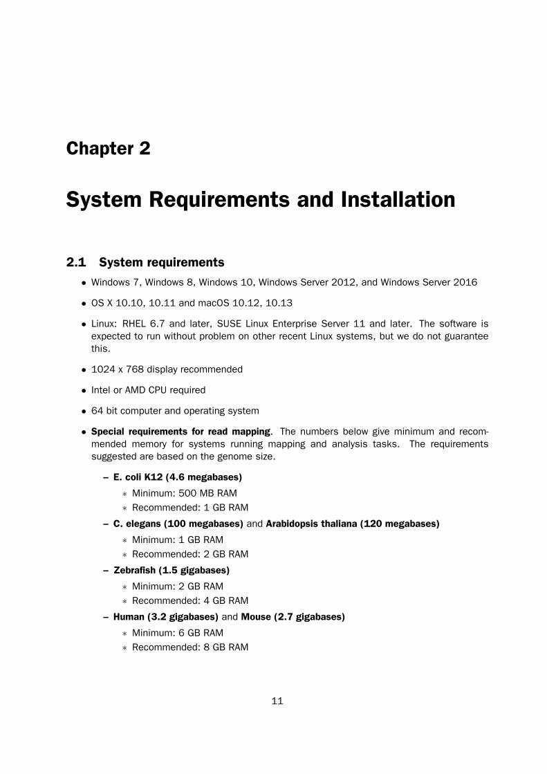
• Special requirements for read mapping. The numbers below give minimum and recom-mended memory for systems running mapping and analysis tasks. The requirementssuggested are based on the genome size.
– E. coli K12 (4.6 megabases)
∗ Minimum: 500 MB RAM∗ Recommended: 1 GB RAM
– C. elegans (100 megabases) and Arabidopsis thaliana (120 megabases)
∗ Minimum: 1 GB RAM∗ Recommended: 2 GB RAM
– Zebrafish (1.5 gigabases)
∗ Minimum: 2 GB RAM∗ Recommended: 4 GB RAM
– Human (3.2 gigabases) and Mouse (2.7 gigabases)
∗ Minimum: 6 GB RAM∗ Recommended: 8 GB RAM
11
CHAPTER 2. SYSTEM REQUIREMENTS AND INSTALLATION 12
• Special requirements for de novo assembly. De novo assembly may need more memory thanstated above - this depends both on the number of reads, error profile and the complexity andsize of the genome. See http://resources.qiagenbioinformatics.com/white-papers/White_paper_on_de_novo_assembly_4.pdf for examples of the memoryusage of various data sets.
2.1.1 Limitations on maximum number of cores
Most modern CPUs implements hyper threading or a similar technology which makes eachphysical CPU core appear as two logical cores on a system. In this manual the term "core"always refer to a logical core unless otherwise stated.
For static licenses, there is a limitation on the number of logical cores on the computer. Ifthere are more than 64 logical cores, the CLC Assembly Cell cannot be started. In this case,a network license is needed (read more at http://www.qiagenbioinformatics.com/support/licensing/).
2.1.2 Supported CPU architectures
Software from QIAGEN Aarhus is developed for and tested on the x86 and x86-64 CPU archi-tectures, which are used in most Intel and AMD CPUs. PowerPC CPUs, such as those used inApple products until 2006, are not supported. To run Assembly Cell the CPU must also supportthe SSE2 instruction set, which is commonly available in Intel CPUs produced from 2001 andonwards and AMD CPUs produced from 2003 and onwards.
If you are not sure if your CPU is supported, send a mail to [email protected] with allavailable technical information about your computer.
2.2 Disk spaceData from Next-Generation sequencing machines naturally take up a lot of disk space. Besidesthe output files, the CLC Assembly Cell will sometimes write temporary files. These files will bewritten to the directory specified in the TMP variable on Windows and TMPDIR on Linux and Mac.
2.3 Downloading and installing the software1. Download the distribution from:
https://www.qiagenbioinformatics.com/product-downloads/.
2. Unzip the zip-file and ensure that the resulting folder is placed in the desired final locationon your computer.
There are two main types of license for the CLC Assembly Cell software: static and network.Static licenses are tied to the hardware to which they are downloaded. Network licenses areserved using a separate piece of software, the CLC License Server, and allow CLC Assembly Cellprograms to run on any machine that can contact the License Server1.
1For running the software on a computer cluster, the most common license type would be a network license, whichwould then allow you to submit jobs to any node of your computer cluster.
CHAPTER 2. SYSTEM REQUIREMENTS AND INSTALLATION 13
For obtaining an evaluation license, please follow the instructions in the static license section.
2.4 Installing Static licenseFor purchased licenses, please ensure you have your License Order ID available, preferably in aform you can copy and paste, before embarking on the instructions in this section.
If you have not previously done so, you can download a 15 day evaluation license using the samelicense tool that is used to download purchased licenses.
These instructions assume that the machine you have installed CLC Assembly Cell on isconnected to the network and can access outside sites. If this is not the case, please see thesection below.
2.4.1 Licensing the software on a networked Linux or Mac machine
1. On the command line, run the clc_cell_licutil tool that you will find inside the installationdirectory of CLC Assembly Cell.
You will need to run this tool as a user that has permissions to write the license file thatis downloaded into the licenses folder in the installation directory of CLC Assembly Cell. Ifyour software is installed centrally, this may mean running the tool with sudo.
2. You will be prompted as to whether you wish to Request an evaluation license or Downloadlicense using a License Order ID.
For an evaluation license, just choose that option. As long as you have not previouslytrialled the software on your machine, the evaluation license should be downloaded. Youwill see a message printed to screen about the expiry date of the evaluation license andwhere the license was downloaded to. You should now be able to trial the software.
3. If you have a License Order ID, please copy it and then paste it in at the prompt.
After a few moments, your license should be downloaded and a message will be written to screensaying that it was successfully downloaded and where it was saved.
2.4.2 Licensing the software on a networked Windows machine
1. Go to the Windows start menu and in the search box, type cmd.
2. Click on the cmd.exe tool which will launch the windows command prompt.
You need to run this as a user that has permissions to write the license file that isdownloaded into the licenses folder in the installation directory of the CLC Assembly Cell. Ifyour software is installed centrally, this will likely mean right clicking on the cmd.exe optionand choosing to Run as administrator.
3. Navigate to the installation folder of the CLC Assembly Cell and execute the clc_cell_licutil.batscript.
4. You will be prompted as to whether you wish to Request an evaluation license or Downloadlicense using a License Order ID.
CHAPTER 2. SYSTEM REQUIREMENTS AND INSTALLATION 14
For an evaluation license, just choose that option. As long as you have not previouslytrialled the software on your machine, the evaluation license should be downloaded. Youwill see a message printed to screen about the expiry date of the evaluation license andwhere the license was downloaded to. You should now be able to trial the software.
5. If you have a License Order ID, please copy it and then paste it in at the prompt.
After a few moments, your license should be downloaded and a message will be written to screensaying that it was successfully downloaded and where it was saved.
2.4.3 Licensing the software on a non-networked machine
Using the tool distributed with CLC Assembly Cell for downloading a static license, the licensewill be specific to the machine you download it to. For a machine unable to connect to an outsidenetwork, you can follow the steps below to get a license for the software:
1. Get the host id for the machine that CLC Assembly Cell is installed on. To do this, runthe clc_cell_licutil tool as per the instructions in the Linux and Mac or Windows sectionsabove. (You do not need administrator privileges for this.)
2. Copy the Host ID(s) information that is printed near the top of the output.
3. On a machine that is able to reach external sites, go to the webpage https://secure.clcbio.com/LmxWSv3/GetLicenseFile
4. Paste in your License Order ID and your host ID information, as well as a host name. Thehost name is not important, but we recommend it is something that allows you to recogniseor identify the machine that’s been licensed if needed.
5. Click on the Save button.
6. Move the license file onto the machine where CLC Assembly Cell is installed.
7. Save the license file in the folder called licenses in the installation directory of CLCAssembly Cell2.
2.5 Network LicensesNetwork licenses are made available to users of CLC Assembly Cell software by using a separatepiece of sofware called CLC License Server.
In general terms, you need to:
• Download, install and start up CLC License Server on a machine that is accessible to themachines that CLC Assembly Cell will be running on. This would generally be a machinethat is left on, with the CLC License Server running as a service.
• Configure the license settings for copies of CLC Assembly Cell that will make use of thenetwork licenses.
2Locations for static license files supported in earlier versions of the CLC Assembly Cell can continue to beused. We recommend, however, that you choose to store your static license in the licenses folder in the installationdirectory, as this could help us in troubleshooting any licensing issues you may contact us about.

CHAPTER 2. SYSTEM REQUIREMENTS AND INSTALLATION 15
2.5.1 Installing and Running CLC License Server
How to install and run CLC License Server is described in our CLC License Server man-ual available from http://www.resources.qiagenbioinformatics.com//manuals/clclicenseserver/User_Manual.pdf.
The CLC License Server software can be downloaded from: http://www.qiagenbioinformatics.com/products/clc-license-server-direct-download/
2.5.2 Configuring the software to use a network license
In order to make CLC Assembly Cell contact the license server for a license, you need to createa text file called license.properties including the following information:
serverip=192.168.1.200serverport=6200useserver=true
The serverip and serverport should be edited to match your license server set-up.
This text file then should be placed in the licenses folder of the installation area of CLC AssemblyCell.
Locations supported in earlier versions of CLC Assembly Cell can still be used, although werecommend the location above. The full list of locations is:
• in the licenses folder of the installation area of CLC Assembly Cell.
• in the working directory
• in /etc/clcbio/licenses on the executing machine, or
• in $HOME/.clcbio/licenses/ where $HOME is the home directory of the user executing theprogram.
2.6 Restricting CPU usageDe novo assembly and mapping programs will use all cores available on the system if the jobis large enough to warrant this. Should you wish to limit the number of cores to be used by aparticular analysis, ‘--cpus’ option can be used to set the maximum.
This option is included in the full listing of options for the relevant programs.

Chapter 3
The Basics
The chapter covers the basics of command line use in CLC Assembly Cell, including data formatconsiderations such as supported data formats, the cas assembly file format and conversionto other assembly formats. The chapter ends with an overview of paired data handling in CLCAssembly Cell.
3.1 How to use the programsThe CLC Assembly Cell consists of standard command line tools, where the tool name is provided,followed by any flags or parameters required. All input to the command, including designatinginput and output files, is done via parameter arguments.
General things to be aware of when setting up a CLC Assembly Cell command include:
• For programs where there are choices between fasta and fastq as output formats, theformat that is output is determined based on the filename you specify in the command. Forexample, for the clc_remove_duplicates program, if you provide an output filename endingin .fq or .fastq, then the output format will be fastq. Otherwise, it will be fasta. Any programwith this sort of behaviour should include information about the convention used in theusage information produced by running the command without any arguments.
• When providing paired data in two files, where one file contains one member of a pairand the other file contains the other member of a pair, you must include the -i flag infront of each input file. More information is provided about this later in this chapter, whenpaired data input is discussed, as well as in the chapters on read mappings and de novoassembly.
• When providing information about sequences, such as fragment lengths, also referred toas distances, for paired data, the parameter values you enter will apply to all read filesafter that point in the command, until the point in the command where new parametervalues are provided. This is discussed further in the chapters on read mappings and denovo assembly.
3.1.1 Getting Help
This manual gives information about the tools included in CLC Assembly Cell.
16
CHAPTER 3. THE BASICS 17
Full usage information for each program is available in Appendix A of this user manual, andalso by running any of the CLC Assembly Cell commands without any arguments. For the coreprograms, clc_mapper and clc_assembler, particular parameters are discussed in more detailwithin the chapters dedicated to those tools.
3.1.2 A basic example
A basic example of a CLC Assembly Cell command would be running the clc_unpaired_readsprogram. This program generates an output file of reads that are not paired within a givenmapping. Here, we would need to specify the mapping to look at and the name of the output file.Below is an example of how such a command might look:
clc_unpaired_reads -a assembly.cas -o unmapped.fasta
3.2 Input FilesThe formats in the following table are recognized as valid input formats by one or more of the CLCAssembly Cell tools. Note that not all listed formats are valid for data to be treated as sequencereads, and not all listed formats are valid for data to be treated as reference sequences in thecase of read mappings.
Input file formats are automatically detected by the software through consideration of the filecontents. The filename is irrelevant with regards to input format.
Format Reads ReferencesFasta + +Fastq + -Scarf + -csfasta* + -Sff** + -GenBank - +
*The full sequence of any read containing one or more . symbols, present in a .csfasta formatfile, will be converted to contain only N characters when used by or output by any of the AssemblyCell tools.
**Please note that paired 454 data needs to be pre-processed using the clc_split_reads program.
Read and reference data compressed using gzip is supported as input by the CLC Assembly Cellprograms except for clc_remove_duplicates and clc_mapper_legacy.
Single reference sequences longer than 2gb (2 ·109 bases) and reads longer than 100,000 basesare not supported.
3.3 Cas File FormatCLC Assembly Cell uses the cas file format for read mappings. It is a custom file format thatcaters to the demands of high throughput sequencing data, while being flexible enough to handle
CHAPTER 3. THE BASICS 18
other sequence data types also. No deep knowledge of this file format is necessary to work withit, but some basics can aid in understanding what this format contains and how it can be used.
3.3.1 Cas Format Basics
The cas format is a binary format. This is space efficient, taking only approximately 8 bytes perread assembled to the human genome. So a cas file with 100 million Solexa reads, each with alength of 35 bases, assembled to the human genome would only take up about 800 MB.
3.3.2 What a cas file contains
In essence, cas format files contain data about the relationships between sequences in otherfiles.
In particular, cas files contain the following information:
• General info such as: program that made the file, its version and its parameters.
• The file names for the reference sequences.
• The file names for the read sequences.
• Information about the reference sequences: their number, lengths, etc.
• The scoring scheme used when making the file.
• Information about each read:
– Whether it matches anywhere.
– Which reference sequence does it match to.
– Alignment between the reference sequence and the read.
– The number of places the read matches.
– Whether the read is part of a pair.
3.3.3 What a cas file does not contain
Cas format files do not contain any sequence data. Rather than the sequence information itself,cas files contain the names of the corresponding read and reference sequence files. As sequencereads and references already exist, much space can be saved by not generating a second copyof them as part of the assembly output file.
3.3.4 Considerations and limitations
The cas file format is designed with high volume assembly data in mind. However, there arecertain considerations that should be kept in mind:
1. There is a limit of one alignment position per read. In other words, a read matching inmultiple locations can only be assigned to one of these locations within the cas file. Thislimitation is in place because when assembling short reads to a large genome, some readsmay match hundreds of thousands of locations. Keeping track of all such alignments wouldbe problematic.
CHAPTER 3. THE BASICS 19
2. If you are planning to send your assembly to someone else for viewing or further processing,you need to include your read and reference files in addition to the cas assembly file. Thisis because the cas file contains information about the assembly, and does not contain anysequence information.
3. If you are planning to send your assembly to someone else, they must put the read andreference files in the same relative location to the cas file, as you did when you ran theassembly. This is because the cas file stores relative file names, and these must matchthe location of the read and reference files when further processing is undertaken. Pleasenote though that the program change_assembly_files can be used to change the file namesand locations.
4. If you plan to convert your cas file to SAM or BAM format, which include read information,you need to have the read data used for your mapping, as well as the cas file, availablewhen you run the clc_cas_to_sam program.
3.3.5 Converting to and from SAM and BAM formats
CLC Assembly Cell includes a tool called clc_cas_to_sam to convert a cas format file to theSAM1 or BAM2 format. Also included is a tool called clc_sam_to_cas that converts from SAM orBAM format into the cas format.
These tools are described in more detail in their own sections: section 9.1 and section 9.2.
3.4 Paired read ConsiderationsYou can specify that a read file came from a paired sequencing experiment using the ‘-p’ option.This option is described in detail here, as well as within the read mapping and de novo assemblysections of the manual.
A typical set of information one would provide after the -p flag would look like this
-p fb ss 100 200
. The meaning of this would be:
• fb Specifies the relative orientation of the reads. Here, the first read of the pair is in theforward direction, the second read is in the backward, or reverse, orientation. The allowedvalues for this are provided below.
• ss Specifies the way the distances between the pair members should be measured. Here,the distances are given from the start (5 prime end) of the first read to the start (5 primeend) of the second read. Here, since the relative orientation is set to fb, the second readis reversed, so indicating ss means that the distance specified will include both the readlengths as well as the length of the sequence between the reads.
• 100 200 The range of distances expected between the specified start positions. Here thisis between 100 and 200 bases.
1Sequence Alignment/Map format2BAM is the binary compact format for SAM

CHAPTER 3. THE BASICS 20
3.4.1 Relative orientation of the reads
For all codes, it is possible to assemble the pair to any of the two reference sequence strands,so ‘ff’ may mean that both reads are placed in the forward direction or that both reads are placedin the reverse direction. There is still a difference between ‘ff’ and ‘bb’, though. For ‘bb’, thesecond read is effectively placed before the first read. The ’bb’ option is not widely used and isincluded for the sake of completeness.
The allowed values for the directions and their meanings are summarized in the table below.
ReadCode First Second Description
ff → → Both reads are forward.fb → ← Reads point toward each other.bf ← → Reads point away from each other.bb ← ← Both reads are backward.
3.4.2 Measuring the distance between the reads
How the distance between the reads should be measured depends on how the sequencingexperiment is done. If the reads are sequenced in the upstream to downstream direction, thestart of the reads is where the distance should be measured. This is indicated by the ‘ss’ codefor start to start. The allowed values are ‘ss’, ‘se’, ‘es’, and ‘ee’, where the first letter indicateswhich end of the first read should be used and the second letter indicates which end of thesecond read should be used (‘s’ for start and ‘e’ for end). The ‘ss’ option is the most typical.
So, for typical paired end Illumina sequencing protocol, using the ‘fb ss’ combination ensuresthe correct relative directions of the reads. It also ensures that the distance is independent ofthe read length since typical sequencing experiment progress expands the reads toward eachother from their starting points.
When the ‘-p’ option is used, it applies to all read files from that point and forward in thecommand line. If different experiments with different paired properties are combined, the ‘-p’option can be used several times. To indicate that the following read files are not paired, used‘-p no’. This is only necessary if another ‘-p’ option was previously used. An example:
clc_mapper -o assembly.cas -d human.gb -q reads1.fasta -p fb ss 180250 reads2.fasta -p no reads3.fasta
Here, we have three read files, where reads1.fasta and reads3.fasta are unpaired, whilereads2.fasta are paired reads.
Note that the clc_sort_pairs and clc_split_reads program can be used to convert data from SOLiDand 454 systems, respectively, into an format accepted by the CLC Assembly Cell tools.
3.4.3 Paired Read File Input
Paired data may be contained in a single file, where the pairs are sorted such that the first twosequences are one pair, the second two sequences the next pair, and so on. Paired data mayalso exist in two files, with one file containing the first member of all pairs, and the other file
CHAPTER 3. THE BASICS 21
containing the second member of all pairs, with each member appearing in the same orderedposition in each file. For example, the 51st sequence in file A is the mate of the 51st sequencein file B.
The CLC Assembly Cell programs assume the single file form for paired data as the default. Forpaired data with separate files for first and second members of the pair, both files need to beincluded as input, with each of these files being preceeded by the ‘-i’ option (for interleave). Theorder of the files on the command line matters. The first file should contain the first member ofthe pair. The second file should contain the second member of the pair.
To further illustrate this, consider a situation where we have two fasta files like this (first.fasta):
>pair_1/1ACTGTCTAGCTACTGCATTGACTGCGAC>pair_2/1TAGCGACGATGCTACTACTCTACTCGAC>pair_3/1GATCTCTAGGACTACGCTACGAGCCTCA
and this (second.fasta):
>pair_1/2GGATCATCTACGTCATCGACTAGTACAC>pair_2/2AAGCGACACCTACTCATCGATCATCAGA>pair_3/2TATCGACTCAGACACTCTATACTACCAT
where pair_1/1 and pair_1/2 belong together, pair_2/1 and pair_2/2 belong together, etc.The programs expect to see these sequences as one fasta file like this (joint.fasta):
>pair_1/1ACTGTCTAGCTACTGCATTGACTGCGAC>pair_1/2GGATCATCTACGTCATCGACTAGTACAC>pair_2/1TAGCGACGATGCTACTACTCTACTCGAC>pair_2/2AAGCGACACCTACTCATCGATCATCAGA>pair_3/1GATCTCTAGGACTACGCTACGAGCCTCA>pair_3/2TATCGACTCAGACACTCTATACTACCAT
This is accomplished using the ‘-i’ option like this:
clc_mapper -o assembly.cas -d human.gb -q -p fb ss 180 250-i first.fasta second.fasta
This is identical to:
clc_mapper -o assembly.cas -d human.gb -q -p fb ss 180 250 joint.fasta
Note that the ‘-i’ option has to immediately proceed the input files.
Chapter 4
Read Mapping
The read mapper, clc_mapper, maps a list of sequencing reads to a set of reference sequences,collectively referred to as the reference genome.
For each sequencing read, the read mapper reports the location(s) in the reference genomewhere that read is most likely to have originated from. The reported location is the result of thisprocedure:
1. A search is carried out for the longest stretches of matching bases between the referencegenome and a read by considering each base position of the read as a start position of aseed candidate.
2. End-positions of seeds are then determined by elongating the seeds as long as there arefully matching sequences in the reference index.
3. Seeds are reduced down to 2/3 of the length of the longest one.
4. Finally, the seeds are examined in detail using a banded Smith-Waterman algorithm. Seedsfrom paired reads are examined together.
The seed lengths in this mapping tool are variable, but have a minimum size of 15bp. Thevariable seed length enables identification of short seeds where the alignment score is higherthan the alignment score for longer seeds. This leads to a better mapping of some reads, andimproves the chance of identifying the optimal mapping, especially for reads with high error rates.
4.1 References and indexesThe read mapper supports mapping against a mixture of linear and circular reference sequences.
Reference sequences are typically provided in the form of one or more FASTA files1, that can bepassed to the mapper using the -d/--references parameter. Files containing sequences, tobe interpreted as circular, must be individually prefixed with the -z/--circular parameter:
clc_mapper -d linear.fa -z circular.fa linear_again.fa ...
1FASTQ is also supported.
22
CHAPTER 4. READ MAPPING 23
Internally, the provided sequences are converted into a reference index, allowing the read mapperto efficiently search and navigate them.
If you find yourself working repeatedly with the same large genomes, such as human, you cansave a lot of time by writing the index to disk using the -n/--indexoutput parameter, eg.
clc_mapper -d chr1.fa chr2.fa ... chrY.fa -z mito.fa -n human.idx ...
The next time you need to use that human reference, simply provide it as a reference:
clc_mapper -d human.idx ...
Note, that the size of the index, both on disk and in memory, is comparable to the cumulativesize of the reference sequences in FASTA format. It typically uses slightly less than one byte perbase. For example, a human index needs around 2.8 gigabytes of space.
CHAPTER 4. READ MAPPING 24
4.2 ReadsThe read mapper supports mapping both single and paired reads.
Reads are typically provided in the form of one or more FASTA or FASTQ files, that are passed tothe mapper using the -q/--reads parameter.
4.2.1 Single reads
In the case of single reads, you simply list the files after the -q/--reads parameter:
clc_mapper -q single_reads.fastq more_single_reads.fasta ...
In the special case of PacBio reads, you can optimize both quality and speed of the alignmentprocess by providing type information as follows:
clc_mapper -q --type pacbio long_pacbio_reads.fastq ...
The type, as defined by the --type parameter, applies to all following files.
4.2.2 Paired reads
Paired reads often come split across two files: one containing the first mates, paired_1.fa:
and one containing the second mates, paired_2.fa:
Use the -p/--paired parameter to indicate that the following files contain paired reads of acertain type, and use the -i/--interleave parameter to pair up the two files:
clc_mapper -q -p fb ss 50 500 -i paired_1.fa paired_2.fa ...
Behind the scenes, the pairs are interleaved and processed together:
If you have a paired file, that is already interleaved, you can leave out the -i/--interleaveparameter:
CHAPTER 4. READ MAPPING 25
clc_mapper -q -p fb ss 50 500 interleaved_pairs.fastq ...
For detailed information about the -p fb ss 50 500 parameter, please refer to 3.4.
4.3 Alignment parametersThe read mapper aligns the reads according to a user-specified scoring scheme, that expressesyour expectation of what the data looks like and guides the mapper in deciding whether aparticular alignment is good or bad.
As a rule of thumb, you want to choose a scoring scheme that matches the expected character-istics of the data. For example, if you are using a sequencing technology that has a tendency toproduce errors in the form of gaps, you may want to lower the gap cost slightly to indicate, thatgaps are expected to occur frequently.
Keep in mind, that the mapper deals with reads individually and so cannot distinguish betweenbiological events and technical errors. Since technical errors are (typically) much more likely tooccur than true genetic variation, you should set your costs according to what you expect to seein the raw reads, rather than which biological events you expect to be present in the sampleitself.
4.3.1 Match score
The -m/--matchscore parameter determines the score attributed to a pair of matching basesin an alignment (default is 1).
4.3.2 Mismatch cost
The -x/--mismatchcost parameter determines the cost incurred when a mismatch is accepted(default is 2).
4.3.3 Linear gap cost
If each base inserted or deleted is taxed independently, we have what is known as a linear gapcost model, because the total cost of a gap c(λ) is proportional to the length of the gap λ:c(λ) = gλ
where the cost per base g is set using the -g/--gapcost parameter. By default, it is set to3, but you may want to lower that, if you are mapping data from sequencing technology that isprone to produce gaps, such as Ion Torrent, PacBio, or Oxford Nanopore.
CHAPTER 4. READ MAPPING 26
If you would like to set the insertion and deletion costs differently, you can do so using acombination of the -g/--gapcost and the -e/--deletioncost parameters.
The -g/--gapcost parameter sets both the insertion and the deletion cost, while the-e/--deletioncost sets deletion cost only. For example, if you would like to set inser-tion cost to 1 and the deletion cost to 3, you would do the following:
clc_mapper ... -g 1 -e 3 ...
i.e. first set both the deletion and insertion cost to 1 and the set deletion cost back to 3.
4.3.4 Affine gap cost
If you believe that your data contains relatively few gaps, though they may be quite long, you canuse the -G/--gapopen parameter to introduce an additional penalty for opening the gap in thefirst place. This would typically be used along with a low per-base gap cost, typically 1.
In this scheme the total cost c(λ) of a gap of length λ is given by the following formula:
c(λ) = G+ gλ (4.1)
where the open cost G and the extension cost g are specified using -G and -g, respectively.Note that the affine model reduces to the linear one, when the open cost, G, is set to zero.
Using a combination of a relatively high open cost and a low extension (per-base) gap cost,indicates to the mapper that you expect few gaps, but that these may be quite long.
You should be careful about using high open costs, if you have lots of sequencing errors in theform of deletions or insertions, as these may be penalized to the point, where you get lots oflong unaligned ends. In such cases linear gap cost may be a better choice.
Like linear gap costs, affine gap costs can be used asymmetrically. This is done by independentlysetting the deletion open cost using the -E/--deletionopen parameter.
4.3.5 Alignment mode
The mapper supports two different modes of alignment: local (default) and global.
The alignment mode is set using the -a/--alignmode parameter.
In local mode, -a local, alignments are chosen to be locally optimal, i.e. the mapper looks forthe highest scoring alignment of part of the read. That is, unaligned ends are not penalized inany way.
In global mode2, -a global, the mapper is forced to look for the highest scoring alignment ofthe entire read. That is, unaligned ends are no longer free.
Generally, we recommend that you stick to local alignment, as there are several reasons, whyyou may not want to force the ends of a raw read sequence to align:
1. Read quality deteriorates towards the end of a read, so you may end up aligning noise.2This is sometimes called semi-global alignment, because the alignment is global with respect to the read, but
remains local with respect to the reference.
CHAPTER 4. READ MAPPING 27
2. If present, untrimmed adapter sequence cannot be aligned in any meaningful way.
3. Structural variation may be present in the sample, so the reference may not have corre-sponding sequence for all of the read.
In general, unaligned ends express a lack of confidence in a portion of the read; information thatcan be very helpful for several, common downstream analyses.
4.4 Reporting and filteringThe resulting alignments are output to a single CAS file3 using the -o/--output parameter:
clc_mapper -d reference.fa -q reads.fastq -o result.cas
By default, if there are multiple, equally good alignments for a particular read, the number ofalignments is stored, but detailed alignment information is only stored explicitly for one of them.Should you wish to change this behavior, you can use the following pair of parameters to do so:
The -t/--maxalign parameter determines the maximum number of alignments that are to bestored explicitly. By default, only one is stored explicitly.
The -r/--repeat parameter accepts one of two arguments: random or ignore. By default,it is set to random, which means that the explicitly stored alignments are sampled, randomly,from the total set of alignments found for a given read. The ignore argument results in readswith more alignments than can be explicitly stored are ignored and reported as unmapped.
As an example, suppose that you only want to report unique hits as mapped, i.e. ignorealignments with more than one hit. Then you can use the following combination:
clc_mapper ... -t 1 -r ignore ...
3The CAS file is a compact, binary file containing information about the alignment(s) of the individual reads. Theread and reference sequences are not stored explicitly, but rather the paths to the input files are stored.
CHAPTER 4. READ MAPPING 28
4.5 Quality filteringOnce an alignment has been found, it is examined by the quality filter. If it fails to meet thecriteria enforced by the filter, it is discarded. If all alignments of a particular read fail to meet thecriteria, the read is reported as unmapped.
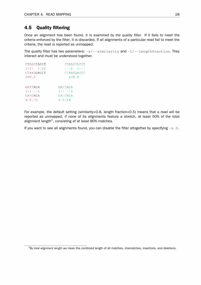
The quality filter has two parameters: -s/--similarity and -l/--lengthfraction. Theyinteract and must be understood together.
For example, the default setting (similarity=0.8, length fraction=0.5) means that a read will bereported as unmapped, if none of its alignments feature a stretch, at least 50% of the totalalignment length4, consisting of at least 80% matches.
If you want to see all alignments found, you can disable the filter altogether by specifying -s 0.
4By total alignment length we mean the combined length of all matches, mismatches, insertions, and deletions.

Chapter 5
De novo assembly
The clc_assembler program performs assembly of reads without a known reference. The inputdata consists of files containing read sequences.
5.0.1 De novo assembly inputs
Any number of read files can be input to a de novo assembly. These includes files containingpaired reads and files containing single reads. Different types of read data can be input to asingle de novo assembly. Below is a table of the accepted formats for data input.
Format optionFasta + +Fastq + -Scarf + -csfasta + -Sff * + -GenBank - +
* Please note that paired 454 data needs to be pre-processed using the clc_split_reads program
5.0.2 De novo assembly outputs
The output of the clc_assembler is a fasta file containing all the contig sequences.
This means that there is no information about where the reads are placed, how they align, cover-age levels etc. If this information is desired, you can use the clc_mapper or clc_mapper_legacyprogram and use the newly created contig sequences as references. The cas format file createdusing the mapping program will contain this sort of information.
If the -f option has been used, then a file containg features related to scaffolding will begenerated. Choosing to name the file given as an argument to the -f option with a .agp suffixwill generate an AGP format file. This format specification can be found online https://www.ncbi.nlm.nih.gov/projects/genome/assembly/agp/AGP_Specification.shtml.
Choosing to name the file given as an argument to the -f option with a .gff suffix will generate a
29
CHAPTER 5. DE NOVO ASSEMBLY 30
GFF format file. The columns of this file contain the following information:
Column 1: Name of contig Column 2: Source program Column 3: Annotation type (see below)Column 4: Start position Column 5: End position Column 6: Score (see below) Column 7, 8 and9: no meaning: there to conform to the GFF format.
Further details about Annotation types (column 3)
There are three annotation types that can appear in the third column:
1) Alternatives Excluded: More than one path through the graph was possible in this region butevidence from paired data suggested the exclusion of one or more alternative routes in favor ofthe route chosen.
2) Contigs Joined: More than one route was possible through the graph such that an unambiguouschoice of how to traverse the graph cannot by made. However evidence from paired data supportsone of these routes and on this basis, this route is followed to the exclusion of the other(s).
3) Scaffold: The route through the graph is not clear but evidence from paired data supportsthe connection of two contigs. A single contig is then reported with N characters between thetwo connected regions. This entity is also known as a scaffold. The number of N charactersrepresents the expected distance between the regions, based on the evidence the paired data.
If one chooses not to scaffold, a resulting gff annotation file will still report any "Contigs joined"and "Alternatives excluded" optimizations, as these are still performed in this case.
Further details about Scores (column 6)
For annotation type Scaffold, the size of the gap that has been estimated between scaffoldedsections of the contig is reported in the score column.
For annotation type Alternatives Excluded, the score is reported as the (word size + 1). This valuemerely serves as a reminder that the region reported for this event is associated with the wordsize used for the assembly.
For annotation type Contigs Joined, the value in the score column is 0.
5.1 How it worksOur de novo assembly algorithm works by using de Bruijn graphs. This is similar to how mostnew de novo assembly algorithms work [Zerbino and Birney, 2008,Zerbino et al., 2009,Li et al.,2010,Gnerre et al., 2011]. The basic idea is to make a table of all sub-sequences of a certainlength (called words) found in the reads. The words are relatively short, e.g. about 20 for smalldata sets and 27 for a large data set (the word size is determined automatically, see explanationbelow).
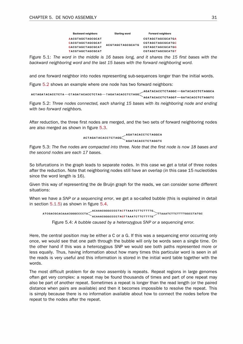
Given a word in the table, we can look up all the potential neighboring words (in all the exampleshere, word of length 16 are used) as shown in figure 5.1.
Typically, only one of the backward neighbors and one of the forward neighbors will be present inthe table. A graph can then be made where each node is a word that is present in the table andedges connect nodes that are neighbors. This is called a de Bruijn graph.
For genomic regions without repeats or sequencing errors, we get long linear stretches ofconnected nodes. We may choose to reduce such stretches of nodes with only one backward
CHAPTER 5. DE NOVO ASSEMBLY 31
Figure 5.1: The word in the middle is 16 bases long, and it shares the 15 first bases with thebackward neighboring word and the last 15 bases with the forward neighboring word.
and one forward neighbor into nodes representing sub-sequences longer than the initial words.
Figure 5.2 shows an example where one node has two forward neighbors:
Figure 5.2: Three nodes connected, each sharing 15 bases with its neighboring node and endingwith two forward neighbors.
After reduction, the three first nodes are merged, and the two sets of forward neighboring nodesare also merged as shown in figure 5.3.
Figure 5.3: The five nodes are compacted into three. Note that the first node is now 18 bases andthe second nodes are each 17 bases.
So bifurcations in the graph leads to separate nodes. In this case we get a total of three nodesafter the reduction. Note that neighboring nodes still have an overlap (in this case 15 nucleotidessince the word length is 16).
Given this way of representing the de Bruijn graph for the reads, we can consider some differentsituations:
When we have a SNP or a sequencing error, we get a so-called bubble (this is explained in detailin section 5.1.5) as shown in figure 5.4.
Figure 5.4: A bubble caused by a heterozygous SNP or a sequencing error.
Here, the central position may be either a C or a G. If this was a sequencing error occurring onlyonce, we would see that one path through the bubble will only be words seen a single time. Onthe other hand if this was a heterozygous SNP we would see both paths represented more orless equally. Thus, having information about how many times this particular word is seen in allthe reads is very useful and this information is stored in the initial word table together with thewords.
The most difficult problem for de novo assembly is repeats. Repeat regions in large genomesoften get very complex: a repeat may be found thousands of times and part of one repeat mayalso be part of another repeat. Sometimes a repeat is longer than the read length (or the paireddistance when pairs are available) and then it becomes impossible to resolve the repeat. Thisis simply because there is no information available about how to connect the nodes before therepeat to the nodes after the repeat.

CHAPTER 5. DE NOVO ASSEMBLY 32
In the simple example, if we have a repeat sequence that is present twice in the genome, wewould get a graph as shown in figure 5.5.
Figure 5.5: The central node represents the repeat region that is represented twice in the genome.The neighboring nodes represent the flanking regions of this repeat in the genome.
Note that this repeat is 57 nucleotides long (the length of the sub-sequence in the central nodeabove plus regions into the neighboring nodes where the sequences are identical). If the repeathad been shorter than 15 nucleotides, it would not have shown up as a repeat at all since theword length is 16. This is an argument for using long words in the word table. On the other hand,the longer the word, the more words from a read are affected by a sequencing error. Also, foreach extra nucleotide in the words, we get one less word from each read. This is in particular anissue for very short reads. For example, if the read length is 35, we get 16 words out of eachread if the word length is 20. If the word length is 25, we get only 11 words from each read.
To strike a balance, our de novo assembler chooses a word length based on the amount of inputdata: the more data, the longer the word length. It is based on the following:
word size 12: 0 bp - 30000 bpword size 13: 30001 bp - 90002 bpword size 14: 90003 bp - 270008 bpword size 15: 270009 bp - 810026 bpword size 16: 810027 bp - 2430080 bpword size 17: 2430081 bp - 7290242 bpword size 18: 7290243 bp - 21870728 bpword size 19: 21870729 bp - 65612186 bpword size 20: 65612187 bp - 196836560 bpword size 21: 196836561 bp - 590509682 bpword size 22: 590509683 bp - 1771529048 bpword size 23: 1771529049 bp - 5314587146 bpword size 24: 5314587147 bp - 15943761440 bpword size 25: 15943761441 bp - 47831284322 bpword size 26: 47831284323 bp - 143493852968 bpword size 27: 143493852969 bp - 430481558906 bpword size 28: 430481558907 bp - 1291444676720 bpword size 29: 1291444676721 bp - 3874334030162 bpword size 30: 3874334030163 bp - 11623002090488 bpetc.
This pattern (multiplying by 3) continues until word size of 64 which is the max. The word sizecan also be specified manually using the -w option. Using the -v (verbose) option, you can seethe word size that is automatically calculated by the assembler
5.1.1 Resolve repeats using reads
Having build the de Bruijn graph using words, our de novo assembler removes repeats and errorsusing reads. This is done in the following order:

CHAPTER 5. DE NOVO ASSEMBLY 33
• Remove weak edges
• Remove dead ends
• Resolve repeats using reads without conflicts
• Resolve repeats with conflicts
• Remove weak edges
• Remove dead ends
Each phase will be explained in the following subsections.
Remove weak edges
The de Bruijn graph is expected to contain artifacts from errors in the data. The number of readsagreeing upon an error is likely to be low especially compared to the number of reads withouterrors for the same region. When this relative difference is large enough, it’s possible to concludesomething is an error.
In the remove weak edges phase we consider each node and calculate the number c1 of edgesconnected to the node and the number of times k1 a read is passing through these edges. Anaverage of reads going through an edge is calculated avg1 = k1/c1 and then the process isrepeated using only those edges which have more than or equal avg1 reads going though it. Letc2 be the number of edges which meet this requirement and k2 the number of reads passingthrough these edges. A second average avg2 = k2/c2 is used to calculate a limit,
limit =log(avg2)
2+avg240
and each edge connected to the node which has less than or equal limit number of readspassing through it will be removed in this phase.
Remove dead ends
Some read errors might occur more often than expected, either by chance or because they aresystematic sequencing errors. These are not removed by the "Remove weak edges" phase andwill cause "dead ends" to occur in the graph, which are short paths in the graph that terminateafter a few nodes. Furthermore, the "Remove weak edges" sometimes only removes a part ofthe graph, which will also leave dead ends behind. Dead ends are identified by searching forpaths in the graph where there exits an alternative path containing four times more nucleotides.All nodes in such paths are then removed in this step.
Resolve repeats without conflicts
Repeats and other shared regions between the reads lead to ambiguities in the graph. Thesemust be resolved otherwise the region will be output as multiple contigs, one for each node inthe region.
The algorithm for resolving repeats without conflicts considers a number of nodes called thewindow. To start with, a window only contains one node, say R. We also define the border nodes

CHAPTER 5. DE NOVO ASSEMBLY 34
as the nodes outside the window connected to a node in the window. The idea is to divide theborder nodes into sets such that border nodes A and C are in the same set if there is a readgoing through A, through nodes in the window and then through C. If there are strictly more thanone of these sets we can resolve the repeat area, otherwise we expand the window.
Figure 5.6: A set of nodes.
In the example in figure 5.6 all border nodes A, B, C and D are in the same set since one canreach every border nodes using reads (shown as red lines). Therefore we expand the window andin this case add node C to the window as shown in figure 5.7.
Figure 5.7: Expanding the window to include more nodes.
After the expansion of the window, the border nodes will be grouped into two groups being set A,E and set B, D, F. Since we have strictly more than one set, the repeat is resolved by copying thenodes and edges used by the reads which created the set. In the example the resolved repeat isshown in figure 5.8.
Figure 5.8: Resolving the repeat.
The algorithm for resolving repeats without conflict can be described the following way:
1. A node is selected as the window
2. The border is divided into sets using reads going through the window. If we have multiplesets, the repeat is resolved.
CHAPTER 5. DE NOVO ASSEMBLY 35
3. If the repeat cannot be resolved, we expand the window with nodes if possible and go tostep 2.
The above steps are performed for every node.
Resolve repeats with conflicts
In the previous section repeats were resolved without excluding any reads that goes through thewindow. While this lead to a simpler graph, the graph will still contain artifacts, which have to beremoved. The next phase removes most of these errors and is similar to the previous phase:
1. A node is selected as the initial window
2. The border is divided into sets using reads going through the window. If we have multiplesets, the repeat is resolved.
3. If the repeat cannot be resolved, the border nodes are divided into sets using reads goingthrough the window where reads containing errors are excluded. If we have multiple sets,the repeat is resolved.
4. The window is expanded with nodes if possible and step 2 is repeated.
The algorithm described above is similar to the algorithm used in the previous section, exceptstep 3 where the reads with errors are excluded. This is done by calculating an averageavg1 = m1/c1 where m1 is the number of reads going through the window and c1 is the numberof distinct pairs of border nodes having one (or more) of these reads connecting them. A secondaverage avg2 = m2/c2 is calculated where m2 is the number of reads going through the windowhaving at least avg1 or more reads connecting their border nodes and c2 the number of distinctpairs of border nodes having avg1 or more reads connecting them. Then, a read between twoborder nodes B and C is excluded if the number of reads going through B and C is less than orequal to limit given by
limit =log(avg2)
2+avg216
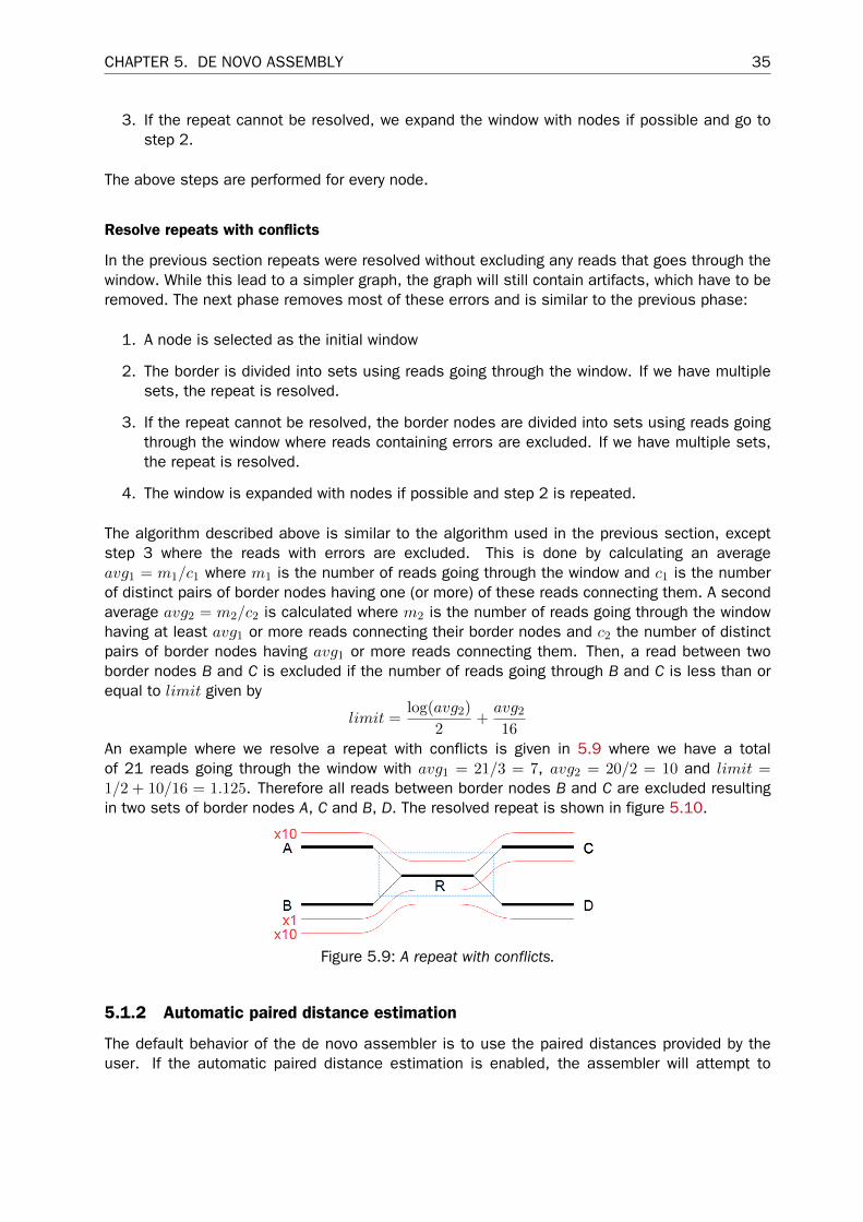
An example where we resolve a repeat with conflicts is given in 5.9 where we have a totalof 21 reads going through the window with avg1 = 21/3 = 7, avg2 = 20/2 = 10 and limit =1/2 + 10/16 = 1.125. Therefore all reads between border nodes B and C are excluded resultingin two sets of border nodes A, C and B, D. The resolved repeat is shown in figure 5.10.
Figure 5.9: A repeat with conflicts.
5.1.2 Automatic paired distance estimation
The default behavior of the de novo assembler is to use the paired distances provided by theuser. If the automatic paired distance estimation is enabled, the assembler will attempt to

CHAPTER 5. DE NOVO ASSEMBLY 36
Figure 5.10: Resolving a repeat with conflicts.
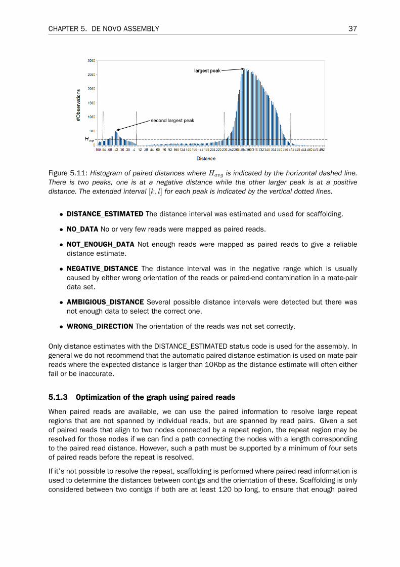
estimate the distance between paired reads. This is done by analysing the mapping of pairedreads to the long unambiguous paths in the graph which are created in the read optimizationstep described above. The distance estimation algorithm creates a histogram (H) of the paireddistances between reads in each set of paired reads (see figure 5.11). Each of these histogramsare then used to estimate paired distances as described in the following.
We denote the average number of observations in the histogram Havg =1
|H|ΣdH(d) where H(d)
is the number of observations (reads) with distance d and |H| is the number of bins in H. Thegradient of H at distance d is denoted H ′(d). The following algorithm is then used to compute adistance interval for each histogram.
• Identify peaks in H as maxi≤d≤j H(d) where [i, j] is any interval in H where {H(d) ≥Havg
2|i ≤ d ≤ j}.
• For the two largest peaks found, expand the respective intervals [i, j] to [k, l] whereH ′(k) < 0.001∧ k ≤ i∧H ′(l) > −0.001∧ j ≤ l. I.e. we search for a point in both directionswhere the number of observations becomes stable. A window of size 5 is used to calculateH ′ in this step.
• Compute the total number of observations in each of the two expanded intervals.
• If only one peak was found, the corresponding interval [k, l] is used as the distanceestimate unless the peak was at a negative distance in which case no distance estimateis calculated.
• If two peaks were found and the interval [k, l] for the largest peak contains less than 1% ofall observations, the distance is not estimated.
• If two peaks were found and the interval [k, l] for the largest peak contain <2X observationscompared to the smaller peak, the distance estimate is only computed if one peak was ata positive distance and the other was at a negative distance. If this is the case the interval[k, l] for the positive peak is used as a distance estimate.
• If two peaks were found and the largest peak has ≥2X observations compared to thesmaller peak, the interval [k, l] corresponding to the largest peak is used as the distanceestimate.
If a distance estimate for a data set is deemed unreliable, the estimate is ignored and replacedby the distance supplied by the user using the ‘-p’ option for that data set. The ‘-e’ optionrequires a file name argument ,which is used to output the result of the distance estimation foreach dataset. The output is a tab-delimited file containing the estimated distances, if any, and astatus code for each data set. The possible status codes are:
CHAPTER 5. DE NOVO ASSEMBLY 37
Figure 5.11: Histogram of paired distances where Havg is indicated by the horizontal dashed line.There is two peaks, one is at a negative distance while the other larger peak is at a positivedistance. The extended interval [k, l] for each peak is indicated by the vertical dotted lines.
• DISTANCE_ESTIMATED The distance interval was estimated and used for scaffolding.
• NO_DATA No or very few reads were mapped as paired reads.
• NOT_ENOUGH_DATA Not enough reads were mapped as paired reads to give a reliabledistance estimate.
• NEGATIVE_DISTANCE The distance interval was in the negative range which is usuallycaused by either wrong orientation of the reads or paired-end contamination in a mate-pairdata set.
• AMBIGIOUS_DISTANCE Several possible distance intervals were detected but there wasnot enough data to select the correct one.
• WRONG_DIRECTION The orientation of the reads was not set correctly.
Only distance estimates with the DISTANCE_ESTIMATED status code is used for the assembly. Ingeneral we do not recommend that the automatic paired distance estimation is used on mate-pairreads where the expected distance is larger than 10Kbp as the distance estimate will often eitherfail or be inaccurate.
5.1.3 Optimization of the graph using paired reads
When paired reads are available, we can use the paired information to resolve large repeatregions that are not spanned by individual reads, but are spanned by read pairs. Given a setof paired reads that align to two nodes connected by a repeat region, the repeat region may beresolved for those nodes if we can find a path connecting the nodes with a length correspondingto the paired read distance. However, such a path must be supported by a minimum of four setsof paired reads before the repeat is resolved.
If it’s not possible to resolve the repeat, scaffolding is performed where paired read information isused to determine the distances between contigs and the orientation of these. Scaffolding is onlyconsidered between two contigs if both are at least 120 bp long, to ensure that enough paired

CHAPTER 5. DE NOVO ASSEMBLY 38
read information is available. An iterative greedy approach is used when performing scaffoldingwhere short gaps are closed first, thus increasing the paired read information available for closinggaps (see figure 5.12).
Figure 5.12: Performing iterative scaffolding of the shortest gaps allows long pairs to be optimallyused. i1 shows three contigs with dashed arches indicating potential scaffolding. i2 is after firstiteration when the shortest gap has been closed and long potential scaffolding has been updated.i3 is the final results with three contigs in one scaffold.
Contigs in the same scaffold are output as one large contig with Ns inserted in between. Thenumber of Ns inserted correspond to the estimated distance between contigs, which is calculatedbased on the paired read information. More precisely, for each set of paired reads spanning twocontigs a distance estimate is calculated based on the supplied distance between the reads. Theaverage of these distances is then used as the final distance estimate. The distance estimate willoften be negative which happens when the paired information indicate that two contigs overlap.The assembler will attempt to align the ends of such contigs and if a high quality overlap is foundthe contigs are joined into a single contig. If no overlap is found, the distance estimate is set totwo so that all remaining scaffolds have positive distance estimates.
Furthermore, Ns can also be present in output contigs in cases where input sequencing readsthemselves contain Ns.
Please note that in CLC Genomics Workbench 6.0.1, Genomics Server 5.0.1, Assembly Cell4.0.2 and all earlier versions of these products a performance optimization gave rise to Ns beinginserted in certain non-scaffold regions, which in the current version can be solved with readscovering such specific regions.
Additional information on how paired reads have been used to in the scaffolding step can beprinted by using -f to specify an output file for GFF or AGP 2.0 formatted annotations.
The annotations in table format can be viewed by clicking the "Show Annotation Table" icon ( )at the bottom of the viewing area. "Show annotation types" in the side panel allows you to selectthe annotation "Scaffold" among a list of other annotations. The annotations tell you about thescaffolding that was performed by the de novo assembler. That is, it tells you where particularcontigs, those areas containing complete sequence information, were joined together acrossregions without complete sequence information.
For the GFF format there are three types of annotations:
• Scaffold refers to the estimated gap region between two contigs where Ns are inserted.
• Contigs joined refers to the join of two contigs connected by a repeat or another ambiguous

CHAPTER 5. DE NOVO ASSEMBLY 39
structure in the graph, which was resolved using paired reads. Can also refer to overlappingcontigs in a scaffold that were joined using an overlap.
• Alternatives excluded refers to the exclusion of a region in the graph using paired reads,which resulted in a join of two contigs.
5.1.4 AGP export
The AGP annotations describe the components that an assembly consists of. This format can bevalidated by the NCBI AGP validator.
If the exporter is executed on an assembly where the contigs have been updated using a readmapping, the N’s in some scaffolds might be resolved if you select the option "Update contigs"(figure 5.13).
Figure 5.13: Select "update contigs" by ticking the box if you want to resolve scaffolds based on aread mapping.
If the exporter encounters such a region, it will give a warning but not stop. If the exporter isexecuted on an assembly from GWB versions older than 6.5, it will often stop with an error sayingthat it encountered more than 10 N’s which wasn’t marked as a scaffold region. In this case theuser would have to rerun the assembly with GWB version 6.5 or newer of the de novo assemblerif they wish to be able to export to AGP.
Currently we output two types of annotations in AGP format:
• Contig a non-redundant sequence not containing any scaffolded regions.
• Scaffold the estimated gap region between two contigs.
5.1.5 Bubble resolution
Before the graph structure is converted to contig sequences, bubbles are resolved. As mentionedpreviously, a bubble is defined as a bifurcation in the graph where a path furcates into two nodesand then merge back into one. An example is shown in figure 5.14.
CHAPTER 5. DE NOVO ASSEMBLY 40
Figure 5.14: A bubble caused by a heteroygous SNP or a sequencing error.
In this simple case the assembler will collapse the bubble and use the route through the graphthat has the highest coverage of reads. For a diploid genome with a heterozygous variant, therewill be a fifty-fifty distribution of reads on the two variants, and this means that the choice of oneallele over the other will be arbitrary. If heterozygous variants are important, they can be identifiedafter the assembly by mapping the reads back to the contig sequences and performing standardvariant calling. For random sequencing errors, it is more straightforward; given a reasonable levelof coverage, the erroneous variant will be suppressed.
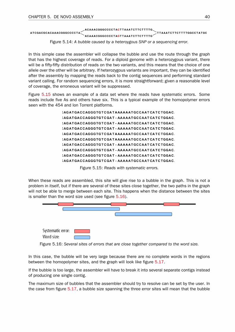
Figure 5.15 shows an example of a data set where the reads have systematic errors. Somereads include five As and others have six. This is a typical example of the homopolymer errorsseen with the 454 and Ion Torrent platforms.
Figure 5.15: Reads with systematic errors.
When these reads are assembled, this site will give rise to a bubble in the graph. This is not aproblem in itself, but if there are several of these sites close together, the two paths in the graphwill not be able to merge between each site. This happens when the distance between the sitesis smaller than the word size used (see figure 5.16).
Figure 5.16: Several sites of errors that are close together compared to the word size.
In this case, the bubble will be very large because there are no complete words in the regionsbetween the homopolymer sites, and the graph will look like figure 5.17.
If the bubble is too large, the assembler will have to break it into several separate contigs insteadof producing one single contig.
The maximum size of bubbles that the assembler should try to resolve can be set by the user. Inthe case from figure 5.17, a bubble size spanning the three error sites will mean that the bubble
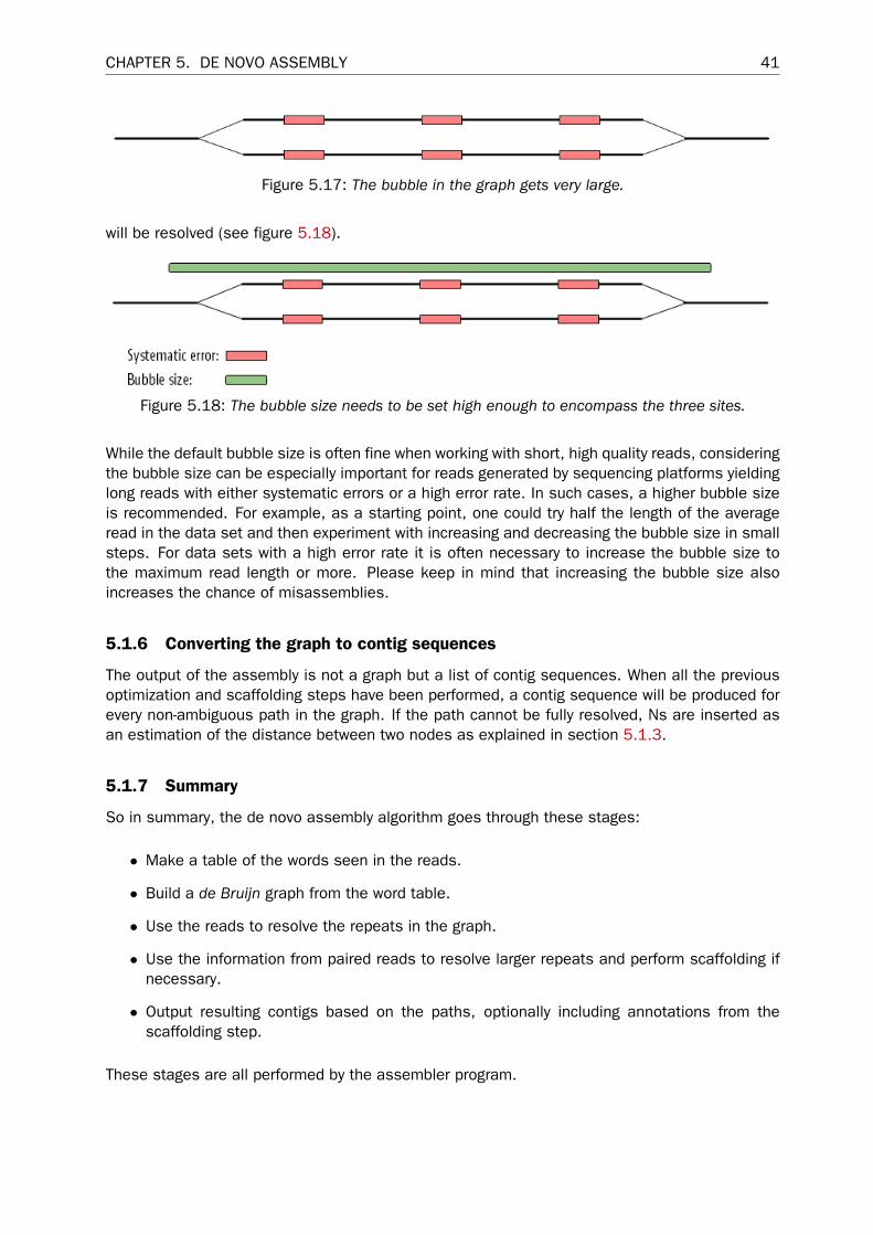
CHAPTER 5. DE NOVO ASSEMBLY 41
Figure 5.17: The bubble in the graph gets very large.
will be resolved (see figure 5.18).
Figure 5.18: The bubble size needs to be set high enough to encompass the three sites.
While the default bubble size is often fine when working with short, high quality reads, consideringthe bubble size can be especially important for reads generated by sequencing platforms yieldinglong reads with either systematic errors or a high error rate. In such cases, a higher bubble sizeis recommended. For example, as a starting point, one could try half the length of the averageread in the data set and then experiment with increasing and decreasing the bubble size in smallsteps. For data sets with a high error rate it is often necessary to increase the bubble size tothe maximum read length or more. Please keep in mind that increasing the bubble size alsoincreases the chance of misassemblies.
5.1.6 Converting the graph to contig sequences
The output of the assembly is not a graph but a list of contig sequences. When all the previousoptimization and scaffolding steps have been performed, a contig sequence will be produced forevery non-ambiguous path in the graph. If the path cannot be fully resolved, Ns are inserted asan estimation of the distance between two nodes as explained in section 5.1.3.
5.1.7 Summary
So in summary, the de novo assembly algorithm goes through these stages:
• Make a table of the words seen in the reads.
• Build a de Bruijn graph from the word table.
• Use the reads to resolve the repeats in the graph.
• Use the information from paired reads to resolve larger repeats and perform scaffolding ifnecessary.
• Output resulting contigs based on the paths, optionally including annotations from thescaffolding step.
These stages are all performed by the assembler program.
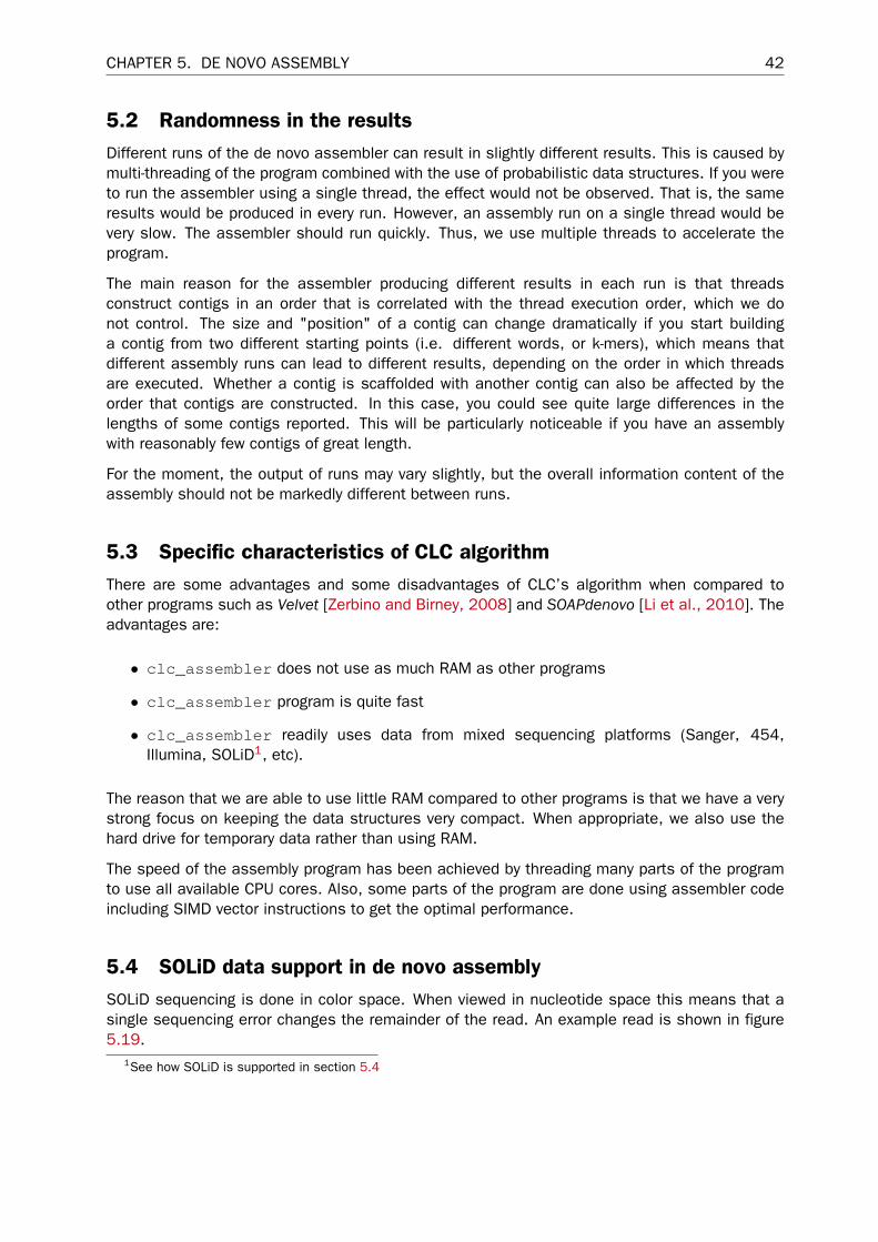
CHAPTER 5. DE NOVO ASSEMBLY 42
5.2 Randomness in the resultsDifferent runs of the de novo assembler can result in slightly different results. This is caused bymulti-threading of the program combined with the use of probabilistic data structures. If you wereto run the assembler using a single thread, the effect would not be observed. That is, the sameresults would be produced in every run. However, an assembly run on a single thread would bevery slow. The assembler should run quickly. Thus, we use multiple threads to accelerate theprogram.
The main reason for the assembler producing different results in each run is that threadsconstruct contigs in an order that is correlated with the thread execution order, which we donot control. The size and "position" of a contig can change dramatically if you start buildinga contig from two different starting points (i.e. different words, or k-mers), which means thatdifferent assembly runs can lead to different results, depending on the order in which threadsare executed. Whether a contig is scaffolded with another contig can also be affected by theorder that contigs are constructed. In this case, you could see quite large differences in thelengths of some contigs reported. This will be particularly noticeable if you have an assemblywith reasonably few contigs of great length.
For the moment, the output of runs may vary slightly, but the overall information content of theassembly should not be markedly different between runs.
5.3 Specific characteristics of CLC algorithmThere are some advantages and some disadvantages of CLC’s algorithm when compared toother programs such as Velvet [Zerbino and Birney, 2008] and SOAPdenovo [Li et al., 2010]. Theadvantages are:
• clc_assembler does not use as much RAM as other programs
• clc_assembler program is quite fast
• clc_assembler readily uses data from mixed sequencing platforms (Sanger, 454,Illumina, SOLiD1, etc).
The reason that we are able to use little RAM compared to other programs is that we have a verystrong focus on keeping the data structures very compact. When appropriate, we also use thehard drive for temporary data rather than using RAM.
The speed of the assembly program has been achieved by threading many parts of the programto use all available CPU cores. Also, some parts of the program are done using assembler codeincluding SIMD vector instructions to get the optimal performance.
5.4 SOLiD data support in de novo assemblySOLiD sequencing is done in color space. When viewed in nucleotide space this means that asingle sequencing error changes the remainder of the read. An example read is shown in figure5.19.
1See how SOLiD is supported in section 5.4
CHAPTER 5. DE NOVO ASSEMBLY 43
Figure 5.19: How an error in color space leads to a phase shift and subsequent problems for therest of the read sequence
Basically, this color error means that C’s become A’s and A’s become C’s. Likewise for G’s andT’s. For the three different types of errors, we get three different ends of the read. Along withthe correct reads, we may get four different versions of the original genome due to errors. So ifSOLiD reads are just regarded in nucleotide space, we get four different contig sequences withjumps from one to another every time there is a sequencing error.
Thus, to fully accommodate SOLiD sequencing data, the special nature of the technology has tobe considered in every step of the assembly algorithm. Furthermore, SOLiD reads are fairly shortand often quite error prone. Due to these issues, we have chosen not to include SOLiD support inthe first algorithm steps, but only use the SOLiD data where they have a large positive effect onthe assembly process: when applying paired information. Thus, the clc_assembler programhas a special option ("-p d") to indicate that a certain data set should be used only for its pairedinformation. This option should always be applied to SOLiD data. It is also useful for data setsof other types with many errors. The errors might have the effect of confusing the initial graphbuilding more than improving it. But the paired information is still valuable and can be used withthis option.
5.5 Command line optionsThis section provides details of the command line options available for the clc_assemblercommand. As with all other programs in the CLC Assembly Cell, full usage information are givenin Appendix A and can be viewed by executing the command without any arguments.
Note that you can use the clc_sequence_info program with the ‘-n’ option to get statisticson the result of a de novo assembly. This is described in the Viewing and reporting tools sectionof the manual.
5.5.1 Specifying the data for the assembly and how it should be used
The parameters described in this section can be used multiple times within a single clc_assemblercommand.
Information provided using flags that can be specified multiple times in a single commandpertains to all inputs that follow until you specify otherwise. For example, if you state you wishreads to be used for guidance only, all datasets entered via the command from that point forwardwill be used only for guidance, until a point in the command where you choose to indicate thatreads should be used at all stages of the assembly. Please see the examples section below forfurther details on this.
Some of these options are most easily explained by considering the de novo as consisting offour steps:
1. Create fragments from reads.

CHAPTER 5. DE NOVO ASSEMBLY 44
2. Connect fragments based on all reads to form a graph.
3. Optimize the graph based on all reads.
4. Optimize the graph based on paired reads.
-p <par> / --paired <par>
Here, par is a set of parameters, which indicate the pair status of your data, and for paired data,the relative orientations and expected distances between members of the pair. Options after the-p flag are also used to indicate if paired data are in two files and also whether any particular datashould be used only for its paired distance information during the final phase of the assembly.
Paired status
Data are assumed to be paired by default. To indicate that the data contain single reads, thatis, that the data are not paired, the single string value "no" is given. I.e. "-p no" followed by thename of the read file.
Paired information
For paired data, par consists of four strings: <mode> <distance_mode> <min_dist> <max_dist>
mode indicates the relative orientation of the reads in a pair set. These can be ff, fb, bf or bb.These are used for "forward-forward" reads, "forward-reverse" reads, "reverse-forward" readsand "reverse-reverse" reads2.
distance_mode indicates the point on paired reads from which the distance measure youprovide is taken. The options are ss, se, es or ee. These mean "start-start", "start-end" reads,"end-start" reads and "end-end".
<min_dist> and <max_dist> give the minimum and maximum distance range for thedistances between the pairs. Where to take the start and end points of this distance range iswhat is specified by the distance_mode described above.
So, -p fb ss 180 250 would indicate that the reads are inverted and pointing towards eachother, that the distance range includes the sequences of both the reads as well as the fragmentbetween them, and that the distance range is between 180 and 250 bases.
How data should be used in the assembly
-p d <mode> <distance_mode> <min_dist> <max_dist> An additional option, d, canbe added to the -p flag to indicate that the reads should only be used in the fourth step of theassembly, as listed at the top of this section. That is, the paired distance information associatedwith these reads is used when optimizing the graph. The sequence information itself is not usedtowards the assembly result. This is useful for data such as SOLiD, where the reads are quiteshort and may contain many errors. Such reads would not, by themselves, be of great help inbuilding and optimizing the graph initially, but the paired information associated with them canbe valuable during the final graph optimization stage.
Please also refer to the information about the -g option in the section below.
-g <mode>/ --fragmentmode <mode>
2The letter "b" in the mode strings refers to the word "backwards", but the more common word to use to describethis relative orientation is "reverse".
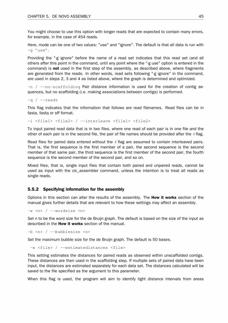
CHAPTER 5. DE NOVO ASSEMBLY 45
You might choose to use this option with longer reads that are expected to contain many errors,for example, in the case of 454 reads.
Here, mode can be one of two values: "use" and "ignore". The default is that all data is run with-g ’use’.
Providing the "-g ignore" before the name of a read set indicates that this read set (and allothers after this point in the command, until any point where the "-g use" option is entered in thecommand) is not used in the first step of the assembly, as described above, where fragmentsare generated from the reads. In other words, read sets following "-g ignore" in the command,are used in steps 2, 3 and 4 as listed above, where the graph is determined and optimized.
-n / --no-scaffolding Pair distance information is used for the creation of contig se-quences, but no scaffolding (i.e. making associations between contigs) is performed.
-q / --reads
This flag indicates that the information that follows are read filenames. Read files can be infasta, fastq or sff format.
-i <file1> <file2> / --interleave <file1> <file2>
To input paired read data that is in two files, where one read of each pair is in one file and theother of each pair is in the second file, the pair of file names should be provided after the -i flag.
Read files for paired data entered without the -i flag are assumed to contain interleaved pairs.That is, the first sequence is the first member of a pair, the second sequence is the secondmember of that same pair, the third sequence is the first member of the second pair, the fourthsequence is the second member of the second pair, and so on.
Mixed files, that is, single input files that contain both paired and unpaired reads, cannot beused as input with the clc_assembler command, unless the intention is to treat all reads assingle reads.
5.5.2 Specifying information for the assembly
Options in this section can alter the results of the assembly. The How it works section of themanual gives further details that are relevant to how these settings may affect an assembly.
-w <n> / --wordsize <n>
Set n to be the word size for the de Bruijn graph. The default is based on the size of the input asdescribed in the How it works section of the manual.
-b <n> / --bubblesize <n>
Set the maximum bubble size for the de Bruijn graph. The default is 50 bases.
-e <file> / --estimatedistances <file>
This setting estimates the distances for paired reads as observed within unscaffolded contigs.These distances are then used in the scaffolding step. If multiple sets of paired data have beeninput, the distances are estimated separately for each data set. The distances calculated will besaved to the file specified as the argument to this parameter.
When this flag is used, the program will aim to identify tight distance intervals from areas

CHAPTER 5. DE NOVO ASSEMBLY 46
containing a substantial number of the mapped reads for each dataset.
There are situations where it is not possible to estimate accurate paired distances from the data,such as:
• No best candidate interval for distance estimation can be specified as the two bestcandidate intervals to be used for estimating the distances differ only by a factor of two inthe number of pairs they contain.
• The best interval suggests a negative average distance for the paired reads in a dataset.
• More than half the reads have the wrong relative orientation.
• The best interval contains less than 1% of the mapped reads in that dataset.
If it is not possible to estimate an accurate distance from the data for any particular paired readset, then the original paired distance entered as part of the parameter settings associated withthe -p flag will be used. Errors and warnings associated with such situations will be written tothe file specified with the -e parameter.
5.5.3 Specifying information about the outputs
-o <file> / --output <file> Give the name for the file that will contain the contigs, infasta format, that are assembled.
This parameter is required.
-m <n> / --min-length <n> Set the minimum length for contigs to be output from theassembly process. The default value is 200 bases.
-f <file> / --feature_output <file>
Providing this option indicates that the annotations associated with scaffolding should be output.
The output can be in GFF format (the default), or in AGP format. The file suffix you providespecifies the output format. For AGP format, use ’.agp’. For gff format, you can use whatevername you like, but it would be usual to use the filename suffix ’.gff’.
5.5.4 Other options
--cpus <n> Specify the maximum number of cpus that should be used by the assemblyprocess. If not set explicitly, the process assumes it has access to as much of your computer’scpus as it needs.
-v / --verbose: This option specifies that verbose reporting should be turned on. Thisresults in various information being written to the terminal when the process is running, includethe word size used if you have chosen to allow that to be determined by the assembly program.
5.5.5 Example commands
The command below is a mixed assembly, where a set of paired reads, available in two fileswith one member of each pair in each file, is used for all stages of the assembly, and a set of
CHAPTER 5. DE NOVO ASSEMBLY 47
454 data is used for guidance only. The output file, containing the fasta formatted assembledcontigs, will be called myContigs.fasta.
Note the use of the -p no before the non-paired, 454 data. This ensures that the assemblerknows that the data about to be entered are not paired. It effectively overwrites the earlier -pinformation provided earlier in the command.
clc_assembler -o myContigs.fasta -p fb ss 200 400 -q -i pairedRead-member1.fastqpairedRead-member2.fastq -g ignore -p no -q 454read.sff
The above command is equivalent to:
clc_assembler -o myContigs.fasta -g ignore -p no -q 454read.sff -g use-p fb ss 200 400 -q -i pairedRead-member1.fastq pairedRead-member2.fastq
Examples of undesirable commands
A command like the following would imply that the data in 454reads. sff was paired, inan interleaved file, with the reads having relative orientation of forward-reverse, and a paireddistance range of 200 to 400 bases. That is, the earlier information provided to the -p parameterwould be used for all the following data entered in the command.
clc_assembler -o myContigs.fasta -p fb ss 200 400 -q -i pairedRead-member1.fastqpairedRead-member2.fastq -g ignore -q 454read.sff
A command like the following would fail because all reads are now used in a guidance only role.This leaves no reads being used to create the graph fragments in the initial stage. The reasonhere is that the -g ignore parameter is given early in the command and because not -g useparameter is entered later, all read sets are ignored for the building of the fragments.
clc_assembler -o myContigs.fasta -g ignore -p no -q 454read.sff -p fb ss 200 400 -q-i pairedRead-member1.fastq pairedRead-member2.fastq
CHAPTER 5. DE NOVO ASSEMBLY 48
5.6 New long read assembly tools (beta)The purpose of the last three sections in this chapter on de novo assembly is to introduce twonew tools that we have made specifically to assist with long read assembly. Note that both toolsare still considered beta quality, and that they have exclusively been tested with PacBio data.
The two tools work in tandem:
• The clc_correct_pacbio_reads tool (optionally) error-corrects PacBio reads, leadingto a much improved subsequent PacBio assembly.
• The clc_assembler_long is our long read de novo assembler.
In the next two subsections, we will show you how to use the two tools.
5.7 The clc_correct_pacbio_reads tool (beta)The clc_correct_pacbio_reads tool performs error-correction of PacBio reads.
IMPORTANT NOTICE: This tool relies on certain methods that are the intellectual property ofPacific Biosciences. Consequently, the use of this tool with any data other than data generatedon a Pacibic Biosciences instrument constitutes a violation of the end-user license agreementthat users of the CLC Assembly Cell agree to during installation.
A typical PacBio run produces a wide range of different read lengths. All other things being equal,the longer a read is, the more useful it is for de novo assembly. The primary reason for this is theability of long reads to span longer repeats and connect with more unique sequence surroundingthe repeat, clearly delimiting that repeat region in the final assembly.
Raw PacBio reads exhibit a much higher rate of (random) errors than short read technologies,such as Illumina. Unaddressed, this added noise would confuse the assembler, leading to a poorassembly.
The clc_correct_pacbio_reads tool performs optional, but highly recommended, pre-processing of the raw reads that alleviates this problem. It takes as input the raw reads andproduces a new FASTA file3 containing error-corrected versions of those long reads.
The error correction itself is a step-wise process. Somewhat simplified, it consists of three steps:
• Step 1. The raw reads are split into two classes: long reads (or seed reads) and shortreads (or correction reads). The way the split is made is governed by the --fractionparameter. By default, the longest reads, corresponding to 30% of the total read length,become the seed reads.
• Step 2. The short reads are then mapped against the long reads. Typically, several shortreads end up covering each position of the long read.
• Step 3. Finally, each long read is considered along with the corresponding short reads toform a consensus sequence by per-position majority vote. Because the noise in the rawsequences is close to random, much of that noise is eliminated by this process, and wecan consider the consensus sequence a corrected version of the read.
3The corrected reads will not have quality scores, as it is unclear how to calculate these in any meaningful way.However, this is not a problem, as quality scores are not used in the subsequent assembly process.
CHAPTER 5. DE NOVO ASSEMBLY 49
5.7.1 Interlude: Converting PacBio’s BAM to FASTA
PacBio reads are now output from their sequencing instruments in BAM format (http://pacbiofileformats.readthedocs.org/en/3.0/BAM.html). As our tools only work withFASTA or FASTQ, we recommend that you convert the reads to FASTA format using samtools(https://github.com/samtools/samtools). Once you have samtools up and running, thefollowing command does the trick:
samtools fasta -0 raw_reads.fa original_pacbio_reads.bam
5.7.2 Basic usage
To specify the raw input reads, use the -q/--reads parameter followed by one or more FASTAor FASTQ files.
The resulting corrected reads are output to a FASTA file whose name is specified after the-o/--output parameter.
5.7.3 Advanced parameters
We currently expose four parameters that allow you to tweak the behavior of the algorithm.
As briefly mentioned above, you can use the -f/--fraction parameter (default value is 30) tocontrol how the distinction between long reads and short reads is made. By default, the longestreads corresponding to 30% of the total read length are considered "long".
Once all the short reads have been mapped to the long reads, you have the option of adjustingthree filtering criteria. If short-on-long coverage falls beneath the value provided after the-m/--min-coverage parameter, those parts of the corrected long read are excised, resultingin several, shorter reads. Those shorter reads are then filtered according to the following twoparameters:
• The -l/--min-read-length parameter allows you to set a minimum read length (defaultis 1000). Corrected reads shorter than this are discarded.
• The -a/--min-average-coverage parameter specifies a lower bound on the averagecoverage across a corrected read (default is 15). If a read’s average coverage is lower, thatread will be discarded.
Here is a complete example, where we correct the PacBio reads contained in raw_reads.faand, producing a single file containing the corrected long reads corrected_reads.fa:
clc_correct_pacbio_reads -q raw_reads.fa -o corrected_reads.fa-f 30 -m 10 -l 1000 -a 15
5.8 The clc_assembler_long tool (beta)In this section we give a brief introduction to the new long read assembler.

CHAPTER 5. DE NOVO ASSEMBLY 50
We discuss the method employed, basic usage, and provide a complete example including errorcorrection for PacBio reads.
Note that the long read assembler was designed to be used for the assembly of microbialgenomes and small eukaryotic genomes.
5.8.1 Method
Like our old assembler, the long read assembler builds a kind of de Bruijn graph to do theassembly.
Since the method is k-mer based, a (fixed) word size k, should be chosen and provided to theassembler using the -w/--wordsize parameter. If left out, the assembler will do its best todecide on a word size based on the size of the input data.
When the assembler is run, we first count all the k-mers occurring in the reads, provided asone or more FASTA or FASTQ files containing the reads. The k-mers are identified with theirreverse-complements as we have no way of knowing which strand gave rise to a particular read.
Once all the k-mers have been counted, we throw away all k-mers that occur fewer than auser-specified number of times, since unique, or rarely occurring, k-mers can often be attributedto sequencing errors.
In the next step, any k-mers that always occur next to each other, i.e. only have k − 1 overlapwith one another, are joined together, iteratively, into longer fragments4.
Next, we do a second pass through the read data; mapping all the reads back to the fragments.Reads that span/link multiple fragments give rise to connections between the fragments, andtogether, the fragments (nodes) and those connections (edges) form a graph structure. If thereis a gap between two fragments, that gap is replaced by a majority consensus sequence of thereads spanning it.
From this point, the assembly graph represents our knowledge of the genome that we aim toassemble. However, it is often a very messy graph, and it is not immediately possible to readoff the chromosome, or chromosomes, that we are trying to assemble. Luckily, we have a lot ofinformation available, such as information about how well the individual edges are supported. Weuse this information along with the graph topology itself to reduce noise and tease out the actualinformation content of the graph. This simplification process consists of many, quite technical,steps and will not be covered in any detail here.
Once the graph has been simplified into a number of longer contigs, as an optional step, it ispossible to polish the contigs by mapping the reads back onto the contigs, replacing them withthe respective consensus sequences. In the case of error-corrected PacBio reads, you will getthe best result by using the original raw reads, instead of the error-corrected ones, to do thepolishing.
Finally, the resulting assembly/contigs are output to a FASTA file.
4Given a set of reads, word size k, and minimum coverage c; the resulting fragments are unambiguously defined.
CHAPTER 5. DE NOVO ASSEMBLY 51
5.8.2 Input parameters
The input reads must be provided as one or more FASTA or FASTQ files following the -q/--readsparameter.
5.8.3 Graph construction
We expose two optional parameters that greatly influence the way the fragments, and subse-quently the assembly graph, gets constructed.
The -w/--wordsize parameter allows you to set the fixed k-mer length used during fragmentconstruction. If left out, the assembler tries to estimate a reasonable word size k based on thenumber of bases in the input data.
The -c/--min-coverage parameter specifies a lower bound on the number of times, we wantto see any given k-mer for it to play a part in fragment construction (default 3).
Should you want to inspect the resulting fragments, you can choose to save them to a FASTA fileusing the -f/--savefragments parameter.
You also have the option of saving the constructed graph using the --savegraph parameter.That way you can experiment with different post-processing steps without continuously rebuildingthe graph. Afterwards, you simply reuse the graph by adding the --loadgraph parameter insubsequent runs.
5.8.4 Graph post-processing
The -a/--anchor-length specifies a minimum length for fragments to become part of thefinal assembly graph (default 100). Raising this helps to eliminate entangled, noisy structures inthe graph. On the flip side, you may need a lower value to correctly resolve complex regions.
5.8.5 Contig post-processing
As explained above, you can polish the final contigs by mapping the reads back to them, replacingthem with the resulting consensus sequence. If you want to do this, simply provide the read file,or files, to use for polishing following the -r/--polishingreads parameter.
5.8.6 Output parameters
As the output of the assembly process is a number of contigs/sequences, you must providethe name of the FASTA file they should be written to. This is done using the -o/--outputparameter.
If you want to filter out short contigs before they are written to the output file, you can specify acut-off using the -m/--min-length parameter (default 500). Contigs below that length will notbe output.

CHAPTER 5. DE NOVO ASSEMBLY 52
5.8.7 An example including error-correction for PacBio reads
Say we start out having a BAM file with raw reads from a PacBio instrument, raw_reads.bam.First thing we need to do is extract the reads in FASTA format using samtools:
samtools fasta -0 raw_reads.fa raw_reads.bam
We now have the reads in the FASTA file raw_reads.fa and will no longer be needing theoriginal BAM file.
Next, we error-correct the raw PacBio reads:
clc_correct_pacbio_reads -q raw_reads.fa -o corrected_reads.fa
We are now ready to start the assembly. We want to use the corrected reads (corrected_reads.fa)for the assembly itself and use the raw reads (raw_reads.fa) for polishing.
clc_assembler_long -q corrected_reads.fa -r raw_reads.fa -o contigs.fa
Let us assume that we have inspected the result in contigs.fa and are unhappy with thequality of the result; perhaps we would like to see fewer contigs or would like a total contiglength closer to that of our expected genome length. We can then re-run the same assembly withslightly different parameters and opt to save the graph, in case we need to do more runs:
clc_assembler_long -q corrected_reads.fa -r raw_reads.fa -o contigs.fa--min-coverage 4 --savegraph raw_reads.graph
Say we inspect the result again and are still not quite happy. Maybe we want to raise the anchorlength because we expect there to be some unwanted noise in the graph. Because we havesaved the graph, we can cut run-time significantly on this run by re-loading the saved graph:
clc_assembler_long -q corrected_reads.fa -r raw_reads.fa -o contigs.fa--min-coverage 4 --loadgraph raw_reads.graph--anchor-length 200
If the data is good and the sample genome is tractable, we should end up with a decent resultafter a few iterations of this procedure.
Chapter 6
Reporting tools
6.1 The clc_sequence_info ProgramThe clc_sequence_info program gives some basic information about the sequences in a fastafile:
File data/paired.fasta
Number of sequences 47356
Residue counts:Total 11114027
Sequence length:Minimum 170Maximum 240Average 234.69
Using the ‘-r’ options include counts of the different types of nucleotides, with all ambiguousnucleotides counted as N’s. The ‘-a’ option used together with the ‘-r’ option does the counts foramino acids.
The lengths of the sequences can be printed or summarized using the ‘-l’ and ‘-k’ options,respectively.
It is also possible to get various sequence length statistics. Using the ‘-n’ option, the N50 valueof the sequences is calculated. The N50 value means that the sum of sequences of this lengthor longer is at least 50% of the total length of all sequences. This is useful to get a quick qualityoverview of a de novo assembly.
Use the ‘-c’ option to disregard all sequences under a certain length from being considered inthe statistics. This is sometimes useful for analyzing de novo assembly results, where shortsequences may not be of interest.
Further details are available in Appendix A.
53
CHAPTER 6. REPORTING TOOLS 54
6.2 The clc_mapping_table ProgramThe clc_mapping_table program takes a single cas file as input and prints assembly informationfor each read. By default, clc_mapping_table makes a table with one read per row. The columnsare:
• Read number (starting from 0).
• Read name (enable using the ‘-n’ option).
• Read length.
• Read position for alignment start.
• Read position for alignment end.
• Reference sequence number (starting from 0).
• Reference position for alignment start.
• Reference position for alignment end.
• Whether the read is reversed (0 = no, 1 = yes).
• Number of optimal locations for the read.
• Alignment score (enable using the ‘-s’ option).
If a read does not match, all columns except the read number and name are ‘-1’. If a read isreverse, the read positions for the alignment start and end are given after the reversal of theread. The sequence positions start from 0 indicating before the first residue and end at thesequence length indicating after the last residue. So a read of length 35, which matches perfectlywill have an alignment start position of 0 and an alignment end position of 35.
Here is part of an example output using both the ‘-n’ and the ‘-s’ option:
208 SLXA-EAS1_89:1:1:622:715/1 35 0 35 0 89385 89420 0 1 35209 SLXA-EAS1_89:1:1:622:715/2 35 0 35 0 89577 89612 1 1 35210 SLXA-EAS1_89:1:1:201:524/1 35 0 32 0 4829 4861 0 1 29211 SLXA-EAS1_89:1:1:201:524/2 -1 -1 -1 -1 -1 -1 -1 -1 -1212 SLXA-EAS1_89:1:1:662:721/1 35 0 35 0 38254 38289 1 1 35213 SLXA-EAS1_89:1:1:662:721/2 35 0 35 0 38088 38123 0 1 32214 SLXA-EAS1_89:1:1:492:826/1 35 0 35 0 81872 81907 1 1 35215 SLXA-EAS1_89:1:1:492:826/2 35 0 35 0 81685 81720 0 1 35
As the read names indicate, the data are from a paired experiment. Read 211 does not matchat all and only the first 32 out of the 35 positions in read 210 matches. The score for this readis 29, indicating that a mismatch is also present (31 - 2 = 29). Read 213 also has a mismatchwhile the rest of the sequences match perfectly. We can also see that the pairs are located closetogether and on opposite strands.
Use the ‘-a’ option to get a very detailed output (‘-n’ and ‘-s’ are without effect here):
SLXA-EAS1_89:1:1:622:715/1 has 1 match with a score of 35:

CHAPTER 6. REPORTING TOOLS 55
89385 TTGCTGTGGAAAATAGTGAGTCATTTTAAAACGGT 89419 coli|||||||||||||||||||||||||||||||||||TTGCTGTGGAAAATAGTGAGTCATTTTAAAACGGT read
SLXA-EAS1_89:1:1:622:715/2 has 1 match with a score of 35:
89577 AAACTCCTTTCAGTGGGAAATTGTGGGGCAAAGTG 89611 coli|||||||||||||||||||||||||||||||||||AAACTCCTTTCAGTGGGAAATTGTGGGGCAAAGTG reverse read
SLXA-EAS1_89:1:1:201:524/1 has 1 match with a score of 29:
4829 ATCCAGGCGAATATGGCTTGTTCCTCGGCACC 4860 coli||||||||||||||||||| ||||||||||||ATCCAGGCGAATATGGCTTTTTCCTCGGCACCCCG read
SLXA-EAS1_89:1:1:201:524/2 has 0 matches
SLXA-EAS1_89:1:1:662:721/1 has 1 match with a score of 35:
38254 AGGGCATTCGATACGGTGGATAAGCTGAGTGCCTT 38288 coli|||||||||||||||||||||||||||||||||||AGGGCATTCGATACGGTGGATAAGCTGAGTGCCTT reverse read
SLXA-EAS1_89:1:1:662:721/2 has 1 match with a score of 32:
38088 ACTGAGTGATTGATTCGCGAGCCACATACTGTGGA 38122 coli|||||||||||||||||||||||||||||| ||||ACTGAGTGATTGATTCGCGAGCCACATACTCTGGA read
SLXA-EAS1_89:1:1:492:826/1 has 1 match with a score of 35:
81872 GCATCCAGCACTTTCAGCGCCTGGGTCATCACTTC 81906 coli|||||||||||||||||||||||||||||||||||GCATCCAGCACTTTCAGCGCCTGGGTCATCACTTC reverse read
SLXA-EAS1_89:1:1:492:826/2 has 1 match with a score of 35:
81685 TTCTGGTTGCTGGTCTGGTGGTAAATGTTCCCACT 81719 coli|||||||||||||||||||||||||||||||||||TTCTGGTTGCTGGTCTGGTGGTAAATGTTCCCACT read
Note! The positions in the standard output assumes the reference sequence starts at 0.However, the ‘-a’ option assumes that the reference starts at 1. This is due to the fact thatthe ‘-a’ option is intended to produce human-readable output whereas the standard option isintended to be used by computer programs.
If multiple hit positions are recorded in the cas file (using the -t option when running theassembly), running the assembly_ table with the ‘-m’, the output looks like this:
480 35 0 35 0 19625 19660 0 1481 35 0 35 0 19815 19850 1 1482 35 0 35 0 2512501 2512536 1 3- 35 0 35 0 607436 607471 1 3- 35 0 35 0 15593 15628 1 3483 35 0 35 0 2512321 2512356 0 3- 35 0 35 0 607256 607291 0 3- 35 0 35 0 15413 15448 0 3484 35 0 35 0 14374 14409 1 1485 35 0 35 0 14194 14229 0 1
CHAPTER 6. REPORTING TOOLS 56
Reads 482 and 483 map in three places and they are all printed. The order is random, whichhas the advantage that using the first match (according to output order) is the same as using arandom match. For paired data (like these), the matches are in the same order for two pairedreads. So the first match for 482 belongs with the first match for 483, etc.
For alignment output in clc_mapping_table with "-m", it looks like this:
SLXA-EAS1_89:1:1:980:945/1 has 1 paired match with a score of 35: (alignment 1)
19626 AGCTCCCCCAAAGTTAAGGTGGGGGAGATAGATTA 19660 coli|||||||||||||||||||||||||||||||||||AGCTCCCCCAAAGTTAAGGTGGGGGAGATAGATTA read
SLXA-EAS1_89:1:1:980:945/2 has 1 paired match with a score of 35: (alignment 1)
19816 GATAGTGTTTTATGTTCAGATAATGCCCGATGACT 19850 coli|||||||||||||||||||||||||||||||||||GATAGTGTTTTATGTTCAGATAATGCCCGATGACT reverse read
SLXA-EAS1_89:1:1:307:821/1 has 3 paired matches with a score of 35: (alignment 1)
2512502 CGGCCCCGGGGGGATGTCATTACGTGAAGTCACTG 2512536 coli|||||||||||||||||||||||||||||||||||CGGCCCCGGGGGGATGTCATTACGTGAAGTCACTG reverse read
SLXA-EAS1_89:1:1:307:821/1 has 3 paired matches with a score of 35: (alignment 2)
607437 CGGCCCCGGGGGGATGTCATTACGTGAAGTCACTG 607471 coli|||||||||||||||||||||||||||||||||||CGGCCCCGGGGGGATGTCATTACGTGAAGTCACTG reverse read
SLXA-EAS1_89:1:1:307:821/1 has 3 paired matches with a score of 35: (alignment 3)
15594 CGGCCCCGGGGGGATGTCATTACGTGAAGTCACTG 15628 coli|||||||||||||||||||||||||||||||||||CGGCCCCGGGGGGATGTCATTACGTGAAGTCACTG reverse read
SLXA-EAS1_89:1:1:307:821/2 has 3 paired matches with a score of 35: (alignment 1)
2512322 GGTATTACGCCTGATATGATTTAACGTGCCGATGA 2512356 coli|||||||||||||||||||||||||||||||||||GGTATTACGCCTGATATGATTTAACGTGCCGATGA read
Options for the clc_mapping_table are described in Appendix A.
6.3 The clc_mapping_info ProgramWhereas clc_mapping_table outputs detailed information about individual matches, the clc_mapping_infoprogram instead gives an overview:
General info:
Program name clc_mapperProgram version 1.00.31043
CHAPTER 6. REPORTING TOOLS 57
Program parameters -o tmp.cas -d data/paired.fasta -q data/paired_reads.fasta -m
Contig files:data/paired.fasta
Read files:data/paired_reads.fasta
Read info:
Contigs 1Reads 108420Unassembled reads 1506Assembled reads 106914
Multi hit reads 0
Alignment info:
Number of inserts 13Number of deletes 42Number of mismatches 9253
Coverage info:
Total sites 100000
Average coverage 37.29Sites covered 0 times 0Sites covered 1 time 0Sites covered 2 times 3Sites covered 3+ times 99997
Contig info:
Contig Sites Reads Coverage1 100000 106914 37.29
It is possible to make an analysis of paired distances using the clc_mapping_info program. Thisis done with the standard ‘-p’ option and results in an output like this:
Paired reads info:
Pairs 2478655Average distance 215.4499.9 % of pairs between 175 - 25399.0 % of pairs between 191 - 24195.0 % of pairs between 197 - 234
Not pairs 143727Both seqs not matching 21946One seq not mathing 62938Both seqs matching 58843
Different contigs 0Wrong directions 40524Too close 663Too far 17656
Note that for paired analysis clc_mapping_info assumes that read one pairs with read two, read

CHAPTER 6. REPORTING TOOLS 58
three with read four, etc. Thus, it is crucial that the reads are from a paired experiment andthat they are assembled in the right order, possibly using the interleaved option for creating theassembly. If an assembly has a mixture of paired and unpaired data, use clc_submapping tomake an assembly with only the paired data before analyzing.
When a dataset contains paired data of unknown distances, a good approach is to make an initialreference assembly without using paired information. Then the clc_mapping_info program can beused to investigate the paired distance properties of the data using wide limits for the distances.Finally, a reference assembly run can be performed with the estimated paired distances at asuitable distance interval. To get a quicker result, the initial reference assembly run may be doneon only a part of the data, using ungapped alignments, and/or using stricter scoring criteria.These factors will usually not affect the paired distance properties of the results, but a smallerfraction of the reads might match.
Further details can be found in Appendix A.
Chapter 7
Assembly post-processing tools
This chapter covers tools included in CLC Assembly Cell that can be used to further process casassembly files.
7.1 The clc_change_cas_paths ProgramCas files contain information about the files containing the reference and read data used in themapping. This includes the paths to those files. The clc_change_cas_paths program allows youto change the file names and paths for the read and reference data files referred to in a cas file.This is useful if you have moved the sequence data files, and also can be useful when sharingcas files and the constituent data (reads and references) with others.
In addition to changing the locations of the data files, this tool can also be useful for changingrelative file paths to absolute paths or vice versa.
The data file information is provided to this tool using the same parameters used with theclc_mapper tool. That is, using the ‘-d’, ‘-q’, and ‘-i’ options. The input cas file is specified withthe ‘-a’ option and the cas file to be generated, containing the updated file locations, is specifiedwith the ‘-o’ option.
By default, the clc\_change\_cas\_paths program compares the sequence files to makesure they contain the same data. If the original read files (in their original location) no longerexist, or if you are certain you are working with the correct data files and wish to skip this check,you can use the n flag.
For the clc\_change\_cas\_paths command to succeed, you must provide the (new) loca-tions of the data in the same order as they were used when creating the cas file originally. If you donot already know what this order is, then you can find out by running the clc\_mapping\_infoprogram on the cas file. Providing the s flag to that tool skips checks of the contigs and thus cansave some time here.
clc_mapping_info -s myassembly.cas
The order of the reads and reference files listed in that output is the same order they should beprovided to the clc\_change\_cas\_paths tool.
Generally speaking it is a good idea to use different file names for the input cas file and theoutput cas file so the original is retained as backup. However changes can be made in place if
59
CHAPTER 7. ASSEMBLY POST-PROCESSING TOOLS 60
the same cas file name is used for both the input and output.
For a full list of parameters, please refer to Appendix A.
7.2 The clc_filter_matches ProgramThe clc_filter_matches program removes matches of low similarity from a cas file. The limits forlow similarity are expressed as a minimum sequence similarity required over a minimum fractionof the read length. These parameters are set using the ‘-s’ and ‘-l’ options, respectively. Thelimits work just like for clc_ref_assemble_long. For paired reads, if only one read fails to passthe filter criteria, only this one read is removed by default. Use the ‘-p’ option to only includepaired reads in the output in such cases.
For further details see Appendix A.
7.3 The clc_extract_consensus ProgramThis program makes it possible to extract a consensus sequence from a read mapping. Itoperates on a cas file produced by the reference assembly programs.
The clc_extract_consensus program makes a consensus sequence file containing all the originaldata but with changes made to the references to reflect the information recovered by theread mapping. The program can furthermore be run such that it outputs a list of regions inthe reference with zero coverage in the read mapping. The following options control how theconsensus sequence is constructed.
The -r option determines how conflicts between reads should be resolved in the consensussequence. The default is a simple vote (the majority of the read bases determine the consensusbase), but it is also possible to output ambiguity characters (this will cause sequencing errors tobe reflected in the consensus sequence) or to report the positions as containing unknown bases(using N’s).
The -c option can be used to specify the minimum coverage that will make a difference withrespect to the reference valid and report it. The default for this option is 2.
The -z option controls how positions with zero coverage are reported in the consensus sequence.The default is to report the base from the reference sequence, but it is also possible to reportthe position as an unknown base (N) or to simply remove the position.
Using the -i option will make the program ignore all indels completely while constructiong theconsensus sequence.
The following three options control the input and output of the program
Use the -a option to specify the input cas file to be analyzed. This option is a required option.
Use the -o option to specify where the output fasta file should be placed. This option is a requiredoption.
Finally, use the -w option if you want a list of zero coverage regions output to sceeen.
See Appendix A for further details.
CHAPTER 7. ASSEMBLY POST-PROCESSING TOOLS 61
7.4 The clc_join_mappings ProgramUsing this program, it is possible to join two or more cas mapping files into one. It is sometimesconvenient to perform read mappings on different sets of reads as independent runs. Theseruns can then be joined later with the clc_join_mappings program. It is a requirement that themappings have exactly the same reference sequence files in the same order to join them.
Options for clc_join_mappings can be found in Appendix A.
7.5 The clc_submapping ProgramThe clc_submapping program allows the user to make a new mapping containing only part of theoriginal maping.
Options for clc_submapping can be found in Appendix A.
7.5.1 Specifying Mapping Files
The ‘-a’ options specifies the input assembly and the ‘-o’ option specifies the output assembly.
7.5.2 Extracting a Subset of Reference Sequences
The ‘-s’ option is used for making a new mapping with only matches to a single referencesequence. The ‘-d’ option makes a new mapping with only matches to the reference sequencesof a single file. The sequence or file must be specified as its number in the list of referencesequences or files in the input. You can use clc_mapping_info to see the contents of the inputmappings is needed.
These options are useful when working with a large mappings such as the human genome.Extracting sub mappings for each chromosome may make it easier to work with.
7.5.3 Extracting a Part of a Single Reference Sequence
If a single reference sequence is specified using the ‘-s’ option or if the input mapping containsonly a single reference sequence, the ‘-b’ option may be used to specify a position range toextract. The output mapping will then only contain matches to this specific region. If a match ispartially located in the region, only the part of the match inside the region is kept.
This option is useful for studying a particular section of a long reference sequence. It could, forexample, be a single gene in the whole human genome.
7.5.4 Extracting Only Long Contigs (Useful for De Novo Assembly)
If you map reads against contigs created by de novo assembly, it can be useful to extract themappings of the longest contigs only. This can be done using the ‘-r’, specifying the minimumlength of the reference sequence.
CHAPTER 7. ASSEMBLY POST-PROCESSING TOOLS 62
7.5.5 Extracting a Subset of Read Sequences
Using the ‘-q’ option, you can make a mapping file with only the reads from one of the read files.The read file is specified by its number in the input mapping file. If reads are interleaved, theoutput file will refer to the two interleaved files instead of just one file.
This is for example useful if you wish to study how the reads from a particular experiment behavedalthough the full mapping contains reads from several experiments.
7.5.6 Other Match Restrictions
The ‘-u’ option ensures that only uniquely placed matches are kept. The ‘-l’ option specifies aminimum length of a read sequence that must be part of its match alignment for it to be kept.Mismatches within the alignment does not affect the length measurement.
7.5.7 Output Reference File
By default, the output mapping refers to one or all of the reference files in the input cas file. Itrefers to just one of the files when it has been selected using the ‘-d’ option or when a singlereference sequence has been selected with the ‘-s’ option.
If the ‘-g’ option is used, an output file is made with only the reference sequences of the outputmapping. The new mapping automatically refers to this reference sequence file. This is typicallyuseful when selecting only a single reference sequence and the input alignment contains manyreference sequences in the same file. That way the output only contains the relevant referencesequence instead of many references with no matches. It makes the output easier and faster towork with.
If a position range was specified, the output reference file only contains these positions.
7.5.8 Output Read File
By default, the output refers to one or all of the read files in the input. It refers to just one of thefiles when it has been selected using the ‘-q’ option.
Using the ‘-f’ option, a new read file is made instead containing only the reads that match. Theoutput automatically refers to this new read file instead of the originals.
This is very useful when making a sub mapping that only covers a small part of the originalreference sequences. That way a much smaller number of reads come into play when workingwith the sub mapping, making subsequent analyses more efficient.
When the reads are from a paired experiment, the read mapper expects read one to pair withread two, read three to pair with read four, etc. If one read out of a pair is removed with theclc_submapping program, the paired read order is disrupted. Because of this, the ‘-p’ optionshould be used when the reads are from a paired experiment. It works by retaining reads that donot match the clc_submapping criteria if the counterpart does match the criteria. Without the ‘-p’option, the read file will contain no unassembled reads, but with this option some reads may beunassembled because the other member of their pair is part of the assembly.
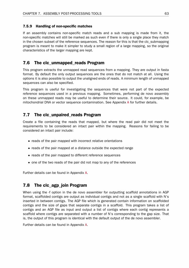
CHAPTER 7. ASSEMBLY POST-PROCESSING TOOLS 63
7.5.9 Handling of non-specific matches
If an assembly contains non-specific match reads and a sub mapping is made from it, thenon-specific matches will still be marked as such even if there is only a single place they matchin the chosen subset of the reference sequences. The reason for this is that the clc_submappingprogram is meant to make it simpler to study a small region of a large mapping, so the originalcharacteristics of the larger mapping are kept.
7.6 The clc_unmapped_reads ProgramThis program extracts the unmapped read sequences from a mapping. They are output in fastaformat. By default the only output sequences are the ones that do not match at all. Using theoptions it is also possible to output the unaligned ends of reads. A minimum length of unmappedsequences can also be specified.
This program is useful for investigating the sequences that were not part of the expectedreference sequences used in a previous mapping. Sometimes, performing de novo assemblyon these unmapped reads may be useful to determine their source. It could, for example, bemitochondrial DNA or vector sequence contamination. See Appendix A for further details.
7.7 The clc_unpaired_reads ProgramCreate a file containing the reads that mapped, but where the read pair did not meet therequirements to be considered an intact pair within the mapping. Reasons for failing to beconsidered an intact pair include:
• reads of the pair mapped with incorrect relative orientations
• reads of the pair mapped at a distance outside the expected range
• reads of the pair mapped to different reference sequences
• one of the two reads of the pair did not map to any of the references
Further details can be found in Appendix A.
7.8 The clc_agp_join ProgramWhen using the -f option in the de novo assembler for outputting scaffold annotations in AGPformat, scaffolded contigs are output as individual contigs and not as a single scaffold with N’sinserted in between contigs. The AGP file which is generated contain information on scaffoldedcontigs and the size of gaps that separate contigs in a scaffold. This program takes a list ofcontigs and an AGP file as input and output a list of contigs where each contig represents ascaffold where contigs are separated with a number of N’s corresponding to the gap size. Thatis, the output of this program is identical with the default output of the de novo assembler.
Further details can be found in Appendix A.

Chapter 8
Sequence preparation tools
8.1 The clc_adapter_trim ProgramTrims adapters from sequences.
Many sequencing technologies may leave whole or partial adapter or linker sequences in thereads for various reasons. The clc_adapter_trim program is used to find and remove suchadapters from the reads.
The clc_adapter_trim tool identifies likely adapters in reads and removes them. To account forsequencing errors known adapter sequence are aligned with each read. Matching positions inthese alignments score 1, while each mismatch costs 2 and each gap costs 3. By default, aregion that aligns with a score of at least 10 is considered a possible adapter region. The -coption can be used to change the default score threshold of 10.
By default, the clc_adapter_trim tool trims bases towards the 3´ end of reads using the followingapproach:
• For any read with only one region scoring equal to or higher than 10, that region isconsidered the be an adapter. The adapter region and all bases towards the 3´ end areremoved.
• For any read where there is no alignment to a known adapter sequence scoring 10 orgreater, the 3´ end of the read is checked for any possible sign of adapter. If found, suchbases will be removed. For example if a single nucleotide at the end of a read is identicalto the first nucleotide of the adaptor it will be removed since it may have come from anadaptor. The end match is defined as the longest match at the end of the read having anon-negative score when aligned to the adapter.
• For any read with more than one region aligning with a score equal to or higher than 10, theregion closest to the 3´ end is considered to be an adapter and removed along with anybases towards the 3´ end.
With the -e option it is possible to change the behavior so the reads are trimmed towards the 5´end of reads, rather than the 3´ end. In this case, the conditions described above are the same,with the directionality of the actions reversed.
The clc_adapter_trim program allows fine control over the behavior of the tool. For example,
64

CHAPTER 8. SEQUENCE PREPARATION TOOLS 65
• Should read sequences before or after the adapter be kept. The default action is to keepthe sequence before the adapter, but this can be altered using the -e option.
• Which reads should be kept. For example, reads where adapter was found are kept byusing the -t or -f options, and reads where the adapter was not found are kept by using the-u or -g options.
• Which adapter sequences should be searched for. One or several adapter sequences canbe used, using the -a and -d options, and for paired data, different adapters can be usedfor the first and second reads in the pairs by using the -j and -k options.
For adapter sequences given with the -a, -j or -k options, the reverse complement of the adaptersequences is automatically added to the list of adapters to search for.
Further details can be found in Appendix A.
8.2 Quality trimmingThe clc_quality_trim program is used to trim sequencing reads for low quality. The idea is to trimthe reads at one or both ends so that only a region of high-quality bases are left. This is doneby specifying a threshold value (using the ‘-c’ option) for low-quality base calls. The default valueis 20, which means that quality scores below 20 are marked as low quality. Since it is oftennot desirable to discard a high-quality region because of one isolated low-quality base, you canspecify the fraction of low-quality bases allowed in a region using the ‘-b’ option. The defaultvalue is 0.1 meaning that up to 10 % low-quality bases are allowed. The trim algorithm will then,for each read, find the longest region that fulfills these thresholds. Note that in some situationsthe full read will be discarded if no good quality regions can be found.
For paired data, two separate files are specified as output: one for the intact pairs (use the-p option for this output file) and one for the single reads whose mate was discarded duringtrimming (use the -o option for this output file).
There are other options to refine the quality trimming even more (see Appendix A).
8.2.1 Fastq quality scoring
The clc_quality_trim program requires an ASCII offset value for the quality scores in fastqformatted files. The default behavior is to automatically detect this offset from the input data, butin case that this fails it is also possible to set the offset manually. To set the offset correctly youneed to know the pipeline used to generate the original data and then set the offset accordinglyusing the -f option. Some examples of standard offset values for Illumina pipelines are:
• NCBI/Sanger & Illumina Pipeline 1.8 and later: 33
• Illumina Pipeline 1.2 and earlier: 64
• Illumina Pipeline 1.3 and 1.4: 64
• Illumina Pipeline 1.5 to 1.7: 64
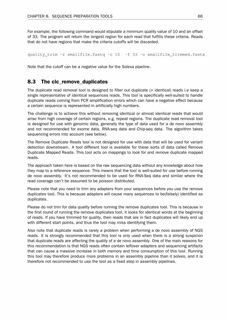
CHAPTER 8. SEQUENCE PREPARATION TOOLS 66
For example, the following command would stipulate a minimum quality value of 10 and an offsetof 33. The program will return the longest region for each read that fulfills these criteria. Readsthat do not have regions that make the criteria cutoffs will be discarded.
quality_trim -r smallfile.fastq -c 10 -f 33 -o smallfile_trimmed.fasta
Note that the cutoff can be a negative value for the Solexa pipeline.
8.3 The clc_remove_duplicatesThe duplicate read removal tool is designed to filter out duplicate (= identical) reads i.e keep asingle representative of identical sequences reads. This tool is specifically well-suited to handleduplicate reads coming from PCR amplification errors which can have a negative effect becausea certain sequence is represented in artificially high numbers.
The challenge is to achieve this without removing identical or almost identical reads that wouldarise from high coverage of certain regions, e.g. repeat regions. The duplicate read removal toolis designed for use with genomic data, generally the type of data used for a de novo assemblyand not recommended for exome data, RNA-seq data and Chip-seq data. The algorithm takessequencing errors into account (see below).
The Remove Duplicate Reads tool is not designed for use with data that will be used for variantdetection downstream. A tool different tool is available for these sorts of data called RemoveDuplicate Mapped Reads. This tool acts on mappings to look for and remove duplicate mappedreads.
The approach taken here is based on the raw sequencing data without any knowledge about howthey map to a reference sequence. This means that the tool is well-suited for use before runningde novo assembly. It’s not recommended to be used for RNA-Seq data and similar where theread coverage can’t be assumed to be poisson distributed.
Please note that you need to trim any adapters from your sequences before you use the removeduplicates tool. This is because adapters will cause many sequences to be(falsely) identified asduplicates.
Please do not trim for data quality before running the remove duplicates tool. This is because inthe first round of running the remove duplicates tool, it looks for identical words at the beginningof reads. If you have trimmed for quality, then reads that are in fact duplicates will likely end upwith different start points, and thus the tool may miss identifying them.
Also note that duplicate reads is rarely a problem when performing a de novo assembly of NGSreads. It is strongly recommended that this tool is only used when there is a strong suspicionthat duplicate reads are affecting the quality of a de novo assembly. One of the main reasons forthis recommendation is that NGS reads often contain leftover adapters and sequencing artifactsthat can cause a massive increase in both memory and time consumption of this tool. Runningthis tool may therefore produce more problems in an assembly pipeline than it solves, and it istherefore not recommended to use the tool as a fixed step in assembly pipelines.
CHAPTER 8. SEQUENCE PREPARATION TOOLS 67
8.3.1 Looking for neighbors
An example of a read duplication can be easily distinguished when mapping reads to a referencesequence as shown in figure 8.1.
Figure 8.1: Mapped reads with a set of duplicate reads, the colors denote the strand (green isforward and red is reverse).
The typical signature is a lot of reads starting at the same position, resulting in a sudden rise incoverage, and all reads have the same orientation (denoted by the color). In a normal data set,you will also see fluctuations in coverage as shown in figure 8.2, but they lack the two importantfeatures of duplicate reads: they do not all start at exactly the same position, and they are fromdifferent strands.
Figure 8.2: Rise in coverage.

CHAPTER 8. SEQUENCE PREPARATION TOOLS 68
The duplicate reads tool works directly on the sequencing reads, so there is no need to map thedata to a reference genome first (figures 8.2 and 8.2 show the reads mapped for illustrationpurposes). In short, the algorithm will look for "neighboring" reads (i.e. reads that share most ofthe read sequence but with a small offset) and use these to determine whether there is generallyhigh coverage for this sequence. If this is not the case, the read in question will be marked as aduplicate.
For certain sequencing platforms such as 454, the reads will have varying lengths - and this istaken into account by the algorithm as well.
SOLiD data is also supported, taking into account the dual base coding features of SOLiD data(color space).
8.3.2 Sequencing errors in duplicates
It is important to take sequencing errors into account when filtering duplicate reads. Imagine anexample with 100 duplicates of a read of 100 bp. If there is a random 0.1 % probability of asequencing error, it means that 10 of these reads have an error. If the algorithm only removedthe 90 identical reads, there will be 10 reads left with sequencing errors. This is a big problemsince the correct sequence is only represented once.
To address this issue, the duplicate read removal program accounts for sequencing errors whenit identifies duplicate reads. Specifically, reads are considered duplicates if:
• they share a common sequence of at least 20 bases1 in the beginning, or at any of fourother regions distributed evenly across the read, and
• the rest of the read has an alignment score above 80 % of the optimal score, where theoptimal score is what a read would get if it aligned perfectly to the consensus for a groupof duplicates.
Please note that these thresholds for similarity are not enough for reads to be marked asduplicates - they just define how different reads are allowed to be and still be consideredduplicates. Rather, the duplicates are identified as explained in section 8.3.1.
8.3.3 Paired data
For paired reads, we check whether the sequences in different pairs mapping in a given regionhave their first 10 base pairs identical. If they do, they are marked as potential duplicate reads.(We have found this route works better than a statistical route in the case of paired data.) Wethen check our proposed list of duplicates to look for false positives. We also do a check forclosely related variants of those sequences we now believe to represent duplicate reads.
The algorithm also takes sequencing errors into account when filtering out paired data.
8.3.4 Known limitations
The duplicate read removal has a limitation when there are duplicate reads that contain severalalleles. The algorithm will identify if there are duplicate reads to be removed, but it is not
1For paired reads, this is only 10 bases.

CHAPTER 8. SEQUENCE PREPARATION TOOLS 69
able to distinguish between sequencing errors and true variation in the reads. So if you have aheterozygous SNP in such an area, you may risk that only one of the alleles are preserved.
8.3.5 Example of duplicate read removal
The following command outputs all reads to coli_reads_nodup.fa that are not identified asduplicates from the paired reads contained in coli_reads_1/2.fa and coli_reads_2/2.fa.
clc_remove_duplicates -p -r -i coli_reads_1/2.fa coli_reads_2/2.fa-o coli_reads_nodup.fa
The program runs only in a single thread and for large data set it would be convenient to runmultiple instances at the same time for each data file.
8.4 The clc_sample_reads ProgramThis tool extracts a subset of reads where the size of the subset is a percentage of the inputsize. Sampling is done in a pseudo-random way, which does not guarantee that the extractedsubset comprises an exact percentage of the input reads. The input reads can be provided inboth interleaved and non-interleaved format and reads marked as paired are kept together.
Read sampling can be useful for reducing coverage of datasets with a very high coverage (>500xcoverage) in preparation for a de novo assembly. A reduction in coverage makes the assemblyrun faster and reduces the chance of having overlapping errors in the reads, thus increasing theassembly quality.
See Appendix A for full usage information.
8.5 The clc_sort_pairs ProgramThe clc_sort_pairs program takes two SOLiD read files, or two Ion Torrent read files, as input andgenerates as output a file containing paired reads and a file containing unpaired reads. Here theread names are used to sort the reads. This tool is necessary because pairing of the reads inthese cases is based on the read names rather than just the position within the file, as wouldbe the case for Illumina data. That is, paired reads for these data types need to be sorted, andpaired reads separated from single reads.
To properly handle the input sequence data, the read names within the files must match certainpatterns. These are:
Ion Torrent: [anytextinfo]:[number]:[number]
Solid: [number]_[number]_[number]_[R3/F3/F5/F5-P2/F5-BC]
In the case of Solid data, reads in one file of the pair should end in one of the patterns above,and reads in the other file of the pair should end with one of the other patterns. For example,one file might contain reads with names ending in R3, while reads in the other file have names

CHAPTER 8. SEQUENCE PREPARATION TOOLS 70
ending in F5, or reads in one file might contain names ending in F3, while reads in the other filehave names ending in F5, and so on.
Reads within a given file must be named consistently. That is, if a read has a name ending witha particular pattern, for example F5, then all reads in that file must have names ending in F5.
Please note that in the case of Solid data, the following combinations for the read names in apair of files are not allowed:
F3 + F3R5 + F5R3 + R3R3 + F5F5 + R3
As mentioned in the Input Data section earlier in the manual, the full sequence of any readcontaining one or more . symbols, present in a .csfasta format file, will be converted to containonly N characters.
Further details are provided in Appendix A.
8.6 The clc_split_reads Program (for 454 paired data)The 454 sequencing technology can produce paired read files where the two paired readfragments are contained within the same read, separated by a linker sequence. The linker maybe placed anywhere in the read or even outside the read, so not all the reads will necessarilycontain a pair. The clc_split_reads program finds the linker sequence and creates two new files,one with paired reads and one with unpaired reads.
Like adapter regions, linker regions may contain sequencing errors. With this in mind, theclc_split_reads tool identifies likely linker sequences by initially carrying out an alignmentbetween the known linker sequence and each read. The alignment is global in terms of the linkerand local in terms of the reads. That is, the whole linker must align to part of the read. Matchingpositions in these alignments score 1, while each mismatch costs 2 and each gap costs 3. Foralignments found at the ends of reads, any non-matching linker bases that extend beyond theend of the read are not penalized.
By default, a region that aligns with a score of at least 10, or the length of the linker if less than10, is considered a good enough match to identify a linker region.
If a match to the linker sequence with a score between 0 and 9 is found, the read will still besplit, but in this situation the following will happen:
• The two parts of the read that have just been split are put into the singles list (not the pairedlist). The reasoning behind this is that since the linker did not match with a good enoughscore, the match location identified might not have been correct. If this was the case,marking such split sequences as a pair would mean that the paired distance informationwould be used in a de novo assembly, and this could end up being misleading within theassembly process.
• Any linker matches identified at the end of the read will also be trimmed. This extra trimming
CHAPTER 8. SEQUENCE PREPARATION TOOLS 71
stage is carried out due to the possibility that the internal linker match identified might nothave been correct.
The following situations are particularly detrimental to de novo assembly, and the clc_split_readsprogram tries to ensure they are avoided:
• Reads contain some remaining section of the linker sequence
• Reads are categorized as a pair when they should not be
In some cases, the start or end of a read is in the middle of the linker. In such cases, the linkersequence is still removed, and the read is put into the file with unpaired reads. If only very fewnucleotides of the linker overlap with the read, they are also removed, even though they may notcome from the linker. In the case where only a single nucleotide at the start and/or end of theread may come from a linker, it is removed. The rationale is that it is better to discard a fewnucleotides and be sure there is no adapter sequence left, since remaining linker sequence isproblematic for de novo assembly.
The ‘-m’ option can be used to specify the minimum read length. Only reads this long or longerwill be reported. The default value is 15. This becomes important when the linker is close tothe start or end of the read, and only a small fragment is left on one side of the linker. If thatsmall fragment is below the specified minimum length, it is discarded along with the linker. Theremaining part of the read will be written to the unpaired file.
Further details of the options for this tool are provided in Appendix A.
8.7 The clc_overlap_reads ProgramIn cases where paired end library preparation methods use a relatively short fragment size, someread pairs will overlap. These overlapping reads can be handled as standard paired-end data.
However, in some situations it can be useful to merge the overlapping pairs into a single read.The benefit is that you get longer reads, and that the quality improves (normally the quality dropstowards the end of a read, and by overlapping the ends of two reads, the consensus read nowreflects two read ends instead of just one).
This joining of overlapping reads can be done using the clc_overlap_reads program. It aligns theends of each read within pairs to see if there is evidence that they overlap. If the alignment ofthese read ends is relatively good, the reads are joined into one read and put in an output file forsingle (joint) reads. If there is no evidence of the reads overlapping, the original pair of reads isput in an output file for paired reads.
The nucleotides in the overlapping region of a joint read are assigned a quality score of 40 (veryhigh quality) if the two reads agree on the nucleotide. Otherwise the nucleotide with the highestquality is chosen and its quality score is retained.
By default, the alignment between the ends of two reads must have a minimum length of 10positions and a minimum similarity of 90% for the reads to be considered overlapping. Theseparameters can be adjusted using the various options for the program. The default is that thefirst read of each pair is a forward read and the other one is a backward read. This can also beadjusted.

CHAPTER 8. SEQUENCE PREPARATION TOOLS 72
In cases where reads contain an adapter sequence at the read ends, the adapter sequenceneeds to be removed (see figure 8.3). The option --autoadapter enables free gaps at the readends and leaves out unaligned read ends, i.e. any adapter sequences will not be included in theresult.
Further details of the overlap reads options are provided in Appendix A.
Figure 8.3: Illustration of two reads originating from a fragment which is shorter than the readlength. Both reads contain adapter sequences in the read ends which needs to be removed whenoverlapping the reads.
Chapter 9
Format conversion tools
9.1 The clc_cas_to_sam ProgramThis tool converts a cas format file to sam or bam format format file.
The clc_cas_to_sam program takes a cas file as input and produces a corresponding SAM fileor BAM file. The format generated depends on the filename you choose. If you choose an outputfile name with the suffix .sam, the output format will be SAM. If you choose an output file namewith the suffix .bam, the output format will be BAM.
Please note that the read file(s) that you used in generating the cas file must be present in thesame relative location to the cas file as they were when you ran the mapping. This is because,unlike cas format files, SAM and BAM files include all the read data. Thus the read data needsto be present in order to make a valid SAM or BAM file. This also means that the SAM or BAMfiles created will generally be substantially larger than the cas file they were generated from.
When writing a sam/bam file, each read is given a read mapping quality (MAPQ) score of either0 or 60. The value 60 is given to reads that mapped uniquely. The value 0 is given to reads thatcould map equally well to other locations besides the one being reported in the BAM file.
The SAM or BAM file created using the clc_cas_to_sam tool is not sorted or indexed. Thesesteps can be necessary for some types of downstream processing and can be done using thesamtools sort program (see http://samtools.sourceforge.net/).
Like cas format files, SAM and BAM files do not contain the reference sequence data.
Further details of the command line options for this tool are provided in Appendix A.
Further details about the SAM and BAM formats can be found at http://samtools.sourceforge.net/.
9.2 The clc_sam_to_cas ProgramThis tool converts a read mapping in sam or bam format to a cas format file.
The clc_sam_to_cas tool converts SAM or BAM files to cas format. Like cas format files, SAMand BAM files do not contain the reference sequence data, so the reference sequences needto be provided when running this command. This is so that the required information can be
73
CHAPTER 9. FORMAT CONVERSION TOOLS 74
generated for the cas file.
You also need to provide a destination for the sequencing read data to be written to when runningthis program.
Further details of the command line options for this tool are provided in Appendix A.
9.3 The clc_convert_sequences ProgramThe primary purpose of this tool is to convert sequences to fasta or fastq format. However, it cancurrently be used for a variety of sequence conversion related functions. These include:
• Convert from one format to a fasta format file or to a fastq format file.
• Merge separate forward and reverse read files into a single, interleaved paired data file.
• Remove sequence names from within a file (to save space).
• Create a fastq format file from (separate) sequence and quality files.
Input formats supported for some or all functionality:
• fasta
• fastq
• genbank
• sff
• csfasta
Export formats are fasta or fastq.
See Appendix A for full usage information.

Appendix A
Options for All Programs
Please find the list of options for all programs in the online version of the user manual at http://resources.qiagenbioinformatics.com/manuals/clcassemblycell/current/index.php?manual=Options_All_Programs.html
75
Appendix B
Third Party Libraries
The CLC Assembly Cell for windows includes a number of third party libraries.
Please consult the files named NOTICE and LICENSE in the assembly cell installation directoryfor the legal notices and acknowledgements of use.
For the code found in this product that is subject to the Lesser General Public License (LGPL)you can receive a copy of the corresponding source code by sending a request to our supportfunction.
76
Bibliography
[Gnerre et al., 2011] Gnerre, S., Maccallum, I., Przybylski, D., Ribeiro, F. J., Burton, J. N.,Walker, B. J., Sharpe, T., Hall, G., Shea, T. P., Sykes, S., Berlin, A. M., Aird, D., Costello,M., Daza, R., Williams, L., Nicol, R., Gnirke, A., Nusbaum, C., Lander, E. S., and Jaffe,D. B. (2011). High-quality draft assemblies of mammalian genomes from massively parallelsequence data. Proceedings of the National Academy of Sciences of the United States ofAmerica, 108(4):1513--8.
[Li et al., 2010] Li, R., Zhu, H., Ruan, J., Qian, W., Fang, X., Shi, Z., Li, Y., Li, S., Shan, G.,Kristiansen, K., Li, S., Yang, H., Wang, J., and Wang, J. (2010). De novo assembly of humangenomes with massively parallel short read sequencing. Genome research, 20(2):265--72.
[Zerbino and Birney, 2008] Zerbino, D. R. and Birney, E. (2008). Velvet: algorithms for de novoshort read assembly using de Bruijn graphs. Genome Res, 18(5):821--829.
[Zerbino et al., 2009] Zerbino, D. R., McEwen, G. K., Margulies, E. H., and Birney, E. (2009).Pebble and rock band: heuristic resolution of repeats and scaffolding in the velvet short-readde novo assembler. PloS one, 4(12):e8407.
77
Index
Bibliography, 77
Cores, maximum limit, 12CPU architectures, 12CPU cores, maximum limit, 12
References, 77
System requirements, 12
78